Replenishment and connectivity of reef fish populations in ...
213
This file is part of the following reference: Abesamis, Rene A. (2011) Replenishment and connectivity of reef fish populations in the central Philippines. PhD thesis, James Cook University. Access to this file is available from: http://eprints.jcu.edu.au/27947/ The author has certified to JCU that they have made a reasonable effort to gain permission and acknowledge the owner of any third party copyright material included in this document. If you believe that this is not the case, please contact [email protected] and quote http://eprints.jcu.edu.au/27947/ ResearchOnline@JCU
Transcript of Replenishment and connectivity of reef fish populations in ...

This file is part of the following reference:
Abesamis, Rene A. (2011) Replenishment and
connectivity of reef fish populations in the central
Philippines. PhD thesis, James Cook University.
Access to this file is available from:
http://eprints.jcu.edu.au/27947/
The author has certified to JCU that they have made a reasonable effort to gain
permission and acknowledge the owner of any third party copyright material
included in this document. If you believe that this is not the case, please contact
[email protected] and quote http://eprints.jcu.edu.au/27947/
ResearchOnline@JCU

Replenishment and connectivity of reef fish populations
in the central Philippines
Thesis submitted by
Rene A. Abesamis MSc
in July 2011
for the degree of Doctor of Philosophy
at the School of Marine and Tropical Biology
James Cook University

ii
Statement on the Contribution of Others
This thesis was funded by an Australian Research Council (ARC) Grant to Prof.
Garry R. Russ, through the ARC Centre of Excellence for Coral Reef Studies.
Additional support during fieldwork in the Philippines was given by Prof. Angel C.
Alcala through the Silliman University-Angelo King Centre for Research and
Environmental Management (SUAKCREM). I received an Endeavour International
Postgraduate Research Scholarship and a James Cook University Postgraduate Research
Scholarship at the School of Marine and Tropical Biology from June 2007 to December
2010.
I performed the research for Chapter 2 in collaboration with SUAKCREM in
Dumaguete City, Negros Oriental, Philippines. The monthly spawning surveys were
conducted with the assistance of Claro Renato Jadloc. Mr. Jadloc was instrumental in
obtaining monthly fish samples, development of gonad staging scales, identification of
the different oocyte stages and estimation of batch fecundities of the four species that
were studied. Mr. Jadloc will be a co-author of the paper to be submitted for publication
based on Chapter 2. He will also be a co-author of a paper (separate from this thesis) on
the reproductive biology of the four species that were studied, which formed part of his
MSc thesis at Silliman University.
I performed the research for Chapter 4 in collaboration with SUAKCREM and
the University of the Philippines-Marine Science Institute (UPMSI). Brian Stockwell of
SUAKCREM collected the data on reef fish species distributions across the Bohol Sea
and gave his consent for the use of this data for Chapter 4. The data on benthic habitat
were collected by myself and several SUAKCREM staff: Brian Stockwell, Claro Renato
Jadloc, Jasper Maypa, and Marco Innocencio. The code for the Lagrangian (particle
tracking) larval dispersal model was originally written in C by Prof. Cesar L. Villanoy
of UPMSI. Initial testing of the model for the Bohol Sea was done by Erlinda Salamante
and Charina Repollo of UPMSI. The final model used in the simulations was developed
from early model configurations by Lawrence Bernardo of UPMSI in consultation with
Prof. Villanoy and myself. Mr. Bernardo made improvements to the advection-diffusion
and interpolation schemes, streamlined the code so it could be efficiently run on cluster
computing systems, generated the needed input data, and adapted the model to meet the
objectives of this research. The application of the model to address questions about the
iii
physical oceanography of the Bohol Sea is part of Mr. Bernardo’s MSc thesis at
UPMSI. Mr. Stockwell, Prof. Villanoy and Mr. Bernardo will be co-authors of the paper
to be submitted for publication based on Chapter 4.
The larval dispersal model developed for the Bohol Sea in collaboration with
Mr. Bernardo and Prof. Villanoy of UPMSI was modified to address the research
questions in Chapter 5. Mr. Bernardo and Prof. Villanoy will be co-authors of the paper
to be submitted for publication based on this Chapter.
I am extremely grateful to the Philippine Department of Science and
Technology-Advanced Science and Technology Institute (DOST-ASTI) at the
University of the Philippines-Diliman for granting access to its state-of-the-art high
performance computing facility to run the larval dispersal models for Chapters 4 and 5.
Daily wind and rainfall data were generously provided by the DOST- Philippine
Atmospheric, Geophysical and Astronomical Services Administration (PAGASA)
weather station at Dumaguete Airport. Additional infrastructure was provided by
SUAKCREM and the Silliman University-Institute of Environmental and Marine
Science.
All research procedures reported in the thesis received approval from the Animal
Ethics Committee at James Cook University.
iv
Acknowledgements
This thesis would not have been possible without Garry Russ. No words can
really express how grateful I am to Garry for being an excellent supervisor, mentor and
friend. I am also very thankful to Angel Alcala for his unwavering support of this
research. Dr. Alcala always made time to sit down with me if I needed a sounding board
for my ideas, even if he had an impossible schedule to keep (as always). I consider
myself extremely lucky for having been given the opportunity to work with Garry and
Dr. Alcala and pursue some of the most important and interesting questions about
marine reserves.
I am very grateful to the Australian Commonwealth Government for the
International Postgraduate Research Scholarship (IPRS) that I received from June 2007
to December 2010. I also thank the School of Marine and Tropical Biology for
supplementing the IPRS with a JCU Postgraduate Research Scholarship. Research for
this thesis was supported by a grant to Garry Russ from the Australian Research Council
CoE for Coral Reef Studies. I also received support in various forms from the following
institutions: Silliman University-Angelo King Centre for Research and Environmental
Management (SUAKCREM), SU-Institute of Environmental and Marine Science (SU-
IEMS), University of the Philippines-Marine Science Institute (UP-MSI) and two
agencies of the Philippine Department of Science and Technology – the Advanced
Science and Technology Institute (DOST-ASTI) and the Philippine Atmospheric,
Geophysical and Astronomical Services Administration (DOST-PAGASA).
This thesis would also not have been successful without the talents and
generosity of four key persons: Brian Stockwell, Renclar Jadloc, Prof. Cesar ‘K’
Villanoy and Lawrence Bernardo. Brian kindly shared his data on reef fish species
distributions in the Bohol Sea. Renclar was instrumental in the success of monthly
spawning and recruitment surveys. Without K and Lawrence, modelling of larval
dispersal in the Bohol Sea would have been impossible. I look forward to working with
all of them again in the near future.
Many other individuals and institutions also contributed to the completion of this
thesis in one way or another, including: Geoff Jones, Mike Kingsford, Howard Choat,
Jonathan Kool, Hilconida Calumpong, Analie and Francia Candido, Liberty Pascobello,
Mario Pascobello, Dioscoro Innocencio, Job Tagle, Toni Yucor, Edsin Culi and his staff

v
at PAGASA, Erlinda Salamante, Charina Repollo, Perry Aliño, Mags Quibilan, Rollan
Geronimo, Nick Graham, Phil Munday, Maya Srinivasan, D.C. Lou, Olive Cabrera,
Zacharias Generoso, Jasper Maypa, Abner Bucol, the late Yayoy Uy and his excellent
staff and boat crew at KDU Dive Shop, the Local Government Unit (LGU) of Dauin
and Oslob, Bantay Dagat of Sumilon Is., Bantayan (Dumaguete), Apo Is., Dauin
Poblacion 1 and Masaplod Norte marine reserves, Vanessa Messmer, Hugo Harrison,
Alex Anderson, Tom Holmes, Rebecca Weeks, Richard Evans, Philippa Mantel, and the
Russ family.
The Abesamis and Palomar families were always ready to help when I or my
growing family moved around from place to place (Dumaguete, Manila, Townsville) as
I worked on this thesis.
Lastly, to Nadia, Mayumi, and Amaya thank you for your warmth, patience and
love.
vi
Abstract
The dynamics of reef fish populations at lower latitudes are not well understood,
particularly in the Coral Triangle (composed of the Philippines, Malaysia, Indonesia,
Timor Leste, Papua New Guinea and the Solomon Islands), where the monsoons
(shifting tradewinds) are potential drivers of seasonality of reproduction and
recruitment. Such dynamics will also be influenced by the degree to which local
populations self-replenish or rely on larval replenishment from other populations.
However, few have investigated the effects of the monsoons on the replenishment of
reef fish populations. Furthermore, the extent of ecologically-significant larval dispersal
of reef fishes, in general, remains unclear. Understanding the patterns and key processes
behind population replenishment and larval dispersal are critical to the application of
no-take marine reserve networks as conservation and fisheries management tools. This
thesis addresses knowledge gaps about the patterns of reproduction, recruitment and
larval connectivity of reef fish populations in the central Philippines, the epicentre of
reef fish biodiversity in the Coral Triangle.
The questions that this thesis addresses are especially relevant to the use of no-
take marine reserves for reef conservation and fisheries management in the Philippines,
a developing archipelagic nation with a vast coral reef area, a large and rapidly growing
human population and a great number of small, community-based marine reserves.
Most coastal communities in the Philippines are poor and have few employment
alternatives. Many communities rely on coral reefs for food and livelihood. No-take
marine reserves in the Philippines are regarded as a viable option to conserve and
manage coral reefs that is acceptable to local stakeholders.
This thesis consists of four related studies. In the first study, I tested the
prevailing notion that spawning peaks of reef fish at lower latitudes are timed to take
advantage of weaker winds during inter-monsoonal periods, supposedly to limit
advection and enhance survivorship of larvae. The monthly spawning patterns of four
species of reef fish (2 fusiliers, 1 surgeonfish and 1 damselfish) were studied for 11-22
months. All four species showed protracted spawning periods. However, results
suggested that the monsoons affect reproduction in ways that are not consistent with the
above hypothesis. Conditions advantageous to larval survival may not be restricted to
the inter-monsoonal periods. An alternative explanation is that the spawning patterns

vii
probably reflected temperature, rainfall, wind or wave action more directly influencing
the spawning of adults, as opposed to adaptation of the timing of reproduction to ensure
higher survivorship of larvae in the pelagic environment. The complex effects of the
monsoons on reproduction in reef fishes warrant further study.
In the second study, I investigated the patterns of recruitment (larval settlement)
of 120 species of reef fish almost every month for 20 consecutive months at two island
and two coastal locations. Recruitment was found to occur throughout the year. Most
species exhibited protracted recruitment seasons (up to 9-11 months). However, a
predictable annual peak in community-wide recruitment of reef fishes was detected,
coinciding with the weakening of monsoon winds and higher sea surface temperature.
The annual pattern of recruitment was fairly consistent across 11 sites and between the
two years sampled. The same recruitment pattern was also found in the two families that
dominated monthly recruitment to reefs, the damselfishes and the wrasses,
notwithstanding a 10-fold difference in overall abundance of recruits of these two
families. These findings implied a far-reaching influence of the monsoons on
recruitment of reef fishes at lower latitudes.
In the third study, I determined the extent of potential larval connectivity among
reef fish populations across a 300-km-wide region of the Bohol Sea in the central
Philippine archipelago, by combining two very different methods: 1) analysis of species
assemblage patterns (presence/absence of 216 species at 61 sampling sites) and
associated habitat patterns; and 2) modelling of reef fish larval dispersal patterns. The
results of the two methods independently suggested probable connectivity within a large
group of sites situated in an internal sea where a dominant westward current is present.
The presence of potentially significant connectivity among these sites, and their lack of
strong connectivity with other sites were probably strongly influenced by the local
oceanographic setting and habitat. The results were consistent with present knowledge
of the spatial scales of ecologically-relevant larval dispersal in reef fishes (10’s of
kilometres). The study provided a framework for connectivity within existing networks
of no-take marine reserves in the region.
In the final study, I estimated the probable extent of recruitment subsidy (net
larval export) and larval connectivity of 39 small (< 1 km2) no-take marine reserves
within a more limited (135 x 70 km) region of the Bohol Sea in the central Philippines.
The reserves were estimated to occupy about 6% of total reef area in that region. I used
a simple exponential model of population recovery to estimate the increase in larval

viii
production of large predatory reef fishes inside reserves over time. Larval dispersal and
recruitment were simulated using a larval dispersal model. The model simulations
showed that a 3.5-fold (~250%) increase in recruitment to fished areas may result from
a 55-fold increase in larval production inside reserves if all reserves were effectively
protected for 20 years. Lesser larval subsidies are likely to more than replace losses in
yield due to reserve creation but they will be difficult to detect because of temporal and
spatial variation in recruitment. The strength of larval connectivity between reserves
increased dramatically (up to ~20-fold) with greater larval production. These findings
highlight the importance of protecting reserves over the long-term (decades) and
establishing reserve networks that interact effectively via larval exchange in order for
reserves to sustain reef fisheries in highly overfished areas and the reserve networks of
which they are a part.
A synthesis of the results of this thesis highlighted the importance of the
monsoons and local geographic setting in shaping the patterns of replenishment and
connectivity of reef fish populations in the Coral Triangle. The implications of potential
relationships between the monsoons and the dynamics of reef fish populations amidst a
changing climate were also explored. Finally, future research that can validate
ecologically-relevant larval connectivity within reserve networks and encourage the
long-term protection of reserves were proposed.

ix
Table of Contents
Statement on the Contribution of Others…………………………………………... ii
Acknowledgements………………………………………………………………… iv
Abstract……………………………………………………………………………. vi
Table of Contents…………………………………………………………………... ix
List of Tables……………………………………………………………………..... xiii
List of Figures……………………………………………………………………… xv
List of Appendices…………………………………………………………………..xviii
Chapter 1. General Introduction……………………………………………... 1
Chapter 2. Seasonality of spawning of reef fishes in a monsoonal environment
Abstract……………………………………………………………. 10
2.1 Introduction…………………………………………………… 11
2.2 Materials and methods……………………………………….. 13
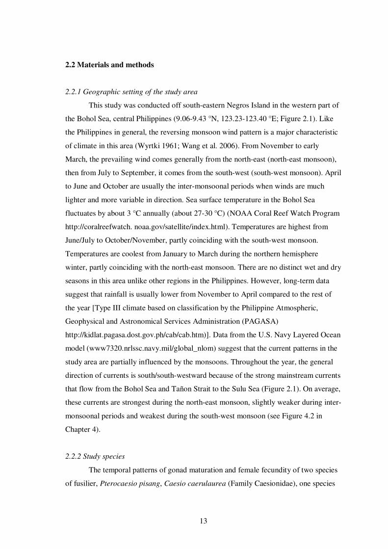
2.2.1 Geographic setting of the study area..……..………… 13
2.2.2 Study species…………………………………………. 13
2.2.3 Monthly sampling……………………………………..16
2.2.4 Macroscopic examination of gonads………………… 17
2.2.5 Histological examination of ovaries…………………..17
2.2.6 Examination of temporal patterns of spawning……… 19
2.2.7 Estimation of batch fecundity…………………………20
2.3 Results…………………………………………………………. 21
2.3.1 Sample size, size range and sex ratio…………………21
2.3.2 Accuracy of macroscopic staging of ovaries………… 21
2.3.3 Temporal patterns of spawning……………………….23
2.3.4 Estimates of batch fecundity…………………………..29
2.4 Discussion……………………………………………………... 29
Chapter 3. Patterns of recruitment of reef fishes in a monsoonal environment

x
Abstract……………………………………………………………. 37
3.1 Introduction…………………………………………………… 38
3.2 Materials and methods……………………………………….. 39
3.2.1 Geographic setting of the study area…..…………….. 39
3.2.2 Study sites……………………………………………..41
3.2.3 Visual census of recruits……………………………... 41
3.2.4 Weather data and sea surface conditions……………. 44
3.2.5 Data analyses ………………………………………... 45
3.3 Results…………………………………………………………. 46
3.4 Discussion……………………………………………………....54
Chapter 4. Predicting connectivity in a marine reserve network from reef fish
assemblage patterns and larval dispersal models
Abstract……………………………………………………………. 59
4.1 Introduction…………………………………………………… 60
4.2 Materials and methods……………………………………….. 64
4.2.1 The study region…..………………………………….. 64
4.2.2 Reef fish and benthic habitat data…………………….67
4.2.3 Analyses of reef fish and environmental data………... 69
4.2.4 Individual-based biophysical model…………………. 70
4.2.5 Simulations of larval dispersal………………………..72
4.2.6 Analyses of larval dispersal data…………………….. 73
4.3 Results…………………………………………………………. 75
4.3.A General patterns…………………………………… 75
4.3.A.1 Fish species assemblage patterns………….. 75
4.3.A.2 Fish species assemblage patterns vs.
environmental variables……………………. 78
4.3.A.3 Patterns of larval dispersal
predicted by biophysical models…………… 80

xi
4.3.A.4 Fish species assemblage patterns vs.
predicted levels of connectivity…………….. 84
4.3.B Pair-wise comparisons of groups of sites
generated by hierarchical clustering
of species assemblage patterns…………………….. 84
4.3.B.1 Group A vs. Group H………………………. 86
4.3.B.2 Group B vs. Group H……………………… 86
4.3.B.3 Group C vs. Group H……………………… 89
4.3.B.4 Group E vs. Group H………………………. 90
4.3.B.5 Group F vs. Group H……………………… 90
4.3.B.6 Group G vs. Group H……………………… 91
4.3.B.7 Group I vs. Group J………………………... 91
4.4 Discussion……………………………………………………... 92
Chapter 5. Potential recruitment subsidy and connectivity of small no-take
marine reserves in the central Philippines
Abstract…………………………………………………………….101
5.1 Introduction…………………………………………………… 102
5.2 Materials and methods……………………………………….. 104
5.2.1 Background and physical setting of the study area….. 104
5.2.2 No-take marine reserves……………………………....106
5.2.3 Larval dispersal model………………………………..107
5.2.4 Larval production from and recruitment to
reserves and fished areas……………………………... 107
5.2.5 Model simulations……………………………………. 111
5.2.6 Data analysis………………………………………… 113
5.3 Results…………………………………………………………. 114
5.4 Discussion……………………………………………………... 120

xii
Chapter 6. General Discussion………………………………………………... 125
6.1. Synthesis – the importance of the monsoons and local
geographic setting to replenishment and connectivity
of reef fish populations…………………………………………… 125
6.2 Climate change and the influence of the monsoons
on reef fish population dynamics………………………………… 129
6.3 Reserve network goals and the future of
ad hoc reserve networks in the Philippines..……………………..130
Bibliography………………………………………………..................................... 133
Appendices………………………………………………………………………... 168

xiii
List of Tables
Chapter 2
Table 2.1 Known maximum size of Pterocaesio pisang, Caesio caerulaurea,
Naso minor and Pomacentrus moluccensis and the size ranges of male
and female individuals of each species in monthly samples……………….. 15
Table 2.2 Maturity stages of gonads of Pterocaesio pisang, Caesio caerulaurea,
Naso minor and Pomacentrus moluccensis………………………………...18
Table 2.3 Results of microscopic examination of ovaries to assess the accuracy
of estimating maturity stage based on external appearance………………... 22
Table 2.4 Spearman rank correlations (rs) of monthly proportions of individuals
with active gonads (represented by ♂ for testes and ♀ for ovaries) and
monthly female gonadosomatic indices (represented by ♀GSI) versus
monthly average sea surface temperature (SST), total rainfall or average
wind speed.………………….........................................................................25
Table 2.5 Results of 2-way ANOVA testing for significant differences in the
density of hydrated (or largest) oocytes among regions of the lobe
(i.e., anterior, median and posterior) and between the lobes of
ovaries of Pterocaesio pisang, Caesio caerulaurea, Naso minor
and Pomacentrus moluccensis……………………………………………... 31
Table 2.6 Estimates of batch fecundity for Pterocaesio pisang, Caesio
caerulaurea, Naso minor and Pomacentrus moluccensis………………….. 31
Chapter 3
Table 3.1 Summary of 1-way ANOVAs and subsequent planned contrasts to
xiv
determine significant differences in average recruit densities and species
richness among 19 months, between two years (2008 vs. 2009) and
between seasons……………………………………………………………. 49
Table 3.2 Summary of regression models to assess the potential effects of
environmental variables on temporal patterns of recruitment……………... 50
Chapter 4
Table 4.1 Combinations of predicted larval exchange between, and measured
habitat and species assemblage structure within, two theoretical sites……. 63
Table 4.2 Predicted levels of connectivity between 6 groups (A, B, C, E, F and G)
and the major Bohol Sea group (H) (1. to 6.) and between two subgroups
(I vs. J) of the main Bohol Sea group (7.)………………………………….. 85
Table 4.3 Summary of results of SIMPER analysis……………………………….. 88
Table 4.4 Summary of information required to infer the presence and probable
extent of larval connectivity between sampling sites……………………….93
Chapter 5
Table 5.1 List of the 39 reserves situated on reefs within the study area…………..108
Table 5.2 Estimated total adult biomass, spawning female biomass, number of
female spawners (M) and egg output (E) and effective larval output for
one unit (i.e., 40,000 m2) of fished area, a newly-established reserve
and for reserves with different durations of protection (DOP)…………….. 112

xv
List of Figures
Chapter 1
Figure 1.1 Map of the Coral Triangle region……………………………………… 3
Figure 1.2 Results of a literature survey to determine the number of publications
on the topic of a) reef fish population dynamics and b) marine reserves
or marine protected areas in the Coral Triangle versus the Great Barrier
Reef (GBR) and the Caribbean…………………………………………….. 5
Chapter 2
Figure 2.1 Map of the study area showing the sites where fish samples were
obtained for the spawning surveys…………………………………………. 14
Figure 2.2 Monthly gonad maturation patterns of Pterocaesio pisang versus
environmental variables……………………………………………………. 24
Figure 2.3 Monthly gonad maturation patterns of Caesio caerulaurea versus
environmental variables……………………………………………………. 27
Figure 2.4 Monthly gonad maturation patterns of Naso minor versus
environmental variables…………………………………………………… 28
Figure 2.5 Monthly gonad maturation patterns of Pomacentrus moluccensis versus
environmental variables……………………………………………………. 30
Chapter 3
Figure 3.1 Map of the study area showing the two islands (Sumilon and Apo)
and two coastal locations (Dumaguete and Dauin) where recruitment
of reef fishes were monitored over a 20-month period…………………….. 40

xvi
Figure 3.2 Temporal patterns of sea surface temperature, wind speed and
rainfall versus temporal patterns of recruit density and species richness
averaged for all sites…………………………………………………………47
Figure 3.3 Temporal patterns of total recruit density and species richness
averaged across all sites……………………………………………………. 51
Figure 3.4 Durations of the recruitment period (months) of the 37 most
abundant species (grouped into 7 families in this figure) estimated
using two thresholds of recruit abundance per month: ≥ 1% and ≥ 5%
of adjusted total abundance in one year……………………………………. 52
Figure 3.5 Summary of the timing of recruitment peaks of the 37 most
abundant species…………………………………………………………… 53
Chapter 4
Figure 4.1 Maps of the study region (Bohol Sea and adjacent bodies of water)….. 65
Figure 4.2 Annual trend in current patterns within the study region
represented by three months: January, May and August…………………... 66
Figure 4.3 Dendrogram showing hierarchical clustering of 61 sites based
on the Bray-Curtis similarity measure using data on reef fish
species composition (presence/absence)…………………………………… 76
Figure 4.4 Left side of the figure shows Non-metric Multi-Dimensional Scaling
(MDS) plots of species assemblages at each of 61 sites based on
Bray-Curtis similarity measure. Right side of the figure shows the
geographic locations of groups of sites formed at each level
of similarity………………………………………………………………… 77
Figure 4.5 Principal Components Analysis (PCA) plot of normalised
xvii
environmental data from 61 sampling sites…………………………………79
Figure 4.6 Dispersal probability matrices resulting from simulations of larval
dispersal using PLD values of 15, 30 and 45 days………………………… 81
Figure 4.7 Distances of larval dispersal (mean, modal range and maximal
range) from each node according to simulations using the
biophysical model………………………………………………………….. 82
Figure 4.8 Nodes ranked according to index of overall connectivity resulting
from simulations using PLD values of 15, 30 and 45 days…………………83
Figure 4.9 Habitat preferences of the species of reef fish that contributed
most to the dissimilarity between groups of sites formed by
hierarchical clustering…………………………………………………….. 87
Chapter 5
Figure 5.1 Map of the study area showing the 39 no-take marine reserves……….. 105
Figure 5.2 Average recruitment to fished areas within the entire study area
for five cases of larval production from reserves and fished areas………… 115
Figure 5.3 Spatial distribution of recruitment subsidy from reserves to
fished areas………………………………………………………………… 116
Figure 5.4 Monthly ratio of larval export to import (log-transformed)
for each reserve…………………………………………………………….. 118
Figure 5.5 Matrices showing connectivity between reserves when reserves are
uniformly protected for 5 years, 10 years and 20 years……………………. 119

xviii
List of Appendices
Chapter 3
Appendix 3.1 Lunar patterns of settlement of juvenile reef fishes
measured at one site (Dauin)………………………………………………..168
Appendix 3.2 Summary of recruitment patterns of the most abundant
species (i.e., cumulative abundance of ≥ 50 recruits recorded
from all sites).……………………………………………………………….169
Chapter 4
Appendix 4.1 Average species richness of each group of sites formed
at increasing levels of species assemblage similarity (> 40-70%)………….171
Appendix 4.2 Results of ‘similarity/distance percentage’ (SIMPER) analysis
in PRIMER for group A vs. group H…………………………………….…172
Appendix 4.3 Results of ‘similarity/distance percentage’ (SIMPER) analysis
in PRIMER for group B vs. group H…………………………………….…175
Appendix 4.4 Results of ‘similarity/distance percentage’ (SIMPER) analysis
in PRIMER for group C vs. group H…………………………………….…178
Appendix 4.5 Results of ‘similarity/distance percentage’ (SIMPER) analysis
in PRIMER for group E vs. group H…………………………………….…181
Appendix 4.6 Results of ‘similarity/distance percentage’ (SIMPER) analysis
in PRIMER for group F vs. group H…………………………………….…184
Appendix 4.7 Results of ‘similarity/distance percentage’ (SIMPER) analysis

xix
in PRIMER for group G vs. group H…………………………………….…187
Appendix 4.8 Results of ‘similarity/distance percentage’ (SIMPER) analysis
in PRIMER for group 1 vs. group J…………………………………….…190


1
Chapter 1
General Introduction
Fishes that inhabit coral reefs generally occur in fragmented populations that
may or may not be linked by the dispersal of larvae. For the past four decades, a major
focus of reef fish ecology has been to determine the key processes affecting the
dynamics and structure of these complex populations. Historically, reef fish populations
were assumed to be ‘open’ non-equilibrial systems which relied on recruitment of
larvae from sources external to local populations, as opposed to originating from local
populations (Sale 1977; 1980; 1991). A hypothesis that developed from this assumption
was that variation in exogenous recruitment would largely drive population dynamics
and structure (i.e., the recruitment-limitation hypothesis) (Doherty 1981, 1991; Victor
1983). This hypothesis put forward the idea that recruitment was often insufficient for
density-dependent, post-recruitment processes (e.g., competition and predation) to
regulate populations. However, others have maintained the opposite view that post-
recruitment processes are important in some situations and recruitment is unlikely to be
all-important (Warner and Hughes 1988; Jones 1991; Hixon 1991). The consensus that
emerged between these contrasting perspectives was that regulation of reef fish
populations was likely to fall somewhere along a continuum, from populations with
little or no density-dependence for much of the time to those with strong density-
dependence for much of the time (Doherty and Fowler 1994; Caley et al. 1996; Schmitt
and Holbrook 1999; Doherty 2002; Armsworth 2002; Hixon and Jones 2005; Jones et
al. 2009).
A paradigm shift began in the late 1990’s when two groundbreaking field
studies demonstrated that reef fish populations can exhibit self-recruitment (i.e., recruits
originating from the local population) to a significant degree (Jones et al. 1999; Swearer
et al. 1999). These were soon followed by further studies suggesting that many reef fish
populations may be more ‘closed’ than ‘open’ (Cowen et al. 2000; Jones et al. 2005;
Almany et al. 2007). In the last decade, a considerable amount of attention has therefore
been directed towards examining the extent of larval dispersal in reef fishes and its
potential demographic consequences (Swearer et al. 2002; Mora and Sale 2002;
Palumbi 2003; Sale et al. 2005; Cowen et al. 2006; Jones et al. 2009). There has been a

2
dramatic increase in studies that used a wide variety of methodologies that aimed to
investigate the extent of self-recruitment and connectivity among reef fish populations
(e.g., Taylor and Hellberg 2003; Paris and Cowen 2004; Paris et al. 2005; Patterson et
al. 2004, 2005; Cowen et al. 2006; Almany et al. 2007; Gerlach et al. 2007; Patterson
and Swearer 2007; Planes et al. 2009; Christie et al. 2010; Liu et al. 2010; Saenz-
Agudelo 2011). However, large gaps in knowledge of the extent of demographically-
significant larval dispersal remain (Gaines et al. 2003; Sale et al. 2005; Jones et al.
2009). Current evidence suggests that ecological-scale larval connectivity in reef fishes
is more likely to occur within scales of 10’s of kilometres and its pattern will more
strongly depend upon local geographic setting rather than species-specific traits (Cowen
et al. 2006; Almany et al. 2007; Jones et al. 2009; Saenz-Agudelo et al. 2011).
The shift in focus of research towards measuring the extent of larval dispersal
was also stimulated by widespread interest in the use of networks of no-take marine
reserves as tools for conservation and fisheries management on coral reefs (Plan
Development Team 1990; Carr and Reed 1993; Roberts and Polunin 1991, 1993;
Roberts 1997; Allison et al. 1998; Russ 2002; Sale et al. 2005; Almany et al. 2009;
Jones et al. 2009). The utilisation of reserves in a network requires knowledge of the
extent of demographically-relevant larval dispersal in order to make decisions about
where, how large and how far apart reserves should be to effectively protect species
throughout their entire life history, or to provide larval benefits to fished areas (i.e.,
‘recruitment subsidy’ or ‘recruitment effect’) (Carr and Reed 1993; Roberts 1997,
2000; Allison et al. 1998; Botsford et al. 2001, 2009; Russ 2002; Gaines et al. 2003;
Shanks et al. 2003; Halpern and Warner 2003; Sale et al. 2005; Jones et al. 2007;
Almany et al. 2009). Reserves within a network will also be more effective if their
larval dispersal ‘kernels’ interact, supplementing recruitment to both reserves and non-
reserves (Man et al. 1995; Sladek-Nowlis and Roberts 1999; Crowder et al. 2000;
Roberts 2000; PISCO 2007; Steneck et al. 2009). Although not a silver bullet to the
myriad of problems that threaten coral reefs (Allison et al. 1998; Boersma and Parrish
1999; Hughes et al. 2003; Bellwood et al. 2004; Jones et al. 2004; Carpenter et al. 2008;
Steneck et al. 2009; Agardy et al. 2011), the use of reserves in reef management is
much advocated and generally accepted worldwide as a means to counteract
biodiversity loss and overfishing (Alcala 1988; Plan Development Team 1990; Dugan

3
and Davis 1993; Roberts and Polunin 1993; Bohnsack and Ault 1996; Russ 2002;
Hughes et al. 2003; Gell and Roberts 2003). In developing countries, the establishment
of no-take reserves is regarded as one of the few viable strategies to protect reef
biodiversity and manage reef fisheries that are acceptable to local stakeholders (Alcala
1988; Alcala and Russ 1990, 2006; Roberts and Polunin 1993; McManus 1997; Russ
2002).
This thesis primarily addresses two interrelated factors that have critical roles in
the dynamics and spatially-explicit management of reef fish populations. The first is
replenishment, which, in the general sense, is a function of reproduction and
recruitment. The second is larval connectivity, which is the successful exchange of
larvae among local populations (Sale et al. 2005). To be more specific, this thesis
tackles knowledge gaps about the patterns of reproduction, recruitment and larval
connectivity of reef fish populations in the central Philippines.
The geographic context of this work is important. The central Philippines
(Visayas region) is the epicentre of reef fish biodiversity of the Coral Triangle
(Carpenter and Springer 2005; Allen 2008; Nañola et al. 2010), the region shared by
several countries (Philippines, Malaysia, Indonesia, Timor Leste, Papua New Guinea
and the Solomon Islands) that has the richest marine biodiversity globally (Veron 1995;
Hoegh-Guldberg et al. 2009; Veron et al. 2009) (Figure 1.1). The central Philippines is
Figure 1.1 Map of the Coral Triangle region, which is composed of 6 countries, namely the Philippines, Malaysia, Indonesia, Timor-Leste, Papua New Guinea and the Solomon Islands. Source: Coral Geographic, Veron et al. unpublished data.
4
estimated to harbour more than 1600 species of coral reef fish (Allen 2008; Nañola et
al. 2010). Its reef fisheries are vital to sustaining local human communities that are poor
and have few livelihood opportunities (Alcala 1981; Alcala and Luchavez 1981; Alcala
and Russ 2002; Green et al. 2003, 2004; Alcala et al. 2005; Russ et al. 2004; Abesamis
et al. 2006a). Its coral reefs, where they are well-managed, provide much needed
income and employment to local communities through tourism (Vogt 1997; White
1988; Alcala 1998; Russ et al. 2004; White et al. 2007). Tragically, it is an area that is
in serious need of urgent conservation and management measures due to decades of
overexploitation, reef destruction and coastal habitat degradation, the root causes of
which are a rapidly growing human population and severe poverty in many coastal
communities (Bryant et al. 1998; White et al. 2000, 2007; Alcala and Russ 2002, 2006;
Burke et al. 2002; Allen 2008; Nañola et al. 2010).
The central Philippines is also the birthplace of the first community-based no-
take marine reserves in the Philippines (Alcala 1981, 1988, 2001; White 1986, 1988;
Russ and Alcala 1999; Alcala and Russ 2006). The lessons from marine reserve
management and effectiveness at two small islands (Sumilon and Apo) within this
region served as templates for reserve establishment in other parts of the Philippines
and were pivotal in shaping national marine resource management policy (Russ and
Alcala 1999; Alcala 2001; Alcala and Russ 2006; White et al. 2007). To date, the major
islands in the central Philippines, particularly Cebu, Bohol and Negros, have the highest
concentrations of individual, small (< 1 km2) no-take reserves anywhere in the world
(Aliño et al. 2002; Alcala and Russ 2006; Alcala et al. 2008; Weeks et al. 2010a).
Estimates vary as to how many no-take reserves have been established in Philippine
waters (> 1300 reserves in Aliño et al. 2007 and Campos and Aliño 2008; 985 reserves
in Weeks et al. 2010a). However, a high proportion of these reserves are located in the
Visayas region (564 reserves in Alcala et al. 2008).
There are few studies of the dynamics of reef fish populations in the Philippines
and the Coral Triangle region in general, compared to the less biologically-diverse coral
reef regions of the Indo-Pacific and the Atlantic oceans. A recent literature search using
the Aquatic Sciences and Fisheries Abstracts (Cambridge Scientific Abstracts)
Database showed that the number of scientific publications on reproductive biology,
recruitment and population connectivity of reef fishes in the Coral Triangle region lags
considerably behind the Great Barrier Reef and the Caribbean (Figure 1.2a). Although

5
this is probably indicative of the large discrepancy in institutional capability to do
research between the poorer and richer countries associated with each of the three
regions, it is inconsistent with the significance of the Coral Triangle to global marine
biodiversity and to local livelihoods in the poorer countries that share this region.
However, a survey of the literature on marine reserves (or marine protected areas)
showed that the number of publications on reserves in the Coral Triangle is slightly
higher than in the Caribbean and about three times greater than in the Great Barrier
Reef (Figure 1.2b). This is probably indicative of considerable interest to evaluate
reserve effectiveness and a strong advocacy to utilise reserves in the Coral Triangle,
where countries are less successful in implementing conventional approaches to reef
fisheries management and conservation. Not surprisingly, however, the majority
(~60%) of the publications on marine reserves in the Coral Triangle was based on
research in the Philippines. The strong interest in marine reserves in the Coral Triangle
but scant scientific knowledge on reef fish population ecology in the same region is a
glaring gap that needs to be addressed.
Figure 1.2 Results of a literature survey to determine the number of publications (as of 2/2011) on the topic of a) reef fish population dynamics (keywords: reef fish AND reproduction OR recruitment OR connectivity OR larval dispersal) and b) marine reserves or marine protected areas (keywords: coral reef AND marine reserve* OR marine protected area*) in the Coral Triangle versus the Great Barrier Reef (GBR) and the Caribbean. Coral Triangle countries include: Philippines, Indonesia, Malaysia, Papua New Guinea, Timor Leste and Solomon Islands. The literature search was done in the Aquatic Sciences and Fisheries Abstracts (Cambridge Scientific Abstracts) Database. The results only provide an indication of interest on the two topics .The survey was by no means exhaustive. Publications in a) were restricted to peer-reviewed (ISI) papers, while those in b) included peer-reviewed papers and ‘grey’ literature. The * after keywords denotes ‘wildcard’ search.

6
The dynamics of reef fish populations in the Coral Triangle and other equatorial
regions are likely to differ from those at higher latitudes because of dissimilar annual
patterns of reproduction and recruitment (Srinivasan and Jones 2006). In general,
seasonality of spawning and recruitment of reef fishes decreases from higher to lower
latitudes (Robertson 1991). At higher latitudes (e.g., southern Great Barrier Reef, ~23º
S), the annual patterns of spawning and recruitment are typically unimodal, coinciding
with warmer water temperatures, with little spawning activity outside of the peak
period (Russell et al. 1977; Doherty and Williams 1988; Williams et al. 2006). In
contrast, spawning and recruitment at lower latitudes (within 18º N or S of the equator)
tend to occur continuously throughout the year, with one or two peaks that are not
obviously correlated with changes in temperature (Munro et al. 1973; Johannes 1978;
Munro 1983; Robertson 1990; McManus et al. 1992; Sadovy 1996; Srinivasan and
Jones 2006). Furthermore, reproduction and recruitment of reef fishes within the Coral
Triangle may be strongly influenced by the Asian monsoons (shifting tradewinds)
(McManus et al. 1992; Srinivasan and Jones 2006), which are major drivers of
seasonality of wind direction, rainfall and surface currents in the Indo-Pacific region
(Wyrtki 1961; Wang et al. 2001; Wang and LinHo 2002; Wang et al. 2006; Cook et al.
2010; Wahl and Morrill 2010; Villanoy et al. 2011). The shifting monsoon winds may
also dramatically alter patterns of larval dispersal over large spatial scales from season
to season (McManus 1994). Although the potential effects of the monsoons on the
reproduction, recruitment or larval dispersal of marine fishes have long been recognised
(Johannes 1978; Pauly and Navaluna 1983), these effects are likely to be complex,
varying spatially and across different taxonomic groups (Srinivasan and Jones 2006).
Few have seriously examined the patterns of reproduction, recruitment or potential
larval connectivity in reef fishes in relation to changes in environmental parameters
caused by the monsoons (McManus et al. 1992; McManus 1994; Srinivasan and Jones
2006).
A significant part of this thesis examined probable patterns of larval
connectivity within existing networks of no-take marine reserves situated along the
coasts of several major islands in the central Philippines (Alcala and Russ 2006; White
et al. 2006; Weeks et al. 2010a). This provided an opportunity to: 1) evaluate the
probable magnitude and spatial scales of recruitment benefits from an existing reserve
network; and 2) examine the extent to which reef fish populations inside and outside
existing reserves are potentially connected via larval dispersal in an archipelagic
7
setting, which is typical of reefs in the Coral Triangle. It is critical to address these two
points because two major goals of establishing reserve networks are: 1) to enhance
surrounding fisheries via net larval export (Roberts and Polunin 1993; Carr and Reed
1993; Man et al. 1995; Allison et al. 1998; Roberts 1997, 2000; Russ 2002; Sale et al.
2005); and 2) to promote reef resilience by ensuring that reserves in a network interact
with each other through ecological-scale larval dispersal in order to allow for recovery
from disturbances (Man et al. 1995; Crowder et al. 2000; Roberts 2000; Sale et al.
2005; Almany et al. 2009; McCook et al. 2009; Steneck et al. 2009). These two goals of
reserve networks also imply the need to optimise the size, spacing and placement of
reserves (Allison et al. 1998; Crowder et al. 2000; Almany et al. 2009; McCook et al.
2009). In order to achieve these goals, reserves must first accumulate substantial
biomass of reef fish targeted by fisheries, resulting in much greater reproductive output
per unit area compared to non-reserves. There is ample empirical evidence for reserves
increasing the density and biomass of exploited species within their boundaries
(Roberts and Polunin 1991, 1993; Russ 2002; Gell and Roberts 2003; Halpern and
Warner 2003; Lester et al. 2009; Molloy et al 2009; Babcock et al. 2010; Russ and
Alcala 2010). There also seems to be good evidence for higher spawning output per
unit area within reserves compared to fished areas for targeted invertebrates and fishes
(e.g., Wallace 1999; Kelly et al. 2000; Paddack and Estes 2000; Manriquez and Castilla
2001; Evans et al. 2008; Taylor and McIlwain 2010). However, the empirical evidence
for reserves subsidising recruitment to fished areas is still very limited especially for
fishes (Gell and Roberts 2003; Sale et al. 2005; Cudney-Bueno et al. 2009; Pelc et al.
2009, 2010; Christie et al. 2010). Likewise, the empirical evidence for reserves
interacting with each other through larval dispersal is sparse (Cudney-Bueno et al.
2009; Planes et al. 2009; Christie et al. 2010). A case study on the development,
magnitude and spatial scales of recruitment subsidy from, and connectivity within, an
existing network of reserves in the central Philippines may be useful to a wide audience
including reef fish ecologists, conservation planners and reserve managers because: 1)
the rates of biomass build-up within reserves in this region are well-documented (Russ
and Alcala 1996, 2003, 2004, 2010; Russ et al. 2005); 2) the distances between reserves
are thought to be within the expected spatial scales of ecologically-relevant larval
dispersal (Weeks et al. 2010a); and 3) the sizes and locations of these reserves were
results of real-world socio-economic constraints and compromises that had little to do

8
with reserve network planning or optimisation (Alcala 1988; Russ and Alcala 1999;
Alcala and Russ 2006).
The main body of this thesis is organised into four independent but not mutually
exclusive studies. Primary data for each study were gathered using different methods
including fishery-dependent spawning surveys, intensive recruitment surveys and
computer modelling. Secondary data came from a wide range of sources such as
regional biogeographic surveys, weather and sea temperature monitoring stations and
global ocean circulation models. The four studies were written up as stand-alone
scientific papers intended for publication.
In Chapter 2, I investigated the annual pattern of reproductive cycles and
spawning of four species of reef fish to test the often-cited hypothesis that reef fish
reproduction is timed to take advantage of inter-monsoonal periods, when weaker
winds may reduce advection of larvae away from natal reefs and increase larval
survivorship (Johannes 1978). The patterns of reproduction were also related to
environmental variables such as sea surface temperature, rainfall and wind speed.
Explanations based on larval biology or adult biology were examined in attempting to
understand apparent relationships between environmental factors and the temporal
patterns of reproduction and spawning.
In Chapter 3, I investigated the annual pattern of community-wide recruitment
of reef fishes to complement the preceding study on reproduction and spawning.
Surveys of newly-settled fish were carried out almost every month at multiple sites in
two island and two coastal locations over 20 consecutive months that included two
monsoon cycles. The temporal patterns of recruitment were also examined with respect
to changes in sea surface temperature, rainfall and wind speed associated with the
monsoons.
In Chapter 4, I determined potential larval connectivity between populations of
reef fishes inside and outside marine reserves across a 300-km-wide region in the
central Philippines that included a major internal sea (Bohol Sea). I combined two very
different techniques for this study: 1) analysis of species assemblage patterns
(presence/absence of 216 species of reef fish at 61 sampling sites) and associated

9
habitat patterns; and 2) modelling of larval connectivity patterns using an individual-
based biophysical model of dispersal of reef fish larvae. The main expectation of this
study was mutual validation of probable connectivity, where it exists, by the two
independent approaches.
In Chapter 5, I examined the extent of potential recruitment subsidy (net larval
export or the ‘recruitment effect’) and larval connectivity of 39 small (< 1 km2)
community-based marine reserves. Probable levels of larval production from these
reserves were estimated using the known rates of biomass recovery of large predatory
reef fishes inside reserves measured almost annually over more than two decades.
Using the larval dispersal model developed for the preceding study, I estimated the
levels of recruitment subsidy from, and degrees of larval connectivity among, the
reserves for different durations of protection, including the actual (ca. 2008)
management status of the reserves in question.
The thesis concludes with a General Discussion (Chapter 6), synthesizing the
results of the study overall, discussing some of their implications, and suggesting
important directions for future research.

10
Chapter 2
Seasonality of spawning of coral reef fishes
in a monsoonal environment
Abstract. The annual patterns of spawning of four species of coral reef fish in the
Bohol Sea, central Philippines were investigated. Protracted breeding seasons were
evident but the timing of inferred spawning peaks in relation to the seasonal monsoon
winds varied between species. Spawning peaks of Pterocaesio pisang (Caesionidae)
coincided with the longer inter-monsoonal period of the year (April-June) and the
north-east monsoon (November-March). Caesio caerulaurea (Caesionidae) showed a
spawning peak during the south-west monsoon (July-September) extending to the
following shorter inter-monsoonal period (October). The annual pattern of spawning of
Naso minor (Acanthuridae) was less clear, but there was a weak suggestion of higher
spawning activity during the north-east monsoon. Spawning activity of Pomacentrus
moluccensis (Pomacentridae) was high throughout the year except during the north-east
monsoon. These results do not provide strong support for the notion that reproduction
of reef fishes in monsoonal environments is timed to take advantage of the inter-
monsoonal periods when winds are weaker, which presumably results in higher
survivorship of pelagic larvae. The patterns of spawning indicate that conditions
favourable to larvae may not be restricted to inter-monsoonal periods. For instance,
periods of higher primary production may result from upwelling induced by monsoon
winds. Alternatively, the observed spawning patterns may reflect temperature, rainfall,
wind or wave action more directly affecting the spawning of adults, rather than
adaptation to ensure greater larval survivorship. The influence of the monsoons on reef
fish reproduction and its importance to the dynamics of populations warrants further
study.

11
2.1 Introduction
Patterns of reproduction in coral reef fishes are remarkably diverse and highly
variable at several temporal scales (Munro et al. 1973; Thresher 1984; Robertson 1991;
Sadovy 1996). The degree to which these patterns influence the dynamics of
populations is of primary interest to reef ecologists and fishery biologists (Robertson et
al. 1988; Sadovy 1996; Levin and Grimes 2002; Meekan et al. 2003). Data on where,
when and how often reproduction occurs in a species and the number of offspring (eggs
and larvae) produced per spawning are essential to understand how populations persist
and to what extent they are connected to each other by larval dispersal (Paris et al.
2005; Cowen et al. 2006).
In general, the strength of spawning seasonality in reef fishes at the community
level decreases with decreasing latitude (Robertson 1991). The annual pattern of
spawning (and recruitment) at higher latitudes (e.g., southern Great Barrier Reef, ~23º
S) is typically unimodal, with little or no spawning activity outside of the peak period
(Russell et al. 1977; Doherty and Williams 1988; Williams et al. 2006). At lower
latitudes (within 18º N or S of equator), spawning tends to occur continuously
throughout the year (Munro 1983; Robertson 1990; Sadovy 1996; Srinivasan and Jones
2006). One or two protracted peaks in spawning activity may be evident (Munro et al.
1973; Johannes 1978; Munro 1983).
Attempts to explain how seasonal patterns in spawning could have evolved in
marine teleosts have focused on the potential consequences of environmental variables
on the survival of pelagic larvae (Hjort 1914, 1926; Qasim 1956; Cushing 1982;
Johannes 1978; Bakun et al. 1982; Walsh 1987; Lobel 1989). These variables include
temperature, wind, currents, and available food for larvae in the plankton, which could
(independently or in combination) enhance or decrease larval survivorship (Munro et al.
1973; Cushing 1982; Johannes 1978; Peterman and Bradford 1987; Sponaugle and
Cowen 1996; Wilson and Meekan 2002; Sponaugle et al. 2006). However, geographic
variation in the annual pattern of community-level spawning of reef fishes at the
latitudinal scale is not consistently related to seasonal change of many of these
environmental variables (Munro et al. 1973; Robertson 1991). Furthermore, variation in
the seasonality of spawning is evident among closely-related species at the same
locality or within species at different locations (Munro 1983; Robertson 1991; Clifton
1995). These patterns are difficult to explain based solely on larval biology (Robertson
12
1991). Alternative explanations for annual patterns of spawning in reef fishes may lie in
how seasonality in the environment could affect the spawners (adults) themselves
and/or in the intrinsic limitations of adult biology (Robertson 1990, 1991; Petersen and
Warner 2002).
The monsoons are major drivers of seasonality in the tropics that appear to
influence the patterns of reproduction and recruitment of fishes (Johannes 1978; Pauly
and Navaluna 1983). The monsoons associated with the Asian continent cause dramatic
changes in wind direction, rainfall, surface current patterns and plankton productivity in
tropical marine regions south of the continent, from the western Indian Ocean to
Southeast Asia/western Pacific Ocean (Wyrtki 1961; McManus 1994; Wang et al.
2001; Wang and LinHo 2002; Wang et al. 2006; Cook et al. 2010; Villanoy et al. 2011).
Few studies have investigated potential relationships between spawning or recruitment
of reef fishes and seasonal changes in environmental variables in these regions,
especially at lower latitudes (Pauly and Navaluna 1983; McManus et al. 1992; Anand
and Pillai 2002, 2005; Emata 2003; McIlwain et al. 2006; Arceo 2004; Abesamis and
Russ 2010). The lack of studies probably reflects the persuasiveness of Johannes’s
(1978) argument that in monsoonal environments, reproduction in reef fishes has
adapted to take advantage of inter-monsoonal periods when winds and currents are
generally weaker, presumably to increase the chances of larval survival and settlement
back to suitable habitat. The gap in knowledge on reproduction of reef fishes in many
regions south of the Asian continent (i.e., the Indo-West Pacific, especially Southeast
Asia) is not trivial because of the global significance of reef fish biodiversity of the
Coral Triangle and the tremendous local importance of reef fisheries of these regions
(McManus 1996, 1997; Carpenter and Springer 2005; Hoegh-Guldberg et al. 2009;
Nañola et al. 2010).
The main objective of this study was to describe the annual patterns of
spawning of four species of coral reef fish in one locality within the central Philippines.
Monthly patterns of gonad maturation were examined to test the hypothesis that peaks
in reproduction of reef fishes in monsoonal environments are timed to coincide with the
inter-monsoonal periods (Johannes 1978; Pauly and Navaluna 1983). Patterns of gonad
maturation were related to several gross environmental parameters (i.e., sea surface
temperature, rainfall and wind speed) to seek potential explanations for the inferred
patterns of spawning in relation to both larval and adult ecology. Estimates of batch
fecundity (i.e., number of eggs released per spawn) for each species are also given.
13
2.2 Materials and methods
2.2.1 Geographic setting of the study area
This study was conducted off south-eastern Negros Island in the western part of
the Bohol Sea, central Philippines (9.06-9.43 °N, 123.23-123.40 °E; Figure 2.1). Like
the Philippines in general, the reversing monsoon wind pattern is a major characteristic
of climate in this area (Wyrtki 1961; Wang et al. 2006). From November to early
March, the prevailing wind comes generally from the north-east (north-east monsoon),
then from July to September, it comes from the south-west (south-west monsoon). April
to June and October are usually the inter-monsoonal periods when winds are much
lighter and more variable in direction. Sea surface temperature in the Bohol Sea
fluctuates by about 3 °C annually (about 27-30 °C) (NOAA Coral Reef Watch Program
http://coralreefwatch. noaa.gov/satellite/index.html). Temperatures are highest from
June/July to October/November, partly coinciding with the south-west monsoon.
Temperatures are coolest from January to March during the northern hemisphere
winter, partly coinciding with the north-east monsoon. There are no distinct wet and dry
seasons in this area unlike other regions in the Philippines. However, long-term data
suggest that rainfall is usually lower from November to April compared to the rest of
the year [Type III climate based on classification by the Philippine Atmospheric,
Geophysical and Astronomical Services Administration (PAGASA)
http://kidlat.pagasa.dost.gov.ph/cab/cab.htm)]. Data from the U.S. Navy Layered Ocean
model (www7320.nrlssc.navy.mil/global_nlom) suggest that the current patterns in the
study area are partially influenced by the monsoons. Throughout the year, the general
direction of currents is south/south-westward because of the strong mainstream currents
that flow from the Bohol Sea and Tañon Strait to the Sulu Sea (Figure 2.1). On average,
these currents are strongest during the north-east monsoon, slightly weaker during inter-
monsoonal periods and weakest during the south-west monsoon (see Figure 4.2 in
Chapter 4).
2.2.2 Study species
The temporal patterns of gonad maturation and female fecundity of two species
of fusilier, Pterocaesio pisang, Caesio caerulaurea (Family Caesionidae), one species

14
Figure 2.1 Map of the study area showing the sites (black dots) where fish samples were obtained for the spawning surveys. Letters enclosed in black ovals indicate where samples of each species were caught: Pp – Pterocaesio pisang; Cc – Caesio caerulaurea; Nm – Naso minor; Pm – Pomacentrus moluccensis. The wind chart shows the frequency distribution of daily wind direction for 1 year (January to December 2008) recorded at a weather station in Dumaguete. Note that in Dumaguete, winds from the south-west are blocked by tall mountains (Cuernos de Negros) in Negros Is. Arrows in grey show the general direction of currents throughout the year. Inset map shows the location of the study area in the Philippines. The inset map also shows the location of the sea surface temperature (SST) virtual monitoring station (a 0.5º longitude x 0.5º latitude area) of the NOAA Coral Reef Watch Program (see Materials and methods).

15
of unicornfish, Naso minor (Acanthuridae), and one species of damselfish,
Pomacentrus moluccensis (Pomacentridae), were investigated. All four species are
relatively small in size (maximum sizes shown in Table 2.1). Also, all four species are
gonochoristic. The sex of mature individuals of each species can be readily identified
by examining gonads using the naked eye. P. pisang, C. caerulaurea, and N. minor are
targeted by local commercial and subsistence fisheries (Alcala and Luchavez 1981;
Bellwood 1988; Carpenter 1988; Alcala and Russ 1990; Abesamis et al. 2006a) while
P. moluccensis is occasionally targeted for the aquarium trade or for subsistence in
some sites. P. pisang, C. caerulaurea and N. minor also differ from P. moluccensis in
terms of reproductive and ecological characteristics. The first three species are pelagic
spawners. They are zooplanktivores that are usually found off steep coral reef slopes up
to a depth of > 30 m (Allen et al. 2003). In the Bohol Sea, P. pisang and C. caerulaurea
are common at both coastal and offshore sites while N. minor tends to be restricted to
offshore sites (i.e., reefs around small islands) (R. Abesamis, personal observation).
The temporal pattern of spawning of P. pisang has been previously studied by
Cabanban (1984) at two offshore sites (Apo and Sumilon islands, Figure 2.1) in the
Bohol Sea. She found spawning activity of P. pisang to be greater from March to June
and October (the latter only at Sumilon), coinciding with inter-monsoonal periods. On
the other hand, P. moluccensis is a benthic spawner. It is an omnivore which feeds on
zooplankton, benthic algae and coral propagules (Lieske and Myers 1997; Pratchett et
Species
Known maximum
size (cm, TL)
Male
size range
(cm, TL)
Female
size range
(cm, TL)
Pterocaesio pisang 16-21 8.3-17.8 (n = 327) 8.9-17.0 (n = 487)
Caesio caerulaurea 25-35 19.1-27.6 (n = 144) 18.0-29.4 (n = 176)
Naso minor 19-30 17.5-22.1 (n = 69) 17.0-21.2 (n = 153)
Pomacentrus moluccensis 7-9 4.9-7.4 (n = 678) 4.5-6.6 (n = 411)
Table 2.1 Known maximum size of P. pisang, C. caerulaurea, N. minor and P. moluccensis and the size ranges of male and female individuals of each species in monthly samples. Maximum sizes were based on species descriptions by Lieske and Myers (1997), Allen et al. (2003) and Kuiter and Debelius (2006).
16
al. 2001). It lives in close association with live branching hard coral between depths of
2-10 m (Lieske and Myers 1997). P. moluccensis is also one of the most widespread
coral reef fishes in the Bohol Sea (Chapter 4). Its annual pattern of recruitment in
relation to the monsoons has been documented (Abesamis and Russ 2010; Chapter 3).
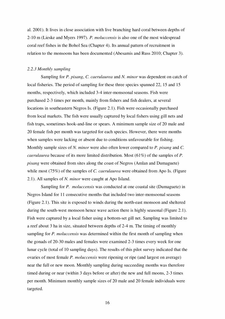
2.2.3 Monthly sampling
Sampling for P. pisang, C. caerulaurea and N. minor was dependent on catch of
local fisheries. The period of sampling for these three species spanned 22, 15 and 15
months, respectively, which included 3-4 inter-monsoonal seasons. Fish were
purchased 2-3 times per month, mainly from fishers and fish dealers, at several
locations in southeastern Negros Is. (Figure 2.1). Fish were occasionally purchased
from local markets. The fish were usually captured by local fishers using gill nets and
fish traps, sometimes hook-and-line or spears. A minimum sample size of 20 male and
20 female fish per month was targeted for each species. However, there were months
when samples were lacking or absent due to conditions unfavourable for fishing.
Monthly sample sizes of N. minor were also often lower compared to P. pisang and C.
caerulaurea because of its more limited distribution. Most (61%) of the samples of P.
pisang were obtained from sites along the coast of Negros (Amlan and Dumaguete)
while most (75%) of the samples of C. caerulaurea were obtained from Apo Is. (Figure
2.1). All samples of N. minor were caught at Apo Island.
Sampling for P. moluccensis was conducted at one coastal site (Dumaguete) in
Negros Island for 11 consecutive months that included two inter-monsoonal seasons
(Figure 2.1). This site is exposed to winds during the north-east monsoon and sheltered
during the south-west monsoon hence wave action there is highly seasonal (Figure 2.1).
Fish were captured by a local fisher using a bottom-set gill net. Sampling was limited to
a reef about 3 ha in size, situated between depths of 2-4 m. The timing of monthly
sampling for P. moluccensis was determined within the first month of sampling when
the gonads of 20-30 males and females were examined 2-3 times every week for one
lunar cycle (total of 10 sampling days). The results of this pilot survey indicated that the
ovaries of most female P. moluccensis were ripening or ripe (and largest on average)
near the full or new moon. Monthly sampling during succeeding months was therefore
timed during or near (within 3 days before or after) the new and full moons, 2-3 times
per month. Minimum monthly sample sizes of 20 male and 20 female individuals were
targeted.

17
2.2.4 Macroscopic examination of gonads
Fish were kept in ice soon after capture and dissected in the laboratory within
24-36 hours of capture. Before dissection, the total, fork and/or standard body lengths
(whichever were most appropriate for the species) of each fish were measured to the
nearest mm. Whole body weight was measured to the nearest 0.1 g using an electronic
balance. The gonads of each fish were then examined to determine sex and estimate
gonad maturity stage. A five-point (Stages I-V) macroscopic gonad staging scale was
developed for each species during the early part of monthly sampling. This gonad
staging scale was modified from the scheme proposed by (Holden and Raitt 1974) for
partial spawners (Table 2.2). This scheme was used because the four species were
assumed to have asynchronous development of gametes (oocytes) and protracted
periods of spawning at lower latitudes. Gonads of immature fish were classified into
Stage I. Classification of gonads of a sexually-mature fish into Stage II (Resting)
indicated that the fish would not spawn and gonads were ‘inactive’. Classification of
gonads into Stage III (Ripening), IV (Ripe) and V (Spent), on the other hand, indicated
that spawning of the fish was imminent or had occurred recently and the gonads were
‘active’.
A gonadosomatic index (GSI) was also calculated for each female fish to
provide a supplementary indicator of gonad maturity. Ovaries were dissected from the
fish then weighed to the nearest 0.001 g using an electronic balance. GSI was calculated
using the equation:
%100×=b
g
W
WGSI (Equation 2.1),
where Wg is the gonad weight and Wb is the whole body weight.
Sex ratios (male : female) were calculated for each species using only sexually-
mature individuals (i.e., operational sex ratio). A chi-squared test (α = 0.05) (Zar 1999)
was used to test for significant deviation from an expected sex ratio of 1 male : 1
female.
2.2.5 Histological examination of ovaries
Subsamples of ovaries classified into Stages II, III, IV and V were obtained
during the first half of the sampling period of each species. These were fixed in 10%

18
External appearance
Stage Ovary Testis
A. Pterocaesio pisang and Caesio caerulaurea
I-Immature - Difficult to distinguish sex; gonads are small, elongated or ribbon-like; light pink or translucent
II-Resting - Small, cylindrical; pink; oocytes not visible - Small, flat; whitish; milt not present
III-Ripening - Larger, cylindrical, more firm; yellowish-pink;
blood vessels visible; oocytes becoming visible
- Larger, thicker; white; exudes milt when
cut but not when pressed
IV-Ripe - Very large, full; yellow-pink to orange; oocytes
are visible, may be extruded with slight touch
- Large, very thick, wrapped around
intestine; creamy white; exudes milt when
pressed
V-Spent - Flaccid, with ‘loose’ walls; reddish orange to
dark pink; oocytes visible in some ‘spent’ ovaries
- Shrunken and flaccid; reddish to pinkish-
white; milt may be present
B. Naso minor
I-Immature - Not seen
II-Resting - Small, lobe-shaped but not flat; pink; oocytes
not visible
- Small, lobe-shaped, flat; pinkish-white;
milt not present
III-Ripening - Larger, more cylindrical in appearance; pink;
blood vessels visible; oocytes becoming visible
- Larger, still relatively flat but thicker;
exudes milt when cut but not when
pressed
IV-Ripe - Large and full, very soft; pink; oocytes plainly
visible and may be extruded with slight touch
- Larger, fuller; readily exudes milt when
pressed
V-Spent - Not seen
- Flaccid; pinkish; milt may be present;
difficult to distinguish from Stage II
C. Pomacentrus moluccensis
I-Immature - Difficult to distinguish sex; gonads are very small and thread-like; translucent
II-Resting - Very small, oval-shaped; pink to dark pink;
oocytes not visible
- Very small, thread-like; whitish; milt not
present
III-Ripening - Larger, fuller, oval to irregular shape; pinkish
orange; oocytes becoming visible
- Larger but not very thick; whitish; milt
present
IV-Ripe - Large and full, irregular shape; orange; oocytes
plainly visible
- Larger; whitish to white; milt freely flowing
V-Spent - Appears shrunken, soft, with ‘loose’ walls; dark
pink
- Shrunken, flaccid; pinkish-white; milt
sometimes present
Table 2.2 Maturity stages of gonads of Pterocaesio pisang, Caesio caerulaurea, Naso minor and Pomacentrus moluccensis. Descriptions of external appearance of the ovary and testis were based on the scheme proposed by Holden and Raitt (1974) for partial (heterochronal) spawners. Gonads of sexually mature individuals are considered ‘inactive’ at Stage II and ‘active’ at Stages III, IV and V.

19
formalin for 7-10 days then transferred to 75% ethanol. Ovaries were prepared for
histology following conventional procedures of dehydrating, embedding, sectioning and
staining with hematoxylin and eosin. Between 25-50 transverse sections (depending on
the size of the ovary) ~7 µm thick were obtained through the mid-section of each ovary.
The histological sections were then examined microscopically to assess the accuracy of
staging whole ovaries. Under microscopic examination, the most advanced oocyte
stages that should be present in Stage II, III and IV ovaries should be as follows: Stage
II – previtellogenic oocytes (i.e., chromatin nucleolar, perinucleolar to germinal vesicle
stages); Stage III – vitellogenic oocytes (i.e., yolk globule stages); Stage IV – ripe
oocytes (i.e., migratory nucleus and hydrated oocyte stages). Stage V ovaries (‘spent’)
were expected to have post-ovulatory follicles. Classification into the different Stages
was based on the presence of the most advanced oocyte that was expected for a
particular stage, not on quantitative criterion based on the relative frequencies of
oocytes stages. Identification of the different oocyte stages and other histological
features of the ovary were based on West (1990), Ganias et al. (2004) and Choi et al.
(1996). Correction factors based on the relative frequency (%) of correct and incorrect
classification (macroscopic versus histological examination) of the subsamples per
ovary maturity stage (Results, Table 2.3) were applied to the larger data set on
macroscopic classification of ovaries to improve accuracy of gonad staging.
2.2.6 Examination of temporal patterns of spawning
For each species, the monthly relative frequency of individuals in the different
gonad maturity stages and the monthly average female GSI were examined in relation
to monsoon and inter-monsoonal periods to determine any seasonal pattern. Gonad
maturation patterns were also compared to available data on monthly average sea
surface temperature (SST) and monthly total rainfall for the study area. Absolute and
relative changes in temperature are often implicated as an important factor in the
spawning of reef fishes (Munro et al. 1973; Sadovy 1996) and the growth and survival
of their larvae (Bergenius et al. 2002; Meekan et al. 2003). Rainy periods, on the other
hand, may be associated with increased availability of planktonic food (due to nutrient
input into coastal waters by terrestrial runoff), which could result in increased spawning
activity for planktivorous fishes (Tyler and Stanton 1995) and better survival of larvae
(Gallego et al. 1996). Data on SST were obtained from the NOAA Coral Reef Watch
Program (http://coralreefwatch.noaa.gov/satellite/index.html) which archives SST data

20
measured by a ‘virtual’ monitoring station (0.5º longitude x 0.5º latitude in area) in the
vicinity of the study area (Figure 2.1). The temporal resolution of this data was bi-
weekly, giving 7-8 measurements per month for each monthly average value. Daily
data on rainfall was obtained from a weather station in Negros (Dumaguete) that is
operated by the PAGASA. This weather station is located almost at sea level < 1 km
from the coast (Figure 2.1). The monthly pattern of total rainfall reflected major rainy
periods due to the inter-tropical convergence zone and occasional typhoons, as opposed
to just localized rain in the Dumaguete area. The gonad maturation patterns of
Pomacentrus moluccensis were further compared to data on monthly average wind
speed obtained from daily wind data recorded by the PAGASA weather station. The
sampling site for P. moluccensis was located < 1km away from this weather station.
Data on wind speed was used as a proxy for wind stress, which causes seasonality of
wave action in the site where P. moluccensis was sampled.
Spearman rank correlation (rs) (Zar 1999) was used to assess synchrony
between monthly proportions of individuals with active testes, active ovaries and
monthly average GSI. The same statistical procedure was used to determine the
relationships between each of these indicators of gonad maturation versus each of the
environmental variables of interest.
2.2.7 Estimation of batch fecundity
For each species, a subsample (n = 13-14) of ovaries classified as Stage IV
(Ripe) was preserved in 10% formalin. Estimates of batch fecundity (number of eggs
per spawning) were obtained from these ovaries using the gravimetric (or hydrated
oocyte) method developed by Hunter et al. (1985) for multiple spawners. This method
uses counts of hydrated oocytes per replicate subsample of ovary tissue of known
weight. The counts are then extrapolated to the total weight of the ovary to estimate the
total number of hydrated eggs that would have comprised a spawning batch. When
hydrated oocytes were not present in the subsample (e.g., in all P. moluccensis and
some P. pisang and C. caerulaurea), the largest yolked oocytes were counted because it
can be assumed that these oocytes would have comprised a single batch of eggs in one
spawning (Hunter et al. 1985). In P. pisang and C. caerulaurea, the largest yolked
oocytes (and their abundance) in a given subsample were determined by constructing a
size-frequency histogram based on oocyte diameters (Hunter et al. 1985). To determine
if counts of hydrated (or largest) oocytes differed between lobes and among regions of
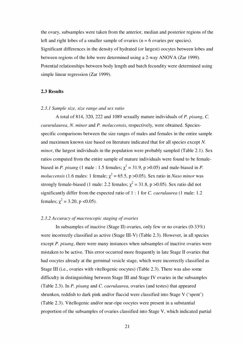
21
the ovary, subsamples were taken from the anterior, median and posterior regions of the
left and right lobes of a smaller sample of ovaries (n = 6 ovaries per species).
Significant differences in the density of hydrated (or largest) oocytes between lobes and
between regions of the lobe were determined using a 2-way ANOVA (Zar 1999).
Potential relationships between body length and batch fecundity were determined using
simple linear regression (Zar 1999).
2.3 Results
2.3.1 Sample size, size range and sex ratio
A total of 814, 320, 222 and 1089 sexually mature individuals of P. pisang, C.
caeurulaurea, N. minor and P. moluccensis, respectively, were obtained. Species-
specific comparisons between the size ranges of males and females in the entire sample
and maximum known size based on literature indicated that for all species except N.
minor, the largest individuals in the population were probably sampled (Table 2.1). Sex
ratios computed from the entire sample of mature individuals were found to be female-
biased in P. pisang (1 male : 1.5 females; χ2 = 31.9, p >0.05) and male-biased in P.
moluccensis (1.6 males: 1 female; χ2 = 65.5, p >0.05). Sex ratio in Naso minor was
strongly female-biased (1 male: 2.2 females; χ2 = 31.8, p >0.05). Sex ratio did not
significantly differ from the expected ratio of 1 : 1 for C. caerulaurea (1 male: 1.2
females; χ2 = 3.20, p <0.05).
2.3.2 Accuracy of macroscopic staging of ovaries
In subsamples of inactive (Stage II) ovaries, only few or no ovaries (0-33%)
were incorrectly classified as active (Stage III-V) (Table 2.3). However, in all species
except P. pisang, there were many instances when subsamples of inactive ovaries were
mistaken to be active. This error occurred more frequently in late Stage II ovaries that
had oocytes already at the germinal vesicle stage, which were incorrectly classified as
Stage III (i.e., ovaries with vitellogenic oocytes) (Table 2.3). There was also some
difficulty in distinguishing between Stage III and Stage IV ovaries in the subsamples
(Table 2.3). In P. pisang and C. caerulaurea, ovaries (and testes) that appeared
shrunken, reddish to dark pink and/or flaccid were classified into Stage V (‘spent’)
(Table 2.3). Vitellogenic and/or near-ripe oocytes were present in a substantial
proportion of the subsamples of ovaries classified into Stage V, which indicated partial

22
Ovary
maturity stage
n
Correct
Incorrect
A. Pterocaesio pisang
II-Resting 11 10 (90.9) 1 (9.1) - 1º yolk globule stage (early III)
III-Ripening 9 6 (66.7) 2 (22.2)
1 (11.1)
- migratory nucleus stage (IV)
- perinucleolar stage (II)
IV-Ripe 21 10 (47.6) 10 (47.6)
1 (4.8)
- 3º yolk globule stage (late III)
- germinal vesicle stage (II)
V-Spent 8 1 (12.5) 6 (75.0)
1 (12.5)
- 3º yolk globule stage (III)
- migratory nucleus stage (IV)
B. Caesio caerulaurea
II-Resting 13 12 (92.3) 1 (7.7) - 1º yolk globule stage (early III)
III-Ripening 8 1 (12.5) 7 (87.5) - germinal vesicle stage (late II)
IV-Ripe 17 10 (58.8) 7 (41.2) - 3º yolk globule stage (late III)
V-Spent
6 2 (33.3) 3 (50.0)
1 (16.7)
- 1º-3º yolk globule stages (III)
- germinal vesicle stage (II)
C. Naso minor
II-Resting 3 2 (66.7) 1 (33.3) - 3º yolk globule stage (late III)
III-Ripening 16 8 (50.0) 8 (50.0) - germinal vesicle stage (late II)
IV-Ripe 12 6 (50.0) 5 (41.7)
1 (8.3)
- 3º yolk globule stage (late III)
- perinucleolar stage (II)
V-Spent - - - -
D. Pomacentrus moluccensis
II-Resting 14 14 (100.0) - -
III-Ripening 16 8 (50.0) 8 (50.0) - perinucleolar to germinal vesicle stage (II)
IV-Ripe 18 4 (22.2) 14 (77.7) - 2º-3º yolk globule stages (late III)
V-Spent - - - -
Table 2.3 Results of microscopic examination of ovaries to assess the accuracy of estimating maturity stage based on external appearance. Percent of correctly and incorrectly classified ovaries per ovary maturity stage are given in parentheses. The latest oocyte stage (and gonad maturity stage, in parentheses) and other features seen in incorrectly classified ovaries are also indicated. Gonads of sexually mature individuals are considered ‘inactive’ at Stage II and ‘active’ at Stages III, IV and V.

23
spawning in these species. These results became the basis for correction factors that
were applied to the data on macroscopic classification of ovaries of each species.
2.3.3 Temporal patterns of spawning
In P. pisang, active testes and ovaries were present during every month that was
sampled (Figures 2.2c,d). Stage V (‘spent’) testes and ovaries were also present during
many months. A higher percentage of individuals had active gonads during the first
inter-monsoonal season (March-June 2008) and the second north-east monsoon season
extending to the third inter-monsoonal monsoon season (November 2008-May 2009) of
the period that was sampled (Figure 2.2c,d). Average GSI of females also peaked
within these seasons, in May 2008 and January 2009 (Figure 2.2e). Peaks in gonad
maturation and GSI occurred within 2-3 days before or after the new moon or the full
moon (Figure 2.2). Correlations between the monthly percent frequency of active testes,
active ovaries and monthly GSI were moderate to high (Table 2.4). There was no clear
relationship between the pattern of gonad maturation and fluctuations in SST (Figure
2.2a,c-e). SST was increasing or decreasing to lowest levels as percent frequency of
active gonads and average GSI reached peak levels, but monthly percent frequency of
active gonads and average GSI were low when SST was highest (during the south-west
monsoon season). There was, however, some indication that the seasonal pattern of
gonad maturation was tracking the pattern of rainfall (Figure 2.2b-e). Gonad maturation
patterns had a weak negative correlation with SST and a weak positive correlation with
rainfall, but these relationships were only statistically significant for GSI (Table 2.4).
In C. caerulaurea, active testes and ovaries were also present during all months
sampled. The percent frequency of active testes was higher during a 9-month period
that encompassed consecutive south-west monsoon, inter-monsoon and north-east
monsoon seasons (July 2008 to March 2009) (Figure 2.3c). Stage IV (ripe) testes were
more frequent in the first 5 months of this period (south-west monsoon to early north-
east monsoon season). The frequency of active ovaries was also usually higher during
this 9-month period but peaks occurred during the south-west monsoon and inter-
monsoonal seasons (August and October 2008) (Figure 2.3d). Average GSI of females
peaked during the south-west monsoon (August 2008) (Figure 2.3e). There was some
indication that percent frequency of active ovaries and average GSI were higher near
the new moon (Figure 2.3). Correlations of monthly frequency of active testes versus
frequency of active ovaries and average female GSI were low to negligible, but high

24
Figure 2.2 Monthly gonad maturation patterns of Pterocaesio pisang versus environmental variables: average monthly sea surface temperature (SST) (a); total monthly rainfall (b); relative frequency of individuals in different gonad maturity stages for males (c) and females (d); average monthly female GSI (e). Legend for (c) and (d): Stage II (Resting) – white; Stage III (Ripening) – grey; Stage IV (Ripe) – black; Stage V (Spent) – diagonal lines. Numbers on top of bars in (c) and (d) indicate sample size. Monsoons (seasonal wind regime) and inter-monsoonal periods are indicated by different shades of grey on the bar at the bottom of the figure, parallel to the x-axis (months): NE – north-east monsoon, SW – south-west monsoon, I – inter-monsoon. If more than 50% of the samples in a particular month were caught within 2 days before or after the day of the new moon or full moon, a black circle (for new moon) or white circle (for full moon) is indicated under the letter representing that month.
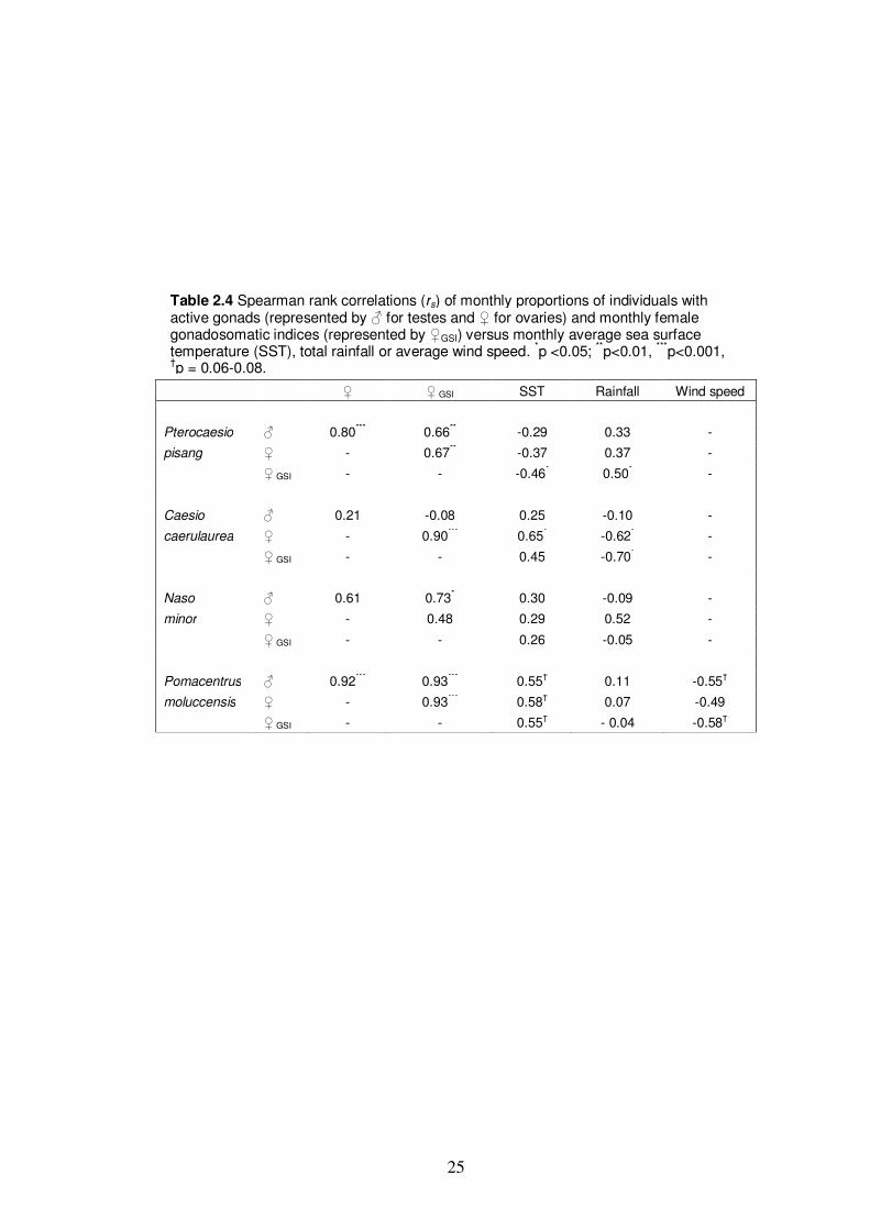
25
♀ ♀ GSI SST Rainfall Wind speed
Pterocaesio ♂ 0.80***
0.66** -0.29 0.33 -
pisang ♀ - 0.67** -0.37 0.37 -
♀ GSI - - -0.46* 0.50
* -
Caesio ♂ 0.21 -0.08 0.25 -0.10 -
caerulaurea ♀ - 0.90***
0.65* -0.62
* -
♀ GSI - - 0.45 -0.70* -
Naso ♂ 0.61 0.73* 0.30 -0.09 -
minor ♀ - 0.48 0.29 0.52 -
♀ GSI - - 0.26 -0.05 -
Pomacentrus ♂ 0.92***
0.93***
0.55† 0.11 -0.55
†
moluccensis ♀ - 0.93***
0.58† 0.07 -0.49
♀ GSI - - 0.55† - 0.04 -0.58
†
Table 2.4 Spearman rank correlations (rs) of monthly proportions of individuals with active gonads (represented by ♂ for testes and ♀ for ovaries) and monthly female gonadosomatic indices (represented by ♀GSI) versus monthly average sea surface temperature (SST), total rainfall or average wind speed.
*p <0.05;
**p<0.01,
***p<0.001,
†p = 0.06-0.08.

26
between monthly frequency of active ovaries and GSI (Table 2.4). Patterns of gonad
maturation had a tendency to be positively correlated with SST and negatively
correlated with rainfall (Table 2.4). The correlations of maturation of ovaries and
female GSI with these environmental variables were stronger and more often
statistically significant (Table 2.4).
The annual pattern of gonad maturation in N. minor was difficult to discern
due to lack of samples during several months (Figure 2.4). The available data, however,
suggested that active ovaries were present in all months that were sampled. Active
testes were present during most months. Percent frequency of active ovaries and
average GSI were usually higher near the new moon (Figure 2.4). There was some
suggestion of higher frequency of active ovaries during the earlier part of the second
north-east monsoon season (November-December 2008) (Figure 2.4). Outside of this
season, active testes were absent or less frequent (March, May and September 2008).
Differences in the frequencies of active gonads and average female GSI between north-
east monsoon and inter-monsoonal seasons were not apparent (Figure 2.4). Correlations
between monthly percent frequency of active testes, active ovaries and monthly GSI
were low to moderate (Table 2.4). Maturation of testes, ovaries and average GSI had
weak positive relationships with SST but none of these relationships were statistically
significant. Correlations between gonad maturation patterns and rainfall were negligible
except for frequency of active ovaries which had a positive (but not statistically
significant) relationship with rainfall.
In P. moluccensis, a strong seasonal pattern was detected in the maturation of
testes and ovaries and the fluctuations in female GSI (Figure 2.5). The percent
frequency of active gonads and average GSI were much higher during the south-west
monsoon and inter-monsoonal seasons (Figure 2.5c-e). Conversely, the percent
frequency of inactive gonads and average GSI were lowest from December to January,
during the north-east monsoon. The inferred seasonal pattern of spawning appeared to
be directly proportional to SST and inversely related to wind speed. Strong correlations
were detected between the patterns of maturation of testes and ovaries and the patterns
of GSI (Table 2.4). Gonad maturation and GSI had moderate positive relationships with
SST and moderate negative relationships with wind speed, but these were not
statistically significant (p ranged from 0.06 to 0.08). Correlations between gonad
maturation and GSI versus rainfall were negligible (Table 2.4).

27
Figure 2.3 Monthly gonad maturation patterns of Caesio caerulaurea versus environmental variables. Labels and legends are the same as in Figure 2.2.

28
Figure 2.4 Monthly gonad maturation patterns of Naso minor versus environmental variables. Labels and legends are the same as in Figure 2.2.

29
2.3.4 Estimates of batch fecundity
No significant differences in the density of hydrated (or largest) oocytes
(number of hydrated oocytes per gram ovary tissue) were found among the regions of
the lobes (i.e., anterior, median and posterior) and between the lobes of the ovaries of
C. caerulaurea, N. minor and P. moluccensis (Table 2.5). In P. pisang, however, a
significant difference was detected between regions, but not between lobes (Table 2.5).
There was a decreasing trend in the density of oocytes from the anterior to the posterior
region of the ovaries of P. pisang. A post-hoc test (Tukey’s test) indicated that oocyte
density was significantly higher (by 23%) in the anterior region than in the posterior
region. For each species, batch fecundity was estimated using counts of hydrated (or
largest) oocytes taken from 3 replicate subsamples of ovary tissue, one each from the
anterior, median and posterior regions, of a randomly selected lobe of the ovary.
Estimates of average batch fecundity per species are given in Table 2.6. Batch
fecundity was highest in the largest species, C. caerulaurea and lowest in the smallest
one, P. moluccensis. Batch fecundity was more variable in C. caerulaurea and N. minor
and less variable in P. moluccensis and P. pisang (Table 2.6). Batch fecundity was
found to increase with size in the two species of fusilier, but this relationship was weak
(and not statistically significant) in P. pisang. Batch fecundity and body size had no
apparent relationship in N. minor and P. moluccensis within the ranges of size that were
examined. However, the size range that was examined for each species was small
(Table 2.6).
2.4 Discussion
The expectation of protracted breeding seasons of coral reef fishes at lower
latitudes was confirmed. The gonads of all four species were in spawning condition
almost every month that was sampled. Broad spawning peaks were evident. However,
the timing of inferred spawning peaks in relation to the monsoons varied between
species. Only P. pisang showed a spawning peak in one year that coincided with the
longer inter-monsoonal period of the year – a pattern that is consistent with the findings
of Cabanban (1984) for this species in the same area. In the following year, the
spawning peak of P. pisang occurred during the north-east monsoon and may have
extended to the succeeding inter-monsoonal period. In C. caerulaurea, a probable
spawning peak occurred during the south-west monsoon and the following (shorter)
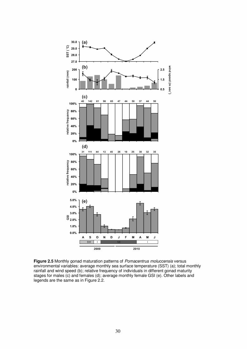
30
Figure 2.5 Monthly gonad maturation patterns of Pomacentrus moluccensis versus environmental variables: average monthly sea surface temperature (SST) (a); total monthly rainfall and wind speed (b); relative frequency of individuals in different gonad maturity stages for males (c) and females (d); average monthly female GSI (e). Other labels and legends are the same as in Figure 2.2.
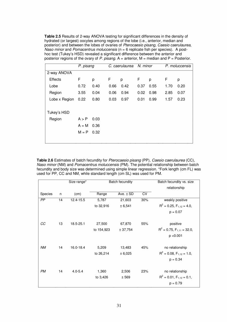
31
P. pisang C. caerulaurea N. minor P. moluccensis
2-way ANOVA
Effects F p F p F p F p
Lobe 0.72 0.40 0.66 0.42 0.37 0.55 1.70 0.20
Region 3.55 0.04 0.06 0.94 0.02 0.98 2.85 0.07
Lobe x Region 0.22 0.80 0.03 0.97 0.01 0.99 1.57 0.23
Tukey’s HSD
Region A > P 0.03
A = M 0.36
M = P 0.32
Size range* Batch fecundity Batch fecundity vs. size
relationship
Species n (cm) Range Ave. ± SD CV
PP 14 12.4-15.5 5,787
to 32,916
21,603
± 6,541
30% weakly positive
R2 = 0.25, F1,12 = 4.0,
p = 0.07
CC 13 18.5-25.1 27,500
to 154,923
67,870
± 37,754
55% positive
R2 = 0.75, F1,11 = 32.0,
p <0.001
NM 14 16.0-18.4 5,209
to 26,214
13,483
± 6,025
45% no relationship
R2 = 0.08, F1,12 = 1.0,
p = 0.34
PM 14 4.0-5.4 1,360
to 3,426
2,506
± 569
23% no relationship
R2 = 0.01, F1,12 = 0.1,
p = 0.79
Table 2.5 Results of 2-way ANOVA testing for significant differences in the density of hydrated (or largest) oocytes among regions of the lobe (i.e., anterior, median and posterior) and between the lobes of ovaries of Pterocaesio pisang, Caesio caerulaurea, Naso minor and Pomacentrus moluccensis (n = 6 replicate fish per species). A post-hoc test (Tukey’s HSD) revealed a significant difference between the anterior and posterior regions of the ovary of P. pisang. A = anterior, M = median and P = Posterior.
Table 2.6 Estimates of batch fecundity for Pterocaesio pisang (PP), Caesio caerulaurea (CC), Naso minor (NM) and Pomacentrus moluccensis (PM). The potential relationship between batch fecundity and body size was determined using simple linear regression. *Fork length (cm FL) was used for PP, CC and NM, while standard length (cm SL) was used for PM.
32
inter-monsoonal period. The annual pattern of spawning was less clear in N. minor, but
there was a weak indication of spawning activity being slightly higher during the north-
east monsoon. In P. moluccensis, spawning activity was high throughout the year
except during the north-east monsoon. Taken together, these results do not provide
strong support for the notion that the timing of reproduction in reef fishes in monsoonal
environments tracks the inter-monsoonal periods.
If the timing of spawning of reef fishes in the area that was studied has adapted
to take advantage of optimum conditions for survival of larvae, then the results indicate
that such conditions are not restricted to the inter-monsoonal periods. A study on
recruitment of reef fishes in the same locality partly supports this suggestion. Abesamis
and Russ (2010) (Chapter 3) showed that for many species, the best ‘window’ for
recruitment is during a period of 4-6 consecutive months that includes the two inter-
monsoonal periods and the south-west monsoon (May to October). They concluded that
warmer temperatures and weaker winds (locally) during this recruitment window are
critical to larval survival. However, assuming that the same 4-6 month period is
important for the larvae of all four species considered here, it would appear that only C.
caerulaurea and P. moluccensis have adapted to take advantage of this period. Note
that a reasonable case for adaptation can be made for P. moluccensis since this species
dominated recruit densities in the study by Abesamis and Russ (2010) (but alternative
explanations for the seasonal pattern of spawning in this species are given below).
Other conditions beneficial to larvae that occur outside of the inter-monsoonal
periods are possible, which may explain the patterns of spawning in the other two
species, particularly P. pisang. For instance, the monsoons may result in regional or
local upwelling depending on the degree of exposure and orientation of a site to
prevailing winds (Wang et al. 2006, Cabrera et al. 2011, Villanoy et al. 2011).
McIlwain et al. (2006) found that four demersal species of fish in Oman (Arabian Sea)
appeared to match their spawning with the south-west monsoon. They hypothesised that
the timing of spawning in these four species maximizes larval survivorship due to the
increased primary productivity brought by upwelling (McIlwain et al. 2006). Such a
possibility would further weaken the argument for the importance of inter-monsoonal
periods and complicate the detection of an adaptive response of reef fishes to
favourable conditions for their larvae. Clearly, the potential effects of the monsoons on
survival of reef fish larvae warrant further investigation.
33
Alternatively, the patterns of spawning described here possibly reflect
temperature, rainfall, wind or wave action more directly affecting the spawning of
adults, as opposed to adaptation of reproduction to ensure higher survivorship of larvae
in the pelagic environment. Potential relationships between spawning and
environmental variables were evident in P. pisang, C. caerulaurea and P. moluccensis.
The nature of these relationships varied among species, which suggests that responses
of adults were species- and/or location-specific. The relationship between
environmental factors and spawning in N. minor, however, requires further study.
The results indicate that temperature and rainfall were correlated in opposite
ways to the temporal pattern of spawning in the two more closely-related species, the
fusiliers P. pisang, and C. caerulaurea. At first glance, these results are difficult to
explain. However, a closer examination shows that the first peak of spawning of P.
pisang occurred when SST was increasing. Similarly, the peak of spawning of C.
caerulaurea was positively correlated with SST. Increasing temperatures may therefore
be an important cue for spawning in fusiliers. This assertion is supported by previous
studies on reproduction in fusiliers. The spawning season of C. caerulaurea in
Okinawa, Japan (26º N) coincides with increasing temperatures around June
(Yokoyama et al. 1995). Another species of fusilier, Pterocaesio digramma, also has a
spawning period that occurs around the same time of year in the same locality
(Yokoyama et al. 1994; Choi et al. 1996). The annual pattern of spawning in P. pisang
previously documented by Cabanban (1984) at two offshore sites in the Bohol Sea
(Apo and Sumilon Is.) could then be due to increasing temperatures from February to
June.
In the present study, a second spawning peak in P. pisang occurred when
temperature was decreasing, suggesting the influence of other environmental factors.
Results point to food availability driven by rainfall as a factor that is likely to affect
spawning activity in P. pisang. The spawning of this species had a weak but statistically
significant positive correlation with rainfall. Abundance of plankton in tropical areas
can vary seasonally with rainfall because the latter usually increases terrestrial run-off
and nutrient input into coastal areas (Sander and Steven 1974; Grahame 1976;
Sammarco and Crenshaw 1984). Spawning activity has been positively correlated with
freshwater discharge in coastal populations of a planktivorous reef fish (Abudefduf
abdominalis) in Hawaii (Tyler and Stanton 1995). Furthermore, food availability has a
direct relationship with reproductive activity in reef fishes (Clifton 1995; Tyler and

34
Stanton 1995). In the present study, rainfall may have had an indirect positive influence
on the pattern of spawning of P. pisang but a similar situation was not apparent in C.
caerulaurea (a negative correlation between rainfall and spawning was detected). This
discrepancy may be partly explained by geographic location, i.e., degree of exposure of
sampling sites to major sources of terrestrial run-off. The majority (61%) of the P.
pisang samples came from sites along the coast of Negros (Amlan and Dumaguete,
Figure 2.1), closer to several rivers and many streams. On the other hand, the majority
(75%) of the C. caerulaurea samples came from an offshore site (Apo Is.) 7 km away
from the nearest coast. However, degree of exposure to terrestrial run-off cannot
explain the negative correlation between rainfall and spawning activity in C.
caerulaurea. Future studies should attempt to measure spawning activity of
planktivorous reef fishes at different sites and relate the information to data on
concentrations of planktonic prey, rainfall, freshwater discharge, and other factors such
as monsoon-induced upwelling.
In P. moluccensis, the depression of spawning activity during the north-east
monsoon may have been a direct or indirect consequence of environmental stresses
specific (but not unique) to the site where this species was studied. Spawning was
negatively correlated with wind but positively correlated with temperature (both not
significant statistically), suggesting three possible mechanisms driving the annual
pattern of spawning. First, heavy wave action due to north-east monsoon winds may
make nesting difficult or disadvantageous for P. moluccensis, especially in shallower
water. A similar point was made by Robertson (1990) to explain the lower spawning
output of two species of damselfish (Stegastes partitus and S. diencaeus) at a Caribbean
site in San Blas, Panama during periods when that site was exposed to heavy wave
action brought by the dry season tradewind. The second potential mechanism is related
to the first. Heavy wave action during the north-east monsoon may result in lower
abundance of the benthic algae that is eaten by P. moluccensis, resulting in decreased
reproductive output or failure to store enough energy reserves for spawning. This type
of mechanism involving food limitation was demonstrated convincingly by Clifton
(1995) in an herbivorous reef fish (the parrotfish Scarus iserti) at two Caribbean sites in
San Blas that differed in their exposures to the dry season tradewind. In the exposed
reef that Clifton studied, strong wave action may have reduced algal food levels directly
by physical removal or indirectly by decreasing water clarity (increasing turbidity). The
third mechanism could be related to lower temperatures during the north-east monsoon.
35
For instance, Robertson (1990) showed that the spawning output of two species of
damselfish (Stegastes acapulcoensis, S. flavilatus) at a Pacific site in Panama was lower
during periods when temperature was lower. However, the drop in temperature at that
Panamanian site is considerable (from average of 30 ºC to just 14-18 ºC) due to local
upwelling, which casts some doubt about the importance of temperature in the pattern
of spawning of P. moluccensis in the present study (annual temperature difference in
the Dumaguete site is < 3 ºC). Future studies on the reproduction of P. moluccensis and
other shallow-water reef fishes in monsoonal environments should investigate these
three potential mechanisms. A comparative approach would be most useful, wherein
populations subject to different degrees of exposure to the two monsoons are sampled.
The protracted spawning seasons described in this study may be typical of
smaller-bodied species of reef fish. For instance, in her review of the temporal patterns
of spawning of reef fishery species, Sadovy (1996, p. 35-36) found an inverse
relationship between body size and duration of spawning season among species within
three families (i.e., groupers, emperors and snappers). Robertson (1990) argued that
smaller-bodied species may be limited by shorter lifespans and low capacity to store
resources for future egg production, which could prevent a strategy of timing spawning
peaks to coincide with periods that would favour survivorship of larvae. Comparative
studies on the patterns of reproduction between smaller- and larger-bodied species of
reef fish in relation to the monsoons are required to elucidate size-related temporal
spawning strategies.
The possible influence of lunar patterns of spawning on the inferred annual
patterns of spawning in P. pisang, C. caerulaurea and N. minor deserves a brief
discussion. There were indications that the percent frequency of active ovaries and
average GSI were higher around the full moon and new moon for P. pisang, and around
the new moon for C. caerulaurea and N. minor (Figures 2.2-2.4). However, gonad
maturation patterns in the two species of fusilier did not have a predictable relationship
with the lunar cycle. For instance, in P. pisang, the frequency of active ovaries and
average GSI were low around the time of the full moon during several months
(February 2008, July 2009 and September 2009) (Figure 2.2). For C. caerulaurea, the
highest average GSI, which was recorded in August 2008, did not occur around the
time of the new moon (Figure 2.3). Furthermore, daily observations by Yokoyama et al.
(1994, 1995) on the reproductive behaviour of two species of fusilier (P. digramma and
C. caerulaurea) suggested that spawning in fusiliers is not associated with the lunar
36
cycle. Thus, in the present study, the inferred annual patterns of spawning of P. pisang
and C. caerulaurea were probably not indicative of lunar patterns of spawning. On the
other hand, the possible influence of the lunar cycle on the inferred annual pattern of
spawning in N. minor cannot be ruled out. No studies on the lunar patterns of spawning
of N. minor are available.
In conclusion, the monsoons may play an important role in the timing of
reproduction of reef fishes, but it is clear from this study that peaks in spawning activity
are not necessarily restricted to the inter-monsoonal periods. The influence of the
monsoons on spawning seasonality is likely to be complex. Many environmental
variables change with the monsoons. These variables also vary at several spatial scales.
Although it cannot be denied that some species appear to take advantage of inter-
monsoonal conditions presumably to increase survivorship of larvae (Johannes 1978),
the effect of the monsoons on reproduction is obviously not uniform across all species.
However, the lack of a consistent pattern between species may also be partly due to the
limited number of species that were examined and the limited time of the study, which
did not allow the documentation of inter-annual variability. We still know very little
about the annual patterns of spawning of reef fishes in monsoonal environments and
how important these patterns are in the dynamics of reef fish populations. Protracted
spawning periods are likely to be typical of reef fishes situated at lower latitudes
(Robertson 1991) but the ways in which the monsoons may influence the spatial and
temporal patterns of reproduction and recruitment in reef fishes warrant further
investigation.

37
Chapter 3
Patterns of recruitment of coral reef fishes
in a monsoonal environment*
Abstract. The abundance of newly settled recruits of coral reef fishes was monitored at
a total of 11 sites at two islands and two coastal locations in the central Philippines for a
20-month period (February 2008 to September 2009) that included two monsoon
cycles. Recruitment occurred throughout the year. Most of the abundant species
exhibited protracted recruitment seasons. This confirms the expectation of extended
breeding of reef fishes at lower latitudes (see Chapter 2). The annual pattern of
recruitment of reef fishes as a group was reasonably predictable. Annual fluctuations of
sea surface temperature and wind strength largely explained the pattern. Rainfall,
however, did not significantly influence the pattern of recruitment. Peaks in density and
species richness of recruits occurred during the southwest monsoon and the second
inter-monsoonal period of the year (July to October) when temperatures were highest
and when most of the sites were sheltered from winds or when winds were weak.
Conversely, lowest density and species richness of recruits were observed during the
northeast monsoon (November to March) when temperatures were lowest and most
sites were exposed to winds. The same pattern could also be seen in the recruitment of
both damselfishes (Pomacentridae) and wrasses (Labridae), notwithstanding a 10-fold
difference in abundance of recruits between the two families. The pattern was fairly
consistent across most sites, among most of the species that were examined, and
between the two years that were sampled. This study is one of the few to provide
insights into the influence of environmental factors on the recruitment patterns of fishes
on Indo-Pacific coral reefs situated at lower latitudes.
*This thesis chapter has already been published:
Abesamis RA, Russ GR (2010) Patterns of recruitment of coral reef fishes in a
monsoonal environment. Coral Reefs 29:911-921

38
3.1 Introduction
The demographic structure and population dynamics of marine species with a
pelagic larval phase and a benthic adult phase can be heavily influenced by recruitment
(i.e., the addition of juveniles to a population) (Doherty and Williams 1988;
Roughgarden et al. 1988; Underwood and Fairweather 1989). Recruitment is highly
variable in time and space at many scales, reflecting the variability and unpredictability
of processes in the pelagic environment that affect growth and survivorship of larvae
(Doherty 1991; Caley et al. 1996). The degree of seasonality of the environment can
influence the annual timing of recruitment. Timing of reproduction may also be adapted
to match oceanographic conditions that are favourable to the survival of larvae
(Johannes 1978; Cushing 1987). In coral reef fishes, seasonality of recruitment is most
obvious on reefs closer to the limits of the tropics (23.5º N and S). Highly seasonal
recruitment is typical of populations at higher latitude reefs, where most juveniles settle
within a relatively short period during the warmer half of the year, forming distinct
‘year-classes’ (e.g., southern Great Barrier Reef, ~23.5º S, see Russell et al. 1977;
Williams and Sale 1981). In contrast, recruitment on lower latitude reefs is less
seasonal and there may be no period without some settlement (e.g., Victor 1986;
Robertson et al. 1993 in the Caribbean Panama, ~9.5º N). The importance of
recruitment in modifying population structure and dynamics will likely differ between
higher and lower latitude reefs (Srinivasan and Jones 2006). However, it is difficult to
make generalizations about what environmental conditions have the strongest effects on
the variability of spawning and recruitment (Doherty 1991; Robertson 1991). The
relative importance of environmental factors that determine the timing and strength of
spawning activity and recruitment will likely vary among geographic locations at
similar latitudes and even among closely-related species (Robertson 1990; Clifton
1995; Lemberget et al. 2009).
Coral reefs closer to the equator are subject to monsoonal conditions that are
characterised more by annual wind and precipitation cycles than by changes in ambient
sea temperature. Reef fishes in equatorial regions may time their spawning during
periods when winds and currents are at their weakest, presumably to limit the advection
of larvae away from natal reefs and increase the chances of settlement to suitable
habitats (Johannes 1978). Fishes may also time spawning activity to take advantage of
upwelling events caused by monsoon winds (McIlwain et al. 2006). Furthermore, even

39
at lower latitude reefs, temperature may still play a role in mediating settlement success
of reef fishes by increasing larval growth rates (Wilson and Meekan 2002). However,
few studies have assessed the role of the monsoons in the dynamics of recruitment of
reef fishes. Most of the studies that have related patterns in spawning, larval supply and
settlement with environmental variables at lower latitudes were conducted in the
Caribbean (Robertson 1990; Clifton 1995; Sponaugle and Cowen 1996, 1997;
Robertson et al. 1999; Wilson 2001). Surprisingly, little is known about the patterns of
spawning and recruitment of reef fishes at lower latitudes in the Indo-Pacific region and
the extent to which monsoonal conditions influence these patterns. To date, the only
study which related environmental data with observed patterns of recruitment of reef
fishes in a low latitude location in the Indo-Pacific region is that of Srinivasan and
Jones (2006) (Kimbe Bay, Papua New Guinea, ~5.5º S). The paucity of knowledge is
regrettable considering Indo-Pacific coral reefs that are close to the equator, such as
those in Southeast Asia, have the most diverse fish communities (Myers 1999;
Carpenter and Springer 2005), and yet are some of the most threatened reefs in the
world (Burke et al. 2002; Hoegh-Guldberg et al. 2009). Addressing this knowledge gap
must begin with gathering basic information on temporal and spatial patterns of
reproduction (see Chapter 2) and recruitment.
The main objective of this study was to determine the temporal (annual) pattern
of recruitment of common coral reef fishes in the central Philippines, where two
monsoon seasons occur per year. Density and species richness of newly settled recruits
were monitored for 19 separate months over a 20-month period at offshore (island) and
inshore (coastal) locations separated by up to 40 km. Temporal variability of
recruitment was evaluated against fluctuations in sea surface temperature, wind speed
and rainfall to determine which (if any) of these environmental variables could have a
strong effect on the pattern of recruitment.
3.2 Materials and methods
3.2.1 Geographic setting of the study area
This study was conducted off south-eastern Negros Is. in the Bohol Sea, central
Philippines (9.06-9.43 °N, 123.23-123.40 °E; Figure 3.1). As with the Philippines in
general, this area is influenced by the reversing wind pattern of the Asian monsoon
(Wang et al. 2001). From November to early March, strong winds from the northeast
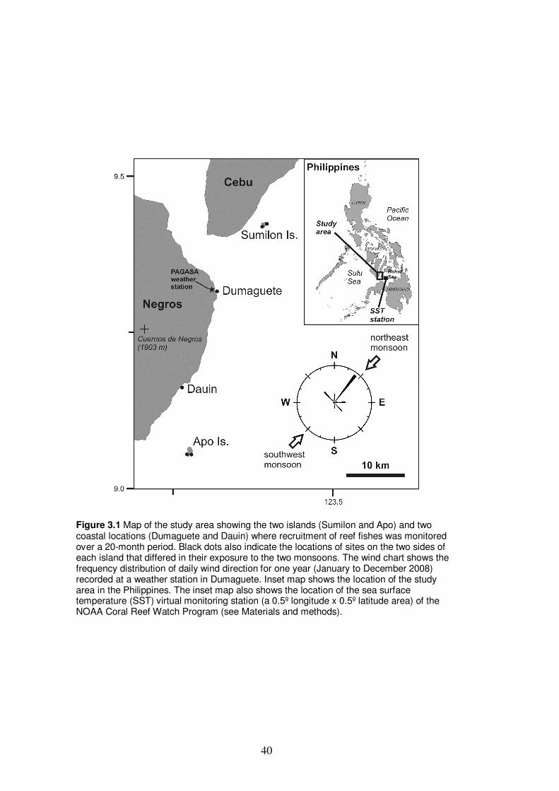
40
Figure 3.1 Map of the study area showing the two islands (Sumilon and Apo) and two coastal locations (Dumaguete and Dauin) where recruitment of reef fishes was monitored over a 20-month period. Black dots also indicate the locations of sites on the two sides of each island that differed in their exposure to the two monsoons. The wind chart shows the frequency distribution of daily wind direction for one year (January to December 2008) recorded at a weather station in Dumaguete. Inset map shows the location of the study area in the Philippines. The inset map also shows the location of the sea surface temperature (SST) virtual monitoring station (a 0.5º longitude x 0.5º latitude area) of the NOAA Coral Reef Watch Program (see Materials and methods).

41
(northeast monsoon) predominate, while from July to September, strong winds blow
from the southwest (southwest monsoon). However, much of the study area is sheltered
from the southwest monsoon due to tall mountains in south-eastern Negros (e.g.,
Cuernos de Negros, elevation: 1,903 m; Figure 3.1). Winds during inter-monsoonal
months (April to June and October) are lighter and more variable in direction. Sea
surface temperature fluctuates by about 3 °C annually (about 27-30 °C) (NOAA Coral
Reef Watch Program, http://coralreefwatch.noaa.gov/satellite/index.html) (Figure 3.2a).
Temperatures are lowest from January to March during the northern hemisphere winter.
During this period, the northeast monsoon brings cool winds from mainland Asia.
Temperatures are highest from June/July to November, during and towards the end of
the southwest monsoon. The wet and dry seasons that are typical of many regions of the
Philippines are not very pronounced in this area, but from November to April rainfall is
usually lower compared to the rest of the year [Type III climate based on classification
by the Philippine Atmospheric, Geophysical and Astronomical Services Administration
(PAGASA) (http://kidlat.pagasa.dost.gov.ph/cab/cab.htm)]. The area may also be
affected by several typhoons annually, but it is situated away from the main path of
typhoons (up to 20 typhoons may affect the Philippines throughout the year).
3.2.2 Study sites
Two small islands and two coastal locations 15-40 km apart were surveyed in
order to gain insights into recruitment patterns within the ~300 km2 study area (Figure
3.1). The two islands were Sumilon (0.2 km2) and Apo (0.7 km
2). They are about 40 km
from each other and about 2 and 7 km away, respectively, from their nearest
neighbouring large island (Negros and Cebu, respectively). Coral reefs surround much
of Sumilon and Apo to a depth of more than 50 m. Reefs are steeper and more
developed along the southern half of the two islands. The two coastal locations were
situated along the south-eastern coast of Negros in Dauin municipality and Dumaguete
City. Dauin and Dumaguete are about 20 km apart. The reefs in both coastal locations
are found less than 300 m from shore between depths of < 1 to 30 m and are patchily
distributed, separated by sand or seagrass.
3.2.3 Visual census of recruits
Samples of monthly recruit abundance of coral reef fish were taken by an
experienced observer (R.A.A.) by counting all non-cryptic recruits along 50 m long x 2

42
m wide belt transects laid parallel to the shoreline following a depth contour. The
sampling strategy aimed to include as many species and reef habitat types as practically
possible. Sampling took place at 11 sites that were unequally distributed among the four
locations, two depths (reef slope and reef flat) and two wind exposures (northeast and
southwest). North-eastern (NE) and south-western (SW) Sumilon, and south-eastern
(SE) and south-western (SW) Apo were sampled. At each of these sides of the two
islands, two depths (3-4 m, 10-12 m) were sampled, each with three replicate transects.
Hard coral cover in the deeper sites (reef slope) of the two islands ranged from 35-70%
except on NE Sumilon where sand, dead coral and rock dominated benthic cover. Soft
corals and/or coral rubble dominated benthic cover in the shallower (reef flat) sites. All
transects in SW Sumilon and SE Apo were situated inside a no-take marine reserve. In
Dauin, surveys were done on coral patches (50-120 m long x 20-80 m wide) found
within a stretch of coast about 1 km long. Only two depths were sampled (3-4 m, 8-12
m), each with five replicate transects. Hard coral cover on those coral patches ranged
from 30-60%. Almost all transects in Dauin were situated inside two no-take marine
reserves. In Dumaguete, the seaward edge of a shallow coral patch (about 200 m long x
100 m wide) was surveyed. Only one depth (3-4 m) was sampled with three replicate
transects. Hard coral cover on this coral patch ranged from 30-35%.
Surveys of recruits were conducted for 19 separate months over a 20-month
period (late February 2008 to early September 2009). The only month that was not
sampled was February 2009 due to inclement weather. Unfavourable weather also
prevented surveys at certain sites during some months: February 2008 (Dumaguete
site); January 2009 (Sumilon and Apo sites); July 2009 (SW Sumilon at 3-4 m); August
2009 (SW Apo sites); and September 2009 (Dauin at 3-4 m). Moreover, replicate
samples were incomplete in Dauin during two months: August 2009 (only 3 transects at
8-12 and 3-4 m) and September 2009 (only 3 transects at 8-12 m). Due to logistical
constraints, random sampling among sites could not be performed but the order in
which islands and coastal locations were surveyed during each month was not fixed.
Within each site, transects had a random starting point wherever practical but the same
general area was sampled almost every month. Sites were located every month with the
aid of fixed natural (rocks, big coral bommies, etc.) and man-made (mooring buoys)
markers at the surface or underwater.
Recruits of a particular month are fish that settled during, and survived to the
end of, a lunar cycle. Past studies and reviews indicated that larval settlement on reefs

43
tends to be higher around the new moon and lower around the full moon (Victor 1986;
Doherty 1991; Wilson 2001). This lunar periodicity of larval settlement was confirmed
in a pilot study at Dauin where the abundance of new recruits settling on 15
individually-marked branching coral colonies were monitored every 2-3 days over 2
lunar cycles (Appendix 3.1). Surveys of recruits were therefore performed around the
full moon (2 days before to 7 days after) in order to capture the peak settlement periods
within each lunar cycle. All sites were sampled within 3-4 days except when field work
was delayed for 2-3 days because of inclement weather. The time interval between
consecutive monthly surveys at each site was about 4-5 weeks (26-35 days; mode = 28
days or 4 weeks). Consistent timing of monthly surveys was used to help reduce
variability in the data caused by mortality of early recruits (due to predation).
In order to avoid counting older fish that did not settle within the previous 4-5
weeks, only those fish that were below an arbitrary threshold size were counted. For
many species the threshold size was set at < 20 mm total length (TL), e.g., damselfishes
(Pomacentridae), wrasses (Labridae), parrotfishes (Scaridae), etc. For species that had
larger recruits, e.g., butterflyfishes (Chaetodontidae) and surgeonfishes (Acanthuridae),
threshold sizes were set at < 30-40 mm TL, respectively. These size limits allowed for
several mm of growth after settlement. Estimates of threshold sizes were guided by
family-level information on sizes of late stage pre-settlement larvae and newly settled
recruits (e.g., Leis and Rennis 1983; Leis and Trnski 1989; Victor 1991; Paddack and
Sponaugle 2008). Data on sizes of newly settled recruits from the pilot study
supplemented the basis for these threshold sizes. Threshold size was set at < 20 mm TL
for species that had no information available on sizes at the recruit stage. In order to
maintain the accuracy of size estimates, the observer always used a ruler attached to the
top of his recording slate as a guide. Recruits that were too small to identify to the
species level were identified to the genus or family level (e.g., Apogonidae).
Benthic composition along each transect was estimated during the first five
months of the survey period. The type of substrate (e.g., hard coral, soft coral,
macroalgae, dead coral, rock, sand, etc.) at every 0.5 m point intercepted by the 50-m
transect was recorded and expressed as a percentage of all points per transect (%
cover). The purpose of the benthic surveys was to provide a baseline description of reef
habitat at each site in order to detect changes in habitat caused by disturbances (e.g.,
coral bleaching, typhoons) that could affect recruit abundance during the study.
However, additional benthic surveys were not conducted after the first five months of
44
the study because the few disturbances (i.e., 3 typhoons) that affected the study area did
not cause major damage to the reef habitat at each site.
3.2.4 Weather data and sea surface conditions
Data on sea surface temperature (SST) for the period covered by the recruitment
surveys were obtained from the NOAA Coral Reef Watch Program
(http://coralreefwatch.noaa.gov/satellite/index.html). The program has a ‘virtual’ SST
monitoring station located in the Bohol Sea close to the study area (Figure 3.1). The
SST monitoring station is a 0.5º longitude x 0.5º latitude area. Data on SST are derived
from nighttime measurements made by the Advanced Very High Resolution
Radiometer (AVHRR) carried on NOAA's Polar Orbiting Environmental Satellites
(POES). The temporal resolution of the data was bi-weekly, giving 7-10 days of SST
measurements for every 4-5 week period covered by the monthly recruitment surveys.
Daily data on wind velocity and rainfall during the recruitment surveys were obtained
from a weather station at Dumaguete airport operated by the PAGASA. This weather
station is located almost at sea level < 1 km from the coast and about 1-30 km away
from the individual recruitment monitoring sites (Figure 3.1). The data on wind showed
that wind speed was highest in January and February during the northeast monsoon and
weakest around July during the southwest monsoon (Figure 3.2b). This wind pattern is
due to the fact that when south-westerly winds predominate, Dumaguete is on the
leeward side of Negros (see wind chart in Figure 3.1). However, the pattern in wind
speed also directly reflects the seasonal change in sea surface conditions within much
of the study area. Wind stress (i.e., drag caused by wind moving over water) causes
seasonality of wave action. Surface waters east of Negros are generally more turbulent
during the northeast monsoon than the southwest monsoon (R. Abesamis, personal
observations over > 2 years). The sheltering effect of Negros during the southwest
monsoon is most noticeable in Dumaguete but can still be felt at Dauin and Sumilon.
Occasionally, however, the two latter sites can be affected by storm surge when the
southwest monsoon is intensified by typhoons. Apo Is., on the other hand, is not
sheltered by Negros during the southwest monsoon. Thus, surface waters around Apo
can be rough during both monsoons. The data on rainfall was probably an accurate
index of rain intensity for the entire study area. Peaks in rainfall during certain months
were caused by the intertropical convergence zone and several typhoons and storms that
affected the area, as opposed to just localized rain in the Dumaguete area (Figure 3.2b).

45
Heaviest rainfall was recorded in early February 2009, when a storm brought more than
250 mm of rain in just one day.
3.2.5 Data analyses
The temporal pattern of ‘collective recruitment’ (i.e., recruits of all species
combined) was described by averaging monthly total recruit density and species
richness across all 11 sites. Significant differences among monthly average values (19
months) were then determined using one-way ANOVA. Planned contrasts were made
after each ANOVA to determine inter-annual and seasonal differences. For inter-annual
comparisons, data from March to September in 2008 were contrasted with data from the
same months in 2009. For comparisons between seasons, data from northeast monsoon
(November to March), southwest monsoon (July to September) and inter-monsoonal
months (April, May, June and October) were contrasted with each other. The overall
temporal pattern of recruitment of two common families, the damselfishes and the
wrasses, were compared. Special interest was given to these two families because they
dominated recruit species composition and comprised 80% of cumulative recruit
abundance. Monthly recruit densities of the damselfishes and wrasses were summarised
and analysed following the same approach as that for total recruit density.
Potential effects of SST, wind speed (as a proxy for wind stress) and rainfall on
the temporal pattern of collective recruitment were tested using multiple regression
analyses. Average recruit density and species richness values were computed for each
location (Sumilon, Apo, Dauin and Dumaguete) for every month surveyed, giving a
sample size of n = 73 for each regression. Monthly values for each environmental
variable were computed by averaging (for SST and wind speed) or summing (for
rainfall) bi-weekly or daily values within each 4-5 week period that corresponded to
each monthly recruitment survey. The potential effects of SST, wind stress and rainfall
on the temporal pattern of recruitment of the damselfishes and wrasses were also tested
following the same procedures.
Most variables were transformed in order to conform to the assumptions of
parametric statistical procedures [log (x + 1) for total recruit density, damselfish
density, wind speed, rainfall; (x)1/2
for species richness; (x + 0.001)0.25
for wrasse
density]. All statistical analyses were performed in Statistica (ver. 8).
Species-level analysis of temporal patterns of recruitment was limited to the
most abundant species, i.e., species that had a cumulative abundance of ≥ 50 recruits

46
recorded from all sites. Only the data from sites where each species was most abundant
were used in this analysis. The duration of the recruitment period of each species was
estimated by counting the number of months when recruitment was considered
significant. To determine which months had significant recruitment, two arbitrary
thresholds of abundance were applied. The first threshold was set at ≥ 1 % of the
adjusted total abundance in one year. This was adapted from Srinivasan and Jones
(2006) and was used in the present study in order to directly compare results between
the central Philippines and Kimbe Bay, Papua New Guinea. The second threshold was
set at ≥ 5 % of the adjusted total abundance in one year to provide more conservative
estimates of duration of the recruitment period. To compute the adjusted total
abundance of a species in one year, average abundance values for each month that was
surveyed for two years (March-September) were initially computed then added to the
raw abundance values of other months. The abundance value of each month was then
expressed as a percentage of the adjusted total abundance in one year.
3.3 Results
A total of 40,913 new recruits of 120 species of reef fish from 16 families were
recorded during the surveys. Species composition was dominated by the damselfishes
(43 species) and wrasses (35 species). Damselfishes comprised 73% of total recruit
abundance, wrasses just 7%. The five most abundant species were four damselfish
species (Pomacentrus moluccensis, Chromis ternatensis, Chromis viridis, and Chromis
retrofasciata) and one species of anthias (Pseudanthias tuka, Serranidae, subfamily
Anthiinae). Together, the recruits of these five species accounted for 54% of the total
number of recruits recorded.
New recruits were observed during all months sampled, but a distinct temporal
pattern was present. Peaks in total recruit density were recorded during the southwest
monsoon and the second inter-monsoonal period of the year, in June-July, July-August
and September-October 2008 and June-July 2009 (Figure 3.2c). Total density during
peak months averaged between 100-140 recruits 100 m-2
. During other months, density
was typically less than 30-50% of peak levels. Lowest levels of recruit density were
observed during the northeast monsoon, in February and March 2008 and December-
January and March-April 2009, averaging between 5-15 recruits 100 m-2
(Figure 3.2c).
This temporal pattern was also evident in the density of recruits of damselfishes and

47
Figure 3.2 Temporal patterns of sea surface temperature, wind speed and rainfall (a, b) versus temporal patterns of recruit density (total, damselfishes, wrasses) and species richness averaged for all sites (c-f). Monsoons indicated by different shades of grey along x-axis. NE = northeast monsoon; SW = monsoon; INT = inter-monsoon. Position of plotted data between calendar months reflects change in timing of lunar months relative to calendar months. Error bars are ± SE. ND = no data.

48
wrasses, notwithstanding a 10-fold difference in abundance of recruits between the two
families (Figure 3.2d-e). However, recruit density of wrasses also peaked in July-
August 2009. The temporal pattern in species richness mirrored the temporal patterns in
density (Figure 3.2f). On average, 10-12 species per 100 m-2
were recruiting during
months of highest recruit densities. In contrast, only 2-7 species per 100 m-2
on average
were recruiting during other months.
Significant differences in monthly levels of recruit densities (total, damselfish and
wrasse) and species richness were detected among the 19 months that were sampled
(Table 3.1). Total recruit density was significantly greater (by 64%) in 2008 than in
2009 (March to September). Similarly, damselfish recruit density was significantly
higher (by 47%) in 2008 than in 2009. However, no significant inter-annual variation
was detected for species richness of recruits and density of wrasse recruits. Significant
variation in recruit densities and species richness was detected between all seasons that
were compared (Table 3.1). Average recruit densities and species richness were always
lowest during the northeast monsoon (November to March), highest during the
southwest monsoon (July to September) and were at intermediate levels during the
inter-monsoonal months (Table 3.1).
Peaks in recruit densities and species richness were recorded during or around
the southwest monsoon, when SST values were highest and wind speed values lowest
(Figure 3.2a-f). Conversely, lowest densities and species richness occurred during the
northeast monsoon, when SST values were lowest and wind speed values highest.
Regression models indicated significant effects of SST and wind speed on monthly
average recruit densities and species richness (Table 3.2). SST always had a positive
effect, and wind speed always had a negative effect, on recruitment. The models,
however, did not suggest any significant effect of rainfall on recruit densities or species
richness (Table 3.2, Figure 3.2b-f).
There was a good degree of spatial coherence in the general pattern of monthly
collective recruitment (Figure 3.3). The peaks in recruit density during the southwest
monsoon and the second inter-monsoonal period, and the troughs during the northeast
monsoon were detected across most sites (Figure 3.3a). However, the peak in
recruitment in June-July 2009 was obvious at only a few sites, and there were peaks
during March-April in 2008 and 2009 that were recorded only in some sites.
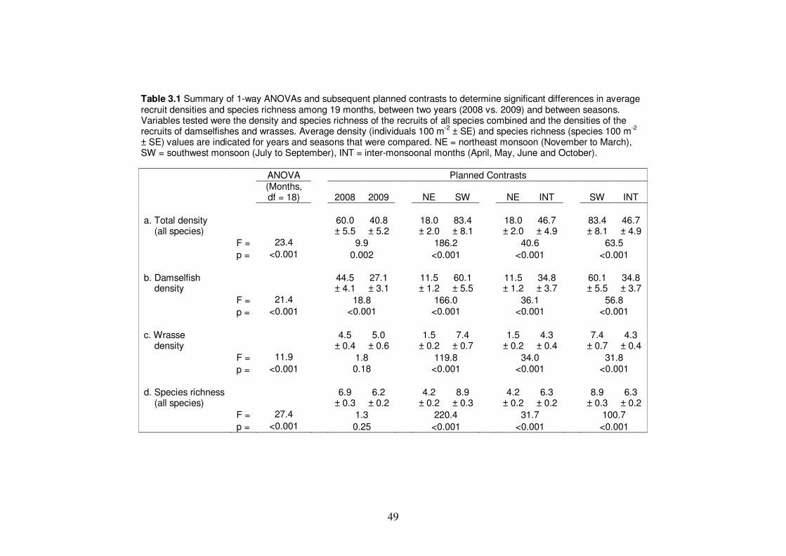
49
ANOVA Planned Contrasts
(Months, df = 18) 2008 2009 NE SW NE INT SW INT
a. Total density (all species)
60.0 ± 5.5
40.8 ± 5.2
18.0 ± 2.0
83.4 ± 8.1
18.0 ± 2.0
46.7 ± 4.9
83.4 ± 8.1
46.7 ± 4.9
F = 23.4 9.9 186.2 40.6 63.5
p = <0.001 0.002 <0.001 <0.001 <0.001
b. Damselfish density
44.5 ± 4.1
27.1 ± 3.1
11.5 ± 1.2
60.1 ± 5.5
11.5 ± 1.2
34.8 ± 3.7
60.1 ± 5.5
34.8 ± 3.7
F = 21.4 18.8 166.0 36.1 56.8
p = <0.001 <0.001 <0.001 <0.001 <0.001
c. Wrasse density
4.5 ± 0.4
5.0 ± 0.6
1.5 ± 0.2
7.4 ± 0.7
1.5 ± 0.2
4.3 ± 0.4
7.4 ± 0.7
4.3 ± 0.4
F = 11.9 1.8 119.8 34.0 31.8
p = <0.001 0.18 <0.001 <0.001 <0.001
d. Species richness (all species)
6.9 ± 0.3
6.2 ± 0.2
4.2 ± 0.2
8.9 ± 0.3
4.2 ± 0.2
6.3 ± 0.2
8.9 ± 0.3
6.3 ± 0.2
F = 27.4 1.3 220.4 31.7 100.7
p = <0.001 0.25 <0.001 <0.001 <0.001
Table 3.1 Summary of 1-way ANOVAs and subsequent planned contrasts to determine significant differences in average recruit densities and species richness among 19 months, between two years (2008 vs. 2009) and between seasons. Variables tested were the density and species richness of the recruits of all species combined and the densities of the recruits of damselfishes and wrasses. Average density (individuals 100 m
-2 ± SE) and species richness (species 100 m
-2
± SE) values are indicated for years and seasons that were compared. NE = northeast monsoon (November to March), SW = southwest monsoon (July to September), INT = inter-monsoonal months (April, May, June and October).

50
Model SST Wind speed Rainfall
R2
adj F p Rp t p Rp t p Rp t p
a. TD 0.45 20.71 <0.001 0.35 3.10 0.003 -0.41 -3.71 <0.001 -0.12 -1.03 0.30
b. DD 0.43 19.30 <0.001 0.33 2.90 0.005 -0.40 -3.64 0.001 -0.08 -0.67 0.50
c. WD 0.36 14.56 <0.001 0.37 3.34 0.001 -0.27 -2.36 0.02 -0.14 -1.15 0.25
d. SR 0.52 27.02 <0.001 0.42 3.84 <0.001 -0.43 -3.96 <0.001 -0.17 -1.44 0.16
A total of 37 species, representing 7 families, had a cumulative abundance of ≥
50 recruits recorded from all sites during the study (Appendix 3.2). The species
composition of this subset of species was still dominated by the damselfishes (23
species), followed by the wrasses (6 species). Most of these 37 species had protracted
annual recruitment periods. Depending on the threshold value that was used, the
majority of species (23-24 species in 5-6 families) had 5-7 or 9-11 months of significant
recruitment (Figure 3.4a, b). The shortest recruitment periods were found only in a few
species of damselfish (e.g., Chromis amboinensis, Dascyllus trimaculatus,
Neopomacentrus anabatoides, N. azysron, Pomacentrus smithii) and the cardinalfishes
(Apogonidae) (Figure 3.4a, b). There was considerable variation in the timing of peaks
among species but most peaks occurred during the southwest monsoon and inter-
monsoonal months, mainly in July and October (Figure 3.5). Most of the major peaks
that contributed substantially to the cumulative annual abundance of each species were
also recorded in July or October. Within the damselfishes, the timing of major peaks of
Neoglyphidodon, Neopomacentrus and most Pomacentrus spp. differed from that of
Chromis, Chrysiptera, and Dascyllus spp. in that the major recruitment peaks in the
former group occurred earlier than in the latter group. At the family level, the timing of
recruitment peaks of the damselfishes, wrasses, parrotfishes, anthiases and
cardinalfishes were more similar to each other compared to the butterflyfishes and
Table 3.2 Summary of regression models to assess the potential effects of environmental variables on temporal patterns of recruitment. Dependent variables were the monthly total density (TD) and species richness (SR) of the recruits of all species combined and the monthly densities of recruits of the two families (damselfishes and wrasses – DD and WD, respectively) that dominated recruit species composition and overall abundance. Monthly density and species richness values were averaged for each location (Sumilon, Apo, Dauin and Dumaguete), resulting in n = 73 for each regression. Independent variables were monthly average sea surface temperature (SST), average wind speed (as the proxy for wind stress) and total rainfall. R
2adj = adjusted R
2 value of the regression model, Rp = partial correlation coefficient of
independent variable.

51
Figure 3.3 Temporal patterns of (a) total recruit density and (b) species richness at all sites. A = northeast Sumilon, 3-4 m; B = northeast Sumilon, 10-12 m; C = southwest Sumilon, 3-4 m; D = southwest Sumilon, 10-12 m; E = southeastern Apo, 3-4 m; F = southeastern Apo, 10-12 m; G = southwest Apo, 3-4 m; H = southwest Apo, 10-12 m; I = Dauin, 3-4 m; J = Dauin, 8-12 m; K = Dumaguete, 3-4 m. Monsoons indicated by different shades of grey along x-axis. NE = northeast monsoon; SW = monsoon; INT = inter-monsoon. ND = no data.

52
Figure 3.4 Durations of the recruitment period (months) of the 37 most abundant species (grouped into 7 families in this figure) estimated using two thresholds of recruit abundance per month: ≥ 1% (a) and ≥ 5% (b) of adjusted total abundance in one year (see Materials and methods).
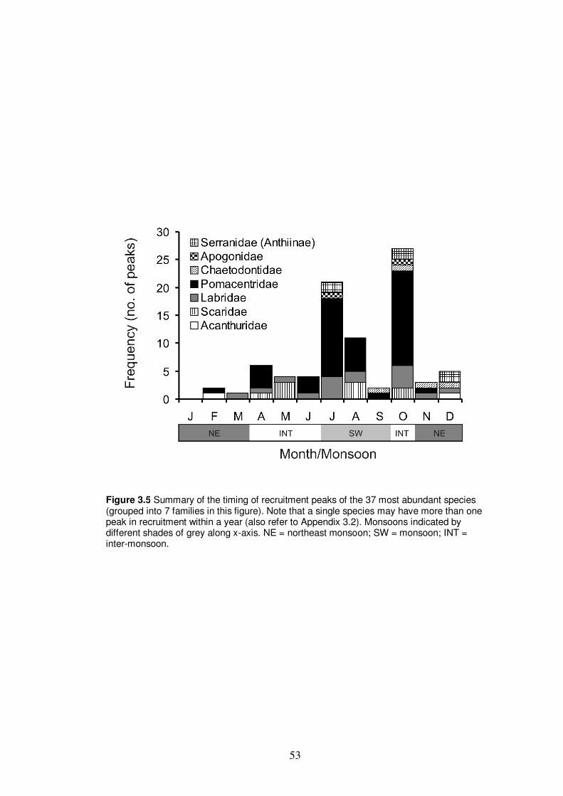
53
Figure 3.5 Summary of the timing of recruitment peaks of the 37 most abundant species (grouped into 7 families in this figure). Note that a single species may have more than one peak in recruitment within a year (also refer to Appendix 3.2). Monsoons indicated by different shades of grey along x-axis. NE = northeast monsoon; SW = monsoon; INT = inter-monsoon.
54
surgeonfishes (Appendix 3.2). Recruitment peaks of the two latter families, which were
represented by one species each (Chaetodon baronessa and Ctenochaetus binotatus,
respectively), only occurred in the earlier or later part of the year, almost all during the
northeast monsoon (Figure 3.5).
3.4 Discussion
This study is one of the few to describe patterns of recruitment (settlement) of
coral reef fishes in a location within the Indo-Pacific region where reversing monsoon
winds strongly influence environmental conditions. Previous studies have suggested
that the monsoons play a role in determining the annual pattern of recruitment of fishes,
particularly in the Philippines (Pauly and Navaluna 1983; McManus et al. 1992; Arceo
2004; Cabaitan et al. 2008). However, the present study is the first in the Philippines
that related observed patterns of recruitment of fishes directly to environmental data.
New recruits were observed throughout the year and the majority of species that
were examined exhibited protracted recruitment seasons. These results confirm the
expectation of extended annual breeding of reef fishes at lower latitudes (Robertson
1990; Doherty 1991; Srinivasan and Jones 2006; see also Chapter 2). Of greater
significance, the annual pattern of collective recruitment was predictable. Annual
variability in SST and wind strength can largely account for the pattern. There was a
good degree of similarity in the pattern of recruitment among sites considering the
distance separating them (up to 40 km), differences in exposure to prevailing monsoon
winds, habitat and depth, and large differences (up to 20-fold) in maximum average
recruit densities between some sites. This indicates that the effects of SST and wind
were working at a broad spatial scale, most likely during the pelagic larval phase.
Rainfall, on the other hand, did not have a significant effect on the patterns of
recruitment.
Results strongly suggested that the best ‘window’ for survival and settlement of
larvae of the most common reef fish species (mostly damselfishes and wrasses) is
during a 4-6 month period within the year when water temperatures are warmest and
when winds are weakest locally, i.e., during the southwest monsoon and inter-
monsoonal periods. Small increases in water temperature can enhance growth rates of
larval reef fishes (McCormick and Molony 1995; Wilson and Meekan 2002; Meekan et
al. 2003; Bergenius et al. 2005; Sponaugle et al. 2006). Faster growth, in turn, can

55
result in higher survivorship because fewer predators would be capable of preying on
larger larvae and the time spent in the pelagic environment is shortened (Houde 1987;
Anderson 1988). For instance, Wilson and Meekan (2002) showed that in San Blas in
the Caribbean Panama, where water temperature varies by only about 3 ºC, temperature
is positively correlated with larval growth and magnitude of settlement of the
damselfish Stegastes partitus (also see Bergenius et al. 2002). On the other hand, wind
can result in two physical processes that have potential consequences for the pelagic
larval phase. Firstly, wind stress can generate waves and turbulent mixing of surface
waters which may be detrimental to survival. Some field studies have indicated that
mortality rates in fish larvae are highest during windy conditions, probably because
turbulence disrupts concentrated patches of food that are critical to the survival of first-
feeding larvae (Peterman and Bradford 1987; Bailey and Macklin 1994). At very small
spatial scales, mild turbulent mixing could increase the encounter rates between larval
fish and their prey (MacKenzie and Kiorboe 1995; Utne-Palm and Stiansen 2002; Utne-
Palm 2004). However, this may increase feeding success and result in faster growth
rates in larval fish (Gallego et al. 1996), thus potentially enhancing settlement.
Secondly, prevailing winds can influence dispersal of larvae over larger spatial
scales (10’s to 100’s of kilometres) (Sponaugle and Cowen 1996). There is some
suggestion that the effect of the monsoon winds on surface current patterns in the Bohol
Sea can partly explain the observed annual pattern of recruitment. In the Bohol Sea,
there is a dominant westward flow produced by water entering from the Pacific Ocean
and exiting to the Sulu Sea through the Negros-Mindanao strait (Wyrtki 1961). In the
study area, this dominant current is manifested as a strong south-westward flow
(Chapters 2, 4). Data from a sea surface circulation model [1/32º global Navy Layered
Ocean Model (NLOM), see Shriver et al. 2007] indicate that this current is enhanced by
the northeast monsoon, increasing the potential for flushing of eggs and early-stage
larvae out of the study area (Figure 4.2). During the southwest monsoon and inter-
monsoonal periods, the current weakens, potentially enhancing retention of larvae. If a
good proportion of the recruits that settle on reefs that were studied are produced in the
same general locality (as opposed to more distant reefs), then monsoon-induced
seasonal variation in the strength of local currents will have a significant influence on
the annual pattern of recruitment. In such a case, the potential effect of wind on local
settlement is negative only when it enhances the dispersal of larvae away from nearby
source reefs.

56
A comparison of the findings of the present study with similar studies from
other locations close to the equator indicates that among environmental variables, wind
has the most consistent effect on settlement patterns of reef fishes, particularly in
damselfishes and wrasses. For instance, the annual patterns of recruitment of
damselfishes and wrasses that were described here are similar to the recruitment
patterns of several damselfish species and one species of wrasse (Thalassoma
bifasciatum) in San Blas, Caribbean Panama (~9.5 ºN) (Robertson 1990; Robertson et
al. 1999). Recruitment of these fishes in San Blas is lower during the dry season
(December to April) when northerly tradewinds produce heavy wave action. Species-
specific peaks in recruitment occur throughout the wet season (May to November)
when winds are lighter. Other studies at San Blas have recorded similar seasonality of
larval supply of damselfish and T. bifasciatum (Victor 1986; Wilson 2001). In northern
Philippines, McManus et al. (1992) monitored monthly fish recruitment on the reef
slope of the Bolinao reef system (~16.5 ºN) for four consecutive years. They found one
annual peak in total recruitment in that area every year. The recruitment peak occurred
between April and July, coinciding with the first inter-monsoonal period when winds
are weakest in that area. Note that unlike the area that was surveyed in the present
study, the Bolinao area is exposed to the north-east and south-west monsoon winds.
Wind also appears to strongly influence the patterns of reef fish recruitment on lower
latitude reefs in the southern hemisphere. In Kimbe Bay, Papua New Guinea (~5.5º S),
recruitment of many species of wrasses (but not damselfishes) is lower between July
and August when monsoon winds are strongest (Srinivasan and Jones 2006).
Some general effects of wind, water temperature, and rainfall emerge from the
few studies of reef fish recruitment carried out at low latitude sites to date. The annual
trend in wind strength in relation to temperature is somewhat similar between the
Philippine and Caribbean sites studied (Lemberget et al. 2009; this study). It is likely
that in other lower latitude sites with similar environmental conditions, wind and
temperature interact to influence recruitment patterns of many species. However,
further insights about temperature are precluded by the absence of an evaluation of its
effect on fish recruitment patterns at other locations such as Kimbe Bay (the annual
water temperature range there is < 2º C) (Srinivasan and Jones 2006). Studies to date
suggest that rainfall is influential only in areas that have an extremely pronounced wet
season. For example, in Kimbe Bay, strong rainfall may persist for many weeks, and
reach more than 600 mm month-1
during the wet season (Srinivasan and Jones 2006).
57
Heavy rainfall at that site seemed to negatively affect the recruitment of damselfishes
(Srinivasan and Jones 2006). In contrast, rainfall at the Philippine and Caribbean sites is
considerably less during the wet season than in Kimbe Bay and had little effect on the
recruitment of damselfishes and wrasses (Robertson 1990; Robertson et al. 1999; this
study).
It is tempting to extrapolate the seemingly predictable effects of water
temperature, wind and rainfall to the recruitment patterns of reef fishes in all equatorial
regions. However, such predictable effects for all equatorial regions are unlikely.
Recruitment patterns of one butterflyfish and one surgeonfish in this study were
opposite to the dominant pattern, i.e. settlement in these species was more favourable
during the cooler and windier months. Other studies conducted at lower latitude reefs,
including those that investigated the effects of environmental variables on larval
development and settlement success in detail, highlight species-specific responses and
contrasting patterns even among closely-related species (Sponaugle and Cowen 1994,
1997; Robertson and Kauffman 1998; Bergenius et al. 2005; Lemberget et al. 2009).
There are few studies on the seasonal patterns of spawning and recruitment of
reef fishes in the Philippines (Chapter 2). This limits an assessment of the degree to
which spawning activity may affect patterns of recruitment in reef fishes within the
Philippines. In the preceding study (Chapter 2), data on the annual spawning pattern of
one population of P. moluccensis at one site (Dumaguete) where recruitment of this
species was also monitored suggest minimal spawning activity during the northeast
monsoon (Figure 2.5). Results of the present study indicate that this pattern of
spawning is consistent with the annual pattern of recruitment of P. moluccensis at that
site and at most sites where P. moluccensis recruits were abundant (Dauin and Apo Is.)
(Figure 3.1). If the patterns of spawning and recruitment in P. moluccensis are strongly
coupled, then the same pattern of spawning in this species should be evident at other
sites. However, the findings of Chapter 2 imply that the annual pattern of spawning in
P. moluccensis will vary among local populations depending upon their degree of
exposure to the two monsoon winds. Furthermore, the present study indicates that
patterns in recruitment are influenced more by environmental factors that are working
at a broad spatial scale during the pelagic larval phase as opposed to environmental
conditions at more local spatial scales. On the other hand, strong coupling between
patterns of spawning and recruitment is exhibited by rabbitfishes in the Bolinao reef
system. For instance, spawning migrations of the rabbitfish Siganus fuscescens occur

58
twice a year (March-May and August-September), resulting in two major annual
recruitment peaks (Aragones 1987; McManus et al. 1992). The timing of spawning and
recruitment in this species is remarkable because it appears to perfectly match the two
inter-monsoonal periods within the year, when winds are weakest.
This study is an initial step in understanding the dynamics of recruitment of
fishes on Indo-Pacific coral reefs situated in monsoonal environments. Similar studies
in other equatorial locations that differ in the character of the monsoons and the degree
of exposure to monsoonal conditions are needed. More attention should also be given to
resolving the patterns of spawning at the same locations (Chapter 2) to test hypotheses
about the degree of coupling between timing of reproduction and larval survival. A
reliable understanding of the role of the monsoons, temperature and rainfall in shaping
the seasonality of spawning and recruitment may prove useful in determining year-to-
year recruitment strength, something that remains difficult to predict for fish
populations at lower latitude reefs because of extended annual breeding periods. Better
knowledge on the spatial and temporal patterns of reef fish reproduction and
recruitment will also be valuable to conservation and fisheries management efforts,
particularly the use of networks of no-take marine reserves that aim to preserve or
enhance larval connectivity among local reef fish populations (Chapters 4 and 5).

59
Chapter 4
Predicting connectivity in a marine reserve network from reef fish
assemblage patterns and larval dispersal models
Abstract. Connectivity through larval dispersal and recruitment may greatly influence
the dynamics and management of marine populations. Two techniques were used
together to determine potential larval connectivity between populations of coral reef
fishes in a 300-km-wide region in the Philippines that included the Bohol Sea and
adjacent bodies of water. A westward current flows through the Bohol Sea. This current
possibly connects more than 100 no-take marine reserves by larval dispersal. The first
technique investigated connectivity by analysing data on the presence/absence of 216
species of reef fish and habitat variables across 61 sampling sites. Hierarchical
clustering of sites reflecting species assemblage patterns distinguished a major group of
sites in the Bohol Sea (Bray-Curtis species assemblage similarity > 70%) from sites
situated in adjacent bodies of water (i.e., bays, channels and a local sea). The grouping
of sites could be partly explained by a combination of degree of embayment, % cover
of sand and % cover of rubble (Spearman rank correlation, ρw = 0.42). The second
technique predicted patterns of connectivity using an individual-based model that
simulated dispersal of reef fish larvae monthly for 3 consecutive years (2006-2009) in
the Bohol Sea. The results of simulations, using a range of pelagic larval durations (15-
45 days), were consistent with hydrodynamic and reef fish species assemblage patterns.
The sites in the larval dispersal model that showed strongest connectivity corresponded
to the majority of sites that comprised the Bohol Sea group of sites based on fish
assemblage analysis. Most sites in the model that exhibited weak connectivity were
groups of sites which had fish species assemblages that were most dissimilar to those in
the Bohol Sea group of sites. The coincident findings from the two independent
techniques indicated a strong influence of the local hydrodynamic regime on potential
patterns of population connectivity at a broad scale. However, resolution of
connectivity was made difficult by the effect of local habitat on the structure of the reef
fish assemblage.
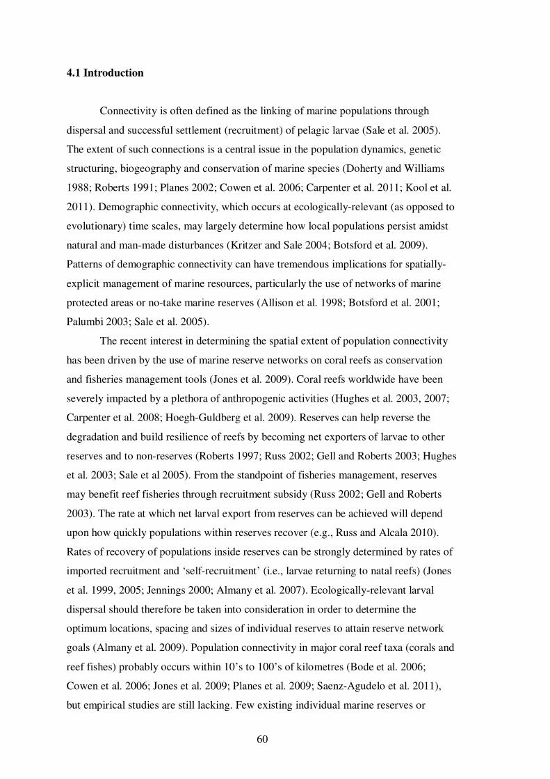
60
4.1 Introduction
Connectivity is often defined as the linking of marine populations through
dispersal and successful settlement (recruitment) of pelagic larvae (Sale et al. 2005).
The extent of such connections is a central issue in the population dynamics, genetic
structuring, biogeography and conservation of marine species (Doherty and Williams
1988; Roberts 1991; Planes 2002; Cowen et al. 2006; Carpenter et al. 2011; Kool et al.
2011). Demographic connectivity, which occurs at ecologically-relevant (as opposed to
evolutionary) time scales, may largely determine how local populations persist amidst
natural and man-made disturbances (Kritzer and Sale 2004; Botsford et al. 2009).
Patterns of demographic connectivity can have tremendous implications for spatially-
explicit management of marine resources, particularly the use of networks of marine
protected areas or no-take marine reserves (Allison et al. 1998; Botsford et al. 2001;
Palumbi 2003; Sale et al. 2005).
The recent interest in determining the spatial extent of population connectivity
has been driven by the use of marine reserve networks on coral reefs as conservation
and fisheries management tools (Jones et al. 2009). Coral reefs worldwide have been
severely impacted by a plethora of anthropogenic activities (Hughes et al. 2003, 2007;
Carpenter et al. 2008; Hoegh-Guldberg et al. 2009). Reserves can help reverse the
degradation and build resilience of reefs by becoming net exporters of larvae to other
reserves and to non-reserves (Roberts 1997; Russ 2002; Gell and Roberts 2003; Hughes
et al. 2003; Sale et al 2005). From the standpoint of fisheries management, reserves
may benefit reef fisheries through recruitment subsidy (Russ 2002; Gell and Roberts
2003). The rate at which net larval export from reserves can be achieved will depend
upon how quickly populations within reserves recover (e.g., Russ and Alcala 2010).
Rates of recovery of populations inside reserves can be strongly determined by rates of
imported recruitment and ‘self-recruitment’ (i.e., larvae returning to natal reefs) (Jones
et al. 1999, 2005; Jennings 2000; Almany et al. 2007). Ecologically-relevant larval
dispersal should therefore be taken into consideration in order to determine the
optimum locations, spacing and sizes of individual reserves to attain reserve network
goals (Almany et al. 2009). Population connectivity in major coral reef taxa (corals and
reef fishes) probably occurs within 10’s to 100’s of kilometres (Bode et al. 2006;
Cowen et al. 2006; Jones et al. 2009; Planes et al. 2009; Saenz-Agudelo et al. 2011),
but empirical studies are still lacking. Few existing individual marine reserves or

61
networks of marine reserves on coral reefs have incorporated quantitative estimates of
larval dispersal and recruitment to their designs (Almany et al. 2009; McCook et al.
2009) or have convincingly demonstrated larval connections among reserves or
between reserves and fished areas (e.g., Gell and Roberts 2003; Pelc et al. 2009, 2010;
Planes et al. 2009; Christie et al. 2010).
Empirical studies of larval dispersal are hindered by many challenges inherent
to larval biology. Most coral reef fishes, for instance, have minute larvae (typically < 20
mm in length before settlement) that undergo ontogenetic development away from reefs
lasting from a few to several weeks, depending on the species (Leis and Rennis 1983;
Victor 1991). Larval distributions in the marine environment are difficult to predict due
to advection by currents and high rates of larval mortality (Leis 1991; Cowen et al.
2000). Also, many late-stage larval reef fishes are capable of sustained directed
swimming that can modify transport trajectories indicated by hydrodynamic patterns
(Stobutzki and Bellwood 1997; Wolanski et al. 1997; Cowen 2002; Leis and
McCormick 2002; Paris and Cowen 2004; Leis 2006). Some of these tremendous
challenges have been addressed by technological advancements in fields such as
oceanography, genetics and chemistry. Various techniques are presently available to
make inferences about connectivity (Jones et al. 1999, 2005; Thorrold et al. 2006;
Almany et al. 2007; Cowen et al. 2007; Hellberg 2007; Werner et al. 2007; Jones et al
2009; Planes et al. 2009; Williamson et al. 2009; Christie et al. 2010; Saenz-Agudelo et
al. 2011). Besides population genetics (particularly parentage analysis) and direct
tagging of larval otoliths using chemical markers (e.g., Jones et al. 1999; 2005; Almany
et al. 2007; Planes et al. 2009) the most applicable technique to measure connectivity at
spatial scales relevant to networks of marine reserves (100’s of kilometres) is
biophysical (larval dispersal) modelling. The current consensus is that connectivity can
be best incorporated into designs of reserve networks using sophisticated biophysical
models that are cross-validated by genetic or otolith chemical tagging techniques that
can relate individual juveniles to their parents (Jones et al. 2009).
Biogeographic studies may also provide clues about reef connectivity at spatial
scales similar to those addressed by biophysical models (Jones et al. 2009). Such
studies are expected to differ from biophysical models particularly in terms of the
temporal scale of larval dispersal. Biophysical models may be limited to predicting
patterns of larval dispersal within decadal time scales (James et al. 2002; Bode et al.
2006; Cowen et al. 2006), while some biogeographic studies (e.g., phylogeography)

62
may detect connectivity that probably occurred hundreds to thousands of years ago, or
much longer (Planes 2002; Rocha et al. 2002; Carpenter et al. 2011). A straightforward
biogeographic approach is to examine larval connectivity indirectly from patterns of
distribution of species. This approach has been used to infer larval dispersal at oceanic
spatial scales (1000’s of km) that presumably occurred over longer time scales
(Thresher and Brothers 1985, 1989). Species distributions have also been used to argue
for the presence or absence of connectivity at more local spatial scales (100’s of km,
e.g., cross-continental-shelf distribution of reef fishes on the Great Barrier Reef and
distributions of reef fish in the Red Sea, see Williams et al. 1986; Roberts 1991;
Roberts et al. 1992). However, the time frame of connectivity that determines these
patterns over shorter distances is almost impossible to know precisely from data on
species distributions alone. An exception to this is the colonisation of the Hawaiian
islands by introduced species of reef fish that occurred over a few decades (Randall
1987). A dearth of studies curtails a critical assessment of the usefulness of species
distributions to infer patterns of population connectivity at scales most relevant to
marine reserve networks.
The utility of species distribution patterns to infer larval connectivity will
depend also upon the extent to which demographic patterns determined by larval supply
are modified by post-recruitment processes. Demographic patterns in reef fishes may be
influenced strongly by a suite of processes acting on the benthic (post-settlement)
juvenile or adult phase (Jones 1991). One process that clearly has a considerable
influence on the patterns of distribution of fishes on coral reefs is habitat selection
(Williams 1991). Abundance and species diversity of reef fishes are usually correlated
with habitat availability and structure (e.g., Carpenter et al. 1981; Roberts and Ormond
1987). Studies of larval connectivity that utilise species distribution patterns must
therefore consider the potential effects of both larval supply and habitat. For two
hypothetical sites in question, the interaction of larval exchange between sites and the
characteristics of reef habitat at each site may result in either similar or dissimilar
species assemblages, for a variety of potential reasons (Table 4.1). The probability,
direction and strength of larval exchange can be predicted and examined using a
biophysical model that includes a range of larval life histories. Habitat and species
assemblage structure at each site, on the other hand, can be measured by field surveys.
From these sets of data, one may infer if larval connectivity is likely to be present or
absent, or if levels of connectivity are strong or weak, between sites (Table 4.1).

63
Connectivity is likely to be significant if larval exchange is probable and strong and the
habitats at the two sites are similar, resulting in similar species assemblages between
sites (Table 4.1, Case 1). However, detecting connectivity becomes uncertain when
larval exchange is probable and strong but the habitats at the two sites are very
different, resulting in species assemblages that are dissimilar between sites (Table 4.1,
Case 2). Connectivity is likely to be absent or weak when larval exchange is predicted
to be improbable or weak and species assemblages are dissimilar between sites,
whether habitats at the two sites are similar or are different (Table 4.1, Cases 3 and 4).
The four preceding cases assume that the predictions of the biophysical model,
measurement of habitat parameters and representation of species assemblage patterns
are all accurate. All four preceding cases also assume that habitat is the most influential
post-recruitment factor structuring assemblages. Failure of any one of these
assumptions may be suspected in four other cases (Table 4.1, Cases 5-8).
Current evidence suggests that patterns of demographic connectivity in coral
reef taxa may be influenced more by local geographic setting than by other factors (e.g.,
Case
Predicted larval
exchange
Measured
habitat
Measured
species
assemblage
Possible conclusions
1 Probable, strong Similar Similar Connectivity likely to be significant
2 Probable, strong Different Dissimilar Connectivity is uncertain
3 Improbable, weak Similar Dissimilar Connectivity likely to be absent or
weak
4 Improbable, weak Different Dissimilar Connectivity likely to be absent or
weak
5 Probable, strong Similar Dissimilar
- Failure to account for the most
influential post-recruitment process
(e.g. disturbances)
6 Probable, strong Different Similar - Failure to measure the most
influential habitat parameter/s
7 Improbable, weak Similar Similar - Failure of biophysical model to
predict connectivity accurately
8 Improbable, weak Different Similar - Failure to measure species
assemblage accurately
Table 4.1 Combinations of predicted larval exchange between, and measured habitat and species assemblage structure within, two theoretical sites. The final column lists possible conclusions about connectivity between the two sites.

64
size of reef habitat or pelagic larval duration) (Jones et al. 2009). Case studies of larval
connectivity within specific networks of marine reserves may therefore be of value to
both reef ecologists and managers. In this study, two techniques were used in
conjunction to determine the extent of potential larval connectivity of reef fish
populations within a 300-km-wide region in the central Philippines that has > 100 ‘no-
take’ marine reserves. The reserves in this archipelagic region were established with
local (community-based) objectives with little consideration of reserve network
planning, but their locations reflect potential connectivity suggested by large-scale
hydrodynamic patterns (Indab and Suarez-Aspilla 2004; Alcala and Russ 2006;
McCook et al. 2009) and relatively short distances (< 5-10 km) separating individual
reserves (Weeks et al. 2010a). The first technique examined patterns of reef fish species
assemblages and associated habitats across multiple sampling sites. A secondary aim of
using this biogeographic approach was to test if species assemblage patterns are useful
in elucidating patterns of larval connectivity at the spatial scale in question. The second
technique used an individual-based larval dispersal model to predict patterns of
connectivity and quantify levels of self-recruitment within, and larval exchange
between, sites. The main expectation of this study was mutual agreement of probable
connectivity, where it exists, by the two independent approaches.
4.2 Materials and methods
4.2.1 The study region
This study was conducted in a region of the central Philippines that included the
Bohol Sea and adjacent bodies of water (Figure 4.1). The Bohol Sea spans about 300
km from east to west and has a mean depth of approximately 1500 m. It is one of the
pathways of water from the Pacific Ocean to the Sulu Sea, connected to the Pacific by
Surigao Strait (~20 km wide) and to the Sulu Sea by Negros-Mindanao Strait (~45 km
wide) (Figure 4.1a). On its northern side, the Bohol Sea is linked to two internal
Philippine seas (Visayan Sea and Camotes Sea) by three channels: Tañon Strait, Cebu-
Bohol channel and Bohol-Leyte channel (Figure 4.1a). At least 16 major and minor
bays are connected to the Bohol Sea. Most of these bays are coastal features of
surrounding major islands: e.g., Sogod and Cabalian bays in Leyte; Cogtong,
Guindulman, Maribojoc bays in Bohol; Gingoog, Butuan, Macajalar, Iligan and
Murcielagos bays in Mindanao) (Figure 4.1b).

65
Figure 4.1 Maps of the study region (Bohol Sea and adjacent bodies of water). The top map (a) shows the names of major islands and adjacent bodies of water that were included in this study. It also shows the locations of numerous ‘no-take’ marine reserves (black circles). The middle map (b) indicates the locations of 61 sites where surveys of reef fishes and benthic habitat were undertaken (black squares). The names of numerous small islands and bays are indicated. The bottom map (c) shows the spatial domain of the biophysical individual-based (larval dispersal) model. It also indicates grid cells that were classified as areas of coral reef (grey squares). Coral reef grid cells that were designated as spawning sites for virtual larvae are marked by white circles. These spawning sites were grouped into 15 nodes (encircled).
66
Figure 4.2 Annual trend in current patterns within the study region represented by three months: January (a), May (b) and August (c). January represents current patterns for 6 consecutive months of the year (November to April), coinciding with the northeast monsoon wind. May and August represent current patterns for inter-monsoonal and southwest monsoon (June to September) periods, respectively. Velocity vectors were averaged from 3 years (June 2006 to May 2009) of data interpolated from NLOM (see Materials and methods). Strongest currents (> 0.10 to 0.80 m sec
-1) are highlighted in
grey. Maximum average velocities estimated for January, May and August were 0.80, 0.60 and 0.47 m sec
-1, respectively.

67
Wyrtki (1961) showed that the net flow of surface water in the Bohol Sea is
westward throughout the year. This surface current pattern is also indicated by in situ
data collected during oceanographic surveys (Cabrera et al. 2011; Lermusiaux et al.
2011). Data from the U.S. Navy Layered Ocean Model (NLOM) (www7320.nrlssc.
navy.mil/global_nlom) indicate that this westward surface flow is usually strongest near
the northern boundary of the sea for 6 consecutive months of the year (November to
April), coinciding with the northeast monsoon (Figure 4.2a). During this period, the
dominant current passes within the vicinity of the southern coasts of four major islands
(Leyte, Bohol, Cebu and Negros), around a fifth island (Siquijor) and in the vicinity of
the north-western tip of Mindanao, before exiting through the Negros-Mindanao Strait
(Figure 4.2a). During inter-monsoonal periods
(e.g., in May), the westward mainstream current weakens slightly and meanders,
forming eddies (Figure 4.2b). During the southwest monsoon (e.g., in August), it
weakens further and may shift its position closer to the southern boundary of the Bohol
Sea (Figure 4.2c).
The westward mainstream current has been hypothesised to be a dominant
driver of the patterns of connectivity between coral reef populations in the Bohol Sea
(Ablan 2005, 2006; Alcala and Russ 2006; McCook et al. 2009). This study focused on
investigating potential larval connectivity among fish populations on coral reefs
situated mainly along the northern boundary of the Bohol Sea due to the persistence of
the westward mainstream current in that area (Figures 4.1 and 4.2). To date, there are
an estimated 112 small (i.e., area < 1 km2 per reserve) community-based no-take marine
reserves located within that area (Alcala et al. 2008; Weeks et al. 2010a) (Figure 4.1a).
The history of establishment and management status of these reserves are described in
detail by Russ and Alcala (1999), White et al. (2002), Indab and Suarez-Aspilla (2004),
Alcala and Russ (2006), Alcala et al. (2008) and Weeks et al. (2010a).
4.2.2 Reef fish and benthic habitat data
The data on reef fishes and benthic habitat for this study were selected from a
large set of data collected during surveys of coral reefs in the central Philippines (Russ
et al. 2005; Stockwell et al. 2009). The objective of most of these surveys was to
investigate spatial variations in the effects of no-take marine reserves on reef fish
communities. Data from 61 sites were used. The sites formed a transect spanning more
than 300 km from east to west mostly across the northern part of the Bohol Sea (Figure
68
4.1b). Thirty-six of the sites were no-take reserves. The rest were areas of reef open to
fishing. The selected sites were situated along the coasts of southern Leyte, Bohol,
Negros, northern and southern Siquijor, and north-western (NW) Mindanao (Figure
4.1b). Seventeen of the sites were located within bodies of water connected to the
Bohol Sea but not directly influenced by the mainstream westward current. These
bodies of water were Cabalian Bay, Sogod Bay, Bohol-Leyte channel, Cebu-Bohol
channel, Tañon Strait and Sulu Sea (note that Cabalian and Sogod bays are connected
by a very narrow channel < 0.5 km wide) (Figures 4.1b, 4.2). All of the sites were
situated on sloping fringing reefs of major islands and a few inshore shoals < 1 km
away from these fringing reefs. Sites situated on reefs encircling small offshore islands
(e.g., Sumilon, Apo, Balicasag in Figure 4.1b) and fringing reefs with near-vertical
slopes were not used for this study in order to limit the potential effects of habitat on
reef fish community structure.
Each of the 61 sites was sampled using six 50-m-long x 10-m-wide replicate
transects except for one site (n = 5 transects), resulting in a total of n = 365 replicate
transects for this study. At each site, three transects were laid on the reef slope at a
depth of 3-4 m, while the other three transects were laid on the reef slope at 10-12 m.
Surveys of fish were conducted by a single observer (B. Stockwell) using scuba. The
observer swam slowly along each transect listing all non-cryptic reef fish species that
were seen and counting individuals of each species. For this study, only those species
belonging to the families Chaetodontidae (butterflyfishes), Pomacanthidae
(angelfishes), Pomacentridae (damselfishes) and Labridae (wrasses), all Families not
usually targeted by local fisheries, were included. These Families were selected to
minimise the effects of mortality due to fishing and no-take protection in marine
reserves on species assemblage structure. Benthic composition (% cover) of sites was
estimated by a second observer who recorded the type of substratum at points every 0.5
m interval along each of the 50-m-long transects (i.e., 100 points transect–1
). Major
substrate types included live hard corals, soft corals, dead coral, rock, rubble and sand.
Minor benthic habitat components were classified as ‘others’ [i.e., other sessile
invertebrates (e.g., clams and sponges), seagrass and macroalgae]. Surveys of the
benthic habitat aimed to quantify broad patterns in benthic composition that could
explain the strongest patterns (similarity and dissimilarity) in assemblage structure of
reef fish between sites. Data on habitat structure (e.g. rugosity) were not available for
all of the sites. In general, however, the structural complexity of reefs was expected to

69
correlate positively with % cover of live hard coral (all life forms considered) and
negatively with % cover of sand and/or rubble (Abesamis et al. 2006b). The 61 selected
sites were surveyed between February 2006 and May 2008.
4.2.3 Analyses of reef fish and environmental data
Multivariate analyses of fish and habitat data were carried out using the
computer software package PRIMER (www.primer-e.com) (Clarke and Warwick
2001). Data on reef fish abundance and species composition from replicate transects
were pooled for each of the 61 sites (total reef area per site = 2500-3000 m2). Data were
transformed to species presence/absence to further minimise the potential effects of
fishing and reserve protection on fish species assemblage patterns. Degrees of similarity
between sites based on species composition were examined first by constructing a
resemblance matrix using Bray-Curtis similarity. Note that Bray-Curtis similarity is
equivalent to Sorenson’s similarity when used on presence/absence data. Furthermore,
‘shared absences’ between samples have no effect on the computation of Bray-Curtis
similarity coefficients (Clarke and Warwick 2001). Hierarchical clusters of sites
(agglomerative) were then generated from the Bray-Curtis resemblance matrix. A series
of ‘similarity profile’ (SIMPROF) tests in PRIMER were used to identify statistically-
significant clusters of sites. A non-metric multi-dimensional scaling (MDS) plot was
then generated from the resemblance matrix. To highlight geographic patterns, the
groupings of sites indicated by hierarchical clustering and MDS were illustrated on
maps.
The BIO-ENV routine in PRIMER was used to examine the potential influence
of local environmental conditions on species assemblage patterns indicated by
hierarchical clustering. BIO-ENV computes weighted Spearman rank correlations (ρw)
between the fish species Bray-Curtis resemblance matrix and a Euclidean distance
matrix generated from data on habitat to identify the combination of habitat variables
that could best explain the species assemblage patterns (Clarke and Ainsworth 1993;
Clarke and Warwick 2001). Habitat variables that were included in the analysis were
the % cover of each benthic component (live hard coral, soft coral, dead coral, rock,
rubble, sand and ‘others’) averaged across replicate transects for each of the 61 sites. In
addition to benthic habitat variables, a categorical measurement of the degree of
embayment of each site was also included. This ranged from 1 to 3 (i.e., 1 – site is
situated along an open coast exposed to monsoon winds and wave action; 2 – site is

70
sheltered to some extent by coastal features such as headlands; 3 – site is sheltered
within a bay). Draftsman’s plots in PRIMER indicated low degrees of skewness in the
untransformed environmental data. Data were normalised before running BIO-ENV.
Further examinations of the relationship between fish species assemblage patterns and
environmental variables were made by overlaying the major site groupings indicated by
hierarchical clustering of fish species data on a Principal Components Analysis (PCA)
plot of the environmental data.
The species assemblage patterns and potential influence of local environment on
these patterns were further investigated by examining the habitat preferences of the sets
of reef fish species that differentiated between groups of sites. This was done first by
applying the ‘similarity/distance percentage’ (SIMPER) routine in PRIMER, which
uses Bray-Curtis dissimilarities between pairs of samples (i.e., groups of sites) to
identify those species that contribute most (up to 90%) to differences (Clarke and
Warwick 2001). Information on the habitat preferences of each species were then
obtained from reef fish identification guides (Lieske and Myers 1997; Allen et al.
2003). Habitats preferred by each species were classified into 7 benthic (micro-) habitat
categories that matched the classification of the major benthic components during
surveys. Two additional categories of preferred habitat pertaining to degree of
embayment were included: ‘more sheltered’ from winds and wave action – reefs within
bays, inshore reefs or silty reefs; and ‘more exposed’ to winds and wave action – outer
reefs and offshore reefs, or reefs with clearer water. Note that the habitat preferences of
a species can be described by classification into more than one of the 9 (in total)
categories. Simple pie charts were used to compare the composition of habitat
preferences of the sets of species that differentiated between pairs of groups of sites.
4.2.4 Individual-based biophysical model
An ‘off-line’ 2-dimensional Lagrangian (particle-tracking) model was
developed to predict larval exchange between sites where reef fishes and benthic habitat
were surveyed. Hydrodynamic forcing for this model was based on daily surface (upper
100 m) current data obtained from the 1/32° (approximately 3 x 3 km) NLOM global
circulation model and a tidal model. NLOM is forced by wind, solar radiation and
buoyancy flux data and assimilates sea surface temperature and sea level data to
improve model output. NLOM data from June 2006 to May 2009 (3 years) were used.
The tidal model, on the other hand, was developed using the Delft3D system. Tidal

71
components obtained by Magno (2006) for the Bohol Sea were used. The tidal model
provided hourly current variability and hydrodynamic forcing in areas where NLOM
data were not available (i.e., shallower areas < 100 m deep) but where tidal forcing may
be the dominant mechanism for advection.
The spatial domain of the offline model was bounded by 7.95º N, 122.63º E and
10.49º N, 125.65º E (Figure 4.1c), which included the Bohol Sea and significant
portions of adjacent bodies of water. Hydrodynamics for the offline model were
generated at a scale of 2.2 x 2.2 km, which was the grid resolution of the tidal model.
NLOM velocity fields were interpolated to match this resolution using kriging
interpolation. The final hydrodynamic data set was obtained through vector addition of
the NLOM and tidal velocity fields within the offline model. The resulting grid size of
the entire domain was 151 x 127 cells. Land boundaries of the model were defined
using coastline data from the NOAA Coastline Extractor (http://rimmer.ngdc.noaa.gov).
Grid cells representing coral reef areas in the model were identified using satellite
images (LandSat 7 ETM+, available at http://landsat.gsfc.nasa.gov). Where information
from satellite images was lacking, data from numerous surveys of coral reefs in the
Bohol Sea were used (e.g. PhilReefs 2008; Alcala et al. 2008; this study).
Dispersal of early-stage (non-swimming) fish larvae was governed by Euler-
type advection-diffusion equations adapted from Polovina et al. (1999):
)( ,, tktuxx tyxttt ∆+∆+=∆+ ε (Equation 4.1)
and )( ,, tktvyy tyxttt ∆+∆+=∆+ ε (Equation 4.2),
where x and y are the coordinates of a virtual larva, u and v are components of
advection velocities (m sec-1
) obtained from the model hydrodynamics, ∆t is the
integration time step (sec), ε is a randomly generated number ranging from -1 to 1,
and k is the eddy diffusion rate (m2 sec
-1). These two equations were simplified from
the original by assuming that the effect of the earth’s curvature on advection is
negligible within the study region since it is situated near the equator. The time step
used was 75 sec. An eddy diffusion rate of 0.125 m2 sec
-1 was used. Eddy diffusion rate
was assumed to be uniform throughout the model domain. Interpolation of the velocity
components to the positions of larvae at each time step was done using bilinear
interpolation.

72
Directed swimming ability of late-stage fish larvae was incorporated into the
advection-diffusion equations by adding a velocity term for larval swimming to each of
the advection velocity components. Swimming speed of larvae was set at 0.15 m sec-1
.
This value is at the lower end of the range of swimming speeds measured in situ for
settlement-stage larvae of several species belonging to the Pomacentridae and
Chaetodontidae (Leis and Carson-Ewart 2003; Leis 2006). Swimming of virtual larvae
was always directed towards the nearest reef grid cell found within a radius of 4.4 km
from each larva’s position. This value for larval ‘sensory zone’ is within the range of
values used by James et al. (2002) and consistent with the spatial scales of potential
larval sensory mechanisms (e.g., Kingsford et al. 2002; Gerlach et al. 2007) but more
conservative than that used in other studies (e.g., 9 km in Paris et al. 2005; Cowen et al.
2006; Paris et al. 2007). Note that in the model, late-stage larvae do not swim when no
reef grid cells are found within the sensory zone. Parameters for the onset of swimming
and competency to settle were included in order incorporate a simple ontogenetic
schedule for larvae into the model. Onset of directed swimming was set at 50% of
pelagic larval duration (PLD). This is a coarse approximation of the development of
swimming ability in the larvae of Pomacentrus amboinensis (Pomacentridae) (Fisher et
al. 2000). On the other hand, competency to settle was set at 90% of the PLD (i.e.,
larvae cannot settle unless they are in the final 10% of their pelagic life). This allowed
for some individual variation in the time (age) at which competent larvae settled.
4.2.5 Simulations of larval dispersal
Potential exchange of larvae between sites was investigated by first identifying
reef grid cells in the model that corresponded to the positions of the 61 sites that were
surveyed. To compare the results of the simulations with species assemblage patterns,
these reef grid cells were grouped into 15 nodes (numbered 1 to 15) to represent (but
not perfectly match) the grouping of sites determined by hierarchical clustering and
MDS (Figures 4.1c and 4.4d). Each node was designated as a site for spawning
(releasing) virtual larvae in the model. Nodes also functioned as settlement sites. The
other reef grid cells in the model that were not grouped into nodes also functioned as
settlement sites but not as spawning sites. Each node was standardised to have 10 reef
grid cells each in order to equalise spawning output and available settlement habitat
among nodes. Reef grid cells within each node formed a continuous string of cells
which spanned about 22 km of coastline in the model except for 2 nodes (nodes 1 and 2

73
in Figure 4.1c). The latter 2 nodes occupied areas that had a maximum length of about
30 km. Larvae were released from each node every lunar month over the entire 3 years
of simulated hydrodynamic data (n = 37 replicate lunar months), consistent with year-
round spawning of reef fishes in the region (Abesamis and Russ 2010; Chapters 2 and
3). Spawning output was set at a constant value of 2000 larvae grid cell-1
month-1
(equivalent to 20 x 103 larvae node
-1 month
-1 or 300 x 10
3 larvae month
-1 for the entire
model). Spawning was timed around the new moon staggered over a four-day period
(i.e., 5000 larvae released day-1
node-1
). Three sets of simulations were done using PLD
values of 15, 30 and 45 days to evaluate different life history strategies of reef fish
species.
4.2.6 Analyses of larval dispersal data
Successful settlement of virtual larvae to reef habitat was quantified in two
ways. The first was ‘self-recruitment’, which were instances when larvae settled to the
same node where they were spawned. Note that self-recruitment was quantified at a
spatial scale of 22-30 km because this was the range of maximum lengths of the areas
occupied by nodes in the model. The second was ‘connectivity’, which were instances
when larvae settled to nodes other than where they were spawned. Connectivity from
nodes to reef grid cells situated outside of nodes was not considered in this study.
Probabilities of self-recruitment and connectivity were determined using a transition
probability matrix where the 15 nodes were represented both as ‘sources’ (on the y-
axis) or ‘sinks’ (on the x-axis) for virtual larvae. Each element of the matrix is given by
the expression:
ijiij SLP /→= (Equation 4.3),
where ijP is the probability of larvae from node i settling to node j, jiL → is the number
of larvae that originated in node i (on the y-axis) and settled in node j (on the x-axis)
within the specified PLD, and Si is the total number of larvae spawned from node i.
Probabilities of self-recruitment are represented by the elements of the matrix where
node i = node j. Dispersal probability matrices were constructed for each of three sets of
simulations (15, 30 and 45-day PLD) using average probabilities of self-recruitment
and connectivity computed from the n=37 temporal replicates. Only those probabilities

74
( ijP ) ≥ 0.01 were plotted in the matrices in order to highlight the strongest patterns in
the data.
The relative strength of connectivity was quantified using the equation
suggested by Dupont et al. (2007) to define larval exchange between two populations
(nodes) denoted by A and B:
∑∑ ++
+→
→
→
→
i
AAi
AB
B
i
Bi
BA
LL
L
LL
L (Equation 4.4),
where jiL → is the same term as in Equation 3, i
L represents the number of larvae that
were spawned in node i and also settled in node i, and the two summations are the total
number of larvae from all other nodes that settled into each of the two nodes
considered. Connectivity quantified in this manner expressed the strength of larval
exchange between nodes regardless of the direction of the exchange (i.e., exportation or
importation). Symmetrical matrices were built for each of the three sets of simulations
(15-, 30- and 45-day PLD) using values computed from Equation 4 averaged across the
n = 37 temporal replicates (monthly simulations over 3 years). These symmetrical
matrices enabled the calculation of an ‘overall index of connectivity’ for each node by
summing (horizontally or vertically in the symmetrical matrix) the indices of strength
of connectivity (but not self-recruitment) associated with each node. The nodes which
had the strongest or weakest connectivity were then determined by ranking the nodes
according to the overall index. The symmetrical matrices were also used to determine
the strength of larval exchange between groups of nodes, such as those nodes in the
model that corresponded to groups of sites indicated by hierarchical clustering and
MDS.
The straight line (point-to-point) dispersal distance of each virtual larva was
measured starting from the reef grid cell of the ‘source’ node where the larva was
released to the reef grid cell of the ‘sink’ node where it settled. Average dispersal
distances of larvae that originated from the same node were then computed for each of
the three sets of simulations (15-, 30- and 45-day PLD, each with n = 37 temporal
replicates). The modal range and maximal range ( ijP ≥ 0.01) of these dispersal
distances were determined from histograms.

75
The larval dispersal model was programmed in C. Summarisation and analyses
of model outputs were done in MATLAB.
4.3 Results
The results are presented in two sections. The first section reports on general
patterns that emerged from the analyses of the data from field surveys (i.e., fish species
composition and habitat amongst sites) and the data from simulations of larval
dispersal. In the second section, groups of sites generated by hierarchical clustering of
species assemblage patterns are compared in pairs. The rationale for each pair-wise
comparison was to examine potential presence (or absence) and strength of larval
connectivity between groups of sites.
4.3.A General patterns
4.3.A.1 Fish species assemblage patterns
A total of 216 species of reef fish in the four families were recorded at the 61
sites. The species list was dominated by the wrasses and damselfishes (82 species
each), followed by the butterflyfishes (37 species), and angelfishes (15 species). Sixty-
four (30%) of the species were recorded in ≤ 10% of the sites. Sixty-one (28%) of the
species were recorded in ≥ 70% of the sites. Only 3 species, all damselfishes (i.e.,
Pomacentrus moluccensis, P. brachialis and P. amboinensis), were recorded at all sites.
The hierarchical clustering and MDS plot (stress = 0.14) of the 61 sites using
data on presence/absence of species suggested groups that reflected the bodies of water
where sites were situated (Figures 4.3, 4.4). All sites were found to group together at
40% similarity (Figures 4.3, 4.4a). Higher levels of similarity resulted in the separation
of a major Bohol Sea group from other groups that were located in adjacent bays,
channels and the Sulu Sea. For instance, at about 60% similarity (Figures 4.3, 4.4b),
sites situated in the Bohol-Leyte channel (group A) and within the two bays in southern
Leyte (i.e., groups B and C in Sogod Bay and Cabalian Bay, respectively; group B-C is
composed of sites that are situated very close to the narrow channel that connects the
two bays) were the first ones to separate from a larger group (D) composed mostly of
sites situated in the Bohol Sea. At around 70% similarity (Figures 4.3, 4.4c), this larger
group (D) was further subdivided into groups representing Tañon Strait (E), Sulu Sea

76
Figure 4.3 Dendrogram showing hierarchical clustering of 61 sites based on the Bray-Curtis similarity measure using data on reef fish species composition (presence/absence). Significant clusters determined by SIMPROF tests (see Materials and methods) are connected by solid lines to distinguish them from non-significant clusters (broken lines). Sites that grouped together at 60, 70 and 73% similarity are spanned by horizontal lines at the bottom of the figure labelled by letters. Groups indicated by letters A to J correspond to the groups denoted by the same letters in the MDS plots and maps in Figure 4.4. The broken horizontal line that runs across the dendrogram indicates 73% similarity. Legend indicates the major islands where sites are situated.

77
Figure 4.4 Left side of the figure shows Non-metric Multi-Dimensional Scaling (MDS) plots of species assemblages at each of 61 sites based on Bray-Curtis similarity measure. Within each plot, groups of sites that are formed at similarity levels of 40 (a), 60 (b), 70 (c) and 73 (d) are enclosed by ellipses and labelled by letters A to J (also refer to dendrogram in Figure 4.3). Legend indicates the major islands where sites are situated. Right side of the figure shows the geographic locations of groups of sites (black squares enclosed by ellipses) formed at each level of similarity (group B-C is the intersection between the ellipses for B and C). For clarity, further subdivisions of groups A, B, C, E, F and G at higher levels of similarity are not shown.

78
(F), Cebu-Bohol channel (G) and a main group in the Bohol Sea (H). A slight increase
in similarity, from 70 to 73% (Figures 4.3, 4.4d), indicated that the main Bohol Sea
group (consisting of 42 sites) was further subdivided into two overlapping eastern and
western subgroups. The eastern subgroup was composed of 13 sites situated in Leyte
and Bohol islands (I), while the western subgroup was composed of 29 sites located in
Bohol, Siquijor and Negros islands and NW Mindanao (J). At levels of similarity >
73%, further subdivisions of the two Bohol Sea subgroups resulted in clusters of sites
that are situated within 2 to 25 km from each other (Figure 4.3).
The groups of sites formed at increasing levels of similarity of the species
assemblage (from > 40 to 70%) showed an increasing trend in average species richness
(Appendix 4.1). The sites in group A, which were the first ones to separate from all
other sites, had the lowest average species richness with only 37 species site-1
. Sites in
groups B, B-C, C and E had considerably higher average species richness than group A,
ranging from 69 to 72 species site-1
. Sites in groups F and G had slightly higher average
species richness than the preceding groups, with 85 and 88 species site-1
, respectively.
The main Bohol Sea group (H) had the highest average species richness (94 species
site-1
), but it also had >10-20 times the number of sites than any of the other groups
(Appendix 4.1). Of the two subgroups of the main Bohol Sea group, subgroup I had a
lower average species richness (87 species site-1
) than subgroup J (98 species site-1
).
4.3.A.2 Fish species assemblage patterns vs. environmental variables
Analysis using BIO-ENV indicated that the grouping of sites could be partly
explained by a combination of three environmental variables: degree of embayment, %
cover of sand and % cover of rubble. The combination of these environmental variables
resulted in a weak correlation (ρw = 0.42) between the species resemblance matrix and
the habitat matrix. Individually, patterns in the degree of embayment of sites had the
strongest correlation with the species assemblage patterns (ρw = 0.33), followed by %
cover of sand (0.19) and then by % cover of rubble (0.13). A PCA plot of normalised
environmental data from the 61 sampling sites showed considerable overlap between
geographic locations (major islands) in terms of habitat types (Figure 4.5a). Overlaying
each of the fish groups formed at increasing levels of species assemblage similarity
showed that the main Bohol Sea group (H, which later separates into I and J)
encompassed the broadest possible range of habitat types, from live hard coral-, sand-,
rock-, or macroalgae/seagrass-dominated habitats (Figures 4.5b-c). The types of habitat

79
Figure 4.5 Principal Components Analysis (PCA) plot of normalised environmental data from 61 sampling sites (a). Eigenvectors are based on % cover of live hard coral (LHC), dead coral (DC), soft coral (SC), rock (RK), rubble (RU), sand (SA), ‘others’ (OT, i.e. other invertebrates and macroalgae) and degree of embayment (EMB). PC1 and PC2, combined, accounted for 42.5% of variability in the data. In the succeeding plots (b-d), the groups of sites suggested by hierarchical clustering of fish species assemblages at Bray-Curtis similarity levels of 60 (b), 70 (c) and 73 (d) are enclosed by ellipses and labelled by letters A to J (refer to Figures 4.3 and 4.4). Legend indicates the major islands where sites are situated. For clarity, further subdivisions of groups A, B, C, E, F and G at higher levels of similarity are not shown.
80
associated with all other groups were subsets of this range. The groups that were first to
separate from the rest of the sites at 60% similarity were distinguished by their higher
degrees of embayment (i.e., groups B, C and B-C which are in Sogod and Cabalian
bays) and, for some sites, by their higher % cover of sand (2 of the 4 sites that belong to
group A) (Figure 4.5b). The PCA plot showed that sites belonging to at least one group
(G) may be strongly associated with higher % cover of rubble (Figure 4.5c).
4.3.A.3 Patterns of larval dispersal predicted by biophysical models
Results of the three sets of simulations of larval dispersal (15-, 30- and 45-day
PLD) indicated that the highest probabilities of settlement to any node were always due
to self-recruitment (estimated at a spatial scale of 22-30 km) (Figure 4.6). Maximum
probabilities of self-recruitment were 0.69, 0.65 and 0.59 for 15-, 30- and 45-day PLD
simulations, respectively. Probabilities of self-recruitment declined with longer PLD
(Figure 4.6a-c). On the other hand, probabilities of connectivity were much lower
compared to self-recruitment (Figure 4.6). In almost all instances, probabilities of
connectivity were < 0.10. The geographic extent and distance of connectivity increased
with longer PLD (Figure 4.6). The average dispersal distance of larvae from almost all
nodes (except node 12) also increased with longer PLD (Figure 4.7). The modal range
of dispersal distance from all nodes was almost always within 0-25 km (Figure 4.7).
Modal range increased to 25-50 km only for two nodes (7 and 10) at higher PLDs.
Maximal range ( ijP ≥ 0.01) of dispersal distance was usually between 50-75 and 125-
150 km regardless of PLD (Figure 4.7). The simulations showed that the prevalent
direction of dispersal of larvae from their source node to their sink node was from east
to west, notwithstanding the presence of many mesoscale eddies formed by the
dominant current at different times of the year (Figure 4.2). This is indicated by more
instances of connectivity in the region below (as opposed to above) the broken diagonal
line indicating self-recruitment in the three matrices (Figure 4.6). The westward
connectivity was particularly evident between many of the nodes that are situated in the
Bohol Sea (nodes 3, 5, 6, 7, 8 and 11 in Figure 4.6). This pattern of larval connectivity
is consistent with the general direction of the mainstream current (Figure 4.2).
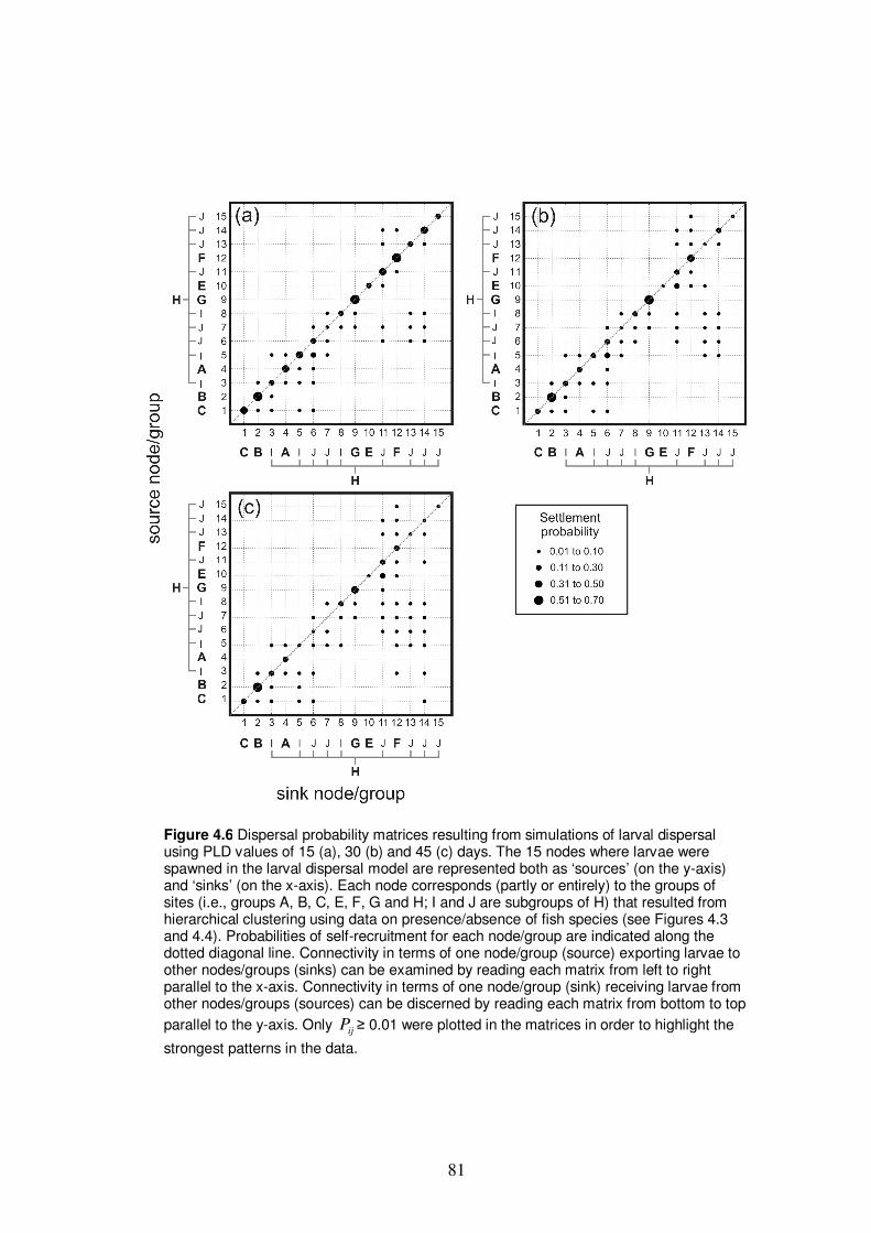
81
Figure 4.6 Dispersal probability matrices resulting from simulations of larval dispersal using PLD values of 15 (a), 30 (b) and 45 (c) days. The 15 nodes where larvae were spawned in the larval dispersal model are represented both as ‘sources’ (on the y-axis) and ‘sinks’ (on the x-axis). Each node corresponds (partly or entirely) to the groups of sites (i.e., groups A, B, C, E, F, G and H; I and J are subgroups of H) that resulted from hierarchical clustering using data on presence/absence of fish species (see Figures 4.3 and 4.4). Probabilities of self-recruitment for each node/group are indicated along the dotted diagonal line. Connectivity in terms of one node/group (source) exporting larvae to other nodes/groups (sinks) can be examined by reading each matrix from left to right parallel to the x-axis. Connectivity in terms of one node/group (sink) receiving larvae from other nodes/groups (sources) can be discerned by reading each matrix from bottom to top
parallel to the y-axis. Only ijP ≥ 0.01 were plotted in the matrices in order to highlight the
strongest patterns in the data.

82
Figure 4.7 Distances of larval dispersal (mean, modal range and maximal range) from each node according to simulations using the biophysical model. Values are given for the range of PLDs (15, 30 and 45 days) used in simulations. Black bars indicate modal range.
Grey bars indicate maximal range ( ijP ≥ 0.01). For each node, the topmost bars are for
15-day PLD, middle bars for 30-day PLD and bottom bars for 45-day PLD. Each node corresponds (partly or entirely) to the groups of sites (i.e., groups A, B, C, E, F, G and H; I and J are subgroups of H) that resulted from hierarchical clustering using data on presence/absence of fish species (see Figures 4.3 and 4.4).
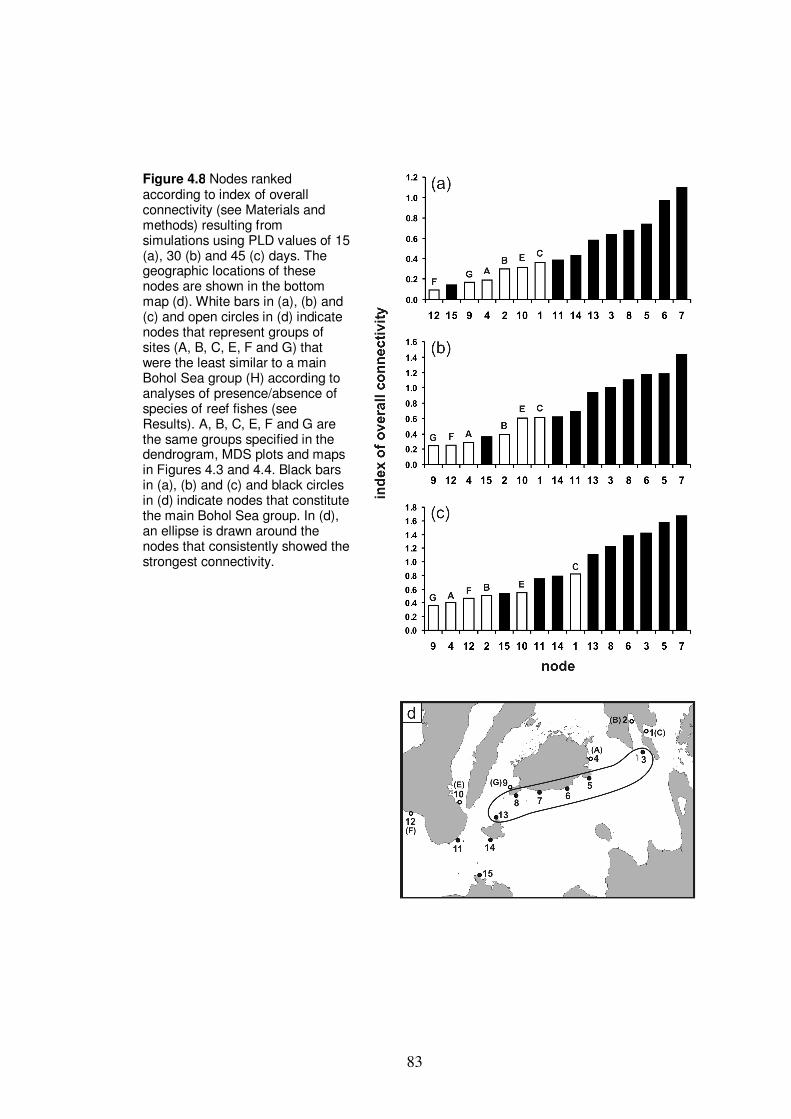
83
Figure 4.8 Nodes ranked according to index of overall connectivity (see Materials and methods) resulting from simulations using PLD values of 15 (a), 30 (b) and 45 (c) days. The geographic locations of these nodes are shown in the bottom map (d). White bars in (a), (b) and (c) and open circles in (d) indicate nodes that represent groups of sites (A, B, C, E, F and G) that were the least similar to a main Bohol Sea group (H) according to analyses of presence/absence of species of reef fishes (see Results). A, B, C, E, F and G are the same groups specified in the dendrogram, MDS plots and maps in Figures 4.3 and 4.4. Black bars in (a), (b) and (c) and black circles in (d) indicate nodes that constitute the main Bohol Sea group. In (d), an ellipse is drawn around the nodes that consistently showed the strongest connectivity.
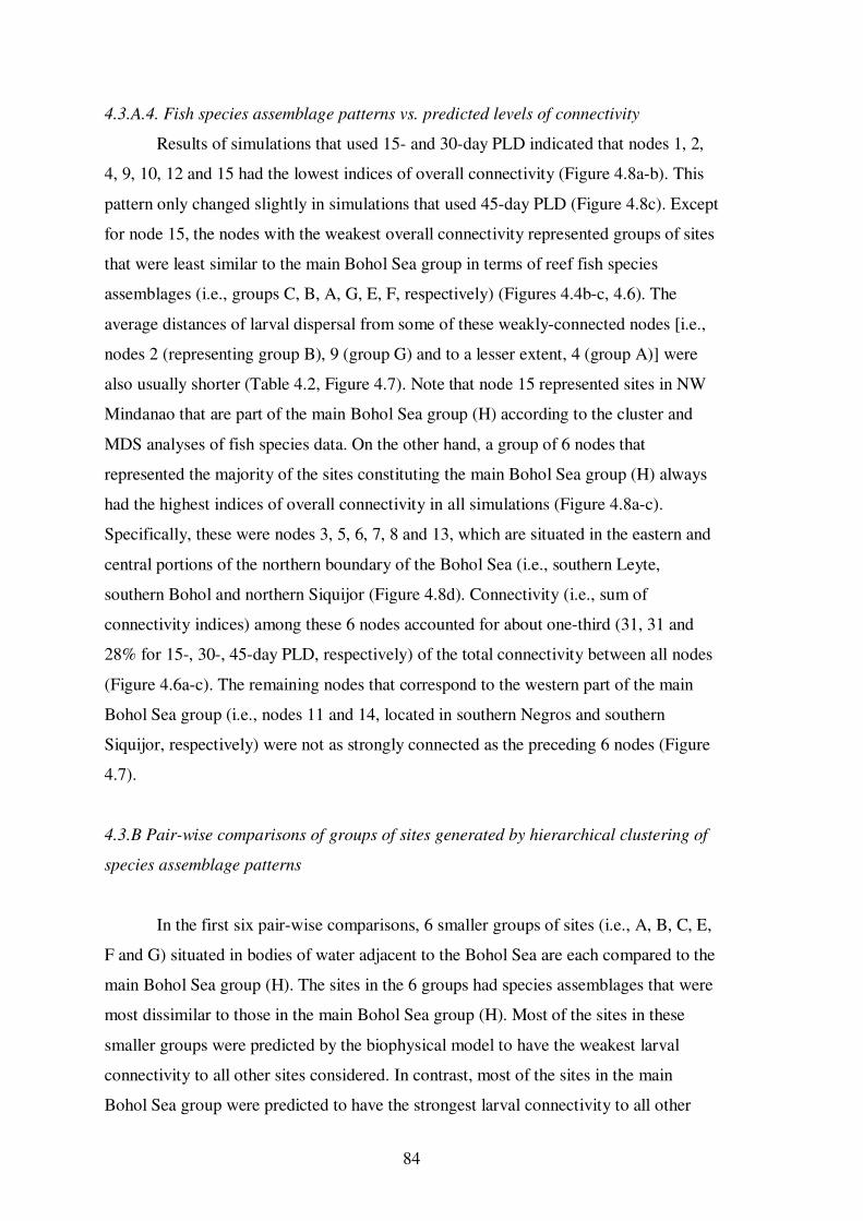
84
4.3.A.4. Fish species assemblage patterns vs. predicted levels of connectivity
Results of simulations that used 15- and 30-day PLD indicated that nodes 1, 2,
4, 9, 10, 12 and 15 had the lowest indices of overall connectivity (Figure 4.8a-b). This
pattern only changed slightly in simulations that used 45-day PLD (Figure 4.8c). Except
for node 15, the nodes with the weakest overall connectivity represented groups of sites
that were least similar to the main Bohol Sea group in terms of reef fish species
assemblages (i.e., groups C, B, A, G, E, F, respectively) (Figures 4.4b-c, 4.6). The
average distances of larval dispersal from some of these weakly-connected nodes [i.e.,
nodes 2 (representing group B), 9 (group G) and to a lesser extent, 4 (group A)] were
also usually shorter (Table 4.2, Figure 4.7). Note that node 15 represented sites in NW
Mindanao that are part of the main Bohol Sea group (H) according to the cluster and
MDS analyses of fish species data. On the other hand, a group of 6 nodes that
represented the majority of the sites constituting the main Bohol Sea group (H) always
had the highest indices of overall connectivity in all simulations (Figure 4.8a-c).
Specifically, these were nodes 3, 5, 6, 7, 8 and 13, which are situated in the eastern and
central portions of the northern boundary of the Bohol Sea (i.e., southern Leyte,
southern Bohol and northern Siquijor (Figure 4.8d). Connectivity (i.e., sum of
connectivity indices) among these 6 nodes accounted for about one-third (31, 31 and
28% for 15-, 30-, 45-day PLD, respectively) of the total connectivity between all nodes
(Figure 4.6a-c). The remaining nodes that correspond to the western part of the main
Bohol Sea group (i.e., nodes 11 and 14, located in southern Negros and southern
Siquijor, respectively) were not as strongly connected as the preceding 6 nodes (Figure
4.7).
4.3.B Pair-wise comparisons of groups of sites generated by hierarchical clustering of
species assemblage patterns
In the first six pair-wise comparisons, 6 smaller groups of sites (i.e., A, B, C, E,
F and G) situated in bodies of water adjacent to the Bohol Sea are each compared to the
main Bohol Sea group (H). The sites in the 6 groups had species assemblages that were
most dissimilar to those in the main Bohol Sea group (H). Most of the sites in these
smaller groups were predicted by the biophysical model to have the weakest larval
connectivity to all other sites considered. In contrast, most of the sites in the main
Bohol Sea group were predicted to have the strongest larval connectivity to all other

85
sites considered. In the seventh comparison, two subgroups of the main Bohol Sea
group (I and J) are compared. For each of the 7 pair-wise comparisons the information
needed to infer the presence (or absence) and potential strength of larval connectivity
between groups (e.g., Table 4.1) are reported: predicted strength of larval exchange
between groups, the habitat characteristics of the sites within each group, the similarity
or dissimilarity of the species assemblages between groups and the habitat preferences
of fish species that contributed most to dissimilarity between groups. A summary of
information used to predict the presence and probable extent of larval connectivity is
given in Table 4.4.
Connectivity Index
Groups compared 15-day 30-day 45-day
1. A vs. H (9) 0.18 15% 0.25 12% 0.36 15%
2. B vs. H (9) 0.18 15% 0.27 13% 0.38 16%
3. C vs. H (9) 0.24 20% 0.46 22% 0.65 27%
4. E vs. H (9) 0.30 24% 0.58 28% 0.49 21%
5. F vs. H (9) 0.08 7% 0.23 11% 0.39 16%
6. G vs. H (9) 0.16 13% 0.23 11% 0.34 14%
7. I vs. J (20) 1.23 2.06 2.38
I vs. J (9 highest) 1.04 85% 1.64 80% 1.72 72%
Table 4.2 Predicted levels of connectivity between 6 groups (A, B, C, E, F and G) and the major Bohol Sea group (H) (1. to 6.) and between two subgroups (I vs. J) of the main Bohol Sea group (7.) (see Figures 4.3 and 4.4 for geographic location of the different groups). Index values are also expressed as % of the highest connectivity index recorded in the study for each PLD. Predictions were based on results of simulations using the biophysical model. For the first six comparisons, connectivity indices were summed for all 9 possible connections (indicated in parentheses) between the nodes in the model. Connectivity indices for the seventh comparison were computed for all 20 possible connections between nodes and for the 9 connections that had the highest index values.

86
4.3.B.1 Group A vs. Group H
Group A comprised 4 sites in southeastern Bohol. Two sites were situated on
fringing reefs within a small bay (Cogtong Bay) while the other two sites were located
on two shoals just outside the mouth of the bay facing the Bohol-Leyte channel (Figure
4.4). The predicted levels of connectivity between groups A and H (regardless of
direction) were some of the lowest among all the pairs of groups compared (Table 4.2).
Connectivity between groups A and H ( ijP ≥ 0.01) were mostly via export of larvae
from group A (node 4) to only two (out of nine) nodes in group H (nodes 5 and 6), and
import of larvae to group A from only two nodes in group H (nodes 3 and 5) (Figures
4.1c, 4.4, 4.6). The sites in group A comprised two types of habitat. The first had a
moderate degree of embayment and was not dominated by any particular benthic
component (i.e., the 2 sites in Cogtong Bay). The second had a high % cover of sand
i.e., the 2 sites situated on shoals) (Figure 4.5b). In contrast, the sites in group H
comprised a broad range of habitat types, including live hard coral-, sand-, rock-, and
macroalgae/seagrass (Figure 4.5c). Analysis using SIMPER indicated that 122 species
of reef fish accounted for ~90% of the dissimilarity between groups A and H (Table
4.3; Appendix 4.2). Of this set of species, only 1 species was unique to group A. Sixty
species (accounting for 49.5% of dissimilarity) were unique to group H. Sixty-one
species were shared by the two groups but most (77%) of these species were more
frequently present in group H. A higher proportion of the species associated with group
A prefer habitats that are more sheltered from winds and wave action, rocky and/or had
more of the substrate types classified as ‘others’ (i.e., seagrass). In contrast, a higher
proportion of the species associated with group H tended to prefer habitats that were
more exposed to winds and wave action (Figure 4.9). The habitat preferences of species
associated with group H remained consistent across all comparisons and will not be
repeated in the succeeding comparisons.
4.3.B.2 Group B vs. Group H
Group B comprised 2 sites in Sogod Bay in southern Leyte (Figure 4.4). The
predicted levels of larval connectivity between groups B and H were also among the
lowest in the study (Table 4.2). Connectivity between groups B and H ( ijP ≥ 0.01) were
mostly through export of larvae from group B (node 2) to only two nodes located in the
eastern portion of group H (nodes 3 and 5), and import to group B from only one node
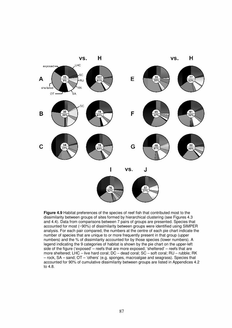
87
Figure 4.9 Habitat preferences of the species of reef fish that contributed most to the dissimilarity between groups of sites formed by hierarchical clustering (see Figures 4.3 and 4.4). Data from comparisons between 7 pairs of groups are presented. Species that accounted for most (~90%) of dissimilarity between groups were identified using SIMPER analysis. For each pair compared, the numbers at the centre of each pie chart indicate the number of species that are unique to or more frequently present in that group (upper numbers) and the % of dissimilarity accounted for by those species (lower numbers). A legend indicating the 9 categories of habitat is shown by the pie chart on the upper-left side of the figure (‘exposed’ – reefs that are more exposed; ‘sheltered’ – reefs that are more sheltered; LHC – live hard coral; DC – dead coral; SC – soft coral; RU – rubble; RK – rock, SA – sand; OT – ‘others’ (e.g. sponges, macroalgae and seagrass). Species that accounted for 90% of cumulative dissimilarity between groups are listed in Appendices 4.2 to 4.8.
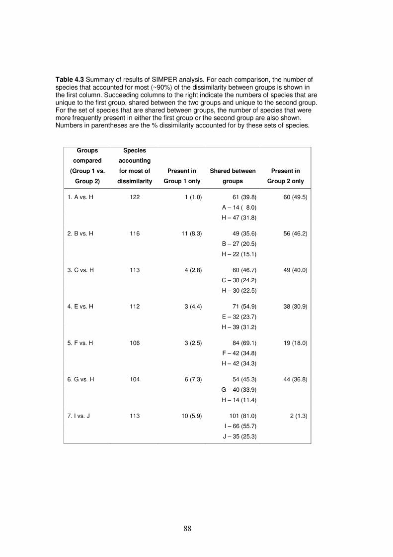
88
Groups
compared
(Group 1 vs.
Group 2)
Species
accounting
for most of
dissimilarity
Present in
Group 1 only
Shared between
groups
Present in
Group 2 only
1. A vs. H 122 1 (1.0) 61 (39.8) 60 (49.5)
A – 14 ( 8.0)
H – 47 (31.8)
2. B vs. H 116 11 (8.3) 49 (35.6) 56 (46.2)
B – 27 (20.5)
H – 22 (15.1)
3. C vs. H 113 4 (2.8) 60 (46.7) 49 (40.0)
C – 30 (24.2)
H – 30 (22.5)
4. E vs. H 112 3 (4.4) 71 (54.9) 38 (30.9)
E – 32 (23.7)
H – 39 (31.2)
5. F vs. H 106 3 (2.5) 84 (69.1) 19 (18.0)
F – 42 (34.8)
H – 42 (34.3)
6. G vs. H 104 6 (7.3) 54 (45.3) 44 (36.8)
G – 40 (33.9)
H – 14 (11.4)
7. I vs. J 113 10 (5.9) 101 (81.0) 2 (1.3)
I – 66 (55.7)
J – 35 (25.3)
Table 4.3 Summary of results of SIMPER analysis. For each comparison, the number of species that accounted for most (~90%) of the dissimilarity between groups is shown in the first column. Succeeding columns to the right indicate the numbers of species that are unique to the first group, shared between the two groups and unique to the second group. For the set of species that are shared between groups, the number of species that were more frequently present in either the first group or the second group are also shown. Numbers in parentheses are the % dissimilarity accounted for by these sets of species.

89
in group H (node 3) (Figure 4.1c, 4.4, 4.6). Sites in group B encompassed a relatively
narrow range of habitat types characterised by high degree of embayment and high %
cover of soft coral, rock or sand (Figure 4.5b). Analysis using SIMPER indicated that
116 species of reef fish accounted for ~90% of the dissimilarity between groups B and
H (Table 4.3; Appendix 4.3). Of this set of species, 11 species (accounting for 8.3% of
dissimilarity) were unique to group B. Fifty-six species (accounting for 46.2% of
dissimilarity) were unique to group H. Forty-nine species were shared by the two
groups, 55% of which were more frequently present in group B. A higher proportion of
the species associated with group B prefer more sheltered and/or rocky habitats (Figure
4.9).
4.3.B.3 Group C vs. Group H
Group C comprised 2 sites in Cabalian Bay, also in southern Leyte (Figure 4.4).
The predicted levels of larval connectivity between groups C and H were low for larvae
with a PLD of 15 days and moderate for larvae with PLD of 30 to 45 days (Table 4.2).
Most of the larval exchange between groups C and H ( ijP ≥ 0.01) were exclusively via
export from group C (node 1) to only 3-4 nodes found mostly in the eastern part of
group H (nodes 3, 5 and 6 for 15- and 30-day PLD; nodes 3, 5, 6 and 14 for 45-day
PLD) (Figure 4.1c, 4.4, 4.6). Sites in group C encompassed a relatively narrow range of
habitat types characterised by a high degree of embayment and moderate to high %
cover of live hard coral (Figure 4.5b). Analysis using SIMPER indicated that 113
species of reef fish accounted for ~90% of the dissimilarity between groups C and H
(Table 4.3; Appendix 4.4). Of these species, 34 (accounting for 29% of dissimilarity)
were unique to or more frequently present in group C. The rest (79 species that
accounted for 63% of dissimilarity) were unique to or more frequently present in group
H. Only 4 species (which accounted for 2.8% of dissimilarity) were unique to group C.
Forty-nine species (accounting for 40.0% of dissimilarity) were unique to group H.
Sixty species were shared by the two groups, 50% of which were more frequently
present in group C and the other 50% more frequently present in group H. The habitat
preferences of species associated with group C did not markedly differ from that of
species associated with group H (Figure 4.9).

90
4.3.B.4 Group E vs. Group H
Group E comprised 3 sites in southeastern Negros, facing Tañon Strait (Figure
4.4). The predicted levels of connectivity between groups E and H were weak (Table
4.2). Larval connectivity between groups E and H ( ijP ≥ 0.01) was exclusively via
larval export from group E (node 10) to just 1-2 nodes located in the western part of
group H (node 11 for 15- and 45-day PLD; nodes 11 and 13 for 30-day PLD) (Figure
4.1c, 4.4, 4.6). Sites within group E had a broad range of habitat types, including reefs
with high % cover of live hard coral, dead coral, rubble and/or substrate types classified
as ‘others’ (i.e., macroalgae and seagrass) (Figure 4.5c). Analysis using SIMPER
indicated that 112 species of reef fish accounted for ~90% of the dissimilarity between
groups E and H (Table 4.3; Appendix 4.5). Of this set of species, only 3 species
(accounting for 4.4% of dissimilarity) were unique to group E. Thirty-eight species
(accounting for 31.1% of dissimilarity) were unique to group H. Seventy-one species
were shared by the two groups, 55% of which were more frequently present in group H.
A higher proportion of the species associated with group E prefer more sheltered and/or
rocky habitats (Figure 4.9).
4.3.B.5 Group F vs. Group H
Group F comprised 4 sites. Two sites are situated in southern Negros, facing
Negros-Mindanao strait, which connects the Bohol Sea to the Sulu Sea (Figure 4.4).
The two other sites are situated in southwestern Negros, facing the Sulu Sea (Figure
4.4). The predicted levels of larval connectivity between groups F and H were among
the lowest recorded in this study (Table 4.2). Connectivity between groups F and H ( ijP
≥ 0.01) were exclusively via import of larvae to group F (node 12) from 2 to all of the 9
nodes within group H (nodes 11 and 14 for 15-day PLD; nodes 11, 13, 14, 15 for 30-
day PLD; and nodes 3, 5, 6, 7, 8, 11, 13, 14, 15 for 45-day PLD). Sites within group F
had a broad range of habitat types, which included reefs that are not embayed, with
moderate degrees of embayment, higher % cover of live hard coral, dead coral and/or
rock (Figure 4.5c). Analysis using SIMPER indicated that 106 species of reef fish
accounted for ~90% of the dissimilarity between groups F and H (Table 4.3; Appendix
4.6). Of this set of species, only 3 species (accounting for 2.5% of dissimilarity) were
unique to group F. Only 19 species (accounting for 18.0% of dissimilarity) were unique
to group H. Eighty-four species were shared by the two groups, 50% of which were

91
more frequently present in group F and the other 50% more frequently present in group
H. A higher proportion of the species associated with group F prefer habitats that are
more exposed and/or have live hard coral (Figure 4.9). The proportion of species that
prefer more sheltered habitats did not differ between groups F and H (Figure 4.9).
4.3.B.6 Group G vs. Group H
Group G comprised 2 sites on fringing reefs in southeastern Bohol (northern
Panglao Is.), facing the Cebu-Bohol channel (Figure 4.4). The predicted levels of
connectivity between groups G and H were among the lowest recorded in this study
(Table 4.2). Larval connectivity between groups G and H ( ijP ≥ 0.01) was almost
exclusively via import of larvae to group G (node 9) from two nodes in group H (nodes
7 and 8 for all PLD values) (Figure 4.6). The only potentially significant export of
larvae by group G to group H was to node 11 (45-day PLD), which is situated in the
western part of group H (Figure 4.6). Sites within group G had a very narrow range of
habitat types characterised by higher % cover of rubble and moderate % cover of live
hard coral (Figure 4.5c). Analysis using SIMPER indicated that 104 species of reef fish
accounted for ~90% of the dissimilarity between groups G and H (Table 4.3; Appendix
4.7). Of this set of species, only 6 species (accounting for 7.3% of dissimilarity) were
unique to group G. Forty-four species (accounting for 36.8% of dissimilarity) were
unique to group H. Fifty-four species were shared by the two groups, most (77%) of
which were more frequently present in group G. A lower proportion of the species
associated with group G prefer habitats that are more exposed but a greater proportion
prefer sandy or seagrass-dominated habitats (the latter was classified as ‘others’ in
Figure 4.9). The proportion of species that prefer more sheltered habitats did not differ
between groups G and H (Figure 4.9).
4.3.B.7 Group I vs. Group J
Groups I and J are the two overlapping subgroups of the main Bohol Sea group
(H) that separate at 73% similarity (Figures 4.3, 4.4). Most of the sites in group I are
situated on the eastern side of the Bohol Sea (13 sites in Leyte and Bohol), while most
of the sites in group J are on the western side (29 sites in Bohol, Siquijor, Negros and
NW Mindanao) (Figure 4.4). The general direction of predicted larval exchange among
the nodes situated in the Bohol Sea is from east to west (see Section 4.3.A.3). The

92
simulations indicated that export of larvae from group I to group J was more frequent
than vice-versa (Figure 4.6). The predicted levels of larval connectivity between groups
I and J were the highest among all the pairs of groups compared in this study (Table
4.2). Considering all of the possible connections (20) between the nodes that represent
groups I and J, larval connectivity between groups I and J were 1.9 to 15.5 times higher
(depending on PLD) than connectivity between any of the 6 smaller groups and the
main Bohol Sea group (H in Table 4.2). Limiting it to the same number of potential
connections between nodes as in the previous comparisons (9 nodes with highest index
values), the levels of connectivity between groups I and J were still 1.6 to 13.1 times
higher (Table 4.2). The sites within group I had a wide range of habitat types, including
reefs that are not embayed, with moderate degrees of embayment, higher % cover of
live hard coral, rock and/or sand (Figure 4.5c). The sites in group J, on the other hand,
had the broadest possible range of habitat types (similar to group H). Analysis using
SIMPER indicated that 113 species of reef fish accounted for ~90% of the dissimilarity
between groups I and J (Table 4.3; Appendix 4.8). The majority of these species (101
species or 89%) were shared between the two groups. However, 65% of the species that
were common to the two groups (66 species accounting for 55.7% of dissimilarity)
were more frequently present in the eastern group (I). Ten species were unique to the
eastern group (I), while only 2 species were exclusive to the western group (J). The
habitat preferences of species associated with group I and group J did not greatly differ
in terms of preference for exposed and sheltered habitats (Figure 4.9).
4.4 Discussion
The objective of this study was to determine the extent of potential larval
connectivity among local populations of coral reef fishes by examining species
assemblage patterns across multiple sites and modelling the probabilities of larval
exchange between these sites. The spatial patterns of species assemblages and predicted
larval exchange were complementary. Taken together, the results from the two
approaches suggested the presence of significant larval connectivity among populations
situated in an area of the Bohol Sea that is influenced by a westward mainstream
current for 6 months of the year. These results also indicated that populations spatially
isolated from this dominant current are not strongly connected by larval exchange to the
populations in the main Bohol Sea. The larval dispersal simulations showed that the

93
Groups compared
Predicted level of larval exchange
Measured habitat characteristics
Measured species assemblage
structure/ Habitat preferences of species
Conclusions and supporting ideas
A vs. H Weak - A exporting to or importing from only 2 (of 9) nodes in H
Different - A = high % cover of sand or slightly embayed; H = broad range of habitat types
Dissimilar - Groups distinguished at ~45% similarity - More species associated with A prefer sheltered (e.g. embayed) habitats
Connectivity likely to be weak - Currents in the vicinity of A (Bohol-Leyte channel) are weaker and isolated from dominant current in the main Bohol Sea - Habitats in A different from most habitats in H - Species assemblages in A could also be influenced by populations in adjacent internal seas (Visayan/Camotes seas)
B vs. H Weak - B exporting to only 2 nodes or importing from only 1 node in H
Different - B = highly embayed, high % cover of sand, soft coral or rock; H = broad range of habitat types
Dissimilar - Groups distinguished at ~56% similarity - More species associated with B prefer sheltered (e.g. embayed) habitats
Connectivity likely to be weak - Currents in the vicinity of B (within Sogod Bay) are weaker and isolated from dominant current in the main Bohol Sea - Habitats in B different from most habitats in H
C vs. H Weak for shorter PLD, moderate for longer PLD
- Unidirectional larval supply: C exporting mostly to 3-4 nodes in eastern part of H
Different - C = highly embayed, moderate to high % cover of live hard coral, similar to many sites in H
Dissimilar - Groups distinguished at ~59% similarity - Habitat preferences of species associated with C were not very different from those associated with H
Connectivity likely to be weak - Currents in the vicinity of C (within Cabalian Bay) are weaker and isolated from dominant current in the main Bohol Sea - Degree of larval exchange may also be limited by strong (unidirectional) current entering Bohol Sea through Surigao Strait - Species assemblages in C may also be influenced by Pacific (eastern Philippine) populations
Table 4.4 Summary of information required to infer the presence and probable extent of larval connectivity between sampling sites. Information on predicted levels of larval exchange, measured habitat characteristics, measured species assemblage structure and habitat preferences of species for each of 7 pairs of site groups are summarised. Conclusions about larval connectivity and the ideas supporting these conclusions are found in the last column.

94
E vs. H Weak - Unidirectional larval supply: E exporting mostly to 1-2 nodes in western part of H
More similarities (larger overlap) in habitat types between the two groups - E = high % cover of live hard coral, dead coral, rubble and/or macroalgae and seagrass), similar to many H sites
Dissimilar - Groups distinguished at ~64% similarity - More species associated with E prefer sheltered (e.g. embayed) habitats
Connectivity likely to be weak and limited to only a few sites in western part of H - Degree of larval exchange may also be limited by strong (unidirectional) southward current passing through Tañon Strait - Species assemblages in E could also be influenced by populations in an adjacent internal sea (i.e., Visayan Sea)
F vs. H Weak - Unidirectional larval supply: 2 to 9 nodes in H (depending on PLD) exporting to F
More similarities (larger overlap) in habitat types between the two groups - F = higher % cover of live hard coral, dead coral and/or rock, similar to many H sites
Dissimilar - Groups distinguished at ~66% similarity - More species associated with F prefer exposed habitats but proportion of species that prefer sheltered habitats did not differ between two groups
Connectivity likely to be weak - Degree of larval exchange may be limited by strong (unidirectional) current exiting Bohol Sea through Negros- Mindanao Strait - Species assemblages in F may also be influenced by populations in the Sulu Sea
G vs. H Weak - Larval supply almost exclusively unidirectional; only 2 neighbouring nodes in H exporting larvae to G
Different - G = high % cover of rubble and moderate % cover of live hard coral; H = broad range of habitat types
Dissimilar - Groups distinguished at ~68% similarity - Fewer species associated with G prefer exposed habitats but more species prefer sandy or seagrass- dominated habitats
Connectivity likely to be weak - Currents in the vicinity of G (Cebu-Bohol channel) are weaker and isolated from dominant current in the Bohol Sea - Habitats in G different from most habitats in H - Species assemblages in G could also be influenced by populations in adjacent internal seas (i.e., Camotes and Visayan seas)
I vs. J Strong - Mostly via export from I to J (westward) than the opposite
More similarities (larger overlap) in habitat types between the two groups - I = higher % cover of live hard coral, rock and/or sand, similar to many sites in J
Similar - Groups distinguished at ~73% similarity - Habitat preferences of species associated with each group did not greatly differ
Connectivity likely to be strong - Presence of dominant westward current and high degree of similarity in habitat types between the two groups - Previous work by Ablan (2005, 2006) suggesting east to west genetic sub-structuring in 2 species of reef fish within Bohol Sea
Table 4.4. Continued.
95
direction of potential larval connectivity within the Bohol Sea is predominantly
westward. This is consistent with the known general direction of the mainstream
current throughout the year.
The assessment of the potential effects of larval supply and local habitat on the
species assemblage patterns reinforced the notion of significant population connectivity
within the Bohol Sea (Table 4.4). Among all the comparisons between groups of sites,
the probable presence of high levels of connectivity can be concluded only for the
eastern and western subgroups of the Bohol Sea (i.e., Table 4.4, I vs. J tend to reflect
Case 1 in Table 4.1). Compared to other pairs of groups, these two subgroups were
predicted to have the highest rates of larval exchange and had substantial overlap in the
types of habitat they encompassed. The combination of these two factors may
contribute significantly to the higher level of species assemblage similarity (~68-73%)
of the two subgroups. Similar types of habitat between the two subgroups would
facilitate recruitment of larvae dispersing from eastern to western populations. Further
support for the conclusion that populations in the Bohol Sea are likely to be more
strongly connected by dispersal and recruitment of larvae is indicated by the set of
species that differentiated the two subgroups. The majority (89%) of this set of species
was shared by the two subgroups. However, most (65%) of the shared species were
more frequently present in the eastern subgroup (I) than in the western subgroup (J).
This was the case despite the narrower range of habitat types and fewer sampling sites
that were included in the eastern subgroup. Also, there were more species unique to the
eastern subgroup (10 species) than the western subgroup (2 species). Such patterns are
consistent with the westward direction of potential larval connectivity between the
subgroups, i.e., for individual species, the probability of connectivity is expected to
decrease downstream of the dominant current. The habitat preferences of the species
associated with each subgroup did not greatly differ, which is to be expected if the two
subgroups have many types of habitat in common.
Ablan (2005, 2006) used microsatellite DNA markers to determine potential
patterns of connectivity among several populations of two species of reef fish
(Dascyllus trimaculatus and Pterocaesio pisang) across the Bohol Sea. The results of
her study suggested eastern and western groups of reef fish populations in this area,
roughly similar to the two subgroups (I and J) of the main Bohol Sea group that were
found in the present study. However, caution must be exercised when comparing the
results of the two studies. Ablan (2006) suggested that the eastern and western groups

96
she found were not strongly connected to each other by larval dispersal, which
contradicts the conclusions of the present study. The contrasting conclusions of the two
studies about potential connectivity in the Bohol Sea were probably due to differences
in the spatial scales at which populations of reef fishes were sampled and the locations
of these populations. The study by Ablan had a very limited number of sites (7 at most)
to provide a clear picture of probable ecological-scale larval connectivity across a 300
km wide area. Furthermore, the sites she sampled were mostly offshore islands (e.g.
Apo, Sumilon, Balicasag, Selinog, Mantigue; see Figure 4.1b), which were not included
in the present study. More importantly, two of the sites she sampled are situated outside
of the area that was sampled in the present study (i.e., Dinagat Is. and Mantigue Is.;
Figure 4.1b). A possible explanation for weak connectivity between the eastern and
western regions of the Bohol Sea for some species or sites is the presence of mesoscale
eddies that form at different times of the year (Figure 4.2). Such eddies may limit the
westward dispersal of larvae. Nevertheless, Ablan (2005, 2006) showed that ecological-
scale larval connectivity may be present in the Bohol Sea within spatial scales of 10’s
of km for the sites that she sampled (e.g., between Apo, Sumilon, and Balicasag
islands; Figure 4.1b). Significant self-recruitment at very small spatial scales (< 1 km)
may also be present at these sites (Ablan 2005, 2006).
The results of the present study suggested that the species assemblage patterns
could be partly explained by a combination of several habitat variables, particularly
degree of embayment, % cover of sand and % cover of rubble. These habitat variables
could be more important in differentiating the species assemblages of sites situated
within bays and two channels (i.e., Bohol-Leyte and Cebu-Bohol channels) from those
found in other sites, especially the many sites that comprised the main Bohol Sea group.
Two of the sites in group A and all of the sites in groups B and C (including group B-C)
were all situated within bays (i.e., Cogtong, Sogod and Cabalian bays, respectively).
Fish assemblages on reefs that are sheltered within bays tend to differ in community
structure and have lower species richness and diversity compared to assemblages found
on more exposed reefs outside of bays (Friedlander et al. 2003). A probable effect of
embayment was also indicated by the greater proportion of the species associated with
groups A and B (but, interestingly, not the species associated with C) preferring more
sheltered habitats compared to the species associated with the Bohol Sea group. The
main Bohol Sea group, in contrast, had a higher proportion of species that preferred
more exposed habitats probably because the sites that composed this group are mostly
97
found along coastlines exposed to winds (i.e., southwest and northeast monsoons) and
wave action. High % cover of sand could be an important factor in differentiating the
species assemblages in two other sites that composed group A, which are situated on
shoals in the Bohol-Leyte channel. Higher % cover of sand usually correlates with
lower structural complexity of reefs in the region that was studied (Abesamis et al.
2006b). Lower structural complexity, in turn, is commonly associated with lower
species richness and abundance of coral reef fishes (e.g., Carpenter et al. 1981). Note,
however, that the two sites in group A with sandy habitat were more similar in species
assemblage to the two other sites in the same group situated in Cogtong Bay, than any
other site in the Bohol Sea group with sandy habitat (Figures 4.3 and 4.5). Lastly, the
results suggested that higher % cover of rubble could be important in differentiating the
species assemblages of the two sites in group G, which are situated in the Cebu-Bohol
channel. However, the set of species associated with group G did not show a strong
preference for rubble-dominated habitats. Also, among the three potentially influential
habitat variables, % cover of rubble had the lowest correlation to the species
assemblage patterns.
Differentiation of the species assemblages in the sites belonging to groups A, B,
C and G could be driven to some extent by dissimilarities in habitat, but the larval
dispersal simulations indicated low levels of larval exchange between these groups and
the Bohol Sea group. Results of comparisons of groups A-C and G with group H (Table
4.4) reflect Case 4 in Table 4.1. Thus it is likely that groups A-C and G are weakly
connected by larval exchange to the populations in the Bohol Sea. No other studies are
available to independently validate the results of the larval dispersal simulations.
However, the results of the simulations with respect to groups A-C and G are plausible
representations of potential larval exchange based on the sea surface circulation
patterns indicated by the NLOM (Figure 4.2). Throughout the year, all of the sites in
these weakly-connected groups are situated in areas that appear to be isolated from the
mainstream flow that probably connects populations within the main Bohol Sea (Figure
4.2). The data from NLOM also suggest that the currents in these areas are much
weaker compared to the mainstream current (Figure 4.2). Such conditions would
significantly decrease the probabilities of population connectivity between groups A-C
and G and the main Bohol Sea group. The simulations indicated that the predicted
connectivity between these groups and the Bohol Sea group were usually weaker or
mostly limited to areas that are relatively close (more frequently within 25-125 km)

98
even for the longest PLD tested (45 days) (Table 4.2, Figures 4.6, 4.7). It should be
noted that for the sites situated within bays, the effect of embayment as a habitat factor
is likely to be confounded by its effect as a physical feature. Degree of embayment
could also limit larval exchange due to potential differences in circulation patterns
inside and outside of bays.
Habitat dissimilarity was unlikely to be the most influential factor in
differentiating the species assemblages of the sites in group E in the Tañon Strait and
group F in or close to the Sulu Sea from the species assemblages in the main Bohol Sea
group. Groups E and F included many types of habitat that were similar to the main
Bohol Sea group (Figure 4.5). A more likely reason for the differentiation of the species
assemblages of the sites in groups E and F is limitation of larval exchange with
populations in the Bohol Sea due to the local geographic (or oceanographic) setting.
Results of simulations indicated that the larval connections of groups E and F with the
Bohol Sea group are weak. These potential connections predominantly occur in one
direction only, due to the strong southward current flowing through the Tañon Strait for
group E (towards the Bohol Sea) and the westward current flowing through the Negros-
Mindanao Strait for group F (from Bohol Sea to the Sulu Sea) almost throughout the
year (Figure 4.2). The data from the NLOM suggest that dispersal of larvae in the
directions opposite to the general flow of these strong currents is limited, since it may
occur only during the relatively brief flow reversals associated with the tides. The
results of the comparisons of groups E and F with the Bohol Sea group (H) (Table 4.4)
are more similar to Case 3 in Table 4.1. Thus, it is likely that populations in groups E
and F are only weakly connected by larval exchange to the populations in the main
Bohol Sea. In addition, the local geographic setting suggests that differentiation of the
species assemblages of groups E and F could also be partly due to potential connections
of the populations within these two groups with other populations outside of the Bohol
Sea (i.e., Visayan Sea populations for group E; Sulu Sea populations for group F). Such
a consequence of the local geographic setting may also be partially responsible for the
differentiation of species assemblages in group C (i.e., potential connections with
Pacific populations) and groups A and G (i.e., potential connections with Visayan Sea
and/or Camotes Sea populations).
The findings of this study improve the current understanding of larval
connectivity of fish populations on coral reefs within the Bohol Sea, in particular, and
also in archipelagic regions, in general. For populations in the Bohol Sea, higher levels
99
of ecologically-relevant larval connectivity may occur more often within ~25 km of
their potential source populations (Figures 4.6, 4.7). Lower levels of connectivity may
be expected at greater distances, up to 100-275 km away from potential source
populations, depending on geographic location (Figure 4.7). These spatial scales of
potential demographic connectivity in reef fishes are consistent with the findings of
previous work by Ablan (2005, 2006) in the Bohol Sea and others elsewhere (James et
al. 2002; Bode et al. 2006; Cowen et al. 2006; Jones et al. 2009; Planes et al. 2009;
Christie et al. 2010; Saenz-Agudelo et al. 2011). In the absence of detailed empirical
measurements of population connectivity between reserves and non-reserves across the
entire Bohol Sea region, these initial estimates of distances of demographically-
significant larval dispersal can be used as ‘rules of thumb’ in efforts to optimise reserve
network design. The limited distances for significant levels of larval exchange between
populations also indicate a greater chance for older reserves to subsidise recruitment to
nearby fished areas (< 25 km away) and for many neighbouring reserves to interact,
potentially resulting in synergistic positive effects (Chapter 5). These possibilities place
the small (< 1 km2) but numerous and closely-spaced (mostly within 1-5 km of each
other) reserves in the Bohol Sea in a more positive light given the concern that the
majority of these reserves are not protecting sufficient areas of coral reef to achieve
conservation goals (McClanahan 1999; Roberts et al. 2002; Weeks et al. 2010a). Weeks
et al. (2010a) also pointed out that ecologically-relevant larval connectivity between
existing reserves in the Philippines is likely because, on average, many of these
reserves are situated within 10’s of km of each other.
This study showed that broad-scale species assemblage patterns of coral reef
fish may indicate potential larval connectivity within the spatial scales expected for
ecologically-relevant larval dispersal. The spatial scales at which the presence or
absence of larval connectivity inferred from species assemblage patterns in this study
were smaller compared to the study done by Roberts (1991) in the Red Sea but similar
to the study done by Williams et al. (1986) across the continental shelf of the Great
Barrier Reef. Patterns of larval connectivity among population on coral reefs are likely
to be strongly influenced by the local geographic setting (Jones et al. 2009). In the case
of the Bohol Sea region, patterns of larval connectivity among reef fish populations are
probably heavily influenced by the local hydrodynamic regime, including how current
patterns are modified by many islands, the coastline features of larger islands (e.g.,
bays), bathymetric features and monsoon winds. However, the results of this study

100
indicate that the insights on probable larval connectivity gained from species
assemblage patterns will only be meaningful if the effects of local habitat on species
assemblage patterns and the probable patterns of larval exchange are also assessed.
The main contribution of this study was the creation of a working framework
for testing hypotheses about population connectivity at the regional (100’s of km, inter-
island) scale. Such a framework would be invaluable for the application of more direct
but also more expensive and labour-intensive methods (e.g. parentage analysis or
tagging of larval otoliths) to empirically test larval connectivity between specific local
populations of reef fishes in the region. Results of this study also indicate that the most
significant levels of demographically-relevant connectivity occur within more limited
spatial scales (a few 10’s of km). In the final study (Chapter 5), two of the most critical
expectations from reserve networks are tested in some of the oldest and most studied
reserves in the Bohol Sea: recruitment subsidy by reserves to surrounding fished areas
and reserve to reserve connectivity.

101
Chapter 5
Potential recruitment subsidy and connectivity of small no-take
marine reserves in the central Philippines
Abstract. Recruitment subsidy (net larval export) from no-take marine reserves is
widely expected to enhance fisheries but remains highly controversial. Its development,
magnitude and spatial extent will depend upon the patterns of connectivity (larval
exchange) among populations inside and outside reserves. In this study, potential
recruitment subsidy and connectivity of 39 small (< 1 km2) community-based reserves
situated on heavily fished coral reefs in the central Philippines were investigated using
a simple exponential model of population recovery and larval production inside
reserves, coupled with an individual-based larval dispersal model. The 39 reserves
protect only 6% of total reef area. Simulations indicated that a 3.5-fold (~250%)
increase in recruitment to fished areas can result from a 55-fold increase in larval
production by large predatory reef fishes inside reserves if all reserves were
continuously and effectively protected for 20 years. Lower larval production
differentials (3- and 7-fold increases) within the first decade of reserve protection will
bring about much smaller increases (< 21% change) in recruitment. These lower larval
subsidies are likely to at least replace losses in yield due to reserve creation but they are
difficult to detect because of substantial temporal and spatial variation in recruitment.
Results also showed that for the same larval dispersal potential (30-day larval life), the
spatial pattern of recruitment subsidy, the probability of net larval export from reserves
and the probabilities of larval exchange among reserves are influenced more strongly
by local geography and current patterns rather than larval production levels within
individual reserves. Probabilities of self-recruitment within and connectivity between
the small reserves were extremely low (always < 0.03) but the absolute magnitudes of
larval exchange between reserves increased dramatically (up to ~20-fold) with higher
larval production. These findings underscore the importance of protecting reserves over
the long-term (decades) and establishing networks of reserves that are connected by
larval dispersal in order for reserves to provide meaningful recruitment subsidy to
fisheries.

102
5.1 Introduction
It is now well-established that the abundance of organisms targeted by fisheries
can build up inside no-take marine reserves (Roberts and Polunin 1993; Russ 2002;
Gell and Roberts 2003; Halpern and Warner 2003; Lester et al. 2009; Molloy et al
2009; Babcock et al. 2010). However, the effects of reserves beyond their boundaries
remain open to question. Reserves may positively affect surrounding fisheries through
net export of mobile adults (i.e.,‘spillover’). Such effects have been demonstrated (e.g.,
Russ et al. 2004; Abesamis and Russ 2005; Halpern et al. 2010). A much larger
potential benefit to fisheries may come from the net export of pelagic larvae (i.e.,
‘recruitment subsidy’) (Carr and Reed 1993; Sale et al 2005). However, it is still
unclear if recruitment subsidy benefits are realised (Russ 2002; Sale et al 2005). Also,
there is concern about whether such larval subsidies to fisheries will ever be enough to
more than compensate for the losses in yield that may result from the creation of
reserves because of decreased fishing area (Halpern and Warner 2003; Hilborn et al.
2004). At present, the evidence for reserves affecting larval settlement to fished areas is
sparse and limited mainly to sessile invertebrates (Gell and Roberts 2003; Sale et al.
2005; Cudney-Bueno et al. 2009; Pelc et al. 2009, 2010; Christie et al. 2010).
Demonstrating recruitment subsidy from reserves for the multitude of targeted marine
species remains a challenge that is hindered by the same difficulties inherent in the
study of marine larval dispersal, recruitment variation and population connectivity.
Most reserves are smaller than the mean larval dispersal range of the majority of
marine species (Roberts and Hawkins 1997; Shanks et al. 2003; Palumbi 2004; Jones et
al. 2009; Weeks et al. 2010a). Thus, any increase in larval production inside reserves
will almost certainly lead to a proportional increase in recruitment to fished areas (and
other reserves) within the range of larval dispersal (Halpern et al. 2004). Such larval
subsidies are potentially very important in sustaining fisheries especially when most
spawners are found within reserves as opposed to fished areas (Davis 1977, Pelc et al.
2010). Even if larval export from reserves is highly likely, theoretical studies indicate
that large reserves (10’s of km long) with exceptionally high levels of larval production
relative to fished areas may be necessary before recruitment subsidy can be detected
against the noise of natural recruitment fluctuations (Halpern et al. 2004; Pelc et al.
2010). In reality, however, the conversion of large proportions of fishing grounds into
reserves and the successful maintenance of large reserves are more difficult to achieve,

103
particularly in developing countries (Roberts and Hawkins 1997; Russ and Alcala 1999;
Alcala and Russ 2006).
Reserves must be situated in ‘source’ sites in order to effectively enhance
fisheries through recruitment subsidy (Crowder et al. 2000; Russ 2002). This means
that reserves should be established in good quality habitats where the potential for
population growth is higher, resulting in greater build-up of spawning biomass. This
also means that reserves should be located in sites where the probability of export of
larvae far outweighs that of import. Conversely, reserves will be less effective
contributors of larvae if they are situated in ‘sink’ sites where poorer-quality habitat
limits population growth and larval import is greater than export. The potential for
source-sink population dynamics (Pulliam 1998) is likely to be high in coral reefs
because of considerable habitat heterogeneity (Crowder et al. 2000). Furthermore, reef
populations will likely differ in their tendencies to export and import larvae because of
complex hydrodynamic patterns that are typical of coral reef environments (Roberts
1997; James et al. 2002; Bode et al. 2006; Cowen et al. 2006). The implications of
source-sink dynamics to reef populations suggest that situating reserves at source sites
is of utmost importance, while haphazard or random placement of reserves should be
avoided (Crowder et al. 2000). However, the process of establishing reserves is often
more strongly driven by socio-economic considerations and opportunism rather than
scientific understanding of source-sink dynamics (Roberts 2000; Roberts et al. 2003;
Alcala and Russ 2006; McCook et al. 2009). Identifying source and sink sites is time-
consuming or simply not feasible in many situations. On the other hand, there is a view
that sources may be created simply by establishing reserves, with little or no
consideration of source-sink relationships, because spawning biomass inside reserves is
likely to become much greater than fished areas (Roberts 1998, 2000). This possibility
remains largely unexamined.
Field studies of larval dispersal of reef fishes at ecologically relevant scales
have demonstrated significant self-recruitment at the scale of small islands, individual
reefs or reserves (i.e., less than a few kilometres) (Jones et al. 1999; Swearer et al.
1999; Jones et al. 2005; Almany et al. 2007; Planes et al. 2009). While these studies
indicate the potential for populations within reserves to be self-sustaining, the recovery
and persistence of reserve populations may also greatly depend upon larval supply from
elsewhere, either from fished areas or other reserves (Jennings 2000; Roberts 2000;
Planes et al. 2009). In situations where fished areas are heavily exploited, a network of
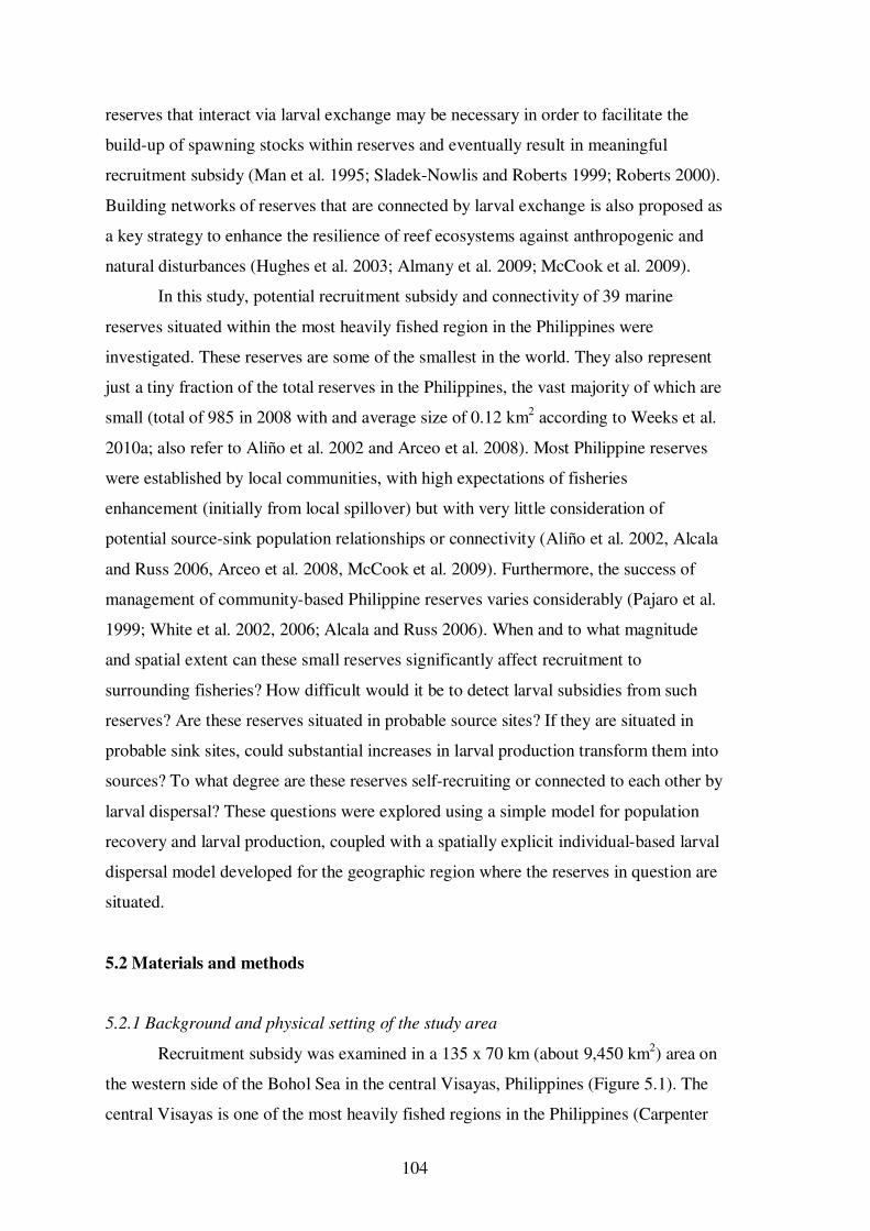
104
reserves that interact via larval exchange may be necessary in order to facilitate the
build-up of spawning stocks within reserves and eventually result in meaningful
recruitment subsidy (Man et al. 1995; Sladek-Nowlis and Roberts 1999; Roberts 2000).
Building networks of reserves that are connected by larval exchange is also proposed as
a key strategy to enhance the resilience of reef ecosystems against anthropogenic and
natural disturbances (Hughes et al. 2003; Almany et al. 2009; McCook et al. 2009).
In this study, potential recruitment subsidy and connectivity of 39 marine
reserves situated within the most heavily fished region in the Philippines were
investigated. These reserves are some of the smallest in the world. They also represent
just a tiny fraction of the total reserves in the Philippines, the vast majority of which are
small (total of 985 in 2008 with and average size of 0.12 km2 according to Weeks et al.
2010a; also refer to Aliño et al. 2002 and Arceo et al. 2008). Most Philippine reserves
were established by local communities, with high expectations of fisheries
enhancement (initially from local spillover) but with very little consideration of
potential source-sink population relationships or connectivity (Aliño et al. 2002, Alcala
and Russ 2006, Arceo et al. 2008, McCook et al. 2009). Furthermore, the success of
management of community-based Philippine reserves varies considerably (Pajaro et al.
1999; White et al. 2002, 2006; Alcala and Russ 2006). When and to what magnitude
and spatial extent can these small reserves significantly affect recruitment to
surrounding fisheries? How difficult would it be to detect larval subsidies from such
reserves? Are these reserves situated in probable source sites? If they are situated in
probable sink sites, could substantial increases in larval production transform them into
sources? To what degree are these reserves self-recruiting or connected to each other by
larval dispersal? These questions were explored using a simple model for population
recovery and larval production, coupled with a spatially explicit individual-based larval
dispersal model developed for the geographic region where the reserves in question are
situated.
5.2 Materials and methods
5.2.1 Background and physical setting of the study area
Recruitment subsidy was examined in a 135 x 70 km (about 9,450 km2) area on
the western side of the Bohol Sea in the central Visayas, Philippines (Figure 5.1). The
central Visayas is one of the most heavily fished regions in the Philippines (Carpenter

105
Figure 5.1 Map of the study area showing the 39 no-take marine reserves. The reserves are numbered according to year of establishment (oldest to newest, see Table 5.1).

106
and Alcala 1977; Burke et al. 2002; Alcala and Russ 2002; Green et al. 2003, 2004;
Lavides et al. 2009; Nañola et al. 2010). The area that was studied included coastlines
of southern Negros and Cebu islands, the entire island of Siquijor and two smaller
islands (<1 km2 in area), namely Apo and Sumilon (Figure 5.1). The total length of
these coastlines is approximately 279 km. Most of the coastlines have coral reefs but
detailed data on the extent of reef and other shallow-water habitats for reef fishes (e.g.,
mangrove, seagrass, rocky and soft-bottom habitats) are lacking. Due to the absence of
fine-scale habitat data, the term ‘reef’ as it is used here broadly refers to coral reefs and
other habitat associated with reefs that are suitable for the breeding of adult reef fishes
and settlement of their larvae.
The study area is bounded by the Tañon Strait to the north, the Bohol Sea and
Cebu-Bohol Strait to the east, the Negros-Mindanao Strait to the south and the Sulu Sea
to the west (Figure 5.1). Data from the U.S. Navy Layered Ocean Model (NLOM)
indicate that the general direction of surface currents in this area is towards the
south/south-west (www7320.nrlssc.navy.mil/global_nlom). These currents are driven
mainly by the southward flow of water through Tañon Strait and westward flow from
the Bohol Sea to the Sulu Sea, exiting through the Negros-Mindanao Strait. However,
actual current patterns are highly complex spatially and exhibit seasonal variation due
to the reversing monsoon winds (Chapter 4; Figure 4.2).
5.2.2 No-take marine reserves
Thirty-nine small (all but one were < 0.5 km2 in area) marine reserves situated
mainly on reef habitat occur within the study area according to a recent census done by
Alcala et al. (2008) (Figure 5.1, Table 5.1). These reserves were established by local
fishing communities with support from their local government units and non-
governmental organisations (Russ and Alcala 1999; White and Vogt 2000; Yambao et
al. 2001; Alcala and Russ 2006; Alcala et al. 2008). For the most part, the placement of
these reserves was not guided by an explicit networking strategy incorporating
connectivity (McCook et al. 2009) but there was some consideration of placing reserves
on good reef habitat (not necessarily prime fishing ground). The reserves vary in size
(0.02 to 0.76 km2), extent of reef habitat, duration of protection (DOP) and
effectiveness of management by the local stakeholders (Table 5.1). Alcala et al. (2008)
found that only 22 of the 39 reserves were functional in ca. 2008, i.e., protection was
reasonably effective since the establishment of the reserve or after a certain point in

107
time. Ten were found to be non-functional, i.e., protection was ineffective or totally
absent. Seven of the reserves were newly-established, i.e., DOP was ≤ 3 years. The two
oldest (since initial establishment) and most studied of these reserves are situated at
Sumilon and Apo islands, which were created in 1974 and 1982, respectively (Table
5.1; Russ 1985; Alcala 1988; White 1988; White and Vogt 2000; Alcala and Russ
2006; Russ and Alcala 2010).
5.2.3 Larval dispersal model
A Lagrangian (particle-tracking) model was developed to simulate dispersal of
reef fish larvae for the entire Bohol Sea (Chapter 4). This model was used in the present
study to examine potential larval exchange between reserves and fished areas that are
found within the study area (Figure 5.1). A detailed description of the spatial domain,
hydrodynamic forcing and larval behavioural parameters of the model are provided in
Chapter 4. However, three key points about how the model was configured for the
present study need to be mentioned. Firstly, it was assumed that reefs were uniformly
distributed along the coastlines encompassed by the study area (Figure 5.1). Secondly,
the reefs found along these coastlines were the only ones designated as sources of
larvae (spawning areas) in the model. Thirdly, the size of each grid cell in the model
was 2.2 x 2.2 km (4.8 km2). This grid cell size is much larger than the individual size of
any of the 39 reserves, which is a limitation of the model due to the very small size of
the reserves (Table 5.1). A reserve may therefore share a grid cell with fished areas and
other reserves. In all, there were 32 reef grid cells that contained reserves. Five of these
had 2 or 3 neighbouring reserves.
5.2.4 Larval production from and recruitment to reserves and fished areas
The reefs in the model were treated as units of reef slope 0.4 km long, parallel to
the coast, and 0.1 km wide, seaward. One unit of reef therefore had a virtual reef slope
area of 0.04 km2 or 40,000 m
2. It was then assumed that each reserve occupied only one
unit of reef. The remaining units were fished areas. The resulting ratio between total
reserve and fished area units was 1:17. This meant that only about 6% of the total
hypothetical reef area in the model was occupied by reserves and 94% was open to
fishing. The assumption that an individual reserve protected only 0.04 km2 of reef can
be justified for the majority (34 or 87%) of the 39 reserves, i.e., those reserves that are

108
Reserve, Island Area (km
2) Habitat
Year Established
DOP until ca. 2008
Fish Abundance
Coral Cover Management Status
Equivalent larval production (DOP)
1. Sumilon Island 0.13 R 1974 (1987) (1995)
13 Medium Fair Functional since 1995 10
2. Apo Island 0.15 R 1982 26 Very high Good Functional 20 3. Tubod, Siquijor 0.09 R 1986 (2004) 4 High Good Functional since 2004 5 4. Tulapos, Siquijor 0.25 R, M, S 1987 21 High Fair Functional 20 5. Caticugan, Siquijor 0.14 R, SB 1989 (2003) 5 Low Poor Functional since 2003 5 6. Poblacion San Jose, Negros
0.05 R, S 1994 14 Low Poor Non-functional = fished
7. Bonbonon, Negros 0.09 R 1995 13 Low Fair Non-functional = fished 8. Andulay, Negros 0.06 R 1996 12 Medium Fair Functional 10 9. Tandayag, Negros 0.06 R 1996 12 High Fair Functional 10 10. Nonoc, Siquijor 0.04 R, SB 1996 (2003) 5 Low Poor Non-functional = fished
11. Candaping B, Siquijor
0.24 R 1996 (2003) 5 Low Fair Functional since 2003 5
12. Cangmating, Negros
0.06 R 1997 11 Very low Fair Non-functional = fished
13. Masaplod Norte, Negros
0.06 R, S 1997 11 Very high Poor Functional 10
14. Polo, Negros 0.02 R, M, S 1998 10 Low Poor Non-functional = fished 15. Taculing/Cangma- lalag, Siquijor
0.13 R, M, S 1998 (2003) 5 Low Poor Non-functional = fished
16. Agan-an, Negros 0.06 R, S 1999 9 Low (2002) Fair Functional 10
17. Bio-os, Negros 0.09 R 1999 9 Medium Good Functional 10 18. Buntis, Negros 0.06 R 2000 8 Low Poor Non-functional = fished
19. North Lipayo, Negros
0.02 R 2000 8 Low Good Functional, but low biomass
5
Table 5.1 List of the 39 reserves situated on reefs within the study area. Types of habitat within reserves include coral reef (R), seagrass (S), mangrove (M) and soft or sandy bottoms (SB). Some reserves were re-established at least once. Years of re-establishment are enclosed in parentheses. Assessments of fish abundance (density or biomass), coral cover and management status were based on Alcala et al. (2008). The last column indicates the estimated larval production, i.e., equivalent to a fished area, 5, 10 or 20-year-old reserve; see Table 5.2 and Materials and methods).

109
20. Maayong Tubig, Negros
0.07 R 2000 8 Medium Poor Functional 10
21. Poblacion 1, Negros 0.09 R, S 2000 8 High Good Functional 10 22. Salag, Negros 0.10 R 2001 7 Low Poor Non-functional = fished 23. Banilad, Negros 0.76 R, S 2001 7 Medium Poor Functional 5
24. Masaplod Sur, Negros
0.06 R 2001 7 Very high Poor Functional 10
25. Pasil, Cebu 0.10 R 2002 6 Very high Fair Functional 5 26. Lutoban, Negros 0.10 R 2002 6 Low Fair to Poor Functional 5 27. Colase, Cebu 0.16 R 2002 6 High Fair Functional 5 28. Minalulan, Siquijor 0.12 R, SB 2003 5 Very low Fair Non-functional = fished
29. Olang, Siquijor 0.21 R, M 2003 5 Low Poor Non-functional = fished 30. Talayong, Siquijor 0.07 R 2003 5 Low Good Functional 5 31. Lalag Bato-Lower Cabangcalan, Siquijor
0.08 R, S 2003 5 Low Poor Functional 5
32. Sandugan, Siquijor 0.10 R, M, S, SB
2003 5 Medium Poor Functional 5
33. Bahura, Negros 0.04 R 2005 3 Low Poor Newly-established = fished 34. Bulak, Negros 0.07 R 2005 3 no data no data Newly-established = fished 35. South Lipayo, Negros 0.08 R 2005 3 Low (2005) no data Newly-established = fished 36. Basak, Negros 0.08 R 2006 2 Medium Fair Newly-established = fished
37. Banban-Luyang, Siquijor
0.05 R, S 2007 1 no data no data Newly-established = fished
38. Bogo, Siquijor 0.21 R, M, S 2007 1 Medium Fair Newly-established = fished 39. Paliton, Siquijor 0.07 R 2008 <1 Low Fair to Poor Newly-established = fished
Table 5.1 continued.

110
≤ 0.16 km2 in area. This is because reef slope areas along most coastlines within the
study area are usually narrow and the seaward boundary of reserves often extends
beyond the reef slope.
Larval production from reserves and fished areas was estimated for a
hypothetical gonochoristic species of large predatory reef fish, e.g. a snapper
(Lutjanidae). The build-up of adult biomass of this model species inside reserves was
assumed to be exponential during the first 20 years of reserve protection. This
assumption is consistent with the pattern of increase of large predatory fish biomass
inside Sumilon and Apo reserves in the central Philippines based on repeated, almost
annual, measurements made on the reef slope of the two reserves over more than two
decades (Russ and Alcala 1996, 2003, 2004; Russ et al. 2005; Russ and Alcala 2010).
An intrinsic rate of increase in biomass of 0.20 year-1
was used, which is comparable to
the rate measured at Sumilon reserve and inferred from 13 coastal reserves (as a group)
in the central Philippines, but higher than that measured at Apo reserve (Russ et al.
2005). Adult biomass per unit area of the model species inside reserves before
protection, or within one unit of fished area, was set at 0.30 kg 1000 m-2
. This value is
comparable to the biomass per unit area of large predatory reef fishes on heavily fished
coastal reefs (as opposed to small islands) and newly-established coastal reserves [< 1
yr duration of protection (DOP)] in the central Visayas region (Russ et al. 2005) and
elsewhere in the Philippines (Nañola et al. 2002).
Total egg output per spawning (E) of the virtual snapper population in a reserve
or a unit of fished area was given by:
( )[ ]beMAE rt⋅= (Equation 5.1);
where A is the total reef area of the reserve or unit of fished area (i.e., 40,000 m2); M is
the number of female spawners per unit area derived from the adult biomass per unit
area of a newly-established reserve or a fished area (see below); r is the intrinsic rate of
increase of biomass (0.20 year-1
); t is the DOP in years (the DOP for a newly-
established reserve or a fished area = 0); and b is the batch fecundity of a single female
of the model species. To obtain M, the adult biomass value for a newly-established
reserve or a fished area (i.e., 0.30 kg 1000 m-2
) was first multiplied by 0.5, assuming

111
that the male to female sex ratio of the model species was 1:1. The resulting value was
then divided by 3 kg, which was the assumed average weight of an individual spawning
female. The term b was given a value of 1 x 10⁶ eggs per 3 kg female, which is within
the range of the batch fecundity of Lutjanus argentimaculatus measured from
individual females (specimens from the Philippines) ranging from 2.2-4.5 kg in weight
(Emata 2003). Estimated total adult biomass, female biomass, M and E for one unit of
fished area or a newly-established reserve and for reserves with different DOP are
given in Table 5.2. Note that these estimates of E ignore any potential size-fecundity
relationships in the hypothetical species (Evans et al. 2008; Taylor and McIlwain 2010),
and thus may underestimate egg production in old reserves with bigger (> 3 kg) fish.
Virtual larvae were given a pelagic larval duration (PLD) of 30 days, similar to
that of other Lutjanus spp. (e.g., Paris et al. 2005). A larval mortality rate of 0.25 day-1
was applied to values of E before running simulations. This level of larval mortality is
within the range indicated by Houde (1989) for tropical fish larvae. Applying larval
mortality resulted in lower effective larval output per unit of reserve or fished area
during simulations, greatly reducing the computational load of the model (Table 5.2).
As in the original model, virtual larvae were given swimming and sensory abilities that
are governed by a fixed ontogenetic schedule (see Chapter 4 for behavioural
parameters). A virtual larva is considered settled or recruited to a particular reef grid
cell when it is located within that cell during the last 10% of its PLD (i.e., the last 3
days). The terms recruitment and settlement are used in this study interchangeably and
simply mean addition of new individuals to a population. To measure recruitment to
reserves and fished areas, the total recruitment to each reef grid cell was proportioned
according to the percent of coastline in that cell occupied by reserve or fished area units
(measured from digitised maps using ArcGIS).
5.2.5 Model simulations
Five cases of larval production from reefs were examined. The first case
assumed that all reefs were open to fishing, i.e., reserves were absent. This case
provided the hypothetical baseline levels of recruitment to fished areas to which all
succeeding cases were compared. In the second, third and fourth cases, the DOP of the
39 reserves were uniformly set at 5, 10 and 20 years, respectively, corresponding to a 3-
, 7- and 55-fold increase in larval production for each reserve (Table 5.2). Total

112
(system-wide) larval production for each of these three cases was also 10, 36 and 300%
higher, respectively, than the total larval production of the first case (no reserves).
In the fifth case, the potential contribution by the 39 reserves to recruitment in
ca. 2008 was examined. For this case, a rough calibration of E from each reserve was
made in accordance with the assessment of Alcala et al. (2008). Functional reserves
were given values of E that were equivalent to that of reserves at 5, 10 or 20 yr DOP,
whichever was deemed most appropriate for the reserve based on its history of
management and estimated total fish abundance (Table 5.1). Non-functional and newly-
established reserves were given an E value equivalent to that of a unit of fished area.
Simulations of larval dispersal were made for two monthly system-wide
spawning events per year for three years (2006-2008), resulting in six temporal
replicates of larval dispersal simulations for each of the five cases of larval production.
Spawning was timed during the early and latter part of the southwest monsoon season,
around the new moon (staggered over a four-day period) in June and
September/October. The annual pattern of spawning that was built into the model was
based on the broad spawning period of L. argentimaculatus in the Philippines which
starts in March/May and lasts until November/December, with peaks around June and
Newly-established reserve or 1 unit of
fished area
Reserve DOP = 5 yr
Reserve DOP = 10 yr
Reserve DOP = 20 yr
Total adult biomass (kg 40 x 10
3 m
-2)
12.0
32.6
88.7
655.2
Spawning female biomass (assuming sex ratio is 1:1)
6.0 16.3 44.3 327.6
M (assuming each spawner is about 3.0 kg on average)
2.0 5.4 14.7 109.2
E (assuming average batch fecundity of 1 x 10
6
eggs spawning-1
)
2 x 10⁶ 5.4 x 10
6 14.7 x 10
6 109.2 x 10
6
Effective larval output (assuming larval mortality rate of 0.25 day
-1 for 30-
day PLD)
1,106 3,007 8,174 60,395
Table 5.2 Estimated total adult biomass, spawning female biomass, number of female spawners (M) and egg output (E) and effective larval output for one unit (i.e., 40,000 m
2)
of fished area, a newly-established reserve and for reserves with different durations of protection (DOP).

113
October (Emata 2003). However, the annual pattern of spawning in other species of
reef fish that are targeted by local fisheries in the Philippines may be very different
from this pattern (Chapter 2).
5.2.6 Data analysis
Larvae that successfully settled to reefs within the study area were first
classified into those that were: 1) spawned from reserves that recruited to reserves
(rr
L→
); 2) spawned from reserves that recruited to fished areas, i.e., recruitment
subsidy ( frL → ); 3) spawned from fished areas that recruited to reserves ( rfL → ); and 4)
spawned from fished areas that recruited to fished areas ( ffL → ). System-wide total
recruitment to fished areas ( fR ) was then given by the sum of frL → and ffL → .
Average monthly values of fR (n = 6 months over 3 years) were computed for each of
the five cases of larval production and then compared. To examine any changes in the
geographic extent of recruitment subsidy by reserves, values of frL → per grid cell per
year were plotted on maps of the study area.
Net larval export or import by each reserve was determined by calculating the
ratio of the total recruits successfully exported by the reserve ( frrr LL →→ + ) with the
total recruits successfully imported into the reserve ( rfrr LL →→ + ). Export-to-import
ratios were log-transformed to highlight order of magnitude changes that resulted from
varying larval production from reserves.
Probabilities of connectivity between, and self-recruitment within, reserves were
estimated using a transition probability matrix where the reserves were represented both
as ‘sources’ (on the y-axis) or ‘sinks’ (on the x-axis) for virtual larvae. Each element of
the matrix was given by the expression:
ijiij SLP /→= (Equation 5.2),
where ijP is the probability of larvae from reserve i settling to reserve j, jiL → is the
number of larvae that originated in reserve i (on the y-axis) and settled in reserve j (on
the x-axis), and Si is the total number of larvae spawned from reserve i. Probabilities of
self-recruitment are represented by the elements of the matrix where reserve i is the

114
same as reserve j. Dispersal probability matrices were constructed for each of the five
cases of larval output using average probabilities of connectivity and self-recruitment
calculated from n = 6 temporal replicates over 3 years.
5.3 Results
Simulations of the first four cases that assumed uniform larval production across
reserves (i.e., equivalent to fished, 5, 10 or 20 years DOP) showed that, on average, 79-
80% of the larvae originating from reefs within the study area failed to make it back to
reef habitat after a PLD of 30 days (dead) or were carried away to the Sulu Sea
(presumed dead). This was due to eddies that can retain larvae in the open sea and the
strong westward current that exits the Bohol Sea. About 4-5% of the larvae recruited to
reefs found within the model domain but outside of the study area. The remaining 15-
17% of the larvae settled to the reefs within the study area. On the other hand,
simulations for the fifth case, which approximated larval production from reserves in
ca. 2008, indicated that only 4% of larvae settle to reefs within the study area. About
95% fail to settle or are advected to the Sulu Sea. The difference in the percent of larvae
retained after 30 days between the four cases that assumed uniform larval production
across reserves and the ca. 2008 case was due mainly to the location of older reserves in
the latter case. Older reserves in the ca. 2008 case were situated in areas where larvae
had greater chances of being advected out of the study region.
The monthly total recruitment to fished reefs within the entire study area was
highly variable (Figure 5.2). The coefficients of variation (CV) of average monthly
recruitment (n = 6 months) in the first four cases ranged from 59-79%, increasing with
greater larval production from reserves. Recruitment to fished areas was always higher
when reserves were present (Figure 5.2). Recruitment to fished areas increased, on
average, by 5, 21 or 252% assuming that all 39 reserves were protected simultaneously
for 5, 10 or 20 years, respectively. For these hypothetical scenarios, the reserves, on
average, accounted for 12, 27 or 71% of the total recruitment to fished areas. Note that,
on average, about 7% of the recruitment contributed by fished areas was replaced by
the reserves (Figure 5.2).
Potential recruitment subsidy by reserves in ca. 2008 increased total recruitment
to fished areas by 15%, on average, with reserves accounting for 21% of the
recruitment (Figure 5.2). Mean recruitment had a CV of 67%. These results are most
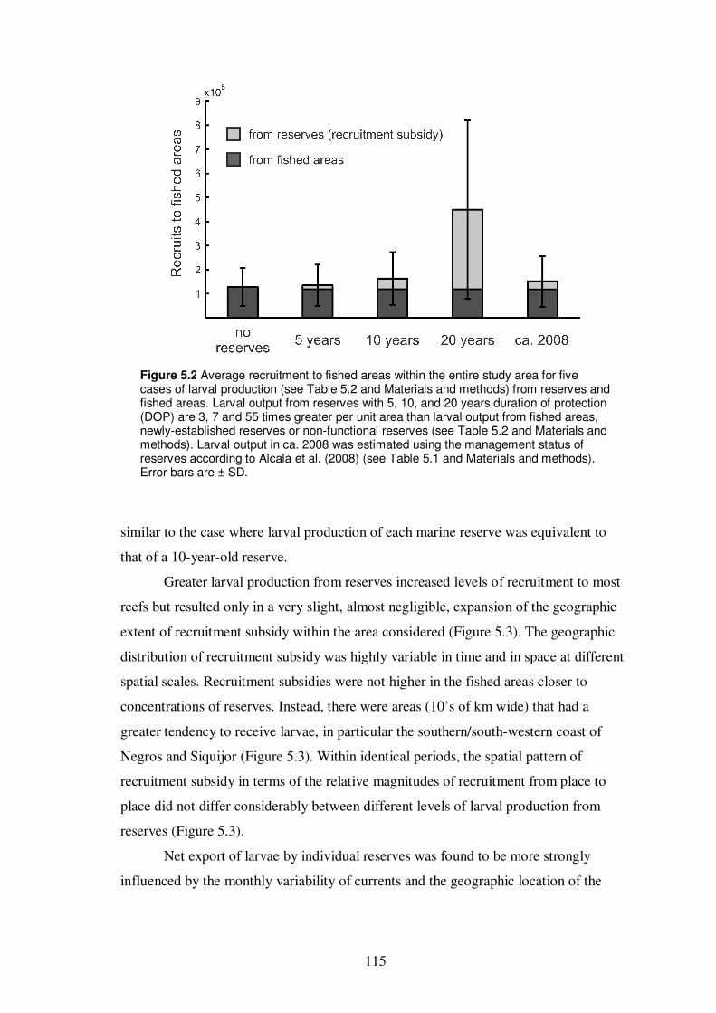
115
similar to the case where larval production of each marine reserve was equivalent to
that of a 10-year-old reserve.
Greater larval production from reserves increased levels of recruitment to most
reefs but resulted only in a very slight, almost negligible, expansion of the geographic
extent of recruitment subsidy within the area considered (Figure 5.3). The geographic
distribution of recruitment subsidy was highly variable in time and in space at different
spatial scales. Recruitment subsidies were not higher in the fished areas closer to
concentrations of reserves. Instead, there were areas (10’s of km wide) that had a
greater tendency to receive larvae, in particular the southern/south-western coast of
Negros and Siquijor (Figure 5.3). Within identical periods, the spatial pattern of
recruitment subsidy in terms of the relative magnitudes of recruitment from place to
place did not differ considerably between different levels of larval production from
reserves (Figure 5.3).
Net export of larvae by individual reserves was found to be more strongly
influenced by the monthly variability of currents and the geographic location of the
Figure 5.2 Average recruitment to fished areas within the entire study area for five cases of larval production (see Table 5.2 and Materials and methods) from reserves and fished areas. Larval output from reserves with 5, 10, and 20 years duration of protection (DOP) are 3, 7 and 55 times greater per unit area than larval output from fished areas, newly-established reserves or non-functional reserves (see Table 5.2 and Materials and methods). Larval output in ca. 2008 was estimated using the management status of reserves according to Alcala et al. (2008) (see Table 5.1 and Materials and methods). Error bars are ± SD.

116
Figure 5.3 Spatial distribution of recruitment subsidy from reserves to fished areas. Results from two cases of larval production (lower – ca. 2008 vs. higher – 20 years duration of protection (DOP); see Table 5.2 and Materials and methods) are shown for contrast. Values plotted are the sum of two months of recruitment (June and September/October) for three years (2006, 2007 and 2008).

117
reserve rather than by larval production inside reserves (Figure 5.4). Most of the 39
reserves were more often net exporters than net importers of larvae, even when larval
production was low (e.g., equivalent to that of a 5-year-old reserve) or equivalent to a
fished area (Figure 5.4). Increasing larval production inevitably resulted in significantly
higher export to import ratios, often up to about 2 orders of magnitude greater.
However, a shift from being a net importer to a net exporter as a consequence of
increased larval production occurred only in some reserves and only in relatively few
instances.
The direction of larval dispersal between reserves was towards the south/south-
west (Figure 5.5), which is consistent with the spatial pattern of recruitment subsidy
(Figure 5.3) and the general current patterns in the study area (Figure 4.2). Probabilities
of self-recruitment within reserves and connectivity between reserves were always very
low regardless of the magnitude of larval production. Probabilities of self-recruitment
were negligible (< 0.0001) or zero for the majority (~70%) of reserves. Probabilities of
connectivity were typically < 0.001. The highest probability for any inter-reserve larval
connection was just 0.03. However, the absolute magnitudes of connectivity between
reserves (i.e., number of successfully recruiting larvae) increased dramatically with
greater larval production (Figure 5.5). The total number of larvae that were exchanged
between reserves increased by 160% (2.6-fold) when larval production was increased
from 3- to 7-fold (5 to 10 year old reserves) and by 660% (7.6-fold) when larval
production was increased from 7- to 55-fold (10 to 20 year old reserves). The increase
in total number of larvae exchanged between reserves, when larval production was
increased from 3- to 55-fold, was 1890% (19.9-fold). The average number of
connections a reserve had with other reserves also increased with greater larval
production (i.e., 47, 57 and 72% of the 31 possible inter-reserve connections at the grid
cell level for the 3-, 7- and 55-fold larval production differentials, respectively) (Figure
5.5).
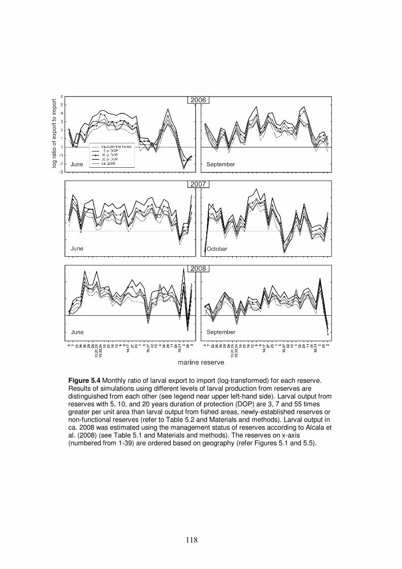
118
Figure 5.4 Monthly ratio of larval export to import (log-transformed) for each reserve. Results of simulations using different levels of larval production from reserves are distinguished from each other (see legend near upper left-hand side). Larval output from reserves with 5, 10, and 20 years duration of protection (DOP) are 3, 7 and 55 times greater per unit area than larval output from fished areas, newly-established reserves or non-functional reserves (refer to Table 5.2 and Materials and methods). Larval output in ca. 2008 was estimated using the management status of reserves according to Alcala et al. (2008) (see Table 5.1 and Materials and methods). The reserves on x-axis (numbered from 1-39) are ordered based on geography (refer Figures 5.1 and 5.5).

119
Figure 5.5 Matrices showing connectivity between reserves when reserves are uniformly protected for 5 years (a), 10 years (b) and 20 years (c). The 39 reserves where larvae were spawned in the larval dispersal model are represented by 32 reef grid cells in the model. Geographic locations are indicated on the x and y axes (refer to Figure 5.1). Self-recruitment to reserves is indicated along the dotted diagonal line. Connectivity in terms of a reserve exporting larvae to other reserves can be examined by reading each matrix from left to right parallel to the x-axis. Connectivity in terms of a reserve receiving larvae from other reserves can be discerned by reading each matrix from bottom to top parallel to the y-axis. Values plotted are the average number of recruits over n = 6 months over 3 years (refer to legend on the leftmost matrix).

120
5.4 Discussion
This study investigated the potential recruitment subsidy from and connectivity
among small community-based reserves in the Philippines. The results showed
considerable potential for such reserves to benefit surrounding reef fisheries at the
predicted spatial scales of ecologically-significant larval connectivity, i.e., within 10’s
of kilometres (Cowen et al. 2006; Jones et al. 2009; Planes et al. 2009; Christie et al.
2010; Saenz-Agudel et al. 2011). However, large recruitment subsidies from these
small reserves are to be expected only after most of them have been continuously and
effectively protected for long periods (i.e., > 10 years), when substantial spawning
biomass has accumulated inside reserves. The model predicted a ~250% (3.5-fold)
increase in total recruitment to fished areas assuming that larval production inside all 39
reserves were to reach a level that is 55 times greater, per unit area, than fished areas
after 20 years of protection. Such a huge larval production differential, and a
considerable period of time to reach it, are likely for large predatory fishes (e.g.,
snappers and groupers) on Philippine reefs given the high rates of fishing mortality on
these reefs, very low fish biomass on intensely fished reefs and the known rates of build
up and attainable levels of biomass inside well-enforced reserves (McManus 1996,
1997; Russ and Alcala 1996, 2003, 2004, 2010; Nañola et al. 2002; Russ et al. 2005;
Nañola et al. 2010).
Recruitment subsidies resulting from less significant larval production
differentials may still benefit highly exploited fisheries. However, these smaller
subsidies will be very difficult to detect in the field because of large temporal and
spatial variations in recruitment (Russ 2002; Halpern et al. 2004; Pelc et al. 2010). For
instance, the model predicted average increases in recruitment to fished areas of only 5
and 21% assuming 3- and 7-fold larval production differentials, respectively. These
increases are much smaller than the CVs of average monthly recruitment, which ranged
from about 60-80%. Of greater significance to present-day conditions, the estimated
increase in recruitment to fished areas given the management status of reserves in ca.
2008 was only 15%. Any recruitment subsidies from reserves were therefore unlikely to
have been noticed by fishers in the past two decades because of natural recruitment
variation.
Field studies on patterns of recruitment in reef fishes (reviewed by Doherty
1991, 2002) provide additional insights on how challenging it would be to detect
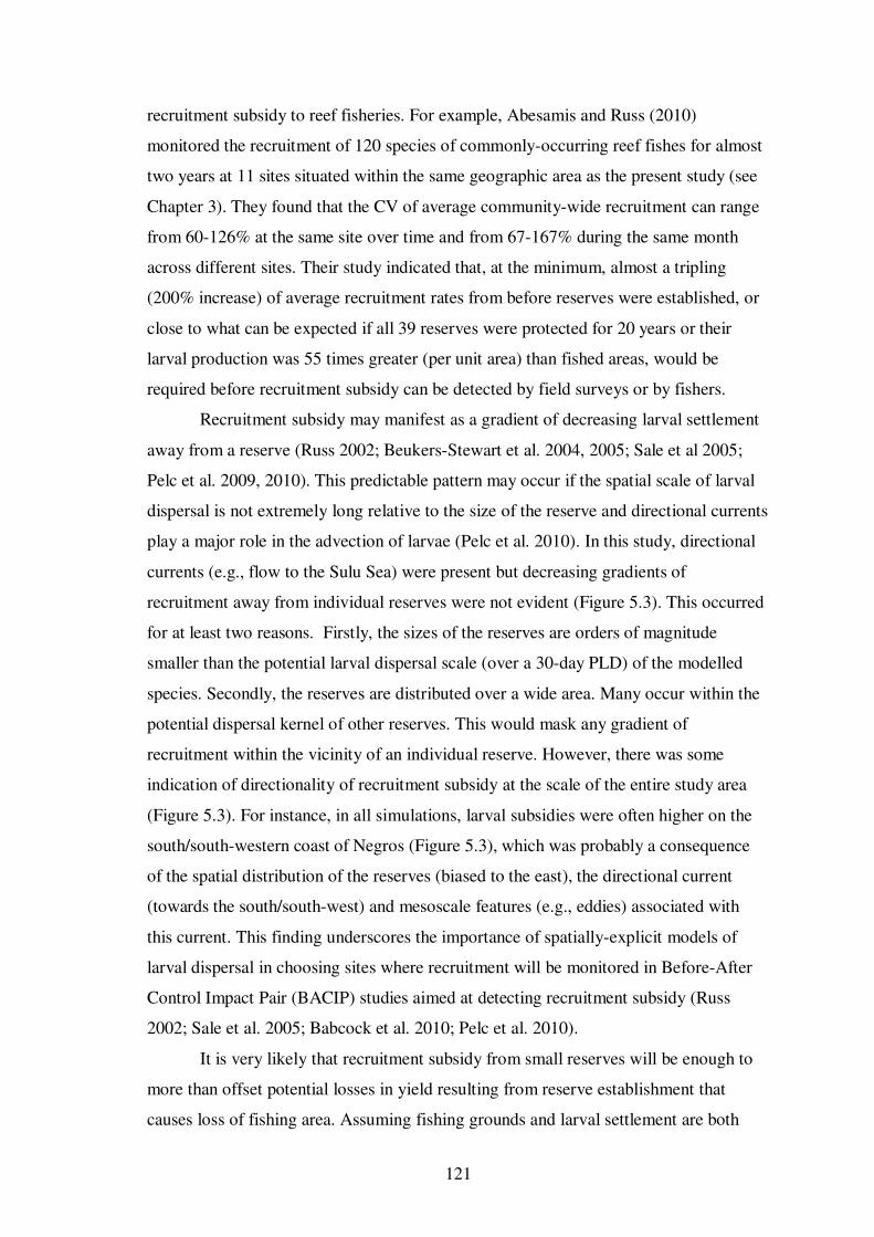
121
recruitment subsidy to reef fisheries. For example, Abesamis and Russ (2010)
monitored the recruitment of 120 species of commonly-occurring reef fishes for almost
two years at 11 sites situated within the same geographic area as the present study (see
Chapter 3). They found that the CV of average community-wide recruitment can range
from 60-126% at the same site over time and from 67-167% during the same month
across different sites. Their study indicated that, at the minimum, almost a tripling
(200% increase) of average recruitment rates from before reserves were established, or
close to what can be expected if all 39 reserves were protected for 20 years or their
larval production was 55 times greater (per unit area) than fished areas, would be
required before recruitment subsidy can be detected by field surveys or by fishers.
Recruitment subsidy may manifest as a gradient of decreasing larval settlement
away from a reserve (Russ 2002; Beukers-Stewart et al. 2004, 2005; Sale et al 2005;
Pelc et al. 2009, 2010). This predictable pattern may occur if the spatial scale of larval
dispersal is not extremely long relative to the size of the reserve and directional currents
play a major role in the advection of larvae (Pelc et al. 2010). In this study, directional
currents (e.g., flow to the Sulu Sea) were present but decreasing gradients of
recruitment away from individual reserves were not evident (Figure 5.3). This occurred
for at least two reasons. Firstly, the sizes of the reserves are orders of magnitude
smaller than the potential larval dispersal scale (over a 30-day PLD) of the modelled
species. Secondly, the reserves are distributed over a wide area. Many occur within the
potential dispersal kernel of other reserves. This would mask any gradient of
recruitment within the vicinity of an individual reserve. However, there was some
indication of directionality of recruitment subsidy at the scale of the entire study area
(Figure 5.3). For instance, in all simulations, larval subsidies were often higher on the
south/south-western coast of Negros (Figure 5.3), which was probably a consequence
of the spatial distribution of the reserves (biased to the east), the directional current
(towards the south/south-west) and mesoscale features (e.g., eddies) associated with
this current. This finding underscores the importance of spatially-explicit models of
larval dispersal in choosing sites where recruitment will be monitored in Before-After
Control Impact Pair (BACIP) studies aimed at detecting recruitment subsidy (Russ
2002; Sale et al. 2005; Babcock et al. 2010; Pelc et al. 2010).
It is very likely that recruitment subsidy from small reserves will be enough to
more than offset potential losses in yield resulting from reserve establishment that
causes loss of fishing area. Assuming fishing grounds and larval settlement are both

122
uniformly distributed, the 6% of total fishing area lost to the 39 reserves would result in
roughly the same loss in recruitment available to fishers, which translates to losses in
future yield. The results suggested that this loss in recruitment can be replaced by a
little more than a 3-fold increase in larval production in reserves (providing > 5% net
gain in recruitment to fished areas), which can happen, for instance, a few years after all
of the reserves have been simultaneously protected for 5 years. Clearly, longer-term
protection (> 5 years) of all the reserves will be necessary to greatly exceed the
compensation for initial losses in recruitment due to reserve protection. Another
potential consequence of reserve establishment is the displacement of fishing effort
(‘fisheries squeeze’) which will increase fishing mortality in fished areas and decrease
catch per fisher. In a spatially-implicit theoretical model, Halpern et al. (2004)
suggested that a 3-fold increase in larval production from reserves is enough to
compensate for displaced fishing effort for up to 50% of fishing area lost to reserves.
Using their approach, the required increase in larval production (or ‘compensation
factor’) for the 6% of fishing area lost to reserves in this study will be just slightly
higher than 2-fold.
Regarding optimal reserve placement, the results suggested that the majority of
the reserves were situated in sites that would allow net export of larvae from reserves
most of the time. Thus, it appears that in this particular case, the ‘haphazard’ or
‘opportunistic’ placement of reserves (see Alcala and Russ 2006) was unlikely to have
been counterproductive in the sense that most reserves are probably not sinks for larvae.
Haphazard placement of reserves will also not be entirely ineffective if some reserves
are situated on good reef habitat, since better habitat will support higher biomass
leading to greater larval production (Crowder et al. 2000). Assessing the effects of
varying habitat quality on recruitment subsidy is beyond the scope of this study but the
available data on the quality of habitat of the reserves in question indicates that most
(~60%) of the reserves include reefs with ‘fair’ to ‘good’ coral cover (i.e., equivalent to
25 to 75% live coral cover) (Table 5.1, Alcala et al. 2008). Nonetheless, the simulations
suggested that potential larval production is not the most critical factor that determines
whether or not reserves will exhibit net export. Instead, local geography and
hydrodynamic patterns are likely to have a stronger influence on where and when net
export is more probable, regardless of the magnitude of larval output. These findings do
not support the view that sources may be created simply by establishing reserves.

123
However, there is no question that the magnitude of larval export from reserves will be
determined by larval production.
The model indicated that self-recruitment within most of the reserves was
highly unlikely, which is not surprising because the spatial scale of larval dispersal was
many times greater than the size of individual reserves. Although finer-scale models
and field studies (e.g., Jones et al. 1999, 2005; Paris and Cowen 2004; Almany et al.
2007; Planes et al. 2009) are required to assess self-recruitment, this result suggested
that the recovery of populations within the small reserves is likely to be greatly
dependent upon recruitment of larvae coming from other populations, especially from
other reserves. A good proportion of the reserves were found to be potentially
connected by demographically-relevant larval exchange, which is consistent with the
expectation of Weeks et al. (2010a) who analysed distances between existing reserves
in the entire Philippines. The probabilities of larval exchange between individual
reserves were very low, but even low numbers of successfully-recruiting larvae
(relative to larval output) are probably important to sustain local populations (Planes et
al. 2009). More significantly, results indicated that any increase in larval production
within individual reserves will directly increase recruitment to other reserves that are
potentially connected to them by larval dispersal, regardless of how small the
probabilities of connectivity are (e.g., Steneck et al. 2009). This indicates that strict
protection of individual reserves that interact via larval exchange will likely lead to
synergistic effects that may increase the rate of recovery of populations within reserves,
and consequently the rate of development of recruitment subsidy.
Substantial recruitment subsidy from networks of reserves will be important to
sustaining fisheries because recruitment is clearly a major determinant of fisheries yield
(e.g., Hjort 1914, 1926; Morgan et al. 1982; Phillips 1986; Caputi et al. 1995; Shanks
and Roegner 2007). Recruitment subsidy becomes all the more important when the
majority of spawning biomass is found inside reserves due to high fishing pressure in
areas open to fishing. Such a ‘scorched earth’ situation was previously noted by Davis
(1977) in lobster populations in Florida and by Pelc et al. (2009) in mussel populations
in South Africa. The present study reflects a similar situation because the abundance of
the hypothetical reef fish stock outside of reserves in the model approximated
overfished levels typical of many Philippine reefs (Russ and Alcala 2002; Russ et al.
2005; Nañola et al. 2002). Recruitment subsidy will most likely be critical to reef
fisheries in many parts of the world since overfishing affects the vast majority of reefs

124
worldwide (mostly in developing countries) (Bryant et al. 1998; Burke et al. 2002;
Burke and Maidens 2004) and reserves are increasingly advocated as viable reef
management tools (Roberts 2000; Russ 2002; Hughes et al. 2003; Sale et al. 2005;
McCook et al. 2010). However, recruitment subsidy cannot sustain fisheries if
management of nursery habitats for settling larvae and juveniles outside of reserves is
neglected (Steneck et al. 2009).
This study is the first to evaluate potential recruitment subsidy to reef fisheries
in the context of existing small, locally-managed reserves situated on heavily fished
coral reefs. The findings emphasise two major factors that will determine whether or
not and when meaningful larval benefits from reserves can be realised. Firstly, strict
protection of existing reserves over the long-term (decades) is essential in order for
reserves to significantly accumulate spawning biomass and increase larval production.
Secondly, reserves must be established in sites with good quality habitat where
protected populations will have a higher chance of attaining high biomass and
exchanging larvae with other reserves. While the latter point implies that knowledge of
source-sink dynamics is required, the establishment of new reserves cannot wait for
perfect data on such dynamics given the first point. Most importantly, the findings of
this study demonstrate the clear potential for networks of no-take marine reserves,
protected effectively over decades, to contribute significantly to food security for
human populations.

125
Chapter 6
General Discussion
6.1. Synthesis – the importance of the monsoons and local geographic setting to
replenishment and connectivity of reef fish populations
A major point that was made at the beginning of this thesis was that we know
very little about the patterns of reproduction, recruitment and population connectivity of
reef fishes in the Coral Triangle compared to other places, such as the Great Barrier
Reef and the Caribbean (Figure 1.2a). Yet, there seems to be tremendous interest to
conserve and manage coral reefs and coral reef fisheries resources in the Coral Triangle
through the use of networks of no-take marine reserves (e.g., Alcala and Russ 2006;
Allen 2008; Clifton 2009; Green et al. 2009; Mills et al. 2010; see Figure 1.2b). A
synthesis of the results of this thesis provides an indication of how the Asian monsoons
and local geographic setting may affect patterns of reef fish population replenishment
and connectivity in the Coral Triangle and how we can assess if existing or future
reserve networks can achieve their conservation and fisheries management goals within
this important region.
It has long been recognised that the annual patterns of reproduction and
recruitment of reef fishes closer to the equator are less seasonal compared to those at
higher latitudes. The results of Chapter 2 and 3 of this thesis confirmed this well-known
pattern. What has received less attention in the past is the potential for the monsoons to
influence the annual patterns of reef fish population replenishment in equatorial
regions, including the Coral Triangle (Johannes 1978; Pauly and Navaluna 1983). The
results of Chapter 2 suggest that the monsoons will probably affect the timing of
reproduction of many species of reef fish differently. Reproduction in different species
may show various responses to more localised changes in the environment caused by
the monsoons, such as degree of wave action depending on exposure to winds,
proximity to localised monsoon-induced upwelling events or regional patterns of
rainfall. For the same species, potential monsoonal effects on reproduction may also
differ geographically because rainfall and wind patterns vary with longitude and
latitude within the Coral Triangle (Wang et al. 2001; Wahl and Morrill 2010).

126
On the other hand, the potential effects of the monsoons on recruitment patterns
seemed more predictable. Chapter 3 and the only other study in the Coral Triangle that
compared reef fish recruitment data against environmental data (i.e., Srinivasan and
Jones 2006) showed that rainfall and wind strength (the latter causing turbulence or
advection at the sea surface) are two monsoonal factors that can negatively affect larval
survival and recruitment of many species. However, the effects of these two factors
probably also vary geographically within the Coral Triangle and between some
taxonomic groups. For instance, as discussed in Chapter 3, heavy rainfall at Kimbe
Bay, Papua New Guinea was detrimental to recruitment of damselfishes but not to
recruitment of wrasses (Srinivasan and Jones 2006). In contrast, lower rainfall levels
did not have a noticeable effect on the recruitment of either damselfishes or wrasses in
the central Philippines (Chapter 3). As for the effects of wind, different wind exposures
in many archipelagic areas of the Coral Triangle may result in temporal patterns of
recruitment that vary between regions at the scale of 100’s of km encompassing many
islands because of different directions of prevailing monsoon winds (e.g., north-
east/south-west in the Philippines; north-west/south-east in Papua New Guinea and
Indonesia). Variable temporal patterns of recruitment may also occur at more limited
spatial scales within these regions, such as amongst smaller islands and locations within
larger islands.
It is still difficult to predict the annual patterns of population replenishment of
various species of reef fishes at different places within the Coral Triangle. What has
become clearer in this thesis is that the degree of monsoonal effects at a particular place
can influence the timing and shape of replenishment peaks within the year. Several
characteristic annual patterns of reef fish replenishment may be present within the Coral
Triangle. These characteristic annual patterns of replenishment may also dictate the
strength of density-dependent post-settlement processes (e.g., competition, predation
and mortality) at different times of the year, potentially affecting the structure of local
reef fish populations. The importance of the monsoons in influencing patterns of
replenishment in reef fishes can be further tested by comparing sites that differ in their
exposures to monsoon winds or have different rainfall patterns. With regards to the
potential effects of wind stress on larval survival, data from sites that are not exposed to
monsoon winds (e.g., bays that are surrounded by high mountains) may provide
valuable insights.

127
Patterns of dispersal of reef fish larvae in the Coral Triangle may also vary
considerably according to the monsoons, depending on how winds affect ocean
circulation patterns (reviewed by Cowen 2002). For instance, McManus (1994) showed
that potential large-scale (100’s of km) trajectories of larval transport from spawning
populations on reefs in the South China Sea (Spratly Islands) can vary significantly
within a year because the monsoons have a strong influence on the surface current
patterns of that region. However, dramatic changes in potential patterns of larval
connectivity between local populations caused by the monsoons were not so evident in
Chapter 4 because of the hydrodynamic characteristics of the Bohol Sea, particularly
the persistent unidirectional (westward) current that passes within the vicinity of the
sites that were studied. Nonetheless, potential patterns of larval connectivity between
other local populations also situated within the Bohol Sea may be influenced strongly
by mesoscale (10’s of km), monsoon-induced, changes in surface current patterns
(Ablan 2005, 2006). These preceding examples, that suggest different patterns of larval
dispersal between two areas (South China Sea vs. Bohol Sea) and within the same area
(Bohol Sea), emphasise how the local oceanographic setting can greatly influence
potential patterns of larval connectivity. The development of high-resolution (< 10 km)
models of monthly sea surface circulation patterns at the relevant spatial scales (10’s to
100’s of km) and the validation of these models with empirical data (e.g.,
oceanographic surveys, drifter tracking data, etc.) should therefore be given some
priority. Such models probably do not yet exist for many parts of the Coral Triangle.
On the other hand, there are no studies available to date that demonstrate any
relationship between monsoon winds and smaller-scale (within 10’s of km) circulation
patterns that may promote retention of reef fish larvae near their natal populations.
Present evidence suggests that wind is probably more important for transport
mechanisms that promote successful settlement of late-stage larvae and not necessarily
for retention mechanisms that may be crucial during earlier stages of larval
development (Cowen 2002). Some of the important physical mechanisms that could
promote larval retention occur 10’s of m below the surface (e.g., onshore flow), which
swimming larvae can take advantage of through vertical migration in order to avoid
offshore flow due to prevailing winds (Cowen et al. 2000; Paris and Cowen 2004).
Finally, the approach that was taken in Chapter 5 provides an indication of what
may be required to determine if new or existing reserve networks have the potential to
achieve their conservation and fisheries management objectives for targeted reef fish

128
species in some of the most heavily exploited regions of the Coral Triangle. Firstly,
models of reef fish larval dispersal that incorporate the best data available on local
oceanographic patterns and larval biology (swimming and sensory behaviour, larval
mortality) must be developed. Secondly, these models should take into account any
major variations in current patterns caused by the monsoons. Thirdly, estimates of the
present population density, biomass and size structure of the target species inside
reserves, or proposed reserves, and outside reserves must be obtained through field
surveys. Fourthly, models of population recovery of the targeted species in response to
reserve protection must be coupled to the larval dispersal model. These models of
population recovery can be based on time-series data obtained from one reserve over
the long-term (decades) with the appropriate control sites (fished areas) (e.g., Russ and
Alcala 2010). Alternatively, these models can be based on comparisons of many
reserves that have habitats that are as similar as possible but with different durations of
protection (spanning decades) against appropriate control sites (McClanahan and
Graham 2005; Russ et al. 2005; McClanahan et al. 2007; Stockwell et al. 2009). Fifthly,
basic information on the life histories of the targeted species must be obtained in the
field and incorporated into the larval dispersal and population recovery models. This
includes size and age at sexual maturity inside and outside reserves (e.g., Taylor and
McIlwain 2010), body size and batch fecundity relationships, spawning frequency and
spawning output per unit area, the best temporal ‘windows’ for spawning and
recruitment which are likely to be related to the monsoons (Chapter 2 and 3), spatial
patterns of spawning (if the species undergoes spawning migrations) and distribution of
settlement habitats for larvae or nursery habitats for juveniles. The collection of basic
life history data on key groups of targeted reef fish species (groupers, snappers,
emperors, parrotfishes and surgeonfishes) is extremely important and should be given a
high priority. For instance, a major limitation of the model that was used in Chapter 5 is
the lack of detailed information on the spatial distribution of critical settlement and
juvenile habitats for the model species (i.e., snappers, which may use non-reef
settlement or nursery habitats). Better information on the distribution of these habitats
will probably affect the conclusions about the spatial patterns of recruitment subsidy
and inter-reserve connectivity to some extent.

129
6.2 Climate change and the influence of the monsoons on reef fish population
dynamics
The preceding section discussed the potential of the monsoons to profoundly
affect the patterns of replenishment and population connectivity of reef fishes in the
Coral Triangle. The variability of the Asian monsoons is somehow linked to the El
Niño-Southern Oscillation (ENSO) (Webster 1995; Hu et al. 2000; Cook et al. 2010).
Models of climate change also suggest that the frequency of warm ENSO events (El
Niño), which are sometimes followed by cold ENSO events (La Niña), is expected to
increase for many years into the future if ‘greenhouse’ gas concentrations in the
atmosphere continue to increase (e.g., Trenberth and Hoar 1997; Timmerman et al.
1999; Hu et al. 2000). Thus, how climate change may affect the dynamics of reef fish
populations in the Coral Triangle is of considerable significance. Although the dynamic
processes that govern the spatial and temporal variability of the Asian monsoons and
their complex relationships with the ENSO are still not well-understood (Webster and
Palmer 1997; Wu and Chan 2005; Wahl and Morrill 2010), some possible
consequences of climate change for the monsoons and, in turn, the dynamics of reef
fish populations are worth exploring.
Weaker summer monsoon winds in some areas of the Coral Triangle (e.g.,
south-west monsoon in the Philippines) are associated with El Niño decaying years
(Chou et al. 2003). El Niño is also usually characterised by decreased rainfall levels in
the western Pacific, including the Coral Triangle (e.g., Philippines and Indonesia),
leading to severe drought (Webster and Palmer 1997). Weaker winds may be
favourable to the survival of larvae in the pelagic environment (Chapter 3) while
decreased rainfall probably has no effect on larval survival or recruitment (Srinivasan
and Jones 2006). Thus, higher levels of recruitment may be expected for many species
during El Niño decaying years. However, weaker winds and higher sea surface
temperatures associated with the El Niño usually result in widespread coral bleaching in
many areas of the Coral Triangle (Brown and Suharsono 1990; Arceo et al. 2001;
Raymundo and Maypa 2002; Jones et al. 2004). Mass mortality of corals due to
bleaching may work against potential gains in recruitment for species that are
dependent on live corals as habitat for new settlers and juveniles (Booth and Berretta
2002; Bonin et al. 2009). Moreover, the loss of live coral habitats can impair the
recruitment of many reef fish species over many years (e.g., Jones et al. 2004; Garpe et

130
al. 2006; Wilson et al. 2006; Graham et al. 2007). On the other hand, the La Niña is
usually characterised by higher annual rates of rainfall in the western Pacific, including
the Coral Triangle region (Webster and Palmer 1997). In places where rainfall becomes
exceptionally heavy during the La Niña, the recruitment of some species (e.g.,
damselfishes) could be negatively affected (Srinivasan and Jones 2006).
Any alterations of ocean circulation patterns as a result of climate change may
also have direct consequences for patterns of larval dispersal and connectivity between
local populations of reef fishes. As mentioned above, the summer monsoon winds in
some areas of the Coral Triangle may weaken during the El Niño, potentially altering
large-scale hydrodynamic patterns and thus the patterns of reef fish population
connectivity. With regards to how climate change can influence other oceanographic
processes that may be important to reef fish reproduction and larval survival, at least
one study within the Coral Triangle has shown that increased precipitation during the
La Niña can suppress monsoon-driven upwelling in a coastal area (Villanoy et al.
2011). Failure of upwelling events in the vicinity of reefs may have implications for
reproduction of reef fishes that are ‘cuing-in’ to upwelling signals (McIlwain et al.
2006) or to the survival of reef fish larvae at first-feeding.
No studies to date have examined how potential relationships between the
monsoons and the ENSO may influence patterns of reef fish replenishment or
connectivity. In fact, recent reviews of the potential effects of climate change on
individual performance, population or community dynamics of reef fishes (e.g., Wilson
et al. 2006; Munday et al. 2008) had little to say about the possible consequences of
alterations in environmental factors that characterise the monsoons (i.e., wind and
rainfall). The effects of climate change on the monsoons and their potential
implications for the dynamics and management of reef fish populations in the Coral
Triangle should be given more attention in future studies.
6.3 Reserve network goals and the future of ad hoc reserve networks in the
Philippines
The results of Chapter 5 suggest that even no-take reserves that were established
with very little consideration of optimum size, spacing and placement can still provide
some of the most important larval benefits that are expected from marine reserve
networks. The Philippine reserves that were studied clearly had the potential to

131
significantly subsidise recruitment to fished areas within their vicinity (within 10’s of
km) and to interact with each other through larval exchange. This is an important
positive message because the ad hoc establishment of hundreds of small marine
reserves in that country has evidently fallen short of achieving conservation targets,
such as sufficient reserve coverage of critical habitats and biodiversity representation
(Weeks et al. 2010a). The establishment of larger reserves that protect more substantial
areas of critical marine habitats and the consideration of larval connectivity between
these reserves should still be strongly encouraged (Weeks et al. 2010a, b). Furthermore,
if systematic conservation planning is undertaken to design new or improve existing
reserve networks, then incorporating reliable information on patterns of larval
connectivity for a range of important species should be given priority. However, the
results of Chapter 5 indicate that the effective and continuous protection of reserves
from any form of extractive or destructive activity is the most crucial factor that will
determine the success of reserve networks. No reserve network will be effective
without the long-term support from local stakeholders. If considerable fisheries
enhancement is the main expectation from protecting reserves, then local stakeholders
must be convinced that reserves will eventually provide substantial recruitment
benefits. Also note that some local spillover and tourism benefits from reserves may
also help convince stakeholders to continue reserve protection indefinitely (e.g.
Abesamis et al 2006a, Alcala and Russ 2006). Most importantly, local stakeholders also
must eventually ‘feel’ these benefits.
There are at least two potential ways in which scientists can help convince local
stakeholders to protect reserves over the long-term. First is to plan and assist in the
implementation of a before-after-control-impact (BACIP) type experiment (Russ 2002;
Sale et al. 2005; Babcock et al. 2010; Pelc et al. 2010) to test recruitment subsidy from
reserves. This must involve the participation of local fishing communities. Predictions
on the locations of ‘control’ sites (reefs that are not likely to receive larval subsidies
from reserves) and ‘impact’ sites (reefs that are likely to receive larval subsidies from
reserves) can come from more sophisticated models of population recovery of the
chosen target species inside reserves, potential larval output from reserves and fished
populations, and spatial and temporal estimates of larval connectivity (discussed in
Section 6.1). Measurements of recruitment subsidy can be done through monitoring of
catch-per-unit effort of fishers at control and impact sites that are open to fishing
(standardised across sites according to fisher population) and visual surveys of

132
recruitment at the appropriate habitats within the same sites, as well as inside reserves
that are ‘impacted’ by larval subsidies. Note that the choice of target reef fish species
will be critical to this experiment. The most appropriate species for the experiment are
probably those that: 1) are highly important to local fisheries; 2) are relatively short-
lived and fast-growing; 3) have relatively fast rates of population recovery in response
to reserve protection; and 4) have recruits that are relatively easy to monitor. Species
that are very important to local fisheries and are quicker to develop net larval export
from reserves may help convince local stakeholders within shorter periods. In the
context of reef fisheries and recovery of target species inside reserves in the
Philippines, parrotfishes (Scaridae) are probably some of the best species to use for
such an experiment (Stockwell et al. 2009; Chapter 3 and Abesamis and Russ 2010).
The second manner by which scientists can help convince local stakeholders to
support the long-term protection of reserves is by empirically validating the presence of
larval connections from reserves to fished areas and from reserves to other reserves.
Larval connectivity between two places can be convincingly demonstrated through
parentage analysis using multiple microsatellite DNA markers, which can be done in
combination with larval mark-recapture experiments via chemical tagging of larval
otoliths (e.g., Jones et al. 2005; Almany et al. 2007; Planes et al. 2009; Williamson et
al. 2009; Christie et al. 2010; Saenz-Agudelo et al. 2011). For instance, validation
experiments can be performed between sites that are suspected to be strongly connected
by larval dispersal based on the findings of Chapter 4 and 5. Validation studies can also
be designed to complement the BACIP fisheries experiment described above. Needless
to say, it is crucial that the basic principles behind sophisticated methods of predicting
and validating reef fish larval connectivity are explained to local stakeholders using
concepts that they can easily grasp. The same undoubtedly applies to the results of the
BACIP and validation studies. Stakeholders who are sufficiently informed about how
their reef fishery resources function can mean the difference between failure and
success of reserve networks.

133
Bibliography
Abesamis RA, Russ GR (2005) Density-dependent spillover from a marine reserve:
long-term evidence. Ecological Applications 15:1798-1812
Abesamis RA, Russ GR (2010) Patterns of recruitment of coral reef fishes in a
monsoonal environment. Coral Reefs 29:911-921
Abesamis RA, Alcala AC, Russ GR (2006a) How much does the fishery at Apo Island
benefit from spillover of adult fish from the adjacent marine reserve? Fishery
Bulletin 104:360-375
Abesamis RA, Russ GR and Alcala AC (2006b) Gradients of abundance of fish across
no-take marine reserve boundaries: evidence from Philippine coral reefs.
Aquatic Conservation: Marine and Freshwater Ecosystems 16:349-371
Ablan, MC (2005) Assessing the utility of microsatellite markers for the identification
of stock boundaries and estimation of exchanges among populations of
Dascyllus trimaculatus and Pterocaesio pisang in the Bohol Sea, Central
Philippines. PhD Thesis. University of the Philippines, Diliman Quezon City
207 p.
Ablan, MC (2006) Genetics and the study of fisheries connectivity in Asian developing
countries. Fisheries Research 78:158-168
Agardy T, Notarbartolo di Sciara G, Christie P (2011) Mind the gap: addressing the
shortcomings of marine protected areas through large scale marine spatial
planning. Marine Policy 35:226-232
Alcala AC (1981) Fish yields of coral reefs of Sumilon Island, central Philippines.
Natural Resources Council of the Philippines, Research Bulletin 36:1-7

134
Alcala AC (1988) Effects of marine reserves on coral fish abundances and yields of
Philippine coral reefs. Ambio 17:194-199
Alcala AC (1998) Community-based coastal resource management in the Philippines: a
case study. Ocean and Coastal Management 38:179-186
Alcala AC (2001) Marine Reserves in the Philippines: Historical Development, Effects
and Influence on Marine Conservation Policy. Bookmark Inc., Manila,
Philippines
Alcala AC, Luchavez TF (1981) Fish yield of the coral reef surrounding Apo Island,
central Visayas, Philippines. Proceedings of the 4th International Coral Reef
Symposium 1:69-73
Alcala AC, Russ GR (1990) A direct test of the effects of protective management on
abundance and yield of tropical marine resources. Journal Conseil International
pour l'Exploration de la Mer 47:40-47
Alcala AC, Russ GR (2002) Status of Philippine coral reef fisheries. Asian Fisheries
Science 15:177-192
Alcala AC, Russ GR (2006) No-take marine reserves and reef fisheries management in
the Philippines: a new People Power revolution. Ambio 35:245-254
Alcala AC, Russ GR, Maypa AP, Calumpong HP (2005) A long-term, spatially
replicated experimental test of the effect of marine reserves on local fish yields.
Canadian Journal of Fisheries and Aquatic Sciences 62: 98-108
Alcala AC, Bucol AA, Nillos-Kleiven P (2008) Directory of Marine Reserves in the
Visayas, Philippines. Foundation for the Philippine Environment and Silliman
University-Angelo King Center for Research and Environmental Management
(SUAKCREM), Dumaguete City, Philippines. 178 p.

135
Aliño PM, Palomar NE, Arceo HO, Uychiaoco AT (2002) Challenges and opportunities
for marine protected area (MPA) management in the Philippines. Proceedings of
the 9th International Coral Reef Symposium, Ministry of Environment,
Indonesian Institute of Sciences, and the International Society for Reef Studies
2: 635–640 (available at http://www.coremap.or.id/ downloads/ICRS9th-
Alino.pdf)
Aliño, PM, Miclat RI, Gonzales R, Arceo HO (2007) Marine Protected Area Support
Network: sustaining mechanism for MPA management. Paper presented at the
2nd National ICZM Congress: Coastal Zone Philippines 2, 27-29 October 2007,
Iloilo City, Philippines
Allen GR (2008) Conservation hotspots of biodiversity and endemism for Indo-Pacific
coral reef fishes. Aquatic Conservation: Marine and Freshwater Ecosystems
18:541–556
Allen G, Steene R, Humann P, DeLoach N (2003) Reef Fish Identification - Tropical
Pacific. New World Publications, Inc. Jacksonville, Florida, USA. 475 p.
Allison GW, Lubchenco J, Carr MH (1998) Marine reserves are necessary but not
sufficient for marine conservation. Ecological Applications 8:S79–S92
Almany GR, Berumen ML, Thorrold SR, Planes S, Jones GP (2007) Local
replenishment of coral reef fish populations in a marine reserve. Science
316:742-744
Almany GR, Connolly SR, Heath DD, Hogan JD, Jones GP, McCook LJ, Mills M,
Pressey RL, Williamson DH (2009) Connectivity, biodiversity conservation and
the design of marine reserve networks for coral reefs. Coral Reefs 28:339-351
Anand PEV, Pillai NGK (2002) Reproductive biology of some common coral reef
fishes of the Indian EEZ. Journal of the Marine Biological Association of India
44:122-135
136
Anand PEV, Pillai NGK (2005) Occurrence of juvenile fishes on the seagrass beds of
Kavaratti Atoll, Lakshadweep, India. Indian Journal of Fisheries 52:459-467
Anderson JT (1988) A review of size dependent survival during pre-recruit stages of
fishes in relation to recruitment. Journal of Northwest Atlantic Fishery Science
8:55-66
Aragones NV (1987) Taxonomy, distribution, and relative abundance of juvenile
siganids and aspects of the padas fishery in Bolinao, Pangasinan. MSc thesis,
University of the Philippines, 66 p.
Arceo HO (2004) Patterns and role of recruitment on the community dynamics of reef
fishes in the Philippines. MSc thesis, University of the Philippines, 138 p.
Arceo HO, Quibilan MC, Aliño PM, Lim G, Licuanan WY (2001) Coral bleaching in
the Philippines: coincident evidences with mesoscale thermal anomalies.
Bulletin of Marine Science 69:579-593
Arceo HO, Alino PM, Gonzales ROM (2008) Where are we now with marine protected
areas? In: Alino PM, Geronimo RC (eds) Reefs through time 2008: Initiating
the State of the Coasts Reports. Coral Reef Information Network of the
Philippines (Philreefs), MPA Support Network, Marine Environment &
Resources Foundation Inc., and the Marine Science Institute, University of the
Philippines, 152 p.
Armsworth PR (2002) Recruitment limitation, population regulation, and larval
connectivity in reef fish metapopulations. Ecology 83:1092-1104
Babcock RC, Shears NT, Alcala AC, Barrett NS, Edgar GJ, Lafferty KD, McClanahan
TR, Russ GR (2010) Decadal trends in marine reserves reveal differential rates
of change in direct and indirect effects. Proceedings of the National Academy of
Sciences 107:18256-18261
137
Bailey KM, Macklin SA (1994) Analysis of patterns in larval walleye pollock Theragra
chalcogramma survival and wind mixing events in Shelikof Strait, Gulf of
Alaska. Marine Ecology Progress Series 113:1-12
Bakun A, Beyer J, Pauly D, Pope JG, Sharp GD (1982) Oceanic sciences in relation to
living resources. Canadian Journal of Fisheries and Aquatic Sciences 39:1059-
1070
Bellwood DR (1988) Seasonal changes in the size and composition of the fish yield
from reefs around Apo Island, central Philippines, with notes on methods of
yield estimation. Journal of Fish Biology 32:881-893
Bellwood DR, Hughes TP, Folke C, Nystrom 2004. Confronting the coral reef crisis.
Nature 429:827-833
Bergenius MAJ, Meekan MG, Robertson DR, McCormick MI (2002) Larval growth
predicts the recruitment success of a coral reef fish. Oecologia 131:521–525
Bergenius MAJ, McCormick MI, Meekan MG, Robertson D (2005) Environmental
influences on larval duration, growth and magnitude of settlement of a coral reef
fish. Marine Biology 147:291-300
Beukers-Stewart BD, Vause BJ, Mosley MWJ, Brand AR (2004) Evidence for larval
export of scallops from a small closed area off the Isle of Man. ICES Annual
Conference, September 2004, Vigo, Spain
Beukers-Stewart BD, Vause BJ, Mosley MWJ, Rossetti HL, Brand AR (2005) Benefits
of closed area protection for a population of scallops. Marine Ecology Progress
Series 298:189-204
Bode M, Bode L, Armsworth PR (2006) Larval dispersal reveals regional sources and
sinks in the Great Barrier Reef. Marine Ecology Progress Series 308:17-25

138
Boersma PD, Parrish JK (1999) Limiting abuse: marine protected areas, a limited
solution. Ecological Economics 31:287-304
Bohnsack JA, Ault JS (1996) Management strategies to conserve marine biodiversity.
Oceanography 9:73-82
Bonin MC, Munday PL, McCormick MI, Srinivasan M, Jones GP (2009) Coral-
dwelling fishes resistant to bleaching but not to mortality of host corals. Marine
Ecology Progress Series 394: 215-222
Booth DA, Berretta GA (2002) Changes in a fish assemblage after a coral bleaching
event. Marine Ecology Progress Series 245:205-212
Botsford L, Hastings A, Gaines S (2001) Dependence of sustainability on the
configuration of marine reserves and larval dispersal distance. Ecology Letters
4:144-150
Botsford LW, White JW Coffroth MA, Paris CB, Planes S, Shearer TL, Thorrold SR,
Jones GP (2009) Connectivity and resilience of coral reef metapopulations in
marine protected areas: matching empirical efforts to predictive needs. Coral
Reefs 28:327-337
Brown BE, Suharsono (1990) Damage and recovery of coral reefs affected by El Niño
related seawater warming in the Thousand Islands, Indonesia. Coral Reefs
8:163-170
Bryant D, Burke L, McManus J, Spalding M (1998) Reefs at Risk – A Map-Based
Indicator of Threats to the World’s Coral Reefs. World Resources Institute, 56
p.
Burke L, Maidens J (2004) Reefs at Risk in the Caribbean. World Resources Institute,
80 p.

139
Burke L, Selig E, Spalding M (2002) Reefs at Risk in Southeast Asia. World Resources
Institute, 76 p.
Cabaitan PC, Gomez ED, Aliño PM (2008) Effects of coral transplantation and giant
clam restocking on the structure of fish communities on degraded patch reefs.
Journal of Experimental Marine Biology and Ecology 357:85-98
Cabanban AS (1984) Some aspects of the biology of Pterocaesio pisang in the Central
Visayas. MSc thesis, University of the Philippines, 69 p.
Cabrera OC, Villanoy CL, David LT, Gordon AL (2011) Barrier layer control of
entrainment and upwelling in the Bohol Sea, Philippines. Oceanography
24:130-141
Caley MJ, Carr MH, Hixon MA, Hughes TP, Jones GP, Menge BA (1996) Recruitment
and the local dynamics of open marine populations. Annual Review of Ecology
and Systematics 27:477-500
Campos WL, Aliño PM (2008) Recent advances in the management of marine
protected areas in the Philippines. Kuroshio Science 2:29-34
(http://hdl.handle.net/10126/3159)
Caputi N, Brown RS, Chubb CF (1995) Regional prediction of the western rock lobster,
Panulirus cygnus, commercial catch in Western Australia. Crustaceana 68:245-
256
Carpenter KE (1988) FAO Species Catalogue. Vol. 8 Fusiliers fishes of the world. An
annotated and illustrated catalogue of Caesionid species known to date. FAO
Fisheries Synopsis 125, 75 p.
Carpenter KE, Alcala AC (1977) Philippine coral reef fisheries resources. Part II.
Muro-ami and kayakas reef fisheries, benefit or bane? Philippine Journal of
Fisheries 15:217-235

140
Carpenter KE, Springer VG (2005) The center of the center of marine shore fish
biodiversity: the Philippine Islands. Environmental Biology of Fishes 72:467-
480
Carpenter KE, Miclat R, Albaladejo VD, and Corpuz VT (1981) The influence of
substrate structure on the local abundance and diversity of Philippine reef fishes.
Proceedings of the 4th International Coral Reef Symposium 2:497-502
Carpenter KE, Barber PH, Crandall ED, Ablan-Lagman MCA, Ambariyanto,
Mahardika GN, Manjaji-Matsumoto BM, Juinio-Meñez MA, Santos MD,
Starger CJ, Toha AH (2011) Comparative phylogeography of the Coral Triangle
and implications for marine management. Journal of Marine Biology
doi:10.1155/2011/396982
Carpenter KE, Abrar M, Aeby G, Aronson RB, Banks S, Bruckner A, Chiriboga A,
Cortés J, Delbeek JC, DeVantier L, Edgar GJ, Edwards AJ, Fenner D, Guzmán
HM, Hoeksema BW, Hodgson G, Johan O, Licuanan WY, Livingstone SR,
Lovell ER, Moore JA, Obura DA, Ochavillo D, Polidoro BA, Precht WF,
Quibilan MC, Reboton C, Richards ZT, Rogers AD, Sanciangco J, Sheppard A,
Sheppard C, Smith J, Stuart S, Turak E, Veron JEN, Wallace C, Weil E, Wood
E (2008) One-third of reef-building corals face elevated extinction risk from
climate change and local impacts. Science 321:560-563
Carr MH, Reed DC (1993) Conceptual issues relevant to marine harvest refuges:
examples from temperate fishes. Canadian Journal of Fisheries and Aquatic
Sciences 50:2019-2028
Choi C, Takemura A, Takano K (1996) Ovarian development and changes in serum
vitellogenin during the annual reproductive cycle of the female fusilier, Caesio
diagramma. Galaxea 13:35-45
Chou C, Tu J-Y, Yu J-Y (2003) Interannual variability of the Western North Pacific
summer monsoon: differences between ENSO and non-ENSO years. Journal of
Climate 16:2275-2287
141
Christie MR, Tissot BN, Albins MA, Beets JP, Jia Y, Ortiz DM, Thompson SE, Hixon
MA (2010) Larval connectivity in an effective network of marine protected
areas. PLoS ONE 5(12): e15715. doi:10.1371/journal.pone.0015715
Clarke KR, Ainsworth M (1993) A method of linking multivariate community structure
to environmental variables. Marine Ecology Progress Series 92:205-219
Clarke KR, Warwick RM (2001) Change in marine communities: an approach to
statistical analysis and interpretation. 2nd
edition Primer-E, Plymouth
Clifton J (2009) Science, funding and participation: key issues for marine protected
area networks and the Coral Triangle Initiative. Environmental Conservation
36:91
Clifton KE (1995) Asynchronous food availability on neighboring Caribbean coral
reefs determines seasonal patterns of growth and reproduction for the
herbivorous parrotfish Scarus iserti. Marine Ecology Progress Series 116:39-46
Cook ER, Anchukaitis KJ, Buckley BM, D’Arrigo RD, Jacoby GC, Wright WE (2010)
Asian monsoon failure and megadrought during the last millennium. Science
328:486-489
Cowen RK (2002) Larval dispersal and retention and consequences for population
connectivity. In: Sale PF (ed) Coral Reef Fishes: Dynamics and Diversity in a
Complex Ecosystem. Academic Press p. 149-170
Cowen RK, Paris CB, Srinivasan A (2006) Scaling of connectivity in marine
populations. Science 311:522-527
Cowen RK, Gawarkiewicz G, Pineda J, Thorrold SR, Werner FE (2007) Population
connectivity in marine systems: an overview. Oceanography 20:14-21

142
Cowen RK, Lwiza KMM, Sponaugle S, Paris CB, Olson DB (2000) Connectivity of
marine populations: open or closed? Science 287:857-859
Crowder LB, Lyman SJ, Figueira WF, Priddy J (2000) Source-sink population
dynamics and the problem of siting marine reserves. Bulletin of Marine Science
66:799-820
Cudney-Bueno R, Lavin MF, Marinone SG, Raimondi PT, Shaw WW (2009) Rapid
effects of marine reserves via larval dispersal. PLoS ONE 4(1): e4140.
doi:10.1371/journal.pone.0004140
Cushing DH (1982) Climate and Fisheries. Academic Press, New York. 373 p.
Cushing DH (1987) Population biology and the management of fisheries. Trends in
Ecology and Evolution 2:138-139
Davis GE (1977) Fishery harvest in an underwater park. Proceedings of the 3rd
International Coral Reef Symposium 2:605-608
Doherty PJ (1981) Coral reef fishes: recruitment-limited assemblages? Proceedings of
the 4th International Coral Reef Symposium 4:465-470
Doherty PJ (1991) Spatial and temporal patterns in recruitment. In: Sale PF (ed) The
Ecology of Fishes on Coral Reefs. Academic Press, San Diego, p. 261-293
Doherty PJ (2002) Variable replenishment and the dynamics of reef fish populations.
In: Sale PF (ed) Coral Reef Fishes: Dynamics and Diversity in a Complex
Ecosystem. Academic Press, p. 327-355
Doherty PJ, Fowler AJ (1994) An empirical test of recruitment limitation in a coral-reef
fish. Science 263:935–939
Doherty PJ, Williams DM (1988) The replenishment of coral reef fish populations.
Oceanography and Marine Biology: an Annual Review 26:487-551

143
Dugan JE, Davis GE (1993) Applications of marine refugia to coastal fisheries
management. Canadian Journal of Fisheries and Aquatic Sciences 50:2029-2042
Dupont L, Ellien C, Viard F (2007) Limits to gene flow in the slipper limpet Crepidula
fornicata as revealed by microsatellite data and a larval dispersal model. Marine
Ecology Progress Series 349:125-138
Emata AC (2003) Reproductive performance in induced and spontaneous spawning of
the mangrove red snapper, Lutjanus argentimaculatus: a potential candidate
species for sustainable aquaculture. Aquaculture Research 34:849-857
Evans RD, Russ GR, Kritzer JP (2008) Batch fecundity of Lutjanus carponotatus
(Lutjanidae) and implications of no-take marine reserves on the Great Barrier
Reef, Australia. Coral Reefs 27:179-189
Fisher R, Bellwood DR, Job SD (2000) Development of swimming abilities in reef fish
larvae. Marine Ecology Progress Series 202:163-173
Friedlander AM, Brown EK, Jokiel PL, Smith WR, Rodgers KS (2003) Effects of
habitat, wave exposure, and marine protected area status on coral reef fish
assemblages in the Hawaiian archipelago. Coral Reefs 22:291-305
Gaines S, Gaylord B, Largier JL (2003) Avoiding current oversights in marine reserve
design. Ecological Applications 13:S32-46
Gallego A, Heath MR, McKenzie E, Cargill LH (1996) Environmentally induced short-
term variability in the growth rates of larval herring. Marine Ecology Progress
Series 137:11-23
Ganias K, Somarakis S, Machias A, Theodorou A (2004) Pattern of oocyte
development and batch fecundity in the Mediterranean sardine. Fisheries
Research 67:13-23

144
Garpe KC, Yahya SAS, Lindahl U, Ohman MC (2006) Long-term effects of the 1998
coral bleaching event on reef fish assemblages. Marine Ecology Progress Series
315:237-247
Gell FR, Roberts CM (2003) Benefits beyond boundaries: the fishery effects of marine
reserves. Trends in Ecology and Evolution 18:448-455
Gerlach G, Atema J, Kingsford MJ, Black KP, Miller-Sims V (2007) Smelling home
can prevent dispersal of reef fish larvae. Proceedings of the National Academy
of Sciences 104:858-863
Graham NAJ, Wilson SK, Jennings S, Polunin NVC, Robinson J, Bijoux JP, Daw TM
(2007) Lag effects in the impacts of mass coral bleaching on coral reef fish,
fisheries, and ecosystems. Conservation Biology 21:1291-1300
Grahame J (1976) Zooplankton of a tropical harbour: the numbers, composition and
response to physical factors of zooplankton in Kingston Harbour, Jamaica.
Journal of Experimental Marine Biology and Ecology 25:219-237
Green AL, Smith SE, Lipsett-Moore G, Groves C, Peterson N, Sheppard S, Lokani P,
Hamilton R, Almany J, Aitsi J, Bualia L (2009) Designing a resilient network of
marine protected areas for Kimbe Bay, Papua New Guinea. Oryx 43:488-498
Green SJ, White AT , Flores JO, Carreon MF III, Sia AE (2003) Philippine Fisheries in
Crisis: a Framework for Management. Coastal Resource Management Project of
the Department of Environment and Natural Resources, Cebu City, Philippines
77 p.
Green SJ, Flores JO, Dizon-Corrales JQ, Martinez RT, Nuñal DRM, Armada NB,
White AT (eds) (2004) The fisheries of Central Visayas. Status and trends.
Coastal Resource Management Project of the Department of Environment and
Natural Resources and the Bureau of Fisheries and Aquatic Resources of the
Department of Agriculture, Cebu City, Philippines
145
Halpern BS, Warner RR (2003) Matching marine reserve design to reserve objectives.
Proceedings of the Royal Society of London, Series B: Biological Sciences
270:1871-1878
Halpern BS, Gaines SD, Warner RR (2004) Confounding effects of the export of
production and the displacement of fishing effort from marine reserves.
Ecological Applications 14:1248-1256
Halpern BS, Lester SE, Kellner JB (2010) Spillover from marine reserves and the
replenishment of fished stocks. Environmental Conservation 36:268-276
Hellberg ME (2007) Footprints on water: the genetic wake of dispersal among reefs.
Coral Reefs 26:463-473
Hilborn R, Stokes K, Maguire J-J, Smith T, Botsford LW, Mangel M, Orensanz J,
Parma A, Rice J, Bell J, Cochrane KL, Garcia S, Hall SJ, Kirkwood GP,
Sainsbury K, Stefansson G, Walters C (2004) When can marine reserves
improve fisheries management? Ocean and Coastal Management 47:197-205
Hixon MA (1991) Predation as a process structuring coral reef fish communities. In:
Sale PF (ed) The Ecology of Fishes on Coral Reefs. Academic Press, New
York, p. 475–508
Hixon MA, Jones GP (2005) Competition, predation, and density-dependent mortality
in demersal marine fishes. Ecology 85:2847–2859
Hjort, J (1914) Fluctuations in the great fisheries of northern Europe. Rapports, Conseil
Permanent International pour l’Exploration de la Mer 20:1-227
Hjort J (1926) Fluctuations in the year classes of important food fishes. Journal Conseil
International pour l'Exploration de la Mer 1:5-38
Hoegh-Guldberg O, Hoegh-Guldberg H, Veron JEN, Green A, Gomez ED, Lough J,
King M, Ambariyanto, Hansen L, Cinner J, Dews G, Russ G, Schuttenberg HZ,

146
Peñaflor EL, Eakin CM, Christensen TRL, Abbey M, Areki F, Kosaka RA,
Tewfik A, Oliver J (2009) The Coral Triangle and Climate Change:
Ecosystems, People and Societies at Risk. WWF Australia, Brisbane (available
at www.panda.org/coraltriangle)
Holden MJ, Raitt DFS (1974) Manual of fisheries science, Part 2: Methods of resource
investigation and their application. FAO Fisheries Technical Paper No. 115.
UNDP-FAO, Italy, 214 p.
Houde ED (1987) Fish early life dynamics and recruitment variability. American
Fisheries Society Symposium 2:17–29
Houde ED (1989) Comparative growth, mortality, and energetics of marine fish larvae:
Temperature and implied latitudinal effects. Fishery Bulletin 87:471-495
Hu ZZ, Latif M, Roeckner E, Bengtsson L (2000) Intensified Asian summer monsoon
and its variability in a coupled model by increasing greenhouse gas
concentrations. Geophysical Research Letters 27:2681-2684
Hughes TP, Baird AH, Bellwood DR, Card M, Connolly SR, Folke C, Grosberg R,
Hoegh-Guldberg O, Jackson JBC, Kleypas J, Lough JM, Marshall P, Nystroem
M, Palumbi SR, Pandolfi JM, Rosen B, Roughgarden J (2003) Climate change,
human impacts, and the resilience of coral reefs. Science 301:929-933
Hughes TP, Rodrigues MJ, Bellwood DR, Ceccarelli D, Hoegh-Guldberg O, McCook
L, Moltschaniwsky N, Pratchett MS, Steneck R, Willis BL (2007) Phase shifts,
herbivory, and the resilience of coral reefs to climate change. Current Biology
17:360-365
Hunter JR, Lo NCH, Leong RJH (1985) Batch fecundity in multiple spawning fishes.
In: Lasker R (ed) An Egg Production Method for Estimating Spawning Biomass
of Pelagic Fish: Application to the Northern anchovy, Engraulis mordax NOAA
Technical Report, NMFS 36:79-93

147
Indab J, Suarez-Aspilla P (2004) Community-based marine protected areas in the Bohol
(Mindanao) Sea, Philippines. NAGA WorldFish (ICLARM) Quarterly 27:4-8
James MK, Armsworth PR, Mason LB, Bode L (2002) The structure of reef fish
metapopulations: modelling larval dispersal and retention patterns. Proceedings
of the Royal Society of London, Series B: Biological Sciences 269:2079-2086
Jennings S (2000) Patterns and prediction of population recovery in marine reserves.
Reviews in Fish Biology and Fisheries 10:209-231
Johannes RE (1978) Reproductive strategies of coastal marine fishes in the tropics.
Environmental Biology of Fishes 3:65-84
Jones GP (1991) Postrecruitment processes in the ecology of coral reef fish
populations: a multifactorial perspective. In: Sale PF (ed) The Ecology of Fishes
on Coral Reefs. Academic Press, San Diego. p. 294-328
Jones GP, Planes S, Thorrold SR (2005) Coral reef fish larvae settle close to home.
Current Biology 15:1314-1318
Jones GP, Srinivasan M, Almany GR (2007) Population connectivity and conservation
of marine biodiversity. Oceanography 20:100-111
Jones GP, Milicich MJ, Emslie MJ, Lunow C (1999) Self-recruitment in a coral reef
fish population. Nature 402:802-804
Jones GP, McCormick MI, Srinivasan M, Eagle JV (2004) Coral decline threatens fish
biodiversity in marine reserves. Proceedings of the National Academy of
Science 101:8251-8253
Jones GP, Almany GR, Russ GR, Sale PF, Steneck RS, van Oppen MJH, Willis BL
(2009) Larval retention and connectivity among populations of corals and reef
fishes: history, advances and challenges. Coral Reefs 28:307-325
148
Kelly S, Scott D, MacDiarmid AB, Babcock RC (2000) Spiny lobster, Jasus edwardsii
recovery in New Zealand marine reserves. Biological Conservation 92:359–369
Kingsford MJ, Leis JM, Shanks A, Lindeman KC, Morgan SG, Pineda J (2002)
Sensory environments, larval abilities and local self-recruitment. Bulletin of
Marine Science 70:309–340
Kool JT, Paris CB, Barber PH, Cowen RK (2011) Connectivity and the development of
population genetic structure in Indo-West Pacific coral reef communities.
Global Ecology and Biogeography DOI: 10.1111/j.1466-8238.2010.00637.x
Kritzer JP, Sale PF (2004) Metapopulation ecology in the sea: from Levins' model to
marine ecology and fisheries science. Fish and Fisheries 5:131-140
Kuiter RH, Debelius H (2006) World Atlas of Marine Fishes. IKAN-
Unterwasserarchiv. Frankfurt, Germany. 357 p.
Lavides MN, Polunin NVC, Stead SM, Tabaranza DG, Comeros MT, Dongallo JR
(2009) Finfish disappearances around Bohol, Philippines inferred from
traditional ecological knowledge. Environmental Conservation 36:235-244
Leis JM (1991) The pelagic stage of reef fishes: the larval biology of coral reef fishes.
In: Sale PF (ed) The Ecology of Fishes on Coral Reefs. Academic Press, San
Diego, p. 183-227
Leis JM (2006) Are larvae of demersal fishes plankton or nekton? Advances in Marine
Biology 51:59-141
Leis JM, McCormick MI (2002) The biology, behavior, and ecology of the pelagic,
larval stage of coral reef fishes. In: Sale PF (ed) Coral Reef Fishes: Dynamics
and Diversity in a Complex Ecosystem. Academic Press, San Diego p. 171-199
Leis JM, Carson-Ewart BM (2003) Orientation of pelagic larvae of coral-reef fishes in
the ocean. Marine Ecology Progress Series 252:239-253

149
Leis JM, Rennis DS (1983) The larvae of Indo-Pacific coral reef fishes. New South
Wales University Press, Sydney
Leis JM, Trnski T (1989) The larvae of Indo-Pacific shore fishes. New South Wales
University Press, Sydney
Lemberget T, McCormick MI, Wilson DT (2009) Environmental influences on the
replenishment of lizardfish (family Synodontidae) in Caribbean Panama. Coral
Reefs 28:737-750
Lermusiaux PFJ, Haley PJ Jr, Leslie WG, Agarwal A, Logutov OG, Burton LJ (2011)
Multiscale physical and biological dynamics in the Philippine Archipelago:
predictions and processes. Oceanography 24:70-89
Lester SE, Halpern BS, Grorud-Colvert K, Lubchenco J, Ruttenberg BI, Gaines SD,
Airame S, Warner RR (2009) Biological effects within no-take marine reserves:
a global synthesis. Marine Ecology Progress Series 384:33-46
Levin PS, Grimes CB (2002) Reef fish ecology and grouper conservation and
management. In: Sale PF (ed) Coral reef fishes: Dynamics and diversity in a
complex ecosystem. Academic Press, San Diego p. 377-389
Lieske E, Myers R (1997) Reef Fishes of the World. Periplus Editions Ltd., Hong Kong
Liu S-Y V, Wang C-H, Shiao J-C, Dai C-F (2010) Population connectivity of neon
damsel, Pomacentrus coelestis, inferred from otolith microchemistry and
mtDNA. Marine and Freshwater Research 61:1416-1424
Lobel PS (1989) Ocean current variability and the spawning season of Hawaiian reef
fishes. Environ Biology of Fishes 24:161-171

150
MacKenzie BR, Kiorboe T (1995) Encounter rates and swimming behavior of pause-
travel and cruise larval fish predators in calm and turbulent laboratory
environments. Limnology and Oceanography 40:1278-1289
Magno MM (2006) Estimation of Entrainment Potential in Philippine Coastal Waters:
The Physical Consequence of Island Wakes and Eddies. MSc. Thesis,
University of the Philippines, Diliman, Quezon City
Man A, Law R, Polunin NVC (1995) Role of marine reserves in recruitment to reef
fisheries: A metapopulation model. Biological Conservation 71:197-204
Manriquez P, Castilla J (2001) Significance of marine reserves in central Chile as
seeding grounds for the gastropod Concholepas concholepas. Marine Ecology
Progress Series 215:201-211
McClanahan TR, Graham NAJ (2005) Recovery trajectories of coral reef fish
assemblages within Kenyan marine protected areas 294:241-248
McClanahan TR, Graham NAJ, Calnan JM, MacNeil MA (2007) Toward pristine
biomass: reef fish recovery in coral reef marine protected areas in Kenya
17:1055-1067
McCook LJ, Almany GR, Berumen ML, Day JC, Green AL, Jones GP, Leis JM, Planes
S, Russ GR, Sale PF, Thorrold SR (2009) Management under uncertainty:
guide-lines for incorporating connectivity into the protection of coral reefs.
Coral Reefs 28:353-366
McCook LJ, Ayling T, Cappo M, Choat J, Evans RD, De Freitas DM, Heupel M,
Hughes TP, Jones GP, Mapstone B, Marsh H, Mills M, Molloy FJ, Pitcher C,
Pressey RL, Russ GR, Sutton S, Sweatman H, Tobin R, Wachenfeld DR,
Williamson DH (2010) Adaptive management of the Great Barrier Reef: A
globally significant demonstration of the benefits of networks of marine
reserves. Proceedings of the National Academy of Science 107:18278-18285
151
McCormick MI, Molony BW (1995) Influence of water temperature during the larval
stage on size, age and body condition of a tropical reef fish at settlement.
Marine Ecology Progress Series 118:59-68
McIlwain J, Hermosa GV, Claereboudt M, Al-Oufi HS, Al-Awi M (2006) Spawning
and reproductive patterns of six exploited finfish species from the Arabian Sea,
Sultanate of Oman. Journal of Applied Ichthyology 22:167-176
McManus JW (1994) The Spratly Islands: a marine park? Ambio 23:181-186
McManus JW (1996) Social and economic aspects of reef fisheries and their
management. In: Polunin NVC, Roberts CM (eds) Reef Fisheries. Chapman and
Hall, p 249-281
McManus JW (1997) Tropical marine fisheries and the future of coral reefs - a brief
review with emphasis on Southeast Asia. Coral Reefs 16:S121-S127
McManus JW, Nanola CL, Jr., Reyes RB, Jr., Kesner KN (1992) Resource ecology of
the Bolinao coral reef system. ICLARM (WorldFish Center) Studies and
Reviews 22, 117 p.
Meekan MG, Carleton JH, McKinnon AD, Flynn K, Furnas M (2003) What determines
the growth of tropical reef fish larvae in the plankton: Food or temperature?
Marine Ecology Progress Series 256:193-204
Mills M, Pressey RL, Weeks R, Foale S, Ban NC (2010) A mismatch of scales:
challenges in planning for implementation of marine protected areas in the
Coral Triangle. Conservation Letters 3:291-303
Molloy PP, McLean IB, Côté IM (2009) Effects of marine reserve age on fish
populations: a global meta-analysis. Journal of Applied Ecology 46:743-751
Mora C, Sale PF (2002) Are populations of coral reef fish open or closed? Trends in
Ecology and Evolution 17:422–428

152
Morgan GR, Phillips BF, Joll LM (1982) Stock and recruitment relationships in
Panulirus cygnus, the commercial rock (spiny) lobster of Western Australia.
Fishery Bulletin 80:475-486
Munday PL, Jones GP, Pratchett MS, Williams AJ (2008) Climate change and the
future for coral reef fishes. Fish and Fisheries 9:261-285
Munro JL (ed) (1983) Caribbean coral reef fishery resources. ICLARM (WorldFish
Center) Studies and Reviews 7, 276 p.
Munro JL, Gaut VC, Thompson R, Reeson PH (1973) The spawning seasons of
Caribbean reef fishes. Journal of Fish Biology 5:69-84
Myers RF (1999) Micronesian Reef Fishes: A Comprehensive Guide to the Coral Reef
Fishes of Micronesia, 3rd Revised and Expanded Edition. Coral Graphics,
Guam
Nañola CL, Alino PM, Carpenter KE (2010) Exploitation-related reef fish species
richness depletion in the epicenter of marine biodiversity. Environmental
Biology of Fishes (doi10.1007/s10641-10010-19750-10646)
Nañola CL, Aliño PM, Dantis AL, Rañola MC, Hilomen VV, Cabansag J (2002)
Understanding Philippine reef fishes: a key to fisheries management and
biodiversity conservation. In: Aliño PM, Miclat EFB, Nañola CL, Roa-Quiaoit
HA, Campos RT (eds) Atlas of Philippine Coral Reefs Philippine Coral Reef
Information Network (Philreefs), Goodwill Trading Co., Inc., Quezon City,
Philippines, p 22-26
Paddack MJ, Estes JA (2000) Kelp forest fish populations in marine reserves and
adjacent exploited areas of central California. Ecological Applications 10:855-
870

153
Paddack MJ, Sponaugle S (2008) Recruitment and habitat selection of newly settled
Sparisoma viride to reefs with low coral cover. Marine Ecology Progress Series
369:205-212
Pajaro M, Olano F, San Juan B (1999) Documentation and Review of Marine Protected
Areas in the Philippines: A Preliminary Report. Haribon Foundation for the
Conservation of Nature, Quezon City, Philippines
Palumbi SR (2003) Population genetics, demographic connectivity and the design of
marine protected areas. Ecological Applications 13:S146-158
Palumbi SR (2004) Marine reserves and ocean neighborhoods: the spatial scale of
marine populations and their management. Annual Review of Environment and
Resources 29:31-68
Paris CB, Cowen RK (2004) Direct evidence for a biophysical retention mechanism for
coral reef fish larvae. Limnology and Oceanography 49:1964-1979
Paris CB, Cherubin LM, Cowen RK (2007) Surfing, spinning, or diving from reef to
reef: effects on population connectivity. Marine Ecology Progress Series
347:285-300
Paris CB, Cowen RK, Claro R, Lindeman KC (2005) Larval transport pathways from
Cuban snapper (Lutjanidae) spawning aggregations based on biophysical
modeling. Marine Ecology Progress Series 296:93-106
Patterson HM, Swearer SE (2007) Long-distance dispersal and local retention of larvae
as mechanisms of recruitment in an island population of a coral reef fish.
Austral Ecology 32:122-130
Patterson HM, Kingsford MJ, McCulloch MT (2004) Elemental signatures of
Pomacentrus coelestis otoliths at multiple spatial scales on the Great Barrier
Reef, Australia. Marine Ecology Progress Series 270:229-239

154
Patterson HM, Kingsford MJ, McCulloch MT (2005) Resolution of the early life
history of a reef fish using otolith microchemistry. Coral Reefs 24:222-229
Pauly D, Navaluna NA (1983) Monsoon-induced seasonality in the recruitment of
Philippine fishes. In: Sharp GD, Csirke J (eds) Proceedings of the Expert
Consultation to Examine Changes in Abundance and Species composition of
Neritic Fish Resources. FAO Fisheries Report 291:3. FAO, Rome
Pelc RA, Baskett ML, Tanci T, Gaines SD, Warner RR (2009) Quantifying larval
export from South African marine reserves. Marine Ecology Progress Series
394:65-78
Pelc RA, Warner RR, Gaines SD, Paris CB (2010) Detecting larval export from marine
reserves. Proceedings of the National Academy of Science 107:18266-18271
Peterman RM, Bradford MJ (1987) Wind speed and mortality rate of a marine fish, the
northern anchovy (Engraulis mordax). Science 235:354-354
Petersen CW, Warner RR (2002) The ecological context of reproductive behavior. In:
Sale PF (ed) Coral Reef Fishes: Dynamics and Diversity in a Complex
Ecosystem. Academic Press, San Diego. p. 103-118
Phillips BF (1986) Prediction of commercial catches of the western rock lobster
Panulirus cygnus. Canadian Journal of Fisheries and Aquatic Sciences 43:2126-
2140
Philreefs (Coral Reef Information Network of the Philippines) (2008) Reefs Through
Time 2008: Initiating the State of the Coasts Reports. Coral Reef Information
Network of the Philippines (PhilReefs), MPA Support Network, Marine
Environment & Resources Foundation, Inc. and the Marine Science Institute,
University of the Philippines, Diliman, Quezon City. 152 p.

155
PISCO (Partnership for Interdisciplinary Studies of Coastal Oceans) (2007) The
Science of Marine Reserves (2nd Edition, International Version).
www.piscoweb.org. 22 p.
Planes S (2002) Biogeography and larval dispersal inferred from population genetic
analysis. In: Sale PF (ed) Coral Reef Fishes: Dynamics and Diversity in a
Complex Ecosystem. Academic Press, San Diego. p. 201-220
Planes S, Jones GP, Thorrold SR (2009) Larval dispersal connects fish populations in a
network of marine protected areas. Proceedings of the National Academy of
Science 106:5693-5697
Plan Development Team (1990) The potential of marine fishery reserves for reef fish
management in the U.S. Southern Atlantic. Report No. NMFS-SEFC-261, U.S.
Department of Commerce, National Oceanic and Atmospheric Administration,
National Marine Fisheries Service, Southeast Fisheries Centre, Miami: NOAA
Technical Memorandum NMFS-SEFC-261
Polovina JJ, Kleiber P, Kobayashi DR (1999) Application of TOPEX-POSEIDON
satellite altimetry to simulate transport dynamics of larvae of spiny lobster,
Panulirus marginatus, in the Northwestern Hawaiian Islands, 1993-1996.
Fishery Bulletin 97:132-143
Pratchett MS, Gust N, Goby G, Klanten SO (2001) Consumption of coral propagules
represents a significant trophic link between corals and reef fish. Coral Reefs
20:13-17
Pulliam HR (1988) Sources, sinks, and population regulation. American Naturalist
132:652–661
Qasim S (1956) Time and duration of spawning season in some marine teleosts in
relation to their distribution. Journal Conseil International pour l'Exploration de
la Mer 21:144-155
156
Randall JE (1987) Introductions of marine fishes to the Hawaiian Islands. Bulletin of
Marine Science 41:490-502
Raymundo LJ, Maypa AP (2002) Recovery of the Apo Island Marine Reserve,
Philippines, 2 years after the El Niño bleaching event. Coral Reefs 21:260-261
Roberts CM (1991) Larval mortality and the composition of coral reef fish
communities. Trends in Ecology & Evolution 6:83-87
Roberts CM (1997) Connectivity and management of Caribbean coral reefs. Science
278:1454-1457
Roberts CM (1998) Sources, sinks, and the design of marine reserve networks.
Fisheries 23:16-19
Roberts CM (2000) Selecting marine reserve locations: Optimality versus opportunism.
Bulletin of Marine Science 66:581-592
Roberts CM, Hawkins JP (1997) How small can a marine reserve be and still be
effective? Coral Reefs 16:150
Roberts CM, Ormond RFG (1987) Habitat complexity and coral reef fish diversity and
abundance on Red Sea fringing reefs. Marine Ecology Progress Series 41:1-8
Roberts CM, Polunin NVC (1991) Are marine reserves effective in management of reef
fisheries? Reviews in Fish Biology and Fisheries 1:65-91
Roberts CM, Polunin NVC (1993) Marine reserves: Simple solutions to managing
complex fisheries? Ambio Stockholm 22:363-368
Roberts CM, Sheperd ARD, Ormond RFG (1992) Large-scale variation in assemblage
structure of Red Sea butterflyfishes and angelfishes. Journal of Biogeography
19:239-250

157
Roberts CM, Halpern BS, Warner RR, Palumbi SR (2001) Designing marine reserve
networks: why small, isolated protected areas are not enough. Conservation
Biology in Practice 2:10–17
Roberts CM, Andelman S, Branch G, Bustamante RH, Castilla JC, Dugan J, Halpern
BS, Lafferty KD, Leslie H, Lubchenco J, McArdle D, Possingham HP,
Ruckelshaus M, Warner RR (2003) Ecological criteria for evaluating candidate
sites for marine reserves. Ecological Applications 13:S199-S214
Robertson DR (1990) Differences in the seasonalities of spawning and recruitment of
some small neotropical reef fishes. Journal of Experimental Marine Biology and
Ecology 144:49-62
Robertson DR (1991) The role of adult biology in the timing of spawning of tropical
reef fishes. In: Sale PF (ed) The Ecology of Fishes on Coral reefs. Academic
Press, San Diego. p. 356-386
Robertson DR, Kaufmann K (1998) Assessing early recruitment dynamics and its
demographic consequences among tropical reef fishes: Accommodating
variation in recruitment seasonality and longevity. Australian Journal of
Ecology 23:226-233
Robertson DR, Green DG, Victor BC (1988) Temporal coupling of production and
recruitment of larvae of a Caribbean reef fish. Ecology 69:370-381
Robertson DR, Schober UM, Brawn JD (1993) Comparative variation in spawning
output and juvenile recruitment of some Caribbean reef fishes. Marine Ecology
Progress Series 94:105-113
Robertson DR, Swearer SE, Kaufmann K, Brothers EB (1999) Settlement vs.
environmental dynamics in a pelagic-spawning reef fish at Caribbean Panama.
Ecological Monographs 69:195-218
158
Rocha LA, Bass AL, Robertson DR, Bowen BW (2002) Adult habitat preferences,
larval dispersal, and the comparative phylogeography of three Atlantic
surgeonfishes (Teleostei: Acanthuridae). Molecular Ecology 11:243-251
Roughgarden J, Gaines S, Possingham H (1988) Recruitment dynamics in complex life
cycles. Science 241:1460-1460
Russ G (1985) Effects of protective management on coral reef fishes in the central
Philippines. Proceedings of the 5th International Coral Reef Symposium 4:219-
224
Russ GR (2002) Yet another review of marine reserves as reef fisheries management
tools. In: Sale PF (ed) Coral Reef Fishes: Dynamics and Diversity in a Complex
Ecosystem. Academic Press, San Diego p. 421-443
Russ GR, Alcala AC (1989) Effects of intense fishing pressure on an assemblage of
coral reef fishes. Marine Ecology Progress Series 56:13-27
Russ GR, Alcala AC (1996) Marine reserves: Rates and patterns of recovery and
decline of large predatory fish. Ecological Applications 6:947-961
Russ GR, Alcala AC (1998) Natural fishing experiments in marine reserves 1983-1993:
roles of life history and fishing intensity in family responses. Coral Reefs
17:399-416
Russ GR, Alcala AC (1999) Management histories of Sumilon and Apo marine
reserves, Philippines, and their influence on national marine resource policy.
Coral Reefs 18:307-319
Russ GR, Alcala AC (2003) Marine reserves: Rates and patterns of recovery and
decline of predatory fish, 1983-2000. Ecological Applications 13:1553-1565
Russ GR, Alcala AC (2004) Marine reserves: long-term protection is required for full
recovery of predatory fish populations. Oecologia 138:622-627

159
Russ GR, Alcala AC (2010) Decadal-scale rebuilding of predator biomass in Philippine
marine reserves. Oecologia 163:1103-1106
Russ GR, Stockwell B, Alcala AC (2005) Inferring versus measuring rates of recovery
in no-take marine reserves. Marine Ecology Progress Series 292:1-12
Russ GR, Alcala AC, Maypa AP, Calumpong HP, White AT (2004) Marine reserve
benefits local fisheries. Ecological Applications 14:597-606
Russell BC, Anderson GRV, Talbot FH (1977) Seasonality and recruitment of coral
reef fishes. Australian Journal of Marine and Freshwater Research 28:521-528
Sadovy YJ (1996) Reproduction of reef fishery species. In: Polunin NVC, Roberts CM
(eds) Reef Fisheries. Chapman & Hall. p. 15-59
Saenz-Agudelo P, Jones GP, Thorrold SR, Planes S (2011) Connectivity dominates
larval replenishment in a coastal reef fish metapopulation. Proceedings of the
Royal Society Series B: Biological Sciences (doi:10.1098/rspb.2010.2780)
Sale PF (1977) Maintenance of high diversity in coral reef communities. American
Naturalist 111:337-359
Sale (1981) Assemblages of fish on patch reefs – predictable or unpredictable?
Environmental Biology of Fishes 5:243-249
Sale PF (1991) Reef fish communities: open nonequilibrial systems. In: Sale PF (ed)
The Ecology of Fishes on Coral reefs. Academic Press, San Diego, p. 564–598
Sale PF, Cowen RK, Danilowicz BS, Jones GP, Kritzer JP, Lindeman KC, Planes S,
Polunin NVC, Russ GR, Sadovy YJ, Steneck RS (2005) Critical science gaps
impede use of no-take fishery reserves. Trends in Ecology and Evolution 20:74-
80
160
Sammarco PW, Crenshaw H (1984) Plankton community dynamics of the central Great
Barrier Reef lagoon: analysis of data from Ikeda et al. Marine Biology 82:167-
180
Sander F, Steven DM (1974) Organic productivity of inshore and offshore waters of
Barbados: a study of the island mass effect. Bulletin of Marine Science 23:771-
792
Schmitt RJ, Holbrook SJ (1999) Mortality of juvenile damselfish: implications for
assessing processes that determine abundance. Ecology 80:35-50
Shanks AL, Roegner GC (2007) Recruitment limitation in Dungeness crab populations
is driven by variation in atmospheric forcing. Ecology 88:1726-1737
Shanks AL, Grantham BA, Carr MH (2003) Propagule dispersal distance and the size
and spacing of marine reserves. Ecological Applications 13:S159-S169
Shriver JF, Hurlburt HE, Smedstad OM, Wallcraft AJ, Rhodes RC (2007) 1/32º real-
time global ocean prediction and value-added over 1/16 º resolution. Journal of
Marine Systems 65:3-26
Sladek-Nowlis J, Roberts CM (1999) Fisheries benefits and optimal design of marine
reserves. Fishery Bulletin 97:604-616
Sponaugle S, Cowen RK (1994) Larval durations and recruitment patterns of two
Caribbean gobies (Gobiidae): contrasting early life histories in demersal
spawners. Marine Biology 120:133-143
Sponaugle S, Cowen RK (1996) Nearshore patterns of coral reef fish larval supply to
Barbados, West Indies. Marine Ecology Progress Series 133:13-28
Sponaugle S, Cowen RK (1997) Early life history traits and recruitment patterns of
Caribbean wrasses (Labridae). Ecological Monographs 67:177-202

161
Sponaugle S, Grorud-Colvert K, Pinkard D (2006) Temperature-mediated variation in
early life history traits and recruitment success of the coral reef fish Thalassoma
bifasciatum in the Florida Keys. Marine Ecology Progress Series 308:1-15
Srinivasan M, Jones GP (2006) Extended breeding and recruitment periods of fishes on
a low latitude coral reef. Coral Reefs 25:673-682
Steneck RS, Paris CB, Arnold SN, Ablan-Lagman MC, Alcala AC, Butler MJ, McCook
LJ, Russ GR, Sale PF (2009) Thinking and managing outside the box:
coalescing connectivity networks to build region-wide resilience in coral reef
ecosystems. Coral Reefs 28:367-378
Stobutzki I, Bellwood DR (1997) Sustained swimming abilities of the late pelagic
stages of coral reef fishes. Marine Ecology Progress Series 149:35-41
Stockwell B, Jadloc CRL, Abesamis RA, Alcala AC, Russ GR (2009) Trophic and
benthic responses to no-take marine reserve protection in the Philippines.
Marine Ecology Progress Series 389:1-15
Swearer SE, Caselle JE, Lea DW, Warner RR (1999) Larval retention and recruitment
in an island population of a coral-reef fish. Nature 402:799-802
Swearer SE, Shima JS, Hellberg ME, Thorrold SR, Jones GP, Robertson DR, Morgan
SG, Selkoe KA, Ruiz GM, Warner RR (2002) Evidence of self-recruitment in
demersal marine populations. Bulletin of Marine Science 70:S251-271
Taylor BM, McIlwain JL (2010) Beyond abundance and biomass: effects of marine
protected areas on the demography of a highly exploited reef fish. Marine
Ecology Progress Series 411: 243-258
Taylor MS, Hellberg ME (2003) Genetic evidence for local retention of pelagic larvae
in a Caribbean reef fish. Science 299:107-109

162
Thorrold SR, Jones GP, Planes S, Hare JA (2006) Transgenerational marking of
embryonic otoliths in marine fishes using barium stable isotopes. Canadian
Journal of Fisheries and Aquatic Sciences 63:1193-1197
Thresher RE (1984) Reproduction in Reef Fishes. T.F.H. Publications, New Jersey. 399
p.
Thresher RE, Brothers EB (1985) Reproductive ecology and biogeography of Indo-
West Pacific angelfishes (Pisces: Pomacanthidae). Evolution 39:878-887
Thresher RE, Brothers EB (1989) Evidence of intra- and inter-oceanic regional
differences in the early life history of reef-associated fishes. Marine Ecology
Progress Series 57:187-205
Timmerman J, Oberhuber J, Bacher A, Esch M, Latif M, Roeckner E (1999) Increased
El Niño frequency in a climate model forced by future greenhouse warming.
Nature 398:694-697
Trenberth KE, Hoar TJ (1997) El Niño and climate change. Geophysical Research
Letters 24:3057-3060
Tyler WA, Stanton FG (1995) Potential influence of food abundance on spawning
patterns in a damselfish, Abudefduf abdominalis. Bulletin of Marine Science
57:610-623
Underwood AJ, Fairweather PG (1989) Supply-side ecology and benthic marine
assemblages. Trends in Ecology and Evolution 4:16-20
Utne-Palm AC (2004) Effects of larvae ontogeny, turbidity, and turbulence on prey
attack rate and swimming activity of Atlantic herring larvae. Journal of
Experimental Marine Biology and Ecology 310:147-161

163
Utne-Palm AC, Stiansen JE (2002) Effect of larval ontogeny, turbulence and light on
prey attack rate and swimming activity in herring larvae. Journal of
Experimental Marine Biology and Ecology 268:147-170
Veron JE (1995) Corals in Space and Time: The Biogeography and Evolution of the
Scleractinia. Univ. of New South Wales Press, Sydney, Australia. 321 p.
Veron JEN, Devantier LM, Turak E, Green AL, Kininmonth S, Stafford-Smith M,
Peterson N (2009) Delineating the Coral Triangle. Galaxea 11:91-100
Victor BC (1983) Recruitment and population-dynamics of a coral reef fish. Science
219:419-420
Victor BC (1986) Larval settlement and juvenile mortality in a recruitment-limited
coral reef fish population. Ecological Monographs 56:145-160
Victor BC (1991) Settlement strategies and biogeography of reef fishes. In: Sale PF
(ed) The ecology of fishes on coral reefs. Academic Press, San Diego. p. 231-
260
Villanoy, CV, Cabrera O, Yñiguez A, Camoying M, de Guzman A, David LT, Flament
P (2011) Monsoon-driven coastal upwelling in the Zamboanga Peninsula,
Philippines. Oceanography 124: 156-165
Vogt H (1997) The economic benefits of tourism in the marine reserve of Apo Island,
Philippines. Proceedings of the 8th International Coral Reef Symposium 2:
2101–2104
Wahl ER, Morrill C (2010) Toward understanding and predicting monsoon patterns.
Science 328:437-438
Wallace SS (1999) Evaluating the effects of three forms of marine reserve on northern
abalone populations in British Columbia, Canada. Conservation Biology
13:882–887

164
Walsh WJ (1987) Patterns of recruitment and spawning in Hawaiian reef fishes.
Environmental Biology of Fishes 18:257-276
Wang B, LinHo (2002) Rainy season of the Asia-Pacific summer monsoon. Journal of
Climate 15:386-398
Wang B, Wu R, Lau K-M (2001) Inter-annual variability of the Asian summer
monsoon: contrasts between the Indian and the Western North Pacific–East
Asian monsoons. Journal of Climate 14:4073-4090
Wang J, Yiquan Q, Jones ISF (2006) An analysis of the characteristics of chlorophyll in
the Sulu Sea. Journal of Marine Systems 59:111-119
Warner RR, Hughes TP (1988). The population dynamics of reef fishes. Proceedings of
the 6th International Coral Reef Symposium 1:149–155
Webster PJ (1995) The annual cycle and the predictability of the tropical coupled
ocean-atmosphere system. Meteorology and Atmospheric Physics 56:33-55
Webster PJ, Palmer TN (1997) The past and the future of El Niño. Nature 390:562-562
Weeks R, Russ GR, Alcala AC, White AT (2010a) Effectiveness of Marine Protected
Areas in the Philippines for Biodiversity Conservation. Conservation Biology
24:531-540
Weeks R, Russ GR, Bucol AA, Alcala AC (2010b) Incorporating local tenure in the
systematic design of marine protected area networks. Conservation Letters
3:445-453
Werner FE, Cowen RK, Paris CB (2007) Coupled biological and physical models:
present capabilities and necessary developments for future studies of population
connectivity. Oceanography 20:54-69

165
West G (1990) Methods of assessing ovarian development in fishes: a review. Marine
and Freshwater Research 41:199-222
White AT (1986) Philippine marine park pilot site: benefits and management conflicts.
Environmental Conservation 13:355-359
White AT (1988) The effect of community-managed marine reserves in the Philippines
on their associated coral reef fish populations. Asian Fisheries Science 2:27-41
White AT, Vogt HP (2000) Philippine coral reefs under threat: lessons learned after 25
years of community-based reef conservation. Marine Pollution Bulletin 40: 537-
550
White AT, Courtney CA, Salamanca A (2002) Experience with marine protected area
planning and management in the Philippines. Coastal Management 30:1-26
White AT, Vogt HP, Arin T (2000) Philippine coral reefs under threat: the economic
losses caused by reef destruction. Marine Pollution Bulletin 40:598-605
White AT, Meneses ABT, Ovenden M, Tesch S (2006) Sustaining marine protected
areas through continued monitoring and evaluation: the MPA report guide and
management rating system. Proceedings of the 10th International Coral Reef
Symposium 1466–1470
White AT, Gomez ED, Alcala AC, Russ GR (2007) Fisheries and coastal management
in the Philippines: evolution and lessons. In: McClanahan TR (ed) Fisheries
Management, Progress Towards Sustainability. Blackwell Scientific Press,
Oxford, England p. 88–111
Williams AJ, Davies CR, Mapstone BD (2006) Regional patterns in reproductive
biology of Lethrinus miniatus on the Great Barrier Reef. Marine and Freshwater
Research 57:403-114

166
Williams DM (1991) Patterns and processes in the distribution of coral reef fishes. In:
Sale PF (ed) The Ecology of Fishes on Coral Reefs. Academic Press, San
Diego. p. 437-474
Williams DM, Sale PF (1981) Spatial and temporal patterns of recruitment of juvenile
coral reef fishes to coral habitats within One Tree Lagoon, Great Barrier Reef.
Marine Biology 65:245-253
Williams DM, Russ GR, Doherty PJ (1986) Reef fishes: large-scale distributions,
trophic interactions and life cycles. Oceanus 29:76-82
Williamson DH, Jones GP, Thorrold SR, Frisch AJ (2009) Transgenerational marking
of marine fish larvae: stable-isotope retention, physiological effects and health
issues. Journal of Fish Biology 74:891-905
Wilson DT (2001) Patterns of replenishment of coral-reef fishes in the nearshore waters
of the San Blas Archipelago, Caribbean Panama. Marine Biology 139:735-753
Wilson DT, Meekan MG (2002) Growth-related advantages for survival to the point of
replenishment in the coral reef fish Stegastes partitus (Pomacentridae). Marine
Ecology Progress Series 231:247-260
Wilson SK, Graham NAJ, Pratchett MS, Jones GP, Polunin NVC (2006) Multiple
disturbances and the global degradation of coral reefs: are reef fishes at risk or
resilient? Global Change Biology 12:2220-2234
Wolanski E, Doherty P, Carleton J (1997) Directional swimming of fish larvae
determines connectivity of fish populations on the Great Barrier Reef.
Naturwissenschaften 84:262-268
Wu MC, Chan JCL (2005) Observational relationships between summer and winter
monsoons over East Asia. International Journal of Climatology 25:437-451
167
Wyrtki K (1961) Physical Oceanography of the Southeast Asian Waters. Scripps
Institution of Oceanography, University of California, La Jolla. 195 p.
Yambao AC, White AT, Ablong WE, Alcala MR (2001) Coastal Environmental Profile
of Negros Oriental, Philippines. Coastal Resource Management Project, Cebu
City. 107 p.
Yokoyama K, Kamei Y, Toda M, Hirano K, Iwatsuki Y (1994) Reproductive behavior,
eggs and larvae of a caesionine fish, Pterocaesio digramma, observed in an
aquarium. Japan Journal of Ichthyology 41:261-274
Yokoyama K, Kamei Y, Toda M, Hirano K, Iwatsuki Y (1995) Reproductive behavior,
eggs and larvae of a Caesionine fish, Caesio caerulaurea, observed in an
aquarium. Japan Journal of Ichthyology 42:157-164
Zar JH (1999) Biostatistical Analysis. 4th ed. Prentice Hall, New Jersey. 662 p.

168
Appendices
Appendix 3.1 Lunar patterns of settlement of juvenile reef fishes measured at one site (Dauin- see Figure 3.1). Data presented for recruits of all species that were encountered (a) and for Pomacentrus moluccensis only (b), which dominated recruit counts. Sampling units were15 individually-marked branching coral colonies (Acropora spp.). Colony sizes ranged from 0.3 to 10.5 m
2. Newly-settled recruits were monitored every 2-
3 days over 2 lunar cycles. Error bars are ± SE.

169
Appendix 3.2 Summary of recruitment patterns of the most abundant species (i.e. cumulative abundance of ≥ 50 recruits recorded from all sites). The data used for each species were obtained only from the site/s and depth/s where that particular species was most abundant. Site/depth code: A = northeast Sumilon, 3-4 m; B = northeast Sumilon, 10-12 m; C = southwest Sumilon, 3-4 m; D = southwest Sumilon, 10-12 m; E = southeastern Apo, 3-4 m; F = southeastern Apo, 10-12 m; G = southwest Apo, 3-4 m; H = southwest Apo, 10-12 m; I = Dauin, 3-4 m; J = Dauin, 8-12 m; K = Dumaguete, 3-4 m. ATA is the adjusted total abundance in one year (see Materials and methods of Chapter 3). Average density was expressed as recruits 100 m
-2. Length of the
recruitment period of each species was estimated using two thresholds: ≥ 1 % and ≥ 5 % of ATA. Months when % ATA was ≥ 1 % but < 5% are marked by +. Months when % ATA was ≥ 5 % are marked by ±. Peak months are denoted by the % of ATA they contributed. Major peaks are underscored to distinguish them from minor peaks. NE = northeast monsoon; SW = monsoon; INT = inter-monsoon. *Identification of recruits of the Apogonidae to the species level was difficult hence data for several species (probably 3-4) were pooled.
Season/Months
Length of recruitment
period (months) NE INT SW INT NE
Family/Species Rank Sites ATA Average density ≥ 5% ≥ 1% Jan Feb Mar Apr May Jun Jul Aug Sep Oct Nov Dec
Total % ATA of peak
months
I. Serranidae, subfamily Anthiinae (anthiases)
Pseudanthias huchti 7 D 1020 30.0 ± 5.0 5 11 + + + ± + 25.3 ± + 19.4 + 15.6 60.3
Pseudanthias tuka 3 D 1595 48.3 ± 8.7 6 10 + ± ± + 30.7 ± ± 17.4 + 15.4 63.4
II. Apogonidae* (cardinalfishes)
Apogon spp./Cheilodipterus spp. 6 D 992 6.1 ± 3.7 4 7 + ± + 51.0 + ± 26.2 77.3
III. Chaetodontidae (butterflyfishes)
Chaetodon baronessa 27 I 70 0.9 ± 0.2 6 12 ± + + + + + + ± 18.7 15.8 17.3 18.7 70.5
IV. Pomacentridae (damselfishes)
Amblyglyphidodon curacao 13 C,E,G 515 5.4 ± 0.9 8 11 + + 15.8 ± ± 14.8 + ± 20.2 ± ± 50.8
Amblyglyphidodon leucogaster 8 D,F,H 931 9.8 ± 1.2 9 11 ± ± 13.9 ± + 14.2 ± ± 13.6 ± + 41.8
Chromis amboinensis 14 D,J 442 3.7 ± 1.1 3 5 ± ± + 75.2 + 75.2
Chromis retrofasciata 5 D 1215 33.3 ± 7.3 5 8 + + 19.3 17.9 ± 39.3 ± + 76.5
Chromis ternatensis 2 D 1777 51.2 ± 8.6 7 10 + ± ± + ± 17.5 ± 32.0 ± + 49.5
Chromis viridis 4 D,I 1615 17.2 ± 2.9 9 11 ± + ± + ± 16.3 ± ± 23.2 ± ± 39.6
Chrysiptera rollandi 24 J 90 1.4 ± 0.3 6 11 ± + ± + + ± ± + 45.6 + ± 45.6
Chrysiptera springeri 15 J 257 4.1 ± 1.5 7 9 ± + + ± 20.3 ± 31.2 ± ± 51.5
Chrysiptera talboti 23 J 97 1.5 ± 0.3 5 11 + + + + ± ± ± + 43.5 ± + 43.5
Dascyllus aruanus 28 K 54 1.5 ± 0.3 7 9 + + ± ± 26.2 ± 29.9 ± ± 56.1
Dascyllus reticulatus 16 J 264 4.0 ± 1.4 5 10 + ± + + + 17.6 + 24.3 21.3 ± 63.2

170
Appendix 3.2 continued.
Dascyllus trimaculatus 25 A,B,D 74 0.7 ± 0.2 3 6 + + 21.1 ± 54.4 + 75.5
Neoglyphidodon thoracotaeniatus 35 J 21 0.4 ± 0.1 6 6 14.6 22.0 36.6 ± ± ± 73.2
Neopomacentrus anabatoides 10 I 572 11.6 ± 3.8 4 6 ± 52.5 ± + 17.7 + 70.2
Neopomacentrus azysron 12 I 541 10.6 ± 3.6 4 6 + 28.2 33.5 ± 23.7 + 85.4
Pomacentrus adelus 21 I, K 88 1.2 ± 0.3 3 9 + + + ± 53.7 ± + + + 53.7
Pomacentrus alexanderae 17 J 181 3.1 ± 0.6 7 9 + ± ± 22.1 ± ± 33.7 ± + 55.8
Pomacentrus amboinensis 20 B 104 3.4 ± 0.5 10 10 ± ± ± ± 18.8 ± 24.2 ± ± ± 43.0
Pomacentrus brachialis 11 D,J 532 6.7 ± 0.8 6 11 + + 15.1 + ± 37.8 ± ± ± + + 52.9
Pomacentrus coelistis 30 A 45 1.3 ± 0.4 6 8 26.7 ± + ± 27.8 + ± 17.8 72.2
Pomacentrus lepidogenys 19 I, K 93 1.3 ± 0.3 5 7 ± ± ± 59.1 ± + + 59.1
Pomacentrus moluccensis 1 I, K 2563 31.1 ± 4.4 7 11 + + + ± ± 35.4 ± ± 14.7 + ± 50.2
Pomacentrus smithii 33 J 31 0.7 ± 0.4 3 4 + 80.3 ± ± 80.3
V. Labridae (wrasses)
Cirrhilabrus cyanopleura 18 D,F 119 1.9 ± 0.3 8 10 + + 18.5 24.8 ± ± ± ± ± ± 43.3
Halichoeres podostigma 37 A,C 19 0.3 ± 0.1 6 9 + 18.4 ± + ± ± + 21.1 21.1 60.5
Labrichthys unilineatus 29 I, K 44 0.5 ± 0.1 5 8 + + 22.7 29.5 ± ± 18.2 + 70.5
Labroides dimidiatus 32 F,I,J 35 0.3 ± 0.04 9 9 15.9 ± ± ± 18.8 ± ± 11.6 ± 46.4
Thalassoma hardwicke 22 I, K 98 1.1 ± 0.1 7 11 + + ± ± ± 20.9 ± ± 35.7 + + 56.6
Thalassoma lunare 9 A,D,I,K 694 4.8 ± 0.5 6 9 + ± ± 19.0 21.3 ± 18.7 + + 59.1
VI. Scaridae (parrotfishes)
Chlorurus sordidus 26 E,K 50 0.9 ± 0.3 5 8 + 30.0 + ± 29.0 ± 14.0 + 73.0
Scarus dimidiatus 34 E,G 34 0.6 ± 0.2 8 9 ± 14.7 14.7 ± ± 20.6 + ± ± 50.0
Scarus niger 31 E,G 44 0.6 ± 0.1 6 10 ± + 13.6 ± ± 15.9 + 36.4 + + 65.9
VII. Acanthuridae (surgeonfishes)
Ctenochaetus binotatus 36 E,G,J 26 0.2 ± 0.04 6 10 ± 23.5 ± ± + + + ± + 19.6 43.1

171
Appendix 4.1 Average species richness of each group of sites formed at increasing levels of species assemblage similarity (> 40-70%). The average species richness values of the two subgroups (I and J) of the main group in the Bohol Sea (H) are also shown. Numbers above bars indicate the number of sites within each group. Error bars are ± SD.

172
Ave. Presence/Absence Ave.
Species Group A Group H Diss. % Cont. Cum. %
1 Centropyge vroliki 0 1 0.76 1.29 1.29
2 Chaetodon lunulatus 0 1 0.76 1.29 2.59
3 Pomacentrus vaiuli 0 1 0.76 1.29 3.88
4 Halichoeres podostigma 0 0.98 0.74 1.26 5.15
5 Pygoplites diacanthus 0 0.98 0.74 1.26 6.41
6 Thalassoma hardwicke 0 0.98 0.74 1.26 7.67
7 Amblyglyphidodon aureus 0 0.98 0.74 1.26 8.93
8 Bodianus diana 0 0.95 0.72 1.24 10.16
9 Chromis amboinensis 0 0.95 0.72 1.24 11.4
10 Abudefduf vaigiensis 0 0.95 0.72 1.23 12.63
11 Chromis margaritifer 0 0.93 0.7 1.2 13.83
12 Hemigymnus fasciatus 0 0.93 0.7 1.2 15.03
13 Pseudocheilinus hexataenia 0 0.93 0.7 1.2 16.23
14 Pomacentrus lepidogenys 0 0.93 0.7 1.2 17.43
15 Amphiprion ocellaris 0 0.86 0.65 1.12 18.54
16 Halichoeres prosopeion 0 0.86 0.65 1.12 19.66
17 Hemigymnus melapterus 0 0.83 0.63 1.07 20.73
18 Chaetodon vagabundus 0 0.83 0.62 1.06 21.79
19 Coris gaimard 0 0.81 0.61 1.04 22.84
20 Halichoeres biocellatus 0 0.79 0.6 1.02 23.85
21 Macropharyngodon meleagris 0 0.76 0.59 1 24.85
22 Centropyge tibicen 0.25 1 0.58 0.99 25.84
23 Chaetodon kleini 0.25 1 0.58 0.99 26.83
24 Chromis ternatensis 0.25 1 0.58 0.99 27.82
25 Heniochus varius 0.25 1 0.58 0.99 28.81
26 Pomacentrus cuneatus 0.75 0 0.58 0.99 29.8
27 Gomphosus varius 0 0.76 0.57 0.98 30.78
28 Labrichthys unilineatus 0.25 0.98 0.57 0.97 31.76
29 Chelmon rostratus 0.75 0.02 0.54 0.93 32.68
30 Chromis analis 0 0.71 0.54 0.92 33.6
31 Plectroglyphidodon lacrymatus 0.25 0.9 0.54 0.92 34.52
32 Cheilinus trilobatus 0 0.71 0.54 0.92 35.44
33 Chromis atripectoralis 0 0.71 0.53 0.91 36.35
34 Amphiprion perideraion 0.25 0.83 0.51 0.88 37.23
35 Centropyge nox 0.25 0.83 0.51 0.87 38.09
36 Chaetodon octofasciatus 1 0.33 0.5 0.86 38.95
37 Pomacentrus adelus 0 0.67 0.5 0.85 39.81
38 Chaetodon rafflesi 0 0.67 0.5 0.85 40.66
39 Pomacentrus opisthostigma 0.25 0.79 0.49 0.84 41.49
40 Oxycheilinus diagrammus 0.25 0.76 0.49 0.83 42.33
41 Centropyge bicolor 0 0.64 0.47 0.8 43.13
42 Halichoeres solorensis 0.25 0.71 0.47 0.8 43.93
43 Cheilio inermis 0 0.62 0.46 0.79 44.72
44 Chaetodon auriga 0 0.62 0.46 0.79 45.5
45 Halichoeres chrysus 0 0.6 0.44 0.76 46.26
46 Halichoeres richmondi 0.25 0.67 0.44 0.75 47.01
Appendix 4.2 Results of ‘similarity/distance percentage’ (SIMPER) analysis in PRIMER for group A vs. group H (see Materials and methods of Chapter 4). The average presence/absence of each species in groups A and H, average dissimilarity between groups (Ave. Diss.), percent contribution to dissimilarity (% Cont.) and cumulative % of dissimilarity (Cum. %) are shown. Data sorted according to increasing cumulative % of dissimilarity.
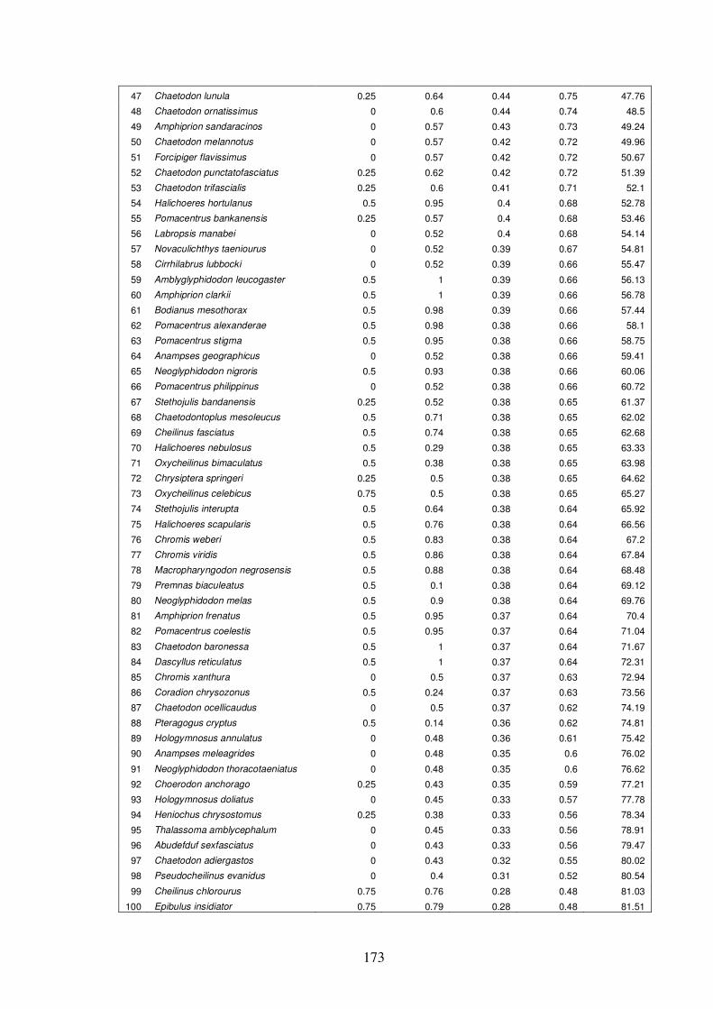
173
47 Chaetodon lunula 0.25 0.64 0.44 0.75 47.76
48 Chaetodon ornatissimus 0 0.6 0.44 0.74 48.5
49 Amphiprion sandaracinos 0 0.57 0.43 0.73 49.24
50 Chaetodon melannotus 0 0.57 0.42 0.72 49.96
51 Forcipiger flavissimus 0 0.57 0.42 0.72 50.67
52 Chaetodon punctatofasciatus 0.25 0.62 0.42 0.72 51.39
53 Chaetodon trifascialis 0.25 0.6 0.41 0.71 52.1
54 Halichoeres hortulanus 0.5 0.95 0.4 0.68 52.78
55 Pomacentrus bankanensis 0.25 0.57 0.4 0.68 53.46
56 Labropsis manabei 0 0.52 0.4 0.68 54.14
57 Novaculichthys taeniourus 0 0.52 0.39 0.67 54.81
58 Cirrhilabrus lubbocki 0 0.52 0.39 0.66 55.47
59 Amblyglyphidodon leucogaster 0.5 1 0.39 0.66 56.13
60 Amphiprion clarkii 0.5 1 0.39 0.66 56.78
61 Bodianus mesothorax 0.5 0.98 0.39 0.66 57.44
62 Pomacentrus alexanderae 0.5 0.98 0.38 0.66 58.1
63 Pomacentrus stigma 0.5 0.95 0.38 0.66 58.75
64 Anampses geographicus 0 0.52 0.38 0.66 59.41
65 Neoglyphidodon nigroris 0.5 0.93 0.38 0.66 60.06
66 Pomacentrus philippinus 0 0.52 0.38 0.66 60.72
67 Stethojulis bandanensis 0.25 0.52 0.38 0.65 61.37
68 Chaetodontoplus mesoleucus 0.5 0.71 0.38 0.65 62.02
69 Cheilinus fasciatus 0.5 0.74 0.38 0.65 62.68
70 Halichoeres nebulosus 0.5 0.29 0.38 0.65 63.33
71 Oxycheilinus bimaculatus 0.5 0.38 0.38 0.65 63.98
72 Chrysiptera springeri 0.25 0.5 0.38 0.65 64.62
73 Oxycheilinus celebicus 0.75 0.5 0.38 0.65 65.27
74 Stethojulis interupta 0.5 0.64 0.38 0.64 65.92
75 Halichoeres scapularis 0.5 0.76 0.38 0.64 66.56
76 Chromis weberi 0.5 0.83 0.38 0.64 67.2
77 Chromis viridis 0.5 0.86 0.38 0.64 67.84
78 Macropharyngodon negrosensis 0.5 0.88 0.38 0.64 68.48
79 Premnas biaculeatus 0.5 0.1 0.38 0.64 69.12
80 Neoglyphidodon melas 0.5 0.9 0.38 0.64 69.76
81 Amphiprion frenatus 0.5 0.95 0.37 0.64 70.4
82 Pomacentrus coelestis 0.5 0.95 0.37 0.64 71.04
83 Chaetodon baronessa 0.5 1 0.37 0.64 71.67
84 Dascyllus reticulatus 0.5 1 0.37 0.64 72.31
85 Chromis xanthura 0 0.5 0.37 0.63 72.94
86 Coradion chrysozonus 0.5 0.24 0.37 0.63 73.56
87 Chaetodon ocellicaudus 0 0.5 0.37 0.62 74.19
88 Pteragogus cryptus 0.5 0.14 0.36 0.62 74.81
89 Hologymnosus annulatus 0 0.48 0.36 0.61 75.42
90 Anampses meleagrides 0 0.48 0.35 0.6 76.02
91 Neoglyphidodon thoracotaeniatus 0 0.48 0.35 0.6 76.62
92 Choerodon anchorago 0.25 0.43 0.35 0.59 77.21
93 Hologymnosus doliatus 0 0.45 0.33 0.57 77.78
94 Heniochus chrysostomus 0.25 0.38 0.33 0.56 78.34
95 Thalassoma amblycephalum 0 0.45 0.33 0.56 78.91
96 Abudefduf sexfasciatus 0 0.43 0.33 0.56 79.47
97 Chaetodon adiergastos 0 0.43 0.32 0.55 80.02
98 Pseudocheilinus evanidus 0 0.4 0.31 0.52 80.54
99 Cheilinus chlorourus 0.75 0.76 0.28 0.48 81.03
100 Epibulus insidiator 0.75 0.79 0.28 0.48 81.51

174
101 Chromis atripes 0.25 0.26 0.28 0.48 81.99
102 Pomacentrus nigromarginatus 0 0.38 0.28 0.47 82.46
103 Oxycheilinus unifasciatus 0 0.36 0.27 0.46 82.93
104 Cheilinus oxycephalus 0 0.36 0.27 0.46 83.39
105 Chaetodon ulietensis 0.25 0.19 0.27 0.45 83.84
106 Cheiloprion labiatus 0.25 0.17 0.25 0.42 84.26
107 Chromis scotochiloptera 0 0.31 0.24 0.41 84.68
108 Oxycheilinus rhodochrous 0.25 0.14 0.24 0.4 85.08
109 Halichoeres marginatus 0 0.31 0.23 0.4 85.48
110 Cirrhilabrus cyanopleura 0.75 0.93 0.23 0.4 85.87
111 Amblyglyphidodon curacao 0.75 0.93 0.23 0.4 86.27
112 Chaetodon speculum 0 0.29 0.22 0.37 86.63
113 Genicanthus lamarck 0 0.29 0.21 0.37 87
114 Neopomacentrus anabatoides 0 0.29 0.21 0.36 87.36
115 Heniochus singularis 0 0.29 0.21 0.36 87.72
116 Pomacentrus nagasakiensis 0.25 0.07 0.21 0.36 88.07
117 Labroides bicolor 0 0.29 0.21 0.35 88.43
118 Chromis retrofasciata 0.75 1 0.21 0.35 88.78
119 Chrysiptera rollandi 0.75 1 0.21 0.35 89.13
120 Chrysiptera talboti 0.75 1 0.21 0.35 89.49
121 Halichoeres chloropterus 0.25 0.02 0.2 0.35 89.84
122 Halichoeres leucurus 0.25 0.02 0.2 0.35 90.18

175
Ave. Presence/Absence Ave.
Species Group B Group H Diss. % Cont. Cum. %
1 Centropyge vroliki 0 1 0.61 1.37 1.37
2 Chaetodon kleini 0 1 0.61 1.37 2.74
3 Chrysiptera unimaculata 1 0 0.61 1.37 4.1
4 Bodianus mesothorax 0 0.98 0.6 1.34 5.44
5 Labrichthys unilineatus 0 0.98 0.6 1.34 6.78
6 Halichoeres chloropterus 1 0.02 0.59 1.33 8.11
7 Pygoplites diacanthus 0 0.98 0.59 1.33 9.45
8 Chromis amboinensis 0 0.95 0.58 1.31 10.75
9 Halichoeres hortulanus 0 0.95 0.58 1.3 12.05
10 Abudefduf vaigiensis 0 0.95 0.58 1.3 13.35
11 Pomacentrus tripunctatus 1 0.07 0.57 1.27 14.62
12 Chromis margaritifer 0 0.93 0.57 1.27 15.89
13 Hemigymnus fasciatus 0 0.93 0.57 1.27 17.16
14 Pomacentrus nagasakiensis 1 0.07 0.56 1.27 18.43
15 Chaetodon selene 1 0.07 0.56 1.27 19.69
16 Pomacentrus lepidogenys 0 0.93 0.56 1.27 20.96
17 Plectroglyphidodon lacrymatus 0 0.9 0.55 1.23 22.19
18 Halichoeres argus 1 0.12 0.54 1.21 23.4
19 Coris gaimard 0 0.81 0.49 1.1 24.5
20 Halichoeres biocellatus 0 0.79 0.48 1.08 25.58
21 Pomacentrus chrysurus 1 0.21 0.48 1.07 26.65
22 Epibulus insidiator 0 0.79 0.47 1.07 27.72
23 Macropharyngodon meleagris 0 0.76 0.47 1.05 28.77
24 Gomphosus varius 0 0.76 0.46 1.03 29.8
25 Cheilinus trilobatus 0 0.71 0.43 0.97 30.77
26 Chromis atripectoralis 0 0.71 0.43 0.97 31.74
27 Chaetodon rafflesi 0 0.67 0.4 0.9 32.64
28 Halichoeres richmondi 0 0.67 0.4 0.9 33.54
29 Centropyge bicolor 0 0.64 0.38 0.86 34.39
30 Cheilio inermis 0 0.62 0.37 0.84 35.23
31 Chaetodon auriga 0 0.62 0.37 0.83 36.06
32 Chaetodon punctatofasciatus 0 0.62 0.37 0.83 36.89
33 Chaetodon trifascialis 0 0.6 0.36 0.8 37.69
34 Halichoeres chrysus 0 0.6 0.36 0.8 38.5
35 Chaetodon ornatissimus 0 0.6 0.35 0.79 39.29
36 Forcipiger flavissimus 0 0.57 0.34 0.76 40.05
37 Pomacentrus bankanensis 0 0.57 0.34 0.76 40.81
38 Labropsis manabei 0 0.52 0.32 0.72 41.53
39 Novaculichthys taeniourus 0 0.52 0.32 0.71 42.24
40 Stethojulis bandanensis 0 0.52 0.31 0.7 42.94
41 Amblyglyphidodon leucogaster 0.5 1 0.31 0.7 43.65
42 Amphiprion polymnus 0.5 0 0.31 0.7 44.35
43 Coris pictoides 0.5 0 0.31 0.7 45.05
44 Halichoeres hartzfeldii 0.5 0 0.31 0.7 45.75
45 Halichoeres margaritaceus 0.5 0 0.31 0.7 46.45
Appendix 4.3 Results of ‘similarity/distance percentage’ (SIMPER) analysis in PRIMER for group B vs. group H (see Materials and methods of Chapter 4). The average presence/absence of each species in groups B and H, average dissimilarity between groups (Ave. Diss.), percent contribution to dissimilarity (% Cont.) and cumulative % of dissimilarity (Cum. %) are shown. Data sorted according to increasing cumulative % of dissimilarity.
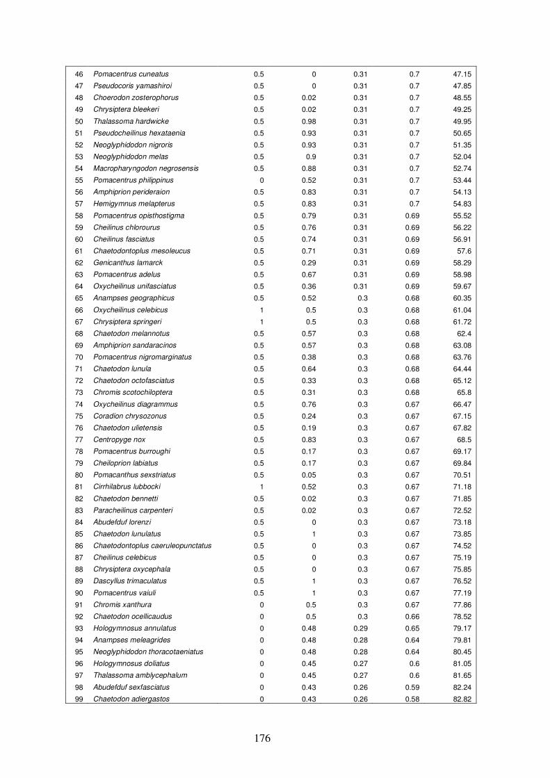
176
46 Pomacentrus cuneatus 0.5 0 0.31 0.7 47.15
47 Pseudocoris yamashiroi 0.5 0 0.31 0.7 47.85
48 Choerodon zosterophorus 0.5 0.02 0.31 0.7 48.55
49 Chrysiptera bleekeri 0.5 0.02 0.31 0.7 49.25
50 Thalassoma hardwicke 0.5 0.98 0.31 0.7 49.95
51 Pseudocheilinus hexataenia 0.5 0.93 0.31 0.7 50.65
52 Neoglyphidodon nigroris 0.5 0.93 0.31 0.7 51.35
53 Neoglyphidodon melas 0.5 0.9 0.31 0.7 52.04
54 Macropharyngodon negrosensis 0.5 0.88 0.31 0.7 52.74
55 Pomacentrus philippinus 0 0.52 0.31 0.7 53.44
56 Amphiprion perideraion 0.5 0.83 0.31 0.7 54.13
57 Hemigymnus melapterus 0.5 0.83 0.31 0.7 54.83
58 Pomacentrus opisthostigma 0.5 0.79 0.31 0.69 55.52
59 Cheilinus chlorourus 0.5 0.76 0.31 0.69 56.22
60 Cheilinus fasciatus 0.5 0.74 0.31 0.69 56.91
61 Chaetodontoplus mesoleucus 0.5 0.71 0.31 0.69 57.6
62 Genicanthus lamarck 0.5 0.29 0.31 0.69 58.29
63 Pomacentrus adelus 0.5 0.67 0.31 0.69 58.98
64 Oxycheilinus unifasciatus 0.5 0.36 0.31 0.69 59.67
65 Anampses geographicus 0.5 0.52 0.3 0.68 60.35
66 Oxycheilinus celebicus 1 0.5 0.3 0.68 61.04
67 Chrysiptera springeri 1 0.5 0.3 0.68 61.72
68 Chaetodon melannotus 0.5 0.57 0.3 0.68 62.4
69 Amphiprion sandaracinos 0.5 0.57 0.3 0.68 63.08
70 Pomacentrus nigromarginatus 0.5 0.38 0.3 0.68 63.76
71 Chaetodon lunula 0.5 0.64 0.3 0.68 64.44
72 Chaetodon octofasciatus 0.5 0.33 0.3 0.68 65.12
73 Chromis scotochiloptera 0.5 0.31 0.3 0.68 65.8
74 Oxycheilinus diagrammus 0.5 0.76 0.3 0.67 66.47
75 Coradion chrysozonus 0.5 0.24 0.3 0.67 67.15
76 Chaetodon ulietensis 0.5 0.19 0.3 0.67 67.82
77 Centropyge nox 0.5 0.83 0.3 0.67 68.5
78 Pomacentrus burroughi 0.5 0.17 0.3 0.67 69.17
79 Cheiloprion labiatus 0.5 0.17 0.3 0.67 69.84
80 Pomacanthus sexstriatus 0.5 0.05 0.3 0.67 70.51
81 Cirrhilabrus lubbocki 1 0.52 0.3 0.67 71.18
82 Chaetodon bennetti 0.5 0.02 0.3 0.67 71.85
83 Paracheilinus carpenteri 0.5 0.02 0.3 0.67 72.52
84 Abudefduf lorenzi 0.5 0 0.3 0.67 73.18
85 Chaetodon lunulatus 0.5 1 0.3 0.67 73.85
86 Chaetodontoplus caeruleopunctatus 0.5 0 0.3 0.67 74.52
87 Cheilinus celebicus 0.5 0 0.3 0.67 75.19
88 Chrysiptera oxycephala 0.5 0 0.3 0.67 75.85
89 Dascyllus trimaculatus 0.5 1 0.3 0.67 76.52
90 Pomacentrus vaiuli 0.5 1 0.3 0.67 77.19
91 Chromis xanthura 0 0.5 0.3 0.67 77.86
92 Chaetodon ocellicaudus 0 0.5 0.3 0.66 78.52
93 Hologymnosus annulatus 0 0.48 0.29 0.65 79.17
94 Anampses meleagrides 0 0.48 0.28 0.64 79.81
95 Neoglyphidodon thoracotaeniatus 0 0.48 0.28 0.64 80.45
96 Hologymnosus doliatus 0 0.45 0.27 0.6 81.05
97 Thalassoma amblycephalum 0 0.45 0.27 0.6 81.65
98 Abudefduf sexfasciatus 0 0.43 0.26 0.59 82.24
99 Chaetodon adiergastos 0 0.43 0.26 0.58 82.82

177
100 Choerodon anchorago 0 0.43 0.26 0.58 83.4
101 Pseudocheilinus evanidus 0 0.4 0.25 0.55 83.96
102 Oxycheilinus bimaculatus 0 0.38 0.23 0.52 84.48
103 Heniochus chrysostomus 0 0.38 0.22 0.5 84.98
104 Cheilinus oxycephalus 0 0.36 0.22 0.49 85.47
105 Stethojulis interupta 1 0.64 0.21 0.47 85.94
106 Halichoeres marginatus 0 0.31 0.19 0.42 86.36
107 Chromis analis 1 0.71 0.18 0.39 86.75
108 Halichoeres nebulosus 0 0.29 0.17 0.39 87.14
109 Halichoeres solorensis 1 0.71 0.17 0.39 87.53
110 Chaetodon speculum 0 0.29 0.17 0.39 87.92
111 Neopomacentrus anabatoides 0 0.29 0.17 0.38 88.3
112 Heniochus singularis 0 0.29 0.17 0.38 88.69
113 Labroides bicolor 0 0.29 0.17 0.38 89.06
114 Chromis atripes 0 0.26 0.16 0.35 89.42
115 Anampses twistii 0 0.26 0.16 0.35 89.77
116 Halichoeres scapularis 1 0.76 0.15 0.33 90.09
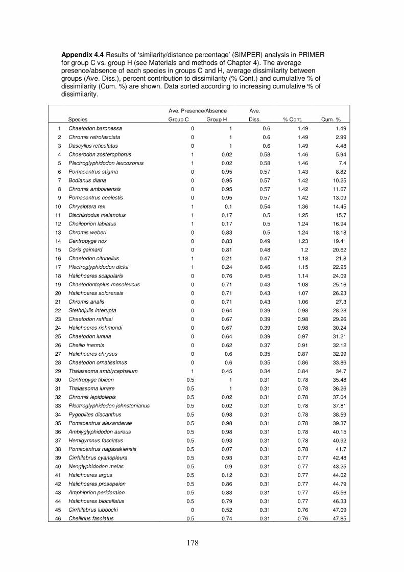
178
Ave. Presence/Absence Ave.
Species Group C Group H Diss. % Cont. Cum. %
1 Chaetodon baronessa 0 1 0.6 1.49 1.49
2 Chromis retrofasciata 0 1 0.6 1.49 2.99
3 Dascyllus reticulatus 0 1 0.6 1.49 4.48
4 Choerodon zosterophorus 1 0.02 0.58 1.46 5.94
5 Plectroglyphidodon leucozonus 1 0.02 0.58 1.46 7.4
6 Pomacentrus stigma 0 0.95 0.57 1.43 8.82
7 Bodianus diana 0 0.95 0.57 1.42 10.25
8 Chromis amboinensis 0 0.95 0.57 1.42 11.67
9 Pomacentrus coelestis 0 0.95 0.57 1.42 13.09
10 Chrysiptera rex 1 0.1 0.54 1.36 14.45
11 Dischistodus melanotus 1 0.17 0.5 1.25 15.7
12 Cheiloprion labiatus 1 0.17 0.5 1.24 16.94
13 Chromis weberi 0 0.83 0.5 1.24 18.18
14 Centropyge nox 0 0.83 0.49 1.23 19.41
15 Coris gaimard 0 0.81 0.48 1.2 20.62
16 Chaetodon citrinellus 1 0.21 0.47 1.18 21.8
17 Plectroglyphidodon dickii 1 0.24 0.46 1.15 22.95
18 Halichoeres scapularis 0 0.76 0.45 1.14 24.09
19 Chaetodontoplus mesoleucus 0 0.71 0.43 1.08 25.16
20 Halichoeres solorensis 0 0.71 0.43 1.07 26.23
21 Chromis analis 0 0.71 0.43 1.06 27.3
22 Stethojulis interupta 0 0.64 0.39 0.98 28.28
23 Chaetodon rafflesi 0 0.67 0.39 0.98 29.26
24 Halichoeres richmondi 0 0.67 0.39 0.98 30.24
25 Chaetodon lunula 0 0.64 0.39 0.97 31.21
26 Cheilio inermis 0 0.62 0.37 0.91 32.12
27 Halichoeres chrysus 0 0.6 0.35 0.87 32.99
28 Chaetodon ornatissimus 0 0.6 0.35 0.86 33.86
29 Thalassoma amblycephalum 1 0.45 0.34 0.84 34.7
30 Centropyge tibicen 0.5 1 0.31 0.78 35.48
31 Thalassoma lunare 0.5 1 0.31 0.78 36.26
32 Chromis lepidolepis 0.5 0.02 0.31 0.78 37.04
33 Plectroglyphidodon johnstonianus 0.5 0.02 0.31 0.78 37.81
34 Pygoplites diacanthus 0.5 0.98 0.31 0.78 38.59
35 Pomacentrus alexanderae 0.5 0.98 0.31 0.78 39.37
36 Amblyglyphidodon aureus 0.5 0.98 0.31 0.78 40.15
37 Hemigymnus fasciatus 0.5 0.93 0.31 0.78 40.92
38 Pomacentrus nagasakiensis 0.5 0.07 0.31 0.78 41.7
39 Cirrhilabrus cyanopleura 0.5 0.93 0.31 0.77 42.48
40 Neoglyphidodon melas 0.5 0.9 0.31 0.77 43.25
41 Halichoeres argus 0.5 0.12 0.31 0.77 44.02
42 Halichoeres prosopeion 0.5 0.86 0.31 0.77 44.79
43 Amphiprion perideraion 0.5 0.83 0.31 0.77 45.56
44 Halichoeres biocellatus 0.5 0.79 0.31 0.77 46.33
45 Cirrhilabrus lubbocki 0 0.52 0.31 0.76 47.09
46 Cheilinus fasciatus 0.5 0.74 0.31 0.76 47.85
Appendix 4.4 Results of ‘similarity/distance percentage’ (SIMPER) analysis in PRIMER for group C vs. group H (see Materials and methods of Chapter 4). The average presence/absence of each species in groups C and H, average dissimilarity between groups (Ave. Diss.), percent contribution to dissimilarity (% Cont.) and cumulative % of dissimilarity (Cum. %) are shown. Data sorted according to increasing cumulative % of dissimilarity.

179
47 Pomacentrus philippinus 0 0.52 0.3 0.76 48.61
48 Halichoeres marginatus 0.5 0.31 0.3 0.76 49.37
49 Centropyge bicolor 0.5 0.64 0.3 0.75 50.13
50 Chaetodon auriga 0.5 0.62 0.3 0.75 50.88
51 Forcipiger flavissimus 0.5 0.57 0.3 0.75 51.63
52 Labropsis manabei 0.5 0.52 0.3 0.75 52.38
53 Chrysiptera springeri 0 0.5 0.3 0.75 53.13
54 Novaculichthys taeniourus 0.5 0.52 0.3 0.75 53.88
55 Oxycheilinus celebicus 0 0.5 0.3 0.75 54.62
56 Anampses geographicus 0.5 0.52 0.3 0.75 55.37
57 Stethojulis bandanensis 0.5 0.52 0.3 0.75 56.12
58 Chromis xanthura 0.5 0.5 0.3 0.75 56.86
59 Anampses meleagrides 0.5 0.48 0.3 0.74 57.61
60 Amphiprion sandaracinos 0.5 0.57 0.3 0.74 58.35
61 Chaetodon trifascialis 0.5 0.6 0.3 0.74 59.09
62 Oxycheilinus unifasciatus 0.5 0.36 0.3 0.74 59.83
63 Cheilinus oxycephalus 0.5 0.36 0.29 0.74 60.56
64 Chromis atripectoralis 0.5 0.71 0.29 0.73 61.3
65 Cheilinus trilobatus 0.5 0.71 0.29 0.73 62.03
66 Epibulus insidiator 0.5 0.79 0.29 0.73 62.76
67 Centropyge bispinosus 0.5 0.24 0.29 0.73 63.49
68 Bodianus axillaris 0.5 0.21 0.29 0.73 64.21
69 Chaetodon ocellicaudus 0 0.5 0.29 0.72 64.94
70 Chromis viridis 0.5 0.86 0.29 0.72 65.66
71 Pomacanthus semicirculatus 0.5 0.12 0.29 0.72 66.38
72 Chaetodon unimaculatus 0.5 0.07 0.29 0.72 67.1
73 Abudefduf vaigiensis 0.5 0.95 0.29 0.72 67.82
74 Halichoeres leucurus 0.5 0.02 0.29 0.71 68.53
75 Halichoeres podostigma 0.5 0.98 0.29 0.71 69.25
76 Dascyllus aruanus 0.5 0.98 0.29 0.71 69.96
77 Thalassoma quinquevittatum 0.5 0.02 0.29 0.71 70.68
78 Chromis ternatensis 0.5 1 0.29 0.71 71.39
79 Chromis xanthochira 0.5 0 0.29 0.71 72.1
80 Cirrhilabrus rubripinnis 0.5 0 0.29 0.71 72.82
81 Dascyllus trimaculatus 0.5 1 0.29 0.71 73.53
82 Labropsis xanthonota 0.5 0 0.29 0.71 74.24
83 Thalassoma purpureum 0.5 0 0.29 0.71 74.96
84 Hologymnosus annulatus 0 0.48 0.28 0.71 75.66
85 Neoglyphidodon thoracotaeniatus 0 0.48 0.28 0.7 76.36
86 Pomacentrus bankanensis 1 0.57 0.26 0.66 77.02
87 Hologymnosus doliatus 0 0.45 0.26 0.66 77.68
88 Chaetodon melannotus 1 0.57 0.26 0.66 78.34
89 Abudefduf sexfasciatus 0 0.43 0.26 0.65 78.98
90 Chaetodon adiergastos 0 0.43 0.25 0.64 79.62
91 Choerodon anchorago 0 0.43 0.25 0.63 80.25
92 Pseudocheilinus evanidus 0 0.4 0.24 0.6 80.86
93 Chaetodon punctatofasciatus 1 0.62 0.24 0.59 81.45
94 Oxycheilinus bimaculatus 0 0.38 0.23 0.57 82.01
95 Pomacentrus nigromarginatus 0 0.38 0.22 0.55 82.56
96 Heniochus chrysostomus 0 0.38 0.22 0.55 83.12
97 Pomacentrus adelus 1 0.67 0.2 0.51 83.62
98 Chaetodon octofasciatus 0 0.33 0.2 0.5 84.12
99 Chromis scotochiloptera 0 0.31 0.19 0.47 84.6
100 Halichoeres nebulosus 0 0.29 0.17 0.43 85.02
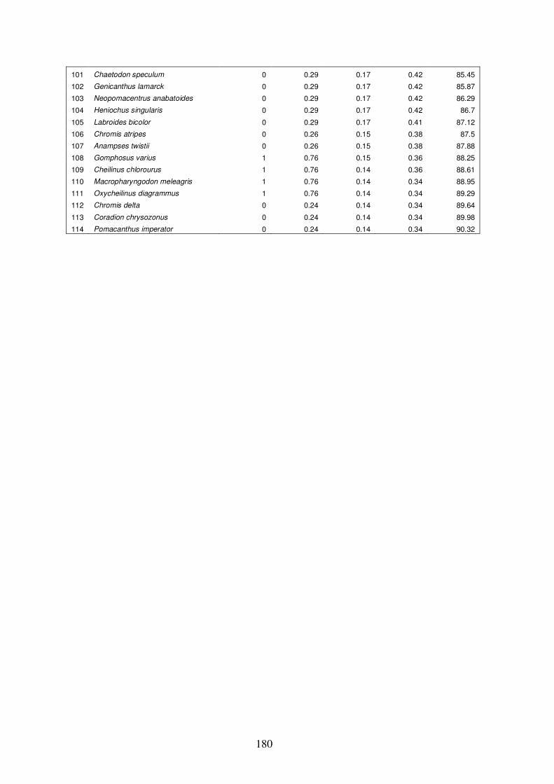
180
101 Chaetodon speculum 0 0.29 0.17 0.42 85.45
102 Genicanthus lamarck 0 0.29 0.17 0.42 85.87
103 Neopomacentrus anabatoides 0 0.29 0.17 0.42 86.29
104 Heniochus singularis 0 0.29 0.17 0.42 86.7
105 Labroides bicolor 0 0.29 0.17 0.41 87.12
106 Chromis atripes 0 0.26 0.15 0.38 87.5
107 Anampses twistii 0 0.26 0.15 0.38 87.88
108 Gomphosus varius 1 0.76 0.15 0.36 88.25
109 Cheilinus chlorourus 1 0.76 0.14 0.36 88.61
110 Macropharyngodon meleagris 1 0.76 0.14 0.34 88.95
111 Oxycheilinus diagrammus 1 0.76 0.14 0.34 89.29
112 Chromis delta 0 0.24 0.14 0.34 89.64
113 Coradion chrysozonus 0 0.24 0.14 0.34 89.98
114 Pomacanthus imperator 0 0.24 0.14 0.34 90.32

181
Ave. Presence/Absence Ave.
Species Group E Group H Diss. % Cont. Cum. %
1 Pomacentrus cuneatus 1 0 0.59 1.66 1.66
2 Pomacentrus smithi 1 0 0.59 1.66 3.31
3 Pomacentrus vaiuli 0 1 0.59 1.66 4.97
4 Pomacentrus nagasakiensis 1 0.07 0.54 1.53 6.5
5 Chaetodon vagabundus 0 0.83 0.48 1.37 7.87
6 Halichoeres biocellatus 0 0.79 0.46 1.3 9.17
7 Macropharyngodon meleagris 0 0.76 0.45 1.27 10.44
8 Gomphosus varius 0 0.76 0.44 1.25 11.7
9 Neopomacentrus anabatoides 1 0.29 0.42 1.19 12.89
10 Halichoeres solorensis 0 0.71 0.42 1.18 14.07
11 Chaetodon lunulatus 0.33 1 0.4 1.13 15.21
12 Centropyge tibicen 0.33 1 0.39 1.11 16.31
13 Chaetodon octofasciatus 1 0.33 0.39 1.1 17.41
14 Chromis margaritifer 0.33 0.93 0.39 1.09 18.5
15 Hemigymnus fasciatus 0.33 0.93 0.39 1.09 19.59
16 Stethojulis interupta 0 0.64 0.39 1.09 20.68
17 Hemiglyphidodon plagiometapon 0.67 0 0.38 1.07 21.75
18 Neoglyphidodon melas 0.33 0.9 0.38 1.07 22.82
19 Coradion melanopus 0.67 0.07 0.37 1.04 23.86
20 Centropyge bicolor 0 0.64 0.37 1.04 24.9
21 Amphiprion perideraion 0.33 0.83 0.37 1.03 25.93
22 Pomacentrus burroughi 0.67 0.17 0.37 1.03 26.96
23 Hemigymnus melapterus 0.33 0.83 0.36 1.03 27.99
24 Cheilio inermis 0 0.62 0.36 1.01 29
25 Chaetodon auriga 0 0.62 0.36 1.01 30.01
26 Chaetodon punctatofasciatus 0 0.62 0.36 1 31.02
27 Cheilinus chlorourus 0.33 0.76 0.35 0.99 32
28 Coris gaimard 0.33 0.81 0.35 0.98 32.98
29 Chaetodon trifascialis 0 0.6 0.35 0.97 33.95
30 Halichoeres chrysus 0 0.6 0.34 0.97 34.92
31 Chaetodon oxycephalus 0.67 0.21 0.34 0.97 35.89
32 Oxycheilinus diagrammus 0.33 0.76 0.34 0.96 36.85
33 Chaetodon ornatissimus 0 0.6 0.34 0.96 37.81
34 Choerodon anchorago 1 0.43 0.34 0.96 38.77
35 Cheilinus trilobatus 0.33 0.71 0.34 0.95 39.72
36 Chaetodon speculum 0.67 0.29 0.33 0.93 40.65
37 Chromis scotochiloptera 0.67 0.31 0.33 0.93 41.58
38 Forcipiger flavissimus 0 0.57 0.33 0.92 42.51
39 Pomacentrus bankanensis 0 0.57 0.33 0.92 43.43
40 Chaetodon lunula 0.33 0.64 0.32 0.91 44.34
41 Pomacentrus adelus 0.33 0.67 0.32 0.91 45.25
42 Pomacentrus nigromarginatus 0.67 0.38 0.32 0.89 46.14
43 Labropsis manabei 0 0.52 0.31 0.87 47.01
44 Hologymnosus doliatus 0.67 0.45 0.31 0.86 47.88
45 Chaetodon melannotus 0.33 0.57 0.31 0.86 48.74
Appendix 4.5 Results of ‘similarity/distance percentage’ (SIMPER) analysis in PRIMER for group E vs. group H (see Materials and methods of Chapter 4). The average presence/absence of each species in groups E and H, average dissimilarity between groups (Ave. Diss.), percent contribution to dissimilarity (% Cont.) and cumulative % of dissimilarity (Cum. %) are shown. Data sorted according to increasing cumulative % of dissimilarity.
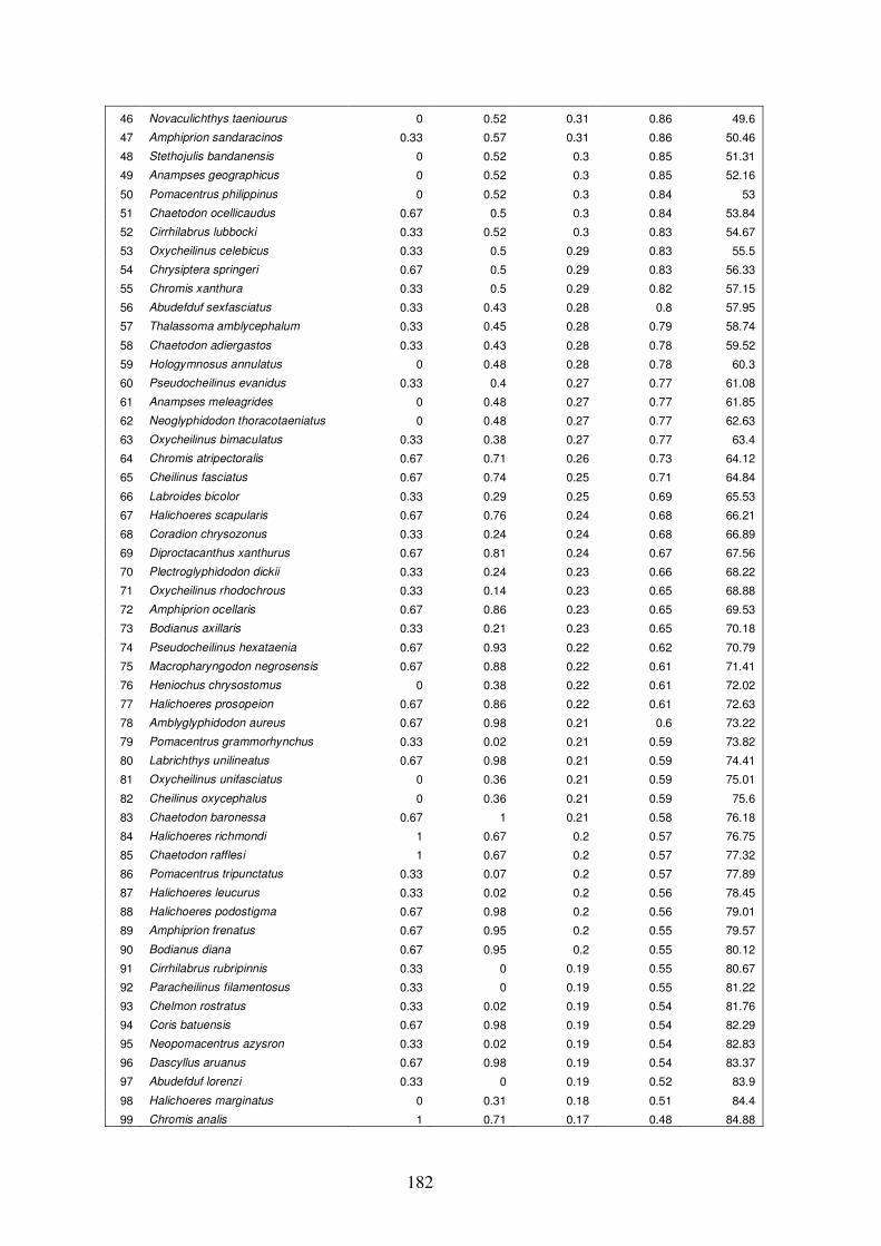
182
46 Novaculichthys taeniourus 0 0.52 0.31 0.86 49.6
47 Amphiprion sandaracinos 0.33 0.57 0.31 0.86 50.46
48 Stethojulis bandanensis 0 0.52 0.3 0.85 51.31
49 Anampses geographicus 0 0.52 0.3 0.85 52.16
50 Pomacentrus philippinus 0 0.52 0.3 0.84 53
51 Chaetodon ocellicaudus 0.67 0.5 0.3 0.84 53.84
52 Cirrhilabrus lubbocki 0.33 0.52 0.3 0.83 54.67
53 Oxycheilinus celebicus 0.33 0.5 0.29 0.83 55.5
54 Chrysiptera springeri 0.67 0.5 0.29 0.83 56.33
55 Chromis xanthura 0.33 0.5 0.29 0.82 57.15
56 Abudefduf sexfasciatus 0.33 0.43 0.28 0.8 57.95
57 Thalassoma amblycephalum 0.33 0.45 0.28 0.79 58.74
58 Chaetodon adiergastos 0.33 0.43 0.28 0.78 59.52
59 Hologymnosus annulatus 0 0.48 0.28 0.78 60.3
60 Pseudocheilinus evanidus 0.33 0.4 0.27 0.77 61.08
61 Anampses meleagrides 0 0.48 0.27 0.77 61.85
62 Neoglyphidodon thoracotaeniatus 0 0.48 0.27 0.77 62.63
63 Oxycheilinus bimaculatus 0.33 0.38 0.27 0.77 63.4
64 Chromis atripectoralis 0.67 0.71 0.26 0.73 64.12
65 Cheilinus fasciatus 0.67 0.74 0.25 0.71 64.84
66 Labroides bicolor 0.33 0.29 0.25 0.69 65.53
67 Halichoeres scapularis 0.67 0.76 0.24 0.68 66.21
68 Coradion chrysozonus 0.33 0.24 0.24 0.68 66.89
69 Diproctacanthus xanthurus 0.67 0.81 0.24 0.67 67.56
70 Plectroglyphidodon dickii 0.33 0.24 0.23 0.66 68.22
71 Oxycheilinus rhodochrous 0.33 0.14 0.23 0.65 68.88
72 Amphiprion ocellaris 0.67 0.86 0.23 0.65 69.53
73 Bodianus axillaris 0.33 0.21 0.23 0.65 70.18
74 Pseudocheilinus hexataenia 0.67 0.93 0.22 0.62 70.79
75 Macropharyngodon negrosensis 0.67 0.88 0.22 0.61 71.41
76 Heniochus chrysostomus 0 0.38 0.22 0.61 72.02
77 Halichoeres prosopeion 0.67 0.86 0.22 0.61 72.63
78 Amblyglyphidodon aureus 0.67 0.98 0.21 0.6 73.22
79 Pomacentrus grammorhynchus 0.33 0.02 0.21 0.59 73.82
80 Labrichthys unilineatus 0.67 0.98 0.21 0.59 74.41
81 Oxycheilinus unifasciatus 0 0.36 0.21 0.59 75.01
82 Cheilinus oxycephalus 0 0.36 0.21 0.59 75.6
83 Chaetodon baronessa 0.67 1 0.21 0.58 76.18
84 Halichoeres richmondi 1 0.67 0.2 0.57 76.75
85 Chaetodon rafflesi 1 0.67 0.2 0.57 77.32
86 Pomacentrus tripunctatus 0.33 0.07 0.2 0.57 77.89
87 Halichoeres leucurus 0.33 0.02 0.2 0.56 78.45
88 Halichoeres podostigma 0.67 0.98 0.2 0.56 79.01
89 Amphiprion frenatus 0.67 0.95 0.2 0.55 79.57
90 Bodianus diana 0.67 0.95 0.2 0.55 80.12
91 Cirrhilabrus rubripinnis 0.33 0 0.19 0.55 80.67
92 Paracheilinus filamentosus 0.33 0 0.19 0.55 81.22
93 Chelmon rostratus 0.33 0.02 0.19 0.54 81.76
94 Coris batuensis 0.67 0.98 0.19 0.54 82.29
95 Neopomacentrus azysron 0.33 0.02 0.19 0.54 82.83
96 Dascyllus aruanus 0.67 0.98 0.19 0.54 83.37
97 Abudefduf lorenzi 0.33 0 0.19 0.52 83.9
98 Halichoeres marginatus 0 0.31 0.18 0.51 84.4
99 Chromis analis 1 0.71 0.17 0.48 84.88

183
100 Halichoeres nebulosus 0 0.29 0.17 0.47 85.35
101 Genicanthus lamarck 0 0.29 0.17 0.47 85.82
102 Chaetodontoplus mesoleucus 1 0.71 0.16 0.46 86.29
103 Heniochus singularis 0 0.29 0.16 0.46 86.75
104 Chromis atripes 0 0.26 0.15 0.43 87.18
105 Anampses twistii 0 0.26 0.15 0.42 87.6
106 Centropyge bispinosus 0 0.24 0.14 0.38 87.98
107 Chromis delta 0 0.24 0.14 0.38 88.36
108 Pomacanthus imperator 0 0.24 0.13 0.38 88.74
109 Epibulus insidiator 1 0.79 0.13 0.37 89.11
110 Pomacentrus opisthostigma 1 0.79 0.13 0.36 89.47
111 Pomacentrus chrysurus 0 0.21 0.13 0.36 89.83
112 Thalassoma jansenii 0 0.21 0.13 0.36 90.18

184
Ave. Presence/Absence Ave.
Species Group F Group H Diss. % Cont. Cum. %
1 Chrysiptera cyanea 1 0 0.56 1.63 1.63
2 Chromis ovatiformis 1 0.02 0.54 1.59 3.21
3 Chaetodon bennetti 1 0.02 0.54 1.59 4.8
4 Chromis caudalis 1 0.07 0.52 1.51 6.31
5 Chrysiptera rex 1 0.1 0.51 1.48 7.79
6 Neoglyphidodon melas 0 0.9 0.5 1.47 9.25
7 Chromis viridis 0 0.86 0.47 1.38 10.63
8 Bodianus axillaris 1 0.21 0.44 1.29 11.92
9 Chaetodon xanthurus 1 0.21 0.44 1.29 13.21
10 Halichoeres biocellatus 0 0.79 0.44 1.28 14.49
11 Macropharyngodon meleagris 0 0.76 0.43 1.25 15.74
12 Cheilinus chlorourus 0 0.76 0.42 1.24 16.98
13 Centropyge tibicen 0.25 1 0.42 1.22 18.2
14 Dascyllus aruanus 0.25 0.98 0.41 1.2 19.4
15 Bodianus diana 0.25 0.95 0.41 1.2 20.6
16 Abudefduf vaigiensis 0.25 0.95 0.41 1.19 21.78
17 Halichoeres solorensis 0 0.71 0.4 1.16 22.95
18 Chromis atripectoralis 0 0.71 0.39 1.15 24.1
19 Macropharyngodon negrosensis 0.25 0.88 0.39 1.13 25.23
20 Amphiprion ocellaris 0.25 0.86 0.38 1.11 26.34
21 Halichoeres binotopsis 0.75 0.14 0.38 1.11 27.45
22 Amphiprion perideraion 0.25 0.83 0.37 1.09 28.54
23 Diproctacanthus xanthurus 0.25 0.81 0.37 1.08 29.61
24 Coris gaimard 0.25 0.81 0.37 1.07 30.68
25 Stethojulis interupta 0 0.64 0.37 1.07 31.75
26 Halichoeres scapularis 0.25 0.76 0.35 1.03 32.78
27 Pomacentrus nigromarginatus 1 0.38 0.35 1.03 33.8
28 Cheilio inermis 0 0.62 0.34 1 34.8
29 Chaetodontoplus mesoleucus 0.25 0.71 0.34 0.99 35.79
30 Cheilinus trilobatus 0.25 0.71 0.34 0.99 36.78
31 Halichoeres chrysus 0 0.6 0.33 0.95 37.73
32 Halichoeres richmondi 0.25 0.67 0.32 0.94 38.67
33 Chaetodon adiergastos 0.75 0.43 0.3 0.87 39.54
34 Novaculichthys taeniourus 0 0.52 0.29 0.85 40.39
35 Labropsis manabei 0.25 0.52 0.29 0.83 41.23
36 Cirrhilabrus lubbocki 0 0.52 0.29 0.83 42.06
37 Chromis xanthura 1 0.5 0.29 0.83 42.89
38 Amphiprion clarkii 0.5 1 0.28 0.83 43.72
39 Chromis analis 0.5 0.71 0.28 0.82 44.54
40 Coris batuensis 0.5 0.98 0.28 0.82 45.37
41 Anampses geographicus 0.25 0.52 0.28 0.82 46.19
42 Halichoeres melanurus 0.5 0.88 0.28 0.82 47.01
43 Hemigymnus melapterus 0.5 0.83 0.28 0.82 47.83
44 Thalassoma jansenii 0.5 0.21 0.28 0.82 48.65
45 Plectroglyphidodon dickii 0.5 0.24 0.28 0.82 49.47
46 Chromis atripes 0.5 0.26 0.28 0.82 50.28
Appendix 4.6 Results of ‘similarity/distance percentage’ (SIMPER) analysis in PRIMER for group F vs. group H (see Materials and methods of Chapter 4). The average presence/absence of each species in groups F and H, average dissimilarity between groups (Ave. Diss.), percent contribution to dissimilarity (% Cont.) and cumulative % of dissimilarity (Cum. %) are shown. Data sorted according to increasing cumulative % of dissimilarity.

185
47 Chaetodon melannotus 0.5 0.57 0.28 0.81 51.1
48 Chrysiptera springeri 0.25 0.5 0.28 0.81 51.91
49 Oxycheilinus celebicus 0.25 0.5 0.28 0.81 52.73
50 Stethojulis bandanensis 0.5 0.52 0.28 0.81 53.54
51 Chaetodon ocellicaudus 0.5 0.5 0.28 0.81 54.35
52 Pseudocheilinus evanidus 0.5 0.4 0.28 0.81 55.16
53 Chaetodon lunula 0.5 0.64 0.28 0.81 55.97
54 Chaetodon octofasciatus 0.5 0.33 0.28 0.81 56.78
55 Chaetodon trifascialis 0.5 0.6 0.28 0.81 57.59
56 Neopomacentrus anabatoides 0.5 0.29 0.28 0.81 58.4
57 Heniochus chrysostomus 0.5 0.38 0.28 0.81 59.21
58 Halichoeres marginatus 0.5 0.31 0.28 0.81 60.02
59 Halichoeres argus 0.5 0.12 0.28 0.81 60.82
60 Chaetodon citrinellus 0.5 0.21 0.28 0.8 61.63
61 Chaetodon speculum 0.5 0.29 0.28 0.8 62.43
62 Labroides bicolor 0.5 0.29 0.27 0.8 63.23
63 Chaetodon ulietensis 0.5 0.19 0.27 0.8 64.03
64 Pomacentrus philippinus 1 0.52 0.27 0.8 64.83
65 Anampses meleagrides 0.25 0.48 0.27 0.79 65.62
66 Neoglyphidodon thoracotaeniatus 0.25 0.48 0.27 0.79 66.4
67 Hologymnosus annulatus 0 0.48 0.26 0.77 67.17
68 Pomacentrus bankanensis 0.75 0.57 0.26 0.77 67.94
69 Hologymnosus doliatus 0.25 0.45 0.26 0.76 68.7
70 Thalassoma amblycephalum 0.25 0.45 0.26 0.76 69.46
71 Chaetodon ornatissimus 0.75 0.6 0.26 0.75 70.21
72 Forcipiger flavissimus 1 0.57 0.25 0.72 70.93
73 Amphiprion sandaracinos 1 0.57 0.24 0.7 71.64
74 Abudefduf sexfasciatus 0 0.43 0.24 0.7 72.34
75 Cheilinus oxycephalus 0.25 0.36 0.24 0.69 73.03
76 Choerodon anchorago 0 0.43 0.24 0.69 73.72
77 Chaetodon rafflesi 0.75 0.67 0.23 0.68 74.41
78 Chaetodon punctatofasciatus 1 0.62 0.22 0.64 75.05
79 Cheilinus fasciatus 0.75 0.74 0.22 0.63 75.68
80 Halichoeres nebulosus 0.25 0.29 0.22 0.63 76.31
81 Chaetodon auriga 1 0.62 0.22 0.63 76.95
82 Anampses twistii 0.25 0.26 0.22 0.63 77.57
83 Heniochus singularis 0.25 0.29 0.21 0.63 78.2
84 Oxycheilinus bimaculatus 0 0.38 0.21 0.62 78.82
85 Centropyge bicolor 1 0.64 0.21 0.61 79.43
86 Oxycheilinus diagrammus 0.75 0.76 0.2 0.59 80.02
87 Oxycheilinus unifasciatus 0 0.36 0.2 0.58 80.6
88 Chaetodon oxycephalus 0.25 0.21 0.2 0.58 81.18
89 Pomacentrus chrysurus 0.25 0.21 0.2 0.58 81.76
90 Labropsis alleni 0.25 0.21 0.19 0.57 82.33
91 Dascyllus melanurus 0.25 0.19 0.19 0.55 82.88
92 Pomacentrus adelus 1 0.67 0.19 0.55 83.43
93 Forcipiger longirostris 0.25 0.19 0.19 0.55 83.98
94 Chromis weberi 0.75 0.83 0.19 0.54 84.52
95 Pomacentrus burroughi 0.25 0.17 0.19 0.54 85.06
96 Chromis scotochiloptera 0 0.31 0.18 0.52 85.58
97 Pomacentrus coelestis 0.75 0.95 0.16 0.47 86.05
98 Chromis margaritifer 0.75 0.93 0.16 0.46 86.51
99 Genicanthus lamarck 0 0.29 0.16 0.46 86.97
100 Hemigymnus fasciatus 0.75 0.93 0.16 0.45 87.42
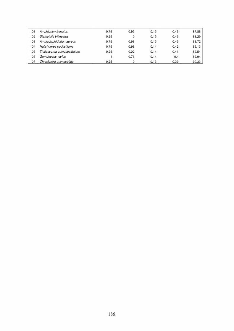
186
101 Amphiprion frenatus 0.75 0.95 0.15 0.43 87.86
102 Stethojulis trilineatus 0.25 0 0.15 0.43 88.29
103 Amblyglyphidodon aureus 0.75 0.98 0.15 0.43 88.72
104 Halichoeres podostigma 0.75 0.98 0.14 0.42 89.13
105 Thalassoma quinquevittatum 0.25 0.02 0.14 0.41 89.54
106 Gomphosus varius 1 0.76 0.14 0.4 89.94
107 Chrysiptera unimaculata 0.25 0 0.13 0.39 90.33
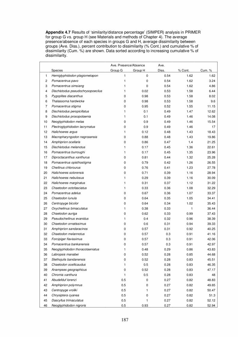
187
Ave. Presence/Absence Ave.
Species Group G Group H Diss. % Cont. Cum. %
1 Hemiglyphidodon plagiometapon 1 0 0.54 1.62 1.62
2 Pomacentrus pavo 1 0 0.54 1.62 3.24
3 Pomacentrus simsiang 1 0 0.54 1.62 4.86
4 Dischistodus pseudochrysopoecilus 1 0.02 0.53 1.58 6.44
5 Pygoplites diacanthus 0 0.98 0.53 1.58 8.02
6 Thalassoma hardwicke 0 0.98 0.53 1.58 9.6
7 Pomacentrus stigma 0 0.95 0.52 1.55 11.15
8 Dischistodus perspicillatus 1 0.1 0.49 1.47 12.62
9 Dischistodus prosopotaenia 1 0.1 0.49 1.46 14.08
10 Neoglyphidodon melas 0 0.9 0.49 1.46 15.54
11 Plectroglyphidodon lacrymatus 0 0.9 0.49 1.46 17
12 Halichoeres argus 1 0.12 0.48 1.43 18.43
13 Macropharyngodon negrosensis 0 0.88 0.48 1.43 19.86
14 Amphiprion ocellaris 0 0.86 0.47 1.4 21.25
15 Dischistodus melanotus 1 0.17 0.45 1.36 22.61
16 Pomacentrus burroughi 1 0.17 0.45 1.35 23.96
17 Diproctacanthus xanthurus 0 0.81 0.44 1.32 25.28
18 Pomacentrus opisthostigma 0 0.79 0.42 1.26 26.55
19 Cheilinus chlorourus 0 0.76 0.41 1.23 27.78
20 Halichoeres solorensis 0 0.71 0.39 1.16 28.94
21 Halichoeres nebulosus 1 0.29 0.39 1.16 30.09
22 Halichoeres marginatus 1 0.31 0.37 1.12 31.22
23 Chaetodon octofasciatus 1 0.33 0.36 1.08 32.29
24 Pomacentrus adelus 0 0.67 0.36 1.07 33.37
25 Chaetodon lunula 0 0.64 0.35 1.05 34.41
26 Centropyge bicolor 0 0.64 0.34 1.02 35.43
27 Oxycheilinus bimaculatus 1 0.38 0.33 1 36.44
28 Chaetodon auriga 0 0.62 0.33 0.99 37.43
29 Pseudocheilinus evanidus 1 0.4 0.32 0.96 38.39
30 Chaetodon ornatissimus 0 0.6 0.31 0.94 39.33
31 Amphiprion sandaracinos 0 0.57 0.31 0.92 40.25
32 Chaetodon melannotus 0 0.57 0.3 0.91 41.16
33 Forcipiger flavissimus 0 0.57 0.3 0.91 42.06
34 Pomacentrus bankanensis 0 0.57 0.3 0.91 42.97
35 Neoglyphidodon thoracotaeniatus 1 0.48 0.29 0.86 43.83
36 Labropsis manabei 0 0.52 0.28 0.85 44.68
37 Stethojulis bandanensis 0 0.52 0.28 0.83 45.51
38 Chaetodon ocellicaudus 1 0.5 0.28 0.83 46.35
39 Anampses geographicus 0 0.52 0.28 0.83 47.17
40 Chromis xanthura 1 0.5 0.28 0.83 48
41 Abudefduf lorenzi 0.5 0 0.27 0.82 48.83
42 Amphiprion polymnus 0.5 0 0.27 0.82 49.65
43 Centropyge vroliki 0.5 1 0.27 0.82 50.47
44 Chrysiptera cyanea 0.5 0 0.27 0.82 51.3
45 Dascyllus trimaculatus 0.5 1 0.27 0.82 52.12
46 Neoglyphidodon nigroris 0.5 0.93 0.27 0.82 52.94
Appendix 4.7 Results of ‘similarity/distance percentage’ (SIMPER) analysis in PRIMER for group G vs. group H (see Materials and methods of Chapter 4). The average presence/absence of each species in groups G and H, average dissimilarity between groups (Ave. Diss.), percent contribution to dissimilarity (% Cont.) and cumulative % of dissimilarity (Cum. %) are shown. Data sorted according to increasing cumulative % of dissimilarity.

188
47 Premnas biaculeatus 0.5 0.1 0.27 0.82 53.76
48 Labropsis alleni 0.5 0.21 0.27 0.82 54.58
49 Macropharyngodon meleagris 0.5 0.76 0.27 0.82 55.4
50 Chromis atripectoralis 0.5 0.71 0.27 0.82 56.21
51 Chaetodon rafflesi 0.5 0.67 0.27 0.81 57.03
52 Pomacentrus nigromarginatus 0.5 0.38 0.27 0.81 57.84
53 Cheilio inermis 0.5 0.62 0.27 0.81 58.65
54 Chaetodon punctatofasciatus 0.5 0.62 0.27 0.81 59.47
55 Abudefduf sexfasciatus 0.5 0.43 0.27 0.81 60.28
56 Novaculichthys taeniourus 0.5 0.52 0.27 0.81 61.09
57 Oxycheilinus celebicus 1 0.5 0.27 0.81 61.9
58 Chrysiptera springeri 1 0.5 0.27 0.81 62.71
59 Hologymnosus doliatus 0.5 0.45 0.27 0.81 63.52
60 Choerodon anchorago 0.5 0.43 0.27 0.81 64.32
61 Oxycheilinus unifasciatus 0.5 0.36 0.27 0.81 65.13
62 Halichoeres richmondi 0.5 0.67 0.27 0.81 65.94
63 Stethojulis interupta 0.5 0.64 0.27 0.81 66.74
64 Cheilinus trilobatus 0.5 0.71 0.27 0.8 67.55
65 Chromis atripes 0.5 0.26 0.27 0.8 68.35
66 Coradion chrysozonus 0.5 0.24 0.27 0.8 69.15
67 Thalassoma jansenii 0.5 0.21 0.27 0.8 69.96
68 Centropyge nox 0.5 0.83 0.27 0.8 70.76
69 Hemitaurichthys polylepis 0.5 0.14 0.27 0.8 71.56
70 Pomacanthus navarchus 0.5 0.05 0.27 0.8 72.36
71 Centropyge tibicen 0.5 1 0.27 0.8 73.15
72 Pomacentrus philippinus 1 0.52 0.26 0.79 74.74
73 Cirrhilabrus lubbocki 1 0.52 0.26 0.79 75.53
74 Hologymnosus annulatus 0 0.48 0.26 0.77 76.3
75 Anampses meleagrides 0 0.48 0.25 0.76 77.06
76 Thalassoma amblycephalum 0 0.45 0.24 0.71 77.77
77 Chaetodon adiergastos 0 0.43 0.23 0.69 78.46
78 Halichoeres chrysus 1 0.6 0.22 0.67 79.13
79 Chaetodon trifascialis 1 0.6 0.22 0.67 79.8
80 Heniochus chrysostomus 0 0.38 0.2 0.6 80.4
81 Cheilinus oxycephalus 0 0.36 0.19 0.58 80.98
82 Chromis scotochiloptera 0 0.31 0.17 0.51 81.49
83 Chromis analis 1 0.71 0.16 0.47 81.96
84 Chaetodon speculum 0 0.29 0.15 0.46 82.42
85 Genicanthus lamarck 0 0.29 0.15 0.46 82.87
86 Chaetodontoplus mesoleucus 1 0.71 0.15 0.45 83.33
87 Neopomacentrus anabatoides 0 0.29 0.15 0.45 83.78
88 Heniochus singularis 0 0.29 0.15 0.45 84.24
89 Labroides bicolor 0 0.29 0.15 0.45 84.69
90 Cheilinus fasciatus 1 0.74 0.14 0.43 85.12
91 Anampses twistii 0 0.26 0.14 0.42 85.53
92 Gomphosus varius 1 0.76 0.13 0.39 85.93
93 Halichoeres scapularis 1 0.76 0.13 0.39 86.31
94 Oxycheilinus diagrammus 1 0.76 0.12 0.37 86.69
95 Centropyge bispinosus 0 0.24 0.12 0.37 87.06
96 Chromis delta 0 0.24 0.12 0.37 87.44
97 Plectroglyphidodon dickii 0 0.24 0.12 0.37 87.81
98 Pomacanthus imperator 0 0.24 0.12 0.37 88.18
99 Epibulus insidiator 1 0.79 0.12 0.36 88.54
100 Chaetodon oxycephalus 0 0.21 0.12 0.35 88.88

189
101 Pomacentrus chrysurus 0 0.21 0.12 0.35 89.23
102 Halichoeres biocellatus 1 0.79 0.12 0.35 89.58
103 Chaetodon citrinellus 0 0.21 0.11 0.34 89.92
104 Chaetodon xanthurus 0 0.21 0.11 0.34 90.26

190
Ave. Presence/Absence Ave.
Species Group I Group J Diss. % Cont. Cum. %
1 Chromis scotochiloptera 0.1 0.77 0.38 1.38 1.38
2 Anampses geographicus 0.72 0.08 0.37 1.34 2.73
3 Pomacentrus philippinus 0.72 0.08 0.37 1.34 4.06
4 Forcipiger flavissimus 0.76 0.15 0.36 1.32 5.38
5 Centropyge bicolor 0.83 0.23 0.36 1.31 6.7
6 Chaetodon punctatofasciatus 0.79 0.23 0.35 1.27 7.96
7 Halichoeres richmondi 0.83 0.31 0.33 1.21 9.18
8 Chaetodon ornatissimus 0.72 0.31 0.31 1.14 10.32
9 Stethojulis bandanensis 0.66 0.23 0.31 1.13 11.45
10 Abudefduf sexfasciatus 0.31 0.69 0.31 1.12 12.57
11 Chaetodon melannotus 0.69 0.31 0.31 1.12 13.69
12 Pomacentrus bankanensis 0.69 0.31 0.31 1.11 14.81
13 Chromis xanthura 0.62 0.23 0.3 1.1 15.9
14 Chaetodon ocellicaudus 0.62 0.23 0.3 1.09 16.99
15 Hologymnosus annulatus 0.59 0.23 0.29 1.07 18.06
16 Cirrhilabrus lubbocki 0.62 0.31 0.29 1.07 19.13
17 Neoglyphidodon thoracotaeniatus 0.59 0.23 0.29 1.06 20.19
18 Centropyge nox 1 0.46 0.29 1.05 21.24
19 Chromis atripectoralis 0.83 0.46 0.28 1.03 22.27
20 Hologymnosus doliatus 0.55 0.23 0.28 1.02 23.29
21 Chaetodon rafflesi 0.76 0.46 0.28 1.01 24.31
22 Oxycheilinus unifasciatus 0.28 0.54 0.28 1.01 25.32
23 Chaetodon trifascialis 0.66 0.46 0.28 1.01 26.32
24 Stethojulis interupta 0.48 1 0.27 1 27.32
25 Pomacentrus nigromarginatus 0.52 0.08 0.27 1 28.32
26 Choerodon anchorago 0.52 0.23 0.27 1 29.31
27 Novaculichthys taeniourus 0.48 0.62 0.27 0.99 30.3
28 Labropsis manabei 0.48 0.62 0.27 0.98 31.29
29 Chrysiptera springeri 0.52 0.46 0.27 0.98 32.27
30 Oxycheilinus celebicus 0.48 0.54 0.27 0.98 33.25
31 Anampses meleagrides 0.48 0.46 0.27 0.97 34.22
32 Amphiprion sandaracinos 0.59 0.54 0.27 0.96 35.18
33 Thalassoma amblycephalum 0.48 0.38 0.26 0.96 36.15
34 Chaetodon auriga 0.66 0.54 0.26 0.96 37.1
35 Cheilio inermis 0.66 0.54 0.26 0.95 38.06
36 Chaetodon adiergastos 0.45 0.38 0.26 0.95 39.01
37 Chaetodon lunula 0.52 0.92 0.26 0.95 39.96
38 Pomacentrus adelus 0.72 0.54 0.26 0.95 40.91
39 Halichoeres chrysus 0.59 0.62 0.26 0.94 41.86
40 Heniochus chrysostomus 0.48 0.15 0.26 0.94 42.8
41 Pseudocheilinus evanidus 0.45 0.31 0.26 0.94 43.74
42 Cheilinus trilobatus 0.79 0.54 0.26 0.93 44.67
43 Chaetodon vagabundus 0.97 0.54 0.25 0.92 45.6
44 Oxycheilinus bimaculatus 0.38 0.38 0.25 0.92 46.52
45 Cheilinus oxycephalus 0.38 0.31 0.24 0.89 47.41
46 Halichoeres marginatus 0.28 0.38 0.24 0.88 48.28
Appendix 4.8 Results of ‘similarity/distance percentage’ (SIMPER) analysis in PRIMER for group I vs. group J (see Materials and methods of Chapter 4). The average presence/absence of each species in groups I and J, average dissimilarity between groups (Ave. Diss.), percent contribution to dissimilarity (% Cont.) and cumulative % of dissimilarity (Cum. %) are shown. Data sorted according to increasing cumulative % of dissimilarity.

191
47 Chaetodon octofasciatus 0.34 0.31 0.24 0.86 49.15
48 Halichoeres solorensis 0.76 0.62 0.24 0.86 50
49 Genicanthus lamarck 0.24 0.38 0.24 0.86 50.86
50 Cheilinus fasciatus 0.79 0.62 0.23 0.85 51.7
51 Halichoeres scapularis 0.83 0.62 0.23 0.83 52.53
52 Chaetodontoplus mesoleucus 0.59 1 0.22 0.81 53.34
53 Neopomacentrus anabatoides 0.41 0 0.22 0.81 54.15
54 Chromis analis 0.72 0.69 0.22 0.81 54.96
55 Halichoeres biocellatus 0.86 0.62 0.22 0.8 55.76
56 Chaetodon ulietensis 0.1 0.38 0.22 0.79 56.56
57 Chaetodon speculum 0.31 0.23 0.21 0.78 57.33
58 Halichoeres nebulosus 0.34 0.15 0.21 0.77 58.11
59 Anampses twistii 0.24 0.31 0.21 0.77 58.88
60 Heniochus singularis 0.38 0.08 0.21 0.77 59.65
61 Labroides bicolor 0.38 0.08 0.21 0.77 60.42
62 Gomphosus varius 0.79 0.69 0.21 0.76 61.18
63 Heniochus acuminatus 0 0.38 0.2 0.74 61.92
64 Epibulus insidiator 0.83 0.69 0.2 0.74 62.66
65 Pomacentrus opisthostigma 0.83 0.69 0.2 0.74 63.4
66 Chaetodon oxycephalus 0.17 0.31 0.2 0.73 64.13
67 Thalassoma jansenii 0.17 0.31 0.2 0.73 64.86
68 Pomacentrus chrysurus 0.17 0.31 0.2 0.73 65.59
69 Chromis atripes 0.34 0.08 0.2 0.72 66.31
70 Cheilinus chlorourus 0.76 0.77 0.2 0.71 67.02
71 Chromis delta 0.24 0.23 0.19 0.69 67.71
72 Pomacentrus burroughi 0.1 0.31 0.19 0.68 68.39
73 Cheiloprion labiatus 0.1 0.31 0.19 0.67 69.07
74 Oxycheilinus diagrammus 0.66 1 0.18 0.67 69.73
75 Centropyge bispinosus 0.34 0 0.18 0.67 70.4
76 Coradion chrysozonus 0.28 0.15 0.18 0.66 71.07
77 Macropharyngodon meleagris 0.72 0.85 0.18 0.66 71.73
78 Plectroglyphidodon dickii 0.34 0 0.18 0.66 72.39
79 Pomacanthus imperator 0.34 0 0.18 0.66 73.05
80 Chromis viridis 0.93 0.69 0.18 0.66 73.71
81 Chaetodon citrinellus 0.21 0.23 0.18 0.66 74.37
82 Hemigymnus melapterus 0.86 0.77 0.17 0.61 74.97
83 Chaetodon xanthurus 0.31 0 0.16 0.6 75.57
84 Bodianus axillaris 0.31 0 0.16 0.6 76.17
85 Labropsis alleni 0.31 0 0.16 0.6 76.76
86 Coris gaimard 0.79 0.85 0.16 0.59 77.35
87 Heniochus monoceros 0 0.31 0.16 0.58 77.94
88 Dascyllus melanurus 0.21 0.15 0.16 0.58 78.51
89 Chromis weberi 0.83 0.85 0.15 0.54 79.06
90 Diproctacanthus xanthurus 0.72 1 0.15 0.53 79.59
91 Forcipiger longirostris 0.28 0 0.14 0.52 80.11
92 Chaetodon ephippium 0.07 0.23 0.14 0.51 80.62
93 Plectroglyphidodon lacrymatus 0.97 0.77 0.14 0.5 81.13
94 Anampses neoguinaicus 0.21 0.08 0.14 0.5 81.62
95 Amphiprion perideraion 0.79 0.92 0.14 0.5 82.12
96 Premnas biaculeatus 0.03 0.23 0.13 0.49 82.61
97 Dischistodus melanotus 0.21 0.08 0.13 0.48 83.09
98 Hemitaurichthys polylepis 0.14 0.15 0.13 0.48 83.57
99 Halichoeres prosopeion 0.86 0.85 0.13 0.48 84.05
100 Apolemichthys trimaculatus 0.14 0.15 0.13 0.48 84.53
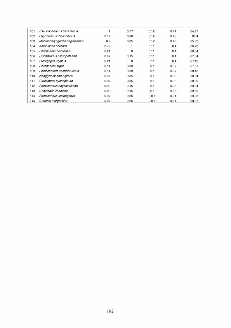
192
101 Pseudocheilinus hexataenia 1 0.77 0.12 0.44 84.97
102 Oxycheilinus rhodochrous 0.17 0.08 0.12 0.43 85.4
103 Macropharyngodon negrosensis 0.9 0.85 0.12 0.43 85.83
104 Amphiprion ocellaris 0.79 1 0.11 0.4 86.23
105 Halichoeres binotopsis 0.21 0 0.11 0.4 86.64
106 Dischistodus prosopotaenia 0.07 0.15 0.11 0.4 87.04
107 Pteragogus cryptus 0.21 0 0.11 0.4 87.43
108 Halichoeres argus 0.14 0.08 0.1 0.37 87.81
109 Pomacanthus semicirculatus 0.14 0.08 0.1 0.37 88.18
110 Neoglyphidodon nigroris 0.97 0.85 0.1 0.36 88.54
111 Cirrhilabrus cyanopleura 0.97 0.85 0.1 0.36 88.89
112 Pomacentrus nagasakiensis 0.03 0.15 0.1 0.35 89.24
113 Chaetodon lineolatus 0.03 0.15 0.1 0.35 89.59
114 Pomacentrus lepidogenys 0.97 0.85 0.09 0.34 89.93
115 Chromis margaritifer 0.97 0.85 0.09 0.34 90.27