Chapter 12:

Repetition and Reversibility in Evolution:

Theoretical Population Genetics1

Jean Gayon∗ and Maël Montévil†

∗ Université Paris I Panthéon-Sorbonne

† Université Paris 7 Diderot

Abstract

Repetitiveness and reversibility have long been considered as characteristic

features of scientific knowledge. In theoretical population genetics, repetitiveness is

illustrated by a number of genetic equilibria realized under specific conditions. Since

these equilibria are maintained despite a continual flux of changes in the course of

generations (reshuffling of genes, reproduction…), it can legitimately be said that

population genetics reveals important properties of invariance through transformation.

Time-reversibility is a more controversial subject. Here, the parallel with classical

mechanics is much weaker. Time-reversibility is unquestionable in some stochastic

models, but at the cost of a special, probabilistic concept of reversibility. But it does not

seem to be a property of the most basic deterministic models describing the dynamics

of evolutionary change at the level of populations and genes. Furthermore, various

meanings of ‗reversibility‘ are distinguished. In particular, time-reversibility should not

be confused with retrodictability.

1. Introduction

Evolutionary biologists commonly assume that ―evolution is unique and

irreversible‖. In contemporary literature, this claim is often closely related to the claim

that evolution is historically contingent from top to bottom with no laws and no genuine

theories. Although the authors share John Beatty‘s assertion that all (or almost all)

biological generalizations are ultimately historically contingent2, they believe that the

phrase ―evolution is unique and irreversible‖ is far too general and too vague to be

plausible. In reality, contemporary biology offers significant examples of repetition,

1To appear as: J. Gayon and M. Montévil, Repetition and Reversibility in Evolution: Theoretical

Population Genetics. In Time in nature and the nature of time (edited by C. Bouton and P. Huneman),

Springer. 2 On the ‗historical turn‘, see also Williams 1992, and Griffiths 1996. For a criticism of Beatty

1995, see Sober 1997.

invariance, and reversibility, both at the theoretical and the experimental level. Such

examples may help to get out of the too-narrow alternative between ―historical

contingency‖ and ―lawfulness‖ in biology, and particularly in evolutionary biology. In

a sense, this alternative suffers from its excessive philosophical radicalness. The issues

of repeatability vs. non-repeatability and reversibility vs. irreversibility of evolutionary

phenomena offer a useful tool to make the debate more nuanced. It may be the case that

repeatability and reversibility in evolution are marginal; nevertheless there are clear

cases, both at the theoretical and the experimental level. The present paper will

concentrate exclusively on theoretical population genetics.3

What exactly do the terms ―repeatability‖ and ―reversibility‖ mean? The

definition is a delicate issue here, especially for the second notion. Does reversibility in

evolution mean that an evolving entity (e.g. a population or a species) can return to a

previous state (whatever the trajectory), or that the reverse trajectory should be strictly

symmetrical with the direct trajectory? In his papers on the irreversibility of evolution,

the Belgian Palaeontologist Louis Dollo was particularly concerned by this latter sense

of ―reversibility‖: ―In order for [evolution] to be reversible, we would have to admit the

intervention of causes exactly inverse to those which gave rise to the individual

variations which were the source of the first transformation and also to their fixation in

an exactly inverse order‖ (Dollo 1913, quoted in Gould 1970, p. 199). Another

difficulty arises from the technical notions of reversibility used in mathematics and

physics. Do these notions apply to evolutionary biology? One of the main objectives of

this chapter is to clarify the varying meanings of repetition and reversibility applicable

to evolution. Repetition is a simpler matter, but this notion also involves a certain

amount of ambiguity. Indeed, the two notions of repetition and reversibility should not

be conflated as George Gaylord Simpson did when he commented on Dollo: ―…

evolution is a special case of the fact that history does not repeat itself. The fossil

record and the evolutionary sequences that it illustrates are historical in nature, and

history is inherently irreversible‖ (Simpson 1964, p. 196; quoted in Gould 1970, p. 208-

209). Simpson‘s statement seems a little too obvious. Although evolutionary

reversibility is most often related to the kind of repetition that is so important for living

beings—reproduction—repetition and reversibility should be clearly distinguished from

one another.

When Louis Dollo introduced his famous ―law of irreversibility in evolution‖, he

defined it in the following terms: ―… an organism cannot return, even partially, to a

former state already realized in the series of its ancestors.‖ (Dollo 1893, translated by

Gould 1970, p. 211). As suggested by this formula, Dollo was interested in the problem

of reversibility be it at the level of the organism or at least of a complex organ.

Furthermore, as a palaeontologist, he conceived his ―law‖ as applying to a large

temporal scale (macroevolution in modern terms). Dollo did not deny that reversion

could occur at more elementary levels. Moreover, neither genetics nor even less

3 Another paper, devoted to experimental biology, will be published separately

population genetics, existed when Dollo proposed his law of irreversibility in evolution.

Therefore, and in view of present knowledge, it seems appropriate to reassess the

problems of invariance and reversibility at a microevolutionary level.

Repetitiveness and reversibility in evolution can be assessed at two different

levels, empirical and theoretical. At an empirical level, living objects exhibit properties

of invariance that are crucial for evolutionary change. Current examples of invariance

include gene replication and constancy of the number of chromosomes in the process of

cell reproduction; and reproduction and alternate generations at organism level. In such

cases, invariance is not absolute, indeed the replication of genetic material is not always

perfect; correlatively, hereditary material exhibits an ability to change (genic mutations,

recombination, chromosomal accidents…). Similarly, reproduction can encounter

accidents (e.g. developmental anomalies), and exists under various modes (e.g. asexual

vs. sexual reproduction, diverse schemas of alternate generations). Replication and

reproduction are very general properties of living beings, and provide a basis for

evolutionary models. They objectively exist throughout the living world. Of course,

they result from a historical process, and for that reason, they cannot be thought of in

terms of ―laws of nature‖ in the sense of universal statements of unlimited scope,

applying everywhere and at any time in the universe. One of us advocates the use of the

concept of constraints in order to discuss limited invariance in the context of biological

historicity (Longo and Montévil 2014, Montévil and Mossio 2015).

Population geneticists also share an intuitive notion of reversibility. Some

biological processes make the return of a population to a previous state possible.

Obvious examples include reverse mutation, especially if repeated; backwards selection

(i.e. inverted selection coefficients); and chance (random drift). What ―reversibility‖

precisely means in these examples is open to question, however the idea that

populations can return to a previous state is perfectly plausible, given the nature of the

basic biological processes involved in genetic evolution. There is another manner of

formulating the intuitive notion of reversible evolution, which is more precise and

better adapted to present genetic knowledge, namely: ―for a given individual, consider

the set of all its possible genetic states. One can move from one state to another thanks

to the ordinary sources of genetic change (substitution of nucleotides, deletion,

insertion, recombination, etc.). It is obvious that any sequence of states E1, E2… Ei… Ek

that an individual can follow can also be followed in the reverse direction.‖ (Goux

1979, p. 568, our translation).

These intuitive notions of repetitiveness and reversibility come prior to the

construction of models in population genetics. They should be carefully distinguished

from the properties discovered through the development of theoretical models

describing the genetic evolution of populations. At that theoretical level, non-trivial

notions of repetitiveness and reversibility occur; they result from modelling itself.

Section 2 shows how population genetics models satisfies a characteristic feature of

scientific knowledge currently found in the physical sciences, namely the discovery of

formal properties of invariance through transformation. The next section examines

whether theoretical genetics has also the capacity of discovering properties of

reversibility or not. This is a more difficult issue. After defining several possible

meanings of reversibility, section 3 shows that time reversibility in the mathematical

sense is illustrated by some stochastic models, whereas basic deterministic models do

not exhibit the property of time-reversibility. The concluding section raises serious

doubts about the traditional comparison made between classical mechanics and the

deterministic models of population genetics.

2. Repetitiveness in theoretical population genetics

Jean-Michel Goux observes that the source of a number of equilibria in

population genetics is the endless repetitiveness of the life cycle (1979, p. 567). We

will here freely expand on this proposal. In spite of its sophisticated use in

mathematics, the notion of invariance under transformation can be defined in a simple

and general way, and can be applied to many different areas of knowledge, not only in

mathematics and theoretical physics. For a given class of objects, an invariant is a

property that remains unchanged when a specified type of transformation is applied to

the objects. This concept is especially fruitful when the objects and their relations are

described by mathematical formulae; in such cases, a precise sense can be given to

what is said to be invariant.

One of the most famous examples of invariance to transformation in physics is

the Galilean transformation. In its traditional formulation in classical mechanics,

Galileo‘s principle of invariance (also called Galileo‘s principle of relativity) states that

the laws of motion are the same in all inertial frames. Based on the postulate of

absolute time and absolute metric of space, this principle makes the transformation of

spatial and temporal coordinates from one inertial referential system to another

possible. For instance, if the speed of material point in S is v, its speed in S’ will be4:

Vx’ i = dx’/dt = d(x-vt)/dt = vx - v

Invariants through transformation may be of many kinds. In classical and

relativist mechanics they are relative to motion. However they can also be relative to

structures (i.e. the composition of a particular class of objects). This section considers

the case of invariance relative to the genetic structure of a population in specified

conditions. Some classic examples of genetic equilibria are given below, which all

belong to what could be called evolutionary statics, as opposed to evolutionary

dynamics. Time-reversibility is also an extreme case of invariance through

transformation. This notion will be considered in section 3, devoted to evolutionary

dynamics in population genetics.

The Hardy and Weinberg equilibrium is certainly the best-known example of a

structural invariant. Consider a single locus with two alleles A and a with frequencies p

4 In the simple case where the spatial coordinates are chosen so that the origins O and O’ of the

two referential systems coincide for space and time. Then the three axes move along a line Ox.

and q (with p + q = 1)5. The Hardy and Weinberg law states that, irrespective of the

initial gene frequencies and the initial genotype frequencies, if [1] all crosses occur

within the same generation (no overlapping generations), if there is [2] no selection, [3]

no migration, [4] no mutation, if [5] mating is random, and if [6] if the population size

N is big enough to consider that 1/N ≈ 0, then the genotypic frequencies are constant

and depend only on the gene frequency of the initial generation (for a precise

formulation of these conditions, see Jacquard 1971, p. 48-58, and Hartl, 1980, pp. 93-

94). Under such conditions, the expected genotypic ratios are AA : p2 ; Aa : 2pq ;

aa : q2. In a discrete-generation population, the population immediately achieves these

proportions from the first generation of mating, and the expected ratios remain constant

as long as the six conditions mentioned are satisfied. The Hardy and Weinberg [HW]

law derives its name from the British mathematician G. H. Hardy6 (1877-1947) and the

German physician and obstetrician Wilhelm Weinberg (1835-1937), who

independently and simultaneously demonstrated it in 1908 (Hardy 1908; Weinberg

1908). Some authors call it a ‗principle‘ (Crow and Kimura 1970). But it is more

accurately characterized as a theorem, because it can be demonstrated on the mere basis

of the Mendelian law of segregation and the six conditions stated above. It is also

commonly referred to as ―the Hardy-Weinberg equilibrium‖, where ―equilibrium

[refers] to the fact that there is no tendency for the variation caused by the co-existence

of different genotypes to disappear‖ (Edwards 1977, p. 7). The reason why this law is

so important is that it purely expresses the effect of Mendelian inheritance in the

absence of any factor able to change the genetic frequencies (i.e. gene frequencies and

genotypic frequencies)7. As Edwards puts it, ―this ability to maintain genetic variation

is one of the most important aspects of Mendelian genetics‖ (ibid.). The constancy of

genetic frequencies under Mendelian inheritance provides a reference model for

describing the effects of evolutionary ―forces‖, especially mutation, migration,

selection, population size, inbreeding, and the mating system (homogamy vs.

heterogamy), which may modify the genotypic structure of the population8. Returning

to the problem of repetitiveness, the HW equilibrium is typically an invariant under

transformation, because it identifies something (the distribution of gene and genotypic

frequencies) that persists in spite of the indefinite reshuffling of the alleles that meiosis

5 In genetics, a locus is a particular position on a chromosome, occupied by a gene, which can

itself exist under several alternative versions, named ‗alleles‘. The Hardy-Weinberg equilibrium applies

to sexually reproducing and diploid species, where all chromosomes (except fot the sexual chromosome)

exist in pairs. 6 Godfrey Harold Hardy did not use his first Christian name with his friends, but rather ‗Harold‘

(Anthony Edwards, personal communication). 7 This is why Sober calls the HW principle the "zero force law of population genetics" (Sober

1984). Gayon (1998) qualifies the Hardy-Weinberg equilibrium as an equivalent of the principle of

inertia in classical mechanics (see however the conclusion of the present paper), which challenges this

view. 8 Some of these factors modify both the gene and the genotypic composition of the population.

Others (homogamy) modify only the genotypic structure.

dissociates at each generation. Of course, the HW law is an idealization, because no

real population ever strictly satisfies the conditions that permit its derivation.

Another classic example of structural invariance under transformation in

population genetics is ―Wright‘s principle‖, also called ―Wright‘s law of equilibrium‖.

This gives the frequency distribution of genotypes in an infinite population, for a

diallelic locus9:

(p2+Fpq) + 2pq(1-F) + (q

2+Fpq) = 1

where F is the coefficient of inbreeding. This law expresses the zygotic

proportions10

expected in a population with a certain amount of inbreeding, in other

words a population where mates are more closely related than if they were chosen at

random. The Hardy-Weinberg equilibrium is in fact a particular case of Wright‘s

equilibrium, corresponding to F=0. Therefore, Wright‘s law of equilibrium takes into

account one of the major causes of departure from the HW equilibrium (the other one

being assortative mating). The F coefficient may of course change. Nevertheless,

Wright‘s formula states that for a given F, and if no other factor is allowed to modify

the genotypic frequencies, the genetic structure of the population is invariant from

generation to generation. Apart from the Hardy and Weinberg law and Fisher‘s 1918

paper on the correlation between relatives under Mendelian Inheritance (Fisher 1918),

this is one of the oldest results in theoretical population genetics. It has been

demonstrated several times, and improved and generalized (multi-allelism) since

Wright‘s original paper in 1921 (Wright 1921; Malécot 1948; Li 1955).

As said earlier, the Hardy and Weinberg equilibrium is established as early as the

first generation of crossing (the first zygotes made from the previous generation). But

this is true only if generations do not overlap (see above: condition 1). If generations

overlap, it takes more time for the HW equilibrium (as well as Wright‘s equilibrium) to

be established, but the population does converge towards this equilibrium. Therefore,

the equilibrium does not emerge immediately, as in the discrete case, but gradually, as

what could be described as a ―trend‖.

This notion of ―trend‖, which is very ubiquitous in theoretical population

genetics, leads to an important remark about equilibria in this discipline. The search for

equilibria is an important part of theoretical population genetics. Developing an idea

suggested by J. B. S. Haldane, Crow and Kimura speak of ―evolutionary statics‖, as

opposed to ―the dynamics of evolution‖. In a paper entitled ―The Statics of Evolution‖,

Haldane (1954) declared that, in spite of evolution being a ―dynamical process‖, a good

deal of it is better understood in terms of ―statics‖. Haldane stated that the reason for

this was that evolution is usually an extremely slow process, which may, nevertheless,

rely upon strong forces (esp. selection). Whence the idea that an important part of

evolutionary processes should be thought of in terms of ―approximate equilibria‖

resulting from a balance of ‗forces‘ that quite often conflict with each other (e.g.

9 Diallelic locus : refers to a locus with two alleles.

10 A zygote is a diploid cell (two stocks of chromosomes) resulting from the fusion of two haploid

cells (spermatozoon and ovum), which have only one stock of chromosomes.

various kinds of selection, selection and migration, selection and mutation, etc.), and

that result in the persistence genetic polymorphism. The ‗statics‘ of evolution is indeed

one of the most spectacular parts of theoretical population genetics. Quite often, the

results are simple, elegant and easily found, in contrast to the difficulty associated with

the mathematical treatment of the ‗dynamics‘ (which will be evoked in the next section,

when coming to ‗reversibility‘). For this reason, equilibrium formulae play an

important role in the elementary teaching of population genetics.

In their Introduction to Population Genetics Theory (1970), Crow and Kimura

devote an entire chapter to ―Populations in approximate equilibrium‖ (Chap. 6). They

examine an impressive list of factors maintaining gene frequency equilibria. All these

factors ―depend on some kind of balance between opposing forces‖ (Crow and Kimura

1970, p. 256). A partial list of the types of such equilibria is given below (from Crow

and Kimura 1970, p. 256-196). Quite often, the models obtained are simple. Illustrative

examples are given for the first two categories in the list.

- Equilibrium between selection and mutation. For instance, in the case of a single

locus with complete dominance where the recessive homozygous-mutant

genotype is disadvantaged, and where mating is random, the equilibrium is

reached when 𝑞 = 𝑢

𝑠

with q: frequency of the mutant gene; u: mutation rate; s: selection coefficient.

- Equilibrium under mutation pressure (infinite population, no random drift). For

instance, in the simple case of a two-way recurrent mutation, the equilibrium is

reached when 𝑝 =𝑣

𝑢+𝑣, with u and v being the mutation rates from and to allele A,

and p the frequency of A.

- Equilibrium between migration and random drift.

- Equilibrium under selection: stabilizing selection (selection directed towards the

elimination of deviants)11

, advantage to the heterozygote12

, frequency dependent

selection13

, disruptive selection (selection in varying directions), multi-niche

polymorphism…

- Selective models accounting for the constancy of sex ratio (most often 1:1 at the

age of reproduction).

All these equilibria—and this list is not exhaustive—isolate an invariant under

transformation. For instance, the model for a two-way recurrent mutation tells us how

the genetic structure of a population (both gene frequencies and genotypic frequencies)

11

This kind of selection favours the mean type. 12

This kind of selection favours the individuals with genotype Aa. A classic example is the better

resistance to malaria of individuals who are heterozygotes for the gene responsible for sickle cell anemia.

Double recessives aa suffer from severe anemia and most often die at an early age; double dominant AA

are much less resistant to malaria than heterozygotes Aa in areas infected by Plamodium falciparum. See

Figure 7. 13

In this kind of selection, the selective values of the genotypes depend on the allelic frequencies.

This results in an intermediate equilibrium.

is preserved as long as the same conditions hold. In spite of the endless reshuffling of

genes and of changes recurrently caused by two mutation pressures, an equilibrium is

attained. Despite the obvious complexity and historicity of evolutionary phenomena,

equilibrium models reveal invariant relations between parameters (gene and genotypic

frequencies, mutation rates, selection rates, etc.) under idealized conditions.

The discovery of formal properties of invariance through transformation is an

important component of scientific knowledge, whether in biology, physics or

economics. In his Models of Discovery, Herbert Simon once wrote that ―the notion of

invariance under transformation as a necessary condition for a ‗real‘ property of a

physical system has provided a leading motivation for the development of relativistic

mechanics and other branches of physics‖ (Simon 1977, p. 79, n. 8). We should not be

surprised to find such invariants in evolutionary theory. As previously stated,

repetitiveness is a massive empirical property of living beings: repetitiveness of life

cycles, repetitiveness of cellular reproduction, repetitiveness of gene replication, and

also repetitiveness of occasional phenomena such as recurrent mutation at population

level. Given that repetitive phenomena are so widely observed at an elementary level, it

is reasonable to expect that more formal invariants emerge when population genetics

extrapolates from these empirical cases of repetitiveness to the behaviour of

populations. As suggested in the introduction, the huge degree of historicity and

contingency in evolution should not dismiss a certain amount of lawfulness, at least at

the microevolutionary level.

3. Time-reversibility

Time reversibility is a less obvious notion than invariance through

transformation, for two reasons. First, it refers to problems that may become highly

technical, and counter-intuitive in terms of their mathematical treatment. Secondly,

evolutionary biologists use different notions of reversibility, and very often they do this

unconsciously. Discussing time reversibility with several population geneticists, we

have been struck by the combination of spontaneous certainty and doubt manifested in

their spontaneous reactions to this subject. One of the most common reactions was:

―yes, obviously, the deterministic models (esp. models of selection) are reversible, but,

if random drift is taken into account, the opposite is true… Markovian processes are

deprived of memory…‖. Another rarer response was: ―Most probably, the equations

describing the effect of deterministic processes do not describe reversible processes, but

it seems evident that there is a large amount of reversibility in the models describing

stochastic events‖. Such contradictory statements, made by some renowned population

geneticists, triggered our curiosity. But the most common thought was of the following

type: ―obviously‖ the biological processes involved in the evolution of a population

may ―in principle‖ cause the return of the population to a previous state. For instance, if

a mutant allele gets fixed, there is always the possibility that a reverse mutation will

trigger a reverse evolution (through the accumulation of such mutations, or appropriate

selective pressure, or random drift). Similarly, if the hierarchy of selective pressures is

inverted, then reverse evolution will follow14

. In fact, it seems that population

geneticists, although excited by the problem, do not have a clear and articulate position.

They use the word to have various meanings. This section intends to clarify the several

possible meanings of ‗reversibility‘ with respect to population genetics.

Three different senses of ‗reversibility‘ can be found in the current—mainly

mathematical and physical—scientific literature. After giving definitions for these, the

level of their applicability to population genetics will be considered and the less

conventional and specifically biological meanings of ‗reversibility‘ among population

geneticists will be discussed.

3.1 Three senses of ‘reversibility’

To correctly treat reversibility as an operational concept in mathematics, physics

and other exact sciences, would require a more formal and detailed analysis. The

remarks that follow will only sketch out some distinctions that may help clarify the

problem of reversibility in population genetics15

.

3.1.1 Retrodictability

In classical mechanics, prediction and retrodiction are symmetrical: knowing the

law(s) governing the development of a certain phenomenon through time and the state

of the system at a given time t, it is possible to infer the state of the system at any other

time, past or future. For instance, given Kepler‘s laws for the motion of the planets in

the solar system, and given appropriate information about the state of a planet a time t

(that is the position and instantaneous speed of the planet considered, as well as of other

planets that interact with it), the position and speed of this planet at any past or future

time can be inferred. What is required for retrodictability is the possibility of deriving a

backward equation from the forward equation that describes the past trajectory as

precisely as the forward equation describes the normal motion. For such an inference,

the astronomer‘s theoretical framework does not need to be perfect. It may have, and

certainly has its own limits (for instance Poincaré‘s three bodies problem). We just

assume a certain more or less sophisticated theoretical system, describing a

deterministic process. If the process is deterministic, prediction and retrodiction are

expected to be equally possible; note also that, in discrete time, retrodictibility may

sometimes be impossible for deterministic systems (see Appendix 1). Retrodictability is

often associated and identified with time reversibility in the mathematical sense (see

14

Here is an example : in the 19th Century, the proliferation of melanic forms of moths in

industrial regions resulted from the darkening of the bark of trees by soot: the dark forms were better

protected against predation by birds. With desindustrialization, light forms replaced dark forms. This is a

typical case of inversion of selective pressure. 15

We are very much indebted to Jean-Philippe Gayon, Anthony Edwards, Pierre-Henri Gouyon,

and Michel Veuille, for their helpful interaction on this subject.

below, [2]), and the two notions may indeed be closely related in particular cases. But

as will be seen shortly, they are distinct. Because of the confusions resulting from

equating retrodictability and reversibility, speaking of retrodiction (inference to the

past) as a case of ‗reversibility‘ should definitely be avoided. Although not common

usage, the rest of this paper will repeatedly distinguish ‗time-reversibility‘ (reversibility

sensu stricto) and retrodictability.

3.1.2 Time reversibility in the conventional ‘mathematical’ sense

The notion of time-reversibility is based on a comparison between normal

trajectories and trajectories after time reversal, that is to say where the past becomes the

future and the future becomes the past. Reversibility occurs when these two trajectories

follow the same law. Conversely, when the dynamics are irreversible, the law provides

an orientation to time (the ‗arrow of time‘). The question of time-reversibility in this

sense is commonly discussed in theoretical physics, see for example chapter 7 and 8.

From a technical point of view, a time-reversible process is such that the

equations describing its dynamics are invariant if the sign of time is reversed. In other

words, if ‗-t‘ is substituted for ‗t‘, the law(s) governing the phenomenon is unaffected.

In the case of classical mechanics, this will usually be checked by looking at the second

order derivative of the equation describing the trajectory of the system. Consider for

instance Galileo‘s law of falling bodies, which states that the distance x travelled by a

free-falling body is directly proportional to the square of the time t for which it falls:

x= 1/2gt2. The first order derivative, dx/dt = gt gives the speed. The second order

derivative, d2x/dt

2 =

g gives the acceleration, which is the key element from a dynamic

point of view. It is easily seen that substituting –t for t in this second order derivative

does not change anything. The same ‗law‘ holds in both time-directions. This means

that, if a ball is thrown up, the law governing the motion of the rising ball is identical to

the law that describes the motion of the falling ball (not similar, but identical). The

direction of the trajectory will be inverted, of course, and the speed will diminish

instead of increasing, but the rate of the decrease will be strictly the same as the rate of

the increase: the dynamics governing the process is the same. This is exactly what the

second order derivative says: since t exists only as a square number in d2x/dt

2 =

g, this

equation is not affected by an inversion of time. The transition from t to t+1 and the

transition from t+1 to t are said to follow the same ‗law‘. Indeed, this insensitivity can

be demonstrated for both a discretized formulation of Galileo‘s law (where the

evolution of the system is described at successive discrete steps, t, t+1, etc.) and for

continuous time (that is using a differential equation). In this precise sense, time

reversibility is traditionally seen as an almost universal property of the laws of classical

mechanics. In this respect, the best examples of time-reversibility (T-symmetry) are to

be found in the fundamental laws of mechanics, which give the basic dynamics

underlying mechanical processes. Newton‘s law expressing the relationship between

force and acceleration (F = ma) would certainly be a better example than Galileo‘s law,

an empirical law describing a trajectory rather than genuine dynamics. It is easy to

understand that d2x/dt

2 = F(x)/m holds also after time reversal. With Newton‘s law,

there is no need to be concerned with the counter-intuitive representations associated

with a falling body governed by the same law both when it falls and when it is ‗thrown

up‘, or ‗reverts‘ (when, how, what initial conditions, etc.—all elements that are unclear

in the example). It should be noted, however, that Newton‘s law, F = ma, is time-

reversible if and only if F is symmetrical by time-reversal (see Appendix 1.1 for a more

formal definition), for example when F depends only on x. This is the case for all

classical fundamental forces, gravitation and electromagnetism. However, in other

cases such as friction, where F = –fdx/dt (where f is the friction coefficient), the law is

no longer reversible.

The relation between reversibility and retrodictability is a delicate problem. The

two notions may be closely related in particular cases. For instance, Galileo‘s law

discussed above, allows for both retrodictability and reversibility. Knowing the position

and the speed of a material point at any instant enables the prediction of the future and

of the past position and speed of this material point at any time (within the limits of the

actual trajectory). But Galileo‘s law also satisfies the condition of reversibility: it

describes a transformation in both possible directions. However, the two notions are not

necessarily associated. Consider the case of discrete time equations, which are

particularly important in population genetics. The function g allowing a ‗prediction of

the past‘ may be totally different from the function that describes how the system

passes from t to t+1. Now consider a recurrence equation of the form p(t+1) = g[p(t)].

Reversibility means:

p(t+1) = g[p(t)] → p(t) = g[p(t+1)] [1]

with p designating some function of time, and g the function defining the

dynamic of p (i.e. what future state follows from the current state).

This formula means that the transition from t to t + 1 and the transition from t + 1

to t follow the same law.

We can similarly express the idea of retrodictability:

p(t + 1) = g[p(t)] → p(t) = h[p(t + 1)] [2]

where h is a function derived from the recurrence formula, which allows

‗retrodiction‘. The functions h and g may be totally different. For more precise

definitions of reversibility and retrodictability, see Appendix 1.1 (continuous time) and

1.2 (discrete time).

Finally, there is another, important reason why retrodictability and reversibility

should not be confused. So far, time-reversibility has been discussed only in the context

of deterministic processes. However, time-reversibility can also be a property of

stochastic processes: if the stochastic properties of a process depend on the direction of

time, this process is said to be irreversible; if they are the same for either direction of

time, the process is called reversible. Let X(t) be a stochastic process, and τ a time

increment. A standard definition of time-reversibility for a stochastic process is:

―A stochastic process X(t) is reversible if (X(t1), X(t2), …, X(tn)) has the same

distribution as (X(τ-t1), X(τ-t2), …, X(τ-tn)) for all t1, t2,…, tn‖ (Kelly 2011, p. 5) [3]

This definition means that the joint probabilities of the forward and reverse state

sequences are the same for all sets of time increments. This notion can be applied to a

Markovian process (i.e. in a state of equilibrium), that is to say a random process that

undergoes transition from one state to another with no memory of the past. In a state of

equilibrium, the condition for reversibility is:

ΠiPi,j = ΠjPj,i [4]

where Pi,j is the transition probability from state i to state j, and ΠiPi,j the

probability flux from state i to state j. Πi is the proportion of the population in state i.

This formula does not explicitly include the time parameter t, but time is implicit

through the notion of transition.

This statistical notion of reversibility has been fruitfully applied to a number of

subjects, such as queuing networks, migration processes, clustering processes (esp. the

equilibrium distribution polymerization process), and also population genetics, where

Markovian processes are tremendously important for the treatment of random genetic

drift (Kelly 2011). In contrast with reversibility in deterministic systems, stochastic

time-reversibility is hardly compatible with retrodictability. Retrodictability is

ordinarily understood as the possibility to reconstitute the actual trajectory that led to

the present state, and is strongly associated with determinism, or at least to the idea of a

causal sequence that has driven the trajectory. The notion of retrodictability could

perhaps be extended to stochastic processes, but this is not the usual way of thinking

about it. Furthermore, this would probably be a strange way of thinking in the case of

time-reversible stochastic evolution, because stochastic reversibility is a typical case of

an invariant and stationary state.

To sum up, although simple in principle (insensitivity of a given law to time

reversal), the ‗mathematical‘ notion of reversibility is delicate. It is not synonymous

with retrodictability, and it does not only apply in deterministic situations.

3.1.3 ‘Physical’ or ‘thermodynamic’ notion of reversibility

The ‗physical‘ notion of reversibility is closely related to thermodynamics. Both

denominations are unsatisfying, because the former arbitrarily restricts the notion of the

‗physical‘16

, while in fact the latter extends beyond thermodynamics. ‗Physical‘

reversibility means that a physical system can spontaneously return to a prior physical

state. A classical (although not perfect) example is given by a spring, which returns to

its prior state after being elongated. By contrast, we do not expect that a broken glass

will spontaneously find again its original shape. This is quite different from the

property of insensitivity to time reversal. Consider a glass that breaks into pieces after

falling. The glass would not be expected to spontaneously reacquire its original,

16

As seen in the previous paragraph, the insensitivity of the laws of classical mechanics to an

inversion of time is as ‗physical‘ as thermodynamic irreversibility is ‗physical‘.

ordered structure. Another example is that of a marble in a bowl. If there were

absolutely no friction, the ball could go up and down the sides of the bowl indefinitely.

But there is always some degree of friction. Therefore the oscillations of the marble

will steadily decrease in amplitude, and in the absence of an external force, the marble

will finally stop moving. These two examples (broken glass and rolling ball) illustrate

the notion of physical irreversibility.

The traditional physical notion of reversibility is closely associated with

thermodynamics: reversible evolution of a system is a type of evolution where no

entropy is produced. Conversely, the greater the entropy, the more irreversible the

transformation of the system. In a closed system, entropy is a quantity that can only

increase. A precise definition of what this quantity precisely means is not needed here,

nor are the classical debates on entropy as a property of macroscopic systems, as

opposed to the reversible phenomena that underlie irreversible behaviour at a

macroscopic level. For the needs of the present paper, suffice to retain that the physical

(or thermodynamic) notions of reversibility and irreversibility are closely related to

those of conservative vs. dissipative systems. A conservative system allows for

reversible transformation; a dissipative system implies a dissipation of energy (e.g.

diffusion of heat and friction), which renders the transformation irreversible, see

chapter 5 for a short discussion on the origin of irreversibility in thermodynamics.

From a thermodynamic point of view, biological phenomena are widely thought

to be far-from-equilibrium processes: they maintain a relatively low entropy thanks to

flows of energy and matter. Because they produce entropy, they are irreversible from

the thermodynamic perspective. However, this aspect concerns energy and energy

dispersal in a space of positions and momenta (measured in physical units), which is

different from the space of gene populations that we discuss in this paper (gene

frequencies are not measured in physical units). As a result, thermodynamic

irreversibility is analytically independent from the question of the intrinsic time-

reversibility or time-irreversibility of population genetics models.

3.2 Retrodictability and reversibility in theoretical population genetics

The various notions of reversibility mentioned in the previous paragraph will now

be applied to theoretical population biology. No attempt is made here to be exhaustive.

The present analysis will be limited to a few typical cases. Stochastic and deterministic

processes will be successively examined, and a few remarks will be made about cases

of ‗reversibility‘ in population genetics that do not fit with the proposed categorization,

cases where the notion of evolutionary reversibility relies on specific biological

processes.

3.2.1 Stochastic processes

Stochastic processes probably offer the best and most spectacular cases of time-

reversibility in the strictest mathematical sense, that is to say insensitivity of a given

model to reversal of time. This is most explicit in G. A. Watterson‘s two articles on

―Reversibility and the Age of an Allele‖ (1976 and 1977). These papers consider the

probability distribution of the age of a mutant allele, whose present frequency is

known. The ‗age of an allele‘ is defined as the time that has elapsed between the

introduction of the allele by mutation and the present. In the first paper (1976), the

author assumes that there is no mutation and no selection. The model is set in discrete

time, and admits that there is an infinite number of possible neutral alleles and thus

discuss genetic drift. The method consists in taking y, the present frequency of the

mutant gene, as ―the initial state of a stochastic process, and studying how long

diffusion would take to reach state x (or state 0) for the first time‖ (x being the

frequency at a time t units prior to the present). Watterson is very explicit about the role

of time-reversibility in his model, the general spirit of which is presented in the

following terms:

―This interpretation seems surprising on two counts: first, because it means that

the published results are simply moment of extinction times for diffusions, and

second, there are stochastic processes for which this reversibility is valid, that is,

processes whose behaviour looking into the past is statistically identical with their

future behaviour.‖ (Watterson 1976, p. 240)

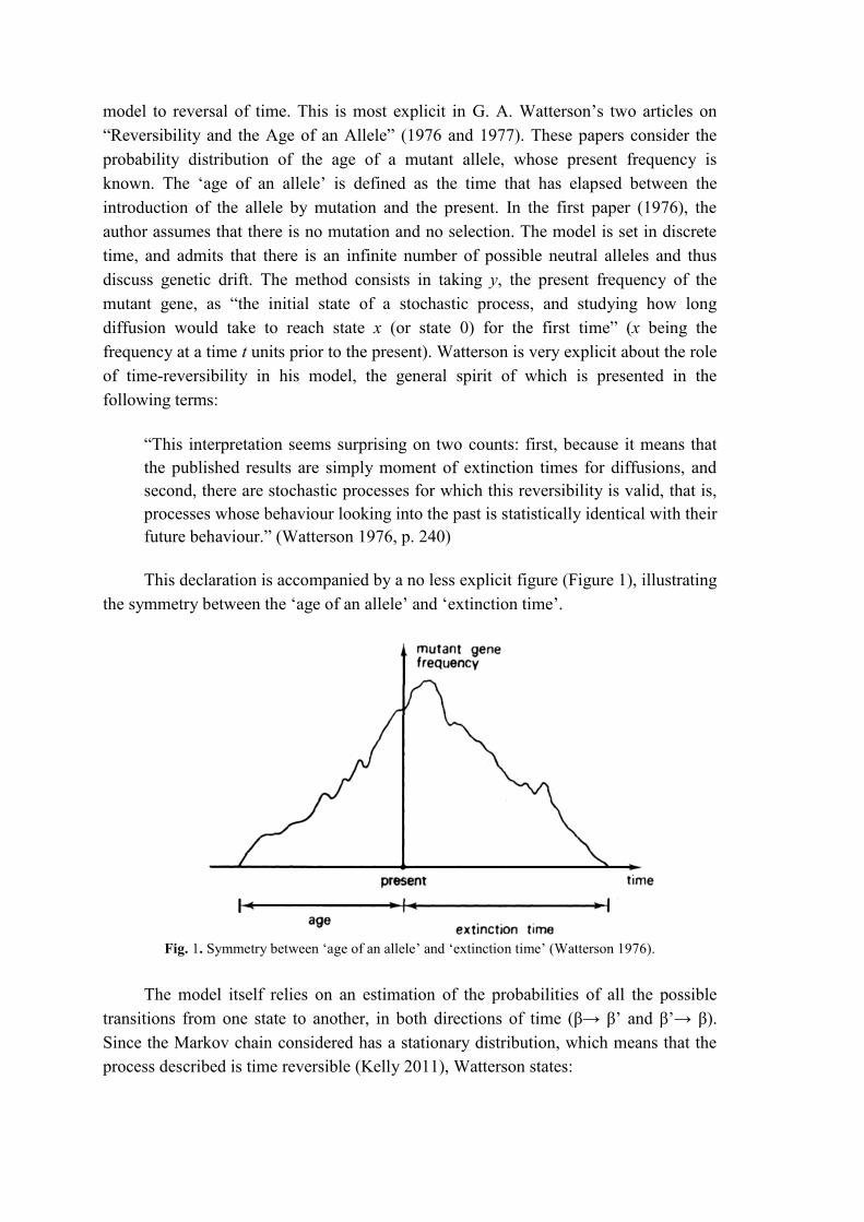
This declaration is accompanied by a no less explicit figure (Figure 1), illustrating

the symmetry between the ‗age of an allele‘ and ‗extinction time‘.

Fig. 1. Symmetry between ‗age of an allele‘ and ‗extinction time‘ (Watterson 1976).

The model itself relies on an estimation of the probabilities of all the possible

transitions from one state to another, in both directions of time (β→ β‘ and β‘→ β).

Since the Markov chain considered has a stationary distribution, which means that the

process described is time reversible (Kelly 2011), Watterson states:

―The consequence of reversibility for the stationary configuration process is that

we can discuss its past evolution with equal ease as its future evolution; β(t), β(t-

1), β(t-2), β(t-3),… have the same joint [sic. ‘probability‘ ?] as have β(t), β(t+1),

β(t+2), β(t+3),…ˮ (Watterson 1976, p. 243).

The main conclusion of the paper is that ―…the age distribution {Pi(a)} for an

allele now represented by i genes in the population is the same as the extinction time

distribution for such an allele. Moreover, {Pi(a)} is independent of the frequencies of

the other alleles in the population.‖ (Ibid., p. 246). This is a remarkable result,

illustrating the usefulness of time-reversibility for the elaboration of models in

population genetics: ―By reversibility we mean that given the present state of a

stochastic process, the statistical properties of its future behaviour are the same as those

for its past history treated as a stochastic process with time running in the reverse

direction.‖ (Watterson 1977, p. 179) Watterson‘s notion of reversibility corresponds to

that defined in equations [3] and [4].

In the same spirit, time-reversibility has been extensively used in coalescent

theory, which is probably the major innovation in population genetics since the 1980s

(Kingman 2000). Coalescent theory is concerned with gene genealogies within species.

Relying on neutral mutations and the assumption of randomness of reproduction, its

basic idea is to estimate the average time at which several genes share their most recent

common ancestor. Time reversibility of the genealogical process is crucial in this case.

3.2.2 Deterministic processes

Population genetics theory is commonly divided into two main branches. The

first is stochastic theory, which focuses on the effect of random changes, especially

"random drift", in allelic and genotypic frequencies. The second focuses on

―deterministic‖ effects of factors such as mutation, migration, selection, and mating

system. The deterministic theory of population genetics ignores the random changes,

and is therefore less complete than the stochastic theory (Ewens 2012). In fact, all real

processes in nature include a stochastic aspect, not least because real populations are

finite and inescapably subject to random drift. Consequently, in the real world,

deterministic factors always interact with stochastic factors. Furthermore, when

population geneticists speak of the evolutionary factors in terms of ‗forces‘, it is only a

metaphor. Some philosophers defend that population genetics does not deal with

physical forces but with statistical effects (Walsh, Ariew, and Lewens 2002; Matthen

and Ariew 2009; Huneman 2013). Nevertheless, the notion of ‗deterministic‘ factors in

population genetics is acceptable in the sense of factors that have a directional effect,

and tend to push gene and genotypic frequencies in one direction, up, down, or

intermediate. Recurrent mutation, selection, migration and non-random mating are the

commonest cases of such deterministic factors. Just as forces in mechanics, they

produce either secular changes that result most often in states of equilibrium such as the

fixation of an allele at frequency 0 or 1 (e.g. one-way mutation pressure), or

maintenance of genetic frequencies at an intermediate value (e.g. two way recurrent

mutation pressure, or selection with advantage to the heterozygote). The importance of

these ―deterministic factors‖ led J. B. S. Haldane to say that population genetics—

especially the genetic theory of natural selection—is part of the ―mechanics of

evolution‖. This is indeed a tempting metaphor, which one of the authors has endorsed

in the past (Gayon 1998, Chap. 8). However, in view of the issue of the time-

reversibility of equations, we are inclined to significant reservation about this

metaphor. Thus, to what extent and in what sense are the equations describing the

dynamics of deterministic processes in population genetics ‗reversible‘?

3.2.2.1 Retrodictability

The issue of retrodictability will be considered first. Intuitively, if the existence of

deterministic models in population genetics is accepted, the answer seems obvious.

Richard Lewontin is particularly clear on this issue:

―It is usual for population geneticists, who claim that they are studying the

dynamics of evolution, to divide the kinds of models that they deal with in two

sorts. They talk about deterministic models and about stochastic models? What is

meant by deterministic models is that, given the initial conditions of the

population, which I will simply specify by X0 (although that will be some sort of

a vector of conditions of the population), and some set of parameters, then it is

possible to predict exactly the condition of the population at some other time, τ.‖

(Lewontin 1967, p. 81)

By ―some other time‖, Lewontin means any other time, past or future, as

explicited a few pages later in the famous 1967 paper on ―historicity in evolution‖: ―If I

just give you one history of a deterministic population because it is deterministic I can

say everything about its past‖ (Lewontin 1967, p. 87). This is exactly what

retrodictability means.

Population genetics textbooks are replete with deterministic models describing

the effects on gene and/or genotypic frequencies, of factors such as recurrent mutation,

migration, selection, and mating system. In these models, evolutionary time can be

treated in two ways, discrete or continuous17

. With discrete time, the time-unit is a

generation, and the evolutionary dynamics of the population is described by recurrence

equations. Continuous time means that generations overlap and that continuous change

is assumed (with no discrete time intervals whatever). In fact, the typology of models

with respect to time is a bit more complicated (See Crow and Kimura 1970, Chapter 1,

―Models of Population Growth‖, 1.1 to 1.4), but this will not be enlarged upon here.

The type of model chosen will depend on the organisms being considered. For instance,

17

Strictly speaking, this observation applies to all dynamic models in population genetics,

stochastic or deterministic. It is introduced here because it will be useful for a proper understanding of

the examples taken in this section.

models with discrete and non-overlapping generations are realistic with annual plants;

models with overlapping generations with discrete time intervals are appropriate for

animals or plants with a specific breeding season but which survive for several

successive seasons. In other cases, birth and deaths occur at all times, and the most

realistic models are based on the assumption of overlapping generations and continuous

change. Thus, the basic method relies on differential equations. Ronald Fisher favoured

this method, which is typically appropriate for the human species. Nonetheless, models

relying on discrete time and recurrence equations quite often offer an acceptable first

approximation, and are then preferred because of their mathematical simplicity.

Retrodictability seems to be a general property of deterministic models in

population genetics. There may be special cases, where retrodiction is rendered

impossible because of mathematical intractability. In other cases, recurrence equations

may not be inverted because a state has several preceding states, generating ambiguity

in the retrodiction (see Appendix 1); these will not be discussed here. Consider now

two examples of retrodictability.

First the case of a population subjected to a recurrent one-way mutation. Since

mutation rates are usually very small (10-5

to 10-9

), the time taken to reduce p from a

value close to 1 to a value close to 0 is extremely long. For instance, if the mutation rate

is 10-6

, and if the initial frequency p is 0.9, it will take 2.2 million generations to reduce

the frequency of p to 0.118

. Therefore, mutation pressure alone is not likely to be a

major cause of evolution, because other factors, particularly random drift and selection,

will very probably supersede the effect of recurrent mutation. Nevertheless, if isolated

from any other consideration, it can be precisely described. The effect of recurrent

mutation on the frequency of the mutated gene is:

p(t+1) = (1–u) p(t) [5]

where u is the probability that a ‗normal‘ allele A of frequency p mutates to a.

Since (1-u) is the probability that A does not mutate, [5] says that p at time t+1 is the

fraction of A alleles that do not mutate (Roughgarden 1979, p. 43-45). Equation [5] can

be iterated analytically:

p(1) = (1–u) p(0)

p(2) = (1–u) p(1) = (1–u)2

p(0)

p(3) = (1–u) p(2) = (1–u)3

p(0), etc.

Whence the generalization:

p(t)= (1–u)t p(0) [6]

Each generation raises (1-u) to the new high power. Since (1-u) is <1, the

frequency of a gene reduces at a rate that itself decreases, because the quantity of

alleles A in the population is reduced at each generation. This deterministic process is

represented in figure 2 for p(0)= 0.9, and various values for the mutation pressure u. It

is easy to see why this ‗law‘ makes retrodiction possible. At any generation t, the

18

t = log(pt/p0) / log(1-10-6

), with pt = 0.1, and p0 = 0,9. This formula can be directly derived from

the equation.

frequency at previous generation t-1 can be obtained by dividing p(t) = (1-u)t p(0) by

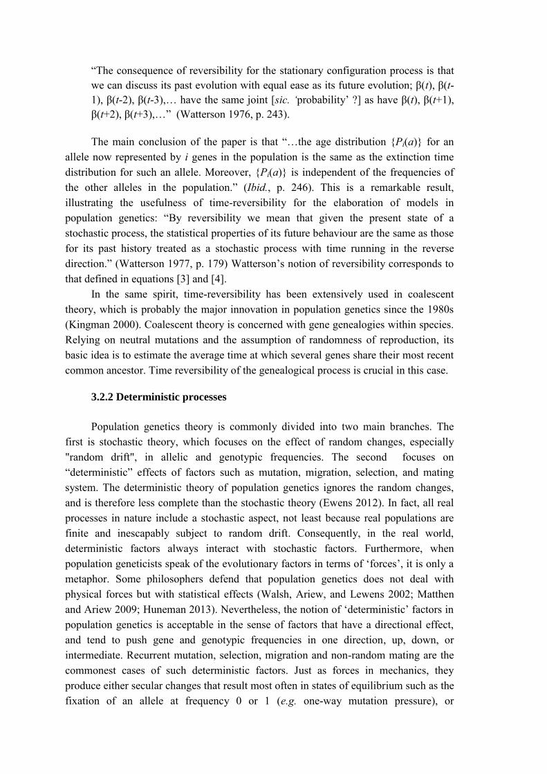
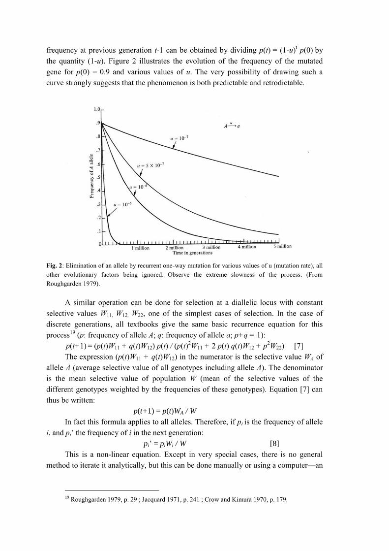
the quantity (1-u). Figure 2 illustrates the evolution of the frequency of the mutated

gene for p(0) = 0.9 and various values of u. The very possibility of drawing such a

curve strongly suggests that the phenomenon is both predictable and retrodictable.

Fig. 2: Elimination of an allele by recurrent one-way mutation for various values of u (mutation rate), all

other evolutionary factors being ignored. Observe the extreme slowness of the process. (From

Roughgarden 1979).

A similar operation can be done for selection at a diallelic locus with constant

selective values W11, W12, W22, one of the simplest cases of selection. In the case of

discrete generations, all textbooks give the same basic recurrence equation for this

process19

(p: frequency of allele A; q: frequency of allele a; p+q = 1):

p(t+1) = (p(t)W11 + q(t)W12) p(t) / (p(t)2W11 + 2 p(t) q(t)W12 + p

2W22) [7]

The expression (p(t)W11 + q(t)W12) in the numerator is the selective value WA of

allele A (average selective value of all genotypes including allele A). The denominator

is the mean selective value of population W (mean of the selective values of the

different genotypes weighted by the frequencies of these genotypes). Equation [7] can

thus be written:

p(t+1) = p(t)WA / W

In fact this formula applies to all alleles. Therefore, if pi is the frequency of allele

i, and pi‘ the frequency of i in the next generation:

pi’ = piWi / W [8]

This is a non-linear equation. Except in very special cases, there is no general

method to iterate it analytically, but this can be done manually or using a computer—an

19

Roughgarden 1979, p. 29 ; Jacquard 1971, p. 241 ; Crow and Kimura 1970, p. 179.

easy operation for anyone today with an application like Populus20

. Figure 6 (Appendix

3) gives the result of computer iterations from [7] for selection against a recessive allele

with strong selection. This is an illustration of a typically deterministic process.

Although analytical iteration is not accessible, it is possible to iterate backwards

generation-by-generation. Appendix 2.2 provides a demonstration of the possibility of

retrodiction in the case of a model of selection at a diallelic locus with

W11 > W12 > W22. This result could reasonably be extended to all possible fitness ratios,

because the backward equation is quadratic and its coefficients show that it has only

one positive solution (Anthony Edwards, personal communication). Therefore, at least

in this case, retrodiction is possible. Note that the backward equation is derived from

the forward equation. Appendix 2.2 also shows why reversibility is not satisfied for the

same model. This brings us to the issue of time-reversibility in population genetics.

3.2.2.2 Time-reversibility (mathematical sense)

The question of whether the deterministic models of population genetics are

reversible in the usual mathematical sense is the most delicate problem. If yes, the

‗laws‘ expressed by them should be unaffected by time reversal, that is substituting -t

for t in the equations (see section 3.1.2). Since the notion of ‗law‘ is important here, it

is worth recalling Elliott Sober‘s proposal. According to him, the traditional logical

empiricist concept of law requires that laws be statements that are both truly universal

(that is to say not referring to any place, time, or individual) and empirical. This

concept is inappropriate for various domains of science, especially evolution, where the

second condition (being an empirical statement) is questionable. For Sober (1997), the

process of evolution as studied in population genetics ―is governed by models that can

be known to be a priori true‖. These models are mathematical truths, which describe

how systems of specified type develop through time, whence Sober‘s expression

―process law‖. For instance, given Mendel‘s laws, and an operational definition of

notions such as recurrent mutation, selective value, etc., the process laws of population

genetics describe how these factors determine the trajectory of a population in the space

of gene frequencies. This viewpoint is endorsed here (Sober 1984, 1997; see also

Brandon 1997, and Gayon 2014).

The reason why the notion of law is important here is that time-reversibility is not

so much a property of a trajectory as a property of the law that governs the dynamics of

the system, and therefore underlies the trajectory. Strictly speaking, the property of

time-reversibility tells us nothing about the capacity of a given system to ‗return‘ to its

former state. This is not excluded, but will depend on the actual conditions imposed on

the system. Time-reversibility is a property of a law of transformation that applies to

20

Freely accessible on http://cbs.umn.edu/populus/download-populus. This application has been

developed by the College of Biological Sciences of the University of Minnesota for pedagogical

purposes. We thank Michel Veuille for giving us this information. For some (very) particular cases

where equation [7] is analytically tractable, see Hartl 1980, p. 209-210

transformations in both directions, whatever the actual fate of the system. For instance,

the reversibility of Newton‘s law (F = ma) does not mean that a given body submitted

to force F could effectively come back to a prior state, but that, if it did, the law would

still apply. Thus, mathematical reversibility evokes counter-factual prediction, not the

capacity of a given system to spontaneously return to a prior state (thermodynamic

reversibility, see below). Of course, the two notions are often closely related in actual

scientific practice, just as retrodictability and mathematical time-reversibility are often

connected. However, the concepts are distinct.

Returning now to the examples of recurrent mutation and selection, using exactly

the same models as in the previous paragraphs leads to the question ―Are the ‗laws‘

expressed in the recurrence equations time-reversible?‖

Case 1: Recurrent mutation

The position defended here is that the recurrence equation describing this process

is not time reversible. This thesis goes against a common intuition. Since it is one of the

simplest dynamic models in population genetics, it will be treated in detail21

.

To begin with, let us formally define the concept of time reversibility in a dynamic

system, the evolution of which can be described by a recurrence equation. We assume

that the state of a system x(t) at time t is a function of the p previous states:

x(t) = f (x(t-1), x(t-2),…, x(t-p)) [9]

Given that [9] is time-reversible for any sequence (x(0), x(1),…, x(T)) solution of

[9], so the reverse sequence (x(T), x(T-1),…, x(0)) is also a solution of [9].

Before applying this definition to the one-way recurrent mutation model, an example of

a recurrence equation that satisfies our definition of time-reversibility will first be

given.

Consider the following recurrence equation:

x(t+2) = 2 x(t+1) – x(t) + 1 [10]

It can easily be checked that the sequence (0, 1, 3, 6, 10, 15) is a solution of [10].

x(0) = 0 (initial condition)

x(1) = 1 (initial condition)

x(2) = (2 x 1) – 0 + 1 = 3

x(3) = (2 x 3) – 1 + 1 = 6

x(4) = (2 x 6) – 3 + 1 = 10

x(5) = (2 x 10) – 6 + 1 = 15

Surprisingly, the reverse sequence (15, 10, 6, 3, 1, 0) is also a solution of [10]:

x(0) = 15 (initial condition)

x(1) = 10 (initial condition)

x(2) = (2 x 10) – 15 + 1 = 6

21

The reasoning that follows should be credited to Jean-Philippe Gayon, who is warmly thanked

for his help.

x(3) = (2 x 6) – 10 + 1 = 3

x(4) = (2 x 3) – 6 + 1 = 1

x(5) = (2 x 1) – 3 + 1 = 0

More generally, for any sequence (x(0), x(1),…, x(T)) solution of [10], it is possible

to prove that the reverse sequence (x(T), x(T-1),…, x(0)) is also a solution of [10].

Therefore [10] is time-reversible.

Consider now the recurrence equation describing the evolution of the frequency p

of an allele A subject to recurrent mutation. As seen above [5], this equation is:

p(t+1) = (1–u) p(t)

The sequence (1, (1-u), (1-u) 2) is solution of [5] :

p(0) = 1 (initial condition)

p(1) = (1-u) x 1 = (1-u)

p(2) = (1-u) x (1-u) = (1-u)2

On the other hand, the reverse sequence ((1-u)2, (1-u), 1) is obviously not a

solution of [5] when u ≠ 0. If the initial condition is (1-u)2, then the sequence obtained

by applying [5] is

p(0) = (1-u)2 (initial condition)

p(1) = (1-u) x (1-u)2

= (1-u)3

p(2) = (1-u) x (1-u)3 = (1-u)

4

We conclude that equation [5] describing the evolution of a population under

recurrent mutation pressure is not time-reversible when u≠0 (in the case u=0, the

population never changes which is time reversible).

More generally, if any solution of [9] is strictly decreasing (respectively

increasing), then [9] is not time reversible.

However, we anticipate an objection. The practicing population geneticist might

say that reversing the direction of mutation (a→A instead of A→a) would amount to

‗reversing the process‘. To make things as symmetrical as possible, a rate of reverse

mutation equal to the rate of direct mutation could be taken, and begin with a frequency

of say 0.9 in both directions. A law of the same general form would describe the

‗reverse‘ dynamics and trajectory, with v (mutation rate for a→A) replacing u

(mutation rate for A→a). But this would be another process; because a crucial

parameter, with a different biological meaning (reverse mutation) has been introduced,

it is not the same law. Changing the direction of mutation does not amount to changing

the direction of time. ‗Reverse mutation‘ is a biological concept, which should not be

confused with the question of whether the process law describing the diffusion of a

‗recurrent‘ mutation is ‗reversible‘ or not.

Case 2: Basic models of selection

The basic equation to predict the evolution of gene frequencies for a diallelic

selection submitted to selection has been given in [7]. This recurrence equation is a

rather general one. It ignores the various possible relations between the selective

values, for instance: selection against a recessive gene (W22 < W12 =W11), selection

against the dominant allele (W11 < W22 = W12), incomplete dominance (W11 < W12 < W22

or W22 < W12 < W11), or advantage to the heterozygote (W12 superior to the two other

genotypic selective values). In all cases, selective values are assumed to be constant.

Now, given [8], Δpi can be calculated simply22

, giving:

Δ𝑝𝑖 =

(𝑊𝑖 −𝑊)

𝑊 [11]

with: pi: frequency of allele Ai; Wi : average selective value (or ―fitness‖) of the Ai

allele (= average selective value of all genotypes containing Ai ); W: average fitness of

the population (average fitness of all genes at this locus, or average fitness of all the

genotypes at the same locus in the population).

Equation [11] is of fundamental importance for the genetical theory of natural

selection. As underlined by Crow and Kimura (1990, p. 180), it shows that the rate of

change of gene frequency is proportional to: (1) the gene frequencies, pi (1-pi), which

means that a very rare or very common gene will change slowly, regardless of how

strongly it is selected; (2) the average excess in fitness of the Ai allele over the

population average (Wi – W), which can be either positive or negative. If Wi – W is

positive, the frequency of the allele will increase; if negative, it will decrease. Whether

Δpi always increases, or always decreases, or sometimes increases and sometimes

decreases will depend on the relations between the genotypic selective values W11, W12,

and W22.

Before commenting on reversibility, another crucial notion must be introduced. If the

selective values are kept constant, Δpi can be rewritten as:

𝛥𝑝𝑖 =

𝑝𝑖 1 − 𝑝𝑖

2𝑊

𝑑𝑊

𝑑𝑝𝑖 [12]

This famous equation is known as ―Wright‘s formula‖ (Wright 1937, 1940). It is

fundamental because it connects the change in gene frequency Δp, with the slope of the

function W (average fitness). It shows that if W is at a maximum with respect to p, then

Δp is zero, or in other words the population is at equilibrium. W is classically

interpreted as the ―fitness function‖ or the ―adaptive topography‖. Since W maximizes,

a population submitted to selection is seen as ―going uphill‖. Figures 3, 4, 5, 6, 7,

(Appendix 3) borrowed from Albert Jacquard (1971), give a clear graphic expression of

the connection between Δp and W in various cases; these are actually the most common

situations taught in an elementary course of population genetics. On these graphs, W11,

W12, W22 are the selective values (or ‗fitnesses‘). By convention, Jacquard has

systematically taken W11 ≤ W22, and p is the frequency of the unfavoured gene

(numbered ―1‖). This is why Δp is most often negative. (It would be equivalent to

observe the increase of the favoured gene; Δp would then be positive; but of course the

order of alleles on the graph should be inverted). The arrows in the figures show that W

22

See Crow and Kimura, 1970, p. 179-180.

is always ≥ 0 and is systematically maximized. Equilibrium is attained when W is

maximal; this maximal value of W corresponds to Δp = 0. In Figures 3, 4, 5, the

equilibrium is realized when p = 0 (the unfavoured gene disappears, the other gets

fixed). In Figure 6 (heterozygote inferiority), there are two stable equilibriums, p = 0

and p = 1, the outcome depending on the initial conditions). In Figure 7 (heterozygote

superiority), the population stabilizes for an intermediate value of p: selection maintains

variation. Figures 8 and 9 are examples of the trajectories of populations submitted to

two kinds of selective pressure abundantly realized in nature: selection against a

recessive allele (Figure 8), and selection with heterozygote superiority (Figure 9). In

each case, several curves are given, corresponding to selective pressures of varying

intensity. The trajectory given in Figure 8 corresponds to the dynamics represented in

Figure 5 (selection against a recessive). The trajectory given in Figure 9 corresponds to

the dynamics represented in Figure 7 (heterozygote superiority). The trajectories

represented in Figures 8 and 9 are the result of computer iterations from the basic

recurrence equation. As observed by Roughgarden (1979), it is remarkable that

equation [12] despite its important restrictive condition (constancy of selective values),

can generate so many different trajectories.

Are these models time-reversible? Formally, it would be useful here to provide a

detailed proof that the basic recurrence equation [7], or its special applications

(sometimes with simplifying assumption) to particular cases (e.g. Crow and Kimura

1970, equations 5.2.2, and 5.2.14 to 5.2.17), or the treatment of the same problems with

continuous time (e.g. Crow and Kimura 1970, eq. 5.2.8 to 5.2.11) are not time-

reversible. This will be treated in a future publication. For the time being, Appendix 2.2

provides a proof in the special case of a diallelic model with W11 > W12 > W22. It shows

that the dynamics of this system are retrodictable but not reversible. In fact the situation

is identical to that of recurrent mutation. In both cases, it is possible to derive a rule for

retrodiction, but this rule is obviously incompatible with the idea that the dynamic

equation is reversible.

Furthermore, it should be observed that all standard models of selection with

constant selective values describe dynamics that are driven by a maximizing function

(maximization W of the average selective value of the population). Therefore it seems

hard to imagine that such models could be used to describe a reverse transformation

obeying exactly the same law: what would it mean for a population to accomplish the

reverse trajectory with W minimized throughout? This would contradict the models. To

sum up, all elementary models of selection evoked in the present chapter are

deterministic and retrodictable, but they do not seem to describe a time-reversible

process.

One final observation on this subject. We mentioned earlier that in selective

models with constant genotypic selective values, the average selective value always

increases from generation to generation, until it becomes equal to zero when

equilibrium is attained, therefore ΔW ≥ 0. However, should this be understood strictly

or approximately? Is there room for oscillation, as was often suggested in elementary

courses of population genetics some decades ago, especially in the case of heterozygote

superiority (see Figure 7)? The idea was that the population rises through the adaptive

topography a little like a ball which runs down a bowl, goes up the other side of the

bowl, comes back, runs up again, etc. However, it has been demonstrated that there is

no room for oscillation (Roughgarden 1979). This comes as no surprise if selection

takes a population close to the fixation of one of the alleles: once the gene is fixed, no

variation is left, and therefore there is no room for further selection. But in the case of

heterozygote advantage, this is somewhat more surprising. Roughgarden (1979, p. 51-

53) notes that there is no possibility of ―overshoots that are so large as to prevent the

convergence to 𝑝 ‖. Therefore W is ≥ 0. No oscillation, no bounce. Although this is only

an intuitive comparison, this behaviour can be contrasted with the situation in classical

mechanics. If a moving body finds an obstacle on its way, one expects that it will

communicate a fraction of its movement to another body, and bounce. Nothing like this

is observed in standard models of selection: when the equilibrium point is reached, the

movement just stops. This is typical of highly directional and maximizing dynamics,

where reversion is hardly conceivable as long as the conditions remain the same.

3.2.2.3 ‘Physical’ or ‘thermodynamic’ reversibility

Physical reversibility is the possibility for a system to return spontaneously to a

previous state. Does this apply to population genetics? This subject will not be treated

here in detail. A few glimpses will suffice. Since Ronald Fisher, the directionality of

evolution under natural selection has been regularly compared with the directionality

implied by the Second Law of Thermodynamics. The Second Law asserts that

irreversible physical processes imply a unidirectional increase of entropy. In his

Genetical Theory of Natural Selection (1930), Fisher ‗immediately recognized certain

formal analogies between the mechanistic models introduced by Boltzmann (1896) to

analyse physical systems, and the selection models proposed by Darwin (1859) to

explain adaptation in biological systems‘ (Demetrius 2000). According to Demetrius,

Fisher‘s fundamental theorem of natural selection is indeed a directionality theorem.

This theorem states that ‗The rate of increase of fitness of any species is equal to the

genetic variance in fitness‘ (Fisher 1930, p. 50). By this formula, Fisher meant that the

speed of action of selection is a function of the additive genetic variance23

.

It is worth quoting Fisher here who compares his fundamental theorem with the Second

Law of Thermodynamics:

―Both are properties of populations, or aggregates, true irrespective of the nature

of the units which compose them; both are statistical laws ; each requires the

constant increase of a measurable quantity, in the one case the entropy of a

23

The additive genetic variance is the fraction of genetic variance attributable to the additive

effects of genes, ignoring the inter-allelic and inter-genotypic interactions (For detailed comments on

Fisher‘s fundamental theorem, see Price 1972; from a historical point of view, see Gayon 1998, Chap. 9).

physical system and in the other the fitness, measured by m, of a biological

population. As in the physical world we can conceive of theoretical systems in

which dissipative forces are wholly absent, and in which the entropy

consequently remains constant, so we can conceive, though we need not expect to

find, biological populations in which the genetic variance is absolutely zero, and

in which fitness does not increase.‖ (Fisher [1930] 1958, p. 39)

In spite of these resemblances24

, Fisher‘s objective was in fact to emphasize the

differences between the Second Law of Thermodynamics and his theorem. Among the

five differences that he mentions, one is of special interest for our subject: ―Entropy

changes are exceptional in the physical word in being irreversible, while irreversible

evolutionary changes form no exception among biological phenomena‖ (Fisher, ibid.,

p. 40).

In fact, modern population biologists, or at least some of them, compare entropy

and fitness more literally than Fisher used to. A stimulating example is Lloyd

Demetrius, who proposes an adaptation of the concept of entropy to evolutionary

genetics and ecology, and puts forward the concept of ―evolutionary entropy‖: a

measure of the dispersion of the age of the ancestors of a randomly chosen newborn.

Demetrius‘ concept of evolutionary entropy is an explicit attempt to overcome the

obvious difference between statistical thermodynamics and population biology;

thermodynamics deals with the properties of populations of inert particles, whereas

population biology treats the properties of populations of living objects which

reproduce, and therefore grow. To overcome this difficulty, Demetrius points to a

―formal correspondence‖ between the thermodynamic variables and the population

parameters intervening in population biology: ―growth rate‖ corresponds to free energy;

24

It is worth adding that in 1941, Fisher had a controversy with Wright about the meaning of his

‗fitness function‘ or ‗adaptive topography‘. Commenting on this equation, Fisher wrote: ‗Wright‘s

conception embodied in equation (6) (eq. [12] in the present paper]) that selective intensities are

derivable, like forces in a conservative system, from a simple potential function dependent on the gene

ratios of the species as a whole, has led him to extensive but untenable speculations.‘ (Fisher 1941). Thus

Fisher denies that [12] is a potential function describing a conservative system—a position also assumed

by Crow and Kimura in their 1970 textbook. However Fisher‘s objection is formulated in a context

where the adaptive topography is supposed to describe the behaviour of the species for all gene ratios. In

reality, Wright‘s equation is valid only for a diallelic locus with constant selective values (Edwards

2000). Wright acknowledged this when he gave the equation for the first time in 1937, but he eventually

extended it to multi-allelic loci without providing proof. He also suggested that this equation could be

related to his notion of ‗adaptive landscape‘, a notion that takes into account the entire genome.

Populations are then seen as pushed towards a ‗peak‘ by W, the average selective value, an ever-

increasing quantity (For more on this controversy, see Gayon 1998, Chap. 9). However, as noted by

Edwards (2000), it is not clear at all that, even in the simplest case of a diallelic locus, W is a potential

surface: ‗Wright‘s mistake, repeated by Crow and Kimura, was to interpret his non-standard partial

derivative 𝜕𝑤 𝜕 𝑞𝑖 as ―the slope of w in the direction where the relative frequencies of the other alleles

do not change‖ (Crow and Kimura, 1970), whereas in fact it is the rate of change of w in that direction,

but with respect to change in qi alone. This is not a gradient on the w-‗surface‘ at all, and the analogy of a

potential function, already tenuous because of the factor qi(1-qi), is thus in reality even more remote.‘

(Edwards 2000, p. 68-69).

―generation time‖ corresponds to inverse temperature; ―evolutionary entropy‖

corresponds to thermodynamic entropy. Then, both situations follow the same

equations with the appropriate variables (Demetrius 2000). Demetrius‘ basic intention

is to offer an alternative to Fisher‘s conception of directional change in mean fitness:

Fisher‘s fundamental theorem is based on the relative viability of individuals within the

population; Demetrius takes into account the absolute survival and reproduction of

populations. In Demetrius‘ terms, ―Darwinian fitness is completely described by

evolutionary entropy, a demographic variable which measures the heterogeneity in the

age of reproducing individuals in the population.‖ (Demetrius 2000, p. 2) Moreover,

―[evolutionary] entropy characterizes Darwinian fitness, the efficiency with which a

population acquires and converts resources into viable offspring. Accordingly, entropy

predicts the outcome of natural selection in populations subject to different classes of

ecological constraints.‖ (Demetrius, Legendre, and Harremoës 2009) We acknowledge

that we feel rather uncertain about the precise sense in which ―evolutionary entropy‖

and entropy in the ordinary physical sense are correlated. As Demetrius & al.

recognize, evolutionary entropy is ―analogue of the Gibbs–Boltzmann entropy in

statistical thermodynamics‖. This analogy is grounded both in a formal similarity of

equations, and in the distinction between a microscopic25

and a macroscopic

description26

. Suffice to say that Demetrius‘s stimulating proposal represents just one

way among others to bridge the gap between population genetics and population

ecology, with its emphasis on absolute fitness, population density, and bounded vs.

unbounded population growth27

.

Demetrius‘ proposal will not be analysed further here. What matters for the

present paper is a consequence of his approach to the question of whether the

evolutionary dynamics are reversible or not in a thermodynamic (or thermodynamic-

like) sense. Rather than emphasizing the kind of unlimited evolutionary irreversibility

that Fisher favoured, Demetrius offers a tool that leaves room for both evolutionary

irreversible processes (characterized by unidirectional increase of evolutionary

entropy), and evolutionary reversible (or virtually stationary) processes. In such a

theoretical framework, the reversible/non reversible distinction is not an all or nothing

alternative, but rather a tool for describing the dynamics of evolutionary change

(Demetrius 2000. For a comprehensive description of this field of research, see Weber,

Depew and Smith 1988).

25

The uncertainty in the age of the mother of a randomly chosen newborn. 26

Darwinian fitness, the efficiency with which a population acquires and converts resources into

viable offspring. 27

Just to give an example : ‗In populations subject to bounded growth constraints,

demographically stable states are described by the condition of maximal entropy; in populations with

unbounded growth, demographically stable states are described by the condition of minimal entropy.

Under bounded growth conditions, entropy increases; under unbounded growth conditions, large

population size, entropy decreases; under unbounded growth conditions, small population size, the

change in entropy is random and non-directional‘ (Demetrius 2000, p. 7 ; see also Demetrius 1992, with

its explicit title, ‗Growth rate, population entropy and evolutionary dynamics‘)

This area of research is fascinating and innovative, but remains quite speculative

today. Are there real analogies with friction and heat dissipation in the models of

population genetics and ecology, or are these comparisons no more than suggestive

metaphors or mathematical analogies? This question will be left open (For a survey of

this field of research, see Weber, Depew and Smith 1988).

3.2.2.4 Other senses of reversibility in population genetics

The intuitive notion of reversibility (see above, 2.1, introduction) sometimes

encountered among population geneticists will now be reconsidered. For a population

geneticist, who usually works at a small evolutionary temporal scale, it seems obvious

that most often a given population can return to a prior state. For instance, if a recurrent

mutation spreads on its own and is fixed, in principle a reverse recurrent mutation can

do the same. If natural selection causes the expansion of an allele in the population, it is

always possible that selective pressure in the other direction returns the population to

its initial state. If random drift leads to the fixation of a mutated allele, a reverse

mutation followed by drift or selection may cause ‗reverse‘ evolution. And so on.

There is no doubt about the plausibility and effectiveness of such processes. But

they mean something different from the various senses of reversibility analysed above.

Recurrent reverse mutation has been discussed, consider now the case of selection. In

the haploid case, how far would an inversion of the selection coefficient amount to a

‗reversible process‘ in a technical sense close to time-reversibility? Appendix 2.1

provides a formal treatment of this problem in the simple case of haploid populations.

The method consists in replacing the selective values Wi (haploid populations) with the

inverse quantities 1/Wi in the recurrence equation. This inversion preserves the relative

values of the Ws, but in reverse order. The question then, is whether the inversion of the

fitness values preserves the ‗law‘ expressed in the recurrence equation or not. The

calculation shows that the dynamics of the initial equation is preserved with the new

parameters 1/Wi. Therefore, the ‗law‘ is preserved by time reversal, except for the

constants. This is not ‗time-reversibility‘ in the strict sense, but could be named weaker

time reversibility (for a definition, see Appendix, 1., 1.2, and example in 2.1).

Incidentally, this demonstration applies to as many alleles and corresponding selective

values as required.

Would the same methodology produce a similar case in the case of selection on

sexually reproducing diploid population? Certainly not. Suppose for instance that the

heterozygote is advantaged, ie. W12 greater than both W11 and W22. The dynamics of

such selection is represented in Figure 7. If the values of the Wij were inverted, i.e. if

the Wij were replaced by expressions of the form 1/ Wij, then we would have W12 smaller

than both W11 and W22. This would correspond to the dynamics represented in Figure 6

(underdominance), with an unstable equilibrium, and two possible equilibria (p = 0 and

p = 1). This is indeed a totally different dynamics. The same could be said of other

possible ratios for the Ws, except when 𝑊12 = 𝑊22𝑊11 (see Appendix 2.3)28

. In this

case, the heterozyogote has an intermediate value, where the term ‗weak time

reversibility‘ could be used. In the general case, selection on a diallelic locus is not

reversible in any sense, although it is retrodictable (see demonstration for 𝑊11 >

𝑊12 > 𝑊22 in Appendix 2.2).

3.3 Conclusions on reversibility in theoretical population biology

Although the analysis above remains somewhat sketchy and incomplete, the

conclusions that it suggests are quite straightforward:

- Reversibility in the sense of retrodictability (in fact an improper use of the word)

seems obvious for deterministic models, with possible exceptions in discrete time. It

does not apply to stochastic models.

- Time-reversibility is clearly instantiated in some important stochastic models; it

seems inadequate for deterministic models. In one case (selection in a haploid

population), one comes close to time-reversibility since a weaker definition than the

usual one is met. However, this subject would require more extensive and detailed

examination.

- Thermodynamic reversibility, which is a fascinating subject, remains mainly a matter

of speculation.

- In classical models of selection, the average selective W can hardly be interpreted as a

potential function (see n. 11).

4. Conclusions

Two broad conclusions can be drawn. The first conclusion bears on lawfulness in

evolutionary biology. Laws do not need to be empirically true statements of unlimited

universal scope; they can also be ―models that can be known to be true a priori‖ (Sober

1997). Not all mathematical truths are laws, only those that elaborate on the basis of

some empirically plausible conditions. For instance, if Mendelian inheritance is

assumed, and if such factors as mutation, migration, mating system and selection are

plausible evolutionary factors, then it is possible to derive the typical behaviour of a

population under specified conditions. The abstract descriptions obtained are

idealizations, no more and no less than those developed by the physical sciences. The

question of whether they are useful to predict the actual behaviour of populations or not

is irrelevant to their nomological status. They just say that, if conditions C1, C2,…, Cn

are met, then a specific behaviour should be observed. The Hardy and Weinberg

equilibrium is a good example: provided that the six conditions stated in 2.2 are

28

Hartl (1980, Figure 25, p. 212) gives a nice graphical representation of this fact, although his

intention is not to comment on reversibility. The figure comprises two graphs showing the effect of

selection when allele A is favoured and when allele a is favoured. In both cases 𝑊12 = 𝑊22𝑊11 , and

several initial frequencies for A are considered. The trajectories are symmetrical.

satisfied, then the genetic structure of a population is constant over time. Of course no

biologist believes that actual populations are infinite, but the model opens the

possibility of making other models that will explain the deviations as a function of

population size. Therefore the problem is not whether the HW equilibrium is strictly

true from an empirical point of view, but how useful it is for explaining and predicting

the behaviour of real populations, in combination with other models that will take into

account the fact that this or that condition is not met, and to which degree it is not met.

Nevertheless, the HW law remains a mathematical truth if the standard conditions are

met. Some philosophers might argue here that it would be wiser to give up the term

‗law‘ and just speak of ‗models‘. This is maybe the case. In practice, population

geneticists use the terms ‗law‘ and ‗model‘ indifferently to qualify the HW equilibrium.

In other cases (e.g. treatment of the effects of mutation, selection or population size),

they tend to prefer ‗model‘. We do not think that this is a crucial issue. Whatever the

outcome of such a discussion, one important conclusion of this chapter is that an

impressive number of results of theoretical population genetics consist in equilibria,

which qualifies population genetics as a genuine science able to identify properties of

invariance through transformation. The discovery of such properties has been a

distinctive feature of modern science since its inception.

In population genetics, invariance to transformation is mainly defined with

reference to the genetic structure of a population. Under a number of conditions, this

structure may stabilize. One of the most characteristic features of population genetics as

a field of research is indeed the search for ―trends towards equilibria‖. When browsing

through text-books, it is amazing to observe in population genetics the definition of the

equilibrium, and the estimation of the time required to come close to it, is declared to

be more important than the precise description of the trajectory. This is what Haldane

meant when he stated that a good deal of evolutionary theory deals with the ‗statics‘

rather than the ‗dynamics‘ of evolution (Haldane 1954).

The second conclusion of this enquiry comes to temper the first one. Time-

reversibility has also been said to be a major characteristic of modern science, with

special reference to classical mechanics. In the theory of population genetics, time-

reversibility is obviously and abundantly present in the treatment of stochastic

evolutionary processes. But this is a rather particular sense of reversibility (symmetry

of probability distributions in both directions of time). As far as the authors have been

able to judge from this first exploratory enquiry, time-reversibility in its mathematical

sense does not seem to be a property of the models describing deterministic

phenomena. But this problem will have to be examined in a more systematic way.

Deterministic models in population genetics are highly retrodictable but this property is

not identical to time-reversibility.

Time reversibility is a very impressive property of the equations of classical

mechanics in the case of fundamental forces. In classical mechanics, objects follow the

principle of inertia so that a homogeneous rectilinear movement does not require an

external cause. The structure of selection models in population genetics is different.

The changes in a population are directly driven by differences in fitness. If these

differences cease to be, then the changes in the population stop immediately. In this

sense, selection in population genetics is closer to a mathematized Aristotelian

mechanics than to classical mechanics. In classical mechanics energy is conserved and

is transferred from potential energy to kinetic energy and vice versa, which ensures the

time reversibility of the dynamics. In population genetics, Wright‘s equation describes

a gradient ascent akin to classical potentials, but there is no equivalent to the kinetic

energy that would enable the system to descend the gradient, which would be required

for time reversibility.

To end up, the present publication is the first part of a broader enquiry on

repetition and reversibility in evolution, both at the theoretical and the experimental

level. A further paper will examine the rather different problems raised by the issues of

the repeatability of experiments in experimental population biology, and of the capacity

of populations or species to return to a prior evolutionary state.

Acknowledgements

Maël Montévil‘s work is supported by a grant from the labex ―Who am I?‖. This

paper has benefited from extensive discussion and collaboration with Jean-Philippe

Gayon, who has been enormously helpful in clarifying the notion of time reversibility

from a mathematical point of view. We also thank Anthony Edwards, Pierre-Henri

Gouyon, and Michel Veuille. Their great competence in population genetics has been

very fruitful to our understanding of the issue of reversibility in population genetics

models. We also thank Edwards and Veuille or their careful reading of the text. We

thank Elliott Sober for his careful reading of the paper and for his fruitful comments.

Véronique Charrière is warmly thanked for her careful linguistic corrections and

suggestions.

Appendices

Appendix 1 provides a formal definition of symmetry by time reversal and of

retrodictability. Appendix 2 applies these definitions to some population genetics

models. Appendix 3 contains the figures 3, 4, 5, 6 and 7.

1. Time reversibility

As discussed in the body of the text, time reversibility corresponds intuitively to a

situation where the dynamics follow the same law before and after time reversal. Only

deterministic dynamics are considered here.

1.1 Continuous time

In continuous time, a dynamic is typically defined by differential equations. A fairly

general definition of differential equations is admitted here:

0 = F α1,… ,x,dx ∕ dt, d2x ∕ dt2,… , dnx ∕ dtn (1)

where the 𝛼𝑖 are parameters.

Mathematical notion of time reversibility

Time reversal means substituting –t to t in an equation. Time reversibility describes

situations where the equation 𝐹 is still met after time reversal; that is to say:

0 = F α1,… ,x,−1 × dx ∕ dt, −1 2d2x ∕ dt2,… , −1 ndnx ∕ dtn (2)

Weaker time reversibility

We propose a weaker notion of time reversibility, where F is preserved even though the

parameters 𝛼𝑖 are modified through time reversal. Thus, the criterion becomes:

0 = F α1' ,… ,x,−1 × dx ∕ dt, −1 2d2x ∕ dt2,… , −1 ndnx ∕ dtn (3)

A supplementary condition is required for this notion to have a theoretical meaning.

The 𝛼𝑖′ have to be possible values for the 𝛼𝑖 . For example if 𝛼1 is a mass 𝛼1

′ has to be a

positive number, but it may be different from 𝛼1.

Retrodictability

The Cauchy-Lipschitz theorem also called Picard–Lindelöf theorem, states that

under very general hypotheses on the regularity of 𝐹, there is only one trajectory which

goes through one initial condition. This theorem is the basis of the ability of the

differential equation to define a deterministic process, but it also ensures that we can

retrodict the past. Increasing or decreasing the time parameter makes no difference in

this theorem. Note, however, that solutions to differential equations may be valid only

for a limited time interval, either because a variable becomes infinite or takes a value

that has no physical or biological meaning.

As mentioned in the main text, the issue of dynamics sensitive to initial

conditions, such as the three-body problem in mechanics have not been discussed here.

Let us just mention that in these cases, the impossibility of a perfect measurement of

the initial conditions prevents empirical long term predictions and retrodictions because

small differences have significant consequences.

1.2 Discrete time

Dynamics defined by recurrence will now be discussed: 𝑝 𝑡 + 1 = 𝑔 𝑝 𝑡 .

Mathematical notion of time reversibility

The transitions 𝑡 to 𝑡 + 1 and 𝑡 + 1 to 𝑡 follow the same law, that is:

𝑝 𝑡 + 1 = 𝑔 𝑝 𝑡 → 𝑝 𝑡 = 𝑔 𝑝 𝑡 + 1 .

Weak time reversibility

By analogy with the continuous case, changes in the values of the parameters of 𝑔 in

this weaker notion of time reversibility are allowed:

𝑝 𝑡 + 1 = 𝑔 𝑝 𝑡 ,𝛼𝑖 ,… → 𝑝 𝑡 = 𝑔 𝑝 𝑡 + 1 ,𝛼𝑖′ ,… .

Note also that the new parameters must have a physical or biological meaning.

Example: 𝑝 𝑡 + 1 = 𝑝 𝑡 ∕ 2 → 𝑝 𝑡 = 2𝑝 𝑡 + 1 . In this case 𝛼 = 1 ∕ 2 and 𝛼′ = 2.

See the next case for a dynamic that does not meet this criterion.

Retrodictability

Retrodictability corresponds to the fact that the reverse dynamic is deterministic. A

system is retrodictable when a function h exists that satisfies:

𝑝 𝑡 + 1 = 𝑔 𝑝 𝑡 ,𝛼,… → 𝑝 𝑡 = ℎ 𝑝 𝑡 + 1 ,𝛼′ ,…

Function ℎ may be completely different from 𝑔 (even though they are of course

related).

Example: 𝑝 𝑡 + 1 = 𝑝 𝑡 2 → 𝑝 𝑡 + 1 = 𝑝 𝑡 . This dynamic is retrodictable but

not reversible, even in the weak sense.

Counter example: 𝑝 𝑡 + 1 = 10𝑝 𝑡 − ⌊10𝑝 𝑡 ⌋, where ⌊𝑥⌋ is the integer part of 𝑥 (a

digit is lost at every step). For example 𝑃 0 = 0.97511..., 𝑃 1 = 0.7511.., 𝑃 2 =

0.511… But with 𝑃′ 0 = 0.87511..., we get 𝑃′ 1 = 0.7511…, which is identical to

P(1). This ambiguity prevents defining a deterministic reversed dynamic. This

deterministic dynamic does not enable retrodiction.

2. Application to models of population genetics

In this part, the reversibility of two classical models of selection in population

genetics are discussed. In one case (asexual haploid population), the dynamic is

reversible in the weak sense. In the second case (diploid, diallelic locus), the dynamic is

retrodictable but not reversible.

2.1 Asexual haploid population: a weakly reversible model

We start with a classical model of selection at a single locus in a haploid population. 𝑊𝑖

is the relative fitness of the allele 𝑖 and 𝑝𝑖 is the proportion of allele 𝑖 in the population.

W 𝑡 is the average fitness of the population at time 𝑡.

pi t + 1 = pi t

Wi

W t

(4)

To assess the properties of this dynamic with respect to time reversal, let us write 𝑝 𝑡

as a function of 𝑝 𝑡 + 1 , and let us compare the result with equation 4.

pi t = pi t + 1

W t

Wi

(5)

Equation (5) can also be written:

pi t = pi t + 1

1 ∕ Wi

1 ∕ W t

(6)

Here 1 ∕ 𝑊𝑖 seems to play the same role as 𝑊𝑖 in equation 4, therefore we can write

𝑊𝑖′ = 1 ∕ 𝑊𝑖 . However, we have to verify whether 1 ∕ W 𝑡 can be interpreted as the

mean fitness in the reversed dynamic W′ 𝑡 + 1 , where the new fitness coefficients are

the 𝑊𝑖′ .

By definition, we have :

1

W t =

N t

N t + 1 = W' t + 1

(7)

It is also possible to do this computation on the basis of the analytical expression of

𝑊 𝑡 which leads to the same result. Then we can conclude that:

pi t = pi t + 1

Wi'

W' t + 1

(8)

This equation has exactly the same form as equation (4). Therefore the dynamic is

weakly reversible.

2.2 Sexual diploid population: a retrodictable but irreversible model

A population with two alleles at a single locus is now considered. The relative fitnesses

are 𝑊11 ≠ 0 and 𝑊22 ≠ 0 for homozygotes and 𝑊12 for heterozygotes, and 𝑊11 >

𝑊12 > 𝑊22 . W 𝑡 is the average fitness of the population. 𝑝 and 𝑞 are the proportions

of the first and second allele in the population. A classical model for this situation is

then:

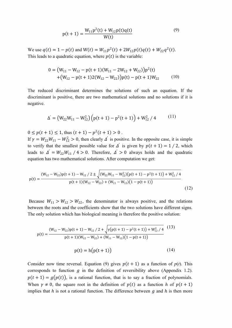
p t + 1 =

W11p2 t + W12p t q t

W t

(9)

We use 𝑞 𝑡 = 1 − 𝑝 𝑡 and W 𝑡 = 𝑊11𝑝2 𝑡 + 2𝑊12𝑝 𝑡 𝑞 𝑡 + 𝑊22𝑞

2 𝑡 .

This leads to a quadratic equation, where 𝑝 𝑡 is the variable:

0 = W11 − W12 − p t + 1 W11 − 2W12 + W22 p2 t

+ W12 − p t + 1 2 W12 − W22 p t − p t + 1 W22 (10)

The reduced discriminant determines the solutions of such an equation. If the

discriminant is positive, there are two mathematical solutions and no solutions if it is

negative.

Δ' = W22W11 − W122 p t + 1 − p2 t + 1 + W12

2 ∕ 4 (11)

0 ≤ 𝑝 𝑡 + 1 ≤ 1, thus 𝑡 + 1 − 𝑝2 𝑡 + 1 > 0 .

If 𝛾 = 𝑊22𝑊11 −𝑊122 > 0, then clearly 𝛥′ is positive. In the opposite case, it is simple

to verify that the smallest possible value for 𝛥′ is given by 𝑝 𝑡 + 1 = 1 ∕ 2, which

leads to 𝛥′ = 𝑊22𝑊11 ∕ 4 > 0. Therefore, 𝛥′ > 0 always holds and the quadratic

equation has two mathematical solutions. After computation we get:

p t =

W12 − W22 p t + 1 − W12 ∕ 2 ± W22W11 − W122 p t + 1 − p2 t + 1 + W12

2 ∕ 4

p t + 1 W12 − W22 + W11 − W12 1 − p t + 1

(12)

Because 𝑊11 > 𝑊12 > 𝑊22 , the denominator is always positive, and the relations

between the roots and the coefficients show that the two solutions have different signs.

The only solution which has biological meaning is therefore the positive solution:

p t =

W12 − W22 p t + 1 − W12 ∕ 2 + γ p t + 1 − p2 t + 1 + W122 ∕ 4

p t + 1 W12 − W22 + W11 − W12 1 − p t + 1

(13)

p t = h p t + 1

(14)

Consider now time reversal. Equation (9) gives 𝑝 𝑡 + 1 as a function of p(t). This

corresponds to function 𝑔 in the definition of reversibility above (Appendix 1.2).

𝑝 𝑡 + 1 = 𝑔 𝑝 𝑡 , is a rational function, that is to say a fraction of polynomials.

When 𝛾 ≠ 0, the square root in the definition of 𝑝 𝑡 as a function ℎ of 𝑝 𝑡 + 1

implies that ℎ is not a rational function. The difference between 𝑔 and ℎ is then more

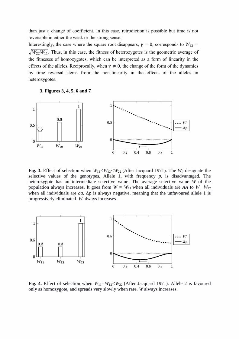
than just a change of coefficient. In this case, retrodiction is possible but time is not

reversible in either the weak or the strong sense.

Interestingly, the case where the square root disappears, 𝛾 = 0, corresponds to 𝑊12 =

𝑊22𝑊11 . Thus, in this case, the fitness of heterozygotes is the geometric average of

the fitnesses of homozygotes, which can be interpreted as a form of linearity in the

effects of the alleles. Reciprocally, when 𝛾 ≠ 0, the change of the form of the dynamics

by time reversal stems from the non-linearity in the effects of the alleles in

heterozygotes.

3. Figures 3, 4, 5, 6 and 7

Fig. 3. Effect of selection when W11<W12<W22 (After Jacquard 1971). The Wij designate the

selective values of the genotypes. Allele 1, with frequency p, is disadvantaged. The

heterozygote has an intermediate selective value. The average selective value W of the

population always increases. It goes from W = W11 when all individuals are AA to W W22

when all individuals are aa. p is always negative, meaning that the unfavoured allele 1 is

progressively eliminated. W always increases.

Fig. 4. Effect of selection when W11=W12<W22 (After Jacquard 1971). Allele 2 is favoured

only as homozygote, and spreads very slowly when rare. W always increases.

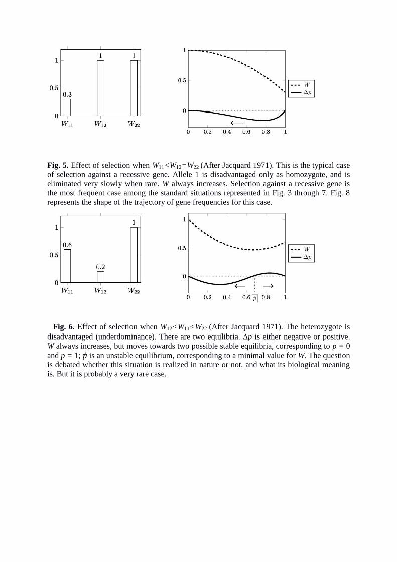
Fig. 5. Effect of selection when W11<W12=W22 (After Jacquard 1971). This is the typical case

of selection against a recessive gene. Allele 1 is disadvantaged only as homozygote, and is

eliminated very slowly when rare. W always increases. Selection against a recessive gene is

the most frequent case among the standard situations represented in Fig. 3 through 7. Fig. 8

represents the shape of the trajectory of gene frequencies for this case.

Fig. 6. Effect of selection when W12<W11<W22 (After Jacquard 1971). The heterozygote is

disadvantaged (underdominance). There are two equilibria. p is either negative or positive.

W always increases, but moves towards two possible stable equilibria, corresponding to p = 0

and p = 1; 𝑝 is an unstable equilibrium, corresponding to a minimal value for W. The question

is debated whether this situation is realized in nature or not, and what its biological meaning

is. But it is probably a very rare case.

Fig. 7. Effect of selection W11<W22<W12 (After Jacquard 1971). Known as overdominance or

‘advantage of the heterozygote’. There are two unstable equilibria, p = 0 and p = 1, and one

stable equilibrium, 𝑝 , corresponding to a maximal value for W, which always increases. p is

either negative or positive. This is the best-known polymorphic equilibrium, with ample proof

of its existence in nature.

Fig. 8. Selection against a recessive allele (from Roughgarden 1979). Compare with Fig. 4,

which gives the underlying dynamics. As almost all trajectories in models of selection with

discrete generations, this trajectory is obtained by computer iteration. s is the ‗selection

coefficient‘. The greater s is, the stronger the selection against the genotype. This is a

convenient way of treating the relative selective values. If the selective value of the favoured

genotype(s) is 1, the selective value of the unfavoured genotype (here the recessive

homozygote) is 1 – s.

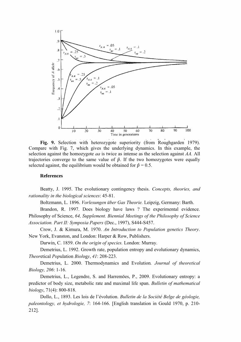
Fig. 9. Selection with heterozygote superiority (from Roughgarden 1979).

Compare with Fig. 7, which gives the underlying dynamics. In this example, the

selection against the homozygote aa is twice as intense as the selection against AA. All

trajectories converge to the same value of 𝑝 . If the two homozygotes were equally

selected against, the equilibrium would be obtained for 𝑝 = 0.5.

References

Beatty, J. 1995. The evolutionary contingency thesis. Concepts, theories, and

rationality in the biological sciences: 45-81.

Boltzmann, L. 1896. Vorlesungen über Gas Theorie. Leipzig, Germany: Barth.

Brandon, R. 1997. Does biology have laws ? The experimental evidence.

Philosophy of Science, 64, Supplement. Biennial Meetings of the Philosophy of Science

Association. Part II: Symposia Papers (Dec., 1997), S444-S457.

Crow, J. & Kimura, M. 1970. An Introduction to Population genetics Theory.

New York, Evanston, and London: Harper & Row, Publishers.

Darwin, C. 1859. On the origin of species. London: Murray.

Demetrius, L. 1992. Growth rate, population entropy and evolutionary dynamics,

Theoretical Population Biology, 41: 208-223.

Demetrius, L. 2000. Thermodynamics and Evolution. Journal of theoretical

Biology, 206: 1-16.

Demetrius, L., Legendre, S. and Harremöes, P., 2009. Evolutionary entropy: a

predictor of body size, metabolic rate and maximal life span. Bulletin of mathematical

biology, 71(4): 800-818.

Dollo, L., 1893. Les lois de l‘évolution. Bulletin de la Société Belge de géologie,

paleontology, et hydrologie, 7: 164-166. [English translation in Gould 1970, p. 210-

212].

Edwards, A. W. F. 1977. Foundationsof Mathematical Genetics. Cambridge

(UK): Cambridge University Press.

Edwards, A. W. F. 2000. Sewall Wright‘s equation 𝛥𝑞 = 𝑞 1 − 𝑞 𝜕𝑤 𝜕𝑞 2𝑤.

Theoretical Population Biology, 57: 67-70.

Ewens, W. 2012. James F. Crow and the Stochastic Theory of Population

Genetics. Genetics, 190, 2: 287-290.

Fisher, R. A. 1918. The correlation between relatives on the supposition of

Mendelian inheritance. Transactions of the Royal Society of Edinburgh, 52: 399-433.

Fisher, R. [1930] 1958. The Genetical Theory of Natural Selection. Oxford:

Clarendon, 2nd

edn 1958. New York: Dover.

Fisher, R. A. 1941. Average excess and average effect of a gene substitution.

Annals of Eugenics, 11: 53-63.

Gayon, J. 1998. Darwinism's Struggle for Survival : Heredity and the Hypothesis

of Natural Selection, Cambridge University Press, 1998.

Gayon, J. 2014. De la portée des théories biologiques. In: T. Martin, ed.,

Problèmes théoriques et pratiques en biologie évolutionnaire, Besançon, Presses

Universitaires de Franche Comté, p. 13-52

Gould, S. J. 1970. Dollo on Dollo‘s Law: Irreversibility and the Status of

Evolutionary Laws. Journal of the history of biology, 3, 2: 189-212.

Goux, J. M. 1979. Les modèles en génétique des populations. In: P. Delattre &

M. Thellier, eds., Élaboration et justification des modèles: applications en biologie,

Vol. II. Paris: Maloine, pp. 565-571.

Griffiths, Paul E. 1996. The Historical Turn in the Study of Adaptation. The

British Journal for the Philosophy of Science, 47, 4: 511-532.

Haldane, J . B. S. 1954. The Statics of Evolution. In: J. S. Huxley, A. C. Hardy,

and E. B. Ford (eds.). Evolution as a Process. London: Allen and Unwin, p. 109-121.

Hardy, G. H. 1908. Mendelian proportions in a mixed population. Science, 28:

49-50.

Hartl D. L. 1980 Principles of Population Genetics. Sunderland (MA, Sinauer

Associates.

Huneman, P. 2013. Assessing Statistical Views of Natural Selection: Is There a

Room for Non Local Causation?‖ Studies in History and Philosophy of Biological and

Biomedical Sciences 44: 604–612

Jacquard, A. 1971. Structures génétiques des populations. Paris, Masson. Engl.

Trans: The Genetic Structure of Populations, Springer-Verlag, 1974.

Kingman, J. F. C. 2000. Origins of the Coalescent: 1974-1982. Genetics, 56:

1461-1463.

Kelly, F. P. 2011. Reversibility and Stochastic Networks. Cambridge, Cambridge

University Press.

Lewontin, R. C. 1967. The Principle of Historicity in Evolution. In: Paul S.

Moorehead and Martin Kaplan, eds., Mathematical Challenges to the Neo-Darwinian

Interpretation of Evolution. Philadelphia: Wistar Institute Press, pp. 81-94.

Li, C. C. 1955. Population Genetics. Chicago: University of Chicago Press.

Longo, G. and Montévil, M. 2014. Perspectives on Organisms: Biological time,

symmetries and singularities. Coll. ‗Lecture notes in morphogenesis‘. Springer

Malécot, G. 1948. Les mathématiques de l’hérédité. Paris, Masson.

Matthen, M. and Ariew, A. 2009. Selection and Causation. Philosophy of

Science, 76: 201-224.

Montévil, M. and Mossio, M. 2015. Biological organisation as closure of

constraints. Journal of Theoretical Biology, 372: 179-191.

Price, G. R. 1972. Fisher‘s ‘fundamental theorem‘ made clear. Annals of Human

Genetics, 36, 129-140.

Roughgarden, J. 1979. Theory of Population Genetics and Evolutionary Ecology:

An Introduction. New York: MacMillan Publishing Co.

Simon H. 1977, Models of Discovery. Springer-Verlag.

Simpson, G. G., 1964. This View of Life. New York: Harcourt, Brace and World.

Sober, E. 1984. The Nature of Selection. Cambridge (MA): MIT Press.

Sober, E. 1997. Two Outbreaks of Lawlessness in Recent Philosophy of Biology.

Philosophy of Science, 64, Supplement. Biennial Meetings of the Philosophy of Science

Association. Part II: Symposia Papers (Dec., 1997), S458-467.

Walsh, D., Ariew, A. & Lewens, T, 2002. The Trials of Life: Natural Selection

and Random Drift. Philosophy of Science, 69: 452-473.

Watterson, G. A. 1976. Reversibility and the Age of an Allele. I. Moran‘s

infinitely Many Neutral Alleles Model. Theoretical Population Biology, 10: 239-253.

Watterson, G; A. 1977. Reversibility and the Age of an Allele. II. Two-allele

Models, with Selection and Mutation. Theoretical Population Biology, 12: 179-196.

Weber, J.S., Depew, D. & Smith, J.D. eds., 1988. Entropy, Information and

Evolution. Cambridge (MA): The MIT Press.

Weinberg, N. 1908. Ueber den Nachweis der Vererbung beim Menschen.

Jahreshriften des Vereins für Vaterländische Naturkunde in Württemburg, 64: 368-382.

Translated in: Papers in Human Genetics, ed. S. H. Boyer (1963), p. 4-15, Englewood

Cliffs, NJ: Prentice-Hall.

Williams, G. C. 1992. Natural Selection: Domains, Levels and Challenge., New

York, Oxford University Press.

Wright, S. 1921. Sytems of mating. Genetics, 6: 111-178.

Wright, S. 1937. The distribution of gene frequencies in populations. Proceedings

of the Natinal Academy of Science, 23: 307-320.

Wright, S. 1940. The statistical consequences of Mendelian heredity. In The New

Systematics , ed. J. Huxley. Oxford: Clarendon, p. 161–183.