Repaso de Matlab

Prof. Mark GlauserCreated by: David Marr

Info General

Ventana deComandos

Espacio deTrabajo

Historial deComandos

•La Ventana de Comandos es donde ingresas tu código, y donde Matlab muestra soluciones (A menos que le indiques lo contrario).•El Historial de Comandos enlista todos los comandos que ingresaste en la Ventana de Comandos, en caso que quieras volcer a tener acceso a ellos. Nota: El código previo puede corresrse otra vez haciendo click en la flecha hacia arriba o doble clicken el código de la ventana de historial de comandos•El Espacio de Trabajo enlista todas las variables que has creado en Matlab, indicando también su tamaño, numero de bytes y tipo. Otra forma de ver las variables actualmente en uso es ingresar el comando “whos” en la ventana de comandos.

Ayuda adicional

Si necesitas más ayuda en Matlab, puedes hacer click siempre que necesites sobre el signo de interrogación ubicado en la parte superior del programa, o digitar>> help funciónDonde función puede ser cualquier función para la cual Matlab tiene un archivo de ayuda.Por ejemplo:

>> help plot

Da informacíón en como usar la función “plot” así como hacerla que aparezca como tú deseas.

Comandos BasicosPara asignar una literal a un número específico, usa un signo igual como>>A=5

Esto no solamente asignará A igual al número 5, sino también lo escribirá por tí.Si no te interesa ver el resultado de un comando, digita un punto y coma al final .

Limpiando el Espacio de Trabajo

La función>>clear;Limpia todos los elementos en el espacio de trabajo.

Esto es útil si deseas borrar variables o algún otro elemento, si solamente deseas borrar un elemento>>clear A;

Insertar comentariosEn ocaciones deseará insertar comentarios en su códigopara recordar o indicar a otrso lo que está tratando de hacer. Esto se logra con un %, enseguida del cual se ingresa el comentario.Por ejemplo:

Usando el operador dos puntosYou can create a single row (or for that matter a single column) using the colon

operator. This is very important and useful feature of Matlab as will be seen. Por ejemplo, si quisieras crear una matriz renglón de cinco números, podrías usar el

comando:>>1:5El cual daría la salida1 2 3 4 5Nota que automaticamente asume numeros enteros. Si se deseara ir de uno a cinco

en incrementos de 0.2, se podría usar el comando:>>1:0.2:5El cual mdaría la salida 1 1.2 1.4 1.6 1.8 2… así hasta llegar al 5.If you wanted to set this equal to a variable, such as A, you would then be able to

access any number of the sequence you wanted using the commands:>>A=1:0.2:5>>B=A(3)Which would set your new variable “B” to the third instance of the row vector A,

giving an output ofB=1.4

Creating a matrixThere are many ways to create a matrix. Here are some examples:1. To create a matrix of all zeros with 2 rows and four columns

>>zeros(2,4)2. To create a matrix where all values are one

>>ones(# of rows, # of columns)3. To create a matrix of random values

>>rand(# of rows, # of columns)4. To create a matrix of random values with integers

>>fix(10*rand(# of rows, # of columns))Where fix always rounds down. I had to multiply by 10 in this case or all of

my values would have been rounded to zero!

As before, we can access any item in the matrix we want using “subscripts”

Sum and TransposeCreating a random matrix as before, we might get:1 23 4If we set this equal to “A” when creating it, we could sum up the columns by>>sum(A)To getans = 4 6

To find the transpose of the matrix A, use A’ to get:>> A=[1 2 ;3 4]A = 1 2 3 4>> A'ans = 1 3 2 4

Loading filesThere are two main ways to load files into Matlab.1. Using the load command. For example:

>>load data.txtwill load a file labeled data.txt into the workspace. To use this method, the file must either be in the current directory listed at the top of the program, or you can add the path of the file so that Matlab knows where to look for it. This function is:>>Addpath('D:\');Using the location of your file in place of D:\.

2. Using the Import Wizard found under File-Import Data.This method allows you to see what it is you are importing.

The variable created in Matlab will be of the same size as the original text or dat file, so if you started with two columns in the text file, you would end up with a matrix of two columns in Matlab.

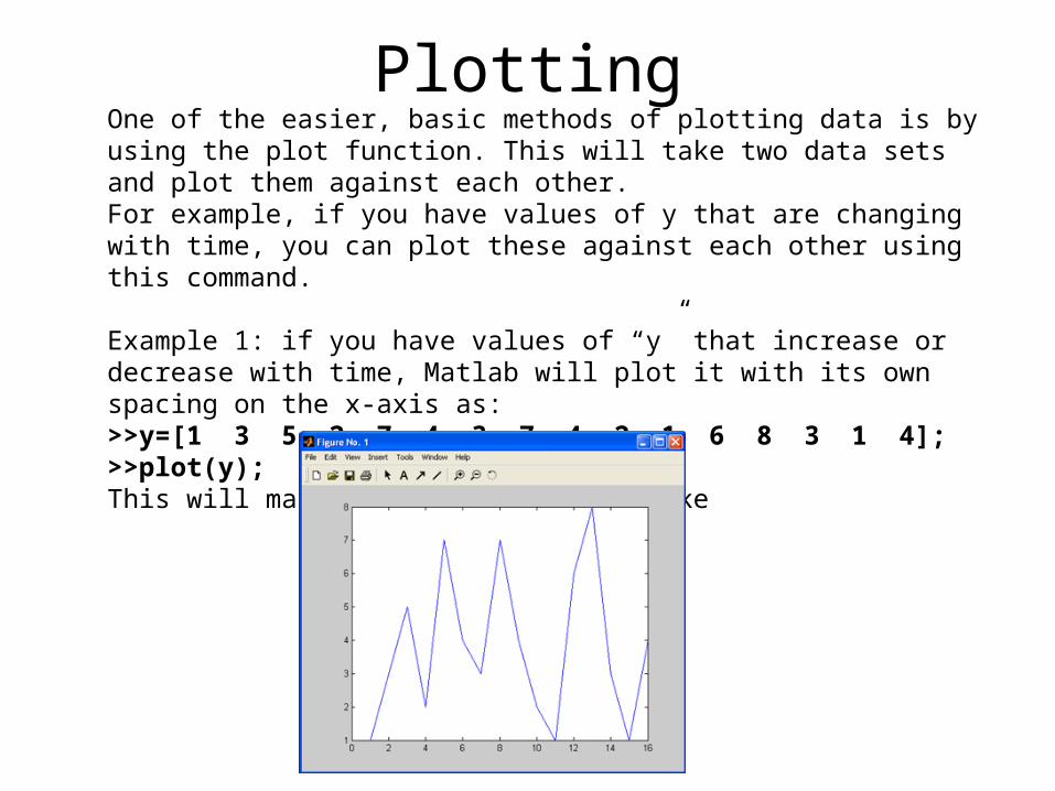
PlottingOne of the easier, basic methods of plotting data is by using the plot function. This will take two data sets and plot them against each other. For example, if you have values of y that are changing with time, you can plot these against each other using this command.

Example 1: if you have values of “y” that increase or decrease with time, Matlab will plot it with its own spacing on the x-axis as:>>y=[1 3 5 2 7 4 3 7 4 2 1 6 8 3 1 4];>>plot(y);This will make a graph that looks like

Plotting contd.If you want to plot values against other values on the x axis, you can tell Matlab what values to useExample:>>y=[1 3 5 2 7 4 3 7 4 2 1 6 8 3 1 4];>>x=[1 1.2 1.4 1.6 1.8 2.0 2.2 2.4 2.6 2.8 3 3.2 3.4 3.6 3.8 4];>>plot(x,y);Note: The x array could have bee created using the colon operator.This code will give you the result:

Plot FormatThere are a number of commands that control the plot format. In MATLAB help, look up commands “plot” and “axis.”

Plotting contd.

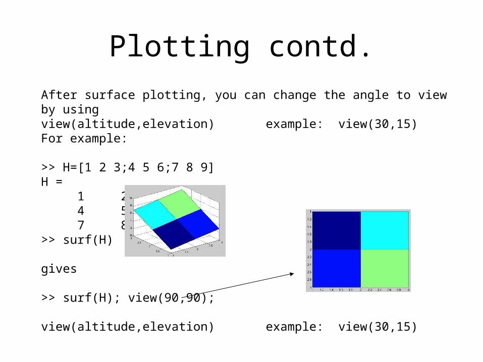
After surface plotting, you can change the angle to view by usingview(altitude,elevation) example: view(30,15) For example:

>> H=[1 2 3;4 5 6;7 8 9]H = 1 2 3 4 5 6 7 8 9>> surf(H)

gives

>> surf(H); view(90,90);

view(altitude,elevation) example: view(30,15)

Plotting contd.To get a feel for the values you just plotted, you can use the colormap command, so for the last example:

>> surf(H); view(90,90); colorbar;

To get

Example: Importing data and Plotting

Step 1: Either put the file you want to import into the current directory, or use the function “addpath” as shown earlier.

Step 2: If we assume the file is now in the current directory, we can bring it in by using >>load File1000.dat;Replacing File1000.dat with the name of your particular file. In my case, I have x values in the first column, y values in the second, u velocity in the third and v velocity in the fourth. I want to plot the first column on the x axis and the third column on the y axis. The name of the variable in this case is whatever the name of the file is. (Make sure the file type is correct. If this is a text file, you need to use “File1000.txt”)

Step 3: Use the plot command to choose what you want to plot>>plot(File1000(:,1), File1000(:,3))

Note: The : after File says to use the entire row while the 1 and 3 say to plot columns 1 and 3, so here I am plotting column 1 against column 3 as desired.

M-filesIt is often easier to create an external file with the code you want to run in it instead of typing it into the command window. If your code is long, or if you want to be able to edit it easily, you can create an “m” file (called this because files of this type have an m at the end- “MyCode.m”) that can be run in its entirety.

M-files contd.To create an m-file, use File - New - M-file which opens up another window. In this window you can insert your code, then save it to any location you want, although it is suggested to save it into your current directory. If saved in the current directory, you can run all code in the m file by typing the name in the command window- so if your file is called MyCode.m, you can run it using

>>MyCode

Another way to run your m-file is to use the “run” icon at the top of your m-file panel

•If you want to open an m-file in it’s own window, you can type

>>edit MyCode.m

•If you want to know what m-files can be opened (those in your current directory), click on “view” and click on the “Current Directory”.

•If you would wish to view the contents of an m file in the command window, you can use

>>type MyCode

Operators

< is less than<= is less than or equal to< is greater than>= is less than or equal to== is equal to~= is not equal to& is and| is or~ is not

Logical Arithmetic.’ Element by element transpose.^ Element by element exponentiation‘ Matrix transpose^ Matrix power+ Unary plus- Unary Minus.* Element by element multiplication./ Element by element right division.\ Element by element right division* Matrix multiplication/ Matrix right division\ Matrix left division

Random Tip

To move down a line without executing the line you just completed (In the command window), hold down shift while hitting the enter button.

If you want to reuse a previous typed command, use the “up” arrow key until the command you want comes up.

Defined variablesWhen you define a variable, such as when you type

>>x=2;

You can view this and all others by typing

>>whos

And a list of defined variables will be generated for you.

You can also see what variables have been created by looking in the “Workspace” assuming you have it open.

For loopsYou can create a loop in your program allowing you to run your code a specified number of times for a range of values using loops.For example, you can create an m-file with the code:

m=5n=7for i = 1:m

for j = 1:nH(i,j) = 1/(i+j);

endend

This code will create a 5 by 7 matrix H with values depending on the function 1/(i+j). Here I used two for loops together, although you can have as many or as few as you want.

Side note: you can plot a matrix such as this to see the values using the surf command as>>surf(H)

for pg149.m (Part 1)>>clearThe clear command resets the program before each run. For example, if you had previously set x=2 in a previous function, then it will remain defined as 2 until you use the clear command.>>figure (1); clfThe figure command opens(take a wild guess) a blank figure- in this case the first blank figure. The clf after the command clears the figure.>>figure (2); clfThis figure command opens a second blank figure.>>zeta=[0.05; 0.1; 0.15; 0.25; 0.5; 1.00; 1.25];This creates a seven dimensional vector named zeta. Think of zeta as a single column matrix with 7 rows.

for pg149.m (Part 2)>>r=[0: 0.01: 3]; ratio of the excitation frequency to the natural frequency of undamped oscillation. This creates a one-row matrix starting with zero, ending with 3 and including all numbers in between in sequences of 0.01>>for i=1:length(zeta),This begins a “for” statement that will run all statements between the “for” command and the “end” command on the given values of i, which in this case begins with one and continues until i reaches 7 (the length of the vector zeta)>>G=1./sqrt((1-r.^2).^2+(2*zeta(i)*r).^2); This defines the letter “G”, defined in chapter 3 as the magnitude of the frequency response, to its equation. Notice the period before the division and power- these are used in Matlab for element by element division and power. Looking closely, you notice no period before the “r”, which was defined earlier in the program as a matrix. Notice also that G will have different values for the various values of i.

for pg149.m (Part 3)

>>phi=atan2(2*zeta(i)*r,1-r.^2); %phase angle of the frequency response“atan(x)” is the arctangent of the elements of x. “atan2(x,y)” is the four quadrant arctangent of the real parts of the elements of x and y. The specifics of what atan2 2 does are unimportant, it should be viewed for now as simply the definition of another parameter that changes with the value of i.>>figure(1)This command brings forward the first figure and lets Matlab know that the following commands are referring to it.>>plot(r,G)This plots the current values of r and G on the figure

for pg149.m (Part 4)>>hold onHOLD ON holds the current plot and all axis properties so that subsequent graphing commands add to the existing graph. Using “hold off” would go back to the default way of overwriting the current figure.>>figure(2)This command brings forward the second figure and lets Matlab know that the following commands are referring to it.>>plot(r,phi)This plots the current values of r and phi on the figure>>hold onHOLD ON holds the current plot and all axis properties so that subsequent graphing commands add to the existing graph. Using “hold off” would go back to the default way of overwriting the current figure.>>end This function stops the for command once it has gone through all the the values of i.

for pg149.m (Part 5)>>figure(1)This command brings forward the first figure and lets Matlab know that the following commands are referring to it.>>title('Frequency Response Magnitude')This command gives the figure a title directly above the graph>>xlabel('\omega/\omega_n')This command labels the x axis. The \ before each “omega” lets Matlab know to use the symbol for omega instead of the word itself.>>ylabel('|G(i\omega)|')This command labels the y axis. The \ before each “omega” lets Matlab know to use the symbol for omega instead of the word itself.>>gridGRID, by itself, toggles the grid state of the current axes. To learn more about changing the grid, type “help grid” at the command line. In this case, it adds gridlines to our graph.

for pg149.m (Part 6)>>figure(2)This command brings forward the second figure and lets Matlab know that the following commands are referring to it.>>title('Frequency Response Phase Angle')This command gives the figure a title directly above the graph>>xlabel('\omega/\omega_n')This command labels the x axis. The \ before each “omega” lets Matlab know to use the symbol for omega instead of the word itself.>>ylabel('\phi(\omega)')This command labels the y axis. The \ before each “omega” lets Matlab know to use the symbol for omega instead of the word itself.

for pg149.m (Part 7)>>ha=gca;GCA means get handle to current axis. ha = gca returns the handle to the current axis in the current figure. The current axis is the axis that graphics commands like PLOT, TITLE, SURF, etc. draw to if issued.>>set(ha, 'ytick', [0: pi/2: pi])This sets the tick marks on the y axis from zero to pi in sections of pi/2.>>gridGRID, by itself, toggles the grid state of the current axes. To learn more about changing the grid, type “help grid” at the command line. In this case, it adds gridlines to our graph.>>set(ha, 'FontName','Symbol','ylim',[0 pi])This makes the labels print out the symbol pi and set the upper line at pi instead of showing graph above the upper line.>>set(ha, 'yticklabel',{'0';'p/2';'p'})This actually labels the y axis as 0, pi/2 and pi.

FFT- try on own if bored