Renewable Energy Cost of Generation Update INTERIM REPORT
272
Arnold Schwarzenegger Governor RENEWABLE ENERGY COST OF GENERATION UPDATE PIER INTERIM PROJECT REPORT Prepared For: California Energy Commission Public Interest Energy Research Program Prepared By: KEMA, Inc. August 2009 CEC-500-2009-084
Transcript of Renewable Energy Cost of Generation Update INTERIM REPORT

Arnold Schwarzenegger
Governor
RENEWABLE ENERGYCOST OF GENERATION UPDATE
PIER
INTE
RIM
PROJ
ECT R
EPOR
T
Prepared For: California Energy Commission Public Interest Energy Research Program
Prepared By: KEMA, Inc.
August 2009 CEC-500-2009-084


Prepared By: KEMA, Inc. Charles O’Donnell, Pete Baumstark, Valerie Nibler, Karin Corfee, and Kevin Sullivan Oakland, CA 94612 Commission Contract No. 500-06-014 Commission Work Authorization No: KEMA-06-020-P-R
Prepared For:Public Interest Energy Research (PIER) California Energy Commission
Cathy Turner Contract Manager
John Hingtgen, M.S. Project Manager Energy Generation Research Office Kenneth Koyama Office Manager Energy Generation Research Office
Thom Kelly Deputy Director ENERGY RESEARCH & DEVELOPMENT DIVISION Deputy Director Melissa Jones
Executive Director
DISCLAIMER
This report was prepared as the result of work sponsored by the California Energy Commission. It does not necessarily represent the views of the Energy Commission, its employees or the State of California. The Energy Commission, the State of California, its employees, contractors and subcontractors make no warrant, express or implied, and assume no legal liability for the information in this report; nor does any party represent that the uses of this information will not infringe upon privately owned rights. This report has not been approved or disapproved by the California Energy Commission nor has the California Energy Commission passed upon the accuracy or adequacy of the information in this report.


i
Preface
The California Energy Commission’s Public Interest Energy Research (PIER) Program supports public interest energy research and development that will help improve the quality of life in California by bringing environmentally safe, affordable, and reliable energy services and products to the marketplace.
The PIER Program conducts public interest research, development, and demonstration (RD&D) projects to benefit California.
The PIER Program strives to conduct the most promising public interest energy research by partnering with RD&D entities, including individuals, businesses, utilities, and public or private research institutions.
PIER funding efforts are focused on the following RD&D program areas:
• Buildings End‐Use Energy Efficiency
• Energy Innovations Small Grants
• Energy‐Related Environmental Research
• Energy Systems Integration
• Environmentally Preferred Advanced Generation
• Industrial/Agricultural/Water End‐Use Energy Efficiency
• Renewable Energy Technologies
• Transportation
Renewable Energy Cost of Generation Update is the interim report for the Renewable Energy Cost of Generation Update project (Contract Number 500‐06‐014, work authorization number KEMA‐06‐020‐P‐R) conducted by KEMA, Inc. The information from this project contributes to PIER’s Renewable Energy Technologies Program.
For more information about the PIER Program, please visit the Energy Commission’s website at www.energy.ca.gov/research/ or contact the Energy Commission at 916‐654‐4878.
Acknowledgement
Gerry Braun, PIER technical consultant, is acknowledged for his invaluable technical guidance and review of this project.
Please use the following citation for this report: O’Donnell, Charles, Pete Baumstark, Valerie Nibler, Karin Corfee, and Kevin Sullivan (KEMA). 2009. Renewable Energy Cost of Generation Update, PIER Interim Project Report. California Energy Commission. CEC‐500‐2009‐084.

ii

iii
Table of Contents
Executive Summary ........................................................................................................................... 1
1.0 Introduction .......................................................................................................................... 3
2.0 Project Approach ................................................................................................................. 5
2.1. Task 1: Technologies ..................................................................................................... 5
2.2. Task 2: Cost Drivers ...................................................................................................... 6
2.3. Task 3: Current Costs .................................................................................................... 6
2.4. Task 4: Expected Cost Trajectories .............................................................................. 7
2.4.1. Method ....................................................................................................................... 9
2.5. Task 5: Price/Cost Reconciliation ................................................................................. 10
2.6. Task 6: Community and Building Scale Renewable Energy Costs ........................ 11
3.0 Project Outcomes ................................................................................................................. 13
3.1. Technologies ................................................................................................................... 13
3.1.1. Technical and Analytical Critique of Reference Documents .............................. 13
3.1.2. Method for Selecting Technologies ........................................................................ 22
3.1.3. Utility‐Scale Technologies ....................................................................................... 23
3.1.4. Community‐Scale Technologies ............................................................................. 24
3.1.5. Building‐Scale Technologies .................................................................................... 24
3.2. Biomass ............................................................................................................................ 24
3.2.1. Technology Overview .............................................................................................. 24
3.2.2. Biomass Combustion – Fluidized Bed Boiler ........................................................ 27
3.2.3. Biomass Combustion – Stoker Boiler ..................................................................... 35
3.2.4. Biomass Cofiring ....................................................................................................... 42
3.2.5. Biomass Co‐Gasification IGCC ............................................................................... 47
3.3. Geothermal ...................................................................................................................... 52
3.3.1. Technology Overview .............................................................................................. 52
3.3.2. Geothermal – Binary ................................................................................................. 59
3.3.3. Geothermal – Flash ................................................................................................... 68
3.4. Hydropower.................................................................................................................... 72
3.4.1. Technology Overview .............................................................................................. 72
3.4.2. Hydro – Developed Sites Without Power ............................................................. 75
3.4.3. Hydro – Capacity Upgrade for Developed Sites With Power ............................ 80
3.5. Solar .................................................................................................................................. 84

iv
3.5.1. Technology Overview .............................................................................................. 84
3.5.2. Solar – Parabolic Trough .......................................................................................... 86
3.5.3. Solar – Photovoltaic (Single‐Axis) .......................................................................... 96
3.6. Wind ................................................................................................................................. 102
3.6.1. Technology Overview .............................................................................................. 102
3.6.2. Onshore Wind – Class 5 ........................................................................................... 106
3.6.3. Onshore Wind – Class 3/4 ........................................................................................ 117
3.6.4. Offshore Wind – Class 5 ........................................................................................... 117
3.7. Wave ................................................................................................................................ 123
3.7.1. Technology Overview .............................................................................................. 123
3.7.2. Ocean Wave ............................................................................................................... 125
3.8. Integrated Gasification Combined‐Cycle ................................................................... 127
3.8.1. Technology Overview .............................................................................................. 127
3.8.2. IGCC Without Carbon Capture (Single or Multiple 300 MW Trains) ............... 130
3.8.3. Carbon Capture and Sequestration ........................................................................ 136
3.9. Advanced Nuclear ......................................................................................................... 138
3.9.1. Technology Overview .............................................................................................. 138
3.9.2. WESTINGHOUSE – AP1000 ................................................................................... 143
4.0 Conclusions and Recommendations................................................................................. 157
5.0 References ............................................................................................................................. 159
6.0 Glossary ................................................................................................................................ 167
Appendix A Cost Data
Appendix B Responses to Workshop Comments
List of Figures
Figure 1. Utility‐scale fluidized bed gasifier ........................................................................................ 25
Figure 2. Biomass IGCC plant representation ...................................................................................... 26
Figure 3. Schematic diagram of biomass IGCC process ..................................................................... 26
Figure 4. Utility‐scale biomass fluidized bed gasifier ......................................................................... 27
Figure 5. Circulating fluidized bed schematic diagram ..................................................................... 28
Figure 6. Bubbling fluidized bed boiler ................................................................................................ 30

v
Figure 7. Stoker boiler schematic diagram ........................................................................................... 35
Figure 8. Flow schematic for a stoker boiler configuration ................................................................ 37
Figure 9. Biomass cofiring schematic for a pulverized coal boiler system ...................................... 42
Figure 10. Primary biomass cofiring locations ..................................................................................... 44
Figure 11. Process flow diagram for biomass gasification and conditioning for IGCC application ............................................................................................................................................................ 49
Figure 12. Binary power plant ................................................................................................................ 58
Figure 13. Flash power plant .................................................................................................................. 58
Figure 14. Financial impact of delay on exploration costs ................................................................. 62
Figure 15. Specific cost of power plant equipment vs. resource temperature ................................. 61
Figure 16. Economies of scale ................................................................................................................. 63
Figure 17. Impoundment hydropower ................................................................................................. 73
Figure 18. Diversion hydropower facility ............................................................................................ 74
Figure 19. Run‐of‐river hydropower facility ........................................................................................ 75
Figure 20. Hydropower costs for developed sites without power.................................................... 78
Figure 21. Hydropower costs for increasing capacity......................................................................... 82
Figure 22. Solar parabolic trough electric generating system ............................................................ 84
Figure 23. Simplified molten salt storage process diagram ............................................................... 85
Figure 24. Nellis Air Force Base PV installation .................................................................................. 86
Figure 25. Major cost categories for parabolic trough plant .............................................................. 91
Figure 26 Capital cost comparison ........................................................................................................ 94
Figure 27. Levelized O&M cost comparison ........................................................................................ 95
Figure 28. Solar module retail/price index, 125 watts and higher..................................................... 99
Figure 29. Solar power generation plant since 2006 over 20% cheaper .......................................... 100
Figure 30. Typical turnkey system price ............................................................................................. 101
Figure 31. A modern 1.5 MW wind turbine installed in a wind power plant ............................... 102
Figure 32. California wind resource map ........................................................................................... 103
Figure 33. Wind resource map of Northern California..................................................................... 104
Figure 34. Wind resource map of Southern California ..................................................................... 105

vi
Figure 35. Capacity factor trends of California utility wind sites ................................................... 106
Figure 36. Installed wind project costs over time .............................................................................. 109
Figure 37. Metal prices Jan. 2002 – Sept. 2007 (London Metal Exchange) ..................................... 111
Figure 38. U.S. dollar vs. euro, Jan. 1999 through April 2009 (European Central Bank) ............. 112
Figure 39. 2007 Project capacity factors by commercial operation date ......................................... 112
Figure 40. Onshore capacity factor by installed year and class ....................................................... 113
Figure 41. Annual and cumulative growth in U.S. wind power capacity ..................................... 114
Figure 42. Average cumulative wind and wholesale power prices over time .............................. 114
Figure 43. Installed wind project costs as a function of project size: 2006‐2007 projects ............. 115
Figure 44. European offshore wind installations ............................................................................... 118
Figure 45. European offshore wind growth and projections ........................................................... 120
Figure 46. Offshore capacity factor by installed year ........................................................................ 122
Figure 47. Point absorber ...................................................................................................................... 124
Figure 48. Oscillating water column ................................................................................................... 124
Figure 49. Overtopping ......................................................................................................................... 124
Figure 50. Attenuator ............................................................................................................................. 125
Figure 51. Typical oxygen‐blown IGCC process ............................................................................... 128
Figure 52. Actual installation (Buggenum, The Netherlands) with typical technological components indicated ................................................................................................................... 129
Figure 53. Bureau of Reclamation construction cost trends ............................................................. 134
Figure 54. Actual vs. Predicted Nuclear Reactor Capital Costs ...................................................... 139
Figure 55: Power Capital Cost Index – Nuclear and Non‐Nuclear Construction ......................... 141
Figure 56. Generations of nuclear energy ........................................................................................... 149
List of Tables
Table 1. Recent California legislation that may affect cost of generation .......................................... 1
Table 2. Cost driver analysis worksheet example ................................................................................. 9
Table 3. Comparison between 2009 KEMA analysis and 2007 IEPR ................................................ 16

vii
Table 4. Comparison of 2009 analysis with the CPUC GHG model data ........................................ 18
Table 5. Comparison between 2009 analysis with the RETI 1A Data ............................................... 20
Table 6. Central plant technology list for COG modeling project ..................................................... 23
Table 7. Installed CFB boiler capacity by country ............................................................................... 29
Table 8. Recent carbon steel pricing ...................................................................................................... 31
Table 9. Recent carbon steel pricing ...................................................................................................... 38
Table 10. Biomass stoker installed cost ranges – 2009 dollars per kW installed ............................. 41
Table 11. Coal‐fired generation plants with biomass cofiring ........................................................... 43
Table 12. Potential binary geothermal plant development in California (most likely sources) .... 64
Table 13. California and Nevada existing binary plants with capacity factor ................................ 65
Table 14. Fixed and variable O&M for binary geothermal power plants ........................................ 66
Table 15. Potential flash geothermal plant development in California (most likely sources)....... 69
Table 16. California and Nevada existing flash plants with capacity factor ................................... 70
Table 17. Fixed and variable O&M for flash geothermal power plants ........................................... 71
Table 18. Parabolic trough cost comparison ......................................................................................... 89
Table 19. Assessment of parabolic trough and power tower solar technology .............................. 91
Table 20. Comparison of total investment cost estimates ($/kWe): SunLab vs. S&L ..................... 94
Table 21. CSP plant capital cost breakdowns, 2005 ............................................................................. 95
Table 22. Annual CSP O&M cost breakdowns, 2005 .......................................................................... 96
Table 23. California utility wind plant installations since 2003 ....................................................... 108
Table 24. Size distribution and number of turbines over time ........................................................ 113
Table 25. Ocean wave energy cost data .............................................................................................. 127
Table 26. Gasification‐based power plant projects under consideration in the U.S. beyond 2010 .......................................................................................................................................................... 131
Table 27. Expected new nuclear power plant applications. ............................................................. 145
Table 28. Operators of U.S. reactors .................................................................................................... 147
Table 29. Nuclear decommissioning costs .......................................................................................... 154
Table 30. Nuclear plant construction spending profile (% of total instant cost per year) ........... 156

viii

ix
Abstract
This 2009 report updates the cost of generating electricity for technologies if built in California. California Energy Commission staff provides factors that affect costs, including cost assumptions, for 15 renewable technologies, coal‐integrated gasification, combined‐cycle, and nuclear power generation alternatives for utility‐scale generation technologies. These costs are useful in evaluating the financial feasibility of a generation technology and for comparing the costs of building and operating one particular energy technology with another. These estimates update the 2007 cost of generation, based on empirical data collected from operating facilities, research from primary sources, actual costs and surveys of expected costs from experts in the field, and reference documents. This report details a range of instant and installed costs with projected costs based on two years of significant growth in renewable technologies, changes in material costs, and inflation.
Keywords: Renewable energy, cost of generation, biomass, geothermal, hydropower, solar, parabolic trough, photovoltaic, PV, thermal solar, wind energy, ocean wave, integrated gasification combined‐cycle, IGCC, nuclear

x

1
Executive Summary This study examines the costs of renewable electricity generation in California to support the cost of generation modeling work of the Electricity Analysis Office. In addition to renewable electricity cost of generation assessment, nuclear and integrated gasification combined‐cycle generation are also examined. The California Energy Commission is tasked with developing robust cost of generation estimates, backed by solid research leveraging the full assessment of previous research on the cost of generation, cost drivers and trends, and expected cost trajectories for future costs. All of these data are then used by the Energy Commission to estimate the levelized cost of generation by technology.1
In the last several years, California has experienced tremendous activity in the renewable energy market, largely driven by several key pieces of legislation. The following table outlines some recent legislation that has been adopted that is likely to have a significant impact on the cost of generation for renewables as well as conventional generation.
Table 1. Recent California Legislation That May Affect Cost of Generation
Bill Author Year Passed
Summary
SB1 Murray (Chapter
132)
2006 SB 1 establishes in statute the California Solar Initiative with a goal of 3,000 megawatts of new solar produced electricity by the end of 2016. The California Solar Initiative Program has a $3.35 billion budget that will be administered by the California Public Utilities Commission, Energy Commission, and publicly owned utilities.
SB 107 Simitian (Chapter
464)
2006 SB 107 accelerates California’s Renewables Portfolio Standard targets by requiring California’s retail sellers of electricity to increase renewable energy purchases by at least 1 percent per year with a target of 20 percent renewable energy by 2010. It also requires the publicly owned utilities to file reports with the Energy Commission that outline their specific Renewables Portfolio Standard goals and progress towards the goals.
SB 1250
Perata (Chapter
512)
2006 SB 1250, combined with SB 107, continues the authorization of the Energy Commission’s ongoing use of public goods charge funds for the period of 2007-2012 for the continued operation of the Energy Commission’s Renewable Energy Program.
AB 2189
Blakeslee (Chapter
747)
2006 AB 2189 modifies the Renewables Portfolio Standard eligibility requirements for small hydroelectric generation facilities regarding efficiency improvements that result in increased capacity.
1 Levelized cost is the constant annual cost that is equivalent on a present‐value basis to the actual annual costs, which are themselves variable.

2
Bill Author Year Passed
Summary
AB 32 Núñez 2006 Global Warming Solutions Act – sets mandatory targets for greenhouse gas emission reductions. Commits to reducing greenhouse gas emissions to 2000 levels by 2010 (11 percent below business as usual), to 1990 levels by 2020 (25 percent below business as usual), and 80 percent below 1990 levels by 2050. Requires the California Air Resources Board and the Energy Commission to determine baselines and create systems to track greenhouse gas emissions.
Source: California Energy Commission
The ambitious goals – a Renewables Portfolio Standard of 20 percent by 2010 and 33 percent by 2020, 3,000 megawatts (MW) of photovoltaics installed within a decade, and an 11 percent reduction in greenhouse gas emissions by 2010 – are ambitious but achievable.
The Energy Commission’s work in the previous integrated energy policy reports confirm that the technical potential for renewables in California and the Western Electricity Coordinating Council region dwarfs these goals. In addition, developers of renewable energy power plants and the solar photovoltaic industry have responded to increased demand for renewable energy with enthusiasm. The Energy Commission intends to bridge the established policy backdrop and the surging renewable market to convert technical potential into reality.
KEMA, Inc. (KEMA) performed a detailed assessment of the generation technologies that might be available in the next 20 years. For each technology, KEMA assessed cost drivers and trends to develop input variables for the Energy Commission’s levelized cost model. To provide this information, researchers performed the following:
• Literature review and identification of renewable energy and two non‐renewable energy technologies likely to be deployed in California over the next 20 years, along with identification of the scale at which they are likely to be deployed.
• Cost drivers and trend analysis for each likely contributing technology and analysis of factors that determine the range (high, average, and low) of expected costs.
• Cost model input for utility‐scale technologies, including current nominal costs and plausible minimum and maximum costs for each utility‐scale technology, broken down into input variables that are used in the Energy Commission’s levelized cost analysis.
• Expected paths for future costs for utility‐scale generation technologies, plus a discussion of factors that determine these costs, as the basis for calculating levelized energy costs.
The four topics listed above are addressed for utility‐scale technologies in the interim project report. The final project report will also address community and building‐scale technologies as well as summarize key findings and recommendations.

3
1.0 Introduction
Renewable energy deployment in California is expected to accelerate in the near term in response to legislation identifying supply portfolio targets and climate mitigation targets. Related policy development must be based on the best possible economic information, especially the cost of bulk renewable energy electricity generation. In addition, two non‐renewable energy technologies are examined in support of the cost of generation modeling work of the Electricity Analysis Office and as comparisons to the renewable energy technologies. The two non‐renewable energy technologies included in this report are nuclear and integrated gasification combined‐cycle (IGCC). To provide this information, four fundamental topics were addressed:
• Literature review and identification of renewable energy and two non‐renewable energy technologies likely to be deployed in California over the next 20 years, along with identification of the infrastructure scales at which they are likely to be deployed.
• Cost drivers and trend analysis for each likely contributing technology and quantitative analysis of factors that determine the range of expected costs.
• Cost model input for utility‐scale technologies, including current nominal costs and plausible minimum and maximum costs for each utility‐scale technology, broken down into categories that are used in California Energy Commission (Energy Commission) levelized cost analysis.
• Expected paths for future costs for utility‐scale generation technologies, plus quantitative discussion of factors that determine these costs, as the basis for calculating levelized energy costs.
The four topics listed above are addressed for utility‐scale technologies in the interim project report. The final project report will also address community and building‐scale technologies and the following two topics:
• Reconciliation of currently quoted forward energy prices and currently estimated levelized costs, discussing the relative impact of various factors other than overnight construction cost that determine pricing. Reconciliation here refers to explaining the differences between prices and costs, identifying the factors that account for the differences, and providing estimates of the sizes of these factors.
• Costs and cost trajectories for community and building‐scale renewable energy technologies, along with minimum and maximum costs and trajectories for these scales.
The project was undertaken to achieve the following objectives:
• Critically review, adjust and augment the content of Appendix B of Energy Commission Report #CEC‐200‐2007‐011‐SF, December 2007 (Comparative Costs of California Central

4
Station Electricity Generation Technologies, Klein and Rednam) in order to create comparable information for the 2009 Integrated Energy Policy Report (IEPR).
• Update renewable energy and non‐renewable energy inputs for use in the Energy Commission’s Cost of Generation Model, used in preparing the 2009 IEPR.
• Reconcile price and cost information for representative utility‐scale power purchases.
• Estimate costs and trajectories for community and building‐scale technologies.
The following section describes the project approach followed by a section on project outcomes. The Project Outcomes section of the report includes an introduction to the technologies that were selected with the sections following organized by technology.

5
2.0 Project Approach
This section discusses the tasks the research team undertook and what the team did to accomplish the project objectives.
2.1. Task 1: Technologies The research team undertook the following activities:
• Conducted a technical and analytical critique of reference documents, including:
ο Comparative Costs of California Central Station Electricity Generation Technologies2 published by the California Energy Commission in December 2007.
ο Costs and supply curves generated in support of California Public Utilities Commission (CPUC) Greenhouse Gas (GHG) Modeling Project. Final results and GHG Calculator v2b from E3.3
ο Costs estimates found and used in the RETI Phase 1A and 1B reports by Black & Veatch in Renewable Energy Transmission Initiative Phase 1A.4
• Recommended utility‐scale RE technologies for cost analysis with technical and market justification. Utility‐scale RE technologies are generally defined as those over 20 MW.
• Identified the primary existing commercial embodiment of each utility‐scale technology in California. The term commercial embodiment is intended to describe the most prevalent commercially available application of a technology. As an example, in the case of solar thermal power, the primary existing application is concentrating parabolic trough collectors, augmented by natural gas‐fired boilers and supplying heat to steam Rankine power plants in the 50 MW to 80 MW size range.
• Identified the expected primary commercial embodiment in 2018.
The research team will revisit Task 1 for the community and building‐scale technologies in the second phase of the project and include findings in the final project report.
2 Klein, Joel and Anitha Rednam. Comparative Costs of California Central Station Electricity Generation Technologies. California Energy Commission, Electricity Supply Analysis Division, CEC‐200‐2007‐011, December 2007. http://www.energy.ca.gov/2007publications/CEC‐200‐2007‐011/CEC‐200‐2007‐011‐SF.PDF.
3 GHG Calculator v2b, updated on 5/13/08. http://www.ethree.com/CPUC_GHG_Model.html.
4 Black & Veatch. Renewable Energy Transmission Initiative Phase 1A (Draft Report). Black & Veatch, RETI Stakeholder Steering Committee, Project Number 149148.0010, March 2008. http://www.energy.ca.gov/2008publications/RETI‐1000‐2008‐001/RETI‐1000‐2008‐001‐D.PDF.

6
Please also note that this study provides estimates for cost of generation technologies but does not provide levelized life‐cycle cost estimates for the various energy technologies.5
2.2. Task 2: Cost Drivers For each of the utility‐scale technologies identified in Task 1, the research team identified:
• Market and industry changes since August 2007 that have materially affected costs.
• Current trends that will materially affect future costs.
• Primary general and California‐specific cost drivers (e.g., plant scale, global industry manufacturing scale, resource quality, plant location, capacity factor in case of storage coupled plants, overnight cost).
2.3. Task 3: Current Costs For each of the utility‐scale technologies identified in Task 1, the research team identified:
• Nominal 2009 costs in the format required for the Energy Commission’s levelized Cost of Generation model.
• Plausible minimum, average, and maximum costs with technical justification. To the extent possible, plausible maximum is defined as a cost more than one competitive player would be willing to pay, and plausible minimum is defined as is the least cost recorded absent hidden subsidies. In some cases, unique site characteristics were also considered.
The process for compiling data–of the plausible minimum, average, and maximum cost cases–was discussed between the research team and Energy Commission staff. Establishing ranges between minimum, average, and maximum costs circumscribes the range of market costs that would reasonably be encountered in the actual development, construction, and operation within each technology.
For each technology, size ranges were identified for total plant capacity to determine minimum, average, and maximum plant capacities in megawatts (MW). Plant capacity factors and forced outage rates were also defined using minimum, average, and maximum values, reflecting the ranges identified through researched values. North American Energy Reliability Corporation (NERC)/Generating Availability Data System (GADS) fleet reliability data were used for technologies where data was available, and in the case of wind, solar, and biomass technologies, other research sources were identified. Plant heat rates and fuel usage data were similarly modeled for low/average/high cases, based on actual operating plant characteristics; data was compiled for each fossil technology fuel usage reflecting in‐service values for generating plants.
5 Levelized life‐cycle cost estimates include the total cost of a project from construction to retirement and decommissioning. The research teamʹs cost estimates for nuclear energy do not include nuclear plant decommissioning and waste disposal costs.

7
Fuel cost estimates were derived with ranges for each fuel type based on published studies and data from coal, natural gas, uranium, and biomass.
Overnight and installed capital cost values for minimum, average, and maximum costs were defined through two approaches. For overnight costs, capital cost ranges were developed through documented plant cost histories and adjusted for capacity scaling effects, noting that the overnight cost per kilowatt depends on the total capacity of the plant. Further adjustments to overnight cost were made to reflect the cost driver analysis, showing learning effects of cumulative generation. These experience curve effects were reflected on the year‐to‐year overnight costs within the generation technology dataset.
For installed capital cost values, the low/average/high cases were developed primarily through the use of differing construction time durations where such data could be verified by the research team. This data reflects the uncertainty in concept‐to‐completion time for each technology and results in cost impact due to additional interest costs and allowance for funds used during construction charges (AFUDC).
The use and application of renewable energy and other tax incentives were also considered and modeled with the input dataset to develop low/average/high cost data values. These tax incentives were applied for each technology, based on their current validity and specific application for each technology.
The dataset contains cells for low/average/high values for each input to the cost of generation model, and each specific input is modeled with its own low/average/high cost range. One may not draw the conclusion that these costs are specific to a particular size project – for example, the low plant capacity automatically generates the highest operating cost. Instead, the datasets were compiled so that each technology dimension (e.g., capacity, forced outage rate, heat rate, overnight cost) has its own low/average/high range and is not associated with a relative capacity or size project. In that way, the data is modeled such that the range of inputs defining low/average/high costs reflect boundaries for each technology; and the minimum cost represents the lowest plausible range of cost, and the maximum cost represents the highest plausible range of cost for each technology.
2.4. Task 4: Expected Cost Trajectories The research team developed a spreadsheet model using cost driver information to estimate future cost trajectories (costs expected in each year from 2009‐2029) of the recommended utility‐scale technologies identified in Task 1.
The spreadsheet model to develop expected cost trajectories for each technology was developed using the concept of learning effects and the experience curve. Experience curves are used in developing technology policy because they show the market effects of increased cumulative production. As the market adopts a new energy technology, manufacturers gain economies of scale due to increased production, and they learn how to improve the technology. Both of these factors over time can lower unit costs of production.

8
The primary definition of experience curve effects is captured in what is termed the progress ratio for a technology. Simply put, the progress ratio is the expected percentage decrease in unit cost, based on a doubling of cumulative output of that technology. As an example, a technology that has a progress ratio of 0.90 would indicate that a doubling of installed units for that technology choice would result in a 10% unit cost reduction.6
Energy technologies generally have technology progress ratios in the range from 0.70 to 1.00, with the lower number indicating a rapid learning rate and lowering of unit costs over time (new technology deployment) and progress ratios close to unity reflecting extremely mature technologies with only small, incremental learning effects.
The research team noted that it is possible for technologies to exhibit changes in progress ratios over time, due to several factors:
• Disruptive Technology Advances – breakthrough developments in a technology that significantly affect unit cost and/or pace of learning for a manufacturer.
• Price Subsidies – Artificial price subsidies can alter the balance between experience and learning, and mitigate learning effects, since the price signal is not a true competitive market signal.
• Changes in Macroeconomic Fundamentals – They can affect supply/demand balance and adoption rates of technologies, enhancing or inhibiting learning effects of additional production.
These changes over time demonstrate that one value for progress ratio and experience effects is generally not suitable for modeling the experience curve over time, especially for those technologies with high learning effects. The research team thus modeled a range of learning effects, with documented progress ratios for each technology modified through the use of key cost drivers that were identified for each technology choice.
In the modeling of these learning effects, the technology progress ratio and experience effects, which typically range from 0.70 to 1.00, were modified through the use of cost driver rates of change ratios. These cost driver ratios begin at unity (1.00) as a base case, which reflects the normal, expected experience curve, and the ratios can be weighted as greater than unity, which imply a lesser learning effect, or less than unity, which imply a greater, accelerated learning effect than the normal experience curve.
Cost drivers were subjectively evaluated based on two factors: importance weighting (how important the driver is to the technology cost improvement) and low/high ranges to reflect the subjective variation in learning effect. For each technology and the researched technology
6 International Energy Agency. Experience Curves for Energy Technology Policy. Organization of Economic Cooperation and Development (OECD), 2000.

9
progress ratio, each cost driver was modeled at unity for the average case and then modified for the low/high cases based on the research team technical findings and judgment.
A modified progress ratio, calculated as the product of the expected technology experience curve (shown as Technology Progress Ratio in the example below) and the weighted average cost driver effect, combines the effects of the baseline technology experience curve and identified cost drivers that might either accelerate or decelerate the cost improvements associated with an increase in the cumulative installed base for each technology. This modified progress ratio is used for final cost modeling for each technology.
The weighted average cases for low/average/high cost driver effects using the modified progress ratio were then modeled using the standard experience curve equation and year‐over‐year price changes identified. These price changes were used to develop the forecasted overnight costs for each technology.
2.4.1. Method The experience curve effects and cost drivers were developed for each technology by combining the expected variability in identified cost drivers with the published data reflecting the expected learning curve effects for each renewable energy technology, as published by the U.S. Department of Energy (DOE) and other industry sources. The research team modified the experience curve effects by the weighted impact each cost driver could have on the technology and its cost trajectory.
A model was developed to calculate these impacts and is shown below in Table 2:
Table 2. Cost Driver Analysis Worksheet Example Cost Driver Analysis
Technology: Onshore Wind 7Technology Progress Ratio: 0.900
Rate of Change
Cost Driver Percentage Low Average High1 Turbine Costs 75.0% 0.95 1.00 1.102 Reliability 10.0% 0.97 1.00 1.043 Permitting/Site Selection 5.0% 0.98 1.00 1.024 Land Acquisition 5.0% 0.99 1.00 1.015 Transmission Costs 5.0% 0.97 1.00 1.10
Total and Averages: 100.0% 0.96 1.00 1.09Modified Progress Ratio: 0.86 0.90 0.98
Source: KEMA
For example, the above sheet shows the calculations made for the onshore wind renewable technology. The technology progress ratio for onshore wind is identified as 0.90 as a baseline

10
from industry published data.7 This baseline value for experience curve effects is then subjectively adjusted by each cost driver ratio, and then a weighted average is taken that takes the subjective effects of these cost drivers into account.
The calculated weighted average is then shown as the modified progress ratio, or the expected range in learning curve effects with additional cumulative capacity over time. In the case above, the expected range in modified progress ratio is from a low value of 0.86 to a high value of 0.98, which implies that with a doubling of overall installed capacity, the expected decrease in costs would be between 2% and 14%, with an average expected decrease of 10%.
The next step in computing experience curve effects and overall cost trajectories is developing reliable estimates for cumulative installed capacity for each technology. This was done through two primary research sources: the Energy Information Administration’s (EIA) Annual Energy Outlook for 20098 and European Wind Energy Association’s (EWEA) Pure Power report, 9 which provides global data for offshore wind technology adoption. Cumulative installed capacity forecasts were compiled for each technology using this reference source data.
The overall cost trajectory developed in a year‐over year fashion was computed using the standard experience curve formula:
⎥⎦
⎤⎢⎣
⎡≡
−1___
Y
Y
GenerationCumulativeGenerationCumulativeRatioCost ^ ln ⎟
⎠⎞
⎜⎝⎛
2_Pr_ RatioogressModified
This cost ratio was developed in the cost driver data worksheets for each technology and then used to adjust the forecasted yearly costs for each technology.
2.5. Task 5: Price/Cost Reconciliation In a later phase of the project, the research team will:
• Analyze publicly available pricing information for representative utility‐scale RE power purchases in California.
• Reconcile representative prices and estimated levelized life cycle costs, including the relative impact of factors other than cost that determine pricing, e.g., state and federal incentives and tax policies, financing assumptions, and the cost of credit.
The project outcomes from the research team’s analysis for Task 5 will be presented in the final project report.
7 U.S. DOE. Energy Information Administration. Learning Curve Effects for New Technologies.
8 U.S. Department of Energy. Energy Information Administration. Annual Energy Outlook 2009 (AEO2009). DOE/EIA‐0383(2009), March 2009.
9 Zervos, Arthourous, Christian Kjaer,. Pure Power: Wind Energy Scenarios up to 2030. European Wind Energy Association, March 2008.

11
2.6. Task 6: Community and Building Scale Renewable Energy Costs In a later phase of the project, the research team will:
• Identify sources of relevant U.S. cost information for renewable energy heating and cooling technologies.
• Estimate nominal costs and expected cost trajectories for recommended community‐ and building‐scale RE technologies.
• Present plausible minimum and maximum costs and cost trajectories for same, with explanation of factors that vary and cause costs to vary.
The project outcomes from the research team’s analysis for Task 6 will be presented in the final project report.

12

13
3.0 Project Outcomes
This section presents the research results. The technologies selected in Task 1 are presented in Section 3.1 along with a description of the method for selecting the technologies. Note that the community and building‐scale technologies will be included in the final project report. The sections following 3.1 are organized by technology and include outcomes from Tasks 2, 3, and 4.
3.1. Technologies The research team conducted a technical and analytical critique of reference documents in order to recommend technologies for cost analysis. The interim project report includes the research team’s recommendations for utility‐scale technologies (i.e., > 20 MW). The final project report will include recommended community‐scale RE technologies (i.e., 1 – 20 MW) and building‐scale RE technologies (i.e., < 1 MW).
3.1.1. Technical and Analytical Critique of Reference Documents To set the foundation for the research efforts, KEMA performed a technical and analytical critique of the following key reference documents:
• Comparative Costs of California Central Station Electricity Generation Technologies10 published by the California Energy Commission in December 2007.
• Costs and supply curves generated in support of California Public Utilities Commission (CPUC) Greenhouse Gas (GHG) Modeling Project. Final results and GHG Calculator v2b from E3.11
• Costs estimates found and used in the RETI Phase 1A and 1B reports by Black & Veatch in Renewable Energy Transmission Initiative Phase 1A.12
All of these studies have published assumptions about the cost of generation for renewable technologies, nuclear, and IGCC. KEMA’s review of the studies indicates that four broad categories of benefits and costs are assessed, including:
• Generation costs
10 Klein, Joel and Anitha Rednam. Comparative Costs of California Central Station Electricity Generation Technologies. California Energy Commission, Electricity Supply Analysis Division, CEC‐200‐2007‐011, December 2007. http://www.energy.ca.gov/2007publications/CEC‐200‐2007‐011/CEC‐200‐2007‐011‐SF.PDF.
11 GHG Calculator v2b, updated 5/13/08. http://www.ethree.com/CPUC_GHG_Model.html.
12 Black & Veatch. Renewable Energy Transmission Initiative Phase 1A (Draft Report). Black & Veatch, RETI Stakeholder Steering Committee, Project Number 149148.0010, March 2008. http://www.energy.ca.gov/2008publications/RETI‐1000‐2008‐001/RETI‐1000‐2008‐001‐D.PDF.

14
• Transmission costs
• Integration costs
• Environmental benefits and other externalities
Generation costs are always considered since they generally form the basis of cost estimation. Treatment of transmission costs, integration costs, and environmental benefits is not consistent and treatment of externalities is even less common.
The three studies are briefly described below followed by comparison tables of key input assumptions.
2007 Cost of Generation Report The Energy Commission’s Cost of Generation Report (COG) provides levelized cost estimates for various central station generation technologies in California. The levelized cost estimates were developed using the Energy Commission’s Cost of Generation Model which was initially developed to support the 2003 Integrated Energy Policy Report (IEPR). The 2007 Cost of Generation Report used a newly refined Cost of Generation Model to estimate the levelized costs of energy for three classes of developers: investor owned utilities, publicly owned utilities, and merchant plants. The report summarizes the levelized cost estimates in a clear and concise manner for eight conventional technologies and twenty renewable technologies for the three classes of developers. It also documents key input assumptions and compares the 2007 input assumptions to those used in the 2003 IEPR forecast and EIA estimates. A general description of the Energy Commission’s Model and method is provided as well as user instructions and explanation of the screening and sensitivity analysis components of the Model.
CPUC 2008 GHG Modeling Project The cost and supply curves generated by the California Public Utilities Commission (CPUC) GHG Modeling Project in 2008 provide a benchmark for which to compare the key assumptions and levelized cost estimates provided in this study. The analysis used a GHG calculator developed by E3 and reviewed through the stakeholder process under the CPUC GHG docket R. 06‐04‐009.
The CPUC is scheduled to complete the first phase of the implementation analysis in early 2009. The intent is to conduct a renewable penetration barrier analysis and to develop plausible resource portfolios for California Independent System Operator (California ISO) to analyze further.13 In addition, the analysis will estimate net cost and rate impacts, looking at cost and rate impacts of the 33% Renewables Portfolio Standard (RPS) portfolio relative to a 20% RPS reference case baseline. Though the results of the CPUC 2009 analysis are not yet available, KEMA assessed the study based on publicly available presentations.14 According to a CPUC
13 The study does not recommend optimal renewable resource portfolios.
14 CPUC, Aspen, E3, and Plexos. “33% Implementation Analysis Working Group Meeting.” CPUC, 2008.

15
presentation, RETI provided useful inputs for the 2008 CPUC GHG Modeling Project and the pending CPUC 33% Implementation Analysis.
The E3 calculator considers factors such as integration costs and renewable impact on wholesale prices. The study performed a sensitivity analysis that determined four key drivers of results in the electricity sector:
• Load growth assumptions.
• Fuel prices.
• EE achievements.
• Carbon dioxide (CO2) market costs.
Inclusion of CO2 market costs has become increasingly important for planning purposes in California. According to E3, CO2 costs are treated as an exogenous input to the model. The analyst using the GHG calculator inputs a CO2 price, as well as any assumptions about offset prices, and whether CO2 permits are auctioned or allocated, among other CO2 market design questions. CO2 costs are then calculated and allocated to load‐serving entities differently based on the selected scenario. CO2 costs are tracked only for retail providers and CO2 costs to existing generators are not tracked.
RETI 1A 2008 and IB 2009 Studies According to the RETI Report, RETI’s goal is to “identify transmission facilities likely to be required to meet a 33% RPS requirement by the year 2020.” The RETI IB 2009 study developed information for ranking potential renewable resources grouped by geographic proximity, development timeframe, shared transmission constraints, and economic benefits. It also estimated the value of energy by considering time of day and capacity value of resource (contribution to system reliability). It then conducted a high‐level screening analysis ranking the renewable zones by cost effectiveness, environmental concerns, development and schedule uncertainty, and other factors. The renewables resources ranking by grouping is intended to assist in transmission planning.
The RETI analysis has not yet included integrated costs in its method. However, it appears that there is a plan to include these costs may be included in future RETI analyses should the information be developed in an appropriate manner that it warrants inclusion in the cost estimates. For instance, further information on integration costs are needed to support estimates on the cost to integrate intermittent wind and solar resources.
Transmission costs calculated by Black & Veatch and used in the Phase 1 economic ranking assume simultaneous delivery of the full nameplate generating capacity of every competitive renewable energy zone (CREZ). This conservative approach is appropriate for a high‐level screening analysis yet without doubt overstates the amount and cost of the transmission facilities necessary to meet current state GHG and renewable energy goals.

16
The method employed by the RETI team includes scenario analysis to analyze the effects of different policy scenarios, resource portfolios and technology options and costs. This method allowed the RETI analysis to assess the impacts of uncertainty on the ranking process. The RETI analysis also appears to include carbon costs based on a GHG adder.
Comparison of 2009 Analysis With the 2007 IEPR Data The following table provides a comparison of the key assumptions presented in the 2007 IEPR and KEMA’s 2009 analysis.
Table 3. Comparison between 2009 KEMA analysis and 2007 IEPR
Technology Gross Capacity
(MW)
Capacity Factor (%)
Instant Cost ($/KW)
Fixed O&M ($/kW-Yr)
Variable O&M ($/MWh)
2009 KEMA
2007 IEPR
2009 KEMA
2007 IEPR
2009 KEMA
2007 IEPR
2009 KEMA
2007 IEPR
2009 KEMA
2007 IEPR
Biomass Combustion - Fluidized Bed Boiler
28 25 85% 85% $3,200 $3,156 $99.50 $150.26 $4.47 $3.11
Biomass Combustion - Stoker Boiler
38 25 85% 85% $2,600 $2,899 $160.00 $134.72 $6.98 $3.11
Biomass Cofiring 20 N/A 90% N/A $500 N/A $15.00 N/A $1.27 N/A
Biomass - IGCC 30 21.25 75% 85% $2,950 $3,121 $150.00 155.44 $4.00 3.11
Geothermal - Binary 15 50 90% 95% $4,046 $3,093 $47.44 $72.54 $4.55 $4.66
Geothermal - Flash 30 50 94% 93% $3,676 $2,866 $58.38 $82.90 $5.06 $4.58
Hydro – Small Scale or “Developed Sites”
15 10 30% 52% $1,730 $4,125 $17.57 $13.47 $3.48 $3.11
Hydro – Capacity Upgrade
80 N/A 30% N/A $771 N/A $12.59 N/A $2.39 N/A
Solar - Parabolic Trough 250 63.5 27% 27% $3,687 $4,021 $68.00 $62.18 $0.00 $0.00
Solar - Parabolic Trough with Storage
250 N/A 65% N/A $5,406 N/A $68.00 N/A $10.30 N/A
Solar - Photovoltaic (Single Axis)
25 1 27% 22% $4,550 $9,611 $68.00 $24.87 $0.00 $0.00
Onshore Wind - Class 5 100 N/A 42% N/A $1,990 N/A $13.70 N/A $5.50 N/A
Onshore Wind – Class 3/4
50 50 37% 34% $1,990 $1,959 $13.70 $31.09 $5.50 $0.00
Offshore Wind - Class 5 (2018 start date)
100 N/A 45% N/A $5,588 N/A $27.40 N/A $11.00 N/A
Ocean Wave (2018 start date)
40 0.75 26% 15% $2,587 $7,203 $36.00 $31.09 $12.00 $25.91
Coal - IGCC 300 575 80% 60% $2,250 $2,198 $41.70 $36.27 $6.67 $3.11
Nuclear: Westinghouse- AP1000
960 1000 86% 85% $4,000 $2,950 $147.70 $140.00 $5.27 $5.00
Source: KEMA and 2007 Integrated Energy Policy Report

17
Notes to Table: If N/A is listed, no data was available. The hydro “developed sites” category is analogous to the hydro small‐scale category used in the 2007 IEPR. Gross capacity refers to the gross electrical generation output, Capacity factor refers to the full‐load equivalent operational percentage for a unit, and instant cost refers to the cost to build a unit immediately (without construction interest or escalation effects). The instant cost for nuclear energy does not include decommissioning or nuclear waste disposal costs.
Key observations include:
• The hydroelectric for developed sites without power discrepancy in instant costs is primarily due to estimated licensing and mitigation costs. KEMA examined the Idaho National Laboratory (INL) database of potential sites and found that the average mitigation costs were substantially less than what was estimated in 2007.
• The capacity factor for the hydro was determined through an analysis of existing hydroelectric plants in California. Through this analysis, the average capacity factor was found to be much lower than the 2007 IEPR estimate.
• Solar photovoltaic (PV) single‐axis instant costs have decreased substantially since the 2007 IEPR. These decreasing cost trends are consistent with several research and financial sources as well as significant economies of scale associated with the change from a 1 megawatt (MW) unit to a 25 MW installation. Section 3.5.3 provides further documentation of KEMA’s assumptions and source documents.
• Ocean wave is a new technology resource category at the central scale project level that is scheduled to become a viable resource in the 2018 timeframe. The instant costs are not directly comparable between a 40 MW system and the 0.75 MW pilot project that was included in the 2007 IEPR analysis.
• The 2007 IEPR analysis did not cover Class 5 wind specifically. Rather, they included one broad wind category that aligns closely with Class 3 and 4. The data aligns quite nicely between the two studies. Costs per unit of capacity and energy are expected to decline as machine size and output per unit increases.
Offshore wind is a new category in the 2009 analysis and is scheduled to come on‐line in the 2018 timeframe. Offshore wind instant costs are estimated to be approximately twice that of onshore wind.
The coal IGCC capacity factor is substantially higher in the KEMA 2009 analysis. This change is based on actual plant data and warranted because as technologies mature capacity factors tend to increase.
The instant cost of nuclear is higher in the 2009 analysis versus the 2007 IEPR estimate. The KEMA data is based on the Westinghouse–AP 1000 system, and, as discussed in Section 3.8 of this report, the nuclear data is well substantiated by several research and financial sources. In addition, the information is consistent with data available from major operators such as Florida Power and Light, Georgia Power, and South Carolina Electric and Gas Company.
The 2009 IEPR cost of generation report will add to the previous analyses of renewable resources in the following manner:

18
• The cost estimates will be presented as a range (high, mid, low) of estimates to reflect the uncertainty and other factors that affect project costs.
• Installed costs have been added that include the carrying cost of capital during the average construction periods.
• Include explicitly cost trajectories affected by specific influences into the future.
• Clearly including financing and other construction‐related costs beyond engineering estimates.
• Providing explicit reference documentation for renewable technologies.
• Assessing of costs for community or building scale technologies.
Comparison of 2009 Analysis With the CPUC GHG Modeling Project KEMA’s 2009 analysis is compared to the data that was presented in the CPUC GHG modeling project in the following table.
Table 4. Comparison of 2009 analysis with the CPUC GHG model data
Technology Gross Capacity
(MW)* Capacity
Factor (%) Instant Cost
($/KW) Fixed O&M ($/kW-Yr)
Variable O&M ($/MWh)
2009
KEMA
CPUC E3 Data 2008$
2009 KEMA
CPUC E3
Data 2008$
2009 KEMA
CPUC E3
Data 2008$
2009 KEMA
CPUC E3 Data 2008$
2009 KEMA
CPUC E3
Data 2008$
Biomass1 1 85% $3,737 $107.50 $0.01
Biomass Combustion - Fluidized Bed Boiler
28 85% $3,200 $ 99.50 $ 4.47
Biomass Combustion - Stoker Boiler
38 85% $2,600 $160.00 $ 6.98
Biomass Cofiring 20 90% $500 $ 15.00 $ 1.27
Biomass - IGCC 30 75% $2,950 $150.00 $ 4.00
Geothermal2 1 90% $3,011 $154.92 $ -
Geothermal - Binary 15 90% $4,046 $47.44 $ 4.55
Geothermal - Flash 30 94% $3,676 $58.38 $ 5.06
Hydro - Small Scale or “Developed Sites” 15 1 30% 50% $1,730 $2,402 $17.57 $13.40 $ 3.48 $3.30
Hydro – Capacity Upgrade 80 N/A 30% N/A $771 N/A $12.59 N/A $2.39 N/A
Solar - Parabolic Trough 250 1 27% 40% $3,687 $2,696 $68.00 $49.63 $ - $ -
Solar - Parabolic Trough with Storage 250 N/A 65% N/A $5,406 N/A $68.00 N/A $10.30 N/A

19
Technology Gross Capacity
(MW)* Capacity
Factor (%) Instant Cost
($/KW) Fixed O&M ($/kW-Yr)
Variable O&M ($/MWh)
Solar - Photovoltaic (Single Axis) 25 27% $4,550 $68.00 $ -
Wind3 1 37% $1,931 $ 28.51
Onshore Wind - Class 5 100 42% $1,990 $13.70 $ 5.50
Onshore Wind - Class 3/4 50 37% $1,990 $13.70 $ 5.50
Offshore Wind - Class 5 (2018 start date)
100 N/A 45% N/A $5,588 N/A $27.40 N/A $11.00 N/A
Ocean Wave (2018 start date) 40 N/A 26% N/A $2,587 N/A $36.00 N/A $12.00 N/A
Coal - IGCC 300 1 80% 85% $2,250 $2,388 $41.70 $ 36.36 $ 6.67 $2.75
Nuclear: Westinghouse - AP1000
960 1 86% 85% $4,000 $3,333 $147.70 $ 63.88 $ 5.27 $0.47
Notes: Source for CPUC E3 data is GHG Calculator v2b (May 2008).15 1) Biomass is listed as generic category in the CPUC GHG Model 2) Geothermal is listed as generic category in the CPUC GHG Model 3) Wind is listed as a generic category (no Class is listed) * Capacity MW was listed as 1 MW in all cases Source: KEMA and CPUC
Key observations include:
• Cost characterizations and heat rates in the GHG model come primarily from the EIA 2007 Annual Energy Outlook Report.16
• Direct comparison of data is difficult due to lack of data on unit size assumptions.
• The CPUC data does not include solar single‐axis PV systems, despite recent announcements in California for larger scale centralized PV system applications.
• The CPUC solar thermal instant cost estimates are substantially lower than the 2007 IEPR, a 2006 National Renewable Energy Laboratory (NREL) study and KEMA’s 2009 estimate for reasons that are not easy to identify. KEMA’s cost data is based on a 2006 NREL/Black & Veatch study and independent research on capital costs of projects in Spain and the United States. Cost estimates and discussion of major market drivers are included in Section 3.5.2.
15 http://www.ethree.com/CPUC_GHG_Model.html. E3 GHG Calculator v2b, May 2008.
16 U.S. DOE. Energy Information Administration. Assumptions to the Annual Energy Outlook. 2007.

20
• KEMA’s Class 3 and 4 wind data aligns closely with the CPUC data. E3 benchmarked wind costs to a recent American Wind Energy Association (AWEA) study.
• All costs in the GHG model were inflated by 25% per year for two years to reflect the recent rapid inflation in construction costs. Given the recent downturn in the economy, this assumption may no longer be appropriate.
• The CPUC GHG model includes site‐specific transmission interconnection distances for geothermal, solar thermal, wind and hydro. Conversely, KEMA’s 2009 assessment includes transmission costs and voltage conversion from the generation plant to the local first point of interconnection to the transmission or distribution network.
• The CPUC data includes wind and small hydro include firming resource costs based on cost of CTs needed to reach 90% availability on peak. KEMA’s assessment does not include firming resource costs.
Comparison of 2009 Analysis With the RETI Project (Phase 1A and 1B) The 2009 analysis is compared to the data that was presented in RETI 1A report in the following table.
Table 5. Comparison between 2009 Analysis with the RETI 1A Data
Technology Gross Capacity
(MW)
Capacity Factor (%)
Instant Cost ($/KW)
Fixed O&M ($/kW-Yr)
Variable O&M ($/MWh)
2009 RETI 1A
2009 RETI 1A
2009 RETI 1A
2009 RETI 1A
2009 RETI 1A
Solid Biomass1 35 80% $4,000 $83 $11.00
Biomass Combustion - Fluidized Bed Boiler*
28 85% $3,200 $99.50 $4.47
Biomass Combustion - Stoker Boiler*
38 85% $2,600 $160.00 $6.98
Biomass Cofiring 20 35 90% 85% $500 $400 $15.00 $10 $1.27 $0.00
Biomass - IGCC 30 N/A 75% N/A $2,950 N/A $150.00 N/A $4.00 N/A
Geothermal2 30 80% $4,000 $0 $27.50
Geothermal – Binary 15 90% $4,046 $47.44 $4.55
Geothermal - Flash 30 94% $3,676 $58.38 $5.06
Hydro - “Developed Sites” or “New” as listed in RETI
15 <50 30% 50% $1,730 $3,250 $17.57 $15 $3.48 $6.00
Hydro – Capacity Upgrade or “Incremental” in RETI
80 300 30% 50% $771 $1800 $12.59 $15 $2.39 $4.75
Solar - Parabolic Trough 250 200 27% 28% $3,687 $3,900 $68.00 $66 $0.00 $0.00

21
Technology Gross Capacity
(MW)
Capacity Factor (%)
Instant Cost ($/KW)
Fixed O&M ($/kW-Yr)
Variable O&M ($/MWh)
Solar - Parabolic Trough with Storage
250 N/A 65% N/A $5,406 N/A $68.00 N/A $10.30 N/A
Solar - Photovoltaic (Single Axis)
25 20 27% 28% $4,550 $7,000 $68.00 $35 $0.00 $0.00
Wind3 100 32% $2,150 $50 $0.00
Onshore Wind - Class 5** 100 42% $1,990 $13.70 $5.50
Onshore Wind - Class 3/4 50 37% $1,990 $13.70 $5.50
Offshore Wind - Class 5 100 200 45% 40% $5,588 $5,500 $27.40 $88.00 $11.00 $0
Ocean Wave 40 100 26% 35% $2,587 $4,000 $36.00 $210 $12.00 $11.00
Coal – IGCC 300 N/A 80% N/A $2,250 N/A $41.70 N/A $6.67 N/A
Nuclear: Westinghouse - AP1000
960 N/A 86% N/A $4,000 N/A $147.70 N/A $5.27 N/A
Notes: 1) RETI 1A Solid Biomass. 2) Only one category of geothermal is listed in the RETI 1A Report. 3) Only one category of onshore wind is listed in the RETI 1A Report. If ranges were presented in RETI 1A data, midpoints are listed in the table
Source: KEMA, Black & Veatch RETI 1A Report, 2008
Key observations include the following:
• For the most part, the KEMA analysis is fairly consistent with the RETI data.
• Information on underlying assumptions in RETI report on the two hydro categories is limited. Therefore, it is difficult to assess why cost estimates vary between KEMA 2009 data and the RETI IA data.
• The RETI IA instant cost data for solar parabolic trough appears to align nicely with KEMA’s data.
• The instant cost for solar PV single‐axis systems is significantly lower in the KEMA study than the RETI analysis. The KEMA data is strongly supported by recent declining price trends as discussed in Section 3.5.3.

22
Summary More and more studies that assess cost of achieving RPS goals are taking macroeconomic and externality benefits into account. For instance, some studies are now assessing macroeconomic benefits of renewable generation including benefits associated with growth in the clean technology industry and employment. Externalities should also potentially be examined either on a qualitative or quantitative basis. For instance, the benefit associated with renewables in helping to serve as a hedge against the price of fossil fuel could potentially be quantified.
Future studies should consider including:
• CO2 abatement costs.
• Qualitative or quantitative assessment of other key issues that may influence costs of generation including:
ο Environmental sensitivity.
ο Land‐use constraints.
ο Permitting risk.
ο Transmission constraints and equity issues related to who bears the cost of new transmission.
ο System integration costs.
ο System diversity.
ο Tax credit availability and structure.
ο Financing availability.
ο Macro‐economic benefits (jobs creation, security, fuel diversity, etc.).
ο Natural gas price and wholesale price effects associated with increased penetration of renewables.
ο Other risk factors.
3.1.2. Method for Selecting Technologies The research team used the following screening criteria to select the majority of technologies for cost analysis:
• Is the technology commercially available and in use on any level other than a demonstration phase?
• Are there a number of projects in use in the United States or abroad that use this technology?
• Is this a viable technology for use in California or in neighboring states? If so, what is the production potential?
• Are there any regulatory issues or other restrictions for use in California?

23
• Is there any actual cost data available for the existing installations that can be used in the study?
Cost analysis for the technologies that passed these screening technologies was conducted to provide data starting in 2009 (i.e., current start data). In several cases, technologies that are not currently commercially available were selected for cost analysis. These technologies were included because there is substantial demonstration project activity or sufficient interest in these technologies to expect that these technologies could be commercially available and dominant in 10 years time. Since no cost data from commercial installations is readily available for these technologies, the authors expect greater uncertainty around the costs. The authors have identified these technologies in the table below with a data start date of 2018. The utility‐scale technologies falling into this category are Biomass Co‐Gasification IGCC, Offshore Wind (Class 5), and Ocean Wave.
3.1.3. Utility-Scale Technologies The utility‐scale technologies recommended for cost analysis are shown in Table 6 below.
Table 6. Central plant technology list for COG modeling project
Technology List Gross Capacity (MW)
Data Start Date
Biomass Biomass Combustion - Fluidized Bed Boiler 28 Current Biomass Combustion - Stoker Boiler 38 Current Biomass Cofiring 20 Current Biomass Co-Gasification IGCC 30 2018
Geothermal Geothermal - Binary 15 Current Geothermal - Flash 30 Current
Hydropower Hydro - Small Scale (developed sites without power) 15 Current Hydro - Capacity upgrade for developed sites with
power 80 Current
Solar Solar - Parabolic Trough 250 Current Solar - Photovoltaic (Single Axis) 25 Current
Wind Onshore Wind - Class 5 100 Current Onshore Wind - Class 3/4 50 Current Offshore Wind - Class 5 100 2018
Wave Ocean Wave 40 2018
Integrated Gasification Combined-Cycle IGCC without carbon capture 300 Current
Nuclear

24
Technology List Gross Capacity (MW)
Data Start Date
Westinghouse - AP1000 960 Current Source: KEMA
3.1.4. Community-Scale Technologies Community‐scale technologies will be discussed in the final project report.
3.1.5. Building-Scale Technologies Building‐scale technologies will be discussed in the final project report.
3.2. Biomass 3.2.1. Technology Overview The use of biomass technology has been a part of the energy landscape for centuries and has become a technology of increasing importance in the current energy mix, both in California, the United States, and the rest of the world.
Biomass, or the use of plant‐based hemi‐cellulose material, agricultural vegetation, or agricultural wastes as fuel, has three primary technology pathways:
• Pyrolysis – transformation of biomass feedstock materials into fuel (often liquid biofuel) by applying heat in the presence of a catalyst.
• Combustion – transformation of biomass feedstock materials into energy through the direct burning of those feedstocks using a variety of burner/boiler technologies also used to burn materials such as coal, oil and natural gas.
• Gasification – transformation of biomass feedstock materials into synthetic gas through the partial oxidation and decomposition of those feedstocks in a reactor vessel and oxidation process.
Of these technology pathways, the two primary embodiments of electricity production technology are found in the direct combustion and gasification approaches to biomass combustion into electricity and energy. Active research into pyrolysis for biofuel production is active and ongoing but is not yet at commercial scale.
Combustion technologies are widespread, and include the following general approaches:
• Stoker Boiler Combustion uses similar technology for coal‐fired stoker boilers to combust biomass materials, either using a traveling grate or a vibrating bed. While a very mature, century‐old technology, stoker boiler designs have seen technology improvements recently to improve biomass combustion, particularly emissions reductions and increased combustion efficiencies.

25
• Biomass‐Cofiring uses biomass fuel burned with coal products in current technology pulverized‐coal boilers used in utility‐scale electricity production. Biomass cofiring is a mature technology in Europe and is increasingly being adopted in the United States, since it can significantly enhance the use of biomass, reduce net carbon emissions in power generation, and has shown good reliability in service.
• Fluidized Bed (FB) Combustion uses a special form of combustion where the biomass fuel is suspended in a mix of silica and limestone through the application of air through the silica/limestone bed. Fluidized bed combustion boilers are classified either as bubbling bed (FB) or circulating fluidized bed (CFB) units.
Figure 1. Utility-scale fluidized bed gasifier
Source: Energy Products of Idaho
Gasification technologies, while relatively recent in their evolution, are growing in scope and scale as they are increasingly being developed and used throughout the world. Several different forms of gasification technologies exist today:
• Biomass Integrated Gasification Combined‐Cycle (IGCC) – similar to the coal‐based IGCC process, except the biomass fuel is gasified in a reactor vessel prior to its
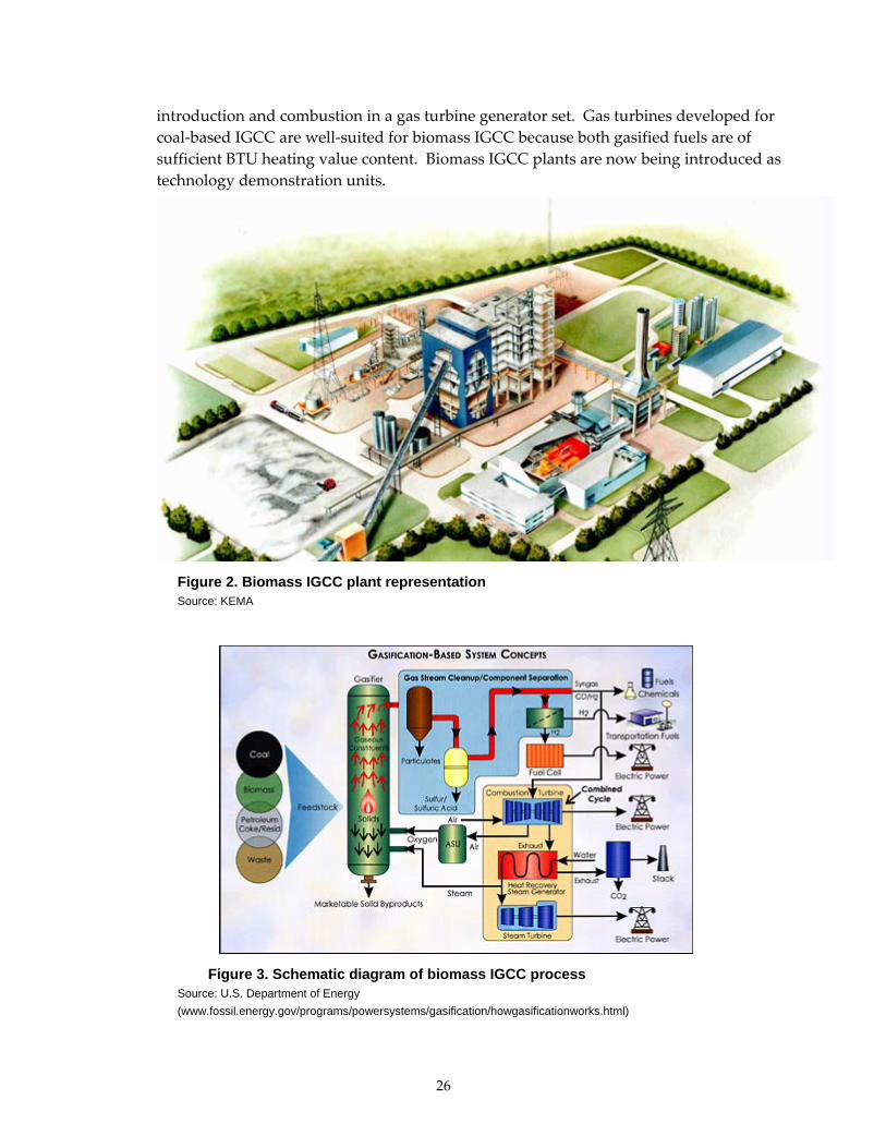
26
introduction and combustion in a gas turbine generator set. Gas turbines developed for coal‐based IGCC are well‐suited for biomass IGCC because both gasified fuels are of sufficient BTU heating value content. Biomass IGCC plants are now being introduced as technology demonstration units.
Figure 2. Biomass IGCC plant representation
Source: KEMA
Figure 3. Schematic diagram of biomass IGCC process
Source: U.S. Department of Energy (www.fossil.energy.gov/programs/powersystems/gasification/howgasificationworks.html)

27
• Biomass fluidized bed gasification – using a FB or CFB gasification reactor to convert biomass feedstocks into synthetic fuel gas, which is then burned in a conventional coal or natural gas‐fired utility boiler. This technology is not being adopted for the cost of generation study because the current commercial embodiment is direct fluidized bed combustion of biomass for electrical power generation.
Figure 4. Utility-scale biomass fluidized bed gasifier Source : Foster Wheeler
3.2.2. Biomass Combustion – Fluidized Bed Boiler Technical and Market Justification For biomass fuels, fluidized bed combustion is rapidly emerging as a system of choice for many power generation applications. The inherent fuel versatility of fluidized bed systems provides a plant operator the ability to burn many different biomass resource types, including those feedstocks with significant moisture variations. The major reason for this is that the fluidized bed carrying medium (typically a mix of silica sand and/or alumina) provides a thermal flywheel

28
effect that maintains constant heat output and flue gas quality even when burning fuels of varying moisture content.17
Fluidized bed boilers are characterized as either bubbling bed (FB) or circulating fluidized bed (CFB), and this is based on how the bed material is used within the boiler. In a bubbling bed (FB) unit, the bed material stays within a fixed zone in the boiler, while in a circulating fluidized bed (CFB) unit, the material is suspended above an air zone and is circulated through a return loop back to the combustion zone by means of a mass or cyclonic separator.
Figure 5. Circulating fluidized bed schematic diagram
Source: Babcock & Wilcox Image (www.babcock.com/products/boilers/images/cfb.gif)
For both FB and CFB units, due to the high quality combustion and near complete carbon burnout (99‐100%) of biomass fuel sources, ash is carried over into the flue gas stream, requiring the addition of post‐combustion ash removal equipment such as cyclones and baghouses. The
17 Overend, R.P. Biomass Conversion Technologies. Golden, CO: National Renewable Energy Laboratory, 2002.

29
post‐combustion controls allow particulate removal to New Source Performance Standards (NSPS) for PM10.
Fluidized bed boiler technology has long been in commercial use, with much more widespread adoption in Europe than in the United States, due to several reasons.18 First, fuel resources in Europe can vary widely in quality and processing, and the ability of fluidized bed boilers to handle widely varying fuels is of advantage. Second, fluidized bed boilers exhibit superior emissions performance, especially nitrogen oxide (NOx) emissions, due to the inherently low firing temperature of the boiler. Third, for coal‐based fuels, the ability to directly inject limestone as a sorbent provides excellent sulfur and sulfur dioxide (SOx) reductions without the need for expensive post‐combustion scrubbing equipment and systems.
Market adoption of fluidized bed boiler technology for biomass has long been a commercial reality, with both bubbling bed and CFB units being used for biomass cogeneration throughout the United States, particularly in the forest products and paper industry. Adoption of CFB technology for utility‐scale coal and biomass power generation has reached worldwide general industry adoption, as shown below:
Table 7. Installed CFB boiler capacity by country19
Country Installed Capacity (MW) China 10,000 Czech Republic 1,400 Germany 1,800 Poland 3,310 India 1,200 United States 8,800
Source: Tavoulareas, Stratos. Advanced Power Generation Technologies – An Overview
Technology Selection Criteria
Fluidized bed combustion technology for generating electric power using biomass fuel was selected for the cost of generation study by the research team because of the following factors:
• Commercial scale – Both bubbling bed and circulating fluidized bed technologies have been developed to utility scale, and current commercialized units fit well within the overall supply curve constraints for biomass that can limit overall generating unit size potential.
18 U.S. Environmental Protection Agency. Combined Heat and Power Partnership. Biomass Combined Heat and Power Catalog of Technologies, September 2007.
19 Tavoulareas, Stratos. Advanced Power Generation Technologies – An Overview. U.S. Agency for International Development. ECO‐Asia Clean Development Program, August 2008.

30
• Fuel flexibility – Biomass combustion in fluidized bed boilers has been well documented for a variety of biomass fuel feedstocks. The inherent stability in fluidized bed boilers while burning fuels of varying quality is a key advantage when evaluating changing biomass fuel sources over the life of the generating plant.
• Reliability – Fluidized bed combustion is reliable and proven over decades of service. While relatively new in technology when compared to stoker‐ or traditional‐fired boilers, there is rapid and growing adoption of fluidized bed boiler technology for mid‐sized units.
• Emissions performance – Fluidized bed combustion performs well in reducing NOx emissions because of the low combustion temperatures used in the process. In addition, the near‐complete conversion of available carbon results in lower carbon monoxide (CO) emissions. Particulate emissions are managed through post‐combustion controls, as with traditional‐fired units burning solid fuels.
Figure 6. Bubbling fluidized bed boiler
Source: Energy Products of Idaho

31
Primary Commercial Embodiment Today, the primary commercial embodiment of circulating fluidized bed boiler technology is in Europe and China and gaining momentum in the United States For over 20 years, the development of circulating and bubbling fluidized bed technology has progressed in Europe to the point where circulating fluidized bed boilers are a standard, utility‐scale technology today. In the United States, several companies have progressed with standardized designs of circulating fluidized bed boilers combusting a variety of fuels, from biomass to coal and petroleum coke.
In California, current commercial embodiment is limited, mainly because of the limited ability to permit solid‐fuel combustion facilities. However, there is current interest in the cogeneration and forest‐products industrial base to examine fluidized bed combustion technology for repowering existing solid‐fuel combustion facilities to biomass fuel conversion.20
The research team believes that fluidized bed technology will become commercially embodied in California to enable the state to achieve its biomass energy goals by 2018. The inherently fuel flexible nature of fluidized bed combustion, the integration of primary pollution controls into the combustion process, and the small footprint are enablers of this technology in California, as being demonstrated now in Europe and China.
Cost Drivers Market and Industry Changes
Market and industry changes since August 2007 have not significantly affected costs for circulating fluidized bed boiler technology. Material cost increases have abated due to the current economic recession, especially in carbon steel and stainless steel costs, which are the primary cost components of circulating fluidized bed boiler manufacturing.
Carbon steel costs have changed significantly since August 2007, but the net change is not significant. The attached table highlights the rapid rise and then fall of carbon steel pricing:21
Table 8. Recent carbon steel pricing
Year Average Carbon Steel Price ($/Ton) 2007 $717 2008 $1,004
2009 (April 2009 average annual price) $736 Source: Purchasing Magazine
20 KEMA Sources :Personal Communication with EPI, Foster Wheeler, March 2009.
21 Purchasing Staff. “Steel plate prices have plunged 50% from mid‐2008 peak.” Purchasing Magazine. April 2009. www.purchasing.com/article/CA6654110.html?industryid=48389.

32
Current Trends
Current trends that will materially affect future costs are:
• Global economic downturn – The breadth and depth of the current recession has caused a significant reduction in the number of new boiler orders for both power generation and industrial manufacturing capacity. The length of the current recession and the pace of recovery will determine the escalation rate in raw materials, the use of boiler manufacturing capacity, and thus future costs.
• Steel price abatement – Current amelioration of worldwide steel prices, both for carbon and stainless steel, will have a price‐moderating effect on stoker boiler prices both now and in the near future. Long‐term steel commodity prices are currently difficult to predict.
• Industrial production and economic growth in China – By November 2008, China lost over 30 million manufacturing jobs in Guangzhou Province due to the global recession, significantly curtailing Chinese economic gross domestic product (GDP) growth. Enough of the global output for steel and other raw materials, used in circulating fluidized bed boiler production, were being used in China that significant escalation of prices resulted. The pace of the economic recovery and stimulus in China will determine raw material price escalation and thus will impact circulating fluidized bed boiler costs.
• Economic stimulus –Because stimulus packages are designed to support energy technologies, such as combined heat and power, cogeneration, and biomass, stimulus support in the United States could have an escalating effect on both materials and demand for circulating fluidized bed boilers.
Cost Drivers
Cost drivers for biomass circulating fluidized bed boiler technologies are as follows:
• Biomass fuel type and uniformity – The type and uniformity of delivered biomass fuel supply is a primary cost driver for any biomass technology. Because of the varied nature of biomass fuel feedstocks, their delivered moisture content and heating value variations, and fuel processing issues, the handling and processing costs of biomass fuels can vary greatly. As a result, the type and nature of biomass fuels combusted can have a material impact on the capital cost of the boiler island design, as well as the overall fuel handling and operations cost.
• Supply curve for biomass fuel, fuel transport and handling costs – The availability of adequate and sufficient biomass fuel resources within a 100‐mile radius of the plant location is a critical driver for operating cost. Most biomass fuel is transported by truck transport to a plant site, which limits the effective economic radius from the plant location to aggregate fuel supply at commercially reasonable prices. The varied nature of biomass fuel feedstocks also necessitates special handling equipment and larger

33
numbers of dedicated staff than for coal‐fired combustion power plants of equivalent size.
• Boiler island cost – Capital cost of the boiler island is a critical cost driver that can entail approximately 40‐60% of the overall plant cost, depending on the type of biomass combusted and the need for post‐combustion pollution controls.22 The design basis for the type of fuels to be combusted is an important cost driver. In addition, the escalation trends for raw materials used in manufacture of the boiler island, primarily steel cost, are factors that can influence delivered boiler island cost.
• Long‐term fuel supply contract availability – Most current biomass fuel supply contracts are of short‐term duration and for fuel of sometimes varying quality. A key cost driver to promoting biomass circulating bed combustion in California is the ability to develop and achieve performance on long‐term (e.g., five years duration and longer) fuel supply contracts for available fuel sources.
• Plant scale – Current CFB technology has been proven to utility‐scale applications of up to 300 MW, with the primary commercial embodiment in sizes from 30‐100 MW. Development of 800 MW class supercritical CFB cycles is now being studied for applications in China, and the outcome of that research effort would materially affect the capital cost profile and scale of CFB technology applications for biomass.23
• Emissions control costs – Costs especially of post‐combustion emissions control technologies, such as SCR/SNCR technologies for NOx control, and additional particulate matter controls, are important cost drivers that can significantly increase the capital and operating costs of a commercial fluidized bed boiler combusting biomass.
• Retrofit versus greenfield/new site – For many biomass fluidized bed applications, repowering is a commercially viable option that can save 20‐40% of the capital cost of a new greenfield site where all balance‐of‐plant systems would need to be constructed.
• O&M capitalization – The extent to which the long‐term operations and maintenance of a biomass fluidized bed facility is capitalized through a long‐term maintenance contract with an OEM supplier is a cost driver. These long‐term maintenance contracts trade risk for maintenance cost predictability and can slightly change the operating cost profile of a commercial biomass fluidized bed boiler plant.
22 KEMA Sources: Personal Communication with Energy Products of Idaho, Coeur d’Alene, ID, March 2009.
23 Tavoulareas, Stratos. Advanced Power Generation Technologies – An Overview. U.S. Agency for International Development. ECO‐Asia Clean Development Program, August 2008.

34
Current Costs Current costs for biomass circulating fluidized bed boiler plants were primarily derived from three sources:
• Primary written research, reviewing the commercial embodiment of the technologies, and their instant and installed cost profiles.
• Research team direct communication with current technology manufacturers and developers of biomass CFB and bubbling bed plants.
• Research team direct experience in biomass and CFB plant development, construction, and operations, both in the United States and Europe.
The cost data gained through these three methods allowed for the comparison and contrast of capital and operating plant data and provided a detailed cost comparison for low/average/high cost case development.
Plant capacities for biomass fluidized bed boilers were established in a range of 15‐70 MW, with 28 MW being the average plant capacity. The capacity range is primarily set by the effective biomass fuel supply range, along with the commercial embodiment of most biomass CFB designs today.
Capacity factors were modeled in the range of 75‐90%, with 85% being the average value. These capacity factors are consistent with operational CFB boilers in commercial service.
Instant cost ranges for biomass CFB plants ranged from a low case of $1,600 per kilowatt (kW) to a high case of $4,800/kW, with an average CFB plant cost of $3,200/kW. These instant costs can vary widely due to a number of factors: type of fuel and fuel mix burned, size/scale of the plant, whether the site is a brownfield redevelopment or a greenfield site, and the amount of post‐combustion pollution controls needed to satisfy air quality and permitting requirements. Typically, the boiler island comprises 40‐60% of the total instant plant cost.
Heat rates are similar to those of other solid‐fuel technologies, ranging from 9,800 British thermal units (Btu) per kilowatthour (kWh) to 11,000 Btu/kWh, with 11,500 Btu/kWh being used as the average. Heat rates can vary for biomass CFB systems due to fuel moisture content and heating value.
Expected Cost Trajectories Cost trajectories for biomass fluidized bed boiler technology were developed through examination of several factors.
Capital cost and installation duration for a fluidized bed plant provide the largest trajectory difference. In all cases, the research team assumed a biomass fluidized bed plant is developed by a merchant generator, as there are few applications worldwide that have been developed for cogeneration purposes, either in the forest/paper industries, the MSW industries, or for

35
enhanced oil/gas recovery.24 Construction periods were set for either a two or three‐year construction cycle, mostly dependent on permitting approvals and receipt of air quality approvals.
Determination of installed costs were derived from examining interest costs during construction, plus the range in expected construction costs for the low, average, and high cases.
No significant experience curve effects or learning effects are taken into consideration in the analysis, as CFB technology is considered a mature technology. Cost drivers should not have a significant impact on the long‐term levelized cost values, absent a disruptive shift in the current technology and approach to biomass CFB combustion.
3.2.3. Biomass Combustion – Stoker Boiler Technical and Market Justification Stoker boilers have been used for solid fuel combustion and power generation for over a century. Generally used for small‐scale power generation under 100 MW in size, the primary stoker boiler technology types for biomass are moving grate and encompass traveling grate, vibrating grate, and spreader stoker variants of the technology.
Figure 7. Stoker boiler schematic diagram Source: Boilermech, (www.boilermech.com)
24 California Biomass Collaborative. California Biomass Facilities Reporting System, March 2009. http://biomass.ucdavis.edu/tools.html.

36
Biomass‐fired stoker boiler technology has evolved to provide reliable, efficient combustion and energy generation. Today, modern biomass stoker combustion systems provide an efficient, stable combustion process while supplying the desired boiler heat input with low emissions:
• Efficient combustion – Produces efficient use of the biomass feedstock fuel supply through burning with low carbon monoxide (CO) emissions and low unburned carbon (UBC), which is an indicator of combustion efficiency.
• Stable combustion – Produces stable and consistent combustion to maintain consistent design parameters and boiler performance, even with changing biomass fuel supply mix.
• Heat input – Generates the heat input to support the power generation cycle.
• Low emissions – Produces low carbon monoxide, low unburned carbon (UBC), and low nitrogen oxides (NOx).25
Modern stoker designs have improved significantly over vintage boilers installed pre‐1965, when the majority of commercial stoker boilers were installed.26 Today’s biomass stoker boilers have improvements that enhance their ability to burn biomass feedstocks of varying quality and type:
• Improved fuel feed controls and distribution of biomass across the grate – Provide more uniform heat release in the boiler, improving consistency and reliability of operation.
• Improved combustion air distribution – Improves efficiency and emissions performance, particularly NOx and CO emissions.
• Advanced overfire air systems – Complete combustion, improving efficiency and emissions performance and reduces unburned carbon and char when burning biomass fuels.
• Reduced excess air requirements – Improve combustion efficiency.
• Improved fuel/air mixing through better furnace gas path design and use of grate oscillation – Improves efficiency and reliability of furnace parts.25
25 Abrams, Richard F. and Kevin Toupin. “Efficient and Low Emission Stoker Fired Biomass Boiler Technology in Today’s Marketplace.” POWER‐GEN Renewable Conference Technical Publication, March 2007.
26 Gas Research Institute (GRI). Analysis of the Industrial Boiler Population. Energy and Environmental Analysis, Inc., June 1996.

37
Figure 8. Flow schematic for a stoker boiler configuration Source: DeFusco, McKenzie and Fick, “Bubbling Fluidized Bed or Stoker.” 27
Primary Commercial Embodiment Currently, California has approximately 30 solid‐fuel biomass facilities in the state, totaling 640 MW of generation. The vast majority of these plants are stoker boilers, installed in the 1970s and 1980s after the Public Utility Regulatory Policies Act (PURPA) came into effect, and serve primarily the forest products, pulp and paper, and waste‐to‐energy cogeneration markets. These plants operate reliably and effectively, although California has seen a decline in the number of solid‐fuel biomass plants due to two reasons: cost of biomass fuel supplies and more stringent emissions legislation in the state.
The primary commercial embodiment of the stoker boiler technology is not expected to change significantly by 2018, but the research team expects continuing improvements in fuel combustion technology to reduce emissions and increase fuel flexibility. In addition, the research team found improved post‐combustion emissions controls, such as selective catalytic reduction (SCR), and Riley’s selective catalytic reduction (RSCR™) – a combination of a regenerative thermal oxidizer and SCR. RSCR technology is significantly more thermally efficient than standard SCR technologies, providing NOx removal at much lower annual fuel costs.28
27 DeFusco, John, Phillip McKenzie, and Michael Fick. “Bubbling Fluidized Bed or Stoker – Which is the Right Choice for Your Renewable Energy Project.” CIBO Fluid Bed Combustion XX Conference, May 2007.
28 Abrams, Richard F. and Kevin Toupin . “Efficient and Low Emission Stoker Fired Biomass Boiler Technology in Today’s Marketplace.” POWER‐GEN Renewable Conference Technical Publication, March 2007.

38
Cost Drivers Market and Industry Changes
Market and industry changes since August 2007 have not significantly affected costs for stoker boiler technology. Material cost increases have abated due to the current economic recession, especially in carbon steel and stainless steel costs, which are the primary cost components of stoker boiler manufacturing.
Carbon steel costs have changed significantly since August 2007, but the net change is not significant. The attached table highlights the rapid rise and then fall of carbon steel pricing:29
Table 9. Recent carbon steel pricing
Year Average Carbon Steel Price ($/Ton) 2007 $717 2008 $1,004
2009 (April 2009 average annual price) $736 Source: Purchasing Magazine
Current Trends
Current trends that will materially affect future costs are:
• Global economic downturn – The breadth and depth of the current recession has caused a significant reduction in the number of new boiler orders for both power generation and industrial manufacturing capacity. The length of the current recession and the pace of recovery will determine the escalation rate in raw materials, the use of boiler manufacturing capacity, and thus future costs.
• Steel price abatement – Current amelioration of worldwide steel prices, both for carbon and stainless steel, will have a price‐moderating effect on stoker boiler prices both now and in the near future. Long‐term steel commodity prices are currently difficult to predict.
• Industrial production and economic growth in China – By November 2008, China lost over 30 million manufacturing jobs in Guangzhou Province due to the global recession, significantly curtailing Chinese economic gross domestic product (GDP) growth. Enough of the global output for steel and other raw materials used in stoker boiler production was being used in China that significant escalation of prices resulted. The pace of the economic recovery and stimulus in China will determine raw material price escalation and thus will impact stoker boiler costs.
• Economic stimulus – Because stimulus packages are designed to support energy technologies such as combined heat and power, cogeneration, and biomass, stimulus
29 Purchasing Magazine Staff. “Steel Plate Prices Have Plunged 50% From Mid‐2008 Peak.” Purchasing Magazine, April 2009. www.purchasing.com/article/CA6654110.html?industryid=48389.

39
support in the United States could have an escalating effect on both materials and demand for stoker boilers.
Cost Drivers
Cost drivers for stoker‐fired biomass combustion boiler plants are as follows:
• Biomass fuel type and uniformity – The type and uniformity of delivered biomass fuel supply is a primary cost driver for any biomass technology. Because of the varied nature of biomass fuel feedstocks, their delivered moisture content and heating value variations, and fuel processing issues, the handling and processing costs of biomass fuels can vary greatly. As a result, the type and nature of biomass fuels combusted can have a material impact on the capital cost of the boiler island design, as well as the overall fuel handling and operations cost.
• Supply curve for biomass fuel, fuel transport, and handling costs – The availability of adequate and sufficient biomass fuel resources within a 100‐mile radius of the plant location is a critical driver for operating cost. Most biomass fuel is transported by truck transport to a plant site, which limits the effective economic radius from the plant location to aggregate fuel supply at commercially reasonable prices. The varied nature of biomass fuel feedstocks also necessitates special handling equipment and larger numbers of dedicated staff than for coal‐fired combustion power plants of equivalent size.
• Boiler island cost – Capital cost of the boiler island is a critical cost driver that can entail approximately 40‐60% of the overall plant cost, depending on the type of biomass combusted and the need for post‐combustion pollution controls.30 The design basis for the type of fuels to be combusted is an important cost driver. In addition, the escalation trends for raw materials used in manufacture of the boiler island, primarily steel cost, are factors that can influence delivered boiler island cost.
• Long‐term fuel supply contract availability – Most current biomass fuel supply contracts are of short‐term duration and for fuel of sometimes varying quality. A key cost driver to promoting biomass combustion in California is the ability to develop and achieve performance on long‐term (e.g., five years duration and longer) fuel supply contracts for available fuel sources.
• Emissions control costs – Costs especially of emissions control technologies, such as advanced overfire air or SCR/SNCR technologies for NOx control and additional
30 KEMA Sources: Personal Communication with Energy Products of Idaho, Coeur d’Alene, ID, March 2009.

40
particulate matter controls, are important cost drivers that can significantly change the capital and operating costs of a commercial stoker boiler combusting biomass.31
• Retrofit versus greenfield/new site – For many biomass fluidized bed applications, repowering is a commercially viable option that can save 20‐40% of the capital cost of a new greenfield site where all balance‐of‐plant systems would need to be constructed.
Current Costs Current cost profiles for stoker boiler biomass combustion technology were developed using three primary research methods:
• Primary written research, reviewing the commercial embodiment of the technologies and their instant and installed cost profiles.
• Research team direct communication with current technology manufacturers and developers of biomass‐fired stoker boiler plants.
• Research team direct experience in biomass stoker combustion plant development, construction, and operations, specifically referencing a stoker boiler biomass plant in St. Paul, Minnesota.
Stoker‐boiler technology is considered a mature technology, with stoker designs having changed little in basic design or cost profile over a period of 40 years. Most of the design innovation being performed today in stoker technology is to upgrade the performance of stoker boilers to combust a wide range of biomass fuels (formerly, biomass fuels being combusted in a stoker boiler had to be relatively uniform in type and heat/moisture content), and to improve emissions control performance.32
Capital costs and sizes for stoker boilers were developed through direct communication with manufacturers, including Riley and Energy Products of Idaho. In addition, these costs were verified and contrasted with the Biomass Combined Heat and Power Catalog of Technologies reference document, compiled by the U.S. Environmental Protection Agency (EPA) Combined Heat and Power Partnership.33
Net capacity factors for stoker boilers can vary depending on the type of fuel source used, the variation in the fuel, and operating requirements of the plant. In general, stoker boilers burning
31 Abrams, Richard F. and Kevin Toupin . “Efficient and Low Emission Stoker Fired Biomass Boiler Technology in Today’s Marketplace.” POWER‐GEN Renewable Conference Technical Publication, March 2007.
32 Power Engineering, “Efficient and Low Emission Stoker‐Fired Biomass Boiler Technology in Today’s Marketplace.” Power Engineering, March 2007.
33 U.S. Environmental Protection Agency. Combined Heat and Power Partnership. Biomass Combined Heat and Power Catalog of Technologies, September 2007.

41
biomass have fewer capacity factors than if the boilers were using coal as fuel, with the primary reason being the larger variation in biomass fuel properties going to the stoker grate and the variation of the biomass fuel source over time. Capacity factors of 75%, 85%, and 90% were used based on fleet experience for the high‐cost, average‐cost, and low‐cost cases, respectively.
Plant capital cost data was examined through the construction of an average sized 38 MW plant, and scaled accordingly for the high and low‐cost cases, based on experience and actual plant data. For the low‐cost case, reference data from a prior retrofit site was used, and for the high cost case, scaling factors from manufacturers detailing the range in cost estimates were used.34
Plant heat rates were modeled using an average 40‐50% moisture woody biomass fuel feedstock and current stoker technology. Heat rate ranges are from 10,250 – 13,000 Btu/kWh, with an average heat rate of 11,000 Btu/kWh modeled. The research team notes that performance, ultimate capacity, and heat rate are strongly dependent on the biomass fuel type selected, its variation in combustion and moisture properties over time, and the mixing of biomass fuel sources. Moisture, for instance, is a key variable in determining biomass stoker performance because the energy used in heating and vaporizing the moisture content in the fuel is not recovered fully and thus negatively impacts overall performance.
Expected Cost Trajectories Cost trajectories for biomass stoker boiler technology were developed through examination of several factors.
Capital cost and installation duration for a stoker plant provides the first and largest trajectory difference. In all cases, the research team assumed a biomass stoker plant, developed by a merchant generator, as the vast majority of stoker applications are developed for cogeneration purposes in California, either in the forest/paper industries, the MSW industries, or for enhanced oil/gas recovery.35 Construction periods were set for either a two‐ or three‐year construction cycle, mostly dependent on permitting approvals and receipt of air quality approvals.
Determination of installed costs were found through the interest costs during construction, plus the range in expected construction costs for the low, average, and high cases. Expected installed costs for 2009 for the low, average, and high cases are:
Table 10. Biomass stoker installed cost ranges – 2009 dollars per kW installed
Low Case Average Case High Case $ 1,914 /kW $ 2,909 /kW $4,050/kW
Source: KEMA
34 KEMA Communication with Energy Products of Idaho, and direct experience with Market Street Energy project, St. Paul, MN, March 2009.
35 California Biomass Collaborative. California Biomass Facilities Reporting System, March 2009 (http://biomass.ucdavis.edu/tools.html).

42
Very little experience curve learning effects were modeled in the expected cost trajectories. The U.S. Department of Energy shows stoker combustion technology as a very mature technology and with little incremental improvement foreseen through 2030.36 A maximum learning rate of 5% through 2030 was modeled, along with a low‐case rate reflecting no learning through 2030 was modeled for the high case.
3.2.4. Biomass Cofiring Technical and Market Justification One of the most attractive and easily implemented renewable energy sources is derived from cofiring of biomass in existing coal fired boilers. In biomass cofiring, up to 20%‐30% of the coal can be displaced by biomass. The biomass and coal are combusted simultaneously. The term biomass refers to materials derived from plant matter such as trees, grasses, and agricultural crops. These materials, grown using energy from sunlight, can be renewable energy sources for fueling many of today’s energy needs. Cofiring projects replace a portion of the nonrenewable fuel–coal–with a renewable fuel–biomass.
Figure 9. Biomass cofiring schematic for a pulverized coal boiler system Source: U. S. Department of Energy, Energy Efficiency and Renewable Energy
36 U.S. Department of Energy. Energy Information Administration. Office of Integrated Analysis and Forecasting. Learning Parameters for New Generation Technology Components.

43
When it is used as a supplemental fuel in an existing coal boiler, biomass can provide the following benefits: lower fuel costs, more fuel flexibility, avoidance of waste to landfills and their associated costs, and reductions in sulfur oxide, nitrogen oxide, and greenhouse gas emissions. Other benefits such as decreases in flue gas opacity have also been documented.
Cofiring is a proven technology. Over the past 15 years, the research team has found extensive experience with direct and indirect cofiring of several types of biomass fuels. KEMA has tested cofiring mixtures of coal and several biomass fuels up to about 25% (on an energy basis) in KEMA’s 1 MW test boiler and has been involved in over 50 full‐scale commercial and demonstration projects in coal‐fired power plants. In addition, many utilities have cofiring biomass in coal‐fired generation plants, as noted in the following table:37
Table 11. Coal-fired generation plants with biomass cofiring
Facility Name Company City/County State Capacity (MW)
Heat Input from Biomass (Percent of
Total) 6th Street Alliant Energy Cedar Rapids IA 85 7.7 Bay Front Xcel Energy Ashland WI 76 40.3 Colbert TVA Tuscumbia AL 190 1.5 Gadsden 2 Alabama
Power Gadsden AL 70 <1.0
Greenridge AES Dresden NY 161 6.8 C.D. Mcintosh, Jr. City of
Lakeland Polk FL 350 <1.0
Tacoma Steam Plant
Tacoma Public Utilities
Tacoma WA 35 44.0
Willow Island 2 Allegheny Power
Pleasants WV 188 1.2
Yates 6 and 7 Georgia Power Newnan GA 150 <1.0 Source: Haq, Zia. Biomass for Electricity Generation
The Electric Power Research Institute (EPRI) began research and testing of biomass cofiring in utility boilers in 1992, and with success cofiring biomass percentages of up to 40% of fuel requirements. In Europe, the Netherlands has undertaken extensive studies of biomass cofiring of up to 30% of boiler fuel requirements. Biomass cofiring is currently a valid commercial technology for coal‐fired utility‐scale power plants, having been tested in a wide range of boiler types, including cyclone, stoker, pulverized coal, and fluidized bed boilers.38
37 Haq, Zia, Biomass for Electricity Generation. U.S. Department of Energy. Energy Information Administration, 2002.
38 U.S. Environmental Protection Agency. Combined Heat and Power Partnership. Biomass Combined Heat and Power Catalog of Technologies, September 2007.

44
Biomass cofiring technology is versatile and can be accomplished in several ways, depending on the percentage of biomass to be cofired with coal, and the design of the specific boiler system. In general, there are four main routes to successfully accomplish cofiring, as shown in the diagram below:
• Co‐milling of biomass with coal.
• Separate milling, injection in pf‐lines, combustion in coal burners.
• Separate milling, combustion in dedicated biomass burners.
• Biomass gasification, syngas combusted in furnace boiler.
Mills Coal
Biomass
Steam Turbine
Flue Gas Treatment
Boiler Burners
Pre- treatment
Stack Gasifier
Mills
2 31
4
Figure 10. Primary biomass cofiring locations Source: KEMA, Inc.
Co‐milling of biomass with coal, and separate milling and injection/combustion into the coal burners are the most common route for biomass cofiring when the overall percentage of biomass to coal is relatively small (<15%). In these applications, the biomass blends well with a predominantly coal mixture, and is combusted in the boiler with little operational impact.
For larger percentages of cofiring with biomass, typical applications will require the addition of separate feed streams of the biomass, along with the addition of dedicated biomass burners. These boiler modifications are needed because of the differing characteristics and heating values of the fuel (biomass – 9000 Btu/lb, versus coal – 12,000 Btu/lb), and the varying feedstock quality that can often be found in biomass fuel supply.
In addition, a fourth route to cofiring biomass is to gasify it, usually in a fluidized bed gasifier, and then combust the synthetic gas in the furnace with dedicated gas burners. This approach is increasingly gaining market acceptance, particularly with the successful commercial operation

45
of fluidized bed gasifiers, and is a driving technology behind the retrofit of older technology biomass stoker plants.39
Primary Commercial Embodiment The primary commercial embodiment of biomass cofiring technology in California is found in two forms:
• Addition of biomass cofiring to the small number of remaining utility‐scale coal boilers in California, typically up to 30% cofiring. In addition, biomass cofiring is feasible in the WECC region coal‐fired plants that currently export generation and energy to California.
• Addition of biomass cofiring to the existing small utility‐scale coal boilers in operation (20‐50 MW), of which there are approximately 30 plants that currently exist, and approximately 66 plants feasible if currently closed biomass facilities are repowered.
By 2018, the primary commercial embodiment is predicted by the research team to be similar to the current state, with incremental operating improvements gained by additional cofiring experience. The research team notes that several companies are looking at their current biomass cofiring experience to be an interim step towards complete fuel switching from coal to 100% biomass fuel, as climate change legislation appears more likely before 2018.
Cost Drivers Market and Industry Changes
Since August, 2007, there has been additional industry experience with cofiring biomass due to emissions legislation in the United States, plus continued emphasis on biomass cofiring implementation in the European Union. These industry changes have helped cofiring gain additional momentum as a useful generation technology addition for carbon reduction and climate change mitigation strategies. As of this report, these industry changes have not had a discernable impact on market prices for cofiring adoption.
Current Trends
Currently, biomass cofiring is one of the most inexpensive ways to increase use of biomass feedstocks and fuel sources. Requiring only a fraction of the investment capital for new plant, the research team believes it is a technology with significant potential to help biomass become competitive in the energy landscape.
Cost Drivers
Cost drivers for biomass circulating fluidized bed boiler technologies are as follows:
39 Energy Products of Idaho, Cœur d’Alene, ID.

46
• Biomass fuel type and uniformity – The type and uniformity of delivered biomass fuel supply is a primary cost driver for any biomass technology. Because of the varied nature of biomass fuel feedstocks, their delivered moisture content and heating value variations, and fuel processing issues, the handling and processing costs of biomass fuels can vary greatly. As a result, the type and nature of biomass fuels combusted can have a material impact on the capital cost of the boiler cofiring upgrades, as well as the overall fuel handling and operations cost. For biomass cofiring, the amount of biomass cofiring and uniformity of the fuel can affect the operating combustion and temperature profiles in the boiler, and thus the overall cost of boiler improvements.40
• Supply curve for biomass fuel, fuel transport, and handling costs – The availability of adequate and sufficient biomass fuel resources within a 100‐mile radius of the plant location is a critical driver for operating cost. Most biomass fuel is transported by truck to a plant site, which limits the effective economic radius from the plant location to aggregate fuel supply at commercially reasonable prices. The varied nature of biomass fuel feedstocks also necessitates special handling equipment and larger numbers of fuel handling personnel than for a similarly sized coal‐fired plant.
• Boiler island capital upgrade cost – Capital cost of necessary boiler modifications, depending on the cofiring fuel injection point is a critical cost driver that can entail approximately 50% of the overall capital upgrade cost, depending on the type of biomass combusted and the location of the biomass cofiring injection point.41 In addition, the escalation trends for raw materials used in manufacture of the boiler fuel feed and pressure parts, primarily steel cost, are factors that can influence the final installed cost of cofiring upgrades to the boiler.
• Long‐term fuel supply contract availability – Most current biomass fuel supply contracts are of short‐term duration and for fuel of sometimes varying quality. The ability to write and achieve performance on long‐term (e.g., five years duration and longer) fuel supply contracts for available fuel sources is a key cost driver to securing additional biomass cofiring generation.
• O&M capitalization – The extent to which the long‐term operations and maintenance of boiler upgrades required to support a high (>10% biomass cofiring) level of biomass cofiring is capitalized through a long‐term maintenance contract with an OEM supplier is a cost driver. These long‐term maintenance contracts trade risk for maintenance cost predictability, and can slightly change the operating cost profile of a commercial boiler plant cofiring both coal and biomass fuels.
40 Dayton David, A Summary of NOx Emissions Reduction From Biomass Cofiring. National Renewable Energy Laboratory, May 2002.
41 KEMA Sources: Personal Communication with Energy Products of Idaho, Coeur d’Alene, ID, March 2009.

47
Current Costs Current costs were developed by examining the biomass cofiring technology within the context of operation of current coal‐fired utility‐scale boiler technology, coupled with the experience base of cofiring biomass both in Europe and in the United States. Plant scale was developed by using the 5‐30% general cofiring ranges seen in current applications, and especially those successfully demonstrated in the United States.42 Capacities used in the model ranged from 10 ‐40 MW gross capacity due to biomass cofiring, and incremental to the nominal coal‐fired output of the boiler plant.
Capacity factors modeled were from 85‐95%, reflecting current test burn and operational experience showing that there is not a detrimental availability impact caused by cofiring biomass within the nominal 5‐30% ranges.
Efficiency and heat rate ranges were also chosen based on nominal increases to heat rate due to moisture content of the fuel, but otherwise tracked current coal‐plant industry heat rates. Heat rate ranged from 9,800 Btu/kWh to 12,000 Btu/kWh, with an average heat rate modeled at 10,500 Btu/kWh.
Capital requirements for the cofiring technology were based on both current industry experience combined with the research team experience base in cofiring biomass in the Netherlands. Instant (overnight) capital cost ranges were modeled between 400 – 700 $/kW, with an average of $500/kW. All boiler modifications for cofiring technology are assumed to be constructed within one year.
Expected Cost Trajectories The type of boiler modifications and technologies involved in biomass cofiring are extremely mature technologies involving burner modifications, injection point rework, and fuel handling systems. Based on the maturity of these technologies, very little experience curve effects are anticipated, and only small incremental improvements in cost performance are foreseen by the research team. A technology progress ratio for biomass cofiring of 0.990 was assigned to this technology based on the similarities of cofiring technologies to established solid‐fuel cofiring and test burn technology applications. The progress ratio indicates that, with a doubling of the installed biomass cofiring capacity, one would expect a 1% improvement in cost performance over time.
The overall cost performance of biomass cofiring technologies is expected to track the rate of inflation over the long run.
3.2.5. Biomass Co-Gasification IGCC Technical and Market Justification Biomass co‐gasification IGCC is a unique technology that has many commercial utility‐scale applications. Biomass IGCC draws upon the technology base used to develop and
42 Blume, Grant, Ronald Meijer, and Kevin Sullivan, “Cofiring of Biomass in the US.” Renewable Energy World Conference Presentation, March 2009.

48
commercialize coal‐based IGCC plants beginning with the first commercial scale utility unit at Duke Energy’s Wabash River Generating Station in 1995. Since that time, both coal and biomass‐based IGCC has been commercialized as a viable generating technology, with key advantages:
• Feedstock flexibility – Because the combined‐cycle unit is fired with synthetic gas from the gasifier units, a variety of fuel feedstocks, from coal to petroleum coke and biomass, can be used.
• Low emissions – Similar to a natural gas‐fired combined‐cycle unit and much lower than solid‐fueled coal units.
• Carbon capture – IGCC cycles are particularly suitable for carbon capture and sequestration, since carbon dioxide is emitted in separate streams that may be captured and disposed in a normal process cycle.
The key approach to the IGCC cycle application for biomass fuels is the ability of current generation gas turbines to accept and burn low‐BTU content gas streams. This technology shift has happened over the last 15 years, and now most modern gas turbine engines will combust biomass‐based syngas in turbine size ranges suitable for most biomass development plant scales.43
The first successful demonstration project for biomass co‐gasification IGCC was in Varnamo, Sweden, and ran from 1992 through 2000 at 18 MW combined heat and power output.44
As of 2007, the biomass gasification market counted 13 active biomass gasifiers from companies worldwide, encompassing four major technology types:45
• Atmospheric pressure circulating fluidized bed gasifier – In commercial operation at Lahti, Finland, producing 42 MWe since 1998, and using biofuels, RDF (refuse derived fuel), and wood waste as biomass feedstocks.
• Pressurized circulating fluidized bed gasifier (PCFB) – Demonstrated at Varnamo, Sweden, through 2000, and producing 6 MWe using wood, RDF and straw as biomass feedstocks.
• Plasma gasifier – Demonstrated at Utashinai, Japan, in 2003, producing 8 MWe in commercial operation, using a downward moving bed and plasma bottom torch.
43 Overend, Ralph P. Biomass Conversion Technologies. Golden, CO: National Renewable Energy Laboratory, March 2002.
44 Stahl, Krister, Lars Waldheim, Michael Morris, Ulf Johnsson, and Lennart Gårdmark. “Biomass IGCC at Varnamo, Sweden – Past and Future.” GCEP Energy Workshop, April 2004.
45 Cobb, James T. “Survey of Commercial Biomass Gasifiers.” University of Pittsburgh, AIChE Annual Meeting, November 2007.

49
• Draft type – original technology, and not generally suitable for gas turbine applications because of tar carryover.
Figure 11. Process flow diagram for biomass gasification and conditioning for IGCC application Source: Rhodes and Keith, “Engineering economic analysis of biomass IGCC.” 46
Primary Commercial Embodiment Currently, there is no primary commercial embodiment in California, as the use of biomass IGCC has not yet been commercialized. However, the basic premise of coal‐based IGCC is a commercial technology, and in the United States, utility‐scale coal‐based IGCC plants are being developed with the capability to cofire biomass feedstocks in limited percentages (<15%).
By 2018, the research team expects the biomass IGCC technology to become commercialized, with CFB gasifier technology as the leading approach for biomass IGCC development.
46 Rhodes, James S. and David W. Keith. “Engineering Economic Analysis of Biomass IGCC With Carbon Capture and Storage.” Biomass and Bioenergy 29 (2005): 440‐450.

50
Cost Drivers Market and Industry Changes
Market and industry changes since August 2007 have favored the rapid development of utility‐scale biomass IGCC plants. The first change in the market is pending climate change legislation that will impose a cap‐and‐trade system for carbon dioxide and other GHG emissions. This change will drive technology development to those approaches that can capture and sequester carbon, as well as carbon‐neutral approaches to power generation. Biomass IGCC, because of the near‐zero carbon emission profile of biomass fuels, coupled with the ability to capture carbon dioxide, is an ideal technology for a carbon‐constrained power generation market.
Second, the increased deployment of coal‐fired IGCC units, such as the recently announced repowering project at Duke Energy’s Edwardsport station in Indiana, will further the development of gasification reactor technology. Gasifier trains will be tested and technology developed to reliably gasify biomass feedstocks along with coal.
Third, active research in biomass gasification and co‐gasification with coal is being conducted in Europe, particularly in the Netherlands, where biomass co‐gasification experiments of up to 50% biomass by weight are being conducted at two power stations.47
Current Trends
Future costs for biomass co‐gasification will be driven by the development of commercial gasifier trains that are able to handle wide variations in biomass feedstock materials. As these technologies become more mature, experience effects will drive down the overall capital cost of these plants.
Cost drivers for biomass integrated gasification combined‐cycle plant technologies are as follows:
• Biomass fuel type and uniformity – The type and uniformity of delivered biomass fuel supply are primary cost drivers for any biomass technology. Because of the varied nature of biomass fuel feedstocks, their delivered moisture content and heating value variations, and fuel processing issues, the handling and processing costs of biomass fuels can vary greatly. As a result, the type and nature of biomass fuels combusted can have a material impact on the capital cost of the fuel handling systems and the gasifier process trains. Fuel variability in the gasification process can alter process properties, and result in changes to the required gasifier size.48
• Supply curve for biomass fuel, fuel transport and handling costs – The availability of adequate and sufficient biomass fuel resources within a 100‐mile radius of the plant location is a critical driver for operating cost. Most biomass fuel is transported by truck
47 KEMA sources and research.
48 Murphy Michael, Repowering Options: Retrofit of Coal‐Fired Boilers With Fluidized Bed Biomass Gasification. Energy Products of Idaho, 2001.

51
to a plant site, which limits the effective economic radius from the plant location to aggregate fuel supply at commercially reasonable prices. The varied nature of biomass fuel feedstocks also necessitates special handling equipment and larger numbers of fuel handling personnel than for a similarly sized coal‐fired plant.
• Boiler/gasifier capital costs and trajectory – The primary driver in determining overall costs is the capital costs and long‐run cost trajectories for the gasifier trains required to gasify biomass fuel feedstocks. After several decades of commercial development and embodiment of the technology in coal‐gasification applications, the technology is considered relatively mature, and few scale effects are anticipated. In addition, the escalation trends for raw materials used in manufacture of the gasifier plant, primarily steel and alloy steel cost, are factors that can influence the final installed cost of installing biomass gasification technology.
• Long‐term fuel supply contract availability – Most current biomass fuel supply contracts are of short‐term duration and for fuel of sometimes varying quality. The ability to write and achieve performance on long‐term (e.g. five years duration and longer) fuel supply contracts for available fuel sources is a key cost driver to securing financing for more expensive biomass gasification projects.
Current Costs Gross capacity ranges between 25‐40 MW were modeled for biomass gasification combined‐cycle units, primarily reflecting the effective size range and fuel supply radius for sourcing biomass fuel feedstocks. These ranges also embody current project sizes now under development in California, though not yet built, and they also fall readily within currently available fluidized bed gasification technologies.
Net capacity factors are modeled as between 65‐80%, reflecting the on‐stream expected times of gasifier train units processing biomass fuel, coupled with the expected availability of the gas turbine combined‐cycle generation units.
Instant costs were modeled based on direct conversations with active developers reviewing projects in California, combined with industry costs for fluidized bed gasifier trains supporting between 25‐40 MW class plants, and existing industry combustion turbine combined‐cycle data. These costs in total average $2,950/kW, with a high range of $3,688/kW and a low range of $2,655/kW modeled. High case costs reflect additional capital cost for biomass fuel variation characteristics, and low case costs reflect simpler fuel processing and handling costs.
Construction durations for total installed cost calculations range from one to three years duration, with the average plant constructed within a two‐year time horizon.
Plant efficiency and heat rate were modeled based on the overall expected performance of the gas turbine combined‐cycle coupled with the gasifier train operating as a fluidized bed unit. Overall heat rates between 10,000 – 11,000 Btu/kWh were modeled by the research team, with an average expected heat rate of 10,500 Btu/kWh.

52
Expected Cost Trajectories Expected cost trajectories for biomass IGCC development will track closely the technology progress for coal‐based integrated gasification technologies. Those technologies are considered mature after over two decades of commercial development and embodiment, and significant experience curve effects are not anticipated to reduce overall installed cost base.
The research team used a modified technology progress ratio range of 0.98 to 1.00 to model biomass integrated gasification combined‐cycle experience curve trajectories, as this technology has matured in the coal‐based environment in which it has developed. Some sources characterize additional learning curve effects with the gasifier train development, of up to a 10% learning curve improvement in the period after 2020, but the research team did not incorporate this view into the analysis for cost trajectory development.49 The rationale is that the expected embodiment of this technology in California will be primarily bubbling and circulating fluidized bed gasifier trains, and this technology is well‐established for gasifying biomass fuels. Other technologies currently under development for coal fuel feedstocks would need additional development to handle the widely varying characteristics common to biomass, and this resulted in a selection of a more conservative learning rate for this technology by the research team.
3.3. Geothermal 3.3.1. Technology Overview Geothermal energy is derived from heat from beneath the Earth’s surface that flows to the surface through a variety of pathways from hot water, steam reservoirs, or heated rock formations. Heat is carried continuously upward to the Earth’s surface as steam or hot water when water flows through permeable rock. California has the largest geothermal megawatt production and potential of any state. Currently, only a fraction of California’s enormous geothermal resources are used. Approximately 94% of all known United States hydrothermal resources are located in California.
Currently in the United States, geothermal energy accounts for approximately 2,850 megawatts of electric power, enough electricity for 3.7 million people. The cost of producing this power ranges from 4 to 8 cents per kWh. The nationʹs electrical power generation was estimated at 80 quadrillion Btu (quads) in 1990. Of this amount, renewable energy produced 6.4 quads in 1990 or 8% of the nationʹs total energy consumption. It is estimated that renewable energy sources have the potential to supply as much as 36.6 quads by 2030. Geothermal resources are predicted to be the largest short‐term supplier of renewable electric power, with more than a tenfold increase or 3.3 quads projected by 2010. This is approximately 35% of the calculated renewable energy contribution.
49 U.S. Department of Energy. Energy Information Administration. Learning Curve Effects for New Technologies.

53
Types of Geothermal Resources Most geothermal resources fall into one of the following categories: vapor‐dominated, liquid‐dominated, geopressure, hot dry rock, and magma. Geothermal resources result from a concentration of the Earthʹs thermal energy within regions of the four subsurface types. Of these resources, only vapor‐ and liquid‐dominated resources have been developed commercially for power generation.
Vapor-Dominated Resources Vapor‐dominated resources contain superheated steam above 200°C (382°F) and are rare in nature. The resources have been proven to be economical to exploit for electricity generation. In California the only vapor‐dominated resource, known as The Geysers, is located in Northern California. The Geysers is a low‐pressure, single‐phase system.
Liquid-Dominated Resources In California liquid‐dominated geothermal fields are more common than vapor‐dominated resources. In general, in liquid‐dominated reservoirs liquid water at high temperature and high pressure fills fractured and porous geology and may form a small steam cap within the reservoir. In these geothermal systems, water migrates into a well from the reservoir by a path of least resistance. In California, liquid‐dominated resources are quite abundant and far more widespread than vapor‐dominated resources. Over 90% of known geothermal resources are liquid‐dominated. Liquid‐dominated resources are characterized by the presence of either hot water or saturated steam (a mixture of steam and hot water) with reservoir temperatures ranging from 25°C (77°F) to over 315°C (599°F).
High temperature resources (reservoirs with temperatures greater than 176°C [349°F]) generally use flashed steam or total flow power generation systems. At resource temperatures lower than 176°C, these technologies become inefficient and economically unattractive, in which case, the binary cycle system is more appropriate. A binary cycle plant can use moderate temperature resources (reservoirs with temperatures between 104°C [219°F] and 176°C) 40% to 60% more efficiently than a flashed steam facility.
Earth Energy (Geothermal Heat Pumps and Direct Use) Earth energy is the heat contained in soil and rocks at shallow depths. This resource is tapped by geothermal heat pumps. The soil and near‐surface rocks, from 5 to 50 feet deep, have a nearly constant temperature (10°C [50°F] to 70°C [10°F] depending on latitude) from geothermal heating. According to the U.S. Environmental Protection Agency, geothermal heat pumps are one of the nationʹs most efficient heating, cooling, and water‐heating systems available. In winter, these systems draw on ʺearth heatʺ to warm the house, and in summer they transfer heat from the house to the earth. Underground reservoirs are also tapped for direct‐use applications. In these instances, hot water is channeled to greenhouses, spas, fish farms, and homes for space heating and hot water.
Vapor-Dominated Resource Development The development of vapor‐dominated geothermal was initiated in 1960 at The Geysers through a partnership of Union Oil Company of California (Unocal) and Magma Energy Company.

54
Thermal Power Company produced steam to the Pacific Gas and Electric Company (PG&E) electrical power generation grid. Since 1960, The Geysers has developed into the world’s largest dry steam resource with over 2700 MW of installed electrical generating capacity.
The Geysers is the largest developed vapor‐dominated system in the world and the only known dry steam resource in the United States In a dry steam system, the reservoir contains dry, superheated steam with average temperatures generally exceeding 200°C (392°F). These resources are used exclusively for electricity generation and have proven to be economical.
Power plants operating in The Geysers use dry steam produced from numerous wells. The steam is piped to the turbine generator through extensive collection systems. The steam exiting the turbine is condensed with cooling water and pumped to evaporative cooling towers. The temperature of the condensate is further reduced, producing the cooled water used in the turbine exhaust condenser. The remaining condensate is injected back into the ground. During this process, however, 80% to 85% of the geothermal fluid is lost through evaporation.
Since 1960, when commercial electricity generation first began, The Geysers has become the premier geothermal development in the world. Since the mid 1980s, The Geysers reservoir has begun to exhibit the effects of heavy steam withdrawal. Steam pressure, particularly in the central part of the reservoir, has dropped much faster than was originally expected. In many existing wells, steam pressure has declined from the initial 500 pounds per square inch (psi) in 1960 to less than 200 psi, shortening their useful life and hastening the need for make‐up wells. But, in many instances, the additional supply of steam provided by new make‐up wells has proven to be insufficient to maintain the original steam output. Also, many of the steam developers are encountering production interference. That is, steam that would otherwise be produced from an existing well is diverted to a new well.
The dramatic decline in output from many of the plants at The Geysers is very serious. Since 1986, electricity production has fallen by as much as 40%. The production forecasts are projected to be 11,000 MW, nearly one‐half of the current capacity. This situation might be reversed if sufficient water is found to recharge the reservoir by injection. This condition is due to cumulative overproduction. Current estimates suggest that less than 5% of the reservoir heat has been extracted from The Geysers.
The Geysers is the only dry steam field that is commercially developed in the nation and has successfully produced power since the early 1960s. Today, The Geysers retains a peak capability of nearly 1,100 MW, enough electricity to supply a city of over a million Californians.
As The Geysers resource was expanded, resource exploration and research in areas outside The Geysers accelerated. At The Geysers, additional generating capacity was installed. Additional dry steam plants had considerable larger capacity increases and larger turbines, which required more production and injection wells that resulted in more expensive steam production lines and greater operation and maintenance costs.
The Geysers geothermal field reached maximum steam production of 1,866 MW in 1988. Since then, pressure and production rates have declined. Steam production decline has demonstrated

55
the importance of increased water injection to maintain reservoir pressure. While there is continuing research toward determining the best methods for water injection, mitigation efforts–such as the construction of the Santa Rosa and southeast Geysers pipeline projects to augment fluid injection to offset production declines–are underway. Other activities that have been implemented include modifications to plant operations for increasing efficiency. In addition, operation of older, less efficient power plants has been suspended and steam rerouted to newer and more efficient plants. Plant operators have installed new turbines designed at lower turbine inlet pressures. Operators have also modified the design and operations of existing turbines, condensers, and gas‐handling systems for low‐load and cycling. These changes may extend the life of the resource but at a higher price.
The Geysers is a resource that is now intensively managed for steam production. Since the steam decline became noticeable in 1985, approximately 200 MW of production have been taken off‐line or suspended. The geothermal electricity generation industry has watched the unfolding of events at The Geysers and has responded by constructing closed‐cycle systems that reinject virtually everything extracted out of the ground. Reinjection of spent steam has been successful in slowing reservoir steam declines but has not proven to increase steam production.
Geothermal resources developments are now being planned with more caution than before, to avoid a scenario similar to the one at The Geysers. The elimination of competition between steam producers and plant operators has eased as a result of ownership consolidation and changing auction strategies. Reservoir management activities such as further spacing of production and injection wells, as well as monitoring water resources for flow, quantity, chemistry, and tendencies toward brine and scaling are also being implemented. As a result, binary and liquid‐dominated flash extraction systems are the only ones being installed today.
Liquid-dominated Resource Development Geothermal exploration of liquid‐dominated resources in California began in 1967, when both Unocal and Morton Salt Company deployed small, experimental geothermal turbines operating at the Salton Sea field. However, problems with silica scaling and high salt concentrations prevented commercial development of the resource at that time. In developing liquid‐dominated resources during the 1970s, developers had to consider the degree of risk, greater capital costs, an adverse regulatory climate, and relative immaturity of the exploration, drilling, and production technology, which impeded the development of liquid‐dominated resources. These impediments were mitigated significantly when the federal and state government responded to the oil crisis of 1973. To encourage exploitation of geothermal resources and associated technologies, the Energy Commission and the DOE provided financial assistance programs to support R&D in these areas.
Development of liquid‐dominated resources was further facilitated in 1975, when the U.S. Geological Survey (USGS) concluded a nationwide geothermal resource assessment. The USGS assessment document was instrumental in expanding interest in developing liquid‐dominated resources in the Southwestern states.

56
Several years later, the Federal Energy Regulatory Commission (FERC) encouraged development of geothermal resources by providing energy tax credits and loan guaranties while establishing a more progressive regulatory process through passage of the Public Utility Regulatory Policy Act (PURPA) of 1978. By 1979, FERC had formulated regulations for implementation of PURPA. In essence, FERC directed state regulators to require that utilities purchase power from independent power producers (IPPs) at the utilityʹs full avoided cost and to make the utilityʹs transmission system available to deliver the power to market. The FERC decision that utilities could be required to pay the quality factor, a capacity charge as well as an energy charge was significant to the geothermal industry. The logic for the capacity charge was that, because of the baseload nature of geothermal power, its sale to the utility directly displaced capacity that utilities would otherwise have to build in the future.
This action led to the Energy Commission requiring utilities to issue Standard Offer Number Four (SO‐4) contracts for purchase of power from IPPs. This resulted in the signing of long‐term contracts, setting prices at the utilityʹs full avoided cost for new baseload capacity. The result of these regulatory and financial incentives resulted in a shift from utility development of a dry steam resource to independent development of liquid‐dominated resources at multiple locations throughout the state. This trend established the IPP segment of the industry and increased its power generating capacity from zero to approximately one‐third of the total MW production. Production from liquid‐dominated resources is also approximately one‐third of total production.
The initial electrical power development of a liquid‐dominated geothermal resource occurred in November 1979 at the East Mesa field in Imperial County. The electrical generation plant consisted of a binary application using isobutane as the secondary working fluid to turn out 13.4 MW of electrical power.
In June 1980, Southern California Edison (SCE) began operation of a 10 MW experimental power plant at the Brawley geothermal field with steam produced by Unocal. However, SCE and Unocal ceased further development of the field after a few years of operation due to corrosion, reservoir uncertainties, and the high salinity brines that typically produced salts by mass that ranged between 5% and 25%.
In the mid 1970s, Unocal, in conjunction with the DOE, spearheaded research and development and plant operation activities at the Geothermal Loop Experimental Facility at the Salton Sea geothermal field. Unocal took the lead role in developing and resolving problems that were encountered in processing the high salinity brines, which were typically over 20% salt by mass. The Geothermal Loop Facility was completed in 1976 and was designed to determine the technical feasibility of removing salts that formed when steam was flashed from the brine. As a result of this cooperative industry/government effort, a crystallizer clarifier, a brine treatment process, was developed and demonstrated. This process was critical in proving that commercial power generation was technically and economically feasible from the Salton Sea geothermal field.

57
Unocal initiated electrical power generation from the Salton Sea geothermal resource in June 1982 from its 12 MW plant. In 1982, Unocal added two additional generation units for a total gross electrical generation of 83 MW.
In late 1985, Magma Power Company commenced continuous production from its first 40 MW power plant at the Salton Sea field. Within a couple years, Magma added three more generating units that brought its total to 145 MW. Today, the entire Salton Sea field operation of eight power plants with 288 MW capacity is operated by CalEnergy Corporation, which bought out Unocal’s and Magma’s operations. In January 1999, CalEnergy Operating Corporation unveiled a $400 million expansion of their geothermal power complex at the Salton Sea.
To generate electricity economically using liquid‐dominated resources, reservoir temperatures generally must exceed 104.4°C (220°F). There are several areas within California where liquid‐dominated resources above this temperature are being developed. These include the Imperial Valley, Coso Hot Springs, Mono‐Long Valley, and Wendel‐Amadee. Other areas that exhibit temperatures above this minimum and where exploration has begun include Glass Mountain, Lassen, and Surprise Valley. Since the temperature and quality of these resources vary significantly from site to site, different types of generating systems are needed, depending on the specific circumstances. In the Imperial Valley, there are 16 plants operating with a combined capacity of 527.3 MW. At the Coso Hot Springs resource there are nine dual flash operating plants with a combined gross rating capacity of 229.5 MW.
In a flashed steam systems, geothermal brine, typically between 104°C and 176°C, is brought to the surface and piped to a separation tank where the pressure is reduced, causing the fluid to flash into steam. In a single flash system, fluid is allowed to boil at the surface in one stage production separation. A fraction of the hot water ʺflashesʺ to steam when exposed to the lower pressure within the separator. The steam is then passed through a turbine to generate power. Typically, the liquid fraction is then injected back into the reservoir. During this process as much as 60% of the usable heat extracted from the reservoir may be lost. To improve efficiency, dual flash systems are used in which the geothermal fluid is flashed twice, increasing the amount of steam to the turbine. Dual flash technology imposes a second stage separator onto a single flash system. This second stage steam has a lower pressure and is either put into a later stage of a high pressure turbine or a second lower pressure turbine. The steam exiting the turbine is condensed in much the same manner as with dry steam plants. However, less of the resource is lost during evaporative cooling since less than half of the geothermal water that is produced actually flashes to steam. Double flash technology is in the range of 10% to 20% more efficient than single flash technology.
This study includes two types of geothermal power plants:
• Binary Power Plants (Figure 12).
• Flash Power Plants (Figure 13).

58
Dry steam plants are not included in this cost of generation study since they are only applicable to one resource in the western United States (The Geysers). For the purposes of costs modeling, resources applicable to a wider geography were chosen.
Figure 12. Binary power plant Source: Idaho National Laboratory
Figure 13. Flash power plant Source: Idaho National Laboratory

59
3.3.2. Geothermal – Binary Technical and Market Justification Current California binary geothermal installations total 140 MW.50 An additional 240 MW potential development51 is likely using binary technology.
Primary Commercial Embodiment Binary cycle geothermal power plants pass moderately hot geothermal water (called brine) by a secondary fluid with a much lower boiling point than water. This causes the secondary fluid to flash to vapor, which then drives the turbines. California binary plants range in size from 0.7 to 47.8 MW with most between 20 and 30 MW. Each of these plants can have several generators. The average generator size in use in California is approximately 4 MW.
The typical binary geothermal power plant in 2018 is foreseen to be similar in function and size to the current installations.
Cost Drivers Much of the information on cost drivers is common to both binary and flash geothermal plants. Common information between the two technologies is not repeated in the flash geothermal section.
Market and Industry Changes
There have been no market and industry changes since August 2007 that have materially affected geothermal technologies.
Current Trends
Binary geothermal is a mature technology with plants in California since the mid 1980s. A number of specific sites have been identified in California suitable for binary plant development. Should these sites be developed, the less expensive sites (greatest return on investment) would be first, with the more expensive sites to follow. Any learning curve in development would most likely be a cost avoidance rather than a cost saving. Therefore any cost reduction trends are unlikely to be seen.
Cost Drivers
Geothermal plants include the following key cost drivers:52
50 Source: http://geoheat.oit.edu/directuse/power.htm
51 Sison‐Lebrilla, Elaine, Valentino Tiangco. Geothermal Strategic Value Analysis. CEC‐500‐2005‐105‐SD, June 2005.
52 Kagel, Alyssa. A Handbook on the Externalities, Employment, and Economics of Geothermal Energy. Geothermal Energy Association, October 2006.

60
• Exploration – Includes defining the geothermal resource.
• Confirmation – Seeks to confirm the energy potential of a resource by drilling production wells and testing their flow rates until about 25% of the resource capacity needed by the project is confirmed.
• Site development – Covers all remaining activities that bring a power plant on‐line.
ο Drilling – The success rate for drilling production wells during site development average 70% to 80%. The size of the well and the depth to the geothermal reservoir are the most important factors in determining the drilling cost.
ο Project leasing and permitting – Like all power projects, geothermal must comply with a series of legislated requirements related to environmental concerns and construction criteria.
ο Piping network – The network of pipes connecting the power plant with production and injection wells. Production wells bring the geothermal fluid (or brine) to the surface to be used for power generation, while injection wells return the used fluid back to the geothermal system to be used again.
ο Power plant design and construction – In designing a power plant, developers must balance size and technology of plant materials with efficiency and cost effectiveness. The power plant design and construction depend on type of plant (binary or flash) as well as the type of cooling cycle used (water or air cooling).
ο Transmission – Includes the costs to include the construction of new lines, upgrades to existing lines, or new transformers and substations.
Another important factor is operation and maintenance (O&M), which consist of all costs incurred during the operational phase of the power plant. Below is a brief description:53
• Operation costs consist of labor, spending for consumable goods, taxes and royalties, and other miscellaneous charges.
• Maintenance costs consist of keeping equipment in good working status and steam field maintenance. Besides maintaining the production injection wells (pipelines, roads, etc.), expenses related to steam field maintenance mainly involve make‐up drilling activities. Make‐up drilling aims to compensate for the natural productivity decline of the project start‐up wells by drilling additional production wells.
Cost drivers are not constant for every single geothermal site development. Each of the above drivers can vary significantly based on specific site characteristics. Other key variable factors that drive costs for geothermal plants (not mentioned directly above since they are highly project specific) are project delays, temperature of the resource, and plant size.
53 Hance, Cedric Factors Affecting Costs of Geothermal Power Development. Geothermal Energy Association, August 2005.

61
Project delays can significantly impact the exploration cost of geothermal development. Figure 14 shows an estimation of this cost impact.53
Figure 14. Specific cost of power plant equipment vs. resource temperature Source: Hance, Factors Affecting Costs of Geothermal Power Development.
The temperature of the resource is an essential parameter influencing the cost of the power plant equipment. Each power plant is designed to optimize the use of the heat supplied by the geothermal fluid. The size and thus cost of various components (e.g., heat exchangers) are determined by the resource’s temperature. As the temperature of the resource goes up, the efficiency of the power system increases, and the specific cost of equipment decreases (more energy being produced with similar equipment). Since binary systems use lower resource operating temperatures than flash steam systems, binary costs can be expected to be higher.
Figure 15 gives estimates for cost variance due to resource temperature.

62
Figure 15. Financial impact of delay on exploration costs Source: Hance, Factors Affecting Costs of Geothermal Power Development.
Economies of scale might significantly decrease the specific cost of some components. One source (Hance 2005) gives an estimation for capital costs of geothermal projects with capacity ranges of 5 to 150 MW declining exponentially with their capacity according to the following relationship: CC = 2500e^‐0.0025(P‐5), where CC represents capital costs and P the project’s power capacity as shown in Figure 16.

63
Figure 16. Economies of scale Source: Hance, Factors Affecting Costs of Geothermal Power Development.
Current Costs Several sources provide estimated costs for geothermal development. Based on an analysis of the cost drivers given above, it is difficult to use general average costs without examining specific potential project sites.
In July 2002, the Energy Commission executed a PIER contract with the Hetch Hetchy Water and Power Division of the San Francisco Public Utilities Commission (Hetch Hetchy/SFPUC) to fund studies and projects relating to renewable energy. GeothermEx, Inc. (GeothermEx) was retained by Hetch Hetchy/SFPUC to provide a geothermal resource assessment for California and western Nevada. This section summarizes the findings of GeothermEx on the resource assessment for California.
GeothermEx used prior research, exploration, and development results available in the public domain. It also used data and information released by some developers into the public domain for this study. Three baseline conditions were used to determine the geothermal resource areas included in this assessment: geographic location, resource temperature, and evidence of a discrete resource. In California, 22 geothermal resource areas were included in the assessment.
Among the various geothermal resource areas, the amount and quality of technical data are extremely variable. A uniform set of required resource criteria therefore needed to be quantified to determine commercial feasibility for each resource area. For each selected reservoir values for the following criteria were obtained or reasonably estimated: temperature, area, thickness, porosity, and resource recovery factor.
To better capture the uncertainty of each resource, the minimum, most likely and maximum values, were used for each criterion. These values were then used in probabilistic simulation, (based on Monte Carlo random‐number sampling,) to calculate estimated generation capacity based on accessible heat at the resource area. Because the generation capacity is estimated based on calculated heat in place, there is no guarantee that sufficient permeability exists to allow commercial production for those resources where little or no test drilling has occurred.

64
A summary of this analysis, with development costs for specific sites suitable for binary plant development, is shown in Table 12.54
Table 12. Potential binary geothermal plant development in California (most likely sources)
Geothermal Resource Area County Resource Type
Potential Development
(MW)
Estimated Cost
($2004/kW)
Estimated Cost
($2009/kW) Dunes Imperial Binary 11 $4,085 $4,726 East Mesa Imperial Binary 74.8 $5,141 $5,948 Glamis Imperial Binary 6.4 $4,953 $5,731 Heber Imperial Binary 42 $2,706 $3,131 Mount signal Imperial Binary 19 $2,746 $3,177 Superstition Mountain Imperial Binary 9.5 $3,211 $3,715 Honey Lake (Wendel-Amedee) Lassen Binary 1.9 $2,484 $2,874 Long Valley (Mono- Long Valley) Mammoth Pacific Plants
Mono Binary 71 $2,034 $2,353
Sespe Hot Springs Ventura Binary 5.3 $4,112 $4,758 Total 241 High $5,141 $5,948 Low $2,034 $2,353 Average $3,497 $4,046
Source: Sison-Lebrilla, Elaine and ValentinoTiangco, Geothermal Strategic Value Analysis
A straight average is used to estimate average costs. A weighted average would yield a difference of approximately 2%, which is considered small for the purposes of the cost modeling.
Another source (Kagel 2006) provides general cost data for geothermal plants but does not separate between binary or flash technologies. That source estimates $2,770/kW ($2004) as total development costs, which is 79% of the average costs derived for California resources in this study. Since binary plants are typically more expensive than flash geothermal plants, and since the values presented above are based on actual site evaluations, the 21% discrepancy is considered acceptable when evaluating corroborating sources for cost estimates.
Operation and maintenance costs can be separated into fixed ($/kW‐yr) and variable ($/MWh‐yr) costs. When considering variable costs, one must determine facility capacity factor. Actual installations in California and Nevada were used in estimating capacity factor.
54 Sison‐Lebrilla, Elaine, Valentino Tiangco Geothermal Strategic Value Analysis. CEC‐500‐2005‐105‐SD, June 2005.

65
Table 13. California and Nevada existing binary plants with capacity factor55
Owner Plant Location Type Year No. Of Units
Rating MW
Capacity Factor
%
AnnualEnergyGWh
Wineagle Development
Wineagle California Binary 1985 2 0.7 80 5
TG/USEC Amedee California Binary 1988 2 1.6 80 11 ORMAT Mammoth/Pacific California Binary 1984 2 10 90 79 ORMAT ORMESA IE California Binary 1988 10 10 90 79 ORMAT ORMESA IH California Binary 1989 12 12 90 95 ORMAT ORMESA I California Binary 1987 26 20 90 158 ORMAT ORMESA II California Binary 1988 20 20 90 158 ORMAT Mammoth/Pacific California Binary 1990 3 30 90 236 ORMAT Second Imperial
Project California Binary 1993 12 33 80 231
ORMAT GEM 1 California Binary 1979 1 Retired SDG&E Binary Demo. California Binary 1985 1 Retired
Empire Energy Empire Nevada Binary 1987 4 4.8 90 38 Constellation Soda Lake 1 Nevada Binary 1987 3 26.1 90 206
ORMAT Steamboat I Nevada Binary 1986 7 10.8 95 90 ORMAT Steamboat 2 Nevada Binary 1992 2 47.8 95 398
OESI/CON SWI Nevada Binary 1989 14 21 90 166 Home Stretch Geothermal
Wabuska I Nevada Binary 1984 1 2.2 90 17
Source: Oregon Institute of Technology: http://geoheat.oit.edu/directuse/power.htm
Actual capacity factors range from 80% to 95% with most being at 90%.
Another thing to note about the existing installations is the number of generation units for each site. From the data, plant sizes range from 0.7 to 47.8 MW. Nearly every plant uses multiple generators, with generator sizes ranging in size from 0.35 to 10 MW.
Based on an evaluation of the actual installations given in Table 13, a general range of plant sizes is as follows:
Average: 15 MW
High: 50 MW
Low: 2 MW
These values are used for the cost modeling.
55 Source: Oregon Institute of Technology: http://geoheat.oit.edu/directuse/power.htm.

66
O&M values for binary geothermal were determined with the values given in $2004/kW‐yr.56 Those applicable to variable O&M were then converted to $/MWh based on high, low, and average capacity factors using 9.
Equation 1: Conversion Factor to Variable O&M
$/MWh = $/kW‐yr / 8.76 / Capacity Factor
All values were adjusted from $2004 to $2009 in proportion to inflation. The results of the analysis are included in Table 14.
Table 14. Fixed and variable O&M for binary geothermal power plants
Binary Geothermal O&MCost
($2004 / kw-yr)
Fixed O&M
($2009 / kW-yr)
Average Capacity
Factor
Variable O&M
($2009 / MWh)
High Capacity Factor
Variable O&M
($2009 / MWh)
Low Capacity Factor
Variable O&M
($2009 / MWh)
Field, General O&M and Rework $24 0.9 $3.52 0.95 $3.34 0.8 $3.96Makeup Wells $6 0.9 $0.88 0.95 $0.83 0.8 $0.99Relocation Injection Wells $1 0.9 $0.15 0.95 $0.14 0.8 $0.17Power Plant O&M $41 $47.44Total $72 $47.44 $4.55 $4.31 $5.12
Source: KEMA
There is also some variability in fixed O&M. The referenced report provides only average values. In general, values vary approximately ±15%,57 which is used to estimate high and low fixed O&M values.
Fixed O&M Average: $47.44
Fixed O&M High: $54.56
Fixed O&M Low: $40.32
Expected Cost Trajectories Binary geothermal power is a very mature technology with a limited number of sites available for generation. While the technology could have a learning effect of up to 20%, implying that for a doubling of installed capacity costs would be reduced by 20%, the small number of sites available for development makes it difficult to obtain those learning effects. Based on cumulative geothermal installed generation in 2009 at 2.4 GW to 2029 expected capacity of 3 GW, the research team expects a learning effect of no more than 7% over that period.
While completing the interim project report, the research team was provided with earlier research on geothermal cost trajectories that potentially conflicts with the assessment of the
56 Sison‐Lebrilla, Elaine, Valentino Tiangco. Geothermal Strategic Value Analysis. CEC‐500‐2005‐105‐SD, June 2005.
57 Lovekin, James, Subir Sanyal, Adil C. Sener, Valentino Tiangco, and Pablo Gutierrez‐Santana. “Potential Improvements to Existing Geothermal Facilities in California.” GRC Transactions 30, 2006.

67
learning effects for geothermal.58 The premise of this research is that given enough R&D investment, geothermal projects can become cost equivalent to, or better than, similar‐sized fossil‐fueled projects. The authors cite in their research an S‐curve technology experience model that is essentially similar to other logarithmic‐based experience curve models, including the basic premises that the research team used in the computation of long‐run cost trajectories for cost of generation data.
Schilling and Esmundo cite in their research the fact that geothermal costs have steadily declined since 1980, from 13.8 cents/kWh to 2005 values of 4.3 cents/kWh. Their fundamental conclusion regarding geothermal cost trajectories is that with a R&D investment of approximately $7.5 billion, geothermal energy should become more cost‐competitive than the fossil‐fuel price of energy.
The research team evaluated the Schilling and Esmundo conclusion regarding geothermal technology cost trajectory. First, the research team notes that Schilling and Esmundo cite in their paper that “Geothermal’s key disadvantage is that given the state of technology, it is currently very geographically constrained with only limited areas enabling cost‐efficient use of geothermal energy.” The primary drivers in experience curve cost trajectory effects are the learning rates involved in a technology and the cumulative investment (installed capacity) over time. If one cannot obtain sufficient growth expansions in cumulative capacity, then experience curve cost trajectories are moderated and overall cost trajectories flattened.
The research team used the cumulative capacity addition estimates provided by the DOE for geothermal technologies, the same data used by the research team to estimate the cost trajectory effects for all technology types. This dataset shows a geothermal current cumulative installed base of 2.4 GW in 2009, and rising to 3.0 GW in 2030, or a year‐over‐year average growth rate of 1.07% per year.
Next, taking the premise from Schilling and Esmundo of an incremental R&D investment of $7.5 billion dollars, assuming that R&D goes into capacity additions at the average installed plant cost of $4.6 million per MW installed generation, the research team calculated the amount of cumulative generation as 16,300 MW to be required to reach the fossil‐fuel equivalency projected by Schilling and Esmundo. That 16 GW calculated requirement is more than five times the projected increase in cumulative installed base projected by DOE.
The research team concludes that while this research provided has valuable insights, the fundamental issues regarding geothermal power development remain as they stated in their own research – that the availability of suitable sites ultimately provides a constraint in the amount of cumulative installed capacity that can be installed in a reasonable timeframe. Also noted is that the cost trajectory improvements foreseen in this cost of generation study, on the order of 10% over the study period through 2030, correspond well to DOE’s own estimates,
58 Schilling, Melissa A. and Melissa Esmundo. “Technology S‐Curves in Renewable Energy Alternatives: Analysis and Implications for Industry and Government.” Energy Policy(2009), doi:10.1016/j.enpol.2009.01.004 .

68
which project a 10% cost improvement through 2025. The research team’s judgment is that geothermal energy development is a relatively mature technology, and we anticipate reasonable learning effects, but not those that would enable fossil fuel cost parity, over the study duration.
3.3.3. Geothermal – Flash Technical and Market Justification Current California flash geothermal installations total 700 MW.59 An additional 2,220 MW potential development is likely using flash technology.60
Primary Commercial Embodiment Flash steam plants pull deep, high‐pressure hot water into lower‐pressure tanks and use the resulting flashed steam to drive turbines. This is the most common type of plant in operation today. Most California plants use one generator, but some use two or three. Total plant capacities range from 10 to 52 MW, with most at approximately 30 MW.
The typical flash geothermal power plant in 2018 is foreseen to be similar in function and size to the current installations.
Cost Drivers Much of the information on cost drivers is common to both binary and flash geothermal plants. Common information between the two technologies that is given in the binary section is not repeated in this section.
Market and Industry Changes
There have been no market and industry changes since August 2007 that have materially affected flash geothermal technologies.
Current Trends
Flash geothermal is a mature technology with a limited number of sites in California suitable for its development. The primary cost driver is development of the site. Should these sites be developed, the less expensive sites (greatest return on investment) would be first, with the more expensive sites to follow. Any learning curve in development would most likely be a cost avoidance rather than a cost saving. Therefore any cost reduction trends are unlikely to be seen.
Cost Drivers
In addition to the cost drivers listed in the binary section, for some flash plants, a corrosive geothermal fluid may require the use of resistive pipes and cement. Adding a titanium liner to protect the casing may significantly increase the cost of the well. This kind of requirement is rare, and in the United States, limited to the Salton Sea resource (Hance 2005).
59 Source: http://geoheat.oit.edu/directuse/power.htm
60 Sison‐Lebrilla, Elaine, Valentino Tiangco. Geothermal Strategic Value Analysis. CEC‐500‐2005‐105‐SD, June 2005.

69
Current Costs The source documentation and methods for estimating current costs of flash geothermal plants are included in the binary section. The results specific to flash technologies are given below.
A summary of the resource analysis, with development costs, for specific sites suitable for flash plant development, is shown in Table 15.61
Table 15. Potential flash geothermal plant development in California (most likely sources)
Geothermal Resource Area County Resource Type
Potential Development
(MW)
Estimated Cost
($2004/kW)
Estimated Cost
($2009/kW) Salton Sea (including Westmoreland) - Low
Imperial Flash 1400 $2,250* $2,603
Salton Sea (including Westmoreland) - High
Imperial Flash 1400 $4,500* $5,207
Brawley (North) Imperial Flash 135 $2,638 $3,052 Brawley (East) Imperial Flash 129 $4,195 $4,854 Brawley (South) Imperial Flash 62 $4,606 $5,329 Niland Imperial Flash 76 $3,249 $3,759 Coso Hot Springs Inyo Flash 55 $3,405 $3,940 Sulfur Bank Field, Clear Lake Area
Lake Flash 43 $2,347 $2,715
Calistoga Napa Flash 25 $3,403 $3,937 Lake City/Surprise Valley Modoc Flash 37 $3,146 $3,640 Randsburg San
Bernardino/ Kern
Flash 48 $2,615 $3,026
Medicine Lake (Fourmile Hill) Siskiyou Flash 36 $2,674 $3,094 Medicine Lake (Telephone Flat)
Siskiyou Flash 175 $2,275 $2,632
Total 2221 High 175 $4,606 $5,329 Low 25 $2,250 $2,603 Average 75 $3,177 $3,676 * The Salton Sea resource includes high and low cost estimates.
Source: Sison-Lebrilla, Elaine and Valentino Tiangco. Geothermal Strategic Value Analysis.
Another source (Kagel 2006) provides general cost data for geothermal plants but does not separate between binary or flash technologies. That source estimates $2,770/kW ($2004) as total development costs, which is 88% of the costs recommended in this study. Since the values
61 Sison‐Lebrilla, Elaine, Valentino Tiangco. Geothermal Strategic Value Analysis. CEC‐500‐2005‐105‐SD, June 2005.

70
presented above are based on actual site evaluations, the 12% discrepancy is considered acceptable when evaluating corroborating sources for cost estimates.
O&M costs can be separated into fixed ($/kW‐yr) and variable ($/MWh‐yr) costs. When considering variable costs, one must determine facility capacity factor. Existing installations in California and Nevada were used in estimating capacity factor.
Table 16. California and Nevada existing flash plants with capacity factor62
Owner Plant Location Type Year No. Of Units
Rating MW
CapacityFactor
%
Annual Energy GWh
ORMAT GEM 3 California Double Flash 1989 1 18.5 92.5 146
ORMAT Dual-Flash California Double Flash 1985 1 52 90 410
CalEnergy J.M. Leathers California Double Flash 2000 1 10 104 91
ORMAT GEM 2 California Double Flash 1989 1 18.5 92.5 146
CalEnergy S. S. 2 California Double Flash 1990 3 20 104 182
CECI Navy 1: Unit 2 California Double Flash 1988 1 30 116 305
CECI Navy 1: Unit 3 California Double Flash 1988 1 30 116 305
CECI Navy 2: Unit 4 California Double Flash 1989 1 30 116 305
CECI Navy 2: Unit 5 California Double Flash 1989 1 30 116 305
CECI Navy 2: Unit 6 California Double Flash 1989 1 30 116 305
CECI BLM 1: Unit 7 California Double Flash 1988 1 30 116 305
CECI BLM 1: Unit 8 California Double Flash 1988 1 30 116 305
CECI BLM 1: Unit 9 California Double Flash 1989 1 30 116 305
CECI Navy 1: Unit 1 California Double Flash 1987 1 34 116 345
CalEnergy Vulcan California Double Flash 1985 2 38 104 346
CalEnergy J.J. Elmore California Double Flash 1989 1 38 104 346
CalEnergy J.M. Leathers California Double Flash 1989 1 38 104 346
CalEnergy S. S. 4 California Double Flash 1996 1 40 104 403
Calenergy A.W. Hoch (Del
Ranch)
California Double Flash 1989 1 42 104 383
CalEnergy S. S. 3 California Double Flash 1989 1 50 104 455
CalEnergy S. S. 5 California Double Flash 2000 1 50 104 503
CalEnergy S. S. 1 California Single Flash 1982 1 10 104 91
Caithness Beowawe Nevada Double Flash 1985 1 16.6 90 131
ORMAT Brady Hot
Springs
Nevada Double Flash 1992 3 21.1 98 181
ORMAT Desert Peak Nevada Double Flash 1985 2 12.5 98 107
Caithness Dixie Valley Nevada Double Flash 1988 1 62 90 489
ORMAT Steamboat
Hills
Nevada Single Flash 1988 1 14.4 95 120
Source: http://geoheat.oit.edu/directuse/power.htm
62 Source: http://geoheat.oit.edu/directuse/power.htm

71
Actual capacity factors in California range from 90% to 116% and in Nevada range from 90% to 98%. For the purposes of cost modeling, it’s unreasonable to assume capacity factors at or above unity. A range of 90% to 98% was selected with the average being 94%.
Another thing to note is that most flash geothermal plants use a single generator. Plant capacities range from 10 to 62 MW. Generator capacities range from 7 to 62 MW.
Based on an evaluation of the actual installations given in Table 16, a general range of plant sizes is as follows:
Average: 30 MW
High: 50 MW
Low: 7 MW
These values are used for the cost modeling.
O&M values for flash geothermal were determined with the values given in $2004/kW‐yr.63 Those applicable to variable O&M were then converted to $/MWh based on high, low and average capacity factors using Equation 2.
Equation 2: Conversion Factor to Variable O&M
$/MWh = $/kW‐yr / 8.76 / Capacity Factor
All values were adjusted from $2004 to $2009 in proportion to inflation. The results of the analysis are included in Table 17.
Table 17. Fixed and variable O&M for flash geothermal power plants
Flash Geothermal O&MCost
($2004 / kw-yr)
Fixed O&M
($2009 / kW-yr)
Average Capacity
Factor
Variable O&M
($2009 / MWh)
High Capacity Factor
Variable O&M
($2009 / MWh)
Low Capacity Factor
Variable O&M
($2009 / MWh)
Field, General O&M and Rework $27 0.94 $3.79 0.98 $3.64 0.9 $3.96Makeup Wells $7 0.94 $0.98 0.98 $0.94 0.9 $1.03Relocation Injection Wells $2 0.94 $0.28 0.98 $0.27 0.9 $0.29Power Plant O&M $47 $54.38Total $83 $54.38 $5.06 $4.85 $5.28
Source: KEMA
63 Sison‐Lebrilla, Elaine, Valentino Tiangco. Geothermal Strategic Value Analysis. CEC‐500‐2005‐105‐SD, June 2005.

72
There is also some variability in fixed O&M. The referenced report provides only average values. In general, values vary approximately ±15%,64 which is used to estimate high and low fixed O&M values.
Fixed O&M Average: $58.38
Fixed O&M High: $67.14
Fixed O&M Low: $49.62
Expected Cost Trajectories See the Binary Geothermal section for an analysis of expected cost trajectories.
Flash Geothermal Emissions
Unlike many renewable technologies, flash geothermal plants produce emissions. A listing of emissions is provided below (units are in lbs/MWh):65,66
• CO: 0.058
• NOx: 0.191
• SO2: 0.026
• VOC: 0.011
• H2S: 0.092
• CO2: 60
3.4. Hydropower 3.4.1. Technology Overview Hydroelectric power is generated by capturing the kinetic energy of water as it moves from a higher elevation to a lower elevation by passing it through a turbine. The amount of kinetic energy captured by a turbine depends on the head (vertical height the water is falling) and the flow rate of the water. Often, the water is raised to a higher potential energy by blocking its natural flow with a dam. If a dam is not feasible, it is possible to divert water out of the natural waterway, through a penstock, and back to the waterway. Such applications allow for
64 Lovekin, James, Subir Sanyal, Adil C. Sener, Valentino Tiangco, and Pablo Gutierrez‐Santana. “Potential Improvements to Existing Geothermal Facilities in California.” GRC Transactions 30, 2006.
65 Sison‐Lebrilla, Elaine, Valentino Tiangco. Geothermal Strategic Value Analysis. CEC‐500‐2005‐105‐SD, June 2005.
66 Singleton, Will, Western Governors’ Association, Clean and Diversified Energy Initiative, Geothermal Task Force Report. January 2006.

73
hydroelectric generation without the impact of damming the waterway. There are three main types of hydropower facilities:
• Impoundment hydropower uses a dam to store water in a reservoir. Water can be released from the reservoir to generate electricity.
• Run‐of‐river uses the flow of water within a river, requiring very little or no impoundment. Run‐of‐river hydropower is typically designed for large flows with low head or small flows with high head.
• Diversion hydropower diverts a portion of river flows through a canal or penstock to generate electricity.
See tables for illustrations of the various types of hydropower facilities.
Figure 17. Impoundment hydropower Source: U.S. DOE, EERE

74
Figure 18. Diversion hydropower facility The Tazimina project in Alaska is an example of a diversion hydropower plant. No dam was required.
Source: U.S. DOE, EERE

75
Figure 19. Run-of-river hydropower facility Chief Joseph Dam near Bridgeport, Washington, is a major run-of-river station without a sizeable reservoir.
Photo Credit: Wikipedia
Two categories were selected for this study as defined below:
• Hydro – Developed sites without power: There are many sites in California with dams or with diversion systems in place, but without hydroelectric power. This category focuses on the potential hydroelectric potential of these sites.
• Hydro – Capacity upgrade for developed sites with power: Some existing hydroelectric facilities in California and the surrounding states are developed with power generation in place but with potential to increase generation output. This can be accomplished through increasing reservoir size, upgrading total turbine capacity, increasing the number of turbines, or any combination thereof.
3.4.2. Hydro – Developed Sites Without Power Technical and Market Justification Hydroelectric power is a well established technology. The United States hydroelectric plant population is composed of 2,388 licensed plants (not including pumped storage plants), according to the 1998 version Federal Energy Regulatory Commission’s Hydroelectric Resource Assessment (HPRA) database (FERC 1998). These plants range in capacity from less than 100

76
kW to over 6,000 MW and have a total capacity of 74,872 MW. The plants are owned by 1,134 owners, including owners in the public and private sectors.67
Developed waterways without power in California include 274 sites with a total nameplate potential of 4,812 MW.68 Capacity estimates range from 1.5 MW to 300 MW with the average being approximately 15 MW.
Primary Commercial Embodiment Hydroelectric power is a major source of Californiaʹs electricity. In 2007, hydroelectric power plants produced 43,625 gigawatt‐hours (GWh) of electricity, or 14.5% of the total. Hydro facilities are broken down into two categories. Larger than 30 MW capacity are called large hydro. Smaller than 30 MW capacity is considered ʺsmallʺ hydro and are totaled into the renewable energy portfolio standards. The amount of hydroelectricity produced varies each year. It is largely dependent on rainfall (source: California Energy Commission).
California has nearly 400 hydro plants, which are mostly located in the eastern mountain ranges and have a total dependable capacity of about 14,000 MW of capacity. The state also imports hydro‐generated electricity from the Pacific Northwest (source: California Energy Commission).
The number of hydroelectric plants in California is expected to increase by 2018. It is uncertain what the number of plants and total installed capacity will be.
Cost Drivers Since hydroelectric is a very mature, well‐established technology, there have been no industry changes since August of 2007 that have materially affected costs. Also no trends are foreseen that would materially affect future costs.
The primary cost drivers for this technology are as follows.69
Initial Costs:
• Licensing
• Construction
• Environmental mitigation
ο Fish and wildlife mitigation
ο Recreation mitigation
67 Hall, Douglas G. and Kelly S. Reeves. A Study of United States Hydroelectric Plan Ownership. U.S. Department of Energy. Idaho National Laboratory. INL/EXT‐06‐11519, June 2006.
68 Conner, Alison M., Ben N. Rinehart, and James E. Francfort. U.S. Hydropower Resource Assessment for California. U.S. Department of Energy. Idaho National Laboratory. DOE/ID‐10430(CA), October 1998.
69 Hall, Douglas G., Richard T. Hunt, Kelly S. Reeves, and Greg R. Carroll. Estimation of Economic Parameters of U.S. Hydropower Resources. U.S. Department of Energy. Idaho National Laboratory. Bechtel BWXT Idaho LLC and INL Hydropower Resource Economics Database, June 2003.

77
ο Historical and archeological mitigation
ο Water quality monitoring
ο Fish passage
The various types of environmental mitigation are site‐specific (all are not required for each site).
Annual Costs
• Fixed O&M
ο Operation supervision and engineering
ο Maintenance supervision and engineering
ο Maintenance of structures
ο Maintenance of reservoirs, dams, and waterways
ο Maintenance of electric plant
ο Maintenance of miscellaneous hydraulic plant
• Variable O&M
ο Water for power
ο Hydraulic expenses
ο Electric expenses
ο Miscellaneous hydraulic power expenses
ο Rents
• FERC annual charge
Current Costs Costs were developed through the Idaho National Laboratory (INL) Hydropower Resource Economics Database.70 This database was developed from surveys of existing hydroelectric facilities. In developing this database, regression models were built relative to each cost driver and applied to potential sites throughout the United States. The database is presented in 2002 United States’ dollars. These costs were converted to 2009 United States dollars for this study.
A manipulation of the data was required to convert the costs to the units necessary for use in the COG model. Only data for potential sites in California were used. With the database in the required units, relationships were developed between unit rated capacity and costs:
70 http://hydropower.inel.gov/resourceassessment/index.shtml.
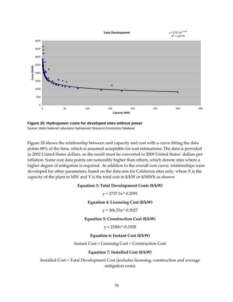
78
Total Development y = 2737.5x-0.2091
R2 = 0.8779
0
500
1000
1500
2000
2500
3000
3500
4000
0 50 100 150 200 250 300 350
Capacity (MW)
Cos
ts ($
/kW
)
Figure 20. Hydropower costs for developed sites without power Source: Idaho National Laboratory Hydropower Resource Economics Database
Figure 20 shows the relationship between unit capacity and cost with a curve fitting the data points 88% of the time, which is assumed acceptable for cost estimations. The data is provided in 2002 United States dollars, so the result must be converted to 2009 United States’ dollars per inflation. Some cost data points are noticeably higher than others, which denote sites where a higher degree of mitigation is required. In addition to the overall cost curve, relationships were developed for other parameters, based on the data sets for California sites only, where X is the capacity of the plant in MW and Y is the total cost in $/kW or $/MWh as shown:
Equation 3: Total Development Costs ($/kW)
y = 2737.5x^‐0.2091
Equation 4: Licensing Cost ($/kW)
y = 306.53x^‐0.3027
Equation 5: Construction Cost ($/kW)
y = 2180x^‐0.1928
Equation 6: Instant Cost ($/kW)
Instant Cost = Licensing Cost + Construction Cost
Equation 7: Installed Cost ($/kW)
Installed Cost = Total Development Cost (includes licensing, construction and average mitigation costs)

79
Equation 8: Fixed O&M Costs ($/kW)
y = 23.707x^‐0.2469
Equation 9: Variable O&M Costs ($/MWh)
y = 4.9659x^‐0.2024
The above equations were used to estimate costs based on installed capacity (x = capacity, y = cost) for each parameter.
• Overnight costs ($/kW):
ο Average: $1,882
ο High : $3,046
ο Low: $1,006
• Fixed O&M ($/kW‐yr):
ο Average: $17.57
ο High: $28.83
ο Low: $9.88
• Variable O&M ($/MWh):
ο Average: $3.48
ο High: $5.54
ο Low: $1.90
Capacity factors can vary dramatically. The INL Resource Database lists average hydroelectric capacity factors for California to be 54.87%. When evaluating actual capacity factors for hydroelectric power plants in California, capacity factors were found to be much different. The evaluation was performed as follows:
• Actual output (MWh) for 2007 and nameplate ratings (MW) were obtained for all hydroelectric facilities in California from the Energy Information Administration (EIA).
• All units with a capacity below 1.5 MW were removed.
• All pumped storage facilities were removed.
• Capacity factors were calculated for all remaining sites.
• Some of the data was found to be in error with capacity factors at or below zero or above 100%. So all facilities with capacity factors reported showing below 10% and above 90% were removed (approximately 10% of the sites).

80
• From this data set, it was considered unrealistic to choose the extreme high and low values. A more realistic approach for modeling was to remove the top and bottom 5%. This resulted in 178 facilities remaining, which were used to estimate capacity factor.
ο Average: 30.4% (weighted average of all sites on the listing)
ο High: 61.5%
ο Low: 12.5%
Expected Cost Trajectories Hydroelectric power is a very mature technology with a limited number of sites available for generation. Costs are not foreseen to decrease with increased generation projects and no learning effects were modeled. Cost trajectories were determined solely by projected inflation from 2009 to 2029.
3.4.3. Hydro – Capacity Upgrade for Developed Sites With Power Technical and Market Justification Developed waterways without power in California include 26 sites with a total nameplate potential of 1,744 MW.71 Potential upgrades range in nameplate capacity from 2 MW to 600 MW with the average being approximately 80 MW.
Primary Commercial Embodiment California’s nearly 400 hydro plants, with a total dependable capacity of about 14,000 MW, are mostly located in the eastern mountain ranges. California state also imports hydro‐generated electricity from the Pacific Northwest (source: California Energy Commission).
The number of hydroelectric plants in California is expected to increase by 2018. It is uncertain what the number of plants and total installed capacity will be.
Cost Drivers Since hydroelectric is a very mature, well established technology, there have been no industry changes since August 2007 that have materially affected costs. Also no trends are foreseen that would materially affect future costs.
The primary cost drivers for this technology are as follows:72
Initial Costs:
• Licensing
71 Conner, Alison M., Ben N. Rinehart, and James E. Francfort. U.S. Hydropower Resource Assessment for California. U.S. Department of Energy. Idaho National Laboratory. DOE/ID‐10430(CA), October 1998.
72 Hall, Douglas G., Richard T. Hunt, Kelly S. Reeves, and Greg R. Carroll. Estimation of Economic Parameters of U.S. Hydropower Resources. U.S. Department of Energy. Idaho National Laboratory. Bechtel BWXT Idaho LLC and INL Hydropower Resource Economics Database, June 2003.

81
• Construction
• Environmental mitigation
• Fish and wildlife mitigation
• Recreation mitigation
• Historical and archeological mitigation
• Water quality monitoring
• Fish passage
The various types of environmental mitigation are site specific (all are not required for each site).
Annual Costs:
• Fixed O&M
• Operation supervision and engineering
• Maintenance supervision and engineering
• Maintenance of structures
• Maintenance of reservoirs, dams, and waterways
• Maintenance of electric plant
• Maintenance of miscellaneous hydraulic plant
• Variable O&M
• Water for power
• Hydraulic expenses
• Electric expenses
• Miscellaneous hydraulic power expenses
• Rents
• FERC annual charge
Current Costs Costs were developed through the INL Hydropower Resource Economics Database. This database was developed from surveys of existing hydroelectric facilities. In developing this database, regression models were built relative to each cost driver and applied to potential sites throughout the United States. The costs were converted to 2009 United States’ dollars for this study.
A manipulation of the data was required to convert the costs to the units necessary for use in the COG model. Only data for potential sites in California were used. With the database in the required units, relationships were developed between unit rated capacity and costs.

82
Total Development Cost y = 1761.2x-0.1889
R2 = 0.8141
0
500
1,000
1,500
2,000
2,500
0 100 200 300 400 500 600 700
Capacity (MW)
Cos
t ($/
kW)
Figure 21. Hydropower costs for increasing capacity Source: Idaho National Laboratory Hydropower Resource Economics Database
Figure 21 shows the relationship between unit capacity and cost with the data points fitting the curve 81% of the time, which is assumed acceptable for cost estimations. The data is provided in 2002 United States’ dollars, so the result must be converted to 2009 United States’ dollars per inflation. Some cost data points are noticeably higher than others, which denote sites where a higher degree of mitigation is required. In addition to the overall cost curve, relationships were developed for other parameters, based on the data sets for California sites only, where X is the Capacity of the plant in MW and Y is the total cost in $/kW or $/MWh as shown:
Equation 10: Total Development Costs ($/kW)
y = 1761.2x^‐0.1889
Equation 11: Licensing Cost ($/kW)
y = 209.95x^‐0.3027
Equation 12: Construction Cost ($/kW)
y = 1351.6x^‐0.1928
Equation 13: Instant Cost ($/kW)
Instant Cost = Licensing Cost + Construction Cost
Equation 14: Installed Cost ($/kW)
Installed Cost = Total Development Cost (includes licensing, construction and average mitigation costs)

83
Equation 15: Fixed O&M Costs ($/kW)
y = 23.707x^‐0.2469
Equation 16: Variable O&M Costs ($/MWh)
y = 4.7411x^‐0.1998
The above equations were used to estimate costs based on installed capacity (x = capacity, y = cost) for each parameter.
• Overnight costs ($/kW):
ο Average: $932
ο High: $1,871
ο Low: $637
• Fixed O&M ($/kW‐yr):
ο Average: $12.59
ο High: $27.05
ο Low: $8.77
• Variable O&M ($/MWh):
ο Average: $2.39
ο High: $5.00
ο Low: $1.60
The capacity factor average, high, and low are assumed to be the same as for hydro – developed sites without power.
Expected Cost Trajectories Hydroelectric power is a very mature technology with a limited number of sites available for generation. Costs are not foreseen to decrease with increased generation projects and no learning effects were modeled. Cost trajectories were determined solely by projected inflation from 2009 to 2029.

84
3.5. Solar 3.5.1. Technology Overview There are three types of solar electric generating technologies considered for cost modeling: solar parabolic trough (without energy storage), solar parabolic trough (with energy storage), and solar photovoltaic (Single Axis).
Solar Parabolic Trough – General: This is also known as concentrating solar power (CSP) which uses mirrors to reflect and concentrate sunlight onto receivers that collect the solar energy and convert it to heat. This thermal energy can then be used to produce electricity via a steam turbine or heat engine driving a generator.
The predominant CSP systems in operation in the United States are linear concentrators using parabolic trough collectors. In such a system, the receiver tube is positioned along the focal line of each parabola‐shaped reflector. The tube is fixed to the mirror structure, and the heated fluid–either a heat‐transfer fluid or water/steam–flows through and out of the field of solar mirrors to where it is used to create steam (or, for the case of a water/steam receiver, it is sent directly to the turbine), shown in Figure 22.
Figure 22. Solar parabolic trough electric generating system Source: U.S. DOE, EERE
Solar Parabolic Trough – Energy Storage Technology Considerations: The use of thermal energy storage technology enables the wider use of solar renewable energy as dispatchable power and provides grid flexibility for peak demand times. Currently, there are three commercialized technologies available for storing thermal energy from solar parabolic and power tower plants73:
73 Konrad, Tom. “IN DEPTH: Hot Debate over Thermal Storage.” CSP Today, April 20, 2009.

85
• Steam – The least suitable method for thermal energy storage, as it lends itself to only short‐term buffer storage, and used primarily to address short‐term transient needs such as intermittent cloud cover.
• Mineral oil and synthetic heat transfer fluids – An approach currently used with existing technology solar parabolic trough systems, as the fluid does not solidify at night as molten salt systems can (at temperatures below 221 deg. C). Mineral oil systems are approximately three times more expensive to operate than molten salt systems, due to the oil cost, and so are chiefly used for shorter term duration storage of 30‐60 minutes.
• Molten salt – Typical molten salt systems use a mixture of sodium nitrate and potassium nitrate (60% sodium nitrate – 40% potassium nitrate) heated above the melting point of 221 deg. C. Molten salt systems are currently used in power tower designs, and are being examined for implementation in parabolic trough systems. The cost of molten salt storage for a parabolic trough system, which is estimated at $90‐160/kW, is roughly three times the cost of storage for a power tower system, due to the amount of molten salt needed, wider field arrays and transport distances for the trough system.
Figure 23. Simplified molten salt storage process diagram Source: Concentrating Solar Power – From Research to Implementation, European Commission, 2007
The research team chose a molten salt thermal storage system for the best commercial embodiment of this storage technology because of the engineering and technical aspects of the molten salt approach. The molten salt storage technology currently in operation in Spain’s AndaSol project was first successfully demonstrated in a test loop at the parabolic trough

86
system operating in Kramer Junction, California. The AndaSol project provides 50 MW of generation capacity, with a molten salt storage system of 7.5 hours duration.74
For purposes of analysis, a molten salt storage system comprising six hours duration of energy storage was modeled and costed into the thermal storage case.
Solar Photovoltaic (Single Axis): Photovoltaic (PV) systems include the PV modules themselves and the balance of systems (BOS). The BOS includes mounting structures, wiring, overcurrent protection, and inverters (the electronic device that converts DC to AC electricity). The mounting structures can include trackers that follow the sun’s path throughout the day. A single‐axis tracker simply tilts from east to west, following the sun’s path throughout the day. An example of a single‐axis PV system is the 14.2 MW facility at Nellis Air Force Base (Figure 24).
Figure 24. Nellis Air Force Base PV installation Source: SunPower Corporation
3.5.2. Solar – Parabolic Trough Technical and Market Justification The research team selected parabolic trough technology because it is commercially available. CSP installations are producing electricity with a capacity of 354 MW since 1990 (source: NREL). With AndaSol 1 ‐3 one parabolic trough system with 50 MW is commercially running in Spain, and two additional 50 MW plants are under construction. Storage technology (molten salt) for seven full load hours is included in the AndaSol project. Storage or combined operation
74 “Concentrating Solar Power – From Research to Implementation.” European Commission, 2007.

87
with gas leads to extended operation hours per day. Additional projects in Greece and Spain are being planned.
Primary Commercial Embodiment California has nine parabolic trough CSP facilities in operation. They are all in the Mojave Desert and were built between 1985 and 1991. One is rated at 13.8 MW, six at 30 MW, and two at 80 MW. The reason for these sizes is the 13.8 MW plant was the first one built as a demonstration, the 30 MW plants were sized per PURPA restrictions in place at the time, and the 80 MW plants were built when PURPA restrictions were raised to 80 MW plants in 1989. There are currently no such PURPA restrictions in place for plant size (source: EIA).
In these plants, solar trough technology is used to produce steam in a conventional steam turbine generator. Natural gas was used as a supplementary fuel for up to 25% of the heat input.
In 2018, the research team expects that the primary commercial embodiment will tend toward larger systems. The current primary worldwide commercial embodiment today is in Spain, where feed‐in tariffs have encouraged solar development, but system sizes are less than 50 MW due to restrictions in the feed‐in tariff system. Solar Millennium has announced a 250 MW parabolic trough power station in Nevada.75 An engineer at Solar Millennium told the research team that the system will consist of one 250 MW steam turbine (not 50 MW modules).
According to the engineer at Solar Millennium, the company believes 250 MW and expects to be the optimal size for parabolic trough systems and expects future systems to range from 200 to 300 MW. For smaller systems the turbine is too small (and therefore too expensive), and for bigger systems the losses in the solar collector field would be too high.
Cost Drivers Market and Industry Changes
Spain has one of the most favorable feed‐in tariffs for CSP plants paying at least United States’ $0.39 per kWh. That is one reason why at the end of 2007 more than 50 CSP projects with about 2,150 MW have been registered by Spain’s Ministry of Industry, making Spain the leading country in CSP development worldwide.
The first power station AndaSol 1 (50 MW) was commissioned in November 2008. AndaSol 2 (50 MW) is under construction, and AndaSol 3 (50 MW) will follow in 2009. All plants are equipped with six hours of molten salt storage. Due to the restrictions of the feed‐in tariff law in Spain the capacity of the units is limited to 50 MW at maximum.
75 Solar Millenium. Nevada Energy, Solar Millennium and MAN Ferrostaal Cooperate in the Development of Projects. Solar Millenium Corporate News, April 3, 2009. http://www.solarmillennium.de/Press/Press_Releases/Nevada_Energy__Solar_Millennium_and_MAN_Ferrostaal_cooperate_in_the_development_of_projects,lang2,50,1532.html.

88
Current Trends
For 2009, the Spanish government has announced a change in the feed‐in tariff. This will reduce the amount of new registered projects in Spain. Nevada Energy, Solar Millenium, and MAN Ferrostaal have announced a solar thermal power plant with a capacity of 250 MW and thermal storage capacity. Abengoa Solar has signed an agreement with Arizona Public Service (APS) to build and operate what will be the largest solar power plant in the world. The plant will be installed about 100 kilometers southwest of Phoenix, near Gila Bend. Solana, with 280 MWe of power output capacity, is based on parabolic trough technology and thermal storage using molten salts. It uses a single steam turbine.
Cost Drivers
The primary general cost drivers for parabolic trough systems are:
• Site work infrastructure.
• Solar field – Mirrors and solar receivers are the cost drivers of the system. Assumptions: Mass production of both elements could reduce costs.
• Steel price – Steel doubled in price between January 2008 and September 2008 and again between September 2008 and January 2009.
• Heat transfer fluid system.
• Thermal energy storage – Including thermal storage causes increases in cost due to the addition of the thermal energy storage system and additional solar field area required to charge the thermal storage system.
• Power block – Optimum size could reduce price of turbine and generator.
• Balance of systems.
• Contingency.
• Indirect costs.
Current Costs From the three basic studies the following actual cost data were extracted:

89
Table 18. Parabolic trough cost comparison
CEG-Study 2007 NREL-Study 2006 RETI 2008
Navigant Black & Veatch Black & Veatch $ € $ € $ €
Gross Plant Capacity (kW)
63,500
Net Plant Capacity (kW)
50,000 100,000 200,000
Annual Degradation (%/y)
0.2%
Project lifetime (y) 30 Overnight Cost ($/kW)
3,900 3,120 4,944 3,955 3,900 3,120
Site Work & Infrastructure
39 31 25 20
Solar Field 1,755 1,404 2,309 1,847 Heat Transfer Fluid System
78 62 100 80
Thermal Energy Storage (6 hrs.)
507 406 580 464
Power Block 312 250 388 310 Balance of Plant 195 156 225 180 Contingency 234 187 307 246 Indirect Costs 780 624 1,011 809 Fixed O&M ($/kW/y)
60 48 67 54 66 53
Variable O&M ($/MWh)
Development Time (months)
20 20 20
Construction time 12 12 12 Forced Outage Rate (%)
6% 6% 6%
Typical Net Capacity Factor (%)
27% 27% 27%
Source: CEG-Study: Klein and Rednam. Comparative Costs of California Central Station Electricity Generation Technologies. NREL-Study: Stoddard, Abrecunus, and O’Connell. Economic, Energy, and Environmental Benefits… RETI: Black & Veatch. Renewable Energy Transmission Initiative Phase 1A.
There are no actual published cost data available for the installations in Spain. In a publication downloaded from the homepage of Solar Millennium a number of 300 million euro (€) is mentioned. This would lead to specific costs of 7,500 $/kW.

90
From the same homepage a press release concerning the cooperation of Nevada Energy, Solar Millennium, and MAN Ferrostaal a CSP station with a capacity of 250 MW is announced with an investment volume of over 1 billion United States’ dollars. This would lead to investment costs of over 4,000 $/kW.76
Press releases concerning the 64 MW ACCIONA CSP project in the Nevada desert report investment costs between 220 million and 266 million United States’ dollars. This would lead to specific investment costs of 3,438 and 4,156 $/kW.77
Technology assumptions: 520,000 m² parabolic trough solar field (SKAL‐ET), cases include both non‐storage systems, a 6‐hour reserve molten‐salt thermal storage system, and a 250 MW‐capacity steam cycle. The technology case that includes six‐hour molten‐salt thermal storage also accounts for a 57% solar field area increase, used to charge the storage system and to improve capacity factor.78
Expected Cost Trajectories The direct costs of a parabolic solar plant can be summarized into the following five major categories:
• Siteworks and infrastructure
• Solar field
ο Heat Collection Element (HCE)
ο Mirror
ο Support structure
ο Drive
ο Piping
ο Civil work
• Power block
ο Steam turbine and generator
ο Electric auxiliaries
ο Thermal storage/heat transfer fluid system
ο Balance of Plant (BOP)
• Cooling system
• Water treatment
• Electrical
76 http://www.solarmillennium.de/index,lang2.html.
77 http://www.acciona‐energia.com/default.asp?x=0002020401&lang=En.
78 National Renewable Energy Laboratory, “Overview on use of a Molten Salt HTF in a Trough Solar Field,” NREL/PR‐550, February 2003.

91
• Instrumentation and control
• Miscellaneous civil work
The solar field, thermal storage, and power block costs encompass approximately 95% of the total direct costs, as illustrated in Figure 25. Of these three highest cost categories, the solar field cost comprises 58% of the total direct cost. Figure 25 shows the solar field component cost breakdown. The component cost breakdown of the solar field reveals the support structures are 29%, the heat collection elements 19%, and the mirrors 18% of the solar field direct costs, for a total of 68% of the solar field direct costs.
2%
58%23%
3%
14%
Structures and Improvements
Solar Collections System
Thermal Storage System
Steam Gen. or HX System
Power Block (EPGS, BOP)
Figure 25. Major cost categories for parabolic trough plant Source: NREL, Assessment of Parabolic Trough and Power Tower Solar Technology…
Table 19 provides a summary of SunLab’s design, deployment, and cost projections for trough plants with the SEGS VI plant as the base case.
Table 19. Assessment of parabolic trough and power tower solar technology
SEGS VI Trough 100 Trough 100 Trough 150 Trough 200 Trough 400
1999 2004 2007 2010 2015 2020 Plant size, net electric, MWe
30 100 100 150 200 400
Plant size, gross thermal input, MWt
88 294 279 408 544 1,087
Thermal Storage, hr
0 12 12 12 12 12
Annual Plant Capacity Factor
22.2% 53.5% 56.2% 56.2% 56.2% 56.5%
Annual Solar-to-Electric Efficiency
10.6% 14.2% 16.1% 17.0% 17.1% 17.2%
Solar Field Design:
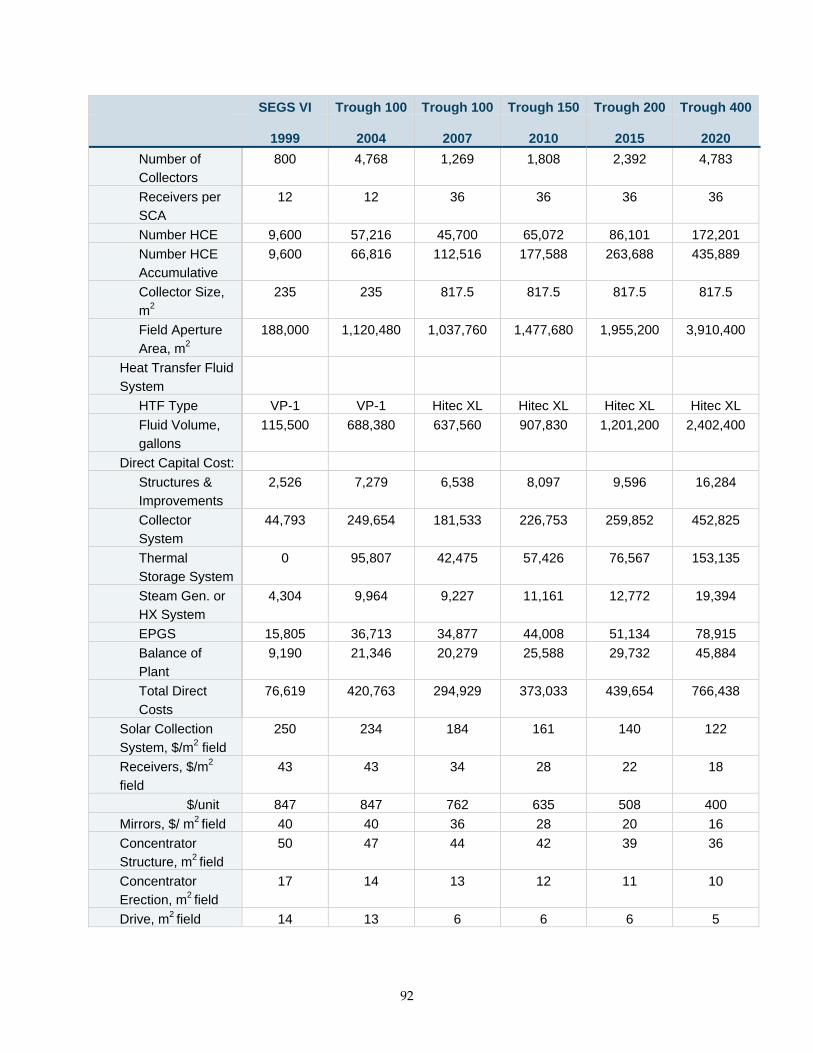
92
SEGS VI Trough 100 Trough 100 Trough 150 Trough 200 Trough 400
1999 2004 2007 2010 2015 2020 Number of Collectors
800 4,768 1,269 1,808 2,392 4,783
Receivers per SCA
12 12 36 36 36 36
Number HCE 9,600 57,216 45,700 65,072 86,101 172,201 Number HCE Accumulative
9,600 66,816 112,516 177,588 263,688 435,889
Collector Size, m2
235 235 817.5 817.5 817.5 817.5
Field Aperture Area, m2
188,000 1,120,480 1,037,760 1,477,680 1,955,200 3,910,400
Heat Transfer Fluid System
HTF Type VP-1 VP-1 Hitec XL Hitec XL Hitec XL Hitec XL Fluid Volume, gallons
115,500 688,380 637,560 907,830 1,201,200 2,402,400
Direct Capital Cost: Structures & Improvements
2,526 7,279 6,538 8,097 9,596 16,284
Collector System
44,793 249,654 181,533 226,753 259,852 452,825
Thermal Storage System
0 95,807 42,475 57,426 76,567 153,135
Steam Gen. or HX System
4,304 9,964 9,227 11,161 12,772 19,394
EPGS 15,805 36,713 34,877 44,008 51,134 78,915 Balance of Plant
9,190 21,346 20,279 25,588 29,732 45,884
Total Direct Costs
76,619 420,763 294,929 373,033 439,654 766,438
Solar Collection System, $/m2 field
250 234 184 161 140 122
Receivers, $/m2
field 43 43 34 28 22 18
$/unit 847 847 762 635 508 400 Mirrors, $/ m2 field 40 40 36 28 20 16 Concentrator Structure, m2 field
50 47 44 42 39 36
Concentrator Erection, m2 field
17 14 13 12 11 10
Drive, m2 field 14 13 6 6 6 5

93
SEGS VI Trough 100 Trough 100 Trough 150 Trough 200 Trough 400
1999 2004 2007 2010 2015 2020 Interconnection Piping, m2 field
11 10 3 3 3 2
Electronics & control, m2 field
16 14 4 4 4 3
Header piping, m2
field 8 7 7 6 6 5
Foundations/Other Civil, m2 field
21 18 17 15 14 12
Other (spares, HTF, freight), m2
field
17 17 11 10 9 8
Contingency, m2
field 12 11 9 8 7 6
Direct Capital Cost, $/kWe
Structures and Improvements, $/kWe
84 73 65 54 48 41
Solar Collection System, $/kWe
1,493 2,497 1,815 1,512 1,299 1,132
Thermal Storage System, $/kWe
0 958 425 383 383 383
System Generator of HX System, $/kWe
143 100 92 74 64 48
EPGS, $/kWe 527 367 349 293 256 197 Balance of Plant, $/kWe
306 213 203 171 149 115
Total Direct Cost, $/kWe
2,554 4,208 2,949 2,487 2,198 1,916
Source: NREL, Assessment of Parabolic Trough and Power Tower Solar Technology…
Table 20 and Figures 26 and 27 illustrate the SunLab projected total installed capital cost ($/kWe) compared to the more conservative (Sargent & Lundy) S&L values. Table 20 also shows the total installed capital cost based on achieving the annual net efficiencies projected by SunLab but not the projected cost reductions. The curves highlight the impact of the annual net efficiencies on the capital cost. The curves also indicate that additional cost reductions above the more conservative S&L values, due to technology improvements and increased deployment rates, will result in convergence of the capital costs toward the SunLab values.

94
Table 20. Comparison of total investment cost estimates ($/kWe): SunLab vs. S&L
2004 2007 2010 2015 2020
Sunlab $4,859 $3,408 $2,876 $2,546 $2,221 S&L – S&L Efficiencies $4,816 $3,854 $3,562 $3,389 $3,220 S&L - SunLab Efficiencies
$4,791 $3,687 $3,331 $3,165 $2,725
S&L – No Storage $2,453 $2,265 $2,115 $1,990 $1,846 Source: NREL, Assessment of Parabolic Trough and Power Tower Solar Technology…
Figure 26 Capital cost comparison Source: NREL, Assessment of Parabolic Trough and Power Tower Solar Technology…

95
Figure 27. Levelized O&M cost comparison Source: NREL, Assessment of Parabolic Trough and Power Tower Solar Technology…
Table 21. CSP plant capital cost breakdowns, 2005
($1,000s) 2007 100 MW*
2009 100 MW*
2011 150 MW*
2015 200 MW*
Site Work and Infrastructure
2,455 2,433 2,566 2,681
Solar Field 230,865 205,109 243,059 268,441 HTF System 10,009 9,895 11,896 13,542 Thermal Energy Storage 57,957 57,937 71,320 89,390 Power Block 38,754 38,754 48,899 56,818 Balance of Plant 22,533 22,533 28,432 33,036 Contingency 30,707 28,116 33,742 37,720 Total Direct Costs 393,280 364,776 439,915 501,627 Indirects 101,106 92,814 113,469 129,746 Total Installed Cost 494,386 457,590 553,384 631,373 *With 6 hours storage.
Source: Klein and Rednam, Comparative Costs of California Central Station Electricity Generation Technologies.

96
Table 22. Annual CSP O&M cost breakdowns, 2005
($1,000s) 2007 100 MW
2009 100 MW
2011 150 MW
2015 200 MW
Labor Administration 528 528 554 554 Operations 979 973 1,088 1,158 Maintenance 633 633 664 664 Total Labor 3,018 2,984 3,517 3,926 Miscellaneous 419 415 516 599 Service Contracts 263 259 352 435 Water Treatment 260 265 413 556 Spares and Equipment 669 651 870 1,040 Solar Field Parts and Materials
1,859 1,311 1,457 1,904
Annual Capital Equipment 226 218 320 418 Subtotal 3,695 3,119 3,928 4,953 Total 6,713 6,104 7,445 8,879 Source: Klein and Rednam, Comparative Costs of California Central Station Electricity Generation Technologies.
3.5.3. Solar – Photovoltaic (Single Axis) Technical and Market Justification Flat‐plate photovoltaic (FPV) modules are commercially available worldwide. The solar electricity market is booming. By the end of 2007, the cumulative installed capacity of solar PV systems around the world had reached more than 9,200 MW. This compares with a figure of 1,200 MW at the end of 2000. Installations of PV cells and modules around the world have been growing at an average annual rate of more than 35% since 1998 (source: EPIA).
On pvresources.com’s website almost 880 photovoltaic power plants (put into service in 2007 or earlier), each with peak power of 200 kWp or more, are listed. Cumulative power of all these photovoltaic power plants is about 955 MWp, and average plant power output is slightly more than 1.24 MWp. More than 390 large‐scale photovoltaic plants are located in Germany, 225 in the United States, and more than 130 in Spain (source: pvresources).
The PV modules can be mounted on fixed tilt strucures or on one or two axis tracking devices. As of December 2007, the market share of fixed arrays was 73% of the total installed capacity in large‐scale PV installations, only 27% were tracking systems (source: pvresources). However in situations with a high proportion of direct normal insolation, such as in California, the one‐axis tracking system could increase the sunlight capture by up to 25% over traditional fixed‐tilt systems, while significantly reducing land use requirements (source: Sunpower).

97
Primary Commercial Embodiment There are currently no single‐axis tracking utility‐scale PV installations in California. The largest FPV (single‐axis) project in the United States is 14 MWp at Nellis Air Force Base in Nevada.79 The actual construction and installation required eight months to complete (although it was in the planning stage for three years) and was complete in December 2007. The project is a public‐private partnership between the Air Force, Sunpower Corporation, Nevada Power Company, and MMA Renewable Ventures, a subsidiary of Municipal Mortgage and Equity.
The largest FPV (fixed tilt) project in the world is 60 MWp in Olmedilla, Castilla La Mancha, Spain.80 Germany also has a utility‐scale installation of FPV (fixed tilt) or 40 MWp in Waldpolenz, Brandis, Saxony, Germany.81
There is currently one utility‐scale single‐axis tracking PV systems planned for California and is planned to be in operation before 2018. PG&E has signed a contract with High Plains Ranch II, LLC, a subsidiary of SunPower Corporation, for 250 MW of high‐efficiency PV solar power. The plant would be located in San Luis Obispo Countyʹs California Valley. The project is expected to begin power delivery in 2010 and be fully operational in 2012.
Cost Drivers Market and Industry Changes
World solar PV market installations reached a record high of 5,750 MW in 2008, representing growth of 117% over the previous year.
Spainʹs PV market reached 2,600 MW in 2008 (annual growth rate of more than 400%) and now accounts for 44% of the world market. Germany reached a moderate increase to 1,500 MW, while the United States increased by 220% to 500 MW. It became the worldʹs third largest market even in front of Japan (once the world leader) which stayed stable at a level of 230 MW. (source: BSW‐Solar/EPIA/NNPVA)
Global solar cell production doubled in comparison to 2007 (3,436 MW). Chinese manufacturers raised their share in 2008. Meanwhile, thin film production reached a remarkable market share (2007: 12%).
In 2008, an interesting trend could be observed in Spain. Many large scaled PV installations have come into operation with capacities in the range of 20 to 60 MW (source: Photon).
Current Trends
In 2009 market experts and analysts expect the same rate of new installations as in 2008. The reasons for a reduction of the tremendous increase of the last two years are the financial crisis and the reductions of incentives especially in Spain and Germany.
79 www.sunpowercorp.com
80 www.nobesol.com
81 www.juwi.de

98
The dynamic extensions of the production facilities in all steps of the production chain result in an increasing offer of solar modules. As a result this could lead to reduced prices and a change from seller’s market to buyer’s market.
The suppliers of silicon basic material for solar cells have announced plans to increase their production capacity to 150,000 tons per year, equivalent to 15 GW of solar cells (source: Photon).
The downward move in retail prices of last month has accelerated in March 2009. It is now three months in a row where the number of decreases has outpaced increases, and the same outcome has been true for four out of the last six months.
The last time the European price index dropped back in January, the move was driven mainly by exchange rate movements within Europe. This time it is a function of actual price reductions, which were widespread across several retailers. This caused the European index to fall 7 cents per watt. The last time there was a drop of this magnitude was in November 2001.
While European prices reacted to market conditions, United States’ retailers also reduced prices. The movement in the United States index matched the drop seen in February.
These price drops are, in part, an outcome of the billions of dollars of investment made around the world in new manufacturing capacity for solar modules over recent years. As consumers demand this new energy source, so market size and production volumes allow the industry to bring down costs.
Cost Drivers
The primary general cost drivers for FPV single‐axis systems are:
• Solar modules – Cost of basic material silicon, wafers, and solar cells. Assumption: producers have increased their capabilities to produce silicon dramatically. Overcapacities are expected for the next three years.
• Inverters – Mass production of inverters cuts costs.
• Installation – Efficiencies of solar modules: High‐efficiency solar modules (mono‐crystalline) reduce cost of installation. Cheaper amorphous silicon modules increase cost.
• Steel price – Steel doubled in price between January 2008 and September 2008 and again between September 2008 and January 2009.
• Balance of systems.
• Marketing sales taxes.
• Gross margin.

99
Current Costs The Solarbuzz consultancy report analyzed the price of a single photovoltaic module by observing the prices of approximately 1.500 solar modules:
Figure 28. Solar module retail/price index, 125 watts and higher Source: http://www.solarbuzz.com/Moduleprices.htm
As of March 2009, there are currently 293 solar modules priced below $4.75 per watt (€3.75 per watt) or 20.1% of the total survey. This compares with 250 priced below $4.75 per watt in February. The lowest retail price for a multicrystalline silicon solar module is $3.29 per watt (€2.60 per watt) from a German retailer. The lowest retail price for a monocrystalline silicon module is $3.48 per watt (€2.75 per watt), also from a German retailer.
The lowest thin film module price is at $2.47 per watt (€1.95 per watt) from a Germany‐based retailer. As a general rule, it is typical to expect thin film modules to be at a price discount to crystalline silicon (for like module powers). This thin film price is represented by a 44 watt module.
The results of a yearly independent interview with 100 leading PV installation companies in Germany show that system prices for 100 kW roof‐mounted PV installation been reduced to a level of $4.96 per watt (€3.92 per watt) (without sales tax) in the first quarter of 2009.

100
Figure 29. Solar power generation plant since 2006 over 20% cheaper Source: http://www.solarwirtschaft.de/medienvertreter/infografiken.html
For a German installation of a PV power station (Waldpolenz/Rote Jahne) with a capacity of 30 MWp, total investment costs were reported at $4.49 per watt (€3.55 per watt).
For a second German installation of a PV power station (Königsbrück) with a capacity of 4.4 MWp, total investment costs were reported at $4.81 per watt (€3.80 per watt).
Both installations are fixed tilt.
Technology assumptions: The primary commercial embodiment of the technology for the cost model is 100,000 solar modules, multicrystaline silicon, area: app. 145,000 m², module efficiency: 14%, single‐axis tracking, 200 DC/AC inverters.
Expected Cost Trajectories The overall target of the short‐term research described in the Strategic Research Agenda (SRA) issued by the European Community is for PV electricity to be competitive with consumer electricity (grid parity) in southern Europe by 2015. Specifically, this means reaching PV generation costs of €0.15 per kWh ($0.19 per kWh), or a turnkey system price of €2.5 per watt ($3.16 per watt). This system price arises from typical manufacturing and installation costs of <€2.0 per watt ($2.5 per Watt). All cost and price figures are in constant 2007 values.

101
Figure 30. Typical turnkey system price Source: cordis.europa.eu/technology-platforms/pdf/photovoltaics.pdf
Based on a detailed analysis of cost reduction potentials, the working group of the SRA decided that the same cost targets shall be used for all flat‐plate PV module technologies considered: €0.8‐1.0 per watt ($1.01‐1.26 per watt) for technology ready by 2013 and implemented in large‐scale production in 2015, €0.60‐0.75 per watt ($0.76‐0.95 per watt) in 2020, and €0.3‐0.4 per watt ($0.38‐0.51 per watt) in 2030. The targets are expressed as a range to reflect the efficiencies of different types of modules. To meet the overall, cross‐technology cost targets, lower efficiency modules need to be cheaper than higher efficiency modules due to the area‐related component of the BOS costs. These targets should not be interpreted as predictions. It is possible that some technologies will even exceed them. The efficiency targets quoted later in the SRA for each technology are considered as performance targets that should be met to meet the cost target. System costs and prices, it should be noted, depend on the specific application that the system is put to. Therefore the costs and prices mentioned in the SRA are only approximate.

102
3.6. Wind 3.6.1. Technology Overview A wind energy system transforms the kinetic energy of the wind into electrical energy that can be harnessed for practical use. The main components of a wind turbine are as follows:
• A rotor, or blades, which convert the windʹs energy into rotational shaft energy.
• A nacelle (enclosure) containing a drive train, usually including a gearbox and a generator.
• A tower to support the rotor and drive train.
• Electronic equipment, such as controls, electrical cables, ground support equipment, and interconnection equipment.
Some wind turbines use direct‐drive generators and do not need a gearbox (being a critical component from a maintenance perspective).
Typical facilities today consist of 1.5 to 2.5 MW turbines atop 80 m towers.
Figure 31. A modern 1.5 MW wind turbine installed in a wind power plant Source: U.S. DOE, EERE, 20% Wind Energy by 2030. 82
82 U.S. Department of Energy. Energy Efficiency and Renewable Energy (EERE). 20% Wind Energy by 2030, Increasing Wind Energy’s Contribution to U.S. Electric Supply. DOE/GO‐102008‐2567, July 2008.

103
Wind plants can range in size from a few megawatts to hundreds of MW in capacity. Wind power plants are modular, which means they consist of small individual modules (the turbines) and can easily be made larger or smaller as needed. Turbines can be added as electricity demand grows. Today, a 50 MW wind farm can be completed in 18 months to two years. Most of that time is needed for measuring the wind and obtaining construction permits–the wind farm itself can be built in less than six months.
Some areas of California have good (Class 3/4) to excellent (Class 6/7) wind resources as seen in Figure 32.
Figure 32. California wind resource map Source: California Energy Commission PIER web site

104
California also has several wind power plants in operation. The specific locations of those plants are shown in Figures 33 and 34.
Figure 33. Wind resource map of Northern California Source: California Energy Commission. Wind Power Generation Trends at Multiple California Sites. PIER Interim Project Report, CEC-500-2005-185.

105
Figure 34. Wind resource map of Southern California Source: California Energy Commission. Wind Power Generation Trends at Multiple California Sites. PIER Interim Project Report, CEC-500-2005-185.
From Figures 33 and 34, wind classes were determined for the five California utility‐scale wind facilities. Also average capacity factors from 1995 to 2005 were determined.83
Altamont: Class 3‐4 18.4
San Gorgonio: Class 7 29.2
Tehachapi: Class 7 26.6
Pacheco: Class 2‐4 16.6
Solano: Class 4‐5 17.7
Capacity factor can vary from year to year. Also wind turbines are becoming more efficient, with greater capacity ratings and higher towers, thus producing higher capacity factors. Trends in capacity factor for these sites, from 1995 to 2005 are shown in Figure 35.
83 Electronic Wind Performance Reporting System (eWPRS), http://wprs.ucdavis.edu/

106
Figure 35. Capacity factor trends of California utility wind sites Source: eWPRS web site
These capacity factors include both older and newer installed turbines, so is not necessarily representative of capacity factors that can be expected from new installations.
3.6.2. Onshore Wind – Class 5 Technical and Market Justification According to the American Wind Energy Association (AWEA), in 2008, with over 8,500 MW installed, wind power provided 42% of all the new generating capacity added in the United States, up from less than 2% of new capacity added in 2004. With a total of 25,369 MW in operation at the end of 2008, the United States pulled ahead of the previous leader Germany (23,902 MW) both in wind energy production and in cumulative wind power generating capacity. The United States is also the world’s largest market in terms of new installations (8,545 MW) added in 2008, ahead of China (6,300 MW).
Primary Commercial Embodiment As of September 2008, California had 2517 MW of installed wind turbine capacity (source: AWEA). Wind plant installations are modular with the capability to add new turbines within

107
each development, thus increasing overall plant size. Recent wind turbine installations (since 2006) range in size from 1 MW to 3 MW (source: AWEA84).
Wind plant size in California varies dramatically. As an illustration, wind plant installations since 2003 are shown in Table 23. Plant sizes vary from less than 1 MW to 150 MW, and many of these installations are within the same general area as pre‐existing installations, which illustrate the modular nature of this technology. California installations listed by AWEA total 116 wind plants.
Utility‐scale wind turbine installations will continue to increase in California through 2018 and beyond. A growing trend is toward larger turbines. There are currently several 5 MW wind turbines in the prototype stage.85 It is uncertain whether such large turbines will be routinely installed for onshore applications or will be relegated only to the offshore market.
84 http://www.awea.org/projects/Projects.aspx?s=California
85 Musial, Walt, Sandy Butterfield, and Bonnie Ram. Energy from Offshore Wind. National Renewable Energy Laboratory, NREL/CP‐500‐39450, February 2006.

108
Table 23. California utility wind plant installations since 2003
Name LocationPower
Capacity (MW)
Units Turbine Size Turbine Mfr. Developer Owner Power Purchaser Year
Online
Shiloh II Northern California 150 75 2 REPower enXco enXco PG&E 2009
Edom Hills repower Southern California 20 8 2.5 Clipper BP Alternative Energy BP Alternative Energy SCE 2008
Alite Wind Farm Southern California 24 8 3 Vestas Allco/Oak Creek Energy California Portland Cement 2008
Dillon Southern California 45 45 1 Mitsubishi Iberdrola Renewables Iberdrola Renewables Southern California Edison 2008
Solano Wind Project Solano 63 21 3 Vestas Sacramento Municipal Utility District
Sacramento Municipal Utility District
Sacramento Municipal Utility District
2007
Buena Vista Altamont Pass 38 38 1 Mitsubishi Babcock & Brown Babcock & Brown Pacific Gas & Electric 2006
Shiloh Wind Power Project Solano County 150 100 1.5 GE Energy PPM Energy PPM Energy PG&E, Modesto Irrigation District & City of Palo Alto Utilities
2006
Solano IIA Solano County 24 8 3 Vestas Sacramento Municipal Utility District
Sacramento Municipal Utility District
Sacramento Municipal Utility District
2006
Coram Energy (Aeroman repower) Tehachapi 10.5 7 1.5 GE Energy Coram Energy Coram Energy Southern California Edison 2005
Kumeyaay Wind Power Project East of San Diego 50 25 2 Gamesa Superior Renewable Energy Babcock & Brown San Diego Gas & Electric 2005
Victorville Wind Project Victorville prison 0.75 1 0.75 Vestas NORESCO NORESCO Victorville Prison 2005
Victory Garden Tehachapi 0.66 1 0.66 Vestas Caithness Caithness Southern California Edison 2005
Victory Garden Tehachapi 6 8 0.75 Zond Caithness Caithness Southern California Edison 2005
Coram Energy (Aeroman repower) Tehachapi 4.5 3 1.5 GE Energy Coram Energy Coram Energy Southern California Edison 2004
Diablo winds Altamont Pass 20.46 31 0.66 Vestas FPL Energy FPL Energy Pacific Gas & Electric 2004
Lake Palmdale Palmdale 0.95 1 0.95 Vestas Palmdale Water District Palmdale Water District Palmdale Water District 2004
Oasis Power Partners Tehachapi 60 60 1 Mitsubishi enXco enXco San Diego Gas & Electric 2004
Solano Wind Project, phase II Solano County 4.62 7 0.66 Vestas FPL Energy Sacramento Municipal Utility District
Sacramento Municipal Utility District
2004
Aeroman repower (2003) Tehachapi 3 2 1.5 GE Energy Coram Energy Coram Energy Southern California Edison 2003
CalWind II CEC Tehachapi 8.58 13 0.66 Vestas CalWind Resources Southern California Edison 2003
High Winds Solano 162 90 1.8 Vestas FPL Energy FPL Energy PPM Energy 2003
Karen Avenue II (San Gorgonio Farms) San Gorgonio 4.5 3 1.5 GE Energy San Gorgonio Farms San Gorgonio Farms Southern California Edison 2003
Mountain View Power Partners III San Gorgonio 22.44 34 0.66 Vestas PPM Energy PPM Energy San Diego Gas & Electric 2003
Solano Wind Project, phase I Solano County 10.56 16 0.66 Vestas Sacramento Municipal Utility District
Sacramento Municipal Utility District
Sacramento Municipal Utility District
2003
Whitewater Hill San Gorgonio 4.5 3 1.5 GE Energy Cannon Power Corp. Cannon Power Corp. 2003 Source: AWEA Project Database

109
Cost Drivers Market and Industry Changes
There are several key market and industry changes since 2007 that have materially affected wind turbine installation costs.
• The value of the United States’ dollar relative to the Euro has shown an increase since mid‐2008.
• United States’ manufacturing of turbine parts has been increasing.
These changes and their significance are further discussed below.
Current Trends
The cost of wind power installations showed a steady decline from the early 1980s until 2002. Since then costs have increased steadily. This trend is from a Lawrence Berkeley National Laboratory (LBNL) study of actual installations over time and shown in Figure 36.86
Figure 36. Installed wind project costs over time Source: Wiser and Bollinger, Annual Report on U.S. Wind Power Installation, Cost, and Performance Trends: 2007.
These cost increases are driven by several market factors as discussed below (Wiser 2007):
• Increased cost for commodities (affecting turbine prices).
• Drop in value of the United States’ dollar relative to the euro.
• Improved sophistication of turbine design.
86 Wiser, Ryan and Mark Bolinger. Annual Report on U.S. Wind Power Installation, Cost, and Performance Trends: 2007. U.S. Department of Energy. EERE, May 2008.

110
• Upscaling of turbine size (and hub height).
• Shortages in certain turbine components.
• A general move by manufacturers to improve their profitability.
These factors are cited as reasons for wind turbine price increases of 9% from 2006 to 2007. But some of these factors have actually shown a reversal since 2007.
• The value of the United States’ dollar relative to the euro has shown an increase from mid‐2008 through April 2009 (Figure 38).
• United States’ manufacturing of turbine parts have increased from 30% in 2005 to 50% in 2008,87 thus reducing the value of the United States’ dollar relative to the euro as a cost driver.
• The increase in United States’ manufacturing capacity also results in a reduction on shortages of certain turbine components.
• There is speculation that direct drive88 or multiple generator drive train89 wind turbine configurations will ultimately reduce costs. Currently these technologies are in the development/demonstration stages.
Increased Cost for Commodities:
A wind turbine is made primarily of steel (approximately 90%) and other materials. Cost trends for these raw materials are shown in Figure 37.
87 Cheeseman, G.M. U.S Wind Turbine Manufacturing Will Increase. www.Clesias.com http://www.celsias.com/article/us‐wind‐turbine‐manufacturing‐will‐increase/
88 deVries, Eize. “REW Exclusive: Siemens New 3.6 MW Direct‐Drive ‘Concept’ Wind Turbine.” Renewable Energy World, July 4, 2008. http://www.renewableenergyworld.com/rea/news/article/2008/07/rew‐exclusive‐siemens‐new‐3‐6‐mw‐direct‐drive‐concept‐wind‐turbine‐52963
89 Cotrell, J.A. A Preliminary Evaluation of a Multiple‐Generator Drivetrain Configuration for Wind Turbines. Presented at American Society of Mechanical Engineers Wind Energy Symposium, NREL/CP‐500‐31178, January 2002. http://www.osti.gov/bridge/servlets/purl/15000704‐XNgzBn/native/15000704.PDF.

111
Figure 37. Metal prices Jan. 2002 – Sept. 2007 (London Metal Exchange) Source: O’Connell and Pletka, 20 Percent Wind Energy Penetration in the United States. 90
Drop in Value of the United States’ Dollar Relative to the Euro:
One factor in the cost increase for the wind industry since 2002 has been the drop in value of the dollar against the euro. Prior to 2008, the majority of wind turbine components have been manufactured in Europe, but this trend has started to reverse due to more United States’ manufacturing. As the value of the United States’ currency dropped against the euro, turbine prices have increased in United States’ dollar terms (Black & Veatch 2007). But this trend in value of the United States’ dollar against the euro has shown a reversal over the past year. This is illustrated in Figure 38.
90 O’Connell, Ric and Ryan Pletka, et al. 20 Percent Wind Energy Penetration in the United States: A Technical Analysis of the Energy Resource. Black & Veatch Project: 144864, October 2007.

112
Figure 38. U.S. dollar vs. euro, Jan. 1999 through April 2009 (European Central Bank) Source: European Central Bank.
Improved Sophistication of Turbine Design
Such improvements will include improved efficiencies resulting in increased capacity factors. Figure 39 shows capacity factor trends from wind turbine installations over time. This upward trend cannot be attributed only to turbine design. Increased hub heights and increased care in selecting turbine location for higher wind sites can increase capacity factor. The increase in hub height and care in site selection can also contribute to increased installed costs.
Figure 39. 2007 Project capacity factors by commercial operation date Source: Wiser and Bollinger, Annual Report on U.S. Wind Power Installation, Cost, and Performance Trends: 2007.
Projections of future capacity factor have been performed (Black & Veatch 2007) by analyzing monthly data from over 5,000 MW of wind plants installed in the Midwest from 2000 to 2005. The research team believes the Midwest installation analysis is transferable to California even though the topography is quite different, since capacity factors were determined by wind power class. One region, the Midwest, was chosen for the analysis with the purpose of performing a relative comparison. A regression curve was developed for the various wind classes and is shown in Figure 40.

113
Figure 40. Onshore capacity factor by installed year and class Source: O’Connell and Pletka, 20 Percent Wind Energy Penetration in the United States.
UpScaling of Turbine Size (and Hub Height):
Wind turbine size (ratings in MW), which drives rotor diameter and hub height, has increased over time. The increased equipment costs will be at least partially offset by increased capacity factor.
Table 24. Size distribution and number of turbines over time
Source: Wiser and Bollinger, Annual Report on U.S. Wind Power Installation, Cost, and Performance Trends: 2007.
Shortages in Certain Turbine Components
United States wind power capacity surged by 46% in 2007, with 5,329 MW added and $9 billion invested (Wiser 2007). Annual growth of the wind turbine industry in the United States is

114
shown in Figure 41, which has contributed to shortages in the industry. But as United States’ manufacturing capacity increases, turbine component shortages should be less of an issue.
Figure 41. Annual and cumulative growth in U.S. wind power capacity Source: Wiser and Bollinger, Annual Report on U.S. Wind Power Installation, Cost, and Performance Trends: 2007.
A General Move by Manufacturers to Improve Wind Profitability
Since 2003, wind power generation costs have been cost‐competitive with other forms of generation but have been generally increasing as wholesale power prices increase.
Figure 42. Average cumulative wind and wholesale power prices over time Source: Wiser and Bollinger, Annual Report on U.S. Wind Power Installation, Cost, and Performance Trends: 2007.
Since wind produced electricity is becoming more valuable with increased electric prices, increased development of the technology can occur (resulting in higher capacity factors, hub heights, and turbine efficiencies), and more effort can be put into locating the turbines in the best wind sites. Wind turbine manufacturers and wind site developers are then able to charge more for their products.

115
Cost Drivers
Each of the current trends listed above can also be considered cost drivers. Each of those trends primarily affects turbine prices, which are typically 75% of overall project installation costs (Black & Veatch 2007). General project cost drivers are listed below:
• Turbine cost
• Reliability
• Permitting and site selection
• Land acquisition
• Transmission costs
Also when using national average cost data, adjustments must be made for differences in California. A 9% increase from national cost data should be applied to wind turbine project installations in California (Black & Veatch 2007).
Some consider economies of scale to be a cost driver for lowering costs. Since wind power plants are a modular technology, very few economies of scale have been seen from larger installations (Wiser 2008), as shown in Figure 43.
Figure 43. Installed wind project costs as a function of project size: 2006-2007 projects Source: Wiser and Bollinger, Annual Report on U.S. Wind Power Installation, Cost, and Performance Trends: 2007.
Current Costs The current costs were determined through the following steps:
• Use installed costs from the 2008 DOE study91 ($2007).
91 Wiser, Ryan and Mark Bolinger. Annual Report on U.S. Wind Power Installation, Cost, and Performance Trends: 2007. U.S. Department of Energy. EERE, May 2008.

116
• Project costs to $2009 adjusting from $2007 per inflation (adjusted 6.75% per Moody’s price inflators from 2007 to 2009).
• Adjust national average costs to California values (multiplying by 1.09).
ο Average 2007 installed cost: $1,710/kW
ο Average 2009 installed cost: $1825/kW
ο California 2009 installed cost: $1,990/kW
Also, reported installed United States’ costs for 2007 ranges from $1,240/kW to $2,600/kW (Wiser 2008). Adjusting to $2009 for California, the high and low costs are as follows:
• High 2009 installed cost for California: $3,025/kW
• Low 2009 installed cost in California: $1,440/kW
Fixed O&M is estimated to have a national average cost of $11.50/kW (Black & Veatch $2006), based on review of recent projects. This is increased for California by 9%. Fixed O&M costs consist of property taxes, insurance, site maintenance, legal fees, labor, and miscellaneous items.
It is assumed these factors can vary by approximately ±25% to obtain the high and low fixed O&M costs. The 25% value was determined through inspection of O&M variability (Wiser 2008).
Adjusting to $2009, fixed O&M cost: $13.70/kW:
Average: $13.70/kW
High: $17.13/kW
Low: $10.28/kW
Variable O&M costs are estimated to have a national average cost of $7.00/MWh (Black & Veatch $2006), based on review of recent projects. Variable O&M is driven by number of turbines and will decline as turbine reliability improves. Since the trend is toward larger wind turbines, resulting in fewer turbines per site, and higher quality products, variable O&M is expected to decline over time. Based on these factors, Black & Veatch estimates current variable O&M costs at $7.00/MWh and 2030 costs at $4.40/MWh, with an average of $5.00/MWh (all in $2006).
Adjusting to $2009, variable O&M cost:
Average: $5.50/MWh
High: $7.66/MWh
Low: $4.82/MWh

117
Expected Cost Trajectories Recent cost trajectories show a steep increase in wind turbine installed costs over the past several years. This report explains the various causes behind the increase. It is unreasonable to believe the costs will continue to climb. Many of the factors that have contributed to cost increases since 2002 have shown a reversal over the past two years. These factors include:
• Value of United States’ dollar versus the euro declined from 2002 to mid‐2008, but has shown a reversal since then.
• Increases in global and United States‐based manufacturing capacity for wind turbines.
• Basic commodity prices (e.g., steel, copper) have steadied and in some cases declined.
The research team has concluded a learning effect in wind turbine installations will be realized, but it is expected to be modest. The main driver being that wind generation in conjunction with the production tax credit (PTC) and investment tax credit (ITC) is currently cost competitive with other forms of generation. The learning effect is estimated between 0.33% to 0.5% per year.
3.6.3. Onshore Wind – Class 3/4 The entire discussion on Class 5 wind directly applies to Class 3/4 wind. The only difference is in the capacity factor, which can be determined from Figure 40. Capacity factor ranges for Class 3/4 wind turbine installations are given below:
Average: 37%
High: 41%
Low: 34%
3.6.4. Offshore Wind – Class 5 Technical and Market Justification Offshore wind is an emerging technology in the United States and an operational one in Europe. There are no installations in the United States, but by the end of 2008 a total of over 1,400 MW of offshore wind farms have been in operation around Europe; in the coastal waters of Denmark, Ireland, Netherlands, Sweden, the United Kingdom, Germany, Belgium, and Finland. This represents around 2% of the cumulative installed capacity of wind power in the European Union (EU) (source: EWEA). A breakdown of offshore wind installations by country is provided in Figure 44.

118
Figure 44. European offshore wind installations Source: EWEA, Seas of Change: Offshore Wind Energy.
Several offshore wind power installations have been proposed in the United States, but many have been postponed or cancelled purportedly due to high project costs.92 Other issues fostering opposition have been the perceived impact to scenery from valuable coastal properties, bird migration patterns, and hazards to marine and air navigation.93 Offshore wind has been seeing a slow start in the United States but should one day become a reality in many parts of the country. Off the Delaware shore, the first offshore wind farm to be developed in the United States has already sold one‐third of the power that will be generated during its first 25 ***years of operation before a turbine is even placed in the water.94
92 O’Connell, Ric and Ryan Pletka, et al. 20 Percent Wind Energy Penetration in the United States: A Technical Analysis of the Energy Resource. Black & Veatch Project: 144864, October 2007. 5‐10.
93 Snyder, John “Despite Opposition, Offshore Wind Farms Seem Poised to Make Their Mark.” Professional Mariner Magazine, September 2007.
94 Environmental News Service. “First U.S. Sale of Offshore Wind Power Signed.” January 2008.

119
Primary Commercial Embodiment There are currently no offshore wind installations in California.
The primary focus of offshore wind farms in the United States has been off the Atlantic coast. Strong wind resources also exist off the Pacific coast, but these are primarily in deep waters, which present technical challenges.95 Until these challenges associated with deep water wind platforms are resolved, offshore wind development in California will be limited.
Cost Drivers Market and Industry Changes
Market and industry changes have been presented in the Onshore Wind section, which also apply to offshore wind. There are additional changes that apply to offshore.
Due to Delaware’s mandate to guarantee stable prices for electricity (House Bill 6) and its RPS requirements of 20% renewable energy by 2019 (Senate Bill 74), Bluewater Wind negotiated a Power Purchase Agreement (PPA) with Delmarva Power for power from offshore wind. Bluewater is proposing a 450 MW plant.96
New United States’ policy framework, including commitments from the Department of the Interior, the Minerals Management Service, and the FERC encourage the development of offshore wind energy generation capacity.97
Another 30 state legislators have signed onto a letter to Kenneth L. Salazar, U.S. Secretary of the Interior, to quickly approve the Cape Cod Wind Farm project off the Massachusetts coast.98
In Europe, the offshore wind industry is flourishing. The EWEA’s statistics show that a total of 1,471 MW was installed worldwide by the end of 2008, all of it in European Union (EU) waters.
Since December 2007, the number of countries that host offshore wind turbines has increased from five to nine–that is, one third of EU Member States.
In 2008, Europe installed 357 MW, equivalent to almost 1 MW of offshore capacity being added every day (source: EWEA).99
95 U.S. Department of the Interior. Survey of Available Data on OCS Resources and Identification of Data Gaps. OCS Report. MMS 2009‐015, 2009.
96 http://www.bluewaterwind.com/de_overview.htm.
97 Jesmer, Graham, “Stage Set for Offshore Wind Energy in the U.S.” Renewable Energy World, April 8, 2009.
98 http://www.capewind.org/news973.htm.
99 EWEA. Seas of Change: Offshore Wind Energy, February 2009, http://www.ewec2009.info/fileadmin/ewec2009_files/documents/Media_room/EWEA_FS_Offshore_FINAL_lr.PDF.

120
Current Trends
Onshore wind energy trends also affect the offshore industry. Some trends particular to the offshore industry are noted:
• Onshore wind turbine sizes have shown a steady increase over the past several years (see discussion in Onshore Wind section). This is significant since the trend for offshore wind has been for larger size turbines.
• The EU potential for offshore wind development is foreseen to be 20 to 40 GW through 2020. Back in 2003, EWEA published projections of 70 GW of offshore wind by 2020. This projection was foreseen as unrealistic and was revised in 2007 to 20 GW to 40 GW.100
• Due to the EU target of 20% renewables by 2020, offshore wind is foreseen to play a significant factor. Trends of past installations with projections for future growth are provided by EWEA and shown in Figure 45.
Figure 45. European offshore wind growth and projections Source: EWEA, Seas of Change: Offshore Wind Energy.
100 EWEA. Delivering Offshore Wind Power in Europe. December 2007.

121
With increased international growth of the offshore wind industry, some installations off the California coast should be realized within the next 20 years.
Cost Drivers
Primary cost drivers for offshore wind installations are as follows:
• Turbine cost.
• Reliability and maintenance.
• Permitting and site selection.
• Support structure.
• Grid connection and transmission costs.
• Development of technology of foundations or floatation.
These cost drivers are very similar to those for onshore wind. One key difference is for onshore, the turbine is approximately 75% of project costs, where for offshore the turbine is approximately 33% of project costs.
Current Costs Both overnight and O&M costs of offshore wind installations have been estimated to be approximately twice that of onshore installations101 (also from Black & Veatch, page 5‐10).
Both the 2009 and 2018 Onshore Class 5 dollars have been doubled to obtain the necessary offshore wind project costs. For modeling purposes, it is estimated wind turbine installations will begin off the California coast in 2018.
Overnight Costs ($/kW):
$2009 $2018
Average: $3,980 $4,581
High: $6,050 $6,964
Low: $2,880 $3,315
101 Beurskens, L.W.M., M. de Noord, and H.J. de Vries. Potentials and Costs for Renewable Electricity Generation. Energy Research Centre of the Netherlands. ECN‐C–03‐006, February 2004.

122
Fixed O&M Costs ($/kW‐yr):
$2009 $2018
Average: $27.40 $31.54
High: $34.25 $39.42
Low: $20.55 $23.65
Variable O&M ($/MWh):
$2009 $2018
Average: $11.00 $12.66
High: $15.32 $17.63
Low: $9.64 $11.10
One other thing to note is the capacity factor. Due to larger wind turbines for offshore applications (meaning higher towers) and lower wind turbulence, capacity factors will increase by 15% over onshore turbine estimates (Black & Veatch 2007). Capacity factor estimations are included in Figure 46.
Figure 46. Offshore capacity factor by installed year Source: O’Connell and Pletka, 20 Percent Wind Energy Penetration in the United States.

123
Capacity factors for Class 5 offshore wind are estimated to vary between 42% and 48% with the average being 45%.
Expected Cost Trajectories Primary cost trajectories are to include learning effects as more offshore wind projects are installed. Period 1 & 2 Learning Rates (20% and 10% respectively), defined in EIA’s Electricity Market Module, were used to estimate cost reductions over time. It is estimated each learning rate will last five years. Therefore a total of 15% cost improvement will be realized between 2018 and 2029, based on increases in cumulative installed generation from 23 GW to 110 GW. This is a conservative estimate since onshore wind installations decreased in cost by 50% from 1982 to 1992.
3.7. Wave 3.7.1. Technology Overview Wave energy extraction is complex, and many device designs have been proposed. For understanding the device technology, it is helpful introduce these in terms of their physical arrangements and energy conversion mechanisms.
• Distance from shore – Wave energy devices may convert wave power at the shoreline, near to the shore (defined as shallow water where the depth is less than one half of the wavelength) or offshore.
• Bottom mounted or floating – Wave energy devices may be either bottom‐mounted or floating.
Wave energy devices can be classified by means of the type of displacement and reaction system employed. Various hydraulic or pneumatic power take off systems are used and in some cases the mechanical motion of the displacer is converted directly to electrical power (direct‐drive) Four of the most well‐known device concepts are introduced below and their principle of operation illustrated.
• Symmetrical point absorber – A bottom‐mounted or floating structure that absorbs energy. The power take‐off system may take a number of forms, depending on the configuration of displacers/reactors. The key characteristic of a point absorber is that it can absorb more energy than available within the devices width if the device is tuned (i.e., it is natural resonance frequency matches the incident wave frequency).
• Oscillating Water Column (OWC) –Nearshore or offshore, this is a partially submerged chamber with air trapped above a column of water. As waves enter and exit the chamber, the water column moves up and down and acts like a piston on the air, pushing it back and forth. The air is forced through a turbine/generator to produce electricity.
• Overtopping terminator – A floating reservoir structure with a ramp over which the waves topple and hydro turbines/generators through which the water returns to the sea.

124
• Attenuator – One form of the attenuator principle is a long floating structure that is orientated parallel to the direction of the waves. The structure is composed of multiple sections that rotate in pitch and yaw relative to each other. That motion is then converted to electricity using an electro‐hydraulic power conversion machine.
Conceptual diagrams of these devices an included in the following figures (source: EPRI).
Figure 47. Point absorber Source: EPRI, Ocean Tidal and Wave Energy…
Figure 48. Oscillating water column Source: EPRI, Ocean Tidal and Wave Energy…
Figure 49. Overtopping Source: EPRI, Ocean Tidal and Wave Energy…

125
Figure 50. Attenuator Source: EPRI, Ocean Tidal and Wave Energy…
3.7.2. Ocean Wave Technical and Market Justification Wave energy has been in existence for many years, although very few commercial developments are in place. Currently, worldwide installations total only 4 MW rated nameplate. There has recently been substantial interest, with over 25 countries involved in developing relevant conversion technologies for harnessing ocean renewable resources for electricity generation and/or other purposes. Also over the past two years there have been several companies submitting filings with the FERC for permits to install ocean wave energy systems in various locations along the California coast. These permits are for systems ranging in size from 1 to 5 MW to 100 MW.
Primary Commercial Embodiment There are currently no commercial wave energy systems installed off the California coast.
Based on the recent FERC filings, it is hypothesized that by 2018 there will be some commercial wave energy systems installed off the West Coast of the United States. The FERC filings have been for systems from up to 5 MW to up to 100 MW. In reality, each of these companies that have submitted filings and will perform some installations will perform more detailed evaluations of the site, begin installing ocean wave units, evaluate their performance, and then add more units to the plants based on their evaluations of performance and projected costs/benefits. A 40 MW typical plant size is foreseen as average based on the range of FERC filings.
Cost Drivers Market and Industry Changes
There have been no market and industry changes since August 2007 that have materially affected the costs of wave energy systems.

126
Current Trends
Based on a review of several FERC filings, it is foreseen that a few wave energy manufacturers will install demonstration projects to prove out their system and then add to the capacity based on their success. The filings show modularity with the systems, which allow adding onto capacity with multiple units.
Cost Drivers
Primary cost drivers for this technology are as follows:102
• Device structure – Required to house the wave energy turbine and generator.
• Mechanical and electrical plant – Shore‐based power station for the unit.
• Transportation and installation – Moving equipment to the shore and shipping to the off‐shore device structure.
• Construction management and permitting – Administrative costs.
• Electrical transmission – Undersea cables.
• Variable O&M – Cost of spares and repair costs (replacement parts and removal, replacement and refurbishment of parts).
• Fixed O&M – Operational costs (maintenance crews and vessels to enable repairs).
Current Costs The best cost information was found from a report published by the Energy Technology Support Unit (ETSU) of the Association for Educational Assessment (AEA) Europe.102 The report outlines the result of a European cost model developed in the early 1990s and refined in the late 1990s. It gives cost data and capacity factors for several competing wave energy technologies in 1999 British pounds.
British pounds (1999) were converted to 1999 United States’ dollars through historical exchange rates.
Equation 17: 1999 British pound to 1999 U.S. dollar Conversion
1999 U.S. dollar = 1.61 x 1999 British pound
United States’ dollars (1999) were converted to present and future dollars strictly through inflation estimates. A summary of the costs obtained and the costs calculated are included in Table 25.
102 Thorpe, Tom. A Brief Review of Wave Energy. AEA Technology. ETSU‐R120, May 1999.

127
Table 25. Ocean wave energy cost data
Device Rated Capacity
Capacity Factor
Estimated Cost (£)
Estimated Cost per
Unit (£/kW)
Estimated Cost per
Unit ($/kW)
Fixed O&M per
Unit (£/kW)
Fixed O&M per
Unit ($/kW)
Variable O&M per
Unit (£/MWh)
Variable O&M per
Unit ($/MWh)
Limpet 1 MW 0.206 £1,160,000 £1,160 $1,868 £13 $21 £4 $7Limpet II 1 MW 0.26 £1,400,000 £1,400 $2,254 £17 $27 £6 $9Ospray 20 MW 0.26 £26,300,000 £1,315 $2,117 £19 $31 £7 $11Duck 2 GW 0.3 £2,400,000,000 £1,200 $1,932 £21 $34 £7 $11
1999 cost $2,043 $28 $92018 cost $2,978 $41 $142009 cost $2,587 $36 $121999 cost $1,868 $21 $72018 cost $2,723 $31 $102009 cost $2,365 $27 $91999 cost $2,254 $34 $112018 cost $3,286 $50 $172009 cost $2,855 $43 $14
Averages 0.26
Low
High
0.21
0.30
Source: Thorpe, T.W.
Expected Cost Trajectories Learning effects from ocean wave technology are expected be modest since cumulative generation is not expected to be at a high enough level to take advantage of economies of scale.
3.8. Integrated Gasification Combined-Cycle 3.8.1. Technology Overview There are several major IGCC process technologies available for power generation. The main suppliers of gasifier technology are Shell, GE, Siemens, and ConocoPhillips. The research team did not focus on one of these process technologies to avoid excluding possible viable options for the future. Therefore the selected IGCC technology for this study is based on the current worldwide practice for coal‐fueled IGCC technology at a scale of 300 MW. This results in the selection of the oxygen‐blown entrained flow gasifier process technology.
Air‐blown gasification technology is available, but since it has not been applied outside of Japan, it is not considered as a primary commercial embodiment of the IGCC technology. This process does not require an air separation unit; however, the syngas contains a lot of nitrogen resulting in much larger dimensions of equipment than oxygen‐blown gasification.
Figure 51 shows a typical oxygen‐blown IGCC process schematic, and Figure 52 shows an aerial photo of an actual installation.

128
Figure 51. Typical oxygen blown IGCC process Source: KEMA
Steam/Feedwater
Condensate
Tailgas Waste water
Raw Cleaned Humidified HeatedSyngas Syngas Syngas Syngas
OxygenNitrogen Heated Nitrogen
DilutedSyngas
Cooled Compressed air GTcompressed air exh
ASU
Flyash
Slag Gas cleanup
Sulpur
Humidification
Waste water treatment unit
Gasificationisland
Steam cy
Suppletion water
Treated water
Residue
Ambient air
Ambient air
Stack gas
Gas turbine
Coal

129
Figure 52. Actual installation (Buggenum, The Netherlands) with typical technological components indicated Source: Google Earth, modified by KEMA
The basic principle of IGCC is the gasification (partial oxidation) of pulverized coal with oxygen and steam to produce a syngas, which is combusted in a gas turbine. The oxygen is supplied by an air separation unit which separates ambient air into oxygen and nitrogen. The air can be delivered by the compressor of the gas turbine (full air‐side integration) or by a separate compressor (no air‐side integration). Air‐side integration will lead to higher plant efficiency but also to more complex power plant operations. Current state‐of‐the‐art is partial air‐side integration.
Combined cycle (Steam+Gas)
Humidification
Air Separation Unit (ASU)
Gasification island
Waste water treatment unit
Gas cleanup

130
In the gasification island, coal (either supplied in slurry or in powder form) is gasified in the reactor into raw gas. Apart from the raw gas also fly ash and slag are formed. The raw gas contains:
• Combustible components CO and H2.
• Incombustible harmless components H2O, N2, Ar.
• Greenhouse gas CO2.
• Traces of environmentally and/or technically harmful gaseous components:
ο Sulphur: H2S and COS.
ο Halogens: HCl and HF.
ο Nitrogen: NH3, HCN.
ο Traces of alkali and heavy metals (such as mercury).
The raw gas is purified in the gas cleanup, that is removal of fly ash (via cyclone, filter, and/or wet scrubbing), heavy metals, halogen, nitrous compounds, alkali (wet scrubbing), and sulphur (absorption). During this process waste water and some tail gas are produced. The tail gas is recycled back into the gasification island while the waste water is cleaned in the waste water treatment plant. During this process clean distillate and residue are produced. The distillate is reused in the power plant.
The cleaned syngas is moisturized and diluted with nitrogen to achieve a lower heating value. This contributes to lower NOx‐emissions. Also the heat rate is improved marginally. To improve the heat rate further the humid syngas is heated by feedwater from the steam circuit between gasification island and steam cycle.
The diluted syngas is combusted under pressure in the gas turbine using ambient air pressurized by the gas turbine’s compressor. The hot combustion gases drive the gas turbine’s expander, providing electric power to drive compressor and generator. The exhaust gases are lead into the steam cycle where steam is produced in the waste heat boiler and is expanded in the steam turbine installation, producing electricity.
3.8.2. IGCC Without Carbon Capture (Single or Multiple 300 MW Trains) Technical and Market Justification Coal‐IGCC is a very promising new clean‐coal technology, especially because it is well‐ suited for CO2 capture. As illustrated by an increasing trend in announcements of new United States’ gasification projects, the United States’ market is aware of this potential applicability of coal‐IGCC for future power generation. The entities that are considering implementing IGCC projects include some major energy industry players such as AEP and Duke Energy (formerly Cinergy). In addition, numerous smaller companies are pursuing gasification projects using state and federal grants. The more advanced, publicly discussed IGCC projects are shown in Table 26. In total, based on information from public announcements, 50 projects have been identified for United States operation beyond 2010.

131
Table 26. Gasification-based power plant projects under consideration in the United States beyond 2010
Project Name/Lead Location Feedstock CT Fuel Net (MWe)
Orlando Gasification Project*/Southern Co., OUC Orlando, FL coal syngas 285
Lima Energy IGCC/Global Energy Lima, O coal/ petcoke syngas 540 SNG H2
Cash Creek IGCC Plant/GE, MDL Holdings Henderson County, KY coal syngas 630
Lockwood IGCC Plant/Hunton Energy, Cogentrix Energy Inc. Sugar Land, TX petcoke syngas 1200
Mesaba/Excelsior Energy Holman, MN coal/ petcoke syngas 600
Carson H2 Power Project/BP, Edison Mission Group Carson, CA petcoke H2 500
FutureGen/FutureGen Alliance Illinois or Texas coal H2 275
Mountaineer Plant/AEP New Haven, WV coal syngas 630
Pacific Mountain Energy Center/Energy Northwest Port Kalama, WA coal/ petcoke syngas 680
Taylorville Energy Center IGCC/CCG LLC Taylorville, IL coal syngas 630
Huntley IGCC Project/NRG Energy Tonawanda, NY coal syngas 680
Tampa Electric, Unit 2 Polk County, FL coal syngas 630
Wallula Energy Resource Center/Wallula Resource Recovery LLC Wallula, WA coal syngas 600-700
Xcel Energy Colorado coal syngas 300-350
TXU Corp. Colorado City, TX coal syngas 630
TXU Corp. Henderson, TX coal syngas 630
Clean Hydrogen Power Generation Project/Southern California Edison California coal H2 600
Indian River IGCC Project/NRG Energy Millsboro, DE coal syngas 630
Edwardsport IGCC Project/Duke Energy Edwardsport, IN coal syngas 630
Great Bend/AEP Meigs County, OH coal syngas 630
IGCC Demonstration Plant/Wyoming Infrastructure Authority, Pacific Corp Wyoming coal syngas TBD
Lower Columbia Clean Energy Center/ Summit Power Group Clatskanie, OR petcoke/ coal syngas 520
Mississippi Power Kemper County,
MS coal syngas 600
NRG Energy Texas coal syngas 630
Steelhead Energy/Madison Power Williamson County,
IL coal syngas 620 SNG Source: U.S. DOE, NETL, Gasification World Database 2007.
Primary Commercial Embodiment Currently, no new gasification plants are projected to come on‐line in the North American region from 2008 to 2010. This continues the trend from 2005 to 2007 where no new plants were started in the United States and only one plant, the Long Lake Plant, began operations in

132
Alberta, Canada. This absence of new United States capacity additions from 2005 to 2010 is understandable given that these plants would have had to be committed to during the late 1990s and early 2000s. In those years the natural gas prices were low, resources for industrial needs and transportation fuels were seemingly abundant, and the results from demonstrations of new generation gasification technologies (e.g., the Polk and Wabash IGCC plants) were not yet fully known. However, with expanded demand for power plants, concerns over the availability and prices of oil and gas, and increased consensus regarding the needs for deployment of technologies providing for environmental protection, gasification‐based projects are increasingly viewed as a technology option for future progress.103
The commercial applicability of coal‐fueled IGCC is demonstrated by approximately 18 IGCC projects throughout the world. One of these projects was the coal/petcoke‐based Cool Water IGCC plant, which has been decommissioned. Of the six currently operating coal IGCC plants, four are commercial‐scale, entrained flow gasification demonstration projects (ranging in capacity from 250 to 300 MW) and are located in Florida, Indiana, The Netherlands, and Spain.104 This information shows that entrained flow gasification technology has been selected by all six companies. As feedstock, bituminous coal is the main choice, followed by a blend of petcoke. The Southern Company/OUC project is based upon 100% Power River Basin coal but is a commercial demonstration project for a new gasification technology and the demonstration will not be complete until 2015. NRG Energy reports using a fuel supply of primarily coal but could include up to 20% petcoke and 5% biomass.
Current trends suggest that the IGCC of the future will contain much of what is seen now, with entrained gasification retaining its position as the most common system. The gas turbines will be based on the natural gas‐fired versions that will have been deployed a few years earlier. Hydrogen technology will probably be the safe option at that time. The larger capacity of the H‐class gas turbines will provide an economy of scale, helping to reduce the specific capital cost of IGCC. If, additionally, gasifier unit sizes have been successfully increased, and it becomes possible for a one‐on‐one gasifier/gas turbine combination to be used, this will provide further cost savings due to scale. Steam conditions in the steam cycle could then be raised to ultra‐supercritical, which will give further (modest) efficiency benefit.
Although the Coolwater IGCC demonstration plant built in California in the 1980s was the world’s first commercial‐scale IGCC demonstration plant, only one gasification project is currently under consideration in the state, a Clean Hydrogen project as shown in Table 26.
103 U.S. Department of Energy. Office of Fossil Energy. National Energy Technology Laboratory. Gasification World Database 2007, October 2007. <http://www.netl.doe.gov/technologies/coalpower/gasification/database/database.html>.
104 Black & Veatch. Clean Coal Technology Selection Study Final Report January 2007. Black & Veatch, 2007.

133
Cost Drivers Market and Industry Changes
Construction costs for power plants have escalated at an extraordinary rate since the beginning of this decade. Most recent change is the current credit crunch that will affect the demand and supply equilibrium in market. The effects on the cost price development for coal‐fueled IGCC power plants were analyzed.
Current Trends
The research team included the following trends in the cost analysis:
• Construction material costs.
• Equipment costs.
• Labor costs.
• Learning effects.
Data from the U.S. Bureau of Reclamation were used to assess trends in construction costs. These general construction cost trends were developed to track construction relevant to power generation project costs. This data was also compared with the Gasification World Database 2007 report, which shows that cost of original equipment and installation has increased as much as 20% to 30% since 1998.105 Figure 53 shows power plant construction costs and main components. The various cost indexes in the figure all consist of two elements: contractor labor and equipment costs and contractor supplied materials and equipment. A dramatic increase in costs is evident at the end of 2008, corresponding to the beginning of the credit crunch.
105 U.S. Department of Energy. Office of Fossil Energy. National Energy Technology Laboratory. Gasification World Database 2007, October 2007. <http://www.netl.doe.gov/technologies/coalpower/gasification/database/database.html>.

134
Bureau of Reclamation Construction Cost Trends
200
220
240
260
280
300
320
340
jan-00
jan-01
jan-02
jan-03
jan-04
jan-05
jan-06
jan-07
jan-08
jan-09
Powerplants Structures and improvementsEquipment Turbines and accessoriesAccessory elect. & misc. equip. Machinery and equipment (BLS)
Figure 53. Bureau of Reclamation construction cost trends Source: KEMA, based on U.S. Department of the Interior, Bureau of Reclamation data, website http://www.usbr.gov/pmts/estimate/cost_trend.htm
Cost Drivers
The primary cost drivers for the cost of electricity from IGCC plants are:
• Government incentives – Many government incentives influence the cost of generating electricity. Some incentives have a direct and clear influence on the cost of building or operating a power plant, such as an investment tax credit. Others have less direct effects that are difficult to measure, such as parts of the tax code that influence the cost of producing fossil fuel.106
• Capital and financing costs – Focusing on construction cost components and trends. The cost components that were analyzed were EPC costs, owner’s costs, and capitalized financing charges for the California/United States situation.107
• Operating costs (e.g., fuel costs) – Broken down into fuel costs and non‐fuel O&M costs. Coal typically accounts for 20% to 25% of the cost of energy from an IGCC or PC power plant. O&M costs include labor, maintenance material, administrative support,
106 Kaplan, Stan, Power Plants: Characteristics and Costs. Congressional Research Service. National Council on Science and the Environment, Washington DC, 2008.
107 Black & Veatch. Clean Coal Technology Selection Study Final Report January 2007. Black & Veatch, 2007.

135
consumables, and waste disposal and typically account for 20% of the cost of energy from an IGCC power plant.108
• Air emissions controls for coal and natural gas plants – Regulations that limit air emissions from fossil‐fueled power plants can impose two types of costs: costs of installing and operating control equipment, and costs of allowances that permit plants to emit pollutants.109
• Redundancy / availability – To achieve a +85% net capacity factor with current gasification technologies, it is generally believed that redundant gasifier capacity is required, which increases the cost of IGCC facilities. However, it is the research team’s assessment that this can be reached with one train, thus not requiring a spare gasifier.
Current Costs Gross capacities for coal‐fired IGCC plants ranged from 300 MW low and average cases to a 600 MW high case, both cases due to the commercial embodiment of the technology, with the 600 MW case being developed with multiple gasifier trains and turbines, and the 300 MW case being developed as a single‐train gasifier setup.
Net capacity factors were modeled between a range of 70‐90%, with 80% being the average case, primarily due to the expected on‐stream performance of the gasifier unit. Currently, the longest continuous gasifier operating duration is approximately 2,700 hours. Current gasification technology performance trends indicate capacity factors of 70‐90% to be current state‐of‐the‐art.
Instant costs were modeled between a range of $1,700/kW and $2,800/kW, with an average instant cost of $2,250/kW. The range extremes on the low cost side are due to options for repowering existing gas turbine units to a gasification combined‐cycle configuration, while the high cost scenario represents a higher level of design standard to promote additional in‐service reliability.
Heat rates and fixed/variable O&M costs reflect the current technology base, using an F‐class turbine heat rate coupled with the gasifier parasitic power load, and the operational processing cost of the syngas from the gasifier trains.
Overall fuel costs, in this case the raw coal feedstock input, were modeled using 11,700 Btu/lb Uiinta Basin coal sources in Colorado and Utah, a primary source of western coal supply for California, and plants that feed electricity into California.
108 Breeze, Paul, “The Cost of Power Generation: The Current and Future Competitiveness of Renewable and Traditional Technologies.” Business Insights Ltd., 2008. http://www.globalbusinessinsights.com/content/rben0202m.PDF.
109 Rosenberg, William G., Dwight C. Alpern, and Michael R. Walker. “Deploying IGCC Technology in This Decade With 3 Party Covenant Financing: Volume II.” ENRP Discussion Paper 2004‐07: Belfer Center for Science and International Affairs, Kennedy School of Government, Harvard University, Cambridge, MA, July 2004.
136
Expected Cost Trajectories Experience curves for advanced fossil‐fuel technologies are limited. Those available, some of them old, indicate both cost increases and cost reductions. In this study, the research team assumed a learning rate of 5%. This implies a 5% cost reduction per cumulative doubling of installed capacity.
3.8.3. Carbon Capture and Sequestration As climate change policy and carbon‐based regulation become more prevalent in both the United States and California, solid‐fuel combustion technologies will be driven toward integrated gasification technologies. Gasification technologies provide the ability through the chemical processes of gasification to separate carbon dioxide as a separate off‐gas stream for potential capture and sequestration.110
Manufacturers involved in integrated gasification combined‐cycle technologies are pursuing pre‐combustion removal of carbon dioxide through the gasifier, with at least a 90% effective carbon dioxide capture rate, with research efforts ongoing.111
Currently, research into carbon capture and sequestration (CCS) projects are being spearheaded by oil and gas companies, such as Shell, Total, and Chevron, where the technology base used is similar to that used for carbon dioxide injection for enhanced oil and gas recovery techniques. However, a number of obstacles for utility‐scale adoption of these technologies remain, including the specific application of oil/gas carbon dioxide sequestration technologies to reliably and securely sequester carbon dioxide emissions for centuries. Commercial‐scale research demonstration projects have begun, totaling an estimated $20 billion in worldwide spending.
A recent McKinsey study shows that carbon prices between $45 and $64 per metric ton are needed to make CCS projects viable, compared to a current European Union price of $10‐12 per metric ton.112
Market forces for carbon emissions reductions and carbon prices will play a key role in determining the cost trajectory and commercial development potential for CCS over the next 20 years. Currently, the technology base for utility‐scale CCS applications is in the early demonstration phase. For example, China is proceeding with its GreenGen project, a 200 MW integrated gasification combined‐cycle unit located in the city of Tianjin, but carbon injection and sequestration is not anticipated until approximately 2020.113
110 U.S. Department of Energy, National Energy Technology Laboratory. Gasification World Database 2007.
111 Siemens Westinghouse, “Improving IGCC Flexibility Through Gas Turbine Enhancements.” Gasification Technologies Conference 2004, October 2004.
112 Scott, Mark, “Is 2009 the Year for Carbon, Capture, Storage?”Business Week, Green Business, February 16, 2009.
113 Forbes, Sarah, “Hearing before the U.S. House of Representatives Science and Technology Committee on Energy and the Environment: ‘FutureGen and the Department of Energy’s Advanced Coal

137
The FutureGen project, considered a leading project for United States‐based CCS technology demonstration, was scrapped in 2008 after the cost of the project ballooned to $1.8 billion. Alstom estimates today that such a carbon capture plant would cost $1 billion to produce.
McKinsey also presents that CCS technology will not become mature until sometime near 2030, citing numerous concerns from cost‐competitiveness with carbon prices to minimal learning curves for applying the technology.114 In addition, questions regarding the efficacy of storage and the implementation of projects after the initial commercial demonstration phase are key unresolved issues. 115
Based on the lack of commercially demonstrated utility‐scale CCS projects currently in operation, the anticipated start of those demonstration projects on or near 2015, and the expected 10‐15 year time horizon to scale the technology from demonstration to full commercial embodiment, the research team did not include CCS technology in the cost of generation analysis. The research team notes that several factors may change this determination over the next few years, namely:
• Government/policy mandates – Supporting investment, development, and rapid commercialization of CCS technologies on an accelerated basis.
• Increases in carbon market price value – To the extent that a currently anticipated $40‐65/metric ton market value is needed to support breakeven financial performance of today’s CCS technologies
• Global changes in CCS technology base – Current interest in the United States and in the European Union is significant and may produce breakthroughs in CCS technology, which could alter the cost trajectories of CCS enough to warrant inclusion in a commercially viable cost of generation analysis.
The research team recommends that the CCS technologies be evaluated for inclusion in future cost of generation studies once demonstration projects provide enough data for commercial estimates to be reliable.
Programs’.” U.S House of Representatives. Committee on Science and Technology. Subcommittee on Energy & Environment, March 11, 2009.
114 The Economist. “Trouble in Store.” Economist.com, March 5, 2009.
115 McKinsey & Company. “Carbon Capture & Storage: Assessing the Economics,” McKinsey & Company, September 2008.

138
3.9. Advanced Nuclear 3.9.1. Technology Overview The nuclear power industry in the United States is attempting to stage a comeback. With natural gas prices volatile and people anxious about climate change, the nuclear power industry is marketing its technology as a way to meet the nationʹs growing energy needs without emitting more greenhouse gases. Over the next two years, the U.S. Nuclear Regulatory Commission (NRC) expects applications to build as many as 27 new nuclear reactors. Here are some technology statistics:
• Approximately 435 commercial nuclear power reactors currently operate in 30 countries, supplying 370,000 MWe of total capacity and 16% of the world’s baseload electric power.116
• The United States has 104 nuclear reactors operating in 31 states and providing almost 20% of its electricity.
• In the United States, there have been 17 license applications to build 26 new nuclear reactors since mid 2007, following several regulatory initiatives preparing the way for new orders.
• Life extension of nuclear reactors is progressing to 60‐year life spans across the nuclear operating fleet.
• Ownership and operation of nuclear reactors have become more concentrated over the last decade.
In contrast to the 20% of electricity supplied by nuclear plants in the United States, 75% of France’s electricity is supplied by nuclear plants. There has been no new order for a nuclear power plant in the United States since the 1970s, and no new plant has been completed in the United States since 1996. California has had a moratorium on issuing land‐use permits for new nuclear plants until the Energy Commission finds that there is an approved means for the permanent disposal of high‐level radioactive waste. United States’ nuclear facilities have successfully boosted output in recent years by increasing usage rates from historical values of 70% to over 90%. Still, proponents of nuclear energy estimate that the United States will need 30 new nuclear plants by 2025 to keep pace with increasing electricity use. 117 However, opponents of nuclear power point to the high construction costs of the next generation reactors and difficulty in financing them in today’s credit constrained markets.
A number of major risk factors are present in the quest for a nuclear comeback, including the largest risk of all, nuclear plant construction costs. The ability to estimate new plant
116 http://www.aboutnuclear.net/English/Nuclear_Power_in_the_World.html.
117 Mufson, Steven. “Nuclear Power Primed for Comeback ‐ Demand, Subsidies Spur U.S. Utilities.” The Washington Post, October 8, 2007; A01.

139
construction costs when very few nuclear plants have been built since the Three Mile Island and Chernobyl accidents have widened the spread of estimated nuclear construction costs over the past decade and created a great deal of uncertainty in both the utility industry and the financing markets. A recent update to a MIT study found in 2008 that the cost spread of instant costs for recent, similar nuclear plant projects in the United States ranged from $3,500 ‐ $4,800/kW (2007 dollars), which is a very large spread in costs.118 Difficulty in estimating nuclear plant costs with precision and certainty is due to these factors:
• Lack of available reference plant data – Very few reactors have been built in the world recently and none in the United States.
• Historical experience – Past estimates of nuclear plant installed costs have not always been found true when actual construction is completed. A recent evaluation of predicted versus actual costs found that costs estimates have severely underpredicted actual costs.
Figure 54. Actual vs. Predicted Nuclear Reactor Capital Costs
Source: Mark Cooper. “The Economics of Nuclear Reactors: Renaissance or Relapse.” Institute for Energy and the Environment, Vermont Law School, June 2009.
• Supply Chain Issues – Considerable uncertainty still exists around the capability of the
nuclear supply chain to deliver the highly engineered, ultra‐high‐quality vessels, fabrications, and materials needed to support a nuclear construction revival. For
118 Du, Yangbo and John E. Parsons. Update on the Cost of Nuclear Power. MIT Center for Energy and Environmental Policy Research, May 2009

140
instance, the number of ASME “N” stamp nuclear fabricators has dropped from 400 suppliers 20 years ago to 80 today. In addition, currently only two worldwide suppliers exist to supply reactor vessels – Japan Steel Works and Creusot Forge.119 The U.S. Department of Energy, through its NP2010 program, performed a detailed manufacturing resource assessment in 2005 and found that out of 22 major material categories, five would require extra leadtime, with the two largest impact supply chain issues being manufacture of the reactor vessel large ring forgings (two worldwide suppliers) and main plant digital control systems and simulators, both requiring an extra 2‐3 year lead time from procurement to delivery.120
• Specialized Nuclear Labor Costs and Availability – The NP2010 program assessment stated that the specialized trades needed for nuclear construction, especially boilermakers, pipefitters, electricians, and ironworkers, are expected to be in short supply and will require mitigation steps to avoid construction delays due to labor.121 The shortage of skilled trade construction labor has been a national problem for the past decade, and without mitigating steps for flexibility in attracting or retaining workers, delays in construction and/or cost increases could result. In addition, the need for nuclear‐certified quality control programs and properly trained staff to NRC quality requirements is essential.
• Material Cost Escalation – Over the past decade, material costs used for all electricity generation construction have escalated far in excess of the inflation rate, and even more so for materials used in nuclear construction. While the recent economic recession has significantly dampened the increases, uncertainty exists as to whether the cost escalation trends of the last decade will continue.
119 Harding, James. Overnight Costs of New Nuclear Reactors. Green Energy Coalition, EB‐2007‐0707, August 2008.
120 D’Olier, Robert., et.al.. DOE NP2010 Construction Infrastructure Assessment. U.S. Department of Energy, October 2005.
121 Ibid.

141
Figure 55: Power Capital Cost Index – Nuclear and Non-Nuclear Construction Source: IHS – CERA. IHS CERA Power Capital Costs Index Shows Construction Costs Falling for All Types of New Power Plants. June 23, 2009.
Because so much of the overall cost and risk of nuclear power is tied up in the initial construction cost of the plant, financial risk and uncertainty loom as significant risks to the widespread adoption of nuclear power. Many utilities are reluctant to commit to nuclear construction programs because of the financial risk to a utilities’ balance sheet and financial stability. Today, ratings agencies such as Standard & Poor’s and Moody’s have issued cautions to utilities seeking to embark on nuclear construction programs, stating that utilities need to plan for additional liquidity in their balance sheets to cover the uncertainties of ultimate built plant cost and the potential for underestimation of regulatory treatment and rate recovery from public utility commissions.122
122 Moody’s Corporate Finance. New Nuclear Generating Capacity: Potential Credit Implications for U.S. Investor Owned Utilities. Moody’s Corporate Finance, May 2008.

142
New Commercial Reactor Designs
The standardization in the design of nuclear power reactors evolved over the past several decades. The original types of reactors consisting of the boiling water reactors (BWR) and the pressurized water reactors (PWR) technologies gave way to the latest designs introduced by the major United States’ manufacturers such as the Westinghouse and the General Electric‐Hitachi joint venture consortium. The Westinghouse AP‐1000 design is based on the PWR reactor type, and it is the most popular in the United States and China. General Electric’s Advanced Boiling Water Reactor (ABWR) design is based on the original BWR technology and is gaining the momentum in the United States and abroad, with units having been built in Japan.
Advanced Nuclear Power Reactors Newer advanced reactors have:123
• Simpler designs, which reduce capital cost. Safety systems are advanced and reduce the potential for reactor scrams (a defined nuclear emergency where the nuclear reactor is scrambled or goes through an emergency shutdown).
• A standardized, modular design for each type to expedite licensing, reduce capital cost, and reduce construction time.
• Fuel‐cycle designs to reduce nuclear proliferation risks.
• A higher availability and longer operating life – OEMs have typically quoted 60 years.
Typical reactor designs consist of the PWR, BWR, PHWR (pressurized heavy water reactor), HGTR (high temperature gas‐cooled reactor), PBMR (pebble bed modular reactor) and a new 4S technology emphasizing the super safe, small, and simple reactor design.
The Economics of Nuclear Power • Nuclear plants’ largest costs are associated with their upfront capital costs for materials
and construction. The upfront capital costs of nuclear power are the highest cost driver behind current nuclear cost economics and the current imbalance between nuclear power and fossil‐fuel technologies.
• Fuel costs for nuclear plants account only for approximately 10% of total generating costs, making nuclear power plants relatively immune from uranium fuel‐price variations.124
• True lifecycle costs of nuclear power must take into account the costs of site decommissioning and nuclear spent‐fuel waste disposal. Site decommissioning and the
123 World Nuclear Association. Advanced Nuclear Power Reactors. http://www.world‐nuclear.org/info/inf08.html. Retrieved 5/15/2009.
124 Tolley,George, et.al., “The Economic Future of Nuclear Power,” University of Chicago, August 2004.

143
issue of nuclear waste disposal are two of the major barriers to developing additional nuclear power facilities in the United States.125
Nuclear reactor manufacturers have stated that they could cut costs and reduce licensing delays by using standard designs, similar to France’s standardized reactor approach, rather than tailoring plants to each customer. The new designs that are in the pre‐certification process at the NRC reflect this new approach by the Westinghouse and other major manufacturers in the United States and the world.
3.9.2. WESTINGHOUSE - AP1000 Technical and Market Justification The Westinghouse AP 1000 was selected for cost analysis due to its worldwide acceptance. Westinghouse Corporation was selected to supply new nuclear plants in China and other countries. The most recent announcements from China regarding the plans to purchase 100 AP1000 plants over the next 25 years are an indication of an international acceptance of this design. Furthermore, the AP1000 has been identified as the technology of choice for no less than 12 new projected plants in the United States.
It is the judgment of the research team that the AP1000 is the best balanced choice for modeling Gen III nuclear reactor technology. This judgment is based several factors, the first being the design competition to supply the Chinese government with advanced nuclear power technology. The Chinese competition, begun in 2003 against a global array of nuclear industry companies, resulted in the selection of the AP1000 in the largest energy cooperation project between China and the United States. The first reactor, Sanmen Nuclear Power Station, began construction in early 2009 and is expected to achieve commercial operation in 2013.126 The second factor is the current certification of the AP1000 by the NRC, allowing construction in the United States and California. A third factor is the generational differences in technology and safety systems included in the AP1000, while the Toshiba‐GE ABWR technology is of earlier development, having been certified in 1997.
The DOE in its NP2010 study showed that three primary embodiments of Gen III nuclear technology are:127
• General Electric (GE): Economic Simplified Boiling Water Reactor (ESBWR)
• Toshiba Version – GE Design: Advanced Boiling Water Reactor (ABWR)
• Westinghouse Design: Advanced Pressurized Water Reactor (AP1000)
125 Beckjord, Eric, et.al. The Future of Nuclear Power. Massachusetts Institute of Technology, 2003
126 http://www.chinaview.cn, “China starts building 3rd‐generation nuclear power reactors using Westinghouse technologies,” April 19, 2009.
127 D’Olier,Robert, et.al. DOE NP2010 Nuclear Power Plant Construction Infrastructure Assessment. Report MPR‐2776, U.S. DOE, October 2005.

144
Of these technologies, the Westinghouse AP1000 and the GE ESBWR reactors are the most technologically advanced. However, the GE ESBWR reactor is still undergoing regulatory certifications through the NRC design certification process.128 The Westinghouse AP1000 reactor received its NRC certification in 2006.129
Westinghouse states that the AP1000 design is:130
• Currently available in the worldwide marketplace.
• Based on standard Westinghouse pressurized water reactor (PWR).
• Technology that has achieved more than 2,500 reactor years of highly successful operation.
• An 1100 MWe design that is ideal for providing baseload generating capacity.
• Modular in design, promoting ready standardization and high construction quality.
• Economical to construct and maintain (less concrete and steel and fewer components and systems mean there is less to install, inspect and maintain).
• Designed to promote ease of operation (features most advanced instrumentation and control in the industry).
Primary Commercial Embodiment California has two operating nuclear plants at Diablo Canyon Unit 1 & 2 (put into operation in 1985 and 1986, respectively) and San Onofre Units 2 & 3 (put into operation in 1981 and 1983, respectively). None of the current nuclear plant license applications being reviewed by the NRC are intended for plants in California, although plant owners for Diablo Canyon and San Onofre have begun license renewal feasibility studies. Pacific Gas and Electric (PG&E) plans to submit its license renewal feasibility study to the California Public Utilities Commission in 2011, and Southern California Edison (SCE) plans to submit its license application to the NRC in 2012.
Given long approval processes and construction lead times, the primary commercial embodiment in the United States in 2018 will be driven largely by the applications that are being filed currently. The NRC has received 17 applications for a combined license for construction and operation (COL) and estimates that the licensing process for a COL will take
128 http://www.gepower.com/about/press/en/2009_press/051909b.htm, “GE Hitachi Nuclear Energy Announces ecomagination Approval Earned for Advanced Boiling Water Reactor,” May 19, 2009.
129 http://www.nrc.gov/reactors/new‐reactors/design‐cert/ap1000.html,”Issued Design Certification ‐Advanced Passive 1000 (AP1000), Rev. 15”
130 http://www.ap1000.westinghousenuclear.com.

145
approximately 36 to 48 months to complete.131 The COL is valid for 40 years and can be renewed for an additional 20 years. According to the Energy Information Administration, there is no assurance that any of the plants for which COL have been received will ultimately be built or operate. The clearest indicator of the extent of the nuclear revival in the United States will be the number and capacity of new reactors that actually go on‐line. Submitting a COL application does not ensure a reactor will be built or even started and may reflect a goal to keep the nuclear option open rather than a full commitment.
Table 27. Expected New Nuclear Power Plant Applications.132
Company* Date of
Application Design Date
Accepted Site Under Consideration State
Existing Operating
Plant NRG Energy (52-012/013)***
9/20/2007 ABWR 11/29/2007 South Texas Project (2 units)
TX Y
NuStart Energy (52-014/015)***
10/30/2007 AP1000 1/18/2008 Bellefonte (2 units) AL N
UNISTAR (52-016)***
07/13/2007 (Envir.)
03/13/2008 (Safety)
EPR 01/25/2008 06/03/2008
Calvert Cliffs (1 unit) MD Y
Dominion (52-017)*** 11/27/2007 ESBWR 1/28/2008 North Anna (1 unit) VA Y
Duke (52-018/019)*** 12/13/2007 AP1000 2/25/2008 William Lee Nuclear Station (2 units)
SC N
Progress Energy (52-022/023)***
2/19/2008 AP1000 4/17/2008 Harris (2 units) NC Y
NuStart Energy (52-024)***
2/27/2008 ESBWR 4/17/2008 Grand Gulf (1 units) MS Y
Southern Nuclear Operating Co. (52-025/026)***
3/31/2008 AP1000 5/30/2008 Vogtle (2 units) GA Y
South Carolina Electric & Gas (52-027/028)***
3/31/2008 AP1000 7/31/2008 Summer (2 units) SC Y
Progress Energy (52-029/030) ***
7/30/2008 AP1000 10/6/2008 Levy County (2 units) FL N
Exelon (52-031/032)*** 9/3/2008 ESWBR 10/30/2008 Victoria County (2 units)
TX N
131 U.S. Nuclear Regulatory Commission. Combined License Applications for New Reactors. http://www.nrc.gov/reactors/new‐reactors/col.html. Retrieved 5/15/2009.
132 U.S. Nuclear Regulatory Commission. Expected New Nuclear Power Plant Applications, Updated July 2, 2009. http://www.nrc.gov/reactors/new‐reactors.html. Retrieved 7/15/2009.
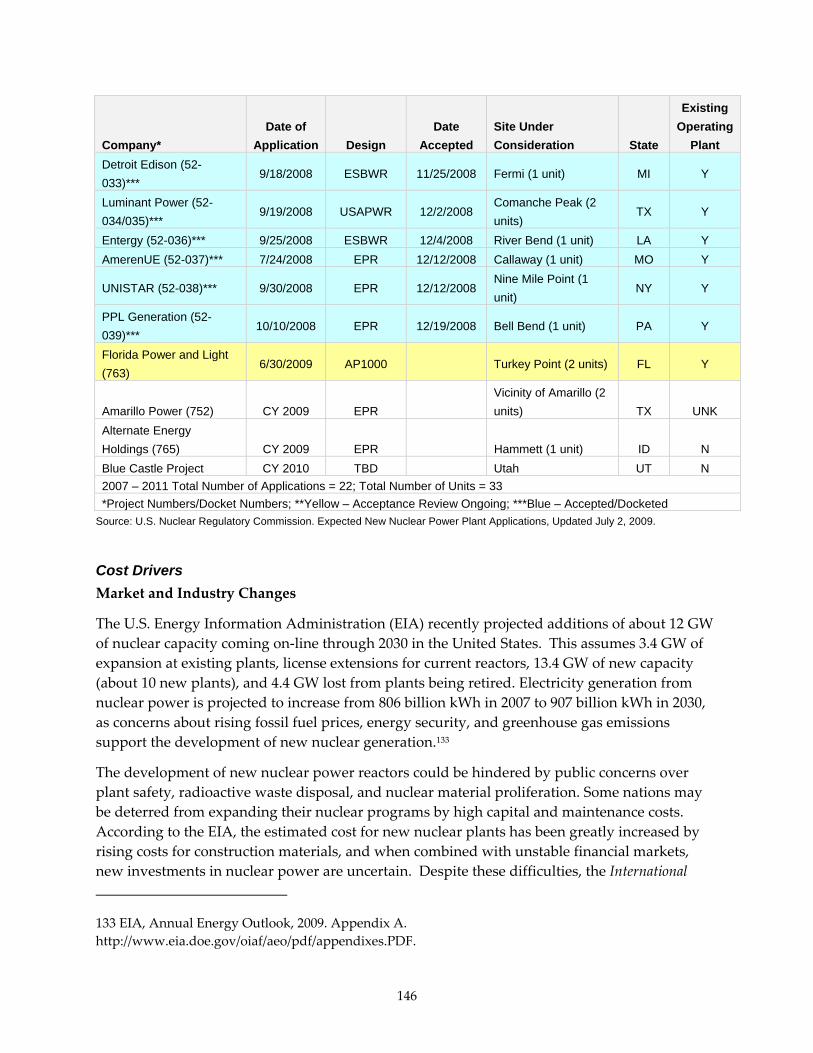
146
Company* Date of
Application Design Date
Accepted Site Under Consideration State
Existing Operating
Plant Detroit Edison (52-033)***
9/18/2008 ESBWR 11/25/2008 Fermi (1 unit) MI Y
Luminant Power (52-034/035)***
9/19/2008 USAPWR 12/2/2008 Comanche Peak (2 units)
TX Y
Entergy (52-036)*** 9/25/2008 ESBWR 12/4/2008 River Bend (1 unit) LA Y AmerenUE (52-037)*** 7/24/2008 EPR 12/12/2008 Callaway (1 unit) MO Y
UNISTAR (52-038)*** 9/30/2008 EPR 12/12/2008 Nine Mile Point (1 unit)
NY Y
PPL Generation (52-039)***
10/10/2008 EPR 12/19/2008 Bell Bend (1 unit) PA Y
Florida Power and Light (763)
6/30/2009 AP1000 Turkey Point (2 units) FL Y
Amarillo Power (752) CY 2009 EPR Vicinity of Amarillo (2 units) TX UNK
Alternate Energy Holdings (765) CY 2009 EPR Hammett (1 unit) ID N Blue Castle Project CY 2010 TBD Utah UT N 2007 – 2011 Total Number of Applications = 22; Total Number of Units = 33 *Project Numbers/Docket Numbers; **Yellow – Acceptance Review Ongoing; ***Blue – Accepted/Docketed
Source: U.S. Nuclear Regulatory Commission. Expected New Nuclear Power Plant Applications, Updated July 2, 2009.
Cost Drivers Market and Industry Changes
The U.S. Energy Information Administration (EIA) recently projected additions of about 12 GW of nuclear capacity coming on‐line through 2030 in the United States. This assumes 3.4 GW of expansion at existing plants, license extensions for current reactors, 13.4 GW of new capacity (about 10 new plants), and 4.4 GW lost from plants being retired. Electricity generation from nuclear power is projected to increase from 806 billion kWh in 2007 to 907 billion kWh in 2030, as concerns about rising fossil fuel prices, energy security, and greenhouse gas emissions support the development of new nuclear generation.133
The development of new nuclear power reactors could be hindered by public concerns over plant safety, radioactive waste disposal, and nuclear material proliferation. Some nations may be deterred from expanding their nuclear programs by high capital and maintenance costs. According to the EIA, the estimated cost for new nuclear plants has been greatly increased by rising costs for construction materials, and when combined with unstable financial markets, new investments in nuclear power are uncertain. Despite these difficulties, the International
133 EIA, Annual Energy Outlook, 2009. Appendix A. http://www.eia.doe.gov/oiaf/aeo/pdf/appendixes.PDF.

147
Energy Outlook 2008 (IEO2008) case incorporates improved prospects for world nuclear power.”134 The IEO2008 projection for nuclear electricity generation in 2025 is 31% higher than the projection published in IEO2003 only five years ago.
Current Trends
Economic and Operating Trends
The industry is concerned about the adequacy of the skilled labor pool and loss of skilled laborers and engineers due to retirement and lack of new graduates seeking careers in nuclear engineering. The lack of skilled nuclear engineers, construction managers with nuclear experience, and skilled tradespeople (boilermakers, pipefitters, electricians, and ironworkers) are a significant bottleneck in nuclear plant construction. Large‐scale revival of nuclear power in the United States will depend on the industry’s approach to these critical labor issues. Already, the NP2010 recommendations contend that nuclear plant designs should be at a complete stage prior to issuance of EPC (engineer‐procure‐construct) contracts, so that labor supply can be properly estimated and managed.135 This recommendation is different than many of the fast track construction methods used today.
One recent trend in the United States’ nuclear power industry that might influence future performance has been an increased concentration of operations into fewer owner‐operators. Concentrated ownership of nuclear reactors began in the 1990s as investor‐owned utilities sought to either eliminate their nuclear risks and the risks of nuclear operating license extensions, or to concentrate those risks into a larger, nuclear‐concentrated business. The effects of industry consolidation into fewer, more specialized nuclear operating companies are illustrated in the table below:
Table 28. Operators of U.S. reactors136
Organization Capacity (MWe) Share of Capacity Exelon-AmerGen 16,850 17.3%
Entergy 9,033 9.2% Duke 6,996 7.2% TVA 6,658 6.8%
Southern 5,698 5.8% 2nd Five Firms 22,680 23.2%
Others (3+ Reactors) 7,164 7.3% Others (<3 Reactors) 22,588 23.1%
Source: www.eia.gov
134 http://www.eia.doe.gov/oiaf/ieo/electricity.html.
135 D’Olier, Robert, et.al. DOE NP2010 Construction Infrastructure Assessment. U.S. Department of Energy, October 2005.
136 http://www.eia.doe.gov/cneaf/nuclear/page/analysis/nuclearpower.html.

148
Ownership percentages are smaller than the operating percentages above because many reactors operate under two sets of agreements: ownership agreements and operating agreements. Entergy and Exelon, both investor‐owned utilities that are pursuing nuclear‐based generation strategies, have both purchased management rights at nuclear plants. Overall, outside of Exelon, there is a roughly 5‐10% share range of capacity exposure that nuclear operators are willing to hold as on balance sheet exposure, and this has led to some leveling out of the top nuclear operators over time.
The data in the table do not include the Stars group, which shares some responsibilities among the managers of many of the smaller managerial groupings.
Capacity uprating, or adding additional generating capacity due to advances in technology in either the power cycle or the turbine‐generator set, has been a continuing trend in nuclear power, as it has also been in other, fossil‐fired technologies. Continuing advances in technology can be used by nuclear plant operators to gain additional megawatt capacity and energy production from the same plant site, as better materials and blade applications come to market.
Typical capacity uprates can increase capacity of existing nuclear reactors approximately 5‐20%.137 EIA estimates the near‐term potential of these uprates around 4 GWe, based on utility and regulatory public announcements. These uprates generally follow the same justification as is done in fossil‐fired generation plant, where the incremental benefit of the uprate exceeds the incremental cost of retrofit and operation, viewed on a lifecycle basis.
Technology Trends
With 443 nuclear power reactors in use worldwide, nuclear generation provides approximately 16% of global electricity generation. Several industrialized countries use nuclear power as a primary source of electricity (Japan, Germany, and France – which produces 78% of its electricity from nuclear power).138 Finland, Japan, Korea and China have active nuclear generation expansion programs underway. Today, the primary reactor embodiments are earlier‐generation technologies known as Generation II reactors, which came on‐line in the 1960s and 1970s. Some limited construction of Generation III reactors has gone into service, primarily in Asia. Most of today’s nuclear rebirth has taken place as a result of the design evolution into advanced reactors known as Generation III+, and the future designs forthcoming as Generation IV reactor technologies.
137 Ibid. [130].
138 IEA/OECD, “IEA Energy Technology Essentials – Nuclear Power.” March 2007.

149
Figure 56. Generations of nuclear energy Source: U.S. DOE and GIF, A Technology Roadmap for Generation IV Nuclear Energy Systems.
With the nuclear industry recovering from virtual stagnation over the last two decades, new factors in the energy landscape have implied a potentially larger role for nuclear power in supplying domestic energy needs. Issues such as global climate change and air quality suggest a future for carbon‐free, emission‐free nuclear technologies, while discussion over energy independence and security also reinforces the hypothesis that growing nuclear power generation in the United States could enhance the energy infrastructure and alleviate security concerns. However, it is clear that without a continued advancing of nuclear technology to reduce overall installed cost relative to fossil‐fueled and other technologies, nuclear power will not enjoy the renaissance many advocates envision.139
To answer these issues and questions, the U.S. Department of Energy has led the development of new, next generation nuclear steam supply systems, known as Generation IV, Generation V, and nuclear fusion reactors. (Fusion reactors as described below are beyond the time frame of this study.)
Generation IV Reactors (not feasible before 2030)
Generation IV reactors are a set of theoretical nuclear reactor designs being researched by a consortium of 10 countries around the world. These designs are generally not expected to be available for commercial construction before 2030, which is beyond the horizon for this study.
139 The Future of Nuclear Power. Massachusetts Institute of Technology, 2003.

150
Today’s commercial reactors are typically of either Generation II or Generation III /III+ technologies, with most Generation I reactors having been retired from service.
In 1999, this consortium of international countries created the Generation IV International Forum (GIF) to research new reactor technologies based on eight fundamental objectives. The primary goals are to: improve nuclear safety, improve proliferation resistance, minimize waste and natural resource use, and to decrease the cost to build and run such plants.140
Several advanced reactor technologies are being evaluated for study, including:141
• Gas‐cooled fast reactor
• Lead‐cooled fast reactor
• Molten salt reactor
• Sodium‐cooled fast reactor
• Supercritical water reactor
• Very‐high‐temperature reactor
Generation V+ Reactors (not feasible before 2030)
Generation V+ reactors are designs that may be theoretically possible but are not being actively considered for commercial development, either because of current technology application potential, or economics, or safety. These technologies include, but are not limited to:
• Liquid core reactor
• Gas core reactor
• Gas core EM reactor
• Fission fragment reactor
Fusion Reactors (not feasible before 2050)
The controlled power of nuclear fusion continues to be an area of active research in nuclear power technology, with the international ITER Tokamak fusion reactor now operational in Europe and scientific research continuing over the next several decades. Fusion of hydrogen isotopes in an ultra‐high‐temperature plasma carries with it the promise of virtually unlimited fuel supply and minimal radioactive waste products, but significant scientific and technical obstacles remain. A study done by the Swiss Federal Institute of Technology for the IEA
140 http://www.gen‐4.org/PDFs/annual_report2007.PDF.
141 U.S. DOE and Nuclear Research Advisory Committee and the Generation IV International Forum A Technology Roadmap for Generation IV Nuclear Energy Systems. Report GIF‐002‐00, December 2002.

151
concluded that fusion reactors could become part of the technology landscape by 2050, but that widescale adoption would not take place until 2050‐2100. 142
Cost Drivers
It is difficult to take into account all aspects that drive costs within a particular nuclear power plant as the aging infrastructure has resulted in numerous one‐time events. To accurately compare the cost of nuclear against other energy sources, this report has considered the following key cost drivers:
1. Capital costs
The Congressional Budget Office (CBO) has identified financing costs as an important cost driver in their report titled Nuclear Power’s Role in Generating Electricity (May 2008).143 Costs associated with initial construction of the plant are heavily influenced by factors such as construction on previously undeveloped land (known as greenfields), refurbishment, and replacements at existing sites and new unit additions at current sites.
For a nuclear plant the construction costs are generally higher than that for other fossil‐fueled or renewable technologies because the buildings must be constructed especially for radiation containment. Redundant safety systems and advanced plant controls are present, adding additional costs. And all equipment, whether piping, valves, electrical equipment, and controls must all be certified to higher design specifications and standards for use in a nuclear power facility. However, nuclear plants do not require the types of post‐combustion scrubbers and air emissions control technologies commonly found in fossil generation to remove sulfur dioxide, nitrogen oxides, and particulate matter.
Instant construction costs were obtained from a variety of research sources, including two MIT studies, research from the OECD‐Nuclear Energy Agency, the IEA, and several other metastudies. The research team also evaluated several recent filings by Florida Power & Light for construction of an AP1000 reactor, and rating agency and investment bank cost estimates. Direct estimates were also obtained by the research team from Westinghouse and General Electric. Not taken into consideration were cost estimates from industry trade groups, as the capital costs outlined by those organizations did not match well with the larger body of knowledge in reported cost data. In any event, the research team notes that the cost spread for nuclear power is wide and somewhat uncertain and will remain so until new reactors are constructed in the United States.
For cost of capital and installed cost calculations a construction period of nine years was used as an average. This period includes siting, environmental impact studies, and licensing application
142 Gnansounou, Edgard and Denis Bedniaguine. “Potential Role of Fusion Power Generation in a Very Long Term Electricity Supply Perspective: Case of Western Europe.” SESE‐V
143 Congress of the United States, Congressional Budget Office. Nuclear Power’s Role in Generating Electricity. May 2008. Retrieved from: http://www.cbo.gov/ftpdocs/91xx/doc9133/05‐02‐Nuclear.PDF.

152
phases and is based on current French data for nuclear plant licensing and construction periods. The nine‐year period is three to four years longer than the timeline recommended by the U.S. Nuclear Regulatory Commission and is based on the research team’s view that the next wave of nuclear plants built in California will be subject to rigorous scrutiny and review. The time estimates of nine‐year construction periods match up well with experience in both the historical context of actual built plant plus current build cycles in Europe.
The nine‐year construction period estimate for nuclear plant construction, combined with utility financing of the nuclear power investment costs throughout the plant’s useful life, means that utilities that construct nuclear power plants must account and plan for the significant increases in financial liquidity to meet the demands of financing a nuclear program. Several financial rating agencies have stated that utilities with nuclear programs should take adequate steps to insure liquidity to avoid rating downgrades.144
2. Fuel costs
Costs associated with the fuel used in the production of energy.
For a nuclear plant, these tend to be lower even though the following steps occur in the production of the fuel assemblies used in the reactor:
1. Mining of the uranium ore145
2. Conversion to U3O8 (uranium oxide ‐ yellowcake form) and then to uranium hexafluoride
3. Enrichment from 0.7% U235 to 2‐5% U235
4. Pelletization into usable uranium dioxide pellets (UO2)
5. Fabrication of pellets into rods, and then fuel assemblies 146
Transportation costs comprising completed uranium fuel assemblies are comparable with coal transportation costs because of the vast amounts of uranium ore required for processing.
3. Operation and maintenance costs
Operation and maintenance costs for a nuclear power station are generally consistent with that of other fossil‐fueled stations, including the costs of:
a) Labor and overheads (e.g., medical and pension benefits).
b) Consumable materials.
c) NRC and state license fees (e.g., license changes, on‐site and regional inspectors, and headquarters staff).
144 Moody’s Investor Services, “New Nuclear Generating Capacity: Potential Credit Implications for U.S. Utilities,” May 2008.
145 http://www.stockinterview.com/News/01092007/Uranium‐Price‐Forecast.html.
146 Tolley, George, et.al. The Economic Future of Nuclear Power. University of Chicago, August 2004.

153
d) Property taxes and insurance, which vary by state and locality.
e) Costs associated with plant outages and replacement/repair of major components.
Additional costs can be levied by the NRC for operating license reviews, or when plants require enhanced inspections following a significant deterioration in plant performance and safety. Also, additional costs can occur for enhanced security needs in the post‐9/11 environment, which are difficult to quantify and are not included in the O&M cost tabulation.
Property taxes can result in a plant paying up to $ 15‐20 million per year in property taxes.
4. Waste‐related costs
For a nuclear plant, these costs include the surcharge levied by the Department of Energy for a nuclear waste fund to pay for the transportation and ultimate disposal of the spent nuclear fuel from reactors as well as costs associated with transportation and disposal of low‐level radioactive wastes. The DOE charge for spent fuel disposal is a flat fee based on energy use. Low‐level waste disposal costs are relatively modest during ongoing plant operations. However, a substantial quantity of low‐level waste will need to be disposed of when the plants are decommissioned.
5. Decommissioning costs
The costs associated with dismantling a shutdown reactor, decontamination, and restoration of the plant site back to greenfield status. Usually restoration would occur over a long period, e.g. 20 years. Parts of the plant (e.g., non‐nuclear plant components) could be used for energy generation by other sources.
In California, PG&E, SCE, and San Diego Gas & Electric (SDG&E) collect about 0.03 cents/kWh from retail rates to fund decommissioning. They must then report regularly to the NRC on the status of their decommissioning funds. As of 2001, $23.7 billion of the total estimated cost of decommissioning all United States’ nuclear power plants had been collected, leaving a liability of about $11.6 billion to be covered over the operating lives of 104 reactors (on basis of average $320 million per unit).
The projected United States’ industry average cost for decommissioning a power plant is $300 million. The funds for this activity are accumulated in the operating cost of the plant. The French and Swedish Nuclear Industries expect decommissioning costs to be 10 ‐15 % of the construction costs and budget this into the price charged for electricity. On the other hand the British decommissioning costs have been projected to be around 1 billion pounds per reactor. 147 In California, according to SCE, for SONGS 2 and 3, estimated decommissioning costs are $3.659
147 http://nuclearinfo.net/Nuclearpower/WebHomeCostOfNuclearPower

154
billion in 2008 dollars, and for SONGS 1, the estimate is $769.2 million. Rancho Seco’s decommissioning costs were estimated to be $518 million (2002 dollars).148
Examples of several nuclear reactors dismantled in America, type, power, and decommissioning cost (often is mentioned only the probable cost per kilowatt of power):
Table 29. Nuclear decommissioning costs149
Country Location Reactor type Operative
Life Decommissioning
Phase Dismantling
Costs:
U.S. Fort St. Vrain
High temperature, gas-cooled
reactor (HTGR) [helium-graphite] 380 MWe
12 years (1977-1989)
Immediate Decon $ 195 Million
U.S. Maine Yankee PWR
860 MWe
24 years (closed in
1996)
DECON COMPLETED - Demolished in
2004 (greenfield open to
visitors)
$ 635 Million
U.S. Connecticut
Yankee PWR
590 MWe
28 years (closed in
1996)
Decon - demolished in
2007 (greenfield open to
visitors)
$ 820 Million
Source: http://nuclearinfo.net
Current Costs Installation Costs
The summarized low/average/high costs are based on several research and financial sources (Keystone Center and Moody’s Investor Service) as well as on the data provided by the major operators of the nuclear power plants (Florida Power & Light, Georgia Power and South Carolina Electric and Gas Company). These major owners and 27 other nuclear power companies/contractors have concluded in June 2007 that the cost for building new reactors would be between $3,600 and $4,000 per installed kW (with interest). They also projected that the operating costs for these plants would be remarkably expensive: $0.30/kWh for the first 13 years until construction costs are paid followed by $0.18/kWh over the remaining lifetime of the
148 Byron, Barbara, Research Team Communication with California Energy Commission Staff
149 http://nuclearinfo.net/Nuclearpower/WebHomeCostOfNuclearPower

155
plant. Just a few months later, in October 2007, Moody’s Investor Service projected even higher costs due to the quickly escalating price of metals, forgings, other materials, and labor needed to construct reactors. They estimated total costs for new plants, including interest, at between $5,000 and $6,000 per installed kW. Florida Power & Light informed the Florida Public Service Commission in December 2007 that its estimated cost for building two new nuclear units at Turkey Point in South Florida was $8,000 per installed kW. Based on the rapidly changing nature of these cost estimates, and their resultant uncertainty, additional data sources were located because of the recent changes in installed cost estimates since 2007, which increased overall cost estimates used in this study. Moody’s Investor Service recently updated its estimates for nuclear construction costs, indicating that construction costs are now projected at $7,000 per installed kW. 150 A recent study by Cooper details the rising trend in nuclear power construction costs and the widespread between estimates over recent years.151
Included in the installation/construction costs are: cooling towers, site works, transmission costs and risk management, plant components, project financing costs, license application, regulatory fees, initial fuel, insurance and taxes, escalation, and contingencies.
Financial Cost of Construction
The research team included costs for Allowance for Funds Used During Construction (AFUDC) in the preliminary analysis. The allowance for funds used during construction calculation, especially for nuclear plant construction, can be highly variable and is based on the total duration from plant inception to declaration of commercial operation.152 While most sources, including the NRC, assume a construction spending profile of five years (60 months) duration, with pre‐construction periods of 18 months, actual plant construction of 36 months, and start‐up operations commissioning of 6 months, the research team lengthened the construction durations to reflect conditions and concerns in current reactor licensing efforts.
The research team concluded that reasonable basis for licensing and construction planning would be the experience seen in France, where there is considerable time spent in pre‐construction phase plant licensing, permitting and study evaluations. This additional time lengthens the overall construction period to 8‐10 years, and the research team used a construction period of nine years duration, and a construction spending profile as shown in the following table:
150 Ibid. 144: 151 Mark Cooper, “The Economics of Nuclear Reactors: Renaissance or Relapse,” Vermont Law School, June 2009.
152 Organisation for Economic Co‐operation and Development. Projected Costs of Generating Electricity: 2005 Update. OECD Nuclear Energy Agency, International Energy Agency, 2005.

156
Table 30. Nuclear plant construction spending profile (% of total instant cost per year)
Year 1 2 3 4 5 6 7 8 9 % total
instant cost 2.5 2 7 15.5 22 21 18 10 2
Source: OECD Nuclear Energy Agency, International Energy Agency, Organisation for Economic Co-operation and Development. Projected Costs of Generating Electricity: 2005 Update. OECD Publishing, 2005
The first three years are the cash flow spending projections used for pre‐construction permitting, licensing, and environmental studies and approvals. Following approvals, the next six years is a spending profile consistent with the actual construction, start‐up, commissioning, and testing of the nuclear plant.
Because of the minimal recent experience in nuclear plant licensing and approvals, the research team believes that a utility will devote significant time and efforts into the pre‐construction licensing process. Three years duration is reasonable for additional site licensing, studies, and environmental impact findings leading to planning and regulatory approvals needed to begin actual construction. While the research team notes that the procurement method for nuclear power in France concentrates authority in a triumvirate between government, a government‐sponsored utility, and a standard design, the choice of a nine‐year construction duration is transferable to the United States and to California because of the historical track record of construction durations in this country, the concentration of the nuclear industry into an oligopoly of few commercial providers, and the increasing demand of the financial and utility industries for federal loan guarantees for nuclear plant. All of these coincident forces create an environment similar to current French experience.
Notable in the derivation of AFUDC for the nuclear case, the research team assumed that the interest rate, and thus the cost of funds, would be that of an investor‐owned utility, and not that of a merchant generator or a public owned utility.
Expected Cost Trajectories Expected cost trajectories for nuclear power options are expected to rise nominally with inflation, and only little experience curve effects, even based on the new Generation IV reactor designs. The lack of sufficient momentum in increasing the cumulative generation capacity represented by nuclear plants and the mature experience curve of the nuclear power industry caused the research team to model experience curve effects at a 95% rate (doubling of the installed capacity represents a 5% cost decrease due to experience).
Nominally, the research team expects that nuclear cost trajectories will rise at a rate greater than inflation as the new Generation IV reactors are begun. As new Generation IV reactors are built over the next several years and instant/installed cost ranges tighten, the research team expects nuclear escalation rates higher than normal cost inflation, but moderating in the 2018‐2030 time period as follows:
• High Case: Additional 7% escalation through 2018, then additional 5% through 2030:
• Average Case: Additional 5% escalation through 2018, then additional 3% through 2030:
• Low Case: Additional 3% escalation through 2018, then nominal inflation through 2030.

157
4.0 Conclusions and Recommendations
KEMA performed a detailed assessment of the technologies that are likely to be deployed in the next 20 years. For each technology, KEMA conducted a quantitative and qualitative assessment of cost drivers and trends to develop input variables for the California Energy Commission’s levelized cost model. KEMA performed a detailed literature review to support this study and identified utility‐scale renewable energy and two non‐renewable energy technologies that may likely be deployed in California over the next 20 years, along with identification of the infrastructure scales at which they are likely to be deployed.
For each technology, KEMA identified cost drive drivers and trends contributing to technology deployment and performed a quantitative assessment of factors to determine high, average, and low estimates of expected costs. In addition, KEMA has developed a detailed assessment of the expected trajectories for future costs for utility‐scale generation. KEMA’s research led to the development of detailed cost sheets that provide the input variables for the Commission’s levelized cost analysis. The final project report will also address community and building‐scale technologies as well as summarize key findings and recommendations.
Future cost of generation studies should consider including:
• Qualitative or quantitative assessment of other key issues that may influence costs of generation including:
ο CO2 abatement costs ο Environmental sensitivity ο Land‐use constraints ο Permitting risk ο Transmission constraints and equity issues related to who bears the cost of new
transmission ο System integration costs ο System diversity ο Tax credit availability and structure ο Financing availability ο Macro‐economic benefits (jobs creation, security, fuel diversity, etc.) ο Natural gas price and wholesale price effects associated with increased
penetration of renewables ο Carbon capture and storage ο Storage (CAES, Battery, Pumped Hydro) ο Dispatchability analysis ο Other risk factors
• More time for a stakeholder input similar to the RETI process or CPUC GHG Modeling Initiatives.

158

159
5.0 References
Abrams, Richard F. and Kevin Toupin. “Efficient and Low Emission Stoker Fired Biomass Boiler Technology in Today’s Marketplace.” POWER‐GEN Renewable Conference Technical Publication, March 2007.
Beurskens, L.W.M., M. de Noord, and H.J. de Vries. Potentials and Costs for Renewable Electricity Generation. Energy Research Centre of the Netherlands. ECN‐C–03‐006, February 2004.
Black & Veatch. Clean Coal Technology Selection Study Final Report January 2007. Black & Veatch, 2007.
Black & Veatch. Renewable Energy Transmission Initiative Phase 1A (Draft Report). Black & Veatch, RETI Stakeholder Steering Committee, Project Number 149148.0010, March 2008. http://www.energy.ca.gov/2008publications/RETI‐1000‐2008‐001/RETI‐1000‐2008‐001‐D.PDF.
Black & Veatch. Technical Analysis of the Energy Resource. Black & Veatch Project: 144864, October 2007.
Breeze, Paul. The Cost of Power Generation: The Current and Future Competitiveness of Renewable and Traditional Technologies. Business Insights Ltd., 2008. http://www.globalbusinessinsights.com/content/rben0202m.PDF.
California Public Utility Commission. Generation Costs 2008, CPUC, 2007. http://www.ethree.com/GHG/Generation%20costs.doc
Christoua, Costas, Ioannis Hadjipaschalisa and Andreas Poullikkas. “Assessment of Integrated Gasification Combined‐Cycle Technology Competitiveness.” Renewable and Sustainable Energy Reviews 12, Issue 9, (December 2008): 2459‐2471.
Chupka, Marc W. and Gregory Basheda. Rising Utility Construction Costs: Sources and Impacts. The Edison Foundation, September 2007.
Cobb, James T. “Survey of Commercial Biomass Gasifiers.” University of Pittsburgh, AIChE Annual Meeting, November 2007.
Conner, Alison M., Ben N. Rinehart, and James E. Francfort. See U.S. Department of Energy. Idaho National Laboratory.
CPUC, Aspen, E3, and Plexos. “33% Implementation Analysis Working Group Meeting.” 2009.
DeFusco, John, Phillip McKenzie, and Michael Fick. “Bubbling Fluidized Bed or Stoker – Which is the Right Choice for Your Renewable Energy Project.” CIBO Fluid Bed Combustion XX Conference, May 2007.

160
European Photovoltaic Technology Platform. A Strategic Research Agenda for Photovoltaic Solar Energy Technology. European Photovoltaic Technology Platform, 2007. http://cordis.europa.eu/technology‐platforms/pdf/photovoltaics.PDF.
Gray, David. See U.S. Department of Energy. Office of Coal and Environmental Systems Gasification Technologies Program.
Hall, Douglas G. and Kelly S. Reeves. See U.S. Department of Energy. Idaho National Laboratory.
Hall, Douglas G., Richard T. Hunt, Kelly S. Reeves, and Greg R. Carroll. See U.S. Department of Energy. Idaho National Laboratory.
Hance, Cedric. Factors Affecting Costs of Geothermal Power Development. Geothermal Energy Association, August 2005.
Haq, Zia. See Biomass for Electricity Generation. U.S. Department of Energy. Energy Information Administration, 2002.
International Energy Agency. Experience Curves for Energy Technology Policy. Organization of Economic Cooperation and Development (OECD), 2000.
Kagel, Alyssa. A Handbook on the Externalities, Employment, and Economics of Geothermal Energy. Geothermal Energy Association, October 2006.
Kaplan, Stan. Power Plants: Characteristics and Costs. Congressional Research Service. National Council on Science and the Environment, Washington DC, 2008.
Klein, Joel and Anitha Rednam. “Comparative Costs of California Central Station Electricity Generation Technologies.” California Energy Commission, Electricity Supply Analysis Division, CEC‐200‐2007‐011, December 2007. http://www.energy.ca.gov/2007publications/CEC‐200‐2007‐011/CEC‐200‐2007‐011‐SF.PDF.
Koetzier, H, FJJM van Aart, PJ Ploumen, PH Wakker, and HC Wels. Update technische review grootschalige elektriciteitsopwekking. KEMA, 2007.
Lenardic, Denis. Large‐Scale Photovoltaic Power Plants: Cumulative and Annual Installed Power Output Capacity, Annual Report 2007. pvresources.com, Revised Edition, April 2008. http://www.pvresources.com/download/AnnualReport2007.PDF.
Minchener, AJ. “Coal Gasification for Advanced Power Generation.” Fuel 47, Issue 3, May 2006: 171.
National Energy Renewable Energy Laboratory. Assessment of Parabolic Trough and Power Tower Solar Technology Cost and Performance Forecasts. NREL/SR‐350‐34440, October 2003.
O’Connell, Ric, and Ryan Pletka, et al. 20 Percent Wind Energy Penetration in the United States: A Technical Analysis of the Energy Resource. Black & Veatch Project: 144864, October 2007. 5‐10.

161
Overend, Ralph P. Biomass Conversion Technologies. Golden, CO: National Renewable Energy Laboratory, March 2007.
Purchasing Magazine. “Steel Plate Prices Have Plunged 50% From Mid‐2008 Peak.” Purchasing Magazine. April 2009. www.purchasing.com/article/CA6654110.html?industryid=48389.
Rhodes, James S. and DavidW. Keith. “Engineering Economic Analysis of Biomass IGCC With Carbon Capture and Storage.” Biomass and Bioenergy 29 (2005): 440‐450.
Rosenberg, William G., Dwight C. Alpern, and Michael R. Walker. “Deploying IGCC Technology in this Decade with 3 Party Covenant Financing: Volume II.” ENRP Discussion Paper 2004‐07: Belfer Center for Science and International Affairs, Kennedy School of Government, Harvard University, Cambridge, MA, July 2004.
Sison‐Lebrilla, Elaine, Valentino Tiangco. Geothermal Strategic Value Analysis. CEC‐500‐2005‐105‐SD, June 2005.
Solar Millenium. Nevada Energy, Solar Millennium and MAN Ferrostaal cooperate in the development of projects. Solar Millenium Corporate News, April 3, 2009. http://www.solarmillennium.de/Press/Press_Releases/Nevada_Energy__Solar_Millennium_and_MAN_Ferrostaal_cooperate_in_the_development_of_projects,lang2,50,1532.html.
Stahl, Krister, Lars Waldheim, Michael Morris, Ulf Johnsson, and Lennart Gårdmark. “Biomass IGCC at Varnamo, Sweden – Past and Future.” GCEP Energy Workshop, April 2004.
Stoddard, L., J. Abrecunas, and R. O’Connell. Economic, Energy, and Environmental Benefits of Concentrating Solar Power in California. National Renewable Energy Lab, NREL/Sr‐550‐39291, April 2006.
Tavoulareas, Stratos. Advanced Power Generation Technologies – An Overview. U.S. Agency for International Development. ECO‐Asia Clean Development Program, August 2008.
Thorpe, Tom. A Brief Review of Wave Energy. AEA Technology. ETSU‐R120, May 1999.
U.S. Department of Energy. Energy Efficiency and Renewable Energy (EERE). 20% Wind Energy by 2030, Increasing Wind Energy’s Contribution to U.S. Electric Supply. DOE/GO‐102008‐2567, July 2008.
U.S. Department of Energy. Energy Information Administration, Biomass for Electricity Generation, by Zia Haq, 2002.
U.S. Department of Energy. Energy Information Administration. Annual Energy Outlook 2009 (AEO2009). DOE/EIA‐0383(2009), March 2009.
U.S. Department of Energy. Energy Information Administration. Electric Power Annual 2007. DOE/EIA‐0348(2007), January 2009. http://www.eia.doe.gov/cneaf/electricity/epa/epa_sum.html.

162
U.S. Department of Energy. Energy Information Administration. Assumptions to the Annual Energy Outlook 2008, With Projections for 2030. DOE/EIA‐0554(2008), June 2008. http://www.eia.doe.gov/oiaf/archive/aeo08/assumption/pdf/0554(2008).PDF.
U.S. Department of Energy. Energy Information Administration. Electricity Market Module (EMM). DOE/EIA‐0554(2009), March 2009.
U.S. Department of Energy. Idaho National Laboratory. A Study of United States Hydroelectric Plan Ownership, by Douglas G. Hall, and Kelly S. Reeves. INL/EXT‐06‐11519, June 2006.
U.S. Department of Energy. Idaho National Laboratory. Estimation of Economic Parameters of U.S. Hydropower Resources, by Douglas G., Hall, Richard T. Hunt, Kelly S. Reeves, and Greg R. Carroll. Bechtel BWXT Idaho LLC and INL Hydropower Resource Economics Database, June 2003.
U.S. Department of Energy. Idaho National Laboratory. U.S. Hydropower Resource Assessment for California, by A. M. Conner, B. N. Rinehart, and J. E. Francfort. DOE/ID‐10430(CA), October 1998.
U.S. Department of Energy. National Energy Technology Laboratory. Cost and Performance Baseline for Fossil Energy Plants. DOE/NETL‐2007/1281, August 2007. http://www.netl.doe.gov/energy‐analyses/pubs/Bituminous%20Baseline_Final%20Report.PDF.
U.S. Department of Energy. Office of Coal and Environmental Systems Gasification Technologies Program. Current and Future IGCC Technologies: Bituminous Coal to Power, by David, Gray, Salvatore Salerno, and Glen Tomlinson, 2004.
U.S. Department of Energy. Office of Fossil Energy. National Energy Technology Laboratory. Gasification World Database 2007, October 2007. <http://www.netl.doe.gov/technologies/coalpower/gasification/database/database.html>.
U.S. Environmental Protection Agency. Combined Heat and Power Partnership. Biomass Combined Heat and Power Catalog of Technologies, September 2007.
U.S. Environmental Protection Agency. Environmental Footprints and Costs of Coal‐Based Integrated Gasification Combined‐Cycle and Pulverized Coal Technologies. EPA‐430/R‐06/006, July2006. http://www.epa.gov/air/caaac/coaltech/2007_01_epaigcc.PDF.
Van Dam, Case P. Wind Power Generation Trends at Multiple California Sites. California Energy Commission. Publication Number: CEC‐500‐2005‐185, December 2005.
Wiser, Ryan and Mark Bolinger. Annual Report on U.S. Wind Power Installation, Cost, and Performance Trends: 2007. U.S. Department of Energy. EERE, May 2008.

163
URLs Cited:
Abengoa Solar: http://www.abengoasolar.com
California Energy Commission: http://www.energy.ca.gov/ (California Energy Commission)
CRU Steel Price Index (CRUspi): http://cruonline.crugroup.com/SteelFerroalloys/CRUSteelPrices/CRUspi/tabid/143/Default.aspx
DLR (German Aerospace Center): http://www.dlr.de
Dutch Association of Cost Engineers: http://www.dace.nl/
Energy Information Administration: http://www.eia.doe.gov/
Energy Products of Idaho: http://www.energyproducts.com/
European PhotoVoltaic Industry Association: http://www.epia.org/
juwi (sustainable energy web site in German): www.juwi.de
National Renewable Energy Laboratory: http://www.nrel.gov/
Network of National PV Associations: http://nnpva.net/
NOBESOL (PV services web site in Spanish): www.nobesol.com
Nuclear Power Education: http://nuclearinfo.net/Nuclearpower/WebHomeCostOfNuclearPower
Oregon Institute of Technology: http://geoheat.oit.edu/directuse/power.htm
Photon: das Solarstrom‐Magazin: http://www.photon.de/
Solar Millennium AG: http://www.solarmillennium.de
SolarBuzz–Portal to the World of Solar Energy: http://www.solarbuzz.com/
Solarwirtschaft ‐ Official Homepage of the German Solar Industry Association: http://www.solarwirtschaft.de/ Solarwirtschaft ‐ Official Homepage of the German Solar Industry Association.
SunPower: www.sunpowercorp.com
Technical Service Center: http://www.usbr.gov/pmts/estimate/cost_trend.html.
U.S. DOE Energy Efficiency and Renewable Energy: http://www.eere.energy.gov/ (U.S. DOE Energy Efficiency and Renewable Energy)
Westinghouse: http://www.ap1000.westinghousenuclear.com.

164
Nuclear cost references:
Comparison of Fuel, Operations and Maintenance, and Capital Costs as a function of Unit Capacity Factor. http://www.nucleartourist.com/basics/cost‐comparison.htm
Corradini, Mike. “Nuclear Power: Prospects in the 21st Century” Wisconsin Institute of Nuclear Systems. http://www.energy.wisc.edu/presentations/
King, Jeff. “Sixth Northwest Conservation & Electric Power Plan, Proposed Nuclear Power Plant Planning Assumptions.” Northwest Power and Conservation Council, Generating Resources Advisory Committee, Portland, OR, October 23, 2008. http://www.nwcouncil.org/energy/grac/meetings/2008/10/Nuclear%20planning%20assumptions%20‐%206P%20Draft%20102208.ppt
Klein, Joel and Anitha Rednam. Comparative Costs of California Central Station Electricity Generation Technologies. California Energy Commission, Electricity Supply Analysis Division, CEC‐200‐2007‐011, December 2007. http://www.energy.ca.gov/2007publications/CEC‐200‐2007‐011/CEC‐200‐2007‐011‐SF.PDF.
Lacruz, Jeffrey. “Discussion of various plant types and cost comparison.” Technical Background Report (partial report). http://www.io.com/~hcexres/textbook/finrepx7c.html.
New York & Washington Nuclear Comporations. “Nuclear Fuel Prices.” http://www.nynco.com/html/nuclear_fuel_prices.html
NRC Cost Comparison (note‐NRC costs do not reflect decommissioning, capital, waste costs). http://www.nrc.gov/NRC/NUREGS/SR1350/V9/part07.html
Nuclear Energy Institute. “Cost and Performance.” http://www.nei.org/library/infob1.htm
Paulson, Keith. “Future Commercial Nuclear Power Expansion in the US.” World Nuclear Association Annual Symposium. London, 4‐6 September 2002. http://www.world‐nuclear.org/sym/2002/pdf/paulson.PDF.
Smith‐Kevern, Rebecca. “Advanced Reactors and Government Support for New Nuclear Plants.” Presentation to the National Association of Regulated Utility Commissioners. February 2008. www.narucmeetings.org/Presentations/Smith‐Kevern.ppt
Uranium Exchange (Ux) Company. “Prices.” http://www.uxc.com/top_review.html
Westinghouse AP1000 Design Control Document Rev. 16 (Public Version). http://adamswebsearch2.nrc.gov/idmws/ViewDocByAccession.asp?AccessionNumber=ML071580939

165
Levelized Cost Estimates:
“Business Energy Tax Credit (BETC).” http://www.oregon.gov/ENERGY/CONS/BUS/docs/Rule_summary.PDF.
Energy and Environmental Analysis, Inc. “Update on EEA Activities for ORNL/DOE DG/CHP Program.” October 2004. http://www.intermountainchp.org/initiative/support/eea041013.PDF.
Energy Information Administration. “Federal Energy Market Interventions 1999: Primary Energy.” http://www.eia.doe.gov/oiaf/servicerpt/subsidy/pdf/appendix_b.PDF.
Ford, F. Peter. “Technical and Management Challenges Associated with Structural Materials Degradation in Nuclear Reactors in the Future.” Abstract. http://www.cns‐snc.ca/CNS_Conferences/Deg2007/13thPlenaryPaperFinalAug15th.PDF.
Kittler, Ronny. “Renewable Energy in the USA: Federal and State Activities to Promote Alternative Electricity Generation.” Heinrich Böll Foundation. Policy Paper No. 21, April 2003. http://www.boell.org/docs/Renewable_Energy_Final.pdf, REPTC programs
Klein, Joel and Anitha Rednam. Comparative Costs of California Central Station Electricity Generation Technologies. California Energy Commission, Electricity Supply Analysis Division, CEC‐200‐2007‐011, December 2007. http://www.energy.ca.gov/2007publications/CEC‐200‐2007‐011/CEC‐200‐2007‐011‐SF.PDF.
Parker, Larry and Mark Holt. “Nuclear Power: Outlook for New U.S. Reactors.” CRS Report for Congress. Order Code RL33442, March 2007. http://www.fas.org/sgp/crs/misc/RL33442.PDF.
Paul, Anthony. “Electricity Policy Interactions: Climate, Renewables, & Demand Efficiency.” 36th Annual PURC Conference, University of Florida, Gainesville, FL, February 5, 2009. http://www.cba.ufl.edu/purc/docs/presentation_2009Paul.PDF.
Public Service Company of Colorado. “2007 Colorado Resource Plan.” CPUC Docket No. 07A‐447E, December 2008. http://www.xcelenergy.com/SiteCollectionDocuments/docs/CRPGenericCostTables.PDF.
Westinghouse Electric Company “Technology Fact Sheet: Westinghouse – AP1000.” http://www.energetics.com/pdfs/nuclear/ap1000.PDF.

166

167
6.0 Glossary
ABWR Advanced boiling water reactor
AC Alternating current
AEA Association for Educational Assessment (Europe)
AEO Annual Energy Outlook
AFUDC Allowance for funds used during construction
APS Arizona Public Service
ASU Air separation unit
AWEA American Wind Energy Association
BOP Balance of plant
BOS Balance of systems
Btu British thermal unit
BWR Boiling water reactors
California ISO California Independent System Operator
CBO Congressional Budget Office
CCS Carbon capture and sequestration
CFB Circulating fluidized bed
CIBO Council of Industrial Boiler Owners
CO Carbon monoxide
CO2 Carbon dioxide
COG Cost of generation
COL Construction and operation
CPUC California Public Utilities Commission
CREZ Competitive Renewable Energy Zone
CSP Concentrating Solar power
DC Direct current
DOE Department of Energy

168
EAO Electricity analysis office
EERE Energy Efficiency and Renewable Energy
EIA Energy Information Administration
EM Environmental management
EPRI Electric Power Research Institute
ETSU Energy Technology Support unit
EU European Union
EWEA European Wind Energy Association
FB Fluidized bed
FERC Federal Energy Regulatory Commission
FPV Flat‐plate photovoltaic
GADS Generating Availability Data System
GDP Gross domestic product
GE General electric
GeothermEx GeothermEx, Inc.
GHG Greenhouse gas
GIF GEN IV International Forum
GIF Generation International Forum
GW Gigawatt
GWe Gigawatt electric
GWh Gigawatt hour
HCE Heat collec tion element
Hetch Hetchy Hetch Hetchy Water and Power Division
HGTR High temperature gas‐cooled reactor
HPRA Hydroelectric Resource Assessment
IEPR Integrated Energy Policy Report
IGCC Integrated gasification combined‐cycle
INEEL Idaho National Engineering and Environmental Laboratory

169
INL Idaho National Laboratory
IPP Independent power provide
ITC Investment tax credit
kW kilowatt
kWe Kilowatt electric
kWp Kilowatt peak
LBNL Lawrence Berkeley National Laboratory
m meter
MW Megawatt
MWe Megawatt electric
MWh Megawatt hour
MWp Megawatt peak
NERC North American Energy Reliability Corporation
NOx Nitrogen oxide
NRC Nuclear Regulatory Commission
NRE Non‐renewable energy
NREL National Renewable Energy Laboratory
NSPS New Source Performance Standards
O&M Operation and maintenance
OECD Organization of Economic Cooperation and Development
OWC Oscillating water column
PBMR Pebble bed modular reactor
PCFB Pressurized circulating fluidized bed
PG&E Pacific Gas and Electric
PGC Public goods charge
PHWR Pressurized heavy water reactor
PIER Public Interest Energy Research
PPA Power purchase agreement

170
PTC Production tax credit
PURPA Public Utility Regulatory Policies Act
PV Photovoltaic
PWR Pressurized water reactors
RDF Refuse derived fuel
RE Renewable energy
REP Renewable energy program
RETI Renewable Energy Transmission Initiative
RPS Renewables Portfolio Standard
RSCR Riley selective catalytic reduction™
S&L Sargent and Lundy
SCE Southern California Edison
SCR Selective catalytic reduction
SDG&E San Diego Gas & Electric
SFPUC San Francisco Public Utilities Commission
SOx Sulfur dioxide
SRA Strategic research agenda
U.S. United States
UBC Unburned carbon
Unocal Union Oil Company of California
USGS United States Geological Survey
Ux Uranium exchange
WECC Western Electricity Coordinating Council

APPENDIX A
Cost Data

Technology Name: Biomass Combustion - Fluidized Bed BoilerAll costs are in 2009 nominal dollars unless otherwise noted.
Year=2009, Value & DollarsPLANT DATA Average High LowGross Capacity (MW) 28 15 70Station Service (%) 6.00% 7.00% 5.00%Net Capacity (MW) 26.32 13.95 66.50Net Energy (GWh) 196 92 524Transformer Losses 0.50% 0.50% 0.50%Tranmission losses 5.00% 5.00% 5.00%Load Center Delivered Capacity (MW) 24.88 13.19 62.86Net Capacity Factor (NCF) 85.00% 75.00% 90.00%Planned Percent of Year Operational 92.39% 88.65% 97.70%Average Percent Output 100.0% 100.0% 100.0%Net Energy Delivered to Load Center (GWh) 185.25 86.63 495.58Forced Outage Rate (FOR) 8.00% 10.00% 6.00%Scheduled Outage Factor (SOF) 3.00% 6.00% 2.00%Curtailment (Hours) 60 120 0Degradation Factors Capacity Degradation (%/Year) 0.10% 0.20% 0.00% Heat Rate Degradation (%/Year) 0.15% 0.20% 0.10%Emission Factors NOX (lbs/MWh) 0.074 0.074 0.074 VOC/ROG (Lbs/MWh) 0.009 0.009 0.009 CO (Lbs/MWh) 0.079 0.079 0.079 CO2 (lbs/MWh) 0.000 0.000 0.000 SOX (lbs/MWh) 0.020 0.020 0.020 PM10 (lbs/MWh) 0.100 0.200 0.025

Technology Name: Biomass Combustion - Fluidized Bed BoilerAll costs are in 2009 nominal dollars unless otherwise noted.
Start Year 2009 2010 2011 2012 2013 2014 2015 2016 2017 2018 2019PLANT COST DATA Average 1 1 1 1 1 1 1 0.998957181 0.994689784 0.993153861 0.991454788 Instant Cost (Nominal $/Gross MW) $3,200,000 $3,260,838 $3,322,833 $3,386,006 $3,450,380 $3,515,978 $3,582,823 $3,647,132 $3,700,595 $3,765,127 $3,830,145 Installed Cost (Nominal $/Gross MW) $3,580,264 $3,648,331 $3,717,693 $3,788,373 $3,860,397 $3,933,790 $4,008,579 $4,084,790 $4,162,449 $4,241,585 $4,322,225 % Cost of last year of construction 80% 80% 80% 80% 80% 80% 80% 80% 80% 80% 80% % Cost next to last year of construction 20% 20% 20% 20% 20% 20% 20% 20% 20% 20% 20% % Cost of previous year of construction High 1 1 1 1 1 1 1 1.000502406 1.002566461 1.00331257 1.004139926 Instant Cost (Nominal $/Gross MW) $4,800,000 $4,891,257 $4,984,249 $5,079,009 $5,175,570 $5,273,967 $5,374,235 $5,479,161 $5,594,848 $5,705,459 $5,818,725 Installed Cost (Nominal $/Gross MW) $5,810,868 $5,921,344 $6,033,919 $6,148,635 $6,265,532 $6,384,652 $6,506,036 $6,629,728 $6,755,771 $6,884,211 $7,015,092 % Cost first year of construction 60% 60% 60% 60% 60% 60% 60% 60% 60% 60% 60% % Cost second year of construction 40% 40% 40% 40% 40% 40% 40% 40% 40% 40% 40% % Cost third year of construction 0% 0% 0% 0% 0% 0% 0% 0% 0% 0% 0% Low 1 1 1 1 1 1 1 0.997391042 0.98675735 0.982946811 0.978741818 Instant Cost (Nominal $/Gross MW) $1,600,000 $1,630,419 $1,661,416 $1,693,003 $1,725,190 $1,757,989 $1,791,412 $1,820,707 $1,835,542 $1,863,216 $1,890,517 Installed Cost (Nominal $/Gross MW) $1,677,000 $1,708,883 $1,741,372 $1,774,479 $1,808,215 $1,842,592 $1,877,623 $1,913,320 $1,949,696 $1,986,764 $2,024,536 % Cost first year of construction 100% 100% 100% 100% 100% 100% 100% 100% 100% 100% 100% % Cost second year of construction % Cost third year of construction
Start Year 2020 2021 2022 2023 2024 2025 2026 2027 2028 2029PLANT COST DATA Average 0.990617574 0.990357064 0.989558753 0.989219936 0.988245127 0.987627424 0.986618608 0.98506456 0.983981645 0.982000994 Instant Cost (Nominal $/Gross MW) $3,899,668 $3,972,763 $4,045,029 $4,120,521 $4,194,722 $4,271,800 $4,348,568 $4,424,263 $4,503,420 $4,579,801 Installed Cost (Nominal $/Gross MW) $4,404,399 $4,488,135 $4,573,462 $4,660,412 $4,749,016 $4,839,303 $4,931,307 $5,025,061 $5,120,596 $5,217,948 % Cost of last year of construction 80% 80% 80% 80% 80% 80% 80% 80% 80% 80% % Cost next to last year of construction 20% 20% 20% 20% 20% 20% 20% 20% 20% 20% % Cost of previous year of construction High 1.004548377 1.004675576 1.005065676 1.005231382 1.005708603 1.006011363 1.006506426 1.007270524 1.007804031 1.008782067 Instant Cost (Nominal $/Gross MW) $5,931,762 $6,045,301 $6,162,625 $6,280,824 $6,403,272 $6,526,975 $6,654,337 $6,785,996 $6,918,673 $7,057,052 Installed Cost (Nominal $/Gross MW) $7,148,462 $7,284,368 $7,422,857 $7,563,979 $7,707,785 $7,854,324 $8,003,649 $8,155,814 $8,310,871 $8,468,876 % Cost first year of construction 60% 60% 60% 60% 60% 60% 60% 60% 60% 60% % Cost second year of construction 40% 40% 40% 40% 40% 40% 40% 40% 40% 40% % Cost third year of construction 0% 0% 0% 0% 0% 0% 0% 0% 0% 0% Low 0.976673797 0.976030843 0.974062145 0.973227317 0.970827833 0.969309203 0.966832089 0.963023621 0.960375082 0.955542238 Instant Cost (Nominal $/Gross MW) $1,922,388 $1,957,647 $1,990,842 $2,026,953 $2,060,396 $2,096,284 $2,130,679 $2,162,635 $2,197,690 $2,228,202 Installed Cost (Nominal $/Gross MW) $2,063,026 $2,102,248 $2,142,215 $2,182,943 $2,224,445 $2,266,736 $2,309,830 $2,353,745 $2,398,494 $2,444,093 % Cost first year of construction 100% 100% 100% 100% 100% 100% 100% 100% 100% 100% % Cost second year of construction % Cost third year of construction

Technology Name: Biomass Combustion - Fluidized Bed BoilerAll costs are in 2009 nominal dollars unless otherwise noted.
Average High LowFixed Cost ($/kW-Year) $99.50 $150.00 $70.00Variable Cost ($/MWh) $4.47 $10.00 $3.00
Start Year 2009 2010 2011 2012 2013 2014 2015 2016 2017 2018 2019FUEL COST DATAFuel Use 2,189,124 2,187,039 2,184,954 2,182,869 2,180,784 2,178,700 2,176,615 2,174,530 2,172,445 2,170,360 2,168,275 Fuel Cost $/mmBtu) Average $2.00 $2.04 $2.08 $2.12 $2.16 $2.20 $2.24 $2.28 $2.33 $2.37 $2.41 High $3.00 $2.55 $2.60 $2.65 $2.70 $2.75 $2.80 $2.85 $2.91 $2.96 $3.02 Low $1.75 $1.53 $1.56 $1.59 $1.62 $1.65 $1.68 $1.71 $1.74 $1.78 $1.81Heat Rate (Btu/kWh) Nominal 10500 10490 10480 10470 10460 10450 10440 10430 10420 10410 10400 High 11000 10990 10980 10970 10960 10950 10940 10930 10920 10910 10900 Low 9800 9790 9780 9770 9760 9750 9740 9730 9720 9710 9700
Start Year 2020 2021 2022 2023 2024 2025 2026 2027 2028 2029FUEL COST DATAFuel Use 2,166,190 2,164,105 2,162,021 2,159,936 2,157,851 2,155,766 2,153,681 2,151,596 2,149,511 2,147,426 Fuel Cost $/mmBtu) Average $2.46 $2.51 $2.55 $2.60 $2.65 $2.70 $2.75 $2.81 $2.86 $2.91 High $3.08 $3.13 $3.19 $3.25 $3.32 $3.38 $3.44 $3.51 $3.58 $3.64 Low $1.85 $1.88 $1.92 $1.95 $1.99 $2.03 $2.07 $2.11 $2.15 $2.19Heat Rate (Btu/kWh) Nominal 10390 10380 10370 10360 10350 10340 10330 10320 10310 10300 High 10890 10880 10870 10860 10850 10840 10830 10820 10810 10800 Low 9690 9680 9670 9660 9650 9640 9630 9620 9610 9600

Technology Name: Biomass Combustion - Fluidized Bed BoilerAll costs are in 2009 nominal dollars unless otherwise noted.
FINANCIAL INFORMATION
Capital Cost of Capital Cost of Capital Cost ofAverage Structure Capital Structure Capital Structure CapitalEquity 40.0% 15.2% 50.0% 11.7% 0.0% 0.0%Debt Financed: 60.0% 6.7% 50.0% 5.9% 100.0% 4.3%Discount Rate (WACC) 9.7% 8.6% 4.3%HighEquity 60.0% 18.0% 55.0% 15.0% 0.0% 0.0%Debt Financed: 40.0% 10.0% 45.0% 9.0% 100.0% 7.0%Discount Rate (WACC) 14.4% 11.9% 7.0%LowEquity 35.0% 14.0% 50.0% 10.0% 0.0% 0.0%Debt Financed: 65.0% 6.0% 50.0% 5.9% 100.0% 4.0%Discount Rate (WACC) 8.5% 7.7% 4.0%
Average High LowLoan/Debt Term (Years) 12 20 10Equipment Life (Years): 20 20 20Economic/Book Life (Years) 20 20 20
Merchant IOU POU

Technology Name: Biomass Combustion - Fluidized Bed BoilerAll costs are in 2009 nominal dollars unless otherwise noted.
TAX INFORMATION/BENEFITSFederal Tax 35.00%CA State Tax 8.84%Total Tax Rate 40.7%CA Avg. Ad Valorem Tax 1.07%CA Sales Tax 7.00%
Average High LowFederal Tax Life (Years) 5 5 5State Tax Life (Years) 20 20 20
Renewable Tax Benefits Merchant IOU POU Merchant IOU POU Merchant IOU POUEligible For BETC Y Y N Y Y N Y Y NEligible For Geothermal Depletion Allowance N N N N N N N N NEligible For REPTC Y Y N Y Y N Y Y NEligible For REPI Y Y Y Y Y Y Y Y YTDMA Y Y N Y Y N Y Y N
Business Energy Tax Credit (BETC) BETC Limit ($) $25,000 $25,000 $25,000 $25,000 $25,000 $25,000 $25,000 $25,000 $25,000 BETC Limit (% Of Remaining Taxes) 30% 30% 30% 30% 30% 30% 30% 30% 30% BETC Calculation $0 $0 $0 $0 $0 $0 $0 $0 $0Geothermal Depletion Allowance Percentage Depletion 15% 15% 15% 15% 15% 15% 15% 15% 15% Limit (% Of Remaining Taxes) 50% 50% 50% 50% 50% 50% 50% 50% 50% Amount ($/kWh) 0.019 0.019 0.019 0.019 0.019 0.019 0.019 0.019 0.019Renewable Energy Production Tax Credit (REPTC) Duration (Years) 10 10 10 10 10 10 10 10 10 REPTC Base Year 2009 2009 2009 2009 2009 2009 2009 2009 2009 REPTC In Start Year 0.010 0.010 0.010 0.010 0.010 0.010 0.010 0.010 0.010REPI Tier REPI Tier Proportion Paid Tier 1 Tier 1 Tier 1 Tier 1 Tier 1 Tier 1 Tier 1 Tier 1 Tier 1 REPI Duration 10 10 10 10 10 10 10 10 10 REPI Base Year 2009 2009 2009 2009 2009 2009 2009 2009 2009 REPI In Start Year ($/kWh) 0.021 0.021 0.021 0.021 0.021 0.021 0.021 0.021 0.021
Average High Low

Technology Name: Biomass - Stoker BoilerAll costs are in 2009 nominal dollars unless otherwise noted.
Year=2009, Value & DollarsPLANT DATA Average High LowGross Capacity (MW) 38 25 50Station Service (%) 4.00% 7.00% 2.40%Net Capacity (MW) 36.48 23.25 48.80Net Energy (GWh) 272 153 385Transformer Losses 0.50% 0.50% 0.50%Tranmission losses 5.00% 5.00% 5.00%Load Center Delivered Capacity (MW) 34.48 21.98 46.13Net Capacity Factor (NCF) 85.00% 75.00% 90.00%Planned Percent of Year Operational 92.39% 88.65% 97.70%Average Percent Output 100.0% 100.0% 100.0%Net Energy Delivered to Load Center (GWh) 256.76 144.39 363.67Forced Outage Rate (FOR) 8.00% 10.00% 6.00%Scheduled Outage Factor (SOF) 3.00% 6.00% 2.00%Curtailment (Hours) 60 120 0Degradation Factors Capacity Degradation (%/Year) 0.10% 0.20% 0.00% Heat Rate Degradation (%/Year) 0.15% 0.20% 0.10%Emission Factors NOX (lbs/MWh) 0.075 0.075 0.075 VOC/ROG (Lbs/MWh) 0.012 0.012 0.012 CO (Lbs/MWh) 0.105 0.105 0.105 CO2 (lbs/MWh) 0.000 0.000 0.000 SOX (lbs/MWh) 0.034 0.034 0.034 PM10 (lbs/MWh) 0.100 0.200 0.025

Technology Name: Biomass - Stoker BoilerAll costs are in 2009 nominal dollars unless otherwise noted.
Start Year 2009 2010 2011 2012 2013 2014 2015 2016 2017 2018 2019PLANT COST DATA Average Instant Cost (Nominal $/Gross MW) $2,600,000 $2,649,431 $2,699,801 $2,751,130 $2,803,434 $2,856,732 $2,911,044 $2,966,388 $3,022,785 $3,080,254 $3,138,815 Installed Cost (Nominal $/Gross MW) $2,908,964 $2,964,269 $3,020,625 $3,078,053 $3,136,573 $3,196,205 $3,256,970 $3,318,892 $3,381,990 $3,446,288 $3,511,808 % Cost of last year of construction 80% 80% 80% 80% 80% 80% 80% 80% 80% 80% 80% % Cost next to last year of construction 20% 20% 20% 20% 20% 20% 20% 20% 20% 20% 20% % Cost of previous year of construction High Instant Cost (Nominal $/Gross MW) $3,250,000 $3,311,789 $3,374,752 $3,438,912 $3,504,292 $3,570,915 $3,638,805 $3,707,985 $3,778,481 $3,850,317 $3,923,519 Installed Cost (Nominal $/Gross MW) $4,049,672 $4,126,663 $4,205,119 $4,285,066 $4,366,533 $4,449,549 $4,534,143 $4,620,346 $4,708,187 $4,797,698 $4,888,911 % Cost first year of construction 50% 50% 50% 50% 50% 50% 50% 50% 50% 50% 50% % Cost second year of construction 40% 40% 40% 40% 40% 40% 40% 40% 40% 40% 40% % Cost third year of construction 10% 10% 10% 10% 10% 10% 10% 10% 10% 10% 10% Low Instant Cost (Nominal $/Gross MW) $1,749,800 $1,783,067 $1,816,966 $1,851,510 $1,886,711 $1,922,581 $1,959,133 $1,996,379 $2,034,334 $2,073,011 $2,112,422 Installed Cost (Nominal $/Gross MW) $1,913,796 $1,950,181 $1,987,257 $2,025,039 $2,063,538 $2,102,770 $2,142,748 $2,183,485 $2,224,997 $2,267,299 $2,310,404 % Cost first year of construction 90% 90% 90% 90% 90% 90% 90% 90% 90% 90% 90% % Cost second year of construction 10% 10% 10% 10% 10% 10% 10% 10% 10% 10% 10% % Cost third year of construction
Start Year 2020 2021 2022 2023 2024 2025 2026 2027 2028 2029PLANT COST DATA Average Instant Cost (Nominal $/Gross MW) $3,198,490 $3,259,299 $3,321,264 $3,384,408 $3,448,752 $3,514,319 $3,581,132 $3,649,216 $3,718,595 $3,789,292 Installed Cost (Nominal $/Gross MW) $3,578,574 $3,646,609 $3,715,938 $3,786,585 $3,858,575 $3,931,934 $4,006,687 $4,082,862 $4,160,484 $4,239,583 % Cost of last year of construction 80% 80% 80% 80% 80% 80% 80% 80% 80% 80% % Cost next to last year of construction 20% 20% 20% 20% 20% 20% 20% 20% 20% 20% % Cost of previous year of construction High Instant Cost (Nominal $/Gross MW) $3,998,112 $4,074,124 $4,151,580 $4,230,510 $4,310,939 $4,392,898 $4,476,415 $4,561,520 $4,648,243 $4,736,615 Installed Cost (Nominal $/Gross MW) $4,981,859 $5,076,573 $5,173,088 $5,271,438 $5,371,658 $5,473,783 $5,577,850 $5,683,895 $5,791,957 $5,902,073 % Cost first year of construction 50% 50% 50% 50% 50% 50% 50% 50% 50% 50% % Cost second year of construction 40% 40% 40% 40% 40% 40% 40% 40% 40% 40% % Cost third year of construction 10% 10% 10% 10% 10% 10% 10% 10% 10% 10% Low Instant Cost (Nominal $/Gross MW) $2,152,584 $2,193,508 $2,235,211 $2,277,706 $2,321,010 $2,365,136 $2,410,102 $2,455,923 $2,502,614 $2,550,194 Installed Cost (Nominal $/Gross MW) $2,354,329 $2,399,089 $2,444,700 $2,491,179 $2,538,541 $2,586,803 $2,635,983 $2,686,098 $2,737,166 $2,789,204 % Cost first year of construction 90% 90% 90% 90% 90% 90% 90% 90% 90% 90% % Cost second year of construction 10% 10% 10% 10% 10% 10% 10% 10% 10% 10% % Cost third year of construction

Technology Name: Biomass - Stoker BoilerAll costs are in 2009 nominal dollars unless otherwise noted.
Average High LowFixed Cost ($/kW-Year) $160.10 $200.00 $107.80Variable Cost ($/MWh) $6.98 $8.73 $4.70
Start Year 2009 2010 2011 2012 2013 2014 2015 2016 2017 2018 2019FUEL COST DATAFuel Use 3,112,428 3,109,599 3,106,769 3,103,940 3,101,110 3,098,281 3,095,451 3,092,622 3,089,792 3,086,963 3,084,133 Fuel Cost $/mmBtu) Average $2.00 $2.04 $2.08 $2.12 $2.16 $2.20 $2.24 $2.28 $2.33 $2.37 $2.41 High $3.00 $2.55 $2.60 $2.65 $2.70 $2.75 $2.80 $2.85 $2.91 $2.96 $3.02 Low $1.75 $1.53 $1.56 $1.59 $1.62 $1.65 $1.68 $1.71 $1.74 $1.78 $1.81Heat Rate (Btu/kWh) Nominal 11000 10990 10980 10970 10960 10950 10940 10930 10920 10910 10900 High 13500 13490 13480 13470 13460 13450 13440 13430 13420 13410 13400 Low 10250 10240 10230 10220 10210 10200 10190 10180 10170 10160 10150
Start Year 2020 2021 2022 2023 2024 2025 2026 2027 2028 2029FUEL COST DATAFuel Use 3,081,304 3,078,474 3,075,645 3,072,815 3,069,986 3,067,156 3,064,327 3,061,497 3,058,668 3,055,838 Fuel Cost $/mmBtu) Average $2.46 $2.51 $2.55 $2.60 $2.65 $2.70 $2.75 $2.81 $2.86 $2.91 High $3.08 $3.13 $3.19 $3.25 $3.32 $3.38 $3.44 $3.51 $3.58 $3.64 Low $1.85 $1.88 $1.92 $1.95 $1.99 $2.03 $2.07 $2.11 $2.15 $2.19Heat Rate (Btu/kWh) Nominal 10890 10880 10870 10860 10850 10840 10830 10820 10810 10800 High 13390 13380 13370 13360 13350 13340 13330 13320 13310 13300 Low 10140 10130 10120 10110 10100 10090 10080 10070 10060 10050

Technology Name: Biomass - Stoker BoilerAll costs are in 2009 nominal dollars unless otherwise noted.
FINANCIAL INFORMATION
Capital Cost of Capital Cost of Capital Cost ofAverage Structure Capital Structure Capital Structure CapitalEquity 40.0% 15.2% 50.0% 11.7% 0.0% 0.0%Debt Financed: 60.0% 6.7% 50.0% 5.9% 100.0% 4.3%Discount Rate (WACC) 9.7% 8.6% 4.3%HighEquity 60.0% 18.0% 55.0% 15.0% 0.0% 0.0%Debt Financed: 40.0% 10.0% 45.0% 9.0% 100.0% 7.0%Discount Rate (WACC) 14.4% 11.9% 7.0%LowEquity 35.0% 14.0% 50.0% 10.0% 0.0% 0.0%Debt Financed: 65.0% 6.0% 50.0% 5.9% 100.0% 4.0%Discount Rate (WACC) 8.5% 7.7% 4.0%
Average High LowLoan/Debt Term (Years) 12 20 10Equipment Life (Years): 20 20 20Economic/Book Life (Years) 20 20 20
Merchant IOU POU

Technology Name: Biomass - Stoker BoilerAll costs are in 2009 nominal dollars unless otherwise noted.
TAX INFORMATION/BENEFITSFederal Tax 35.00%CA State Tax 8.84%Total Tax Rate 40.7%CA Avg. Ad Valorem Tax 1.07%CA Sales Tax 7.00%
Average High LowFederal Tax Life (Years) 5 5 5State Tax Life (Years) 20 20 20
Renewable Tax Benefits Merchant IOU POU Merchant IOU POU Merchant IOU POUEligible For BETC Y Y N Y Y N Y Y NEligible For Geothermal Depletion Allowance N N N N N N N N NEligible For REPTC Y Y N Y Y N Y Y NEligible For REPI Y Y Y Y Y Y Y Y YTDMA Y Y N Y Y N Y Y N
Business Energy Tax Credit (BETC) BETC Limit ($) $25,000 $25,000 $25,000 $25,000 $25,000 $25,000 $25,000 $25,000 $25,000 BETC Limit (% Of Remaining Taxes) 30% 30% 30% 30% 30% 30% 30% 30% 30% BETC Calculation $0 $0 $0 $0 $0 $0 $0 $0 $0Geothermal Depletion Allowance Percentage Depletion 15% 15% 15% 15% 15% 15% 15% 15% 15% Limit (% Of Remaining Taxes) 50% 50% 50% 50% 50% 50% 50% 50% 50% Amount ($/kWh) 0.019 0.019 0.019 0.019 0.019 0.019 0.019 0.019 0.019Renewable Energy Production Tax Credit (REPTC) Duration (Years) 10 10 10 10 10 10 10 10 10 REPTC Base Year 2009 2009 2009 2009 2009 2009 2009 2009 2009 REPTC In Start Year 0.010 0.010 0.010 0.010 0.010 0.010 0.010 0.010 0.010REPI Tier REPI Tier Proportion Paid Tier 1 Tier 1 Tier 1 Tier 1 Tier 1 Tier 1 Tier 1 Tier 1 Tier 1 REPI Duration 10 10 10 10 10 10 10 10 10 REPI Base Year 2009 2009 2009 2009 2009 2009 2009 2009 2009 REPI In Start Year ($/kWh) 0.021 0.021 0.021 0.021 0.021 0.021 0.021 0.021 0.021
Average High Low

Technology Name: Biomass - CofiringAll costs are in 2009 nominal dollars unless otherwise noted.
Year=2009, Value & DollarsPLANT DATA Average High LowGross Capacity (MW) 20 10 40Station Service (%) 2.40% 2.40% 2.40%Net Capacity (MW) 19.52 9.76 39.04Net Energy (GWh) 154 81 291Transformer Losses 0.50% 0.50% 0.50%Tranmission losses 1.49% 1.49% 1.49%Load Center Delivered Capacity (MW) 19.13 9.57 38.27Net Capacity Factor (NCF) 90.00% 95.00% 85.00%Planned Percent of Year Operational 90.45% 97.08% 85.41%Average Percent Output 100.0% 100.0% 100.0%Net Energy Delivered to Load Center (GWh) 150.84 79.61 284.93Forced Outage Rate (FOR) 0.50% 1.00% 0.10%Scheduled Outage Factor (SOF) 0.77% 1.15% 0.38%Curtailment (Hours) 0 0 0Degradation Factors Capacity Degradation (%/Year) 0.00% 0.00% 0.00% Heat Rate Degradation (%/Year) 0.00% 0.00% 0.00%Emission Factors NOX (lbs/MWh) 0.093 0.064 0.064 VOC/ROG (Lbs/MWh) 0.023 0.018 0.018 CO (Lbs/MWh) 0.093 0.050 0.050 CO2 (lbs/MWh) 1083.844 828.140 828.140 SOX (lbs/MWh) 0.009 0.007 0.007 PM10 (lbs/MWh) 0.065 0.028 0.028

Technology Name: Biomass - CofiringAll costs are in 2009 nominal dollars unless otherwise noted.
Start Year 2009 2010 2011 2012 2013 2014 2015 2016 2017 2018 2019PLANT COST DATA Average Instant Cost (Nominal $/Gross MW) $500,000 $509,506 $519,193 $529,063 $539,122 $549,372 $559,816 $570,459 $581,305 $592,356 $603,618 Installed Cost (Nominal $/Gross MW) $524,250 $534,217 $544,373 $554,723 $565,269 $576,016 $586,967 $598,127 $609,498 $621,086 $632,894 % Cost of last year of construction 100% 100% 100% 100% 100% 100% 100% 100% 100% 100% 100% % Cost next to last year of construction % Cost of previous year of construction High Instant Cost (Nominal $/Gross MW) $700,000 $636,882 $648,991 $661,329 $673,902 $686,714 $699,770 $713,074 $726,631 $740,446 $754,523 Installed Cost (Nominal $/Gross MW) $750,400 $764,666 $779,204 $794,018 $809,114 $824,497 $840,172 $856,145 $872,422 $889,009 $905,910 % Cost first year of construction 100% 100% 100% 100% 100% 100% 100% 100% 100% 100% 100% % Cost second year of construction % Cost third year of construction Low Instant Cost (Nominal $/Gross MW) $400,000 $407,605 $415,354 $423,251 $431,297 $439,497 $447,853 $456,367 $465,044 $473,885 $482,895 Installed Cost (Nominal $/Gross MW) $417,000 $424,928 $433,007 $441,239 $449,628 $458,176 $466,887 $475,763 $484,808 $494,025 $503,418 % Cost first year of construction 100% 100% 100% 100% 100% 100% 100% 100% 100% 100% 100% % Cost second year of construction % Cost third year of construction
Start Year 2020 2021 2022 2023 2024 2025 2026 2027 2028 2029PLANT COST DATA Average Instant Cost (Nominal $/Gross MW) $615,094 $626,788 $638,705 $650,848 $663,221 $675,831 $688,679 $701,772 $715,114 $728,710 Installed Cost (Nominal $/Gross MW) $644,926 $657,187 $669,682 $682,414 $695,388 $708,608 $722,080 $735,808 $749,797 $764,052 % Cost of last year of construction 100% 100% 100% 100% 100% 100% 100% 100% 100% 100% % Cost next to last year of construction % Cost of previous year of construction High Instant Cost (Nominal $/Gross MW) $768,868 $783,485 $798,381 $813,560 $829,027 $844,788 $860,849 $877,215 $893,893 $910,888 Installed Cost (Nominal $/Gross MW) $923,133 $940,684 $958,568 $976,792 $995,363 $1,014,286 $1,033,570 $1,053,220 $1,073,244 $1,093,648 % Cost first year of construction 100% 100% 100% 100% 100% 100% 100% 100% 100% 100% % Cost second year of construction % Cost third year of construction Low Instant Cost (Nominal $/Gross MW) $492,075 $501,431 $510,964 $520,678 $530,577 $540,664 $550,943 $561,418 $572,092 $582,968 Installed Cost (Nominal $/Gross MW) $512,989 $522,741 $532,680 $542,807 $553,127 $563,643 $574,359 $585,278 $596,405 $607,744 % Cost first year of construction 100% 100% 100% 100% 100% 100% 100% 100% 100% 100% % Cost second year of construction % Cost third year of construction

Technology Name: Biomass - CofiringAll costs are in 2009 nominal dollars unless otherwise noted.
Average High LowFixed Cost ($/kW-Year) $15.0 $21.00 $12.00Variable Cost ($/MWh) $1.27 $1.78 $1.02
Start Year 2009 2010 2011 2012 2013 2014 2015 2016 2017 2018 2019FUEL COST DATAFuel Use 1,655,640 1,654,063 1,652,486 1,650,910 1,649,333 1,647,756 1,646,179 1,644,602 1,643,026 1,641,449 1,639,872 Fuel Cost $/mmBtu) Average $2.00 $2.04 $2.08 $2.12 $2.16 $2.20 $2.24 $2.28 $2.33 $2.37 $2.41 High $3.00 $2.55 $2.60 $2.65 $2.70 $2.75 $2.80 $2.85 $2.91 $2.96 $3.02 Low $1.75 $1.53 $1.56 $1.59 $1.62 $1.65 $1.68 $1.71 $1.74 $1.78 $1.81Heat Rate (Btu/kWh) Nominal 10500 10490 10480 10470 10460 10450 10440 10430 10420 10410 10400 High 12000 11990 11980 11970 11960 11950 11940 11930 11920 11910 11900 Low 9800 9790 9780 9770 9760 9750 9740 9730 9720 9710 9700
Start Year 2020 2021 2022 2023 2024 2025 2026 2027 2028 2029FUEL COST DATAFuel Use 1,638,295 1,636,718 1,635,142 1,633,565 1,631,988 1,630,411 1,628,834 1,627,258 1,625,681 1,624,104 Fuel Cost $/mmBtu) Average $2.46 $2.51 $2.55 $2.60 $2.65 $2.70 $2.75 $2.81 $2.86 $2.91 High $3.08 $3.13 $3.19 $3.25 $3.32 $3.38 $3.44 $3.51 $3.58 $3.64 Low $1.85 $1.88 $1.92 $1.95 $1.99 $2.03 $2.07 $2.11 $2.15 $2.19Heat Rate (Btu/kWh) Nominal 10390 10380 10370 10360 10350 10340 10330 10320 10310 10300 High 11890 11880 11870 11860 11850 11840 11830 11820 11810 11800 Low 9690 9680 9670 9660 9650 9640 9630 9620 9610 9600

Technology Name: Biomass - CofiringAll costs are in 2009 nominal dollars unless otherwise noted.
FINANCIAL INFORMATION
Capital Cost of Capital Cost of Capital Cost ofAverage Structure Capital Structure Capital Structure CapitalEquity 40.0% 15.2% 50.0% 11.7% 0.0% 0.0%Debt Financed: 60.0% 6.7% 50.0% 5.9% 100.0% 4.3%Discount Rate (WACC) 9.7% 8.6% 4.3%HighEquity 60.0% 18.0% 55.0% 15.0% 0.0% 0.0%Debt Financed: 40.0% 10.0% 45.0% 9.0% 100.0% 7.0%Discount Rate (WACC) 14.4% 11.9% 7.0%LowEquity 35.0% 14.0% 50.0% 10.0% 0.0% 0.0%Debt Financed: 65.0% 6.0% 50.0% 5.9% 100.0% 4.0%Discount Rate (WACC) 8.5% 7.7% 4.0%
Average High LowLoan/Debt Term (Years) 12 20 10Equipment Life (Years): 20 20 20Economic/Book Life (Years) 20 20 20
Merchant IOU POU

Technology Name: Biomass - CofiringAll costs are in 2009 nominal dollars unless otherwise noted.
TAX INFORMATION/BENEFITSFederal Tax 35.00%CA State Tax 8.84%Total Tax Rate 40.7%CA Avg. Ad Valorem Tax 1.07%CA Sales Tax 7.00%
Average High LowFederal Tax Life (Years) 20 20 20State Tax Life (Years) 20 20 20
Renewable Tax Benefits Merchant IOU POU Merchant IOU POU Merchant IOU POUEligible For BETC Y Y N Y Y N Y Y NEligible For Geothermal Depletion Allowance N N N N N N N N NEligible For REPTC Y Y N Y Y N Y Y NEligible For REPI Y Y Y Y Y Y Y Y YTDMA Y Y N Y Y N Y Y N
Business Energy Tax Credit (BETC) BETC Limit ($) $25,000 $25,000 $25,000 $25,000 $25,000 $25,000 $25,000 $25,000 $25,000 BETC Limit (% Of Remaining Taxes) 30% 30% 30% 30% 30% 30% 30% 30% 30% BETC Calculation $0 $0 $0 $0 $0 $0 $0 $0 $0Geothermal Depletion Allowance Percentage Depletion 15% 15% 15% 15% 15% 15% 15% 15% 15% Limit (% Of Remaining Taxes) 50% 50% 50% 50% 50% 50% 50% 50% 50% Amount ($/kWh) 0.019 0.019 0.019 0.019 0.019 0.019 0.019 0.019 0.019Renewable Energy Production Tax Credit (REPTC) Duration (Years) 10 10 10 10 10 10 10 10 10 REPTC Base Year 2009 2009 2009 2009 2009 2009 2009 2009 2009 REPTC In Start Year 0.010 0.010 0.010 0.010 0.010 0.010 0.010 0.010 0.010REPI Tier REPI Tier Proportion Paid Tier 1 Tier 1 Tier 1 Tier 1 Tier 1 Tier 1 Tier 1 Tier 1 Tier 1 REPI Duration 10 10 10 10 10 10 10 10 10 REPI Base Year 2009 2009 2009 2009 2009 2009 2009 2009 2009 REPI In Start Year ($/kWh) 0.021 0.021 0.021 0.021 0.021 0.021 0.021 0.021 0.021
Average High Low

Technology Name: Biomass - Cogasification IGCCAll costs are in 2009 nominal dollars unless otherwise noted.
Year=2009, Value & DollarsPLANT DATA Average High LowGross Capacity (MW) 30 25 40Station Service (%) 3.50% 4.50% 2.50%Net Capacity (MW) 28.95 23.88 39.00Net Energy (GWh) 190 125 290Transformer Losses 0.50% 0.50% 0.50%Tranmission losses 5.00% 5.00% 5.00%Load Center Delivered Capacity (MW) 27.36 22.57 36.86Net Capacity Factor (NCF) 75.00% 60.00% 85.00%Planned Percent of Year Operational 81.52% 70.92% 92.27%Average Percent Output 100.0% 100.0% 100.0%Net Energy Delivered to Load Center (GWh) 179.79 118.62 274.49Forced Outage Rate (FOR) 8.00% 10.00% 6.00%Scheduled Outage Factor (SOF) 3.00% 6.00% 2.00%Curtailment (Hours) 0 0 0Degradation Factors Capacity Degradation (%/Year) 0.05% 0.10% 0.00% Heat Rate Degradation (%/Year) 0.20% 0.25% 0.15%Emission Factors NOX (lbs/MWh) 0.074 0.074 0.074 VOC/ROG (Lbs/MWh) 0.009 0.009 0.009 CO (Lbs/MWh) 0.029 0.029 0.029 CO2 (lbs/MWh) 0.000 0.000 0.000 SOX (lbs/MWh) 0.020 0.020 0.020 PM10 (lbs/MWh) 0.100 0.200 0.025

Technology Name: Biomass - Cogasification IGCCAll costs are in 2009 nominal dollars unless otherwise noted.
Start Year 2009 2010 2011 2012 2013 2014 2015 2016 2017 2018 2019PLANT COST DATA Average Instant Cost (Nominal $/Gross MW) $2,950,000 $3,006,085 $3,063,236 $3,121,474 $3,180,819 $3,241,292 $3,302,915 $3,365,710 $3,429,698 $3,494,903 $3,561,348 Installed Cost (Nominal $/Gross MW) $3,316,329 $3,379,379 $3,443,627 $3,509,097 $3,575,811 $3,643,794 $3,713,070 $3,783,662 $3,855,596 $3,928,898 $4,003,594 % Cost of last year of construction 75% 75% 75% 75% 75% 75% 75% 75% 75% 75% 75% % Cost next to last year of construction 25% 25% 25% 25% 25% 25% 25% 25% 25% 25% 25% % Cost of previous year of construction High Instant Cost (Nominal $/Gross MW) $3,687,500 $3,757,606 $3,829,045 $3,901,843 $3,976,024 $4,051,615 $4,128,644 $4,207,137 $4,287,123 $4,368,629 $4,451,685 Installed Cost (Nominal $/Gross MW) $4,594,820 $4,682,176 $4,771,193 $4,861,902 $4,954,336 $5,048,527 $5,144,509 $5,242,315 $5,341,981 $5,443,542 $5,547,034 % Cost first year of construction 50% 50% 50% 50% 50% 50% 50% 50% 50% 50% 50% % Cost second year of construction 40% 40% 40% 40% 40% 40% 40% 40% 40% 40% 40% % Cost third year of construction 10% 10% 10% 10% 10% 10% 10% 10% 10% 10% 10% Low Instant Cost (Nominal $/Gross MW) $2,655,000 $2,254,564 $2,297,427 $2,341,106 $2,385,614 $2,430,969 $2,477,186 $2,524,282 $2,572,274 $2,621,177 $2,671,011 Installed Cost (Nominal $/Gross MW) $2,767,243 $2,819,854 $2,873,464 $2,928,094 $2,983,763 $3,040,490 $3,098,295 $3,157,199 $3,217,224 $3,278,389 $3,340,717 % Cost first year of construction 100% 100% 100% 100% 100% 100% 100% 100% 100% 100% 100% % Cost second year of construction % Cost third year of construction
Start Year 2020 2021 2022 2023 2024 2025 2026 2027 2028 2029PLANT COST DATA Average Instant Cost (Nominal $/Gross MW) $3,629,056 $3,698,051 $3,768,358 $3,840,001 $3,913,007 $3,987,400 $4,063,208 $4,140,457 $4,219,175 $4,299,389 Installed Cost (Nominal $/Gross MW) $4,079,710 $4,157,273 $4,236,310 $4,316,850 $4,398,922 $4,482,553 $4,567,775 $4,654,617 $4,743,110 $4,833,285 % Cost of last year of construction 75% 75% 75% 75% 75% 75% 75% 75% 75% 75% % Cost next to last year of construction 25% 25% 25% 25% 25% 25% 25% 25% 25% 25% % Cost of previous year of construction High Instant Cost (Nominal $/Gross MW) $4,536,320 $4,622,563 $4,710,447 $4,800,001 $4,891,258 $4,984,250 $5,079,010 $5,175,571 $5,273,969 $5,374,236 Installed Cost (Nominal $/Gross MW) $5,652,494 $5,759,958 $5,869,465 $5,981,055 $6,094,766 $6,210,639 $6,328,714 $6,449,035 $6,571,643 $6,696,582 % Cost first year of construction 50% 50% 50% 50% 50% 50% 50% 50% 50% 50% % Cost second year of construction 40% 40% 40% 40% 40% 40% 40% 40% 40% 40% % Cost third year of construction 10% 10% 10% 10% 10% 10% 10% 10% 10% 10% Low Instant Cost (Nominal $/Gross MW) $2,721,792 $2,773,538 $2,826,268 $2,880,001 $2,934,755 $2,990,550 $3,047,406 $3,105,343 $3,164,381 $3,224,542 Installed Cost (Nominal $/Gross MW) $3,404,230 $3,468,951 $3,534,902 $3,602,107 $3,670,590 $3,740,375 $3,811,486 $3,883,950 $3,957,791 $4,033,036 % Cost first year of construction 100% 100% 100% 100% 100% 100% 100% 100% 100% 100% % Cost second year of construction % Cost third year of construction

Technology Name: Biomass - Cogasification IGCCAll costs are in 2009 nominal dollars unless otherwise noted.
Average High LowFixed Cost ($/kW-Year) $150.0 $175.00 $125.00Variable Cost ($/MWh) $4.00 $4.50 $3.00
Start Year 2009 2010 2011 2012 2013 2014 2015 2016 2017 2018 2019FUEL COST DATAFuel Use 2,069,550 2,067,579 2,065,608 2,063,637 2,061,666 2,059,695 2,057,724 2,055,753 2,053,782 2,051,811 2,049,840 Fuel Cost $/mmBtu) Average $2.00 $2.04 $2.08 $2.12 $2.16 $2.20 $2.24 $2.28 $2.33 $2.37 $2.41 High $3.00 $2.55 $2.60 $2.65 $2.70 $2.75 $2.80 $2.85 $2.91 $2.96 $3.02 Low $1.75 $1.53 $1.56 $1.59 $1.62 $1.65 $1.68 $1.71 $1.74 $1.78 $1.81Heat Rate (Btu/kWh) Nominal 10500 10490 10480 10470 10460 10450 10440 10430 10420 10410 10400 High 11000 10990 10980 10970 10960 10950 10940 10930 10920 10910 10900 Low 10000 9990 9980 9970 9960 9950 9940 9930 9920 9910 9900
Start Year 2020 2021 2022 2023 2024 2025 2026 2027 2028 2029FUEL COST DATAFuel Use 2,047,869 2,045,898 2,043,927 2,041,956 2,039,985 2,038,014 2,036,043 2,034,072 2,032,101 2,030,130 Fuel Cost $/mmBtu) Average $2.46 $2.51 $2.55 $2.60 $2.65 $2.70 $2.75 $2.81 $2.86 $2.91 High $3.08 $3.13 $3.19 $3.25 $3.32 $3.38 $3.44 $3.51 $3.58 $3.64 Low $1.85 $1.88 $1.92 $1.95 $1.99 $2.03 $2.07 $2.11 $2.15 $2.19Heat Rate (Btu/kWh) Nominal 10390 10380 10370 10360 10350 10340 10330 10320 10310 10300 High 10890 10880 10870 10860 10850 10840 10830 10820 10810 10800 Low 9890 9880 9870 9860 9850 9840 9830 9820 9810 9800

Technology Name: Biomass - Cogasification IGCCAll costs are in 2009 nominal dollars unless otherwise noted.
FINANCIAL INFORMATION
Capital Cost of Capital Cost of Capital Cost ofAverage Structure Capital Structure Capital Structure CapitalEquity 40.0% 15.2% 50.0% 11.7% 0.0% 0.0%Debt Financed: 60.0% 6.7% 50.0% 5.9% 100.0% 4.3%Discount Rate (WACC) 9.7% 8.6% 4.3%HighEquity 60.0% 18.0% 55.0% 15.0% 0.0% 0.0%Debt Financed: 40.0% 10.0% 45.0% 9.0% 100.0% 7.0%Discount Rate (WACC) 14.4% 11.9% 7.0%LowEquity 35.0% 14.0% 50.0% 10.0% 0.0% 0.0%Debt Financed: 65.0% 6.0% 50.0% 5.9% 100.0% 4.0%Discount Rate (WACC) 8.5% 7.7% 4.0%
Average High LowLoan/Debt Term (Years) 15 20 10Equipment Life (Years): 20 20 20Economic/Book Life (Years) 20 20 20
Merchant IOU POU

Technology Name: Biomass - Cogasification IGCCAll costs are in 2009 nominal dollars unless otherwise noted.
TAX INFORMATION/BENEFITSFederal Tax 35.00%CA State Tax 8.84%Total Tax Rate 40.7%CA Avg. Ad Valorem Tax 1.07%CA Sales Tax 7.00%
Average High LowFederal Tax Life (Years) 5 5 5State Tax Life (Years) 20 20 20
Renewable Tax Benefits Merchant IOU POU Merchant IOU POU Merchant IOU POUEligible For BETC Y Y N Y Y N Y Y NEligible For Geothermal Depletion Allowance N N N N N N N N NEligible For REPTC Y Y N Y Y N Y Y NEligible For REPI Y Y Y Y Y Y Y Y YTDMA Y Y N Y Y N Y Y N
Business Energy Tax Credit (BETC) BETC Limit ($) $25,000 $25,000 $25,000 $25,000 $25,000 $25,000 $25,000 $25,000 $25,000 BETC Limit (% Of Remaining Taxes) 30% 30% 30% 30% 30% 30% 30% 30% 30% BETC Calculation $0 $0 $0 $0 $0 $0 $0 $0 $0Geothermal Depletion Allowance Percentage Depletion 15% 15% 15% 15% 15% 15% 15% 15% 15% Limit (% Of Remaining Taxes) 50% 50% 50% 50% 50% 50% 50% 50% 50% Amount ($/kWh) 0.019 0.019 0.019 0.019 0.019 0.019 0.019 0.019 0.019Renewable Energy Production Tax Credit (REPTC) Duration (Years) 10 10 10 10 10 10 10 10 10 REPTC Base Year 2009 2009 2009 2009 2009 2009 2009 2009 2009 REPTC In Start Year 0.010 0.010 0.010 0.010 0.010 0.010 0.010 0.010 0.010REPI Tier REPI Tier Proportion Paid Tier 1 Tier 1 Tier 1 Tier 1 Tier 1 Tier 1 Tier 1 Tier 1 Tier 1 REPI Duration 10 10 10 10 10 10 10 10 10 REPI Base Year 2009 2009 2009 2009 2009 2009 2009 2009 2009 REPI In Start Year ($/kWh) 0.021 0.021 0.021 0.021 0.021 0.021 0.021 0.021 0.021
Average High Low

Technology Name: Geothermal - BinaryAll costs are in 2009 nominal dollars unless otherwise noted.
Year=2009, Value & DollarsPLANT DATA Average High LowGross Capacity (MW) 15 2 50Station Service (%) 5.00% 10.00% 5.00%Net Capacity (MW) 14.25 1.80 47.50Net Energy (GWh) 112 13 395Transformer Losses 0.50% 0.50% 0.50%Tranmission losses 5.00% 5.00% 5.00%Load Center Delivered Capacity (MW) 13.47 1.70 44.90Net Capacity Factor (NCF) 90% 80% 95%Planned Percent of Year Operational 100.0% 100.0% 100.0%Average Percent Output 96.15% 93.53% 99.12%Net Energy Delivered to Load Center (GWh) 106 12 374Forced Outage Rate (FOR) 2.5% 2.8% 2.2%Scheduled Outage Factor (SOF) 4.00% 12.00% 2.00%Curtailment (Hours) 0.0 0.0 0.0Degradation Factors Capacity Degradation (%/Year) 4.00% 4.00% 4.00% Heat Rate Degradation (%/Year) 0 0 0Emission Factors NOX (lbs/MWh) 0 0 0 VOC/ROG (Lbs/MWh) 0 0 0 CO (Lbs/MWh) 0 0 0 CO2 (lbs/MWh) 0 0 0 SOX (lbs/MWh) 0 0 0 PM10 (lbs/MWh) 0 0 0

Technology Name: Geothermal - BinaryAll costs are in 2009 nominal dollars unless otherwise noted.
Start Year 2009 2010 2011 2012 2013 2014 2015 2016 2017 2018 2019PLANT COST DATA Average 1 0.982755954 0.973551831 0.973551831 0.973551831 0.973551831 0.973551831 0.973551831 0.969375668 0.969375668 0.969375668 Instant Cost (Nominal $/Gross MW) $4,046,000 $4,050,101 $4,157,032 $4,271,500 $4,346,667 $4,421,833 $4,497,000 $4,572,167 $4,627,398 $4,722,500 $4,797,667 Installed Cost (Nominal $/Gross MW) $4,846,345 $4,851,257 $4,979,341 $5,116,452 $5,206,487 $5,296,523 $5,386,558 $5,476,594 $5,542,750 $5,656,665 $5,746,700 % Cost first year of construction 20% 20% 20% 20% 20% 20% 20% 20% 20% 20% 20% % Cost second year of construction 40% 40% 40% 40% 40% 40% 40% 40% 40% 40% 40% % Cost third year of construction 40% 40% 40% 40% 40% 40% 40% 40% 40% 40% 40% High 1 0.987823163 0.981297861 0.981297861 0.981297861 0.981297861 0.981297861 0.981297861 0.978331142 0.978331142 0.978331142 Instant Cost (Nominal $/Gross MW) $5,948,000 $5,984,729 $6,128,253 $6,279,506 $6,390,008 $6,500,510 $6,611,012 $6,721,514 $6,811,361 $6,942,518 $7,053,020 Installed Cost (Nominal $/Gross MW) $7,980,719 $8,030,000 $8,222,573 $8,425,517 $8,573,783 $8,722,049 $8,870,314 $9,018,580 $9,139,133 $9,315,112 $9,463,378 % Cost first year of construction 10% 10% 10% 10% 10% 10% 10% 10% 10% 10% 10% % Cost second year of construction 45% 45% 45% 45% 45% 45% 45% 45% 45% 45% 45% % Cost third year of construction 45% 45% 45% 45% 45% 45% 45% 45% 45% 45% 45% Low 1 0.978866461 0.967620759 0.967620759 0.967620759 0.967620759 0.967620759 0.967620759 0.962526251 0.962526251 0.962526251 Instant Cost (Nominal $/Gross MW) $2,353,000 $2,346,063 $2,412,391 $2,484,142 $2,527,856 $2,571,570 $2,615,284 $2,658,999 $2,688,483 $2,746,427 $2,790,141 Installed Cost (Nominal $/Gross MW) $2,746,209 $2,738,112 $2,815,525 $2,899,266 $2,950,285 $3,001,304 $3,052,323 $3,103,342 $3,137,754 $3,205,381 $3,256,400 % Cost first year of construction 20% 20% 20% 20% 20% 20% 20% 20% 20% 20% 20% % Cost second year of construction 40% 40% 40% 40% 40% 40% 40% 40% 40% 40% 40% % Cost third year of construction 40% 40% 40% 40% 40% 40% 40% 40% 40% 40% 40%
Start Year 2020 2021 2022 2023 2024 2025 2026 2027 2028 2029PLANT COST DATA Average 0.966437265 0.966437265 0.966437265 0.966437265 0.962958958 0.958985286 0.951730924 0.944761448 0.941492513 0.929936956 Instant Cost (Nominal $/Gross MW) $4,858,063 $4,948,000 $5,023,167 $5,098,333 $5,154,880 $5,227,008 $5,283,560 $5,359,463 $5,455,225 $5,481,222 Installed Cost (Nominal $/Gross MW) $5,819,043 $5,926,771 $6,016,806 $6,106,842 $6,174,574 $6,260,970 $6,328,709 $6,419,626 $6,534,332 $6,565,471 % Cost first year of construction 20% 20% 20% 20% 20% 20% 20% 20% 20% 20% % Cost second year of construction 40% 40% 40% 40% 40% 40% 40% 40% 40% 40% % Cost third year of construction 40% 40% 40% 40% 40% 40% 40% 40% 40% 40% High 0.976241455 0.976241455 0.976241455 0.976241455 0.973765377 0.970933429 0.96575444 0.96076783 0.958425186 0.950124671 Instant Cost (Nominal $/Gross MW) $7,148,221 $7,274,025 $7,384,527 $7,495,029 $7,586,240 $7,693,593 $7,784,788 $7,896,054 $8,027,916 $8,087,388 Installed Cost (Nominal $/Gross MW) $9,591,114 $9,759,910 $9,908,176 $10,056,442 $10,178,825 $10,322,865 $10,445,226 $10,594,518 $10,771,443 $10,851,238 % Cost first year of construction 10% 10% 10% 10% 10% 10% 10% 10% 10% 10% % Cost second year of construction 45% 45% 45% 45% 45% 45% 45% 45% 45% 45% % Cost third year of construction 45% 45% 45% 45% 45% 45% 45% 45% 45% 45% Low 0.958944685 0.958944685 0.958944685 0.958944685 0.954708246 0.949872742 0.941056801 0.932601485 0.928640528 0.914663879 Instant Cost (Nominal $/Gross MW) $2,823,310 $2,877,569 $2,921,283 $2,964,997 $2,995,419 $3,036,965 $3,067,403 $3,111,642 $3,170,046 $3,178,709 Installed Cost (Nominal $/Gross MW) $3,295,112 $3,358,438 $3,409,457 $3,460,476 $3,495,982 $3,544,470 $3,579,996 $3,631,627 $3,699,791 $3,709,901 % Cost first year of construction 20% 20% 20% 20% 20% 20% 20% 20% 20% 20% % Cost second year of construction 40% 40% 40% 40% 40% 40% 40% 40% 40% 40% % Cost third year of construction 40% 40% 40% 40% 40% 40% 40% 40% 40% 40%

Technology Name: Geothermal - BinaryAll costs are in 2009 nominal dollars unless otherwise noted.
Average High LowFixed Cost ($/kW-Year) $47.44 $54.56 $40.32Variable Cost ($/MWh) $4.55 $5.12 $4.31
Start Year 2009 2010 2011 2012 2013 2014 2015 2016 2017 2018 2019FUEL COST DATAFuel Use N/A N/A N/A N/A N/A N/A N/A N/A N/A N/A N/AFuel Cost $/mmBtu) Average N/A N/A N/A N/A N/A N/A N/A N/A N/A N/A N/A High N/A N/A N/A N/A N/A N/A N/A N/A N/A N/A N/A Low N/A N/A N/A N/A N/A N/A N/A N/A N/A N/A N/AHeat Rate (Btu/kWh) Average N/A N/A N/A N/A N/A N/A N/A N/A N/A N/A N/A High N/A N/A N/A N/A N/A N/A N/A N/A N/A N/A N/A Low N/A N/A N/A N/A N/A N/A N/A N/A N/A N/A N/A
Start Year 2020 2021 2022 2023 2024 2025 2026 2027 2028 2029FUEL COST DATAFuel Use N/A N/A N/A N/A N/A N/A N/A N/A N/A N/AFuel Cost $/mmBtu) Average N/A N/A N/A N/A N/A N/A N/A N/A N/A N/A High N/A N/A N/A N/A N/A N/A N/A N/A N/A N/A Low N/A N/A N/A N/A N/A N/A N/A N/A N/A N/AHeat Rate (Btu/kWh) Average N/A N/A N/A N/A N/A N/A N/A N/A N/A N/A High N/A N/A N/A N/A N/A N/A N/A N/A N/A N/A Low N/A N/A N/A N/A N/A N/A N/A N/A N/A N/A

Technology Name: Geothermal - BinaryAll costs are in 2009 nominal dollars unless otherwise noted.
FINANCIAL INFORMATION
Capital Cost of Capital Cost of Capital Cost ofAverage Structure Capital Structure Capital Structure CapitalEquity 40.0% 15.19% 50.0% 11.74% 0.0% 0.00%Debt Financed: 60.0% 6.71% 50.0% 5.94% 100.0% 4.35%Discount Rate (WACC) 8.46% 7.63% 4.35%HighEquity 60.0% 18.00% 55.0% 15.00% 0.0% 0.00%Debt Financed: 40.0% 10.00% 45.0% 9.00% 100.0% 7.00%Discount Rate (WACC) 13.17% 10.65% 7.00%LowEquity 35.0% 14.00% 50.0% 10.00% 0.0% 0.00%Debt Financed: 65.0% 6.00% 50.0% 5.94% 100.0% 4.00%Discount Rate (WACC) 7.21% 6.76% 4.00%
Average High LowLoan/Debt Term (Years) 20 20 20Equipment Life (Years): 30 30 30Economic/Book Life (Years) 30 30 30
Merchant IOU POU

Technology Name: Geothermal - BinaryAll costs are in 2009 nominal dollars unless otherwise noted.
TAX INFORMATION/BENEFITSFederal Tax 35.00%CA State Tax 8.84%Total Tax Rate 40.7%CA Avg. Ad Valorem Tax 1.07%CA Sales Tax 7.00%
Average High LowFederal Tax Life (Years) 5 5 5State Tax Life (Years) 20 20 20
Renewable Tax Benefits Merchant IOU POU Merchant IOU POU Merchant IOU POUEligible For BETC N N N N N N N N NEligible For Geothermal Depletion Allowance N N N N N N N N NEligible For REPTC Y Y N Y Y N Y Y NEligible For REPI N N Y N N Y N N Y
Business Energy Tax Credit (BETC) BETC Limit ($) $25,000 $25,000 $25,000 $25,000 $25,000 $25,000 $25,000 $25,000 $25,000 BETC Limit (% Of Remaining Taxes) 25% 25% 25% 25% 25% 25% 25% 25% 25% BETC Calculation $0 $0 $0 $0 $0 $0 $0 $0 $0Geothermal Depletion Allowance Percentage Depletion 15% 15% 15% 15% 15% 15% 15% 15% 15% Limit (% Of Remaining Taxes) 50% 50% 50% 50% 50% 50% 50% 50% 50% Amount ($/kWh) 0.019 0.019 0.019 0.019 0.019 0.019 0.019 0.019 0.019Renewable Energy Production Tax Credit (REPTC) Duration (Years) 10 10 10 10 10 10 10 10 10 REPTC Base Year 2005 2005 2005 2005 2005 2005 2005 2005 2005 REPTC In Start Year 0.019 0.019 0.019 0.019 0.019 0.019 0.019 0.019 0.019
REPI Tier REPI Tier Proportion Paid Tier 1 Tier 1 Tier 1 Tier 1 Tier 1 Tier 1 Tier 1 Tier 1 Tier 1 REPI Duration 10 10 10 10 10 10 10 10 10 REPI Base Year 2006 2006 2006 2006 2006 2006 2006 2006 2006 REPI In Start Year ($/kWh) 0.000 0.000 0.000 0.000 0.000 0.000 0.000 0.000 0.000
LowAverage High

Technology Name: Geothermal - FlashAll costs are in 2009 nominal dollars unless otherwise noted.
Year=2009, Value & DollarsPLANT DATA Average High LowGross Capacity (MW) 30 7 50Station Service (%) 5.00% 5.00% 5.00%Net Capacity (MW) 28.50 6.65 47.50Net Energy (GWh) 235 52 408Transformer Losses 0.50% 0.50% 0.50%Tranmission losses 5.00% 5.00% 5.00%Load Center Delivered Capacity (MW) 26.94 6.29 44.90Net Capacity Factor (NCF) 94% 90% 98%Planned Percent of Year Operational 100.0% 100.0% 100.0%Average Percent Output 100.43% 105.22% 102.25%Net Energy Delivered to Load Center (GWh) 222 50 385Forced Outage Rate (FOR) 2.5% 2.8% 2.2%Scheduled Outage Factor (SOF) 4.00% 12.00% 2.00%Curtailment (Hours) 0.0 0.0 0.0Degradation Factors Capacity Degradation (%/Year) 4.00% 4.00% 4.00% Heat Rate Degradation (%/Year) 0 0 0Emission Factors NOX (lbs/MWh) 0.191 0.191 0.191 VOC/ROG (Lbs/MWh) 0.011 0.011 0.011 CO (Lbs/MWh) 0.058 0.058 0.058 CO2 (lbs/MWh) 60 60 60 SOX (lbs/MWh) 0.026 0.026 0.026 PM10 (lbs/MWh) 0 0 0

Technology Name: Geothermal - FlashAll costs are in 2009 nominal dollars unless otherwise noted.
Start Year 2009 2010 2011 2012 2013 2014 2015 2016 2017 2018 2019PLANT COST DATA Average 1 0.982755954 0.973551831 0.973551831 0.973551831 0.973551831 0.973551831 0.973551831 0.969375668 0.969375668 0.969375668 Instant Cost (Nominal $/Gross MW) $3,676,000 $3,679,726 $3,776,878 $3,880,878 $3,949,171 $4,017,464 $4,085,757 $4,154,050 $4,204,230 $4,290,635 $4,358,928 Installed Cost (Nominal $/Gross MW) $4,403,155 $4,407,618 $4,523,988 $4,648,561 $4,730,362 $4,812,164 $4,893,966 $4,975,768 $5,035,875 $5,139,372 $5,221,174 % Cost first year of construction 20% 20% 20% 20% 20% 20% 20% 20% 20% 20% 20% % Cost second year of construction 40% 40% 40% 40% 40% 40% 40% 40% 40% 40% 40% % Cost third year of construction 40% 40% 40% 40% 40% 40% 40% 40% 40% 40% 40% High 1 0.987823163 0.981297861 0.981297861 0.981297861 0.981297861 0.981297861 0.981297861 0.978331142 0.978331142 0.978331142 Instant Cost (Nominal $/Gross MW) $5,329,000 $5,361,906 $5,490,495 $5,626,007 $5,725,009 $5,824,011 $5,923,014 $6,022,016 $6,102,513 $6,220,020 $6,319,023 Installed Cost (Nominal $/Gross MW) $7,150,177 $7,194,329 $7,366,862 $7,548,685 $7,681,521 $7,814,357 $7,947,193 $8,080,029 $8,188,036 $8,345,702 $8,478,538 % Cost first year of construction 10% 10% 10% 10% 10% 10% 10% 10% 10% 10% 10% % Cost second year of construction 45% 45% 45% 45% 45% 45% 45% 45% 45% 45% 45% % Cost third year of construction 45% 45% 45% 45% 45% 45% 45% 45% 45% 45% 45% Low 1 0.978866461 0.967620759 0.967620759 0.967620759 0.967620759 0.967620759 0.967620759 0.962526251 0.962526251 0.962526251 Instant Cost (Nominal $/Gross MW) $2,603,000 $2,595,326 $2,668,701 $2,748,076 $2,796,434 $2,844,793 $2,893,151 $2,941,510 $2,974,127 $3,038,227 $3,086,586 Installed Cost (Nominal $/Gross MW) $3,007,075 $2,998,210 $3,082,976 $3,174,672 $3,230,537 $3,286,403 $3,342,268 $3,398,134 $3,435,814 $3,509,865 $3,565,730 % Cost first year of construction 30% 30% 30% 30% 30% 30% 30% 30% 30% 30% 30% % Cost second year of construction 35% 35% 35% 35% 35% 35% 35% 35% 35% 35% 35% % Cost third year of construction 35% 35% 35% 35% 35% 35% 35% 35% 35% 35% 35%
Start Year 2020 2021 2022 2023 2024 2025 2026 2027 2028 2029PLANT COST DATA Average 0.966437265 0.966437265 0.966437265 0.966437265 0.962958958 0.958985286 0.951730924 0.944761448 0.941492513 0.929936956 Instant Cost (Nominal $/Gross MW) $4,413,801 $4,495,513 $4,563,806 $4,632,099 $4,683,475 $4,749,007 $4,800,388 $4,869,349 $4,956,354 $4,979,974 Installed Cost (Nominal $/Gross MW) $5,286,901 $5,384,778 $5,466,579 $5,548,381 $5,609,920 $5,688,414 $5,749,959 $5,832,562 $5,936,778 $5,965,070 % Cost first year of construction 20% 20% 20% 20% 20% 20% 20% 20% 20% 20% % Cost second year of construction 40% 40% 40% 40% 40% 40% 40% 40% 40% 40% % Cost third year of construction 40% 40% 40% 40% 40% 40% 40% 40% 40% 40% High 0.976241455 0.976241455 0.976241455 0.976241455 0.973765377 0.970933429 0.96575444 0.96076783 0.958425186 0.950124671 Instant Cost (Nominal $/Gross MW) $6,404,316 $6,517,027 $6,616,029 $6,715,032 $6,796,751 $6,892,931 $6,974,636 $7,074,323 $7,192,462 $7,245,744 Installed Cost (Nominal $/Gross MW) $8,592,980 $8,744,210 $8,877,046 $9,009,882 $9,119,529 $9,248,579 $9,358,206 $9,491,961 $9,650,474 $9,721,965 % Cost first year of construction 10% 10% 10% 10% 10% 10% 10% 10% 10% 10% % Cost second year of construction 45% 45% 45% 45% 45% 45% 45% 45% 45% 45% % Cost third year of construction 45% 45% 45% 45% 45% 45% 45% 45% 45% 45% Low 0.958944685 0.958944685 0.958944685 0.958944685 0.954708246 0.949872742 0.941056801 0.932601485 0.928640528 0.914663879 Instant Cost (Nominal $/Gross MW) $3,123,279 $3,183,303 $3,231,662 $3,280,020 $3,313,675 $3,359,634 $3,393,307 $3,442,246 $3,506,855 $3,516,438 Installed Cost (Nominal $/Gross MW) $3,608,120 $3,677,461 $3,733,327 $3,789,192 $3,828,071 $3,881,165 $3,920,065 $3,976,601 $4,051,240 $4,062,310 % Cost first year of construction 30% 30% 30% 30% 30% 30% 30% 30% 30% 30% % Cost second year of construction 35% 35% 35% 35% 35% 35% 35% 35% 35% 35% % Cost third year of construction 35% 35% 35% 35% 35% 35% 35% 35% 35% 35%

Technology Name: Geothermal - FlashAll costs are in 2009 nominal dollars unless otherwise noted.
Average High LowFixed Cost ($/kW-Year) $58.38 $67.14 $49.62Variable Cost ($/MWh) $5.06 $5.28 $4.85
Start Year 2009 2010 2011 2012 2013 2014 2015 2016 2017 2018 2019FUEL COST DATAFuel Use N/A N/A N/A N/A N/A N/A N/A N/A N/A N/A N/AFuel Cost $/mmBtu) Average N/A N/A N/A N/A N/A N/A N/A N/A N/A N/A N/A High N/A N/A N/A N/A N/A N/A N/A N/A N/A N/A N/A Low N/A N/A N/A N/A N/A N/A N/A N/A N/A N/A N/AHeat Rate (Btu/kWh) Average N/A N/A N/A N/A N/A N/A N/A N/A N/A N/A N/A High N/A N/A N/A N/A N/A N/A N/A N/A N/A N/A N/A Low N/A N/A N/A N/A N/A N/A N/A N/A N/A N/A N/A
Start Year 2020 2021 2022 2023 2024 2025 2026 2027 2028 2029FUEL COST DATAFuel Use N/A N/A N/A N/A N/A N/A N/A N/A N/A N/AFuel Cost $/mmBtu) Average N/A N/A N/A N/A N/A N/A N/A N/A N/A N/A High N/A N/A N/A N/A N/A N/A N/A N/A N/A N/A Low N/A N/A N/A N/A N/A N/A N/A N/A N/A N/AHeat Rate (Btu/kWh) Average N/A N/A N/A N/A N/A N/A N/A N/A N/A N/A High N/A N/A N/A N/A N/A N/A N/A N/A N/A N/A Low N/A N/A N/A N/A N/A N/A N/A N/A N/A N/A

Technology Name: Geothermal - FlashAll costs are in 2009 nominal dollars unless otherwise noted.
FINANCIAL INFORMATION
Capital Cost of Capital Cost of Capital Cost ofAverage Structure Capital Structure Capital Structure CapitalEquity 40.0% 15.19% 50.0% 11.74% 0.0% 0.00%Debt Financed: 60.0% 6.71% 50.0% 5.94% 100.0% 4.35%Discount Rate (WACC) 8.46% 7.63% 4.35%HighEquity 60.0% 18.00% 55.0% 15.00% 0.0% 0.00%Debt Financed: 40.0% 10.00% 45.0% 9.00% 100.0% 7.00%Discount Rate (WACC) 13.17% 10.65% 7.00%LowEquity 35.0% 14.00% 50.0% 10.00% 0.0% 0.00%Debt Financed: 65.0% 6.00% 50.0% 5.94% 100.0% 4.00%Discount Rate (WACC) 7.21% 6.76% 4.00%
Average High LowLoan/Debt Term (Years) 20 20 20Equipment Life (Years): 30 30 30Economic/Book Life (Years) 30 30 30
Merchant IOU POU

Technology Name: Geothermal - FlashAll costs are in 2009 nominal dollars unless otherwise noted.
TAX INFORMATION/BENEFITSFederal Tax 35.00%CA State Tax 8.84%Total Tax Rate 40.7%CA Avg. Ad Valorem Tax 1.07%CA Sales Tax 7.00%
Average High LowFederal Tax Life (Years) 5 5 5State Tax Life (Years) 20 20 20
Renewable Tax Benefits Merchant IOU POU Merchant IOU POU Merchant IOU POUEligible For BETC Y Y N Y Y N Y Y NEligible For Geothermal Depletion Allowance Y Y N Y Y N Y Y NEligible For REPTC Y Y N Y Y N Y Y NEligible For REPI Y Y Y Y Y Y Y Y Y
Business Energy Tax Credit (BETC) BETC Limit ($) $25,000 $25,000 $25,000 $25,000 $25,000 $25,000 $25,000 $25,000 $25,000 BETC Limit (% Of Remaining Taxes) 10% 10% 10% 10% 10% 10% 10% 10% 10% BETC Calculation $0 $0 $0 $0 $0 $0 $0 $0 $0Geothermal Depletion Allowance Percentage Depletion 15% 15% 15% 15% 15% 15% 15% 15% 15% Limit (% Of Remaining Taxes) 50% 50% 50% 50% 50% 50% 50% 50% 50% Amount ($/kWh) 0.021 0.021 0.021 0.021 0.021 0.021 0.021 0.021 0.021Renewable Energy Production Tax Credit (REPTC) Duration (Years) 10 10 10 10 10 10 10 10 10 REPTC Base Year 2009 2009 2009 2009 2009 2009 2009 2009 2009 REPTC In Start Year 0.021 0.021 0.021 0.021 0.021 0.021 0.021 0.021 0.021
REPI Tier REPI Tier Proportion Paid Tier 1 Tier 1 Tier 1 Tier 1 Tier 1 Tier 1 Tier 1 Tier 1 Tier 1 REPI Duration 10 10 10 10 10 10 10 10 10 REPI Base Year 2009 2009 2009 2009 2009 2009 2009 2009 2009 REPI In Start Year ($/kWh) 0.021 0.021 0.021 0.021 0.021 0.021 0.021 0.021 0.021
LowAverage High

Technology Name: Hydro - Developed sites without powerAll costs are in 2009 nominal dollars unless otherwise noted.
Year=2009, Value & DollarsPLANT DATA Average High LowGross Capacity (MW) 15 1.5 300Station Service (%) 10.00% 13.00% 9.20%Net Capacity (MW) 13.50 1.31 272.40Net Energy (GWh) 36 1 1468Transformer Losses 0.50% 0.50% 0.50%Tranmission losses 7.50% 7.50% 7.50%Load Center Delivered Capacity (MW) 12.43 1.20 250.71Net Capacity Factor (NCF) 30.40% 12.50% 61.50%Planned Percent of Year Operational 100.0% 100.0% 100.0%Average Percent Output 35.35% 14.81% 70.39%Net Energy Delivered to Load Center (GWh) 33 1 1351Forced Outage Rate (FOR) 5.1% 6.7% 3.8%Scheduled Outage Factor (SOF) 9.40% 9.56% 9.20%Curtailment (Hours) 0.0 0.0 0.0Degradation Factors Capacity Degradation (%/Year) 2.00% 2.25% 1.75% Heat Rate Degradation (%/Year) 0 0 0Emission Factors NOX (lbs/MWh) 0 0 0 VOC/ROG (Lbs/MWh) 0 0 0 CO (Lbs/MWh) 0 0 0 CO2 (lbs/MWh) 0 0 0 SOX (lbs/MWh) 0 0 0 PM10 (lbs/MWh) 0 0 0

Technology Name: Hydro - Developed sites without powerAll costs are in 2009 nominal dollars unless otherwise noted.
Start Year 2009 2010 2011 2012 2013 2014 2015 2016 2017 2018 2019PLANT COST DATA Average 1 1 1 1 1 1 1 1 1 1 1 Instant Cost (Nominal $/Gross MW) $1,730,000 $1,762,140 $1,794,280 $1,826,420 $1,858,560 $1,890,700 $1,922,840 $1,954,980 $1,987,120 $2,019,260 $2,051,400 Installed Cost (Nominal $/Gross MW) $1,882,000 $1,916,964 $1,951,928 $1,986,891 $2,021,855 $2,056,819 $2,091,783 $2,126,747 $2,161,711 $2,196,674 $2,231,638 % Cost first year of construction 100% 100% 100% 100% 100% 100% 100% 100% 100% 100% 100% % Cost second year of construction % Cost third year of construction High 1 1 1 1.000098277 1.000098277 1.000098277 1.000098277 1.000123552 1.00017586 1.00017586 1.00017586 Instant Cost (Nominal $/Gross MW) $2,770,000 $2,821,461 $2,872,922 $2,924,671 $2,976,137 $3,027,603 $3,079,069 $3,130,614 $3,182,248 $3,233,719 $3,285,189 Installed Cost (Nominal $/Gross MW) $3,607,990 $3,675,020 $3,742,049 $3,809,453 $3,876,489 $3,943,524 $4,010,560 $4,077,699 $4,144,954 $4,211,995 $4,279,036 % Cost first year of construction 25% 25% 25% 25% 25% 25% 25% 25% 25% 25% 25% % Cost second year of construction 40% 40% 40% 40% 40% 40% 40% 40% 40% 40% 40% % Cost third year of construction 35% 35% 35% 35% 35% 35% 35% 35% 35% 35% 35% Low 1 1 1 0.999926841 0.999926841 0.999926841 0.999926841 0.999908027 0.999869095 0.999869095 0.999869095 Instant Cost (Nominal $/Gross MW) $945,000 $962,556 $980,112 $997,596 $1,015,151 $1,032,706 $1,050,261 $1,067,795 $1,085,308 $1,102,862 $1,120,416 Installed Cost (Nominal $/Gross MW) $1,006,000 $1,024,689 $1,043,379 $1,061,991 $1,080,679 $1,099,367 $1,118,055 $1,136,722 $1,155,365 $1,174,052 $1,192,739 % Cost first year of construction 100% 100% 100% 100% 100% 100% 100% 100% 100% 100% 100% % Cost second year of construction % Cost third year of construction
Start Year 2020 2021 2022 2023 2024 2025 2026 2027 2028 2029PLANT COST DATA Average 1 1 1 1 1 1 1 1 1 1 Instant Cost (Nominal $/Gross MW) $2,083,540 $2,115,680 $2,147,820 $2,179,960 $2,212,100 $2,244,239 $2,276,379 $2,308,519 $2,340,659 $2,372,799 Installed Cost (Nominal $/Gross MW) $2,266,602 $2,301,566 $2,336,530 $2,371,494 $2,406,457 $2,441,421 $2,476,385 $2,511,349 $2,546,313 $2,581,277 % Cost first year of construction 100% 100% 100% 100% 100% 100% 100% 100% 100% 100% % Cost second year of construction % Cost third year of construction High 1.00017586 1.00024788 1.00024788 1.00024788 1.000277873 1.000346996 1.000346996 1.000346996 1.000346996 1.000490929 Instant Cost (Nominal $/Gross MW) $3,336,659 $3,388,373 $3,439,847 $3,491,321 $3,542,901 $3,594,625 $3,646,104 $3,697,583 $3,749,061 $3,801,087 Installed Cost (Nominal $/Gross MW) $4,346,077 $4,413,436 $4,480,482 $4,547,528 $4,614,712 $4,682,083 $4,749,136 $4,816,188 $4,883,241 $4,951,006 % Cost first year of construction 25% 25% 25% 25% 25% 25% 25% 25% 25% 25% % Cost second year of construction 40% 40% 40% 40% 40% 40% 40% 40% 40% 40% % Cost third year of construction 35% 35% 35% 35% 35% 35% 35% 35% 35% 35% Low 0.999869095 0.999815497 0.999815497 0.999815497 0.999793179 0.999741746 0.999741746 0.999741746 0.999741746 0.999634668 Instant Cost (Nominal $/Gross MW) $1,137,969 $1,155,461 $1,173,014 $1,190,567 $1,208,093 $1,225,583 $1,243,135 $1,260,686 $1,278,238 $1,295,651 Installed Cost (Nominal $/Gross MW) $1,211,426 $1,230,047 $1,248,733 $1,267,419 $1,286,076 $1,304,695 $1,323,379 $1,342,064 $1,360,749 $1,379,286 % Cost first year of construction 100% 100% 100% 100% 100% 100% 100% 100% 100% 100% % Cost second year of construction % Cost third year of construction

Technology Name: Hydro - Developed sites without powerAll costs are in 2009 nominal dollars unless otherwise noted.
Average High LowFixed Cost ($/kW-Year) $17.57 $28.83 $9.88Variable Cost ($/MWh) $3.48 $5.54 $1.90
Start Year 2009 2010 2011 2012 2013 2014 2015 2016 2017 2018 2019FUEL COST DATAFuel Use N/A N/A N/A N/A N/A N/A N/A N/A N/A N/A N/AFuel Cost $/mmBtu) Average N/A N/A N/A N/A N/A N/A N/A N/A N/A N/A N/A High N/A N/A N/A N/A N/A N/A N/A N/A N/A N/A N/A Low N/A N/A N/A N/A N/A N/A N/A N/A N/A N/A N/AHeat Rate (Btu/kWh) Average N/A N/A N/A N/A N/A N/A N/A N/A N/A N/A N/A High N/A N/A N/A N/A N/A N/A N/A N/A N/A N/A N/A Low N/A N/A N/A N/A N/A N/A N/A N/A N/A N/A N/A
Start Year 2020 2021 2022 2023 2024 2025 2026 2027 2028 2029FUEL COST DATAFuel Use N/A N/A N/A N/A N/A N/A N/A N/A N/A N/AFuel Cost $/mmBtu) Average N/A N/A N/A N/A N/A N/A N/A N/A N/A N/A High N/A N/A N/A N/A N/A N/A N/A N/A N/A N/A Low N/A N/A N/A N/A N/A N/A N/A N/A N/A N/AHeat Rate (Btu/kWh) Average N/A N/A N/A N/A N/A N/A N/A N/A N/A N/A High N/A N/A N/A N/A N/A N/A N/A N/A N/A N/A Low N/A N/A N/A N/A N/A N/A N/A N/A N/A N/A

Technology Name: Hydro - Developed sites without powerAll costs are in 2009 nominal dollars unless otherwise noted.
FINANCIAL INFORMATION
Capital Cost of Capital Cost of Capital Cost ofAverage Structure Capital Structure Capital Structure CapitalEquity 40.0% 15.19% 50.0% 11.74% 0.0% 0.00%Debt Financed: 60.0% 6.71% 50.0% 5.94% 100.0% 4.35%Discount Rate (WACC) 8.46% 7.63% 4.35%HighEquity 60.0% 18.00% 55.0% 15.00% 0.0% 0.00%Debt Financed: 40.0% 10.00% 45.0% 9.00% 100.0% 7.00%Discount Rate (WACC) 13.17% 10.65% 7.00%LowEquity 35.0% 14.00% 50.0% 10.00% 0.0% 0.00%Debt Financed: 65.0% 6.00% 50.0% 5.94% 100.0% 4.00%Discount Rate (WACC) 7.21% 6.76% 4.00%
Average High LowLoan/Debt Term (Years) 20 20 20Equipment Life (Years): 30 30 30Economic/Book Life (Years) 30 30 30
Merchant IOU POU

Technology Name: Hydro - Developed sites without powerAll costs are in 2009 nominal dollars unless otherwise noted.
TAX INFORMATION/BENEFITSFederal Tax 35.00%CA State Tax 8.84%Total Tax Rate 40.7%CA Avg. Ad Valorem Tax 1.07%CA Sales Tax 7.00%
Average High LowFederal Tax Life (Years) 5 5 5State Tax Life (Years) 30 30 30
Renewable Tax Benefits Merchant IOU POU Merchant IOU POU Merchant IOU POUEligible For BETC N N N N N N N N NEligible For Geothermal Depletion Allowance N N N N N N N N NEligible For REPTC Y Y N Y Y N Y Y NEligible For REPI N N N N N N N N N
Business Energy Tax Credit (BETC) BETC Limit ($) $25,000 $25,000 $25,000 $25,000 $25,000 $25,000 $25,000 $25,000 $25,000 BETC Limit (% Of Remaining Taxes) 30% 30% 30% 30% 30% 30% 30% 30% 30% BETC Calculation $0 $0 $0 $0 $0 $0 $0 $0 $0Geothermal Depletion Allowance Percentage Depletion 15% 15% 15% 15% 15% 15% 15% 15% 15% Limit (% Of Remaining Taxes) 50% 50% 50% 50% 50% 50% 50% 50% 50% Amount ($/kWh) 0.019 0.019 0.019 0.019 0.019 0.019 0.019 0.019 0.019Renewable Energy Production Tax Credit (REPTC) Duration (Years) 10 10 10 10 10 10 10 10 10 REPTC Base Year 2005 2005 2005 2005 2005 2005 2005 2005 2005 REPTC In Start Year 0.019 0.019 0.019 0.019 0.019 0.019 0.019 0.019 0.019
REPI Tier REPI Tier Proportion Paid Tier 1 Tier 1 Tier 1 Tier 1 Tier 1 Tier 1 Tier 1 Tier 1 Tier 1 REPI Duration 10 10 10 10 10 10 10 10 10 REPI Base Year 2006 2006 2006 2006 2006 2006 2006 2006 2006 REPI In Start Year ($/kWh) 0.000 0.000 0.000 0.000 0.000 0.000 0.000 0.000 0.000
LowAverage High

Technology Name: Hydro - Capacity upgrade for developed sites with powerAll costs are in 2009 nominal dollars unless otherwise noted.
Year=2009, Value & DollarsPLANT DATA Average High LowGross Capacity (MW) 80 2 600Station Service (%) 5.00% 15.00% 5.00%Net Capacity (MW) 76.00 1.70 570.00Net Energy (GWh) 202 2 3071Transformer Losses 0.50% 0.50% 0.50%Tranmission losses 7.50% 7.50% 7.50%Load Center Delivered Capacity (MW) 69.95 1.56 524.61Net Capacity Factor (NCF) 30.40% 12.50% 61.50%Planned Percent of Year Operational 100.0% 100.0% 100.0%Average Percent Output 35.35% 14.81% 70.39%Net Energy Delivered to Load Center (GWh) 186 2 2826Forced Outage Rate (FOR) 5.1% 6.7% 3.8%Scheduled Outage Factor (SOF) 9.40% 9.56% 9.20%Curtailment (Hours) 0.0 0.0 0.0Degradation Factors Capacity Degradation (%/Year) 2.00% 2.25% 1.75% Heat Rate Degradation (%/Year) 0 0 0Emission Factors NOX (lbs/MWh) 0 0 0 VOC/ROG (Lbs/MWh) 0 0 0 CO (Lbs/MWh) 0 0 0 CO2 (lbs/MWh) 0 0 0 SOX (lbs/MWh) 0 0 0 PM10 (lbs/MWh) 0 0 0

Technology Name: Hydro - Capacity upgrade for developed sites with powerAll costs are in 2009 nominal dollars unless otherwise noted.
Start Year 2009 2010 2011 2012 2013 2014 2015 2016 2017 2018 2019PLANT COST DATA Average 1 1 1 1 1 1 1 1 1 1 1 Instant Cost (Nominal $/Gross MW) $771,000 $785,324 $799,647 $813,971 $828,295 $842,618 $856,942 $871,266 $885,589 $899,913 $914,237 Installed Cost (Nominal $/Gross MW) $932,000 $949,315 $966,629 $983,944 $1,001,259 $1,018,574 $1,035,888 $1,053,203 $1,070,518 $1,087,832 $1,105,147 % Cost first year of construction 100% 100% 100% 100% 100% 100% 100% 100% 100% 100% 100% % Cost second year of construction % Cost third year of construction High 1 1 1 1.000098277 1.000098277 1.000098277 1.000098277 1.000123552 1.00017586 1.00017586 1.00017586 Instant Cost (Nominal $/Gross MW) $514,000 $523,549 $533,098 $542,701 $552,251 $561,801 $571,351 $580,915 $590,497 $600,047 $609,598 Installed Cost (Nominal $/Gross MW) $669,497 $681,935 $694,373 $706,880 $719,320 $731,759 $744,198 $756,656 $769,136 $781,576 $794,016 % Cost first year of construction 25% 25% 25% 25% 25% 25% 25% 25% 25% 25% 25% % Cost second year of construction 40% 40% 40% 40% 40% 40% 40% 40% 40% 40% 40% % Cost third year of construction 35% 35% 35% 35% 35% 35% 35% 35% 35% 35% 35% Low 1 1 1 0.999926841 0.999926841 0.999926841 0.999926841 0.999908027 0.999869095 0.999869095 0.999869095 Instant Cost (Nominal $/Gross MW) $1,638,000 $1,668,431 $1,698,862 $1,729,166 $1,759,594 $1,790,023 $1,820,452 $1,850,845 $1,881,200 $1,911,627 $1,942,054 Installed Cost (Nominal $/Gross MW) $1,871,000 $1,905,759 $1,940,519 $1,975,134 $2,009,891 $2,044,648 $2,079,405 $2,114,122 $2,148,794 $2,183,549 $2,218,304 % Cost first year of construction 100% 100% 100% 100% 100% 100% 100% 100% 100% 100% 100% % Cost second year of construction % Cost third year of construction
Start Year 2020 2021 2022 2023 2024 2025 2026 2027 2028 2029PLANT COST DATA Average 1 1 1 1 1 1 1 1 1 1 Instant Cost (Nominal $/Gross MW) $928,560 $942,884 $957,207 $971,531 $985,855 $1,000,178 $1,014,502 $1,028,826 $1,043,149 $1,057,473 Installed Cost (Nominal $/Gross MW) $1,122,462 $1,139,777 $1,157,091 $1,174,406 $1,191,721 $1,209,035 $1,226,350 $1,243,665 $1,260,980 $1,278,294 % Cost first year of construction 100% 100% 100% 100% 100% 100% 100% 100% 100% 100% % Cost second year of construction % Cost third year of construction High 1.00017586 1.00024788 1.00024788 1.00024788 1.000277873 1.000346996 1.000346996 1.000346996 1.000346996 1.000490929 Instant Cost (Nominal $/Gross MW) $619,149 $628,745 $638,296 $647,848 $657,419 $667,017 $676,569 $686,122 $695,674 $705,328 Installed Cost (Nominal $/Gross MW) $806,456 $818,955 $831,396 $843,837 $856,304 $868,805 $881,248 $893,690 $906,132 $918,707 % Cost first year of construction 25% 25% 25% 25% 25% 25% 25% 25% 25% 25% % Cost second year of construction 40% 40% 40% 40% 40% 40% 40% 40% 40% 40% % Cost third year of construction 35% 35% 35% 35% 35% 35% 35% 35% 35% 35% Low 0.999869095 0.999815497 0.999815497 0.999815497 0.999793179 0.999741746 0.999741746 0.999741746 0.999741746 0.999634668 Instant Cost (Nominal $/Gross MW) $1,972,480 $2,002,800 $2,033,225 $2,063,650 $2,094,029 $2,124,344 $2,154,767 $2,185,190 $2,215,613 $2,245,795 Installed Cost (Nominal $/Gross MW) $2,253,059 $2,287,691 $2,322,445 $2,357,198 $2,391,897 $2,426,525 $2,461,275 $2,496,026 $2,530,776 $2,565,252 % Cost first year of construction 100% 100% 100% 100% 100% 100% 100% 100% 100% 100% % Cost second year of construction % Cost third year of construction

Technology Name: Hydro - Capacity upgrade for developed sites with powerAll costs are in 2009 nominal dollars unless otherwise noted.
Average High LowFixed Cost ($/kW-Year) $12.59 $27.05 $8.77Variable Cost ($/MWh) $2.39 $5.00 $1.60
Start Year 2009 2010 2011 2012 2013 2014 2015 2016 2017 2018 2019FUEL COST DATAFuel Use N/A N/A N/A N/A N/A N/A N/A N/A N/A N/A N/AFuel Cost $/mmBtu) Average N/A N/A N/A N/A N/A N/A N/A N/A N/A N/A N/A High N/A N/A N/A N/A N/A N/A N/A N/A N/A N/A N/A Low N/A N/A N/A N/A N/A N/A N/A N/A N/A N/A N/AHeat Rate (Btu/kWh) Average N/A N/A N/A N/A N/A N/A N/A N/A N/A N/A N/A High N/A N/A N/A N/A N/A N/A N/A N/A N/A N/A N/A Low N/A N/A N/A N/A N/A N/A N/A N/A N/A N/A N/A
Start Year 2020 2021 2022 2023 2024 2025 2026 2027 2028 2029FUEL COST DATAFuel Use N/A N/A N/A N/A N/A N/A N/A N/A N/A N/AFuel Cost $/mmBtu) Average N/A N/A N/A N/A N/A N/A N/A N/A N/A N/A High N/A N/A N/A N/A N/A N/A N/A N/A N/A N/A Low N/A N/A N/A N/A N/A N/A N/A N/A N/A N/AHeat Rate (Btu/kWh) Average N/A N/A N/A N/A N/A N/A N/A N/A N/A N/A High N/A N/A N/A N/A N/A N/A N/A N/A N/A N/A Low N/A N/A N/A N/A N/A N/A N/A N/A N/A N/A

Technology Name: Hydro - Capacity upgrade for developed sites with powerAll costs are in 2009 nominal dollars unless otherwise noted.
FINANCIAL INFORMATION
Capital Cost of Capital Cost of Capital Cost ofAverage Structure Capital Structure Capital Structure CapitalEquity 40.0% 15.19% 50.0% 11.74% 0.0% 0.00%Debt Financed: 60.0% 6.71% 50.0% 5.94% 100.0% 4.35%Discount Rate (WACC) 8.46% 7.63% 4.35%HighEquity 60.0% 18.00% 55.0% 15.00% 0.0% 0.00%Debt Financed: 40.0% 10.00% 45.0% 9.00% 100.0% 7.00%Discount Rate (WACC) 13.17% 10.65% 7.00%LowEquity 35.0% 14.00% 50.0% 10.00% 0.0% 0.00%Debt Financed: 65.0% 6.00% 50.0% 5.94% 100.0% 4.00%Discount Rate (WACC) 7.21% 6.76% 4.00%
Average High LowLoan/Debt Term (Years) 20 20 20Equipment Life (Years): 30 30 30Economic/Book Life (Years) 30 30 30
Merchant IOU POU

Technology Name: Hydro - Capacity upgrade for developed sites with powerAll costs are in 2009 nominal dollars unless otherwise noted.
TAX INFORMATION/BENEFITSFederal Tax 35.00%CA State Tax 8.84%Total Tax Rate 40.7%CA Avg. Ad Valorem Tax 1.07%CA Sales Tax 7.00%
Average High LowFederal Tax Life (Years) 5 5 5State Tax Life (Years) 30 30 30
Renewable Tax Benefits Merchant IOU POU Merchant IOU POU Merchant IOU POUEligible For BETC N N N N N N N N NEligible For Geothermal Depletion Allowance N N N N N N N N NEligible For REPTC Y Y N Y Y N Y Y NEligible For REPI N N N N N N N N N
Business Energy Tax Credit (BETC) BETC Limit ($) $25,000 $25,000 $25,000 $25,000 $25,000 $25,000 $25,000 $25,000 $25,000 BETC Limit (% Of Remaining Taxes) 25% 25% 25% 25% 25% 25% 25% 25% 25% BETC Calculation $0 $0 $0 $0 $0 $0 $0 $0 $0Geothermal Depletion Allowance Percentage Depletion 15% 15% 15% 15% 15% 15% 15% 15% 15% Limit (% Of Remaining Taxes) 50% 50% 50% 50% 50% 50% 50% 50% 50% Amount ($/kWh) 0.019 0.019 0.019 0.019 0.019 0.019 0.019 0.019 0.019Renewable Energy Production Tax Credit (REPTC) Duration (Years) 10 10 10 10 10 10 10 10 10 REPTC Base Year 2005 2005 2005 2005 2005 2005 2005 2005 2005 REPTC In Start Year 0.019 0.019 0.019 0.019 0.019 0.019 0.019 0.019 0.019
REPI Tier REPI Tier Proportion Paid Tier 1 Tier 1 Tier 1 Tier 1 Tier 1 Tier 1 Tier 1 Tier 1 Tier 1 REPI Duration 10 10 10 10 10 10 10 10 10 REPI Base Year 2006 2006 2006 2006 2006 2006 2006 2006 2006 REPI In Start Year ($/kWh) 0.000 0.000 0.000 0.000 0.000 0.000 0.000 0.000 0.000
LowAverage High

Technology Name: Solar - Parabolic Trough (no storage)All costs are in 2009 nominal dollars unless otherwise noted.
Year=2009, Value & DollarsPLANT DATA Average High LowGross Capacity (MW) 250 50 300Station Service (%) 22.40% 24.00% 20.40%Net Capacity (MW) 194.00 38.00 238.80Net Energy (GWh) 459 87 586Transformer Losses 0.50% 0.50% 0.50%Tranmission losses 5.00% 5.00% 5.00%Load Center Delivered Capacity (MW) 183.38 35.92 225.73Net Capacity Factor (NCF) 27.00% 26.00% 28.00%Planned Percent of Year Operational 27.44% 27.58% 29.10%Average Percent Output 90.0% 100.0% 80.0%Net Energy Delivered to Load Center (GWh) 433.73 81.81 553.66Forced Outage Rate (FOR) 1.60% 1.60% 1.60%Scheduled Outage Factor (SOF) 2.20% 4.20% 2.20%Curtailment (Hours) 0 0 0Degradation Factors Capacity Degradation (%/Year) 0.50% 1.00% 0.25% Heat Rate Degradation (%/Year) 0.00% 0.00% 0.00%Emission Factors NOX (lbs/MWh) 0.000 0.000 0.000 VOC/ROG (Lbs/MWh) 0.000 0.000 0.000 CO (Lbs/MWh) 0.000 0.000 0.000 CO2 (lbs/MWh) 0.000 0.000 0.000 SOX (lbs/MWh) 0.000 0.000 0.000 PM10 (lbs/MWh) 0.000 0.000 0.000

Technology Name: Solar - Parabolic Trough (no storage)All costs are in 2009 nominal dollars unless otherwise noted.
Start Year 2009 2010 2011 2012 2013 2014 2015 2016 2017 2018 2019PLANT COST DATA Average Instant Cost (Nominal $/Gross MW) $3,687,000 $3,331,000 $3,298,000 $3,265,000 $3,232,000 $3,199,000 $3,165,000 $3,077,000 $2,989,000 $2,901,000 $2,813,000 Installed Cost (Nominal $/Gross MW) $4,018,830 $3,630,790 $3,594,820 $3,558,850 $3,522,880 $3,486,910 $3,449,850 $3,353,930 $3,258,010 $3,162,090 $3,066,170 % Cost of last year of construction 100% 100% 100% 100% 100% 100% 100% 100% 100% 100% 100% % Cost next to last year of construction 0% 0% 0% 0% 0% 0% 0% 0% 0% 0% 0% % Cost of previous year of construction High Instant Cost (Nominal $/Gross MW) $3,900,000 $3,562,000 $3,527,000 $3,492,000 $3,457,000 $3,422,000 $3,389,000 $3,355,000 $3,321,000 $3,287,000 $3,253,000 Installed Cost (Nominal $/Gross MW) $4,251,000 $3,882,580 $3,844,430 $3,806,280 $3,768,130 $3,729,980 $3,694,010 $3,656,950 $3,619,890 $3,582,830 $3,545,770 % Cost first year of construction 100% 100% 100% 100% 100% 100% 100% 100% 100% 100% 100% % Cost second year of construction 0% 0% 0% 0% 0% 0% 0% 0% 0% 0% 0% % Cost third year of construction Low Instant Cost (Nominal $/Gross MW) $3,408,000 $2,876,000 $2,810,000 $2,744,000 $2,678,000 $2,612,000 $2,546,000 $2,481,000 $2,416,000 $2,351,000 $2,286,000 Installed Cost (Nominal $/Gross MW) $3,714,720 $3,134,840 $3,062,900 $2,990,960 $2,919,020 $2,847,080 $2,775,140 $2,704,290 $2,633,440 $2,562,590 $2,491,740 % Cost first year of construction 100% 100% 100% 100% 100% 100% 100% 100% 100% 100% 100% % Cost second year of construction % Cost third year of construction
Start Year 2020 2021 2022 2023 2024 2025 2026 2027 2028 2029PLANT COST DATA Average Instant Cost (Nominal $/Gross MW) $2,725,000 $2,692,000 $2,659,000 $2,626,000 $2,593,000 $2,560,000 $2,527,000 $2,494,000 $2,461,000 $2,428,000 Installed Cost (Nominal $/Gross MW) $2,970,250 $2,934,280 $2,898,310 $2,862,340 $2,826,370 $2,790,400 $2,754,430 $2,718,460 $2,682,490 $2,646,520 % Cost of last year of construction 100% 100% 100% 100% 100% 100% 100% 100% 100% 100% % Cost next to last year of construction 0% 0% 0% 0% 0% 0% 0% 0% 0% 0% % Cost of previous year of construction High Instant Cost (Nominal $/Gross MW) $3,220,000 $3,190,000 $3,160,000 $3,130,000 $3,100,000 $3,070,000 $3,040,000 $3,010,000 $2,980,000 $2,950,000 Installed Cost (Nominal $/Gross MW) $3,509,800 $3,477,100 $3,444,400 $3,411,700 $3,379,000 $3,346,300 $3,313,600 $3,280,900 $3,248,200 $3,215,500 % Cost first year of construction 100% 100% 100% 100% 100% 100% 100% 100% 100% 100% % Cost second year of construction 0% 0% 0% 0% 0% 0% 0% 0% 0% 0% % Cost third year of construction Low Instant Cost (Nominal $/Gross MW) $2,221,000 $2,188,000 $2,155,000 $2,122,000 $2,089,000 $2,056,000 $2,023,000 $1,990,000 $1,957,000 $1,924,000 Installed Cost (Nominal $/Gross MW) $2,420,890 $2,384,920 $2,348,950 $2,312,980 $2,277,010 $2,241,040 $2,205,070 $2,169,100 $2,133,130 $2,097,160 % Cost first year of construction 100% 100% 100% 100% 100% 100% 100% 100% 100% 100% % Cost second year of construction % Cost third year of construction

Technology Name: Solar - Parabolic Trough (no storage)All costs are in 2009 nominal dollars unless otherwise noted.
Average High LowFixed Cost ($/kW-Year) $68.0 $92.00 $60.00Variable Cost ($/MWh) $0.00 $0.00 $0.00
Start Year 2009 2010 2011 2012 2013 2014 2015 2016 2017 2018 2019FUEL COST DATAFuel Use N/A N/A N/A N/A N/A N/A N/A N/A N/A N/A N/AFuel Cost $/mmBtu) Average $0.00 $0.00 $0.00 $0.00 $0.00 $0.00 $0.00 $0.00 $0.00 $0.00 $0.00 High $0.00 $0.00 $0.00 $0.00 $0.00 $0.00 $0.00 $0.00 $0.00 $0.00 $0.00 Low $0.00 $0.00 $0.00 $0.00 $0.00 $0.00 $0.00 $0.00 $0.00 $0.00 $0.00Heat Rate (Btu/kWh) Nominal 0 0 0 0 0 0 0 0 0 0 0 High 0 0 0 0 0 0 0 0 0 0 0 Low 0 0 0 0 0 0 0 0 0 0 0
Start Year 2020 2021 2022 2023 2024 2025 2026 2027 2028 2029FUEL COST DATAFuel Use N/A N/A N/A N/A N/A N/A N/A N/A N/A N/AFuel Cost $/mmBtu) Average $0.00 $0.00 $0.00 $0.00 $0.00 $0.00 $0.00 $0.00 $0.00 $0.00 High $0.00 $0.00 $0.00 $0.00 $0.00 $0.00 $0.00 $0.00 $0.00 $0.00 Low $0.00 $0.00 $0.00 $0.00 $0.00 $0.00 $0.00 $0.00 $0.00 $0.00Heat Rate (Btu/kWh) Nominal 0 0 0 0 0 0 0 0 0 0 High 0 0 0 0 0 0 0 0 0 0 Low 0 0 0 0 0 0 0 0 0 0

Technology Name: Solar - Parabolic Trough (no storage)All costs are in 2009 nominal dollars unless otherwise noted.
FINANCIAL INFORMATION
Capital Cost of Capital Cost of Capital Cost ofAverage Structure Capital Structure Capital Structure CapitalEquity 40.0% 15.2% 50.0% 11.7% 0.0% 0.0%Debt Financed: 60.0% 6.7% 50.0% 5.9% 100.0% 4.3%Discount Rate (WACC) 9.7% 8.6% 4.3%HighEquity 60.0% 18.0% 55.0% 15.0% 0.0% 0.0%Debt Financed: 40.0% 10.0% 45.0% 9.0% 100.0% 7.0%Discount Rate (WACC) 14.4% 11.9% 7.0%LowEquity 35.0% 14.0% 50.0% 10.0% 0.0% 0.0%Debt Financed: 65.0% 6.0% 50.0% 5.9% 100.0% 4.0%Discount Rate (WACC) 8.5% 7.7% 4.0%
Average High LowLoan/Debt Term (Years) 15 20 10Equipment Life (Years): 20 20 20Economic/Book Life (Years) 20 20 20
Merchant IOU POU

Technology Name: Solar - Parabolic Trough (no storage)All costs are in 2009 nominal dollars unless otherwise noted.
TAX INFORMATION/BENEFITSFederal Tax 35.00%CA State Tax 8.84%Total Tax Rate 40.7%CA Avg. Ad Valorem Tax 1.07%CA Sales Tax 7.00%
Average High LowFederal Tax Life (Years) 5 5 5State Tax Life (Years) 20 20 20
Renewable Tax Benefits Merchant IOU POU Merchant IOU POU Merchant IOU POUEligible For BETC Y Y N Y Y N Y Y NEligible For Geothermal Depletion Allowance N N N N N N N N NEligible For REPTC N N N N N N N N NEligible For REPI Y Y Y Y Y Y Y Y YTDMA Y Y N Y Y N Y Y N
Business Energy Tax Credit (BETC) BETC Limit ($) $25,000 $25,000 $25,000 $25,000 $25,000 $25,000 $25,000 $25,000 $25,000 BETC Limit (% Of Remaining Taxes) 30% 30% 30% 30% 30% 30% 30% 30% 30% BETC Calculation $0 $0 $0 $0 $0 $0 $0 $0 $0Geothermal Depletion Allowance Percentage Depletion 15% 15% 15% 15% 15% 15% 15% 15% 15% Limit (% Of Remaining Taxes) 50% 50% 50% 50% 50% 50% 50% 50% 50% Amount ($/kWh) 0.019 0.019 0.019 0.019 0.019 0.019 0.019 0.019 0.019Renewable Energy Production Tax Credit (REPTC) Duration (Years) 10 10 10 10 10 10 10 10 10 REPTC Base Year 2009 2009 2009 2009 2009 2009 2009 2009 2009 REPTC In Start Year 0.021 0.021 0.021 0.021 0.021 0.021 0.021 0.021 0.021REPI Tier REPI Tier Proportion Paid Tier 1 Tier 1 Tier 1 Tier 1 Tier 1 Tier 1 Tier 1 Tier 1 Tier 1 REPI Duration 10 10 10 10 10 10 10 10 10 REPI Base Year 2009 2009 2009 2009 2009 2009 2009 2009 2009 REPI In Start Year ($/kWh) 0.021 0.021 0.021 0.021 0.021 0.021 0.021 0.021 0.021
Average High Low

Technology Name: Solar - Parabolic Trough (Storage Case - 6 hour molten salt)All costs are in 2009 nominal dollars unless otherwise noted.
Year=2009, Value & DollarsPLANT DATA Average High LowGross Capacity (MW) 250 50 300Station Service (%) 29.40% 31.00% 27.40%Net Capacity (MW) 176.50 34.50 217.80Net Energy (GWh) 1005 181 1336Transformer Losses 0.50% 0.50% 0.50% Note: Parabolic Trough with Storage assumes 57% greater solar areaTranmission losses 5.00% 5.00% 5.00% due to recharge of thermal storage system per NREL, 2/2003Load Center Delivered Capacity (MW) 166.84 32.61 205.88 Also assumes that the solar field direct cost is 58% of the total instant cost.Net Capacity Factor (NCF) 65.00% 60.00% 70.00% 500,000$ Planned Percent of Year Operational 66.06% 63.65% 72.74%Average Percent Output 90.0% 100.0% 80.0%Net Energy Delivered to Load Center (GWh) 949.97 171.40 1262.43Forced Outage Rate (FOR) 1.60% 1.60% 1.60%Scheduled Outage Factor (SOF) 2.20% 4.20% 2.20%Curtailment (Hours) 0 0 0Degradation Factors Capacity Degradation (%/Year) 0.50% 1.00% 0.25% Heat Rate Degradation (%/Year) 0.00% 0.00% 0.00%Emission Factors NOX (lbs/MWh) 0.000 0.000 0.000 VOC/ROG (Lbs/MWh) 0.000 0.000 0.000 CO (Lbs/MWh) 0.000 0.000 0.000 CO2 (lbs/MWh) 0.000 0.000 0.000 SOX (lbs/MWh) 0.000 0.000 0.000 PM10 (lbs/MWh) 0.000 0.000 0.000

Technology Name: Solar - Parabolic Trough (Storage Case - 6 hour molten salt)All costs are in 2009 nominal dollars unless otherwise noted.
Start Year 2009 2010 2011 2012 2013 2014 2015 2016 2017 2018 2019PLANT COST DATA Average Instant Cost (Nominal $/Gross MW) $5,406,000 4,932,000$ 4,899,000$ 4,866,000$ 4,833,000$ 4,800,000$ $4,711,350 $4,623,350 $4,535,350 $4,447,350 $4,359,350 Installed Cost (Nominal $/Gross MW) $5,892,540 $5,375,880 $5,339,910 $5,303,940 $5,267,970 $5,232,000 $5,135,372 $5,039,452 $4,943,532 $4,847,612 $4,751,692 % Cost of last year of construction 100% 100% 100% 100% 100% 100% 100% 100% 100% 100% 100% % Cost next to last year of construction 0% 0% 0% 0% 0% 0% 0% 0% 0% 0% 0% % Cost of previous year of construction High Instant Cost (Nominal $/Gross MW) $5,789,300 $5,340,000 $5,305,000 $5,270,000 $5,235,000 $5,200,000 $5,109,400 $5,075,400 $5,041,400 $5,007,400 $4,973,400 Installed Cost (Nominal $/Gross MW) $6,310,337 $5,820,600 $5,782,450 $5,744,300 $5,706,150 $5,668,000 $5,569,246 $5,532,186 $5,495,126 $5,458,066 $5,421,006 % Cost first year of construction 100% 100% 100% 100% 100% 100% 100% 100% 100% 100% 100% % Cost second year of construction 0% 0% 0% 0% 0% 0% 0% 0% 0% 0% 0% % Cost third year of construction Low Instant Cost (Nominal $/Gross MW) $5,034,700 $4,327,000 $4,261,000 $4,195,000 $4,129,000 $4,063,000 $3,888,000 $3,823,000 $3,758,000 $3,693,000 $3,628,000 Installed Cost (Nominal $/Gross MW) $5,487,823 $4,716,430 $4,644,490 $4,572,550 $4,500,610 $4,428,670 $4,237,920 $4,167,070 $4,096,220 $4,025,370 $3,954,520 % Cost first year of construction 100% 100% 100% 100% 100% 100% 100% 100% 100% 100% 100% % Cost second year of construction % Cost third year of construction
Start Year 2020 2021 2022 2023 2024 2025 2026 2027 2028 2029PLANT COST DATA Average Instant Cost (Nominal $/Gross MW) $4,126,000 $4,093,000 $4,060,000 $4,027,000 $3,994,000 $3,961,000 $3,928,000 $3,895,000 $3,862,000 $3,829,000 Installed Cost (Nominal $/Gross MW) $4,497,340 $4,461,370 $4,425,400 $4,389,430 $4,353,460 $4,317,490 $4,281,520 $4,245,550 $4,209,580 $4,173,610 % Cost of last year of construction 100% 100% 100% 100% 100% 100% 100% 100% 100% 100% % Cost next to last year of construction 0% 0% 0% 0% 0% 0% 0% 0% 0% 0% % Cost of previous year of construction High Instant Cost (Nominal $/Gross MW) $4,885,000 $4,855,000 $4,825,000 $4,795,000 $4,765,000 $4,735,000 $4,705,000 $4,675,000 $4,645,000 $4,615,000 Installed Cost (Nominal $/Gross MW) $5,324,650 $5,291,950 $5,259,250 $5,226,550 $5,193,850 $5,161,150 $5,128,450 $5,095,750 $5,063,050 $5,030,350 % Cost first year of construction 100% 100% 100% 100% 100% 100% 100% 100% 100% 100% % Cost second year of construction 0% 0% 0% 0% 0% 0% 0% 0% 0% 0% % Cost third year of construction Low Instant Cost (Nominal $/Gross MW) $3,455,000 $3,422,000 $3,389,000 $3,356,000 $3,323,000 $3,290,000 $3,257,000 $3,224,000 $3,191,000 $3,158,000 Installed Cost (Nominal $/Gross MW) $3,765,950 $3,729,980 $3,694,010 $3,658,040 $3,622,070 $3,586,100 $3,550,130 $3,514,160 $3,478,190 $3,442,220 % Cost first year of construction 100% 100% 100% 100% 100% 100% 100% 100% 100% 100% % Cost second year of construction % Cost third year of construction

Technology Name: Solar - Parabolic Trough (Storage Case - 6 hour molten salt)All costs are in 2009 nominal dollars unless otherwise noted.
Average High LowFixed Cost ($/kW-Year) $68.0 $92.00 $60.00Variable Cost ($/MWh) $10.30 $23.30 $5.70
Start Year 2009 2010 2011 2012 2013 2014 2015 2016 2017 2018 2019FUEL COST DATAFuel Use N/A N/A N/A N/A N/A N/A N/A N/A N/A N/A N/AFuel Cost $/mmBtu) Average $0.00 $0.00 $0.00 $0.00 $0.00 $0.00 $0.00 $0.00 $0.00 $0.00 $0.00 High $0.00 $0.00 $0.00 $0.00 $0.00 $0.00 $0.00 $0.00 $0.00 $0.00 $0.00 Low $0.00 $0.00 $0.00 $0.00 $0.00 $0.00 $0.00 $0.00 $0.00 $0.00 $0.00Heat Rate (Btu/kWh) Nominal 0 0 0 0 0 0 0 0 0 0 0 High 0 0 0 0 0 0 0 0 0 0 0 Low 0 0 0 0 0 0 0 0 0 0 0
Start Year 2020 2021 2022 2023 2024 2025 2026 2027 2028 2029FUEL COST DATAFuel Use N/A N/A N/A N/A N/A N/A N/A N/A N/A N/AFuel Cost $/mmBtu) Average $0.00 $0.00 $0.00 $0.00 $0.00 $0.00 $0.00 $0.00 $0.00 $0.00 High $0.00 $0.00 $0.00 $0.00 $0.00 $0.00 $0.00 $0.00 $0.00 $0.00 Low $0.00 $0.00 $0.00 $0.00 $0.00 $0.00 $0.00 $0.00 $0.00 $0.00Heat Rate (Btu/kWh) Nominal 0 0 0 0 0 0 0 0 0 0 High 0 0 0 0 0 0 0 0 0 0 Low 0 0 0 0 0 0 0 0 0 0

Technology Name: Solar - Parabolic Trough (Storage Case - 6 hour molten salt)All costs are in 2009 nominal dollars unless otherwise noted.
FINANCIAL INFORMATION
Capital Cost of Capital Cost of Capital Cost ofAverage Structure Capital Structure Capital Structure CapitalEquity 40.0% 15.2% 50.0% 11.7% 0.0% 0.0%Debt Financed: 60.0% 6.7% 50.0% 5.9% 100.0% 4.3%Discount Rate (WACC) 9.7% 8.6% 4.3%HighEquity 60.0% 18.0% 55.0% 15.0% 0.0% 0.0%Debt Financed: 40.0% 10.0% 45.0% 9.0% 100.0% 7.0%Discount Rate (WACC) 14.4% 11.9% 7.0%LowEquity 35.0% 14.0% 50.0% 10.0% 0.0% 0.0%Debt Financed: 65.0% 6.0% 50.0% 5.9% 100.0% 4.0%Discount Rate (WACC) 8.5% 7.7% 4.0%
Average High LowLoan/Debt Term (Years) 15 20 10Equipment Life (Years): 20 20 20Economic/Book Life (Years) 20 20 20
Merchant IOU POU

Technology Name: Solar - Parabolic Trough (Storage Case - 6 hour molten salt)All costs are in 2009 nominal dollars unless otherwise noted.
TAX INFORMATION/BENEFITSFederal Tax 35.00%CA State Tax 8.84%Total Tax Rate 40.7%CA Avg. Ad Valorem Tax 1.07%CA Sales Tax 7.00%
Average High LowFederal Tax Life (Years) 5 5 5State Tax Life (Years) 20 20 20
Renewable Tax Benefits Merchant IOU POU Merchant IOU POU Merchant IOU POUEligible For BETC Y Y N Y Y N Y Y NEligible For Geothermal Depletion Allowance N N N N N N N N NEligible For REPTC N N N N N N N N NEligible For REPI Y Y Y Y Y Y Y Y YTDMA Y Y N Y Y N Y Y N
Business Energy Tax Credit (BETC) BETC Limit ($) $25,000 $25,000 $25,000 $25,000 $25,000 $25,000 $25,000 $25,000 $25,000 BETC Limit (% Of Remaining Taxes) 30% 30% 30% 30% 30% 30% 30% 30% 30% BETC Calculation $0 $0 $0 $0 $0 $0 $0 $0 $0Geothermal Depletion Allowance Percentage Depletion 15% 15% 15% 15% 15% 15% 15% 15% 15% Limit (% Of Remaining Taxes) 50% 50% 50% 50% 50% 50% 50% 50% 50% Amount ($/kWh) 0.019 0.019 0.019 0.019 0.019 0.019 0.019 0.019 0.019Renewable Energy Production Tax Credit (REPTC) Duration (Years) 10 10 10 10 10 10 10 10 10 REPTC Base Year 2009 2009 2009 2009 2009 2009 2009 2009 2009 REPTC In Start Year 0.021 0.021 0.021 0.021 0.021 0.021 0.021 0.021 0.021REPI Tier REPI Tier Proportion Paid Tier 1 Tier 1 Tier 1 Tier 1 Tier 1 Tier 1 Tier 1 Tier 1 Tier 1 REPI Duration 10 10 10 10 10 10 10 10 10 REPI Base Year 2009 2009 2009 2009 2009 2009 2009 2009 2009 REPI In Start Year ($/kWh) 0.021 0.021 0.021 0.021 0.021 0.021 0.021 0.021 0.021
Average High Low

Technology Name: Solar - Photovoltaic (1-axis)All costs are in 2009 nominal dollars unless otherwise noted.
Year=2009, Value & DollarsPLANT DATA Average High LowGross Capacity (MW) 25 50 15Station Service (%) 22.40% 24.00% 20.00%Net Capacity (MW) 19.40 38.00 12.00Net Energy (GWh) 46 87 29Transformer Losses 0.50% 0.50% 0.50%Tranmission losses 5.00% 5.00% 5.00%Load Center Delivered Capacity (MW) 18.34 35.92 11.34Net Capacity Factor (NCF) 27.00% 26.00% 28.00%Planned Percent of Year Operational 27.55% 28.26% 28.28%Average Percent Output 90.0% 100.0% 80.0%Net Energy Delivered to Load Center (GWh) 43.37 81.81 27.82Forced Outage Rate (FOR) 2.00% 8.00% 1.00%Scheduled Outage Factor (SOF) 0.00% 0.00% 0.00%Curtailment (Hours) 0 0 0Degradation Factors Capacity Degradation (%/Year) 0.50% 1.00% 0.25% Heat Rate Degradation (%/Year) 0.00% 0.00% 0.00%Emission Factors NOX (lbs/MWh) 0.000 0.000 0.000 VOC/ROG (Lbs/MWh) 0.000 0.000 0.000 CO (Lbs/MWh) 0.000 0.000 0.000 CO2 (lbs/MWh) 0.000 0.000 0.000 SOX (lbs/MWh) 0.000 0.000 0.000 PM10 (lbs/MWh) 0.000 0.000 0.000

Technology Name: Solar - Photovoltaic (1-axis)All costs are in 2009 nominal dollars unless otherwise noted.
Start Year 2009 2010 2011 2012 2013 2014 2015 2016 2017 2018 2019PLANT COST DATA Average 1 0.955246582 0.919362587 0.889603159 0.860093106 0.832455091 0.808933193 0.787880134 0.769425285 0.753040763 0.736033428 Instant Cost (Nominal $/Gross MW) $4,550,000 $4,550,000 $4,355,000 $4,160,000 $3,965,000 $3,770,000 $3,575,000 $3,380,000 $3,185,000 $2,990,000 $2,795,000 Installed Cost (Nominal $/Gross MW) $4,959,500 $4,959,500 $4,746,950 $4,534,400 $4,321,850 $4,109,300 $3,896,750 $3,684,200 $3,471,650 $3,259,100 $3,046,550 % Cost of last year of construction 100% 100% 100% 100% 100% 100% 100% 100% 100% 100% 100% % Cost next to last year of construction 0% 0% 0% 0% 0% 0% 0% 0% 0% 0% 0% % Cost of previous year of construction High 1 0.965860094 0.938206754 0.91507518 0.891952274 0.870121997 0.851404823 0.834540533 0.819667882 0.806391416 0.792536317 Instant Cost (Nominal $/Gross MW) $5,005,000 $5,005,000 $4,790,500 $4,576,000 $4,361,500 $4,147,000 $3,932,500 $3,718,000 $3,503,500 $3,289,000 $3,074,500 Installed Cost (Nominal $/Gross MW) $5,455,450 $5,455,450 $5,221,645 $4,987,840 $4,754,035 $4,520,230 $4,286,425 $4,052,620 $3,818,815 $3,585,010 $3,351,205 % Cost first year of construction 100% 100% 100% 100% 100% 100% 100% 100% 100% 100% 100% % Cost second year of construction 0% 0% 0% 0% 0% 0% 0% 0% 0% 0% 0% % Cost third year of construction Low 1 0.941541914 0.895287967 0.857357495 0.820138277 0.78564355 0.756569058 0.730771321 0.708335425 0.688558179 0.668172354 Instant Cost (Nominal $/Gross MW) $4,095,000 $4,095,000 $3,919,500 $3,744,000 $3,568,500 $3,393,000 $3,217,500 $3,042,000 $2,866,500 $2,691,000 $2,515,500 Installed Cost (Nominal $/Gross MW) $4,463,550 $4,463,550 $4,272,255 $4,080,960 $3,889,665 $3,698,370 $3,507,075 $3,315,780 $3,124,485 $2,933,190 $2,741,895 % Cost first year of construction 100% 100% 100% 100% 100% 100% 100% 100% 100% 100% 100% % Cost second year of construction % Cost third year of construction
Start Year 2020 2021 2022 2023 2024 2025 2026 2027 2028 2029PLANT COST DATA Average 0.720871631 0.707222058 0.694832011 0.683505687 0.673088501 0.663456374 0.654508386 0.646161325 0.638345911 0.631003863 Instant Cost (Nominal $/Gross MW) $2,600,000 $2,470,000 $2,340,000 $2,210,000 $2,080,000 $1,950,000 $1,820,000 $1,690,000 $1,560,000 $1,430,000 Installed Cost (Nominal $/Gross MW) $2,834,000 $2,692,300 $2,550,600 $2,408,900 $2,267,200 $2,125,500 $1,983,800 $1,842,100 $1,700,400 $1,558,700 % Cost of last year of construction 100% 100% 100% 100% 100% 100% 100% 100% 100% 100% % Cost next to last year of construction 0% 0% 0% 0% 0% 0% 0% 0% 0% 0% % Cost of previous year of construction High 0.780119434 0.768886996 0.758645666 0.749244966 0.7405656 0.732511443 0.725004028 0.717978434 0.711380442 0.705164297 Instant Cost (Nominal $/Gross MW) $2,860,000 $2,717,000 $2,574,000 $2,431,000 $2,288,000 $2,145,000 $2,002,000 $1,859,000 $1,716,000 $1,573,000 Installed Cost (Nominal $/Gross MW) $3,117,400 $2,961,530 $2,805,660 $2,649,790 $2,493,920 $2,338,050 $2,182,180 $2,026,310 $1,870,440 $1,714,570 % Cost first year of construction 100% 100% 100% 100% 100% 100% 100% 100% 100% 100% % Cost second year of construction 0% 0% 0% 0% 0% 0% 0% 0% 0% 0% % Cost third year of construction Low 0.650123508 0.633976938 0.619405178 0.606155975 0.594031252 0.582872829 0.572552651 0.562965602 0.554024534 0.545656418 Instant Cost (Nominal $/Gross MW) $2,340,000 $2,223,000 $2,106,000 $1,989,000 $1,872,000 $1,755,000 $1,638,000 $1,521,000 $1,404,000 $1,287,000 Installed Cost (Nominal $/Gross MW) $2,550,600 $2,423,070 $2,295,540 $2,168,010 $2,040,480 $1,912,950 $1,785,420 $1,657,890 $1,530,360 $1,402,830 % Cost first year of construction 100% 100% 100% 100% 100% 100% 100% 100% 100% 100% % Cost second year of construction % Cost third year of construction

Technology Name: Solar - Photovoltaic (1-axis)All costs are in 2009 nominal dollars unless otherwise noted.
Average High LowFixed Cost ($/kW-Year) $68.0 $92.00 $60.00Variable Cost ($/MWh) $0.00 $0.00 $0.00
Start Year 2009 2010 2011 2012 2013 2014 2015 2016 2017 2018 2019FUEL COST DATAFuel Use N/A N/A N/A N/A N/A N/A N/A N/A N/A N/A N/AFuel Cost $/mmBtu) Average $0.00 $0.00 $0.00 $0.00 $0.00 $0.00 $0.00 $0.00 $0.00 $0.00 $0.00 High $0.00 $0.00 $0.00 $0.00 $0.00 $0.00 $0.00 $0.00 $0.00 $0.00 $0.00 Low $0.00 $0.00 $0.00 $0.00 $0.00 $0.00 $0.00 $0.00 $0.00 $0.00 $0.00Heat Rate (Btu/kWh) Nominal 0 0 0 0 0 0 0 0 0 0 0 High 0 0 0 0 0 0 0 0 0 0 0 Low 0 0 0 0 0 0 0 0 0 0 0
Start Year 2020 2021 2022 2023 2024 2025 2026 2027 2028 2029FUEL COST DATAFuel Use N/A N/A N/A N/A N/A N/A N/A N/A N/A N/AFuel Cost $/mmBtu) Average $0.00 $0.00 $0.00 $0.00 $0.00 $0.00 $0.00 $0.00 $0.00 $0.00 High $0.00 $0.00 $0.00 $0.00 $0.00 $0.00 $0.00 $0.00 $0.00 $0.00 Low $0.00 $0.00 $0.00 $0.00 $0.00 $0.00 $0.00 $0.00 $0.00 $0.00Heat Rate (Btu/kWh) Nominal 0 0 0 0 0 0 0 0 0 0 High 0 0 0 0 0 0 0 0 0 0 Low 0 0 0 0 0 0 0 0 0 0

Technology Name: Solar - Photovoltaic (1-axis)All costs are in 2009 nominal dollars unless otherwise noted.
FINANCIAL INFORMATION
Capital Cost of Capital Cost of Capital Cost ofAverage Structure Capital Structure Capital Structure CapitalEquity 40.0% 15.2% 50.0% 11.7% 0.0% 0.0%Debt Financed: 60.0% 6.7% 50.0% 5.9% 100.0% 4.3%Discount Rate (WACC) 9.7% 8.6% 4.3%HighEquity 60.0% 18.0% 55.0% 15.0% 0.0% 0.0%Debt Financed: 40.0% 10.0% 45.0% 9.0% 100.0% 7.0%Discount Rate (WACC) 14.4% 11.9% 7.0%LowEquity 35.0% 14.0% 50.0% 10.0% 0.0% 0.0%Debt Financed: 65.0% 6.0% 50.0% 5.9% 100.0% 4.0%Discount Rate (WACC) 8.5% 7.7% 4.0%
Average High LowLoan/Debt Term (Years) 15 20 10Equipment Life (Years): 20 20 20Economic/Book Life (Years) 20 20 20
Merchant IOU POU

Technology Name: Solar - Photovoltaic (1-axis)All costs are in 2009 nominal dollars unless otherwise noted.
TAX INFORMATION/BENEFITSFederal Tax 35.00%CA State Tax 8.84%Total Tax Rate 40.7%CA Avg. Ad Valorem Tax 1.07%CA Sales Tax 7.00%
Average High LowFederal Tax Life (Years) 5 5 5State Tax Life (Years) 20 20 20
Renewable Tax Benefits Merchant IOU POU Merchant IOU POU Merchant IOU POUEligible For BETC Y Y N Y Y N Y Y NEligible For Geothermal Depletion Allowance N N N N N N N N NEligible For REPTC N N N N N N N N NEligible For REPI Y Y Y Y Y Y Y Y YTDMA Y Y N Y Y N Y Y N
Business Energy Tax Credit (BETC) BETC Limit ($) $25,000 $25,000 $25,000 $25,000 $25,000 $25,000 $25,000 $25,000 $25,000 BETC Limit (% Of Remaining Taxes) 30% 30% 30% 30% 30% 30% 30% 30% 30% BETC Calculation $0 $0 $0 $0 $0 $0 $0 $0 $0Geothermal Depletion Allowance Percentage Depletion 15% 15% 15% 15% 15% 15% 15% 15% 15% Limit (% Of Remaining Taxes) 50% 50% 50% 50% 50% 50% 50% 50% 50% Amount ($/kWh) 0.019 0.019 0.019 0.019 0.019 0.019 0.019 0.019 0.019Renewable Energy Production Tax Credit (REPTC) Duration (Years) 10 10 10 10 10 10 10 10 10 REPTC Base Year 2009 2009 2009 2009 2009 2009 2009 2009 2009 REPTC In Start Year 0.000 0.000 0.000 0.000 0.000 0.000 0.000 0.000 0.000REPI Tier REPI Tier Proportion Paid Tier 1 Tier 1 Tier 1 Tier 1 Tier 1 Tier 1 Tier 1 Tier 1 Tier 1 REPI Duration 10 10 10 10 10 10 10 10 10 REPI Base Year 2009 2009 2009 2009 2009 2009 2009 2009 2009 REPI In Start Year ($/kWh) 0.021 0.021 0.021 0.021 0.021 0.021 0.021 0.021 0.021
Average High Low

Technology Name: Onshore Wind - Class 5All costs are in 2009 nominal dollars unless otherwise noted.
Year=2009, Value & DollarsPLANT DATA Average High LowGross Capacity (MW) 100 50 200Station Service (%) 0.10% 0.10% 0.10%Net Capacity (MW) 99.90 49.95 199.80Net Energy (GWh) 368 175 770Transformer Losses 0.50% 0.50% 0.50%Tranmission losses 5.00% 5.00% 5.00%Load Center Delivered Capacity (MW) 94.43 47.22 188.86Net Capacity Factor (NCF) 42% 40% 44%Planned Percent of Year Operational 100.0% 100.0% 100.0%Average Percent Output 43.46% 41.88% 45.01%Net Energy Delivered to Load Center (GWh) 347 165 728Forced Outage Rate (FOR) 2.0% 2.7% 1.3%Scheduled Outage Factor (SOF) 1.39% 1.83% 0.96%Curtailment (Hours) 0.0 0.0 0.0Degradation Factors Capacity Degradation (%/Year) 1.00% 1.00% 1.00% Heat Rate Degradation (%/Year) 0 0 0Emission Factors NOX (lbs/MWh) 0 0 0 VOC/ROG (Lbs/MWh) 0 0 0 CO (Lbs/MWh) 0 0 0 CO2 (lbs/MWh) 0 0 0 SOX (lbs/MWh) 0 0 0 PM10 (lbs/MWh) 0 0 0

Technology Name: Onshore Wind - Class 5All costs are in 2009 nominal dollars unless otherwise noted.
Start Year 2009 2010 2011 2012 2013 2014 2015 2016 2017 2018 2019PLANT COST DATA Average 1 0.99855948 0.99855948 0.992858959 0.992858959 0.992858959 0.992426353 0.98644194 0.98644194 0.98644194 0.986325258 Instant Cost (Nominal $/Gross MW) $1,990,000 $2,042,773 $2,099,971 $2,146,446 $2,206,547 $2,268,330 $2,330,827 $2,381,642 $2,448,328 $2,516,881 $2,587,047 Installed Cost (Nominal $/Gross MW) $2,331,817 $2,393,655 $2,460,677 $2,515,136 $2,585,559 $2,657,955 $2,731,187 $2,790,730 $2,868,871 $2,949,199 $3,031,418 % Cost first year of construction 5% 5% 5% 5% 5% 5% 5% 5% 5% 5% 5% % Cost second year of construction 95% 95% 95% 95% 95% 95% 95% 95% 95% 95% 95% % Cost third year of construction High 1 0.999680986 0.999680986 0.998415036 0.998415036 0.998415036 0.998318733 0.996983179 0.996983179 0.996983179 0.996957076 Instant Cost (Nominal $/Gross MW) $3,025,000 $3,108,708 $3,195,752 $3,281,073 $3,372,943 $3,467,385 $3,564,128 $3,659,022 $3,761,475 $3,866,796 $3,974,962 Installed Cost (Nominal $/Gross MW) $3,784,917 $3,889,653 $3,998,564 $4,105,318 $4,220,267 $4,338,434 $4,459,480 $4,578,213 $4,706,403 $4,838,182 $4,973,521 % Cost first year of construction 2% 2% 2% 2% 2% 2% 2% 2% 2% 2% 2% % Cost second year of construction 45% 45% 45% 45% 45% 45% 45% 45% 45% 45% 45% % Cost third year of construction 45% 45% 45% 45% 45% 45% 45% 45% 45% 45% 45% Low 1 0.997952035 0.997952035 0.98985993 0.98985993 0.98985993 0.989246628 0.980774168 0.980774168 0.980774168 0.98060919 Instant Cost (Nominal $/Gross MW) $1,440,000 $1,477,288 $1,518,652 $1,548,516 $1,591,874 $1,636,446 $1,681,225 $1,713,497 $1,761,475 $1,810,796 $1,861,185 Installed Cost (Nominal $/Gross MW) $1,644,029 $1,686,601 $1,733,826 $1,767,920 $1,817,422 $1,868,310 $1,919,432 $1,956,277 $2,011,053 $2,067,362 $2,124,891 % Cost first year of construction 10% 10% 10% 10% 10% 10% 10% 10% 10% 10% 10% % Cost second year of construction 90% 90% 90% 90% 90% 90% 90% 90% 90% 90% 90% % Cost third year of construction
Start Year 2020 2021 2022 2023 2024 2025 2026 2027 2028 2029PLANT COST DATA Average 0.981196149 0.974971867 0.971135258 0.96493117 0.962109094 0.956894598 0.950522181 0.949490099 0.942596731 0.940398379 Instant Cost (Nominal $/Gross MW) $2,614,772 $2,639,756 $2,671,438 $2,696,841 $2,731,977 $2,760,645 $2,786,137 $2,827,641 $2,852,026 $2,890,901 Installed Cost (Nominal $/Gross MW) $3,063,904 $3,093,180 $3,130,304 $3,160,071 $3,201,242 $3,234,834 $3,264,704 $3,313,338 $3,341,912 $3,387,463 % Cost first year of construction 5% 5% 5% 5% 5% 5% 5% 5% 5% 5% % Cost second year of construction 95% 95% 95% 95% 95% 95% 95% 95% 95% 95% % Cost third year of construction High 0.995807266 0.994405643 0.993538217 0.99212986 0.991486901 0.990294999 0.98883154 0.988593799 0.98700072 0.986490767 Instant Cost (Nominal $/Gross MW) $4,033,904 $4,092,677 $4,154,533 $4,215,022 $4,279,687 $4,342,935 $4,405,902 $4,475,320 $4,539,598 $4,609,848 Installed Cost (Nominal $/Gross MW) $5,047,269 $5,120,808 $5,198,202 $5,273,887 $5,354,797 $5,433,934 $5,512,718 $5,599,575 $5,680,000 $5,767,898 % Cost first year of construction 2% 2% 2% 2% 2% 2% 2% 2% 2% 2% % Cost second year of construction 45% 45% 45% 45% 45% 45% 45% 45% 45% 45% % Cost third year of construction 45% 45% 45% 45% 45% 45% 45% 45% 45% 45% Low 0.973365236 0.964595993 0.959202437 0.950499672 0.946548815 0.939261478 0.930378667 0.92894236 0.919366048 0.916318284 Instant Cost (Nominal $/Gross MW) $1,876,995 $1,889,846 $1,909,348 $1,922,297 $1,944,935 $1,960,841 $1,973,374 $2,001,852 $2,012,915 $2,038,342 Installed Cost (Nominal $/Gross MW) $2,142,941 $2,157,613 $2,179,877 $2,194,661 $2,220,507 $2,238,667 $2,252,975 $2,285,489 $2,298,119 $2,327,149 % Cost first year of construction 10% 10% 10% 10% 10% 10% 10% 10% 10% 10% % Cost second year of construction 90% 90% 90% 90% 90% 90% 90% 90% 90% 90% % Cost third year of construction

Technology Name: Onshore Wind - Class 5All costs are in 2009 nominal dollars unless otherwise noted.
Average High LowFixed Cost ($/kW-Year) $13.70 $17.13 $10.28Variable Cost ($/MWh) $5.50 $7.66 $4.82
Start Year 2009 2010 2011 2012 2013 2014 2015 2016 2017 2018 2019FUEL COST DATAFuel Use N/A N/A N/A N/A N/A N/A N/A N/A N/A N/A N/AFuel Cost $/mmBtu) Average N/A N/A N/A N/A N/A N/A N/A N/A N/A N/A N/A High N/A N/A N/A N/A N/A N/A N/A N/A N/A N/A N/A Low N/A N/A N/A N/A N/A N/A N/A N/A N/A N/A N/AHeat Rate (Btu/kWh) Average N/A N/A N/A N/A N/A N/A N/A N/A N/A N/A N/A High N/A N/A N/A N/A N/A N/A N/A N/A N/A N/A N/A Low N/A N/A N/A N/A N/A N/A N/A N/A N/A N/A N/A
Start Year 2020 2021 2022 2023 2024 2025 2026 2027 2028 2029FUEL COST DATAFuel Use N/A N/A N/A N/A N/A N/A N/A N/A N/A N/AFuel Cost $/mmBtu) Average N/A N/A N/A N/A N/A N/A N/A N/A N/A N/A High N/A N/A N/A N/A N/A N/A N/A N/A N/A N/A Low N/A N/A N/A N/A N/A N/A N/A N/A N/A N/AHeat Rate (Btu/kWh) Average N/A N/A N/A N/A N/A N/A N/A N/A N/A N/A High N/A N/A N/A N/A N/A N/A N/A N/A N/A N/A Low N/A N/A N/A N/A N/A N/A N/A N/A N/A N/A
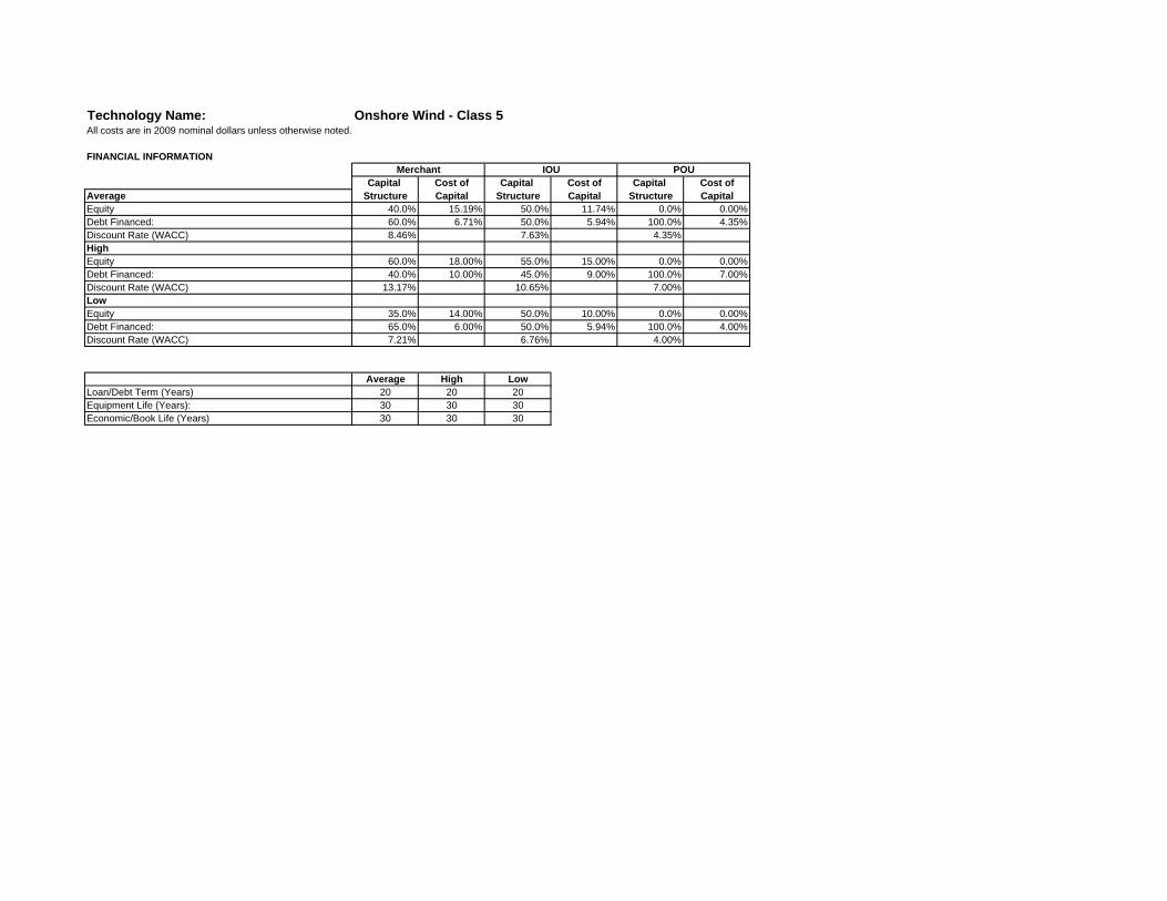
Technology Name: Onshore Wind - Class 5All costs are in 2009 nominal dollars unless otherwise noted.
FINANCIAL INFORMATION
Capital Cost of Capital Cost of Capital Cost ofAverage Structure Capital Structure Capital Structure CapitalEquity 40.0% 15.19% 50.0% 11.74% 0.0% 0.00%Debt Financed: 60.0% 6.71% 50.0% 5.94% 100.0% 4.35%Discount Rate (WACC) 8.46% 7.63% 4.35%HighEquity 60.0% 18.00% 55.0% 15.00% 0.0% 0.00%Debt Financed: 40.0% 10.00% 45.0% 9.00% 100.0% 7.00%Discount Rate (WACC) 13.17% 10.65% 7.00%LowEquity 35.0% 14.00% 50.0% 10.00% 0.0% 0.00%Debt Financed: 65.0% 6.00% 50.0% 5.94% 100.0% 4.00%Discount Rate (WACC) 7.21% 6.76% 4.00%
Average High LowLoan/Debt Term (Years) 20 20 20Equipment Life (Years): 30 30 30Economic/Book Life (Years) 30 30 30
Merchant IOU POU

Technology Name: Onshore Wind - Class 5All costs are in 2009 nominal dollars unless otherwise noted.
TAX INFORMATION/BENEFITSFederal Tax 35.00%CA State Tax 8.84%Total Tax Rate 40.7%CA Avg. Ad Valorem Tax 1.07%CA Sales Tax 7.00%
Average High LowFederal Tax Life (Years) 5 5 5State Tax Life (Years) 30 30 30
Renewable Tax Benefits Merchant IOU POU Merchant IOU POU Merchant IOU POUEligible For BETC N N N N N N N N NEligible For Geothermal Depletion Allowance N N N N N N N N NEligible For REPTC Y Y N Y Y N Y Y NEligible For REPI Y Y Y Y Y Y Y Y Y
Business Energy Tax Credit (BETC) BETC Limit ($) $25,000 $25,000 $25,000 $25,000 $25,000 $25,000 $25,000 $25,000 $25,000 BETC Limit (% Of Remaining Taxes) 25% 25% 25% 25% 25% 25% 25% 25% 25% BETC Calculation $0 $0 $0 $0 $0 $0 $0 $0 $0Geothermal Depletion Allowance Percentage Depletion 15% 15% 15% 15% 15% 15% 15% 15% 15% Limit (% Of Remaining Taxes) 50% 50% 50% 50% 50% 50% 50% 50% 50% Amount ($/kWh) 0.019 0.019 0.019 0.019 0.019 0.019 0.019 0.019 0.019Renewable Energy Production Tax Credit (REPTC) Duration (Years) 10 10 10 10 10 10 10 10 10 REPTC Base Year 2005 2005 2005 2005 2005 2005 2005 2005 2005 REPTC In Start Year 0.019 0.019 0.019 0.019 0.019 0.019 0.019 0.019 0.019
REPI Tier REPI Tier Proportion Paid Tier 1 Tier 1 Tier 1 Tier 1 Tier 1 Tier 1 Tier 1 Tier 1 Tier 1 REPI Duration 10 10 10 10 10 10 10 10 10 REPI Base Year 2009 2009 2009 2009 2009 2009 2009 2009 2009 REPI In Start Year ($/kWh) 0.021 0.021 0.021 0.021 0.021 0.021 0.021 0.021 0.021
LowAverage High

Technology Name: Onshore Wind - Class 3/4All costs are in 2009 nominal dollars unless otherwise noted.
Year=2009, Value & DollarsPLANT DATA Average High LowGross Capacity (MW) 50 30 100Station Service (%) 0.10% 0.10% 0.10%Net Capacity (MW) 49.95 29.97 99.90Net Energy (GWh) 162 108 298Transformer Losses 0.50% 0.50% 0.50%Tranmission losses 5.00% 5.00% 5.00%Load Center Delivered Capacity (MW) 47.22 28.33 94.43Net Capacity Factor (NCF) 37% 41% 34%Planned Percent of Year Operational 100.0% 100.0% 100.0%Average Percent Output 38.29% 42.92% 34.78%Net Energy Delivered to Load Center (GWh) 153 102 281Forced Outage Rate (FOR) 2.0% 2.7% 1.3%Scheduled Outage Factor (SOF) 1.39% 1.83% 0.96%Curtailment (Hours) 0.0 0.0 0.0Degradation Factors Capacity Degradation (%/Year) 1.00% 1.00% 1.00% Heat Rate Degradation (%/Year) 0 0 0Emission Factors NOX (lbs/MWh) 0 0 0 VOC/ROG (Lbs/MWh) 0 0 0 CO (Lbs/MWh) 0 0 0 CO2 (lbs/MWh) 0 0 0 SOX (lbs/MWh) 0 0 0 PM10 (lbs/MWh) 0 0 0

Technology Name: Onshore Wind - Class 3/4All costs are in 2009 nominal dollars unless otherwise noted.
Start Year 2009 2010 2011 2012 2013 2014 2015 2016 2017 2018 2019PLANT COST DATA Average 1 0.99855948 0.99855948 0.992858959 0.992858959 0.992858959 0.992426353 0.98644194 0.98644194 0.98644194 0.986325258 Instant Cost (Nominal $/Gross MW) $1,990,000 $2,042,773 $2,099,971 $2,146,446 $2,206,547 $2,268,330 $2,330,827 $2,381,642 $2,448,328 $2,516,881 $2,587,047 Installed Cost (Nominal $/Gross MW) $2,331,817 $2,393,655 $2,460,677 $2,515,136 $2,585,559 $2,657,955 $2,731,187 $2,790,730 $2,868,871 $2,949,199 $3,031,418 % Cost first year of construction 5% 5% 5% 5% 5% 5% 5% 5% 5% 5% 5% % Cost second year of construction 95% 95% 95% 95% 95% 95% 95% 95% 95% 95% 95% % Cost third year of construction High 1 0.999680986 0.999680986 0.998415036 0.998415036 0.998415036 0.998318733 0.996983179 0.996983179 0.996983179 0.996957076 Instant Cost (Nominal $/Gross MW) $3,025,000 $3,108,708 $3,195,752 $3,281,073 $3,372,943 $3,467,385 $3,564,128 $3,659,022 $3,761,475 $3,866,796 $3,974,962 Installed Cost (Nominal $/Gross MW) $3,784,917 $3,889,653 $3,998,564 $4,105,318 $4,220,267 $4,338,434 $4,459,480 $4,578,213 $4,706,403 $4,838,182 $4,973,521 % Cost first year of construction 2% 2% 2% 2% 2% 2% 2% 2% 2% 2% 2% % Cost second year of construction 45% 45% 45% 45% 45% 45% 45% 45% 45% 45% 45% % Cost third year of construction 45% 45% 45% 45% 45% 45% 45% 45% 45% 45% 45% Low 1 0.997952035 0.997952035 0.98985993 0.98985993 0.98985993 0.989246628 0.980774168 0.980774168 0.980774168 0.98060919 Instant Cost (Nominal $/Gross MW) $1,440,000 $1,477,288 $1,518,652 $1,548,516 $1,591,874 $1,636,446 $1,681,225 $1,713,497 $1,761,475 $1,810,796 $1,861,185 Installed Cost (Nominal $/Gross MW) $1,644,029 $1,686,601 $1,733,826 $1,767,920 $1,817,422 $1,868,310 $1,919,432 $1,956,277 $2,011,053 $2,067,362 $2,124,891 % Cost first year of construction 10% 10% 10% 10% 10% 10% 10% 10% 10% 10% 10% % Cost second year of construction 90% 90% 90% 90% 90% 90% 90% 90% 90% 90% 90% % Cost third year of construction
Start Year 2020 2021 2022 2023 2024 2025 2026 2027 2028 2029PLANT COST DATA Average 0.981196149 0.974971867 0.971135258 0.96493117 0.962109094 0.956894598 0.950522181 0.949490099 0.942596731 0.940398379 Instant Cost (Nominal $/Gross MW) $2,614,772 $2,639,756 $2,671,438 $2,696,841 $2,731,977 $2,760,645 $2,786,137 $2,827,641 $2,852,026 $2,890,901 Installed Cost (Nominal $/Gross MW) $3,063,904 $3,093,180 $3,130,304 $3,160,071 $3,201,242 $3,234,834 $3,264,704 $3,313,338 $3,341,912 $3,387,463 % Cost first year of construction 5% 5% 5% 5% 5% 5% 5% 5% 5% 5% % Cost second year of construction 95% 95% 95% 95% 95% 95% 95% 95% 95% 95% % Cost third year of construction High 0.995807266 0.994405643 0.993538217 0.99212986 0.991486901 0.990294999 0.98883154 0.988593799 0.98700072 0.986490767 Instant Cost (Nominal $/Gross MW) $4,033,904 $4,092,677 $4,154,533 $4,215,022 $4,279,687 $4,342,935 $4,405,902 $4,475,320 $4,539,598 $4,609,848 Installed Cost (Nominal $/Gross MW) $5,047,269 $5,120,808 $5,198,202 $5,273,887 $5,354,797 $5,433,934 $5,512,718 $5,599,575 $5,680,000 $5,767,898 % Cost first year of construction 2% 2% 2% 2% 2% 2% 2% 2% 2% 2% % Cost second year of construction 45% 45% 45% 45% 45% 45% 45% 45% 45% 45% % Cost third year of construction 45% 45% 45% 45% 45% 45% 45% 45% 45% 45% Low 0.973365236 0.964595993 0.959202437 0.950499672 0.946548815 0.939261478 0.930378667 0.92894236 0.919366048 0.916318284 Instant Cost (Nominal $/Gross MW) $1,876,995 $1,889,846 $1,909,348 $1,922,297 $1,944,935 $1,960,841 $1,973,374 $2,001,852 $2,012,915 $2,038,342 Installed Cost (Nominal $/Gross MW) $2,142,941 $2,157,613 $2,179,877 $2,194,661 $2,220,507 $2,238,667 $2,252,975 $2,285,489 $2,298,119 $2,327,149 % Cost first year of construction 10% 10% 10% 10% 10% 10% 10% 10% 10% 10% % Cost second year of construction 90% 90% 90% 90% 90% 90% 90% 90% 90% 90% % Cost third year of construction

Technology Name: Onshore Wind - Class 3/4All costs are in 2009 nominal dollars unless otherwise noted.
Average High LowFixed Cost ($/kW-Year) $13.70 $17.13 $10.28Variable Cost ($/MWh) $5.50 $7.66 $4.82
Start Year 2009 2010 2011 2012 2013 2014 2015 2016 2017 2018 2019FUEL COST DATAFuel Use N/A N/A N/A N/A N/A N/A N/A N/A N/A N/A N/AFuel Cost $/mmBtu) Average N/A N/A N/A N/A N/A N/A N/A N/A N/A N/A N/A High N/A N/A N/A N/A N/A N/A N/A N/A N/A N/A N/A Low N/A N/A N/A N/A N/A N/A N/A N/A N/A N/A N/AHeat Rate (Btu/kWh) Average N/A N/A N/A N/A N/A N/A N/A N/A N/A N/A N/A High N/A N/A N/A N/A N/A N/A N/A N/A N/A N/A N/A Low N/A N/A N/A N/A N/A N/A N/A N/A N/A N/A N/A
Start Year 2020 2021 2022 2023 2024 2025 2026 2027 2028 2029FUEL COST DATAFuel Use N/A N/A N/A N/A N/A N/A N/A N/A N/A N/AFuel Cost $/mmBtu) Average N/A N/A N/A N/A N/A N/A N/A N/A N/A N/A High N/A N/A N/A N/A N/A N/A N/A N/A N/A N/A Low N/A N/A N/A N/A N/A N/A N/A N/A N/A N/AHeat Rate (Btu/kWh) Average N/A N/A N/A N/A N/A N/A N/A N/A N/A N/A High N/A N/A N/A N/A N/A N/A N/A N/A N/A N/A Low N/A N/A N/A N/A N/A N/A N/A N/A N/A N/A

Technology Name: Onshore Wind - Class 3/4All costs are in 2009 nominal dollars unless otherwise noted.
FINANCIAL INFORMATION
Capital Cost of Capital Cost of Capital Cost ofAverage Structure Capital Structure Capital Structure CapitalEquity 40.0% 15.19% 50.0% 11.74% 0.0% 0.00%Debt Financed: 60.0% 6.71% 50.0% 5.94% 100.0% 4.35%Discount Rate (WACC) 8.46% 7.63% 4.35%HighEquity 60.0% 18.00% 55.0% 15.00% 0.0% 0.00%Debt Financed: 40.0% 10.00% 45.0% 9.00% 100.0% 7.00%Discount Rate (WACC) 13.17% 10.65% 7.00%LowEquity 35.0% 14.00% 50.0% 10.00% 0.0% 0.00%Debt Financed: 65.0% 6.00% 50.0% 5.94% 100.0% 4.00%Discount Rate (WACC) 7.21% 6.76% 4.00%
Average High LowLoan/Debt Term (Years) 20 20 20Equipment Life (Years): 30 30 30Economic/Book Life (Years) 30 30 30
Merchant IOU POU

Technology Name: Onshore Wind - Class 3/4All costs are in 2009 nominal dollars unless otherwise noted.
TAX INFORMATION/BENEFITSFederal Tax 35.00%CA State Tax 8.84%Total Tax Rate 40.7%CA Avg. Ad Valorem Tax 1.07%CA Sales Tax 7.00%
Average High LowFederal Tax Life (Years) 5 5 5State Tax Life (Years) 30 30 30
Renewable Tax Benefits Merchant IOU POU Merchant IOU POU Merchant IOU POUEligible For BETC N N N N N N N N NEligible For Geothermal Depletion Allowance N N N N N N N N NEligible For REPTC Y Y N Y Y N Y Y NEligible For REPI Y Y Y Y Y Y Y Y Y
Business Energy Tax Credit (BETC) BETC Limit ($) $25,000 $25,000 $25,000 $25,000 $25,000 $25,000 $25,000 $25,000 $25,000 BETC Limit (% Of Remaining Taxes) 25% 25% 25% 25% 25% 25% 25% 25% 25% BETC Calculation $0 $0 $0 $0 $0 $0 $0 $0 $0Geothermal Depletion Allowance Percentage Depletion 15% 15% 15% 15% 15% 15% 15% 15% 15% Limit (% Of Remaining Taxes) 50% 50% 50% 50% 50% 50% 50% 50% 50% Amount ($/kWh) 0.021 0.021 0.021 0.021 0.021 0.021 0.021 0.021 0.021Renewable Energy Production Tax Credit (REPTC) Duration (Years) 10 10 10 10 10 10 10 10 10 REPTC Base Year 2009 2009 2009 2009 2009 2009 2009 2009 2009 REPTC In Start Year 0.021 0.021 0.021 0.021 0.021 0.021 0.021 0.021 0.021
REPI Tier REPI Tier Proportion Paid Tier 1 Tier 1 Tier 1 Tier 1 Tier 1 Tier 1 Tier 1 Tier 1 Tier 1 REPI Duration 10 10 10 10 10 10 10 10 10 REPI Base Year 2009 2009 2009 2009 2009 2009 2009 2009 2009 REPI In Start Year ($/kWh) 0.021 0.021 0.021 0.021 0.021 0.021 0.021 0.021 0.021
LowAverage High

Technology Name: Offshore Wind - Class 5All costs are in 2009 nominal dollars unless otherwise noted.
Year=2009, Value & DollarsPLANT DATA Average High LowGross Capacity (MW) 100 50 350Station Service (%) 0.10% 0.10% 0.10%Net Capacity (MW) 99.90 49.95 349.65Net Energy (GWh) 394 184 1470Transformer Losses 0.50% 0.50% 0.50%Tranmission losses 5.00% 5.00% 5.00%Load Center Delivered Capacity (MW) 94.43 47.22 330.51Net Capacity Factor (NCF) 45% 42% 48%Planned Percent of Year Operational 100.0% 100.0% 100.0%Average Percent Output 47.15% 44.63% 49.60%Net Energy Delivered to Load Center (GWh) 372 174 1390Forced Outage Rate (FOR) 2.0% 2.7% 1.3%Scheduled Outage Factor (SOF) 2.62% 3.29% 1.96%Curtailment (Hours) 0.0 0.0 0.0Degradation Factors Capacity Degradation (%/Year) 1.00% 1.00% 1.00% Heat Rate Degradation (%/Year) 0 0 0Emission Factors NOX (lbs/MWh) 0 0 0 VOC/ROG (Lbs/MWh) 0 0 0 CO (Lbs/MWh) 0 0 0 CO2 (lbs/MWh) 0 0 0 SOX (lbs/MWh) 0 0 0 PM10 (lbs/MWh) 0 0 0

Technology Name: Offshore Wind - Class 5All costs are in 2009 nominal dollars unless otherwise noted.
Start Year 2009 2010 2011 2012 2013 2014 2015 2016 2017 2018 2019PLANT COST DATA Average 1 0.931857019 0.891021848 0.85855458 0.826608704 0.798099338 0.772699122 0.748455365 0.72529479 0.70181175 0.67858922 Instant Cost (Nominal $/Gross MW) $5,587,937 $5,284,651 $5,134,323 $5,022,499 $4,912,766 $4,816,651 $4,737,886 $4,663,611 $4,592,277 $4,515,023 $4,435,474 Installed Cost (Nominal $/Gross MW) $6,547,763 $6,192,382 $6,016,232 $5,885,201 $5,756,620 $5,643,994 $5,551,701 $5,464,668 $5,381,081 $5,290,557 $5,197,344 % Cost first year of construction 5% 5% 5% 5% 5% 5% 5% 5% 5% 5% 5% % Cost second year of construction 95% 95% 95% 95% 95% 95% 95% 95% 95% 95% 95% % Cost third year of construction High 1.00000 0.97506 0.95955 0.94689 0.93413 0.92247 0.91186 0.90151 0.89143 0.88099 0.87045 Instant Cost (Nominal $/Gross MW) $5,587,937 $5,529,669 $5,529,209 $5,539,259 $5,551,790 $5,567,248 $5,591,138 $5,617,310 $5,644,175 $5,667,760 $5,689,522 Installed Cost (Nominal $/Gross MW) $6,991,695 $6,918,789 $6,918,214 $6,930,788 $6,946,467 $6,965,809 $6,995,700 $7,028,447 $7,062,061 $7,091,570 $7,118,800 % Cost first year of construction 2% 2% 2% 2% 2% 2% 2% 2% 2% 2% 2% % Cost second year of construction 45% 45% 45% 45% 45% 45% 45% 45% 45% 45% 45% % Cost third year of construction 45% 45% 45% 45% 45% 45% 45% 45% 45% 45% 45% Low 1 0.920587662 0.873472411 0.836275958 0.799912775 0.767664996 0.739100692 0.711987429 0.686226537 0.660251412 0.634711382 Instant Cost (Nominal $/Gross MW) $5,587,937 $5,220,742 $5,033,198 $4,892,170 $4,754,105 $4,632,975 $4,531,874 $4,436,380 $4,344,912 $4,247,649 $4,148,674 Installed Cost (Nominal $/Gross MW) $6,379,675 $5,960,453 $5,746,336 $5,585,327 $5,427,700 $5,289,407 $5,173,981 $5,064,958 $4,960,530 $4,849,486 $4,736,487 % Cost first year of construction 10% 10% 10% 10% 10% 10% 10% 10% 10% 10% 10% % Cost second year of construction 90% 90% 90% 90% 90% 90% 90% 90% 90% 90% 90% % Cost third year of construction
Start Year 2020 2021 2022 2023 2024 2025 2026 2027 2028 2029PLANT COST DATA Average 0.656668505 0.638029178 0.62220396 0.608458307 0.596311246 0.585431062 0.575684613 0.56685994 0.558799059 0.551381156 Instant Cost (Nominal $/Gross MW) $4,360,868 $4,304,879 $4,265,274 $4,237,783 $4,219,632 $4,208,924 $4,205,074 $4,206,864 $4,213,394 $4,223,982 Installed Cost (Nominal $/Gross MW) $5,109,923 $5,044,318 $4,997,909 $4,965,696 $4,944,427 $4,931,880 $4,927,369 $4,929,466 $4,937,118 $4,949,524 % Cost first year of construction 5% 5% 5% 5% 5% 5% 5% 5% 5% 5% % Cost second year of construction 95% 95% 95% 95% 95% 95% 95% 95% 95% 95% % Cost third year of construction High 0.86028 0.85146 0.84384 0.83712 0.83111 0.82565 0.82070 0.81618 0.81201 0.80813 Instant Cost (Nominal $/Gross MW) $5,713,030 $5,744,936 $5,784,632 $5,830,392 $5,881,086 $5,935,941 $5,994,794 $6,057,135 $6,122,590 $6,190,876 Installed Cost (Nominal $/Gross MW) $7,148,213 $7,188,134 $7,237,802 $7,295,057 $7,358,487 $7,427,121 $7,500,759 $7,578,761 $7,660,659 $7,746,100 % Cost first year of construction 2% 2% 2% 2% 2% 2% 2% 2% 2% 2% % Cost second year of construction 45% 45% 45% 45% 45% 45% 45% 45% 45% 45% % Cost third year of construction 45% 45% 45% 45% 45% 45% 45% 45% 45% 45% Low 0.610740874 0.590466668 0.573333261 0.558512108 0.545462544 0.533812803 0.523408613 0.514014553 0.505455562 0.497598059 Instant Cost (Nominal $/Gross MW) $4,055,867 $3,983,968 $3,930,260 $3,889,918 $3,859,815 $3,837,817 $3,823,225 $3,814,680 $3,811,179 $3,811,964 Installed Cost (Nominal $/Gross MW) $4,630,531 $4,548,444 $4,487,127 $4,441,069 $4,406,701 $4,381,586 $4,364,926 $4,355,170 $4,351,174 $4,352,070 % Cost first year of construction 10% 10% 10% 10% 10% 10% 10% 10% 10% 10% % Cost second year of construction 90% 90% 90% 90% 90% 90% 90% 90% 90% 90% % Cost third year of construction
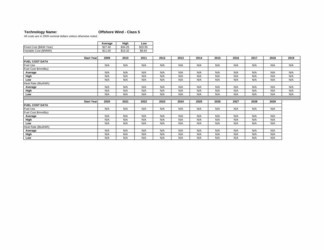
Technology Name: Offshore Wind - Class 5All costs are in 2009 nominal dollars unless otherwise noted.
Average High LowFixed Cost ($/kW-Year) $27.40 $34.25 $20.55Variable Cost ($/MWh) $11.00 $15.32 $9.64
Start Year 2009 2010 2011 2012 2013 2014 2015 2016 2017 2018 2019FUEL COST DATAFuel Use N/A N/A N/A N/A N/A N/A N/A N/A N/A N/A N/AFuel Cost $/mmBtu) Average N/A N/A N/A N/A N/A N/A N/A N/A N/A N/A N/A High N/A N/A N/A N/A N/A N/A N/A N/A N/A N/A N/A Low N/A N/A N/A N/A N/A N/A N/A N/A N/A N/A N/AHeat Rate (Btu/kWh) Average N/A N/A N/A N/A N/A N/A N/A N/A N/A N/A N/A High N/A N/A N/A N/A N/A N/A N/A N/A N/A N/A N/A Low N/A N/A N/A N/A N/A N/A N/A N/A N/A N/A N/A
Start Year 2020 2021 2022 2023 2024 2025 2026 2027 2028 2029FUEL COST DATAFuel Use N/A N/A N/A N/A N/A N/A N/A N/A N/A N/AFuel Cost $/mmBtu) Average N/A N/A N/A N/A N/A N/A N/A N/A N/A N/A High N/A N/A N/A N/A N/A N/A N/A N/A N/A N/A Low N/A N/A N/A N/A N/A N/A N/A N/A N/A N/AHeat Rate (Btu/kWh) Average N/A N/A N/A N/A N/A N/A N/A N/A N/A N/A High N/A N/A N/A N/A N/A N/A N/A N/A N/A N/A Low N/A N/A N/A N/A N/A N/A N/A N/A N/A N/A

Technology Name: Offshore Wind - Class 5All costs are in 2009 nominal dollars unless otherwise noted.
FINANCIAL INFORMATION
Capital Cost of Capital Cost of Capital Cost ofAverage Structure Capital Structure Capital Structure CapitalEquity 40.0% 15.19% 50.0% 11.74% 0.0% 0.00%Debt Financed: 60.0% 6.71% 50.0% 5.94% 100.0% 4.35%Discount Rate (WACC) 8.46% 7.63% 4.35%HighEquity 60.0% 18.00% 55.0% 15.00% 0.0% 0.00%Debt Financed: 40.0% 10.00% 45.0% 9.00% 100.0% 7.00%Discount Rate (WACC) 13.17% 10.65% 7.00%LowEquity 35.0% 14.00% 50.0% 10.00% 0.0% 0.00%Debt Financed: 65.0% 6.00% 50.0% 5.94% 100.0% 4.00%Discount Rate (WACC) 7.21% 6.76% 4.00%
Average High LowLoan/Debt Term (Years) 20 20 20Equipment Life (Years): 30 30 30Economic/Book Life (Years) 30 30 30
Merchant IOU POU

Technology Name: Offshore Wind - Class 5All costs are in 2009 nominal dollars unless otherwise noted.
TAX INFORMATION/BENEFITSFederal Tax 35.00%CA State Tax 8.84%Total Tax Rate 40.7%CA Avg. Ad Valorem Tax 1.07%CA Sales Tax 7.00%
Average High LowFederal Tax Life (Years) 5 5 5State Tax Life (Years) 30 30 30
Renewable Tax Benefits Merchant IOU POU Merchant IOU POU Merchant IOU POUEligible For BETC N N N N N N N N NEligible For Geothermal Depletion Allowance N N N N N N N N NEligible For REPTC Y Y N Y Y N Y Y NEligible For REPI Y Y Y Y Y Y Y Y Y
Business Energy Tax Credit (BETC) BETC Limit ($) $25,000 $25,000 $25,000 $25,000 $25,000 $25,000 $25,000 $25,000 $25,000 BETC Limit (% Of Remaining Taxes) 25% 25% 25% 25% 25% 25% 25% 25% 25% BETC Calculation $0 $0 $0 $0 $0 $0 $0 $0 $0Geothermal Depletion Allowance Percentage Depletion 15% 15% 15% 15% 15% 15% 15% 15% 15% Limit (% Of Remaining Taxes) 50% 50% 50% 50% 50% 50% 50% 50% 50% Amount ($/kWh) 0.019 0.019 0.019 0.019 0.019 0.019 0.019 0.019 0.019Renewable Energy Production Tax Credit (REPTC) Duration (Years) 10 10 10 10 10 10 10 10 10 REPTC Base Year 2009 2009 2009 2009 2009 2009 2009 2009 2009 REPTC In Start Year 0.021 0.021 0.021 0.021 0.021 0.021 0.021 0.021 0.021
REPI Tier REPI Tier Proportion Paid Tier 1 Tier 1 Tier 1 Tier 1 Tier 1 Tier 1 Tier 1 Tier 1 Tier 1 REPI Duration 10 10 10 10 10 10 10 10 10 REPI Base Year 2006 2006 2006 2006 2006 2006 2006 2006 2006 REPI In Start Year ($/kWh) 0.000 0.000 0.000 0.000 0.000 0.000 0.000 0.000 0.000
LowAverage High

Technology Name: Ocean WaveAll costs are in 2009 nominal dollars unless otherwise noted.
Year=2009, Value & DollarsPLANT DATA Average High LowGross Capacity (MW) 40 5 100Station Service (%) 1.00% 1.00% 1.00%Net Capacity (MW) 39.60 4.95 99.00Net Energy (GWh) 90 9 260Transformer Losses 0.50% 0.50% 0.50%Tranmission losses 5.00% 5.00% 5.00%Load Center Delivered Capacity (MW) 37.43 4.68 93.58Net Capacity Factor (NCF) 26.00% 21.00% 30.00%Planned Percent of Year Operational 100.0% 100.0% 100.0%Average Percent Output 30.24% 24.87% 34.34%Net Energy Delivered to Load Center (GWh) 85 9 246Forced Outage Rate (FOR) 5.1% 6.7% 3.8%Scheduled Outage Factor (SOF) 9.40% 9.56% 9.20%Curtailment (Hours) 0.0 0.0 0.0Degradation Factors Capacity Degradation (%/Year) 1.00% 1.00% 1.00% Heat Rate Degradation (%/Year) 0 0 0Emission Factors NOX (lbs/MWh) 0 0 0 VOC/ROG (Lbs/MWh) 0 0 0 CO (Lbs/MWh) 0 0 0 CO2 (lbs/MWh) 0 0 0 SOX (lbs/MWh) 0 0 0 PM10 (lbs/MWh) 0 0 0

Technology Name: Ocean WaveAll costs are in 2009 nominal dollars unless otherwise noted.
Start Year 2009 2010 2011 2012 2013 2014 2015 2016 2017 2018 2019PLANT COST DATA Average Instant Cost (Nominal $/Gross MW) $2,586,645 $2,625,140 $2,667,351 $2,707,929 $2,751,132 $2,793,660 $2,838,308 $2,884,309 $2,930,886 $2,978,000 $3,029,989 Installed Cost (Nominal $/Gross MW) $2,696,059 $2,736,182 $2,780,179 $2,822,473 $2,867,504 $2,911,831 $2,958,367 $3,006,314 $3,054,861 $3,103,968 $3,158,157 % Cost first year of construction 100% 100% 100% 100% 100% 100% 100% 100% 100% 100% 100% % Cost second year of construction % Cost third year of construction High Instant Cost (Nominal $/Gross MW) $2,854,169 $2,896,645 $2,943,222 $2,987,997 $3,035,669 $3,082,595 $3,131,861 $3,182,619 $3,234,013 $3,286,000 $3,029,989 Installed Cost (Nominal $/Gross MW) $3,485,311 $3,537,179 $3,594,056 $3,648,732 $3,706,945 $3,764,248 $3,824,408 $3,886,391 $3,949,149 $4,012,632 $3,700,010 % Cost first year of construction 40% 40% 40% 40% 40% 40% 40% 40% 40% 40% 40% % Cost second year of construction 60% 60% 60% 60% 60% 60% 60% 60% 60% 60% 60% % Cost third year of construction Low Instant Cost (Nominal $/Gross MW) $2,365,156 $2,400,354 $2,438,951 $2,476,055 $2,515,559 $2,554,445 $2,595,270 $2,637,332 $2,679,920 $2,723,000 $3,029,989 Installed Cost (Nominal $/Gross MW) $2,450,431 $2,486,898 $2,526,886 $2,565,328 $2,606,256 $2,646,544 $2,688,841 $2,732,419 $2,776,543 $2,821,176 $3,139,234 % Cost first year of construction 100% 100% 100% 100% 100% 100% 100% 100% 100% 100% 100% % Cost second year of construction % Cost third year of construction
Start Year 2020 2021 2022 2023 2024 2025 2026 2027 2028 2029PLANT COST DATA Average Instant Cost (Nominal $/Gross MW) $3,081,979 $3,133,968 $3,185,958 $3,237,947 $3,289,936 $3,341,926 $3,393,915 $3,445,904 $3,497,894 $3,549,883 Installed Cost (Nominal $/Gross MW) $3,212,345 $3,266,534 $3,320,722 $3,374,911 $3,429,099 $3,483,288 $3,537,476 $3,591,665 $3,645,853 $3,700,042 % Cost first year of construction 100% 100% 100% 100% 100% 100% 100% 100% 100% 100% % Cost second year of construction % Cost third year of construction High Instant Cost (Nominal $/Gross MW) $3,081,979 $3,133,968 $3,185,958 $3,237,947 $3,289,936 $3,341,926 $3,393,915 $3,445,904 $3,497,894 $3,549,883 Installed Cost (Nominal $/Gross MW) $3,763,496 $3,826,982 $3,890,468 $3,953,953 $4,017,439 $4,080,925 $4,144,411 $4,207,896 $4,271,382 $4,334,868 % Cost first year of construction 40% 40% 40% 40% 40% 40% 40% 40% 40% 40% % Cost second year of construction 60% 60% 60% 60% 60% 60% 60% 60% 60% 60% % Cost third year of construction Low Instant Cost (Nominal $/Gross MW) $3,081,979 $3,133,968 $3,185,958 $3,237,947 $3,289,936 $3,341,926 $3,393,915 $3,445,904 $3,497,894 $3,549,883 Installed Cost (Nominal $/Gross MW) $3,193,098 $3,246,962 $3,300,826 $3,354,690 $3,408,553 $3,462,417 $3,516,281 $3,570,145 $3,624,009 $3,677,873 % Cost first year of construction 100% 100% 100% 100% 100% 100% 100% 100% 100% 100% % Cost second year of construction % Cost third year of construction

Technology Name: Ocean WaveAll costs are in 2009 nominal dollars unless otherwise noted.
Average High LowFixed Cost ($/kW-Year) $36.00 $43.00 $27.00Variable Cost ($/MWh) $12.00 $14.00 $9.00
Start Year 2009 2010 2011 2012 2013 2014 2015 2016 2017 2018 2019FUEL COST DATAFuel Use N/A N/A N/A N/A N/A N/A N/A N/A N/A N/A N/AFuel Cost $/mmBtu) Average N/A N/A N/A N/A N/A N/A N/A N/A N/A N/A N/A High N/A N/A N/A N/A N/A N/A N/A N/A N/A N/A N/A Low N/A N/A N/A N/A N/A N/A N/A N/A N/A N/A N/AHeat Rate (Btu/kWh) Average N/A N/A N/A N/A N/A N/A N/A N/A N/A N/A N/A High N/A N/A N/A N/A N/A N/A N/A N/A N/A N/A N/A Low N/A N/A N/A N/A N/A N/A N/A N/A N/A N/A N/A
Start Year 2020 2021 2022 2023 2024 2025 2026 2027 2028 2029FUEL COST DATAFuel Use N/A N/A N/A N/A N/A N/A N/A N/A N/A N/AFuel Cost $/mmBtu) Average N/A N/A N/A N/A N/A N/A N/A N/A N/A N/A High N/A N/A N/A N/A N/A N/A N/A N/A N/A N/A Low N/A N/A N/A N/A N/A N/A N/A N/A N/A N/AHeat Rate (Btu/kWh) Average N/A N/A N/A N/A N/A N/A N/A N/A N/A N/A High N/A N/A N/A N/A N/A N/A N/A N/A N/A N/A Low N/A N/A N/A N/A N/A N/A N/A N/A N/A N/A

Technology Name: Ocean WaveAll costs are in 2009 nominal dollars unless otherwise noted.
FINANCIAL INFORMATION
Capital Cost of Capital Cost of Capital Cost ofAverage Structure Capital Structure Capital Structure CapitalEquity 40.0% 15.19% 50.0% 11.74% 0.0% 0.00%Debt Financed: 60.0% 6.71% 50.0% 5.94% 100.0% 4.35%Discount Rate (WACC) 8.46% 7.63% 4.35%HighEquity 60.0% 18.00% 55.0% 15.00% 0.0% 0.00%Debt Financed: 40.0% 10.00% 45.0% 9.00% 100.0% 7.00%Discount Rate (WACC) 13.17% 10.65% 7.00%LowEquity 35.0% 14.00% 50.0% 10.00% 0.0% 0.00%Debt Financed: 65.0% 6.00% 50.0% 5.94% 100.0% 4.00%Discount Rate (WACC) 7.21% 6.76% 4.00%
Average High LowLoan/Debt Term (Years) 20 20 20Equipment Life (Years): 30 30 30Economic/Book Life (Years) 30 30 30
Merchant IOU POU

Technology Name: Ocean WaveAll costs are in 2009 nominal dollars unless otherwise noted.
TAX INFORMATION/BENEFITSFederal Tax 35.00%CA State Tax 8.84%Total Tax Rate 40.7%CA Avg. Ad Valorem Tax 1.07%CA Sales Tax 7.00%
Average High LowFederal Tax Life (Years) 5 5 5State Tax Life (Years) 30 30 30
Renewable Tax Benefits Merchant IOU POU Merchant IOU POU Merchant IOU POUEligible For BETC N N N N N N N N NEligible For Geothermal Depletion Allowance N N N N N N N N NEligible For REPTC Y Y N Y Y N Y Y NEligible For REPI N N Y N N Y N N Y
Business Energy Tax Credit (BETC) BETC Limit ($) $25,000 $25,000 $25,000 $25,000 $25,000 $25,000 $25,000 $25,000 $25,000 BETC Limit (% Of Remaining Taxes) 25% 25% 25% 25% 25% 25% 25% 25% 25% BETC Calculation $0 $0 $0 $0 $0 $0 $0 $0 $0Geothermal Depletion Allowance Percentage Depletion 15% 15% 15% 15% 15% 15% 15% 15% 15% Limit (% Of Remaining Taxes) 50% 50% 50% 50% 50% 50% 50% 50% 50% Amount ($/kWh) 0.019 0.019 0.019 0.019 0.019 0.019 0.019 0.019 0.019Renewable Energy Production Tax Credit (REPTC) Duration (Years) 10 10 10 10 10 10 10 10 10 REPTC Base Year 2005 2005 2005 2005 2005 2005 2005 2005 2005 REPTC In Start Year 0.019 0.019 0.019 0.019 0.019 0.019 0.019 0.019 0.019
REPI Tier REPI Tier Proportion Paid Tier 1 Tier 1 Tier 1 Tier 1 Tier 1 Tier 1 Tier 1 Tier 1 Tier 1 REPI Duration 10 10 10 10 10 10 10 10 10 REPI Base Year 2006 2006 2006 2006 2006 2006 2006 2006 2006 REPI In Start Year ($/kWh) 0.000 0.000 0.000 0.000 0.000 0.000 0.000 0.000 0.000
LowAverage High

Technology Name: Coal - IGCCAll costs are in 2009 nominal dollars unless otherwise noted.
Year=2009, Value & DollarsPLANT DATA Average High LowGross Capacity (MW) 300 300 600Station Service (%) 6.00% 7.00% 5.00%Net Capacity (MW) 282.00 279.00 570.00Net Energy (GWh) 1976 1711 4494Transformer Losses 0.50% 0.50% 0.50%Tranmission losses 5.00% 5.00% 5.00%Load Center Delivered Capacity (MW) 266.56 263.72 538.79Net Capacity Factor (NCF) 80.00% 70.00% 90.00%Planned Percent of Year Operational 84.21% 97.65% 99.79%Average Percent Output 100.0% 100.0% 100.0%Net Energy Delivered to Load Center (GWh) 1868.06 1617.16 4247.84Forced Outage Rate (FOR) 5.00% 7.50% 2.50%Scheduled Outage Factor (SOF) 15.00% 22.50% 7.50%Curtailment (Hours) 0 0 0Degradation Factors Capacity Degradation (%/Year) 0.05% 0.10% 0.00% Heat Rate Degradation (%/Year) 0.10% 0.20% 0.10%Emission Factors NOX (lbs/MWh) 0.220 0.314 0.126 VOC/ROG (Lbs/MWh) 0.009 0.009 0.009 CO (Lbs/MWh) 0.079 0.079 0.079 CO2 (lbs/MWh) 1532.000 1631.000 1433.000 SOX (lbs/MWh) 0.063 0.094 0.031 PM10 (lbs/MWh) 0.031 0.031 0.031

Technology Name: Coal - IGCCAll costs are in 2009 nominal dollars unless otherwise noted.
Start Year 2009 2010 2011 2012 2013 2014 2015 2016 2017 2018 2019PLANT COST DATA Average 1 0.996056451 0.992128453 0.988215946 0.984318868 0.980437158 0.976570756 0.972719601 0.968883633 0.965062793 0.96125702 Instant Cost (Nominal $/Gross MW) $2,250,000 $2,283,735 $2,317,976 $2,352,730 $2,388,005 $2,423,809 $2,460,150 $2,497,036 $2,534,475 $2,572,475 $2,611,045 Installed Cost (Nominal $/Gross MW) $2,517,373 $2,565,233 $2,614,003 $2,663,700 $2,714,342 $2,765,946 $2,818,532 $2,872,118 $2,926,722 $2,982,364 $3,039,065 % Cost of last year of construction 80% 80% 80% 80% 80% 80% 80% 80% 80% 80% 80% % Cost next to last year of construction 20% 20% 20% 20% 20% 20% 20% 20% 20% 20% 20% % Cost of previous year of construction High 1 1.00217739 1.004359521 1.006546404 1.008738048 1.010934464 1.013135663 1.015341655 1.01755245 1.019768058 1.021988491 Instant Cost (Nominal $/Gross MW) $2,800,000 $2,859,446 $2,920,154 $2,982,150 $3,045,463 $3,110,121 $3,176,150 $3,243,582 $3,312,445 $3,382,771 $3,454,589 Installed Cost (Nominal $/Gross MW) $3,389,673 $3,454,117 $3,519,786 $3,586,704 $3,654,894 $3,724,380 $3,795,188 $3,867,341 $3,940,866 $4,015,790 $4,092,137 % Cost first year of construction 60% 60% 60% 60% 60% 60% 60% 60% 60% 60% 60% % Cost second year of construction 40% 40% 40% 40% 40% 40% 40% 40% 40% 40% 40% % Cost third year of construction 0% 0% 0% 0% 0% 0% 0% 0% 0% 0% 0% Low 1 0.989942125 0.979985411 0.970128841 0.960371406 0.950712111 0.941149968 0.931683999 0.922313238 0.913036727 0.903853518 Instant Cost (Nominal $/Gross MW) $1,700,000 $1,714,897 $1,729,924 $1,745,083 $1,760,375 $1,775,800 $1,791,361 $1,807,059 $1,822,893 $1,838,867 $1,854,980 Installed Cost (Nominal $/Gross MW) $1,874,918 $1,910,563 $1,946,887 $1,983,901 $2,021,618 $2,060,053 $2,099,218 $2,139,128 $2,179,797 $2,221,239 $2,263,469 % Cost first year of construction 80% 80% 80% 80% 80% 80% 80% 80% 80% 80% 80% % Cost second year of construction 20% % Cost third year of construction
Start Year 2020 2021 2022 2023 2024 2025 2026 2027 2028 2029PLANT COST DATA Average 0.957466256 0.953690441 0.949929516 0.946183422 0.942452101 0.938735495 0.935033545 0.931346194 0.927673385 0.924015059 Instant Cost (Nominal $/Gross MW) $2,650,194 $2,689,929 $2,730,260 $2,771,196 $2,812,745 $2,854,917 $2,897,722 $2,941,169 $2,985,267 $3,030,026 Installed Cost (Nominal $/Gross MW) $3,096,843 $3,155,720 $3,215,716 $3,276,852 $3,339,152 $3,402,635 $3,467,325 $3,533,246 $3,600,419 $3,668,870 % Cost of last year of construction 80% 80% 80% 80% 80% 80% 80% 80% 80% 80% % Cost next to last year of construction 20% 20% 20% 20% 20% 20% 20% 20% 20% 20% % Cost of previous year of construction High 1.024213759 1.026443872 1.028678841 1.030918676 1.033163388 1.035412988 1.037667486 1.039926893 1.042191219 1.044460476 Instant Cost (Nominal $/Gross MW) $3,527,932 $3,602,833 $3,679,323 $3,757,437 $3,837,210 $3,918,677 $4,001,873 $4,086,835 $4,173,601 $4,262,209 Installed Cost (Nominal $/Gross MW) $4,169,936 $4,249,215 $4,330,000 $4,412,321 $4,496,208 $4,581,689 $4,668,795 $4,757,558 $4,848,008 $4,940,178 % Cost first year of construction 60% 60% 60% 60% 60% 60% 60% 60% 60% 60% % Cost second year of construction 40% 40% 40% 40% 40% 40% 40% 40% 40% 40% % Cost third year of construction 0% 0% 0% 0% 0% 0% 0% 0% 0% 0% Low 0.894762672 0.885763261 0.876854365 0.868035074 0.859304486 0.850661709 0.84210586 0.833636065 0.825251458 0.816951182 Instant Cost (Nominal $/Gross MW) $1,871,235 $1,887,632 $1,904,173 $1,920,859 $1,937,691 $1,954,671 $1,971,799 $1,989,077 $2,006,507 $2,024,090 Installed Cost (Nominal $/Gross MW) $2,306,502 $2,350,353 $2,395,037 $2,440,571 $2,486,971 $2,534,253 $2,582,434 $2,631,531 $2,681,561 $2,732,542 % Cost first year of construction 80% 80% 80% 80% 80% 80% 80% 80% 80% 80% % Cost second year of construction % Cost third year of construction

Technology Name: Coal - IGCCAll costs are in 2009 nominal dollars unless otherwise noted.
Average High LowFixed Cost ($/kW-Year) $41.7 $52.00 $31.67Variable Cost ($/MWh) $6.67 $8.33 $5.00
Start Year 2009 2010 2011 2012 2013 2014 2015 2016 2017 2018 2019FUEL COST DATAFuel Use 15,936,192 15,915,168 15,894,144 15,873,120 15,852,096 15,831,072 15,810,048 15,789,024 15,768,000 15,746,976 15,725,952 Fuel Cost $/mmBtu) Average $1.80 $2.10 $2.15 $2.20 $2.24 $2.29 $2.34 $2.39 $2.43 $2.48 $2.52 High $3.13 $3.65 $3.74 $3.82 $3.90 $3.99 $4.07 $4.15 $4.23 $4.31 $4.39 Low $1.31 $1.53 $1.57 $1.60 $1.64 $1.67 $1.71 $1.74 $1.78 $1.81 $1.84Heat Rate (Btu/kWh) Nominal 7580 7570 7560 7550 7540 7530 7520 7510 7500 7490 7480 High 8025 8015 8005 7995 7985 7975 7965 7955 7945 7935 7925 Low 7100 7090 7080 7070 7060 7050 7040 7030 7020 7010 7000
Start Year 2020 2021 2022 2023 2024 2025 2026 2027 2028 2029FUEL COST DATAFuel Use 15,704,928 15,683,904 15,662,880 15,641,856 15,620,832 15,599,808 15,578,784 15,557,760 15,536,736 15,515,712 Fuel Cost $/mmBtu) Average $2.57 $2.61 $2.66 $2.70 $2.75 $2.79 $2.84 $2.90 $2.95 $3.01 High $4.47 $4.55 $4.62 $4.70 $4.78 $4.85 $4.95 $5.04 $5.14 $5.23 Low $1.88 $1.91 $1.94 $1.97 $2.00 $2.04 $2.08 $2.11 $2.16 $2.20Heat Rate (Btu/kWh) Nominal 7470 7460 7450 7440 7430 7420 7410 7400 7390 7380 High 7915 7905 7895 7885 7875 7865 7855 7845 7835 7825 Low 6990 6980 6970 6960 6950 6940 6930 6920 6910 6900

Technology Name: Coal - IGCCAll costs are in 2009 nominal dollars unless otherwise noted.
FINANCIAL INFORMATION
Capital Cost of Capital Cost of Capital Cost ofAverage Structure Capital Structure Capital Structure CapitalEquity 40.0% 15.2% 50.0% 11.7% 0.0% 0.0%Debt Financed: 60.0% 6.7% 50.0% 5.9% 100.0% 4.3%Discount Rate (WACC) 9.7% 8.6% 4.3%HighEquity 60.0% 18.0% 55.0% 15.0% 0.0% 0.0%Debt Financed: 40.0% 10.0% 45.0% 9.0% 100.0% 7.0%Discount Rate (WACC) 14.4% 11.9% 7.0%LowEquity 35.0% 14.0% 50.0% 10.0% 0.0% 0.0%Debt Financed: 65.0% 6.0% 50.0% 5.9% 100.0% 4.0%Discount Rate (WACC) 8.5% 7.7% 4.0%
Average High LowLoan/Debt Term (Years) 15 20 10Equipment Life (Years): 40 40 40Economic/Book Life (Years) 20 20 20
Merchant IOU POU

Technology Name: Coal - IGCCAll costs are in 2009 nominal dollars unless otherwise noted.
TAX INFORMATION/BENEFITSFederal Tax 35.00%CA State Tax 8.84%Total Tax Rate 40.7%CA Avg. Ad Valorem Tax 1.07%CA Sales Tax 7.00%
Average High LowFederal Tax Life (Years) 15 15 15State Tax Life (Years) 20 20 20
Renewable Tax Benefits Merchant IOU POU Merchant IOU POU Merchant IOU POUEligible For BETC N N N N N N N N NEligible For Geothermal Depletion Allowance N N N N N N N N NEligible For REPTC N N N N N N N N NEligible For REPI N N N N N N N N NTDMA Y Y N Y Y N Y Y N
Business Energy Tax Credit (BETC) BETC Limit ($) $25,000 $25,000 $25,000 $25,000 $25,000 $25,000 $25,000 $25,000 $25,000 BETC Limit (% Of Remaining Taxes) 25% 25% 25% 25% 25% 25% 25% 25% 25% BETC Calculation $0 $0 $0 $0 $0 $0 $0 $0 $0Geothermal Depletion Allowance Percentage Depletion 15% 15% 15% 15% 15% 15% 15% 15% 15% Limit (% Of Remaining Taxes) 50% 50% 50% 50% 50% 50% 50% 50% 50% Amount ($/kWh) 0.019 0.019 0.019 0.019 0.019 0.019 0.019 0.019 0.019Renewable Energy Production Tax Credit (REPTC) Duration (Years) 10 10 10 10 10 10 10 10 10 REPTC Base Year 2005 2005 2005 2005 2005 2005 2005 2005 2005 REPTC In Start Year 0.019 0.019 0.019 0.019 0.019 0.019 0.019 0.019 0.019REPI Tier REPI Tier Proportion Paid Tier 1 Tier 1 Tier 1 Tier 1 Tier 1 Tier 1 Tier 1 Tier 1 Tier 1 REPI Duration 10 10 10 10 10 10 10 10 10 REPI Base Year 2006 2006 2006 2006 2006 2006 2006 2006 2006 REPI In Start Year ($/kWh) 0.000 0.000 0.000 0.000 0.000 0.000 0.000 0.000 0.000
Average High Low

Technology Name: Nuclear Reactor - WESTINGHOUSE AP 1000All costs are in 2009 nominal dollars unless otherwise noted.
Year=2009PLANT DATA Average High LowGross Capacity (MW) 960 900 1117Station Service (%) 2.20% 3.00% 1.50%Net Capacity (MW) 938.88 873.00 1100.25Net Energy (GWh) 7081 6202 8906Transformer Losses 0.60% 0.70% 0.50%Tranmission losses 1.70% 2.00% 1.40%Load Center Delivered Capacity (MW) 917.38 849.55 1,079.42Net Capacity Factor (NCF) 86.10% 81.10% 92.40%Planned Percent of Year Operational 88.51% 99.46% 99.82%Average Percent Output 91.0% 95.0% 87.0%Net Energy Delivered to Load Center (GWh) 6919.22 6035.52 8737.06Forced Outage Rate (FOR) 2.72% 2.93% 2.59%Scheduled Outage Factor (SOF) 11.12% 16.00% 4.97%Curtailment (% or Hours) - - - Degradation Factors Capacity Degradation (%/Year) 0.20% 0.20% 0.20% Heat Rate Degradation (%/Year) 0.20% 0.20% 0.20%Emission Factors NOX (lbs/MWh) 0.000 0.000 0.000 VOC/ROG (Lbs/MWh) 0.000 0.000 0.000 CO (Lbs/MWh) 0.000 0.000 0.000 CO2 (lbs/MWh) 0.000 0.000 0.000 SOX (lbs/MWh) 0.000 0.000 0.000 PM10 (lbs/MWh) 0.000 0.000 0.000

Technology Name: Nuclear Reactor - WESTINGHOUSE AP 1000All costs are in 2009 nominal dollars unless otherwise noted.
Start Year 2009 2010 2011 2012 2013 2014 2015 2016 2017 2018 2019PLANT COST DATA THESE ARE START YEAR VALUES. THE COSTS CHANGE EACH YEAR DUE TO CHANGES IN TECHNOLOGY COSTS. Average 1 1 1 1 1 1 1 0.996023857 0.979874265 0.974109281 0.967761131 Capital Cost per KW US $4,000,000 $4,259,528 $4,540,996 $4,837,128 $5,156,157 $5,493,670 $5,856,153 $6,219,046 $6,522,919 $6,913,009 $7,183,374 Installed Cost US$/KW) Projected $6,039,075 $6,430,902 $6,855,854 $7,302,944 $7,784,605 $8,294,172 $8,841,437 $9,389,322 $9,848,099 $10,437,045 $10,845,233 % Year0 (Last Year of Contruction) 2.5% 2.5% 2.5% 2.5% 2.5% 2.5% 2.5% 2.5% 2.5% 2.5% 2.5% % Year1 (Next to Last Year of Contruction) 2.0% 2.0% 2.0% 2.0% 2.0% 2.0% 2.0% 2.0% 2.0% 2.0% 2.0% % Year2 (2 years Before Last Year) 7.0% 7.0% 7.0% 7.0% 7.0% 7.0% 7.0% 7.0% 7.0% 7.0% 7.0% % Year3 (3rd years Before Last Year) 15.5% 15.5% 15.5% 15.5% 15.5% 15.5% 15.5% 15.5% 15.5% 15.5% 15.5% % Year4 (4th Year before Last Year) 22.0% 22.0% 22.0% 22.0% 22.0% 22.0% 22.0% 22.0% 22.0% 22.0% 22.0% % Year5 (5th Year before Last Year) 21.0% 21.0% 21.0% 21.0% 21.0% 21.0% 21.0% 21.0% 21.0% 21.0% 21.0% % Year6 (6th Year before Last Year) 18.0% 18.0% 18.0% 18.0% 18.0% 18.0% 18.0% 18.0% 18.0% 18.0% 18.0% % Year7 (7th Year before Last Year) 10.0% 10.0% 10.0% 10.0% 10.0% 10.0% 10.0% 10.0% 10.0% 10.0% 10.0% % Year8 (8th Year before Last Year) 2.0% 2.0% 2.0% 2.0% 2.0% 2.0% 2.0% 2.0% 2.0% 2.0% 2.0%
High 1 1 1 1 1 1 1 0.996786884 0.983710945 0.979033168 0.973876043 Capital Cost per KW US $5,000,000 $5,424,410 $5,891,341 $6,393,360 $6,942,897 $7,536,225 $8,184,204 $8,861,177 $9,498,296 $10,266,809 $10,886,009 Installed Cost US$/KW) Projected $8,847,984 $9,599,018 $10,425,299 $11,313,669 $12,286,128 $13,336,079 $14,482,740 $15,680,710 $16,808,154 $18,168,111 $19,263,846 % Year0 (Last Year of Contruction) 2.5% 2.5% 2.5% 2.5% 2.5% 2.5% 2.5% 2.5% 2.5% 2.5% 2.5% % Year1 (Next to Last Year of Contruction) 2.0% 2.0% 2.0% 2.0% 2.0% 2.0% 2.0% 2.0% 2.0% 2.0% 2.0% % Year2 (2 years Before Last Year) 7.0% 7.0% 7.0% 7.0% 7.0% 7.0% 7.0% 7.0% 7.0% 7.0% 7.0% % Year3 (3rd years Before Last Year) 15.5% 15.5% 15.5% 15.5% 15.5% 15.5% 15.5% 15.5% 15.5% 15.5% 15.5% % Year4 (4th Year before Last Year) 22.0% 22.0% 22.0% 22.0% 22.0% 22.0% 22.0% 22.0% 22.0% 22.0% 22.0% % Year5 (5th Year before Last Year) 21.0% 21.0% 21.0% 21.0% 21.0% 21.0% 21.0% 21.0% 21.0% 21.0% 21.0% % Year6 (6th Year before Last Year) 18.0% 18.0% 18.0% 18.0% 18.0% 18.0% 18.0% 18.0% 18.0% 18.0% 18.0% % Year7 (7th Year before Last Year) 10.0% 10.0% 10.0% 10.0% 10.0% 10.0% 10.0% 10.0% 10.0% 10.0% 10.0% % Year8 (8th Year before Last Year) 2.0% 2.0% 2.0% 2.0% 2.0% 2.0% 2.0% 2.0% 2.0% 2.0% 2.0%
Low 1 1 1 1 1 1 1 0.995255749 0.976024204 0.969173843 0.961639602 Capital Cost per KW US $3,000,000 $3,134,646 $3,279,089 $3,427,347 $3,584,848 $3,747,809 $3,920,140 $4,081,822 $4,187,677 $4,349,878 $4,384,799 Installed Cost US$/KW) Projected $4,324,384 $4,518,471 $4,726,680 $4,940,388 $5,167,420 $5,402,322 $5,650,731 $5,883,788 $6,036,374 $6,270,181 $6,320,518 % Year0 (Last Year of Contruction) 2.5% 2.5% 2.5% 2.5% 2.5% 2.5% 2.5% 2.5% 2.5% 2.5% 2.5% % Year1 (Next to Last Year of Contruction) 2.0% 2.0% 2.0% 2.0% 2.0% 2.0% 2.0% 2.0% 2.0% 2.0% 2.0% % Year2 (2 years Before Last Year) 7.0% 7.0% 7.0% 7.0% 7.0% 7.0% 7.0% 7.0% 7.0% 7.0% 7.0% % Year3 (3rd years Before Last Year) 15.5% 15.5% 15.5% 15.5% 15.5% 15.5% 15.5% 15.5% 15.5% 15.5% 15.5% % Year4 (4th Year before Last Year) 22.0% 22.0% 22.0% 22.0% 22.0% 22.0% 22.0% 22.0% 22.0% 22.0% 22.0% % Year5 (5th Year before Last Year) 21.0% 21.0% 21.0% 21.0% 21.0% 21.0% 21.0% 21.0% 21.0% 21.0% 21.0% % Year6 (6th Year before Last Year) 18.0% 18.0% 18.0% 18.0% 18.0% 18.0% 18.0% 18.0% 18.0% 18.0% 18.0% % Year7 (7th Year before Last Year) 10.0% 10.0% 10.0% 10.0% 10.0% 10.0% 10.0% 10.0% 10.0% 10.0% 10.0% % Year8 (8th Year before Last Year) 2.0% 2.0% 2.0% 2.0% 2.0% 2.0% 2.0% 2.0% 2.0% 2.0% 2.0%

Technology Name: Nuclear Reactor - WESTINGHOUSE AP 1000All costs are in 2009 nominal dollars unless otherwise noted.
Start Year 2020 2021 2022 2023 2024 2025 2026 2027 2028 2029PLANT COST DATA Average 0.964644349 0.963676037 0.960713192 0.959457743 0.955852449 0.953573079 0.949859107 0.944158759 0.940201511 0.932995402 Capital Cost per KW US $7,488,175 $7,973,430 $8,471,698 $9,016,143 $9,572,496 $10,174,249 $10,796,543 $11,430,101 $12,121,367 $12,809,145 Installed Cost US$/KW) Projected $11,305,412 $12,038,035 $12,790,304 $13,612,290 $14,452,255 $15,360,763 $16,300,283 $17,256,809 $18,300,460 $19,338,847 % Year0 (Last Year of Contruction) 2.5% 2.5% 2.5% 2.5% 2.5% 2.5% 2.5% 2.5% 2.5% 2.5% % Year1 (Next to Last Year of Contruction) 2.0% 2.0% 2.0% 2.0% 2.0% 2.0% 2.0% 2.0% 2.0% 2.0% % Year2 (2 years Before Last Year) 7.0% 7.0% 7.0% 7.0% 7.0% 7.0% 7.0% 7.0% 7.0% 7.0% % Year3 (3rd years Before Last Year) 15.5% 15.5% 15.5% 15.5% 15.5% 15.5% 15.5% 15.5% 15.5% 15.5% % Year4 (4th Year before Last Year) 22.0% 22.0% 22.0% 22.0% 22.0% 22.0% 22.0% 22.0% 22.0% 22.0% % Year5 (5th Year before Last Year) 21.0% 21.0% 21.0% 21.0% 21.0% 21.0% 21.0% 21.0% 21.0% 21.0% % Year6 (6th Year before Last Year) 18.0% 18.0% 18.0% 18.0% 18.0% 18.0% 18.0% 18.0% 18.0% 18.0% % Year7 (7th Year before Last Year) 10.0% 10.0% 10.0% 10.0% 10.0% 10.0% 10.0% 10.0% 10.0% 10.0% % Year8 (8th Year before Last Year) 2.0% 2.0% 2.0% 2.0% 2.0% 2.0% 2.0% 2.0% 2.0% 2.0%
High 0.971341646 0.970553946 0.968142796 0.967120687 0.964184047 0.962326321 0.959297539 0.954644414 0.951410986 0.945516215 Capital Cost per KW US $11,572,110 $12,324,394 $13,102,311 $13,947,854 $14,819,245 $15,758,052 $16,734,420 $17,736,931 $18,824,811 $19,922,390 Installed Cost US$/KW) Projected $20,477,968 $21,809,208 $23,185,807 $24,682,078 $26,224,087 $27,885,398 $29,613,175 $31,387,215 $33,312,323 $35,254,596 % Year0 (Last Year of Contruction) 2.5% 2.5% 2.5% 2.5% 2.5% 2.5% 2.5% 2.5% 2.5% 2.5% % Year1 (Next to Last Year of Contruction) 2.0% 2.0% 2.0% 2.0% 2.0% 2.0% 2.0% 2.0% 2.0% 2.0% % Year2 (2 years Before Last Year) 7.0% 7.0% 7.0% 7.0% 7.0% 7.0% 7.0% 7.0% 7.0% 7.0% % Year3 (3rd years Before Last Year) 15.5% 15.5% 15.5% 15.5% 15.5% 15.5% 15.5% 15.5% 15.5% 15.5% % Year4 (4th Year before Last Year) 22.0% 22.0% 22.0% 22.0% 22.0% 22.0% 22.0% 22.0% 22.0% 22.0% % Year5 (5th Year before Last Year) 21.0% 21.0% 21.0% 21.0% 21.0% 21.0% 21.0% 21.0% 21.0% 21.0% % Year6 (6th Year before Last Year) 18.0% 18.0% 18.0% 18.0% 18.0% 18.0% 18.0% 18.0% 18.0% 18.0% % Year7 (7th Year before Last Year) 10.0% 10.0% 10.0% 10.0% 10.0% 10.0% 10.0% 10.0% 10.0% 10.0% % Year8 (8th Year before Last Year) 2.0% 2.0% 2.0% 2.0% 2.0% 2.0% 2.0% 2.0% 2.0% 2.0%
Low 0.957943976 0.9567963 0.953286026 0.951799247 0.947531733 0.944835296 0.940444434 0.933711637 0.929042276 0.920549195 Capital Cost per KW US $4,436,960 $4,501,987 $4,556,196 $4,620,324 $4,671,872 $4,730,334 $4,780,450 $4,817,767 $4,865,297 $4,892,664 Installed Cost US$/KW) Projected $6,395,706 $6,489,439 $6,567,580 $6,660,018 $6,734,322 $6,818,594 $6,890,833 $6,944,625 $7,013,137 $7,052,585 % Year0 (Last Year of Contruction) 2.5% 2.5% 2.5% 2.5% 2.5% 2.5% 2.5% 2.5% 2.5% 2.5% % Year1 (Next to Last Year of Contruction) 2.0% 2.0% 2.0% 2.0% 2.0% 2.0% 2.0% 2.0% 2.0% 2.0% % Year2 (2 years Before Last Year) 7.0% 7.0% 7.0% 7.0% 7.0% 7.0% 7.0% 7.0% 7.0% 7.0% % Year3 (3rd years Before Last Year) 15.5% 15.5% 15.5% 15.5% 15.5% 15.5% 15.5% 15.5% 15.5% 15.5% % Year4 (4th Year before Last Year) 22.0% 22.0% 22.0% 22.0% 22.0% 22.0% 22.0% 22.0% 22.0% 22.0% % Year5 (5th Year before Last Year) 21.0% 21.0% 21.0% 21.0% 21.0% 21.0% 21.0% 21.0% 21.0% 21.0% % Year6 (6th Year before Last Year) 18.0% 18.0% 18.0% 18.0% 18.0% 18.0% 18.0% 18.0% 18.0% 18.0% % Year7 (7th Year before Last Year) 10.0% 10.0% 10.0% 10.0% 10.0% 10.0% 10.0% 10.0% 10.0% 10.0% % Year8 (8th Year before Last Year) 2.0% 2.0% 2.0% 2.0% 2.0% 2.0% 2.0% 2.0% 2.0% 2.0%

Technology Name: Nuclear Reactor - WESTINGHOUSE AP 1000All costs are in 2009 nominal dollars unless otherwise noted.
Year=2009 Average High LowFixed Cost ($/kW-Year) $147.7 $147.7 $147.7Variable Cost ($/MWh) $5.27 $5.27 $5.27
Costs this Year 2009 2010 2011 2012 2013 2014 2015 2016 2017 2018 2019FUEL COST DATAFuel Use - Delete this item N/A N/A N/A N/A N/A N/A N/A N/A N/A N/A N/AFuel Cost $/mmBtu) Average $0.63 $0.65 $0.68 $0.72 $0.75 $0.79 $0.82 $0.85 $0.88 $0.91 $0.94 High $0.74 $0.74 $0.78 $0.83 $0.87 $0.92 $0.94 $0.96 $0.99 $1.01 $1.04 Low $0.53 $0.57 $0.59 $0.62 $0.64 $0.67 $0.69 $0.73 $0.76 $0.80 $0.84Heat Rate (Btu/kWh) NEEDS TO ACCOUNT FOR EFFEICIENCY IMPROVEMENTS Average 10,400 10,400 10,400 10,400 10,400 10,400 10,400 10,400 10,400 10,400 10,400 High 10,400 10,400 10,400 10,400 10,400 10,400 10,400 10,400 10,400 10,400 10,400 Low 10,400 10,400 10,400 10,400 10,400 10,400 10,400 10,400 10,400 10,400 10,400
Costs this Year 2020 2021 2022 2023 2024 2025 2026 2027 2028 2029FUEL COST DATAFuel Use - Delete this item N/A N/A N/A N/A N/A N/A N/A N/A N/A N/AFuel Cost $/mmBtu) Average $0.97 $1.00 $1.02 $1.05 $1.07 $1.10 $1.12 $1.15 $1.17 $1.20 High $1.06 $1.10 $1.14 $1.17 $1.21 $1.25 $1.29 $1.33 $1.36 $1.40 Low $0.88 $0.89 $0.90 $0.91 $0.93 $0.94 $0.95 $0.96 $0.98 $0.99Heat Rate (Btu/kWh) Average 10,400 10,400 10,400 10,400 10,400 10,400 10,400 10,400 10,400 10,400 High 10,400 10,400 10,400 10,400 10,400 10,400 10,400 10,400 10,400 10,400 Low 10,400 10,400 10,400 10,400 10,400 10,400 10,400 10,400 10,400 10,400

Technology Name: Nuclear Reactor - WESTINGHOUSE AP 1000All costs are in 2009 nominal dollars unless otherwise noted.FINANCIAL INFORMATION
Capital Cost of Capital Cost of Capital Cost ofAverage Structure Capital Structure Capital Structure CapitalEquity 40.0% 15.19% 50.0% 11.74% 0.0% 0.00%Debt Financed: 60.0% 6.71% 50.0% 5.94% 100.0% 4.35%Discount Rate (WACC) 8.46% 7.63% 4.35%HighEquity 60.0% 18.00% 55.0% 15.00% 0.0% 0.00%Debt Financed: 40.0% 10.00% 45.0% 9.00% 100.0% 7.00%Discount Rate (WACC) 13.17% 10.65% 7.00%LowEquity 35.0% 14.00% 50.0% 10.00% 0.0% 0.00%Debt Financed: 65.0% 6.00% 50.0% 5.94% 100.0% 4.00%Discount Rate (WACC) 7.21% 6.76% 4.00%
Average High LowLoan/Debt Term (Years) 20 20 20Equipment Life (Years): 40 30 60Economic/Book Life (Years) 40 40 40
Merchant IOU POU

Technology Name: Nuclear Reactor - WESTINGHOUSE AP 1000All costs are in 2009 nominal dollars unless otherwise noted.TAX INFORMATION/BENEFITSFederal Tax 35.00%CA State Tax 8.84%Total Tax Rate 40.7%CA Avg. Ad Valorem Tax 1.07%CA Sales Tax 7.00%
Average High LowFederal Tax Life (Years) 20 20 20State Tax Life (Years) 30 30 30
Renewable Tax Benefits Merchant IOU POU Merchant IOU POU Merchant IOU POUEligible For BETC N N N N N N N N NEligible For Geothermal Depletion Allowance N N N N N N N N NEligible For REPTC N N N N N N N N NEligible For REPI N N N N N N N N NTDMA N N N N N N N N N
Business Energy Tax Credit (BETC) BETC Limit ($) $25,000 $25,000 $25,000 $25,000 $25,000 $25,000 $25,000 $25,000 $25,000 BETC Limit (% Of Remaining Taxes) 25% 25% 25% 25% 25% 25% 25% 25% 25% BETC Calculation $0 $0 $0 $0 $0 $0 $0 $0 $0Geothermal Depletion Allowance Percentage Depletion 15% 15% 15% 15% 15% 15% 15% 15% 15% Limit (% Of Remaining Taxes) 50% 50% 50% 50% 50% 50% 50% 50% 50% Amount ($/kWh) 0.019 0.019 0.019 0.019 0.019 0.019 0.019 0.019 0.019Renewable Energy Production Tax Credit (REPTC) Duration (Years) 8 8 8 8 8 8 8 8 8 REPTC Base Year 2006 2006 2006 2006 2006 2006 2006 2006 2006 REPTC In Start Year 0.0108 0.0108 0.0108 0.0108 0.0108 0.0108 0.0108 0.0108 0.0108REPI Tier REPI Tier Proportion Paid Tier 1 Tier 1 Tier 1 Tier 1 Tier 1 Tier 1 Tier 1 Tier 1 Tier 1 REPI Duration 10 10 10 10 10 10 10 10 10 REPI Base Year 2006 2006 2006 2006 2006 2006 2006 2006 2006 REPI In Start Year ($/kWh) 0.000 0.000 0.000 0.000 0.000 0.000 0.000 0.000 0.000
Installed Cost US$/KW) Projected Low HighWestinghouse $3,200 $3,600Nuclear Energy Institute $3,500 $4,500Earth Track $3,100 $8,200Keystone Center $3,600 $4,000Moody's Investors Service $5,000 $6,000Florida P&L $5,500 $8,100KEMA (average $5,000) $4,000 $6,000including escalation and financing costs
Average High Low

APB‐1
Appendix B
Responses to Workshop Comments
In Appendix B of the Final Project Report, we will include a summary of comments received at the April 16 workshop and comments received in response to the Interim Project Report. The summary will include a description of how the research team responded to each comment (e.g., whether changes were incorporated, whether the comment was deemed out of scope, or whether a response to the comment was deferred due to the need for additional research).