Renewable and Sustainable Energy Reviews -...

Renewable and Sustainable Energy Reviews 15 (2011) 1182–1200

Methods and tools to evaluate the availability of renewable energy sources

Athanasios Angelis-Dimakis a, Markus Biberacher b, Javier Dominguez c, Giulia Fiorese d,e,Sabine Gadocha b, Edgard Gnansounou f, Giorgio Guariso d, Avraam Kartalidis a, Luis Panichelli f,Irene Pinedo c, Michela Robba g,*a National Technical University of Athens, School of Chemical Engineering, Process Analysis and Plant Design Department, Environmental and Energy Management Research Unit,

9 Heroon Polytechniou, Zografou Campus, GR 15780 Athens, Greeceb Research Studios Austria Forschungsgesellschaft mbH, 5020 Salzburg, Austriac Renewable Energies Division. Energy Department, CIEMAT. Avd. Complutense, 22, 28040 Madrid, Spaind Dipartimento di Elettronica e Informazione, Politecnico di Milano, Via Ponzio 34/5, 20133 Milano, Italye Fondazione Eni Enrico Mattei, Corso Magenta 63, 20123 Milano, Italyf Bioenergy and Energy Planning Group, Swiss Federal Institute of Technology, GR GN INTER ENACLASEN ICARE ENAC, Station 18, EPFL, CH 1015 Lausanne, Switzerlandg DIST, Department of Communication, Computer, and System Sciences, University of Genova, Via Opera Pia 13, 16145 Genova, Italy

Contents

1. Introduction . . . . . . . . . . . . . . . . . . . . . . . . . . . . . . . . . . . . . . . . . . . . . . . . . . . . . . . . . . . . . . . . . . . . . . . . . . . . . . . . . . . . . . . . . . . . . . . . . . . . 1183

2. Solar resource potentials . . . . . . . . . . . . . . . . . . . . . . . . . . . . . . . . . . . . . . . . . . . . . . . . . . . . . . . . . . . . . . . . . . . . . . . . . . . . . . . . . . . . . . . . . . 1184

2.1. Identification of solar energy potentials . . . . . . . . . . . . . . . . . . . . . . . . . . . . . . . . . . . . . . . . . . . . . . . . . . . . . . . . . . . . . . . . . . . . . . . . 1184

2.2. Approaches for estimating solar energy potential. . . . . . . . . . . . . . . . . . . . . . . . . . . . . . . . . . . . . . . . . . . . . . . . . . . . . . . . . . . . . . . . . 1184

2.3. Estimation of exploitable solar potential . . . . . . . . . . . . . . . . . . . . . . . . . . . . . . . . . . . . . . . . . . . . . . . . . . . . . . . . . . . . . . . . . . . . . . . . 1186

2.4. Challenges for the near future . . . . . . . . . . . . . . . . . . . . . . . . . . . . . . . . . . . . . . . . . . . . . . . . . . . . . . . . . . . . . . . . . . . . . . . . . . . . . . . . 1186

3. Wind resource potential . . . . . . . . . . . . . . . . . . . . . . . . . . . . . . . . . . . . . . . . . . . . . . . . . . . . . . . . . . . . . . . . . . . . . . . . . . . . . . . . . . . . . . . . . . 1186

3.1. Identifying wind energy . . . . . . . . . . . . . . . . . . . . . . . . . . . . . . . . . . . . . . . . . . . . . . . . . . . . . . . . . . . . . . . . . . . . . . . . . . . . . . . . . . . . . 1186

3.2. Estimating theoretical energy . . . . . . . . . . . . . . . . . . . . . . . . . . . . . . . . . . . . . . . . . . . . . . . . . . . . . . . . . . . . . . . . . . . . . . . . . . . . . . . . 1186

3.2.1. Measurements – Data Collection . . . . . . . . . . . . . . . . . . . . . . . . . . . . . . . . . . . . . . . . . . . . . . . . . . . . . . . . . . . . . . . . . . . . . . 1186

3.2.2. Statistical analysis . . . . . . . . . . . . . . . . . . . . . . . . . . . . . . . . . . . . . . . . . . . . . . . . . . . . . . . . . . . . . . . . . . . . . . . . . . . . . . . . . . 1187

3.2.3. Forecasting techniques . . . . . . . . . . . . . . . . . . . . . . . . . . . . . . . . . . . . . . . . . . . . . . . . . . . . . . . . . . . . . . . . . . . . . . . . . . . . . . 1187

3.2.4. Flow Modelling . . . . . . . . . . . . . . . . . . . . . . . . . . . . . . . . . . . . . . . . . . . . . . . . . . . . . . . . . . . . . . . . . . . . . . . . . . . . . . . . . . . . 1187

3.2.5. Mesoscale modelling . . . . . . . . . . . . . . . . . . . . . . . . . . . . . . . . . . . . . . . . . . . . . . . . . . . . . . . . . . . . . . . . . . . . . . . . . . . . . . . . 1188

3.2.6. Combination of models . . . . . . . . . . . . . . . . . . . . . . . . . . . . . . . . . . . . . . . . . . . . . . . . . . . . . . . . . . . . . . . . . . . . . . . . . . . . . . 1188

3.3. Estimating exploitable energy . . . . . . . . . . . . . . . . . . . . . . . . . . . . . . . . . . . . . . . . . . . . . . . . . . . . . . . . . . . . . . . . . . . . . . . . . . . . . . . . 1188


A R T I C L E I N F O

Article history:

Received 10 May 2010

Accepted 2 June 2010

Keywords:

Renewable energy

Biomass

Solar

Wind

Waves

Geothermal energy

A B S T R A C T

The recent statements of both the European Union and the US Presidency pushed in the direction of using

renewable forms of energy, in order to act against climate changes induced by the growing concentration

of carbon dioxide in the atmosphere. In this paper, a survey regarding methods and tools presently

available to determine potential and exploitable energy in the most important renewable sectors (i.e.,

solar, wind, wave, biomass and geothermal energy) is presented. Moreover, challenges for each

renewable resource are highlighted as well as the available tools that can help in evaluating the use of a

mix of different sources.

� 2010 Elsevier Ltd. All rights reserved.

Contents lists available at ScienceDirect

Renewable and Sustainable Energy Reviews

journa l homepage: www.e lsev ier .com/ locate / rser

* Corresponding author. Tel.: +39 0103532804; fax: +39 0103532154.

E-mail addresses: [email protected] (A. Angelis-Dimakis), [email protected] (M. Biberacher), [email protected] (J. Dominguez),

[email protected] (G. Fiorese), [email protected] (s.$. Gadocha), [email protected] (E. Gnansounou), [email protected] (L. Panichelli),

[email protected] (M. Robba).

1364-0321/$ – see front matter � 2010 Elsevier Ltd. All rights reserved.

doi:10.1016/j.rser.2010.09.049

http://dx.doi.org/10.1016/j.rser.2010.09.049

mailto:[email protected]








http://www.sciencedirect.com/science/journal/13640321

http://dx.doi.org/10.1016/j.rser.2010.09.049

A. Angelis-Dimakis et al. / Renewable and Sustainable Energy Reviews 15 (2011) 1182–1200 1183

4. Wave energy potential . . . . . . . . . . . . . . . . . . . . . . . . . . . . . . . . . . . . . . . . . . . . . . . . . . . . . . . . . . . . . . . . . . . . . . . . . . . . . . . . . . . . . . . . . . . 1189

4.1. Identifying wave energy potential . . . . . . . . . . . . . . . . . . . . . . . . . . . . . . . . . . . . . . . . . . . . . . . . . . . . . . . . . . . . . . . . . . . . . . . . . . . . . 1189

4.1.1. Direct and remote measurements. . . . . . . . . . . . . . . . . . . . . . . . . . . . . . . . . . . . . . . . . . . . . . . . . . . . . . . . . . . . . . . . . . . . . . 1189

4.2. Statistical analysis and numerical models . . . . . . . . . . . . . . . . . . . . . . . . . . . . . . . . . . . . . . . . . . . . . . . . . . . . . . . . . . . . . . . . . . . . . . . 1190

4.3. Estimating technical potential . . . . . . . . . . . . . . . . . . . . . . . . . . . . . . . . . . . . . . . . . . . . . . . . . . . . . . . . . . . . . . . . . . . . . . . . . . . . . . . . 1190

4.4. Estimating economic and sustainable potential . . . . . . . . . . . . . . . . . . . . . . . . . . . . . . . . . . . . . . . . . . . . . . . . . . . . . . . . . . . . . . . . . . 1190


5. Dry biomass and energy crops potential . . . . . . . . . . . . . . . . . . . . . . . . . . . . . . . . . . . . . . . . . . . . . . . . . . . . . . . . . . . . . . . . . . . . . . . . . . . . . 1190

5.1. Estimation of biomass potential. . . . . . . . . . . . . . . . . . . . . . . . . . . . . . . . . . . . . . . . . . . . . . . . . . . . . . . . . . . . . . . . . . . . . . . . . . . . . . . 1191

5.1.1. Woody biomass . . . . . . . . . . . . . . . . . . . . . . . . . . . . . . . . . . . . . . . . . . . . . . . . . . . . . . . . . . . . . . . . . . . . . . . . . . . . . . . . . . . . 1191

5.1.2. Agricultural biomass . . . . . . . . . . . . . . . . . . . . . . . . . . . . . . . . . . . . . . . . . . . . . . . . . . . . . . . . . . . . . . . . . . . . . . . . . . . . . . . . 1191

5.1.3. Energy crops . . . . . . . . . . . . . . . . . . . . . . . . . . . . . . . . . . . . . . . . . . . . . . . . . . . . . . . . . . . . . . . . . . . . . . . . . . . . . . . . . . . . . . 1191

5.1.4. Industrial residues . . . . . . . . . . . . . . . . . . . . . . . . . . . . . . . . . . . . . . . . . . . . . . . . . . . . . . . . . . . . . . . . . . . . . . . . . . . . . . . . . . 1192

5.2. Spatial patterns and optimization . . . . . . . . . . . . . . . . . . . . . . . . . . . . . . . . . . . . . . . . . . . . . . . . . . . . . . . . . . . . . . . . . . . . . . . . . . . . . 1192


6. Wet biomasses and biogas potential. . . . . . . . . . . . . . . . . . . . . . . . . . . . . . . . . . . . . . . . . . . . . . . . . . . . . . . . . . . . . . . . . . . . . . . . . . . . . . . . . 1193

6.1. Feedstock. . . . . . . . . . . . . . . . . . . . . . . . . . . . . . . . . . . . . . . . . . . . . . . . . . . . . . . . . . . . . . . . . . . . . . . . . . . . . . . . . . . . . . . . . . . . . . . . . 1193


7. Geothermal energy resource potential . . . . . . . . . . . . . . . . . . . . . . . . . . . . . . . . . . . . . . . . . . . . . . . . . . . . . . . . . . . . . . . . . . . . . . . . . . . . . . . 1194

7.1. Classification, definition and uses of geothermal resources . . . . . . . . . . . . . . . . . . . . . . . . . . . . . . . . . . . . . . . . . . . . . . . . . . . . . . . . . 1194

7.2. Geothermal exploration data . . . . . . . . . . . . . . . . . . . . . . . . . . . . . . . . . . . . . . . . . . . . . . . . . . . . . . . . . . . . . . . . . . . . . . . . . . . . . . . . . 1195

7.3. Data integration for targeting promising areas and well sites . . . . . . . . . . . . . . . . . . . . . . . . . . . . . . . . . . . . . . . . . . . . . . . . . . . . . . . 1195

7.4. Resource conceptual model . . . . . . . . . . . . . . . . . . . . . . . . . . . . . . . . . . . . . . . . . . . . . . . . . . . . . . . . . . . . . . . . . . . . . . . . . . . . . . . . . . 1196

7.5. Geothermal resource assessments and maps . . . . . . . . . . . . . . . . . . . . . . . . . . . . . . . . . . . . . . . . . . . . . . . . . . . . . . . . . . . . . . . . . . . . 1196


8. Conclusion . . . . . . . . . . . . . . . . . . . . . . . . . . . . . . . . . . . . . . . . . . . . . . . . . . . . . . . . . . . . . . . . . . . . . . . . . . . . . . . . . . . . . . . . . . . . . . . . . . . . . 1196

References . . . . . . . . . . . . . . . . . . . . . . . . . . . . . . . . . . . . . . . . . . . . . . . . . . . . . . . . . . . . . . . . . . . . . . . . . . . . . . . . . . . . . . . . . . . . . . . . . . . . . 1197

1. Introduction

As we all know, there is basically only one source of energy forus, living on the Earth: the sun. The power it irradiates on ourplanet is estimated to be about 175,000 TW, four orders ofmagnitude more than the power we use even in our energyintensive times.

The energy we have received and continue to receive from thesun is converted in many different ways by the dynamics of ourplanet and of its atmosphere: the high temperatures below thecrust are due to its original activity; the presence of hydrocarbonsin the soil, to ancient photosynthesis; winds and waves to thepresent thermal differences.

Thinking to a horizon of few tens of years, the current solaractivity and the primordial heat left inside the planet may beassumed as constant and thus represent the unique renewablesources of energy for mankind.

We have however several different ways for transforming thisenergy into forms that are more suitable for our everyday use. Themechanical energy of winds, water and waves can be convertedinto electricity so that it can be easily shipped far from the source(and we are not forced any more to bring our grain to the windmillsas centuries ago). Biomass resources, which are the product ofbiological processes induced by solar light, can be burned toproduce heat (to be used either as such or again to produceelectricity) or chemically or biologically processed to generateusable fuels. The sunlight can be used directly to produce heat in amore usable form or can drive electron movements in silicon cellsto produce electricity. A renewable energy source, freshwater, hasbeen indeed the first way of producing electricity and has beenextensively studied and exploited all over the world since morethan one century. This is why it will not be further analysed in thispaper.

All the options we have to extract energy from solar activityenjoy the advantage of being sustainable (they can be replicated intime, at least over a horizon of several years) and to alter onlymarginally the carbon balance of the planet’s atmosphere, becausethe production, use, and decommissioning of conversion plants

involve some emission that is normally small in comparison tothose involved in the production of the same energy by fossil fuels.The use of fossil fuels on the contrary is both unsustainable (theyare present in the Earth in finite quantities) and increases theamount of CO2 in the atmosphere by releasing the carbon absorbedby vegetation millions of years ago and presently stored into thesoil.

On the other hand, all the renewable forms in which we exploitthe sun energy are characterized by being spatially distributed andlacking the huge reservoirs of fossil fuels or freshwater, that caneasily compensate for the time differences between offer anddemand of energy. So the exploitation of these sources of energy issomehow more complex, and they are sometimes referred as‘‘intermittent sources’’.

Their spatial distribution also means that their exploitation isclosely linked to the peculiar characteristics of the local environ-ment and, in turn, it may have environmental impacts distributedon a wider area.

A characteristic they share with fossil energy sources is theimpossibility of converting and exploiting all the energy which ispotentially available. We can thus distinguish three differentvalues:

– potential energy, that is the gross energy of the source (e.g. thatof wind at a given location);

– theoretical energy, that is the fraction that can be harvested bythe energy conversion system (e.g. the solar radiation collectedby a certain surface of solar panels);

– exploitable energy, the fraction that can be used taking intoaccount criteria of sustainability related to logistic, environ-mental and economic issues (e.g. the heat produced by a biomassfueled plant).

These definitions may be interpreted in a slightly different wayfor different applications. In many cases, for instance, the electricoutput of a plant can be considered as representing the exploitableenergy. However, if we are talking of an offshore wind farm, 20 kmfrom the rest of the grid, perhaps we want to compute the electric

[()TD$FIG]

Fig. 2.1. Top-down approach to estimate renewable energy potentials [3,19].

A. Angelis-Dimakis et al. / Renewable and Sustainable Energy Reviews 15 (2011) 1182–12001184

energy net from the (non-irrelevant) losses on the underwaterconnecting cable.

Despite the technological and logistic difficulties, the attentiontoward these renewable forms of energy is steadily increasing allover the world, due to the urgency to act against climate changesinduced by the growing concentration of carbon dioxide in theatmosphere. The recent statements of both the European Unionand the US Presidency pushed in this direction.

As an example, the European Union set an overall binding targetof a 20% share of renewable energy sources in energy consumptionand a 10% binding minimum target for biofuels in transport to beachieved by each Member State by 2020. Reaching this target willneed a consistent proactive attitude of all governments, since in2006 renewable energies were estimated at 6.92% of the primaryenergy consumption of the EU countries, and at 14.6%, mainlyhydropower, of the electricity production.

This is why it is worth to revise methods and tools presentlyavailable to determine potential and exploitable energy in themost important renewable sectors, as done in this paper.

In the next sections, we will thus survey the state of the art ofevaluation approaches for solar, wind, wave, biomass andgeothermal energy, with attention to the site specific environ-mental characteristics, but without dealing with the finalconversion step. Though this must be kept in mind because itsometimes influences the amount of exploitable energy, a reviewof possible conversion devices and processes would go far beyondthe scope of this paper.

2. Solar resource potentials

Today, the most common technologies for utilising solar energyare photovoltaic and solar thermal systems. One of the maininfluencing factors for an economically feasible performance ofsolar energy systems (besides of installation costs, operation costsand lifetime of system components) is the availability of solarenergy on ground surface that can be converted into heat orelectricity [1]. Therefore precise solar irradiation data are of utmostimportance for successful planning and operation of solar energysystems. Solar irradiation means the amount of energy thatreaches a unit area over a stated time interval, expressed as Wh/m2

[2]. Solar radiation can be divided into direct and diffuse radiation.Together these components are denoted as global irradiation. Thedistinction between direct and diffuse radiation is important asdifferent technologies utilise different forms of solar energy.

2.1. Identification of solar energy potentials

For the estimation of available renewable energy, a top downapproach is widely used [3–6], which can also be applied in thecase of solar energy. The top down approach starts with thecomputation of an available solar energy potential. This isexpressed as the physically available solar radiation on the earth’ssurface, that is influenced by various factors, as described in Suriand Hofierka [2]. These factors are the earth’s geometry, revolutionand rotation, the terrain in terms of elevation, surface inclinationand orientation and shadows as well as the atmosphericattenuation due to scattering and absorption by gases, solid andliquid particles and clouds. The estimated potential is then reducedby considering technical limitations (e.g. conversion efficiencyfactors), which means taking into account the losses associatedwith the conversion of solar irradiation to electric power or heat bystate of the art technologies.

By including rather soft factors which may be modified overtime and may vary regionally (e.g. acceptance of technology,legislation) the potential is further reduced to realisable energy(Fig. 2.1) [3]. For the estimation of solar energy potential, this

top down approach can be adopted at different scales (global,continental or local).

Several databases on solar radiation exist, employing differentapproaches and methods to identify potential, theoretical, andexploitable energy as described in Section 2.2. The restrictingfactors included to derive the theoretical and exploitable levelsmay vary with the spatial resolution, as some of them can only becomputed on fine scales.

2.2. Approaches for estimating solar energy potential

There are different approaches to estimate solar irradiation onground surface. A first approach is based on in situ data, a secondmethod derives solar radiation data from satellite data, and, finally,a third is a combination of both.

The spreading of meteorological stations which measure solarradiation is very heterogeneous over the planet and some regionsare not covered properly. Therefore, in many regions solarirradiation cannot be accurately represented by meteorologicalstations. Other measured data, like sunshine duration or cloudcover, are used for the estimation of solar radiation in these cases.Additionally, most stations only measure global irradiation. Onlyfew stations measure diffuse solar radiation separately and thusthe diffuse fraction has to be estimated by empirical models inmany cases. To derive continuous spatial datasets from theavailable heterogeneously measured or estimated data, interpola-tion techniques are applied [7]. A 3D inverse distance interpolationmodel for instance, is used within the Meteonorm database for thederivation of monthly values of global radiation between the singlemeasurement stations [8]. In most cases, solar radiation dataderived with this approach are available as daily total or monthlyaverages and only in few cases hourly or more detailed data areavailable. Especially in regions with complex topography (e.g.mountain regions) the uncertainty of datasets derived by spatialinterpolation of ground measured data is high [7].

The use of satellite data to estimate solar radiation valuesrepresents the second approach. Satellite images from geostation-ary satellites like Meteosat, GOES, MSAT or MSG (Meteosat SecondGeneration) can be used to derive information on solar irradianceover vast areas. Improvements have been made in the last yearsregarding spatial and temporal resolution of these data. While thespatial resolution for the Meteosat satellite is 2.5 km [7,9] and the

Ta

ble

2.1

Da

tab

ase

so

nso

lar

irra

dia

tio

na

nd

me

tho

ds

(In

pu

tta

ke

nfr

om

[11

]).

Da

tab

ase

/

me

tho

d

Ex

ten

t

Te

chn

ica

lp

ara

me

ters

Me

tho

ds

use

din

calc

ula

tio

no

fp

rim

ary

an

dd

eri

ve

dp

ara

me

ters

Da

tain

pu

tsP

eri

od

Tim

e

reso

luti

on

Sp

ati

al

reso

luti

on

Glo

ba

lh

ori

zon

tal

rad

iati

on

Dif

fuse

fra

ctio

nIn

clin

ed

surf

ace

(dif

fuse

mo

de

l)

De

riv

ed

pa

ram

ete

rs*

For

PV

/ST

po

ten

tia

l

est

ima

tio

n**

PV

GIS

(Eu

rop

e)

Eu

rop

e�

56

0m

ete

o

sta

tio

ns

19

81

–1

99

0M

on

thly

av

era

ge

s

1k

m�

1k

m+

on

-fly

dis

ag

gre

g.

by

10

0m

DE

M

3D

spli

ne

inte

rpo

l.o

fg

rou

nd

da

ta+

mo

de

lr.

sun

:[2

]

Me

asu

red

at

63

sta

tio

ns,

rest

est

im.

by

Cze

pla

k

(19

96

)

Mu

ne

er

[17

9]

G,

D,

terr

ain

sha

do

win

g

(be

am

on

ly)

PV

,S

T

Me

teo

no

rm6

.1G

lob

al

Me

teo

sta

tio

ns

+sa

tell

ite

da

ta

19

81

–2

00

0M

on

thly

av

era

ge

s

Inte

rpo

l.(o

n-fl

y)

+sa

tell

ite

;d

isa

gg

reg

.

by

10

0m

DE

M

3D

inv

ers

ed

ista

nce

inte

rpo

l.

He

lio

sat

1fo

rsa

t.d

ata

Pe

rez

et

al.

[18

1]

Pe

rez

et

al.

[18

0]

G,

D,

B,

terr

ain

sha

do

win

g

(be

am

an

dd

iffu

se)

PV

,S

T

ES

RA

Eu

rop

e�

56

0m

ete

o

sta

tio

ns

+S

RB

sate

llit

ed

ata

19

81

–2

00

0M

on

thly

av

era

ge

s

5a

rc-m

in

�5

arc

-min

Inte

rpo

l.o

fg

rou

nd

da

tab

y

co-k

rig

ing

:B

ey

er

et

al.

[17

3]

Me

asu

red

at

63

sta

tio

ns,

the

rest

est

im.

by

Cze

pla

k(1

99

6)

Mu

ne

er

[17

9]

G,D

,B,

cle

arn

ess

,zo

ne

s

PV

,S

T

Sa

tel-

Lig

ht

Eu

rop

eM

ete

osa

t5

,6

,7

19

96

–2

00

03

0-m

in4

.6–

4.2

km

�6

.1–

14

.2k

m

He

lio

sat

1(D

um

ort

ier

dif

fuse

cle

ar

sky

mo

de

l)

Sk

art

ve

ite

ta

l.[1

84

]S

ka

rtv

eit

an

d

Ols

eth

[18

3]

G,B

,D,

illu

min

an

ces,

ex

t.st

ati

stic

s

PV

,S

T

He

lio

Cli

m-2

Cro

ss-

con

tin

en

tal

Me

teo

sat

8

an

d9

(MS

G)

20

04

–2

00

71

5-m

in3

.1–

4.2

km

�4

.1–

9.6

km

He

lio

sat-

2[1

2]

N/A

N/A

GP

V

NA

SA

SS

E6

Glo

ba

lG

EW

EX

/SR

B

3+

ISC

CP

sate

l.

Clo

ud

s+

NC

AR

rea

na

lysi

s

19

83

–2

00

53

-h1

arc

-de

gre

e�

1

arc

-de

gre

e

Sa

tell

ite

mo

de

lb

yP

ink

er

an

dLa

szlo

[18

2]

Erb

se

ta

l.[1

76

]R

ets

cre

en

me

tho

db

y

Du

ffie

an

d

Be

ckm

an

[17

5]

G,B

,D,

ex

ten

de

d

nu

mb

er

of

pa

ram

ete

rs

an

dst

ati

stic

s

PV

,S

T

*G

=g

lob

al,

B=

be

am

(dir

ect

),D

=d

iffu

sera

dia

tio

n.

**P

V=

ph

oto

vo

lta

ic,

ST

=so

lar

the

rma

l.


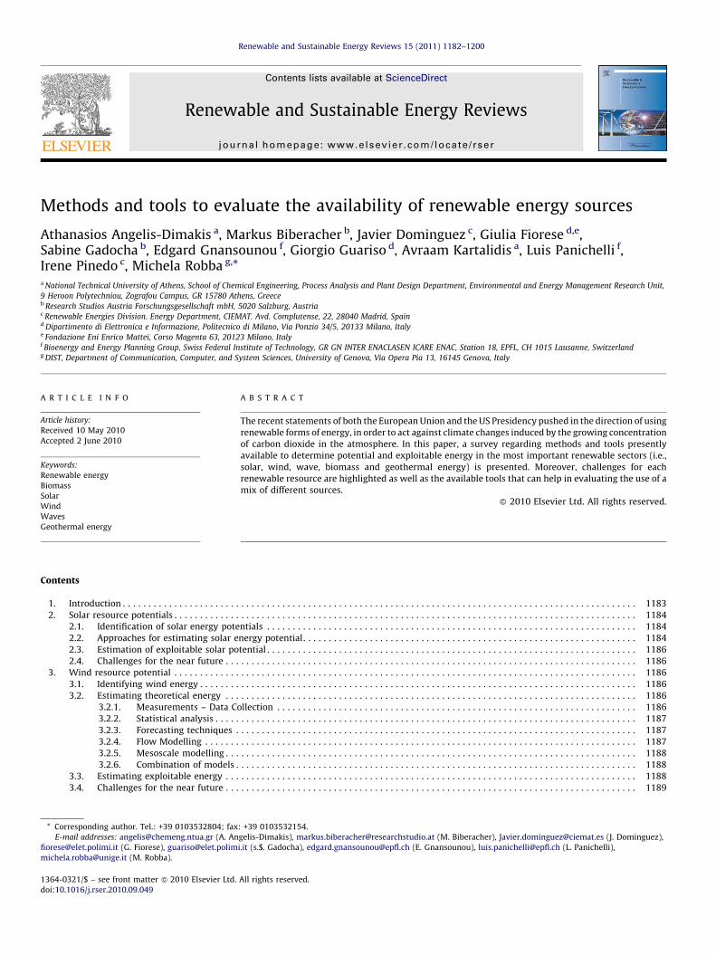
temporal resolution is 30 min, the new generation of satellites (e.g.MSG) can provide data at a temporal resolution of 15 min and aspatial resolution of 1 km [10,11]. Rigollier et al. [12], in agreementwith other authors, points out that, for satellite data with pixelsizes of 10 km, the assessment of solar irradiation provides moreprecise values compared to results of estimates by interpolation ofmeasurements from meteorological stations as soon as thedistance between the stations is greater than 34 km for hourlyirradiation values, and 50 km for daily values. A widely usedmethod within this approach is the Heliosat method, which wasoriginally implemented by Cano et al. [13] and modified by Beyeret al. [172] and Hammer [10,177]. The method has been furtherimproved by Rigollier et al. [12], implementing the Heliosat2method. The software for Heliosat2 is freely available atwww.helioclim.net. The latest evolution, Heliosat3, is presentedin Mueller et al. [178] and Betcke et al. [14].

The third and most frequently applied approach uses measure-ments from meteorological stations as well as satellite data.Satellite derived data are used for areas with an unsatisfactoryspreading of meteorological stations, as done in the Meteonormdatabase [8] or in the PVGIS (see below) approach.

There are several databases presenting solar radiation data fordifferent extents (global, continental). The list shown in Table 2.1 isnot exhaustive but shows a selection of databases for global, crosscontinental and European extents. Input is taken from Suri et al.[11], who have compared several of the existing databases on solarradiation. Beside the differences regarding the extent and thegeneral methodological approach, also the calculation of primaryand derived parameters on solar radiation as well as the temporaland spatial resolution differs between the databases. In thefollowing, three representative databases are described in moredetail.

The Meteonorm database [8] is based on a 3D inverse distanceinterpolation of measurements of solar radiation data frommeteorological stations and includes data on global solar radiationas well as the direct and diffuse fraction on a global extent. Satellitedata are used for areas with a low density of meteorologicalstations. The time resolution for interpolated measurement data isa month. Hourly and minute values can be generated from monthlyaverage values using stochastic models. Global and diffuseradiation on inclined surfaces including skyline effects can becalculated, in addition to horizontal surfaces. Influences of terrainshadowing are already included. The time period covered is 1981–2000. The database is a licensed product and is available forpurchase at www.meteonorm.com.

The PVGIS (Photovoltaic Geographic Information System) [1,15]database includes monthly averaged values of solar radiation andambient temperature for Europe. It processes climatologic datathat are available within the European Solar Radiation Atlas byusing interpolation techniques and the r.sun model. This model isimplemented in GRASS GIS, an open source environment based onC programming language. With the model, direct, diffuse andreflected fractions of solar irradiation can be calculated forhorizontal and inclined surfaces. The model also considersshadowing due to local terrain features, by integrating a digitalelevation model. The spatial resolution of the derived raster mapsis 1 km � 1 km. Further improvements for global radiationestimates of the model can be achieved by the integration of a100 m resolution digital elevation model [11,16]. Data are freelyaccessible at http://re.jrc.ec.europa.eu/pvgis/.

The HelioClim 2/3 databases contain long time series of solarradiation data for Europe and Africa. Meteosat satellite images areused to derive global irradiation maps on a horizontal surface [17].The estimations are based on the Heliosat2 method [12], whosesoftware is freely accessible at www.helioclim.net. With theHelioclim3 database, the temporal and spatial resolution could be

http://www.helioclim.net/

http://www.meteonorm.com/

http://re.jrc.ec.europa.eu/pvgis/



enhanced thanks to the new Meteosat Second Generation satellites[10]. The Helioclim3 database has a temporal resolution of 15 minand a spatial resolution of approximately 5 km. Data are availablefrom 2004 to 2007 [18].

2.3. Estimation of exploitable solar potential

Following the described top down approach, the available solarpotential is further reduced to what is economically exploitable, bythe integration of restricting factors regarding suitable areas,technical and economical factors ([5,6,19]). Geographical restric-tions for the installation of solar energy systems are included toderive only suitable areas, by using land cover maps. Thisevaluation also depends on the type of solar installations.Hoogwijk [5] shows how to identify suitable areas for centralisedand decentralised PV systems. While centralised installations withgrid connection are assumed to be installed on land surface,decentralised applications are assigned to roofs or facades.Concentrating Solar Power (CSP) for instance is most suitable inbare areas with a high share of direct irradiation. On a global orregional scale, current land cover datasets are satisfactory for theestimation of suitable areas, on a local scale, analyses may requireto go down to the single roof top. One approach for the estimationat such a detailed level is the use of Laserscan data [20,21].

Other local factors may play a role in the detailed estimation ofthe performance of solar energy systems. Huld et al. [15], forinstance, presented a method taking into account the influence oftemperature. More frequently, however, typical efficiencies for thedifferent solar system types are applied, following the state of the art[5,6], and determine whether the spatial constraints can be satisfied.Finally, economic factors can also be essential to determine thefeasibility of a project, as shown again by Hoogwijk [5].

All in all, available databases and relevant restriction factors canbe identified within a 2 dimensional matrix representing the globalto the local scale as well as the theoretical to the economicallyfeasible potential scale. All methods and data sources can belocated somewhere in between (Fig. 2.2).

2.4. Challenges for the near future

A cross comparison of six databases for solar radiationestimates carried out by Suri et al. [11] showed that, in the caseof yearly sum of global irradiation, the uncertainty, expressed bystandard deviation, does not exceed 7% within 90% of the studyregions for horizontal surfaces. Especially for mountain areas with

[()TD$FIG]

Fig. 2.2. Matrix of available databases and restricting factors covering the spatial

dimension as well as the dimension of the top-down levels.

their complex climate conditions, higher differences between thedatabases are expected. Therefore further improvements forcomplex terrains should be done.

Compared with other renewable energy carriers like wind andbiomass, solar energy can be also harvested in densely populatedareas. Approaches and methods to derive an effectively exploitablepotential are still in a process of evolution (e.g. laserscan data likeLIDAR), but the opinions on what potential is really harvestableunder sustainable conditions are quite diverse. Further improve-ments can be expected mainly in the explicit mapping of suitablerooftops regarding orientation and inclination, including alsoshadowing of neighbouring parts of buildings or trees. Especiallythe competition for installation areas between different solar systemtypes (PV, solar heating) in case of decentralised usage have to beincluded in potential estimations, as the efficiencies of these systemsdiffer substantially as well as the final energy use: electric energy canbe returned to the grid, when not used; while thermal energy can beexploited only locally and with a limited storage capacity.

3. Wind resource potential

Wind was one of the first energy sources to be harnessed byearly civilizations. Wind power has been used to propel sailboatsand sail ships, to provide mechanical power for grinding grain inwindmills and for pumping water. The world’s first automaticallyoperated wind turbine, which was built in Cleveland in 1888 by C.F.Brush, was 18 m tall and had a 12 kW turbine [22]. Nowadays theuse of wind energy in electricity generation is widely spread andnew units with nominal capacity of thousands of megawatts arebeing installed each year. The total wind power capacity installedworldwide has exceeded 120 GW in 2008 [23]. The ever increasinginterest for wind energy, coupled with its uncertain nature, makesthe estimation of wind energy perhaps the most difficult andcrucial part of a project.

3.1. Identifying wind energy

As for solar power, the evaluation of the available wind energyfollows a widely used top down approach. At the first level, thepotential energy limited by all the physical geographical (highaltitude areas, high slope areas), socio geographical (areas neartowns, airports or archaeological sites, protected areas) and landuse (areas used for agriculture, etc) constraints leads to theestimation of the theoretical energy.

This can be assessed at a scale of the order of few kilometers,simply by processing the available anemological data (long orshort term), with either statistical models or interpolatingtechniques. The latter are used mainly when sufficient data arenot available for the site of interest, but only for nearby ones. Whenthe estimation scale needs to be much smaller, of the order of a fewmeters, the methods used must be more accurate (e.g. wind flowmodelling techniques).

The theoretical energy can be further limited by the character-istics of the commercially available wind turbines (size, overallefficiency, full load hours) and the constraints of a wind farm.

Finally, the exploitable energy can be defined as the part of thetheoretical energy that can be harvested using an economicallyfeasible installation, given also the cost of alternative energysources. The basic methods used to estimate the differentcategories of wind energy are presented in the next sections.

3.2. Estimating theoretical energy

3.2.1. Measurements – Data Collection

Every effort to estimate the theoretical energy of a regionrequires the availability of certain measurements, year-long or not,


referring to either the target site or another site nearby (referencesite). According to Lalas [24], the available anemological datashould include: (i) mean wind speed, on a monthly or seasonalbasis, (ii) duration curves, (iii) persistence, i.e. continuousoccurrence of wind speeds above a given speed, (iv) wind rose,i.e. joint frequency of occurrence of specific wind speed anddirection, (v) power spectra of wind speed, and (vi) variation withheight of most of the above. Ideally, in order to obtain an accurateassessment of the wind regime of an area, wind data measure-ments over a 10 year period are required [25]. However, Frandsenand Christensen [26] claim that a 1 year period of windmeasurements may provide a reasonable indication of thepotential for wind energy development, including a percentageof uncertainty from 5% to 15%, depending on the variability of thelong term mean wind speed.

Using accurate inputs is crucial in wind resource assessment, sospecial emphasis should be given on the quality of anemologicaldata. A detailed description of the various types of equipments,instruments, site specifications and other technical needs for windenergy assessment has been presented by Alawaji [27]. Meteoro-logical towers are the most common means of assessing the windresource at a location, typically between 40 and 60 m high, withcup anemometers and wind vanes positioned at multiple heightson the tower.

Nowadays, wind maps and global databases have beendeveloped for many regions around the world, such as NCEP/NCAR and ECMWF databases, containing wind speed, temperatureand pressure at several heights around the world [28]. However,low resolution of some existing data (i.e. hundreds of km) and lackof data for certain regions (i.e. offshore) have led to thedevelopment of new techniques. Ground based remote sensinginstruments, such as SODAR, LIDAR or satellite, have started beingused as alternatives to meteorological towers for wind resourceassessment with high resolution. However, their effectiveness andefficiency will have to be proved since their possible limitations arestill under examination.

Choisnard et al. [29] and Bruun Christiansen et al. [30] present amethodology for wind resource assessment using a series ofsatellite synthetic aperture radar (SAR) images, a techniqueparticularly useful for regions where year-long time series aregenerally unavailable, such as offshore regions. Lackner et al. [31]investigate the use of an alternative monitoring strategy for windresource assessment, the ‘‘round robin site assessment’’ method.Wind resource is measured at multiple sites within a year, using asingle portable device and measurement time is distributed at eachsite over the whole year.

Data collected in any of the ways described above can then beprocessed in order to provide useful information about the windenergy. The following sections present the basic processingmethods.

3.2.2. Statistical analysis

When year-long measurements for the target site are available,they usually constitute an enormous volume of data, difficult toanalyse in its raw state. A simple solution would be to apply theproper statistical treatment in order to determine the probabilitydensity function (PDF) of the wind. The use of this frequencydistribution approach can provide a simple method to evaluate thetheoretical wind energy, because it provides useful informationabout wind speed.

Carta et al. [32] review and compare the most widely used andaccepted distributions in the specialized literature on wind energyand the methods utilized to estimate their parameters. Theyconclude that the Weibull distribution has a number of advantageswith respect to the other PDFs analysed. However, Weibull cannotdescribe all the wind regimes encountered in nature such as, for

example, those with high percentages of null wind speeds, bimodaldistributions, etc. Therefore, despite there are numerous examplesin the literature of using the Weibull distribution for regional windenergy estimation, how to select the appropriate PDF for each windregime in order to minimise estimation errors is still an openproblem.

Stevens and Smulders [33] obtained the values of the Weibulldistribution parameters using five different methods: moments,energy pattern factor, maximum likelihood, Weibull probabilityand the use of percentile estimators. The comparison of theseanalytical findings indicated that no significant discrepanciesbetween the results from the different methods could be observed.

A Cumulative Semi Varigram (CSV) model has been derived bySen and Sahin [34] to assess the regional patterns of wind energyalong the western Aegean Sea coastal part of Turkey. Thisinteresting technique provides clues about regional variationsalong any direction and yields the radius of influence for windvelocity and Weibull distribution parameters.

3.2.3. Forecasting techniques

When the available anemological data for the target site areinsufficient, the measure–correlate–predict (MCP) methods can beused to estimate the theoretical wind energy. These algorithms canreconstruct the wind resource at target sites by using data from anearby reference site. The idea is to correlate short termmeasurements at the target site with an overlapping long timeseries of the reference site using simple statistical models.According to Landberg et al. [28] climatological representativenessis obtained by having measurements for at least 5 but preferably 10years.

The way the correlation is established between the wind speedat the two sites varies from method to method. A linear regressionmodel is used in many cases, but other models are used as well.Rogers and Rogers [35] describe some of the MCP approaches in theliterature and then compare the performance of four of these, usinga common set of data from a variety of sites (complex terrain,coastal, offshore).

Addison et al. [36] state that conventional MCP techniquesassume that the wind direction distribution at the target site is thesame as that of the reference site, which may lead to a significanterror and propose a correlation technique based on artificial neuralnetworks (ANN). Bechrakis et al. [37] present a two site windcorrelation model, also based on an ANN, in which concurrentmeasurements of a short time period for both sites are beingprocessed.

3.2.4. Flow Modelling

The techniques described in the previous sections estimate thetheoretical wind energy at a resolution of the order of fewkilometers, in the best of cases, suitable for a raw evaluation of thewind potential of a region. However, when wind turbineinstallation is designed, the resolution should be of the order offew meters and hence wind flow models are employed.

Based on the theory of flow over small hills, some linearizedflow models were the first to be developed for commercial use. Inthese models, the equations of motion were simplified bylinearizing the advection terms and the other weaker nonlinea-rities in the turbulence closure equations [38]. Indicative examplesof such models are the WAsP model [39], based on some linearizedforms of the fluid flow equations, and the MS Micro model [40].

A significant application is Wind Atlas methodology [39], amethod of vertical and horizontal extrapolation away frommeasurements taken somewhere within or near a target site,using steady state flow solutions (Fig. 3.1). The method directlycorrects existing long term measurements and estimates thegeneralized wind climate, the hypothetical wind climate for an

[()TD$FIG]

Fig. 3.2. Downscaling using mesoscale and microscale modelling. Adapted from

[169]

[()TD$FIG]

Fig. 3.1. Wind atlas methodology. Adapted from [39]


ideal, featureless and completely flat terrain with a uniform surfaceroughness, assuming the same overall atmospheric conditions asthose of the measuring position. This method can also be used inreverse, in order to determine to a high accuracy the specific windsat a site. This methodology, combined with WAsP, has been appliedin a large number of countries (all of EU countries, Russia, NorthernAfrica), because of the modest computer resources requirementshas become a de facto standard for the wind industry [41].

The main disadvantage of linear models is the low accuracy inthe calculations of wind conditions in steep/complex terrain withknown overestimates of the hill top acceleration and under-estimates of the lee side decelerations [38]. Another problem isthat thermally driven winds are not modelled in a satisfactory way,especially with the Wind Atlas Methodology [28].

These limitations are becoming significant, since the pressurefor increased wind capacity is leading to the installation of windfarms even in areas of increased terrain complexity. In such cases,more complex nonlinear models permit overcoming many of theshortcomings mentioned above, and also provide a more accuraterepresentation of the case under consideration. The most popularnonlinear model is RaptorNL, a computational flow model thatsimulates turbulent flow over topography.

Palma et al. [42] evaluate the theoretical wind energy of acoastal region using a wide variety of techniques, including fieldmeasurements and computer simulations using linear andnonlinear mathematical models and compare the results.

3.2.5. Mesoscale modelling

A different type of models, which began to emerge as a majorfocus of research during the late 1990s, are atmospheric mesoscale

models. They were developed for general weather prediction atfine resolution (1–10 km) and in particular for air pollution studies,and aviation purposes. They can be applied to estimate the windresource of a region, by solving numerical equations for theconservation of momentum, heat and moisture, together with acontinuity equation.

Lyons and Bell [43] used a numerical mesoscale model todescribe the variation of wind energy across a coastal plain ofWestern Australia and to compare the results with those of asimpler linear flow model. Katsoulis and Metaxas [44] use a massconsistent numerical mesoscale model to estimate the theoreticalwind energy in Corfu, Greece, comparing the results with thestatistical analysis of wind data from local meteorological stations.The major problem of mesoscale modelling is that resolutions of1 km or less require a very high computational effort.

3.2.6. Combination of models

A way to overcome this problem is the use of mesoscale modelsin combination with a wind flow model (microscale model).Instead of trying to resolve all small scale terrain features, themesoscale modelling stops at a resolution of approximately 5 kmand local predictions are made with a wind flow model (Fig. 3.2).

Frank and Landberg [45] use the Karlsruhe AtmosphericMesoscale Model, combined with the linear wind flow modelWAsP, to estimate the theoretical wind energy of Ireland. Broweret al. [46] develop MesoMap, a combination of MASS mesoscaleatmospheric model and microscale model WindMap, and apply itfor the estimation of theoretical energy in several areas in USA.Pepper and Wang [47] use the PSU/NCAR fifth generationMesoscale Model (MM5) in conjunction with an h-adaptive finiteelement model in order to conduct wind energy assessment incentral Nevada. Kondo et al. [48] use a mesoscale model (AIST-MM) combined with a multi layer canopy model to estimate windenergy in an urban area.

3.3. Estimating exploitable energy

There is no definite methodology referring to the estimation ofexploitable energy. Hence, certain indicative examples of itsestimation will be mentioned, at various scales, regional, nationalor even global. Voivontas et al. [49] attempt to estimate thetheoretical and exploitable wind energy in a Greek island, using aGIS Decision Support System (DSS). Acker et al. [50] use GIS andwind maps, created by a mesoscale wind energy model, to producea wind resource inventory in the state of Arizona, to evaluate themost promising sites for wind development and to present the costof energy by using the NREL wind energy finance calculator.Hoogwijk et al. [51] present the assessment of the globaltheoretical and exploitable wind energy, performing a sensitivityanalysis for uncertain assumptions. de Vries et al. [52] investigatethe potential of wind, solar and biomass, focusing on uncertaintiesin land use cover, by building four different scenarios. Biberacher


et al. [3] developed a global GEOdatabase, including all renewableenergy resources, at high resolution taking into account competi-tive land uses.


According to Petersen [53], a point has been reached where bygiving the coordinates at any spot on Earth, the local wind energycan be estimated with a reasonably well known uncertainty. Thishas been made possible due to model development, where linearwind flow models are combined with adapted nonlinear modelsand mesoscale meteorological models, to fully exploit thecapabilities of each method.

The greatest challenge for wind resource estimation is to findflow models and numerical schemes which can pick up the mainfeatures of the wind flow in complex terrain and/or very complexclimatology while keeping the calculation effort at an acceptablelevel. Other challenges are related to the prediction of theturbulence conditions and extreme winds at specific sites andthe reduction of the uncertainties in the estimates. Ayotte [38]presents the most recent developments and the challenges whichstill exist in flow modelling for wind resource assessment.

With respect to the huge potential of planned offshore farms,research attention has shifted to the estimation of the offshorewind potential. Many papers have been written on this subject inthe last years [54–56]. The question that needs to be answered iswhether the methodologies mentioned above can still besatisfactorily used for this purpose, given the unique features ofthese cases (strong thermally driven wind flow, sea surfaceroughness, bathymetry). Finally, recent studies have been initiatedto consider the effect of climate change on the wind potentialenergy [53].

4. Wave energy potential

The worldwide wave energy potential is estimated of the sameorder of magnitude as the world electrical energy consumption,however power generation is not currently a widely employedcommercial technology. Some of the earliest recorded attempts toconvert wave energy into more usable forms date back to severalcenturies, and today, thanks to the offshore oil industry andoffshore wind energy development, much of the infrastructure andknowledge necessary to efficiently generate energy from the oceanalready exists. Several wave energy conversion devices havealready demonstrated the potential for commercially viableelectricity generation and are expecting pre-commercial deploy-ment in Europe. However, in order to achieve competitiveness, agood understanding of wave climate at the installation site andweather forecasting techniques are necessary.

4.1. Identifying wave energy potential

As already pointed out, wave energy can be considered as aconcentrated form of solar energy. The differential heating of theearth generates winds which transfer some of their energy to formwaves as they pass over open bodies of water. Waves travel greatdistances without significant losses and so act as an efficientenergy transport mechanism across thousands of kilometers.

Whatever the means used to record or predict a wave climate,the sea state is usually described by using a simplifying set ofstatistical parameters. A sea state can then be represented as aspectrum of regular waves and often summarized in terms of waveheight spectral peak, dominant wave period and mean wavedirection. These wave spectral parameters are then used toquantify the wave energy resource and to estimate the flux ofenergy per unit of wave crest. The variation in sea states over a

period of time can be represented by a wave scatter diagram,which indicates how often a sea state with a particularcombination of wave height and period occurs. The angulardistribution of wave power is usually represented in a ‘‘wave rose’’.Synthesizing, the statistical parameters used are very similar tothose adopted for wind energy.

Wave energy is a renewable resource and therefore it isvirtually inexhaustible in duration but limited, and also highlyvariable, in the amount that is available per unit of time. Thetheoretical potential identifies the physical upper limit of waveenergy available at a certain site. The technical potential takes intoaccount restrictions regarding the state of the art of the technology,limiting the theoretical potential and reducing the area that isrealistically available for energy generation. The potential isfurther reduced when additional but compulsory restrictions aretaken into account such as the proportion that can be utilisedrespecting ecological and socioeconomic factors. The methodsused to estimate these potentials, along with several examplesfound in the bibliography, are described in the following sections.

The World Energy Council has estimated the worldwide wavepower resource in deep water between 1 and 10 TW [57]. As mostforms of renewables, wave energy is unevenly distributed over theglobe, varying by location and time. The best wave climates interms of increased wave activity, with annual average power levelsbetween 20 and 70 kW/m of wave front, are found in the temperatezones (30–608 latitude). However, attractive wave climates arealso found within equatorial zones (0–308 latitude) where regulartrade winds blow and the lower power levels are compensated bythe smaller wave power variability.

Although the scale and character of the wave energy resource inmany regions around the world remain poorly understood and illdefined, especially in nearshore areas, several efforts have beenmade to estimate the wave energy potential at regional, nationaland global scale. Some of them are described next, groupedaccording to the methods used and to the sources of data.

4.1.1. Direct and remote measurements

The most realistic wave data is collected in situ using mooredbuoys, fixed structures (laser and acoustic sensors) and bottommounted pressure and acoustic sensors. The most common systemis buoys. In the past, they could only measure wave energy but inthe last years buoys equipped to measure horizontal surge andsway motions are used, allowing the calculation of wavedirectionality. Some wave recording buoys have been collectingdata for years, gathering useful long term series.

However, these types of measuring systems are not widelyavailable and do not have a worldwide evenly distributed cover,mainly due to high costs and difficulty related to harsh environment.

Satellite technology has started being used for accuraterecording of wave height, velocity and direction, including bothlocal and localised effects. It is not sensitive to bad weatherconditions, but has low frequency of measurements and relativelyhigh distance between tracks as drawbacks. Krogstad and Barstow[58] describe the methodology used to calculate wave height, windspeed and wave period over 15 years based on satellite data. Theypresent several case studies and also provide a few Internet siteswhere satellite wave data can be found. Barstow et al. [59] usedtwo years of altimeter data to construct a global map of theavailable wave energy resources in deep water. Despite therelatively short record length, the analysis succeeded in generatingreasonable estimates of the spatial variation of mean wave energy.

Satellite observations are able to provide reliable global longterm wave statistics, also contributing to improve short term wavepredictions. Combined with short term forecasting techniques,these data could be used to modify controlled response for safety inapproaching storms and to call for dispatch balancing plant in the


electricity network to accommodate reductions in wave energyproduction.

4.2. Statistical analysis and numerical models

Measuring systems produce a huge quantity of data that couldbe difficult to evaluate in its raw state. In order to help in thehindcasting and forecasting of wave climate, a more or lesscomplicated statistical analysis is generally applied. Regarding thehindcasting of wave climate from meteorological data, Smith et al.[60] proposes a new statistic that measures the rate of change inthe wave period from one wave to the next, which would berelevant to wave energy devices. Statistical analysis could also helpto determine the long term resource potential for a given site. Thiscan be used to evaluate a site for development viability, but will notwork for predicting the energy produced.

According to Rusu and Guedes Soares [61], wave energy can beaccurately predicted within a window of a few days not by statisticalanalysis, but by using numerical models, the most widely used ofwhich are WAM (Wave Analysis Model), WAVEWATCH III,FUNWAVE and SWAM (Simulating Waves Nearshore Model). Theymodel wave generation based on wind-wave models, wavepropagation and transformation, from open ocean to within portsand harbors. While WAN, WWIII and FUNWAVE are used at globalscale for offshore locations, linking meteorological parameters toproduction of ocean wave regimes, SWAN is used to introduce thewave transformations that occur near the coast (whitecapping,bottom friction and depth induced wave breaking) [62].

Several authors have reported detailed energy resourceassessments for particular regions or countries: Ireland [63],United Kingdom [64], Portugal [65], California [66], Canada [67],the Baltic Sea [68]. These types of studies involve analysis of wavedata from buoys, satellites, numerical wave hindcasts or acombination of these sources.

4.3. Estimating technical potential

Wave power estimates usually describe the energy flux due towave propagation but only a fraction of the energy flux available atany site can be captured and converted into more useful forms ofenergy. This fraction is imposed by the wave energy converter(WEC) inherent power limitation. How to calculate the fraction of‘‘extractable’’ resource is not yet well established since there is notan agreement on the optimum wave energy conversion mecha-nism.

It is also necessary to consider the effect of the resourcevariability on device performance since the excess wave power insea states larger than a threshold power level is unexploitable. Thisthreshold will depend on device/wave farm hydrodynamics, but inthe case study presented by Folley and Whittaker [62] four timesthe average incident wave power has been used. They present amethod to estimate the wave energy resource in nearshore areas,proposing a measure of the resource that represents moreaccurately the potential for exploitation, avoiding omnidirectionalwave energy and discounting high energy sea states.

Boehme et al. [69] suggest some figures of the loss in electricityproduction (and therefore, the reduction of theoretical resource tothe extractable potential) generated with a Pelamis type device inScotland.

4.4. Estimating economic and sustainable potential

Most of the examples found in the literature agree on therestrictions that must be considered in order to estimate therealisable wave energy potential and how to rank feasible locationsfor wave energy deployment. Some suggest how the costs could be

reduced, and several defend GIS as an appropriate tool to jointlyevaluate the social, economic and environmental constrains. Forinstance, Henfridsson et al. [68] examines possible examples ofpower installations in the Baltic Sea. Activities such as commercialfishing, shipping channels, areas of military interest, sites ofmarine archaeological importance and valuable biological reserveswere taken into account in the definition of the feasible areas. Alsogeographical conditions were considered, such as distances fromland and grid, the depths and substrate of the seabed, which can setboundaries to what is economically feasible.

In the case of Boehme et al. [69], GIS technology was used as thecomputer environment within which renewable resources, alongwith most of the physical constraints on their development, weremapped. The GIS program was also used to model renewableelectricity generation, establishing the spatial relationshipsbetween resource, generation and electrical load datasets.

The method presented in Nobre et al. [70] constitutes areference example in performing geo-spatial analysis aiming toidentify the best location to implement a wave energy farm offPortugal coast. Several factors, such as technological limitations,environmental conditions, administrative and logistic conditions,are taken into account. Some restrictions are imposed in theanalysis (exclusion zones) while other areas have their suitabilityranked with weighting factors. The result is a spatial suitabilityindex for farm deployment.

The cost involved in transmitting power to the electricitynetwork from an offshore location is clearly more expensive thanfrom an onshore location, due to the underwater cable infrastruc-ture. Prest et al. [71] describe a method, based on GIS, whichoptimises the cable route between a wave farm and the electricitynetwork, while taking a range of exclusion zones. Graham et al.[72] also use techniques available through GIS to optimise theintegration of marine energy into the electricity network.


For most wave energy conversion mechanisms, it is necessaryto tune the oscillating bodies to some period of the waves. Hence, agood understanding of the wave climate at the site is required. Abetter resource analysis and weather forecasting is one of the mostimportant challenges faced by marine renewable resources [73] inorder to achieve competitiveness. It is also important to producegood and reliable information on the steadiness of the wave energyresource throughout the year and on the severity of the waveclimate extremes when conducting resource assessments for waveenergy projects, since production and survival of converters willrely on them.

It will be critically important to ensure that the development ofnew ocean energy technologies do not harm the marine environ-ment, taking into account all the environmental restrictions thatwould assure the sustainability of its exploitation, while theresource assessment is performed. Recent studies have alsosuggested the necessity of considering, in long term planning, theimpact that climate change could have on the marine resources [74].

5. Dry biomass and energy crops potential

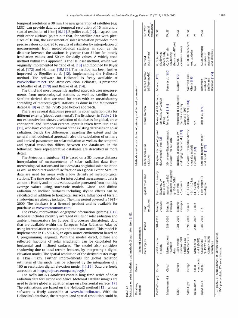
Biomass resources have been largely used as traditional fuelsand are now being promoted as a strategy to achieve sustainabledevelopment. Biomass is mainly available locally, allows thewidespread production of energy at reasonable costs and can helpto mitigate climate change, develop rural economies and increaseenergy security. Consequently, several methods and tools havebeen developed to assess the availability of biomass resources. Wefocus in this section on methods and tools for biomass estimationat the regional level subdivided by biomass type.


Biomass is defined as the biodegradable fraction of products,wastes and residues from agriculture, forestry and relatedindustries, as well as the biodegradable fraction of industrialand municipal wastes. Moreover biomass can be grown on purposein dedicated energy crops. Residual biomasses derive from:

� the agricultural sector, both in the form of crop residues and ofanimal waste;� the forestry sector, from forests’ thinning and maintenance;� the industrial sector of wood manufacture and food industries;� the waste sector, in the form of residues of parks maintenance

and of municipal biodegradable wastes.

Biomass potentials are classified depending on their theoretical,techno-economical and sustainable availability. The theoreticallybiomass potential can be estimated on the basis of biophysical andagro-ecological factors that determined the biomass growth andextension and the residues production ratios. The techno-economical potential is then estimated taking into accountaccessibility, resources competition, biomass logistics, productioncosts and all other factors that constraint the theoretical potential.Sustainable potential is a further assessment that aims atevaluating the amount of biomass that can be obtained consideringsocio-economical and ecological impacts of this type of energyprojects. Constraints may vary according to regional specificitiessuch as forestry, agricultural and industry practices, to socio-economic conditions and to the natural environment.

We will first consider dry biomass, namely that with a humiditycontent below 30%, and analyse specific methods to estimate thepotential of different sources, namely, woody biomass, agriculturalbiomass, energy crops and industrial residues.

5.1. Estimation of biomass potential

5.1.1. Woody biomass

Woody biomass estimation methods are usually based on forestinventories and agricultural censuses. The theoretical potential ofbiomass in forests is typically estimated through biomassallometric regression equations (BARE) and biomass expansionfactors (BEF) [75]. Allometric equations are regressions that relatediameter and height of a tree to stand volume and total biomassvolume [76]. A vast bibliography is available presenting allometricequations (e.g. [77,78]). Local and regional characteristics such asclimatic variables and topography have a strong influence in forestgrowth and so in the aboveground biomass volume. Specificallometric equations should be developed for each tree species, foreach forest development stage and for each region. As these valueshave not been computed for all interesting species and locations,many authors adjust equations available in literature.

BEFs are used for total aboveground biomass estimations andtheir components as an intermediate step for carbon stock andchange calculation in forests. BEFs convert timber volumes towhole tree biomass and are calculated as the ratio betweenaboveground biomass and stem volume [79]. Some controversieshave arisen regarding BEFs use for biomass estimations such as itsinapplicability to trees below merchantable wood [80], and BEFstatistical error is often unknown leading to biased estimates.Efforts are being done to obtain more accurate BEF [81] includingthe differentiation by age and the estimation of error, but theycannot be applied when stand development conditions deviatefrom those under which the BEFs were computed [82].

Forest treatments, mainly pruning, thinning, and final fellingare a key element as annual forestry residues production dependson these factors. Esteban Pascual [83], Panichelli and Gnansounou[84], Panichelli and Gnansounou [85] give examples of biomassestimations based on forest management practices.

The main uncertainty in estimating woody biomass potential isthe difficulty to account for forest dynamics. The last century hasseen the development of various models for this purpose. Suchmodels have been developed following different approaches andvary from complex eco-physiological models, suitable for the studyof the impact of forest on climate change, to empirical models.Forest growth models generally can be classified within thefollowing categories [86,87]: (a) highly aggregate volume over agemodels, used for regional yield forecasting; (b) stand models, usedto predict the growth as a function of age; (c) size class models,used to predict the plants growth in terms of variations of thediameter distribution; (d) individual tree models that provideinformation about the plant growth, on the basis of spatialrelations. Some models of forest growth [88] dynamics have beendeveloped but not fully integrated in biomass potential estima-tions. One of these is CO2FIX [89,90] that has been designed toestimate all carbon flows from the atmosphere to the standingbiomass, from biomass to decay in the soil, from the soil back to theatmosphere. These flows describe, through many parameters, thenatural dynamic of a forest. Moreover, flows can be added toaccount for forest management (cuttings and crop rotations) andfor the use of the woody products.

5.1.2. Agricultural biomass

The theoretical potential of crop residues can be estimated onthe basis of the cultivated area or the agricultural production foreach crop (usually available from regional or national statisticaloffices) and average product to residue ratios or residue yieldsderived from literature or from referenced local trials. Differentauthors have proposed product to residue ratios [91]. This methodhas been widely applied to estimate agricultural residuesavailability for energy purposes [92,93]. The residue availabilitymay significantly vary with local agricultural practices andclimatic conditions. Product to residue ratios should thus beestimated at regional level on the basis of field trials [94].

The theoretical potential of agricultural residues for energypurposes is restricted by competition and logistics constraints.Almost half of the total agricultural residues are exploited in non-energy applications [95]. Moreover, agricultural machineries arenot able to collect all the residues from the soil and typically leave40–50% of it on the field [96].

Moreover, crop residues play an important role both protectingsoil from erosion and returning nutrients to the soil. Residuesremoval should be evaluated in each specific case, according tolocal soil and climatic characteristics and to agricultural practices.In the USA this a very important issue given the high soil erosionrates experienced in the central plains, where wind, wateravailability and soil conditions strongly affect the amount ofresidue removal, as modelled by Graham et al. [97]. Agriculturalresidues have to be collected and transported to the conversionplant. Since the bulk density of agricultural residues is generallylow, transport costs can be significant and need to be carefullyassessed. One way to contain transportation costs is to processresidues and densify them, for instance by baling.

5.1.3. Energy crops

Biomass can be supplied by dedicated agricultural crops ofarboreous and herbaceous species: short rotation forestry (SRF, e.g.poplars, willows, eucalyptus), annual crops (e.g. corn, soy, sugarcane, sorghum) and perennial grasses (e.g. switchgrass, mis-canthus). Several models have been developed to support thedecision over which species to grow. Local climate, morphology,soil characteristics, water and nutrients needs are commonly usedto identify the set of species suitable for a specific area [98]. Forexample, potential biomass productivity of tree species can beassessed on the basis of the FAO/IIASA Agro Ecological Zones

[()TD$FIG]

Fig. 5.1. Classification of biomass potentials.


approach [99], while some information for herbaceous species canbe found in the ECOCROP database (ecocrop.fao.org/).

Eventually, the most important issue regarding energy crops isthe assessment of available land. Some models have presentedassessments of land availability at global level [100]. However,once at regional scale different methods are needed in order toaccount for local socio-economic and environmental conditions.Land available for energy crops can be identified with the help ofcurrent land use data and statistical databases. However, landconversion costs, social concerns and environmental constraintsmay limit the amount of available land for energy crops. Given a setof species suitable for a given area, an optimization problem of theentire energy chain (including cultivation and transport) must besolved in order to determine the amount of land to be dedicated toeach specific crop [101].

A different approach for estimating energy crops potential is theeconomic modelling of the entire agricultural sector. Economicmodels account for biomass production for the internal market,exports and imports, and detailed costs and benefits of the majorfarming goods. The Polysis model [102], developed for the USAestimates biomass production on the basis of the net profitscompared with those derived from conventional crops. This modelrelies on many assumptions that range from farming practices tomacro-economic variables of the agricultural sector.

GIS based applications allows considering spatial patterns ofbiomass distribution. Graham et al. [103], Graham et al. [104]developed a regional scale GIS based modelling system forevaluating potential biomass production and costs from energycrops.

5.1.4. Industrial residues

Biomass from industrial residues includes wood from sawmillsand timber mills and by products of the food industry. Theprinciple of waste reduction, re use, recycle and recover should beconsidered also when proposing waste to energy projects.

Municipal solid waste, liquid by-products from the pulp andpaper production industry; food processing wastes can all be usedfor energy conversion, in some cases together with the wetbiomass, as discussed in the next chapter.

The availability of information on quantities of currentbiowaste production may significantly differ across the wastestreams. Municipal solid wastes are monitored by government, sothat statistics about their availability and the type of waste shouldbe easily recovered from the national statistical offices. Similarly,the industry and service sectors are normally required to notify thetype and the amount of waste produced, according to thecategories of waste.

Solid industrial residues consist mainly of clean wood fractionsfrom the secondary wood processing industry. These residues arealready concentrated at a processing industry and are often alreadydried, which reduces logistic and pre-treatment costs. However,wood industries already use part of these residues for heatingpurposes, so that the final amount of wood residues available forother energy conversions is reduced. Wood industrial wastes canbe estimated from the quantity and quality of wood processed andfrom the type of process that the wood undergoes. The actualquantity of residues depends on several factors, such as woodproperties, type of operation and maintenance of the plant. Again,alternative uses of wood residues, such as chips for pulpproduction, raw materials for particleboard and fibreboardproduction, must also be considered (Fig 5.1).

5.2. Spatial patterns and optimization

State of the art in biomass to energy planning is focused on GISbased approaches where biomass potential is estimated from geo-

references inventory data. Once that the available potential ofbiomass is assessed, the system is optimized based on costminimization of biomass production and utilization in energyconversion facilities.

Satellite images have been widely used to assess spatialpatterns of biomass production. Methods account for the integra-tion of forest inventories with satellite imagery [105,106], the useof LIDAR remote sensing data [107], teledetection applications[108] and normalized difference vegetation index (NDVI) dataprocessing [109].

One of the main issues is the distance of the conversion plantfrom the needed feedstock and the capacity of the plant itself.Given a certain biomass availability and regional distribution, atthe increase of size, in fact, collecting distances increases and thusalso the biomass supply costs [110–112]. Many models haveevaluated these issues, among them the Biomass ResourcesAssessment Version One (BRAVO) system in a computer basedDSS to assist the Tennessee Valley Authority in estimating thesupply cost for wood fuel as a function of the hauling distances[113]. In this type of analysis, spatial information is needed in orderto know where to collect the biomass from and where to deliver it.

Interactions of biomass supply and demand have also been amajor subject of research. Masera et al. [114] have assessed thewood fuels resources in Mexico, Slovenia and Senegal using theWoodfuel Integrated Supply/Demand Overview Mapping model(WISDOM). The model is a GIS based tool aiming to analysefirewood demand and supply spatial patterns highlighting areas inwhich several criteria of interest coincide.

Much of the present work is directed toward the developmentof GIS based decision support tools of the complete biomass-to-energy chain, such as that developed by Frombo et al. [115],Frombo et al. [116]. Another GIS based model for public forests,based on inventory data, was developed and tested in the NorthernBlack Forest region, Germany [117]. The feasibility of the biomassto energy chain was assessed in the Tuscany region [118].Tatsiopoulos and Tolis [119] have evaluated the economic aspectsof the cotton stalk biomass logistics in a mathematical formulationfor Thessally, Greece. Centralized and decentralized approacheswere considered and the entire model was driven by a GIS interfacethat permitted to define the suitable location for siting powerunits. These tools are useful to identify the main parameters that

http://ecocrop.fao.org/


affect location and number of bioenergy conversion facilities basedon plant capacity and spatial distribution of the available biomassresources.

DSSs may also allow policy makers to assess the impact ofbioenergy policies: Chalmers et al. [120], for instance, have createda GIS based tool that estimates the effect of policy constraints inthinning.

Finally, they may explicitly include economic considerations.Kinoshita et al. [121] have focused on the spatial modelling offorest biomass as a function of production costs for differentmachinery and forest treatment. An integrated GIS based approachincluding techno-economical, socio-political and environmentalconstraints to biomass production and utilization was developedby Perpina et al. [122] to evaluate biomass to energy potential inthe Valencia Community, Spain. Panichelli and Gnansounou [84],Panichelli and Gnansounou [85] have tackled the problem ofresources competition between energy facilities and farm gateprice variability in function of biophysical and location constraints.The DSS model was applied in Northern Spain to determineoptimal locations for bioenergy facilities.


The main challenges in biomass to energy planning deal withthe improvement of models to account for forest and agriculturaldynamics and their integration into GIS environments, thedevelopment of specific biomass estimation factors and equations,the assessment of biomass competition between energy conver-sion and other uses, and the development of multicriteriaoptimization models. Moreover, social and environmental consid-erations [123] need to be taken into account in order to face issuessuch as biodiversity loss.

6. Wet biomasses and biogas potential

In this section of the paper, we will analyse biogas productionvia anaerobic digestion (AD). Biogas produced via AD is a mixture ofmethane (CH4) and carbon dioxide (CO2), in a ratio of about 60/40to 70/30. Biogas can then be burned in stationary engines toproduce electrical and/or thermal energy or to fuel vehicles.

In recent years, AD has been developing as one of the mostattractive renewable energy resources especially in NorthernEurope. European production of primary energy from biogas hasreached 5.9 million tons of oil equivalent (Mtoe), increasing by 20%since 2006 [124]. Biogas derives from landfills (49%), wastetreatment plants (15%) and agricultural units (36%). Grosselectricity production from biogas in the EU was about 17 TWhin 2006; more than half is produced in cogeneration plants [124].

Biogas can be produced from nearly all kind of biologicalfeedstock types. The largest resource is represented by animalmanure, slurries, and organic waste streams. Dedicated agricul-tural crops and crop residues are also promising feedstock such asgrasses (e.g. straws from wheat, rice, and sorghum) or silage maize.

The increasing interest in animal manures and slurries is due tothe many co-benefits that derive from their energy exploitation.When untreated or poorly managed, animal manure becomes amajor source of air and water pollution. Nutrient leaching, mainlynitrogen and phosphorous, ammonia evaporation and pathogencontamination are some of the major threats. Moreover, from theclimate change perspective, the animal production sector isresponsible for 18% of the overall greenhouse gases emissions inCO2 equivalent [125]. The energy use of manure contributes todecrease water, soil and air pollution, while pathogens populationpossibly present in the manure are reduced [126]. Moreover, thedigestate, the final residue of AD, can be used as soil amendment,for fertigation or as a colloidal humus [127,128].

The potential energy from biogas can be assessed followingthese steps: first, feedstock should be assessed at local level on thebasis of the socio-economic and farming conditions, which cansignificantly vary with country legislation and common agricul-tural practices; this assessment should take into account technical(feedstock suitable to be used as AD substrate) and socio-economic(feedstock that can economically be treated in AD and that are notsubtracted to other end uses) constraints. Second, on the basis ofavailable substrates, the conversion technology should be chosenand the energy system designed: socio-economic (e.g. local energydemand) and geographical (e.g. land morphology, road network)constraints should thus be considered.

6.1. Feedstock

Even though the chemical and physical characteristics ofbiomasses are extremely variable (for substrates characteristicssee, e.g. [129,130]), a wide variety of high moisture contentbiomasses can be used as substrates for biochemical conversionssuch as AD. In this section we will focus on animal manure, whilededicated energy crops were discussed in Section 5.1.3.

Typically, more than one substrate is simultaneously fed to thedigester in order to improve the methane content in biogas. Thispractice is commonly known as co-digestion. The most commonco-digestion application can be found in agricultural biogas plantswhere manures are co-digested with smaller amounts of grasses,crop residues, maize or grass silage. In fact, co-digestion of manurewith biomass is a way to adjust the C:N ratio, which is lower formanure and higher for grasses and residues [129,131,132].

Biogas yields vary depending on the kind of raw material usedas substrate, given the same conversion technology. This is due tothe different chemical and physical composition of the rawmaterial and, in particular, to the difference of organic matter,carbohydrate and fat content. High fat content, for example,provides biogas with high methane content. In addition, thecomposition of a specific raw material can vary markedly amongsites or with time. For instance, the time of harvesting will affectthe content of various carbohydrates in ley crops, and thus affectthe degradability of the crop itself. The methane potential varieswith different livestock: species, breed, growth stage of theanimals, feed, amount, and type of bedding and also anydegradation processes which may take place during storage areall factors that affect methane potential [133].

Modelling techniques are used to optimise the spreading ofanimal manure on agriculture land. The USDA model developed forChesapeake Bay [134] is a nonlinear mathematical programmingmodel that estimates manure land application costs from thedistribution of manure, given farming practices in use, and fromthe land available for manure spreading. The model is based on theinteraction between geographical information and numericaldatabases, derived from the agricultural census.

The literature proposes different methods to evaluate biomassavailability. The assessment of suitable feedstock is at the basis ofanalysis of biogas contribution to the energy balance of a region(e.g. Salomon and Silva Lora [135] for Brazil; Jingura andMatengaifa [136] for Zimbabwe). The assessment of the energypotential should start from the analysis of territory configuration(digital cartography) as well as agricultural and industrial censusesand current farming practices. This information allows estimatingthe amount of different types of feedstock available in each portionof the territory. The integration of GIS with statistical data stands atthe base of several models, such as that developed by Batzias et al.[137] to estimate the regional distribution of biogas potential inGreece.

The amount of raw material available can also be estimatedfrom specific dataset on socio-economic (as for wastes) and

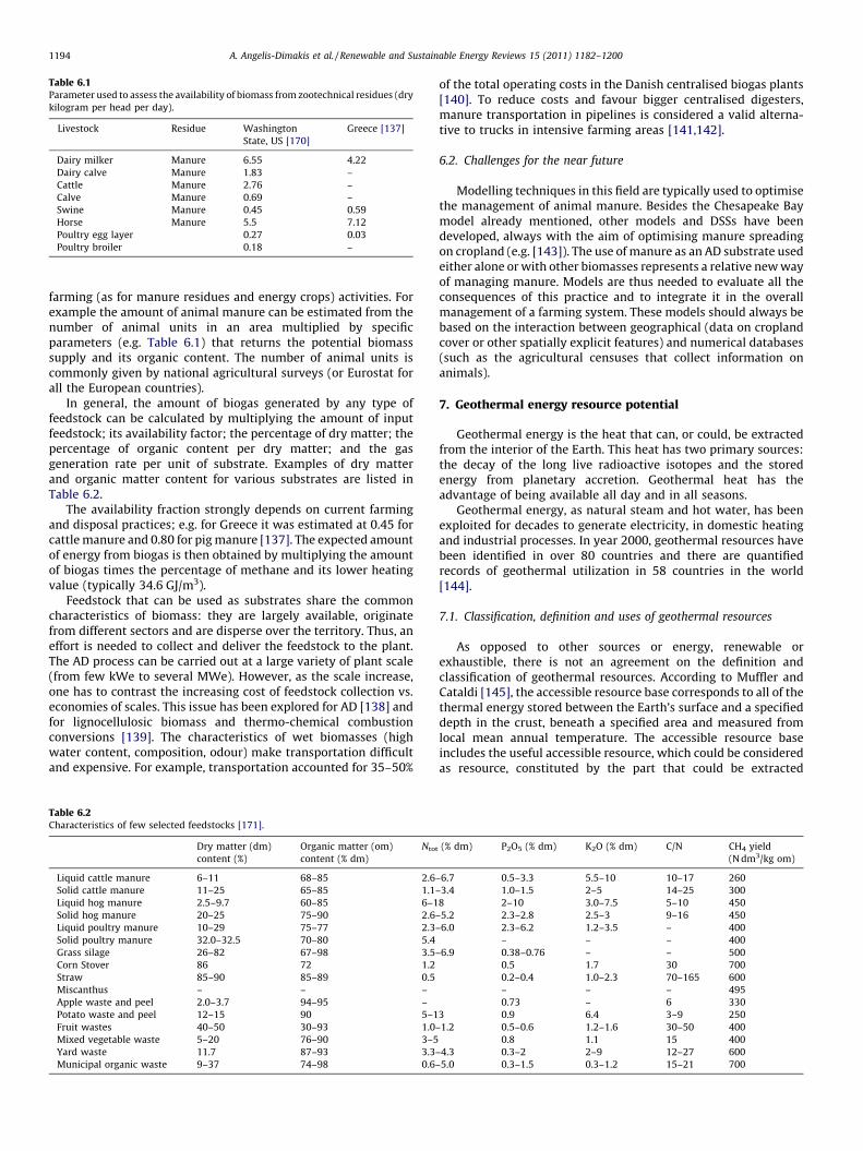
Table 6.1Parameter used to assess the availability of biomass from zootechnical residues (dry

kilogram per head per day).

Livestock Residue Washington

State, US [170]

Greece [137]

Dairy milker Manure 6.55 4.22

Dairy calve Manure 1.83 –

Cattle Manure 2.76 –

Calve Manure 0.69 –

Swine Manure 0.45 0.59

Horse Manure 5.5 7.12

Poultry egg layer 0.27 0.03

Poultry broiler 0.18 –


farming (as for manure residues and energy crops) activities. Forexample the amount of animal manure can be estimated from thenumber of animal units in an area multiplied by specificparameters (e.g. Table 6.1) that returns the potential biomasssupply and its organic content. The number of animal units iscommonly given by national agricultural surveys (or Eurostat forall the European countries).

In general, the amount of biogas generated by any type offeedstock can be calculated by multiplying the amount of inputfeedstock; its availability factor; the percentage of dry matter; thepercentage of organic content per dry matter; and the gasgeneration rate per unit of substrate. Examples of dry matterand organic matter content for various substrates are listed inTable 6.2.

The availability fraction strongly depends on current farmingand disposal practices; e.g. for Greece it was estimated at 0.45 forcattle manure and 0.80 for pig manure [137]. The expected amountof energy from biogas is then obtained by multiplying the amountof biogas times the percentage of methane and its lower heatingvalue (typically 34.6 GJ/m3).

Feedstock that can be used as substrates share the commoncharacteristics of biomass: they are largely available, originatefrom different sectors and are disperse over the territory. Thus, aneffort is needed to collect and deliver the feedstock to the plant.The AD process can be carried out at a large variety of plant scale(from few kWe to several MWe). However, as the scale increase,one has to contrast the increasing cost of feedstock collection vs.economies of scales. This issue has been explored for AD [138] andfor lignocellulosic biomass and thermo-chemical combustionconversions [139]. The characteristics of wet biomasses (highwater content, composition, odour) make transportation difficultand expensive. For example, transportation accounted for 35–50%

Table 6.2Characteristics of few selected feedstocks [171].

Dry matter (dm)

content (%)

Organic matter (om)

content (% dm)

Ntot

Liquid cattle manure 6–11 68–85 2.6–

Solid cattle manure 11–25 65–85 1.1–

Liquid hog manure 2.5–9.7 60–85 6–1

Solid hog manure 20–25 75–90 2.6–

Liquid poultry manure 10–29 75–77 2.3–

Solid poultry manure 32.0–32.5 70–80 5.4

Grass silage 26–82 67–98 3.5–

Corn Stover 86 72 1.2

Straw 85–90 85–89 0.5

Miscanthus – – –

Apple waste and peel 2.0–3.7 94–95 –

Potato waste and peel 12–15 90 5–1

Fruit wastes 40–50 30–93 1.0–

Mixed vegetable waste 5–20 76–90 3–5

Yard waste 11.7 87–93 3.3–

Municipal organic waste 9–37 74–98 0.6–

of the total operating costs in the Danish centralised biogas plants[140]. To reduce costs and favour bigger centralised digesters,manure transportation in pipelines is considered a valid alterna-tive to trucks in intensive farming areas [141,142].


Modelling techniques in this field are typically used to optimisethe management of animal manure. Besides the Chesapeake Baymodel already mentioned, other models and DSSs have beendeveloped, always with the aim of optimising manure spreadingon cropland (e.g. [143]). The use of manure as an AD substrate usedeither alone or with other biomasses represents a relative new wayof managing manure. Models are thus needed to evaluate all theconsequences of this practice and to integrate it in the overallmanagement of a farming system. These models should always bebased on the interaction between geographical (data on croplandcover or other spatially explicit features) and numerical databases(such as the agricultural censuses that collect information onanimals).

7. Geothermal energy resource potential

Geothermal energy is the heat that can, or could, be extractedfrom the interior of the Earth. This heat has two primary sources:the decay of the long live radioactive isotopes and the storedenergy from planetary accretion. Geothermal heat has theadvantage of being available all day and in all seasons.

Geothermal energy, as natural steam and hot water, has beenexploited for decades to generate electricity, in domestic heatingand industrial processes. In year 2000, geothermal resources havebeen identified in over 80 countries and there are quantifiedrecords of geothermal utilization in 58 countries in the world[144].

7.1. Classification, definition and uses of geothermal resources

As opposed to other sources or energy, renewable orexhaustible, there is not an agreement on the definition andclassification of geothermal resources. According to Muffler andCataldi [145], the accessible resource base corresponds to all of thethermal energy stored between the Earth’s surface and a specifieddepth in the crust, beneath a specified area and measured fromlocal mean annual temperature. The accessible resource baseincludes the useful accessible resource, which could be consideredas resource, constituted by the part that could be extracted

(% dm) P2O5 (% dm) K2O (% dm) C/N CH4 yield

(N dm3/kg om)

6.7 0.5–3.3 5.5–10 10–17 260

3.4 1.0–1.5 2–5 14–25 300

8 2–10 3.0–7.5 5–10 450

5.2 2.3–2.8 2.5–3 9–16 450

6.0 2.3–6.2 1.2–3.5 – 400

– – – 400

6.9 0.38–0.76 – – 500

0.5 1.7 30 700

0.2–0.4 1.0–2.3 70–165 600

– – – 495

0.73 – 6 330

3 0.9 6.4 3–9 250

1.2 0.5–0.6 1.2–1.6 30–50 400

0.8 1.1 15 400

4.3 0.3–2 2–9 12–27 600

5.0 0.3–1.5 0.3–1.2 15–21 700


economically and legally at some specified time in the future (lessthan a hundred years). Fig. 7.1, taken from Muffler and Cataldi[145], illustrates in graphic form these and other terms that may beused within the context of geothermal resource assessment.

There is another common criterion based on the enthalpy of thegeothermal fluids. The enthalpy could be considered almostproportional to temperature, so the resources are divided intolow, medium and high enthalpy; but there is no general agreementon the arbitrary temperature ranges used. Another frequentdistinction is made between liquid dominated geothermal systemsand vapor dominated systems.

Geothermal energy can be used for direct application, with awide variety of end uses such as heating and cooling, industry,greenhouses, fish farming, and health spas [144]. While electricityproduction requires high temperature geothermal resources (over100–150 8C) and implies drilling and pumping water from depth,direct application can use both high and low temperaturegeothermal resources and is therefore much more widespreadin the world than electricity production. Indeed, the almostconstant temperature of the soil few meters under the surfacealmost everywhere, can serve as a perfect heat source for small andsimple heating and/or cooling systems driven by heat pumps.

In general, an assessment procedure should be used todetermine the amount and the form of geothermal energy storedin the subsurface and these factors would restrict the type ofapplication and extraction method [146].

Usually, the exploration program is developed on a step by stepbasis, closely following those of traditional fossil fuels search andexploitation. The initial phase is based on the selection of the mostpromising areas. The surface investigations in the selected areaform the pre-feasibility phase, while the subsequent feasibilityphase consists of deep exploratory drilling and reservoir testing. Atan early stage in exploration, prior to drilling, resource assessmentis largely qualitative. Once a few wells have been drilled, it will bepossible to undertake a more accurate resource assessment. The
[()TD$FIG]
Fig. 7.1. Diagram representing the different categories of geothermal resources

according to Muffler and Cataldi [145].

final phases of the project are those of development andexploitation. During each stage of the process, the least interestingareas are gradually eliminated so that efforts are concentrated onthe remaining, more promising ones.

A general approach to both targeting a geothermal well locationand assessing resource capacity is to gather data about anomalies,and to define a conceptual model consistent with the availableinformation.

7.2. Geothermal exploration data

Once a geothermal region has been identified, variousexploration techniques are used to locate the most interestingareas. These techniques are based on several surveys which collectdata to estimate temperature, reservoir volume and permeabilityat various depths, as well as to predict whether wells will producesteam or just hot water [147].

Geological and hydrogeological studies provide basic informa-tion to define any exploration program. The presence anddistribution of young volcanic rocks, active volcanoes, craters,calderas, faults and fractures are the main data used in the earlystages of geothermal resource assessment, aiming to identifygeothermal phenomena and to estimate the size of the resource.Geochemical surveys are a useful means of determining whetherthe geothermal source is water or vapor dominated. The chemicalcharacteristics of the deep fluid can be interpreted as geotherm-ometers, i.e. a set of experimental relations that allow to define themodel of the reservoir and its physical characteristics, such astemperature, electrical conductivity, density, etc., starting from themeasured concentration of some minerals. Other commonly usedtechniques to infer the temperature of the fluids are: direct currentresistivity, transient electromagnetic (TEM), and magneto-telluric(MT) studies [148].

7.3. Data integration for targeting promising areas and well sites

The decision making process involved in locating prospectiveareas, recommended for further study or exploratory drilling,demands to combine, integrate and interpret the results ofgeological, geochemical, geophysical and other surveys [149].GIS models have been successfully used in performing these tasks.They can be grouped according to their main goal: selectingpromising geothermal fields for further exploration at regionalscale or defining specific sites for well drilling at local/basin scale.

The methodologies used by Noorollahi et al. [150] and byYousefi et al. [151] are quite similar and belong to the first group ofstudies. The datasets used in the analysis consist of geological,geochemical and geophysical information. Boolean integrationmethod by using ‘‘or’’ and ‘‘and’’ operators were applied tocombine all the evidence layers within each type of information,resulting in three suitability maps: geological, geochemical andgeophysical (thermal). The final geothermal favourability map isthen created by weighted overlay. Noorollahi et al. [150] alsopresents a distance relationship analysis to determine thepredominant distance between actual geothermal wells andinteresting geological features (such as faults or hot springs)represented in a GIS layer. The results are buffers around thoseknown features that can be combined to obtain the final favorabilitymap. Carranza et al. [152] focuses on the analysis of spatialdistribution of geothermal prospects and thermal springs (evi-dences), and their spatial association with geological features(resources), highlighting their strong positive correlation. As a result,the mapping of high geothermal potential is presented.The methodology presented by Blewitt [174] also studies spatialrelationships at regional scale, but between geologic structures andregional tectonic strain measured with GPS geodetic observations.

Table 7.1Overview of estimated geothermal resources potential in the world [156].

Lower limit for the potential

of geothermal resources

World geothermal potential

for identified resources

Upper limit for total world

geothermal potential

Resources suitable for electricity generation 0.05 TWe 0.2 TWe 1–2 TWe

Resources only suitable for direct use 1 TWth 4.4 TWth 22–44 TWth

Total potential 1.5 TWth 6 TWth 30–60 TWth


The final stage of a feasibility study is exploratory well drilling,and this is the only means of determining the real characteristics ofthe existing resource and thus assessing its potential. Several studiesat local/basin scales have used GIS for the siting of exploratory wellsin the most favorable areas. In the case reported by Prol-Ledesma[153], three knowledge driven models are proposed: Boolean logicmodel, index overlay model and fuzzy data analysis. In all models thesame input data are used and the same conditions need to besatisfied. The Boolean method proved to be more restrictive andtherefore more dependable for exploration well siting. Noorollahiet al. [149] introduce the results of an environmental suitabilityanalysis (e.g. land cover, residential areas, etc.) to select the mostpromising well sites. As stated by Cumming [154], using aconceptual model approach in well targeting has the advantage oftesting the properties of the model, especially for temperatures.

7.4. Resource conceptual model

Geothermal conceptual models bring together the observed andinferred information that best illustrates the reservoir fluid androck properties. According to the volume method [145], the electricpower generation potential from an identified geothermal systemdepends on the thermal energy in the reservoir, the amount ofthermal energy that can be extracted from the reservoir at thewellhead, and the efficiency with which that wellhead thermalenergy can be converted to electric power. The volume methodwas quickly established as the standard approach and most of theassessments made in parts of the United States rely on a version ofthis method. Nowadays, a new assessment of identified geother-mal resources is being carried out by the U.S. Geological Survey,still using the volume method while incorporating some modifica-tions regarding, among others, the temperature and depth rangesfor electrical power production. For example, the assumed 150 8Clower limit for electric power production is under revision toinclude power production from moderate temperature systemsusing binary technology [155].

A more accurate assessment method is the use of geothermalsimulation models to estimate the generation capacity of a givengeothermal field. A detailed knowledge on the internal conditionsof the geothermal reservoir is needed, and therefore, this methodcan hardly be applied until several wells have been drilled [156].

7.5. Geothermal resource assessments and maps

Stefansson [156] recently presented an estimation of thegeothermal potential of the world. The volumetric assessmentmethod on the identified resources was assumed to provide themost likely value, while the hidden resources were assumed to be5–10 times than those identified and the results obtained bysimulation models tended to be 4–5 times lower than the firstmethod. The results are summarized in Table 7.1.

The geothermal resources of most European countries havebeen estimated and compiled in an atlas [146]. A volumetric heatcontent model was the basis for calculating the resources,assuming that exploitation would take place in a doublet system.Mapping of geothermal potential at regional scale have beenimplemented using GIS in many other countries ([157–159]).


The utilization of geothermal energy has been limited to areasin which geological conditions allow a carrier liquid or steam totransfer the heat from deep zones, but only a small fraction of thegeothermal potential has been developed so far, and there is amplespace for an increased use of geothermal energy both for electricitygeneration and direct applications.

Most current studies on the classification of favorable areashave been based on GIS tools. However, technical improvementsand innovative technologies, such as enhanced geothermalsystems (EGS) and binary plants, offer new perspectives in thissector. EGS technology is based on developing new reservoirsthrough the creation and stimulation of fractures and thus itrequires existing models of thermal energy recovery factors andresource assessment tools to be adapted. In addition, advances inpower production technology and the scientific understanding ofgeothermal systems indicate that some important elements ofgeothermal assessment methodology require detailed examina-tion and revision, which indeed makes the updating of geothermalassessment appraisals obligatory.

8. Conclusion

A survey of methods and tools to evaluate the availability ofrenewable resources (i.e., solar, wind, wave, biomass andgeothermal energy) has been presented. In particular, potential,theoretical and exploitable energy have been differentiated andinvestigated for each kind of resource. All these energy sourcesshare the feature of being distributed over the territory and ofbeing measurable only at specific sites. This means that they allneed tools to determine their spatial dimension and these may beprovided by geostatistical tools or by remote sensed spatialinformation. In quite the same way, they all require GISs both toprocess data and to demonstrate their local impacts. Indeed, theirpresence on the territory generates some form of conflict withother uses, from the subtraction of land otherwise dedicated tofood agriculture (as it happened in Mexico in 2007 with the famous‘‘tortilla riot’’) or by perturbing existing landscapes (as claimed byvarious associations in UK). To correctly support decisions onrenewable energy sources, studies should thus deepen the evalua-tion of these conflicts and take into account not just the exercise ofthe energy conversion plants, but their entire life-cycle. TheUniversity of Sydney’s Integrated Sustainability Analysis report(see [160]), for instance, estimates at something between 20 and40 kg CO2eq/MWh, depending on the estimated life and capacityfactor, the GHG emission due to the building, operating anddecommissioning of wind turbines. ‘‘Renewable’’ does not mean‘‘completely CO2 neutral’’ and thus more detailed and comprehen-sive analysis tools will probably be developed in the near future.

An additional important issue (that has not been highlighted inthe previous sections) is that none of the renewable sourceanalysed would be able to supply the growing energy need of evensmall isolated areas of the world. It is thus necessary to integratefew of them and choose the best mix of different resources. Theobjective of choosing a mix of plants that maximizes environmen-tal sustainability as well as economic viability can somehow be


conflicting with the maximization of the energy supply reliability.Methods and tools that deal with the this type of integration arealready present in the literature. An example is HOMER computermodel [161,162]: it is an easy to use tool that simplifies the task ofevaluating design options for both off grid and grid connectedrenewable power systems for remote, stand alone, and distributedgeneration applications (https://analysis.nrel.gov/homer/). It com-prises three different modules:

� a simulation module, at hourly time scale, that compares theelectrical and thermal demand to the energy that a mixedrenewable/fossil system can supply, and estimates the cost ofinstalling and operating the system over the lifetime of theproject. HOMER simulates system configurations with severaldifferent combinations of components, and discards all thosethat do not respect reliability or cost constraints;� an optimization module: after simulating all the possible system

configurations, HOMER orders feasible configurations from themost to the least cost effective, so that different design optionscan be compared;� a sensitivity analysis module: that repeats optimization for

different values of parameters to take into account uncertainties.

HOMER can thus find feasible solutions to design an efficientmix of renewable energy plants on the basis of a cost criterion. Itcould be easily expanded to consider other objectives such as landoccupation or GHG reduction. Yet another research direction willemerge as extremely important in the near future: the manage-ment and control of a mix of existing plants, subject to anintermittent resource availability, that has to meet the fluctuatingenergy demands and be embedded into an energy network,particularly for electricity, that was originally conceived with acentralized structure. The energy flow may in fact reverse from thenodes to the center of the network and this may create toughproblems to current devices. A large restructuring of the energynetworks will probably be necessary in the future and this willentail the consideration of multiple objectives and multiplecriteria, including the competition for land use. Examples relatedto design and planning decision problems, solved throughmathematical programming and multicriteria approaches, canalready be found in the literature at local scale (for example: [163–165]), but more flexible and integrated tools that coupleenvironmental and decision models, databases and assessmenttools, integrated under a GIS based Graphical User Interface (GUI)[166–168] are still necessary to implement EnvironmentalDecision Support Systems that can operate on different territoriesand multiple scales to plan and manage an efficient mix ofrenewable energy sources.

References

[1] Suri M, Huld TA, Dunlop ED, Ossenbrink HA. Potential of solar electricitygeneration in the European Union member states and candidate countries.Solar Energy 2007;81:1295–305.

[2] Suri M, Hofierka J. A new GIS-based solar radiation model and its applicationto photovoltaic assessments. Transactions in GIS 2004;8(2):175–90.

[3] Biberacher M, Gadocha S, Zocher D. GIS based model to optimize possible selfsustaining regions in the context of a renewable energy supply. In: Proceed-ings of the iEMSs fourth biennial meeting: international congress on envi-ronmental modelling and software; 2008.

[4] Greenpeace/EREC European Renewable Energy Council. Energy [r]evolution –a sustainable global energy outlook; 2008.

[5] Hoogwijk M. On the global and regional potential of renewable energysources. Utrecht University; 2004 , http://www.library.uu.nl/digiarchief/dip/diss/2004-0309-123617/full.pdf.

[6] Sørensen B. GIS management of solar resource data. Solar Energy Materials &Solar Cells 2001;67:503–9.

[7] Suri M. Solar resource data and tools for an assessment of photovoltaicsystems. In: Jager-Waldau A, editor. Status report 2006. Luxembourg: Officefor Official Publications of the European Communities; 2006. p. 96–102.

[8] Meteotest. Meteonorm version 6.1 – handbook; 2008, www.meteonorm. com.[9] Hammer A, Heinemann D, Hoyer C, Kuhlemann R, Lorenz E, Muller R, et al.

Solar energy assessment using remote sensing technologies. Remote Sensingof Environment 2003;86(3):423–32.

[10] Muller RW, Beyer HG, Cors S, Dagestad KF, Dumortier D, Ineichen P, et al. Theuse of MSG data within a new type of solar irradiance calculation scheme. In:Proceedings of the 2002 EUMETSAT meteorological satellite conference;2002.p. 608.

[11] Suri M, Redmund J, Cebecauer T, Dumotier D, Wald L, Huld T, et al. First stepsin the cross-comparison of solar resource spatial products in Europe. In:Proceeding of the EUROSUN 2008, 1st international conference on solarheating, cooling and buildings; 2008.

[12] Rigollier C, Lefevre M, Wald L. The method Heliosat-2 for deriving shortwavesolar radiation from satellite images. Solar Energy 2004;77:159–69.

[13] Cano D, Monget JM, Albuisson M, Guillard H, Regas N, Wald L. A method forthe determination of the global solar radiation from meteorological satellitedata. Solar Energy 1986;37(1):31–9.

[14] Betcke J, Kuhlemann R, Hammer A, Drews A, Lorenz E, Girodo M, et al. Finalreport of the Heliosat-3 project, Oldenburg; 2006 [online] http://www.heliosat3.de/.

[15] Huld T, Suri M, Dunlop E. A GIS-based system for performance assessment ofsolar energy systems over large geographical regions. In: Proceedings of thesolar 2006 conference; 2006.

[16] Cebecauer T, Huld T, Suri M. High-resolution digital elevation model forimproved PV yield estimates. In: Proceedings of the 22nd European photo-voltaic solar energy conference; 2007.

[17] Cros S, Albuisson M, Lefevre M, Rigollier C, Wald L. HelioClim: a long-termdatabase on solar radiation for Europe and Africa. In: Proceedings of the 14thEuroSun2004 conference; 2004. p. 916–20.

[18] HelioClim online; 2008. www.helioclim.net.[19] Biberacher M, Gadocha S, Zocher D. Implementation of a GEOdatabase to

administrate global energy resources. In: Proceedings of the iEMSs fourthbiennial meeting: international congress on environmental modelling andsoftware; 2008.

[20] Kassner R, Koppe W, Schuttenberg T, Bareth G. Analysis of the solar potentialof roofs by using official LIDAR data. In: Proceedings of the internationalsociety for photogrammetry and remote sensing XXIth congress; 2008.

[21] Muller M, Surmann H, Pervolz K, May S. The accuracy of 6D SLAM using theAIS 3D laser scanner. In: IEEE international conference on multisensor fusionand integration for intelligent systems; 2006.

[22] Danish Wind Industry Association. A wind energy pioneer: Charles F. Brush.www.talentfactory.dk/en/pictures/brush.htm. Retrieved on 8 October 2010.

[23] World Wind Energy Association. World wind energy report 2008; www.wwindea.org/home/images/stories/worldwindenergyreport2008_s.pdf.Retrieved on 16 March 2009.

[24] Lalas DP. Wind energy estimation and siting in complex terrain. InternationalJournal of Sustainable Energy 1985;3(2):43–71.

[25] Nfaoui H, Buret J, Sayigh AAM. Wind characteristics and wind energy poten-tial in Morocco. Solar Energy 1998;63:51–60.

[26] Frandsen S, Christensen CJ. Accuracy of estimation of energy production fromwind power plants. Wind Engineering 1992;16(5):257–67.

[27] Alawaji SH. Wind energy resource assessment in Saudi Arabia-I, networkdesign and description. Renewable Energy 1996;7:319–28.

[28] Landberg L, Myllerup L, Rathmann O, Lundtang Petersen E, Hoffmann Jør-gensen B, Badger J, et al. Wind resource estimation – an overview. WindEnergy 2003;6:261–71.

[29] Choisnard J, Lafrance G, Bernier M. SAR-satellite for offshore and coastal windresource analysis, with examples from St. Lawrence Gulf, Canada. WindEngineering 2004;28(4):367–82.

[30] Bruun Christiansen M, Koch W, Horstmann J, Bay Hasager C, Nielsen M. Windresource assessment from C-band SAR. Remote Sensing of Environment2006;105(1):68–81.

[31] Lackner MA, Rogers AL, Manwell JF. The round robin site assessment method:a new approach to wind energy site assessment. Renewable Energy2008;33:2019–26.

[32] Carta JA, Ramırez P, Velazquez S. A review of wind speed probability dis-tributions used in wind energy analysis case studies in the Canary Islands.Renewable and Sustainable Energy Reviews 2009;13(5):933–55.

[33] Stevens MJM, Smulders PT. The estimation of the parameters of the Weibullwind speed distribution for wind energy utilization purposes. Wind Engi-neering 1979;3(2):132–45.

[34] Sen Z, Sahin AD. Regional assessment of wind power in western Turkeyby the cumulative semivariogram method. Renewable Energy 1997;12:169–77.

[35] Rogers AL, Rogers JW. Comparison of the performance of four measure–correlate–predict algorithms. Journal of Wind Engineering and IndustrialAerodynamics 2005;93:243–64.

[36] Addison JF, Hunter A, Bass J, Rebbeck M. A neural network version of theMeasure–Correlate–Predict algorithm for estimating wind energy yield. In:Proceedings of the international congress and exhibition on condition moni-toring and diagnostic management; 2000.

[37] Bechrakis DA, Deane JP, McKeogh EJ. Wind resource assessment of an areausing short term data correlated to a long term data set. Solar Energy2004;76(6):725–32.

[38] Ayotte K. Computational modelling for wind energy assessment. Journal ofWind Engineering and Industrial Aerodynamics 2008;96:1571–90.

https://analysis.nrel.gov/homer/

http://www.library.uu.nl/digiarchief/dip/diss/2004-0309-123617/full.pdf

http://www.library.uu.nl/digiarchief/dip/diss/2004-0309-123617/full.pdf

http://www.meteonorm.com/

http://www.heliosat3.de/

http://www.heliosat3.de/


http://www.talentfactory.dk/en/pictures/brush.htm

http://www.wwindea.org/home/images/stories/worldwindenergyreport2008_s.pdf




[39] Troen I, Petersen EL. The European Wind Atlas. Denmark: Risø NationalLaboratories; 1989, 656 pp..

[40] Taylor PA, Walmsley JL, Salmon JR. A simple model of neutrally stratifiedboundary-layer flow over real terrain incorporating wave number-depen-dent scaling. Boundary-Layer Meteorology 1983;26:169–89.

[41] Bowen AJ, Mortensen NG. WAsP prediction errors due to site orography.Technical report Risø-R-995(EN). Roskilde, Denmark: Risø National Labora-tories; 2004.

[42] Palma JMLM, Castro FA, Ribeiro LF, Rodrigues AH, Pinto AP. Linear andnonlinear models in wind resource assessment and wind turbine micro-siting in complex terrain. Journal of Wind Engineering and Industrial Aero-dynamics 2008;96:2308–26.

[43] Lyons TJ, Bell MJ. Mesoscale variations in available wind power potential.Solar Energy 1990;45:149–66.

[44] Katsoulis BD, Metaxas DA. The wind energy potential of western Greece. SolarEnergy 1992;49(6):463–76.

[45] Frank HP, Landberg L. Modelling the wind climate of Ireland. Boundary-LayerMeteorology 1997;85:359–78.

[46] Brower M, Zack JW, Bailey B, Schwartz MN, Elliott DL. Mesoscale modelling asa tool for wind resource assessment and mapping. In: Proceedings of the 14thconference on applied climatology; 2004.

[47] Pepper DW, Wang X. Application of an h-adaptive finite element modelfor wind energy assessment in Nevada. Renewable Energy 2007;32:1705–22.

[48] Kondo H, Tokairin T, Kikegawa Y. Calculation of wind in a Tokyo urban areawith a mesoscale model including a multi-layer urban canopy model. Journalof Wind Engineering and Industrial Aerodynamics 2008;96(10–11):1655–66.

[49] Voivontas D, Assimacopoulos D, Mourelatos A, Corominas J. Evaluation ofrenewable energy potential using a GIS decision support system. RenewableEnergy 1998;13(3):333–44.

[50] Acker TL, Williams SK, Duque E, Brummels G, Buechler J. Wind resourceassessment in the state of Arizona: inventory, capacity factor, and cost.Renewable Energy 2007;32:1453–66.

[51] Hoogwijk M, de Vries B, Turkenburgm W. Assessment of the global andregional geographical, technical and economic potential of onshore windenergy. Energy Economics 2004;26(5):889–919.

[52] de Vries B, van Vuuren D, Hoogwijk M. Renewable energy sources: theirglobal potential for the first-half of the 21st century at a global level: anintegrated approach. Energy Policy 2007;35:2590–610.

[53] Petersen EL.In: State of the art and challenges in wind power meteorologyFVS workshop; 2006.

[54] Dhanju A, Whitaker P, Kempton W. Assessing offshore wind resources: anaccessible methodology. Renewable Energy 2008;33(1):55–64.

[55] Lange B, Højstrup J. Evaluation of the wind-resource estimation programWAsP for offshore applications. Journal of Wind Engineering and IndustrialAerodynamics 2001;89:271–91.

[56] Lange B, Larsen S, Højstrup J, Barthelmie R. The influence of thermal effects onthe wind speed profile of the coastal marine boundary layer. Boundary-LayerMeteorology 2004;112:587–617.

[57] World Energy Council. Survey of energy resources; 2007, London.[58] Krogstad HE, Barstow SF. Satellite wave measurements for coastal engineer-

ing applications. Coastal Engineering 1999;37(3–4):283–307.[59] Barstow SF, Haug O, Krogstad HE. Satellite altimeter data in wave energy

studies. In: Proceedings of the 3rd international symposium on ocean wavemeasurement and analysis (Waves 97); 1998.

[60] Smith GH, Venugopal V, Wolfram J. Wave period group statistics for real seawaves and wave energy extraction. In: Proceedings of the institution ofmechanical engineers, Part M. Journal of Engineering for the MaritimeEnvironment 2006;99–115.

[61] Rusu E, Guedes Soares C. Numerical modelling to estimate the spatialdistribution of the wave energy in the Portuguese nearshore. RenewableEnergy 2009;34:1501–16.

[62] Folley M, Whittaker TJT. Analysis of the nearshore wave energy resource.Renewable Energy 2009;34(7):1709–15.

[63] ESBI Environmental Services. Accessible wave energy resource atlas, Ireland:2005. Marine Institute/Sustainable Energy Ireland; 2005.

[64] ABP Marine Environmental Research Limited. Atlas of UK marine renewableenergy resources: technical report; 2008, Available at SSRN: http://www.abpmer.co.uk/.

[65] Pontes MT, Aguiar R, Oliveira Pires H. A nearshore wave energy atlas forPortugal. Journal of Offshore Mechanics and Arctic Engineering 2005;127:249–55.

[66] Wilson JH, Beyene A. California wave energy resource evaluation. Journal ofCoastal Research 2007;23(3):679–90.

[67] Dunnett D, Wallace JS. Electricity generation from wave power in Canada.Renewable Energy 2009;34(1):179–95.

[68] Henfridsson U, Neimane V, Strand K, Kapper R, Bernhoff H, Danielsson O, et al.Wave energy potential in the Baltic Sea and the Danish part of the NorthSea, with reflections on the Skagerrak. Renewable Energy 2007;32(12):2069–84.

[69] Boehme T, Taylor J, Wallace R, Bialek J. Matching renewable electricitygeneration with demand: full report. Institute for Energy Systems, Universityof Edinburgh; 2006.

[70] Nobre A, Pacheco M, Jorge R, Lopes MFP, Gato LMC. Geo-spatial multi-criteriaanalysis for wave energy conversion system deployment. Renewable Energy2009;34:97–111.

[71] Prest R, Daniella T, Ostendorf B. Using GIS to evaluate the impact of exclusionzones on the connection cost of wave energy to the electricity grid. EnergyPolicy 2007;35:4516–28.

[72] Graham SB, Wallace AR, Connor G. Geographical information system (GIS)techniques applied to network integration of marine energy. In: Proceedingsof the universities power engineering conference, vol. 38; 2003.

[73] Mueller M, Wallace R. Enabling science and technology for marine renewableenergy. Energy Policy Foresight Sustainable Energy Management and theBuilt Environment Project 2008;36(12):4376–82.

[74] Harrison GP, Wallace AR. Climate sensitivity of marine energy. RenewableEnergy 2005;30(12):1801–17.

[75] Brown S. Measuring carbon in forests: current status and future challenges.Environmental Pollution 2002;116(3):363–72.

[76] Brown S. Estimating biomass and biomass change in tropical forests: aprimer. FAO Forestry Paper 134. Rome, Italy: Food and Agriculture Organi-zation; 1997.

[77] Jenkins JC, Chojnacky DC, Heath LS, Birdsey RA. National-scale biomassestimators for United States tree species. Forest Science 2003;49:12–35.

[78] Zianis D, Muukkonen P, Makipaand R, Mencuccini M. Silva Fennica. Mono-graphs 4: biomass and stem volume equations for tree species in Europe. TheFinnish Society of Forest Science, The Finnish Forest Research Institute; 2005.

[79] Brown SL, Schroeder P, Kern JS. Spatial distribution of biomass inforests of the eastern USA. Forest Ecology and Management 1999;123(1):81–90.

[80] Joosten R, Schumacher J, Wirth C, Schulte A. Evaluating tree carbon predic-tions for beech (Fagus sylvatica L.) in Western Germany. Forest Ecology andManagement 2004;189:87–96.

[81] Lehtonen A, Makipaa R, Heikkinen J, Sievanen R, Liski J. Biomass expansionfactors (BEFs) for Scots pine, Norway spruce and birch according to stand agefor boreal forests. Forest Ecology and Management 2004;188:211–24.

[82] Jalkanen R, Makipaa G, Stahl A, Lehtonen H, Petersson. Estimation of thebiomass stock of trees in Sweden: comparison of biomass equations and age-dependent biomass expansion factors. Annals of Forest Science 2005;62(8):845–51.

[83] Esteban Pascual LE. Modulo: Biomasa residual seca y cultivos energeticos.Fuentes y evaluacion de recursos. Apuntes CEDER-CIEMAT; 2005.

[84] Panichelli L, Gnansounou E. GIS modelling of forest wood residues potentialfor energy use based on forest inventory data: methodological approach andcase study application. In: Sanchez-Marre M, Bejar J, Comas J, Rizzoli A,Guariso G, editors. Proceedings of the iEMSs fourth biennial meeting: inter-national congress on environmental modelling and software (iEMSs 2008).2008. p. 1239–46.

[85] Panichelli L, Gnansounou E. GIS-based approach for defining bioenergyfacilities location: a case study in Northern Spain based on marginal deliverycosts and resources competition between facilities. Biomass and Bioenergy2008;32:289–300.

[86] von Gadow K, Hui G. Modelling forest development. Springer: Kluwer Aca-demic Publishers; 2001.

[87] Hasenauer H. In: Hasenauer H, editor. Sustainable forest management:growth models for Europe. Springer; 2006.

[88] Umeki K, Lim E-M, Honjo T. A GIS-based simulation program to predict multi-species size-structure dynamics for natural forests in Hokkaido, northernJapan. Ecological Informatics 2008;3:218–27.

[89] Masera OR, Garza-Caligaris JF, Kanninen M, Karjalainen T, Liski J, Nabuurs GJ,et al. Modeling carbon sequestration in afforestation, agroforestry and forestmanagement projects: the CO2FIX V.2 approach. Ecological Modelling2003;164:177–99.

[90] Schelhaas MJ, van Esch PW, Groen TA, de Jong BHJ, Kanninen M, Liski J, et al.CO2FIX V 3.1 – description of a model for quantifying carbon sequestration inforest ecosystems and wood products. ALTERRA Report 1068; 2004, Wagen-ingen, The Netherlands.

[91] Koopmans A, Koppejan J. Generation, utilization and availability of agricul-tural and forest residues. In: Proceedings of the regional expert consultationon modern applications of biomass energy; 1997.

[92] Lewandowski I, Weger J, van Hooijdonk A, Havlickova K, van Dam J, Faaij A.The potential biomass for energy production in the Czech Republic. Biomassand Bioenergy 2006;30:405–21.

[93] Perlack RD, Wright LL, Turhollow AF, Graham RL, Stokes BJ, Erbach DC. USABiomass as Feedstock for a Bioenergy and Bioproducts Industry: the technicalfeasibility of a billion-ton annual supply. U.S. Department of Energy & U.S.Department of Agriculture; 2005, Available at: http://feedstockreview.ornl.gov/pdf/billion_ton_vision.pdf.

[94] Bhattacharya SC, Salam PA, Runqing H, Somashekar HI, Racelis DA, RathnasiriPG, et al. An assessment of the potential for non-plantation biomass resourcesin selected Asian countries for 2010. Biomass and Bioenergy 2005;29(3):153–66.

[95] Dalianis C, Panoutsou C. Energy potential of agricultural residues in EU.EUREC Network on Biomass (Bioelectricity). Final report. Contract no: RENACT 94-0053; 1995.

[96] Sokhansanj S, Turhollow AF. Baseline cost for corns Stover collection. AppliedEngineering in Agriculture 2002;18(5):525–30.

[97] Graham RL, Nelson R, Sheehan J, Perlack RD, Wright LL. Current and potentialU.S. Corn Stover supplies. Agronomy Journal 2007;99:1–11.

[98] Aylott MJ, Casella E, Tubby I, Street NR, Smith P, Taylor G. Yield and spatialsupply of bioenergy poplar and willow short-rotation coppice in the UK. NewPhytologist 2008;178(2):358–70.

http://www.abpmer.co.uk/

http://www.abpmer.co.uk/

http://feedstockreview.ornl.gov/pdf/billion_ton_vision.pdf

http://feedstockreview.ornl.gov/pdf/billion_ton_vision.pdf


[99] Fischer G, Prieler S, van Velthuizen H. Biomass potentials of miscanthus,willow and poplar: results and policy implications for Eastern Europe,Northern and Central Asia. Biomass and Bioenergy 2005;28(2):119–32.

[100] Field CB, Campbell JE, Lobell DB. Biomass energy: the scale of the potentialresource. Trends in Ecology and Evolution 2008;23(2):65–72.

[101] Fiorese G, Guariso G. A GIS-based approach to evaluate biomass potentialfrom energy crops at regional scale. Environmental Modelling & Software2010;25(6):702–11.

[102] McLaughlin SB, de la Torre Ugarte DG, Garten CT, Lynd LR, Sanderson MA,Tolbert VR, et al. High-value renewable energy from prairie grasses. Envi-ronmental Science & Technology 2002;36(10):2122–9.

[103] Graham RL, Liu W, Jager HI, English BC, Noon CE, Daly MJ. A regional-scaleGIS-based modelling system for evaluating the potential costs and supplies ofbiomass from biomass crops. In: Proceedings of the 7th national bioenergyconference BIOENERGY; 1996.

[104] Graham RL, English BC, Noon CE. A geographic information system-basedmodelling system for evaluating the cost of delivered energy crop feedstock.Biomass and Bioenergy 2000;18(4):309–29.

[105] Labrecque S, Fournier RA, Luther JE, Piercey D. A comparison of four methodsto map biomass from Landsat-TM and inventory data in western Newfound-land. Forest Ecology and Management 2006;226:129–44.

[106] Remmel TK, Csillag F, Mitchell S, Wulder MA. Integration of forest inventoryand satellite imagery: a Canadian status assessment and research issues.Forest Ecology and Management 2005;207:405–28.

[107] Zhao K, Popescu S, Nelson R. Lidar remote sensing of forest biomass: a scale-invariant estimation approach using airborne lasers. Remote Sensing ofEnvironment 2009;113:182–96.

[108] Garcıa Martın A, Perez Cabello F, de la Riva J, Fernandez J, Pascual PuigdevallE, Herranz A. Estimacion de la biomasa residual forestal mediante tecnicas deteledeteccion y SIG en masas puras de Pinus halepensis y P. sylvestris. In:Proceedings of the 4th Congreso Forestal Espanol; 2005.

[109] Maselli F, Barbati A, Chiesi M, Chirici G, Corona P. Use of remotely sensed andancillary data for estimating forest gross primary productivity in Italy.Remote Sensing of Environment 2006;100:563–75.

[110] Graham RL, Liu W, Downing M, Noon CE, Daly M, Moore A. The effect oflocation and facility demand on the marginal cost of delivered wood chipsfrom energy crops: a case study of the state of Tennessee. Biomass andBioenergy 1997;13(3):117–23.

[111] Noon CE, Zhan FB, Graham RL. GIS-based analysis of marginal price variationwith an application in the identification of candidate ethanol conversionplant locations. Networks and Spatial Economics 2002;2:79–93.

[112] Zhan FB, Chen X, Noon CE, Wu G. A GIS-enabled comparison of fixed anddiscriminatory pricing strategies for potential switchgrass-to-ethanol con-version facilities in Alabama. Biomass and Bioenergy 2005;28:295–306.

[113] Noon CE, Daly JM. Gis-based biomass resource assessment with BRAVO.Biomass and Bioenergy 1996;10:101–9.

[114] Masera O, Ghilardi A, Drigo R, Trossero MA. WISDOM: a GIS-based supplydemand mapping tool for woodfuel management. Biomass and Bioenergy2006;30:618–37.

[115] Frombo F, Minciardi R, Robba M, Rosso F, Sacile R. Planning woody biomasslogistics for energy production: a strategic decision model. Biomass andBioenergy 2009;33(3):372–83.

[116] Frombo F, Minciardi R, Robba M, Sacile R. A decision support system forplanning biomass-based energy production. Energy 2009;34(3):362–9.

[117] Heisig H, Kuhnle C, Paredes L, Wiesel J. GIS based forest biomass exploitationfor energy supply in the Northern Black Forest Region. PhotogrammetrieFernerkunddung Geoinformation 2005;4:273–80.

[118] Bernetti I, Fagarazzi C, Fratini R. A methodology to analyze the potentialdevelopment of biomass energy sector: an application in Tuscany. ForestPolicy and Economics 2004;6(3–4):415–32.

[119] Tatsiopoulos IP, Tolis AJ. Economic aspects of the cotton-stalk biomasslogistics and comparison of supply chain methods. Biomass and Bioenergy2001;24:199–214.

[120] Chalmers S, Hartsough B, De Lasaux M. Develop a GIS-based tool for estimat-ing supply curves for forest thinning and residues to biomass facilities inCalifornia. Final Report WRBEP Contract 55044; 2003.

[121] Kinoshita T, Inoue K, Iwao K, Kagemoto H, Yamagata Y. A spatial evaluation offorest biomass usage using GIS. Applied Energy 2009;86(1):1–8.

[122] Perpina C, Alfonso D, Perez-Navarro A, Penalvo E, Vargas C, Cardenas R.Methodology based on geographic information systems for biomass logisticsand transport optimisation. Renewable Energy 2009;34:555–65.

[123] Tilman D, Socolow R, Foley JA, Hill J, Larson E, Lynd L, et al. Beneficial biofuels– the food, energy, and environment trilemma. Science 2009;325:270–1.

[124] EurObserv’ER. Biogas barometer; 2008 [online]: http://www.eurobserv-er.org/.[125] Holm-Nielsen JB, Seadi T, Oleskowicz-Popiel P. The future of anaerobic

digestion and biogas utilization. Bioresource Technology 2009;100(22):5478–84.

[126] Sørensen B. Renewable energy its physics, engineering, use, environmentalimpacts, economy and planning aspects, 3rd ed., Elsevier Science; 2004.

[127] Tambone F, Genevini P, D’Imporzano G, Adani F. Assessing amendmentproperties of digestate by studying the organic matter composition andthe degree of biological stability during the anaerobic digestion of the organicfraction of MSW. Bioresource Technology 2009;100:3140–2.

[128] Tani M, Sakamoto N, Kishimoto T, Umetsu K. Utilization of anaerobicallydigested dairy slurry combined with other wastes following application toagricultural land. International Congress Series 2006;1293:331–4.

[129] Pesta G. Anaerobic digestion of organic residues and wastes. In: OreopoulouV, Russ W, editors. Utilization of by-products and treatment of waste in thefood industry. Springer; 2007. p. 316.

[130] PHYLLIS; 2008. [online]: http://www.ecn.nl/phyllis/.[131] Braun R, Wellinger A. The potential of co-digestion. Paris, France: IEA

Bioenergy, Task 37 Energy from Biogas and Landfill Gas; 2003.[132] Ward AJ, Hobbs PJ, Holliman PJ, Jones DL. Optimisation of the anaerobic

digestion of agricultural resources. Bioresource Technology 2008;99:7928–40.[133] Moller HB, Sommer SG, Ahring B. Methane productivity of manure, straw and

solid fractions of manure. Biomass & Bioenergy 2004;26:485–95.[134] Aillery M, Gollehon N, Breneman VE. Technical documentation of the region-

al manure management model for the Chesapeake Bay watershed. USDA-ERSTechnical Bulletin No. 1913; 2005, Available at SSRN: http://ssrn.com/abstract=757768.

[135] Salomon KR, Silva Lora EE. Estimate of the electric energy generating poten-tial for different sources of biogas in Brazil. Biomass and Bioenergy2009;33(9):1001–107.

[136] Jingura RM, Matengaifa R. Optimization of biogas production by anaerobicdigestion for sustainable energy development in Zimbabwe. Renewable andSustainable Energy Reviews 2009;13:1116–20.

[137] Batzias FA, Sidiras DK, Spyrou EK. Evaluating livestock manures for biogasproduction: a GIS based method. Renewable Energy 2005;30(8):1161–76.

[138] Fiorese G, Guariso G, Polimeni A. Optimizing biogas production: an applica-tion to an Italian farming district. In: Proceedings of the iEMSs fourth biennialmeeting: international congress on environmental modelling and software;2008.

[139] Marrison CI, Larson ED. Cost versus scale for advanced plantation-basedbiomass energy systems in the U.S.. In: 1995 U.S. EPA symposium ongreenhouse gas emissions and mitigation research; 1995.

[140] Flotats X, Bonmati A, Fernandez B, Magri A. Manure treatment technologies:on-farm versus centralized strategies. NE Spain as case study. BioresourceTechnology 2009;100(22):5519–26.

[141] Bjerkholt JT, Cumby TR, Scotford IM. Pipeline design procedures for cattle andpig slurries using a large-scale pipeline apparatus. Biosystems Engineering2005;91(2):201–17.

[142] Ghafoori E, Flynn PC, Feddes JJ. Pipeline vs. truck transport of beef cattlemanure. Biomass and Bioenergy 2007;31(2–3):168–75.

[143] Karmakar S, Lague C, Agnew J, Landry H. Integrated decision support system(DSS) for manure management: a review and perspective. Computers andElectronics in Agriculture 2007;57(2):190–201.

[144] Fridleifsson IB. Geothermal energy for the benefit of the people. Renewableand Sustainable Energy Reviews 2001;5(3):299–312.

[145] Muffler P, Cataldi R. Methods for regional assessment of geothermalresources. Geothermics 1978;7(2–4):53–89.

[146] Hurter S, Schellschmidt R. Atlas of geothermal resources in Europe. Geother-mics 2003;32(4–6):779–87.

[147] Barbier E. Geothermal energy technology and current status: an overview.Renewable & Sustainable Energy Reviews 2002;6:3–65.

[148] Meju MA. Geoelectromagnetic exploration for natural resources: models,case studies and challenges. Surveys in Geophysics 2002;2–3:133–205.

[149] Noorollahi Y, Itoi R, Fujii H, Tanaka T. GIS integration model for geothermalexploration and well siting. Geothermics 2008;37:107–31.

[150] Noorollahi Y, Itoi R, Fujii H, Tanaka T. GIS model for geothermal resourceexploration in Akita and Iwate prefectures, northern Japan. Computers &Geosciences 2007;33:1008–21.

[151] Yousefi H, Ehara S, Noorollahi Y. Geothermal potential site selection using GISin Iran. In: Proceedings of the thirty-second workshop on geothermal reser-voir engineering; 2007.

[152] Carranza EJM, Wibowo H, Barritt SD, Sumintadireja P. Spatial data analysisand integration for regional-scale geothermal potential mapping, West Java,Indonesia. Geothermics 2008;37(3):267–99.

[153] Prol-Ledesma RM. Evaluation of the reconnaissance results in geothermalexploration using GIS. Geothermics 2000;29:83–103.

[154] Cumming W. Geothermal resource conceptual models using surface explo-ration data. In: Proceedings of the 34th workshop on geothermal reservoirengineering; 2009.

[155] Williams CF, Reed MJ, Mariner RH. A review of methods applied by the U.S.Geological Survey in the assessment of identified geothermal resources. U. S.Geological Survey Open-file Report 2008-1296; 2008, 27 pp..

[156] Stefansson V. World geothermal assessment. In: Proceedings world geother-mal congress 2005; 2005.

[157] Jung R. Geothermal resources for power production in Germany. In: Proceed-ings of the European geothermal conference; 2003.

[158] Kohl T, Andenmatten N, Rybach L. Geothermal resource mapping-examplefrom northern Switzerland. Geothermics 2003;32(4–6):721–32.

[159] Ondreka J, Rusgen MI, Stober I, Czurda K. GIS-supported mapping of shallowgeothermal potential of representative areas in south-western Germany-Possibilities and limitations. Renewable Energy 2007;32:2186–200.

[160] Lang P. Cost and quantity of greenhouse gas emissions avoided by windgeneration; 2009, http://bravenewclimate.com.

[161] Lambert T, Gilman P, Lilienthal P. Micropower system modeling withHOMER. In: Farret FA, Simoes MG, editors. Integration of alternative sourcesof energy. John Wiley & Sons; 20050471712329.

[162] Lilienthal PD, Lambert TW, Gilman P. Computer modeling of renewablepower systems. In: Cleveland CJ, editor. Encyclopedia of energy Volume,vol. 1. Elsevier Inc.; 2004. p. 633–47. NREL Report No. CH-710-36771.

http://www.eurobserv-er.org/

http://www.ecn.nl/phyllis/

http://ssrn.com/abstract=757768

http://ssrn.com/abstract=757768

http://bravenewclimate.com/


[163] Cai YP, Huang GH, Yang ZF, Lin QG, Tan Q. Community-scale renewableenergy systems planning under uncertainty – an interval chance-constrainedprogramming approach. Renewable and Sustainable Energy Reviews2009;13(4):721–35.

[164] Pohekar SD, Ramachandran M. Application of multi-criteria decision makingto sustainable energy planning – a review. Renewable and SustainableEnergy Reviews 2004;8:365–81.

[165] Ramachandra TV. RIEP: regional integrated energy plan. Renewable andSustainable Energy Reviews 2009;13:285–317.

[166] Denzer R. Generic integration of environmental decision support systems –state of the art. Environmental Modelling & Software 2005;20(10):1217–23.

[167] Matthies M, Giupponi C, Ostendorf B. Environmental decision support sys-tems: current issues, methods and tools. Environmental Modelling & Soft-ware 2007;22:123–7.

[168] Rizzoli AE, Young WY. Delivering environmental decision support systems:software tools and techniques. Environmental Modelling & Software1997;12(2–3):237–49.

[169] WindLab Systems Pty, Ltd; 2005. http://www.windlabsystems.com/raptornl.htm.

[170] Frear C, Zhao B, Fu G, Richardson M, Chen S, Fuchs MR. Biomass inventory andbioenergy assessment: an evaluation of organic material resources for bioe-nergy production in Washington State. Washington State Dept of Ecology &Washington State University; 2006, http://www.ecy.wa.gov/biblio/0507047.html.

[171] Riva G. Allegato 1. Studio di sintesi sullo stato e sulle prospettive dellebiomasse per la produzione di energia elettrica in Italia, Ricerca di sistemaA4/505701. Milano: CESI; 2004.

[172] Beyer HG, Costanzo C, Heinemann D. Modifications of the Heliosat procedurefor irradiance estimates from satellite images. Solar Energy 1996;56:207–12.

[173] Beyer HG, Czeplak G, Terzenbach U, Wald L. Assessment of the method usedto construct clearness index maps for the new European solar radiation atlas(ESRA). Solar Energy 1997;61:389–97.

[174] Blewitt G, Coolbaugh M, Holt W, Kreemer C, Davis J, Bennett R. Targetingpotential geothermal resources in the Great Basin from regional- to basin-scale relationships between geodetic strain and geological structures. Geo-thermal Resources Council Transactions 2003;27:3–7.

[175] Duffie J, Beckman A. Solar engineering of thermal processes. John Wiley &Sons; 1991.

[176] Erbs DG, Klein SA, Duffie JA. Estimation of the diffuse radiation fraction forhourly, daily and monthly average global radiation. Solar Energy 1982;28:293–302.

[177] Hammer A. Anwendungsspezifische Solarstrahlungsinformationen ausMeteosat-Daten, University of Oldenburg, 2000, Phd thesis.

[178] Mueller RW, Dagestad KF, Ineichen P, Schroedter-Homscheidt M, Cros S,Dumortier D, et al. Rethinking satellite-based solar irradiance modelling:The SOLIS clear-sky module. Remote Sensing of Environment 2004;91:160–74.

[179] Muneer T. Solar radiation model for Europe. Building Services EngineeringResearch and Technology 1990;11:153–63.

[180] Perez R, Seals R, Ineichen P, Steward R, Menicucci D. A new simplified versionof the Perez diffuse irradiance model for tilted surfaces. Solar Energy1987;39:221–31.

[181] Perez R, Ineichen P, Maxwell E, Seals R, Zelenka A. Dynamic Models for hourlyglobal-to-direct irradiance conversion. Edited in: Solar World Congress 1991.Volume 1, Part II. Proceedings of the Biennial Congress of the InternationalSolar Energy Society, Denver, Colorado, USA, 19–23 August 1991.

[182] Pinker RT, Laszlo I. Modeling surface solar irradiance for satellite applicationson a global scale. Journal of Applied Meteorology 1992;31:194–211.

[183] Skartveit A, Olseth JA. Modelling slope irradiance at high latitudes. SolarEnergy 1986;36:333–44.

[184] Skartveit A, Olseth JA, Tuft ME. An hourly diffuse fraction model withcorrection for variability and surface albedo. Solar Energy 1998;63:173–83.

http://www.windlabsystems.com/raptornl.htm

http://www.windlabsystems.com/raptornl.htm

http://www.ecy.wa.gov/biblio/0507047.html

http://www.ecy.wa.gov/biblio/0507047.html

Renewable and Sustainable Energy Reviews -...

Documents

Transcript of Renewable and Sustainable Energy Reviews -...