Rendering Cracks in Batik

Brian Wyvill∗

University of CalgaryKees van Overveld†

Eindhoven University of TechnologySheelagh Carpendale‡

University of Calgary

Figure 1: Simulated batik using our crack generation algorithm

Abstract

We present an algorithm for simulating the cracks found in Batikwax painting and dyeing technique used to make images on cloth.The algorithm produces cracks similar to those found in batik dueto the wax cracking in the dyeing process. The method is unlikeearlier simulation techniques used in computer graphics, in that itis based on the Distance Transform algorithm rather than on a phys-ically based simulation such as using spring mass meshes or finiteelement methods. Such methods can be difficult to implement andcomputationally costly due to the large numbers of equations thatneed to be solved. In contrast, our method is simple to implementand takes only a few seconds to produce convincing patterns thatcapture many of the characteristics of the crack patterns found inreal Batik cloth.

CR Categories: I.3.5 [Computer Graphics]: Computational Ge-ometry and Object Modeling—Geometric algorithms;

Keywords: Non-Photorealistic Rendering, cracking, distancetransform, batik

1 Introduction

Batik painting is an ancient art probably originating in India or theMiddle East as many as 2000 years ago. However, it is usuallyassociated with the Indonesian islands of Java and Bali [Fraser-Lu1991]. Liquid wax is painted onto cloth and the cloth is then dyed.

∗e-mail: blob@cpsc.ucalgary.ca†e-mail:k.van.overveld@wxs.nl‡e-mail:sheelagh@cpsc.ucalgary.ca

The dye does not affect the cloth where it is painted with wax. Thisprocess can be repeated with new colours to add to the complex-ity of the image on the cloth. The wax can optionally be removedfrom the cloth by scraping and washing between the dye and paintcycles. During the process, cracks can form in the wax allowingdye to seep into the cloth. As the cloth undergoes successive dyingprocedures the cracks age and become wider. Other subtle effectstake place such as cracks becoming wider at junctions with othercracks. These effects combine to form crack patterns that are im-mediately recognisable as batik. The motivation in this work was toproduce batik like cracks in a 2D image as a post process operation.The algorithm has been implemented as a filter in a paint system,so that an artist may paint a simulated wax image and then applycolour and cracks simulating the dyeing and cracking process. Inthis way a series of layered images simulating wax painting can becombined to produce a final simulated Batik painting. Followingthis introduction the paper is organised into the following sections:previous work, visual characteristics of Batik, distance transforms,crack simulation, controlling the visualization process, dye simula-tion, results and conclusions.

2 Previous Work

The work we present here is part of the increasing number of newrendering approaches which have been loosely grouped as Non-Photo Realistic Rendering (NPR). Most of these have looked toeither fine arts such as painting [Hertzmann et al. 2001], [Curtiset al. 1997] and drawing styles [Winkenbach and Salesin 1994],[Sousa and Buchanan 1999b], [Kalnins et al. 2002] or cartooning[Kowalski et al. 1999]. Our work is in the same spirit in that we areinterested in producing an expressive rendering method, howeverwe differ in that we present a new NPR technique that is based onbatik, a traditional craft approach. Woodcuts [Mizuno et al. 2000]and mosaics [Kim and Pellacini 2002] are also examples of craftsthat have inspired rendering techniques.

In recent years there has been a great interest in modelling thecrack formation process in various different media, usually for thepurpose of animation. Previous work in the area of fracture forma-tion have concentrated on either simulating the process of breakingan object or on the formation of a crack pattern. An example ofshattered models was done by Norton et al. [Norton et al. 1991],in which a tea pot was discretized into cubes, the physical proper-ties were simulated as a mass-spring mesh, and the springs wouldbreak when their elastic limit was exceeded. The actual crack pat-terns were quite coarse in this model since they were composedof fairly large sized cubes. Terzopoulos and Fleischer [Terzopou-los and Fleischer 1988b], investigated the modeling of visco-elasticand plastic deformations. They used a finite differencing technique,and applied it to torn paper and ripped cloth. The method requiresthat a surface be discretized on a rectangular grid. The resultingfractures exhibited an aliasing effect caused by the imposed grid.Realistic cracks and material behaviour were produced by Metaxasand Terzopoulos [Metaxas and Terzopoulos 1992] using a finite el-ement method for animating deformations. O’Brien and Hodgins[O’Brien and Hodgins 1999] also developed a method for fracturemodelling based on continuum mechanics, in which the materialdeformation was expressed using strain tensors. Other recent work

in this vein, was done by Koichi Hirota et al, [Hirota et al. 2000],[Hirota et al. 1998]. The continuous model was then discretizedinto tetrahedral meshes and the finite element method applied. Re-cent work by Federl and Prusinkiewicz [Federl and Prusinkiewicz2002] also used finite element methods applied to a growing ratherthan a static surface. He was able to reproduce realistic bark pat-terns by simulating the tree growth and patterns of cracks formingin drying mud.

Although these physically based methods can produce highlyplausible visual results, they are difficult to program and solvingthe matrices associated with a larger finite element mesh can takeconsiderable compute time, making fast response in an interactivesituation difficult to achieve. O’Brien and Hodgins [O’Brien andHodgins 1999], for example, report computing times of severalminutes per frame; in contrast our crack formation process takesabout 4 seconds on a resolution of 1000 squared. O’Brien and Hod-gins point out in [O’Brien and Hodgins 1999] that engineering andcomputer graphics requirements are different in that engineers wishto use their simulations to make predictions about the real worldwhereas users of computer graphics are only concerned about howthe cracks appear visually.

In our work we go a step further and use an algorithm thatachieves good results but does not claim to follow physical simula-tion principles. Our approach should therefore be considered morein the context of non-photorealistic rendering rather than in physi-cally based modelling. Others have also followed this principle, see[Raghavachary 2002] and [Gobron and Chiba 2001].

Our method is relatively simple, using only one algorithm, theDistance Transform [Jain 1989]. The interface to the software waswritten so that artists could use this technique to add a crack textureto an existing battery of filters. For this reason we built the “crackfilter” as a Photoshop plugin.

Figure 2: Real Batik. Image Courtesy the Batik Institute.

Figure 3: Image a. real batik cracks, b. generated cracks. Eachcrack tends to move towards the concave regions on the boundary.

3 Visual Characteristics of Batik

Figure 2 shows an example of real Batik painting. The inset image(bottom right of the figure) is a close up taken from within the whiterectangle, which shows the characteristic crack patterns found inBatik. There are a number of factors which affect the appearanceof the cloth. Firstly the dye is absorbed non-homogenously by thecloth. Introducing some noise into the image can produce a rea-sonable simulation of this effect. In our system, a variation onPerlin noise [Wyvill and Novins 1999] has been used to simulatenon-homogenous dye absorption. Cracks are formed in time order,rather than all at once, so a crack will run until meeting the edgeof the wax or another crack either of which will stop it. It can beobserved in the close-up image that there are few places where onecrack crosses another, but there are many T-junctions.

Cracks often end in maximally concave regions of the wax bor-der, as depicted in Figure 3, possibly because it is energeticallycheaper for the cracks to be shorter. The wax mask for Figure 3b,was generated by giving as input to our system, an image that rep-resents the wax areas without any cracks. The number of cracksgenerated is chosen by the user. The generated and real cracks havean overall similarity in position. They are not exact since the startpositions for the generated cracks in our system are chosen stochas-tically, and the number of cracks user driven. The tendency forcracks to end in concave regions can be observed in both imagesand many of the cracks in image a have very similar counterpartsin image b.

Cracks erode, therefore older cracks are wider than youngercracks. At T-junctions the wax becomes fragile at the edges andtends to break off, widening the cracks in this region. There aremany types of wax used by the various different batik manufactur-ers. Most wax is a combination of beeswax and paraffin, and the ra-tio between the two determines how much it will crack (more paraf-fin gives more cracking). For example, unlike Indonesian batik,Chinese batik is made using mostly beeswax, which resists crack-ing when dyed, avoiding the crack patterns that the algorithms de-scribed in this paper attempt to reproduce.

In our simulation the user first generates one or more wax im-ages, which will be combined to form the finished artwork. In ourcase they are digital images, which encode the characteristics of thewax in the colour channels (see section 7). A wax image is loadedinto the simulator, cracks are produced, simulated dye is appliedand the result is composited with the final image.

A visual simulation of these crack properties can be producedusing variations of the distance transform algorithm.

Figure 4: Sample wax image (left), distance transform (right)

4 Distance Transforms

In this and the following sections we use the following definitions:Ω defines the image domain. W defines the part of Ω that is coveredwith wax, and the set V consists of the border of W together withall the cracks.

In order to achieve a plausible distribution of cracks, we startfrom the following observations: (1) newer cracks run from oneolder crack to another older crack (where the border of the waxdomain also counts as one or more cracks), and (2) cracks serveto alleviate the tension in the wax. Therefore tension is close tozero near an older crack, so new cracks should mainly run throughregions that are far removed from older cracks.

In order to achieve (2), we need to know, in every point of Ω,how far the nearest older crack is. A simple way to do that, is byusing a distance transform. Given a subset V of W , the distancetransform D(p) in a point p ∈W is defined as

D(p) = MIN(v : v ∈V : |p− v|),

in other words: it is the distance to the point v in V that is nearest top; |p−v| is the distance between p and v according to some metric.

The value of D(p) depends on the distance metric chosen. Us-ing an L2 metric is preferred in many applications as it provides arotationally invariant measure. Brute force methods to calculate arotationally invariant distance transform require O(|Ω||V |) calcula-tions. Various work has been done on such methods to increase theefficiency [Gavrilova and Alsuwaiyel 2001].

For our application however, experiments show that we don’t re-ally need rotational invariance. A simple implementation using L1

metric, based on Jain’s algorithm [Jain 1989] gives results that arevisually just as appropriate with the additional advantage of muchsimpler code and considerably more efficient execution.

The Jain algorithm is a two-pass algorithm with complexityO(|Ω|) as follows:

for(pixel p in V) D(p)=0;for(pixel p in Omega--V) D(p)=infinity;for(pixel p: scan from top left to bottom right)

for(pixel n in upper left half Neighbourhood(p))if(D(n)+|n-p|<D(p))D(p)=D(n)+|n-p|;

for(pixel p: scan from bottom right to top left)

for(pixel n in lower right half Neighbourhood(p))if(D(n)+|n-p|<D(p))D(p)=D(n)+|n-p|;

For some applications, such as modeling the widening of oldercracks, not only do we need to know the distance to the nearest fea-ture but also the identity of this feature. (A “feature” here meansa crack or the border of W ). To this aim, we use an extended ver-sion of the distance transform [Jain 1989]; we call this the identitytransform (IDT). Assume that every point p in Ω has a label, λ (p).The labels for points in V are taken from a set Λ = λ0,λ1,λ2, . . ..The algorithm for IDT is as follows:

for(pixel p in V) D(p)=0;lambda(p)= element from Lambda;

for(pixel p in Omega--V)

D(p)=infinity;lambda(p)= ’undefined’;

for(pixel p: scan from top left to bottom right)

for(pixel n in upper left half Neighbourhood(p))if(D(n)+|n-p|<D(p))

D(p)=D(n)+|n-p|;lambda(p)=lambda(n);

// and similar for the second pass

The IDT effectively computes a discrete sampling of the Voronoidiagram for the currently used metric, where the seeds may be ar-bitrarily shaped subsets of Ω.

We use the following features of the distance transform in ourcrack simulator:

• D(p) is the shortest distance between p and any earlier featurein Ω;

• λ (p) is the identity of the nearest feature to p;

• D(p) and λ (p) allow local updating in case of local modifica-tions of V (in other words, as soon as the next younger crackis formed, we only have to re-compute D(p) and λ (p) in asubdomain of Ω that is roughly equal to the bounding box ofthe recent crack);

• For closer approximations to the L2 metric, we can sim-ply adjust the definition of “Neighbourhood”. Larger neigh-bourhoods give better approximation to circular (D(p)=const)-contours in case of a point-shaped subset V (at the expense ofslower execution). Although we assume that this must be awell-known generalisation we were not able to find a refer-ence to it.

– 3 x 3, 4-connected: square;

– 3 x 3, 8-connected: 8-gon,

– 5 x 5, 24-connected: (16-gon),

– 7 x 7, 48-connected: ( 32-gon, etc.)

5 Crack Simulation

In this section we describe the process of forming a pattern ofcracks in a layer of wax. A wax-processing step of the algorithm isas follows:

crack initialisation;do

find suitable starting point;for(both halves of the crack)

dofind propagation direction;apply random perturbation;make a step;

until arrival on earlier featureupdate D(p) and lambda(p) near recent crack;

until amount of cracks set by user.

In the initialization phase a distance transform and an IDT areapplied to the areas which have been covered by wax, W . The non-covered area, Ω−W , is assigned D(p) = 0 and λ (p) = “undefined”.

A sample wax mask (in red) and its distance transform is shownin Figure 4, the distance values in the right-hand image have beenscaled and assigned to the red channel.

In our approach to crack propagation, we assume that cracksserve to alleviate the stress distribution in the wax. The energeti-cally cheapest way to do this, is to have cracks of minimal length.So there are two boundary conditions: (1) as explained in section4, a crack should pass through a point that is at (locally) maximaldistance from any earlier crack, since there the stress is (locally)maximal; and (2) a crack should propagate as fast as possible to thenearest feature (i.e. earlier crack or border of the wax). The latterwill ensure that begin and end points of new cracks are likely tobegin and end at a point of local maximal curvature of older cracks,which conforms to the physical behaviour of cracks.

In order to steer cracks in the direction of the steepest descentof D(p), we need the gradient of D(p). As well as storing D(p)

and λ (p) at each pixel, the gradient ~∇D(p) = (∂D(p)

∂x ,∂D(p)

∂y ) of thedistance transform is also calculated and stored. The derivatives arecomputed on the grid locations using finite differences; to mitigatealiasing, we first low-pass filter D(p).

Once distance values and their gradients have been computedthe crack propagation algorithm is initiated by first choosing a seedpoint inside the wax region. A random point q inside W is chosen(see also section 6). From q, we follow a path in the direction ofincreasing D(p) to find a local maximum of D(p). Let q′ be thelocation of the local maximum.

From the point q′, the crack is propagated simultaneously in two(normalized) directions ~d and −~d. We find ~d as the direction of thesteepest descent of D(q′).

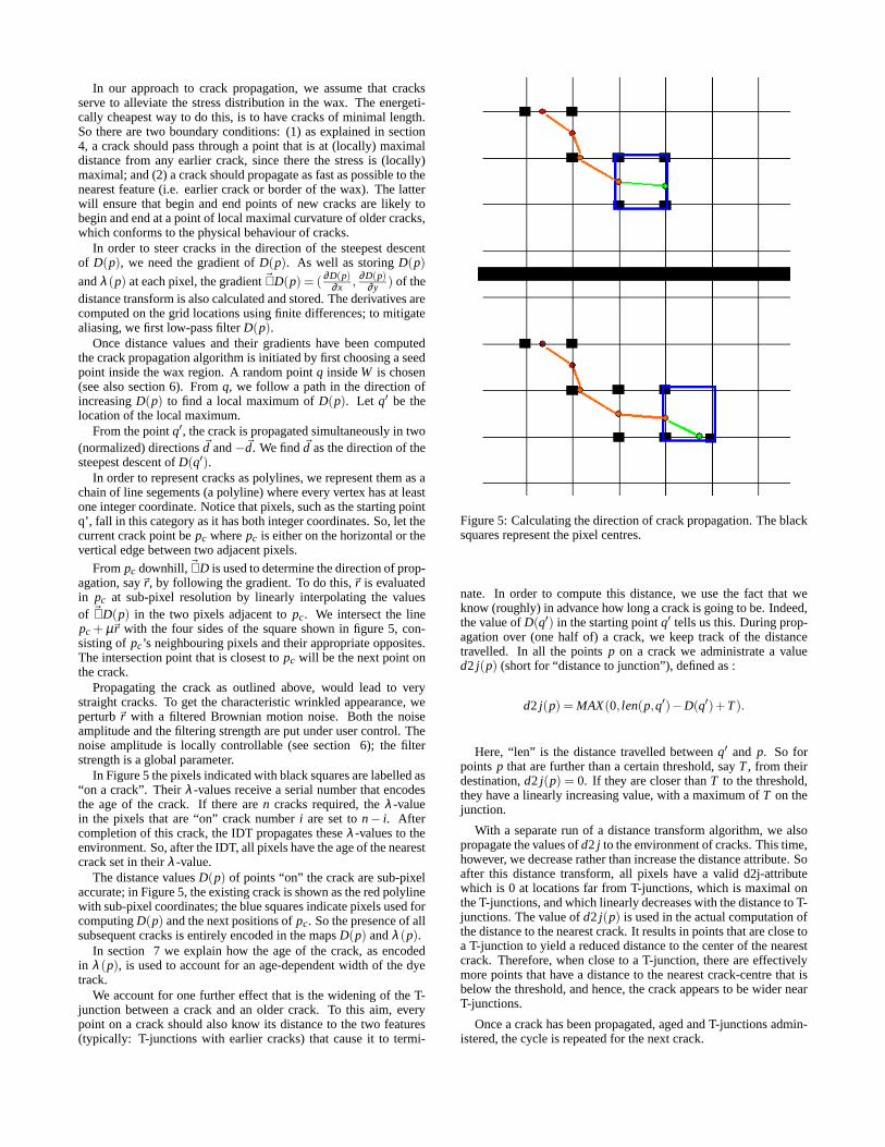
In order to represent cracks as polylines, we represent them as achain of line segements (a polyline) where every vertex has at leastone integer coordinate. Notice that pixels, such as the starting pointq’, fall in this category as it has both integer coordinates. So, let thecurrent crack point be pc where pc is either on the horizontal or thevertical edge between two adjacent pixels.

From pc downhill, ~∇D is used to determine the direction of prop-agation, say~r, by following the gradient. To do this,~r is evaluatedin pc at sub-pixel resolution by linearly interpolating the valuesof ~∇D(p) in the two pixels adjacent to pc. We intersect the linepc + µ~r with the four sides of the square shown in figure 5, con-sisting of pc’s neighbouring pixels and their appropriate opposites.The intersection point that is closest to pc will be the next point onthe crack.

Propagating the crack as outlined above, would lead to verystraight cracks. To get the characteristic wrinkled appearance, weperturb ~r with a filtered Brownian motion noise. Both the noiseamplitude and the filtering strength are put under user control. Thenoise amplitude is locally controllable (see section 6); the filterstrength is a global parameter.

In Figure 5 the pixels indicated with black squares are labelled as“on a crack”. Their λ -values receive a serial number that encodesthe age of the crack. If there are n cracks required, the λ -valuein the pixels that are “on” crack number i are set to n− i. Aftercompletion of this crack, the IDT propagates these λ -values to theenvironment. So, after the IDT, all pixels have the age of the nearestcrack set in their λ -value.

The distance values D(p) of points “on” the crack are sub-pixelaccurate; in Figure 5, the existing crack is shown as the red polylinewith sub-pixel coordinates; the blue squares indicate pixels used forcomputing D(p) and the next positions of pc. So the presence of allsubsequent cracks is entirely encoded in the maps D(p) and λ (p).

In section 7 we explain how the age of the crack, as encodedin λ (p), is used to account for an age-dependent width of the dyetrack.

We account for one further effect that is the widening of the T-junction between a crack and an older crack. To this aim, everypoint on a crack should also know its distance to the two features(typically: T-junctions with earlier cracks) that cause it to termi-

Figure 5: Calculating the direction of crack propagation. The blacksquares represent the pixel centres.

nate. In order to compute this distance, we use the fact that weknow (roughly) in advance how long a crack is going to be. Indeed,the value of D(q′) in the starting point q′ tells us this. During prop-agation over (one half of) a crack, we keep track of the distancetravelled. In all the points p on a crack we administrate a valued2 j(p) (short for “distance to junction”), defined as :

d2 j(p) = MAX(0, len(p,q′)−D(q′)+T ).

Here, “len” is the distance travelled between q′ and p. So forpoints p that are further than a certain threshold, say T , from theirdestination, d2 j(p) = 0. If they are closer than T to the threshold,they have a linearly increasing value, with a maximum of T on thejunction.

With a separate run of a distance transform algorithm, we alsopropagate the values of d2 j to the environment of cracks. This time,however, we decrease rather than increase the distance attribute. Soafter this distance transform, all pixels have a valid d2j-attributewhich is 0 at locations far from T-junctions, which is maximal onthe T-junctions, and which linearly decreases with the distance to T-junctions. The value of d2 j(p) is used in the actual computation ofthe distance to the nearest crack. It results in points that are close toa T-junction to yield a reduced distance to the center of the nearestcrack. Therefore, when close to a T-junction, there are effectivelymore points that have a distance to the nearest crack-centre that isbelow the threshold, and hence, the crack appears to be wider nearT-junctions.

Once a crack has been propagated, aged and T-junctions admin-istered, the cycle is repeated for the next crack.

Figure 6: Crack before (top) and after (bottom) aging and wideningdue to T-junctions.

6 Controlling The Process

To control the batik simulation the user supplies a series of imagesrepresenting the wax masks and the simulation computes the cracksand composites the images into an output image. There are severalcontrols that can be applied to the cracking process. Local con-trol is achieved by defining the distribution of the values of crackwidth (d(p)), crack density (ρ(p)), and crack randomness (wiggly-ness w(p)) as functions of the location p. In order to provide thesevalues the user can set the red (d(p)), green (ρ(p)), and blue (w(p))distributions in the input image. The actual colours are unimportantand greyscale images could equally well be used.

Figure 7 shows the effects of varying each of these parameters.The top map of Canada has a smooth red ramp varying from 100%red in the East to 0% in the West. The variation of d(p) in the waximage can be seen in the top image of Figure 7: the cracks are widerin the East. The apparent width of a crack is not stored explicitlybut is calculated as part of the dye application process (see 7).

The density parameter (ρ(p)) is used to control the probabilitythat a crack is created. For example, in regions of low ρ(p) fewerpoints are accepted and therefore fewer cracks generated. The al-gorithm to find the crack starting point q first selects a randompoint that lies within W . The density value, ρ(q) ranging from 0to 1, is compared against a uniform random number r ∈ [0 : 1]. Ifρ(q)3 > r the point is accepted. The cube was found empiricallyto give better results than a linear or square relationship.

The parameter w(p) is used to control the local direction taken bythe crack. In Figure 7, the cracks appear straighter in the West andfollow a more random (wiggly) path in the East as w(p) increases

from West to East.There is also a global randomness control, which can be used to

vary the direction of all the cracks. Details of how the path direc-tion is calculated are given in section 5. Other global controls areprovided by varying parameters such as overall crack width (i.e. ascaling factor affecting all cracks) and smoothness using an inter-active user interface.

In real batik the wax is often left on the cloth until the final wash-ing stage when all the wax masks are removed from the cloth. Insome cases it may be desirable to remove a wax image from thecloth in between paint/dye cycles. In this case the area of clothno longer influenced by the wax would receive more than one dyeapplication. We also simulate this process.

7 Dye Simulation

Applying the algorithm from section 5, using the control mecha-nisms as described in section 6, produces a map D(p) that repre-sents, in every point p, the distance to the nearest crack (or the bor-der of W ). It also produces a map λ (p) that represents the age (i.e.,the sequence number) of the crack nearest to p. In the present sec-tion we describe how a colour is assigned to p that corresponds tothe application of dye of a given colour to the cloth with the presentwax distribution.

There are two aspects to colour assignment: first, the computa-tion of the colour that results from mixing the dye colour with theexisting colour (which may be the original cloth colour or the colourthat resulted from applying earlier dyes) at non-protected spots, andthe computation of the intensity of the dye at a given location takingthe wax distribution into account.

7.1 A Multiplicative Colour Model for Dye Applica-

tion

We adopt a multiplicative colour model for dye colouring (see Fig-ure 8), since it more closely models the interaction between dyes,as they are applied one over the other.

This means that we associate a set of spectral reflection coeffi-cients to the cloth, say ri(p) for frequencies νi and location p, anda set of spectral transmission coefficients, say ti; j(p) to layer of dyenumber j. The resulting spectral distribution that results when illu-minating the batik with a light source with spectral distribution si isgiven by

siri(p)Π jti; j2(p),

for all i. The square accounts for the fact that the light passes twicethrough each layer of dye. In our implementation, we sample thevisible light spectrum with 3 samples: i = 1,2,3. In order to rep-resent the simulated batik in standard RGB format, we choose purespectral red, green and blue for our colour primaries ν1, ν2 and ν3.In order to visualize the resulting batik, the pure spectral compo-nents are approximated by the red, green and blue of the currentcolour reproduction device.

The spectral transmission coefficients ti; j have a negative ex-ponential dependency on the thickness of the dye layer (i.e., theamount of dye per unit area). The assumption used here is that athicker layer of dye is equivalent to two layers each of half the thick-ness. Then the reduction of the spectral intensities is the product ofthe reduction of the two individual layers, hence the exponential be-havior: f (thickness1+thickness2) = f (thickness1)∗ f (thickness2)so f must be an exponential function of the thickness.

We approximate this exponential dependency by a linear depen-dency on the dye concentration. Therefore we introduce an effec-tive dye concentration distribution, say c j(p) for dye number j atlocation p. In the next section we explain how c j(p) is computed

from D(p) and λ (p). For now we mention that c j(p) is everywherea number between 0 (no dye) and 1 (maximal dye concentration).With c j(p), we compute

ti; j(p) = 1− c j(p)(1− ti; j0),

where ti; j0 is the spectral transmission coefficient for dye number jat frequency νi when it would be applied with maximal concentra-tion.

7.2 Geometrical Aspects of the Dye Distribution

In order to compute c j(p), we adopt the assumption that dye issomewhat absorbed in cloth. This absorption gives rise to a roughlyexponential distribution [Kreyszig 1999]) near the locations whereD(p) = 0.

We approximate the negative exponential decay by a truncatedlinear function (i.e., for distances between 0 and some threshold dfrom the side of the crack the concentration linearly decays from1 to 0; for distances further than d, the concentration stays 0). Asexplained in section 6, d is allowed to vary as a function of the lo-cation p. We want to account for effects such as crack wideningdue to crack age or due to closeness to T-junctions, and we imple-ment this in the dye-depositing process by allowing d to vary as afunction of the location p, hence we use d(p).

We can compute c j(p) from D(p) by setting:

c j(p) = MAX(0,1−D(p)

d(p)).

With this formula, all cracks would give rise to dye tracks of equalwidth if d(p) is constant. In order to take crack aging into account,we set

c j(p) = MAX(0,1−D(p)λ (p)

d(p)λ0),

where λ0 is the scale parameter which globally controls crack width(see section 6). The age of the nearest crack is encoded in λ (p) suchthat older cracks correspond to larger values.

Finally we need to account for T-junction widening. In section 5it was shown how the value of d2 j(p) is computed to represent thedistance to the nearest T-junction. T-junction widening is calculatedin a similar way to crack aging, by introducing a further multiplica-tion factor, d2 j(p).

8 Results and Conclusions

The example shown in Figure 9 was made by first drawing a seriesof six wax masks, which together form the outline of the moosehead. Figure 9a shows the first wax mask (inset) and the resultantimage generated by running the crack simulation. A variation onPerlin noise [Wyvill and Novins 1999] has been used to simulatenon-homogenous dye absorption. A new wax mask has been addedin Figure 9b and the mask used in Figure 9c is an inverse mask pro-viding cracks in the background. The final moose head is the resultof combining all 6 masks in six passes through the crack simulation.

The example shown in Figure 9 was made by first drawing a se-ries of six wax masks, which together form the outline of the moosehead. Figure 9a shows the first wax mask ( read and black inset) andthe resultant image generated by running the crack simulation. Avariation on Perlin noise [Wyvill and Novins 1999] has been usedto simulate non-homogenous dye absorption. In each step as in-dicated by image groupings Figure 9a to f, a new wax mask hasbeen added. These masks are shown in red and black with the redrepsenting the waxed areas. The dyes (coloured as shown in therectangular colour swatches) are applied additively. Notice how the

additive effect of repeated dying changes the colour. In the maskused in Figure 9c is an inverse mask providing cracks in the back-ground. The final moose head is the result of combining all 6 masksin six passes through the crack simulation.

In the final image of Figure 9 some of the wax masks have beenleft in place until the end of the process, although the option existsto remove the wax at each stage. For example the wax mask ofFigure 9a, was not removed until the end of the whole process andthe area under it has a complex crack pattern, the result of multiplepasses through the crack simulation.

One of the key elements in producing a convincing visual simu-lation of the batik cracks is the process of aging and manufacturingwider cracks close to T-junctions as can be seen in Figure 9. Fora comparison of cracks generated with and without using these ef-fects see Figure 6.

From our experiments with our crack generation techniques weconclude the following:

1. The crack algorithm gives convincing batik-like cracks in flat-coloured, segmented images.

2. The various mechanisms in the batik process can be imple-mented in terms of few elementary geometric operations andimage processing operations on a purely local basis.

3. All required algorithms can be straightforwardly derived fromthe distance transform.

8.1 Limitations

In the real batik example, Figure 3b, the cracks tend to form in thenarrowest parts of the wax areas, and tend to divide the wax intolarge, roundish chunks. In the synthetic example, the cracks tendto drive right through the middle of these round areas and span thenarrow channels less frequently. The reason for this is that if a waxpiece with a narrow part is formed, the chances are large that thefirst crack as produced in our algorithm will not be in this narrowpart but rather through the middle of one of the big lobes. Thisis a consequence of our hill climbing approach, and it is a weakpoint of our algorithm. On the other hand, after subdividing piecescan soon get rounder ( i.e. more convex), and the problem is lesslikely to occur. It can be seen that the overall effect is very similarto the cracks in batik. The dye simulation is a simple approxima-tion to the actual dye process, It does not capture for example, thevariations in different types of cloth. A better dye simulation is anarea for future work. Perhaps with a more intuitive user interface,the algorithm may be useful for artists, and thus we trade the num-ber of physical phenomena we take into account for speed in oursimulation. Our results are pleasing and close to the cracks in realBatik for small computational programming effort. Judging fromother physically based cracking methods a better physical simula-tion may perhaps come closer to the appearance of the real cracksbut would be considerably more difficult to program and run muchslower.

8.2 Future Work

We have implemented these techniques as plug-in software for Pho-toshop, adding another filter to provide a new tool for artists. Theuser interface described here was merely to test the crack forma-tion process and produce the examples. Our future work includesdeveloping our own paint system that simulates the feel of the waxpainting process, including the effects of the different types of wax,and the fact that the wax tends to form blended patches as well aspractical problems such as the change in viscosity with cooling.

References

CURTIS, C. J., ANDERSON, S. E., SEIMS, J. E., FLEISHER,K. W., AND SALESIN, D. H. 1997. Computer-generated water-color. In SIGGRAPH ’97, ACM.

FEDERL, P., AND PRUSINKIEWICZ, P. 2002. Modelling fractureformation in bi-layered materials, with applications to tree barkand drying mud. Proceedings of the Thirteenth Western Com-puter Graphics Symposium.

FRASER-LU, S. 1991. Indonesian Batik: Processes, Patterns andPlaces. Oxford University Press.

GAVRILOVA, M., AND ALSUWAIYEL, M. 2001. Two algorithmsfor computing the euclidean distance transform. InternationalJournal of Image & Graphics, Special Issue on Image Process-ing 1, 4, 635–646.

GOBRON, S., AND CHIBA, N. 2001. Crack pattern simulationbased on 3d surface cellular automata. The Visual Computer 17,5, 287–309.

HERTZMANN, A., JACOBS, C. E., OLIVER, N., CURLESS, B.,AND SALESIN, D. H. 2001. Image analogies. In Proceedings ofACM SIGGRAPH 2001, Computer Graphics Proceedings, An-nual Conference Series, ACM, 327–340.

HIROTA, K., TANOUE, Y., AND KANEKO, T. 1998. Generation ofcrack patterns with a physical model. The Visual Computer 14,3, 126–137.

HIROTA, K., TANOUE, Y., AND KANEKO, T. 2000. Simulation ofthree-dimensional cracks. The Visual Computer 16, 7, 371–378.

JAIN, A. 1989. Fundamentals of Digital Image Processing, Chap-ter 2. Prentice-Hall.

KALNINS, R. D., MARKOSIAN, L., MEIER, B. J., KOWALSKI,M. A., LEE, J. C., DAVIDSON, P. L., WEBB, M., HUGHES,J. F., AND FINKELSTEIN, A. 2002. Wysiwyg npr: Drawingstrokes directly on 3d models. ACM Transactions on Graphics21, 3 (July), 755–762.

KIM, J., AND PELLACINI, F. 2002. Jigsaw image mosaics. ACMTransactions on Graphics 21, 3 (July), 657–664.

KOWALSKI, M. A., MARKOSIAN, L., NORTHRUP, J. D., BOUR-DEV, L., BARZEL, R., HOLDEN, L. S., AND HUGHES, J. F.1999. Art-based rendering of fur, grass, and trees. In Proceed-ings of SIGGRAPH 99, Computer Graphics Proceedings, AnnualConference Series, ACM, 433–438.

KREYSZIG, E. 1999. Advanced Engineering Mathematics. JohnWiley & sons, NY, ISBN 0-471-33328-x.

METAXAS, D., AND TERZOPOULOS, D. 1992. Dynamic deforma-tion of solid primitives with constraints. In Computer Graphics(Proceedings of SIGGRAPH 92), vol. 26, ACM, 309–312.

MIZUNO, S., KASAURA, T., OKOUCHI, T., YAMAMOTO, S.,OKADA, M., AND TORIWAKI, J. 2000. Automatic genera-tion of virtual woodblocks and multicolor woodblock printing.Computer Graphics Forum 19, 3 (August).

NORTON, A., TURK, G., BACON, B., GERTH, J., ANDSWEENEY, P. 1991. Animation of fracture by physical mod-eling. The Visual Computer 7, 4, 210–219.

O’BRIEN, J. F., AND HODGINS, J. K. 1999. Graphical modelingand animation of brittle fracture. In Proceedings of SIGGRAPH99, Computer Graphics Proceedings, Annual Conference Series,ACM, 137–146.

RAGHAVACHARY, S. 2002. Fracture generation on polygonalmeshes using voronoi polygons. ACM Siggraph 2002 presen-tation, 187.

SOUSA, M., AND BUCHANAN, J. W. 1999. Computer-generatedgraphite pencil rendering of 3d polygonal models. In ComputerGraphics Forum - Proceedings of Eurographics ’99, Eurograph-ics.

SOUSA, M. C., AND BUCHANAN, J. W. 1999. Computer-generated graphite pencil rendering of 3d polygonal models.Computer Graphics Forum 18, 3 (Sept.), 195–208.

TERZOPOULOS, D., AND FLEISCHER, K. 1988. Deformable mod-els. The Visual Computer 7, 4, 306 – 331.

TERZOPOULOS, D., AND FLEISCHER, K. 1988. Modeling inelas-tic deformation: Viscoelasticity, plasticity, fracture. In ComputerGraphics (Proceedings of SIGGRAPH 88), vol. 22, ACM, 269–278.

WINKENBACH, G., AND SALESIN, D. H. 1994. Computer gener-ated pen and ink illustration. In SIGGRAPH ’94, ACM.

WYVILL, G., AND NOVINS, K. 1999. Filtered noise and thefourth dimension. In SIGGRAPH 1999 Conference Abstractsand Applications, Association of Computing Machinery, Com-puter Graphics Proceedings, Annual Conference Series, ACM,242–242.

Figure 7: Each map of Canada is represented by a colour rampgoing from West to East (0-255). Crack width (red), density (green)and randomness (blue) vary as the value of the input channel variesacross each image.

Reflective Substrate: r* = 0.9 ; g* = 0.9; b* = 0.9

Transmit: r*= 1.0 ; g* = 1.0; b* = 0.25;

Transmit: r *= 0.9 ; g* = 0.9; b* = 0.4;

r= 1.0g=1.0b=1.0

r= 0.729g=0.729b=0.009

r= 0.81g=0.81b=0.0225

r= 0.81g=0.81b=0.09

r= 0.9g=0.9b=0.4

r= 0.9g=0.9b=0.1

Figure 8: How Multiplicative Colour Works, dyes may be modelledas colour filters.

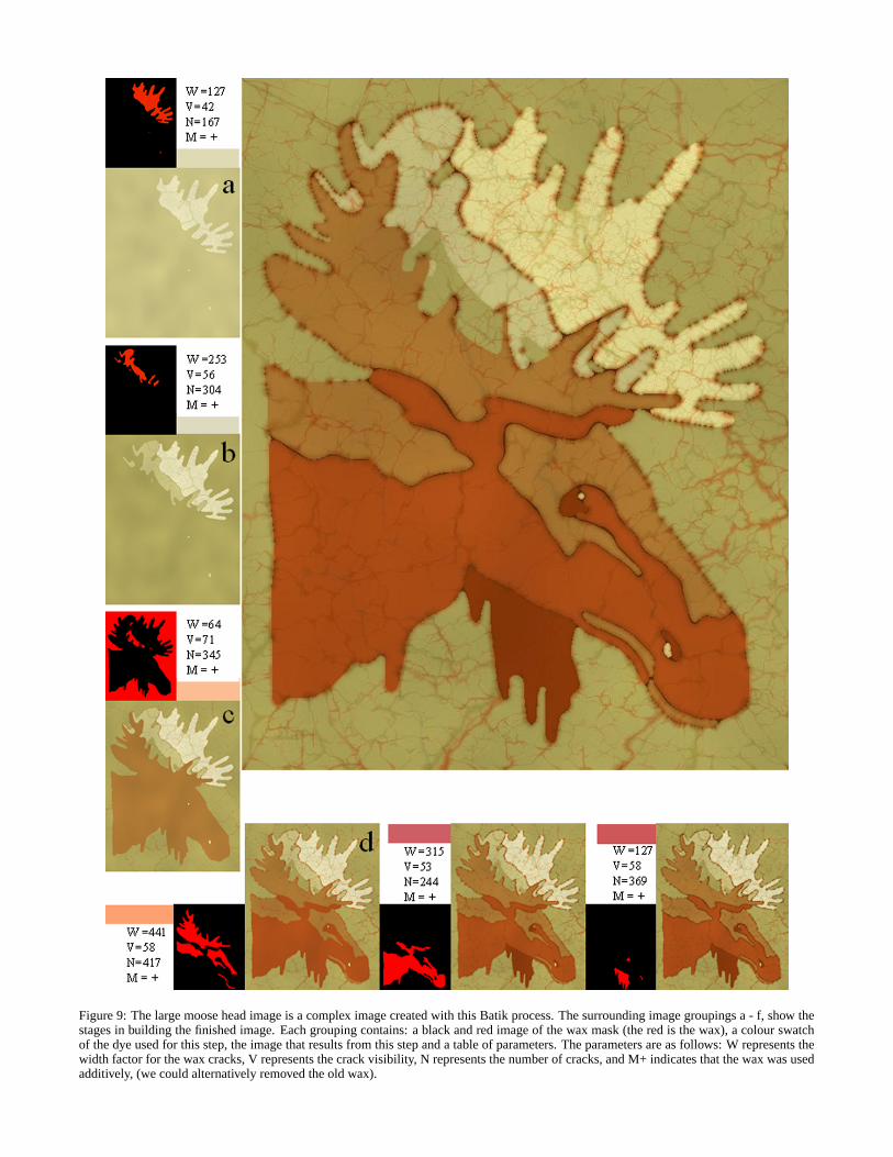
Figure 9: The large moose head image is a complex image created with this Batik process. The surrounding image groupings a - f, show thestages in building the finished image. Each grouping contains: a black and red image of the wax mask (the red is the wax), a colour swatchof the dye used for this step, the image that results from this step and a table of parameters. The parameters are as follows: W represents thewidth factor for the wax cracks, V represents the crack visibility, N represents the number of cracks, and M+ indicates that the wax was usedadditively, (we could alternatively removed the old wax).