Remotely detected vehicle mass fromengine torque-induced frame twisting

Troy R. McKayCarl SalvaggioJason W. FaulringGlenn D. Sweeney

Troy R. McKay, Carl Salvaggio, Jason W. Faulring, Glenn D. Sweeney, “Remotely detected vehicle massfrom engine torque-induced frame twisting,” Opt. Eng. 56(6), 063101 (2017),doi: 10.1117/1.OE.56.6.063101.

Remotely detected vehicle mass from enginetorque-induced frame twisting

Troy R. McKay,* Carl Salvaggio, Jason W. Faulring, and Glenn D. SweeneyRochester Institute of Technology, Chester F. Carlson Center for Imaging Science, College of Science, Digital Imaging and Remote SensingLaboratory, Rochester, New York, United States

Abstract. Determining the mass of a vehicle from ground-based passive sensor data is important for many trafficsafety requirements. This work presents a method for calculating the mass of a vehicle using ground-basedvideo and acoustic measurements. By assuming that no energy is lost in the conversion, the mass of a vehiclecan be calculated from the rotational energy generated by the vehicle’s engine and the linear acceleration of thevehicle over a period of time. The amount of rotational energy being output by the vehicle’s engine can be calcu-lated from its torque and angular velocity. This model relates remotely observed, engine torque-induced frametwist to engine torque output using the vehicle’s suspension parameters and engine geometry. The angularvelocity of the engine is extracted from the acoustic emission of the engine, and the linear acceleration ofthe vehicle is calculated by remotely observing the position of the vehicle over time. This method combinesthese three dynamic signals; engine induced-frame twist, engine angular velocity, and the vehicle’s linear accel-eration, and three vehicle specific scalar parameters, into an expression that describes the mass of the vehicle.This method was tested on a semitrailer truck, and the results demonstrate a correlation of 97.7% betweencalculated and true vehicle mass. © 2017 Society of Photo-Optical Instrumentation Engineers (SPIE) [DOI: 10.1117/1.OE.56.6.063101]

Keywords: video tracking; vehicle mass; engine torque; frame twist.

Paper 161619 received Oct. 17, 2016; accepted for publication May 23, 2017; published online Jun. 8, 2017.

1 IntroductionOverloaded commercial vehicles increase the risk of acci-dents and cause deterioration of roads and bridges. It is esti-mated that 6% of the total truck population is illegallyoverloaded.1 When trucks are loaded in excess of their maxi-mum permitted limit, they become less stable due to anelevated center of gravity which can over-strain the on-boardstability systems, increasing the potential for rollover acci-dents and jack-knifing.2 The braking capacity of a truckcan be significantly reduced due to overloading.2 Otherrisks associated with the operation of heavily laden vehiclesinclude an increased chance of a tire blowout and a higherlikelihood of fire.2 Overloaded vehicles also cause acceler-ated wear to roads and bridges. While passenger vehiclesmake up the majority of traffic on highways, trucks and otherheavy vehicles cause significantly more pavement deteriora-tion, and overloaded trucks and heavy vehicles cause a dis-proportionate amount of damage.3 For example, based on theresearch by Berthelot,4 a vehicle overloaded by 20% wouldcause more than double the damage to roadways than thesame vehicle loaded at the legal weight limit. Bridges canexperience accelerated fatigue damage due to continuedexposure to loads exceeding their design limit.2

Traditionally, overloading enforcement is carried out bythe random weighing of trucks at static weigh stations.5 Thetrucks are driven onto scales, and drivers of overloaded trucksare subjected to substantial fines. This method requires thepresence of a manned staff of weigh station employees and ittakes significant time to weigh the truck and issue the citationto the driver.2 As a result, not all trucks are weighed, which

leads to more drivers pushing the limits and driving over-loaded. A method of measuring the mass of a vehicle usinga ground-based, real-time, imaging, and acoustic sensor sys-tem would increase efficiency and allow overloaded vehiclesto be identified and singled out. This would reduce the costsassociated with manning a weigh station, allow appropriatelyloaded vehicles to avoid unwarranted delays, prevent accel-erated damage to roadways and bridges, and protect the pub-lic from the dangers presented by these overloaded vehicles.This paper discusses the work performed to develop amethod for calculating the mass of a vehicle, remotely,using ground-based imaging and acoustic sensors.

2 BackgroundThe method described here exploits Newton’s third law tocalculate the total mass of a vehicle from measurements ofits linear velocity and the rotational energy output by itsengine. Consider a typical rear-wheel drive vehicle at restwith its engine idling. To move forward, the rotationalenergy generated by the engine is transferred to the transmis-sion via the release of the clutch, where the transmissionincreases the rotational torque and reduces the rotationalvelocity. The output of the transmission turns the drive shaft,which in turn rotates the rear axle’s pinion gear, which turnsthe rear wheels and propels the vehicle. The total transferefficiency of this conversion from rotational power to linearpower at low linear velocities is determined predominatelyby the transfer efficiency of the transmission.6 A typicaltransmission has an efficiency in the range of 0.85 to 0.95and varies based on gear.6

Per Newton’s third law, which states that for every actionthere is an equal and opposite reaction, the action of the

*Address all correspondence to: Troy McKay, E-mail: troy@hyperspectralsolutions.com 0091-3286/2017/$25.00 © 2017 SPIE

Optical Engineering 063101-1 June 2017 • Vol. 56(6)

Optical Engineering 56(6), 063101 (June 2017)

applied torque results in an equal and opposite reactiontorque. This reaction torque is opposed by the vehicle’s sus-pension as the vehicle’s frame rotates relative to its axles. Foran engine mounted parallel to the drive shaft, known as alongitudinal engine, this frame twist would manifest as acounter-clockwise rotation (viewing the vehicle head on).The magnitude of this rotation is small, typically less than2 deg during heavy acceleration. An example of this enginetorque-induced frame twisting can be seen in Fig. 1.

Measurements of the engine torque-induced frame twistcombined with acoustic measurements of the engine’sspeed can be used to calculate the energy generated by theengine over a period of time. Given a dry, flat, roadway, andassuming all of the rotation energy generated by the engine isconverted into the vehicle’s linear kinetic energy, the mass ofthe vehicle can be determined through measurements of thevehicle’s change in velocity. Equation (1) shows the relation-ship between kinetic energy and mass for linear motion;where KE is the linear kinetic energy of the vehicle, m isthe total mass of the vehicle, and x 0 is the linear velocityof the vehicle. By measuring the rotational power outputby the vehicle’s engine over a period of time and measuringthe change in linear velocity of the vehicle over the sameperiod of time, the mass of the vehicle can be calculated

EQ-TARGET;temp:intralink-;e001;63;306KE ¼ 1

2m · ðx 0Þ2: (1)

When the engine is applying torque to the vehicle frameτE, the frame twists relative to the axles and the vehicle’ssuspension springs are compressed and stretched as shownin Fig. 2. This compression and stretching of the suspensionsprings cause pushing and pulling forces to be applied at thepoints where the frame and suspension are joined. Theamount of torque generated by these forces τF is dependenton their distance from the axis of rotation r and the amount offrame twist θ as described by Eq. (2) (the cosine termaccounts for the force applied nonperpendicularly to theradial axis).7 The forces F1 and F2 are generated by thevehicle’s suspension and can be described in terms of theframe twist and the total suspension spring constant ks asgiven in Eqs. (3) and (4). By combining these equations, thetorque generated by the suspension can be described as afunction of frame twist [Eq. (5)]. Since the torque the engineis applying to the frame is equal in magnitude and opposite indirection to the torque the suspension is applying on the

frame, the engine torque can be described as a function ofthe frame twist using the relationship described in Eq. (6)

EQ-TARGET;temp:intralink-;e002;326;508τFðtÞ ¼ r · cos½θðtÞ þ θ0� · ðF2 − F1Þ; (2)

EQ-TARGET;temp:intralink-;e003;326;478F1ðtÞ ¼ −ks · r · tan½θðtÞ�

2; (3)

EQ-TARGET;temp:intralink-;e004;326;442F2ðtÞ ¼ks · r · tan½θðtÞ�

2; (4)

EQ-TARGET;temp:intralink-;e005;326;406τFðtÞ ¼ ks · r2 · cos½θðtÞ þ θ0� · tan θðtÞ; (5)

EQ-TARGET;temp:intralink-;e006;326;380τEðtÞ ¼ −ks · r2 · cos½θðtÞ þ θ0� · tan θðtÞ: (6)

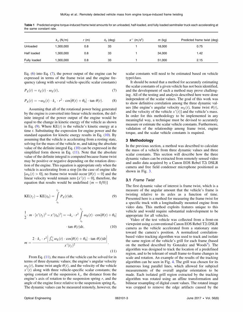
The expected amount of engine torque-induced frametwist was calculated for an unloaded, half-loaded, and fullyloaded semitrailer truck accelerating at a constant rate andcan be seen in Table 1. For this calculation, the total suspen-sion spring constant ks was estimated for a typical semitrailertruck having four leaf springs (two in the front and two in therear). The engine and suspension geometry parameters (r andθ0) were estimated for a typical semitrailer truck. This esti-mation is predicated on the assumption of a flat road andgood driving conditions. This frame-twist angle estimationdoes not take into consideration the efficiency of the trans-mission, and as a result, will be slightly overestimated. Theseestimated results show the expected engine torque-inducedframe twist values to range from 0.75 deg, for an unloadedsemitrailer truck, to 2.15 deg for a fully loaded semitrailertruck. These estimates predict that the frame twist signatureshould be large enough to measure remotely.

Now that the torque being created by the engine has beendescribed in terms of the amount of rotational deflection ofthe vehicle frame, the next step is to describe how much rota-tional power the engine is creating. Rotational power isdefined by the torque and angular velocity of the rotatingshaft [Eq. (7)].8 To calculate the power output of the engine,the angular velocity of the engine ωEðtÞ must be measured.The angular velocity of the engine can be determined directlyfrom the acoustic emissions of the engine. By substituting

Fig. 1 (a) The vehicle at rest with no engine-induced torque and(b) the vehicle with engine torque-induced frame twist as the vehiclebegins to accelerate from a resting state.

Fig. 2 Longitudinal engine imparting torque τE to the vehicle framecausing it to twist until the torque generated by the suspension forces(F 1 and F 2) are sufficient to match.

Optical Engineering 063101-2 June 2017 • Vol. 56(6)

McKay et al.: Remotely detected vehicle mass from engine torque-induced frame twisting

Eq. (6) into Eq. (7), the power output of the engine can beexpressed in terms of the frame twist and the engine fre-quency (along with several vehicle-specific scalar constants)

EQ-TARGET;temp:intralink-;e007;63;594PEðtÞ ¼ τEðtÞ · ωEðtÞ; (7)

EQ-TARGET;temp:intralink-;e008;63;564PEðtÞ ¼ −ωEðtÞ · ks · r2 · cos½θðtÞ þ θ0� · tan θðtÞ: (8)

Assuming that all of the rotational power being generatedby the engine is converted into linear vehicle motion, the def-inite integral of the power output of the engine would beequal to the change in kinetic energy of the vehicle as shownin Eq. (9). Where KEðtÞ is the vehicle’s kinetic energy at atime t. Substituting the expression for engine power and thestandard equation for kinetic energy results in Eq. (10). Byassuming that the vehicle is accelerating from a resting state,solving for the mass of the vehiclem, and taking the absolutevalue of the definite integral Eq. (10) can be expressed in thesimplified form shown in Eq. (11). Note that the absolutevalue of the definite integral is computed because frame twistmay be positive or negative depending on the rotation direc-tion of the engine. This equation is appropriate only when thevehicle is accelerating from a stop [in the case of engine idle[ωEðtÞ > 0], no frame twist would occur [θðtÞ ¼ 0] and thelinear velocity would remain zero [x 0ðtÞ ¼ 0], therefore, theequation that results would be undefined ðm ¼ 0∕0Þ]

EQ-TARGET;temp:intralink-;e009;63;339KEðtfÞ − KEðt0Þ ¼Ztft0

PEðtÞdt; (9)

EQ-TARGET;temp:intralink-;e010;63;286

1

2· m · ½x 0ðtfÞ2 − x 0ðt0Þ2� ¼ −ks · r2

Ztft0

ωEðtÞ · cos½θðtÞ þ θ0�

· tan θðtÞdt; (10)

EQ-TARGET;temp:intralink-;e011;63;215m ¼2 · ks · r2

��� R tft0 ωEðtÞ · cos½θðtÞ þ θ0� · tan θðtÞdt

���x 0ðtfÞ2

:

(11)

From Eq. (11), the mass of the vehicle can be solved for interms of three dynamic values; the engine’s angular velocityωEðtÞ, frame twist angle θðtÞ, and the velocity of the vehiclex 0ðtÞ along with three vehicle-specific scalar constants; thespring constant of the suspension ks, the distance from theengine’s axis of rotation to the suspension spring r, and theangle of the engine force relative to the suspension spring θ0.The dynamic values can be measured remotely, however, the

scalar constants will need to be estimated based on vehicletype/class.

It should be noted that a method for accurately estimatingthe scalar constants of a given vehicle has not been identified,and the development of such a method may prove challeng-ing. All of the testing and analysis described here were doneindependent of the scalar values. The goal of this work wasto show definitive correlation among the three dynamic val-ues [the engine’s angular velocity ωEðtÞ, frame twist θðtÞ,and the velocity of the vehicle x 0ðtÞ] and the vehicle’s mass.In order for this methodology to be implemented in anymeaningful way, a technique must be devised to accuratelymeasure or estimate the scalar vehicle constants. Furthermore,validation of the relationship among frame twist, enginetorque, and the scalar vehicle constants is required.

3 MethodologyIn the previous section, a method was described to calculatethe mass of a vehicle from three dynamic values and threescalar constants. This section will describe how the threedynamic values can be extracted from remotely sensed videoand audio data acquired by a Canon EOS Rebel T2i DSLRcamera and free field condenser microphone positioned asshown in Fig. 3.

3.1 Frame Twist

The first dynamic value of interest is frame twist, which is ameasure of the angular amount that the vehicle’s frame istwisting relative to its axles as a function of time.Presented here is a method for measuring the frame twist fora specific truck with a longitudinally mounted engine fromvideo data. This method exploits features unique to thisvehicle and would require substantial redevelopment to beappropriate for all vehicles.

Video of the test vehicle was collected from a front-onviewpoint using a conventional Canon EOS Rebel T2i DSLRcamera as the vehicle accelerated from a stationary statetoward the camera’s position. A normalized correlation-based video tracking algorithm was used to track and isolatethe same region of the vehicle’s grill for each frame (basedon the method described by Gonzalez and Woods9). Thealgorithm was designed to track the location of a predefinedregion, and to be tolerant of small frame-to-frame changes inscale and rotation. An example of the results of the trackingalgorithm can be seen in Fig. 4. The grill was chosen for itsnumerous long parallel lines, which allowed for subpixelmeasurements of the overall angular orientation to bemade. Each isolated grill region extracted by the trackingalgorithm was rotated using an affine transformation andbilinear resampling of digital count values. The rotated imagewas cropped to remove the edge artifacts caused by the

Table 1 Predicted engine torque-induced frame twist amounts for an unloaded, half-loaded, and fully loaded semitrailer truck each accelerating atthe same constant rate.

ks (N∕m) r (m) θ0 (deg) x 0 0 (m∕s2) m (kg) Predicted frame twist (deg)

Unloaded 1,300,000 0.8 33 1 18,000 0.75

Half loaded 1,300,000 0.8 33 1 34,000 1.42

Fully loaded 1,300,000 0.8 33 1 51,000 2.15

Optical Engineering 063101-3 June 2017 • Vol. 56(6)

McKay et al.: Remotely detected vehicle mass from engine torque-induced frame twisting

rotation, and the summed standard deviation was calculatedfor each vertical column of pixels in the cropped region using

EQ-TARGET;temp:intralink-;e012;63;395V ¼Xmj¼1

ffiffiffiffiffiffiffiffiffiffiffiffiffiffiffiffiffiffiffiffiffiffiffiffiffiffiffiffiffiffiffiffiffi1

n

Xni¼1

ðxi;j − x̄jÞ2s

; (12)

where V is a scalar value that quantifies the total vertical vari-ability of the image, m is the number of columns of pixels inthe image, n is the number of rows of pixels in the image, xi;jis the intensity value for the pixel at location (i; j), and x̄j isthe average intensity value of the pixels in column j. Thisscalar value V would have a value of zero if each row of theimage was identical. This was repeated for a range of rotation

values bounding the expected rotation of the vehicle duringits acceleration period. The rotation that resulted in the mini-mum scalar sum was selected as the rotation of the grill (rel-ative to the vertical image axis). The process was repeated foreach image frame as the vehicle was in motion. Figure 5shows this approach for determining the vehicle’s rotation.

3.2 Position

The second dynamic value of interest is the position of thevehicle as a function of time. Presented here is a method formeasuring the position of a specific vehicle from video data.This method exploits features unique to a specific vehicleand a priori knowledge of these features. There are othertechniques that could be used to accurately measure a vehicle’sposition as a function of time that would be more universallyapplicable, but would require additional equipment (e.g.,LiDAR, ultrasonic distance sensor).

Using the same video sequence exploited in the previoussection, the camera-to-vehicle distance as a function of timewas calculated by observing the spacing of the grill, in pix-els, utilizing Fourier analysis. After the grill images wererotated so the grill runs perpendicular to the horizontal imageaxis, the average of each vertical column was taken, resultingin an averaged grill profile. A Hamming window was appliedto the profile to reduce instances of aliasing. The magnitudeof the Fourier transform was then taken and the peak fre-quency was identified as the frequency of the grill, theinverse of this frequency representing the period (in pixels).See Fig. 6 for an example of this process.

Fig. 3 Diagram of the camera, microphone, and vehicle position during the experiment.

Fig. 4 An image frame with the extracted grill region identified.

Fig. 5 In order to determine the angle of rotation of the grill, (a) the unrotated grill image is rotated througha range of image rotations from −5 deg to 5 deg, (b) recording the vertical variability as a function ofrotation angle. (c) The minimum depicted in the plot corresponds to the position where the grill standsperpendicular to the horizontal image axis.

Optical Engineering 063101-4 June 2017 • Vol. 56(6)

McKay et al.: Remotely detected vehicle mass from engine torque-induced frame twisting

The grill spacing in pixels was calculated for each videoframe using this approach. The camera-to-vehicle distancefor each frame was then calculated using Eq. (13), where dis the camera-to-vehicle distance, S is the grill spacing inmeters, f is the focal length of the camera in meters, ρ is thepixel pitch of the camera’s detector array in meters, and N isthe grill spacing in pixels (the period). While the processdescribed here required a priori knowledge of the grill spac-ing, this method could be adapted to work on any featurecontaining a repetitive, regularly spaced, pattern as longas the camera-to-vehicle distance is known at one point dur-ing the collection, or the dimensions of another feature on thevehicle is known (e.g., license plate)

EQ-TARGET;temp:intralink-;e013;63;442d ¼ S · fρ · N

: (13)

3.3 Engine Speed

The final dynamic value of interest is engine speed as a func-tion of time. Presented here is a method for measuring theengine speed of a specific vehicle from acoustic data. Thismethod requires a priori knowledge of the vehicle’s enginesize, specifically the number of cylinders. To make thismethod effective for use on all vehicles, it would need to bemodified to determine the number of cylinders from theacoustic data. Preliminary work has been done that suggeststhat it is possible to calculate the number of cylinders anengine has based on its acoustic signal through analysis ofthe harmonics.10

Acoustic measurements of the test vehicle were collectedusing a microphone mounted near the path of the vehicle.The audio data were used to calculate the engine speed, again

utilizing Fourier analysis. The audio data were first extractedfrom the video file and converted into a time-based pressuresignal. A 0.3-s window of data was selected starting at timezero, a Hamming window was applied, and the magnitude ofthe Fourier transform was taken resulting in a power spectra.The operating frequency of the engine was calculated bylocating the peaks in the power spectra associated with itsthird, sixth, and ninth harmonic and then dividing the fre-quency by the harmonic number. For example, if the thirdharmonic was found at 30 Hz, the engine frequency wouldbe 10 Hz. Three harmonics were used because no single har-monic was found to be reliably persistent in the audio signal.The initial search locations were restricted to frequenciescorresponding to the typical idling frequency of a large dieselengine, ∼420 to 960 rpm (or 7 to 16 Hz). Once the initialengine frequency was identified, the window of data wasmoved forward in time by 1 ms and the process was repeated,with the search area for each harmonic being substantiallyrestricted to within 5 Hz of the previous harmonic. If thethree harmonics agreed well, the average of the three calcu-lated engine frequency values was used. If one of the threeharmonics did not agree, it was discarded. If none of the har-monics agreed well, the lowest order (third harmonic) wasselected and used to calculate the engine frequency. Thisprocess continued until the entire pressure signal was proc-essed, resulting in an engine frequency versus time signal.An example of this process is shown in Fig. 7.

After the acoustic data were processed into an engine fre-quency versus time signal, they needed to be synchronizedwith the data signals extracted from the video (frame twistand camera-to-vehicle distance). This synchronization wasachieved through frame-by-frame analysis of on-board video

Fig. 6 To calculate the grill spacing, (a) the average grill intensity profile is demeaned and (b) a Hammingwindow is applied. (c) The power spectra is then calculated and used to find the frequency of the grill.

Fig. 7 To calculate engine velocity, (a) the raw acoustic signal is demeaned and (b) a Hamming windowis applied. (c) The power spectra is then calculated and used to find the third, sixth, and ninth harmonic.

Optical Engineering 063101-5 June 2017 • Vol. 56(6)

McKay et al.: Remotely detected vehicle mass from engine torque-induced frame twisting

taken from inside the truck during each test run that capturedthe engine rpm and the vehicle speed from the vehicle’sinstrument panel. A still frame from this video can be seenin Fig. 8. This method of synchronization was both challeng-ing and imprecise, and it is highly recommended that anyfuture testing utilizes a synchronized data acquisition systemto mitigate the need for this approach.

4 ResultsTwo full-scale field tests were carried out to test the validityof the mass estimation method and the practicality of theremote sensing techniques. Each test was carried out at theSavannah River Site, a United States Department of Energyfacility located in Aiken, South Carolina. Both field tests

used the same semitrailer truck in three load conditions;the recommended maximum load (40 tons), half the recom-mended maximum load (20 tons), and no load (emptytrailer). Each load mass was determined by loading the trailerwith large concrete and metal blocks of known masses. Aminimum of three test runs was completed for each load con-dition during both field tests. The first field test utilized aconsumer-quality Canon EOS Rebel T2i DSLR camera posi-tioned in front of the vehicle to collect video and audio as thetest vehicle accelerated from a stop. The video was collectedat 30 frames-per-second, and the audio was collected at44.1 kHz. The second field test utilized a Vision ResearchPhantom v5.1 high-speed video camera in a similar positionand collected video at a rate of 1200 frames-per-second. Thesecond test utilized a PCB Piezotronics free-field condensermicrophone to collect the audio data at a rate of 52 kHz.

For each test run, the video and audio data were processedusing the methods described in the previous section andresulted in angular frame twist, position, and engine speedas a function of time. An example of a processed datasetfrom the first field test can be seen in Fig. 9 and an exampleset from the second field test can be seen in Fig. 10. Theprimary difference between the processed datasets fromthese two independent field tests was the collection duration.The high-speed camera was able to collect only for a shorttime (∼2 s) due to internal memory limitations and the highframe rate. This resulted in several datasets being deemedunusable because the high-speed video was triggered toolate, not capturing the initial frame twist of the vehicle. It iscritical that the vehicle is measured while the frame is ina relaxed state; the frame twist at this time correlates to

Fig. 8 An example of the on-board video of the vehicle’s instrumentpanel captured during each test run.

Fig. 9 (a) The angular frame twist, (b) vehicle position, and (c) engine speed of the unloaded test vehicleaccelerating from a stop during the first field test.

Fig. 10 (a) The angular frame twist, (b) vehicle position, and (c) engine speed of the unloaded testvehicle accelerating from a stop during the second field test.

Optical Engineering 063101-6 June 2017 • Vol. 56(6)

McKay et al.: Remotely detected vehicle mass from engine torque-induced frame twisting

the zero-torque condition, and all subsequent measurementsmust be made relative to this initial state. For many of thedata sets from the second field test, the high-speed video wasinitiated after the frame began to twist, but before the vehiclebegan moving forward (there is typically a 0.5- to 1-s offsetbetween when the frame first twists and the first measurableforward movement of the vehicle occurs). Due to this lateinitiation of the high-speed video, it was impossible to deter-mine the amount of frame twist associated with the zerotorque condition. To mitigate this, the vehicle should beobserved for a considerable time, 2 to 3 s prior to acceler-ation in order to identify the zero-torque frame twist position.It should be noted that the vehicle does not need to be com-pletely stopped in order to identify the zero-torque condition,it must simply not be accelerating at this initial observation.

The spring constant ks was not known for the test vehicle.As a result, Eq. (11) needed to be modified slightly toaccount for the unknown spring constant, yielding Eq. (14)which was used to calculate the mass-to-spring constant ratioof the test vehicle for each test run. The final time tf wasidentified as the time when the test vehicle reached its peakvelocity and the values for r and θ0 were estimated to be 0.8 mand 33 deg, respectively. The results for the first and secondfield tests can be seen in Figs. 11 and 12, respectively

EQ-TARGET;temp:intralink-;e014;326;752

mks

¼ 2 · r2�� R tf

t0 ωEðtÞ · cos½θðtÞ þ θ0� · tan θðtÞdt��x 0ðtfÞ2

: (14)

5 ConclusionsRemotely collected video and audio data were used to cal-culate a vehicle’s position, engine torque-induced frametwist, and engine speed. These signals were used to calculatethe vehicle’s mass-to-spring constant ratio. The resultsdepicted for the second field test (Fig. 12) show a significantreduction in this mass-to-spring constant ratio when com-pared to the first field test (Fig. 11). The reduction in thisratio was approximately a factor of three, which suggests thatthree times as much energy was required, during the first testas compared to the second test, to change the velocity of thetest vehicle by the same amount. This discrepancy was inves-tigated and it was determined that the data for the first fieldtest were collected while the test vehicle was driving slightlyuphill. Even a mild to moderate incline of 3 deg to 5 degwould account for the discrepancy observed between the twotests. To account for this, future testing would need to bedone on roads with an incline of zero degrees, or the inclinewould need to be incorporated into Eq. (14). The equationfor the mass-to-spring constant ratio incorporating the effectsof the road surface inclination angle is given here

EQ-TARGET;temp:intralink-;e015;326;470

mks

¼ r2�� R tf

t0 ωEðtÞ · cos½θðtÞ þ θ0� · tan θðtÞdt��h12· x 0ðtfÞ2

iþ f−g · ½hðtfÞ − hðt0Þ�g

; (15)

where g is the force due to gravity, hðtfÞ is the vehicle’selevation at time tf, and hðt0Þ is the vehicle’s elevation attime t0. This equation shows that a small change in elevationcan require a significant amount of energy. For example, anincrease in elevation of 5 cm would require the same amountof energy as a change in velocity of 1 m∕s.

The correlation between the calculated vehicle mass-to-spring constant ratio and the true vehicle mass was foundto be very good for both field tests. The correlation coeffi-cient was calculated to be 97.7% for the first test and 99.7%for the second test. This reflects a very good correlationbetween the remotely determined values and the true massdata for both experiments. This strong correlation doesnot reflect accuracy in mass estimation, only that the mea-sured data agreed very well with the actual vehicle mass towithin a scale factor. In order for this methodology to calcu-late vehicle mass, work needs to be done to develop and val-idate a means of measuring or estimating this scale factor.

The results of this testing showed strong correlation andgood within-test repeatability. However, there are multipleareas in which improvements could be made. First, it is criti-cal that all of the measured signals are synchronized. Themost accurate method of achieving this synchronization isby utilizing a single data acquisition system for all measure-ments (audio and video). Second, the data acquisition systemmust begin measuring the vehicle at least 2 s prior to anyforward motion or acceleration from a constant velocity ini-tial motion state. This will ensure that the zero-torque con-dition is captured. Third, the grade of the road where the testvehicle is being operated should be measured precisely andaccounted for using Eq. (15). Finally, observation of the testvehicle should be extended. Increasing the measurement

17690 34382 510750

0.05

0.1

0.15

0.2

0.25

0.3

0.35

m/k

s

True mass (kg)

Fig. 11 The calculated mass-to-spring constant ratio for each test runin the first field test versus the true test vehicle mass.

17690 34382 510750

0.02

0.04

0.06

0.08

0.1

True mass (kg)

m/k

s

Fig. 12 The calculated mass-to-spring constant ratio for each test runin the second field test versus the true test vehicle mass.

Optical Engineering 063101-7 June 2017 • Vol. 56(6)

McKay et al.: Remotely detected vehicle mass from engine torque-induced frame twisting

window to 10 to 15 s should improve the overall effective-ness of the system and make the measurements more robustto noise and measurement error. This could be achieved byreducing the frame rate of the video acquisition system, asthe 1200 frames-per-second rate of the Vision ResearchPhantom v5.1 camera proved to be faster than is required.A more reasonable 100 to 300 frame rate camera should pro-vide more than adequate temporal resolution.

AcknowledgmentsThe authors would like to thank the United States Depart-ment of Energy, National Nuclear Security Administration,and Office of Defense Nuclear Nonproliferation (NA-22) fortheir support of this work under Contract No. DE-AC09-08SR22470/AC799980. Special thanks are expressed toDr. Alfred Garrett, Dr. David Coleman, and Dr. LarryKoffman of the Savannah River National Laboratory for theirinvaluable assistance in facilitating the field experiments car-ried out at the Savannah River Site in Aiken, South Carolina.

References

1. M. Ghosn et al., “Effects of overweight vehicles on NYSDOT infra-structure,” Tech. Rep. (2015).

2. B. Jacob and V. Feypell-de La Beaumelle, “Improving truck safety:potential of weigh-in-motion technology,” IATSS Res. 34(1), 9–15(2010).

3. K. Dey et al., “Estimation of pavement and bridge damage costs causedby overweight trucks,” Transp. Res. Rec. J. Transp. Res. Board 2411,62–71 (2014).

4. D. Podborochynski et al., “Quantifying incremental pavement damagecaused by overweight trucks,” in Conf. on Exhibition of the Transpor-tation Association of Canada (2011).

5. K. Helmi, T. Taylor, and F. Ansari, “Shear force–based method andapplication for real-time monitoring of moving vehicle weights onbridges,” J. Intell. Mater. Syst. Struct. 26(5), 505–516 (2015).

6. A. Irimescu, L. Mihon, and G. Pãdure, “Automotive transmission effi-ciency measurement using a chassis dynamometer,” Int. J. Automot.Technol. 12(4), 555–559 (2011).

7. F. Beer, E. Johnston, and J. DeWolf,Mechanics of Materials, McGraw-Hill, New York (2002).

8. J. Walker et al., Fundamentals of Physics, Wiley, New York (2008).9. R. Gonzalez and R. Woods,Digital Image Processing, Pearson/Prentice

Hall, Upper Saddle River, New Jersey (2008).10. T. McKay, Detection of Anomalous Vehicle Loading, PhD Thesis,

Rochester Institute of Technology (2016).

Troy R. McKay received his BA degree in applied physics from SUNYGeneseo in 2003, his MS degree in electrical engineering from SUNYBuffalo in 2007, and his PhD in imaging science from the RochesterInstitute of Technology in 2016. He is currently the founder andpresident of Hyperspectral Solutions, LLC.

Carl Salvaggio received his BS and MS degrees in imaging sciencefrom the Rochester Institute of Technology (RIT) in 1987, and his PhDin environmental resource engineering in 1994 from the State Univer-sity of New York College of Environmental Science and Forestry atSyracuse University. From 1994 to 2002, he worked on model vali-dation and database development for the defense intelligence com-munity. Since 2002, he has been a professor of imaging science atRIT.

Jason W. Faulring received his BS degree in computer engineeringfrom the Rochester Institute of Technology (RIT) in 2003. As a seniorsystems engineer at the Remote Sensing Laboratory of RIT from2003 to 2015, he developed innovative airborne and ground-basedsensing systems for the lab’s research efforts. He is currently a seniorengineer and partner at AppliedLogix, LLC developing custom hard-ware and software solutions.

Glenn D. Sweeney received his BS degree in imaging science fromthe Rochester Institute of Technology in 2013, and his MSc degree incolor science from the CIMET University consortium in 2015. Aftergraduation, he has entered the workforce designing image quality testequipment for mobile camera systems.

Optical Engineering 063101-8 June 2017 • Vol. 56(6)

McKay et al.: Remotely detected vehicle mass from engine torque-induced frame twisting