Remote sensing space weather events: the AARDDVARK network · Remote sensing space weather events:...
40
Remote sensing space weather events: the AARDDVARK network Mark A. Clilverd 1 , Craig J. Rodger 2 , Neil R Thomson 2 , James B. Brundell 3 , Thomas Ulich 4 , János Lichtenberger 5 , Neil Cobbett 1 , Andrew B. Collier 6 , Frederick W. Menk 7 , Annika Seppälä 1,8 , Pekka T. Verronen 8 , and Esa Turunen 4 Abstract. The Antarctic-Arctic Radiation-belt (Dynamic) Deposition - VLF Atmospheric Research Konsortium (AARDDVARK) provides a network of continuous long-range observations of the lower-ionosphere in the polar regions. Our ultimate aim is to develop the network of sensors to detect changes in ionization levels from ~30-90 km altitude, globally, continuously, and with high time resolution, with the goal of increasing the understanding of energy coupling between the Earth's atmosphere, the Sun, and space. This science area impacts our knowledge of space weather processes, global atmospheric change, communications, and navigation. The joint New Zealand-United Kingdom AARDDVARK is a new extension of a well-established experimental technique, allowing long-range probing of ionization changes at comparatively low altitudes. Most other instruments which can probe the same altitudes are limited to essentially overhead measurements. At this stage AARDDVARK is essentially unique, as similar systems are only deployed at a regional level. The AARDDVARK network has contributed to the scientific understanding of a growing list of space weather science topics including solar proton events, the descent of NO x into the middle atmosphere, substorms, precipitation of energetic electrons by plasmaspheric hiss and EMIC waves, the impact of coronal mass ejections upon the radiation belts, and relativistic electron microbursts. Future additions to the receiver network will increase the science potential and provide global coverage of space weather event signatures.
Transcript of Remote sensing space weather events: the AARDDVARK network · Remote sensing space weather events:...
Remote sensing space weather events: the AARDDVARK network
Mark A. Clilverd1, Craig J. Rodger2, Neil R Thomson2, James B. Brundell3, Thomas
Ulich4, János Lichtenberger5, Neil Cobbett1, Andrew B. Collier6, Frederick W.
Menk7, Annika Seppälä1,8, Pekka T. Verronen8, and Esa Turunen4
Abstract. The Antarctic-Arctic Radiation-belt (Dynamic) Deposition - VLF Atmospheric
Research Konsortium (AARDDVARK) provides a network of continuous long-range
observations of the lower-ionosphere in the polar regions. Our ultimate aim is to develop the
network of sensors to detect changes in ionization levels from ~30-90 km altitude, globally,
continuously, and with high time resolution, with the goal of increasing the understanding of
energy coupling between the Earth's atmosphere, the Sun, and space. This science area impacts
our knowledge of space weather processes, global atmospheric change, communications, and
navigation. The joint New Zealand-United Kingdom AARDDVARK is a new extension of a
well-established experimental technique, allowing long-range probing of ionization changes at
comparatively low altitudes. Most other instruments which can probe the same altitudes are
limited to essentially overhead measurements. At this stage AARDDVARK is essentially unique,
as similar systems are only deployed at a regional level. The AARDDVARK network has
contributed to the scientific understanding of a growing list of space weather science topics
including solar proton events, the descent of NOx into the middle atmosphere, substorms,
precipitation of energetic electrons by plasmaspheric hiss and EMIC waves, the impact of
coronal mass ejections upon the radiation belts, and relativistic electron microbursts. Future
additions to the receiver network will increase the science potential and provide global coverage
of space weather event signatures.
1. Introduction
The Antarctic-Arctic Radiation-belt (Dynamic) Deposition - VLF Atmospheric Research
Konsortium (AARDDVARK) is a global network of radio receivers designed to make continuous
long-range observations of the lower-ionosphere at mid- to high-latitude regions. The network of
cheap, easy to install, easy to maintain sensors use pre-existing manmade very low frequency
radio waves (VLF) to detect changes in ionization levels from ~30-90 km altitude, continuously,
and with high time resolution. The network’s goal is to increase the understanding of energy
coupling between the Earth's atmosphere, the Sun, and space. The part of the electromagnetic
spectrum described as VLF generally spans 3 - 30 kHz. Most ground-based observations in the
VLF band are dominated by the strong impulsive signals radiated by lightning discharges. These
produce significant electromagnetic power from a few hertz to several hundred megahertz
[Magono, 1980], with the bulk of the energy radiated in the VLF frequency band. At VLF such
pulses are termed "atmospherics", or simply ‘sferics’. In addition to ‘sferics’, at frequencies
>10 kHz manmade transmissions from communication and navigation transmitters can be
observed in almost every part of the world.
Most of the energy radiated by manmade VLF transmitters is trapped between the conducting
ground (land, sea, or ice) and the lower part of the ionosphere, forming the Earth-ionosphere
waveguide. Such radiation is said to be propagating "subionospherically", i.e., beneath the
ionosphere. At wavelengths of about 15 km (~20 kHz) all the antennas are electrically short and
therefore have low radiation efficiency. However, operationally this is compensated for by having
very high input powers, making these transmitters expensive to run. As a result the creation and
operation of manmade VLF transmitters is generally due to military requirements. Never-the-less,
the scientific use of the transmissions from these stations has a long and successful history.
Following the invention of radio-wave transmission and reception [Popov, 1896] Heaviside and
Kennelly [Kennelly, 1902] postulated the existence of what we now know as the ionosphere in
order to explain the observed reflection of radio waves. Using a technique developed by
Hollingworth [1926] of making VLF recordings as a function of range, VLF transmitter signals
were shown to exhibit an interference pattern, which could be compared with theoretical estimates
[Weeks, 1950]. In the subionospheric waveguide the upper and lower boundaries strongly affect
the propagation conditions for the VLF waves. As the conducting ground (land, sea, or ice) is
essentially unchanging with time it is the upper boundary that drives most of the temporal
variability in the amplitude and phase of manmade transmitters observed from a distant location.
The upper boundary of the waveguide is the ionized D-region at ~70-85 km, and shows variations
caused by local changes in ionization rates at altitudes below the D-region caused by space
weather events. During undisturbed conditions the amplitude and phase of fixed frequency VLF
transmissions varies in a consistent way and thus space weather events can be detected as
deviations from the ‘quiet day curve’. For a much more comprehensive review of this topic we
refer the reader to the discussion in Barr et al. [2000] which highlights the development of VLF
radio wave propagation measurements particularly over the last 50 years.
In order to interpret any observed fluctuations in a received VLF signal it is necessary to
reproduce the characteristics of the deviations using mathematical descriptions of VLF wave
propagation [e.g., Sommerfeld, 1909; Budden, 1955, Wait, 1963], and thus determine the
ionization changes that have occurred around the upper waveguide boundary. This was the
challenge during the early days of the subject. Some 50 years ago the early work of Piggott et al.
[1965] and Pitteway [1965] focussed on observations from single frequency radio links between
Rugby and Cambridge, UK, for example, those observations made by Bracewell [1951] and
Straker [1955]. One successful approach of the time was to determine the D-region electron
concentration altitude profile using a systematic application of trial and error in order to reproduce
the observations [e.g., Hollingworth, 1926; Deeks 1966a, b]. This approach worked best with
observations at many frequencies and transmitters sites, and many receiving sites in order to

determine the spatial structure, and electron concentration altitude profile of the ionization
enhancement region. Essentially this approach is still used today, where ionization effects on VLF
wave propagation can be modeled using powerful programs such as the Long Wave Propagation
Code [LWPC, Ferguson and Snyder, 1990]. LWPC models VLF signal propagation from any
point on Earth to any other point. Given electron density profile parameters for the upper
boundary conditions, LWPC calculates the expected amplitude and phase of the VLF signal at the
reception point. The code models the variation of geophysical parameters along the path as a
series of horizontally homogeneous segments. To do this, the program determines the ground
conductivity, dielectric constant, orientation of the geomagnetic field with respect to the path and
the solar zenith angle, at small fixed-distance intervals along the path. Given electron density
profile parameters for the upper boundary conditions for each section along the path, LWPC
calculates the expected amplitude and phase of the VLF signal at the reception point. Thus it can
be used to investigate the modification of the ionosphere during precipitation events driven by
space weather, characterizing the electron density profile produced by the precipitating particles.
A limitation of this technique is in the inability to determine if all, or if only part of, a transmitter-
receiver path is affected by the precipitating particles. This can be overcome by using multiple,
crossing paths, and data from other instruments (such as riometers) or satellite observations.
Although much work has previously been done in this area of science, and many observations
of space weather effects have been interpreted using data collected over many years, we now have
the advantage of direct satellite observations of the conditions occurring in the radiation belts,
magnetosphere, and even close to the Sun, in addition to powerful VLF modeling capabilities.
Thus we are able to use in-situ, single-point satellite measurements of space weather events to
contextualize the AARDDVARK network observations. Hence we can broaden the satellite
contribution and provide key parameters missing from the ‘satellite picture’, i.e., duration of an
event, occurrence frequency, spatial structure, energy spectra, energy flux, depending on which is
most difficult to measure from space and which may be determined through trial and error
analysis of AARDDVARK data.
Because of the frequencies at which manmade naval transmitters broadcast, allied to their high
radiated power (typically ranging from 50 kW to 1 MW), and their nearly continuous operation,
they are extremely well suited to long-range remote sensing of the lower ionosphere, probably the
least studied region of the Earth’s atmosphere. These altitudes (~50–90 km) are too high for
balloons and too low for most satellites, making in situ measurements extremely rare. Rocket
lofted experiments have taken place in the D-region, but can only provide limited coverage due to
their very nature. Radio soundings made at frequencies >1 MHz (e.g., ionosondes), while
successful for observing the upper ionosphere, generally fail in the D-region. The low electron
number densities at D-region altitudes produce weak reflections, and hence measurement
difficulties, particularly at night.
Observations of the amplitude and/or phase of VLF transmissions have provided information
on the variation of the D-region, both spatially and temporally. A schematic of subionospheric
propagation is shown in Figure 1. The nature of the received radio waves is largely determined
by propagation between the Earth-ionosphere boundaries [e.g., Cummer, 2000]. Very-long range
remote sensing is possible; these signals can be received thousands of kilometers from the source
as shown in the results published by Round et al. [1925], Bichel et al. [1957], Crombie, [1964]
and many others [we direct the reader to the excellent summary in Watt, 1967, chapter 3]. In
contrast, incoherent scatter radar techniques can make measurements in the D-region and above
[e.g., Turunen, 1996], but are limited to essentially overhead measurements. By using multiple
VLF communication transmitters some understanding has been gained of both the daytime lower
ionosphere [McRae and Thomson, 2000], and the nighttime lower ionosphere [Thomson et al.,
2007], particularly in terms of how to model it accurately through programs such as LWPC. Due
to the complex nature of the nighttime lower ionosphere, or during disturbed conditions, a much

larger number of transmitter–receiver paths are required. The most efficient and cost effective
method is to use existing transmitters and deploy a large array of receivers [e.g., Bainbridge and
Inan, 2003]. We expand upon this approach to a wider range of science questions using the
Antarctic Arctic Radiation-belt (Dynamic) Deposition VLF Reasearch Konsortia
(AARDDVARK) network which, operating in the polar regions, is providing promising results
on a number of active space weather science topics such as: Solar Proton Events, Relativistic
Electron Precipitation, Descent of NOx from Thermospheric Altitudes, and Solar Flares. We
introduce each one of these science areas in turn below, before describing the AARDDVARK
network in detail, and the recent contributions which have flowed from its observations.
AARDDVARK data variations can be produced by multiple space weather drivers. However,
with the context provided by other ground-based and satellite datasets, as well as signatures in
the AARDDVARK observations themselves, we can determine the dominant space weather
driver, and hence focus on the physics of the particular situation. This is described below.
1.1 Solar Proton Events
Processes on the Sun can accelerate protons to relativistic energies, producing Solar Proton
Events (SPE), also known as Solar Energetic Particle (SEP) events. Arguments continue as to
whether the acceleration is driven by the X-ray flare release process or in solar wind shock fronts
during coronal mass ejections [Krucker and Lin, 2000; Cane et al., 2003]. The high-energy
component of this proton population is at relativistic levels such that they can reach the Earth
within minutes of solar X-rays produced during any solar flares which may be associated with
the acceleration. Satellite data show that the protons involved have an energy range spanning 1
to 500 MeV, occur relatively infrequently, and show high variability in their intensity and
duration [Shea and Smart, 1990]. For large events the duration is typically several days, with rise
times of ~1 hour, and a slow decay to normal flux values thereafter [Reeves et al., 1992]. SPE

particles cannot access the entire global atmosphere as they are partially guided by the
geomagnetic field, such that their primary impact is upon the polar atmosphere. The SPE effect
on VLF propagation in the polar regions is large and often observed as a massive attenuation of
the wave amplitudes lasting several days. The events can be recognized in part because of their
close time-correlation with satellite proton flux data (i.e., GOES spacecraft), and in part because
of a very smooth lower ionosphere boundary reducing short timescale variability in the
AARDDVARK amplitude and phase data. SPEs can cause significant changes in the chemical
balance of the atmosphere and work is currently underway to quantify these effects, as described
below.
1.2 Relativistic Electron Precipitation
At geostationary orbits geomagnetic storms have been found to cause significant variations in
trapped radiation belt relativistic electron fluxes, through a complex interplay between
competing acceleration and loss mechanisms. Reeves [1998] found that geomagnetic storms
produce all possible responses in the outer belt flux levels, i.e., flux increases (53%), flux
decreases (19%), and no change (28%). Understanding the loss of relativistic electrons is a key
part to understanding the dynamics of the energetic radiation belts. Flux decrease events usually
begin in the pre-midnight sector (1500-2400 MLT), and typically show decreases in >2 MeV
electron flux within a few hours of onset, followed by an extended period of low flux suggesting
permanent electron loss. A significant loss mechanism that removes trapped relativistic electrons
from the radiation belts is Relativistic Electron Precipitation (REP) into the atmosphere. REP has
been observed to take several forms, one of which is relativistic microbursts which are bursty,
short duration (<1 s) precipitation events containing electrons of energy >1 MeV [Imhof et al.,
1992; Blake et al., 1996], as well as another form which is prolonged precipitation lasting
minutes to hours [Millan et al., 2002]. The relative significances of the loss mechanisms are
currently being investigated. The REP effect on VLF propagation in the polar regions is highly
variable, being either increases or decreases in amplitude or phase or both, and therefore difficult
to determine if it is REP that is occurring from the data alone. However, these events can be
recognized in part because of their close time-correlation with elevated geomagnetic activity
indices, where often they occur with sudden onset signatures, and in part when there is a lack of
coincident SPE effects in the AARDDVARK data.
1.3 Descent of NOx from Thermospheric Altitudes
Winter-time polar odd Nitrogen, NOX (NO + NO2), is produced at high altitudes in the
thermosphere and the mesosphere. During periods of efficient vertical transport inside the polar
vortex the NOX can descend to the stratosphere [Solomon et al., 1982a; Siskind, 2000]. In the
upper mesosphere the NOX is mainly in the form of NO; as the NOX descends it is converted to
NO2 [Solomon et al., 1982a]. NOX plays a key role in the Ozone balance of the middle
atmosphere because it destroys odd oxygen (O+O3) through catalytic reactions [e.g., Brasseur
and Solomon, 1986, pp. 291-299]. Hard energetic particle precipitation (EPP) into the
mesosphere (that including a significant population of >100 keV electrons and >1 MeV protons),
and softer EPP into the thermosphere (<100 keV electrons), generate in-situ enhancements in
odd nitrogen. The mesospheric source is dominated by strong impulsive ionization episodes such
as solar proton events [Verronen et al., 2005], while the thermospheric source is more
continuous, being dominated by auroral ionization [Siskind, 2000]. Chemical changes driven by
the ionization of the neutral atmosphere influence the ozone profile both in the mesosphere and
the stratosphere and therefore stratospheric temperatures and dynamics. Thus the observation of
significant levels of NOx in the polar atmosphere is a topic of significant debate in terms of
atmospheric forcing.
Subionospheric VLF radio wave propagation is sensitive to ionization located below about
90 km, including that produced by the ionization of descending NOX by Lyman-α [Solomon et
al., 1982b]. From the changes in ionospheric propagation conditions during the winter period
elements of the AARDDVARK network can be used to determine the levels of mesospheric
NOX either through in situ production or descent from the thermosphere. The effect of NOX -
ionization enhancements on VLF propagation in the polar regions is variable depending on the
specific propagation path being studied. On many paths the influence of changing NOX is small
and virtually undetectable. However, on a few paths there are subtle multi-day changes in the
‘quiet day curve’ that coincide with changes in chemical composition measurements made by
satellites such as ENVISAT and SABRE. In addition, the NOX descent effect lasts for ~10 days,
and hence is easily differentiated from other much more short-lived drivers (e.g., particle
precipitation). The combination of satellite and AARDDVARK data has improved understanding
of event timing, and altitude resolution.
1.4 Solar X-ray Flares
During solar flares the X-ray flux received at the Earth increases dramatically, often within a
few minutes, and then decays again in times ranging from a few tens of minutes to several hours.
These X-rays have major effects in the Earth's upper atmosphere but are absorbed before they
reach the ground. X-ray detectors on the GOES satellites have been recording the fluxes from
solar flares since about 1976. During the very largest flares, such as the great flare of 04
November 2003, the GOES detectors saturate thus resulting in considerable uncertainty as to the
value of the peak X-ray flux. However, flare-induced ionospheric changes show no saturation
effects thus allowing the ionosphere to be used a huge detector. Measurements of VLF phase
changes monitored by elements of the AARDDVARK network have been used to extrapolate the
GOES X-ray fluxes (0.1-0.8 nm) beyond saturation, e.g., to calculate the peak of the great X45

flare using daytime VLF paths across the Pacific to Dunedin, New Zealand [Thomson et al.,
2004]. The X-ray flare effect on VLF propagation in the polar regions can be recognized because
of their close time-correlation with elevated X-ray fluxes reported from satellites (e.g., GOES).
The phase changes caused by the extra ionization generated by the flares are particularly well
correlated with the flare flux levels, and thus phase changes are used in AARDDVARK-based
studies in preference to amplitude changes.
In this paper we describe the AARDDVARK network in detail, highlight the science
undertaken so far, and the progress made in the areas of space weather research. We also
describe the potential for integration with other experimental datasets, and the coupling to
atmospheric modeling efforts.

2. Experimental setup
The AARDVARK network currently uses narrow band subionospheric VLF/LF data spanning
10-40 kHz received at ten sites: Table 1 lists the receiver site geographic co-ordinates, and
geomagnetic L-shell. These sites are part of the Antarctic-Arctic Radiation-belt Dynamic
Deposition VLF Atmospheric Research Konsortia (AARDDVARK, see the description of the
instruments, propagation paths, data policy, publications, presentations, and much more at
www.physics.otago.ac.nz/space/AARDDVARK_homepage.htm). Each receiver is capable of
receiving multiple narrow-band transmissions from powerful man-made communication
transmitters. Table 2 lists some of the transmitters that are regularly monitored by the
AARDDVARK network. The overall pattern of transmitters and receivers is shown in Figure 2.
Most of our AARDDVARK sensors are deployed to monitor the Antarctic and Arctic regions,
although the plot shows that many paths could be used for more equatorial studies if required.
The great circle paths between the monitored VLF communications transmitters (Tx, circles) and
the existing AARDDVARK receiver locations (Rx, red diamonds) are shown, indicating the
atmospheric areas monitored. The AARDDVARK sensors we plan to add to the array in the
near-future are shown as yellow squares. The effects of changing ionization conditions in the
mesosphere, often due to energetic particle precipitation, can be observed along the propagation
path between a transmitter and a receiver. The effect of increased ionization on the propagating
signals can be seen as either an increase or decrease in signal amplitude or phase depending on
the modal mixture of each signal observed [Barr et al., 2000]. In detailed modeling of any space
weather effects it is important to be able to accurately reproduce any phase change as well as
amplitude change observed, in order to provide a correct interpretation of the phenomenon. In
this paper we preferentially show amplitude observations and modeling results, although in the
appropriate papers referenced in the text we also reproduce the phase changes where possible.
Amplitude variations are shown preferentially primarily because when undertaking analysis of
multi-day periods it is not always possible to be sure if some of the observed phase changes are
due to geophysical, instrumental, or transmitter effects.
The AARDDVARK network was formed in January 2005. However, some of the sensors
which make up the network were individually operational well before this date, while others
have come on-line since. The instrumentation involved is relatively cheap, simple, and easy to
maintain. The majority of the receiving systems measure both the phase and amplitude of MSK
modulated narrowband VLF radio signals, with the demodulation increasingly implemented in
software running on standard PC hardware. Operational AARDDVARK sensors vary from
location to location. The majority are currently based upon the "OmniPAL" narrowband VLF
receiver [Dowden et al., 1998]. Currently, AARDDVARK sensors include the following receiver
types: OmniPAL (and its absolute phase upgrade "AbsPAL"), UltraMSK and VELOX
AARDDVARK. The receivers are capable of recording the amplitude and phase of Minimum
Shift Keying (MSK) modulated VLF radio transmissions. Each of these systems requires a front
end aerial and preamplifier. The aerial is typically a vertical magnetic loop antenna, preferably
two orientated orthogonally as the loops are directional. Individual transmitter signals are
monitored on either loop depending on the direction of the transmitter from the receiver site. The
similarities and differences of the three primary types of instrument are described briefly below.
The OmniPAL narrowband VLF receiver is a software defined radio (SDR) system [Adams
and Dowden, 1990]. The hardware for the receiver consists of a custom built Analog Device's
ADSP-21xx Digital Signal Processor (DSP) board that resides inside a standard desktop
computer. Designed in the early 1990s, DSP hardware was required for the operation of the
receiver since the available desktop computers internal hardware of that time was not fast
enough by itself. The DSP board has inputs for up to two broadband analog VLF signals. The
input signal is immediately digitized at a 100 kHz sampling rate. The sampling rate is driven
from an externally supplied precision frequency reference. From then on the rest of the receiver
is implemented in software that runs on the DSP and desktop computer. The OmniPAL receiver
is able to simultaneously receive up to 6 VLF transmissions. The broadband VLF signal is mixed
with in-phase and quadrature phase components of a local oscillator running at the same
frequency as the transmitter. The resulting in-phase and quadrature-phase baseband waveforms
are then low pass filtered. Next the MSK bit clock is recovered and the signal is integrated over
one bit period. The receiver incorporates a post-demodulation clipping algorithm to reduce the
effect of large amplitude lightning generated impulses [Rodger et al., 2007a]. The final
amplitude and phase values are averaged over a specified interval of between 50 ms to 60 s and
the resulting values are recorded to file on the desktop computer.
The UltraMSK narrowband VLF receiver is also a software defined radio system designed to
record the amplitude and phase of MSK modulated VLF radio transmissions. The receiver
implements the same direct conversion radio architecture as the OmniPAL system but without
the need for any custom built DSP hardware. Current desktop computing processors are now fast
enough to run the UltraMSK receiver software without any additional processor support. The
VLF broadband signal is sampled using readily available multichannel computer audio cards.
These cards are capable of digitizing the VLF signal at sampling rates of up to 96 kHz or even
192 kHz. The receiver uses a precise 1 Pulse Per Second (PPS) signal from a GPS receiver to
synthesize, in software, any required reference frequencies, removing the need for an external
precision frequency reference. The number of simultaneous VLF transmissions that the receiver
can record is only limited by the available computing resources. Typically, 10 or more
transmitters are able to be logged with current desktop computer processors. Further information
about the receiver is available on the internet at www.ultramsk.com.
The VELOX AARDVARK is a PC-based system at Casey Station, Antarctica, using
LabVIEW graphical programming for data acquisition. This allows effective remote control and

data visualization. The system is capable of digitizing VLF signals up to 95 kHz using a DSP
card. Only the amplitude of the narrowband VLF radio wave data is collected with 1-second
resolution in 100 Hz bandwidth channels.
Each participating institute collects and holds its own AARDDVARK data in the form of
digital data sets and logs, etc. AARDDVARK members, and outside users, can request selected
data periods for scientific study from one another. The exchange of AARDDVARK data from
members of the Konsortia is undertaken with the goal of specific scientific projects. Data
exchange is undertaken with the clear understanding that there will be co-authorship and
consultation as to any publications making use of each member's data. As the AARDDVARK
network is designed to monitor high latitude events driven by processes that are often
constrained by geomagnetic latitude, it is instructive to view the network in these terms. In
Figure 3 we show polar projections of the great circle paths between transmitters and receivers,
along with L-shell contours that give some indication of the location of the auroral regions, and
the footprint of the outer radiation belt.
3. Contributions to solar proton event studies
The impacts of SPEs include 'upsets' experienced by Earth-orbiting satellites, and increased
radiation exposure levels for humans onboard spacecraft and high-altitude aircraft.
AARDVVARK studies have concentrated on atmospheric ozone depletions and disruption to
HF/VHF communications in mid- and high-latitude regions. The most energetic SPE population
deposits energy at altitudes as low as 20-30 km, producing ionization and changing the local
atmospheric chemistry. SPE particles generally are at energies below which nuclear interaction-
losses will be significant, such that ionization-producing atmospheric interactions are the
dominant energy loss. SPE-produced ionization changes tend to peak at ~73 km altitude
[Clilverd et al., 2005], leading to local perturbations in ozone levels [Verronen et al., 2005].
Figure 4 shows calculated atmospheric ionization rates at 73 km determined from the GOES-11
>10 MeV proton fluxes (upper panel) for the period 26 Oct-7 Nov 2003 using output from the
Sodankylä Ion and Neutral Chemistry model (SIC; Verronen et al., 2005). Subionospheric radio
wave amplitude changes received by elements of the AARDDVARK network during the
October/November 2003 storms are also shown in Figure 4. These studies have shown that our
understanding of VLF propagation influenced by SPEs is high, such that AARDDVARK
observations might be used to predict changes in the ionospheric D-region electron density
profiles during other particle precipitation events [for example in Clilverd et al, 2006a]. The
AARDVARK observations have been used to confirm the basic chemistry schema in the SIC
model [Clilverd et al., 2005; 2006b] and define more exactly the background ionization used
during non-disturbed periods [Clilverd et al., 2006b].
Together with the SIC model, the AARDDVARK network observations have been used to
investigate the destruction of odd oxygen through catalytic reactions with enhanced odd nitrogen
(NOx) and odd hydrogen (HOx) generated by energetic particle precipitation [e.g., Brasseur and
Solomon, 1986, pp. 291-299]. The lower panel of Figure 4 shows odd oxygen changes, in
particular the loss of ozone calculated by the Sodankylä Ion and Neutral Chemistry model during
the Oct-Nov 2003 SPE period. While the ozone destruction at such high altitudes is generally not
important to the total ozone population, under some conditions NOx can be long-lived,
particularly during polar winter at high latitudes. In this situation vertical transport can drive the
NOx down towards the large ozone populations in the stratosphere, leading to large long-lived
ozone depletions [e.g., Reid et al., 1991]. Changes in NOx and O3 consistent with SPE-driven
modifications have been observed [Seppälä et al., 2004, Verronen et al., 2005], and large
depletions in ozone during the Arctic winter have been associated with a series of large SPEs
over the preceding months [Randall et al., 2005].
4. Contributions to relativistic electron precipitation studies
Recently, subionospheric propagation probing using the AARDDVARK network observed
both REP microbursts and slower REP processes, with timescales of tens of minutes, during the
January 2005 "MINIS" balloon campaign [Clilverd et al., 2006c]. Modeling has shown that
these events are consistent with the precipitation of highly relativistic particles (>1 MeV
electrons) [Rodger et al., 2007a]. To the best of the authors knowledge, AARDDVARK
reported the first ground based observation of microburst REP, to date unreported even by
multiple balloon campaigns (e.g., MINIS) that were focused upon this goal. Estimates of flux
losses due to relativistic microbursts show that they could empty the radiation belt in about a
day [Lorentzen et al., 2001a; O’Brien et al., 2004]. Figure 5 shows an example of the
AARDDVARK subionospheric VLF observations reported by Clilverd et al. [2006]. The
amplitude of multiple transmitters, received at Sodanklyä, Finland, is shown for the time period
17-18 UT during which the slower REP processes which occur on tens of minute-scales was
reported by X-ray detectors onboard the MINIS balloons. Both SLOW (timescales of tens of
minutes) and FAST (short-lived spikes) are present in the subionospheric data. The FAST
changes are signatures of REP microbursts. Rodger et al. [2007b] showed that although FAST
events were observed on several paths of the Sodankylä AARDDVARK receiver very few
occurred simultaneously thus indicating that the physical size of a microburst precipitation
region is small and each can be thought of as a raindrop occurring as part of a larger cloud
burst.
REP microbursts are correlated with satellite observed VLF chorus wave activity [Lorentzen
et al., 2001b]. The short duration of microbursts, similar to the individual elements in VLF
chorus, as well as the similarity in LT distributions have lead to the widely held assumption
that REP microbursts are produced by wave-particle interactions with chorus waves. However,
this has yet to be confirmed, and a one-to-one correlation of REP microbursts and chorus
elements has yet to be demonstrated. Due to the integral flux detectors present onboard
SAMPEX, limited information on the energy spectra of REP microbursts has been available to
date. Ground based AARDDVARK observations of REP microbursts confirm the highly
energetic spectra, where the peak electron precipitation fluxes are ~2 MeV, but this is not
particularly consistent with the calculated energy spectra expected for precipitation from
resonance with chorus waves [Rodger et al., 2006]. However, this may indicate the very
difficult task of adequately modeling the interaction of VLF chorus waves with energetic
radiation belt particles during geomagnetic storms. Nonetheless, the satellite and VLF
subionospheric measurements confirm the extremely high-energy nature of relativistic
microbursts.
In addition to REP microbursts there is also another REP phenomena (termed SLOW
events), in which REP occurs in long-lived bursts. Precipitation events lasting minutes to hours
have been observed from the MAXIS balloon, where they typically occur at about L=4-7, are
observed in the late afternoon/dusk sector, and may be produced by EMIC waves [Millan et al.,
2002]. Loss rates suggest that these minute-hour events may be the primary loss mechanism for
outer zone relativistic electrons. Clilverd et al. [2006] recently examined these SLOW REP
using AARDDVARK data, focusing on the total trapped flux lost into the atmosphere. Their
study focused on the sudden electron flux decrease of 17 UT, 21 January 2005. The event
shows similar local time dependence and flux level changes as those reported by Onsager et al.
[2002] and Green et al. [2004]. The AARDDVARK-based study concluded that ~1/2 of the
sudden electron flux decrease precipitates into the atmosphere over 2.7 hours, between L=4 and
6 [Clilverd et al., 2006]. Both FAST and SLOW processes result in loss of outer radiation belt
particles, often during the same geomagnetic storm.

5. Contributions to the studies of descending NOx
Subionospheric VLF radio wave propagation is sensitive to ionization located below about
90 km, including that produced by the ionization of NOX by Lyman-α [Solomon et al., 1982b].
The effect of increased ionization on the propagating signals can be seen as either an increase
or decrease in signal amplitude or phase depending on the modal mixture of each signal
observed. From the changes in ionospheric propagation conditions during the winter period we
can determine the levels of mesospheric NOX either through in-situ production or descent from
the thermosphere. The descent of NOX into the altitude region in which AARDDVARK
measurements are sensitive is controlled by vertical transport within the high latitude polar
vortex. Descending NOX causes destruction of mesospheric and stratospheric ozone, and
therefore influences the radiation budget of the atmosphere, driving changes in stratospheric
circulation and temperature.
In several recent studies we have analyzed AARDDVARK data from mid-high latitudes
during the northern polar winters of 2003-2004, 2004-05, and 2005-2006 [Clilverd et al., 2005,
2006a, 2007]. Significant variability is observed in the overall levels of either the daytime or
nighttime propagation conditions, particularly resulting in changes in received amplitude. The
three years studied showed significant differences in solar activity, and stratospheric vortex
strength, allowing us to study the interplay between these two parameters. The AARDDVARK
datasets are available to the researchers involved in real time, are easy to analyze for this effect,
thus making them an important tool in the investigation of solar activity influences on the
middle atmosphere. Figure 6 includes the latest data from Ny Ålesund (i.e., up to the date of 20
April 2008), showing the changing winter-time day-night propagation conditions caused by
direct particle precipitation below the ionosphere (shown by solid vertical lines), or by
enhanced NOX (dotted vertical lines). Note the lack of recent events due to the proximity of 11-
year solar cycle minimum.
Over recent years there has been significant discussion about the altitude at which
descending NOX is generated, as this could identify the source mechanism. Many papers have
discussed the events of the northern hemisphere winter 2003-04. Although several powerful
solar storms occurred at the beginning of the 2003-04 winter period (October and November)
the main cause of the descending NOX observed at the end of the winter period was uncertain
because of the breakup of the stratospheric vortex in late December 2003. Renard et al. [2006]
suggested that the source of descending NOX was in-situ production at around 60 km caused by
electrons of a few hundred keV, due to a geomagnetic storm that occurred on 22-25 January
2004. However, Clilverd et al. [2006a] used AARDDVARK data to show that the primary
source altitude for the NOX in this time period was the auroral zones in the thermosphere, and
not a result of in-situ production in the mesosphere. The descent of the NOX began a few days
after the end of the stratospheric warming event at the end of December 2003. In that study it
was unclear whether the thermospheric reservoir of high-altitude NOX was generated by the
large solar storms several months earlier, or by an accumulation of the effects of smaller storms
as suggested by Siskind [2000].
Using a combination of AARDDVARK data and GOMOS satellite observations of NO2
Seppala et al. [2007] showed that there were several contributions to the NOX/ozone variations
during the winter 2003-04. One significant source of NOX was the thermosphere, generated by
non-relativistic electron precipitation, while solar proton precipitation from solar storms, and
relativistic electron precipitation driven by geomagnetic storms were also significant at various
times across this period. These mechanisms produce NOX at different altitudes, and over
different timescales so the combined effect on the ozone population is incomplete and still
needs clarification. All of these mechanisms produce well defined effects in AARDDVARK

data, and those observations can be used to determine the precipitation energy spectra and
describe the underlying physical processes that cause the precipitation [Turunen et al., 2008].
6. Contributions to solar flare studies
For daytime solar flares, both the D-region height lowering and the subsequent phase
advance of VLF signals (at least for path lengths greater than a few Mm) have been found to be
nearly proportional to the logarithm of the X-ray flux [McRae and Thomson, 2004]. Many of
the propagation paths monitored by the AARDDVARK network are sensitive to solar flare
effects because they often monitor long trans-equatorial paths. An extensive data-set of flare
events has already been recorded. In addition, the network paths are sensitive to the massive
effects of magnetars [Inan et al., 1999], with several already captured in archive data.
Unlike GOES X-ray flux measurements made from geosynchronous orbit, D-region flare-
induced ionospheric changes show no saturation effects, even for very large flares [Thomson et
al., 2004], and therefore allow the study of extreme solar events. The received VLF phase
changes can be used to measure the X-ray fluxes, even though GOES X-ray fluxes have may
have reached saturation, and determine the peak levels. Thomson et al. [2004, 2005] used this
technique on the 4 November 2003 flare event, combining GOES fluxes in the band 0.1-0.8 nm
together with the AARDDVARK data from daytime VLF paths across the Pacific to Dunedin,
New Zealand, including the transmitters NLK (Seattle, 24.8 kHz), NPM (Hawaii, 21.4 kHz),
and NDK (North Dakota, 25.2 kHz). They found that the technique gave a magnitude of X45±5
(4.5±0.5 mW/m2 in the 0.1-0.8 nm band) for the great flare as compared with the value of X28
(2.8 mW/m2 in the 0.1-0.8 nm band) estimated by NOAA's Space Environment Center (SEC)
(http://sec.noaa.gov/weekly/pdf2003/prf1471.pdf) derived from GOES measurements which
saturated at ~X20. The great X45 flare is the largest yet measured. This work showed that solar
flares can be more extreme than previously thought. Figure 7 shows an example of a
comparison between a series of both strong and weak solar flares seen in GOES X-ray flux data
and the VLF subionospheric measurements from the transmitters NWC (North West Cape,
Australia), NTS (Sale, Australia) and JAP (Japan) observed at Casey, Antarctica. The
AARDDVARK network is able to monitor solar flare activity because of its comprehensive
longitude coverage, always ensuring that some paths are on the day side of the Earth.
7. Future expansion plans
As indicated in Figure 2 the AARDDVARK network is likely to expand in the near future to
include several more receiving stations, and thus increase the local time coverage of
subionospheric propagation conditions in both the northern and southern hemispheres. With the
potential for upcoming satellite missions to investigate acceleration and loss processes in the
Van Allen belts (RBSP, ORBITALS, ERG) the AARDDVARK network is perfectly positioned
to provide high time resolution, continuous particle precipitation data that will enhance the
understanding of the physical loss processes taking place.
AARDDVARK data will also support the NASA funded BARREL (Balloon Array for
Radiation-belt Relativistic Electron Losses) experiment that will be undertaken in 2012 with a
view to investigate relativistic electron precipitation processes. The combination of
AARDDVARK data and the MINIS balloon X-ray flux data, during an intense geomagnetic
storm associated with a coronal mass ejection from the Sun has already shown the value of the
network [Clilverd et al., 2007]. The AARDDVARK network also overlaps regions where there
are substantial arrays of riometers well positioned to provide point measurements of overhead
ionization conditions e.g., GLORIA and NORSTAR [Spanswick et al., 2005]. The combination

of these two experimental techniques allows improved resolution of the energy spectra of
precipitating fluxes.
Future expansions of the AARDDVARK network will highlight quasi-constant L-shell
propagation paths to provide clearer description of the precipitation processes occurring within
well-defined regions of the magnetosphere. The strength of the quasi-constant L-shell
propagation path analysis was shown by the observations of long-term precipitation caused by
plasmaspheric hiss after an outer radiation belt injection into L=3 [Rodger et al., 2007b]. Future
expansion will also allow global coverage of space weather events, rather than the limited
coverage currently available. Expanding into the southern hemisphere is a particular problem
for the experimental observations, but combined solar- and wind-powered systems are being
considered for the near future.
8. Summary
The Antarctic-Arctic Radiation-belt (Dynamic) Deposition - VLF Atmospheric Research
Konsortium (AARDDVARK) is a global network of radio receivers designed to make
continuous long-range observations of the lower-ionosphere at mid- to high-latitude regions.
The network of cheap, easy to install, easy to maintain sensors are used to detect changes in
ionization levels from ~30-90 km altitude, ultimately sensing pace weather events globally,
continuously, and with high time resolution. All with the goal of increasing the understanding
of energy coupling between the Earth's atmosphere, the Sun, and space.
The AARDDVARK network has contributed to the scientific understanding of an increasing
list of space weather science topics, including the chemical modification of the middle
atmosphere during solar proton events, the precipitation mechanisms of relativistic electrons,
the descent of NOx into the middle atmosphere, and the effects of large solar flares. These
science areas impact our knowledge of space weather processes, global atmospheric change,
communications, and navigation. Future expansions of the network will increase the science
potential and provide global coverage of space weather event signatures.
Acknowledgments. The authors would like to thank the staff at Churchill (Churchill
Northern Studies Center), Casey (Australian Antarctic Division project ASAC 1324), and Ny
Ålesund (Natural Environment Research Council) for their assistance in operating the
AARDDVARK receivers at those sites. We would also like to acknowledge the efforts of the
BAS winterers at Halley and Rothera bases (Antarctica) in operating the AARDDVARK
systems there. The analysis and interpretation of AARDDVARK data has been supported by
funding from the Finnish Academy.
References
Adams, C. D. D., and R. L. Dowden (1990), VLF group delay of lightning-induced electron-precipitation echoes from measurement of phase and amplitude perturbations at 2 frequencies, J. Geophys. Res., 95, 2457-2462.
Bainbridge G., U. S. Inan (2003), Ionospheric D region electron density profiles derived from the
measured interference pattern of VLF waveguide modes, Radio Sci., 38 (4), 1077, doi:10.1029/2002RS002686.
Barr, R., D. L. Jones, and C. J. Rodger (2000), ELF and VLF radio waves, J. Atmos. Sol.-Terr.
Phys., 62, 1689-1718. Bichel, J. E., J. L. Heritage, and S. Weisbrod (1957), An experimental measurement of VLF field
strength as a function of distance using an aircraft, NEL report 767. Blake, J. B., M. D. Looper, D. N. Baker, R. Nakamura, B. Klecker, and D. Hovestadt (1996),
New high temporal and spatial resolution measurements by SAMPEX of the precipitation of relativistic electrons, Adv. Space Res., 18(8), 171–186.
Bracewell, R. N., K. G. Budden, J. A. Ratcliffe, T. W. Straker, and K. Weeks (1951), The
ionospheric propagation of low and very-low frequency radio waves over distances less than 1000 km, Proc. IEEE, 98, 221-236.
Brasseur, G., and S. Solomon (2005), Aeronomy of the Middle Atmosphere, third ed., D. Reidel
Publishing Company, Dordrecht. Budden, K. G. (1955), The numerical solution of differential equations governing reflection of
long radio waves from the ionosphere, Proc. R. Soc. Lond. A., 227, 516-537. Cane H. V., T. T. von Rosenvinge, C. M. S. Cohen, and R. A. Mewaldt (2003), Two components
in major solar particle events, Geophys. Res. Lett., 30(12), 8017, doi:10.1029/2002GL016580. Clilverd, M. A., C. J. Rodger, Th. Ulich, A. Seppälä, E. Turunen, A. Botman, and N. R.
Thomson (2005a), Modelling a large solar proton event in the southern polar cap, J. Geophys. Res., 110(A9), doi: 10.1029/2004JA010922.
Clilverd, M. A., C. J. Rodger, T. Ulich, A. Seppälä, E. Turunen, A. Botman, and N. R. Thomson
(2005b), Modeling a large solar proton event in the southern polar atmosphere, J. Geophys. Res., 110, A09307, doi:10.1029/2004JA010922.
Clilverd, M. A., A. Seppälä, C. J. Rodger, P. T. Verronen, and N. R. Thomson (2006a),
Ionospheric evidence of thermosphere-to-stratosphere descent of polar NOX, Geophys. Res. Lett., 33, L19811, doi: 10.1029/2006GL026727.
Clilverd, M. A., A. Seppälä, C. J. Rodger, N. R. Thomson, P. T. Verronen, E. Turunen, Th.
Ulich, J. Lichtenberger, and P. Steinbach (2006b), Modeling polar ionospheric effects during
the October-November 2003 solar proton events, Radio Sci., 41, RS2001, doi:10.1029/2005RS003290.
Clilverd, M. A., C. J. Rodger, and Th. Ulich (2006c), The importance of atmospheric
precipitation in storm-time relativistic electron flux drop outs, Geophys. Res. Lett., Vol. 33, No. 1, L01102, doi:10.1029/2005GL024661.
Clilverd, M. A, A Seppälä, C J Rodger, N R Thomson, J Lichtenberger, and P Steinbach (2007),
Temporal variability of the descent of high-altitude NOX, J. Geophys. Res., 112, A09307, doi:10.1029/2006JA012085.
Crombie, D. D. (1964), Periodic fading of VLF signals received over long paths during sunrise +
sunset, J. Res. of the National Bureau of Standards, Section D-Radio Science, 68, 27-37. Cummer, S. A. (2000), Modeling electromagnetic propagation in the earth-ionosphere
waveguide, IEEE Transactions on Antennas and Propagation, 48(9), 1420-1429. Deeks, D. G. (1966a), D-region electron distributions in middle latitudes deduced from the
reflection of long radio waves, Proc. R. Soc. Lond. A., 291, 413-437. Deeks, D. G. (1966b), Generalised full wave theory for energy dependent collision frequencies,
J. Atmos. Terr. Phys., 28, 839-846. Dowden, R. L., S. F. Hardman, C. J. Rodger, and J. B. Brundell (1998), Logarithmic decay and
Doppler shift of plasma associated with sprites, J. Atmos. Sol. Terr. Phys., 60, 741–753. Ferguson, J. A., and F. P. Snyder (1990), Computer programs for assessment of long wavelength
radio communications, Tech. Doc. 1773, Natl. Ocean Syst. Cent., San Diego, California. Green, J. C., T. G. Onsager, T. P. O'Brien, and D. N. Baker (2004), Testing loss mechanisms
capable of rapidly depleting relativistic electron flux in the Earth's outer radiation belt, J. Geophys. Res., 109, A12211, doi:10.1029/2004JA010579
Hollingworth, J. (1926), The propagation of radio waves, IEEE, 46, 579-595. Imhof, W. L., H. D. Voss, J. Mobilia, M. Walt, U. S. Inan, and D. L. Carpenter (1989),
Characteristics of short-duration electron precipitation bursts and their relationship with VLF wave activity, J. Geophys. Res., 94, 10,079.
Inan, U., N. Lehtinen, S. Lev-Tov, M. Johnson, T. Bell, and K. Hurley (1999), Ionization of the
Lower Ionosphere by γ-Rays from a Magnetar: Detection of a Low Energy (3-10 keV) Component, Geophys. Res. Lett., 26(22), 3357-3360.
Kennelly, A. E., (1902), On the elevation of the electrically conducting strata of the earth’s
atmosphere, Electr. World and Eng., 39, 8-12. Krucker, S., and R. P. Lin (2000), On the solar release of energetic particles detected at 1 AU,
Acceleration and transport of energetic particles observed in the heliosphere, 528, 87-90.

Lorentzen, K. R., J. B. Blake, U. S. Inan, J. Bortnik (2001a), Observations of relativistic electron microbursts in association with VLF chorus, J. Geophys. Res. Vol. 106 (A4): 6017-6027.
Lorentzen, K. R., M. D. Looper, and J. B. Blake, (2001b), Relativistic electron microbursts
during the GEM storms, Geophys. Res. Lett. 28 (13), p. 2573 (2001GL012926). McRae, W M, and N R Thomson (2000), VLF phase and amplitude: daytime ionospheric
parameters, J. Atmos. Sol.-Terr. Phys., 62(7), 609-618. McRae, W M, and N R Thomson (2004), Solar flare induced ionospheric D-region
enhancements from VLF phase and amplitude observations, J. Atmos. Sol.-Terr. Phys., 66(1), 77-87.
Millan, R. M., R. P. Lin, D. M. Smith, K. R. Lorentzen, and M. P. McCarthy (2002), X-ray
observations of MeV electron precipitation with a balloon-borne germanium spectrometer, Geophys. Res. Lett., 29(24), 2194, doi:10.1029/2002GL015922.
Magono, C. (1980), Thunderstorms, Elsevier Sci., Amsterdam.
O'Brien, T. P., M. D. Looper, and J. B. Blake (2004), Quantification of relativistic electron microburst losses during the GEM storms, Geophys. Res. Lett., 31, L04802, doi:10.1029/2003GL018621.
Onsager, T. G., G. Rostoker, H.-J. Kim, G. D. Reeves, T. Obara, H. J. Singer, and C. Smithtro
(2002), Radiation belt electron flux dropouts: Local time, radial, and particle-energy dependence, J. Geophys. Res., 107(A11), 1382, doi:10.1029/2001JA000187.
Piggott, W. R., M. L. V. Pitteway, and E. V. Thrane (1965), The numerical calculation of wave-
fields, reflection coefficients, and polarizations for long radio waves in the lower ionosphere |II, Phil. Trans. R. Soc. Lond. A., 257, 243-271.
Pitteway, M. L. V. (1965), The numerical calculation of wave-fields, reflection coefficients, and
polarizations for long radio waves in the lower ionosphere I, Phil. Trans. R. Soc. Lond. A., 257, 219-241.
Popov, A.S., (1896), Instrument for detection and registration of electrical fluctuations, J.
Russian Physics and Chemistry Society XXVIII, physics part, 1, 1-14. Randall, C. E., et al. (2005), Stratospheric effects of energetic particle precipitation in 2003–
2004, Geophys. Res. Lett., 32, L05802, doi:10.1029/2004GL022003. Randall, C. E., V, L. Harvey, C. S. Singleton, P. F. Bernarth, C. D. Boone, and J. U. Kozyra
(2006), Enhanced NOX in 2006 linked to strong upper stratospheric Arctic vortex, Geophys. Res. Lett., 33, L18811, doi:10.1029/2006GL027160.
Reid, G. C, S. Solomon, and R. R. Garcia (1991), Response of the middle atmosphere to solar
proton events of August-December, 1989, Geophys. Res. Lett., 18, 1019-1022.

Renard, J-B., P-L. Blelly, Q. Bourgeois, M. Chartier, F. Goutail, and Y. J. Orsolini (2006), Origin of the January–April 2004 increase in stratospheric NO2 observed in the northern polar latitudes, Geophys. Res. Lett., 33, L11801, 10.1029/2005GL025450.
Reeves, G. D., T. E. Cayton, S. P. Gary, and R. D. Belan (1992), The great solar energetic
particle events of 1989 observed from geosynchronous orbit, J. Geophys. Res., 97, 6219-6226. Reeves, G. D. (1998), Relativistic electrons and magnetic storms: 1992-1995, Geophys. Res.
Lett., 25(11), p. 1817 (98GL01398). Rodger, C. J., M. A. Clilverd, P. T. Verronen, Th. Ulich, M. J. Jarvis, and E. Turunen (2006),
Dynamic geomagnetic rigidity cutoff variations during a solar proton event, J. Geophys. Res., 111, A04222, doi:10.1029/2005JA011395.
Rodger C. J., M. A. Clilverd, D. Nunn, P. T. Verronen, J. Bortnik, E. Turunen (2007a) Storm
time, short-lived bursts of relativistic electron precipitation detected by subionospheric radio wave propagation, J. Geophys. Res., 112, A07301, doi:10.1029/2007JA012347.
Rodger, C. J., M A Clilverd, N. R. Thomson, R. J. Gamble, A. Seppälä, E. Turunen, N. P.
Meredith, M. Parrot, J. A. Sauvaud, and J.-J. Berthelier (2007b), Radiation belt electron precipitation into the atmosphere: recovery from a geomagnetic storm, J. Geophys. Res., 112, A11307, doi:10.1029/2007JA012383.
Round, H. J., T.L. Eckersley, K. Tremellen, and F.C. Lunnon (1925), Report on measurements
made on signal strength at great distances during 1922 and 1923 by an expedition sent to Australia, J. IEE, 63, 346.
Seppälä, A., P. T. Verronen, E. Kyrölä, S. Hassinen, L. Backman, A. Hauchecorne, J. L.
Bertaux, and D. Fussen (2004), Solar Proton Events of October-November 2003: Ozone depletion in the Northern hemisphere polar winter as seen by GOMOS/Envisat, Geophys. Res. Lett., 31(19), L19,107, doi:10.1029/2004GL021042.
Seppälä, A, M A Clilverd, and C J Rodger (2007), NOX enhancements in the middle atmosphere
during 2003-2004 polar winter: Relative significance of solar proton events and the aurora as a source, J. Geophys. Res., D23303, doi:10.1029/2006JD008326.
Shea, M. A., and D. F. Smart (1990), A summary of major solar proton events, Solar Phys.,
127(2), 297-320. Siskind, D. E. (2000), On the coupling between the middle and upper atmospheric odd nitrogen,
in Atmospheric science across the stratopause, Geophysical Mongraph 123, 101-116. Solomon S, P.J. Crutzen, R. G. Roble (1982a), Photochemical coupling between the
thermosphere and the lower atmosphere .1, Odd nitrogen from 50 to 120 km, J. Geophys. Res., 87, 7206-7220.
Solomon S, G. C. Reid, R. G. Roble, and P.J. Crutzen (1982b), Photochemical coupling between
the thermosphere and the lower atmosphere .2, D-region ion chemistry and the winter anomaly, J. Geophys. Res., 87, 7221-7227.

Sommerfeld, A (1909), Über die ausbreitung der wellen in der drahtlosen telegraphie, Ann.
Phys. Lpz., 28, 665-736. Spanswick, E., E. Donovan, and G. Baker (2005), Pc5 modulation of high energy electron
precipitation: particle interaction regions and scattering efficiency, Ann. Geophys., 23, 1533-1542.
Straker, T. W., (1955), The ionospheric reflection of radio waves of frequency 16 kc/s over
short distances, Proc. IEEE, 102C, 396. Thomson, N R, C J Rodger, and R L Dowden (2004), Ionosphere gives size of greatest solar
flare, Geophys. Res. Lett., 31(6), L06803, 10.1029/2003GL019345. Thomson, N. R., C. J. Rodger, and M. A. Clilverd (2005), Large solar flares and their
ionospheric D region enhancements, J. Geophys. Res., Vol. 110, No. A6, A06306, doi:10.1029/2005JA011008.
Thomson, N. R., M. A. Clilverd, and W. M. McRae (2007), Nighttime ionospheric D region
parameters from VLF phase and amplitude, J. Geophys. Res., 112, A07304, doi:10.1029/2007JA012271.
Turunen, E., H. Matveinen, J. Tolvanen, and H. Ranta (1996), D-region ion chemistry model, in
STEP Handbook of Ionospheric Models, edited by R. W. Schunk, pp. 1-25, SCOSTEP Secretariat, Boulder, Colorado, USA.
Turunen, E., P. T. Verronen , A. Seppälä, C. J. Rodger, M. A. Clilverd, J. Tamminen, C.l-F.
Enell, and Th. Ulich (2008), Impact of different precipitation energies on NOx generation during geomagnetic storms, J. Atmos. Sol.-Terr. Phys., In Press.
Verronen, P. T., A. Seppälä, M. A. Clilverd, C. J. Rodger, E. Kyrölä, C. Enell, T. Ulich, and E.
Turunen (2005), Diurnal variation of ozone depletion during the October–November 2003 solar proton events, J. Geophys. Res., 110, A09S32, doi:10.1029/2004JA010932.
Wait, J. R. (1963), Concerning solutions of the V. L. F. mode problem for an anisotropic curved
ionosphere, J. res. Natn. Bur. Stand., 67D, 297-302. Wait, J. R. (1996), Electromagnetic Waves in Stratified Media, IEEE Press, New York. Watt, A.D., (1967), VLF radio engineering, in Electromagnetic waves, ed. A. L. Cullen,
V.A.Fock, and J. R. Wait, Vol 14, Pergamon Press. 1M. A. Clilverd, N. Cobbett, Physical Sciences Division, British Antarctic Survey (NERC), High Cross, Madingley Road, Cambridge CB3 0ET, England, U.K. (email: [email protected] , [email protected] , ) 2C. J. Rodger, N. R. Thomson, Department of Physics, University of Otago, P.O. Box 56, Dunedin, New Zealand. (email: [email protected], [email protected] ) 3J. B. Brundell, UltraMSK.com, Dunedin, New Zealand. (email: [email protected] )
4Th. Ulich, and E. Turunen, Sodankylä Geophysical Observatory, University of Oulu, Sodankylä, Finland (email: [email protected], [email protected] )
5 J. Lichtenberger, Space Research Group, Eötvös University, Budapest H 1518, Hungary. (email: [email protected] ) 6 A. B. Collier, Hermanus Magnetic Obsevatory, P.O.Box 32, Hermanus, 7200, South Africa, and Univ. KwaZulu Natal, School of Physics, ZA-4041, Durban, South Africa. (email: [email protected] ) 7 F. W. Menk, School of Mathematical and Physical Sciences and Cooperative Research Centre for Satellite Systems, University of Newcastle, Callaghan, N.S.W., 2308, Australia. (email [email protected] ) 8 A. Seppälä, P. T. Verronen, Earth Observation, Finnish Meteorological Institute, P.O. Box 503 (Vuorikatu 15 A), FIN-00101Helsinki, Finland. (email: [email protected] [email protected] )
(Received N x, 2008; N x 27, 2008;
accepted N x, 2008.)
CLILVERD ET AL.: THE AARDDVARK NETWORK
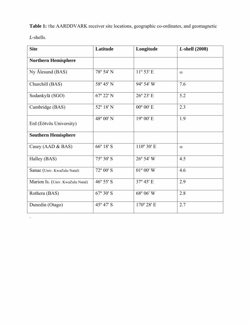
Table 1: The AARDDVARK receiver site locations, geographic co-ordinates, and geomagnetic
L-shells.
Site Latitude Longitude L-shell (2008)
Northern Hemisphere
Ny Ålesund (BAS) 78º 54' N 11º 53' E ∞
Churchill (BAS) 58º 45' N 94º 54' W 7.6
Sodankylä (SGO) 67º 22' N 26º 23' E 5.2
Cambridge (BAS) 52º 18' N 00º 00' E 2.3
Erd (Eötvös University) 48º 00' N 19º 00' E 1.9
Southern Hemisphere
Casey (AAD & BAS) 66º 18' S 110º 30' E ∞
Halley (BAS) 75º 30' S 26º 54' W 4.5
Sanae (Univ. KwaZulu Natal) 72º 00' S 01º 00' W 4.6
Marion Is. (Univ. KwaZulu Natal) 46º 55' S 37º 45' E 2.9
Rothera (BAS) 67º 30' S 68º 06' W 2.8
Dunedin (Otago) 45º 47' S 170º 28' E 2.7
.

Table 2: VLF transmitter call signs, frequency, geographic co-ordinates, output power, and
geomagnetic L-shells.
Transmitter ID Frequency
(kHz)
Latitude Longitude Power (kW)
estimated
L-shell
(2008)
NRK, Iceland 37.5 63º 51' N 22º 28' W 100 5.5
NLK, Seattle 24.8 48º 12' N 121º 55' W 250 2.9
NDK, N.Dakota 25.2 46º 22' N 98º 20' W 500 3.3
NAA, Maine 24.0 44º 39' N 67º 17' W 1000 2.9
GQD, Anthorn 22.1 54º 53' N 03º 17' W 60 2.7
HWU, Rosnay 22.6 46º 43' N 01º 15' E 200 1.8
DHO, Ramsloh 23.4 53º 05' N 07º 37' E 300 2.4
ICV, Tavolara Is. 20.27 40º 55' N 09º 45' E 50 1.5
NWC, N.W.Cape 19.8 21º 49' S 114º 10' E 1000 1.4
NTS, Woodside 18.6 38º 29' S 146º 56' E 25 2.4
NPM, Hawaii 21.4 21º 26' N 158º 09' W 500 1.2
NAU, Puerto Rico 40.75 18º 25' N 67º 09' W 125 -
JAP, Ebino 22.2 32º 03' N 130º 50' E 100 1.2

Figures
Figure 1. Schematic of subionospheric VLF propagation. The vast majority of the
energy in VLF transmissions propagate in the waveguide formed by the Earth and
the lower edge of the ionosphere (for night time ~85 km).
Figure 2. The great circle paths between the monitored VLF communications
transmitters (Tx, circles) and the existing AARDDVARK receiver locations (Rx, red
diamonds) are shown, indicating the atmospheric areas monitored. Our planned
AARDDVARK sensors for the future are shown as yellow squares.
Figure 3. The AARDDVARK great circle plot maps for the northern and southern
polar regions, viewed with L-shell contours at 3, 4, 6. Note some of the paths are
quasi-constant in L-shell.
Figure 4. Showing the variability of solar proton fluxes >50 MeV during the
October/November 2003 Halloween storms, the effects of the solar proton
precipitation on the ionization rate at ~73 km, and on the radio wave amplitude of the
VLF transmitter in Seattle (NLK) received in Ny Ålesund, Svalbard, Norway. The
lowest panel shows the percentage decreases of polar Ozone at ~73 km during the
same solar proton event, calculated using the Sodankylä Ion Chemistry model.
Figure 5. Showing the effects of energetic electron precipitation, during a
magnetospheric shock event driven by a coronal mass ejection, on radio wave
amplitudes received at Sodankylä, Finland (L=5). Both short and long time-scale
amplitude perturbations (i.e., particle precipitation) signatures are observed.
Figure 6. Winter time AARDDVARK data from Ny Ålesund, Svalbard using the
Iceland transmitter (NRK, 37.5 kHz) taken over 5 years. The radio wave index is
shown, representing the amplitude difference between average midday and midnight
propagation conditions, with solid vertical lines representing times of changed
ionization conditions due to solar proton events (with the peak >10 MeV fluxes in
brackets), and the dashed vertical lines representing ionization changes caused by the
descent of odd nitrogen (NOX) from the thermosphere.
Figure 7. Example of a sequence of solar flares on 02 December 2005 observed at
Casey, Antarctica on three separate paths from Australia and Japan, shown in
amplitude along with the co-incident GOES 0.1-0.8 nm X-ray fluxes and flare
classifications.

Figure 1. Schematic of subionospheric VLF propagation. The vast majority of the
energy in VLF transmissions propagate in the waveguide formed by the Earth and
the lower edge of the ionosphere (for night time ~85 km).
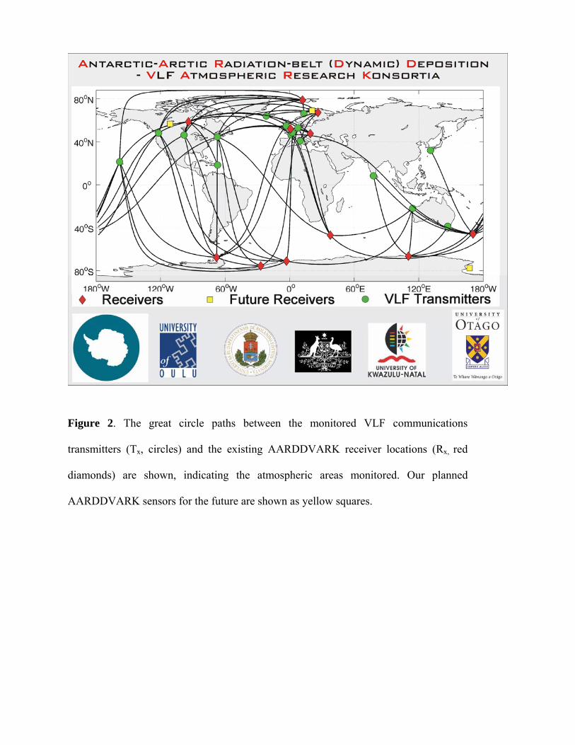
Figure 2. The great circle paths between the monitored VLF communications
transmitters (Tx, circles) and the existing AARDDVARK receiver locations (Rx, red
diamonds) are shown, indicating the atmospheric areas monitored. Our planned
AARDDVARK sensors for the future are shown as yellow squares.

Figure 3. The AARDDVARK great circle plot maps for the northern and southern
polar regions, viewed with L-shell contours at 3, 4, 6. Note some of the paths are
quasi-constant in L-shell.

Figure 4. Showing the variability of solar proton fluxes >50 MeV during the
October/November 2003 Halloween storms, the effects of the solar proton precipitation on the
ionization rate at ~73 km, and on the radio wave amplitude of the VLF transmitter in Seattle
(NLK) received in Ny Ålesund, Svalbard, Norway. The lowest panel shows the percentage
decreases of polar Ozone at ~73 km during the same solar proton event, calculated using the
Sodankylä Ion Chemistry model.

Figure 5. Showing the effects of energetic electron precipitation, during a
magnetospheric shock event driven by a coronal mass ejection, on radio wave
amplitudes received at Sodankylä, Finland (L=5). Both short and long time-scale
amplitude perturbations (i.e., particle precipitation) signatures are observed.

Figure 6. Winter time AARDDVARK data from Ny Ålesund, Svalbard using the
Iceland transmitter (NRK, 37.5 kHz) taken over 5 years. The radio wave index is
shown, representing the amplitude difference between average midday and midnight
propagation conditions, with solid vertical lines representing times of changed
ionization conditions due to solar proton events (with the peak >10 MeV fluxes in
brackets), and the dashed vertical lines representing ionization changes caused by the
descent of odd nitrogen (NOX) from the thermosphere.

Figure 7. Example of a sequence of solar flares on 02 December 2005 observed at
Casey, Antarctica on three separate paths from Australia and Japan, shown in
amplitude along with the co-incident GOES 0.1-0.8 nm X-ray fluxes and flare
classifications.