Remote Sensing of Environment 115 (2011) 2652–2663

Contents lists available at ScienceDirect

Remote Sensing of Environment

j ourna l homepage: www.e lsev ie r.com/ locate / rse

Persistent Scatterer InSAR: A comparison of methodologies based on a model oftemporal deformation vs. spatial correlation selection criteria

Joaquim J. Sousa a,b,⁎, Andrew J. Hooper c, Ramon F. Hanssen c, Luisa C. Bastos d,e, Antonio M. Ruiz e,f

a Escola de Ciências e Tecnologia, Universidade de Trás-os-Montes e Alto Douro, Vila Real, Portugalb Centro de Geologia da Universidade do Porto, Portugalc Institute of Earth Observation and Space Systems, Delft University of Technology, Delft, The Netherlandsd Observatório Astronómico, Faculdade de Ciência da Universidade do Porto, Portugale Department of Geosciences, Environment and Spatial Planning, Faculty of Science, University of Porto, Portugalf Departamento de Ingeniería Cartográfica, Geodésica y Fotogrametría, Universidad de Jaén, Jaén, Spain

⁎ Corresponding author at: Quinta de Prados ApartaPortugal. Fax: +351 259350356.

E-mail addresses: jjsousa@utad.pt, jjmsousa@gmail.c

0034-4257/$ – see front matter © 2011 Elsevier Inc. Aldoi:10.1016/j.rse.2011.05.021

a b s t r a c t

a r t i c l e i n f o

Article history:Received 5 December 2010Received in revised form 29 May 2011Accepted 29 May 2011Available online 17 June 2011

Keywords:PSIDeformationDePSIStaMPS

In this paper, two Persistent Scatterer Interferometry (PSI) methodologies are compared in order to furtherunderstand their potential in the detection of surface deformation. A comparison of these two algorithms is acomparison of the two classes of PSI techniques available: coherence estimation based on a temporal model ofdeformation (represented by DePSI) and coherence estimation based on spatial correlation (represented byStaMPS).Despite the similarity between the results obtained from the application of the two independent PSImethodologies, significant differences in PS density and distribution were detected, motivating a comparativestudy between both techniques. We analyze which approach might be more appropriate for studying specificareas/environments, which is helpful in evaluating the benefits that could be derived from an integration ofthe two methodologies. Several experiments are performed to assess the sensitivity of both PSI approaches todifferent parameter settings and circumstances. The most significant differences in the processing chain ofboth procedures are then investigated. We apply both methodologies to the Granada Basin area (southernSpain) and realize that coherence does not improve significantly as function of the methodology applied. Ifoversampling is implemented in the StaMPS processing chain, the PS density increases so that the density inthe urbanized areas is similar to the results provided by DePSI but in all the remaining covers the density issignificantly higher. The general results provided by both approaches are very similar in the relativedeformations estimated.

do 1013, 5001-801 Vila Real,

om (J.J. Sousa).

l rights reserved.

© 2011 Elsevier Inc. All rights reserved.

1. Introduction

Radar interferometry (InSAR) has matured to become a widely usedgeodetic technique for measuring deformation of the Earth's surface.There are two main characteristics which make this technique attractiveto the scientific community. The first is that it gives a high resolution two-dimensional representation of the deformation over 10s to 100s ofkilometers. The second is the high accuracy of the deformation that can bemeasured. The accuracy depends chiefly on variation in atmosphericconditions; the variable water vapor distribution related to the turbulentcharacter of the atmosphere creates an interferometric phase contribution(Hanssen, 2001). For single interferograms, this atmospheric phase screen(APS) cannot easily be removed and therefore the accuracy of measuringsmall deformations is significantly reduced. The challenge is to separatethe desired signal from the sum of all contributions to the phase. For

terrain displacement studies, temporal decorrelation can be considered arandom noise source while errors in the digital elevation model (DEM)used to remove the topographic phase, orbital errors, and atmosphericchanges will introduce a spatially systematic phase trend.

Until recently, a large proportion of InSAR application results wereachieved by analyzing single interferograms derived from a single pairof SAR images. In the late 1990s it was noted that some radar targetsmaintain stable backscattering characteristics for a period of monthsor years or even decades (Usai, 1997; Usai & Hanssen, 1997). Thisprovided the basis for further exploitation of existing SAR scenearchives using Multi-temporal InSAR techniques (MT-InSAR), involv-ing the processing of multiple acquisitions in time, to overcomeconventional InSAR limitations: temporal and geometric decorrela-tion, and atmospheric inhomogeneities (Ferretti et al., 1999, 2001).The main concept behind PSI technique lies on the identification ofsingle targets (called Persistent Scatterers, PS) that are coherent overlong time intervals and for wide look-angle variations (Ferretti et al.,2000, 2001). The signal received for these targets varies little as theother scatterers move around, and any motion of the scatterer can be

Table 2ERS data for the Granada Basin area (track 280; frame 2859). Parameters are relative tothe master acquisition, orbit 11657, acquired on 13-JUL-1997 10:56 AM (UTC).

# Acq. date Orbit Sensor B⊥(m) fdc(Hz)

1 02-DEC-1993 12449 ERS1 920 3852 03-JUN-1995 20308 ERS1 134 4053 04-APR-1999 20675 ERS2 211 1374 04-MAY-1997 10655 ERS2 −225 1265 06-AUG-2000 27689 ERS2 269 −3726 06-SEP-1998 17669 ERS2 180 1537 08-FEB-1998 14663 ERS2 −141 1098 09-JAN-2000 24683 ERS2 −36 1639 12-AUG-1995 21310 ERS1 270 40310 13-AUG-1995 1637 ERS2 208 12011 13-JUL-1997 11657 ERS2 0 12312 13-JUN-1999 21677 ERS2 −460 16513 15-DEC-1996 8651 ERS2 −179 18914 15-OCT-2000 28691 ERS2 583 −6215 17-JUL-1999 41851 ERS1 811 40716 18-MAY-1996 25318 ERS1 279 37817 19-MAY-1996 5645 ERS2 198 13518 21-AUG-1999 42352 ERS1 1446 40819 21-OCT-1995 22312 ERS1 902 33120 22-AUG-1999 22679 ERS2 1140 17321 22-OCT-1995 2639 ERS2 1031 9522 24-DEC-2000 29693 ERS2 −325 −5223 25-MAR-1995 19306 ERS1 −1040 384

2653J.J. Sousa et al. / Remote Sensing of Environment 115 (2011) 2652–2663

readily measured by the phase of the radar echo. In fact, when thedimension of the PS is smaller than the resolution cell, the coherenceis good even for image pairs taken with baselines greater than thedecorrelation length. On those pixels, sub-meter DEM accuracy andmillimetric terrain motion detection can be achieved (see e.g.Ketelaar, 2008; Hooper, 2006), even if the coherence is low in thesurrounding areas. Reliable elevation and deformation measurementscan, then, be obtained on this subset of image pixels that can be usedas a ‘natural geodetic network’.

In this paper we compare two persistent scatterer methodsrepresenting the two different approaches: those that select pixelsbased mainly on their phase variation in time (e.g., Ferretti et al.,2001; Kampes, 2005; Ketelaar, 2008) and those that use mainlycorrelation of their phase in space (Hooper et al., 2004; van der Kooijet al., 2006). We apply DePSI (Delft PSI processing package),belonging to the former group and StaMPS (Stanford Method forPersistent Scatterers), belonging to the last group, to the same dataset. Detailed descriptions of these two PSI methodologies can be foundin Hooper et al. (2007), Kampes (2005), Ketelaar (2008), and Sousa(2009). Both PSI methodologies provide broadly similar results (Sousaet al., 2010a); however there are some differences, mainly concerningPS density and location. In this work we investigate all the significantdifferences between both implementations.

24 28-JUN-1998 16667 ERS2 −703 15825 28-MAY-2000 26687 ERS2 923 −28526 30-MAR-1997 10154 ERS2 409 14827 30-OCT-1999 43354 ERS1 805 40428 31-DEC-1995 3641 ERS2 313 17029 31-OCT-1999 23681 ERS2 485 88

2. Setting of the study area

The study area, the Granada Basin and its surroundings, is locatedin southern Spain around the western and southern flanks of SierraNevada. From a geological standpoint, these zones are part of theAlpujárride and Nevado–Filábride complexes within the Internal Zoneof the Betic Cordillera, which are filled with postorogenic deposits ofNeogene to Quaternary age. The region was formed during the Alpineorogeny and is affected by a complex geologic evolution (Galindo-Zaldívar et al., 1993; Sanz de Galdeano & Vera, 1992). The Granadabasin occupies the central sector of the Betic Cordillera, one of themost seismically-active areas in the Iberian Peninsula, accompaniedby significant active tectonics. Granada is the most populated city ofthe central Betic Cordillera.

Table 3Envisat data for the Granada Basin area (track 187; frame 737). Parameters are relativeto the master acquisition, orbit 10261, acquired on 15-FEB-2004 10:01 PM (UTC).

# Acq. date Orbit Sensor B⊥(m) fdc(Hz)

1 13-OCT-2002 3247 ASAR −104 −5552 17-NOV-2002 3748 ASAR −402 −5683 11-MAY-2003 6253 ASAR 607 −4204 20-JUL-2003 7255 ASAR −62 −4865 24-AUG-2003 7756 ASAR −59 −5746 28-SEP-2003 8257 ASAR 1041 −5937 07-DEC-2003 9259 ASAR 194 −5688 11-JAN-2004 9760 ASAR 280 −5389 15-FEB-2004 10261 ASAR 0 −540

3. Satellite datasets

This work is based on a set of ERS-1/2 and Envisat SAR images fromdescending and ascending satellite tracks, covering the period fromDecember 1993 to July 2006. In the case of ERS acquisitions, only thescenes acquired until the end of 2000 have been included in theprocessing in order to avoid high Doppler values due to the failures ofthe ERS-2 gyroscopes.

The ERS and Envisat tracks that cover the Granada Basin area arelisted in Table. 1. Each track has been processed using interferometriccombinations that refer to a common master. The master sceneacquisitions have been selected based on stack coherence (seeSection 5.1). Tables 2 and 3 indicate the sets of ERS and Envisatimages used in this project. Each image covers 100 by 100 km2.

Table 1The four ERS/Envisat tracks that cover the Granada Basin area. The master has beenselected based on stack coherence.

Sensor Track Frame Mode No. scenes Master

ERS 280 2859 Dec 29 13.07.1997ERS 187 737 Asc 6 *Envisat 280 2859 Desc 17 *Envisat 187 737 Asc 22 15.02.2004

* Number of scenes insufficient for PSI processing.

The number of interferograms is limited to 28 for ERS data and 21for Envisat data. All 28 ERS interferograms are generated with amaster image, acquired on 17 July, 1997 while Envisat interferogramsare generated with a master image acquired on 15 February, 2004.

4. Mathematical modeling

Observed interferometric phase measurements are affected by theimaging geometry, topography, atmospheric propagation and scat-terer displacement or deformation. In time-series InSAR, we deal withthe problem of estimating a time-series of surface deformation from aseries of interferograms. Hence, the interferometric phase of a pixel

10 25-APR-2004 11263 ASAR −256 −53211 04-JUL-2004 12265 ASAR 634 −54512 08-AUG-2004 12766 ASAR 568 −57313 12-SEP-2004 13267 ASAR 200 −54314 17-OCT-2004 13768 ASAR −849 −54415 30-JAN-2005 15271 ASAR −51 −54116 10-APR-2005 16273 ASAR −318 −55317 15-MAY-2005 16774 ASAR −164 −54018 28-AUG-2005 18277 ASAR 388 −55019 06-NOV-2005 19279 ASAR −225 −51320 19-FEB-2006 20782 ASAR 660 −52021 26-MAR-2006 21283 ASAR 1027 −50822 09-JUL-2006 22786 ASAR −886 −507

2654 J.J. Sousa et al. / Remote Sensing of Environment 115 (2011) 2652–2663

(φint) in a differential interferogram can be represented by (Hooperet al., 2007):

φint = φdefo + Δφε + Δφatm + Δφorb + φn ð1Þ

whereφdefo represents the phase due to deformation, Δφε refers to theerror introduced by using imprecise topographic information, φorb

refers to the error introduced due to the use of imprecise orbits inmapping the contributions of Earth's ellipsoidal surface, φatm

corresponds to the difference in atmospheric propagation timesbetween the two acquisition used to form the interferogram and φn

represents the phase noise due to the scattering background andother uncorrelated noise terms.

In PSI, our primary signal of interest is the return from thedominant scatterer in the resolution element. The echoes from thedimmer distributed scatterers in a pixel is also commonly referred toas “clutter” and contributes toφn. Signal-to-clutter ratio (SCR) definedas the ratio between the reflected energy from the dominant scattererto that of the reflected energy from the rest of the resolution elementis a measure often used to indicate the strength of the dominantscatterer in SAR pixels. High SCR (N8) pixels exhibit low interfero-metric phase variation (b0.25 rad) and vice versa.

PSI frameworks are a collection of spatial and temporal filteringroutines that allow us to estimate each of the phase componentsrepresented in Eq. (1) by assuming a spectral structure. Section 5.2describes the two methods used in this work.

5. Methods

5.1. Interferometric processing

Both PSI procedures used in this study make use of Delft Object-oriented Radar Interferometric Software (DORIS) (Kampes & Usai,1999) for the interferometric processing. The key steps of interfero-metric processing summarized in section 1 of Figs. 1 and 2 areexplained in the next sub-sections.

5.1.1. Master selectionA stack of differential interferograms coregistered to a selected

master scene is the input to the PSI processing in both approaches. ForN+1 SAR acquisitions, N independent interferometric combinationsbetween two images can be formed. The master is selected in such away to maximize the (predicted) total coherence of the interfero-metric stack, based on the perpendicular baseline, temporal baseline,and the mean Doppler centroid frequency difference (Zebker &Villasenor, 1992). In short, the master scene is chosen from theavailable SAR images on the basis of favorable geometry related to allother images, high coherence and possibly minimum atmosphericdisturbances.

5.1.2. Oversampling and coregistrationIn DePSI, after reading the SLC scenes, the SAR images are

oversampled by a factor of 2 (both range and azimuth directions)before the coregistration. This step is performed to avoid aliasing inthe complex multiplication of the SAR images.

The oversampled images and the precise orbits (Doornbos &Scharro, 2004; Scharroo & Visser, 1998) are the input for thecoregistration of the master and the slave image. This step isfundamental in interferogram generation, as it ensures that eachground target contributes to the same (range, azimuth) pixel in boththe master and the slave image. For the estimation of an accuratecoregistration polynomial, the coregistration windows are evenlydistributed over the area of interest. Especially in rural areas that areaffected by temporal decorrelation, a proper choice of coregistrationwindows is required.

In StaMPS oversampling is not applied and the coregistrationprocedure is also different. In order to avoid decorrelation problems inthe case of large temporal and spatial baselines, offsets in position areestimated for each coregistration window between pairs of imageswith good correlation. The function that maps the master image toeach other image is then estimated by weighted least-squaresinversion (Hooper et al., 2007).

In both procedures, once the mapping functions are estimated,each image is resampled to the master coordinate system, using a 12point raised cosine interpolation kernel. Then a raw interferogram isformed by differentiating the phase of each image to the phase of themaster.

5.1.3. Differential interferogram computationThe interferogram is computed by complex multiplication of the

master image and the resampled slave image observations. Areference Digital Elevation Model (DEM) and precise orbits data areused as input to obtain the differential interferograms. The interfero-metric phase component that is induced by topography is largelyeliminated using the differential technique, see, e.g. (Bamler & Hartl,1998; Burgmann et al., 2000). After the Shuttle Radar TopographyMission (SRTM), a DEM of sufficient precision is readily available forpractically any area of the world between −57° and 60° latitude(Suchandt et al., 2001).

5.2. PS processing

5.2.1. DePSITo initiate the DePSI algorithm, a first set of PS candidates (PSC) is

selected (Fig. 1). These PSs should preferably have stable phasebehavior in time. Because the observed wrapped interferometricphases do not enable the identification of stable points, and thecomputational limitations due to the initial high amount of pixels tobe tested, approximation methods are used. One option is to use thescatterer's intensity as a proxy. Although it is the phase stability of apixel that defines a PS pixel, there is a statistical relationship betweenamplitude stability and phase stability, which makes consideration ofamplitude useful for reducing the initial number of pixels for phaseanalysis. The amplitude dispersion index is defined by Ferretti et al.(2001) as:

DA =σA

μA≅σφ ð2Þ

where σA and μA are, respectively, the standard deviation and themean of a series of amplitude values. Ferretti et al. (2001) show thatfor a constant signal and high signal to noise ratio (SNR), DA≈σφ,where σφ is the phase standard deviation. Nevertheless, prior to thisinitial selection, a digital elevation model (DEM) will be used toremove most of the topographic phase signature from the interfero-grams. A network is formed between the selected PSC, which enablecalculation of the topographic height and displacement of a PS perepoch relative to a chosen reference point (RP). Various models maybe used (Leijen & Hanssen, 2007). However the application of aspecific model should be tuned to a priori knowledge about thedeformation development in space and time. Without any a prioriknowledge about deformation, a linear deformation mechanism isusually assumed. First, the parameters of interest and ambiguities areestimated for the arcs using Integer Least Square approach. Theseparameters can then be spatially unwrapped, with respect to anarbitrary RP, if possible, located in a stable area. PSC that can be testedor experience ambiguities not fitting in the unwrapped network arerejected as PS and not taken into account in further processing steps. Asmaller set of PS remains to which filters are applied for the sepa-ration of atmospheric phase. The atmospheric phase screen (APS)of the interferogram is computed using a geostatistical interpolation

Fig. 1. Flow diagram of the DePSI processing chain.

2655J.J. Sousa et al. / Remote Sensing of Environment 115 (2011) 2652–2663

method, which is sequentially subtracted from differential phase ofthe PSC. Processing steps starting from forming the network untilspatial unwrapping the arcs will be performed, again using the phasescorrected for the atmosphere.

Finally (section 3 of Fig. 1) after the subtraction of the atmosphericphase contribution estimated from the first order network, a furtherdensification step is performed by the analysis of the phase history ofPSC with a lower normalized amplitude dispersion. Parameter estima-tion is performed for each candidate (now called PS Potential — PSP)

with respect to the three closest accepted PS (belonged to the 1st ordernetwork). Again, these PSP are checked on their consistency. When atleast two of the three estimated arcs are in agreement, the PSP is storedas PS. After ambiguity and parameter estimation per arc, the parametersof interests are relative in space. So, they should be spatially integratedwith respect to a single reference point (reference PS) in order to obtainabsolute values. Due to noise andmodel imperfections, residuals will bepresent after integration. The unwrapping errors can be identified andrejected using the spatial network. Arcs with a questionable precision

Fig. 2. Flow diagram of the StaMPS processing chain.

2656 J.J. Sousa et al. / Remote Sensing of Environment 115 (2011) 2652–2663

are rejected. This precision can be deduced from, e.g., low temporalensemble coherence or large least-squares residues. Themeasure of thevariation of the residual phase for a pixel (x, y) is defined as:

γ̂x;y =1N

∑N

k=1e

j⋅φerrorx;y

� �ð3Þ

where γ̂ resembles the estimate of the ensemble coherence, N is thetotal amount of interferograms and j is the imaginary number. Theresidual, φerrorx, y, is the difference between the modeled and observedphases at location (x, y) in the observed interferogram.

Assuming that all ambiguities are estimated correctly, theintegration with respect to the RP can be carried out simply by pathintegration of temporally unwrapped phases without residues. The

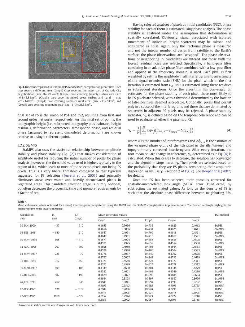
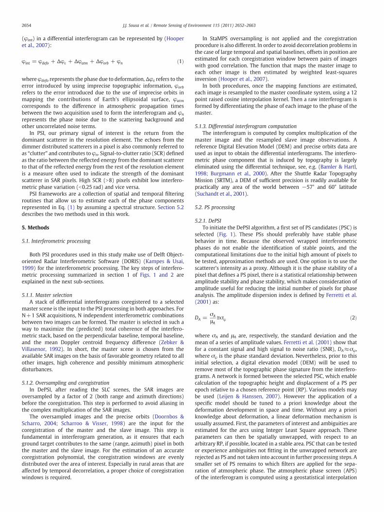
Fig. 3.Different crops used to test the DePSI and StaMPS coregistration procedures. Eachcrop covers a different area. (Crop1) Crop covering the major part of Granada Cityneighborhood (size 36×22 km2); (Crop2) crop covering (mainly) urban area (size~6.4×6.8 km2); (Crop3) crop covering mixed areas (urban and rural — size~23×14 km2); (Crop4) Crop covering (almost) rural areas (size ~13×9 km2) and(Crop5) crop covering mountain area (size ~11.3×21.3 km2).

2657J.J. Sousa et al. / Remote Sensing of Environment 115 (2011) 2652–2663

final set of PS is the union of PS1 and PS2, resulting from first andsecond order networks, respectively. For this final set of points, thetopographic height (i.e., subtracted topography plus estimated heightresidual), deformation parameters, atmospheric phase, and residualphase (assumed to represent unmodeled deformation) are knownrelative to a single reference point.

5.2.2. StaMPSStaMPS also uses the statistical relationship between amplitude

stability and phase stability (Eq. (2)) that makes consideration ofamplitude useful for reducing the initial number of pixels for phaseanalysis; however, the threshold value used is higher, typically in theregion of 0.4, which leads to most of the selected pixels not being PSpixels. This is a very liberal threshold compared to that typicallysuggested for PS selection (Ferretti et al., 2001) and primarilyeliminates areas over water and heavily decorrelated pixels invegetated areas. This candidate selection stage is purely optional,but often decreases the processing time andmemory requirements bya factor of ten.

Table 4Mean coherence values obtained for (some) interferogram coregistered using the DePSIinterferograms with lower coherence.

Acquisitiondate

B⊥(m)

ΔT(days)

Mean coherence values

Crop1 Crop

09-JAN-2000 −37 910 0.4655 0.5050.4656 0.505

08-FEB-1998 −140 210 0.4647 0.4950.4647 0.495

19-MAY-1996 198 −419 0.4571 0.4920.4571 0.492

13-AUG-1995 207 −700 0.4598 0.4980.4598 0.498

04-MAY-1997 −225 −70 0.4776 0.5050.4777 0.505

31-DEC-1995 312 −559 0.4371 0.4580.4372 0.458

30-MAR-1997 409 −105 0.4349 0.4600.4352 0.460

15-OCT-2000 582 1190 0.3679 0.3820.3684 0.382

28-JUN-1998 −702 349 0.3688 0.3840.3695 0.384

02-DEC-1993 919 −1319 0.2909 0.2800.2916 0.300

22-OCT-1995 1029 −629 0.2954 0.2940.2955 0.299

Characters in italics are the interferograms with lower coherence.

Having selected a subset of pixels as initial candidates (PSC), phasestability for each of them is estimated using phase analysis. The phasestability is analyzed under the assumption that deformation isspatially correlated. Obviously, signal associated with isolatedmovement of individual bright scatterers may be missed andconsidered as noise. Again, only the fractional phase is measuredand not the integer number of cycles from satellite to the Earth'ssurface: the phase observations are “wrapped”. The phase observa-tions of neighboring PS candidates are filtered and those with thelowest residual noise are selected. Specifically, a band-pass filterconsisting in an adaptive phase filter combined with a low-pass filterand applied in the frequency domain, is used. Each pixel is firstweighted by setting the amplitude in all interferograms to an estimateof the signal-to-noise ratio (SNR) for the pixel, which in the firstiteration is estimated from DA. SNR is estimated using these residuesin subsequent iterations. Once the algorithm has converged onestimates for the phase stability of each pixel, those most likely tobe PS pixels are selected, with a threshold determined by the fractionof false positives deemed acceptable. Optionally, pixels that persistonly in a subset of the interferograms and those that are dominated byscatterers in adjacent PS pixels may be rejected. A phase stabilityindicator, γx, is defined based on the temporal coherence and can beused to evaluate whether the pixel is a PS:

γx =1N j ∑N

i=1exp j φint;x;i−φ

int;x;i−Δφ̂h;x;i

� �n oj ð4Þ

where N is the number of interferograms and Δφ̂h;x;i is the estimate ofthe wrapped phase φint,x,i of the xth pixel in the ith flattened andtopographically corrected interferogram. After every iteration, theroot-mean-square change in coherence, γx, determined as in Eq. (4) iscalculated. When this ceases to decrease, the solution has convergedand the algorithm stops iterating. Then pixels are selected based onthe probability that they are PS pixels, considering their amplitudedispersion, as well as γx, (section 2 of Fig. 2). See Hooper et al.(2007)for details.

Once the PS has been selected, their phase is corrected forspatially-uncorrelated look angle (SULA) error (DEM error) bysubtracting the estimated values. As long as the density of PS issuch that the absolute phase difference between neighboring PSs,

and the StaMPS coregistration implementations. The dashed rectangle highlights the

PSI method

2 Crop3 Crop4 Crop5

6 0.4735 0.4625 0.4612 DePSI6 0.4734 0.4625 0.4611 StaMPS1 0.4709 0.4618 0.4591 DePSI1 0.4710 0.4617 0.4591 StaMPS4 0.4658 0.4555 0.4508 DePSI5 0.4658 0.4554 0.4508 StaMPS0 0.4705 0.4564 0.4533 DePSI0 0.4706 0.4564 0.4533 StaMPS7 0.4840 0.4792 0.4628 DePSI7 0.4841 0.4792 0.4629 StaMPS8 0.4424 0.4377 0.4311 DePSI9 0.4425 0.4378 0.4312 StaMPS0 0.4401 0.4348 0.4279 DePSI1 0.4403 0.4349 0.4280 StaMPS7 0.3696 0.3685 0.3654 DePSI8 0.3697 0.3687 0.3656 StaMPS1 0.3690 0.3599 0.3767 DePSI2 0.3692 0.3603 0.3765 StaMPS6 0.2828 0.2790 0.3103 DePSI5 0.2921 0.2918 0.3005 StaMPS4 0.2873 0.2724 0.3210 DePSI2 0.2967 0.2905 0.3118 StaMPS

Fig. 4. Graphic representation of the coherence values listed in Table. 4 as a function of the perpendicular baseline. The mean coherence decreases when B∞ increases. As expected,urban areas present the higher value of mean coherence and the mountainous areas the lowest regardless of the method applied.

2658 J.J. Sousa et al. / Remote Sensing of Environment 115 (2011) 2652–2663

after correction for estimated SULA error, is generally less than π, thecorrected phase values can now be unwrapped.

The first “interpretable” PSI observation is the double-differencebetween master and slave for two nearby PS (Hanssen, 2004). Thedouble-difference is both a temporal and a spatial difference. Thisimplies that StaMPS also requires a spatial and a temporal reference:one acquisition time (master image) and one reference PS or ref-erence area.

Optionally, after unwrapping, high-pass filtering can be applied tounwrapped data in time followed by a low-pass filter in space in orderto remove the remaining spatial correlated errors (atmosphere andorbit errors).

Finally, subtracting this signal leaves essentially deformation andspatially uncorrelated errorswhich can bemodeled as noise (section 3of Fig. 2). All the remaining noise terms are supposed to be sub-stantially reduced.

Fig. 5. StaMPS processing. (a) Without oversampling implementation; (b) with oversamdeformation rates match it is clear that the amount of PS becomes much higher when over

6. Comparative study

The main conceptual difference between DePSI and StaMPS lies inthe deformation assumption. In DePSI pixels are selected based on themodel of the temporal behavior while in StaMPS spatial smoothness ofthe deformation signal is assumed for PS selection. This can lead todifferent sets of PS being selectedby eachapproach (Sousa et al., 2010a).

In the next sections, the most significant differences between bothapproaches are evaluated following the processing chain diagramsrepresented in Figs. 1 and 2. The preliminary results can be found inSousa et al. (2010b).

6.1. Coregistration influence

In order to evaluate the influence of this step in both approaches,we computed the coherence between the master and the resampled

pling implementation (factor 2 in both azimuth and range directions). Although thesampling is implemented.

Table 5PS density as function of the soil occupation. Excluding the urbanized area whichdominates the processed area the remaining area is characterized by agriculture fieldswith scattered farms, small villages and mountains. Crop locations and sizes arepresented in Fig. 3.

PSI method PS density per crop

Crop1 Crop2 Crop3 Crop4 Crop5

DePSI 55 355 120 27 0.5StaMPS (no ovs) 18 55 23 10 12StaMPS (ovs) 108 295 148 71 87

Fig. 7. PS distribution over Otura village returned by: (a) DePSI and (b) StaMPS. SomePSs are selected in each image inside the subsidence bowl and their time series arerepresented in Fig. 8. A 0.5 m resolution ortophoto is used as a background.

2659J.J. Sousa et al. / Remote Sensing of Environment 115 (2011) 2652–2663

slave for different registration procedures. In other words, thecoherence theory for SAR interferograms is employed (Cattabeniet al., 1994; Just & Bamler, 1994) to predict the effect of interpolationon the interferogram phase quality. The average of the wholecoherence crop is used as criteria to evaluate the coregistrationresults of DePSI and StaMPS coregistration algorithms.

Wedivided the test area into different crops, coveringdistinct terrainoccupations and processed each crop separately. Fig. 3 shows somecrops used in the tests. As expected, the crops processed and presentedin Fig. 3 have significant differences in coherence values depending onthe type of the terrain they cover. The coherence along the mountainslopes is generally poor, mainly due to layover and shadow. Urban areaspresent high coherence due to the abundance of man-made construc-tions that behave as stable scatterers. The mean coherence values forsome of the InSAR interferograms tested are included in Table 4 bothusing DePSI and StaMPS coregistration algorithms. Loss of coherencecan be observed as function of the perpendicular baseline. For baselinesclose to1000 m(~critical baseline) and evenbigger, theurbanized areasappear with low coherence values. This effect is due to the geometricdecorrelation caused by different observation geometries. These effectsare confirmed in Fig. 4.

6.1.1. Discussion of the resultsBoth PSI approaches used in this work basically use the same

method to coregister the SAR images with only one nuance: to avoidhigh geometrical decorrelation (and a corresponding low coherence)StaMPS uses a coregistration algorithm that applies an amplitudebased method to estimate offsets in position between pairs of imageswith good correlation (only pairs with small perpendicular baselineare coregistered).

Fig. 6. ERS-1/2 stack PSI results of the whole area (corresponding to crop1— Fig. 3) using: (a)is indicated by the black asterisk. The areas marked with a small white box represent the h

In order to verify the influence of these different methods, severaltests have been performed and according to the main results obtained(see Table. 4) we can conclude that no significant difference betweenboth approaches exists. In fact, when interferometric pairs withperpendicular baselines smaller than ~500 m, are used, the averagecoherence values obtained by both methodologies in areas withdifferent varieties of coverage (urbanized, rural, and mountainous)are practically the same. For high perpendicular baseline values smalldifferences of mean coherence values can be found which confirmsbetter performance of StaMPS methodology.

DePSI; (b) StaMPS. Amean amplitude image is used as background. The reference pointighest deformation rates (Otura village) and are enlarged in Fig. 7.

2660 J.J. Sousa et al. / Remote Sensing of Environment 115 (2011) 2652–2663

In short, for this particular area, the coherence does not improvesignificantly as function of the methodology applied. This could beexplained by the fact that the mean coherence values are alwaysrelatively high regardless of the crop used. In someparticular cases, onlythe use of the StaMPSmethod allows the coregistration (Hooper, 2006).

Furthermore the processing time for the StaMPS coregistrationmethod can be substantially higher, depending on the number ofimages used. For instance, for the Granada dataset composed by 29scenes, 69 coregistrations are computed instead of the 28 required bythe standard coregistration routine. Therefore, the coregistrationmethodology used by StaMPS only brings some benefits if the studyarea suffers from significant decorrelation.

6.2. Oversampling influence

In order to evaluate the oversampling effect, the results suppliedby StaMPS processing with and without oversampling implementa-tion are presented and compared. We implemented several tests inorder to evaluate the oversampling influence on the final results. TheStaMPS procedure was first applied with no oversampling imple-mented and the results were compared with DePSI. Then theoversampling step was implemented in the StaMPS processingchain and the results were compared with those previously obtained.

As presented in Sousa et al. (2010a), the density and the location ofthe PS appear to be the most obvious differences between bothapproaches. This fact could be related to the deformation behavior.Here we assess whether the oversampling implementation could bealso a contributing factor.

Fig. 5 shows the results for the same area (Granada area, Spain)with and without oversampling implementation. The amount of PS is

Fig. 8. Displacement time series of the selected PS in Fig. 7 with respect to the reference poinPS-D by StaMPS. PS-A and PS-A’, and PS-B and PS-B’ are located in nearby positions respec

considerably higher when oversampling by a factor of 2 in bothazimuth and range is applied. In total, 7256 PSs were detectedwithoutoversampling compared to 44.189 PSs when oversampling isincluded. Apparently, oversampling results in 6 times more PSswhich can be very significant.

6.2.1. Discussion of the resultsThe average PS density in the area of interest depends on the PSI

methodology used.With DePSI the total area is covered by ~55 PS/km2.This compares to 18 PS/km2when the standard StaMPS configuration isused. However, if oversampling is implemented in the StaMPSprocessing this number increases to more than 100 PS/Km2. ThesePSs are not evenly distributed. The PS density varies from up to 0–10PS/km2 in the rural/mountain areas to over 100 PS/km2 in theurbanized areas (Table. 5). The picture is drastically different in thecase of StaMPS. In general, the PS density in urbanized areas is lowerthan it is in DePSI (standard processing); however, the density issignificantly increased in the rural and mountain areas, whichconstitutes the main advantage of StaMPS (See Table. 5). If over-sampling is implemented in the StaMPS processing chain, the PSdensity increases so that the density in the urbanized areas is similar tothe results provided byDePSI but in all the remaining covers the densityis significantly higher. Fig. 6 illustrates this effect more clearly. It is clearthat DePSI detects much fewer PS in the center of the subsidence bowl(Fig. 7a) when compared with StaMPS (Fig. 7b).

In Fig. 8, time series plots, for four PSs located inside thesubsidence area, are shown (position of the PS points given inFig. 7). DePSI PS time series are quite linear as expected due to thelinear assumption used. PS time series of the points only selected byStaMPS (PS-C and PS-D), despite the linear behavior shown, present a

t (represented in Fig. 6). PS-A and PS-B are returned by DePSI and PS-A’, PS-B’, PS-C andtively.

Table 6Line-of-Sight (LOS) displacement rates estimated with DePSI and StaMPS of the twocommon PS given in Fig. 7.

PS Latitude Longitude DePSI StaMPS velDePSI-velStaMPS

Vel(mm/yr)

Coh Vel(mm/yr)

Coh (mm/yr)

A 37°.08574 −3°.63459 −5.4 0.78 −6.0 0.71 +0.6B 37°.08676 −3°.61662 −5.4 0.79 −6.2 0.62 +0.8

2661J.J. Sousa et al. / Remote Sensing of Environment 115 (2011) 2652–2663

high level of noise. This may be the explanation to the fact that theywere not selected by DePSI.

The estimated displacement rates and the quality of the comparedPSs (A–A’ and B–B’) are listed in Table 6, for both DePSI and StaMPS.The bias between algorithms for both estimates may be partly due tothe fact that in DePSI, velocities are with respect to a specific PS,whereas in StaMPS they are with respect to all PSs within a specifiedradius (3 km in this case).

The increase in the PSnumber after oversampling is expectedmainlydue to dominant scatterers that are not located in the center of theoriginal resolution cell. However, these “new PSs” should be, in fact,influenced by the one in the adjacent pixel. A scatterer that is bright candominate pixels other than the pixel corresponding to its physicallocation. The error in look angle and squint angle due to the offset of thepixel from the physical location usually results in these pixels not beingselected as PS. However, the slight oversampling of the resolution cellscan cause pixels immediately adjacent to the PS pixel to be dominatedby the same scatterer where the error may be sufficiently small that thepixel appears stable. To avoid picking these pixels, we assume thatadjacent pixels selected as PS are due to the samedominant scatterer. Aswe expect the pixel that corresponds to the physical location to have thehighest SNR, for groups of adjacent stable pixels we select as the PS onlythe pixel with the highest value of coherence.

We specifically exclude pixels that could be dominated by thesame scatterer, by searching for clusters of adjacent pixels, andkeeping only the pixel with the highest coherence. When the data areoversampled, the window used for coherence computation is alsoincreased by a factor of two in both directions and oversamplingduring coregistration is reduced by a factor of 2 resulting in the samecoregistration accuracy.

Fig. 9 presents the overlapped histograms relative to the coherencevalues considering all PSs obtained with oversampling and only theextra PS obtained by resampling. There is not a significant degradationof the coherence, implying that the increase in the number of PS wasnot achieved due to the inclusion of PS with noisier phase.

Fig. 9. Coherence density distribution using all the PS obtained from the processing of the arpoints have been added to the selection (cohb0.4) however this number is negligible whe

The improvement in the PS location is another benefit expected byapplying oversampling because the radar coordinates of an over-sampled image are at sub-pixel level with respect to the originalsampling rate.

Motivated by these results, a similar test was realized (Arikanet al., 2010) in the West Anatolia area, Turkey. This region is rural andonly few PSs can be detected when StaMPS standard design is applied.However, when oversampling is implemented the results aresignificantly improved, 417 PSs were detected before applyingoversampling in the StaMPS processing chain against 2029 PSs afteroversampling implementation.

We propose two reasons why the number of PS would increase.First, in the case where a dominant scatterer is close to the edge of aresolution cell, its influence is downweighted by the appropriatevalue of a sync function centered on the middle of the cell. In aneighboring (overlapping) oversampled resolution cell, this scattererwould lie close to the center and hence have a higher weight, leadingto increased SNR. Second, when two dominant scatterers lie close toeach other they may both influence a resolution cell, which would notthen behave as a PS. Neighboring oversampled resolution cells may bedominated by only one of the scatterers leading them to behave as PS.

Fig. 10 shows a comparison of Mean LOS Velocity (MLV) forhomologous pixels (PS) selected by both methods. This picture allowsa quantitative comparison between PS motion (MLV [mm/yr])computed by means of DePSI and StaMPS. For assessment of thesimilarity between DePSI and StaMPS deformation velocities thecorrelation coefficient was computed and having been found thevalue of 0.8997, which indicates a strong correlation between bothmethodologies.

6.3. Influence of PS selection methodologies

In order to test the influence of the different approaches in the PSselection, we used a SAR dataset with particular characteristics. Acontrolled corner reflector experiment has been set up with levelingas an independent validation technique (Marinkovic et al., 2007).Since early 2003, during almost five years, the movements of fivecorner reflectors in the area near Delft University of Technology weremonitored using leveling and repeat-pass InSAR (ERS-2 and Envisat).

According to the way that DePSI selects PS, very bright points witha very stable phase in time located in an area undergoing slowdeformation will be selected as PS. But the question rises:Will StaMPSbe able to detect these points as PS?

In the first stage, when StaMPS selects PS candidates based onamplitude dispersion, these points will be selected as well due to its

ea related to Fig. 6. (left) Absolute histogram; (right) normalized histogram. Few noisyn compared to the quality of the majority of the new points.

Fig. 10. Comparison of mean LOS velocity for all homologous PSs in the area cor-responding to Fig. 6.

2662 J.J. Sousa et al. / Remote Sensing of Environment 115 (2011) 2652–2663

very stable phase response. Then, candidates are filtered in smallpatches to determine the spatially-correlated phase. This is aniterative procedure that estimates the phase noise of each candidatein every interferogram. Noisy pixels are downweighted in the filteringand iteration continues until convergence of phase noise estimates isachieved. According to this principle, the corner reflectors will bedetectable by StaMPS if there are candidate pixels in the surroundingpatch that maintain some coherence, and the difference in motionbetween the reflectors and the background is not too great. In thatcase these movements will be considered as noise. In Fig. 11, theresults provided by both approaches can be compared. The generalresults are very similar both in density and in the relative de-formations estimated. Same results and relative deformations are alsoderived inside the region of the corner reflectors.

Fig. 11. Linear velocities in the corner reflectors area provided by: (a) DePSI. A topographic ma SAR amplitude image. It is possible to check the similarity between the linear velocities.

7. Conclusion

We have investigated the most significant differences in theStaMPS and DePSI processing chains in order to depict the behavior ofeach PSI approach according to the area and to the deformationregime. Critical differences in the interferometric processing werestudied: SAR image coregistration and oversampling. It was confirmedthat StaMPS coregistration method has benefits; however, theseimprovements are not significant in the case where the study areamaintains a reasonable correlation, even if long perpendicularbaselines are used. Another significant difference in the interfero-metric processing regards the oversampling step. StaMPS, unlikeDePSI, does not includes this step in its standard design. The benefitsfrom the inclusion of the oversampling step in StaMPSwere evaluatedand the results demonstrated that significant improvements, mainlyin the PS density, are obtained. Because of this, oversampling has beenadded to StaMPS framework as default option in the latest release.

Secondly, the PS processing part of each methodology wasanalyzed and evaluated. We concluded that StaMPS and DePSI arecomplementary in different aspects like the case of PS selection andunwrapping which can be used to improve the results.

Despite these differences, some of them significant, the generaldeformation framework has been detected by both approaches whenapplied to different datasets.

The next step in the development of this project will be theintegration of the major advantages of both PSI approaches becausethe expected benefits will be considerable mainly in the areas whereman-made structures are scarce.

Acknowledgments

This research was supported by the European Space Agency (ESA)in the scope of 3858 and 3963 CAT-1 projects, the PR2006-0330,ESP2006-28463-E, CSD2006-00041, and AYA2010-15501 projectsfrom Ministerio de Educación y Ciencia (Spain), the RNM-149 andRNM-282 research groups of the Junta de Andalucía (Spain) andFundação para a Ciência e a Tecnologia (Portugal). The SRTM datawere provided by USGS/NASA.

ap is used as background (Marinkovic et al., 2007); (b) StaMPS results superimposed to

2663J.J. Sousa et al. / Remote Sensing of Environment 115 (2011) 2652–2663

References

Arikan, M., Hooper, A., & Hanssen, R. (2010). Radar time series analysis over westanatolia. : European Space Agency (Special Publication) ESA SP-677, 2010.

Bamler, R., & Hartl, P. (1998). Synthetic aperture radar interferometry. Inverse Problems,14, R1–R54.

Burgmann, R., Schmidt, D., Nadeau, R. M., d'Alessio, M., Fielding, E. J., Manaker, D., et al.(2000). Earthquake potential along the Northern Hayward Fault, California. Science,289, 1178–1182.

Cattabeni, M., Monti-Guarnieri, A., & Rocca, F. (1994). Estimation and improvement ofcoherence in SAR interferograms. Proceedings of IGARSS 94, Pasadena, California.

Doornbos, E., & Scharro, R. (2004). Improved ERS and Envisat precise orbit determination.Proceedings of ERS/Envisat Symposium Saltzburg 2004. The orbit files are available athttp://www.deos.tudelft.nl/ers/precorbs/orbits/

Ferretti, A., Prati, C., & Roca, F. (1999). Multibaseline InSAR DEM reconstruction: Thewavelet approach. IEEE Transactions on Geoscience and Remote Sensing, 37(2),705–715.

Ferretti, A., Prati, C., & Rocca, F. (2000). Nonlinear subsidence rate estimation usingpermanent scatters in differential SAR interferometry. IEEE Transactions onGeoscience and Remote Sensing, 38(5), 2202–2212.

Ferretti, A., Prati, C., & Rocca, F. (2001). Permanent scatters in SAR interferometry. IEEETransactions on Geoscience and Remote Sensing, 39(1), 8–20.

Galindo-Zaldívar, J., González-Lodeiro, F., & Jabaloy, A. (1993). Stress and palaeostressin the Betic-Rif cordilleras (Miocene to the present). Tectonophysics, 227, 105–126.

Hanssen, R. F. (2001). Radar interferometry: Data interpretation and error analysis.Dordrecht: Kluwer Academic Publishers 2001.

Hanssen, R. F. (2004). Stochastic modeling of times series radar interferometry.International Geoscience and Remote Sensing Symposium, Anchorage, Alaska, 20–24September 2004.

Hooper, A. (2006). Persistent Scaterrer Radar Interferometry for Crustal DeformationStudies and Modeling of Volcanic Deformation. PhD thesis.

Hooper, A., Segall, P., & Zebker, H. (2007). Persistent scatterer InSAR for crustaldeformation analysis, with application to Volcán Alcedo, Galapagos. Journal ofGephysical Research, 112, B07407. doi:10.1029/2006JB004763.

Hooper, A., Zebker, H., Segall, P., & Kampes, B. (2004). A new method for measuringdeformation on volcanoes and other natural terrains using InSAR persistentscatterers. Geophysical Research Letters, 31, L23611. doi:10.1029/2004GL021737,2004.

Just, D., & Bamler, R. (1994). Phase statistics of interferograms with applications tosynthetic aperture radar. Applied Optics, 33(20), 4361–4368.

Kampes, B. M. (2005). Radar interferometry: Persistent scatterer technique. Dordrecht,The Netherlands: Kluwer Academic Publishers.

Kampes, B. M., & Usai, S. (1999). Doris: the Delft Object-oriented radar interferometricsoftware, 2nd International Symposium on Operationalization of Remote Sensing.The Netherlands: Enschede.

Ketelaar, V.B.H., 2008. Monitoring surface deformation induced by hydrocarbonproduction using satellite radar interferometry. PhD thesis, Delft University ofTechnology, Delft, The Netherlands.

Leijen, F. J. V., & Hanssen, R. F. (2007). Persistent Scatterer interferometry using adaptivedeformation models. ESA ENVISAT Symposium, Montreux, Switzerland, 23–27 April2007 6 pp., CD-ROM ESA SP-636.

Marinkovic, P., Ketelaar, G., van Leijen, F., & Hanssen, R. (2007). InSAR quality control:Analysis of five years of corner reflectors time series. Fringe Workshop 2007.Frascati, 26–30 November 2007, Italy.

Sanz de Galdeano, C., & Vera, J. A. (1992). Stratigraphic record and palaeogeographicalcontext of the Neogene basins in the Betic Cordillera. Spain Basin Research, 4, 21–36.

Scharroo, R., &Visser, P. (1998). Precise orbit determinationandgravityfield improvementfor the ERS satellites. Journal of Geophysical Research, 103(C4), 8113–8127.

Sousa, J.J. (2009). Potential of Integrating PSI Methodologies in the Detection of SurfaceDeformation. PhD Thesis, University of Porto, Portugal.

Sousa, J. J., Hooper, A., Hanssen, R. F., & Bastos, L. (2010). Comparative study of twodifferent PS-InSAR approaches: DePSI vs. StaMPS. Proceedings of FRINGE 2009Workshop, Frascati, 2009.

Sousa, J. J., Ruiz, A.M., Hanssen, R. F., Bastos, L., Gil, A., Galindo-Zaldívar, J., et al. (2010). PSIprocessing methodologies in the detection of field surface deformation—Study of theGranada basin (Central Betic Cordilleras, southern Spain). Journal of Geodynamics. doi:10.1016/j.jog.2009.12.002.

Suchandt, S., Breit, H., Adam, N., Eineder, M., Schättler, B., Runge, H., et al. (2001). Theshuttle radar topography mission. High Resolution Mapping from Space 2001,Hannover, 2001. Joint Workshop of ISPRS Working Groups I/2, I/5 and IV/7. Hannover:ISPRS, 2001 (pp. 235–242). 1 CD-ROM.

Usai, S. (1997). The use of man-made features for long time scale INSAR. Geoscienceand Remote Sensing, 1997. IGARSS '97. Remote sensing — A scientific vision forsustainable development, 1997. IEEE International, 4. (pp. 1542–1544).

Usai, S., & Hanssen, R. (1997). Long time scale INSAR by means of high coherencefeatures. 3rd ERS Symposium on Space at the service of our Environment, Florence,Italy, 14–21 March, European Space Agency.

van der Kooij, M., Hughes, W., Sato, S., & Poncos, V. (2006). Coherent target monitoringat high spatial density: Examples of validation results. Eur. Space Agency Spec. Publ.,SP-610.

Zebker, H. A., & Villasenor, J. (1992). Decorrelation in interferometric radar echoes. IEEETransactions on Geoscience and Remote Sensing, 30(5), 950–959.