Remote Sensing, Climate and GIS Data Analysis · Remote Sensing, Climate and GIS Data Analysis Jay...
59
Remote Sensing, Climate and GIS Data Analysis Jay Angerer MOR2 Annual Meeting June 2013
Transcript of Remote Sensing, Climate and GIS Data Analysis · Remote Sensing, Climate and GIS Data Analysis Jay...

Remote Sensing, Climate and
GIS Data Analysis
Jay Angerer MOR2 Annual Meeting
June 2013
Remote Sensing • The term "remote sensing," first used in the United
States in the 1950s by Ms. Evelyn Pruitt of the U.S. Office of Naval Research
• Defined as the science—and art—of identifying, observing, and measuring an object without coming into direct contact with it.
• Involves the detection and measurement of radiation of different wavelengths reflected or emitted from distant objects or materials, by which they may be identified and categorized by class/type, substance, and spatial distribution.
From: http://earthobservatory.nasa.gov/Features/RemoteSensing/

Radiation • Unless it has a temperature of absolute zero (-
273°C) an object reflects, absorbs, and emits energy in a unique way, and at all times.
• This energy, called electromagnetic radiation, is emitted in waves that are able to transmit energy from one place to another.
• Soil, trees, air, the Sun, the Earth, and all the stars and planets are reflecting and emitting a wide range of electromagnetic waves.
From: http://earthobservatory.nasa.gov/Features/RemoteSensing/
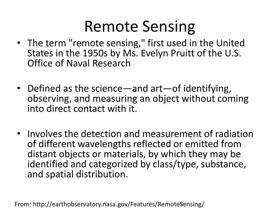
Remote Sensing Process Example
1. Energy Source or Illumination (A)
2. Radiation and the Atmosphere (B)
3. Interaction with the Target (C)
From: http://www.nrcan.gc.ca/earth-sciences/geography-boundary/remote-sensing/fundamentals/1924/
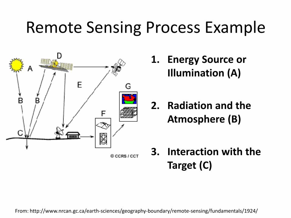
Remote Sensing Process Example
4. Recording of Energy by the Sensor (D)
5. Transmission, Reception, and Processing (E)
6. Interpretation and Analysis (F)
7. Application (G) From: http://www.nrcan.gc.ca/earth-sciences/geography-boundary/remote-sensing/fundamentals/1924/

Electromagnetic Spectrum
• Electromagnetic radiation is emitted at different wavelengths and frequencies
• Remote sensing generally involves use of the ultraviolet to microwave portions of the spectrum
From: http://www.nrcan.gc.ca/earth-sciences/geography-boundary/remote-sensing/fundamentals/1924/

Spectral Signatures
• For any given material, the amount of solar radiation that reflects, absorbs, or transmits varies with wavelength.
• This important property of matter makes it possible to identify different substances or classes and separate them by their spectral signatures (spectral curves)
From: http://www.fas.org/irp/imint/docs/rst/Intro/Part2_5.html

Spectral Signatures for Identifying Water Ponds
)2(
)3(
bRED
bNIRBandRatio
Band Ratio < 1.0 is identified as “clear water”
Cloud
Cloud Shadow
Vegetation Indices
• Uses differential between red and near infrared reflectance as measured by the satellite
• Actively growing plants show a contrast between strong absorption in the red and high reflectance in the near-infrared regions of the spectrum.
• The amount of absorption in the red and reflectance in the near-infrared varies with both the type of vegetation and the vigor of the plants.
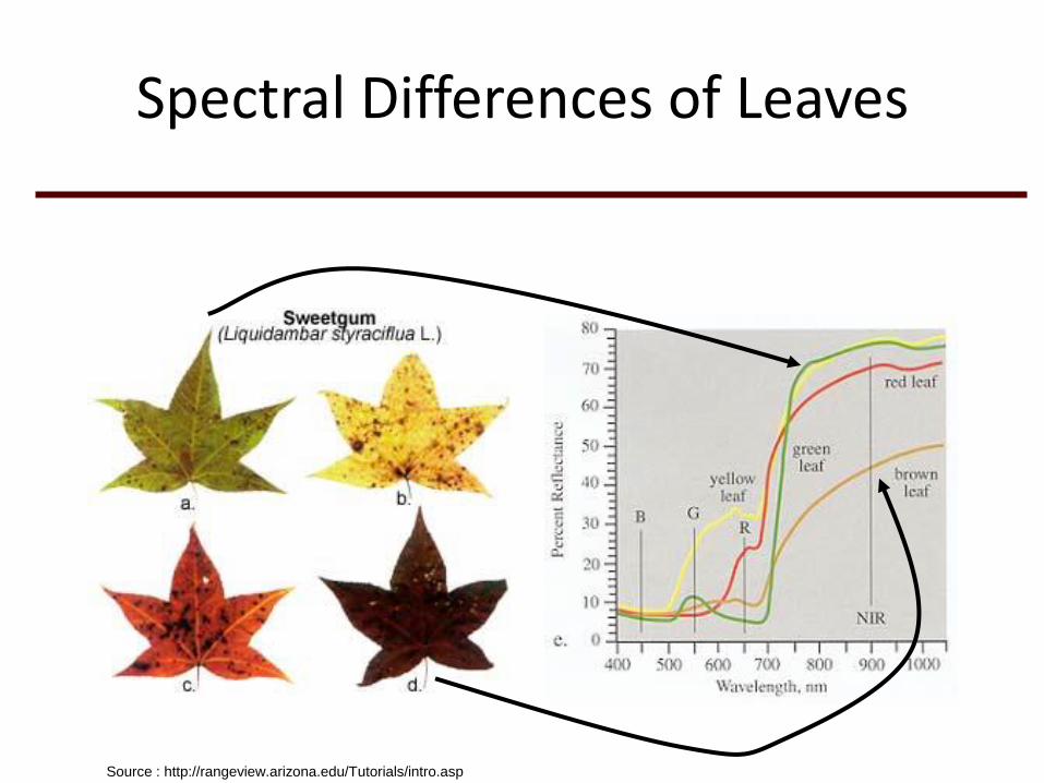
Spectral Differences of Leaves
Source : http://rangeview.arizona.edu/Tutorials/intro.asp

NDVI Calculation
Calculated as NDVI = (NIR - VIS)/(NIR + VIS)
Source : http://earthobservatory.nasa.gov/Library/MeasuringVegetation/measuring_vegetation_2.html

!
!
!!
!
!
!
Altai
Sainshand
Mandalgobi
Arvaikheer
Dalanzadgad
Bayankhongor
NDVI – Vegetation Greenness
• Normalized Difference Vegetation Index (NDVI) is a satellite derived measurement of vegetation greenness
• NDVI is generally correlated to vegetation biomass in most regions
• Useful for many different applications
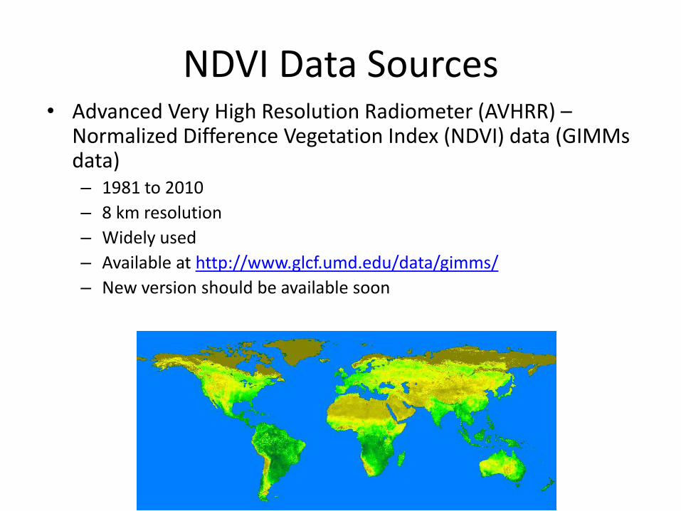
NDVI Data Sources • Advanced Very High Resolution Radiometer (AVHRR) –
Normalized Difference Vegetation Index (NDVI) data (GIMMs data) – 1981 to 2010
– 8 km resolution
– Widely used
– Available at http://www.glcf.umd.edu/data/gimms/
– New version should be available soon

Data Sources • Moderate Resolution Imaging Spectroradiometer (MODIS)
NDVI and Enhanced Vegetation Index (EVI) – 1 km, 500m, and 250 m resolution
– Available from 2000 to present
– Enhanced Vegetation Index (EVI) product builds in algorithms to adjust for soil distortions and canopy saturation
– Available from https://lpdaac.usgs.gov/get_data/data_pool
– Requires resampling and processing for use in GIS

Data Sources
• Expedited MODIS (eMODIS) – New product available from USGS
– 2000 to present
– Expedited means data are available within one day of last image acquisition in the composite window
– Resolution of 250m
– Geographic Projection
– Available for Asia region
– Download from:
– http://dds.cr.usgs.gov/emodis/CentralAsia/
Vegetation Condition Index
• Vegetation Condition Index is calculated by scaling NDVI for period of interest to the historical minimum and maximum
– (Current NDVI – minNDVI) / (maxNDVI – minNDVI) * 100
– Values less than 30 are considered drought
– Examine spatial extent and occurrence/intensity of drought for the time series
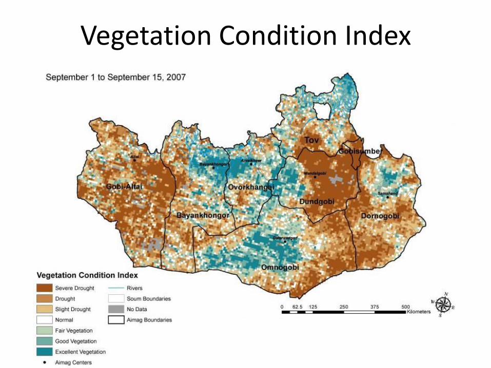
Vegetation Condition Index

Historical Time Series Analysis
• Time series analysis to examine trends in satellite greenness (NDVI) for historical record (nationwide) –Patterns of green-up and senescence
–Patterns in integrated NDVI (proxy for
biomass accumulation)
– Trends in vegetation condition index

Time Series Analysis
• TIMESAT software will be used for the developing the time series data – Calculates yearly beginning of season, end of season, amplitude,
integrated NDVI values
– Available from: http://www.nateko.lu.se/TIMESAT/timesat.asp?cat=0
Green-up End of Season
Integrated NDVI

Time Series Variables
a. Start of Season - time of year for the start of vegetation green-up
b. End of Season - time for which the vegetation greenness and biomass accumulation is declining

Time Series Variables
f. Seasonal amplitude - difference between the maximum greenness value and the base level.
g. Length of the season - time from
the start to the end of the season.
h. Small Seasonal Integral - integral of the difference between the function describing the season and the base level from season start to season end.
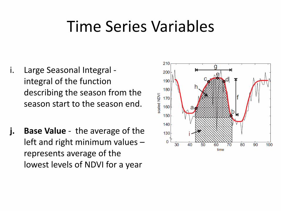
Time Series Variables
i. Large Seasonal Integral - integral of the function describing the season from the season start to the season end.
j. Base Value - the average of the left and right minimum values – represents average of the lowest levels of NDVI for a year

Mapping Time Series Output Start of Season

Mapping Time Series Output End of Season

Mapping Time Series Output Season Large Integral
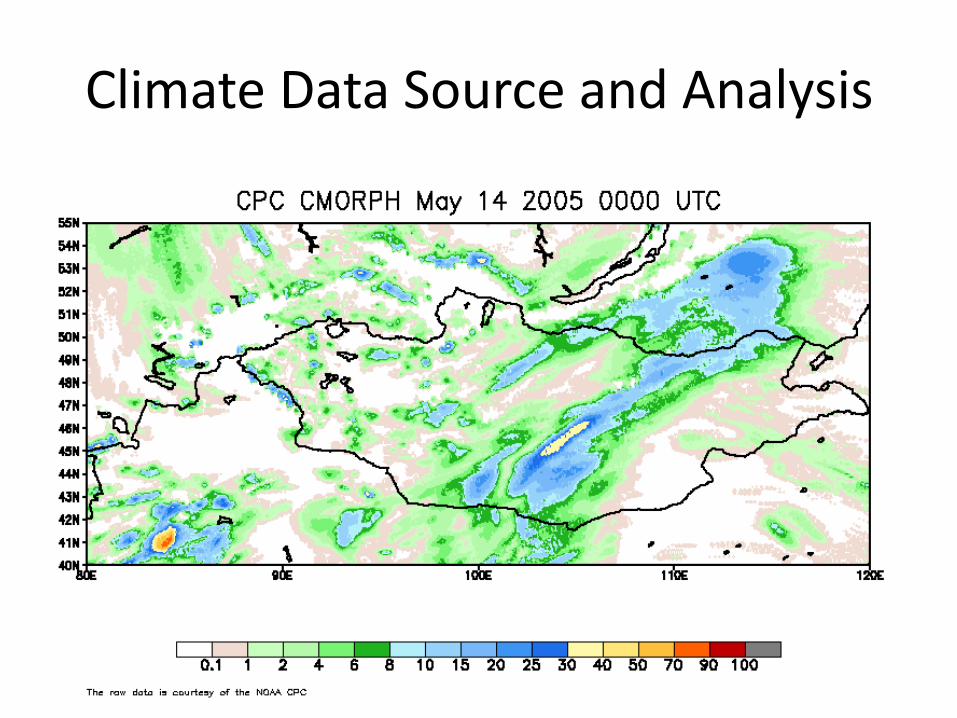
Climate Data Source and Analysis

Data Sources • Unified Precipitation Dataset
– Product available from NOAA that uses optimal interpolation
– 0.50 degree resolution (~55 km) – Daily Product, 1979 to present – Available from:
ftp://ftp.cpc.ncep.noaa.gov/precip/CPC_UNI_PRCP/GAUGE_GLB/
• Global Telecommunications System (GTS) Station Data
– Daily climate data for reporting World Meteorological Organization (WMO) stations
– Includes about 26 stations in Mongolia – Archived by Texas A&M (2003 to present) – Station History (ftp://ftp.ncdc.noaa.gov/pub/data/gsod/ish-
history.txt)

APHRODITE: Asian Precipitation - Highly-Resolved
Observational Data Integration Towards Evaluation of Water Resources
• Daily, gridded rainfall and temperature data set for Asia – Resolution: 0.25° and 0.50°
– Interpolated surfaces from a variety of climate data sources
– Time period is 1951-2007
– Monsoon Asia product
– Data Available at:
http://www.chikyu.ac.jp/precip/index.html

APHRODITE Coverage
From: http://www.chikyu.ac.jp/precip/index.html

APHRODITE Data Sources • Individual collection - Negotiation with local
meteorological/hydrological organizations and/or local researchers
• Pre-compiled datasets Global Historical Climatology Network (GHCN) Carbon Dioxide Information Analysis Center (CDIAC) National Center for Atmospheric Research, Data Archive (NCAR-DS) National Climatic Data Center (NCDC) Food and Agriculture Organization of the United Nations (FAO) GEWEX Asian Monsoon Experiment-Tropics (GAME-T) data center The Mekong River Commission (MRC) European Climate Assessment & Dataset (ECAD)
• Global Telecommunication System

World Clim Data
• Monthly interpolated surfaces of climate data
• Resolution – 1 km
• Several Variables Available:
– Min. Temperature
– Max. Temperature
– Mean Temperature
– Precipitation
– Derived Bioclimatic Variables

World Clim Data
• Monthly interpolated surfaces of climate data
• Resolution – 1 km
• Several Variables Available:
– Min. Temperature
– Max. Temperature
– Mean Temperature
– Precipitation
– Derived Bioclimatic Variables

World Clim Data
• Data Sources – – Global Historical Climatology Network (GHCN), – FAO – WMO – International Center for Tropical Agriculture (CIAT), R-Hydronet – Climate databases for Australia, New Zealand, the Nordic European
Countries, Ecuador, Peru, Bolivia, among others.
• Interpolated using the the ANUSPLIN software using latitude, longitude, and elevation as independent variables
• Time period is 1950 to 2000
• Data available online at: http://www.worldclim.org/download

Rainfall Coefficient of Variability (CV) Mapping
• The CV of annual rainfall has been suggested as a threshold indicator for equilibrium vs. non-equilibrium conditions on rangelands
• Areas having CVs of greater than 33% may be indicative of non-equilibrium conditions
• Interpolated rainfall time series provide a means to examine the spatial extent of areas having high rainfall variability
• The data can be analyze to map the CV to identify potential equilibrium/non-equilibrium zones

Rainfall CV Mapping
von Wehrden, H., J. Hanspach, P. Kaczensky, J. Fischer and K. Wesche. 2012. A global assessment of the non-equilibrium concept in rangelands. Ecological Applications, 22(2):393-399
Texas A&M splining of WMO Dataset
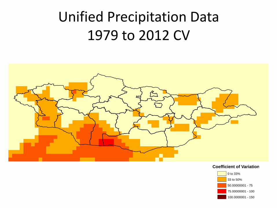
Unified Precipitation Data 1979 to 2012 CV
Coefficient of Variation
0 to 33%
33 to 50%
50.00000001 - 75
75.00000001 - 100
100.0000001 - 150
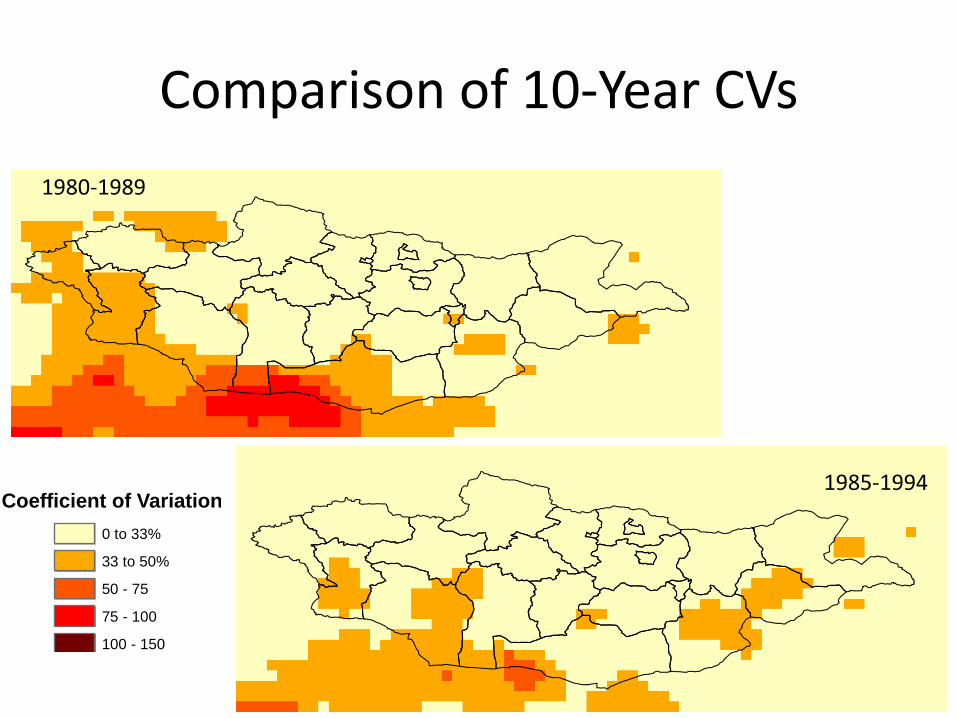
Comparison of 10-Year CVs
1980-1989
1985-1994 Coefficient of Variation
0 to 33%
33 to 50%
50 - 75
75 - 100
100 - 150

Comparison of 10-Year CVs
1990-1999
1995-2004
Coefficient of Variation
0 to 33%
33 to 50%
50 - 75
75 - 100
100 - 150

Comparison of 10-Year CVs 2000-2009
2003-2012
Coefficient of Variation
0 to 33%
33 to 50%
50 - 75
75 - 100
100 - 150

Next Steps
• Examine other climate data sets (WorldClim and APHRODITE) to see if similar patterns emerge.
• Compare interpolation methods
Integration with GIS and other Remote Sensing Data
• GIS provides a means of examining information in relation to boundaries, locations, and other remote sensing data
• Integration of imagery with other Remote sensing products like digital elevation models (DEM) can allow examination of data by slope, aspect, etc.

Data Data can be created in-house, downloaded, or
purchased.
Two types:
Spatial data: map, photos, graphics
Attribute data: descriptions, database
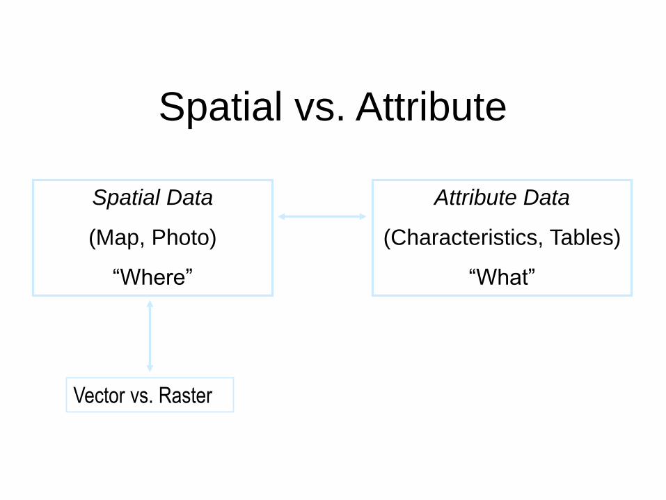
Spatial vs. Attribute
Spatial Data
(Map, Photo)
“Where”
Attribute Data
(Characteristics, Tables)
“What”
Vector vs. Raster

Spatial Data
Represented by:
Points
Lines
Polygons
Geographic representation of data
vector

Spatial Attribute
id_no name length (f)
1 Deer Trail 500
2 Spring Lane 750
3 Woods Road 1000
id_no acres infestation spread_rate
1 4 SPB 4/m
2 3.5 SPB 12/m
points
lines
polygons
points, lines, polygons
id_no nest_type eggs condition
1 rcw 4 good
2 cardinal 0 fair
3 bluebird 3 fair
4 rcw 2 good
5 cardinal 6 good

GIS

Vector Data
• Points, Lines, Polygons
• Can be used to describe real world features such as roads, property boundaries, pipelines, cities, deer blinds, transect locations, etc.
• Attributes can give details about a feature such as name, length, transect production, deer counts etc.

Example of Vector Data

Attribute Data

Raster Data
• Comprised of Pixels
• Pixel size determines resolution
• Examples:
– Satellite imagery
– Aerial Imagery
– Radar
– LIDAR
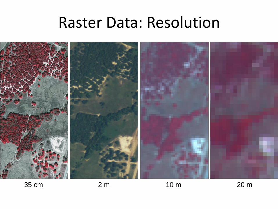
Raster Data: Resolution
35 cm 2 m 10 m 20 m

Normalized Difference Vegetation Index (NDVI) Product – 250 m resolution
Integrating Data with Boundary and Other Useful Information

Enhanced Vegetation Index (EVI) Product – 250 m resolution
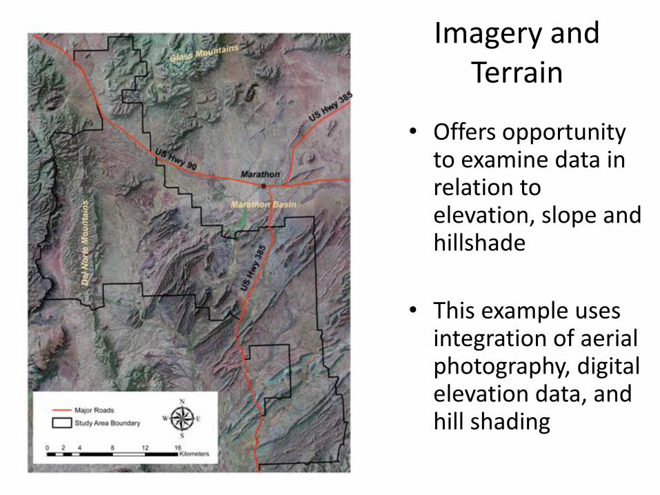
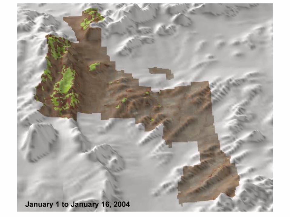
Imagery and Terrain
• Offers opportunity
to examine data in relation to elevation, slope and hillshade
• This example uses integration of aerial photography, digital elevation data, and hill shading

Integrating With a GIS

Integrating With a GIS !
!
!
!
!
!
!
!O8a
O4a
O2a
O6a
O7a
O5a
O1a

Other Products Useful For Rangelands
• Google Earth • NASA, USGS, and NOAA's Landsat satellite program
with the following sensors: – Multispectral Scanner (MSS) – Thematic Mapper (TM) and Enhanced Thematic Mapper
(ETM+) – http://landsat.usgs.gov/products_data_at_no_charge.php
• Ikonos • Quickbird • Digital Elevation Data
– Shuttle Radar Topography Mission (http://srtm.usgs.gov/index.php)
– ASTER Global Digital Elevation Map (http://asterweb.jpl.nasa.gov/gdem.asp)

Questions or Comments?