Remarks; Model sessions JJ II - UC3Mhalweb.uc3m.es/esp/Personal/personas/bdauria/1112/Sidney... ·...

Remarks

Intro

Sessions

Distn Structure

Dependence

Finale

Title Page

JJ II

J I

of 42

Go Back

Full Screen

Close

Quit

Remarks; Model sessionsusing peak rate covariate

Sidney ResnickSchool of Operations Research and Information Engineering

Rhodes Hall, Cornell UniversityIthaca NY 14853 USA

http://legacy.orie.cornell.edu/∼[email protected]

Madrid

May 24, 2012

Work with: Luis Lopez-Oliveros

Remarks

Intro

Sessions

Distn Structure

Dependence

Finale

Title Page

JJ II

J I

of 42

Go Back

Full Screen

Close

Quit

1. Remarks and amplification.

1.1. How to construct distribution with regularly varying tail on[0,∞] \ {0} with specified angular measure.

Easiest method: Given a distribution S on the unit sphere, let Θ be arandom vector with distribution S and let R be Pareto(1) and define

X = RΘ.

Remarks

Intro

Sessions

Distn Structure

Dependence

Finale

Title Page

JJ II

J I

of 42

Go Back

Full Screen

Close

Quit

Remarks

Intro

Sessions

Distn Structure

Dependence

Finale

Title Page

JJ II

J I

of 42

Go Back

Full Screen

Close

Quit

1.2. Example: Same rv’s; different variation on different cones.

Let X and Z be iid Pareto(1) random variables and define

Y = X2 ∧ Z2.

Then in E,E0 and Eu check convergence on representative relativelycompact sets:

• In M+(E), asymptotic independence,

tP[(

X

t,Y

t

)∈ ([0, x]× [0, y])c

]→ 1

x+

1

y, x ∨ y > 0.

• In M+(E0):

tP[(

X

t2/3,Y

t2/3

)∈ (x,∞]× (y,∞]

]→ 1

x√y, x ∧ y > 0,

or in standard form,

tP[(

X3/2

t,Y 3/2

t

)∈ (x,∞]× (y,∞]

]→ 1

x2/3y1/3, x ∧ y > 0.

Remarks

Intro

Sessions

Distn Structure

Dependence

Finale

Title Page

JJ II

J I

of 42

Go Back

Full Screen

Close

Quit

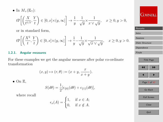
• In M+(Eu):

tP[(

X

t1/2,Y

t

)∈ [0, x]×(y,∞]

]→ 1

y− 1√y× 1

x ∨√y, x ≥ 0, y > 0,

or in standard form,

tP[(

X2

t,Y

t

)∈ [0, x]×(y,∞]

]→ 1

y− 1√y× 1√

x ∨√y, x ≥ 0, y > 0.

1.2.1. Angular measures

For these examples we get the angular measure after polar co-ordinatetransformation

(x, y) 7→ (r, θ) := (x+ y,x

x+ y).

• On E,

S(dθ) =1

2[ε{0}(dθ) + ε{1}(dθ)],

where recall

εx(A) =

{1, if x ∈ A;

0, if x /∈ A.

Remarks

Intro

Sessions

Distn Structure

Dependence

Finale

Title Page

JJ II

J I

of 42

Go Back

Full Screen

Close

Quit

• For the standard form on E0 we have the angular measure

S(dθ) =1

θ5/3(1− θ)4/3dθ, 0 < θ < 1.

The density is not integrable near 0 or 1 so S is not a finite measureon (0, 1). Could change to a compact region in a neighborhood of∞.

• For the standard form on Eu

S(dθ) =

{θ−

32 (1− θ)− 3

2dθ, 12≤ θ < 1

0 0 ≤ θ < 12.

This is not integrable near 1 so S is not finite on [0, 1).

1.2.2. Angular measure finite or infinite?

Example of class of examples of standard regular variation on Eu in-dexed by distributions on [0,∞]. Suppose

R ∼ Pareto(1) on [1,∞), θ ≥ 0, θ ∼ G(·) on [0,∞].

Assume R ⊥⊥ θ. Define

(X, Y ) = (Rθ,R).

Remarks

Intro

Sessions

Distn Structure

Dependence

Finale

Title Page

JJ II

J I

of 42

Go Back

Full Screen

Close

Quit

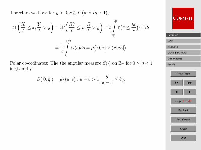
Therefore we have for y > 0, x ≥ 0 (and ty > 1),

tP(X

t≤ x,

Y

t> y

)= tP

(Rθ

t≤ x,

R

t> y

)= t

∞∫ty

P(θ ≤ tx

r

)r−2dr

=1

x

x/y∫0

G(s)ds = µ([0, x]× (y,∞]

).

Polar co-ordinates: The the angular measure S(·) on Eu for 0 ≤ η < 1is given by

S([0, η]) = µ{(u, v) : u+ v > 1,y

u+ v≤ θ}.

Remarks

Intro

Sessions

Distn Structure

Dependence

Finale

Title Page

JJ II

J I

of 42

Go Back

Full Screen

Close

Quit

Hence

tP

[X + Y

t> 1,

X

X + Y≤ η

]= tP

[Rθ +R

t> 1,

Rθ

Rθ +R≤ η

]= tP

[R(1 + θ)

t> 1, θ ≤ η

1− η

]= t

∫0≤s≤ η

1−η

P

[R

t(1 + s) > 1

]G(ds)

→∫0≤s≤ η

1−η

(1 + s)G(ds) =: S[0, η].

Hence

S([0, η]) =

∫0≤s≤ η

1−η

(1 + s)G(ds), 0 ≤ η < 1.

Conclude: S is a finite angular measure on [0, 1) if and only if G hasfirst moment.

Remarks

Intro

Sessions

Distn Structure

Dependence

Finale

Title Page

JJ II

J I

of 42

Go Back

Full Screen

Close

Quit

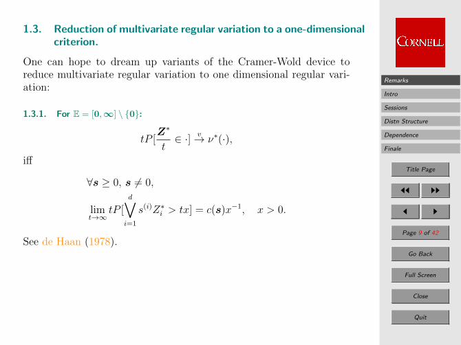
1.3. Reduction of multivariate regular variation to a one-dimensionalcriterion.

One can hope to dream up variants of the Cramer-Wold device toreduce multivariate regular variation to one dimensional regular vari-ation:

1.3.1. For E = [0,∞] \ {0}:

tP [Z∗

t∈ ·] v→ ν∗(·),

iff

∀s ≥ 0, s 6= 0,

limt→∞

tP [d∨i=1

s(i)Z∗i > tx] = c(s)x−1, x > 0.

See de Haan (1978).

Remarks

Intro

Sessions

Distn Structure

Dependence

Finale

Title Page

JJ II

J I

of 42

Go Back

Full Screen

Close

Quit

1.3.2. For E0 = (0,∞] and HRV:

Hidden regular variation requires checking regular variation on E0. Forevery a ≥ 0,a 6= 0,

∧di=1 a

(i)Z(i) has a regularly varying distributiontail of index α0.

Remarks

Intro

Sessions

Distn Structure

Dependence

Finale

Title Page

JJ II

J I

of 42

Go Back

Full Screen

Close

Quit

1.4. Two examples of how to construct distribution with HRV.

Example 1: d = 2; independent random quantities B,Y ,U with

P [B = 0] = P [B = 1] = 1/2

and Y = (Y (1), Y (1)) is iid with

P [Y (1) > x] = x−1, x > 1

andb(t) = t.

Let U have multivariate regularly varying distribution on E and∃α0 > 1, b0(t) ∈ RV1/α0 , ν0 6≡ 0,

tP [U

b0(t)∈ ·]→ ν0 6= 0.

DefineZ = BY + (1−B)U

which has hidden regular variation, and the property

S0(ℵ0) := ν0{x ∈ E0 : ‖x‖ > 1} <∞.

Remarks

Intro

Sessions

Distn Structure

Dependence

Finale

Title Page

JJ II

J I

of 42

Go Back

Full Screen

Close

Quit

Example 2: For d = 2, define Z = (Z(1), Z(2)) iid and Paretodistributed with

P [Z(1) > x] = x−1, x > 1, i = 1, 2.

Setb(t) = t, b0(t) =

√t,

so that b(t)/b0(t) → ∞. Then Z is asymptotically independentand possesses hidden regular variation with

ν0([x,∞]

)=(x1x2

)−1.

On EtP [

Z

b(t)∈ ·] v→ ν,

ν(E0) = 0, and on E0

tP [Z

b0(t)∈ ·] v→ ν0,

andS0(ℵ0) := ν0{x ∈ E0 : ‖x‖ > 1} =∞.

Remarks

Intro

Sessions

Distn Structure

Dependence

Finale

Title Page

JJ II

J I

of 42

Go Back

Full Screen

Close

Quit

HRV follows from

tP [Z(1) >√tx, Z(2) >

√ty]

=√tP [P [Z(1) >

√tx]√tP [P [Z(2) >

√ty]

→ 1

xy.

Remarks

Intro

Sessions

Distn Structure

Dependence

Finale

Title Page

JJ II

J I

of 42

Go Back

Full Screen

Close

Quit

2. Network Input Models Based on Peak Rate in Sessions–where asymptotic independence does not rule.

Session: higher order construct typically obtained by amalgamatingeither

• packets (see Part II)

• connections

• groups of connections.

according to some chosen – and not unique– definition.

Recall modeling Approach

Sessions characterized by

• Initiation times {Γk} where often assume for tractability

{Γk} ∼ Poisson, rate λ.

• The mark or session descriptor of Γk:

(Sk, Dk, Rk) = (Size, Duration, Rate ),

where R is average rate in session:

Rk = Sk/Dk.

Remarks

Intro

Sessions

Distn Structure

Dependence

Finale

Title Page

JJ II

J I

of 42

Go Back

Full Screen

Close

Quit

Assessing dependence structure of (S,D,R).

Consider

S = file size, total info in session, # bytes

D = duration of transmission or session,

R = throughput, rate = F/L.

All three, are usually (alas–not always) empirically seen to be heavytailed:

P [S > x] =x−αS`S(x)

P [L > x] =x−αD`D(x)

P [R > x] =x−αR`R(x).

Note: Segmenting data in various ways (eg by peak rate) may precludecertain segments from having R heavy tailed.

Remarks

Intro

Sessions

Distn Structure

Dependence

Finale

Title Page

JJ II

J I

of 42

Go Back

Full Screen

Close

Quit

Empirical–Statistical Modeling from Packet Headers

Plausible goals:

• How to model Internet transmissions based on collected data ofindividual packet headers?

• Since the Internet behaves partly as a result of human stimulation,hope somewhere in this mess of data there lurk Poisson points.

• How to amalgamate packets into higher order entities which sim-plifiy modeling and allow fluid or continuous type models?

• What entity arrival times can plausibly be regarded as derivedfrom Poisson?

• Teach a computer to mimic Internet sessions and hence end userInternet behavior.

Remarks

Intro

Sessions

Distn Structure

Dependence

Finale

Title Page

JJ II

J I

of 42

Go Back

Full Screen

Close

Quit

3. Data sessions

Definition 1 (Sarvotham et al. (2005)) A session is a cluster ofpackets with same source and destination network addresses, such thatthe delay between any two succesive packets in the cluster is less thana threshold t(= 2s).

Other definitions possible.

3.1. Session descriptors:

For each session, compute the following descriptors:

• S : Number of bytes transmitted (size).

• D : Duration of the session.

• R = S/D : Average transfer rate.

• Γ: Starting time.

• For studying burstiness, some measure of peak rate.

Remarks

Intro

Sessions

Distn Structure

Dependence

Finale

Title Page

JJ II

J I

of 42

Go Back

Full Screen

Close

Quit

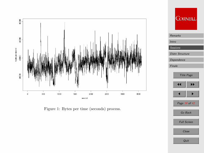
3.2. Sample data set.

http://wand.cs.waikato.ac.nz/wits/

• TCP traffic (www, email, FTP)

• Traffic sent to a University of Auckland server on December 8,1999, between 3 and 4 pm.

• Raw data: 1,177,497 packet headers.

• Harvest working data set of the form {(Si, Di, Ri,Γi) : 1 ≤ i ≤44, 136}.

Originally used by Sarvotham et al. (2005) to study of sources ofburstiness: Burstiness is important in order to understand congestionbecause of the sudden peak loads it introduces to the network; qosconcerns.

http://wand.cs.waikato.ac.nz/wits/

Remarks

Intro

Sessions

Distn Structure

Dependence

Finale

Title Page

JJ II

J I

of 42

Go Back

Full Screen

Close

Quit

Figure 1: Bytes per time (seconds) process.

Remarks

Intro

Sessions

Distn Structure

Dependence

Finale

Title Page

JJ II

J I

of 42

Go Back

Full Screen

Close

Quit

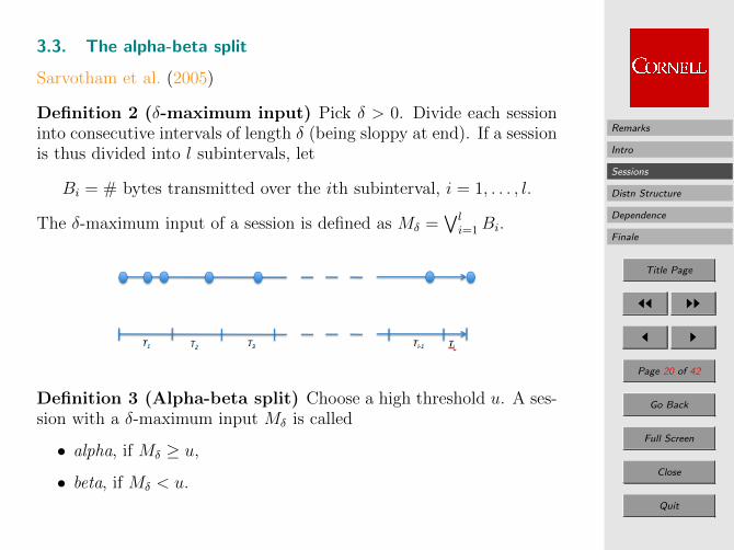
3.3. The alpha-beta split

Sarvotham et al. (2005)

Definition 2 (δ-maximum input) Pick δ > 0. Divide each sessioninto consecutive intervals of length δ (being sloppy at end). If a sessionis thus divided into l subintervals, let

Bi = # bytes transmitted over the ith subinterval, i = 1, . . . , l.

The δ-maximum input of a session is defined as Mδ =∨li=1Bi.

Definition 3 (Alpha-beta split) Choose a high threshold u. A ses-sion with a δ-maximum input Mδ is called

• alpha, if Mδ ≥ u,

• beta, if Mδ < u.

Remarks

Intro

Sessions

Distn Structure

Dependence

Finale

Title Page

JJ II

J I

of 42

Go Back

Full Screen

Close

Quit

Empirical features

Sarvotham et al. (2005) found:

• Alpha-sessions are the major source of burstiness.

• In alpha-sessions: R ⊥⊥ S (sort of).

• In beta-sessions: R ⊥⊥ D (sort of).

• Split usually produces huge beta-group (≈ tens of thousands) vs.tiny alpha-group (< 100).

• Implies segmented sessions have different distribution in each seg-ment.

Does further segmentation of the beta-group produce meaningful in-formation?

Goals:

• Better description of dependence structure of (S,D,R) within seg-ment

• Simulation model.

Remarks

Intro

Sessions

Distn Structure

Dependence

Finale

Title Page

JJ II

J I

of 42

Go Back

Full Screen

Close

Quit

3.4. Finer segmentation

Split the data into m groups of approximately equal size according tothe empirical quantiles of the burstiness predictor or covariate; we hadto define a new definition of peak rate.

Will use m = 10 and speak of the decile groups. Split into decilegroups.

Features:

• Rather than a beta-group, we have 9 groups each with the peakrate covariate in a given decile range.

• Claim the alpha-beta split masks further structure and it is infor-mative to take into account the explicit level of the covariate.

Remarks

Intro

Sessions

Distn Structure

Dependence

Finale

Title Page

JJ II

J I

of 42

Go Back

Full Screen

Close

Quit

3.5. Peak rate

Definition 4 For a session with n packets:

B′i =# bytes in ith packet,

T ′i =interarrival time between ith and (i+ 1)st packet,

i = 1, . . . , n− 1. For k = 2, . . . , n, the peak rate of order k is

P (k) =n−k+1∨i=1

∑i+k−1j=i B′j∑i+k−2j=i T ′j

.

The P (k) is the maximum transfer rate using only k consecutive pack-ets.The peak rate is defined as

P∨ =n∨k=2

P (k).

[Makes sense empirically but would be difficult to work with analyti-cally.]

Remarks

Intro

Sessions

Distn Structure

Dependence

Finale

Title Page

JJ II

J I

of 42

Go Back

Full Screen

Close

Quit

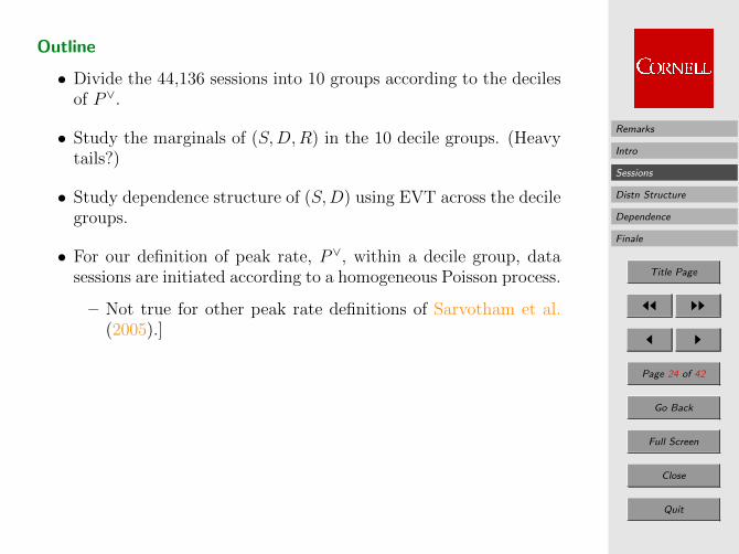
Outline

• Divide the 44,136 sessions into 10 groups according to the decilesof P∨.

• Study the marginals of (S,D,R) in the 10 decile groups. (Heavytails?)

• Study dependence structure of (S,D) using EVT across the decilegroups.

• For our definition of peak rate, P∨, within a decile group, datasessions are initiated according to a homogeneous Poisson process.

– Not true for other peak rate definitions of Sarvotham et al.(2005).]

Remarks

Intro

Sessions

Distn Structure

Dependence

Finale

Title Page

JJ II

J I

of 42

Go Back

Full Screen

Close

Quit

4. Structure of (S,D,R).

4.1. Heavy tails

Definition 5 Convenient to use the γ parameterization. Call Y hasheavy tailed if its cdf F satisfies

F (y) = y−1/γ`(y),

where ` is slowly varying and γ > 0.

Quickie summary:

• In each decile group, (S,D) jointly heavy tailed w/o asymptoticindependence.

• R is only heavy tailed for the highest decile group;

• R does not appear to be even in a domain of attraction for anyof the 9 lower decile groups.

Remarks

Intro

Sessions

Distn Structure

Dependence

Finale

Title Page

JJ II

J I

of 42

Go Back

Full Screen

Close

Quit

4.2. Estimation of γ’s

Definition 6 (Hill estimator) Let {X1, . . . , Xn} be iid (or station-ary + mixing) with order statistics

X1:n ≤ · · · ≤ Xn:n.

The Hill estimator of γ > 0 is

γk,n =1

k

n∑i=n−k+1

logXi:n

Xn−k:n. (1)

Theorem 1 (Consistency of Hill) If the distribution is heavy tailed+additional second order condition, as k →∞, n→∞, k/n→ 0:

√k(γk,n − γ)

d−→ N(0, γ2). (2)

Equivalent to peaks over threshold method and MLE.

Remarks

Intro

Sessions

Distn Structure

Dependence

Finale

Title Page

JJ II

J I

of 42

Go Back

Full Screen

Close

Quit

Figure 2: Size, duration and rate in the 10th decile group

Remarks

Intro

Sessions

Distn Structure

Dependence

Finale

Title Page

JJ II

J I

of 42

Go Back

Full Screen

Close

Quit

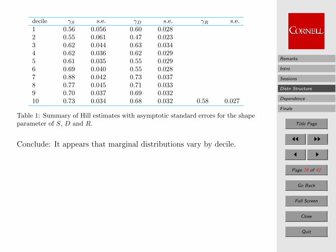
decile γS s.e. γD s.e. γR s.e.1 0.56 0.056 0.60 0.0282 0.55 0.061 0.47 0.0233 0.62 0.044 0.63 0.0344 0.62 0.036 0.62 0.0295 0.61 0.035 0.55 0.0296 0.69 0.040 0.55 0.0287 0.88 0.042 0.73 0.0378 0.77 0.045 0.71 0.0339 0.70 0.037 0.69 0.03210 0.73 0.034 0.68 0.032 0.58 0.027

Table 1: Summary of Hill estimates with asymptotic standard errors for the shapeparameter of S, D and R.

Conclude: It appears that marginal distributions vary by decile.

Remarks

Intro

Sessions

Distn Structure

Dependence

Finale

Title Page

JJ II

J I

of 42

Go Back

Full Screen

Close

Quit

5. Dependence structure of (S,D)

• Dependence structure varies by decile. Seen already in simplescatter plots.

• Assess dependence by computing angular measures which givefavored directions for big values of (S,D).

– Standardize the pairs to have the same tails by ranks method .

– Threshold the resulting pairs and keep only those data pairsoutside a large circle.

– Convert to polar coordinates.

– Make density plot of θ-coordinate.

Remarks

Intro

Sessions

Distn Structure

Dependence

Finale

Title Page

JJ II

J I

of 42

Go Back

Full Screen

Close

Quit

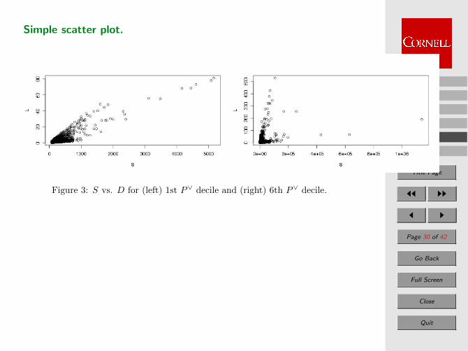
Simple scatter plot.

Figure 3: S vs. D for (left) 1st P∨ decile and (right) 6th P∨ decile.

Remarks

Intro

Sessions

Distn Structure

Dependence

Finale

Title Page

JJ II

J I

of 42

Go Back

Full Screen

Close

Quit

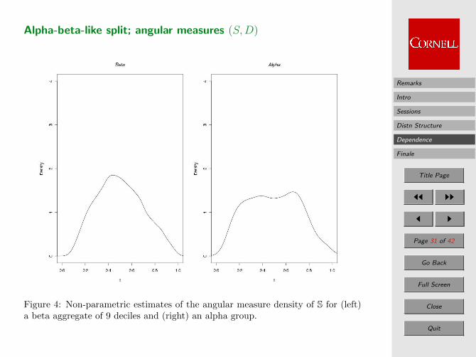
Alpha-beta-like split; angular measures (S,D)

Figure 4: Non-parametric estimates of the angular measure density of S for (left)a beta aggregate of 9 deciles and (right) an alpha group.

Remarks

Intro

Sessions

Distn Structure

Dependence

Finale

Title Page

JJ II

J I

of 42

Go Back

Full Screen

Close

Quit

Finer split: plots reasonably symmetric, unimodal

Figure 5: Non-parametric estimates of the angular measure density of S from leftto right and top to bottom: 1st to 9th decile groups.

Remarks

Intro

Sessions

Distn Structure

Dependence

Finale

Title Page

JJ II

J I

of 42

Go Back

Full Screen

Close

Quit

Comments

• Seek to relate the explicit level of P∨ with the dependence struc-ture of (S,D).

Seek global model: Hope the angular measure S can be approxi-mated by some Sψ where a (generalized linear) model links g(ψ) ∼decilegroup.

• Using QQ plots and sample acf’s can check within decile groups,session initiation times look Poisson. This is not true across thewhole data set–only when the data is segmented by decile group;also not true with other definitions of peak rate.

Remarks

Intro

Sessions

Distn Structure

Dependence

Finale

Title Page

JJ II

J I

of 42

Go Back

Full Screen

Close

Quit

5.1. Global model: Toward a parametric model for the angularmeasure density S

Logistic model:

hψ(t) =1

2

(1

ψ− 1

)t−1−1/ψ(1− t)−1−1/ψ[t−1/ψ + (1− t)−1/ψ]ψ−2, (3)

=h(t), 0 ≤ t ≤ 1,

with ψ ∈ (0, 1).

Features:

• Symmetric.

• For ψ < 0.5 : h is unimodal and as ψ → 0 we obtain perfectdependence.

• For ψ > 0.5 : h is bimodal and as ψ → 1 we obtain asymptoticindependence.

This allows us to quantify the effect of P∨ on the dependence betweenS and D.

Remarks

Intro

Sessions

Distn Structure

Dependence

Finale

Title Page

JJ II

J I

of 42

Go Back

Full Screen

Close

Quit

Parametric vs non-parametric density estimates.

Figure 6: Parametric estimates of the angular measure density S superimposed tonon-parametric counterparts, from left to right and top to bottom: 1st to 9th decilegroups.

Remarks

Intro

Sessions

Distn Structure

Dependence

Finale

Title Page

JJ II

J I

of 42

Go Back

Full Screen

Close

Quit

Dependence of (S,D) as a function of P∨

Fit a global trend logistic model where

g−1(ψ) = β0 + β1 log(P∨).

After some experimenting choose link function g

g(x) =1/2

1 + e−x.

Remarks

Intro

Sessions

Distn Structure

Dependence

Finale

Title Page

JJ II

J I

of 42

Go Back

Full Screen

Close

Quit

Sketch of simulation of heterogeneous traffic:

1. In the existing data set, each session has an associated P∨. Formthe EDF. Get a bootstrap sample of P∨ from this EDF and divideinto m = 10 samples according to the quantiles.

2. For each group, simulate the starting times of the sessions viahomogeneous Poisson process.

3. For each P∨j , compute the corresponding value of ψj from theGLM and use it to simulate an angle Θj from the logistic distri-bution.

4. Simulate the radius component Nj; use Pareto for the heavy tail.

5. Transform to Cartesian coordinates and then invert using fittedmarginal distributions to get back to the original scale where(Sj, Dj) do not have same tails.Compute Rj = Sj/Dj.

Remarks

Intro

Sessions

Distn Structure

Dependence

Finale

Title Page

JJ II

J I

of 42

Go Back

Full Screen

Close

Quit

What about R?

• Except for highest decile, R is not in a domain of attraction andnot heavy tailed.

• We have evidence that

R− β(t)

α(t)

∣∣∣S > t⇒ G(·)

for α(t) > 0 and G a pm.

Allows application of an emerging theory of conditional extremevalues (CEV).

• Evidence that R|D cannot be modeled. How come?

Credit:

Lopez-Oliveros and Resnick (2009) + ideas of Jan Heffernan.

Remarks

Intro

Sessions

Distn Structure

Dependence

Finale

Title Page

JJ II

J I

of 42

Go Back

Full Screen

Close

Quit

6. Final thoughts

• Consistency issues for (S,D,R) where S/D = R. Why are

– (S,D) jointly heavy tailed and

– R|S > t has a limiting type

consistent.

Need theory to match empirical observation.

• Segmentation of sessions by application?

• Conditional on (deciles of) peak rate, sessions arrive according toa homogeneous Poisson. Use this theoretically. Overall traffic isa mixture?

• Sessions are better behaved after conditioning on peak rate. Butpeak rate is difficult to analyze based on packet level models.

Remarks

Intro

Sessions

Distn Structure

Dependence

Finale

Title Page

JJ II

J I

of 42

Go Back

Full Screen

Close

Quit

References

L. Breiman. On some limit theorems similar to the arc-sin law. TheoryProbab. Appl., 10:323–331, 1965.

L. de Haan. A characterization of multidimensional extreme-value dis-tributions. Sankhya Ser. A, 40(1):85–88, 1978. ISSN 0581-572X.

R. Gaigalas and I. Kaj. Convergence of scaled renewal processes and apacket arrival model. Bernoulli, 9(4):671–703, 2003. ISSN 1350-7265.

I. Kaj. Convergence of scaled renewal processes o fractional brownianmotion. Preprint: Department of Mathematics, Uppsala University,Box 480, S-751 06 Uppsala, Sweden, 1999.

I. Kaj. Stochastic Modeling in Broadband Communications Systems.SIAM Monographs on Mathematical Modeling and Computation.Society for Industrial and Applied Mathematics (SIAM), Philadel-phia, PA, 2002. ISBN 0-89871-519-9.

I. Kaj and M.S. Taqqu. Convergence to fractional brownian motion andto the telecom process: the integral representation approach. Avail-able at Department of Mathematics, Uppsala University, U.U.D. M.2004:16; To appear: Brazilian Probability School, 10th anniversaryvolume, Eds. M.E. Vares, V. Sidoravicius, Birkhauser 2007., 2004.

Remarks

Intro

Sessions

Distn Structure

Dependence

Finale

Title Page

JJ II

J I

of 42

Go Back

Full Screen

Close

Quit

T. Konstantopoulos and S.J. Lin. Macroscopic models for long-rangedependent network traffic. Queueing Systems Theory Appl., 28(1-3):215–243, 1998. ISSN 0257-0130.

L. Lopez-Oliveros and S.I. Resnick. Extremal dependence analysis ofnetwork sessions. Technical report, School of ORIE, Cornell Univer-sity, 2009. URL http://arxiv.org/pdf/0905.1983v1. to appear:Extremes .

T. Mikosch and A. Stegeman. The interplay between heavy tailsand rates in self-similar network traffic. Technical Report. Uni-versity of Groningen, Department of Mathematics, Available viawww.cs.rug.nl/eke/iwi/preprints/, 1999.

T. Mikosch, S.I. Resnick, H. Rootzen, and A.W. Stegeman. Is networktraffic approximated by stable Levy motion or fractional Brownianmotion? Ann. Appl. Probab., 12(1):23–68, 2002.

S.I. Resnick. Modeling data networks. In B. Finkenstadt andH. Rootzen, editors, SemStat: Seminaire Europeen de Statistique,Extreme Values in Finance, Telecommunications, and the Environ-ment, pages 287–372. Chapman-Hall, London, 2003.

S.I. Resnick and E. van den Berg. Weak convergence of high-speednetwork traffic models. J. Appl. Probab., 37(2):575–597, 2000.

http://arxiv.org/pdf/0905.1983v1

Remarks

Intro

Sessions

Distn Structure

Dependence

Finale

Title Page

JJ II

J I

of 42

Go Back

Full Screen

Close

Quit

S. Sarvotham, R. Riedi, and R. Baraniuk. Network and user driven on-off source model for network traffic. Computer Networks, 48:335–350,2005. Special Issue on Long-range Dependent Traffic.

Remarks; Model sessions JJ II - UC3Mhalweb.uc3m.es/esp/Personal/personas/bdauria/1112/Sidney... ·...

Documents

Transcript of Remarks; Model sessions JJ II - UC3Mhalweb.uc3m.es/esp/Personal/personas/bdauria/1112/Sidney... ·...