RelSen: An Optimization-based Framework for SimultaneouslySensor Reliability Monitoring and Data Cleaning

Cheng Feng, Xiao Liang, Daniel Schneegass, PengWei TianSiemens Corporate Technology

Beijing, China{cheng.feng,liang.xiao,daniel.schneegass,pengwei.tian}@siemens.com

ABSTRACTRecent advances in the Internet of Things (IoT) technology have ledto a surge on the popularity of sensing applications. As a result, peo-ple increasingly rely on information obtained from sensors to makedecisions in their daily life. Unfortunately, in most sensing applica-tions, sensors are known to be error-prone and their measurementscan become misleading at any unexpected time. Therefore, in or-der to enhance the reliability of sensing applications, apart fromthe physical phenomena/processes of interest, we believe it is alsohighly important to monitor the reliability of sensors and cleanthe sensor data before analysis on them being conducted. Existingstudies often regard sensor reliability monitoring and sensor datacleaning as separate problems. In this work, we propose RelSen, anovel optimization-based framework to address the two problemssimultaneously via utilizing the mutual dependence between them.Furthermore, RelSen is not application-specific as its implementa-tion assumes a minimal prior knowledge of the process dynamicsunder monitoring. This significantly improves its generality andapplicability in practice. In our experiments, we apply RelSen onan outdoor air pollution monitoring system and a condition moni-toring system for a cement rotary kiln. Experimental results showthat our framework can timely identify unreliable sensors and re-move sensor measurement errors caused by three types of mostcommonly observed sensor faults.

CCS CONCEPTS• Information systems → Sensor networks; Data cleaning; •General and reference → Reliability.

KEYWORDSsensor reliability monitoring, data cleaning, optimization

ACM Reference Format:Cheng Feng, Xiao Liang, Daniel Schneegass, PengWei Tian. 2020. RelSen:An Optimization-based Framework for Simultaneously Sensor ReliabilityMonitoring and Data Cleaning. In Proceedings of the 29th ACM InternationalConference on Information and Knowledge Management (CIKM ’20), October19–23, 2020, Virtual Event, Ireland. ACM, New York, NY, USA, 10 pages.https://doi.org/10.1145/3340531.3411942

Permission to make digital or hard copies of all or part of this work for personal orclassroom use is granted without fee provided that copies are not made or distributedfor profit or commercial advantage and that copies bear this notice and the full citationon the first page. Copyrights for components of this work owned by others than theauthor(s) must be honored. Abstracting with credit is permitted. To copy otherwise, orrepublish, to post on servers or to redistribute to lists, requires prior specific permissionand/or a fee. Request permissions from permissions@acm.org.CIKM ’20, October 19–23, 2020, Virtual Event, Ireland© 2020 Copyright held by the owner/author(s). Publication rights licensed to ACM.ACM ISBN 978-1-4503-6859-9/20/10. . . $15.00https://doi.org/10.1145/3340531.3411942

1 INTRODUCTIONWith the trend of IoT, sensors are becoming ubiquitous. The mea-surements from sensors have become an important source of knowl-edge to decision making for both human-beings and computingmachines in different domains, such as industrial process control[18], air pollution monitoring [10] and traffic flow measurement[16]. Nevertheless, it is also well known that measurements fromsensors (especially commodity sensors which are widely used inIoT applications) can be erroneous caused by hardware or softwarefaults [23] due to various reasons such as manufacturing imper-fections, device aging, extreme ambient environment conditionsand even cyber attacks [34]. This has motivated many researchersin both industrial and academic communities to craft specializeddata cleaning techniques to mitigate the effects of sensor measure-ment errors. These techniques can be broadly categorized into threeclasses: 1) state estimation methods which estimate the states ofmonitored processes by utilizing the prior knowledge about the pro-cess state transition dynamics and the distribution of measurementnoise. The family of Bayesian filters [1, 6, 7] are within this class;2) parameter estimation methods which estimate the parametersof the sensor measurement errors that best describe the observedsensor measurements via the learned sensor models, examples see[26, 28, 32]; 3) multi-sensor fusion techniques which combine mea-surements from redundant sensors to achieve improved measuringaccuracy than that could be achieved by the use of a single sensoralone. Typical fusion methods combine measurements from mul-tiple sensors using mean, median or weighted average statisticsbased on known noise variance or covariance of sensors [24, 31].Despite many successful applications of the above three techniquesin the past decades, they all have certain limitations which restricttheir applicability in the IoT context. For state estimation methods,a system identification step [17] is often required to build up themathematical models of the process dynamics before they can beapplied. This step is however generally very challenging in prac-tice. For parameter estimation methods, a training phase is oftenrequired to capture the "profile" of the sensor dynamics via modelstrained by a certain amount of observed data. As a result, theirperformances are likely to deteriorate when the underlying processcharacteristics change which means that the trained models cannotwell represent the sensor dynamics any more. For multi-sensorfusion techniques, on one hand sensor redundancy is not alwaysaffordable, on the other hand except the naive mean and medianmethod, how to assign weights to redundant sensors for fusionoften becomes a state estimation or parameter estimation problem[13].

Another problem we investigate is sensor reliability monitoring.We believe that monitoring the reliability of sensors can bring

arX

iv:2

004.

0876

2v3

[cs

.CR

] 6

Aug

202

0

tremendous benefits. To name a few, sensor reliability providesan important metric for benchmarking between different sensorvendors, and customers knowing how reliable a sensor is can betterdecide whether to use or buy it. Furthermore, by monitoring thereliability of sensors, predictive maintenance of sensor systems canbe conducted by timely identifying and replacing unreliable sensorsand wrong decisions caused by misleading measurements can beavoided. Most importantly, knowing the reliability of sensors canalso improve the accuracy of data cleaning by giving less weights tounreliable sensors for estimating the ground truth of the measuredsignals.

In this paper we propose RelSen, an optimization-based frame-work for simultaneous sensor reliability monitoring and data clean-ing. In RelSen every sensor is assigned a reliability score that canbe updated dynamically based on the sensor’s latest measurementerrors in a sliding window. The reliability scores are then utilized toremove the sensor measurement errors. Specifically, we formulateboth the reliability scores of sensors and the ground truth of mea-sured signals as variables to learn by solving optimization problemsonly given the observed measurements. Notably, in RelSen we donot assume the dynamics of the underlying monitored processes tobe predefined, which means that the system identification step asin the filtering-based state estimation methods as well as the modeltraining phase in the parameter estimation methods are not re-quired. This significantly improves the generality and applicabilityof RelSen in practice, especially in the IoT context where many pro-cesses with highly unpredictable dynamics need to be measured. Todemonstrate its effectiveness, we apply RelSen for sensor reliabilitymonitoring and data cleaning in two sensor systems: one deployedfor outdoor air pollution monitoring, the other for condition moni-toring of cyclones and decomposition furnaces in a cement rotarykiln. With no prior knowledge about the process dynamics of thetwo systems, experimental results show that our framework cantimely identify unreliable sensors and outperform several existingdata cleaning methods under three types of commonly observedsensor faults.

The remaining part of this paper is organized as follows. Wefirst discuss the related work in the next section. In Section 3, weoutline the research problem of this paper. This is followed bythe presentation of the RelSen framework in Section 4. Technicalimplementation issues of RelSen are discussed in Section 5. Then,the experiments on the outdoor air quality monitoring system andthe cement rotary kiln condition monitoring system are presentedin Section 6 and 7 respectively. Finally, we draw the conclusion anddiscuss possible extensions in the last section.

2 RELATEDWORKSensor reliability evaluation and data cleaning are generally re-garded as two separate but closely related tasks. Sensor reliabilityor accuracy is commonly evaluated by some summary statisticsof the sensor measurement errors. However, as the ground truthof the measured signals is generally unknown, sensor data clean-ing methods have to be applied beforehand. Among the commonapproaches for sensor data cleaning are state estimation methods[2, 6, 7, 25], parameter estimation methods such as Bayesian esti-mation algorithms [32, 33] and truth estimation algorithms [26],

and multi-sensor fusion techniques [5, 29]. To formulate the wholeworkflow, the authors of [27] proposed a sensor accuracy estima-tion framework which consists of four layers: pre-processing, stateestimation, accuracy estimation and accuracy indexing. In theirwork, several taxonomies are proposed for the methods that can beused to implement data cleaning.

In RelSen, the two problems (sensor reliability monitoring anddata cleaning) are jointly tackled in a single framework and theirmutual dependence is explicitly utilized. Similarly, the authors of[36] also proposed a sensor reliability-based data cleaning methodfor environmental sensing applications. In their method namedInfluence Mean Cleaning (IMC), the reliability score of a sensor isincrementally updated by checking the distance between its mea-surement and the predicted true state of the underlying monitoredprocess. The reliability score of a sensor with a distance smaller thana user-defined threshold will be increased, otherwise the reliabilityscore will be decreased. The true state of the underlying monitoredprocess is calculated as the sensor reliability-weighted mean ofmeasurements from a group of spatially correlated sensors. Further-more, the authors also discussed the effect of removing unreliablesensors on the accuracy of data cleaning in [37]. Compared withIMC, RelSen conducts sensor reliability-based data cleaning withan optimization-based framework which has better interpretabilityboth intuitively and mathematically.

It is common that the same phenomenon can havemany differentviews from different entities. To discover the truth from multipledata sources, entity reliability-based truth discovery has been stud-ied for many years in the information retrieval domain [14]. Amongthe commonly used methods for truth discovery in information re-trieval are voting-based methods [19, 20], optimization-based meth-ods [11, 12] and probabilistic inference-based methods [15, 21, 38].RelSen also takes an optimization-based method for sensor datacleaning, however, the problem we face is more complex as we needto consider the evolving dynamics of the monitored processes, theunexpected faults from sensors and the processes whose states areonly reported by a single data source (sensor).

3 PROBLEM STATEMENTIn this section, we formulate the problem class which we study inthis paper. We consider the general case where there are a num-ber of sensors monitoring multiple physical processes in a system.Let P be the set of physical processes, S be the set of sensorsin the system, we use Sp to denote the set of sensors that aremonitoring the physical process p, where p ∈ P, |Sp | ≥ 1 and∑p∈P |Sp | = |S|. That is to say, each physical process is moni-

tored by one or more sensors, and each sensor can only monitorone physical process. Furthermore, we assume that the monitoredprocesses are cross-correlated which is common in practice, andthere is no prior knowledge about the state transition dynamics ofthe monitored processes.

Let xt = [xt1 ,xt2 , . . . ,x

t|S |] be themeasurements from the sensors

at a given discrete time t , where the timestamps t = 1 : N are atotally ordered set. Assume a physical process p is measured by thesensor s , we define xts = ztp + e

ts in which ztp is the hidden state

of process p, ets is the sensor measurement error. Our target is toquantify andmonitor ct = [ct1, c

t2, . . . , c

t|S |]which are the reliability

Figure 1: The schematic diagram of the RelSen framework

scores of sensors and remove sensor measurement errors to revealthe ground truth of monitored process states zt = [zt1, z

t2, . . . , z

t|P |].

4 RELSEN FRAMEWORKIn this section we present the RelSen framework to address theproblems described in the previous section. The schematic diagramof RelSen is illustrated in Figure 1. Specifically, the framework con-sists of three modules: automatic soft sensor construction, sensordata cleaning and sensor reliability score update. With sensor mea-surements as the only input, these three modules run iteratively tocalculate the reliability scores of sensors and estimate the groundtruth of measured process states in real-time. In the remainder ofthis section, the implementation of each module will be describedin detail.

4.1 Automatic Soft Sensor ConstructionThe goal of this module is to build soft sensors to provide extrainformation for sensor data cleaning and sensor reliability scoreupdate by utilizing the correlation between multiple processes.

The soft sensors are automatically constructed by fitting randomlocal linear regression models. Concretely, let p be a target physicalprocess. To build up a soft sensor for p at time t , we first randomlyselect ⌈r × |S \ Sp |⌉ sensors from the sensor set S \ Sp , wherer ∈ (0, 1] is a tunable ratio defined by the user. Furthermore, letStp,m be the selected sensors which we call explanatory sensors for

setting up a soft sensorm for process p at time t , xtp,m be the vectorconsists of the measurements from the explanatory sensors, wedefine a neighbor set J t

p,m for the point xtp,m . The neighbor set isderived as the K-nearest neighbors using Euclidean distance fromthe set of observed measurements in the time interval [1 : t − 1].Then the signal of the soft sensorm for process p at time t is givenby:

ytp,m = wtp,mxtp,m + b

tp,m =

∑s ∈St

p,m

wtp,m,sx

ts + b

tp,m (1)

wherewtp,m,s , the weight of an explanatory sensor s for construct-

ing the soft sensorm for process p at time t , takes the solution of

the following optimization problem:

argminwtp,m,btp,m

∑xt ′Stp,m

∈Jtp,m

(zt ′p −wtp,mxt

′

Stp,m

− btp,m )2 (2)

in which xt′

Stp,m

denotes the vector consisting of the measurements

from the sensor set Stp,m at time t ′. Moreover, we denote Etp,m as

the fitting error of the soft sensor, such that

Etp,m =1K

∑xt ′Stp,m

∈Jtp,m

(zt ′p −wtp,mxt

′

Stp,m

− btp,m )2

where K is the size of the neighbor set defined by the user. Theweights of explanatory sensors and the fitting error will be used todefine the reliability score of the soft sensor which will be shownin the next subsection.

Furthermore, at each time step, we construct Mp soft sensorsfor physical process p using the above method, where Mp ≥ 0 isdefined by the user. The soft sensors constructed by fitting randomlocal linear regression models instead of traditional linear regres-sion models enjoy two important properties: 1) the soft sensors areweakly correlated with each other as they are fitted using differentset of explanatory sensors and different data points, thus the pre-diction errors they make tend to be uncorrelated; 2) because of theusage of local regression, the soft sensors are able to capture non-linear correlation between multiple processes and can be promptlyadapted when the process characteristics change [8, 39].

4.2 Sensor Data CleaningThe target of this module is to remove sensor measurement errorsand estimate the ground truth of process states by utilizing thereliability scores of sensors. Specifically, assuming the sensor reli-ability scores ct are known positive constants in this module, wepropose to reveal the ground truth of process states by solving thefollowing optimization problem:

minzt

L1 =∑p∈P

∑s ∈Sp

cts (ztp − xts )2

+∑p∈P

Mp∑m=1

ctp,m (ztp − ytp,m )2

+∑p∈P

γp (ztp − zt−1p )2

in which ctp,m is the reliability score of the soft sensorm for processp computed as follows:

ctp,m =

∑s ∈St

p,m|wt

p,m,s |cts∑s ∈St

p,m|wt

p,m,s |(1 − etp,m )

where etp,m ∈ [0, 1] is the normalized fitting error of the soft sensor,

such that etp,m =Etp,m−min(E)max(E)−min(E) in which E is the set of fitting errors

for all constructed soft sensors until t , such that

E = {Et ′p′,m′} ∀p′ ∈ P,m′ ∈ [1 : Mp ], t ′ ∈ [1 : t].Intuitively, the reliability score of a soft sensor is defined as theweighted sum of the reliability scores of its explanatory sensors

scaled by the normalized fitting error when constructing the softsensor. In this way, an explanatory sensor with a larger absoluteweight in constructing the soft sensor contributes a larger propor-tion of its reliability score to the soft sensor, and a soft sensor witha higher fitting error will have a lower reliability score.

The motivation behind the loss function L1 is as follows: 1) Thefirst term measures sensor reliability weighted distance betweenmeasurements from the sensors with the ground truth of moni-tored process states. 2) The second term measures sensor reliabilityweighted distance between outputs from the constructed soft sen-sors with the ground truth of monitored process states. By mini-mizing the above two terms, the estimated ground truth of processstates will be closer to the signals from more reliable sensors. 3)The third term is a smoothing factor where γp is a user-definedhyperparameter which controls the smoothness for process p.

Since L1 is convex, by making the derivative with respect to ztpbe zero, we get a closed form solution:

ztp =

∑s ∈Sp c

tsx

ts +

∑Mpm=1 c

tp,mytp,m + γpz

t−1p∑

s ∈Sp cts +

∑Mpm=1 c

tp,m + γp

∀p ∈ P (3)

Intuitively, the solution indicates that more reliable sensors havelarger weights in estimating the ground truth of process states.

4.3 Sensor Reliability Score UpdateThe goal of this module is to update reliability scores of sensorsbased on their latest measurement errors assuming that the groundtruth of monitored process states are known constants. Specifically,let l be the length of a sliding window, we propose to update sensorreliability scores by solving the following constrained optimizationproblem:

minct

L2 =∑p∈P

∑s ∈Sp

t∑k=t−l

cts (zkp − xks )2

+∑p∈P

Mp∑m=1

t∑k=t−l

ckp,m (zkp − ykp,m )2

s.t.∑s ∈S

exp(−cts ) = 1

where

ckp,m =

∑s ∈Sk

p,m|wk

p,m,s |cts∑s ∈Sk

p,m|wk

p,m,s |(1 − ekp,m )

Specifically, by minimizing the reliability score weighted distancebetween the sensor signals and the estimated ground truth of mon-itored process states as in the loss function L2, we assign largerreliability scores to sensors with smaller measurement errors inthe sliding window. A constraint term is also required to make theoptimization problem bounded. We choose to constrain the sumof exponential of negative reliability scores to be 1. This particularform has a nice property that reliability scores are also guaranteedto be positive without additional constraint terms needed. Theoret-ically, other forms of constraints are also allowed.

To solve the constrained optimization problem, we introducea Lagrange multiplier λ for the constraint. Then we obtain the

following Lagrangian:

L(ct , λ) =∑p∈P

∑s ∈Sp

t∑k=t−l

cts (zkp − xks )2

+∑p∈P

Mp∑m=1

t∑k=t−l

ckp,m (zkp − ykp,m )2

+λ( ∑s ∈S

exp(−cts ) − 1)

Since that the above function is convex, the global optimum canbe achieved by making partial derivative with respect to cts be zeroand we obtain:

t∑k=t−l

(zkp − xks )2 +∑

p′∈P\p

Mp′∑m=1

t∑k=t−l

дkp′,m,s (zkp′ − ykp′,m )2

= λ exp(−cts ) (4)

where

дkp′,m,s =1(s ∈ Sk

p′,m )|wkp′,m,s |∑

s ′∈Skp′,m

|wkp′,m,s ′ |

(1 − ekp′,m )

in which 1(·) is an indicator function which equals 1 when the condi-tion is satisfied and 0 otherwise. Moreover, since

∑s ∈S exp(−cts ) =

1, we obtain:

λ =∑p∈P

∑s∈Sp

t∑k=t−l

{(zkp − xks )

2 +∑

p′∈P\p

Mp′∑m=1

дkp′,m, s (zkp′ − ykp′,m )2

}Replacing λ back to Equation 4, we finally obtain:

cts = − ln(f ) ∀s ∈ S (5)

where

f =

∑tk=t−l

{(zkp − xks )2 +

∑p′∈P\p

∑Mp′m=1 д

kp′,m,s (z

kp′ − ykp′,m )2

}λ

To sum up, we give the algorithm for real-time sensor reliabilitymonitoring and data cleaning in Algorithm 1.

4.4 Warm-up periodIn order to run Algorithm 1, the sensor reliability scores and theground truth of monitored process states in the first T time stepsmust be derived beforehand, whereT > max(l ,K). Thus, we definethe time interval [1 : T ] as the warm-up period. Notably, in thewarm-up period we assume the reliability score for each sensoris unchanged. Thus we use c = [c1, c2, . . . , c |S |] to denote thereliability scores of sensors within this period.

The sensor reliability scores and the estimated ground truth ofmonitored process states in the warm-up period are derived by

Algorithm 1 Real-Time Sensor Reliability Monitoring and DataCleaning

Require: l , r , K , {Mp }p∈P , {γp }p∈P1: loop2: Receive new measurements xt from sensors3: for p ∈ P do4: form = 1, . . . ,Mp do5: Randomly select ⌈r×|S\Sp |⌉ explanatory sensors from

the sensor set S \ Sp6: Derive theK-nearest neighborsJ t

p,m for the point xtp,m ,where xtp,m consists of measurements from the explana-tory sensors

7: Construct soft sensor ytp,m as in Equation 1 by solvingthe optimization problem in Equation 2

8: end for9: end for10: Estimate ground truth of process states zt by Equation 311: Update sensor reliability scores ct by Equation 512: Emit ct and zt

13: end loop

solving a joint optimization problem as follows:

minc, {zt }Tt=1

L =∑p∈P

∑s ∈Sp

T∑t=1

cs (ztp − xts )2

+∑p∈P

Mp∑m=1

T∑t=1

ctp,m (ztp − ytp,m )2

+∑p∈P

γp

T∑t=2

(ztp − zt−1p )2

s.t.∑s ∈S

exp(−cs ) = 1

Note that in the warm-up period the soft sensors are constructedusing the same methodology but the neighbor set is derived fromthe set of observed measurements in the time interval [1 : T ].

Since there are two sets of variables in the joint optimizationproblem, we apply the coordinate descent algorithm [30] to solvethe problem. Specifically, we initialize ztp =

1|Sp |

∑s ∈Sp x

ts , ∀p ∈

P, t ∈ [1 : T ]. Then, we iteratively update sensor reliability scoresand estimated ground truth of process states in two steps until theEuclidean distance between the estimated ground truth of processstates between two consecutive iterations is less than a threshold:

1T

T∑t=1

| |ztN − ztN−1 | | < ϵ

where ztN denotes the estimated ground truth of process statesat time t in the N th iteration. Concretely, in the first step we fixthe estimated ground truth of process states and update sensorreliability scores by the same method in Section 4.3 as follows:

cs = − ln(f ) ∀s ∈ S

where

f =

∑Tt=1

{(ztp − x ts )2 +

∑p′∈P\p

∑Mp′m=1 д

tp′,m,s (z

tp′ − ytp′,m )2

}∑p∈P

∑s∈Sp

∑Tt=1

{(ztp − x ts )2 +

∑p′∈P\p

∑Mp′m=1 д

tp′,m, s (z

tp′ − ytp′,m )2

}In the second step, we fix sensor reliability scores and estimatethe ground truth of process states. Taking partial derivative of Lwith respect to ztp be zero, the ground truth of process states canbe estimated by solving the following system of linear equations:

∑s ∈Sp

csztp +

Mp∑m=1

ctp,mztp +

1(t > 1)γp (ztp − zt−1p ) + 1(t < T )γp (ztp − zt+1p )

=∑s ∈Sp

csxts +

Mp∑m=1

ctp,mytp,m ∀p ∈ P, t ∈ [1 : T ]

5 IMPLEMENTATION ISSUESIn this section, we discuss some implementation issues of RelSen.First of all, since the value range for the states of distinct physi-cal processes can be rather different, our framework will tend toassign higher reliability scores to sensors which monitor physicalprocesses with smaller value range if the raw measurements areused. Therefore, we suggest to normalize the values of measure-ments into range [0,1] for all sensors. Secondly, there are a fewhyperparameters to set up before running the algorithms in ourframework. We illustrate the trade-off by setting different values ofthese hyperparameters:

• r : With a smaller value of r , the derived soft sensors for aphysical process will be less correlated, thus the possibility ofhaving duplicated information sources for a physical processwill be reduced. However, it will also increase the possibilityof under-fitting for soft sensors, thus the soft sensors willprovide less information in our optimization-based frame-work. A good way to tune r is to apply cross validation onthe data in the warm-up period.

• K : With a large value of K , the neighborhoods may includetoo many training points that can result in regressions thatoversmooth. Conversely, neighborhoods with too few pointscan result in regressions with incorrectly steep extrapola-tions [4]. K can also be tuned by cross validation on the datain the warm-up period. Furthermore, since deriving the Knearest neigbours from a time-series dataset with growingsize can be time-consuming, we propose to derive the neigh-borhood from a fixed-size dataset where the points in thedataset are randomly sampled from the whole time series.

• {Mp }p∈P : We construct different number of soft sensors fordifferent physical processes. A good principle to decide Mpis that a monitored process with less redundant sensors shallgenerally have more soft sensors.

• {γp }p∈P : As mentioned, the value of γp shall be decided bythe prior knowledge about the smoothness of the monitoredphysical process.

• ϵ : The value of ϵ shall be close to zero. Assume the valuesof sensor measurements are normalized, we explicitly set

Monitored process NO2 NO PM10 PM2.5 CO O3Num. of sensors 5 3 3 2 2 1

Table 1: The sensor deployment schema in the outdoor airpollution monitoring experiment

ϵ = 1 × 10−5. We find that setting a smaller value will havelimited impacts on the results.

• l : With a larger value of l , more data points will be consid-ered for updating sensor reliability scores, thus the computedreliability scores will be smoother and we can have higherconfidence in identifying unreliable sensors. However, in themeantime the computing cost is also increased by consider-ing more data points and the latency of identifying unreliablesensors may also be increased.

• T : It is required that T > max(K , l). Moreover, T should alsobe considerably larger than K to ensure that the constructedsoft sensors in the warm up period are fitted by different setsof data.

6 EXPERIMENT ON SENSORS FOR OUTDOORAIR POLLUTION MONITORING

In this experiment, we apply RelSen for sensor reliability moni-toring and data cleaning in an outdoor air pollution monitoringsystem. Specifically, in our experiment 16 sensors are deployedto monitor 6 physical processes in a small area. The 6 monitoredphysical processes are the concentrations of NO2, NO, PM10, PM2.5,CO and O3 in the air. Among the 16 deployed sensors, the num-ber of sensors for monitoring each physical process is illustratedin Table 1. Each sensor reports its measurement every hour. Wecollected measurements from the 16 sensors for four months.

Since the ground truth of process states is unknown, it is diffi-cult for us to evaluate the performance of our method. Thus, weconsider injecting artificial sensor data faults to the collected data.Specifically, we consider three types of sensor data faults whichhave been most commonly observed in real deployments as de-scribed in [23]: SHORT faults, NOISE faults and CONSTANT faults.For SHORT faults, there is a sharp change in the measurementsbetween two successive points from a single sensor; For NOISEfaults, the noise variance of the sensor increases within a numberof successive data points; For CONSTANT faults, the sensor reportsvalues with a constant offset for a number of successive data points.For evaluation purpose, we treat the mean value of measurementsfrom the sensors co-monitoring a physical process before fault in-jection as the ground truth. In the implementation of our method,we set length of the warm-up period to seven days, thus T = 168.We further set r = 0.7, K = 48, and {Mp }p∈P are set to values suchthat each process has five hard and soft sensors in total, {γ }p∈Pare set to 1 for all processes. The length of sliding window l is setto 24, 72, 168 for experimental purpose.

6.1 Baseline MethodsTo demonstrate the benefits of our method, we further compareour performance with four baseline data cleaning methods:

6.1.1 MEDIAN. The MEDIAN method is commonly used in prac-tice. It estimates a monitored process state as the median value ofmeasurements from its responsible sensors. In case of only havingtwo sensors, e.g., PM2.5 and CO in this experiment, the MEDIANmethod will take the mean as the median.

6.1.2 MEAN. The MEAN method is also very commonly used inpractice. It estimates a monitored process state as the mean valueof measurements from its responsible sensors.

6.1.3 IMC. Like RelSen, the IMCmethod is also a sensor reliability-based data cleaning method. It estimates a monitored process stateas the weighted sum of the measurements from its responsible

sensors, such that ztp =∑s∈Sp c

ts x

ts∑

s∈Sp cts

, where the weights are decided

by the sensor reliability scores updated by the following rule:

cts =1l

t−1∑k=t−l−1

cons(xks )

and

cons(xts ) ={1 if |xts − ztp | ≤ tol

0 otherwise

where l is the length of a sliding window, tol is an error thresh-old below which a sensor measurement is regarded as consistentwith the estimated process state. We refer more details of the IMCmethod to [36]. Note that in case of no redundancy such as O3 inthe experiment, the IMC method will deteriorate to reporting themeasurements from the sensor without data cleaning. In our exper-iment, tol is tuned to 0.05, l is also set to 24, 72, 168 for comparison.

6.1.4 BayesGMM. BayesGMM is a parameter estimation methodwhich employs a Bayesian framework such that x = z + ε , wherex and z are vectors of random variables representing sensor mea-surements and process states respectively, ε is a Gaussian randomvector with zero mean and diagonal covariance matrix Θ. In thismethod, a training stage is required in which no sensor faults occur,and the distribution of z is initialized via the Gaussian mixturemodel (GMM):

P(z) =K∑s=1

P(z|s)P(s)

where s is the label for the sth mixture component. During themonitoring stage, the process states are estimated as

zt = E(z|xt ,Θt )

where an Expectation-Maximization (EM) algorithm [3] is used toestimate zt and Θt simultaneously. More details of the BayesGMMmethod can be found in [32]. Note that the BayesGMM methoddoes not explicitly utilize sensor redundancy for process estimation,as a result, let zts denote the estimated process state for sensor s ,we calculate ztp =

∑s ∈Sp z

ts . Furthermore, in the experiments, the

length of the training stage is set to T , and the number of GMMcomponents is chosen by minimizing the Bayesian informationcriterion (BIC) score [9].

It is worth noting that in our experiments, we assume the statetransition dynamics of the physical processes cannot be predefined,thus methods which require prior knowledge on state transition

Figure 2: Comparison of reliability score traces for sensors monitoring PM10 under SHORT faults

Figure 3: Comparison of reliability score traces for sensors monitoring PM10 under NOISE faults

Figure 4: Comparison of reliability score traces for sensors monitoring PM10 under CONSTANT faults

dynamics of the physical processes such as dynamic state-spacemodels [22, 35] are not considered in our context.

6.2 Fault InjectionTo check the performance of each method under different faulttypes, the experiment under each type of faults is conducted sepa-rately. Specifically, to inject a particular fault type, one responsiblesensor for each physical process is selected as the faulty sensor. Fur-thermore, we evenly divide the data after the warm-up period intothree stages, namely low, medium and high intensity stages. Weinject faults with intensities f = {0.75, 1.5, 3} in the three stagesrespectively.

To inject SHORT faults, we randomly pick 5% of data points foreach faulty sensor and replace xts with xts such that xts = xts + f ×xts .To inject NOISE faults for a faulty sensor, we replace xts with xts =xts +N(0, f ×σ 2

s ) with a random duration from 10 to 50 data pointssuch that adjacent contaminated segments are 24 data points awayfrom each other, where σs is the standard deviation of sensor sin the data. CONSTANT faults are injected in a similar way withthe NOISE faults, the only difference is that we replace xts withxts = xts + f × σs .

6.3 Performance EvaluationTo illustrate the effectiveness of RelSen on timely identifying unreli-able sensors, we compare the traces of reliability scores for sensors

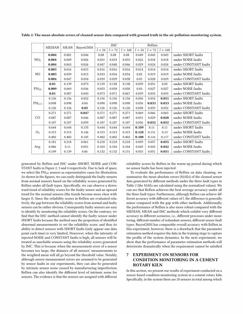
Table 2: The mean absolute errors of cleaned sensor data compared with ground truth in the air pollution monitoring system.

MEDIAN MEAN BayesGMM IMC RelSenl = 24 l = 72 l = 168 l = 24 l = 72 l = 168

NO2

0.004 0.081 0.044 0.08 0.08 0.08 0.049 0.045 0.043 under SHORT faults0.004 0.049 0.026 0.031 0.033 0.033 0.022 0.018 0.018 under NOISE faults0.004 0.063 0.026 0.047 0.048 0.046 0.029 0.024 0.024 under CONSTANT faults

NO0.003 0.016 0.015 0.016 0.016 0.016 0.014 0.014 0.014 under SHORT faults0.003 0.039 0.015 0.033 0.034 0.034 0.02 0.019 0.019 under NOISE faults0.004 0.047 0.034 0.039 0.039 0.038 0.03 0.028 0.029 under CONSTANT faults

PM10

0.01 0.139 0.073 0.139 0.138 0.138 0.059 0.051 0.05 under SHORT faults0.009 0.069 0.036 0.055 0.058 0.058 0.03 0.027 0.027 under NOISE faults0.01 0.087 0.043 0.073 0.071 0.067 0.039 0.033 0.033 under CONSTANT faults

PM2.5

0.156 0.156 0.052 0.156 0.156 0.156 0.056 0.054 0.051 under SHORT faults0.098 0.098 0.04 0.098 0.098 0.098 0.036 0.033 0.033 under NOISE faults0.126 0.126 0.05 0.126 0.126 0.126 0.058 0.053 0.052 under CONSTANT faults

CO0.271 0.271 0.047 0.271 0.271 0.271 0.069 0.066 0.063 under SHORT faults0.087 0.087 0.046 0.087 0.087 0.087 0.031 0.029 0.028 under NOISE faults0.107 0.107 0.059 0.107 0.107 0.107 0.056 0.052 0.052 under CONSTANT faults

O3

0.644 0.644 0.135 0.644 0.644 0.644 0.109 0.11 0.11 under SHORT faults0.315 0.315 0.146 0.315 0.315 0.315 0.128 0.131 0.13 under NOISE faults0.402 0.402 0.145 0.402 0.402 0.402 0.108 0.116 0.117 under CONSTANT faults

Avg.0.181 0.218 0.061 0.218 0.218 0.218 0.059 0.057 0.055 under SHORT faults0.086 0.11 0.051 0.103 0.104 0.104 0.045 0.043 0.042 under NOISE faults0.109 0.139 0.06 0.132 0.132 0.131 0.053 0.051 0.051 under CONSTANT faults

generated by RelSen and IMC under SHORT, NOISE and CON-STANT faults in Figure 2, 3 and 4 respectively. Due to lack of space,we select the PM10 sensors as representative cases for illustration.As shown in the figures, we can easily distinguish the faulty sensorsfrom normal sensors based on the reliability scores generated byRelSen under all fault types. Specifically, we can observe a down-ward trend of reliability scores for the faulty sensor and an upwardtrend for the normal sensors (the trends become more clear withlarger l). Since the reliability scores in RelSen are evaluated rela-tively, the gap between the reliability scores from normal and faultysensors can be rather obvious. Consequently faulty sensors are easyto identify by monitoring the reliability scores. On the contrary, wefind that the IMC method cannot identify the faulty sensor underSHORT faults because the method uses the proportion of identifiedabnormal measurements to set the reliability score, and thus itsability to detect sensors with SHORT faults (only appear one datapoint each time) is very limited. Moreover, when the intensity ofinjected NOISE and CONSTANT faults is high, all sensors will betreated as unreliable sensors using the reliability scores generatedby IMC. This is because when the measurement error of a sensorbecomes too large, the distance of all sensors’ measurements tothe weighted mean will all go beyond the threshold value. Notably,although sensor measurement errors are assumed to be generatedby sensor faults in our experiments, they can also be generatedby intrinsic sensor noise caused by manufacturing imperfection.RelSen can also identify the different level of intrinsic noise forsensors. The evidence is that the sensors are assigned with different

reliability scores by RelSen in the warm-up period during whichno sensor faults has been injected.

To evaluate the performance of RelSen on data cleaning, wesummarize the mean absolute errors (MAEs) of the cleaned sensordata generated by different methods under the three fault types inTable 2 (the MAEs are calculated using the normalized values). Wecan see that RelSen achieves the best average accuracy under allthe three fault types. Furthermore, although RelSen can achieve dif-ferent accuracy with different values of l , the difference is generallyminor compared with the gap with other methods. Additionally,the performance of RelSen is also more robust compared with theMEDIAN, MEAN and IMC methods which exhibit very differentaccuracy in different scenarios, i.e., different processes under moni-toring, different number of redundant sensors, different sensor faulttypes. BayesGMM has comparable overall accuracy with RelSen inthis experiment, however, there is a drawback that the parameterestimation method requires the data in the training stage to capturethe profile of the system dynamics. In the next experiment, weshow that the performance of parameter estimation methods willdeteriorate dramatically when the requirement cannot be satisfied.

7 EXPERIMENT ON SENSORS FORCONDITION MONITORING IN A CEMENTROTARY KILN

In this section, we present our results of experiment conducted on asensor-based condition monitoring system in a cement rotary kiln.Specifically, in the system there are 20 sensors in total among which

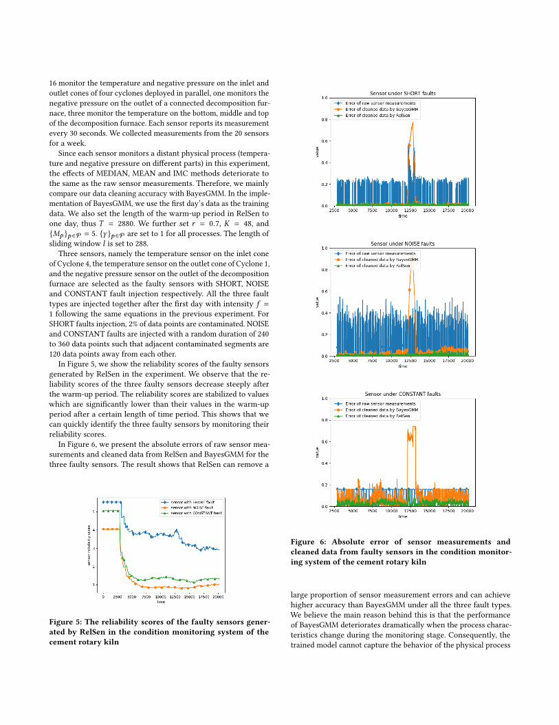
16 monitor the temperature and negative pressure on the inlet andoutlet cones of four cyclones deployed in parallel, one monitors thenegative pressure on the outlet of a connected decomposition fur-nace, three monitor the temperature on the bottom, middle and topof the decomposition furnace. Each sensor reports its measurementevery 30 seconds. We collected measurements from the 20 sensorsfor a week.

Since each sensor monitors a distant physical process (tempera-ture and negative pressure on different parts) in this experiment,the effects of MEDIAN, MEAN and IMC methods deteriorate tothe same as the raw sensor measurements. Therefore, we mainlycompare our data cleaning accuracy with BayesGMM. In the imple-mentation of BayesGMM, we use the first day’s data as the trainingdata. We also set the length of the warm-up period in RelSen toone day, thus T = 2880. We further set r = 0.7, K = 48, and{Mp }p∈P = 5. {γ }p∈P are set to 1 for all processes. The length ofsliding window l is set to 288.

Three sensors, namely the temperature sensor on the inlet coneof Cyclone 4, the temperature sensor on the outlet cone of Cyclone 1,and the negative pressure sensor on the outlet of the decompositionfurnace are selected as the faulty sensors with SHORT, NOISEand CONSTANT fault injection respectively. All the three faulttypes are injected together after the first day with intensity f =1 following the same equations in the previous experiment. ForSHORT faults injection, 2% of data points are contaminated. NOISEand CONSTANT faults are injected with a random duration of 240to 360 data points such that adjacent contaminated segments are120 data points away from each other.

In Figure 5, we show the reliability scores of the faulty sensorsgenerated by RelSen in the experiment. We observe that the re-liability scores of the three faulty sensors decrease steeply afterthe warm-up period. The reliability scores are stabilized to valueswhich are significantly lower than their values in the warm-upperiod after a certain length of time period. This shows that wecan quickly identify the three faulty sensors by monitoring theirreliability scores.

In Figure 6, we present the absolute errors of raw sensor mea-surements and cleaned data from RelSen and BayesGMM for thethree faulty sensors. The result shows that RelSen can remove a

Figure 5: The reliability scores of the faulty sensors gener-ated by RelSen in the condition monitoring system of thecement rotary kiln

Figure 6: Absolute error of sensor measurements andcleaned data from faulty sensors in the condition monitor-ing system of the cement rotary kiln

large proportion of sensor measurement errors and can achievehigher accuracy than BayesGMM under all the three fault types.We believe the main reason behind this is that the performanceof BayesGMM deteriorates dramatically when the process charac-teristics change during the monitoring stage. Consequently, thetrained model cannot capture the behavior of the physical process

any more. The evidence is clear in Figure 6, where BayesGMMfails to capture the dynamics of the physical processes around timepoints between 12000 to 13000. However, in RelSen we use randomlocal linear regression for soft sensor construction, this allows thesoft sensors to be promptly adapted to capture changing processcharacteristics, thus the estimated ground truth of process statesare more accurate.

8 CONCLUSIONIn this paper, we have proposed RelSen: a novel optimization-basedframework for simultaneous sensor reliability monitoring and datacleaning in sensor systems. The main logic behind RelSen is fairlystraightforward: more reliable sensors should provide more accu-rate measurements; the ground truth of monitored process statesshould be closer to themeasurements frommore reliable sensors. Byutilizing the cross correlation between multiple processes, RelSencan dynamically update the reliability scores of sensors and accu-rately clean sensor data in real time only given the measurementsfrom sensors. In our experiments conducted respectively on sensorsystems for outdoor air quality monitoring and cement rotary kilncondition monitoring, we demonstrated that RelSen can accuratelyand promptly identify unreliable sensors under three types of com-monly observed sensor faults. Furthermore, we showed that RelSenoutperformed several baseline methods regarding to data cleaning.

With less assumptions and knowledge requirements about themonitored process dynamics, we see potential for application ofRelSen to a wide range of use-cases in the sensor-based IoT applica-tions. In the future, we will study the potential to extend RelSen toa broader class of problems such as time-series data cleaning andmodel fusion in time-series ensemble learning.

REFERENCES[1] Charles K Chui, Guanrong Chen, et al. 2017. Kalman Filtering. Springer.[2] Pierre Del Moral. 1996. Non-linear Filtering: Interacting Particle Resolution.

Markov processes and related fields 2, 4 (1996), 555–581.[3] Arthur PDempster, NanMLaird, andDonald B Rubin. 1977. MaximumLikelihood

from Incomplete Data via the EM Algorithm. Journal of the Royal StatisticalSociety: Series B (Methodological) 39, 1 (1977), 1–22.

[4] Maya R Gupta, Eric K Garcia, and Erika Chin. 2008. Adaptive Local LinearRegression with Application to Printer Color Management. IEEE Transactions onImage Processing 17, 6 (2008), 936–945.

[5] Fredrik Gustafsson. 2010. Statistical Sensor Fusion. Studentlitteratur.[6] Andrew H Jazwinski. 1970. Stochastic Processes and Filtering Theory. Vol. 64.

Academic Press.[7] Simon J Julier and Jeffrey K Uhlmann. 2004. Unscented Filtering and Nonlinear

Estimation. Proc. IEEE 92, 3 (2004), 401–422.[8] Manabu Kano and Koichi Fujiwara. 2013. Virtual Sensing Technology in Process

Industries: Trends and Challenges Revealed by Recent Industrial Applications.JOURNAL OF CHEMICAL ENGINEERING OF JAPAN 46, 1 (2013), 1–17.

[9] Christine Keribin. 2000. Consistent Estimation of the Order of Mixture Models.Sankhya: The Indian Journal of Statistics, Series A (2000), 49–66.

[10] Prashant Kumar, Lidia Morawska, Claudio Martani, George Biskos, Marina Neo-phytou, Silvana Di Sabatino, Margaret Bell, Leslie Norford, and Rex Britter. 2015.The Rise of Low-cost Sensing for Managing Air Pollution in Cities. EnvironmentInternational 75 (2015), 199–205.

[11] Qi Li, Yaliang Li, Jing Gao, Lu Su, Bo Zhao, Murat Demirbas, Wei Fan, and JiaweiHan. 2014. A Confidence-aware Approach for Truth Discovery on Long-tail Data.Proceedings of the VLDB Endowment 8, 4 (2014), 425–436.

[12] Qi Li, Yaliang Li, Jing Gao, Bo Zhao, Wei Fan, and Jiawei Han. 2014. ResolvingConflicts in Heterogeneous Data by Truth Discovery and Source ReliabilityEstimation. In Proceedings of the 2014 ACM SIGMOD international conference onManagement of data. ACM, 1187–1198.

[13] Wangyan Li, Zidong Wang, Guoliang Wei, Lifeng Ma, Jun Hu, and Derui Ding.2015. A Survey on Multisensor Fusion and Consensus Filtering for SensorNetworks. Discrete Dynamics in Nature and Society 2015 (2015).

[14] Yaliang Li, Jing Gao, Chuishi Meng, Qi Li, Lu Su, Bo Zhao, Wei Fan, and JiaweiHan. 2016. A Survey on Truth Discovery. ACM Sigkdd Explorations Newsletter17, 2 (2016), 1–16.

[15] Yaliang Li, Qi Li, Jing Gao, Lu Su, Bo Zhao, Wei Fan, and Jiawei Han. 2015. On theDiscovery of Evolving Truth. In Proceedings of the 21th ACM SIGKDD InternationalConference on Knowledge Discovery and Data Mining. ACM, 675–684.

[16] Zhong-Xian Li, Xiao-Ming Yang, and Zongjin Li. 2006. Application of Cement-based Piezoelectric Sensors for Monitoring Traffic Flows. Journal of Transporta-tion Engineering 132, 7 (2006), 565–573.

[17] Lennart Ljung. 1999. System Identification. Wiley Encyclopedia of Electrical andElectronics Engineering (1999), 1–19.

[18] Chenyang Lu, Abusayeed Saifullah, Bo Li, Mo Sha, Humberto Gonzalez, DolvaraGunatilaka, Chengjie Wu, Lanshun Nie, and Yixin Chen. 2015. Real-timeWirelessSensor-actuator Networks for Industrial Cyber-physical Systems. Proc. IEEE 104,5 (2015), 1013–1024.

[19] Jeff Pasternack and Dan Roth. 2010. Knowing What to Believe (When YouAlready Know Something). In Proceedings of the 23rd International Conference onComputational Linguistics. Association for Computational Linguistics, 877–885.

[20] Jeff Pasternack and Dan Roth. 2011. Making Better Informed Trust Decisionswith Generalized Fact-finding. In Twenty-Second International Joint Conferenceon Artificial Intelligence.

[21] Jeff Pasternack and Dan Roth. 2013. Latent Credibility Analysis. In Proceedingsof the 22nd international conference on World Wide Web. ACM, 1009–1020.

[22] Giovanni Petris, Sonia Petrone, and Patrizia Campagnoli. 2009. Dynamic LinearModels. In Dynamic Linear Models with R. Springer, 31–84.

[23] Abhishek B Sharma, Leana Golubchik, and Ramesh Govindan. 2010. Sensor Faults:Detection Methods and Prevalence in Real-world Datasets. ACM Transactions onSensor Networks 6, 3 (2010), 23.

[24] Shuli Sun, Honglei Lin, Jing Ma, and Xiuying Li. 2017. Multi-sensor DistributedFusion Estimation with Applications in Networked Systems: A Review Paper.Information Fusion 38 (2017), 122–134.

[25] Rudolph Van Der Merwe, Arnaud Doucet, Nando De Freitas, and Eric A Wan.2001. The Unscented Particle Filter. In Advances in neural information processingsystems. 584–590.

[26] Dong Wang, Lance Kaplan, Hieu Le, and Tarek Abdelzaher. 2012. On TruthDiscovery in Social Sensing: A Maximum Likelihood Estimation Approach. InProceedings of the 11th international conference on Information Processing in SensorNetworks. 233–244.

[27] Hongkai Wen, Zhuoling Xiao, Andrew Markham, and Niki Trigoni. 2014. Accu-racy Estimation for Sensor Systems. IEEE Transactions on Mobile Computing 14,7 (2014), 1330–1343.

[28] Hongkai Wen, Zhuoling Xiao, Niki Trigoni, and Phil Blunsom. 2013. On Assess-ing the Accuracy of Positioning Systems in Indoor Environments. In EuropeanConference on Wireless Sensor Networks. Springer, 1–17.

[29] Yao-Jung Wen, Alice M Agogino, and Kai Goebel. 2004. Fuzzy Validation andFusion for Wireless Sensor Networks. In ASME 2004 International MechanicalEngineering Congress and Exposition. American Society of Mechanical EngineersDigital Collection, 727–732.

[30] Stephen J Wright. 2015. Coordinate Descent Algorithms. Mathematical Program-ming 151, 1 (2015), 3–34.

[31] Lin Xiao, Stephen Boyd, and Sanjay Lall. 2005. A Scheme for Robust DistributedSensor Fusion Based on Average Consensus. In Fourth International Symposiumon Information Processing in Sensor Networks. IEEE, 63–70.

[32] Chao Yuan and Claus Neubauer. 2007. Bayesian Sensor Estimation for MachineCondition Monitoring. In 2007 IEEE International Conference on Acoustics, Speech,and Signal Processing. IEEE, 517–520.

[33] Chao Yuan and Claus Neubauer. 2008. Robust Sensor Estimation Using TemporalInformation. In 2008 IEEE International Conference on Acoustics, Speech and SignalProcessing. IEEE, 2077–2080.

[34] Jiangfan Zhang, Rick S Blum, and Lance Kaplan. 2017. Cyber Attacks on Estima-tion Sensor Networks and IoTs: Impact, Mitigation and Implications to UnattackedSystems. In 2017 IEEE International Conference on Acoustics, Speech and SignalProcessing. IEEE, 3316–3320.

[35] Ridong Zhang, Sheng Wu, and Furong Gao. 2017. State Space Model PredictiveControl for Advanced Process Operation: a Review of Recent Development, Newresults, and Insight. Industrial & Engineering Chemistry Research 56, 18 (2017),5360–5394.

[36] Yihong Zhang, Claudia Szabo, and Quan Z Sheng. 2014. Cleaning EnvironmentalSensing Data Streams based on Individual Sensor Reliability. In InternationalConference on Web Information Systems Engineering. Springer, 405–414.

[37] Yihong Zhang, Claudia Szabo, and Quan Z Sheng. 2016. Reduce or Remove:Individual Sensor Reliability Profiling andData Cleaning. Intelligent Data Analysis20, 5 (2016), 979–995.

[38] Bo Zhao and Jiawei Han. 2012. A Probabilistic Model for Estimating Real-valuedTruth from Conflicting Sources. Proc. of QDB (2012).

[39] Zhanxing Zhu, Francesco Corona, Amaury Lendasse, Roberto Baratti, and Jose ARomagnoli. 2011. Local Linear Regression for Soft-sensor Designwith Applicationto an Industrial Deethanizer. IFAC Proceedings Volumes 44, 1 (2011), 2839–2844.