Reliable Predictive Computational Fluid Dynamics … · 1! Reliable Predictive Computational Fluid...
26
1 Reliable Predictive Computational Fluid Dynamics Models for Coal Gasifier Simulations with Uncertainty Quantification Performance Measures x.x, x.x, and x.x Aytekin Gel 1,2 , Mehrdad Shahnam 1 , Arun K. Subramaniyan 3 1 National Energy Technology Laboratory , Morgantown, WV, U.S.A. 2 ALPEMI Consulting LLC, Phoenix, AZ, U.S.A. 3 GE Global Research , U.S.A. 2013 NETL Workshop on Multiphase Flow Science Lakeview Resort, Morgantown, WV August 6 – 7, 2013
Transcript of Reliable Predictive Computational Fluid Dynamics … · 1! Reliable Predictive Computational Fluid...

1!
Reliable Predictive Computational Fluid Dynamics Models for Coal Gasifier Simulations with
Uncertainty Quantification
Performance Measures x.x, x.x, and x.x!
Aytekin Gel1,2 , Mehrdad Shahnam1, Arun K. Subramaniyan3
1 National Energy Technology Laboratory , Morgantown, WV, U.S.A.
2 ALPEMI Consulting LLC, Phoenix, AZ, U.S.A. 3 GE Global Research , U.S.A.
2013 NETL Workshop on Multiphase Flow Science Lakeview Resort, Morgantown, WV
August 6 – 7, 2013

2
Presentation Outline
§ Motivation and Objective § Overview of Uncertainty Quantification Frameworks § Results from Two Non-intrusive UQ Analysis Methods
• NETL’s B22 riser simulations § Summary & Conclusions § Future Work

3
Motivation and Objectives
§ Computational science and simulation based engineering (SBE) have become an indispensible tool for resolving complex engineering problems through simulation.
§ Reactive multiphase flow models and simulation tools (e.g., MFIX) play important role in development of new technologies for fossil fuel based clean energy.
§ Increasingly strong need for assessment of credibility of the predictions from simulations for wider acceptance of SBE.
§ Uncertainty quantification (UQ) methods provide a yardstick.
Objective: § Determine the best set of UQ methods and tools applicable for
reactive multiphase flow simulation.

4
Uncertain!inputs!
Quick Overview of Uncertainty Quantification (UQ) Methods
Intrusive UQ Several Available Methods: § Polynomial Chaos Expansions
(PCE) § Stochastic Expansion Pro: § Quick prediction Con: § Surgery in the code and long
development time
Non-Intrusive UQ Several Available Methods: § Surrogate Model + Monte Carlo § Polynomial Chaos Expansions § Bayesian Techniques Pro: § Short development time Con: § Sampling error
Stochastic simulation!(UQ embedded in the model)!
Uncertainty!information!Model!
Uncertain!inputs!
UQ Toolbox!
Model!
UQ achieved by sampling !many deterministic simulations!
Source: An Introduction to Uncertainty Quantification Methodologies and Methods, C. Tong (2012) & Comparing Uncertainty Quantification Methods Under Practical Industry Requirements, Wang (2012)

5
Questions Addressed with Uncertainty Quantification: § What is the effect of variability in system input on the quantities of
interest (QoI)? E.g. How is the gasifier yield affected from operating condition variability or batch to batch coal feed variations? è Forward Propagation of Input Uncertainties
• Which input contributes most to variability of QoI? E.g. If the variability in yield of gasifier output exceeds the allowable process limits, which system input factor needs to be managed or investigated to reduce uncertainty. è Sensitivity Analysis
• How to use observed data to calibrate system parameters? è Bayesian Calibration
§ What is the uncertainty in CFD simulation based predictions for scale-up studies? è Total Prediction Uncertainty Quantification
Several Questions To Be Addressed By Using Non-intrusive Uncertainty Quantification and Propagation In Our Simulations?

6
Demonstration of applicability of UQ methods in answering questions through representative problems: § Case A: 3D Transient Fluidized Bed Riser Simulation
• Non-reacting multiphase flow simulation with MFiX • B-22 riser at NETL with experimental data from 2010 NETL/
PSRI Fluidization Challenge Problem.
§ Case B: 2D Transient Gasifier Simulation • Reacting multiphase flow simulation with MFiX
§ Case C: 3D Transient Fluidized Bed Gasifier • Reacting multiphase flow simulation with Fluent • UQ compatible experimental data from Canadian collaborators
Non-Intrusive UQ Methodology Demonstration Results

7
Case A: 3D Transient Fluidized Bed Riser Simulation (in collaboration with T. Li, B. Gopalan, M. Syamlal)
B22 riser schematic illustration!
Enlarged view of the!simulated section!
Uncertainty Quantification Study Properties: Input parameters with Uncertainty [min-max range]: (1) Superficial gas velocity (m/s): [7.2 – 8.12] (2) Gas flow through distributor (kg/s) [12.6 – 15.98] Quantity of Interest: Pressure Drop (kPa)
Sampling Method: Central Composite Sample Size = 13 Computational time/sample: ~22 days on 80 cores
Publication Reference:!Gel, A., Li, T., Gopalan, B., Shahnam, M., Syamlal, M., “Validation and Uncertainty Quantification of a Multiphase CFD Model”, Industrial & Engineering Chemistry Research, (2013) http://pubs.acs.org/doi/abs/10.1021/ie303469f.!
8
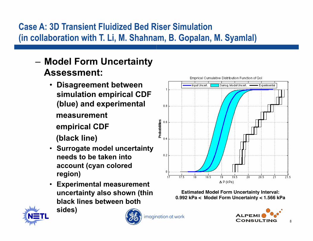
– Model Form Uncertainty Assessment:
• Disagreement between simulation empirical CDF (blue) and experimental
measurement empirical CDF (black line) • Surrogate model uncertainty
needs to be taken into account (cyan colored region)
• Experimental measurement uncertainty also shown (thin black lines between both sides)
Estimated Model Form Uncertainty Interval:!0.992 kPa < Model Form Uncertainty < 1.566 kPa!
Case A: 3D Transient Fluidized Bed Riser Simulation (in collaboration with T. Li, M. Shahnam, B. Gopalan, M. Syamlal)
9
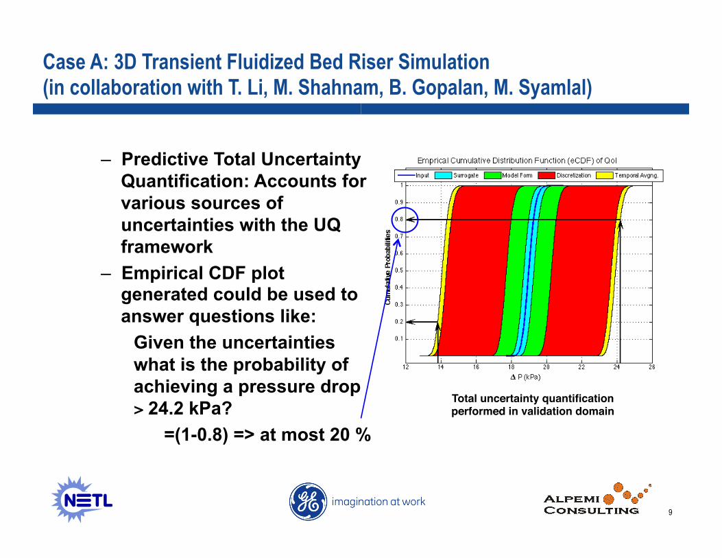
– Predictive Total Uncertainty Quantification: Accounts for various sources of uncertainties with the UQ framework
– Empirical CDF plot generated could be used to answer questions like:
Given the uncertainties what is the probability of achieving a pressure drop > 24.2 kPa? =(1-0.8) => at most 20 %
Total uncertainty quantification performed in validation domain!
Case A: 3D Transient Fluidized Bed Riser Simulation (in collaboration with T. Li, M. Shahnam, B. Gopalan, M. Syamlal)

10
Preliminary Results of Alternate UQ framework for Same Data Bayesian Analysis for Case A: Global Sensitivity Analysis
– Which input parameter contributes most to the variability observed in the quantity of interest, dP?
• Gs ~ 60% • Ug ~ 39% • Interaction of Gs & Ug < 1%
– Primarily main effects
11
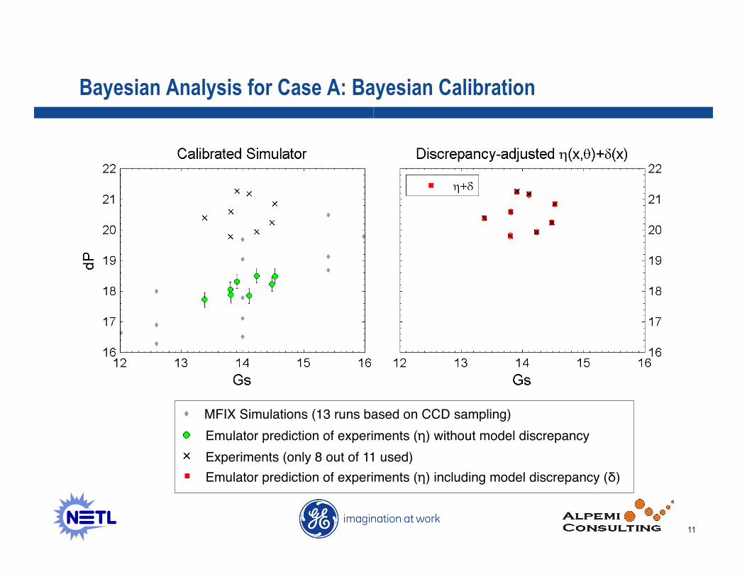
Bayesian Analysis for Case A: Bayesian Calibration
MFIX Simulations (13 runs based on CCD sampling)"Emulator prediction of experiments (η) without model discrepancy "Experiments (only 8 out of 11 used)"Emulator prediction of experiments (η) including model discrepancy (δ) "
12
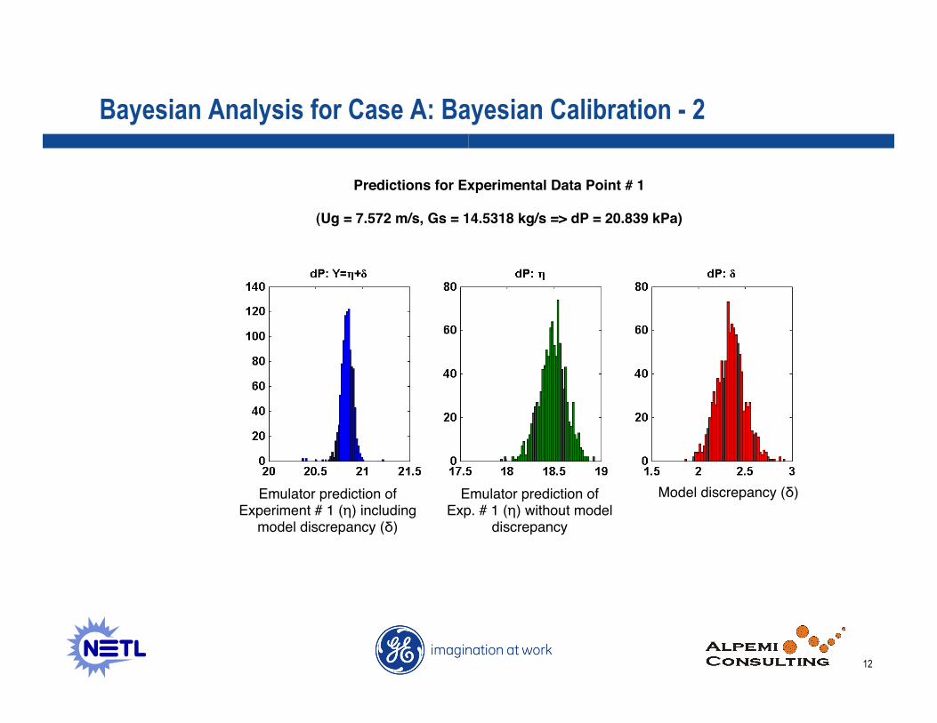
Bayesian Analysis for Case A: Bayesian Calibration - 2
Predictions for Experimental Data Point # 1!!
(Ug = 7.572 m/s, Gs = 14.5318 kg/s => dP = 20.839 kPa)! !
Emulator prediction of "Exp. # 1 (η) without model
discrepancy "
Emulator prediction of "Experiment # 1 (η) including "
model discrepancy (δ) "
Model discrepancy (δ) "

13
Summary and Conclusions
§ Exploring different UQ techniques to identify those that are best suited for reacting multiphase flows.
§ Non-intrusive UQ enables black box treatment of the application code but requires adequate samples to achieve the necessary accuracy by reducing sampling error.
§ Typically 80% of effort spent goes into constructing an adequate surrogate model.
§ Bayesian methods appears to offer various favorable features such as quantification of model discrepancy and inclusion of prior information, which can be used effectively to alleviate lack of data.
14
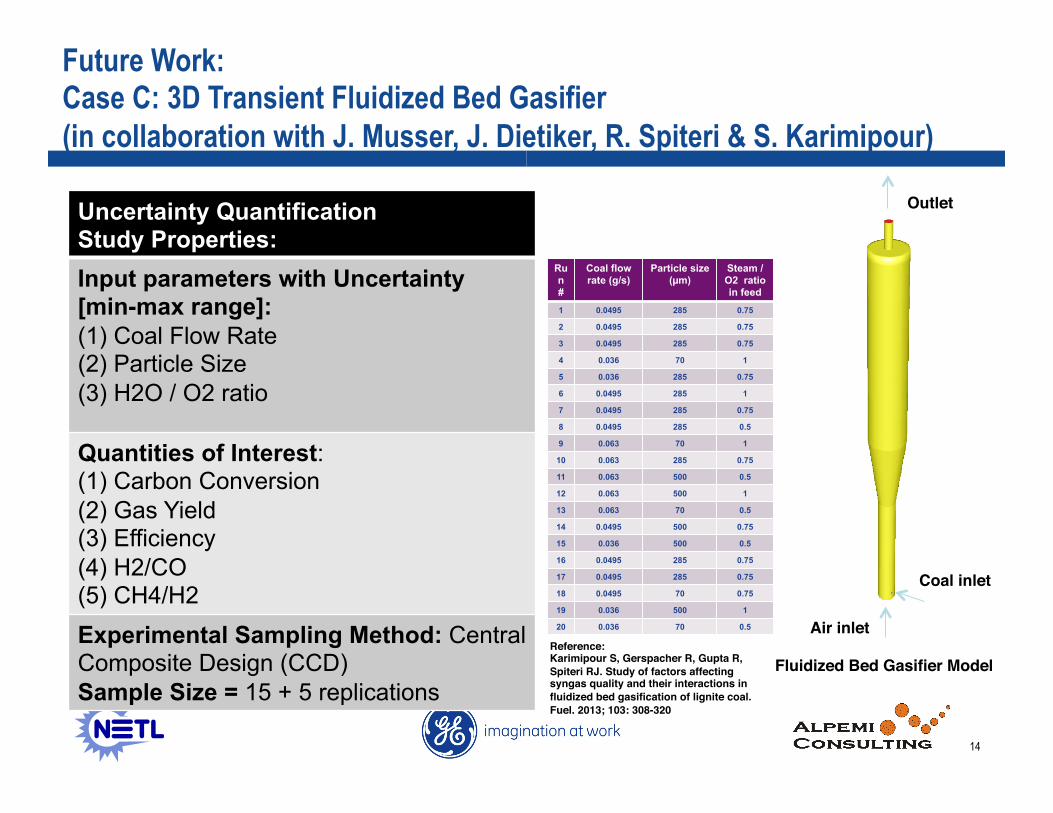
Future Work: Case C: 3D Transient Fluidized Bed Gasifier (in collaboration with J. Musser, J. Dietiker, R. Spiteri & S. Karimipour)
Fluidized Bed Gasifier Model!
Uncertainty Quantification Study Properties: Input parameters with Uncertainty [min-max range]: (1) Coal Flow Rate (2) Particle Size (3) H2O / O2 ratio
Quantities of Interest: (1) Carbon Conversion (2) Gas Yield (3) Efficiency (4) H2/CO (5) CH4/H2 Experimental Sampling Method: Central Composite Design (CCD) Sample Size = 15 + 5 replications
Coal inlet!
Air inlet!
Outlet!
Run #
Coal flow rate (g/s)
Particle size (!m)
Steam /O2 ratio in feed
1 0.0495 285 0.75
2 0.0495 285 0.75
3 0.0495 285 0.75
4 0.036 70 1
5 0.036 285 0.75
6 0.0495 285 1
7 0.0495 285 0.75
8 0.0495 285 0.5
9 0.063 70 1
10 0.063 285 0.75
11 0.063 500 0.5
12 0.063 500 1
13 0.063 70 0.5
14 0.0495 500 0.75
15 0.036 500 0.5
16 0.0495 285 0.75
17 0.0495 285 0.75
18 0.0495 70 0.75
19 0.036 500 1
20 0.036 70 0.5
Reference:!Karimipour S, Gerspacher R, Gupta R, Spiteri RJ. Study of factors affecting syngas quality and their interactions in fluidized bed gasification of lignite coal. Fuel. 2013; 103: 308-320!

15
• Initial analysis of the experimental results with Bayesian framework performed
E.g., global sensitivity analysis for Carbon Conversion
Case C: 3D Transient Fluidized Bed Gasifier (in collaboration with J. Musser, J. Dietiker, R. Spiteri & S. Karimipour)

16
Thank you for your attention. Questions?
Acknowledgments: Dr. Charles Tong, CASC, Lawrence Livermore National Laboratory (LLNL). This technical effort was performed in support of the National Energy Technology Laboratory’s ongoing research in multiphase flows under the RDS contract DE-AC26-04NT41817 and RES contract DE-FE0004000.
Volume rendering visualizations of first-of-its-kind
commercial scale gasifier simulation on Cray XT6
at OLCF by A. Gel.

17
Additional
Slides
18
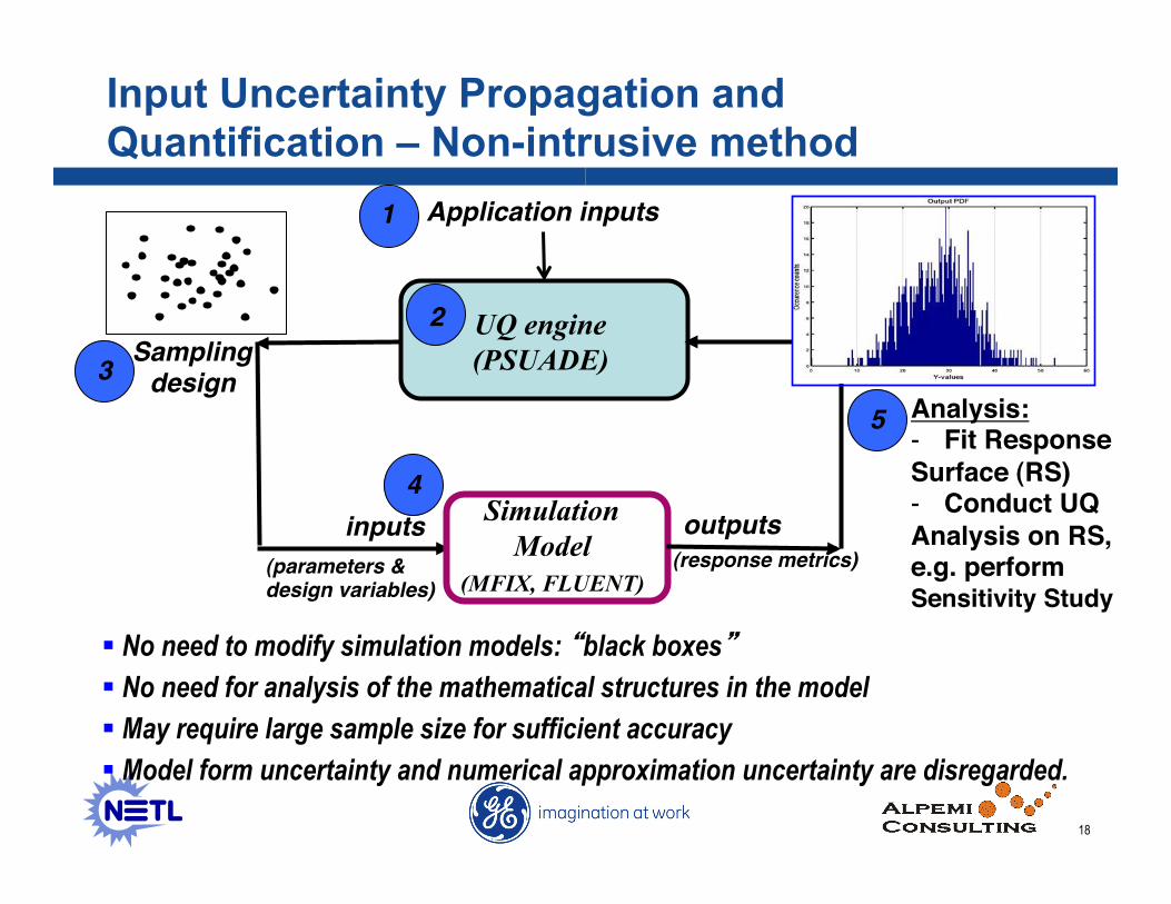
Simulation Model
(MFIX, FLUENT)
Sampling!design!
UQ engine (PSUADE)
Analysis:!- Fit Response!Surface (RS)!- Conduct UQ !Analysis on RS, !e.g. perform !Sensitivity Study!
outputs!inputs!
Application inputs!
§ No need to modify simulation models: “black boxes” § No need for analysis of the mathematical structures in the model § May require large sample size for sufficient accuracy § Model form uncertainty and numerical approximation uncertainty are disregarded.
(parameters &!design variables)!
(response metrics)!
1!
2!
3!
4!
5!
Input Uncertainty Propagation and Quantification – Non-intrusive method

19
Accomplishments – UQ (Case A)
§ Case A: 3D Transient Fluidized Bed Riser Simulation Objective: Assess total uncertainty using a comprehensive VUQ framework by Roy & Oberkampf
Grid Resolution Coarse 25 x 1050 x 19 Medium 35 x 1485 x 27 Fine 50 x 2100 x 38
B22 riser schematic illustration!
Enlarged view of the!simulated section!
20
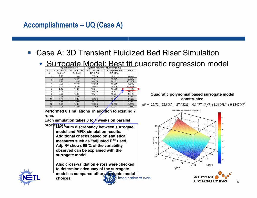
Accomplishments – UQ (Case A)
§ Case A: 3D Transient Fluidized Bed Riser Simulation • Surrogate Model: Best fit quadratic regression model
Maximum discrepancy between surrogate model and MFIX simulation results. !Additional checks based on statistical measures such as “adjusted R2” used. Adj. R2 shows 98 % of the variability observed can be explained with the surrogate model.! !Also cross-validation errors were checked to determine adequacy of the surrogate model as compared other surrogate model choices. !
Performed 6 simulations in addition to existing 7 runs.!Each simulation takes 3 to 4 weeks on parallel processors!
Quadratic polynomial based surrogate model constructed!
for Quantity Of Interest: Pressure Drop (kPA)!

21
Bayesian Analysis for Case A: 1D Uncertainty w.r.t. Ug & Gs
– At any point of Ug, (e.g. Ug = 8 m/s) the plotted uncertainty in dP is due to variation in Gs over it’s entire range, i.e., 12.02 – 15.98 kg/s, which is obtained by integrating along Gs.
22
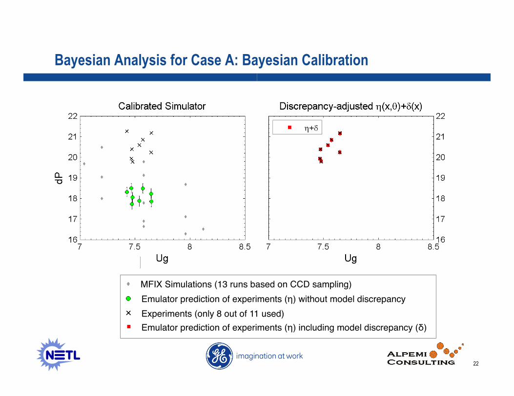
Bayesian Analysis for Case A: Bayesian Calibration
MFIX Simulations (13 runs based on CCD sampling)"Emulator prediction of experiments (η) without model discrepancy "Experiments (only 8 out of 11 used)"Emulator prediction of experiments (η) including model discrepancy (δ) "
23
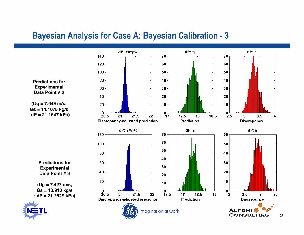
Bayesian Analysis for Case A: Bayesian Calibration - 3
Predictions for Experimental !Data Point # 2 !
!(Ug = 7.649 m/s, !
Gs = 14.1075 kg/s !: dP = 21.1647 kPa)!
!
Predictions for Experimental !Data Point # 3!
!(Ug = 7.427 m/s, !Gs = 13.913 kg/s !
: dP = 21.2529 kPa) !

24
Bayesian Analysis for Case A: Bayesian Calibration - 3
Predictions for Experimental !Data Point # 4 !
!(Ug = 7.648 m/s, !
Gs = 14.2348 kg/s !: dP = 19.9257 kPa)!
!
Predictions for Experimental !Data Point # 5!
!(Ug = 7.54 m/s, !
Gs = 13.813 kg/s !: dP = 20.5865 kPa) !

25
Bayesian Analysis for Case A: Bayesian Calibration - 3
Predictions for Experimental !Data Point # 6 !
!(Ug = 7.472 m/s, !
Gs = 13.3843 kg/s !: dP = 20.3883 kPa)!
!
Predictions for Experimental !Data Point # 7!
!(Ug = 7.479 m/s, !
Gs = 13.8039 kg/s !: dP = 19.7741 kPa) !
26
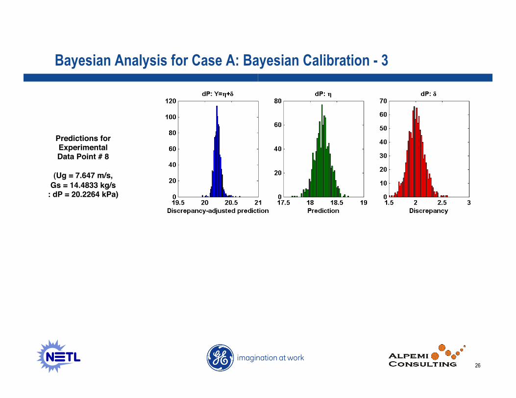
Bayesian Analysis for Case A: Bayesian Calibration - 3
Predictions for Experimental !Data Point # 8 !
!(Ug = 7.647 m/s, !
Gs = 14.4833 kg/s !: dP = 20.2264 kPa)!
!