Reliable, Low Cost Distributed Generator/Utility System Interconnect ... · GE Corporate Research...

August 2003 • NREL/SR-560-34634

GE Corporate Research and Development Niskayuna, New York

Reliable, Low Cost Distributed Generator/Utility System Interconnect 2001 Annual Report

National Renewable Energy Laboratory 1617 Cole Boulevard Golden, Colorado 80401-3393 NREL is a U.S. Department of Energy Laboratory Operated by Midwest Research Institute • Battelle • Bechtel

Contract No. DE-AC36-99-GO10337

August 2003 • NREL/SR-560-34634

Reliable, Low Cost Distributed Generator/Utility System Interconnect 2001 Annual Report

GE Corporate Research and Development Niskayuna, New York

NREL Technical Monitor: B. Kroposki Prepared under Subcontract No. NAD-1-30605-01

National Renewable Energy Laboratory 1617 Cole Boulevard Golden, Colorado 80401-3393 NREL is a U.S. Department of Energy Laboratory Operated by Midwest Research Institute • Battelle • Bechtel

Contract No. DE-AC36-99-GO10337

This publication was reproduced from the best available copy

Submitted by the subcontractor and received no editorial review at NREL NOTICE This report was prepared as an account of work sponsored by an agency of the United States government. Neither the United States government nor any agency thereof, nor any of their employees, makes any warranty, express or implied, or assumes any legal liability or responsibility for the accuracy, completeness, or usefulness of any information, apparatus, product, or process disclosed, or represents that its use would not infringe privately owned rights. Reference herein to any specific commercial product, process, or service by trade name, trademark, manufacturer, or otherwise does not necessarily constitute or imply its endorsement, recommendation, or favoring by the United States government or any agency thereof. The views and opinions of authors expressed herein do not necessarily state or reflect those of the United States government or any agency thereof.

Available electronically at http://www.osti.gov/bridge

Available for a processing fee to U.S. Department of Energy and its contractors, in paper, from:

U.S. Department of Energy Office of Scientific and Technical Information P.O. Box 62 Oak Ridge, TN 37831-0062 phone: 865.576.8401 fax: 865.576.5728 email: [email protected]

Available for sale to the public, in paper, from:

U.S. Department of Commerce National Technical Information Service 5285 Port Royal Road Springfield, VA 22161 phone: 800.553.6847 fax: 703.605.6900 email: [email protected] online ordering: http://www.ntis.gov/ordering.htm

Printed on paper containing at least 50% wastepaper, including 20% postconsumer waste

http://www.osti.gov/bridge

http://www.ntis.gov/ordering.htm

i

Contents Executive Summary......................................................................................................................... 1

1. Introduction ............................................................................................................................. 3 1.1. Objective.......................................................................................................................... 3 1.2. Technical Approach....................................................................................................... 3

1.2.1. Virtual Test Bed........................................................................................................... 3 1.2.2. Case Studies................................................................................................................. 3 1.2.3. Conceptual Interconnect Design................................................................................. 4

2. Virtual Test Bed........................................................................................................................ 5 2.1. Two Complementary Virtual Test Bed Platforms............................................................ 5

2.1.1. PSLF Description......................................................................................................... 5 2.1.2. Saber Description........................................................................................................ 5 2.1.3. Integration Approach.................................................................................................. 5

2.2. Models Development....................................................................................................... 6 2.2.1. Model Complexity Levels ............................................................................................ 6 2.2.2. PSLF Models................................................................................................................ 6

2.2.2.1. PSLF DG Models.................................................................................................. 6 2.2.2.2. PSLF EPS Models................................................................................................. 7 2.2.2.3. PSLF Load Models............................................................................................... 7

2.2.3. Saber Models ............................................................................................................... 7 2.2.3.1. Saber DG Models................................................................................................. 7 2.2.3.2. Saber EPS Models................................................................................................ 8 2.2.3.3. Saber Load Models.............................................................................................. 8

2.3. Virtual Test Bed Setups................................................................................................... 9 2.3.1. PSLF VTB Setups....................................................................................................... 10

2.3.1.1. PSLF Setup P1 ................................................................................................... 10 2.3.1.2. PSLF Setup P2 ................................................................................................... 11 2.3.1.3. PSLF Setup P3 ................................................................................................... 15

2.3.2. Saber VTB Setups...................................................................................................... 22 2.3.2.1. Saber Setup S1 ................................................................................................... 22 2.3.2.2. Saber Setup S2 ................................................................................................... 22 2.3.2.3. Saber Setup S3 ................................................................................................... 23

2.4. Summary....................................................................................................................... 24

3. Case Studies............................................................................................................................ 25 3.1. Power Quality Case Studies ........................................................................................... 25

3.1.1. Voltage Regulation.................................................................................................... 25 3.1.1.1. Generic Radial Feeder Models and Cases for Voltage Regulation Analysis....... 26 3.1.1.2. Generic Feeder Voltage Regulation Results ...................................................... 29 3.1.1.3. P2 System Study................................................................................................. 30 3.1.1.4. Summary of Significant Voltage Regulation Issues ........................................... 35

3.1.2. DG Design Considerations to Meet Power Quality Requirements............................. 38 3.1.2.1. Current Distortion from Power Electronic DG.................................................. 38

ii

3.1.2.2. Flicker Concerns for DG.................................................................................... 39 3.1.2.3. DC Current Injection ........................................................................................ 45 3.1.2.4. DG Grounding Issue.......................................................................................... 45 3.1.2.5. Unbalanced Grid............................................................................................... 48 3.1.2.6. Summary........................................................................................................... 51

3.2. Protection and Reliability Case Studies......................................................................... 52 3.2.1. Transient Response and Fault Behaviors .................................................................. 52

3.2.1.1. Capacitor Switching .......................................................................................... 52 3.2.1.2. Fault Analysis..................................................................................................... 58 3.2.1.3. Summary........................................................................................................... 66 3.2.1.4. Conclusions ....................................................................................................... 67

3.2.2. Anti-Islanding Protection of DG................................................................................ 67 3.2.2.1. Analysis of Sandia Anti-Islanding Algorithm .................................................... 68 3.2.2.2. Implications of the Gains Settings of the Sandia Anti-Islanding Algorithm..... 71 3.2.2.3. Time-Domain Simulations................................................................................ 76 3.2.2.4. Summary........................................................................................................... 81

3.2.3. Reclosing ................................................................................................................... 82 3.2.3.1. Out of Phase Reclosing...................................................................................... 82 3.2.3.2. Summary........................................................................................................... 89

3.3. Power System Dynamics and Stability Case Studies....................................................... 89 3.3.1. Introductory Dynamics Discussion............................................................................ 89 3.3.2. Local Distribution System Stability Issues.................................................................. 90

3.3.2.1. Discussion of P2 System..................................................................................... 90 3.3.2.2. Local Voltage Behavior without High Level Controls ....................................... 91 3.3.2.3. Impact of Various Control on Local Dynamics................................................. 92 3.3.2.4. Impact of Various Anti-Islanding Functions on Local Dynamics...................... 93

3.3.3. Bulk System Stability Issues........................................................................................ 96 3.3.3.1. Impact of DG Penetration on Bulk System Dynamics....................................... 96 3.3.3.2. Impact of Anti-Islanding Schemes on Bulk System Dynamics........................... 98 3.3.3.3. Impact of DG Tripping on Bulk System Dynamics ......................................... 101

3.3.4. Microgrid Dynamics................................................................................................ 107 3.3.4.1. Microgrid Dynamics with Autonomous Controls............................................ 108 3.3.4.2. Microgrid Dynamics with Supervisory Control................................................ 114

3.3.5. Power System Dynamics Summary.......................................................................... 116 3.4. Summary..................................................................................................................... 116

4. Conceptual Interconnect Design.......................................................................................... 119 4.1. Introduction................................................................................................................ 119

4.1.1. Interconnect Needs and Issues ................................................................................ 119 4.1.2. Reliable and Low Cost Interconnect Solution......................................................... 119

4.2. DG and Interconnect Design Improvement................................................................ 120 4.2.1. Implications From Case Studies .............................................................................. 120

4.2.1.1. Power Quality Improvements.......................................................................... 120 4.2.1.2. Reliability and Protection Improvements........................................................ 124

4.2.2. Anti-Islanding Control ............................................................................................ 125 4.2.2.1. Background..................................................................................................... 126 4.2.2.2. Anti-Islanding Design Considerations............................................................. 127

iii

4.3. DG/EPS Interconnect Standards and Requirements.................................................. 128 4.3.1. Background............................................................................................................. 128 4.3.2. Common Requirements in Different Standards ..................................................... 129

4.3.2.1. Isolating Switch............................................................................................... 129 4.3.2.2. Protective Relays.............................................................................................. 130 4.3.2.3. Anti-Islanding.................................................................................................. 130 4.3.2.4. Synchronization .............................................................................................. 130 4.3.2.5. Power Quality and Harmonics........................................................................ 131 4.3.2.6. Grounding....................................................................................................... 131 4.3.2.7. Metering.......................................................................................................... 131 4.3.2.8. Fault Protection............................................................................................... 131 4.3.2.9. Others.............................................................................................................. 132

4.3.3. Dissimilarities among the Standards....................................................................... 132 4.3.3.1. Protective Relays.............................................................................................. 132 4.3.3.2. Dedicated Transformer................................................................................... 132 4.3.3.3. Reclosing ......................................................................................................... 133

4.3.4. Summary................................................................................................................. 133 4.4. Conceptual Interconnect Design................................................................................. 134

4.4.1. Current Interconnect Status.................................................................................... 134 4.4.1.1. Power-Carrying Devices ................................................................................... 134 4.4.1.2. Protection and Control Devices....................................................................... 134 4.4.1.3. Inverters........................................................................................................... 134

4.4.2. Future Interconnect Needs and Trends.................................................................. 136 4.4.2.1. Local Protection .............................................................................................. 137 4.4.2.2. Local Control................................................................................................... 138 4.4.2.3. Coordinated Protection and Control.............................................................. 138 4.4.2.4. Enterprise Energy Control............................................................................... 139 4.4.2.5. Commerce....................................................................................................... 140

4.4.3. Conceptual Interconnect Design............................................................................. 141 4.4.3.1. Interconnect Technology Roadmap............................................................... 141 4.4.3.2. Conceptual Design .......................................................................................... 143

4.4.4. Summary................................................................................................................. 146

5. Summary............................................................................................................................... 147

References ................................................................................................................................... 149

1

Executive Summary

In the future, power distribution systems

now controlled by large providers of power generation will be replaced by more distributed power generation architectures where the lines of demarcation between providers and users of power are less restrictive. The industry is apprehensive about how existing power distribution systems can accommodate such a changeover within the next 5-10 years. In addition, there is significant concern about how this changeover will affect the economics and performance of power delivery and even the implementation of new power distribution architectures and controls. One of the key issues is the distributed generation – electric power system (DG-EPS) interconnection, which has fundamental impacts on current EPS operation and future DG penetration (i.e. the fraction of system power provided by interconnected DGs).

The research program has developed requirements that support the definition, design, and demonstration of a DG-EPS interconnection interface concept that allows DG to be interconnected to the EPS in a manner that provides value to the end users without compromising reliability and performance.

The first phase of the program developed a virtual test bed (VTB), which is a simulation platform suite that includes EPS, DG, and load models. Utilizing the VTB, comprehensive case studies to evaluate power quality, protection, reliability and stability were conducted in the second phase of the program. In the third phase of the program, the case study results were used to support the requirements definition for a

DG-EPS interconnection interface, and a conceptual interconnect design.

The development of the VTB allowed for exploration of the ways that DGs interact with the EPS under wide range of realistic conditions. Using the VTB, DG and EPS response to such events as short circuits on power lines, line switching operations, and load fluctuations were examined. Impacts ranging from effects on local distribution feeders up to entire multi-GW interconnected power systems were considered. These explorations showed that as the penetration of DG increases, the performance requirements for the DG become broader. The ability to achieve the desired performance with an autonomous local interconnect become limited, and penalties for undesirable behavior, such as over-aggressive DG tripping, become greater.

The development of a universal interconnect can follow a natural progression of functionality. The basic requirements imposed by the various interconnection standards, most notably IEEE P1547, provide a foundation on which higher levels of functionality can be built. These higher levels of functionality benefit both system reliability and the economics of DG. Thus, the universality of the interconnection device should be viewed as a platform upon which the functions required to maximize the economic and performance benefits of DG can be built, rather than a single device that will allow all possible DG to be uniformly connected to any host electric power system.

This report will provide a detailed discussion of these points and the accomplishments of the three phases of the

Executive Summary

2

program. The report is organized into sections corresponding to the three phases of the project, i.e. virtual test bed development, case studies, and conceptual

interconnect design. Each of the phases includes a summary of key findings for that phase.

3

1. Introduction

1.1. Objective

Traditional non-utility generated power sources, such as emergency and standby power systems, have minimal interaction with the electric power system. As Distributed Generation (DG) hardware becomes more reliable and economically feasible, there is an increasing trend to interconnect those DG units with the existing utilities to meet various energy needs, as well as to offer more service possibilities to customers and the host Electric Power Systems (EPS). Among these services are (1) standby/backup power to improve availability and reliability of electric power; (2) peak load shaving; (3) combined heat and power; (4) the ability to sell power back to utilities or other users; (5) power quality, such as reactive power compensation and voltage support; and (6) dynamic stability support, to name a few. This trend is fueled and accelerated by utility deregulation.

However, a wide range of system issues arises when the DG units attempt to connect to the EPS. Major issues regarding the interconnection of DG include protection, power quality, system reliability and system operation. Another complex issue is interconnection cost, which involves equipment design, industry standards, and the local utility’s approval process. These are some of the issues that have been identified as barriers to the application of DG interconnected to the EPS [1]. The solutions to these technical challenges will help not only shape the future of electric power generation, transmission, and

distribution systems, but will also have a profound impact on the economics.

The objective of the program was to systematically address the above mentioned issues. The outcome of the study and analysis will provide input for IEEE P1547 standard development.

1.2. Technical Approach

The base year program, presented in this report, was structured in three stages: 1) virtual test bed development; 2) case studies; and 3) conceptual interconnect design.

1.2.1. Virtual Test Bed

The virtual test bed (VTB) utilizes two complementary simulation tools to study the DG-EPS interconnection issues. These tools are the GE Positive Sequence Load Flow (PSLF) program and the Saber program, both of which are commercially available. PSLF is an industry standard modeling tool for analyzing large-scale system response. Saber is a commercial mix-technology analog/digital signal simulator suitable for detailed component level modeling. The key features of the VTB include multiple complexity level component models that are scalable and expandable, plug-n-play capability, and the ability to provide validation against test results.

1.2.2. Case Studies

The set of simulations run on the VTB were based on a case list compiled by the team from various brainstorming sessions, IEEE P1547 Draft Standard for interconnecting Distributed Resources with Electric Power Systems [2], Edison Electric Institute Distributed Resource Task Force

1. Introduction

4

Interconnection Study [3], and other literature searches.

The analysis was focused on determining the impact of DG on EPS performance, and the impact of EPS events on the operation of DG. Investigations were designed to test DG behavior on progressively more complex systems. The progression starts with individual DG, then moves on to multiple DG embedded in realistic power systems. Finally, impacts of DG on entire bulk power systems are explored. The full range of VTB capability was used in these investigations. Multi-phase, point-on-wave simulations with very detailed representations of DG were used to investigate local phenomena and to validate large system simulations.

The cases studied are grouped into two categories: power quality case studies and protection and reliability case studies.

1.2.3. Conceptual Interconnect Design

To promote the application of distributed generation, the following steps need to be taken. First, a widely accepted interconnection standard is needed that will allow for a standardized, cost effective interconnection solution. The IEEE SCC21 P1547 standard working group is currently working towards this goal. Second, new technical requirements that address the emerging needs of DG for dispatch, metering, communication and control

should be fully explored. These additional features will improve the value of DG and the performance of the system.

This part of the work conceptualized the elements of a new interconnect solution that supports a reliable and standard product design. In general, equipment vendors already exist that package the physical current carrying components (e.g., switches and circuit breakers) suitable for DG applications. These interconnection elements are already well covered by existing product lines and commonly available in industry. Of necessity, these elements of the interconnect will vary considerably in size and packaging based on the specific DG technology and application. However, there are other interconnect elements that offer some potential for standardization and improved functionality. Consequently, we have focused this report on the structure and implementation of the protection, monitoring and control elements.

The next three sections provide a detailed discussion of each of these three phases of the project. Each section includes a summary discussion of the key findings of that phase of the project at the end.

5

2. Virtual Test Bed

2.1. Two Complementary Virtual Test Bed Platforms

2.1.1. PSLF Description

GE-PSLF is a large-scale power systems analysis software program designed to provide comprehensive and accurate load flow, dynamic simulation and short circuit analysis. It is a commercial software product developed, supported, and used by GE Power Systems Energy Consulting (PSEC).

PSLF is a positive sequence, fundamental frequency phasor analysis tool. This tool can handle large-scale power systems problems—system models with thousands of generators; and tens of thousands of buses, loads, and circuit elements are commonly used. It is one of the industry standards for this type of analysis, and widely accepted by electric power businesses.

The tool is suitable for investigating a wide range of fundamental power systems issues, such as: • Voltage profile • Short circuit current levels • Active and reactive power flows • Thermal (current) loading on circuit

elements • Transient stability (maintenance of

synchronism) • Dynamic stability (damping of

electromechanical oscillations between generators)

• Voltage stability and collapse • Reactive power control and management • Frequency control • Power interchange control

These issues are constantly under consideration by electric utilities. The introduction of DG to the power system has the potential to impact all of these issues, and so PSLF (as well as other similar tools) are well suited for investigation of possible effects.

A detailed description of the PSLF program can be referred in [4].

2.1.2. Saber Description

Saber®, a powerful circuit/system simulation software package developed by Avanti, Inc., is the tool used for analyzing detailed characteristics of components and subsystems. This tool is used to model analog/digital circuits and systems with mixed technologies, such as electrical, magnetic, mechanical, control and hydraulic systems. Saber MAST language allows flexible modeling capability to describe the behavior of devices and algorithms for DG, EPS, and various loads. Saber allows both time domain and frequency domain analysis, which can be used for steady state, transient and stability analysis. In the VTB, Saber is used to model the reduced-order EPS and detailed average and switching complexity levels of DG. Analysis performed using Saber can answer details of the DG design issues that can impact the interconnect interface.

2.1.3. Integration Approach

The project goals require a large range of analysis from large system interactions down to individual DG behavior. These interactions encompass both broad time scales as well as small to very large system models. No single tool can accomplish this

2. Virtual Test Bed

6

broad range, therefore, we have chosen PSLF for large scale simulations and Saber for detailed circuit analysis. These two separate tools are linked together by combining results from each software program and translating them as boundary conditions into the other platform. For example, the complex switching strategy of an inverter-based DG is best studied in Saber and the results are used to develop simple transfer function behavioral models which preserve the key dynamics of the original model in a simplified form. These simplified behavioral models form the boundary conditions for input to PSLF. On the other hand, to investigate large-scale grid dynamic impact on DG, boundary conditions must be generated using PSLF. The boundary conditions are then translated and input into Saber platform to study the detailed DG response to grid dynamics.

2.2. Models Development

2.2.1. Model Complexity Levels

To help organize the simulation effort, equipment models with different levels of complexity have been developed. Three levels of model complexity have been adopted for the Saber VTB implementation: • Level 1:

These are simplified behavioral models that can be used to study large-scale system issues. The simplified component models enable a more efficient run for longer simulation durations. Simulation durations are expected to be in the range of 10s in this level of studies. • Level 2:

These linear models are more detailed than Level 1, and capture the first order dynamic effect while ignoring parasitic components. Level 2 models can be used to study both system-level and unit-level issues.

Simulation durations that use Level 2 models would range between 1 ms to 1s. • Level 3:

The Level 3 models capture the component physics and include higher-order dynamics and non-linear effects. Detailed design issues of the subsystem components can be addressed. Simulation durations that use Level 3 models would typically be < 100 ms.

2.2.2. PSLF Models

The PSLF DG, EPS, and load models used for this study are described below. Detailed descriptions of individual components are referred in [4]

2.2.2.1. PSLF DG Models

For power system simulations performed on PSLF, the DGs are represented at various levels of detail. From a power system performance perspective, there are two general classes of Distributed Generation: • Rotating machinery, including

synchronous generators and induction generators. Synchronous generators include reciprocating engines (diesel and gas), mini-hydro, small gas turbines, and many wind systems. Induction generators are used for some wind and micro-hydro systems.

• Inverter-based DG, which includes most emerging technologies, such as fuel cells, microturbines, photovoltaic, and some wind systems.

Modeling electrical components of synchronous and induction generation for fundamental frequency is a well-established art. PSLF includes a full suite of industry-accepted models for synchronous generators, induction machines, excitation systems, turbines, engines, speed governors, and protective relays. These models, with

2. Virtual Test Bed

7

appropriately selected parameters, are well suited to modeling rotating machinery. Further, the fundamental frequency behavior of power systems, which include a wide variety of synchronous generation, is well understood [7]. Introduction of rotating DG creates changes in the details of power system behavior, but not the fundamental and well-understood characteristics of the power system.

Modeling of inverter-based systems for fundamental frequency dynamic performance builds on reasonably established experience base, which includes modeling power electronics in power systems.

2.2.2.2. PSLF EPS Models

The modeling of the electric power system network in PSLF is through algebraic device models that are compatible with phasor analysis. As such, all network elements such as transmission and distribution lines, cables, transformers, capacitors, and inductors are modeled by their fundamental frequency (i.e., 60Hz) positive-sequence impedances. Series elements, including all lines and cables, will normally include resistive and inductive impedance. The capacitive charging of cables and long lines is included using the standard p-equivalent model. Transformer models always include leakage reactance and an ideal turns ratio. Additional detail for transformers can include winding resistance, multiple windings, no-load magnetizing reactance (to ground), and load-tap-changers (LTCs). Shunt devices such as switched capacitors may include voltage-sensitive switching controls.

2.2.2.3. PSLF Load Models

In the examination of potential DG impacts and dynamic performance on power

systems, representation of load dynamics is critical. The dynamic behavior of the motors, which make up a major share of the total load served on normal power systems, is critical. Representation of loads as simple resistance and reactance elements to ground is incorrect and can be misleading when seeking to understand potential dynamic behavior of power systems with DG. Thus, in the level 1 and level 2, the load at each load bus has been modeled as having three components: static load, pump motor load (prone to stalling under low-voltage conditions), and other motor load (less prone to stalling). The motor load models include dynamic representation of the inertial and fundamental frequency flux linkages of the machines. This more detailed load model allows for meaningful investigation of how DGs interact with the system, particularly under islanded conditions.

2.2.3. Saber Models

The Saber DG, EPS, and load models used for this study are described below. Detailed descriptions of individual components are referred in [4].

2.2.3.1. Saber DG Models

Three types of DGs are developed in Saber: induction machine DG; synchronous machine DG including an exciter model; and inverter-based DG. The induction and synchronous machines can also be used as loads.

Saber inverter DG models that can support both steady state and transient analysis have been developed for fuel cell and micro-turbine distributed generators. The models are scalable in power level and the simplified behavioral models are consistent with PSLF system simulation, and

2. Virtual Test Bed

8

include complete power electronics interfaces.

The inverter DG models can be categorized as DG power stage models and control models. The power stage model includes: • Inverter model---A three-phase three-leg

IGBT-based inverter. • Output transformer---A Delta/Wye

transformer. The Wye neutral provides interface to grid ground or provide ground point when the DG is operating in stand-alone.

• Output filter---A switching ripple filter and a harmonics filter.

The control stage model includes: • Current reference generation from the

power command • PLL for synchronization to the grid • Anti-islanding algorithm • Protective relays for the DG

Models that have been created for key component of Distributed Generation equipment include: • DG models

- Three-Phase Inverter - Synchronous Generator - Three-phase Induction Motor

• DG/EPS building blocks - Anti-Islanding algorithm - Phase-Lock Loop - Phase-Leg

2.2.3.2. Saber EPS Models

Models have been created for key components of the utility EPS to take into account the interaction of the DG with the EPS. These components include: • DG/EPS building blocks

- Over/Under Voltage Relay

- Over Current Relay - Frequency Relay - Reverse Power Relay - Impedance Relay

• EPS models - Three-Phase Four-Wire

Overhead/Cable - Three-Phase Overhead/Cable - Surge Arrestor - Three-Phase Circuit Breaker - Fault Emulator - Fuse - Recloser - Saturable Inductor - Sectionalizer - Transformer

2.2.3.3. Saber Load Models

Linear loads

Simple lumped parameter linear loads can be attached to the distribution line to study the effect of net real and reactive power consumption along the feeder. These loads include models for passive components such as resistors, reactors, and capacitors as well as current and voltage sources.

Machine load

The machine model can be parameterized to work as a load model. This model can be extended to operate as a single-phase motor by using alpha -beta coordinates and using a capacitor start arrangement. Any mechanical load profile can be applied to the machine model.

Non-linear load

A typical nonlinear load could be the uncontrolled diode rectifier load. However, there are other varieties of nonlinear loads that can be a challenge for DG PCS design.

2. Virtual Test Bed

9

Among them are half wave rectifier loads that lead to DC in the PCS output, phase controlled loads that can affect zero crossing based phase detection, and cycle skipper loads that can lead to subharmonics in the DG output.

Models that have been created for various types of nonlinear load equipment attached to the distribution line include: • Cycle Skipper • Phase-Angle Controlled Load • Sump Pump

2.3. Virtual Test Bed Setups

To achieve project goals, several representative EPS networks were created in PSLF and Saber. It is defined that P1, P2, and P3 represent complexity level 1, 2, and 3 respectively in PSLF, while S1, S2 and S3 likewise in Saber.

The simplest PSLF setup P1 is based on an actual 12.5 kV feeder (Fairwood 13 feeder) from the Puget Sound Energy System. The feeder has approximately 1200 customers consisting of residential, commercial, and light industrial. It is well suited to examining voltage profile and regulation issues, as well as penetration questions.

An intermediate PSLF setup P2 is a fictional study system with two feeders that can be looped. Five candidate DG locations are explicitly represented, including transformers. This model has fewer nodes and more variety than the P1 PSLF system model. It includes most basic distribution system components expected to be important for investigation of fundamental frequency performance issues (i.e., load tap changer on the substation transformer, step voltage regulators, distribution transformers at the DR sites, feeder laterals, and loops). The model is suitable for examination of

equipment interactions and response to power system stimulus. It has been designed to be suitable for investigating the performance of microgrid applications.

PSLF setup P3 is a model of the entire Western Systems Coordinating Council (WSCC) bulk power system. WSCC includes the entire western half of the U.S. (from east of the Rocky Mountain to the Pacific Ocean); all of Alberta and British Columbia, Canada; and a portion of northern Baja, Mexico. The model was obtained from Puget Sound Energy and includes 12,082 buses and 2,291 generators. The condition represented in this dataset is for heavy winter load conditions for the year 2001. This full system model will be used to examine bulk power system impacts that may result from widespread deployment of DG and the impact of variations in DG characteristics using the load and DGs modeling described above. Specific focus will be on system dynamics following disturbances under high stress conditions.

Saber setup S1 consists of multiple simplified DGs, simplified two-feeder distribution, and a representation of the upstream grid. This model can be used for the study of multiple DG control coordination and interaction with EPS. It can also be used to study some microgrid issues.

Saber setup S2 uses a single, full-order (averaged switching) DG with local distribution (two feeders). This model will provide the basic structure for examination of DG response to system stimulus. It will also provide structure for examination of DG interaction with local load. This will be the model structure suitable for testing of DG response to EPS unbalance, voltage and frequency excursions, fault, motor startup, and capacitor bank switching.

2. Virtual Test Bed

10

Saber setup S3 uses a single, full-order DG with switching function. This model can be used to characterize DG harmonics and investigate DG design issues related to interconnect.

2.3.1. PSLF VTB Setups

The case study setups for the PSLF simulation have focused on large-scale power systems analysis. Three setups have been developed for studies using PSLF.

2.3.1.1. PSLF Setup P1

Model P1 is based on an actual 12.5 kV feeder (Fairwood 13 feeder) from the Puget Sound Energy System. The feeder has approximately 1200 customers consisting of residential, commercial, and light industrial. The feeder is essentially radial, with a bifurcation point approximately 1.9 miles from the substation. There is a step voltage regulator just prior to the bifurcation point. One branch continues another 1.7 miles and the other another 1.3 miles. The feeder also contains a few laterals. Figure 2.1 shows a one-line of the feeder.

Figure 2.1 One-line diagram of Puget Sound Energy Fairwood 13 Feeder (P1).

2. Virtual Test Bed

11

Loads are aggregated at approximately 0.2-mile intervals along the feeder. The total feeder load is 9.3 MW. Figure 2.2 shows the approximate cumulative distribution of feeder load versus distance from the substation. Figure 2.3 shows the

corresponding voltage profile. The step-up in voltage corresponds to the boost provided by the regulator (at the point of bifurcation on the feeder).

FWD13 Power Flow

0100020003000400050006000700080009000

10000

0 1 2 3 4 5

Miles

Po

wer

(KW

)

Powe(KW)

Figure 2.2 Fairwood 13 feeder cumulative load profile versus distance from substation.

FWD13 Voltage Profile

119.5

120

120.5

121

121.5

122

122.5

123

123.5

0 1 2 3 4 5

miles

Vo

lts

Voltage(V)

Figure 2.3 Fairwood 13 feeder voltage profile versus distance from substation.

The model is well suited to examining voltage profile and regulation issues, as well as penetration questions.


Model P2 is a fictional study system with 2 feeders that can be looped. Five candidate DR locations are explicitly represented, including transformers. This model has

2. Virtual Test Bed

12

fewer nodes and more variety than the P1 system model. It includes most basic distribution system components expected to be important for investigation of fundamental frequency performance issues (i.e., load tap changer on the substation transformer, step voltage regulators, distribution transformers at the DR sites, feeder laterals, and loops). The model is suitable for examination of equipment interactions and response to power system stimulus. It has been designed to also be suitable for investigation of the performance of microgrid applications. A one-line of the system, showing the loads, DGs and power flow for the base condition is shown in Figure 2.4.

The line and transformer impedances for the system are shown in Figure 2.5.

For illustration purposes, a sequence of three dynamic simulations are shown in Figure 2.6. The traces show voltage at the

12.5 kV substation bus of the system. In each of the three cases shown, a relatively high impedance fault occurs on the secondary of the load at bus 103. When the fault clears (by blowing a fuse after 30 cycles), the load at that bus is disconnected. This sequence is an illustration of the possible impact of DG anti-islanding schemes on the distribution system, when the distribution system is connected to a weak host system. In the first trace (red), the DGs are assumed to survive the fault and to continue normal operation when the fault is cleared. The green trace shows the impact when three of the five DGs trip because of the fault, and purple trace shows the results when all the DGs trip because of the fault. The results show that, as more DGs are tripped, the voltage recovery is poorer. In the extreme case, when all the DGs trip, the system fails to cover as widespread motor stall on the feeder drags to voltage down to collapse.

2. Virtual Test Bed

13

Figure 2.4 One-line diagram of model P2 system showing branch P & Q flows for base case conditions.

2. Virtual Test Bed

14

Figure 2.5 One-line diagram of model P2 system showing branch impedances.

2. Virtual Test Bed

15

Figure 2.6 Plots of voltage at 12.5kV substation following a secondary fault at load bus 103, for different amounts of DG tripping as a result of the fault.


Model P3 is a model of the entire Western Systems Coordinating Council (WSCC) bulk power system, as shown in Figure 2.7. WSCC includes the entire western half of the U.S. (from east of the Rocky Mountain to the Pacific Ocean); all of Alberta and British Columbia, Canada; and a portion of northern Baja, Mexico. The model was obtained from Puget Sound Energy and includes 12,082 buses and 2,291 generators. The condition represented in this dataset is for heavy winter load conditions for the year 2001. This full system model will be used to

examine bulk power system impacts that may result from widespread deployment of DG and the impact of variations in DG characteristics, using the load and DGs modeling described above. Specific focus will be on system dynamics following disturbances under high stress conditions.

Static load flow analysis of this system produces a variety of results. Figure 2.8 shows the voltages and active and reactive power flows around a key 500kV substation in the Pacific Northwest—the Raver substation. Flows are given in MW (above the line) and MVAr (below the line).

2. Virtual Test Bed

16

This large-scale model includes the Fairwood 115 kV substation, which is the high-voltage point of interconnection for the Fairwood 13 feeder used in model P1. Figure 2.9 shows the flows around the

Fairwood substation. Notice that the entire 12.5 kV system, including the Fairwood 13 feeder, feed through the substation transformer is aggregated to a single MW/MVAr load number.

Figure 2.7 Major transmission in Western System Coordination Council (WSCC).

2. Virtual Test Bed

17

Figure 2.8 Power flow around a critical 500kV bus (Raver).

2. Virtual Test Bed

18

Figure 2.9 Power flow around the Fairwood 115kV substation.

The dynamic response of this system to large events involves the entire power grid. To illustrate this point, a simulation of a severe (bolted three phase) fault at the Raver 500 kV substation, cleared by opening

the 500 kV line south to Paul 500 kV station. As shown in Figure 2.8, this line is initially carrying over 1000 MW. Figure 2.10 shows the voltage swings at 500 kV buses geographically distributed around WSCC. The traces in Figure 2.10 are for:

2. Virtual Test Bed

19

• Palo Verde: Arizona • Chief Jo: Columbia River, Eastern

Washington State • Covington: Seattle Load Area • Malin: California -Oregon Border • Vaca-Dixon: San Francisco Area

The bus frequency responses for these same buses are shown in Figure 2.11.

The voltage and frequency deviations at the Fairwood 115 kV substation are shown in Figure 2.12. This bus, as noted above, is the high-side transmission substation bus for model P1.


2. Virtual Test Bed

20

Figure 2.11 500kV bus frequency response to a fault at Raver.

2. Virtual Test Bed

21


There are several important observations that can be made from this case. First and most important, large events on the bulk power system impact every generator and load in the entire power system. All 2000+ central station generating stations in WSCC are impacted by the fault in Washington State, and they all participate in varying degrees in the resultant dynamics. It is clear from this case that every DG that might be deployed in this system will also participate in the dynamics of these events. It is that fundamental observation which drives the

need to investigate the aggregate impact of a significant penetration of DGs on the behavior of the power system.

Many questions immediately present themselves: • How many DGs constitute ‘significant’

penetration? • Will the dynamic behavior of DGs benefit

or hurt system performance? • What aspects of the dynamic behavior of

DGs cause these impacts?

2. Virtual Test Bed

22

Simulations on the P3 system will be aimed at answering these questions.

2.3.2. Saber VTB Setups

The case study setups for the Saber simulation have focused on detailed DG characteristics with simpler aspects of the EPS system. Three setups have been developed for studies using Saber.

2.3.2.1. Saber Setup S1

The S1 model is used to study multiple simplified DGs with EPS boundary

conditions. The simplified DG is developed and validated against the full-order DG model described in setup S2. Since it is a transfer function-based model, the S1 DG model can be easily translated to PSLF platform.

Figure 2.13 shows the model representation in Saber. Basically, the current magnitude and angle dynamics are separated. The angle dynamic is determined by the phase-lock loop. The current magnitude dynamic is determined by the current loop control.

Control

t oCurrent

0.412

1 . 0 9 m

468u

8

22.1u

2.63m

57.6u

391

-s**e

Delay

1 td:5ukp +

Proportional - Integral

k i

skp:0.5m

ki:0.5ini t :256

2nd Order Rational Polynomial

b2*s^2 + b1*s + b0

a2*s^2 + a1*s + a0num:[0,237u,1]

den:[1,500/0.2,250k]

2000meg

-s**e

Delay

1 td:10u

L a g

k

(s/w) + 1

lag

k:100w:2*3.14*1000

Integrator

s1

outlim

lim_mi n

limit

in out

DG Grid/Load

i_indiref

Compensator

i_angle dynamic

i_magnitude dynamic

delay

Plant

filter

delay lag

integrator

ref

theta_vi

Figure 2.13 Saber setup S1 for investigating grid interactions with DG.

It is not always feasible to simulate a system with multiple DGs using a full-order DG model due to its complexity and extensive simulation burden. The simplified behavioral DG model allows one to set up a system with multiple DGs. Interactions between multiple DGs, such as the effect of power sharing and anti-islanding algorithms, can be studied when multiple DGs are included in the setup.


The S2 setup is used to study the implications of the DG on the local distribution feeder. The schematic of the circuit used to study the fault contribution of the DG to a downstream feeder fault is shown in Figure 2.14. Level 2 model for a three-phase DG, capacitive load, with sections of distribution feeder, is included in the simulation study. The DG model preserves all the control and power stage dynamics except for switching ripples, which are averaged over switching cycles for the inverter phase legs.

2. Virtual Test Bed

23

Figure 2.14 Saber setup S2 – interaction of DG with load distribution feeders.

This setup provides the basic structure for examination of DG response to system stimulus. It also provides structure for examination of DG interaction with local load. The setup is suitable for testing of DG response to EPS unbalance, voltage and frequency excursions, fault, motor startup, capacitor bank switching, and other scenarios encountered on the distribution system. The positive, negative and zero sequence voltage amplitudes and frequency and phase shifts can be introduced to study the effect of transients on the grid on the DG. Data from PSLF can also be added to act as an offline stimulus to the DG. These inputs can also be used to study the small signal response of the DG to variations in the grid.

The Level 3 model also provides a basis for simplified model development and validation.


The S3 setup constitutes a single full-order DG model with switching converter legs. The DG model essentially has all the same components as the DG used in the S2 setup, except the S3 DG is a switching model. The phase-leg is now a switching model rather than an average model with controlled voltage and current sources. The model allows investigation of harmonic emissions of the DG, effect of close-in faults, filter requirements and other DG design issues related to interconnect. A typical leg of the inverter can be modeled using the power electronic devices included in Saber, as shown in Figure 2.15.

2. Virtual Test Bed

24

Figure 2.15 Saber setup S3 – switching model of inverter phase leg.

2.4. Summary

The GE-designed VTB is a simulation platform suite that includes EPS, DG, and load models. The VTB utilizes two complementary simulation tools to study the DG-EPS interconnect issues: • GE Positive Sequence Load Flow (PSLF)

program, which is a commercially available industry standard modeling tool for analyzing large system response

• Saber program, which is a commercial mix-technology analog/digital signal simulator

The VTB is comprised of multiple complexity-level component models that are

scalable and expandable, and provides plug-and-play capability as well as the ability to validate test results.

To promote the application of DG’s into the EPS, the interconnection issues must be clearly understood and resolved. This VTB provides a mechanism to study these issues. It not only provides the requirements that will support the development of a DG-EPS interconnection interface box, but will also be used as a tool by the power industry for planning and systems analysis purposes in the future.

25

3. Case Studies

3.1. Power Quality Case Studies

A major issue related to interconnection of distributed resources onto the power grid is the potential impacts on the quality of power provided to other customers connected to the grid. Attributes that define power quality include: • Voltage regulation - The maintenance of

the voltage at the point of delivery to each customer within an acceptable range.

• Flicker - The repetitive and rapid changes of voltage, which has the effect of causing unacceptable variations in light output and other effects on power consumers and their equipment.

• Voltage imbalance - The grid voltage does not have identical voltage magnitude on each phase, and a 120×- degree phase separation between each pair of phases.

• Harmonic distortion - The injection of currents having frequency components that are multiples of the fundamental frequency.

• Direct current injection - A situation which can cause saturation and heating of transformers and motors, and can also cause these passive devices to produce unacceptable harmonic currents.

Case studies, using generic models, have been performed to illustrate the potential impacts of distributed generation on these various aspects of power quality. For some of these categories, the studies evaluate the effects as a function of DG penetration, allowing a quantitative understanding of the situations where DG may have a significant

impact on power quality. While some of the case studies pertain equally to inverter-based and conventional rotating DG, the primary focus of this investigation is the inverter-based devices.

3.1.1. Voltage Regulation

A primary objective of distribution system design is to supply customers at a voltage that is within a prescribed range. The relevant standard, ANSI C84.1, specifies two voltage ranges: Range A, covering normal operation, and a wider Range B for infrequently-occurring circumstances. Many public utility regulatory authorities have codified the ANSI C84.1 requirements, and can impose sanctions on utilities for providing customers with out-or-range voltages.

Normal variations in load, and DG operations, fall into the category covered by Range A. The service voltages for Range A, as specified by ANSI C84.1, are to be between 114 V and 126 V, on a 120 V base (0.95 p.u.–1.05 p.u.). The service voltages are at the customer service entrance. Thus, the lower limit of the primary feeder voltage must be maintained above 95% of nominal to account for transformer and secondary service cable voltage drops under full-load conditions. Generally, this requires that the minimum primary feeder voltage be maintained above at least 98% of nominal.

Distribution system voltage regulation design is based on relatively predictable daily and seasonal changes in loading. In general, loading on the various sections of a feeder follow relatively similar patterns. Without DG, power flow is always unidirectional, and monotonically

3. Case Studies

26

decreasing in real power (kW) magnitude with increasing distance from the substation. The addition of DG to a system, however, can radically shift power flow patterns and make them unpredictable. Interconnection policies and regulations may allow DG operators to export power into the grid, or cease export, at will. Depending on the spatial relationship of loads and DG, power flow can increase or decrease along a feeder. Net power flow can potentially reverse over a portion of the feeder, or even over the entire feeder if DG production exceeds the load present at that time. These load flow variations can make it difficult to maintain adequate voltage regulation. Also, the unconventional load flow patterns can cause distribution system voltage regulation devices, such as step voltage regulators, load tap changers, and switched capacitor banks to respond inappropriately.

Extensive case studies have been performed to assess the potential impact of DG on distribution feeder voltage profiles. The studies used, as a base, typical distribution system designs, which provide acceptable voltage regulation at all points on the feeder (spatially) and over the full range of feeder load level (temporally). Distributed generation penetration was increased and the impact on voltage regulation was observed. From these case studies, generalized conclusions were reached.

The studies have been performed considering both generic models of a single radial distribution feeder with uniformly distributed load, and a more complex and irregular system comprising two radial feeders from a common substation. The complex, irregular system model is the “P2” system as defined in section 2. The simple feeder models are described below.

3.1.1.1. Generic Radial Feeder Models and Cases for Voltage Regulation Analysis

The voltage regulation cases are a full matrix of combinations of the following: • Feeder design • Load level • DG penetration • DG spatial location • Scenarios of load growth relationship to

DG deployment • DG local voltage regulation strategy.

Base feeder designs

The simple radial feeder models include design variations typically encountered in practical distribution systems. The models include a: • Shorter radial 12.47 kV feeder, four miles

in circuit length, representing a heavily loaded urban or dense suburban situation

• Longer eight-mile radial feeder (also 12.47 kV) representing a typical lower load density situation (suburban or rural)

The eight-mile feeder model includes step voltage regulators (SVR) and capacitor banks to provide a valid voltage profile in the base, no-DG condition. Where applied, SVRs were located at the 50% point of the feeder length. The four-mile feeder represents a more rudimentary design, and does not have voltage regulators or feeder capacitor banks to control the voltage profile. Both feeder models include regulation of the substation voltage at the source end of the feeder, including load-

3. Case Studies

27

drop compensation (LDC) strategies in many cases1.

The first half of each feeder has per-mile impedances typical of a 400 Ampere 12.47 kV overhead feeder line. The second half has typical impedances for a 200-Ampere capacity line. The line impedances are summarized in Table 3.1. Reduction of line capacity, for feeder sections remote from the substation, is a typical design practice.

DG deployment

Voltage regulation was analyzed for the following DG spatial locations: • Distributed uniformly along the feeder • Lumped at the beginning of the feeder • Lumped at the middle of the feeder • Lumped at the end of the feeder

The rated outputs of the DG were scaled to evaluate the impact of penetration levels ranging from zero to 100%. In this study, the DG penetration is defined in as ratio of the sum of the DG output ratings for all DGs on the feeder, divided by the base feeder peak load.

Feeder loading

The peak load in the base (no DG) condition of all the radial feeder designs is 7 MW, with loads uniformly distributed along the length of the feeder. All system design and DG penetration variation cases were tested at both peak load and at a minimum

1 Load drop compensation is a voltage strategy where the

voltage set point maintained by the substation load tap changer or a feeder step voltage regulator (SVR) is adjusted in proportion to the real and reactive current flow at that point. If current were constant along the feeder, the effect of the LDC is to hold the voltage constant at an arbitrary, remote location elsewhere on the feeder. For example, if all of the load were lumped at the end of a feeder, and the proportionality constants of the LDC were 50% of the real and reactive impedance of the feeder, voltage would remain constant at a point halfway along the feeder.

loading level of 30% of peak. The load power factor was 0.85 at peak load, and 0.95 at minimum load.

A focus of this study was on the changes in the distribution system voltage regulation performance as the amount of DG in the system is increased. The voltage regulation performance of each feeder design was tested with two different load change with DG penetration scenarios: • The DG is added to the existing system,

with no offsetting change in load level (7 MW for 1 p.u. load).

• The DG and an equivalent incremental load is added to the system (Thus for 100% penetration, at peak load, there would be 14 MW of load connected to the feeder with 7 MW supplied by the grid and 7 MW supplied by the DG).

3. Case Studies

28

Table 3.1 Generic feeder model impedances

First Half Second Half Total Feeder

Generic Feeder Model R (ohm) X (ohm) R (ohm) X (ohm) R (ohm) X (ohm)

4-Mile Feeder 0.5 1.0 0.8 1.4 1.3 2.4

8-Mile Feeder 1.0 2.0 1.6 2.8 2.6 4.8

The DG installations were modeled

operating at rated output, regardless of the load level. This reflects the possibility that DG operators, if allowed, may make maximum usage of their generation assets and export power into the grid if not needed for local loads. Thus, for penetrations exceeding the minimum feeder load, the net power flow of the feeder will be reversed at light load.

DG local voltage regulation

For each case, simulations were performed with two voltage regulation assumptions: • The DG is operated at unity power

factor. • The DG attempts to regulate the voltage

at the secondary of its distribution transformer to 1.0 p.u., using a regulator with a 5% droop. The DG reactive power

output is limited to 0.9 power factor, both leading and lagging.

For one series of cases, the DG voltage regulation strategy was modified such that the DG attempts to regulate the primary side voltage, with the same droop and within the same reactive output limits.

Case table

Table 3.2 summarizes the feeder designs studied along with the load drop compensation (LDC) settings used, and the location (primary or secondary voltage) regulated by the DG in the sub-cases where the effect of DG voltage regulation was investigated. Note that, for each line in Table 2, a total of 1,536 load flow simulations were performed. This is illustrated by the case tree structure shown in Figure 3.1.

Table 3.2 Feeder designs case table

Substation LTC Control Capacitor SVR Control

Design Voltage

Load Drop Compensation Settings

BANKS1

kVAr Voltage Load Drop

Compensation Settings DG Voltage Regulation3

Base Design

Variation Setpoint R (ohm)

X (ohm)

Voltage Limit

Rating Setpoint R (ohm)

X (ohm)

Voltage Limit

Case 1: 1.1 1.05 No LDC Fixed 0 -No SVR- Secondary 4 mile Feeder

1.2 1.04 0.30 0.60 1.05 0 No SVR Secondary

1.3 1.05 0.00 0.00 1.05 Varied2 No SVR Secondary Case 2: 2.1 1.01 0.75 1.50 No limit 900 No SVR Secondary 8 mile Feeder

2.2 1.02 0.60 1.10 1.05 1200 No SVR Secondary

Case 3: 3.1 1.02 0.50 1.00 No limit 900 1.01 1.00 2.00 No limit Secondary 8 mile Feeder

3.2 1.03 0.25 0.50 1.05 900 1.03 0.60 1.10 1.05 Secondary

3.3 1.03 0.25 0.50 1.05 900 1.03 0.60 1.10 1.05 Primary

3. Case Studies

29

Notes: - 1Capacitor banks of these three-phase ratings were applied at the 20%, 40%, 60%, and

80% points along the feeder length. - 2Capacitor banks were added having the total kVAR rating equal to the incremental

reactive load demand created by the changes in peak feeder load with DG penetration. Total kVAR was divided into banks located at the 20%, 40%, 60%, and 80% points along the feeder length.

- 3Location of the voltage regulated by DG.

LOAD OFFSET INCREASE

(Load dependent on DG penetration)

NO DG REGULATION

DG REGULATING

END

MIDDLE

DISTRIBUTED

BEGINNING

1.11.21.32.12.23.13.23.3

NO LOAD OFFSET

(Load independent on DG penetration)

HEAVYLOAD

(1.0 p.u. , 0.85 pf)

LIGHTLOAD

(0.3 p.u., 0.95 pf)

0%

100%

50%

30%

20%

10%

BASE DESIGN DG REGULATION LOAD OFFSET DG PENETRATION FACTOR( Percentage of Rated Load)

LOAD(Rated = 7 MW)

DG LOCATION

Figure 3.1 Voltage regulation case tree structure.

3.1.1.2. Generic Feeder Voltage Regulation Results

Voluminous results were generated by this study. The main body of this report summarizes overall observations and conclusions, and the specific case results are relegated to appendices in [5].

Each case generated a voltage profile plot such as shown in Figure 3.2. Per-unit voltage levels are shown as a function of distance along the feeder, with the substation (source) end as zero distance. The global measure of voltage regulation performance is the voltage range between the minimum voltage at any point on the feeder, at any

point in the load level range, and the maximum voltage at any point or load level. Note that these two points will usually not correspond to the same location or load level. If this global maximum and minimum are within the 0.98–1.05 p.u. range, then the voltage regulation is acceptable.

As DG penetration level is increased, the global voltage range will change, usually widening. A plot, such as that shown in Figure 3.3, can be made of the global voltage range band as a function of DG penetration. This plot clearly illustrates the impact of DG penetration on distribution system voltage regulation performance. The solid lines in this plot indicate the voltage range with the

3. Case Studies

30

regulation performance. The solid lines inthis plot indicate the voltage range with theDG operating at 100% of rated output. TheDG, however, may operate at any power levelor be off line. Therefore, if the voltagemaximum or minimum without the DG (0%penetration) is more limiting, this no-DGcondition establishes a wider voltage range.This is shown as a broken line, labeled “RefMin” and “Ref Max” on the plots. Appendix

A in [5] provides the global voltage rangeplots for all cases analyzed.

The global voltage range plots, however,often do not indicate the root cause for thevoltage range excursions. A narrative, case-by-case discussion of generic feeder studycase results can be referred in [5]. This casenarrative includes a number of voltageprofile plots, similar to that in Figure 3.2, toillustrate significant findings of the cases.

0.950.960.970.980.99

11.011.021.031.041.05

0 2 4 6 8Distance (m iles)

Vol

tage

(p.u

.)

W ith DG

No DG

Figure 3.2 Typical voltage profile plot.

0.95

0.97

0.99

1.01

1.03

1.05

1.07

0 0.2 0.4 0.6 0.8 1

Penetration Factor

Volta

ge (p

.u.)

Min

Max

RefMin

RefMax

Figure 3.3 Typical global voltage versus DG penetration.

3.1.1.3. P2 System Study In addition to the generic single-feederanalyses described above, additional studywas made of an example distribution system

3. Case Studies

31

having multiple feeders sourced fromcommon substation, irregular distribution ofloads and DG, and a more complextopology, which included laterals from theradial feeders. This system model representsa system that has evolved to becomedependent on the installed DG. Unlike thegeneric feeder studies described earlier, thissystem is not designed such that the voltageprofiles are adequate without the DGs.

Load flow analysis of the P2 system over arange of load conditions produce resultsconsistent with results obtained in thepreviously described generic single-feederanalyses.

The P2 system, as noted earlier, has ahigh penetration of DG. At peak load, theoutput of the DGs account for over 40% ofthe total active power load on thedistribution system. For such a highpenetration of DG, the contribution of activepower becomes a major factor in managingthe load profile. As would be expected, acompletely passive or decoupled approach tomanaging the DGs can create difficulties.

The importance of the DG contributionat peak load is shown in the following twofigures. Figure 3.4 shows the P2 system atpeak load, with the five DGs on-line anddelivering rated power. The largest DG,located at bus G2-2, also is delivering reactivepower – as would be expected of device ofthis size. The figure shows a satisfactoryvoltage profile on both feeders.

When all of the DGs are removed, but theloads and the balance of the distributionfeeder are kept with the same configuration,the distribution system has major problems.Figure 3.5 shows this condition. The voltagehas dropped to unacceptably low levels onabout half of the load buses in the system.The voltages near to where the large DG atbus G2-2 had been connected are extremelylow. This extreme case illustrates theobvious reality that when DGs become amajor source of power on a system, thenarbitrarily removing them from service (forany reason, economic or technical) cancause serious problems. The customer at busG2-2 in particular serves to make this point.The relatively large load at the bus isnormally served by the DG there. When thatDG is removed, but the load is not modifiedaccordingly, the voltage at that customer andat all of the customers in the immediatevicinity are significant affected.

The appendix B in [5] includes asequence of load/voltage profiles showingthe impact of the DGs as the load varies fromthis peak condition down to 20% of peak. Inthese cases, the DGs maintain their ratedoutput. When the load drops to 40% andlower, all of the power requirements of thedistribution system are satisfied by the DGs,and the excess is exported to the grid.

3. Case Studies

32

Figure 3.4 P2 system at peak load with all DGs operating.

3. Case Studies

33

Figure 3.5 P2 system at peak load with no DGs operating.

One potential impact of the power flow reversal that occurs when the DGs exceed the local power requirements on the feeder,

is to confuse step voltage regulators (SVRs). Many radial distribution feeders are actually configured as loops with a normally open

3. Case Studies

34

point. If the normal source for a feeder is unavailable (e.g., the feeder breaker is out for maintenance), the open point can be closed and the feeder can be fed in the reverse direction from another feeder, as illustrated in Figure 3.6. The SVR at location A must now regulate the downstream side voltage at location B, instead of the normal downstream side at location C. To automate this control logic

change, some SVRs used on open-loop distribution feeder systems have power flow sensing logic, which shifts the control scheme when the power flow reverses. This control feature is based on the assumption that power flows from the grid down to loads on the receiving side. Further, the SVR logic assumes that the grid is the strong or stiff side, and that the voltage is to be regulated on the receiving or downstream side.

open

A

CB

closed

closedNormally open tie switch

Power

open

A

CB

closed

closedNormally open tie switch

Power

Figure 3.6 Open loop radial feeder topology.

If the flow reverses due to DG output exceeding local load requirements, SVRs with this type of logic will switch their controls to regulate the voltage on the grid side, rather than the feeder side. The SVR control will then become unstable and will run to its regulating limit, depressing the voltage on the side away from the distribution substation. This behavior is shown in Figure 3.7. The voltage on feeder 2 beyond the SVR is unacceptable in this case. The profile with a correctly operating SVR

for this condition is acceptable, as shown in Appendix C in [5].

This regulator instability cannot be easily corrected using local information. Communication of feeder sectionalizing switch and breaker status to the SVR is probably necessary, which can be an expensive requirement if a communication infrastructure or distribution automation system is not available.

3. Case Studies

35

Figure 3.7 P2 system at 40% load with unstable SVR.

3.1.1.4. Summary of Significant Voltage Regulation Issues

Overvoltages due to reverse power flow

The voltage at the substation end of a feeder is typically regulated to a value that allows for the normal voltage drop along the feeder, such that the voltage at the remote

3. Case Studies

36

end of the feeder is within the acceptable range at full load. At a give point on the feeder, if the downstream DG output exceeds the downstream feeder load, there is an increase in feeder voltage with increasing distance. If the substation-end voltage is held to near the maximum allowable value, voltages downstream on the feeder can exceed the acceptable range.

The threshold of penetration where this line-rise overvoltage becomes an issue depends on how the DG and load are distributed on the feeder. With uniformly distributed load, and the DG lumped at the remote end of the feeder, the DG output need only be half of the current feeder load (typically 30% of peak), or about 15% penetration, for the remote end voltage to exceed the substation voltage. This issue is most significant when the DG is lumped at the end of the line, and is not an issue when the DG is lumped at the beginning of the feeder. With DG distributed uniformly along the feeder, the line-rise overvoltage begins to be a significant issue when penetration exceeds 50%. These penetration thresholds are for a feeder without fixed reactive compensation installed on the feeder. Where fixed capacitor banks are used, the light-load overvoltage problem will be exacerbated and penetration thresholds will be somewhat less.

Interaction with LTC and SVR controls

Load drop compensation (LDC), typically used on load tap changer (LTC) and step voltage regulator (SVR) controls, adjust the voltage setpoint based on locally-measured real and reactive current flow. In a distribution system without DG, it can generally be assumed that the current flow at these control devices follows the same trends as the current at other points downstream of their location. Thus, LDC settings can be

calculated which give adequate regulation at all points on the feeder.

The presence of DG can cause localized changes in flow patterns, which are not reflective of the general trend on the feeder. As a result, the LTC or SVR can be set such that a good voltage profile is not obtained. If a large DG is exporting power at a location immediately downstream from a voltage- regulating device with LDC, current flow through the device may be greatly reduced or even reversed. As a result, the device will not provide enough voltage boost, and voltages at downstream locations may drop below the acceptable range.

At light loads with high LDC settings, reversed power flow can cause the voltage setpoint to be below the acceptable range, subjecting loads immediately downstream of the LTC or SVC to be subjected to an undervoltage condition.

These LDC interaction problems generally occur for a penetration of 30% to 50%. The threshold penetration, however, can be less if the DG is lumped immediately downstream of the LTC or SVR.

As shown in the P2 case with light (20%) load, it is possible for an SVR with a “reverse power sensing” algorithm to incorrectly shift its control objective and become unstable. This can result in severely out-of-range voltages on a feeder system.

Effectiveness of voltage regulation by DG

Early drafts of the P1547 standard did not allow a DG to regulate voltage, effectively requiring operation at a constant power factor or reactive power output. While later drafts of this standard does allow voltage regulation, it is generally perceived to be unwise to attempt grid voltage regulation with a DG.

3. Case Studies

37

All scenarios in the generic feeder study were performed with and without voltage regulation by the DG. The DG regulation effectiveness modifying the primary feeder voltage was limited, however, due to the following practical assumptions: • The DG reactive power was limited to 0.9

pf leading or lagging. • The voltage regulator had a 5% droop,

meaning that the voltage must be 5% from the setpoint for the DG to reach full reactive output.

• The DG is connected to the primary feeder through the impedance of a distribution transformer.

The impact of allowing the DG to regulate voltage was found to be mixed. In many cases, DG voltage regulation minimized or eliminated feeder voltage regulation problems caused by the penetration of DG. In many other cases, regulation of the local voltage by DG was ineffective in counteracting the impact of DG penetration on feeder voltage regulation. In a significant minority of cases, DG regulation of local voltage introduced as aggravated feeder voltage regulation problems, primarily by interaction with system voltage regulation devices such as SVRs.

Addition of load with DG

It might appear that addition of feeder load, matched by an equal offsetting DG capacity, does not have a system impact. This may not be the case for the following reasons: • The DG may be operated at full capacity

while its associated load is at a low value in order to reap the economic benefits of exporting power to the grid. This can result in overvoltages due to line voltage rise due to reversed power flow, and

undervoltages due to interaction with LDC schemes on LTCs and SVRs.

• Matching load and DG kW does not mean that reactive power requirements are met by the DG. DGs are often operated at unity power factor, or even slightly leading, for maximum production economy and also to minimize the chance of inadvertent islanding. Meeting increased load demand with DG not supplying the incremental loads’ reactive power requirements places the reactive demand on the utility system. This can result in undervoltage conditions, or even overvoltage conditions due to interaction with LDC schemes.

• DG may not be located at the same location on a feeder where incremental load is added. This can cause local aberrations in the power flow, affecting voltage profiles over the whole feeder.

• There may be situations where the DG or DGs are off line with the load connected. This can result in widespread voltage problems in a system dependent on the DG. It is possible for a single system event, such as a voltage dip, to simultaneously trip all connected DGs. Also, certain economic conditions, such as a spike in natural gas prices, might also cause a large number of DGs to not be operated.

While DG might be viewed as a means to avoid distribution system investment to meet future load growth, it cannot eliminate this investment need entirely. Public policy, regulations, and utility tariffs need to be designed which appropriately assign the incremental costs of distribution system infrastructure improvements needed to support the interconnection of self-generating loads.

3. Case Studies

38

Recommendations for voltage regulation improvement

The underlying cause for DG-induced voltage regulation issues is the autonomous operation of various voltage regulation devices in a distribution system. LTC and SVR controls operate with local information, with the assumption that the local information is a reflection of the performance elsewhere in the system. A DG generally has the ability to supply or consume reactive power, which can be used to help regulate system voltage. The DG, however, would normally respond only to local voltage conditions. This response can be detrimental to voltage regulation elsewhere on the system, particularly if the DG is located near to a distribution system voltage regulation device. The ultimate solution is an integrated control approach where DG reactive power output is used to assist overall feeder voltage regulation, and system voltage regulation devices (LTCs, SVRs, and switched capacitor banks) are controlled using more complete information, including the voltage profile throughout the system and the status and output of connected DGs. Implementation of such a scheme, however, requires a communication infrastructure not currently available in most distribution systems.

3.1.2. DG Design Considerations to Meet Power Quality Requirements

Power electronic DGs bring along with them a number of concerns that are critical to the quality of power in the utility system: • Unlike rotating machine based

generators, power electronic DGs have the capability of injecting subsynchronous current and DC into the grid. Distorted current injected by the DG can lead to aberrant operation and damage neighboring equipment.

• Presence of DGs can cause customer complaints due to flicker in lighting loads. Proper control of the DG can lead to reduction of flicker.

• Emerging power electronic inverter topologies used in DG applications can lead to grounding issues that have not been considered in traditional utility grounding studies.

• Unbalanced grid voltage can impact power quality depending on the DG inverter control strategy.

These issues, which have a substantial impact on power quality, are addressed in this section.

3.1.2.1. Current Distortion from Power Electronic DG

All power electronic equipment create current distortion that can impact neighboring equipment. These concerns and impact can be classified according to the dominant frequency component of the distortion current. • Subsynchronous current distortion

This can be caused by a change in reference to the DG and by nonlinearities in PWM power converters. DG current control using methods such as bang-bang modulation can lead to significant subharmonic content in the output current. Low and very low frequency content in the waveforms can lead to low frequency current injection and flicker. These issues are discussed in section 3.1.2.2 and 3.1.2.3. • Harmonics of the fundamental

frequency High power electronic equipment and

equipment based on conventional line commutated power converters have a large harmonic content. High frequency, PWM power converters are capable of injecting relatively clean waveforms into the grid.

3. Case Studies

39

One concern for DG application is that some anti-islanding algorithms purposely inject low frequency harmonics into the grid to detect islanding situations. The THD can become fairly significant depending on the settings of these algorithms. The recommended practice commonly referred to for harmonic limits of power electronic equipment is IEEE519. The DG designer should ensure that the power converter meets these recommendations. • Switching frequency harmonics

These are inherently present at the output of the PWM inverter due to the on-off control of the power converter switches. An LC filter is typically used to filter the switching frequency harmonics. Care has to be taken in the DG design so that there is no poorly damped resonance caused by the filter capacitance and the grid impedance. Passive damping or active damping through appropriate control of the DG can prevent this resonance. • High frequency distortion

Signals in the range higher than 150kHz is considered EMI, which can be of conducted or radiated type. Circuit parasitic factors, materials and packaging, gate drive design and other factors that are not easily controlled by the designer can affect the EMI characteristic. EMI filters can be used to reduce EMI emissions and improve susceptibility. DG vendors are obligated to ensure that the design of their equipment meets FCC standards

3.1.2.2. Flicker Concerns for DG

Light flicker is a human sensation to luminous fluctuations and variations. Flicker is an old subject that is dated back to 1891—only four years after the AC power distribution concept was demonstrated. The luminous fluctuation could be periodic or

non-periodic. It is a quite complex problem to quantify because it links both the objective and subjective aspects of the phenomenon [8].

On the objective side, the fluctuation of the luminous output of a lamp depends on— • The input AC voltage fluctuation; and • Lamp type and ballast circuit for the

lamps. The AC line voltage fluctuation is

normally the root cause of light flicker, especially for incandescent lamps. Therefore, a voltage flicker limit is necessary to confine the light flicker. The lamp types and their driving circuits determine luminous fluctuations in response to the AC line voltage fluctuation. For instance, the luminous fluctuation of an incandescent lamp is more sensitive to a low frequency voltage fluctuation (e.g., 5–15 Hz) than that of a fluorescent lamp. A 60 W 230 V incandescent lamp has a time constant of 19ms, while it is 28ms for a 120V incandescent light bulb, and less than 5 ms for a typical fluorescent lamp. [9]

Excessive light flicker can be very irritating to human eyes and causes customer complaints. On the subjective side, the human perception, including eye and brain response and brain storage effect are involved. The sensitivity of human eye to flicker is not uniform. First of all different people have different sensitivities. Also, not all of light flickers with the same luminous fluctuation magnitude produce the same irritating result to humans. The human eye tends to be more sensitive to periodic flicker than non-periodic flicker and the most sensitive periodic flicker frequency is around 8.8 Hz. This makes flicker measurement fairly complicated and statistical studies are called for.

What flicker means to DG systems

3. Case Studies

40

Flicker is an important power quality issue. Excessive flicker will cause customer complaints. For a DG system running in standalone mode (islanded), the disturbances of loads, such as start and stop of an air-conditioner, refrigerator, compressors, washing machines and cook-top, cause sudden load current changes to the DG inverter. In turn, these sudden current changes cause voltage drops due to the output impedance of the inverter, and thus, its AC output voltage will fluctuate causing light flicker. In standalone mode, the key to reducing voltage flicker is to reduce the output impedance of the PCS. The lower output impedance of the PCS calls for faster control dynamics and large transient current capability. They can be relatively easily examined in the models and through simulation.

In grid parallel mode, flicker is less of a problem since the grid supports the AC voltage. However, the flicker problem may still take place for a weak line. In this case the flicker is also associated with the DG inverter control loop design. The main control parameters that impact flicker are: • Loop damping—which controls voltage

overshoot/undershoot • Set-point limits and reference changes in

output power • Walk-in rates (i.e., rate of change limits

for reference or load changes) • Voltage support by DG VAR injection

Flicker due to energy source fluctuations

Fluctuations in the power delivered by a DG have the potential to cause flicker in the power system in a fashion very similar to that caused by load fluctuations. DGs may impose unwanted power fluctuations on the host power system (the local EPS or the grid) when two conditions are satisfied:

• The energy source (e.g., the wind turbine or fuel cell) has some mechanical (or chemical) fluctuations in power output, and

• The electrical equipment (e.g., the dc bus and inverter) does not have sufficient energy storage to smooth out these fluctuations.

When these two conditions occur, the power fluctuations must pass on to the system. One example of such mechanical power fluctuations is that which occurs in wind turbines when the blades pass the wind shadow of the supporting tower. When this occurs, the shaft torque experiences a momentary drop and real power output of the wind turbine generator will exhibit a periodic oscillation. This particular phenomenon can present a significant challenge in wind applications.

Specification of voltage flicker limit

Voltage flicker measurement and flicker limit specifications are difficult to define due to the reasons mentioned above. Fortunately IEEE and IEC standards provide some guidance.

IEEE standards

The P1453 Flicker Task Force voted to adopt the IEC methodology in 1998. The IEC 1000-4-15 standard has been modified to accommodate North American 120 V power systems [9-10]. This will allow full coordination with IEC 61000-4-15. The voltage flicker limits are represented by two flicker curves – borderline of visibility and borderline of irritation. These curves are also called the “GE Flicker Curve” since they are based on studies conducted by GE starting in 1921, updated in 1930s and then again in 1950. This curve provides percentages for voltage fluctuation limits assuming a certain repetition rate for the

3. Case Studies

41

transient event [11]. However, the difficulty is that the voltage fluctuation percentage alone does not reflect the true light flicker, let alone the human perception. For instance, a lamp or the human eye may not respond to a very narrow yet higher voltage

fluctuation than indicated in Figure 3.8. The curve also does not address voltage fluctuation at non-periodic rates. Therefore, a more sophisticated method to quantify the voltage flicker is needed.

151

House PumpsSump Pumps

Air-ConditioningEquipmentDomestic

RefrigeratorsOil Burners

Single ElevatorHeights

Y-delta Changeson Elevator-Motor-

Generator SetsX-Ray Equipment

Arc FurnaceFlashing Signs

Arc-WeldersManual Spot-Welders

SewsGroup Elevators

ReciprocatingPumps

CompressorsAutomatic

Spot-Welders

1 3 6 10 20

Border Line ofVisibility

Border Line ofIrritation

2 30 2 4 6 10 20 30 60 2 3 4 6 10

Function per SecondFluctuation per MinuteFluctuation per Hour

0

1

2

3

4

5

% V

olta

ge F

luct

uatio

n

Figure 3.8 Flicker sensitivity curves – EC 555-3 (1982).

IEC Standards

(IEC Std. 61000-4-15, IEC Std. 61000-3-3, and IEC Std. 61000-3-5) IEC standards specified a flicker meter, which is a comprehensive way to measure voltage flickers.9–11 The flicker meter is specified in IEC 1000-4-15 (originally IEC 868); the voltage flicker limit for equipment with rated current less than 16A is specified in IEC 1000-3-3; and the limit for equipment with larger than 16A rated current is specified in IEC 1000-3-5. The IEC flicker meter is a sophisticated measurement methodology considering lamp response, human eye and brain response, human brain storage effect,

etc. Although the original limit and the lamp response function are derived based on 230 V 60 W incandescent light bulb, different lamp transfer functions can be easily included. IEEE-P1453 task force is considering to adopt this methodology and modify the limit and lamp transfer function based on the 120 V 60 W incandescent light bulb to fit North American power systems.

Flicker performance of the P2 system

This section presents illustrative simulation results from the P2 system. The potential impact of DG on local flicker problems due to load fluctuations is examined. Then, the potential for

3. Case Studies

42

fluctuations of the DG energy source to cause flicker is shown. The relative behaviors of inverter based DGs compared to rotating DGs are shown.

DG impact on load-induced flicker

Figure 3.9 shows the system response from the P2 system when it is subjected to a disturbing load. In this case, the one large load at bus G2-1 on the P2 system is disturbing the feeder. The load exhibits periodic steps in active power order. This behavior is representative of a number of types of disturbing loads, an arc welder being a good example and a common cause of flicker on commercial and residential distribution feeders. For these cases the load pulsations are periodic, at a rate of 0.6 Hz. The three traces in Figure 3.9 are all voltages

at the D1 bus in the P2 system. The voltage traces represent three different conditions for the P2 system: • No DGs (blue trace with stars) • Inverter type DGs (red trace with circles) • Rotating type DGs (green trace with

crosses) The results of this test are consistent with

the overall characteristics of the two classes of DGs. The voltage deviations at bus D1 (and all other points in the distribution system) occur at time of the load pulsation. The voltage fluctuation for the no DGs case is 0.46%. This level of fluctuation would be well above the threshold of visibility at this frequency, and would be near the threshold of irritation for frequencies in the approximate range of 3–8 Hz.

Figure 3.9 Example of load-induced flicker with and without DGs.

3. Case Studies

43

The addition of inverter type DGs at the five locations in the system has a slight beneficial impact on the flicker, with the amplitude of the voltage deviation being slightly decreased to 0.36%. The voltage traces shown are for a load bus that is served by a small DG. The difference in voltage performance at other buses in the system not served by DGs is less. The interaction of the DG with voltage deviation is minimal. The DG behaves as a nearly perfect current source under these conditions, as expected.

The addition of the rotating type DGs has a substantial beneficial impact on flicker. The amplitude of the voltage deviation is reduced to about 0.08% - a roughly 80% improvement. This substantial benefit is because the rotating DGs, unlike the inverter based DGs, increase the short circuit strength of the distribution system. Again, the improvement at other buses, not served by DGs is less. A complete set of results for this case is included in Appendix D in [5].

A further investigation of potential DG impact on flicker is presented in Figure 10. In this case, the DGs have been provided with a voltage control function. Provision of voltage is readily achievable technically (and a requirement for isolated operation). The traces in Figure 3.10 correspond to the same three conditions as in Figure 3.9. Of the three traces, only the inverter-type DG trace shows a significant difference in performance. As the previous case showed, the inverter type DG has relatively little inherent response to the voltage flicker. However, the controls of the inverter can be made very fast.

In this case, the amplitude of the voltage flicker is reduced to about 0.16%: a dramatic improvement. This is consistent with expectation. In large power systems subject to voltage flicker, e.g. steel mills or auto fabrication factories, the standard practice for flicker mitigation when increasing short circuit strength is not possible, is to provide voltage control with power electronics. The most common power electronic device in present practice is the static var compensator or SVC. Recently, however, the use of SVCs is being supplanted by voltage source inverter based devices, which the power industry has termed ‘STATCOMs’ (for static compensators). Inverter based DGs, when provided with a voltage regulator function, are nearly functionally identical to STATCOMs. Thus, providing this capability has very substantial beneficial impact on the dynamic voltage performance of the distribution feeder.

The voltage behavior of the rotating DGs in Figure 3.10 is nearly identical to that in Figure 3.9, the case without voltage regulation. This reflects the fact that the speed of response of rotating DGs is limited by machine time constants, not the controls. Rotating DGs provide flicker benefit mostly because of increased short circuit strength. This performance cannot be appreciably altered by controls. The complete results from this case are included in Appendix D in [5].

3. Case Studies

44

Figure 3.10 Example of load-induced flicker with and without DGs.

In summary, these cases illustrate a few key points about DG impact on load-induced flicker: • Rotating equipment, including DGs,

increases short circuit strength and therefore improves flicker performance,

• Additional control of rotating equipment is relatively ineffective at further improving flicker performance

• Inverter based DGs operating in a constant-current mode without a voltage regulation function have a very slight inherent benefit on flicker performance,

• Inverter based DGs have the potential to provide substantial benefit on flicker if equipped with controls that provide voltage regulation or some other functional equivalent.

DG-induced flicker

Above mechanisms that could cause the power output of DGs to fluctuate are discussed. Figure 3.11 shows the potential impact of such a fluctuation on the distribution system. There are two cases, one with rotating type DGs (the green traces with crosses) and one with inverter-type DGs (the red traces with circles). In these cases, one DG in P2 system (the large one at bus G2-1) is subjected to a 25% power fluctuation at 0.6 Hz. In the case of the rotating DGs, this fluctuation is modeled as a perturbation in shaft power. In the case of the inverter based DG, the fluctuation is modeled as a perturbation in active power output. Both systems have a flicker response to the power perturbations. The voltage fluctuations in this case are 0.22%, which would be just below the threshold of perception in the vicinity of one Hz. The case with the rotating equipment also exhibits some

3. Case Studies

45

damped oscillatory behavior since the power fluctuations cause the machines to swing. Both cases illustrate the potential for DGs to

cause flicker, and the need to avoid or minimize such power fluctuations from the DGs.

Figure 3.11 Example of DG-induced flicker.

3.1.2.3. DC Current Injection

When DG power converters are directly connected (without isolation transformers) to the utility grid, there is the potential to inject DC current. This can impact transformers and other magnetic elements causing saturation and can cause torque ripple in adjacent machine loads. There can also be continuous DC voltage being applied under internal DG power converter faults. The protection of the system has to be designed to clear such conditions. In grid-parallel mode, DC current injection limits are typically met by DG control functions. In stand-alone operating mode, the output DC voltage and its integral should be limited. This is to ensure that loads with low DC

impedance such as machines and transformers do not saturate.

3.1.2.4. DG Grounding Issue

A grid-connected DG, whether directly or through a transformer, should provide an effective ground to prevent unfaulted phases from overvoltage during a single-phase to ground fault. The effective ground is defined as “grounded through a sufficiently low impedance such that for all system conditions the ratio of zero-sequence reactance to positive-sequence reactance (X0/X1) is positive and less than 3, and the ratio of zero-sequence resistance to positive-sequence reactance (R0/X1) is positive and less than 1.” [15]

DG with a transformer

3. Case Studies

46

Figure 3.12 shows a DG with a delta-wye isolation transformer. The grid distribution transformer is grounded wye-wye, which is

the most common connection used for three-phase distribution transformers in North America.

DistributionTransformer

CBInverterOutput

TransformerInverter

DG

LocalLoad

Grid


CBInverterOutput

TransformerInverter

DG

LocalLoad

Grid

Figure 3.12 DG with a transformer interconnected to the grid through a distribution transformer during a single-phase fault at the distribution primary side.

During a single-phase fault, an equivalent sequence circuit can be derived (refer to Appendix E in [5]) and is shown in Figure 3.13.

Where, Z120,INV is the inverter sequence impedance, Z120,TR is the DG output transformer sequence impedance, Z120,DT is the distribution transformer sequence impedance, and Z120,Grid is the grid sequence impedance. IINV is a controlled positive-sequence current by the inverter. I120,A is the fault phase sequence current and V120,A is the fault phase sequence voltage.

Based on Figure 3.13, the following scenarios can be observed: • When grid is connected, i.e. the circuit

breakers stay closed, the grid will provide a grounding source (sufficiently low zero-sequence impedance). Therefore, the system is still effectively grounded.

• When grid is disconnected, i.e. the circuit breakers opened, the grid sequence impedances are no longer part of the circuit. The distribution

transformer provides a series path for zero sequence, but does not provide a grounding source.

• The zero-sequence impedance of the load can vary largely. Therefore, a parallel low-impedance grounding source should be provided.

• The inverter isolation transformer provides a shunt zero-sequence path to the load zero-sequence impedance. The transformer shunt zero-sequence impedance is normally low enough to provide effective grounding. However, the low zero-sequence impedance transformer will be subject to overload due to system disturbance. Normally, the transformer zero-sequence impedance is designed such that the effective ground can be provided (low enough), while it can also withstand system disturbance (high enough). This is a tradeoff in the DG transformer design.

3. Case Studies

47

INVY ,1

INVZ ,2

INVZ ,0

AV ,1

AV ,2

AV ,0

AI ,1

AI ,2

AI ,0

localZ ,1

localZ ,2

localZ ,0

DTZ ,1

DTZ ,2

DTZ ,0

INVI

TRZ ,2

TRZ ,0

TRZ ,2 CB

GridZ ,1

GridZ ,2

GridZ ,0

CB

CB

INVY ,1

INVZ ,2

INVZ ,0

AV ,1

AV ,2

AV ,0

AI ,1

AI ,2

AI ,0

localZ ,1

localZ ,2

localZ ,0

DTZ ,1

DTZ ,2

DTZ ,0

INVI

TRZ ,2

TRZ ,0

TRZ ,2 CB

GridZ ,1

GridZ ,2

GridZ ,0

CB

CB

Figure 3.13 Equivalent sequence circuit during a single-phase to ground fault.

DG without a transformer

For a DG without a transformer, for example, a four-leg inverter (or other topologies providing three-phase four-wire

output without an output transformer), the grounding performance has to be examined. Figure 3.14 shows a four-leg inverter-based DG without a transformer.

4-LegInverter

DG

LC


CB

LocalLoad

Grid

4-LegInverter

DG

LC


CB

LocalLoad

Grid

Figure 3.14 Four-leg inverter-based DG interconnected to the grid through a distribution transformer during a single-phase fault at the distribution primary side.

During a single-phase fault, an equivalent sequence circuit can be obtained as in Figure 3.15.

Similarly, based on Figure 3.15, the following scenarios can be observed:

• When grid is connected, the grid will provide a grounding source. Therefore, the system is still effectively grounded.

• When grid is disconnected, i.e. the circuit breakers opened, the four-leg inverter should be designed such that a

3. Case Studies

48

low zero-sequence impedance Z0,INV is obtained for the DG to provide an

effective ground.

INVY ,1

INVZ ,2

INVZ ,0

localZ ,1

localZ ,2

localZ ,0

DTZ ,1

DTZ ,2

DTZ ,0

INVIAV ,1

AV ,2

AV ,0

AI ,1

AI ,2

AI ,0

CB

GridZ ,1

GridZ ,2

GridZ ,0

CB

CB

INVY ,1

INVZ ,2

INVZ ,0

localZ ,1

localZ ,2

localZ ,0

DTZ ,1

DTZ ,2

DTZ ,0

INVIAV ,1

AV ,2

AV ,0

AI ,1

AI ,2

AI ,0

CB

GridZ ,1

GridZ ,2

GridZ ,0

CB

CB

Figure 3.15 Equivalent sequence circuit of the four-leg DG system during a single-phase to ground fault.

3.1.2.5. Unbalanced Grid

Several factors can cause grid voltage to be unbalanced: • Load imbalance is the most significant

cause. A large portion of the connected load on typical distribution feeder is single-phase load, and the individual phase loadings have considerable statistical variation. As a result, the current flow is normally unbalanced, leading to unequal series voltage drops in the phases.

• Line impedance asymmetry is a secondary, less significant, cause for distribution voltage unbalance [16].

• The most significant impacts of grid voltage unbalance on an inverter DG are:

• Additional non-characteristic harmonic currents will be injected into the system, degrading power quality.

• Second harmonic ripple will be present on the dc bus of the inverter. This can stress inverter equipment, increase losses, and interact with the dc source. For example, ripple can be detrimental to a battery used for energy storage, and can cause torque pulsations in rotating machines.

• Inverter phase current unbalance, due to the voltage unbalance, will slightly increase inverter losses.

This section will discuss the impact of unbalanced grid voltage on a PWM inverter-based DG, since the unbalanced grid impacts on rotating machines are well known.

3. Case Studies

49

Figure 3.16 shows the system one-line representation diagram under study. The DG comprises of an AC prime mover, diode rectifier, DC bus with bulk capacitor, and a three-phase inverter. The control design for the inverter is based on a rotating d-q

referenced frame. The phase-lock loop (PLL) control is also based on d-q referenced frame, not zero-crossing detection commonly used for a single-phase system.

CB

13.2kV

0.48kV

VDG iDG PDG QDG

VDC

iDC

Grid

Source impedance

X1=0.5, X1/R1=30,X0/X1=1, R0/R1=1

0.5+j5.75%

5MVA

control PLL

?

CB

13.2kV

0.48kV

VDG iDG PDG QDG

VDC

iDC

Grid

Source impedance

X1=0.5, X1/R1=30,X0/X1=1, R0/R1=1

0.5+j5.75%

5MVA

control PLL

?

Figure 3.16 System diagram for unbalanced grid case study.

The parameter variations are: • Negative sequence grid voltage: 0%,

2.5%, 5% (defined as the ratio of negative-sequence voltage over positive-sequence voltage)

• PLL bandwidth (BW): 10 Hz, 30 Hz. This section is focused on unbalanced

grid impacts on DG and the implications to DG design.

Since the DG is controlled as a balanced (positive-sequence) current source, the product of positive-sequence current and the

negative-sequence voltage will cause two times fundamental frequency power ripple. This 120 Hz ripple will appear at the inverter input DC bus, mainly in form of ripple current idc. The DC bus voltage vdc is much less affected due to bulk DC bus capacitor in a normal design. In the case that a PLL is realized in a dq reference frame, the output of the PLL, w, will also pick up some 120 Hz ripple. Due to the limited current control bandwidth, the DG will have some negative-sequence current, idg2, in response to the negative-sequence voltage. Figure 3.17 shows

3. Case Studies

50

the ripple components (normalized) of the DC bus current idc, PLL output w, and the DG output current unbalance (the ratio of

negative-sequence current over positive-sequence current).

DG Response to Voltage Unbalance(current controlled with PLL BW=10Hz)

0.00%

1.00%

2.00%

3.00%

4.00%

5.00%

6.00%

0.00% 2.00% 4.00% 6.00%

Voltage Unbalance

Res

po

nse w (i-ctrl)

idc (i-ctrl)

idg2 (i-ctrl)

Figure 3.17 DG response to unbalanced grid (w: 120Hz ripple of PLL output; idc: 120Hz ripple of DC bus current; idg2: unbalanced DG output current (negative-sequence over positive-sequence).

The unbalanced grid will also cause harmonics in the inverter output current. The higher the PLL bandwidth, the better the tracking performance in synchronizing voltage frequency. However, due to the presence of unbalance grid voltage, the higher PLL BW causes more DG output current distortion, as shown in Figure 3.18. The DG with 30Hz PLL bandwidth has more output current THD.

Therefore, to reject the 120 Hz disturbance caused by voltage unbalance, the bandwidth of the PLL should be sufficiently lower than 120 Hz, if a conventional dq PLL is used. Typically, three methods are used to

obtain accurate PLL output when there is voltage unbalance. • Low pass filter. The cutoff frequency is

one order lower than 120 Hz. This normally requires the PLL bandwidth to be around 10 Hz.

• Notch filter can be used to filter 120 Hz [17-18]. This way, the bandwidth of PLL can be higher than the method above.

• Algorithm to obtain only positive-sequence voltage information and use it as PLL input [19]. This way, the current reference is only synchronized with positive-sequence voltage.

3. Case Studies

51

DG Current THD(I-controlled PLL BW=10Hz v.s. 30Hz)

0.00%0.50%1.00%1.50%2.00%2.50%3.00%3.50%4.00%

0.00% 2.00% 4.00% 6.00%

Voltage Unbalance

TH

D

idga_10idgb_10

idgc_10

idga_30

idgb_30

idgc_30

Figure 3.18 DG output current distortions with different PLL control bandwidth.

3.1.2.6. Summary

• The harmonic issue with DG is primarily an equipment vendor design issue. Hence, it is a requirement of the DG design that the harmonics are below acceptable limits.

• Flicker and flicker assessment for PCS are discussed in general, including discussions on IEEE and IEC standards.

• The illustrative simulation cases show that DGs can have a generally beneficial impact on distribution system feeder flicker caused by other disrupting loads.

• Rotating type DGs have an advantage in their inherent ability to mitigate flicker caused by rapidly changing loads. This is due to their short circuit strength.

• Inverter type DGs can be operated to have characteristics similar to a rotating machine. Most DG inverter designs, however, are based on a constant-current control mode which does not inherently provide significant flicker mitigation.

• Inverter type DGs will have significant beneficial impact on flicker only if they have a voltage regulation function or if they have a control scheme where they

are operated as controlled voltage sources (i.e., as virtual synchronous generators).

• The IEC standards only address 50 Hz 230 V systems. The equations used in the recommended approach are taken from IEC standard for European system. They need to be updated to be appropriate for the U.S. 120 V 60 Hz system.

• It has to be ensured that the DG does not inject DC current into the grid.

• Usually, the load zero-sequence impedance varies largely and cannot guarantee low impedance to meet grounding requirements. Therefore, a DG, whether connected through a transformer or directly connected to the grid, should provide sufficiently low zero-sequence impedance in order to have an effective ground.

• For a DG with a transformer, the transformer can normally provide the effective ground. There is a trade-off between grounding requirement and system disturbance rejection requirement in the design of the transformer zero-sequence impedance.

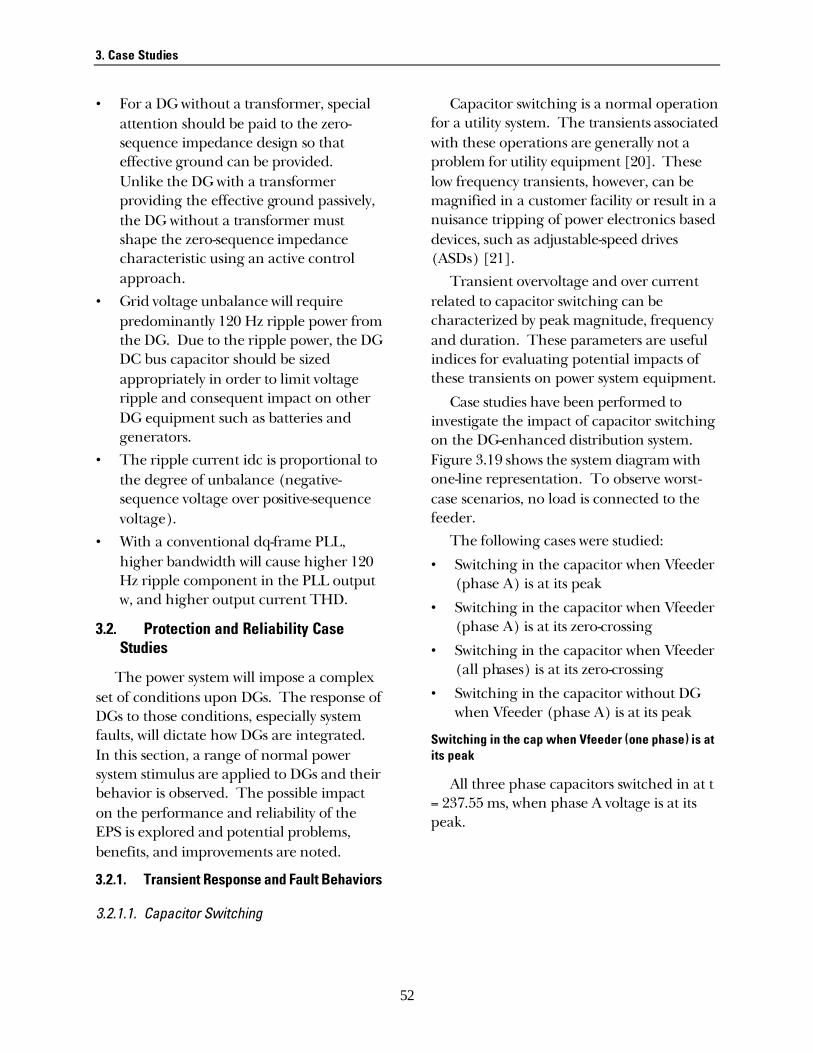
3. Case Studies

52

• For a DG without a transformer, special attention should be paid to the zero-sequence impedance design so that effective ground can be provided. Unlike the DG with a transformer providing the effective ground passively, the DG without a transformer must shape the zero-sequence impedance characteristic using an active control approach.

• Grid voltage unbalance will require predominantly 120 Hz ripple power from the DG. Due to the ripple power, the DG DC bus capacitor should be sized appropriately in order to limit voltage ripple and consequent impact on other DG equipment such as batteries and generators.

• The ripple current idc is proportional to the degree of unbalance (negative-sequence voltage over positive-sequence voltage).

• With a conventional dq-frame PLL, higher bandwidth will cause higher 120 Hz ripple component in the PLL output w, and higher output current THD.

3.2. Protection and Reliability Case Studies

The power system will impose a complex set of conditions upon DGs. The response of DGs to those conditions, especially system faults, will dictate how DGs are integrated. In this section, a range of normal power system stimulus are applied to DGs and their behavior is observed. The possible impact on the performance and reliability of the EPS is explored and potential problems, benefits, and improvements are noted.

3.2.1. Transient Response and Fault Behaviors

3.2.1.1. Capacitor Switching

Capacitor switching is a normal operation for a utility system. The transients associated with these operations are generally not a problem for utility equipment [20]. These low frequency transients, however, can be magnified in a customer facility or result in a nuisance tripping of power electronics based devices, such as adjustable-speed drives (ASDs) [21].

Transient overvoltage and over current related to capacitor switching can be characterized by peak magnitude, frequency and duration. These parameters are useful indices for evaluating potential impacts of these transients on power system equipment.

Case studies have been performed to investigate the impact of capacitor switching on the DG-enhanced distribution system. Figure 3.19 shows the system diagram with one-line representation. To observe worst-case scenarios, no load is connected to the feeder.

The following cases were studied: • Switching in the capacitor when Vfeeder

(phase A) is at its peak • Switching in the capacitor when Vfeeder

(phase A) is at its zero-crossing • Switching in the capacitor when Vfeeder

(all phases) is at its zero-crossing • Switching in the capacitor without DG

when Vfeeder (phase A) is at its peak

Switching in the cap when Vfeeder (one phase) is at its peak

All three phase capacitors switched in at t = 237.55 ms, when phase A voltage is at its peak.

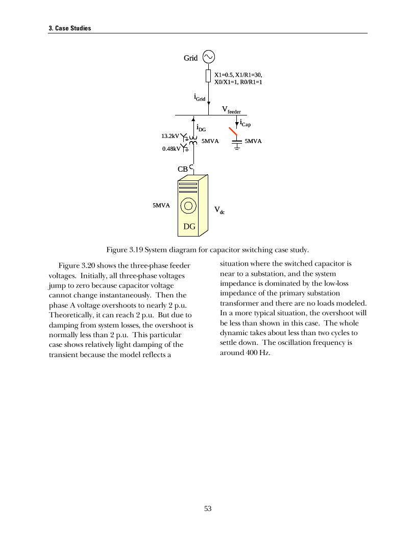
3. Case Studies

53

Grid

CB

13.2kV

0.48kV

DG

Vfeeder

iGrid

iDGiCap

X1=0.5, X1/R1=30,X0/X1=1, R0/R1=1

5MVA

5MVA

5MVA

Vdc

Grid

CB

13.2kV

0.48kV

DG

Vfeeder

iGrid

iDGiCap

X1=0.5, X1/R1=30,X0/X1=1, R0/R1=1

5MVA

5MVA

5MVA

Vdc

Figure 3.19 System diagram for capacitor switching case study.

Figure 3.20 shows the three-phase feeder voltages. Initially, all three-phase voltages jump to zero because capacitor voltage cannot change instantaneously. Then the phase A voltage overshoots to nearly 2 p.u. Theoretically, it can reach 2 p.u. But due to damping from system losses, the overshoot is normally less than 2 p.u. This particular case shows relatively light damping of the transient because the model reflects a

situation where the switched capacitor is near to a substation, and the system impedance is dominated by the low-loss impedance of the primary substation transformer and there are no loads modeled. In a more typical situation, the overshoot will be less than shown in this case. The whole dynamic takes about less than two cycles to settle down. The oscillation frequency is around 400 Hz.

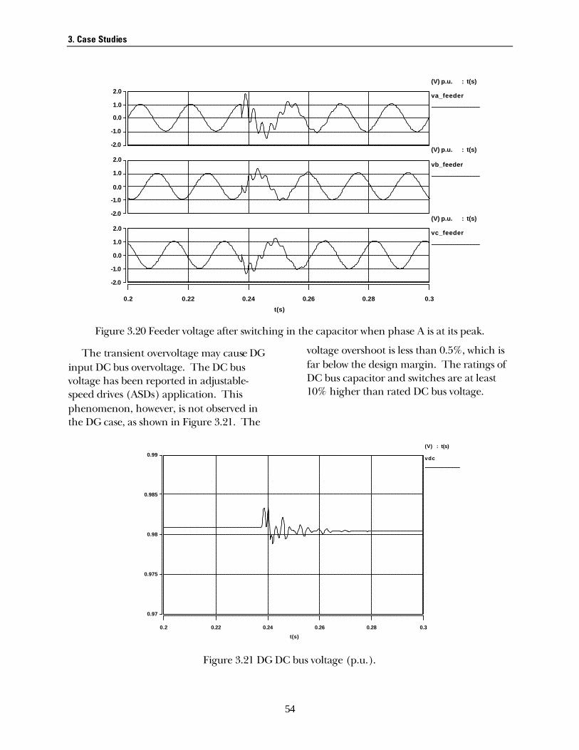
3. Case Studies

54

-2.0

-1.0

0.0

1.0

2.0

t(s)

0.2 0.22 0.24 0.26 0.28 0.3

-2.0

-1.0

0.0

1.0

2.0

-2.0

-1.0

0.0

1.0

2.0

(V) p.u. : t(s)

vc_feeder

(V) p.u. : t(s)

vb_feeder

(V) p.u. : t(s)

va_feeder

Figure 3.20 Feeder voltage after switching in the capacitor when phase A is at its peak.

The transient overvoltage may cause DG input DC bus overvoltage. The DC bus voltage has been reported in adjustable-speed drives (ASDs) application. This phenomenon, however, is not observed in the DG case, as shown in Figure 3.21. The

voltage overshoot is less than 0.5%, which is far below the design margin. The ratings of DC bus capacitor and switches are at least 10% higher than rated DC bus voltage.

0.97

0.975

0.98

0.985

0.99

t(s)

0.2 0.22 0.24 0.26 0.28 0.3

(V) : t(s)

vdc

Figure 3.21 DG DC bus voltage (p.u.).

3. Case Studies

55

The reasons for the different responses between adjustable-speed drives (ASDs) and DG are described below. • For ASDs, the line AC voltages are the

input to ASDs rectifier, typically a diode or thyristor rectifier. The transient overvoltage at the AC side can be directly reflected by the DC side. Therefore, the DC bus overvoltage can be as high as nearly 2 p.u. Due to the fact that the DC bus capacitance will be smaller on an ASD, compared to a PWM DG inverter, the ASD will be more vulnerable to dc-link overvoltage trip.

• For DG, the line AC side is DG’s inverter output. The DG is controlled as a current source to the grid. The grid voltage is the only input for PLL synchronization. Usually, PLL has a low pass filter and its bandwidth is much lower than line frequency. Therefore, the transient overvoltage and high-frequency (in this case, 400 Hz) oscillation will not affect the DG significantly. The PWM inverter simulated in this case uses controls (include current control and PLL) in dq

frame. If the controls are based on zero-crossing in abc frame, then the DG may be more vulnerable to the transient distortion.

Switching in the cap when Vfeeder (one phase) is at its zero-crossing

When the capacitors switch in at phase A voltage zero-crossing, there will be a less severe transient phase A voltage and current. However, the transients in the other two phases are more pronounced, and can also reach nearly 1.8 p.u. overvoltage. There is no significant difference between this case and the previous case.

Switching in the cap when Vfeeder (all phases) is at its zero-crossing

To minimize the transient, a synchronous capacitor switch might be used [22]. Synchronous switching is used more frequently in transmission systems, and is not very common on distribution systems.

The waveforms in Figure 3.22 and Figure 3.23 show significant improvement in the transient behavior.

3. Case Studies

56

-2.0

-1.0

0.0

1.0

2.0

t(s)

0.2 0.22 0.24 0.26 0.28 0.3

-2.0

-1.0

0.0

1.0

2.0

-2.0

-1.0

0.0

1.0

2.0

(V) : t(s)

vc_feeder

(V) : t(s)

vb_feeder

(V) : t(s)

va_feeder

Figure 3.22 Feeder voltage when capacitor switch in at all phases voltage zero-crossing.

0.97

0.975

0.98

0.985

0.99

t(s)

0.2 0.22 0.24 0.26 0.28 0.3

(-) : t(s)

vdc

Figure 3.23 DG DC bus voltage when capacitors switch in at all phases voltage zero-crossing.

3. Case Studies

57

Switching in the cap without DG when Vfeeder (phase A) is at its peak

The event of switching capacitor without DG is also simulated to compare the transients with the case having a DG. Figure 3.24 shows the feeder voltages for both cases. It can be seen that the DG adds additional damping to the transient. Typically, the DG has nearly infinite impedance at 60 Hz due

to its current regulation. However, the transient frequency (400 Hz in this case) is not within DG’s current regulation bandwidth. Therefore, the DG has a finite impedance at the transient frequency which provides some beneficial damping effect. This damping is likely to be much less significant than the damping provided by loads.

t(s)

0.2 0.22 0.24 0.26 0.28 0.3

-2.0

0.0

2.0

-2.0

0.0

2.0

-2.0

0.0

2.0

(V) : t(s)

vc_feeder

vc_feeder

(V) : t(s)

vb_feeder

vb_feeder

(V) : t(s)

va_feeder

va_feeder

Figure 3.24 Transient dynamics with (solid line) and without DG (dotted line).

Conclusions

• Energizing a shunt capacitor bank from a predominantly inductive source can result in an oscillatory transient that can ideally approach twice the normal system voltage. The problem can be minimized by synchronous control of the capacitors. Synchronous closing, however is only occasionally applied on high-voltage transmission systems, and not a common practice in distribution systems.

• Because capacitor voltage cannot change instantaneously, energization of a capacitor bank results in an immediate

drop in system voltage toward zero, followed by an oscillating transient voltage superimposed on the 60Hz fundamental waveform. The peak voltage magnitude depends on the instantaneous system voltage at the instant of energization, and can reach two times of the normal system voltage under worst-case conditions. The transient frequencies generally fall in the range of 300–1000 Hz, depending on the inductance of the system and capacitor bank ratings.

• Transient overvoltage due to capacitor switching is generally just below the level

3. Case Studies

58

at which utility distribution system surge protection, such as arresters, begin to operate. However, these transients will often be coupled through step-down transformers to customer equipment. While the impact of the transient on some load, such as ASDs, is significant, its impact on DG can be minimal due to the nature of the DG control and operation.

• While the switching capacitor has little impact on DGs dynamics, one noticeable benefit of DG during capacitor switching is that DG adds additional damping to the transient. The dynamics of the event with DG is noticeably improved comparing with those without DG.

3.2.1.2. Fault Analysis

The impact of DG units on fault currents can be significant. This can affect the reliability and safety of the distribution system. The fault behavior of rotating generators is well known and well documented [23]. Newer DG technologies will predominantly be of the power electronic variety. Hence, this study focuses the behavior of power electronic DGs during fault in the utility system.

The DG considered for this study is a 3-phase 4-wire with a delta-wye transformer at the DG output. The DG inverter is current controlled to inject the required real and reactive power into the grid. It is normally controlled as unity power factor, thus the reactive power reference is zero.

The fault contribution from a single small DG unit is not large, however, the aggregate contributions of many small units, or a few large units, can alter the short circuit levels enough to cause overcurrent protection (fuse-breaker) miscoordination, excessive fault currents, nuisance fuse operation, and

hamper fault detection. For example, normally it will take five to six cycles for the upstream breaker using an instantaneous trip setting to clear a fault, hence a fuse needs to be sized so that its minimum melt time is longer than the total breaker fault clearing time (must be at least six cycles plus some margin time). If the fault current increases due to DG contribution to the fault current, its minimal melt time may be significantly shorter than six cycles and it will no longer coordinate with the circuit breaker. The coordination of the fuse and the time overcurrent relay at different fault current level is critical to power system protection. It is possible for the DG to maintain voltage on a distribution feeder and reduce the fault current level at the substation. This can further delay the operation of the time overcurrent relay. Some utilities have a policy where they would prefer a down stream fuse to open and thus prevent disruption on the rest of the distribution feeder. This study is focused on the fuse saving strategy previously discussed. However, fault current contributions of the inverter-DG under different conditions are studied and compared to those of an induction motor load.

Figure 3.25 shows the system under study with one-line diagram. The following cases were studied: • Three-phase ground fault with DG • Single-phase ground fault with DG • Three-phase ground fault with DG and

feeder fault (X1=0) • Three-phase ground fault with induction

machine The system with both high source

impedance and low source impedance is studied.

3. Case Studies

59

CB

13.2kV

0.48kV

DG

Grid

Source impedance

Vfeeder

iGrid

iDG iFault

X1=0.5, X1/R1=30,X0/X1=1, R0/R1=1

5MVA

5MVAFeeder

X1=1, X1/R1=3,X0/X1=3, R0/R1=4

CB

13.2kV

0.48kV

DG

Grid

Source impedance

Vfeeder

iGrid

iDG iFault

X1=0.5, X1/R1=30,X0/X1=1, R0/R1=1

5MVA

5MVAFeeder

X1=1, X1/R1=3,X0/X1=3, R0/R1=4

Figure 3.25 One-line diagram of the system under study.

Three-phase to ground fault with DG

The fault occurs at the remote end of the feeder. The fault lasts for 0.2 s and is then cleared. Figure 3.26 shows the fault, grid

and DG currents. Since the DG is current controlled, it will supply constant current with a short transient when the fault occurs and clears. It can be seen that the grid supplies the majority of the fault current.

3. Case Studies

60

Figure 3.26 Feeder 2, grid and DG high side phase A current during fault.

During the fault, the feeder voltage will drop. The voltage drop is dependent on the fault impedance and the line impedance to the point of fault occurrence, which is proportional to the distance of the fault. In this case, the voltage drop is not large or long enough to trip the DG. The DG under/overvoltage trip settings are based on

P1547 requirements. Figure 3.27 shows per-cycle I2t of the fault, grid and DG currents. The per-cycle I2t is calculated every period of the fundamental output current. The per-cycle I2t value provides information on the coordination of the fuse and time-overcurrent relay in the system.

Figure 3.27 Cycle-by-cycle I2t contribution from feeder2, grid and the DG.

3. Case Studies

61

In this case, the DG fault current contribution is only a very small fraction of the total fault current. Therefore, it is not likely to affect fuse-breaker coordination. It has also been studied that the DG fault current contribution has a larger percentage with higher DG penetration and under weaker line conditions.

Single-phase to ground fault with DG

Figure 3.28 shows the fault, grid and DG currents during a single-phase fault. It is

found that the DG current contribution to the fault is slightly larger than that due to the three-phase fault. This is due to the DG delta-wye transformer, which provides a path for zero-sequence current. The zero-sequence currents of DG, grid, and fault are shown in Figure 3.29. The magnitude of the zero-sequence currents depends on the X0 to X1 ratio.

Figure 3.28 Feeder2, grid and the DG high side current on the faulted phase.

3. Case Studies

62

Figure 3.29 Zero sequence currents of fault location, grid and DG.

Similarly, during the single-phase fault, the I2t contribution of the grid and the fault are almost identical. The I2t of the DG is miniscule by comparison.

As a conclusion, under both three-phase and single-phase fault, the inverter-based current controlled DG has little impact on fault contribution and fuse-saving strategy.

Three-phase to ground fault at the feeder (X1=0)

When the fault is right at the feeder (X1=0 for the feeder in Figure 1) where the DG is connected, the DG will trip due to undervoltage. The tripping time for voltage under 50% is user defined but the maximum

is 0.16 s as required in P1547. This maximum limit is to ensure that the DGs are offline before any recloser action. Disconnecting the DGs too fast can reduce the benefits to the power system provided by the DG during faults, as described in the “Power systems dynamics and stability” case study section.

Figure 3.30 shows the per-cycle I2t contribution at the fault, grid and DG. Again, the fault current contribution is predominantly from the grid. The DG's current contribution, which is already small, is further reduced when the DG trips off-line.

3. Case Studies

63

Figure 3.30 Cycle-by-cycle I2t contribution during fault at the feeder, grid and the DG.

Three-phase to ground fault with induction machine

Utilities have experience evaluating the impact of motor loads on the distribution feeder fault current. Hence, a study was carried out to compare the DG with an induction machine load at the same power level. The machine considered in the case study is an aggregate of many small machines. The parameters of the individual machine are listed in Table 3.3. The machines are connected in a three-phase three-wire configuration. The machine models include both stator and rotor flux dynamics. Magnetic saturation is not captured in the simulation. The modeled mechanical load has a quadratic speed-

torque relationship. Figure 3.31 shows the one-line diagram of the system under study.

Table 3.3 Parameters of the induction machine

Vll_rated 480V

Power 15hp

Rs 0.0301pu

Rr 0.0064pu

Xm 2.3120pu

Xls 0.0665pu

Xlr 0.0116pu

Jpu 2.6672s

Dpu 0.0197pu

3. Case Studies

64

13.2kV

0.48kV

Grid

Source impedance

Vfeeder

iGrid

iFault

X1=0.5, X1/R1=30,X0/X1=1, R0/R1=1

5MVAFeeder

X1=1, X1/R1=3,X0/X1=3, R0/R1=4

iMotor_h

IM

5MVA

13.2kV

0.48kV

Grid

Source impedance

Vfeeder

iGrid

iFault

X1=0.5, X1/R1=30,X0/X1=1, R0/R1=1

5MVAFeeder

X1=1, X1/R1=3,X0/X1=3, R0/R1=4

iMotor_h

IMIM

5MVA

Figure 3.31 One-line diagram of the system for fault studies with induction machine load.

Figure 3.32 shows the fault, grid and motor (transformer high side) currents. It can be observed that the motor phase current has a phase jump at the beginning of the fault, signifying that the motor momentarily feeds power into the grid. There is an initial drop in the current magnitude because of the drop in the voltage magnitude. However, it can be observed in Figure 3.33 that the per-cycle I2t

increases as the fault proceeds because of the increased motor slip, caused by the sag in the motor terminal voltage. Once the fault is cleared, the terminal voltage increases leading to an inrush into the induction machine. Figure 3.34 shows the motor torque and speed response to the fault. It is clearly seen that the fault current contribution from motor is larger than inverter-DG.

3. Case Studies

65

Figure 3.32 Currents in feeder, grid and motor transformer high side during the fault event.

Figure 3.33 Cycle-by-cycle I2t contribution in the feeder, grid and induction motor high side during the fault.

3. Case Studies

66

Figure 3.34 Machine torque and speed during the fault.

3.2.1.3. Summary

The I2t contributions of the DG and the grid into the fault are summarized in Table

3.4 for the various cases studied. These values represent the contribution during the fault condition in the system.

Table 3.4 Comparison of the I2t* contribution during the different fault cases

Fault Grid DG/IM

With DG & low source impedance 5.13Meg 4.99Meg 3348

Without DG & low source impedance 5.1Meg 5.1Meg 0

With Induction Machine 5.04Meg 5.3Meg 15873

With DG & high source and fault impedance 407 277.5 35.85

Without DG & with high source and fault impedance 377 377 0

Single phase to ground fault 2.35Meg 2.14Meg 7246

* I2t has been calculated over 200ms fault duration.

As can be noted from the above table, for the case with the low source impedance, the contribution of the DG is negligible. However, for the case of a high impedance fault, where the grid connection is through a weak line (highlighted rows), there is a significant reduction in the I2t contribution

by the grid with the DG present in the system. This is an extreme case, however, and does not imply that the DG would be the cause of fuse mis-coordination. The fault current is too small in this case, with or without the DG, to operate a grid-side fuse, which has been sized to accommodate a load comparable to the DG rating.

3. Case Studies

67

3.2.1.4. Conclusions

• Current output from the inverter-DG remains at the load current setpoint, except for a minor and brief transient.

• For inverters, the fault contributions will depend on its operating current level and the DG under voltage protection trip settings.

• In a current-controlled inverter DG, the single-phase fault will cause zero-sequence current in a four-wire system. Because of the zero-sequence current, the faulted phase DG current is larger than the one with balanced three-phase fault.

• For induction motors, the significant current lasts only a few cycles and is determined by dividing the pre-fault voltage by the transient reactance of the machine. The fault current contribution is usually much larger than that of current controlled inverter-DG. It is common practice to ignore the fault current contribution of induction motor loads, particularly small, distributed motor loads, in distribution overcurrent conditions. The results show the DG is much smaller than that of the motor loads. Thus, there is ample precedent for considering current-controlled inverter-based DG as an insignificant short circuit current condition. However, the fault impact of DGs needs to be reevaluated in case the DG controls are changed to accomplish other functions such as voltage support.

• I2t contributions for weak system might be concern with increased DG penetration.

• Modern inverter-based DGs do not contribute to system fault current beyond the pre-fault operating current level. However, the current contribution of the

DG system to a single phase fault may be greater than the three phase case which conflicts with IEEE P1547 (Draft 07) requirement that ground fault current contribution of a DG shall not be greater than 100% of the fault current contribution of the DG to a three phase fault. This is because the DG is a nearly ideal current source for the positive sequence, but is generally a constant impedance or voltage source for the zero sequence. Both are desirable characteristics, and the result reveals that the wording of P1547’s single-phase to three-phase fault current ratio requirement is more appropriate for conventional rotating generators. The wording of this requirement needs additional consideration with respect to its consistency with inverter-based applications.

3.2.2. Anti-Islanding Protection of DG

Islanding of a grid connected DG occurs when a section of the utility system containing such generators is disconnected from the main utility, but the independent DGs continue to energize the utility lines in the isolated section (termed as an island). Unintended islanding is a concern primarily because it poses a hazard to utility and customer equipment, maintenance personnel and the general public. Poor power quality can damage loads in the island. Another concern is the out of phase switching of the recloser leading to damage to the DG, neighboring loads and utility equipment. Any feature available to reduce the run-on time of an islanded system can be termed as “anti-islanding.”

Many techniques have been proposed to prevent islanding caused by DGs [25-46]. An algorithm proposed by the Sandia National Laboratories is analyzed in this study because

3. Case Studies

68

it is considered to be effective. Sandia’s active islanding algorithms had been developed for single-phase inverter units. The algorithm consists of the Sandia frequency shift (SFS) and the Sandia voltage shift (SVS) schemes. The principle behind both the methods is an accelerated frequency and voltage drift respectively created with positive feedback. In the presence of the utility, the frequency and voltage shifts are not effective in drifting the two parameters. However, once the grid is disconnected, these methods force the frequency and/or voltage to shift outside the operating windows, causing the inverter to disconnect due to o/u voltage and frequency protection.

Since these were originally developed for a single phase inverter, the technique adopted to measure frequency is based on the zero crossing of the voltage waveform, and the voltage magnitude is obtained from RMS calculations. This method has been extended to three phase DGs by GE and has been studied under the NREL contract.

3.2.2.1. Analysis of Sandia Anti-Islanding Algorithm

A block diagram representation of the Sandia’s algorithm is shown in Figure 3.35.

The first step is to determine the gain settings for the Sandia voltage scheme (SVS) and the Sandia frequency scheme (SFS) algorithms. The critical gains of the Sandia anti-islanding algorithm are: • Kf for the SFS • Kvp and Kv for SVS • wf1 for the wash out functions • wf2 for the power regulation loop

The critical gains for SFS and SVS have to be determined for RLC loads (set according to IEEE P1547) so as to mitigate islanding situations. The gain settings of the algorithm, shown in Figure 35, have been obtained by performing a small signal analysis of the DG system with the tuned RLC load (according to IEEE 929 2 and IEEE P1547 anti-islanding test specifications).

The algorithm gains are determined by investigating the open loop behavior as a function of frequency. The voltage magnitude and the phase signal flow paths were opened so as to obtain the SVS and SFS gains, respectively. The Sandia voltage and frequency schemes are explained in detail below.

3. Case Studies

69

P%

dr

nr

∆ ω

θV

|V|

ω̂

Anti-islanding algorithm

P*Kvp+Kv

Kf

s/ωf1

1 + s/ω f1

s/ωf1

1 + s/ω f1

∆P

11 + s/ω f2

Inverter

P*

Q*

%dr

nr

Iq*

∆ θ*

(I,θ i)

(V,θv)

Grid/Load(ωg)

1/s

tan-1(Iq*/Id*)

Iq*2 + Id*2

Id*

GP

SA

Rθ2ωg

+

+

+

+

I

θ i

ZCD PLL

+

θ̂

φ

Figure 3.35 The block diagram representation of the Sandia’s anti-islanding algorithm.

Sandia’s frequency shift (SFS) algorithm

The block diagram of the SFS algorithmis shown in Figure 3.36. The frequencyestimate from the phase lock loop is passedthrough a washout function to determinechanges in the ambient frequency. Thisinformation multiplied by the SFS gain, isadded to the frequency reference of thecurrent injected by the DG inverter. As theDG commanded frequency on averagecannot be different from the grid frequency,the phase angle has to be periodically resetfor meaningful power transfer from the DGto the rest of the grid system to occur. In thesingle phase case, this reset of the phaseangle in the DG current reference waveformoccurs at the voltage zero crossings.

In the SFS modification for a three-phaseDG, the frequency of the system isdetermined using a continuous trackingPhase Locked Loop (PLL) in a synchronousreference frame. This frequency estimate isthen passed through a washout, todetermine the trend in system frequency.The change in estimated system frequency ismultiplied by the SFS gain constant (Kf) to

obtain the increment or decrement in theoutput frequency of the DG inverter'scurrent injection into the grid.

The Rθ/2wg block in Figure 3.36 is anequivalent representation of the actual DGsystem behavior that captures the change inthe phase corresponding to the error infrequency. The derivation of this block inthe grid parallel mode (GP) is based on theequivalent phase angle change (φ)calculated in response to a change infrequency (∆w) as a function of the systemfrequency (wg). This can be explained byconsidering the single-phaseimplementation where the frequencycommand from the SFS is higher than thenominal frequency and reset period of 180o,as shown in Figure 3.37.

θπωθ

RT

/2⋅∆=∆

,

where, T is the period and Rθ is the resetangle. Simplifying for the period in terms ofw, we get

g

Tωωθ ⋅∆=∆

.

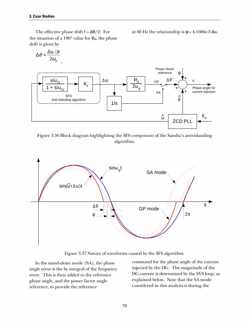
3. Case Studies

70

The effective phase shift f = ∆θ/2. Forthe situation of a 180° value for Rθ, the phaseshift is given by

gωπωθ

2⋅∆=∆

,

at 60 Hz the relationship is φ = 4.1666e-3 ∆w.

∆ ω

θVω̂

SFSAnti-islanding algorithm

Kfs/ω f1

1 + s/ω f1

∆ θ*

1/s

GP

SA

Rθ2ωg

+

+θ i

ZCD PLL

+

θ̂

φPower factor

reference

Phase angle forcurrent injection

Figure 3.36 Block diagram highlighting the SFS component of the Sandia’s anti-islandingalgorithm.

θ

sinωgt

sin(ω +∆ ω )t

∆ θ

2πφGP mode

SA mode

Figure 3.37 Nature of waveforms caused by the SFS algorithm.

In the stand-alone mode (SA), the phaseangle error is the by integral of the frequencyerror. This is then added to the referencephase angle, and the power factor anglereference, to provide the reference

command for the phase angle of the currentinjected by the DG. The magnitude of theDG current is determined by the SVS loop, asexplained below. Note that the SA modeconsidered in this analysis is during the

3. Case Studies

71

transition of from grid parallel mode. In thiscondition the grid has been disconnectedbut the DG has not yet made any decisionfor mode transition and continues to injectcurrent out of its terminals.

Sandia’s voltage shift (SVS) algorithm:

The block diagram of the SVS algorithmis shown in Figure 3.38. The input to thisblock is the magnitude of the system voltage.The error in the system voltage determinesthe shift in the reference power, to drive the

DG voltage further away from the operatingvoltage range. The voltage magnitude, aftera low pass filter, is also used to determine themagnitude of the reference current settingsfor the DG. This is to ensure that thedesired level of real and reactive power isbeing delivered by the DG. As compared tothe SFS, the gain in the feedback loop is nota constant, but is a function of the real powerreference setting. This is to reduce thedependence of the SVS algorithm on thereference power setting.

P%

dr

nr

|V|

SVSAnti-islanding algorithm

P*Kvp+Kvs/ω f1

1 + s/ω f1

∆P

11 + s/ω f2 P*

Q*

%dr

nr

Iq*

Iq*2 + Id*2

Id*+

+

I

Magnitude ofoutput voltage

Magnitude forcurrent injection

Figure 3.38 Block diagram highlighting the SVS component of the Sandia’s anti-islandingalgorithm.

The anti-islanding algorithm works byforcing the island with the DG to becomeunstable whenever the grid is disconnected.Hence, for the active anti-islanding to beeffective, the open loop gain has to begreater than one. Once the SFS and SVSgains are obtained, the time domainsimulations for RLC and motor loads areconsidered in order to verify the behavior ofthe algorithm using detailed three-phaseload and DG models. The next sectioninterprets the characteristics of the SFS andSVS active anti-islanding algorithms basedon frequency domain analysis.

3.2.2.2. Implications of the Gains Settings of theSandia Anti-Islanding Algorithm

One of the goals of the analysis of blockdiagram representation of the anti-islandingalgorithm is to evaluate the dependence ofthe gain settings of the SFS and SVS on thetype of load. Passive and active loads areconsidered. The gains should be designedfor the worst-case load for the schemes to beeffective under all circumstances. R andRLC loads are evaluated for passive loading.High and low inertia three phase inductionmachines loads are evaluated for activeloads. Driving induction machine loads withcurrent source DG, without explicit speedcontrol loops, are not feasible on a sustainedbasis. This makes the task of evaluating theanti-islanding algorithm with inductionmotor loads, at different DG and load

3. Case Studies

72

parameters, a challenging task using timedomain small signal techniques. Hence thistask is deferred to the section on timedomain analysis. Therefore all thediscussion below is for RLC loads with the Land C set so that the load has a quality factorof 2.5 as defined in IEEE 929 and IEEEP1547 testing requirements. For the purposeof analysis, the SFS and SVS loops areconsidered decoupled except at the load.The voltage magnitude fed back into SVS isheld at the nominal value during the studyof SFS algorithms. The frequencymeasurement into SFS is held at the nominalvalue (60 Hz) during the analysis of the SVSalgorithm.

Figure 3.39 shows the open loop gainfrequency response of the SFS algorithm

with the RLC load at 50% and 100% powerlevel. The gains are the open loop gainsobtained by breaking the θv signal flow pathin Figure 3.35. All gains referred to in theanalysis are calculated in per unit on the DGbase. It can be seen the response is nearlyflat for low frequencies (10 Hz and below)and droops down at higher frequencies.Gains greater than 0 dB are inherentlyunstable because it results in positivefeedback under closed loop conditions withphase angle approximately zero (not shownin the plot). It can be observed that the loadpower levels did not affect the loop gain ofthe SFS algorithm. This implies that thepower level of DG operation does not affectthe SFS.

Figure 3.39 Loop gain of the SFS algorithm with RLC load at 50% and 100% power level.

Similarly, Figure 3.40 shows the openloop gain frequency response of SVSalgorithm. In this case the loop gains areobtained by opening the |V| signal flow pathshown in GE's interpretation of the blockdiagram representation of the Sandia’s anti-

islanding algorithm. The loop gaincharacteristics of the SVS algorithm is flat atlow frequencies (below 5 Hz). Themagnitude of the gain is higher than 0dBindicating that the SVS algorithm will be

3. Case Studies

73

effective (i.e. unstable) for the gains shown in Figure 3.40.

Figure 3.40 Loop gain of the SVS algorithm for varying Kvp, with Kv = 1, for RLC loads.

Figure 3.41 indicates additional characteristics of the SVS loop gain, as a function of the gain constants Kv and Kvp. It can be observed that the SVS loop gain characteristics have a tendency to reduce as load is increased. At light loads, it can be observed that there is lower sensitivity of the SVS loop gain to variations in kvp (keeping kv = 1). It can be observed from Figure 3.41 that at overloads the SVS loop has lower sensitivity to kv (keeping Kvp = 1). In

general it was observed for all loads, there is a cross over of the dominant gain from Kvp to Kv at the value of 1. At full load, the loop gain follows the same path for variations in either Kv or Kvp. This can be explained by the fact that at rated load, the equivalent gain offered by the algorithm is just the sum of Kv and the product of Kvp and Power. At 100% power the gain in each of these paths equals unity.

3. Case Studies

74

Figure 3.41 Varia tions of loop gain in dB at 2 Hz for varying load power level and gain constants of the SVS (keeping the other parameters fixed).

The plots on Figure 3.42 are obtained by keeping one gain (either Kp or Kvp) constant at 1pu and varying the other gain at different output power levels. Figure 3.42 (a) and (b) indicate that as the loading on the DG increases, the loop gain has a decreasing trend. This means that the SVS algorithm tends to be less effective for higher loadings. This is because a portion of the SVS response is independent of the operating power level. At high loadings, the system is less sensitive, meaning the voltage change per Watt of DG output power change is less. Ideally, the gains should have remained constant even for any change in power output.

Figure 3.42(c) shows the effect of increasing Kvp at different load levels. The curves at different power levels tend to converge as the gain is increased. Figure 3.42(d) shows the effect of increasing Kv at

different load levels. The curves at different power levels tend to diverge as the gain is increased. Hence, an optimum tradeoff between Kv and Kvp has to be obtained that minimizes the sensitivity of SVS to load power level. The term Kvp, which multiplied by Power, tries to make it more insensitive to load power level when compared to using a single gain constant in the feedback path of the SVS as described in the explanation for Figure 3.41.

Figure 3.42 (c) and (d) indicate that higher the gain the higher the instability causing faster detection of an islanding situation. However, setting the gains too high leads to greater harmonic distortion in the DG load current. Hence, a minimum acceptable gain has to be selected.

3. Case Studies

75

Figure 3.42 Influence of load and gain constants on the SVS loop gain. (a) effect of load (%) on the loop gain (dB) at various Kvp (p.u.); (b) effect of load (%) on the loop gain (dB) at various Kv (p.u.); (c) effect of Kvp gain (p.u.) on loop gain (dB) at various loads (%); (d) effect of Kv

gain (p.u.) on loop gain (dB) at various loads (%).

Washout and power regulation time constants

The schemes use a number of parameters (wf1, wf2, Kvp, Kv, Kf) that have to be set appropriately for the algorithm to operate properly. The corner frequency wf1 is set to differentiate between a change in measured frequency or voltage due to variation in DG’s operating point and other slow dynamics of the power system. Hence, wf1 is set to 0.1 Hz. Hence, voltage or frequency changes that occur in a time of less that 10s can excite the anti-islanding algorithm. If the voltage or frequency change sustains for longer than 10 s then it is considered a change in the

nominal operating condition. The corner frequency w f2 is set to 0.01 Hz. This is used to filter the measured voltage amplitude, which is then used to obtain the current command from the power command. In case the DG terminal voltage rises, the anti-islanding algorithm tries to increase the power command, while the power regulation loop through wf2 lowers the reference current magnitude to maintain constant real and reactive power level. The corner frequency of wf2 has been set to be decade lower than wf1 in the anti-islanding algorithm, so that the change in current magnitude due to voltage regulation and

3. Case Studies

76

anti-islanding do not counteract each other. The setting of 0.01 Hz corner frequency will also allow the DG prime mover to respond and change its power level in a time frame (of the order of 10 s) to a change in the measured output voltage.

The range of values for the SFS and SVS gain determined from the above analysis provides design space for time domain simulations of the DG system. The time domain simulations are application dependent and need to be considered on an individual basis. The time domain simulations will provide acceptance trade off curves between the time to detect island and harmonic distortion.

3.2.2.3. Time-Domain Simulations

Detailed time domain simulations of the system have been carried out with passive and active loads using the SVS and SFS algorithm described in the previous sections. The circuit considered for the time domain simulation is shown in Figure 3.43. The following cases are described below:

• RLC load without anti-islanding algorithm

• RLC load with anti-Islanding algorithm • Motor load having high inertia • Motor load with low inertia.

The gains of the SFS and SVS algorithms were selected to be within the range obtained from the analysis in the previous sections. However, a detailed trade-off study has not been performed to pick optimum gains. The gains for all the above cases studied are the same— • Gain setting for SFS is 10 • Gain setting for SVS is Kv = 2 and Kvp =

2—i.e., a sum of four for the case with DG supplying rated load at unity power factor.

• The DG power level is 5 MW and it injects current into the grid at unity power factor.

Figure 3.43 Single line diagram for testing the anti-islanding scenario.

3. Case Studies

77

RLC load without anti-islanding algorithm

The RLC resonant load was first tested without any anti-islanding protection. The waveforms for this case are shown in Figure 3.44. It can be observed from the voltage and current waveforms, that the DG continues to feed the RLC load and forms an island. The frequency and voltage drift by a small amount due to a minor difference in

RLC values and due to the small numerical mismatch between the real and reactive power in the load and generator. However, the drifts in frequency and voltage magnitude are not sufficient to detect an islanding situation in an acceptable time frame (based on the passive anti-islanding limits on voltage and frequency set according to IEEE P1547).

(a)

(b)

Figure 3.44 Waveforms for the RLC load without anti-islanding protection (a) load phase voltage, (b) current.

3. Case Studies

78

RLC load with anti-islanding algorithm

Figure 3.45 depicts the voltage and current at the DG terminals for the RLC load, for the case where the active anti-islanding algorithm is enabled. The system

was islanded at time 0.70037 s by disconnecting the grid. The DG detected the island and tripped due to a drift in the frequency because of the active anti-islanding algorithm.

(a)

(b)

Figure 3.45 Waveforms for RLC load with Kf = 10 and Kv and Kvp = 2 (a) load phase voltage and (b) current waveforms.

Motor load with high inertia and anti-islanding algorithm

The next load considered is a three phase induction motor load with a high inertia (J(pu) = 2.6s). The motor operates such

3. Case Studies

79

that the entire 5MW generated by the DG is consumed by it. The reactive power consumed by the machine is fully compensated by capacitor banks at the 13.2 kV bus (Figure 3.43). The settings for the algorithm are the same as for the other cases. Figure 3.46 shows that the DG has a tendency to drift on. The trip is finally detected at around 1.92 s.

For the purpose of specifying anti-islanding performance, IEEE 929 characterizes the islanded power system by a “Q factor”. For a simple R-L-C passive load, the Q-factor accurately characterizes the tendency of the resonant 60 Hz circuit to run on at a constant frequency and voltage magnitude. With motors in the system, however, the Q factor definition is ambiguous. Commonly, the Q factor is determined assuming the motor load as a parallel or series R-L circuit, which when rated voltage and frequency are applied, produces a real and reactive load flow

equivalent to the actual motor. Note that motor inertia is not used to define the circuit Q factor in this approach, yet the case results clearly illustrate the importance of this parameter. This implies that the Q factor approach, as typically applied, is not a valid measure of anti-islanding scheme performance when motors are present in the islanded load. It should be noted that motors usually constitute a large portion of a typical system load.

Motor load with low inertia

For the case shown in Figure 3.47, the motor inertia is 0.4 s (p.u.) with all other parameters remaining the same. The DG, which acts as a current source, accelerates the motor after being disconnected from the grid. As a result, the anti-islanding algorithm detects the frequency drift beyond the limit points and trips. The trip time in this case is reduced to 0.328 s.

3. Case Studies

80

(a)

(b)

Figure 3.46 Waveforms for islanding situation with a high inertia motor. (a) load phase voltage, (b) current waveforms.

3. Case Studies

81

(a)

(b)

Figure 3.47 Waveforms when the island load is a low inertia motor. (a) load terminal voltage, (b) currents.

3.2.2.4. Summary

• The DG without active anti-islanding has a tendency to island for a resonant RLC

load, thus creating a number of possible hazardous conditions for the system.

• The single-phase Sandia’s anti-islanding algorithm can be effectively adapted for

3. Case Studies

82

three phase DG applications. In frequency domain it has been observed that the loop gains did not vary with the load type. The algorithm when tuned for rated DG power level will be effective under all realistic operating conditions.

• The algorithm is not as effective for some induction motor loads. In particular, it is not very effective for large inertia loads with significant reactive compensation. More research is needed to fully quantify these loads and to investigate anti-islanding alternatives.

• A tuned RLC circuit does not adequately represent the islanding behavior of circuits containing significant amount of induction motor load. A circuit with motors cannot be adequately characterized by a Q factor based on real power load, reactive load, and capacitive compensation. Motor inertia has a large effect on islanding performance, yet this parameter is not reflected at all by the conventional Q definition.

3.2.3. Reclosing

Reclosing of breakers after a temporary fault is a common practice to prevent extended interruption of supply to end customers. The fault clearing breakers are delayed from closing after a fault to allow the fault path to deionize [24]. The time delay provided for reclosing is generally

determined by the nature of the load, which the recloser is protecting.

3.2.3.1. Out of Phase Reclosing

The introduction of DG adds to the complexity of the issue. Normally, with anti-islanding protection, the DG will trip off-line when grid is disconnected. However, the possibility of DG run-on always exists. If the DG continues to feed an island with motor loads and capacitive components, a situation may arise wherein the recloser closes onto an island when the grid and DG voltage are not in phase, or out of phase in worst case. The out-of-phase reclosing will cause overvoltage and large inrush current, which may damage equipment in the system. Appropriate relays required to prevent such an occurrence are rarely installed along with distribution reclosers. This section will illustrate the effects of out of phase reclosing on the distribution network.

The circuit considered for this case study is shown in Figure 3.48. For a typical distribution network, induction motors comprise a large percentage of the total load. Capacitors are also commonly present in the system for voltage regulation or power factor correction. Cables and lines will also contribute stray capacitance to the system.

3. Case Studies

83

Figure 3.48 One line diagram of the circuit used to study impact of reclosing.

The DG is controlled to supply rated power at unity power factor. The capacitors on the 13.2 kV bus provide voltage support by compensating the reactive power needed by the motor. The capacitor provides about 1.3 MVar ensures that there is no reactive power miss-match when the recloser opens.

If the DG runs on when the grid is disconnected, a small frequency difference can lead to a large phase angle difference between the DG and the grid. Given a typical recloser delay time setting and islanded DG frequency, the phase shift of the grid and DG may not always be very large by the time of reclosing. However, to evaluate the worst-case conditions, this study will look at reclosing with nearly 180° out-of-phase conditions.

To illustrate the impact on the presence of DG on reclosing, the following scenarios are studied: • Three-phase reclose with motor load of

high inertia with DG.

• Three-phase reclose with motor load of high inertia without DG.

• Three-phase reclose with motor load of low inertia with DG.

• Three-phase reclose with motor load of low inertia without DG.

Three-Phase reclosing with high-inertia Motor Load and with DG

The recloser disconnects the DG from the grid and the DG continues to supply the island with the motor load and the capacitor. The voltage of the island drifts out of phase from that of the grid due to a slight unbalance in the loads and also due to the active anti-islanding algorithm can lead to frequency shifts. The recloser is closed when the grid and DG are 180º out of phase in phase A, at around 0.763 s, as shown in the Figure 3.49. This results in the characteristic ringing in the voltage, with overvoltages more than 2 p.u. This voltage magnitude may be sufficient to damage

3. Case Studies

84

utility and customer equipment, including surge arrestors.

Figure 3.49 Phase voltage waveforms of the DG and grid showing the effect of out-of-phase reclosing.

Due to the reclose, nearly twice the rated volt-second is applied to the motor terminals resulting in a heavy inrush current in the motor. Magnetic saturation characteristic, which is not represented in the simulation, can lead to even larger inrush current. This

current is supplied by the grid, since the DG is controlled as a current source with current limit. The currents supplied by the DG, grid, and that drawn by the load are shown in Figure 3.50.

Figure 3.50 Inrush currents observed for the motor load after the three phase reclosing.

3. Case Studies

85

Three-Phase reclosing with large inertia motor load and without DG

As a comparison, the reclosing was simulated for a system with the grid supplying the motor and capacitor load only without DG. A 180° phase shift is set before reclosing for consistent comparison. In this case, it is assumed that the large inertia and flux in the machine along with the capacitive compensation sustains the voltage of the load system. The waveforms obtained are shown in Figure 3.51.

The results indicate that any element in the power system that can store sufficient energy and if it can sustain an island can lead to out of phase reclosing. In practice, however, motors alone without DG will not

usually sustain an island for the typical distribution reclose times, as there is no source of real power other than the rotational energy stored in the inertia.

If, in some unusually circumstance, motor inertia alone sustains a system until reclosing, the resulting out of phase reclosing transients may be more severe than might occur for an island sustained by a DG. The oscillations observed in the case without the DG have a larger magnitude and last for a longer time as compared to the case with the DG. This indicated that the DG, in this example, provides some damping to high frequency oscillations.

Figure 3.51 Voltage waveforms for the reclosure action when the DG is absent.

Three-phase reclosing with low-inertia motor load and with DG

It is common for most machine loads in an ordinary distribution feeder to have lower inertia. Hence, the impact of the reclosing

on an island with a low-inertia (0.4 s) motor is studied both with and without DG.

Typical waveforms observed are shown in Figure 3.52. The reclosing is carried out 0.3 s after the trip. If the reclosing time is further increased, the DG will trip because of

3. Case Studies

86

undervoltage. The capacitive compensation and the power injected by the DG is such that the real and reactive power drawn from the grid is close to zero. In this case, it is observed that the voltage dips to a low value at the time of the reclosing. However, the voltage dip is not always the case, depending on the P and Q balance. Because of the voltage dips, the voltage overshoot observed

is of reduced magnitude compared with reclosing on high-inertia case. Figure 3.53 shows the currents of DG, grid and the motor load. The current inrush into the machine is lower because of the reduced back emf. The motor acceleration time is smaller than normal start up. However, the peak inrush current is larger than that for motor startup, as shown in Figure 3.54.

Figure 3.52 Phase voltage waveform of the DG and grid side terminals of the recloser showing the effect of three-phase reclosing for a lower inertia motor.

3. Case Studies

87

Figure 3.53 Currents for three-phase reclosing of an induction motor with lower inertia.

Figure 3.54 Inrush current at the starting of the induction motor with low inertia.

Three-phase reclosing with low-inertia Motor load and without DG

For comparison, the case with low-inertia motor and without DG is simulated. The waveforms observed for this case are as

shown in Figure 3.55. In this case, due to the residual voltage is nearly zero, the worst case overvoltage should be smaller than the case with a DG. The inrush current after reclosing, as shown in Figure 3.56, is practically the same as during motor startup.

3. Case Studies

88

A comparison of the motor speeds, rotor fluxes and torques for the two cases, low-inertia motor with and without DG, respectively, is shown in Figure 3.57. It can

be seen that the DG tends to hold the motor speed for a longer time as compared to the case without the DG.

Figure 3.55 Voltage waveforms at recloser terminals for motor load without DG, but with a lower inertia.

Figure 3.56 Inrush current for the case with low-inertia motor and without DG.

3. Case Studies

89

Figure 3.57 Comparison of rotor flux, motor speed and torque with and without DG for motor load of low inertia.

3.2.3.2. Summary

• If the DG real and reactive power is matched and with improper settings of anti-Islanding algorithm can result in the formation of an island. This results in the DG feeding the motor and/or resistive and capacitive load in the absence of grid. Large inertia motors loads with capacitive compensation can also lead to upto a few hundred ms island even without any DG.

• The difference in the frequency between the islanded DG/load system and the grid can result in out-of-phase reclosing. The possibility of this occurring is relatively rare. However, when it occurs, the impact on the system is very severe. For example: - There is the potential for high peak

voltages during reclosing that can

affect surge arrestors in the utility system.

- High inrush currents caused by reclosing can damage the motor and trip other breakers in the system.

• An out-of-phase reclosing will have significant adverse effect on the system. To prevent this, effective anti-islanding controls should be incorporated so that the DG will trip off-line before a reclosing event can take place.

3.3. Power System Dynamics and Stability Case Studies

3.3.1. Introductory Dynamics Discussion

In analysis of bulk power systems, the presence of distributed generation has normally been aggregated, or netted out, with the loads. However, the response of distributed generation to perturbations of voltage and frequency, and more important, to large disturbances such as faults, is

3. Case Studies

90

potentially very different than that of loads. Thus, when systems begin to have significant penetration of DGs, a wide range of fundamental (power) frequency issues arise, such as: • Voltage profile • Short circuit current levels • Active and reactive power flows • Thermal (current) loading on circuit

elements • Transient stability (maintenance of

synchronism) • Dynamic stability (damping of electro-

mechanical oscillations between generators)


In this section, power system dynamic simulations are shown that help illustrate the impact of DG on each of these areas of concern. This examination starts by considering the behavior of a local distribution system, then continues on to consider an entire power grid. Finally, the dynamic aspects of microgrids are examined.

3.3.2. Local Distribution System Stability Issues

One class of dynamic impact of immediate concern is the potential for DG to

alter the local dynamics of a specific subsystem or distribution feeder. This becomes a concern when there is a significant penetration of DG relative to the total load power on that feeder. Such localized concentrations are likely to occur, even before DGs become more commonplace. Thus, there is some urgency for the power industry to understand the possible impact of locally high concentrations of DG.

3.3.2.1. Discussion of P2 System

The P2 system, as shown in Figure 3.4 serves to illustrate behaviors of interest. The five DGs in system P2 were selected and modeled as a variety of device types in the fault scenarios presented below in Table 3.5. The table shows the active and reactive power output of the DGs in the base case, and whether the devices were provided with the capability to regulate voltage or frequency. (In subsequent sections, the DGs were modified en mass to provide different dynamic characteristics (e.g., with anti-islanding), but these initial power conditions apply to all cases. This illustrates one type of DG diversity that might be encountered on a distribution feeder that evolves in such a way that individual customers add DGs in a largely unplanned and uncoordinated fashion.

Table 3.5 P2 distributed generation initial conditions and capabilities

DG Bus Name

Active Power Output Reactive Power Output

Voltage Regulation Frequency Regulation

B1-3 1700 kW 0. Yes/Yes D1-1 200 kW -100 kVAr No/No F1-1 1500 kW 0. No/No D2-1 100 kW 0. Yes/No G2-1 2900 kW 1200 kVAr Yes/Yes

3. Case Studies

91

3.3.2.2. Local Voltage Behavior without High Level Controls

An example of one potential impact is presented below in Figure 3.58. This figure shows results of three time simulations of a lateral fault on the 12 kV distribution feeder. One voltage at a location along the feeder is plotted for each of the three cases. The feeder serves about 14 MW of load. Of that load, about 6.4 MW is provided by DGs, which corresponds roughly to a penetration of about 45% DG. The case illustrates the potential impact of DGs tripping due to the fault induced voltage depression. In one case, all of the DGs are presumed to trip by the time the fault clears. This case results in a transient voltage collapse as the motor load served by the feeder stalls. (About 60% of the total load is modeled as induction

motors of various types, including some machines that are prone to stalling). The traces which recover represent cases where either none or a modest fraction of the DGs trip.

The mechanism by which the DGs might trip fall into two categories: • inverter control failures, i.e. inadvertent

trip • anti-islanding trips, i.e. deliberate trips.

The case illustrates that there may be some systemic risks, if DGs are designed (or specified) in such a fashion that they are likely to trip for otherwise survivable disturbances. It should be pointed out that there is no reason why the DGs would necessarily trip under this condition; rather, this is a cautionary illustration.

3. Case Studies

92

Figure 3.58 Localized voltage behavior due to DG tripping.

3.3.2.3. Impact of Various Control on Local Dynamics

The behavior of DGs imbedded in distribution systems will be governed in part by the types of controls provided. The results shown in Figure 3.58 are for a system with all the DGs having the simplest of controls: constant current. The following is a very brief discussion of possible higher level controls that might be provided with DGs.

Constant power control

This type of control is one level higher than the constant current control inherent to the basic inverter controls. This type of control will likely be the natural default for inverter-based devices for which optimum performance is obtained with steady-state operation of the energy source. For gridparallel operation there is no requirement that the energy source actively respond to system disturbances. For some devices, cleaner and more efficient operation may result from constant power operation.

3. Case Studies

93

Voltage control

Voltage control on DGs has the potential to complicate voltage and reactive power management on distribution systems, as discussed in section 3.1.1. On the other hand, the discussion in section 3.1.2.2 on flicker illustrated some examples of how voltage regulation has the potential to improve system performance. Voltage regulation is a requirement for isolated operation

Frequency control

This type of control is a yet higher level control than the constant power control. This type of control will be required for islanded operation, but will not normally be applied to grid-connected devices. Frequency control will (generally) direct the DG to increase power output in response to frequency depressions. This function is normally done by the central station generation that provides spinning reserve. Issues related to frequency regulation are examined later in this section.

Appendix F in [5] presents the results of a sequence of cases, similar to that shown in Figure 3.58. In each of the cases in the sequence, the lateral fault is applied and cleared, and a varying number of DGs are trip during the fault. The sequence shows the impact on system response of adding— • Constant power control • Voltage control with relatively high gain

regulators • Voltage control with moderate gain

voltage regulators

• Combinations of constant power and voltage regulators

The overall response of the distribution system is only moderately impacted by these various control schemes. The voltage profile on the distribution feeder is improved in the cases with voltage regulation. The high gain voltage regulation rapidly returns the voltage to nominal. This performance is unnecessarily aggressive for most applications. The voltage behavior with the more moderate gain voltage regulators is good. The presence of constant power regulation has little impact for these cases.

3.3.2.4. Impact of Various An ti-Islanding Functions on Local Dynamics

The anti-islanding control discussed in detail in section 3.2.2 has potential to affect the dynamics of the distribution system. The detailed Saber representation of the anti-islanding schemes shown in Figure 3.35 translates approximately into a fundamental positive sequence model, of the structure presented in [4]. Figure 3.59 shows this structure, with the anti-islanding schemes highlighted (in red). The anti-islanding schemes work through two paths of the inverter control. The first path, termed SFS scheme according to section 3.2.2, primarily affects the power output via the current magnitude control, in response to voltage deviations. The second path, termed SVS scheme according to section 3.2.2, primarily affects the synchronization of the DG, through the angle, in response to frequency deviations. These two schemes can be applied independently or together.

3. Case Studies

94

PVsT+11

VsT+11

PVKIQmax

-IQmax

%Imax

0%

cos(x)

tan-1(IQ/IP)

sT+11

Im

θV

θ I

+-+

-

Vorder

Porder

V

Ipdes

Iqdes

PV

pf

sT+1K

Pref

∆ f +-Pmax

0Vmax

Vmin

2pdes

2maxmaxQ II=I

DG Control Model DG Inverter Model

+

+

VI

VI

sT+1sK

V

++

FI

FI

sT+1sK

∆ f

Figure 3.59 Inverter-based DG positive-sequence model with anti-islanding paths.

As discussed earlier, the designphilosophy of these anti-islanding schemes isto destabilize the island, causing or allowingit to be shut down. The intent of thisinvestigation was to illustrate how anislanded distribution system, with multipleDGs and with dynamic (motor) loads wouldrespond to an islanding event. The casepresented in Figure 3.60 is based on acondition when the distribution system

island has good power balance with the hostgrid. The distribution system is slightlyexporting to the host utility. Thedistribution system is disconnected, withouta fault event, from the host utility. This isthe condition of primary concern for anti-islanding schemes, since significant importor export will cause rapid instability andshutdown of the islanded system, withoutany special control action required.

3. Case Studies

95

Figure 3.60 Response of local system with different anti-islanding schemes.

Figure 3.60 shows four traces for each of frequency and voltage on the islanded distribution system. In each of the four traces, the DGs have no constant power control or voltage regulation functions. The upper set of traces is frequency, and the lower set is of voltage. The first trace (red) shows the behavior of the system with no anti-islanding control. The system becomes unstable over a period of about two seconds. The black trace shows the behavior of the system with only the SFS scheme enabled, and the blue trace shows the behavior with only the SVS scheme enabled. Finally, the green trace shows the destabilization with

both schemes enabled. This final condition becomes unstable within about one-half second, roughly four times faster than without anti-islanding.

The interaction of the controls discussed above, and the anti-islanding controls are interesting. A sequence of cases, based on the simulation shown in Figure 3.60, was executed illustrating the potential interaction between other control functions and the anti-islanding schemes. This sequence shows how the two the anti-islanding schemes interact with the constant power control and with the voltage regulation function discussed above.

3. Case Studies

96

Appendix F in [5] includes the detailed results of all these combinations. The key results form these cases can be summarized as follows: The constant power control defeats the SFS scheme. The case with the constant power control and only the SFS scheme enabled is stable and allows continued operation of the island (which in this case is not the desired outcome.) The voltage regulation function defeats all the anti-islanding controls, regardless of the combination of schemes and constant power control.

The general trend is not surprising: voltage and power controls, which are primarily aimed at stabilizing the system and the DG (respectively), tend to decrease the effectiveness of the anti-islanding schemes. It should be emphasized that this sequence of cases represents a single set of control gains and structures. Different gains and control designs would undoubtedly result in different performance, which could be perfectly acceptable. However, the cases do illustrate one fundamental point: these types of anti-islanding schemes are at odds with the other normal control functions exercised by generation. This is a significant result, in that in the future, successful design of anti-islanding schemes may need to take into account the evolution of DG control requirements for system functions

3.3.3. Bulk System Stability Issues

In bulk power systems, events on the major transmission corridors or those involving major generating facilities will be felt electrically over the entire system. For example, events of the past few years in the western U.S. have made the general public

aware that disturbances in the Pacific Northwest can impact the desert Southwest (and vise-versa).

In the longer term, there are predictions that DG will become a significant factor in meeting total generation requirements for entire power systems. Such widespread deployment of DG is clearly farther in the future than the localized high concentrations discussed above. The widespread deployment of DG raises questions about the impact on dynamic performance of the bulk power system.

In this section, simulations of disturbances on the WSCC system (the western North American grid, comprising all of the continental U.S. and Canada west of the Rockies) are presented to illustrate various potential impacts.

3.3.3.1. Impact of DG Penetration on Bulk System Dynamics

Figure 3.61 shows the voltage response of a 500 kV bus (Malin) in WSCC following a single line fault and trip event on the Raver-Paul 500 kV circuit in Washington. One trace represents the base condition, the others represents conditions of increasing DG penetration up to an incremental 20%. In each case with DG, the additional DG is accompanied by a corresponding amount of incremental load. All the DGs are uniformly distributed at equivalent load buses in the data set, and sized in proportion to the load served. Thus, the power flows on the bulk power system are not significantly different in each of the cases. The frequency response of the system, as reflected in one key machine (the Colstrip plant in Montana), is shown in Figure 3.62.

3. Case Studies

97

Figure 3.61 Bulk system voltage dynamics with increasing levels of DG penetration.

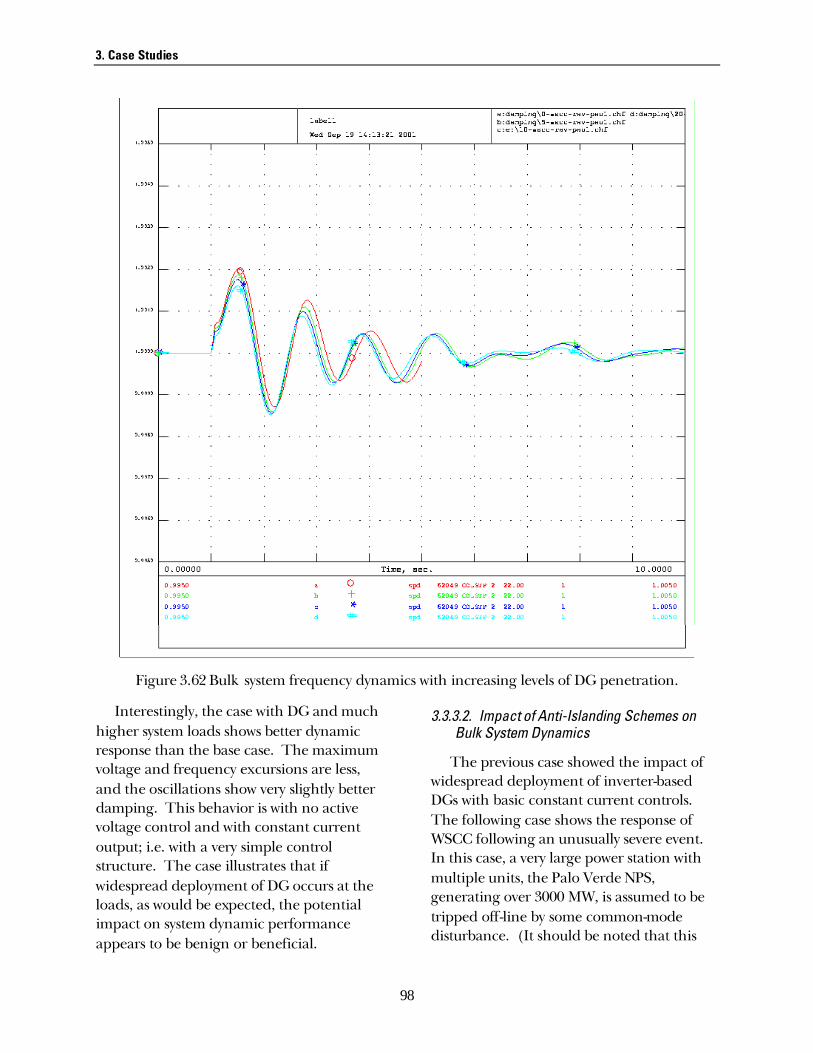
3. Case Studies

98

Figure 3.62 Bulk system frequency dynamics with increasing levels of DG penetration.

Interestingly, the case with DG and much higher system loads shows better dynamic response than the base case. The maximum voltage and frequency excursions are less, and the oscillations show very slightly better damping. This behavior is with no active voltage control and with constant current output; i.e. with a very simple control structure. The case illustrates that if widespread deployment of DG occurs at the loads, as would be expected, the potential impact on system dynamic performance appears to be benign or beneficial.

3.3.3.2. Impact of Anti-Islanding Schemes on Bulk System Dynamics

The previous case showed the impact of widespread deployment of inverter-based DGs with basic constant current controls. The following case shows the response of WSCC following an unusually severe event. In this case, a very large power station with multiple units, the Palo Verde NPS, generating over 3000 MW, is assumed to be tripped off-line by some common-mode disturbance. (It should be noted that this

3. Case Studies

99

disturbance is more severe than standard ‘N-1’ planning criteria. WSCC criteria dictate that the power system should survive this disturbance, but limited customer interruptions are allowable for events of this severity.)

Figure 3.63 and Figure 3.64 show the same two voltage and speeds as presented above. In these figures one trace (red with circles) represents the base condition, the next (green with crosses) represents a condition with twenty percent DG penetration, serving an incremental 20% of the system, and the third (blue with stars) represents a twenty percent DG penetration with all DGs equipped with the anti-islanding protection (of the type presented section 3.2.2). The case illustrates that the aggregate impact of the anti-islanding

schemes (SVS and SFS) is benign to the system performance. The voltage and frequency excursions for all cases are severe. The DG case shows a very slight improvement in voltage recovery and damping of the oscillations, and modest degradation in the recovery of the frequency. The combination of higher system load and DGs causes the slow deep system-wide frequency excursion to be somewhat worse than in the base case. This is essentially unaffected by the anti-islanding schemes. However, the anti-islanding schemes do contribute positively to damping the faster oscillatory modes of the system. This can be seen by comparing the green and blue traces in Figure 3.64. These results are specific to this particular control scheme and set of parameters.

3. Case Studies

100

Figure 3.63 Bulk system voltage dynamics with high DG penetration and impact of anti-islanding.

3. Case Studies

101

Figure 3.64 Bulk system frequency dynamics with high DG penetration and impact of anti-islanding.

3.3.3.3. Impact of DG Tripping on Bulk System Dynamics

Interconnection standards for DG, including P1547 and several state standards, include ore are trending towards the inclusion of requirements for undervoltage and underfrequency tripping of DG. These requirements are directed at ensuring that DGs rapidly disconnect in response to problems on the distribution system. However, since large-scale disturbances can

cause widespread voltage and frequency excursions, this requirement raises some concerns about its potential impact on bulk system dynamics.

Most of the new standards and guidelines dictate that DGs disconnect when voltages drop below 70% for a specified period. This maximum period generally ranges from ten cycles to two seconds. It is important to note that these documents specify the minimum voltage and the maximum time to trip. Thus, DGs will be in violation if they trip

3. Case Studies

102

slower or at too low a voltage. However, the DGs may trip faster and at higher voltages than this without violation.

The next five figures present the results of a sequence of cases in which fast undervoltage tripping of the DGs is applied. The disturbance for these cases is the same very severe event as shown in the previous case: tripping of a large multi-unit power plant. In each case there is 20% DG penetration, as described above.

Figure 3.65 shows the voltages at the 500 kV Malin bus for three conditions: The first trace (red with circles) is the base case, with no undervoltage tripping of the DGs. The second trace (green with crosses) is for DGs that are set to trip when the voltage falls below 70%. The voltage excursion for the 70% case is outside of WSCC criteria for most disturbances. The third trace (blue with stars) is DGs that trip when the voltage falls below 90%. The case with the 90% trip point is very unstable.

Figure 3.65 Bulk system voltage dynamics with low voltage DG tripping.

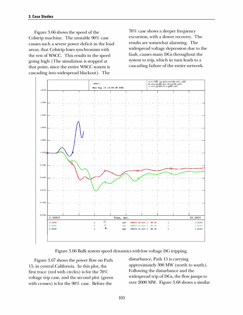
3. Case Studies

103

Figure 3.66 shows the speed of the Colstrip machine. The unstable 90% case causes such a severe power deficit in the load areas, that Colstrip loses synchronism with the rest of WSCC. This results in the speed going high (The simulation is stopped at that point, since the entire WSCC system is cascading into widespread blackout). The

70% case shows a deeper frequency excursion, with a slower recovery. The results are somewhat alarming. The widespread voltage depression due to the fault, causes many DGs throughout the system to trip, which in turn leads to a cascading failure of the entire network.

Figure 3.66 Bulk system speed dynamics with low voltage DG tripping.

Figure 3.67 shows the power flow on Path 15, in central California. In this plot, the first trace (red with circles) is for the 70% voltage trip case, and the second plot (green with crosses) is for the 90% case. Before the

disturbance, Path 15 is carrying approximately 300 MW (north to south). Following the disturbance and the widespread trip of DGs, the flow jumps to over 2000 MW. Figure 3.68 shows a similar

3. Case Studies

104

behavior on the California-Oregon interface (COI). On that interface, the flow jumps

from about 3300 MW to well over 5000 MW.

Figure 3.67 WSCC Path 15 power flow dynamics with low voltage DG tripping.

3. Case Studies

105

Figure 3.68 WSCC California-Oregon interface power flow dynamics with low voltage DG tripping.

Figure 3.69 shows the cumulative behavior of the DGs that drives the response shown in the pervious figures. This plot shows the amount of DG that is tripped due to undervoltage. Again, the first trace (red with circles) is for the 70% voltage trip case, and the second plot (green with crosses) is for the 90% case. The voltage depression during the fault causes about 1000 MW of DG to trip before the fault is cleared. Once the fault is cleared, the system voltages recovery is sufficient such that no additional

DGs trip. In the case of the more sensitive 90% trip point, approximately 5000 MW of DG (about one-quarter of the total) trip during the fault. The subsequent widespread power shortage, due to the DGs tripping, causes a cascading failure. Over the course of the next few seconds, several thousand more MW of DG trip. The exact details are relatively unimportant, since the system is beyond the point of no return within a fraction of a second following the fault clearing.

3. Case Studies

106

Figure 3.69 Cumulative DG tripping in bulk system due to low voltage.

To better understand the risk of DGs tripping in response to fault induced voltage dips, it is useful to look at the geographic distribution of voltage. Figure 3.70 shows the voltages of several 500 kV locations in WSCC, in response to the trip of entire Palo Verde station. The sequence of voltages ranges from the California -Oregon border (the deepest voltage dip) to southern California (the shallowest dip). This plot

makes it easy to see that the more sensitive the DGs (i.e., the high the trip threshold) the broader the geographic (and electric) area that will be subject to DGs tripping. It is also interesting to note that deepest voltage dip for this particular event is geographically the farthest away of the four locations plotted.

3. Case Studies

107

Figure 3.70 Bulk system geographic distribution of voltage depression due to Raver-Paul fault with DG tripping in bulk system on low voltage at 70% level.

3.3.4. Microgrid Dynamics

One business and technical structure that shows promise as a means to take full advantage of distributed generation is the microgrid. Microgrid is a loosely defined term that describes a small power system, generally with multiple generators and loads. Concepts for microgrids fall into two general categories: • Systems that are intended to always be

operated isolated from a large utility grid

• Systems that are normally connected to a larger grid.

Conceptually, the isolated microgrid is like a scaled down version of a large-scale utility grid. Many of the technical requirements are the same. In order to supply reliable, quality power, the microgrid must have mechanisms to regulate voltage and frequency in response to changes in customer loads and in response to disturbances.

3. Case Studies

108

For the grid-connected microgrid, the distinction is more subtle. The basic concept is that the microgrid be designed and operated such that it presents the appearance of a single, predictable and orderly load or generator to the grid at the point of interconnection. This arrangement provides several potential advantages for all of the stakeholders: • DG owners may be able to rate and

operate their generation more economically, by being able to export (and import) power to the microgrid.

• The microgrid takes advantage of load diversity to reduce the total installed DG capacity required.

• The load customers may be able to have continued service (possibly at a reduced level) when connection to the host utility is lost.

• The host utility may be able to depend on the microgrid to serve load customers in such a fashion that substation and bulk power infrastructure need not be rated (or expanded) to meet the entire load, as if the DG were not present. (This last point is a major, legitimate obstacle to DG.)

• The microgrid could be controlled in such a fashion as to be active asset to bulk system reliability (for example by providing spinning reserve or black start services, to name two.)

In order to realize these potential benefits the DGs in the microgrid must have, at the least, additional controls. Further, most of these potential benefits require some level of coordination and communication. These controls, which are basically aimed at making viable islands, are largely incompatible with present industry trends and the requirements of current interconnection standards.

In this section, the P2 distribution system is operated as a microgrid. This system includes many of the basic constituents of a microgrid, making it suitable for exploring many of the dynamic performance issues surrounding microgrids. The system includes multiple DGs, a range of loads with varying dynamic characteristics, and a simple grid structure (the tie between the ends of two feeders is closed for the cases presented here.)

3.3.4.1. Microgrid Dynamics with Autonomous Controls

The ability of a grid-connected microgrid to survive loss of connection to the host utility depends on a number of factors. The microgrid must have sufficient dynamic regulating capability to be able to tolerate the change in both active and reactive power flow that will result from loss of the utility tie. This means that at least some of the DGs must have both voltage and frequency regulation functions.

The following four figures show the results of a sequence of simulations on the P2 system. For these simulations, all five of the DGs on the microgrid are inverter-based devices with voltage and frequency regulation capability, limited according to their individual rating. The controls are the proportional controls presented earlier, and are autonomous, i.e. there is no coordination or communication assumed between them in the time frame of the simulation. In each case, the microgrid is disconnected from the host utility by opening the substation breaker.

Figure 3.71 shows the voltage traces at one bus (the D2 bus) for four different initial conditions: The first trace (red with circles) is for an initial condition of importing 2 MW, or about 20% of the microgrid load, from the host utility. The

3. Case Studies

109

system response is unstable for this case. The second trace (green with crosses) is for an initial condition of about 1 MW import. The third race (blue with stars) is for a nearly balanced initial condition, and the fourth trace (teal with pound symbols) is for

an initial export of about 1 MW. Figure 3.72 shows the corresponding frequency traces. Figure 3.73 shows the active power output of one of the DGs, and Figure 3.74 shows the reactive power output of that same DG.

Figure 3.71 Microgrid voltage at Bus D2 following islanding from bulk system.

3. Case Studies

110

Figure 3.72 Microgrid frequency following islanding from bulk system.

3. Case Studies

111

Figure 3.73 Active power output of DG at Bus D2 following microgrid islanding from bulk system.

3. Case Studies

112

Figure 3.74 Reactive power output of DG at Bus D2 following microgrid islanding from bulk system.

There are several observations that can be made. The most obvious is that the microgrid can operate stably following disconnection from the grid with autonomous proportional controls, as long as the power export (or import) preceding the disturbance is not too large. For this case, ‘too large’ was somewhere between 1– 2 MW (or roughly 10 and 20% of the microgrid load). In general, to be viable the DGs on the microgrid must have sufficient range to pickup the change, and they must

respond quickly (and stably). In other words, the microgrid must act like a regular utility grid—at least in this time frame.

The behavior of an isolated microgrid presents similar requirements. Again, as with a large conventional utility grid, the isolated microgrid must retain sufficient regulating reserves to allow it to respond to system disturbances. One disturbance that the microgrid must tolerate is loss of one of the DGs.

3. Case Studies

113

Figure 3.75 shows the response of the P2 system to trip of one DG. Unlike the previous sequence of cases, the initial condition for this disturbance was already islanded. The figure shows four traces. The disturbance is trip of one DG, which is initially producing about 1.5 MW. The first trace (red with circles) is the active power output of one of the four remaining DGs. The second trace (green with crosses) is the reactive power output of the same DG. The third trace (blue with stars) is the frequency. The fourth trace (teal with pound symbols) is the terminal voltage of the same DG.

The response shown in Figure 3.75 is relatively complex. To understand the response, it helps to remember that the inverter-based DGs are limited in the current that they can deliver. In this disturbance, loss of the DG initially causes the frequency on the microgrid to drop rapidly. This can be seen clearly in the first half second following the DG trip (blue trace is dropping). The frequency regulation function (governor function) responds by increasing the active power output of the DG (red trace rises in the same time period.) In the same time period, the voltage (teal) steps up but then begins to decline as well. The voltage regulation function responds initially by dropping the reactive power output, but then boosting it as the voltage declines (green). Just before two seconds, a dramatic

change occurs. This is because the DG inverter has run into its current limit. At this point, this particular control is designed to give active power priority over reactive power. Therefore the reactive power drops to zero (green) trace, and the active power current is pegged at the maximum until about three seconds. The active power (red) droops a bit in the middle of this time period, because the voltage (teal) drops abruptly in combined response to the system swing and the reduction in reactive power output. (The active power output is the product of the active power current, which is pegged, and the voltage which droops.) The system survives the swing, and inverter comes out of current limits at about three seconds, restoring the voltage regulation function as well.

This case helps illustrate several points of interest. First, it is possible for microgrid with autonomous DG controls to tolerate upsets and operate stably. Second, it shows that the behavior of the DGs when pushed against limits can be an important factor in whether a system survives an upset. The case illustrated shows only one possible control response to hitting limits. Others could be devised and have been proposed. It is not clear from this one example, which control strategy is most robust and likely to give the best performance over the widest range of possible conditions.

3. Case Studies

114

Figure 3.75 Response of to trip of one DG on microgrid initially operating islanded.

3.3.4.2. Microgrid Dynamics with Supervisory Control

The cases above show that autonomous controls of DG hold promise for providing acceptable dynamic performance in the time immediately following system upsets. Coordinated or supervised control may widen the window of events that can be successfully tolerated by the microgrid. Another aspect of microgrids mentioned in the introduction to this section, is the potential to provide a controlled and limited

burden on the host utility. In order for the entire microgrid to present such a limited burden requires some type of supervisory control. In this section, one such supervisory control is tested.

The case shown here is the microgrid response to a load trip. For this case, the micro grid initially exports power to the host grid. The supervisory controller is based on a typical automatic generation control (AGC) that would be used to control power exchange between two bulk power systems. In this case, the objective of the supervisory

3. Case Studies

115

control is to quickly return the power exchange between the microgrid and the host grid to a specified level. The traces in Figure 3.76 show (1) the power exchange with the grid, measured at the substation (the green trace with crosses) and the (2) power command signal sent to the DGs within the microgrid that are under supervision. For this control, deviation of the power exchange with the grid from the initial condition provides the input signal (error) to the controller. The output signal commands the DGs on the microgrid to adjust their output—downwards in this case.

For this event, the power is returned to the scheduled level within a minute. This response could be made faster or slower, depending upon the physical and contractual requirements of the systems. Appendix G in [5] includes figures with show voltage, frequency and active and reactive power traces for this case.

This case illustrates that a microgrid could be controlled in a similar way to that of a large utility grid, so as to minimize the microgrid’s impact on the host utility.

Figure 3.76 Power exchange and control response to load trip within the microgrid with power balancing supervisory control.

3. Case Studies

116

3.3.5. Power System Dynamics Summary

The presence of distributed resources on the power system has the potential to affect system dynamics. Several cases were presented in this section, which help illustrate these effects. The cases cannot be considered comprehensive enough to allow definitive conclusions to be drawn, however, several observations about the behaviors presented can be made:

Observations on local dynamics • Local distribution system dynamics are

most affected by DGs trips. • DG controls do not have a major impact

on local dynamics when the connection to the host utility is maintained.

• Anti-islanding schemes (of the type studied here) appear to be effective at destabilizing islands containing multiple DGs and loads with relatively complex dynamics.

• Voltage and power regulation tend to act contrary to the anti-islanding schemes.

Observations on bulk system dynamics • Widespread penetration of DGs at the

load appears to be benign with respect to system response to bulk system disturbances.

• Anti-islanding schemes (of the type studied here) appear to have little impact on system response to bulk system disturbances.

• Aggressive tripping of DGs in response to undervoltages appears to present a substantial hazard to the bulk system, and was shown to bring down the entire U.S. western system in one extreme case.

Observations on microgrid dynamics • Microgrids appear to be viable, within

limits, when DGs are provided with fast

autonomous voltage and frequency controls.

• Microgrid supervisory control was shown to provide satisfactory performance in terms of managing power exchange with the host utility (for one illustrative case.)

3.4. Summary

As part of this program’s effort to develop a DG-EPS interconnection interface box that allows DG sources to be interconnected to the EPS, various DG-EPS interconnect cases were studied by conducting simulations utilizing the GE-designed VTB as described in Section 2 and [4]. The results from these case studies will enable us to make recommendations for improvement to the IEEE P1547 standard as well as provide inputs to the design of the interconnection interface box.

The set of simulations run on the VTB were based on a case list compiled by the team from various brainstorming sessions, IEEE P1547 Draft Standard, Edison Electric Institute Distributed Resources Task Force Interconnection Study, and literature searches. The cases studied are grouped into two categories: power quality case studies and protection and reliability case studies.

The power quality case studies include: • Voltage regulation • DG design considerations to meet power

quality requirements: - Harmonics - Flicker - DC current injection - Grounding - Unbalanced grid

The protection and reliability case studies include: • Transient response and fault behaviors:

3. Case Studies

117

- Capacitor switching - Fault Behaviors

• Reclosing • Anti-islanding studies • Power systems dynamics and stability

Some key findings from these initial studies of the impact of DG-EPS interconnect include the following: • Widespread penetration of DGs at the

load appears to be benign with respect to system response to bulk system disturbances.

• With significant levels of DG penetration, it will be difficult to avoid detraction from EPS voltage regulation performance. While the Draft IEEE P1547 presently requires that a DG not cause the EPS voltage to fall outside of the prescribed regulation range, achieving this goal may become increasingly difficult using conventional approaches. EPS voltage regulation performance problems due to DG can be mitigated if there is integrated control of system voltage and reactive power management. IEEE P1547 may need to incorporate provisions where the reactive power output of the DG is controlled by the EPS operator.

• Simultaneous tripping of DGs in a system dependent on the DG output can result in widespread and severe voltage problems. Presently, P1547 is biased in favor of fast tripping in order to rapidly detect and eliminate inadvertent islands. There may need to be further consideration of the fine balance between island avoidance and making the system vulnerable to voltage collapse. Avoiding overly aggressive DG tripping should be a design objective.

• Anti-islanding schemes (of the type studied in this project) appear to be effective at destabilizing islands containing multiple DGs and loads with relatively complex dynamics while having little impact on system response to bulk system disturbances. Some analytical techniques used to design and test anti-islanding schemes are unrealistic and potentially misleading. This is a highly complex subject, and further investigation is highly desirable.

• Inverter-type DGs will have significant beneficial impact on flicker caused by system loads, only if they have a voltage regulation function or if they have a control scheme where they are operated as controlled voltage sources (i.e., as virtual synchronous generators).

• Modern inverter-based DGs do not contribute to system fault current beyond the pre-fault operating current level. However, the current contribution of the DG system to a single phase fault may be greater than the three phase case which conflicts with IEEE P1547 requirement that ground fault current contribution of a DG shall not be greater than 100% of the fault current contribution of the DG to a three phase fault. This is because the DG is a nearly ideal current source for the positive sequence, but is generally a constant impedance or voltage source for the zero sequence. Both are desirable characteristics, and the result reveals that the wording of P1547’s single-phase to three phase fault current ratio requirement is more appropriate for conventional rotating generators. The wording of this requirement needs additional consideration with respect to its consistency with inverter-based applications.

• Take-aways for future DG designs:

3. Case Studies

118

- Single phase Sandia Anti-islanding scheme can be effectively extended to 3 phase DG systems;

- Inverter based DGs will have significant beneficial impact on flicker only if they include a voltage regulation function;

- DG voltage regulation functionality may be beneficial in reducing the impact of DG penetration on EPS voltage regulation performance. However, local control may not be sufficient and a system level voltage control approach may be necessary in many applications.

- DG voltage regulation may reduce the effectiveness of active anti-islanding schemes.

- Transformer-less DGs should pay special attention to zero-sequence impedance design so an effective ground can be provided.

The GE-designed interconnect interface box will address some of the issues identified above, such as integrated control of system voltage; reactive power management; and communication to a supervisory level to manage microgrid power exchange.

119

4. Conceptual Interconnect Design

4.1. Introduction

4.1.1. Interconnect Needs and Issues

Traditional non-utility generated power sources, such as emergency and standby power systems, have minimal interaction with the electric power system. As Distributed Generation (DG) hardware becomes more reliable and economically feasible, there is an increasing trend to interconnect those DG units with the existing utilities to meet various energy needs, as well as to offer more service possibilities to customers and the host EPS. Among these services are (1) standby/backup power to improve availability and reliability of electric power; (2) peak load shaving; (3) combined heat and power; (4) the ability to sell power back to utilities or other users; (5) power quality, such as reactive power compensation and voltage support; and (6) dynamic stability support, to name a few. This trend is fueled and accelerated by utility deregulation.

However, a wide range of system issues arise when the DG units attempt to connect to the Electric Power Systems (EPS). Major issues regarding the interconnection of DG include protection, power quality, system reliability and system operation. Another complex issue is interconnection cost, which involves equipment design, industry standards, and the local utility’s approval process. These are some of the issues that have been identified as barriers to the application of DG in the EPS [1]. The solutions to these technical challenges will help not only shape the future of electric power generation, transmission, and

distribution systems, but will also have a profound impact on the economics.

Previous sections of this report were focused on the analysis of the technical challenges to DG penetration. This section uses the previous results to recommend how distributed generation features can be designed for interconnection with the EPS. The section also outlines concepts for the design of reliable and cost effective interconnect hardware to help address these barriers.

4.1.2. Reliable and Low Cost Interconnect Solution

To promote the application of distributed generation, the following steps need to be taken. First, a widely accepted interconnection standard is needed that will allow for a standardized, cost effective interconnection solution. The IEEE SCC21 P1547 standard working group is currently working towards this goal. Second, new technical requirements that address the emerging needs of DG for dispatch, metering, communication and control should be fully explored. These additional features will improve the value of DG and the performance of the system.

The objective of this report is to conceptualize the elements of a new interconnect solution that supports a reliable and standard product design. In general, equipment vendors already exist that package the physical current carrying components (e.g., switches and circuit breakers) suitable for DG applications. These interconnection elements are already well covered by existing product lines and commonly available in industry. Of


120

necessity, these elements of the interconnect will vary considerably in size and packaging based on the specific DG technology and application. However, there are other interconnect elements that offer some potential for standardization and improved functionality. Consequently, we will focus this report on the structure and implementation of the protection, monitoring and control elements that leverage these existing products.

The section is outlined as below: • DG and interconnect improvements:

This section will capture the implications and improvements identified in the case studies. Anti-islanding control schemes are highlighted as a unique and critical function of the DG interconnection.

• Survey of interconnect standards: Results of the survey of current interconnect standards are tabulated to help clarify the underlying interconnection requirements for different applications and technologies.

• Conceptual design of an interconnect interface: In this section, a brief overview of current industry interconnect product is presented. The future interconnect needs and trends are discussed. A conceptual interconnect interface design is presented that incorporates the following features: - A core protective and control

functional block suitable for most grid-connected DG applications; These functions are intended for P1547 compliance.

- Different layers of functionalities are identified and will be incorporated in a multi-generation interconnect development.

- The design is based on a modular approach with normalized interfaces.

- Adjustable settings and scalable components.

- Open architecture to be easily integrated into existing utility hardware and software.

A design example to illustrate the concept is also provided.

4.2. DG and Interconnect Design Improvement

4.2.1. Implications From Case Studies

Based on case studies, a number of DG/EPS interconnection issues were discussed and analyzed. The results of the analysis provide direction for DG and interconnect improvements. This section summarizes the issues, improvements and recommendations with respect to power quality, reliability and protection.

4.2.1.1. Power Quality Improvements

Voltage regulation

Issues: The maintenance of the voltage within an acceptable range at the point of delivery to each customer may be affected by Distributed Generation. Without DG, power flow in a radial distribution2 system is always unidirectional, and monotonically decreasing in real power (kW) magnitude with increasing distance from the substation. The addition of DG to a system, however, can radically shift power flow patterns and make them unpredictable. This is particularly true when interconnection policies and regulations allow DG operators to export power into the grid, or cease export, at will.

2 Radial distribution is used to supply the vast majority of US

distribution loads. While looped feeders (feeders connected to substations at both ends) are often encountered, they are almost always operated with an open point, separating the feeder into two radial sections.


121

Depending on the spatial relationship of loads and DG, power flow can increase or decrease along a feeder. Net power flow can potentially reverse over a portion of the feeder, or even over the entire feeder if DG production exceeds the load present at that time. These load flow variations can make it difficult to maintain adequate voltage regulation. Also, the unconventional load flow patterns can cause distribution system voltage regulation devices, such as step voltage regulators, load tap changers, and switched capacitor banks to respond inappropriately.

Regulation of local voltage by the DG can be detrimental or beneficial to the overall voltage regulation on the distribution system. In order to provide adequate voltage regulation over the extent of the distribution system, the desired voltage at the DG location may need to vary with (1) system loading conditions, (2) status of system voltage regulation and reactive compensation equipment, and (3) changes in the distribution system topological structure (which may vary in the course of normal operations). Thus, local information alone may not be sufficient to regulate voltage as required by the needs of all the consumers connected to the distribution system.

Improvements/Recommendations: Early drafts of the P1547 standard did not allow a distributed generator to regulate voltage, effectively requiring operation at a constant power factor or reactive power output. While later drafts of this standard do allow voltage regulation, it is generally perceived to be unwise to attempt grid voltage regulation with a DG.

With significant levels of DG penetration, it will be difficult to avoid detraction from EPS voltage regulation performance. While

IEEE P1547 presently requires that the DG shall not cause the prevailing voltage level of the area EPS at the PCC to frequently go outside of ANSI C84.1 Range A, simply maintaining voltage at the PCC to an arbitrary point within Range A does not necessarily benefit EPS voltage regulation over the feeder.

For example, consider a DG located immediately downstream of a voltage regulator. The regulator’s voltage drop compensation needs to raise the voltage on its downstream side to the upper end of Range A during heavy-load conditions to ensure that adequate voltage is provided to customers at the end of the feeder. If the DG regulates voltage at this location to the nominal voltage, then the necessary control of feeder voltage is not achieved. In addition, because the regulator’s control objective is not achieved, it may go to the maximum tap position, forcing voltages upstream of the regulator to unacceptably low values. If the DG should trip, the regulator tap setting might then cause downstream voltages to be excessive until the tap setting is readjusted.

EPS voltage regulation performance problems due to DG can be mitigated if there is an integrated control of system voltage and reactive power management. This could be a functional requirement for the DG and interconnect.

Flicker

Issues: The repetitive and rapid changes of voltage have the consequence of causing unacceptable variations in light output and other effects on power consumers and their equipment. DG may either introduce flicker or mitigate flicker. The usual cause for DG-induced flicker is variations in the DG’s prime mover power output. Examples are fluctuations of wind turbine output due to


122

gusting and variations in a photovoltaic system power output due to passing cloud shadows. Flicker is not an issue for most DG applications, however. Flicker is more often caused by rapid load variations. A DG can mitigate load-induced flicker by compensating for abrupt changes in real and reactive power demand of a flicker-causing load.

Improvements/Recommendations: The study has shown that a DG can mitigate load-induced flicker, as summarized below: • Inverter based DGs operating in a

constant current mode without voltage regulation functions have a very slight inherent benefit on flicker performance.

• Inverter based DGs have the potential to provide substantial benefit regarding flicker if equipped with controls that provide voltage regulation or some other functional equivalent.

• Rotating equipment, including DGs using synchronous or induction generators, increases short circuit strength and therefore improves flicker performance.

• Additional control of rotating equipment is relatively ineffective at further improving flicker performance.

Voltage unbalance

Issues: The grid voltage usually does not display identical voltage magnitude on each phase, and shows a 120-degree phase separation between each pair of phases. The voltage unbalance may impact inverter-based three-phase DG designs. Since the DG is controlled as a balanced (positive-sequence) current source, the product of positive-sequence current and the unbalanced (negative-sequence) voltage will cause two-times-fundamental frequency power ripple. This 120 Hz ripple will appear at the inverter

input DC bus, mainly in the form of ripple current. The DC bus voltage is much less affected due to the bulk DC bus capacitor in a normal design. The voltage unbalance will also affect DG phase-lock loop (PLL) performance.

Improvements/Recommendations: Typically, three methods are used to obtain accurate PLL output when there is a voltage unbalance. • Low pass filter: The cutoff frequency is

one order lower than 120 Hz. This normally requires the PLL bandwidth to be around 10 Hz.

• Notch filter used to filter 120 Hz: This way, the bandwidth of PLL can be higher than the method above.

• Algorithm to obtain only positive-sequence voltage information and use it as PLL input: This way, the current reference is only synchronized with positive-sequence voltage.

Harmonic distortion

Issues: The injection of currents having frequency components that are multiples of the fundamental frequency. All power electronic equipment creates current distortion that can impact neighboring equipment.

Improvements/Recommendations: The harmonic issue with DG is primarily an equipment vendor design and application issue. Hence, it is a requirement of the DG design that the harmonics be below acceptable limits. Some interconnect control, such as anti-islanding, may introduce additional harmonic distortion, which should be examined and limited. If the additional harmonic distortion is significant, an alternative anti-islanding solution may have to be used. This subject will be covered in a separate section.


123

Direct current injection

Issues: When DG power converters are directly connected (without isolation transformers) to the utility grid, there is the potential to inject DC current. This can cause saturation and heating of transformers and motors, and additionally can cause these passive devices to produce unacceptable harmonic currents. Continuous DC voltage injection may also result during some internal DG power converter faults.

Improvements/Recommendations: The protection of the system must be designed to clear such conditions. In grid-parallel mode, DC current injection limits are typically met by DG control functions. In stand-alone operating mode, the output DC voltage and its integral should be limited. This is to ensure that loads with low DC impedance such as machines and transformers do not saturate.

DG Grounding

Issues: A DG connected to a four-wire EPS, whether directly or through a transformer, should provide an effective ground to prevent unfaulted phases from overvoltage during a single-phase to ground fault.

Improvements/Recommendations: For a DG with an output isolation transformer (delta-wye) to interface with the grid: • When the grid is connected, the grid

source will provide a grounding source (sufficiently low zero-sequence impedance). Therefore, the system is still effectively grounded.

• When the grid is disconnected, the grid source sequence impedances are no longer part of the circuit. The grid wye-wye distribution transformer provides a series path for zero sequence, but does not provide a grounding source.

Therefore, a grounding source with an appropriate zero-sequence impedance should be provided on the secondary.

• The DG isolation transformer provides a shunt zero-sequence path to the load zero sequence impedance. The transformer shunt zero-sequence impedance is normally low enough to provide effective grounding. However, the low zero-sequence impedance transformer may be subject to overload due to system unbalances, such as faults, open phases, etc. In this application, the transformer zero-sequence impedance must be designed such that an effective ground can be provided, while it can also withstand system disturbance. This is a tradeoff in the DG transformer design.

For DG without an output isolation transformer, a grounding source must be provided. This could be fulfilled by either using a four-leg inverter (or other topologies providing three-phase four-wire output without an output transformer), or a separate grounding transformer: • When the grid is connected, the grid will

provide a grounding source so the system is still effectively grounded.

• When the grid is disconnected, the four-leg inverter should be designed such that a low zero-sequence impedance Z0(INV) is obtained for the DG to provide an effective ground.

If the distribution transformer has a delta or floating-wye primary (EPS side), the required grounding cannot be provided by the inverter or any other device connected to the secondary side. Alternatives for providing primary system grounding in the event of separation of the EPS from its normal source are to: • Replace the distribution transformer

with one having a connection providing


124

a primary ground source or one that connects the primary and secondary zero sequence, plus provide grounding on the secondary side.

• Provide a parallel grounding source on the primary.

An alternative to providing a primary ground source, achieving the same functional goal, is to monitor the primary side phase to ground voltage, and instantly discontinue inverter operation in the event of an overvoltage.

4.2.1.2. Reliability and Protection Improvements

Anti-Islanding

Issues: Islanding of a grid-connected DG occurs when a section of the utility system containing such generators is disconnected from the main utility, but the independent DGs continue to energize the utility lines in the isolated section. Unintended islanding is a concern primarily because it poses a hazard to utility and customer equipment, maintenance personnel and the general public. Other concerns are poor power quality that can damage loads in the island and possible out-of-phase switching of the feeder recloser leading to damage to the DG, neighboring loads and utility equipment.

Improvements/Recommendations: • The DG without active anti-islanding

control has the potential to island for a subsystem where net real and reactive power demand and generation are in balance.

• Some active anti-islanding methods may work well for some loads (e.g., RLC loads) but appear to be inadequate for induction motors with large inertial loads that include significant reactive compensation. More research is needed

to fully quantify these loads and to investigate anti-islanding alternatives.

• Simultaneous tripping of DGs in a system dependent on the DG output can result in widespread and severe voltage problems. Presently, IEEE P1547 is biased in favor of fast tripping in order to rapidly detect and eliminate inadvertent islands. There may need to be further consideration of the fine balance between island avoidance and making the system vulnerable to voltage collapse. Alternatives to reliance on out-of-range voltage and frequency as the primary means of island detection should also be given further consideration. Avioding overly aggressive DG tripping is an important design objective.

Reclosing

Issues: Reclosing of breakers after a temporary fault is a common practice to prevent extended interruption of supply to customers. The fault clearing breakers are delayed from closing after a fault to allow the fault path to deionize. The reclosing time delay varies widely from system to system, and typically, the delay also increases for subsequent reclosing attempts. If an island is created and maintained, the difference in the frequency between the islanded DG/load system and the grid can result in out-of-phase reclosing. Although the possibility of this occurring is remote, when it occurs, the impact on the system is very severe. For example: • There is the potential for high peak

voltages during reclosing that can affect surge arrestors in the utility system as well as connected customer loads.

• High motor and transformer inrush currents caused by out-of-phase reclosing can trip other breakers and blow fuses in the system.


125

• Large mechanical stress can be placed on mechanical system driven by motors.

• Mechanical stress can be placed on the DG, particularly if it uses a rotating generator.

Improvements/Recommendations: To prevent out-of-phase reclosing, effective anti-islanding controls should be incorporated so that the DG will trip off-line before a reclosing event can take place.

Power system dynamics

Issues: The presence of distributed resources on the power system has the potential to affect system dynamics. In analysis of bulk power systems, the presence of distributed generation has normally been aggregated, or netted out, with the loads. However, the response of distributed generation to perturbations of voltage and frequency, and more importantly, to large disturbances such as faults, is potentially very different from that of loads. Thus, when systems begin to have significant penetration of DGs, a wide range of fundamental (power) frequency issues arise, such as: • Transient stability (maintenance of

synchronism) • Dynamic stability (damping of electro-

mechanical oscillations between generators)


Improvements/Recommendations: The observations from power system dynamic studies, considering inverter-interfaced DG, are summarized below:

Observations on local dynamics

• Local distribution system dynamics are most affected by DG trips.

• DG controls do not have a major impact on local dynamics when the connection to the host utility is maintained.

• Anti-islanding schemes (of the type studied [2]) appear to be effective at destabilizing islands containing multiple DGs and loads with relatively complex dynamics.

• Voltage and power regulation tend to act contrary to the anti-islanding schemes.

Observations on bulk system dynamics

• Widespread penetration of DGs at the load appears to be benign with respect to system response to bulk system disturbances.

• Anti-islanding schemes (of the type studied [2]) appear to have little impact on system response to bulk system disturbances.

• Aggressive tripping of DGs in response to undervoltages can present a substantial hazard to the bulk system in high penetration cases.

Observations on microgrid dynamics

• Microgrids appear to be viable, within limits, when DGs are provided with fast autonomous voltage and frequency controls.

• Microgrid supervisory control was shown to provide satisfactory performance in terms of managing power exchange with the host utility.

•

4.2.2. Anti-Islanding Control

One unique protective control of DG is anti-islanding. There are a number of methods existing today [25-47]. This section


126

first presents the background of the anti-islanding issue. Then, the design considerations and future work of anti-islanding control design are discussed. A survey of existing anti-islanding methods and their comparison is in Appendix A in [6].

4.2.2.1. Background

EPS EPS breaker

DG disconnect

DG

Load

EPS EPS breaker

DG disconnect

DG

LoadLoad

Figure 4.1 An EPS with DG.

Islanding occurs when a DG system feeds power into a section of an EPS system that has been isolated from the EPS source. In general, the isolated section will contain a number of loads, with the loads connected to the feeder through distribution transformers. Some transformers may serve individual loads, other transformers serve several customer loads. For simplicity, consider the configuration in Figure 4.1, a DG system connected to a feeder through a transformer. A load is also connected to the same feeder through another transformer. The DG is supplying a nearly sinusoidal current with the same frequency and phase (if unity power factor) as the voltage at the DG terminal. If an EPS switching device (circuit breaker, recloser, fuse, or sectionalizer) opens, it is possible for the DG to continue to supply current to the isolated section of the EPS. This is islanding, and the isolated section of the EPS being powered by the DG system is referred to as

an island. Continued existence of an operating island generally requires that the real and reactive power output of the DG is approximately equal to the real and reactive power demand of the load connected to the isolated section.

The primary concerns with islanding are: • Public safety: Fault detection and

protection systems may not be operable or coordinated. Most distribution system protection systems require the presence of a significant source of short-circuit current for the devices to operate. A DG sourcing the islanded section may be too weak to provide enough short-circuit current capacity for protective devices (overcurrent relays, reclosers, fuses) to operate.

• Personnel safety: Maintenance or repair personnel arriving to service the isolated feeder may be unaware that it is still energized, which could lead to personal injury.

• Power quality: The EPS operator is responsible for the quality of power provided to all customers. Islanding removes EPS control of voltage and frequency provided to customers on the islanded section. It is possible for customers to be subjected to extreme voltage conditions, while voltages at the point of DG interconnection are within the normal range. This poses issues of liability, performance with respect to regulatory requirements, contractual obligations, safety, equipment damage, and equipment mis-operation.

• Equipment damage due to out-of-phase reclosing: The DG system, which relies on the EPS voltage to provide phase and frequency reference for its output current, may lose synchronization with the EPS while the EPS is disconnected.


127

The frequency and phase of the DG output current may drift away from the EPS voltage frequency and phase. The phase difference is particularly serious because the EPS switching device may reclose on the out-of-phase island, causing surge voltage and current, which could quickly damage the equipment of the utility, DG or load.

• Interference with EPS protection: If the DG runs on after the EPS breaker opens due to a temporary fault within the local section of the EPS, the fault current contribution from the DG may cause mis-coordination of EPS protections. Consequently, an otherwise clearable temporary fault may become a permanent outage.

• Delay of maintenance and system restoration: Prior to initiating maintenance or repair on the primary system, safety rules require that the system be verified as being de-energized, unless hot-line procedures are used. If a DG is energizing a portion of the system after the normal EPS source has been disconnected, work cannot begin until the source of energization is identified and secured.

• As the DG penetration in the power system increase, the DGs will have an increasing impact on the power system’s voltage and frequency stability. Hence, it is important that the DGs do not trip unnecessarily during system disturbances and that they continue to provide real and reactive power support. Therefore, it is important that the anti-islanding algorithm be able to differentiate between a true islanding situation where rapid disconnection from the grid is necessary, and other system disturbances where DG disconnection is not necessary

and may be deleterious to system stability.

Due to the significance of the anti-islanding protection, researchers have proposed a number of methods, passive or active. All of them have merits and disadvantages. This document summarizes the existing methods reported in papers and patents. Their principles and implementations, and the comparison of their basic features are described in Appendix A in [6].

4.2.2.2. Anti-Islanding Design Considerations

In general, an islanding prevention method should accomplish the following goals: • Detect islanding rapidly enough to

guarantee personnel and equipment safety and safeguard the reliability and integrity of the EPS and DG systems;

• Disconnect the DG system only when an island has actually occurred to avoid nuisance trips;

• Detect islanding and disconnect the DG system from the EPS, regardless of the initial state of the system (light or heavy load), composition of the load, or presence of other DGs;

• Minimize or eliminate any compromise between the effectiveness of anti-islanding detection and DG/EPS system power quality;

• Minimize hardware requirements to reduce DG interconnection cost;

• Minimize or eliminate any interaction with normal EPS operation and control.

The survey in Appendix A in [6] shows that not a single existing anti-islanding method can accomplish all of these goals simultaneously. In fact, examination of these schemes indicates that many of them are impractical in a realistic power system


128

operating environment. Therefore, there is a need for further research on anti-islanding or some other means to achieve the same objectives.

Basically, there are several topics for further investigation. • How to define the effectiveness of anti-

islanding methods: One concept is Non-Detection Zone (NDZ) based on RLC load. However, in the real world, the probability of encountering a purely RLC load is very low. Motors constitute a large part of the typical system load, and their complex dynamic behavior is not well represented by an RLC circuit. The evaluation of NDZ may have very little practical value, and may be misleading in some ways. A new methodology to evaluate the effectiveness of anti-islanding methods should be established to reflect real world situations.

• Each anti-islanding method is a function of many factors of DG/EPS/Load systems. There is no report on parameter optimization of any existing methods.

• The comparisons of the existing schemes are mostly qualitative. More quantitative results are needed to complete the comparison.

• A successful anti-islanding method should be effective for the worst-case system conditions. A particular system condition could be a worst case for one anti-islanding method, but not a problem for another anti-islanding method. This leads to a view that combined schemes may be more effective than a single one. Then, the issue is how to choose an appropriate combination with no counteracting effects on each other.

• Most anti-islanding methods assume the DG is controlled as a current source. This is practical only with inverter-interfaced DG. In some cases, inverter-interfaced DG may have some level of voltage regulation to improve other performances, such as flicker, feeder voltage regulation, etc. In addition, there are DG inverter control schemes where the DG appears to the system as a virtual synchronous machine. It is understood that DG with voltage regulation tends to sustain an island, imposing more of a challenge to anti-islanding. There is no literature existent addressing anti-islanding protection of DG with voltage regulation, or with these alternative control schemes.

4.3. DG/EPS Interconnect Standards and Requirements

4.3.1. Background

The requirements of an interconnect interface depend on technical factors related to the DG and the system to which it is connected. Additional requirements are dependent on interconnection standards imposed by the utility to which the DG is connected and by the regulatory authority having jurisdiction in that locale.

While there are efforts underway to develop IEEE P1547 as a uniform standard defining interconnection requirements, this standard, even after approved as an IEEE document, is not binding. It may be binding if adopted by a regulatory authority, but there is ample precedent of local authorities applying their own modifications to standards. Also, the current draft of P1547 provides some very general requirements, which leave substantial latitude in interpretation and application, and this may generate specific requirements by


129

interconnecting utilities as fulfillment of the general requirements. At present, a number of state regulatory authorities have developed their own standards independent of the IEEE effort. These states may withdraw their requirements and replace them with the requirements of P1547 when it is adopted, or harmonize their requirements with P1547. However, this is not guaranteed. There could be action imposing a national standard on the federal regulatory level, but the federal jurisdiction over distribution systems could be subject to legal question. Even with a mandatory national standard, the details of implementation will need to conform to the technical realities of the specific application, including: • Generator type • Size of generator relative to the capacity

and short-circuit strength of the utility system at the point of interconnection

• Type of distribution system (e.g., radial, network, etc.)

• Location in the distribution system • Distribution system protection scheme.

Thus, it is important for the DG interconnection device to fulfill the common requirements of existing interconnection standards, as well as the flexibility to provide the known or reasonably anticipated requirements dictated by local technical conditions or local interconnection requirements. Also, attention must be given to the future interconnection requirements. In most of the DG interconnection standards in effect today, there is an implicit assumption that the DGs are point applications with low penetrations. The requirements of today’s standards may actually be in contradiction with what is needed to accommodate future widespread application of DG with higher system penetration, and to exploit the capabilities

of the DG to support overall system reliability and performance.

The general requirements of all the utilities emphasize the needs of safety, reliability and power quality. However, the specific requirements of each standard vary depending on the operating practices of that utility, or due to historical factors in the development of the various standards. A survey was made of existing Interconnect Standards [47-60] (a list of which is attached in the Appendix B in [6]). The main emphases were: • The common requirements among

different standards. The common requirements help understand underlying requirements for interconnecting different DGs to different utilities and locations.

• Dissimilarities between the standards. The dissimilarities help understand application variations.

4.3.2. Common Requirements in Different Standards

The common requirements for most of the standards are listed below:

4.3.2.1. Isolating Switch

One of the major concerns of a utility is the safety of its personnel, in the case of accidental energization of a supposedly dead line due to the presence of a DG. OSHA work rules require that a circuit cannot be worked on using dead-line techniques unless all sources are visibly disconnected and locked open. Otherwise, live-line work techniques are required, which can significantly add to time required for maintenance and service restoration. Hence all the utilities need a readily accessible, lockable, visible-break isolation device to be located in between the area EPS and the DR unit.


130

This device shall be properly rated for the application. Typical ratings of the switch include: a) rated load current, b) short time current rating, c) rated voltage. This is in addition to fault clearing breakers needed for the DG. The switch would need an interlock with the DG breaker, so that it cannot be closed onto the system, unless the DG breaker is open. This is to prevent the DG being paralleled with the grid without synchronization.

4.3.2.2. Protective Relays

The presence of DGs in a system changes the system power flow pattern and protection. This basically depends on the nature of the system to which the DG has been interfaced. However, a few common requirements still exist which need to be fulfilled by the DG regardless of the system to which it is connected. DGs that are designed to work in parallel with a grid have to adjust the voltage and frequency of their output according to the variations in the utility system. Each utility specifies its own nominal system parameters, depending on its operating procedures. Deviations from nominal voltage and frequency have to be detected and the DG disconnected from the system under such conditions. This requires the presence of over/under voltage and over/under frequency relays. To enable the variations in the settings requirement, the relay should have an easy user interface with adjustable voltage or frequency threshold and time delay settings ranges, preferably with a resolution of 0.1 Hz for frequency and 2 Volts (on a 120 V base) for voltage. Also the settings should be accessible to authorized personnel only. The number of distinct levels for the setting is variable in all the standards and should allow for at least 3 ranges to be compatible with the various standards.

The relay settings are determined by the size of the DG. Relatively large generators are generally allowed more variation in the settings to prevent them from tripping and further aggravating system frequency excursions. Some of the utilities accept voltage and frequency relaying as sufficient for anti-islanding protection, especially for smaller DGs, while others require dedicated anti-islanding controls.

The DGs that are not intended to supply power to the grid need to be protected by a reverse power flow relay. This can also be used to avoid an islanding condition. The setting of the reverse power relay should be lower than the minimum net load (connected load minus DG output under that condition) that would be expected at the PCC. In case the DG is exporting power to the grid, this relay could be used as an additional logic for blocking or changing under-frequency trip setpoints of the DG.

4.3.2.3. Anti-Islanding

All the utilities emphasize that the DGs should not island with some of the grid load and hence, create a hazard for the system or personnel. Protection against this is termed as anti-islanding and is a requirement of all the utilities.

4.3.2.4. Synchronization

Synchronization and reconnection to area EPS is a required function for most DGs. Different types of DGs have different synchronizing methods. For synchronous generator, there are manual and automatic synchronizing methods. To interconnect an induction machine, most utilities require speed matching, i.e. the induction machine is brought close to synchronous speed and the breaker is closed. For inverters, the synchronization usually is automatic in that the grid frequency can be tracked by the


131

phase lock loop, which is part of inverter control. If the inverter is in locally islanded operation in a voltage control mode, such as if local load is being supplied by the DG during a grid outage, the synchronization is not necessarily automatic. Instead it needs to be accomplished much the same way that a synchronous generator is synchronized. In all cases, the disturbance caused by the synchronization should meet the limits set by standards. For example, the current draft of IEEE P1547 requires that “the DR unit shall synchronize with the area EPS without causing a voltage fluctuation at the PCC greater than +/-5% of the prevailing voltage level of the area EPS at the PCC. The synchronizing device shall be capable of withstanding 180 degree out of phase switching.”

4.3.2.5. Power Quality and Harmonics

All the utilities are unified in specifying the IEEE Standards as far as the harmonics level in the DG output, the flicker distortion observed, and the DC injection into the system. The IEEE 519 is the recommended practice for the harmonics and flicker limits, (which have also been recognized by IEEE P1547) while the DC injection by the DG is to be limited to less than 0.5% of the rated current. The method to reduce DC injection could be either with an isolating transformer or by some DC detection device in the interconnect box. All the Utilities require the DGs to be operated at a power factor within the range of 0.9 lead to lag.

4.3.2.6. Grounding

All the utilities need the DG grounding to be coordinated with that of the system to which the DG is to be interfaced. DG grounding is of primary importance for system equipment. Most systems are grounded (either solid or through

impedance), due to the ease with which ground faults can be detected in such systems, and for the prevention of temporary overvoltages during phase to ground faults, due to neutral shifting. For these systems, the DG must continue to adequately ground the system in case the portion of the grid to which the DG is attached becomes separated from the normal grid grounding source. Some systems are designed to be ungrounded, or grounded only at the utility substation (unigrounded). In these systems, the DG must not provide a grounding source to the grid.

4.3.2.7. Metering

The amount of energy (kWh) consumed by the DG owner as well as the amount of energy supplied by the DG to the grid needs to be metered if the DG has bi-directional power flow. Separate metering for net power flow from the grid, and to the grid, is usually required unless local tariffs provide for net metering. Demand, reactive power, or power factor may also need to be metered, depending on the relevant tariff.

4.3.2.8. Fault Protection

The DG should be coordinated with feeder devices for fault protection. Some interconnection standards require that the DG detect all faults on the system to which it is interconnected. To do this with selectivity, meaning the ability to discriminate faults on the feeder to which the DG is connected from faults elsewhere on the system, is problematic. Also, for inverter-based DG, which has very little short-circuit current contribution, selective fault detection is nearly impossible. Thus, meeting the requirement to trip for all faults on the feeder to which the DG is connected requires, in practice, that the DG trip for many more faults or other non-fault


132

disturbances that are not on that feeder. The trip sensitivity can have negative consequences for system performance.

4.3.2.9. Others

The influence of electromagnetic interference (EMI) shall not result in a change in state or mis-operation of the interconnection system. The interconnection system shall have the capability to withstand voltage and current surges in accordance with the environments defined in IEEE/ANSI C62.41 or IEEE C37.90.1 as applicable. This would involve installation of surge arrestors with proper ratings depending on the type of system grounding.

4.3.3. Dissimilarities among the Standards

4.3.3.1. Protective Relays

As mentioned earlier, apart from the standard relays, the utilities require the presence of some other relays to be incorporated into the DG protection scheme depending on the rating of the DG and the system grounding. A few relays are listed below: • Negative Sequence Relay: This

protection is needed mainly for the systems in which the interfacing transformer is protected by fuses on the HV side, or fuses in series with the DG on the secondary side. In case one of the fuses blows, the unbalance in the system has to be detected by the negative sequence relay to isolate the DG from the grid. In terms of grid protection from the DG, negative sequence relaying is only necessary where the size of the DG is sufficient to cause unacceptable grid voltage unbalance in the case of an open phase. This relaying may be desirable

for three-phase DG of any size, however, to protect the DG.

• Overcurrent relays: These relays detect faults on the utility system and isolate the DG for such fault conditions, especially for synchronous generators. Depending on the type of system grounding, ground overcurrent protection may also be needed to detect primary ground faults. Inverter based DGs, however, do not contribute significantly to the faults, as they would generally be in the current control mode while synchronized to the grid. Thus, overcurrent relaying will generally be ineffective as a means of detecting utility system faults at an inverter-interfaced DG interconnection.

• Loss of Synchronism Relay: This is required for synchronous generator DGs with a stiffness ratio greater than 20. Loss of synchronism can be caused by a large system disturbance, or by a failure in the DG (e.g., loss of excitation). The requirement is based on stiffness ratio, as the system impact of a loss of synchronism in a DG installation with a lower stiffness ratio is not as severe.

• Transfer Trip: This protection is used especially for large DG ratings, where it is not advisable to trip the DG for some slight disturbance, as it might further hamper the system. Hence, islanding protection is obtained by sending a communication signal from the system breaker to the DG breaker if such a situation occurs.

4.3.3.2. Dedicated Transformer

Most of the standards specify a dedicated interconnection transformer. The advantages of using the transformer are the increased impedance between the DG and the utility system and the blocking of the DC component produced by the inverter. A


133

dedicated interconnection transformer may be required for small, single-phase DGs so that a transformer primary fuse operation doesn’t island the DG with other customer loads, especially in residential areas where several customers share one transformer. A number of configurations of the transformer are possible, the selection of which is dependent on the system grounding configuration.

4.3.3.3. Reclosing

Each standard requires the DG to be disconnected before the EPS recloses. The time for the first reclose varies from system to system. It could either be an instantaneous or time delayed reclose. Instantaneous refers to the controls, but typically means a minimum of ten cycles due to mechanical operating time. The DG should be capable of identifying the loss of the grid in the shortest possible time under any reasonable condition of local loading, with a ten cycle detect and “cease to energize” time (i.e. the shutdown of the inverter, or the clearing of a mechanical switch or breaker).

4.3.4. Summary

This section has reviewed different interconnection standards and their requirements. In general, the following characteristics are summarized: • Safety is always a paramount

requirement. Therefore, utility accessible isolation devices are required by all standards.

• The DG should not adversely affect the utilities and their customers.

• Protective settings should be adjustable so that they are suitable for different applications and locations.

• All standards implicitly assume spot DG applications. High DG penetrations are not discussed in any standard.

• Besides the technical requirements, most state standards require approval processes.

• The common requirements specified by the standards include the presence of isolation devices, some basic protection features (voltage and frequency), power quality requirements, anti-islanding control and synchronization criterion.

• Differences in the standards arise due to protection issues that are handled separately by each utility depending on the DG rating and the location of the DG in the system.

• The effect of the DG on the dynamic stability of the system should also be considered in the standards. This is not a significant issue in low penetration, but would play an important part with increased DG penetration.

• Not all standards require that the DG be provided with monitoring capabilities (both metering and control). However, the monitoring capability will allow the EPS to make beneficial use of the DG.

• Most of the standards address the interconnect aspect from the system protection and power quality point of view, so as to ensure that the DG causes no negative impact on the EPS. However, it is possible by proper control to enhance the EPS reliability using DGs, if the DGs can be used to support some portion of the local grid during a grid outage. This aspect is not addressed in any standards, and will require considerable development of the necessary control, protection, communication, and other facilitating means.


134

• It is important to note that these documents specify the minimum voltage and the maximum time to trip. Thus, DGs will be in violation if they trip slower than the standard or at too low a voltage. However, the DGs may trip faster and at higher voltages than this without violation. A potential consequence is that the aggressive tripping may have negative impact on power system stability.

4.4. Conceptual Interconnect Design

4.4.1. Current Interconnect Status

This section presents a brief survey on interconnect technologies and products that are available in the market today.

The complexity of the DG/EPS interconnect interface increases with the level of interaction required between the DG units and the grid. • Standalone only - There is no interaction

with grid. No interconnect is required. • Standby - DGs do not directly interface

with the utility grid, but are connected to the local system when the utility grid is not available. Therefore, the DG has minimal interaction with grid. In this case, a transfer switch can be used as the interconnect.

• Generation of power for consumption solely for the local load: this type of DG is fully interconnected to the grid. It normally does not export power to the grid.

• DG with import/export power – this type of DGs has complex interconnect requirements. These DGs are normally integrated in the EPS control/monitoring.

To meet the above application needs, a variety of interconnect products are available

in the market. They can be categorized as: power-carrying devices (PCD), protection and control devices, and inverters.

4.4.1.1. Power-Carrying Devices

The power-carrying devices include switchgear, circuit breakers, automatic paralleling/transfer switches, etc., as well as transformers for the purpose of isolation or grounding. While the major purpose of the power-carrying devices is to conduct and break current, some of the devices have incorporated some protective functions as well. The power rating of these devices can range from several kVA to a few MVA.

4.4.1.2. Protection and Control Devices

The protection and control devices include generator controllers, protective relays, etc. Often, these functions are implemented by a class of device known as an intelligent electronic device (IED). These devices are microprocessor-based for programmable control and protection, such as synchronous checking, over/under voltage, over/under frequency, directional power, directional reactive power, reverse phase/phase-balance current, phase sequence voltage, voltage-restrained over current protections, etc. Some of them have communication capabilities. Most of them, however, do not have anti-islanding control. These devices do not directly switch or otherwise directly handle the power. They are used together with power carrying devices to execute their protective and control functions.

4.4.1.3. Inverters

Another DG component important to the interconnection is power electronics inverters. The inverter is used as power-carrying devices to interconnect DG energy sources, which produce DC, or produce AC


135

at other than 60 Hz, with the grid. It is possible to implement most protective and control functions required for interconnection onto a single board that also controls inverter operation.

Generally, utilities have less confidence in the protective functions integrated into the inverters because these devices are not utility-grade protection hardware, and because the protective functions are not independent from the power components that could possibly fail in a way that adversely affects the grid system.

The previous chapter surveyed a large number of standards and requirements. It is essential from the points of view of universality, modularity, and scalability to have a solution that addresses those requirements as shown in a multi-dimensional space in Figure 4.2. The DG technology can range from small photovoltaic units to large cogeneration plants. The power interface between the DG prime mover and the grid can be single-phase or three-phase power electronic converters, or rotating machines. The power range can be from under 5kW to greater than 500kW for larger systems.

There are multiple technology dimensions in DG applications. Regulatory and market forces will drive different aspects of the technologies selected. Each stakeholder will try to minimize the interconnect cost and maximize the benefits from its own perspective. This situation could result in one or two parties incurring minimal costs, while the cost is not acceptable for other parties. Eventually, it will prohibit DG achieving widespread acceptance in practical applications.

In order to achieve the broadest benefits from DG, regulators and markets, including those who set the interconnect standards, have to provide the correct price signal. Those laying out capital for an interconnection will seek to incur the least cost possible by providing the bare minimum functionality required to allow their DGs to meet safety and reliability requirements. This minimum functionality may not adequately serve the broader needs of the power system, and so, economic rewards need to be provided to those bearing the cost in order to assure that the additional functionalities beneficial to all are implemented.


136

Power Rating

Technology

Application

Con

stan

t po

wer

expo

rt

Pea

k S

havi

ngex

port

Load

trac

king

Grid

par

alle

l /in

depe

nden

t sin

gle

unit

Grid

par

alle

l /in

depe

nden

t mic

rogr

id

Small Photovoltaic

Wind turbine

Microturbine

PEM Fuel cells

Diesel/NG Gensets

Power Interface

SO / MC Fuel Cells

Industrial Cogen

1-phase Inverter

3-phase Inverter

Induction generator

Synchronous generator

< 15

kW

15kW

to 2

50kW

250k

W to

1M

W

>1M

W

Com

bine

d he

atan

d po

wer

Figure 4.2 DG in a multi-dimensional space.

It is observed that many solutions are targeted for specific applications. For example, some solutions are targeted for photovoltaics, while some solutions are especially suitable for rotary DG. Furthermore, it is observed that few solutions are designed such that they can be used as building blocks for providing solutions for future requirements. The goal of a new interconnect solution is to minimize overall system cost and to maximize value to the individual DG owner and the grid users in general.

4.4.2. Future Interconnect Needs and Trends

A conceptual design that addresses a technology neutral, modular, scaleable solution is desirable for the future interconnect solution. For widespread acceptance in the market, the solution has to involve a low cost approach. Existing solutions are so far not able to satisfy all requirements addressed in the multi-

dimensional space shown in Figure 4.1. However, it should be noted that not all features would be required for all applications. Hence, a universal solution should be designed modularly, such that it can be a building block for future solutions. This would allow it to meet the need for universality, modularity, and scalability; at the same time covering all requirements addressed in the multi-dimensional space.

As noted above, a minimum of functionality may not well serve the broader needs of the power system, and yet this minimum functionality provides a basis on which to build to broader, and more widely beneficial functionality. A closer examination of the requirements and benefits shows that there is a natural progression of functionality of the universal interconnect. Figure 4.3 shows a diagram representing the increasing levels of functionality that are required for interconnection.


137

Coordinated Coordinated Protection and Protection and Control (requiring Control (requiring communications)communications)•• Advanced antiAdvanced anti--islandingislanding•• Advanced voltage regulationAdvanced voltage regulation•• BlackstartBlackstart•• RestorationRestoration•• ReconfigurationReconfiguration•• Spinning reserveSpinning reserve•• Commitment/Commitment/decommitmentdecommitment•• Schedule/DispatchSchedule/Dispatch

Local Control• Voltage Regulation• Frequency Regulation• Synchronizing Control• Local EPS pf Control• Power Quality Functions

Local Protection(P1547 Functions)

• o/v, u/v• o/c• sync check• u/f, o/f• dead circuit check• fault detection• anti-islanding• anti-backfeed Enterprise

Energy Control• Building Energy (Heat/Cooling)• Process Energy• Load Management

Commerce Functions (metering)• Power (time)• Reactive Power (time)• Energy (time)• Ancillary Services

• Spinning reserve (t)• Voltage support (t)

• Real-time/spot price• Other Market signals• Power Quality Metering






• o/v, u/v• o/c• sync check• u/f, o/f• dead circuit check• fault detection• anti-islanding• anti-backfeed Enterprise

Energy Control• Building Energy (Heat/Cooling)• Process Energy• Load Management




Figure 4.3 Global functionality of universal interconnection.

In general, each subsequent stage of complexity wholly incorporates the functionality of the previous level. This overall, long-term concept consists of following levels: • Local Protection • Local Control • Coordinated Protection and Control • Enterprise Energy Control • Commerce

Each of these levels imposes functional requirements, which are examined in some detail in the following subsections.

4.4.2.1. Local Protection

The most basic set of protective functions that are required for interconnection are shown in Figure 4.4. These functions roughly correspond to P1547 requirements.

These functions can be accomplished with local measurements. Most of the functions are simple, can be accomplished with existing relay functions, and are needs largely met by commercially available devices. The most notable exception is that the anti-islanding and fault detection functions required by P1547 are relatively complex, and not readily available. The anti-islanding functionality was discussed in Section 4.2.2. It was concluded that further research is definitely needed for reliable and effective anti-islanding controls. From a power system reliability perspective, these local protective functions are basically aimed at limiting potential adverse impacts of DG on the host EPS.

Three functions, fault detection, anti-islanding and anti-backfeed impose restrictions on the DG performance which are generally incompatible with the


138

requirements of some of the higher level functions discussed in the next section. They are highlighted in red, to emphasize this incompatibility.


• o/v, u/v• o/c• sync check• u/f, o/f• dead circuit check• fault detection• anti-islanding• anti-backfeed


• o/v, u/v• o/c• sync check• u/f, o/f• dead circuit check• fault detection• anti-islanding• anti-backfeed

Figure 4.4 Local protection functions.

4.4.2.2. Local Control

These are local functions, but include a range of controls that increase the value of the DG asset. The functions, shown in Figure 4.5, push the DG performance in the EPS further. They represent requirements that may be incompatible with P1547,

though most of them could to be incorporated in the DG. Further study would be required to determine exactly which control functions need to reside in the interconnect. From a reliability perspective, these functions provide the potential for improvements for the local EPS. These functions are basic to the operation of a local EPS when separated from the area EPS. For grid parallel operation, these capabilities have the potential to be either beneficial or disruptive to the reliability and operation of the area EPS. Regulation functions, both voltage and frequency, are largely incompatable with the anti-islanding and anti-backfeed provisions of P1547. To fully realize system benefits, this level of the interconnect may require relatively sophisticated means of selecting or even determining the most appropriate control mode. Other value adding functions, most notably controls aimed at improving local EPS power quality, can be included at this level.





Figure 4.5 Local control functions.

4.4.2.3. Coordinated Protection and Control


139

The ability of DG to be incorporated into a distribution system using only local measurements is very limited. Many protection and control concerns cannot be addressed without communication. The distinction between protection and control becomes unclear in a networked system, and so there is little value in making the distinction.

This level of functionality, as shown in Figure 4.6, represents the range of functions that would be needed to make a system with significant DG penetration function properly and reliably. This level of functionality could include microgrids. All the

functionality included in the level is aimed at improving performance and reliability of the electrical system (area EPS). The need for coordinated protection and control is especially acute from the perspective of system reliability. Networked communications are essential to the successful integration of a significant DG capacity. Regulation and restoration of systems cannot be made solely based on local signals. Economic operation of the systems, including peak shaving and more sophisticated functions such as commitment and dispatch, will require system level communication.


Local ControlLocal Protection(P1547 Functions) Coordinated Coordinated

Protection and Protection and Control (requiring Control (requiring communications)communications)•• Advanced antiAdvanced anti--islandingislanding•• Advanced voltage regulationAdvanced voltage regulation•• BlackstartBlackstart•• RestorationRestoration•• ReconfigurationReconfiguration•• Spinning reserveSpinning reserve•• Commitment/Commitment/decommitmentdecommitment•• Schedule/DispatchSchedule/Dispatch

Local ControlLocal Protection(P1547 Functions)

Figure 4.6 Coordinated control and protection functions.

4.4.2.4. Enterprise Energy Control

In order to achieve the full benefit of DG, integration with other energy functions is desirable. The functions listed in this level, as shown in Figure 4.7, are complementary to the electrical protection and control requirements. Much of the economic analysis of DG shows that the most cost-

effective system includes other aspects of energy management. Of particular interest is space heating and cooling, but other energy aspects may be important as well (e.g. gas and water management). This level is shown as a local function, e.g. for a building or a facility, but could conceptually be extended to multiple, physically separate facilities.


140

Coordinated Coordinated Protection and Protection and Control (requiring Control (requiring communications)communications)


Enterprise Energy Control• Building Energy (Heat/Cooling)• Process Energy• Load Management



Enterprise Energy Control• Building Energy (Heat/Cooling)• Process Energy• Load Management

Figure 4.7 Enterprise energy control functions.

4.4.2.5. Commerce

There is an entire additional layer of monitoring, metering and control that relates to the business of owning and running DG. These functions may be localized or with significant communication and central processing (e.g. a DG aggregator

or marketer). The functions listed in Figure 4.8 may be either completely localized or incorporate a broader communication system, as suggested by the placement in the figure. Market signals may be passed to various commercial stakeholders, most notably the DG aggregator selling and buying services from system operator.


141


Local Control





Enterprise Energy Control



Local ControlLocal Control





Enterprise Energy Control

Figure 4.8 Commerce functions.

4.4.3. Conceptual Interconnect Design

4.4.3.1. Interconnect Technology Roadmap

Having addressed the requirements for the universal interconnect design, the next questions that need to be addressed are: • How can these different functionalities

be implemented for a variety of solutions?

• What are the specific applications considerations that need to be addressed?

• What is the implementation of one particular instance of the universal interconnect?

Given that the functionality illustrated in Figure 4.3 has to be implemented in the DG space shown in Figure 4.2, it is necessary to identify various embodiments of the universal interconnect. It is envisaged that this can be realized with a modular core architecture that can be adapted to different configurations depending on the nature of the DG system. Figure 4.9 illustrates a possible method through which one can arrive at the required interconnect configuration with a minimal number of decision points. The final leaves in the tree shown in the figure will provide all the modules required to obtain all the functionality in Figure 4.3 for a given DG.


142

Power electronic /machine DG?

Technologystrategy

Energystorage

Residential /commercial

Multi-unitcoordinated operation

Machine Powerelectronic

Yes No

Residential Commercial

Baseload

Renewableenergy

Standalone Gridparallel

Inductionmachine

Synchronousmachine

1-ph 3W

Standalone

Gridparallel

1-ph2W

Microgrid

Gridparallel

Standalone

Microgrid

3-ph 4W

3-ph3W

Figure 4.9 Interconnect function decision tree.

As distributed generation (DG) hardware becomes more reliable and economically feasible, there will be a trend towards exploiting more of the features outlined in the preceding discussion. The interconnected DG units and therefore the interconnection must evolve to reflect these progressively higher levels of functionality. This increase in functional requirement provides a logical roadmap for the development of a universal interconnect. Figure 4.10 shows this evolution, in three generations. The development of a universal interconnect utilizes the virtual test bed developed in this project and the new beta test site to validate each higher level of functionality.

The approach presented here includes two vehicles. One is a Beta Test Site (BTS) for the interconnect prototyping and testing. The other is the Virtual Test Bed (VTB) for design, analysis and case studies. The Beta

Test Site will validate the models and design, while the results from Virtual Test Bed can help improve and incorporate more advanced and robust functions to the prototype. The two vehicles iterate and enhance each other to drive the interconnect technology development.

It should be noted that the first generation hardware already exists. The improvements to the first generation hardware have mainly been studied in the first year of the program. Therefore, the proposed interconnect conceptual design will focus on generation 2 needs and features.


143

Beta Test Site(Field test and measurement)

Virtual Test Bed(Simulation and design)

Generation 1

Interconnect Technology Roadmap

Generation 2 Generation 3

validation improvement

Local ProtectionFunctions:• o/v, u/v• o/c• sync check• u/f, o/f• dead circuit check

Advanced Local Protection and ControlFunctions:• advanced local anti -islanding• fault detection• voltage and frequency regulation•synchronizing control• local EPS control

Advanced Local and Initial Coordinated Protection and ControlFunctions:• protections• local controls• basic communications

Coordinated Protection and ControlFunctions:• coordinated anti-islanding• blackstart and restoration• reconfiguration• spinning reserve• commitment and schedule

Coordinated Protection and ControlFunctions:• paralleling• reactive power management• remote controls

Initial Commerce and Energy Control Functions:• load mgt/DSM• ancillary services metering• energy market signal response

Beta Test Site(Field test and measurement)

Virtual Test Bed(Simulation and design)

Generation 1

Interconnect Technology Roadmap

Generation 2 Generation 3

validation improvement

Local ProtectionFunctions:• o/v, u/v• o/c• sync check• u/f, o/f• dead circuit check

Advanced Local Protection and ControlFunctions:• advanced local anti -islanding• fault detection• voltage and frequency regulation•synchronizing control• local EPS control

Advanced Local and Initial Coordinated Protection and ControlFunctions:• protections• local controls• basic communications

Coordinated Protection and ControlFunctions:• coordinated anti-islanding• blackstart and restoration• reconfiguration• spinning reserve• commitment and schedule

Coordinated Protection and ControlFunctions:• paralleling• reactive power management• remote controls

Initial Commerce and Energy Control Functions:• load mgt/DSM• ancillary services metering• energy market signal response

Figure 4.10 Interconnect technology roadmap.

4.4.3.2. Conceptual Design

Basic Features

This section presents a conceptual interconnect design example. As discussed above, because there are various product packages existing already for generation 1 interconnect, the example presented here is targeting at generation 2 interconnect.

The key features are outlined below, referring to Figure 4.11. • The interconnect is a standalone box to

interfacing DG and grid. It is technology neutral and can be used for different DGs.

• There are two major modules in the interconnect box. One is Power Carrying Devices (PCD), and the other is Intelligent Electronic Devices (IED). The interfaces between these two

modules should be normalized to allow for plug-n-play.

• There are four types of interfaces, as marked in Figure 4.11: I1) power interface to link DG and grid; I2) measurement interface to obtain voltage, current and others status; I3) control signal interface to send/receive I/O status and controls; and I4) communication interface for the interconnect to communicate with DG and the grid.

• PCD components are chosen and placed based on applications, such as single- or three-phase, peak shaving, critical load, etc. Figure 4.11 shows three circuit breakers that represent only one particular case. Besides, the ratings of these devices are determined by grid voltage and DG current ratings.


144

• IED is the brain of the interconnect box. All protection, control, and communication algorithms are programmed in the device.

• The functions in the IED are modular to allow for reconfiguration and upgrade.

CONCEPTUAL DESIGN OF DG-Grid INTERCONNECT

PCDIED

DSP/uP unit

DG

GRID

PT

ADC

Flags / Alarms

CT

CTPT

To loads

Power supply

Display Panel

Comm

CommAnalog I/O Digital I/O

Measure

Frequencymeasure

Powermeasure

Voltagemeasure

Currentmeasure

Phasemeasure

Anti-isIanding

Sychonization

Relaying

PowerQuality

EnergyManagement

Control

Main Program

Keypad

Lockablemanual

disconnect

CBDG

CBGrid

CB

Load

I1

I1

I2

I3

I4

I4

Figure 4.11 Conceptual interconnect design.

Physical Interfaces

Physically, the interconnect box is a standalone box with two types of interfaces to the DG and the grid. One is power interface, which connects the grid on one side and the DG on the other. The other one is communication interface, which links the DG locally or remotely and the grid remotely. • Power Interface: The power interface

could be single-phase two or three wires, or three-phase three or four wires. This will determine the number of cable/wire connections as well as sensors. Besides,

the interface will determine the ratings of power-carrying devices (PCD), such as circuit breakers, and determine the ratings of sensors, such as CT and PT.

• Communication Interface: The communication interface is more complex than power interface. Depending on the communication needs, different communication protocols can be used. Physically, it could be wireless or wired. In order to be integrated with the grid and DG, it should have an open architecture and, at least at physical layer, be fully compatible with grid and DG communication


145

protocols, such as RS series or Ethernet. The communication speed is dependent on the control needs. It is also desirable that the interconnect's communication capability is upgradeable and scalable.

Functional Modules

To make the interconnect technology neutral, it is important to partition the interconnect into two major parts.

1) Power-Carrying Devices (PCD): This part includes sensors and connect/disconnect devices, such as circuit breakers, switchgear, etc. The selection of these devices depends on DG-grid point of common coupling (PCC). The grid voltage and DG power ratings must be known to select these devices. In this part, besides the power path, there are two other types of signals. One kind is sensor signals going to the IED, and the other are control signals coming out of the IED. In order to have plug-and-play and user-reconfigurable feature, the interface of these two signals must be normalized. For example, the secondary of the sensors is normalized to 120V, regardless the rating of the primary, for example 480V or 575V. The control input for the connect/disconnect devices should also be normalized. This way, the PCD and IED can be plug-and-play regardless of the voltage and current levels at the point of interconnection.

2) Intelligent Electronic Devices (IED): this part is the brain of the interconnect. • The input to the IED includes a) sensed

signals from PCD part, b) communication signals from the local DG and others, such as EPS operator, ISO, enterprise energy management systems, or other DGs, and c) manual command from keypad.

• The output of the IED is a) control signals to open / close connect / disconnect devices in PCD and b) communication signals sending to DG and grid, if the communications are two-way. The signals sent to the DG can be on/off, power command, etc. The signals sent to the grid can be power import/export data, etc. c) monitoring signals in the display panel can be power, energy meter, harmonics, etc.

• These inputs and outputs will be processed by digital signal processors (DSP) through A/D and D/A converters. Inside the DSP, different functions needed for the interconnection are programmed. These functions include - Computation of frequency, power,

etc., as measurement function. The measurement can be used for display, computing other data, and even accessible remotely as log data for DG and grid operators.

- Protective relaying function, such as over/under voltage, over/under frequency, etc. These relay functions are adjustable to meet different requirements and application needs.

- Synchronization function: Before the DG connects to the grid, the DG output voltage and frequency should be synchronized. This function will sense the grid voltage and frequency and compare them with DG output voltage and frequency. When they are matched closely enough, the function will send a command to close the power-carrying devices for interconnection with the grid. If they are not matched, instead of waiting for the DGs voltage and frequency to approach the grid


146

voltage and frequency naturally, the interconnect may send the grid voltage and frequency signals to the DG as references for the DG to adjust its voltage and frequency.

- Anti-islanding: this is a unique function of the interconnect box. Many schemes exist today. Most passive schemes can be done within the interconnect box, while some of them require additional hardware, for example, transmitter and receiver. Most active schemes need coordination and communication with DG controls. From modular and standardization point of view, an effective scheme built in the interconnect box would be more desirable. This function will be a key effort for the generation 2 interconnect development.

- Control: the interconnect may need some control functions, for example, control the power factor to improve voltage regulation. The control may need to be coordinated through the local and remote communications.

- Energy management: this is a system level function that increases the DG value. For example, it dispatches DG for peak-shaving or base load based on daily energy rate, which could come from utilities or Independent Service Operator (ISO) through communications. The bandwidth of this control can be very low, for example, in minutes or even hours.

- Power quality: most standards have power quality requirements imposed on the DG and grid point of common coupling, and do not distinguish between the requirements for the interconnect

and DG. One of the key values of the standardized interconnect is that it can be pre-tested and pre-certified against the standards. This feature will facilitate DG installation process. Therefore, it may be necessary for the interconnect to measure power quality, such as harmonics DC current injection, etc. If the power quality does not meet the standards, the interconnect box can command disconnection of the DG.

• Additionally, power supplies are needed to power the chips in the IED. Additional analog I/O and digital I/O also may be needed for upgrade and expansion.

The proposed interconnect concept is modular, scalable and technology neutral. This allows for maximum flexibility when interfacing to a variety of DGs for different applications. This concept will be prototyped and implemented in the next phase of the program.

4.4.4. Summary

The development of a universal interconnect can follow a natural progression of functionality. The basic requirements imposed by the various interconnection standards, most notably IEEE P1547, provide a foundation on which higher levels of functionality can be built. These higher levels of functionality benefit both system reliability and the economics of DG. Thus, the universality of the interconnection device should be viewed as a platform on which the functions required to maximize the economic and performance benefits of DG can be built, rather than a single device that will allow all possible DGs to be uniformly connected to any host electric power system.

147

5. Summary Driven by new technologies and emerging

energy needs, distributed generation (DG) will increasingly move into energy market over the next 5~10 years. It has become an industry consensus that DG will bring potential benefits economically, environmentally, and for system security.

However, before these benefits can happen, several key issues must be addressed. One of the issues is DG-EPS interconnection, i.e. how to integrate DG into the energy infrastructure in a reliable and cost effective manner.

This program developed a systematic approach to addressing this particular issue:

The first phase of the program developed a virtual test bed, based on which, the second phase conducted comprehensive case studies to evaluate power quality, protection, reliability and stability.

The third phase work presented DG and interconnection improvements, the definition of interconnection requirements, and to propose a conceptual universal interconnect design.

The next phase is to prototype the proposed interconnect concept. The prototype will be demonstrated using a distributed generation test facility.

148

Blank Page

149

References

[1] National Renewable Energy Laboratory, “Making Connections: Case Studies of Interconnection Barriers and Their Impact on Distributed Power Projects,” US Department of Energy, May 2000.

[2] IEEE P1547 Draft Standard of Interconnecting distributed resources to Electric Power Systems.

[3] Edison Electric Institute Distributed Resources Task Force Interconnection Study, June 2000.

[4] GE Corporate Research and Development, “Models and Virtual Test Bed Report,” June 2001.

[5] GE Corporate Research and Development, “DG Power Quality, Protection and Reliability Case Studies Report,” Sept. 2001.

[6] GE Corporate Research and Development, “DG and Interconnect Improvements, Interconnect Requirements and Conceptual Design Report,” Dec. 2001.

[7] P. Kundar, “Power System Stability and Control,” McGraw-Hill, Inc. 1994.

[8] Edward L. Owen, “Power Disturbance and Quality: Light Flicker Voltage Requirements,” IEEE Industry Application Magazine, Jan/Feb, 1996, pp. 20-27.

[9] S. Mark Halpin, Roger Bergeron, Tom Blooming, Reuben F. Burch, Larry E. Conrad, and Thomas S. Key, “Voltage and Lamp Flicker Issues: Should the IEEE Adopt the IEC Approach?,” http://grouper.ieee.org/groups/1453/drpaper.html.

[10] TC77A/WG2, Draft set of changes to IEC 61000-4-15 to accommodate North American power systems.

http://grouper.ieee.org/groups/1453/index.html.

[11] Roger Bergeron, “Report on UIE Infrequent Starts, 3.5% Rule, (Action 14),” http://grouper.ieee.org/groups/1453/ifstart.html.

[12] International Standard IEC 1000-3-3 “Electromagnetic compatibility (EMC) Part 3: Limis-Section 3: Limitation of voltage fluctuations and flicker in low-voltage supply systems for equipment with rated current 16A,” first edition, 1994.

[13] International Standard IEC 1000-3-5 “Electromagnetic compatibility (EMC) Part 3: Limis-Section 5: Limitation of voltage fluctuations and flicker in low-voltage supply systems for equipment with rated current greater than 16A,” first edition, 1994.

[14] International Standard IEC 61000-4-15 “Electromagnetic compatibility (EMC) Part 4: Testing and measurement techniques - Section 15: Flickermeter – Functional and design specifications,” first edition, 1997.

[15] IEEE Standard 142-1991 “IEEE recommended practice for grounding of industrial and commercial power systems.”

[16] S. D. Rubira and M. D. McCulloch, “Control of doubly fed wind generators connected to the grid by asymmetric transmission lines,” Proceedings of 33rd IEEE Industry Applications Society Annual Meeting, October 12-15, vol. 3, pp. 2381-2386, St. Louis, Missouri, 1998.

[17] S. Lee, J. Kang and S. Sul, “A new phasing detecting method for power conversion systems considering

150

distorted conditions in power system,” Proceedings of 34th IEEE Industry Applications Society Annual Meeting, October 3-7, vol. 4, pp. 2167-2172, Phoenix, Arizona, 1999.

[18] J. Kang and S. Sul, “Control of unbalanced voltage PWM converter using instantaneous ripple power feedback,” Proceedings of 28th IEEE Power Electronics Specialist Conference, June 22-27, vol. 1, pp. 503-508, St. Louis, 1997.

[19] H. Song and K. Nam, “Dual current control scheme for PWM converter under unbalanced input voltage conditions” IEEE Transactions on Industrial Electronics, vol. 46, no. 5, pp. 953-959, October, 1999.

[20] T. E. Grebe, “Application of distribution system capacitor banks and their impact on power quality,” IEEE Transactions on Industry Applications, vol. 32, no. 3, May/June 1996.

[21] M. F. McGranaghan, T. E. Grebe, G. Hensley, T. Singh and M. Samotyj, “Impact of utility switched capacitors on customer systems – part II – adjustable-speed drive concerns,” IEEE Transactions on power delivery, vol. 6, no.4, pp. 1623-1628, October 1991.

[22] T. E. Grebe and E. W. Gunther, “Application of the EMTP for analysis of utility capacitor switching mitigation techniques,” Proceedings of 8th International Conference on Harmonics and Quality of Power, October 14-16, pp. 583-589, Athens, Greece, 1998.

[23] ANSI/IEEE Std 242-1986 , IEEE recommended practice for protection and coordination of industrial and commercial power systems 9 Sept. 1986.

[24] “Overcurrent relay: New generation overcurrent protection relays,” CKR series.

[25] J. Stevens et.al., “Development and testing of an approach to anti-islanding in utility-interconnected photovoltaic systems,” SAND 2000-1939. http://www.sandia.gov/pv/lib/syspub.htm.

[26] G.A. Smith et.al., “Predicting islanding operation of grid connected PV inverters,” IEEE Proc. Electrical Power Applications., Vol 147, No. 1, Jan. 2000.

[27] S.-J. Huang and F.-S. Pai, “Design and operation of grid-connected photovoltaic system with power-factor control and active islanding detection,” IEE Proc.-Gener. Transm. Distrib., vol. 148, no. 2 , March 2001.

[28] S.-J. Huang and F.-S. Pai, “A new approach to islanding detection of dispersed generators with self-commuted static power converters,” IEEE Transactions on Power Delivery, vol. 15, no. 2, April 2000.

[29] S.-J. Huang and F.-S. Pai, “An active islanding-detection method for power conditioning subsystem of utility interactive photovoltaic system, ” Power Engineering Society Summer Meeting, vol. 3, 2000.

[30] M.E. Ropp, M. Begovic and A. Rohatgi, “Analysis and performance assessment of the active frequency drift method of islanding prevention,” IEEE Transactions on Energy Conversion, vol. 14, no. 3, September 1999.

[31] Michael Eugene Ropp, “Design issues for grid-connected photovoltaic systems,” Ph.D. Dissertation, October 12, 1998.

[32] M.E. Ropp, M. Begovic, A. Rohatgi, G.A. Kern, R.H. Bonn and S. Gonzalez, “Determining the relative effectiveness of islanding detection methods using phase criteria and nondetection zones,” IEEE Transactions on Energy Conversion, vol. 15, no. 3, September 2000.

151

[33] P. O’Kane and B. Fox, “Loss of mains detection for embedded generation by system impedance monitoring,” In International Conference on Developments in Power System Protection, pp. 95-98, 25-27th March, 1997.

[34] P.D. Hopewell, N. Jenkins and A.D. Cross, “Loss-of-mains detection for small generators,” IEE Proc.-Electr. Power Appl., vol. 143, no. 3, May 1996.

[35] A. Kitamura, M. Okamoto, F. Yamamoto, K. Nakaji, H. Matsuda, K. Otta, “Islanding phenomenon elimination study at Rokko Test Center,” 1st WCPEC, Hawaii, December 5-9, 1994.

[36] M.E. Ropp, K. Aaker, J. Haigh and N. Sabbah, “Using power line carrier communications to prevent islanding,” In 28th IEEE Photovoltaic Specialists Conference, pp. 1675-1678, Anchorage (Alaska), September 2000.

[37] A. Woyte, R. Belmans and J. Nijs, “Islanding of grid-connected AC module inverters,” In 28th IEEE Photovoltaic Specialists Conference, pp. 1683-1686, Anchorage (Alaska), September 2000.

[38] C.G. Bright, “COROCOF: Comparison of rate of change of frequency protection. A solution to the detection of loss of mains,” In International Conference on Developments in Power System Protection, pp. 70-73, 2001.

[39] Vector Shift and ROCOF Relay. Crompton Instruments Website: http://www.crompton-inst.com.au/SectionC/C28.html

[40] M.A. Redfern, J.I. Barrett and O. Usta, “A new microprocessor based islanding protection algorithm for dispersed storage and generation units,” IEEE Transactions on Power Delivery, vol. 10, no. 3, pp. 1249-1254, July 1995.

[41] M.A. Redfern, O. Usta, G. Fielding and E.P. Walker, “Power based algorithm to provide loss of grid protection for embedded generation,” IEE Proc.-Gener. Transm. Distrib., vol. 141, no. 6 , November 1994.

[42] S.K. Salman, D.J. King and G. Weller, “New loss of mains detection algorithm for embedded generation using rate of change of voltage and changes in power factors,” International Conference on Developments in Power System Protection, pp. 82-85, 2001.

[43] S.K. Salman and D.J. King, “Monitoring changes in system variables due to islanding condition and those due to disturbances at the utility’s network,” In Transmission and Distribution Conference, vol. 2, pp. 460-465, 1999.

[44] R. W. Wills, “Anti-islanding method and apparatus for distributed power generation,” US Patent no. 6,219,623. April 17, 2001.

[45] M. Eguchi, H. Kodama, T. Takebayashi and H. Nakata, “Inverter apparatus islanding operation detecting method and inverter apparatus capable of surely detecting and islanding operation with a simple construction,” US Patent no. 6,172,889. January 9, 2001.

[46] M. Tamechika, “Islanding-operation prevention apparatus, and dispersed power generation apparatus and power generation system using the same,” US Patent no. 5,686,766. November 11, 1997.

[47] IEEE P1547/D08 Draft Standard for Interconnecting Distributed Resources with Electric Power Systems, 2001.

[48] Technical Requirements for the Interconnection of Generator Resources, prepared by Generation Interconnection Development team,

152

US DOE, Bonneville Power Administration, April 1999.

[49] Australian Guidelines for grid connection of Energy systems via inverters, April 1998.

[50] New York State standardized interconnection requirements, application process, contract & application forms for new distributed generators, 300 kilovolt - amperes or less, connected in parallel with radial distribution lines, November 2000.

[51] Technical Guidelines for Interconnection of Generators to Distribution facilities, ATCO Electric, December 1999.

[52] Vermont interconnection safety & technological Requirements, April 1999.

[53] Distributed Generation Interconnection Manual, Public Utility Commission of Texas, March 2001.

[54] Generating facility interconnection, Southern California Edison.

[55] California Interconnection standards for non-utility owned generation, October 1999.

[56] IEEE 929 – 2000, IEEE Recommended Practice for Utility Interface of Photovoltaic (PV) Systems.

[57] IEEE 1001 – 1988, IEEE Guide for Interfacing Dispersed Generation and Storage facilities with Electric Utility Systems.

[58] IEEE 1021 – 1988, IEEE Recommended Practice for Utility Interconnection of Small Wind Energy Conversion Systems.

[59] UL 1741 – 2001, Inverters, Converters, and Controllers for Use in Independent Power Systems.

[60] Distributed Generation Interconnection Guidelines for Wisconsin Electric Utilities (Draft), August 2001.

REPORT DOCUMENTATION PAGE Form Approved OMB No. 0704-0188

The public reporting burden for this collection of information is estimated to average 1 hour per response, including the time for reviewing instructions, searching existing data sources, gathering and maintaining the data needed, and completing and reviewing the collection of information. Send comments regarding this burden estimate or any other aspect of this collection of information, including suggestions for reducing the burden, to Department of Defense, Washington Headquarters Services, Directorate for Information Operations and Reports (0704-0188), 1215 Jefferson Davis Highway, Suite 1204, Arlington, VA 22202-4302. Respondents should be aware that notwithstanding any other provision of law, no person shall be subject to any penalty for failing to comply with a collection of information if it does not display a currently valid OMB control number. PLEASE DO NOT RETURN YOUR FORM TO THE ABOVE ADDRESS. 1. REPORT DATE (DD-MM-YYYY) 2. REPORT TYPE 3. DATES COVERED (From - To)

4. TITLE AND SUBTITLE 5a. CONTRACT NUMBER

5b. GRANT NUMBER

5c. PROGRAM ELEMENT NUMBER

5d. PROJECT NUMBER

5e. TASK NUMBER

5f. WORK UNIT NUMBER

6. AUTHOR(S)

7. PERFORMING ORGANIZATION NAME(S) AND ADDRESS(ES) 8. PERFORMING ORGANIZATION REPORT NUMBER

9. SPONSORING/MONITORING AGENCY NAME(S) AND ADDRESS(ES) 10. SPONSOR/MONITOR'S ACRONYM(S)

11. SPONSOR/MONITOR'S REPORT NUMBER(S)

12. DISTRIBUTION/AVAILABILITY STATEMENT

13. SUPPLEMENTARY NOTES

14. ABSTRACT

15. SUBJECT TERMS

16. SECURITY CLASSIFICATION OF: a. REPORT b. ABSTRACT c. THIS PAGE

17. LIMITATION OF ABSTRACT

18. NUMBER OF PAGES

19a. NAME OF RESPONSIBLE PERSON

19b. TELEPHONE NUMBER (Include area code)

Reliable, Low Cost Distributed Generator/Utility System Interconnect ... · GE Corporate Research...

Documents

Transcript of Reliable, Low Cost Distributed Generator/Utility System Interconnect ... · GE Corporate Research...