
RELIABILITY UNIT COMMITMENT IN ERCOT ... - rc.library.uta.edu
141
RELIABILITY UNIT COMMITMENT IN ERCOT NODAL MARKET by HAILONG HUI Presented to the Faculty of the Graduate School of The University of Texas at Arlington in Partial Fulfillment of the Requirements for the Degree of DOCTOR OF PHILOSOPHY THE UNIVERSITY OF TEXAS AT ARLINGTON May 2013
Transcript of RELIABILITY UNIT COMMITMENT IN ERCOT ... - rc.library.uta.edu

RELIABILITY UNIT COMMITMENT IN ERCOT NODAL MARKET
by
HAILONG HUI
Presented to the Faculty of the Graduate School of
The University of Texas at Arlington in Partial Fulfillment
of the Requirements
for the Degree of
DOCTOR OF PHILOSOPHY
THE UNIVERSITY OF TEXAS AT ARLINGTON
May 2013

ii
Copyright © by Hailong Hui 2013
All Rights Reserved

iii
Acknowledgements
I would like to express my sincere appreciation and gratitude to my supervisor,
Dr. Wei-Jen Lee, and my former supervisor, Dr. Raymond R. Shoults, for their guidance,
encouragement, and continuous support throughout my Ph.D. program. My appreciation
is extended to Dr. William E. Dillon, Dr. Rasool Kenarangui, Dr. Weidong Zhou, and Dr.
David A. Wetz for their guidance as members of my graduate committee.
Grateful appreciation is also extended to all friends and members of Energy
System Research Center at The University of Texas at Arlington for their valuable
assistance during the course of my study.
I would also like to thanks all the members of ERCOT and ABB nodal market
management system team for their support during the design and implementation of the
nodal reliability unit commitment system.
Finally, I would like to express my deepest appreciation to all my family members
for their love, encouragement, and continuous support.
February 13, 2013

iv
Abstract
RELIABILITY UNIT COMMITMENT IN ERCOT NODAL MARKET
Hailong Hui, PhD
The University of Texas at Arlington, 2013
Supervising Professor: Wei-Jen Lee
The Electric Reliability Council of Texas (ERCOT) is the independent system
operator (ISO) that ensures a reliable electric grid and efficient electricity markets in the
ERCOT region. ERCOT has successfully transited from a zonal market to an advanced
nodal market since Dec. 2010. In the new ERCOT nodal wholesale market, a reliability
unit commitment (RUC) process has been designed and implemented to ensure
transmission system reliability and security. The main objective of RUC is to ensure that
enough resource capacity, in addition to ancillary service capacity, is committed in the
right locations to reliably serve the forecasted load in the ERCOT system. The “make-
whole” payment mechanism has been employed by ERCOT for RUC settlement to
ensure all generating resources committed by RUC are adequately compensated for their
operation costs.
The RUC is implemented in a security constrained unit commitment (SCUC)
framework that minimizes the total operation costs based on generator three-part supply
offers subject to various system and resource security constraints. The SCUC is
comprised of two main functions: network constrained unit commitment (NCUC) and
network security monitor (NSM). An efficient NCUC-NSM iteration clearing process has
been proposed to solve the SCUC problem. Some enhanced features have been
implemented in the SCUC engine to handle special resource scheduling such as

v
combined cycle resources, split generation resources and self-committed resources. The
mixed integer programming (MIP) methodology has been adopted to solve the SCUC
problem due to its robustness over other unit commitment algorithms.
The combined cycle unit (CCU) contributes a significant share of ERCOT total
installed capacity. How to accurately and efficiently model the CCU is one of the key
factors for a successful ERCOT nodal market. A robust CCU modeling is proposed for
the SCUC in two different ways to facilitate market operations and ensure the system
reliability. The configuration-based model is more adequate for bid/offer processing and
dispatch scheduling and therefore it is adopted in the NCUC. On the other hand, the
physical unit modeling is more adequate for the power flow and network security analysis
and therefore it is adopted in the NSM.
Currently there are eight phase shifters in the ERCOT system. These phase
shifters are primarily intended for relieving transmission overloads caused by variations in
wind generation. To improve dispatch efficiency and accuracy, a phase shifter
optimization model has been proposed to automatically determine the tap positions of the
phase shifters in the RUC optimization.
During the design phase of the nodal RUC project, a prototype RUC program
with the proposed combined cycle unit (CCU) modeling has been developed to verify the
effectiveness of the CCU modeling. The prototype RUC program has been tested on a
revised PJM 5-bus system and the results are very promising. Because of the positive
testing results, the proposed CCU modeling has been adopted for the RUC project and
eventually implemented for the production RUC by the vendor. The testing results from
the production RUC have demonstrated that the proposed RUC system is very robust
and can improve dispatch efficiency and system reliability as well as ensuring more
effective congestion management.
vi
Table of Contents
Acknowledgements ............................................................................................................. iii
Abstract .............................................................................................................................. iv
List of Illustrations .............................................................................................................. ix
List of Tables ...................................................................................................................... xi
Chapter 1 Introduction ......................................................................................................... 1
1.1 ERCOT Overview ..................................................................................................... 1
1.2 ERCOT Nodal Market ............................................................................................... 3
1.3 Unit Commitment Review ......................................................................................... 8
1.3.1 Introduction ........................................................................................................ 8
1.3.2 Unit Commitment Solution Methodology ........................................................... 9
1.4 Reliability Unit Commitment in ERCOT Zonal Market ............................................ 11
1.5 Objectives of Dissertation ....................................................................................... 12
1.6 Organization of the Dissertation ............................................................................. 14
Reliability Unit Commitment Process in Nodal Market..................................... 16 Chapter 2
2.1 Reliability Unit Commitment Process ..................................................................... 16
2.2 RUC Input Data ...................................................................................................... 18
2.3 RUC Initialization and Pre-processing .................................................................... 25
2.3.1 Proxy Energy Offer Curve Creation ................................................................. 25
2.3.2 Modeling Resource Capacity Providing Ancillary Service .............................. 26
2.3.3 Resource Initial Condition Determination ........................................................ 27
2.3.4 Bus Load Forecast .......................................................................................... 29
2.3.5 DC Ties Modeling ............................................................................................ 30
2.4 RUC Special Scheduling Features ......................................................................... 31
2.4.1 Split Generation Resources ............................................................................ 31

vii
2.4.2 Self-Committed Resources ............................................................................. 32
2.4.3 RUC Startup Cost Eligibility ............................................................................. 33
2.4.4 SPS/RAP Modeling ......................................................................................... 33
2.4.5 Mandatory Participation ................................................................................... 34
2.5 Settlement of RUC .................................................................................................. 34
Reliability Unit Commitment Solution Engine ................................................... 36 Chapter 3
3.1 Network Constrained Unit Commitment (NCUC) ................................................... 36
3.1.1 Introduction ...................................................................................................... 36
3.1.2 Offline Time Dependent Startup Cost Modeling .............................................. 37
3.1.3 NCUC Solution Algorithm ................................................................................ 39
3.1.4 NCUC Mathematic Formulation ...................................................................... 41
3.2 Network Security Monitor (NSM) ............................................................................ 43
3.3 RUC Clearing Process ........................................................................................... 48
Combined Cycle Unit Scheduling in RUC ........................................................ 50 Chapter 4
4.1 Introduction ............................................................................................................. 50
4.2 Combined Cycle Unit Modeling in RUC ................................................................. 52
4.2.1 CCU Modeling in NCUC .................................................................................. 54
4.2.2 CCU Modeling in NSM .................................................................................... 59
Wind Generation Scheduling and Phase Shifter Optimization ........................ 62 Chapter 5
5.1 ERCOT Wind Integration ........................................................................................ 62
5.2 Short-Term Wind Generation Forecasting ............................................................. 64
5.3 Wind Generation Scheduling in RUC ..................................................................... 65
5.4 Phase Shifter Optimization in RUC ........................................................................ 67
5.4.1 Introduction ...................................................................................................... 67
5.4.2 Phase Shift Modeling in RUC .......................................................................... 70
viii
RUC Study and Results Analysis ..................................................................... 74 Chapter 6
6.1 RUC Study on PJM 5-bus Test System ................................................................. 74
6.1.1 Case 1 of the 5-bus System ............................................................................ 77
6.1.2 Case 2 of the 5-bus System ............................................................................ 82
6.1.3 Case 3 of the 5-bus System ............................................................................ 87
6.1.4 Case 4 of the 5-bus System ............................................................................ 94
6.2 RUC Study on ERCOT System .............................................................................. 99
6.2.1 DRUC and HRUC Execution Performance ..................................................... 99
6.2.2 ERCOT RUC Study ....................................................................................... 101
6.2.3 Phase Shifter Optimization ............................................................................ 106
Conclusion and Recommendation for Future Studies ................................... 108 Chapter 7
7.1 Conclusion ............................................................................................................ 108
7.2 Recommendation for Future Studies .................................................................... 109
Appendix A Notation ....................................................................................................... 111
Appendix B Acronyms ..................................................................................................... 115
References ...................................................................................................................... 120
Biographical Information ................................................................................................. 130
ix
List of Illustrations
Figure 1-1 North America ISO/RTO Operating Regions ..................................................... 1
Figure 1-2 ERCOT Wind Generation Installation by Year .................................................. 2
Figure 1-3 ERCOT Zonal Market vs. Nodal Market ............................................................ 4
Figure 1-4 ERCOT Nodal Market Structure ........................................................................ 7
Figure 2-1 RUC Timeline Summary .................................................................................. 17
Figure 2-2 An Example of Mitigated Offer Cap Curve ...................................................... 21
Figure 2-3 Proxy Energy Offer Curve with Ancillary Services Protection ......................... 27
Figure 2-4 ERCOT DC Ties Location and Capacity ......................................................... 31
Figure 3-1 Staircase Startup Cost Function ...................................................................... 38
Figure 3-2 Incremental Cost Curve Approximation ........................................................... 40
Figure 3-3 Flow Diagram of the NSM Process ................................................................. 47
Figure 3-4 NCUC-NSM Solution Process ......................................................................... 49
Figure 4-1 A typical 2X1 combined cycle train configuration ............................................ 51
Figure 4-2 Equivalent configurations with primary and alternative units .......................... 56
Figure 4-3 CCT State Transition Diagram ........................................................................ 56
Figure 5-1 ERCOT Wind Generation vs. System Load .................................................... 62
Figure 5-2 Wind Scheduling in DRUC .............................................................................. 66
Figure 5-3 ERCOT Phase Shifter Locations ..................................................................... 68
Figure 5-4 V-shaped Phase Shifter Movement Penalty Cost Function ............................ 70
Figure 5-5 Transmission Line with Phase Shifter ............................................................. 70
Figure 5-6 Phase Shifter Power Injection Model .............................................................. 71
Figure 6-1 Revised PJM 5-bus Test System .................................................................... 75
Figure 6-2 Case 1 System Load and System Lambda ..................................................... 78
Figure 6-3 Case 1 Commitment Status of BRIGHTON_CC1 ........................................... 80
x
Figure 6-4 Case 1 Dispatch of BRIGHTON_CC1 ............................................................. 81
Figure 6-5 Case 1 Production Cost of BRIGHTON_CC1 ................................................. 81
Figure 6-6 Case 2 System Load and System Lambda ..................................................... 82
Figure 6-7 Case 2 Commitment Status of BRIGHTON_CC1 ........................................... 85
Figure 6-8 Case 2 Dispatch of BRIGHTON_CC1 ............................................................. 85
Figure 6-9 Case 2 Production Cost of BRIGHTON_CC1 ................................................. 86
Figure 6-10 Case 3 System Load and System Lambda ................................................... 88
Figure 6-11 Case 3 Line ED Flow VS Case 2 Line Flow .................................................. 89
Figure 6-12 Case 3 Unconstrained Cost VS Case 2 Constrained Cost ........................... 89
Figure 6-13 Case 3 Commitment Status of BRIGHTON_CC1 ......................................... 91
Figure 6-14 Case 3 Dispatch of BRIGHTON_CC1 ........................................................... 92
Figure 6-15 Case 3 Production Cost of BRIGHTON_CC1 ............................................... 93
Figure 6-16 Case 3 LMP of BRIGHTON_CC1 ................................................................. 94
Figure 6-17 Case 4 System Load and System Lambda ................................................... 95
Figure 6-18 Case 4 Commitment Status of BRIGHTON_CC1 ......................................... 97
Figure 6-19 Case 4 Dispatch of BRIGHTON_CC1 ........................................................... 98
Figure 6-20 Case 4 Production Cost of BRIGHTON_CC1 ............................................... 99
Figure 6-21 DRUC Schedule Summary for 10/30/2012 ................................................. 102
Figure 6-22 DRUC Schedule Summary by Resource Type for 10/30/2012 ................... 103
Figure 6-23 DRUC Monthly Schedule Summary for Oct. 2012 ...................................... 104
Figure 6-24 DRUC Schedule Summary for 08/01/2012 ................................................. 105
Figure 6-25 DRUC Schedule Summary for 12/06/2012 ................................................. 105
Figure 6-26 DRUC Phase Shifter Tap Positions for 11/11/2012 .................................... 106
Figure 6-27 DRUC Average Phase Shifter Tap Positions .............................................. 107
xi
List of Tables
Table 2-1 An Example of COP .......................................................................................... 19
Table 2-2 An Example of Three-Part Supply Offer ........................................................... 20
Table 4-1 CCT Configuration Registration ........................................................................ 55
Table 4-2 CCT Transition Matrix ....................................................................................... 57
Table 4-3 CCT Distribution Factor .................................................................................... 60
Table 5-1 Phase Shifter Parameters ................................................................................. 67
Table 6-1 BRIGHTON_CC1 Configuration Registration ................................................... 75
Table 6-2 BRIGHTON_CC1 Transition Data .................................................................... 75
Table 6-3 BRIGHTON_CC1 Startup and Shutdown Flag ................................................. 75
Table 6-4 Bus Load Distribution Factor of the 5-bus System ........................................... 75
Table 6-5 Line Data of the 5-bus System ......................................................................... 76
Table 6-6 Resource Parameters ....................................................................................... 76
Table 6-7 Resource Three-Part Supply Offer ................................................................... 77
Table 6-8 Resource Initial Condition ................................................................................. 77
Table 6-9 Case 1 Hourly System Load and UC Solution .................................................. 79
Table 6-10 Case 2 Hourly System Load and UC Solution ................................................ 83
Table 6-11 Bus Shift Factor w.r.t. Line ED of the 5-bus System ...................................... 87
Table 6-12 Case 3 Hourly System Load and UC Solution ................................................ 90
Table 6-13 Case 4 Resource Initial Condition .................................................................. 94
Table 6-14 Case 4 Hourly System Load and UC Solution ................................................ 96
Table 6-15 DRUC and HRUC Execution Monthly Summary .......................................... 100
Table 6-16 Zonal RPRS Execution Monthly Summary ................................................... 100

1
Chapter 1
Introduction
1.1 ERCOT Overview
The Electric Reliability Council of Texas (ERCOT) is the Independent System
Operator (ISO) that operates the electric grid and manages the deregulated wholesale
electricity market for the ERCOT region. ERCOT is one of the 10 independent system
operators (ISOs) and regional transmission organizations (RTOs) of the ISO/RTO
Council (IRC) in North America. The 10 ISOs and RTOs in North America serve two-
thirds of electricity consumers in the United States as well as more than 50 percent
Canada’s population [1]. The map of the ISO/RTO operating regions is shown in Figure
1-1.
Figure 1-1 North America ISO/RTO Operating Regions
Source: http://www.isorto.org
2
The ERCOT region covers about 75 percent of land area in Texas. ERCOT
manages the flow of electric power to 23 million Texas customers representing 85
percent of the state’s electric load. The ERCOT grid connects 40,500 miles of
transmission lines and more than 550 generation units. ERCOT has 74,000 megawatts
(MW) total generating capacity and a peak load of 68,305 MW recorded on August 3,
2011[1].The total energy used in 2011 is about 335 billion KWh and it is a 5% increase
compared to 2010. There are more than 1,100 active market participants that generate,
move, buy, sell or use wholesale electricity in ERCOT market. The total market size is
around $34 billion based on the 335 billion KWh market volume and average $0.10/KWh
rate [2].
Figure 1-2 ERCOT Wind Generation Installation by Year

3
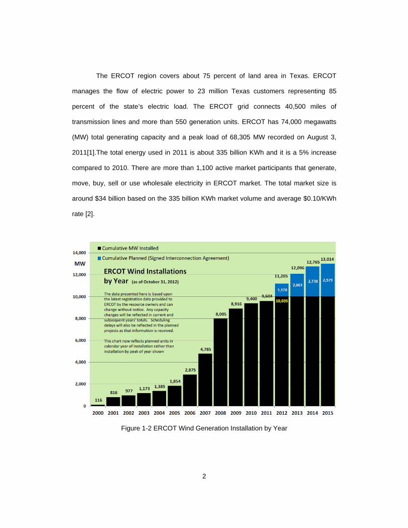
ERCOT’s installed wind generation capacity is the highest among major ISOs in
the United States. The ERCOT wind generation installation by year is shown in Figure
1-2. As of Oct. 31, 2012, ERCOT has 10,035 MW wind generation capacity installed with
nearly 21,000 MW of additional wind generation under review. The wind generation
record is 8,638 MW on Dec. 25, 2012 which accounts for 26 percent of total system load
at the time. On the other hand, because the rapid increase of wind energy and the
intermittence nature of thewind power, it imposes big challenges to system operation.
1.2 ERCOT Nodal Market
In 1999, Senate Bill 7 (SB7) restructured the Texas electricity market by
unbundling the investor-owned utilities and creating retail customer choice in those areas.
areas, and assigned ERCOT four primary responsibilities [2]:
System reliability – planning and operations
Open access to transmission
Retail switching process for customer choice
Wholesale market settlement for electricity production
In 2001, ERCOT began its single control area operation and opened both its
wholesale and retail electricity market to competition based on a zonal market structure.
In the zonal market, the ERCOT region is divided into congestion management zones
(CMZs) which are defined by the commercially significant constraints (CSCs) [2] [4].
In 2003, the Public Utility Commission of Texas (PUCT) ordered ERCOT to
develop a nodal wholesale market design. The redesigned ERCOT grid consists of more
than 4,000 nodes and it will replace the existing CMZs. The implementation of the nodal
market is expected to improve price signals, improve dispatch efficiencies and direct

4
assignment of local congestion [3]-[5]. The changes between the ERCOT zonal and
nodal market are summarized in Figure 1-3 below [3].
Figure 1-3 ERCOT Zonal Market vs. Nodal Market
On Dec. 1, 2010, ERCOT successfully launched the locational marginal pricing
based Nodal Market. The redesigned comprehensive nodal market includes congestion
revenue right (CRR) auction market, a day-ahead market (DAM), reliability unit
commitment (RUC) and real-time security constrained economic dispatch (SCED).
A congestion revenue right (CRR) is a financial instrument that entitles the CRR
owner to be charged or to receive compensation for congestion rents that arise in the
day-ahead market (DAM) or in real-time. Owning a CRR doesn’t provide the CRR owner
a right to receive or obligation to deliver the physical energy. CRRs are defined by a MW
amount, settlement point of injection (source) and settlement point of withdrawal (sink).
There are two types of CRR ownership: point-to-point (PTP) Obligations and point-to-
point (PTP) Options. The PTP Obligation may result in either a payment or a charger for
the CRR ownership but the PTP Options can only result in a payment for the CRR

5
Ownership. CRRs are auctioned by ERCOT monthly and annually and the revenues
collected from the auctions are returned to loads base on the load ratio share.
The day-ahead market (DAM) is a forward financial electricity market cleared in
day-ahead. The DAM clearing process co-optimizes the energy offers and bids, ancillary
services and certain types of congestion revenue rights (CRRs) by maximize system-
wide economic benefits. The DAM clearing results include the unit commitments for
resources with three-part supply offer, the awards for energy offers and bids, awards for
ancillary services and awards for certain type of CRRs. The DAM scheduling also
complies with network security constraint in addition to the usual resource constraints.
The main purposes for the DAM are scheduling energy and ancillary services, providing
price certainty and discovery for the next operating day.
The reliability unit commitment (RUC) is a daily or hourly process conducted to
ensure sufficient generation capacity is committed to reliably serve the forecasted
ERCOT demand [6]. RUC is also used to monitor and ensure the transmission system
security by performing the network security analysis (NSA). The DAM clearing is based
on the voluntary energy offers and bids instead of the load forecast. The resources
committed in the DAM may not be sufficient to meet the actual energy and ancillary
service capacity requirements in real-time. Hence the RUC process is needed to procure
enough resource capacity to meet load forecast in addition to ancillary service capacity
requirement. The RUC process works like a bridge filling the capacity gap between the
financial DAM and real-time to ensure the reliable operation of the ERCOT market. There
are three RUC processes used in the ERCOT nodal market:
Day-ahead RUC (DRUC): DRUC runs once a day. It is used to determine if additional
commitments needed to be made for the next operating day.

6
Hourly RUC (HRUC): HRUC process is executed every hour. It is used to fine-tuning
the commitment decision made by DRUC based on the latest system condition.
Weekly RUC (WRUC): WRUC process is an offline planning tool. Its study period is
configurable and could be up to one week.
During real-time operations, the security constrained economic dispatch (SCED)
dispatches online generation resources based on their Energy Offer Curves to match the
total system demand provided by the EMS while observing resource ramping and
transmission constraints. The SCED process produces the base point and locational
marginal prices (LMPs) for each generating resource. ERCOT uses these base points to
deploy various ancillary services such as regulation up, regulation down, responsive
reserve, and non-spinning reserve services to control system frequency and solve
potential reliability issues [10].
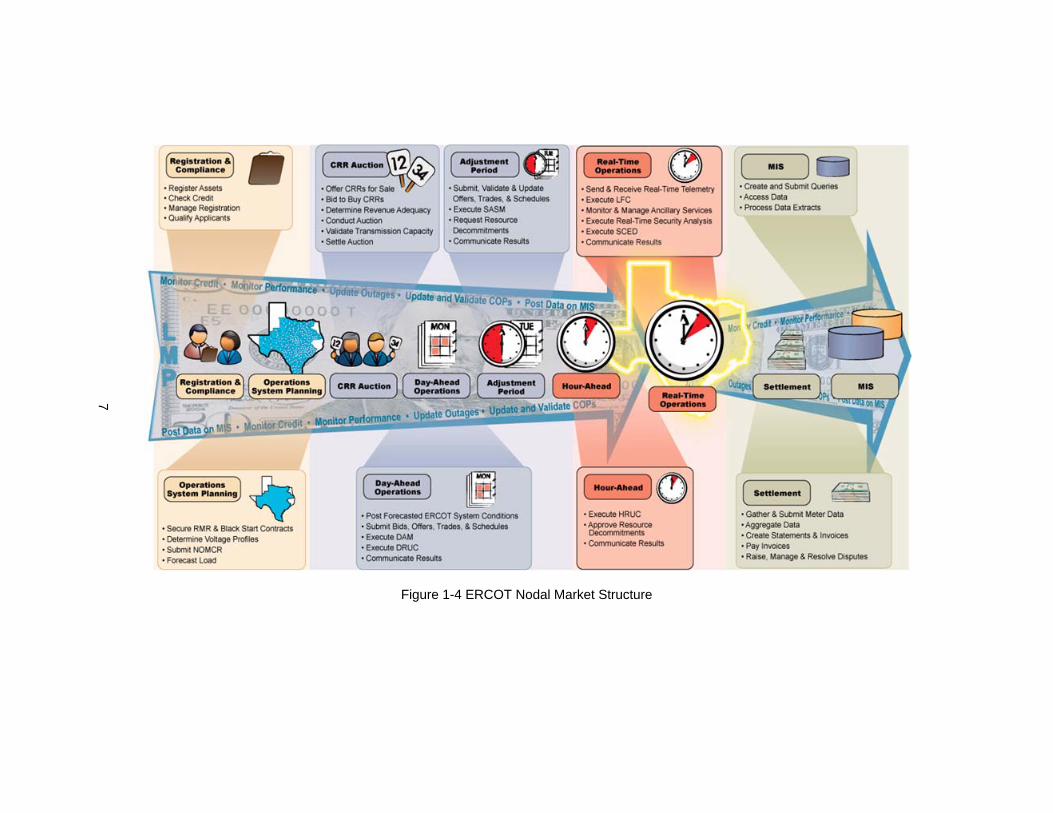
The ERCOT nodal market structure is illustrated in Figure 1-4 [4]. The
adjustment period is defined as the time between 1800 of day-ahead up to the 60
minutes prior to the operating hour. The MIS denotes the market information system
which is an electronic communication interface used by ERCOT to provide information to
the public and market participants.
The two-settlement system [10] has been adopted for the ERCOT nodal market.
The two-settlement provides the ERCOT market participants with the option to participate
in a forward market for energy. It consists of two markets: day-ahead forward market and
real-time balancing market and it separates the settlements performed for each market.
The Day-ahead market settlement is based on the scheduled hourly quantities and day-
ahead hourly LMPs and the real-time market settlement is based on the actual 15-
minutes quantity deviations from the day-ahead schedules priced at real-time LMPs.
7
Figure 1-4 ERCOT Nodal Market Structure

8
1.3 Unit Commitment Review
1.3.1 Introduction
The unit commitment (UC) is the optimization process of determining the startup
and shutdown schedules of generation units over a given study period [7]-[11]. The UC
optimization is extensively used in short term daily system operations for study period
from one to seven operating days and it is also used for operational planning and
portfolio evaluation over longer time horizon.
The security constrained unit commitment (SCUC) is a major enhancement and
extension of the conventional unit commitment [13]-[17]. In SCUC, the security is
explicitly takes into account by ensuring transmission constraints both base case and
post-contingency are within the limits. By incorporating security network constraints, the
generation units are committed economically in a manner to ensure that the system is still
secure for all credible contingencies.
SCUC has already replaced the conventional UC in many major electricity
markets including the North America. In the deregulated electricity market, SCUC is
utilized by ISO/RTO to clear the day-ahead market (DAM) and perform reliability unit
commitment (RUC) [24]-[27]. The objective of SCUC is to minimize system operating
costs while satisfying various system and resource constrains, such as power balance,
system ancillary service requirements, transmission constraints, minimum and maximum
generation limits, minimum up and down time limits, ramping up/down limits, tap position
and limits of phase shifters [13].
With the increased penetration of renewable resources and the increase of
demand response participation, how to model the uncertainty in the ISO SCUC becomes
a big challenge. Recently, stochastic unit commitment [18] [19] [28] and robust unit
commitment [29] have been proposed for uncertainty modeling and risk management.

9
The stochastic unit commitment minimizes the expected cost of the unit commitment
problem. It is a conventional way to model the unit commitment problem with the real-
time uncertainties. The advantage of the stochastic unit commitment is able to quantify
the expectations such as evaluating probability of outcomes and the disadvantages are
computationally challenging and difficulty to decide the exact and accurate distribution.
However it requires the knowledge of probability distribution of the uncertain parameters.
The robust unit commitment minimizes the cost of unit commitment problem for the worst
case. It models the random demand using uncertainty sets instead of probability
distributions. The advantages of the robust unit commitment are computationally tractable
and free of distribution. However, it is unable to provide probability measure such as
expectations and difficulty to choose the right uncertainty set [29]. Both of these two
methods are still in the research phase and haven’t been implemented in the ISO
production system.
1.3.2 Unit Commitment Solution Methodology
The unit commitment problem is a complicated large-scale mixed-integer and
nonlinear optimization problem which has been an active research topic for several
decades. Recent literature review on the unit commitment solved either by the ISO or by
the producers can be found in [47] [48]. As a consequence, various optimization
algorithms such as exhaustive enumeration [49] [50], priority listing [51]-[53], dynamic
programming [54]-[56], Lagrangian relaxation [57]-[65], mixed-integer programing [66]-
[74], simulated annealing [75]-[77], and generic algorithms [78]-[81] have been developed
to solve the optimal UC problem. Among these algorithms, the mixed integer programing
(MIP) and Lagrangian relaxation (LR) are the most widely applied methods among
industry.
10
Until recently, the LR was the primary solution method for the traditional unit
commitment software executed by system operators in control center [24] [27]. However
in the last decade, the advances in computer hardware and the commercial MIP solver
make the MIP as the dominant practical solution to the large ISO size UC problems [24]-
[27]. The comparisons between MIP and LR for the ISO unit commitment problem are
discussed in [24], [82], and [83]. The main advantages of the MIP formulation over the LR
formulation are that 1) it can provide a global optimality, 2) it provides a more accurate
measure of optimality, 3) it improves the security constraints modeling and 4) it provides
enhanced modeling capabilities and adaptability [24] [83]. In addition, the major benefit of
using the MIP in the development is that it allows the developer to focus on the problem
definition itself rather than the optimization algorithm development. It is much simpler to
add new constraints into the MIP formulation without involving heuristic, which will reduce
the software development cycle and facilitate its application to the large UC problem.
Though the main disadvantage for the MIP formulation over LR is its scalability and run
time [25], [68], and [69], the commercial MIP solvers are capable of solving the ISO size
SCUC problem within acceptable time. The MIP formulation becomes the recent trend for
the large and complex ISO SCUC problems including both day-ahead market clearing
and reliability unit commitment.
Once the SCUC problem is formulated and represented in the MIP format, the
solution can be sought by calling a standard MIP package such as CPLEX [84], GUROBI
[85], LINDO [86], Xpress [87], and so on. Among of these MIP packages, the commercial
CPLEX solver is well known for its high performance and it is robust and reliable. The
CPLEX’s mathematical programming technology enables analytical decision support for
improving efficiency, reducing costs, and increasing profitability [84]. Hence the
CPLEX/MIP has been widely utilized by the ISO to solve the SCUC problem.

11
1.4 Reliability Unit Commitment in ERCOT Zonal Market
The zonal market of ERCOT is based on the transfer capacity of the 345KV
transmission network between CMZs. The CMZs are determined by clustering load and
generator buses based on their shift factors on selected Commercially Significant
Constraints (CSCs). In order to facilitate the zonal operations, transmission constraints
are categorized into intra-zonal (local) and inter-zonal constraints.
In zonal market, the replacement reserve service (RPRS) performs similar
functions as the RUC in the nodal market [20][30]. The RPRS market is run at the day-
ahead and during the adjustment period if needed to procure additional capacity from
specific generation or load resources to resolve system capacity insufficiency, inter-zonal
and intra-zonal congestion. Required by ERCOT zonal protocols, the cost associated
with the procurement of RPRS for capacity insufficiency and inter-zonal congestion are
directly assigned to those market participants who have negatively impacted the system.
The costs for intra-zonal congestion are uplifted to all loads in the ERCOT system. To
distinguish between procured resources for relieving intra-zonal constraints versus inter-
zonal and system capacity constraints, the clearing of the RPRS market employs a 3-
step process:
Step 1 procures capacity to resolve intra-zonal congestion using the resource
category generic costs.
Step 2 procures capacity to resolve inter-zonal congestion and system capacity
constraints using market-based offers.
Step 3 determines the RPRS market clearing prices for capacity.
The RPRS process has been officially online since early 2006 and it has greatly
helped ERCOT operators to make the reliability commitment decisions. However the
following challenges and deficiencies for the RPRS have also been identified by ERCOT:

12
Due to the multi-step congestion relief process, there is no guarantee that the intra-
zonal congestion will remain secure after the step2 procurement.
The RPRS does not model the resource specific ancillary service (AS) schedules in
the clearing. The ancillary schedules are submitted by Qualified Scheduling Entities
(QSEs) on a portfolio basis and the RPRS only enforces a system capacity constraint
for the system total online AS requirements. This approach cannot identify the AS
deliverability problems and it may cause the RPRS under procurement problem.
There are deficiencies in handling the scheduling of some special resources in
RPRS. For instance, combined cycle resources are modeled the same as individual
physical units. Therefore, the possibility of procuring a steam unit without the
corresponding gas-turbine unit exists. If this situation occurs, ERCOT operators need
to either manually deselect the resource or bring on the additional resources
necessary to create feasible combined cycle configurations.
The above RPRS challenges and deficiencies have been considered during the
nodal RUC design and most of them have been solved in the nodal RUC [6], [30]-[32].
1.5 Objectives of Dissertation
It has been widely accepted that the reliability unit commitment (RUC) process is
required in the restructured electricity markets to maintain system reliability while
minimizing the overall operational cost for committing additional units [20]-[23]. The RUC
function has been implemented in many ISOs, such as PJM, NYISO, MISO, CASIO, and
ISO-NE [23]-[27]. Unlike the day-ahead market (DAM) which provides a financial platform
for market participants to trade energy, RUC is critical to power system security in such a
way that it ensures sufficient online resource capacity is available at the right location to
satisfy the demand in real-time. The RUC process utilizes the security constrained unit

13
commitment (SCUC) framework with a full network model to enforce transmission flows
and bus voltages within limit and to meet the (N-1) system reliability criteria. On the other
hand, there are also some technical challenges and issues related to the RUC, such as
combined cycle units modeling, wind modeling [20]-[22].
In ERCOT nodal market, the reliability unit commitment (RUC) process is needed
to determine the commitment of additional offline available resources as necessary on
top of those already self-committed for bilateral contracts and committed by other
markets such as DAM, to meet the forecasted real-time demand plus the ancillary
services (AS) capacity and meet the system's security requirements. The objectives of
this dissertation is to develop a reliability unit commitment (RUC) system to improve the
reliability and efficiency operation of ERCOT nodal market by addressing the issues and
deficiencies observed in the zonal replacement reserve service (RPRS) market.
In this dissertation, the RUC is implemented in a security constrained unit
commitment (SCUC) framework to minimize the total operation costs based on generator
three-part supply offers subject to various system and resource security constraints. The
NCUC-NSM iteration clearing process is applied to solve the SCUC problem. Some
enhanced features are implemented in the SCUC to handle special resource scheduling
such as combined cycle resources, split generation resources and self-committed
resources. The mixed integer programming (MIP) methodology has been adopted to
solve the SCUC problem.
The combined cycle unit is modeled in two different ways in SCUC. The
configuration-based model is more adequate for bid/offer processing and dispatch
scheduling and therefore it is adopted in the NCUC. On the other hand, the physical unit
modeling is more adequate for the power flow and network security analysis and
therefore it is adopted in the NSM.

14
The phase shifters installed in ERCOT are primarily for relieving transmission
overloads caused by variations in wind generation. To improve dispatch efficiency and
accuracy, a phase shifter optimization model has been proposed to automatically
determine the tap positions of the phase shifters in the RUC optimization algorithm.
The proposed RUC system has been successfully implemented in the ERCOT
production system. The results show that the proposed RUC system is very robust and
can improve dispatch efficiency and ensure more effective congestion management.
1.6 Organization of the Dissertation
This dissertation consists of seven chapters and two appendixes. The contents of
this dissertation are organized as follows.
Chapter 1 first presents the overview of ERCOT and its recently redesigned
nodal market. Next it reviews the unit commitment problem and the associated solution
methodologies. Then it discusses the issues with replacement reserve service (RPRS) in
zonal market, last it discusses the objectives of the dissertation as well as the
organization of this dissertation.
Chapter 2 first introduces the new RUC process under the new ERCOT nodal
market design. Next it discusses the RUC input and pre-processing, then it discusses
some special scheduling features of the RUC system. Last it presents the settlement of
the nodal RUC process.
Chapter 3 discusses the proposed RUC solution engine implemented in the
framework of security constrained unit commitment (SCUC). First, it presents the two
main functional components of the SCUC: network constrained unit commitment (NCUC)
and network security monitor (NSM). Next, it presents the proposed NCUC-NSM iterative
clearing process for the RUC process.

15
Chapter 4 first reviews various ways of modeling of combined cycle resources in
the literatures. Next it discusses the proposed combined cycle unit scheduling modeling
for RUC.
Chapter 5 first introduces the wind integration in ERCOT and next it discusses
the wind generation scheduling and the proposed phase shifter optimization in RUC.
Chapter 6 presents the test systems and case studies with the proposed RUC
system. First, the author developed prototype RUC program is tested on a 5-bus test
system with several test cases to illustrate the scheduling features especially the
combined cycle resource scheduling. After that, the results of the production RUC
software running on the ERCOT production system are discussed.
Chapter 7 summarizes the conclusion and contribution of this work. The
dissertation concludes with the suggestions for future research.
Appendix A presents the notation used throughout the dissertation.
Appendix B presents the acronyms used throughout in the dissertation.

16
Chapter 2
Reliability Unit Commitment Process in Nodal Market
2.1 Reliability Unit Commitment Process
In the ERCOT nodal market, RUC is an important process to assess the need to
commit generation capacity by evaluating the detailed network model instead of using
simplified zones. The network model used in nodal market consists of more than 4000
nodes and all transmission lines greater than 60 KV. The main objective of RUC process
is to recommend commitment of generation resources to ensure that enough capacity is
committed in the right locations for reliable operation of the ERCOT market.
RUC commits additional generation capacity on top of the self-committed
capacity projected by the current operating plans (COPs) submitted by the QSEs to meet
the forecasted demand subject to transmission constraints and resource characteristics.
As shown in Figure 2-1, there are three RUC processes used in the ERCOT nodal
market [5] [6]:
Day-Ahead RUC (DRUC): The DRUC process is executed daily at 1430 of the day-
ahead after the close of the DAM. The DRUC study period covers the next operating
day. The time step for each RUC interval is one hour. DRUC uses three-part supply
offers that were considered but not awarded in the DAM.
Hourly RUC (HRUC): The HRUC process is executed every hour. The HRUC study
period is either (1) the balance of the current operating day, if the DRUC process has
not been solved, or (2) the balance of the current operating day plus the next
operating day, if the DRUC process has been solved. HRUC is used to fine-tune the
resource commitments using the most updated load forecasts and outage
information. HRUC is also used to approve or reject resource self-decommitment
requests during the adjustment period.

17
Weekly RUC (WRUC): The WRUC process is a look-ahead planning tool. Its study
period is configurable and it could be up to one week. WRUC is used to help ERCOT
manage generation resources that have startup times longer than the DRUC or
HRUC study periods. The WRUC doesn’t send commitment instruction to the QSE.
Figure 2-1 RUC Timeline Summary

18
It is also possible for the RUC processes to decommit self-committed generation
resources; however, this will happen only if the decommitment is necessary to resolve
transmission congestion that is otherwise irresolvable.
In addition to the dispatch instructions to notify each QSE of its resource
commitment schedules, RUC also makes the following market information available:
All binding and violated transmission constraints detected by RUC algorithm.
All resources committed or decommitted by the RUC process.
2.2 RUC Input Data
The RUC input and initialization module retrieves various input data from
interfaces of different external systems and prepares it for use by the market clearing
module. The detail of the major input data is discussed as follows.
a) Current Operating Plan (COP)
The COP is an hourly plan submitted by a QSE reflecting anticipated operating
conditions for each of the resources that it represents for each hour in the next seven
operating days. The COP includes the following data:
Resource name.
The expected resource status: The operational state of a resource, e.g. ON-online,
OFF-offline and available for commitment, OUT-offline and unavailable.
High sustained limit (HSL): The maximum sustained energy production capability for
a resource established by the QSE.
Low sustained limit (LSL): The minimum sustained energy production capability for a
resource established by the QSE. A resource’s dispatch MW needs to be between
LSL and HSL to respect the physical limit.
Ancillary service resource responsibility capacity in MW for

19
o Regulation up service (Reg-Up)
o Regulation down service (Reg-Dn)
o Responsive reserve service (RRS)
o Non-Spinning reserve service (Non-Spin)
The high ancillary service limit (HASL) and low ancillary service limit (LASL) are
dynamically calculated MW upper and low limit on a resource to reserve the part of the
resource’s capacity committed for Ancillary Service. The formula for the HASL and LASL
calculation is shown below:
HASL = Max (LASL, HSL – Reg-Up – RRS - Non-Spin)
LASL = LSL + Reg-Dn
It should be noted that for combined cycle train (CCT) including multiple
configurations, the QSE shall submit the COP for each operating configuration. For split
generation resource (SGR), the QSE shall submit the COP for each logical SGR. One
example of the COP for resource ALTA is shown in Table 2-1.
Table 2-1 An Example of COP
Resource Name
Operating Day
Hour Ending
Resource Status
LSL(MW)
HSL(MW)
Reg-Up(MW)
Reg-Dn(MW)
RRS (MW)
Non-Spin(MW)
ALTA 12/01/2012 1 OUT 11 110 0 0 0 0
ALTA 12/01/2012 2 OUT 11 110 0 0 0 0
ALTA 12/01/2012 3 OFF 11 110 0 0 0 0
ALTA 12/01/2012 4 OFF 11 110 0 0 0 0
… … … … … … … … … …
ALTA 12/01/2012 15 ON 11 110 5 10 20 30
ALTA 12/01/2012 16 ON 11 110 10 5 10 20
ALTA 12/01/2012 17 ON 11 110 0 0 0 0
ALTA 12/01/2012 18 ON 11 110 0 0 10 0
… … … … … … … … … …
ALTA 12/01/2012 24 OFF 11 110 0 0 0 0

20
b) Three-Part Supply Offer
The three-part supply offer is an hourly offer submitted by a QSE for a generation
resource that it represents for each hour. The three-part supply offer contains three
components: (1) startup offer for each cold, intermediate and hot condition, (2) a
minimum-energy offer and (3) an energy offer curve. The energy offer curve is piece-wise
linear non-decreasing curve and can be up to 10 price/quantity break points. Table 2-2
illustrates an example of the three-part supply offer.
Table 2-2 An Example of Three-Part Supply Offer
c) Mitigated Offer Cap Curve
The mitigated offer cap curve is used to cap the energy offer curves in real-time
operations. The mitigated offer cap curve is calculated non-decreasing offer based on
resource specific verifiable cost if available or based on the generic value. Similar to the
three-part supply offer, the mitigated offer cap can be up to 10 price/quantity break
points. One example is shown in Figure 2-2.
Hot Inter Cold Q1 P1 Q2 P2 Q3 P3 Q4 P4 Q5 P5 … … Q10 P10
ALTA 12/01/2012 1 1000 1200 1400 20 0 14 110 14
ALTA 12/01/2012 2 1100 1300 1500 20 0 10 11 10 50 15 80 20 110 25
ALTA 12/01/2012 3 1000 1000 1000 25 0 12 11 12 30 15 60 18 80 20 … … 110 30
ALTA 12/01/2012 4 1100 1300 1500 25 0 14 11 14 20 15 30 20 50 30 … … 110 40
… … … … … … … … … … … … … … … … … … … … …
ALTA 12/01/2012 24 1100 1300 1500 25 0 14 11 14 20 15 30 20 50 30 … … 110 40
ResourceName
Startup Offer ($) MEO($/MWh)
OperatingDay
HourEnding
Energy Offer Curve (Q-MW, P-$/MWh)

21
Quantity (MW)
Mitigated Offer Cap
($/MWh)
Figure 2-2 An Example of Mitigated Offer Cap Curve
d) Verifiable Cost
The RUC retrieves the resource specific verifiable cost from settlement system.
The verifiable startup and minimum-generation cost are used to create offers for non-
offer resources in RUC. The verifiable incremental energy cost is used to calculate the
mitigated offer cap curve.
e) Resource Parameters
The RUC retrieves the following resource parameters submitted by the resource
entity from registration system:
Resource name.
Resource type: steam turbine, hydro, gas turbine, combined cycle etc.
Qualifying facility (QF) Status: A qualifying small power production facility or
qualifying cogeneration facility under certain regulatory qualification criteria.
Minimum online time: The minimum number of consecutive hours that the resource
must be online before it can be shut down.

22
Minimum offline time: The minimum number of consecutive hours the resource must
be offline before it can be restarted.
Normal ramp rate curve: It is a staircase curve submitted by the QSE and can be up
to ten segments. Each segment indicates the rate of change in MW per minute of a
resource within the corresponding output MW range.
Emergency ramp rate curve: It is a staircase curve submitted by the QSE and can be
up to ten segments. Each segment indicates the maximum rate of change in MW per
minute of a resource within the corresponding output MW range to provide
responsive reserve (RRS) deployed by ERCOT.
Start time in hot, intermediate and cold temperature state: the stat time a.k.a. lead
time specifies the number of hours from the ERCOT notice time (i.e. the time
generators are notified of the commitment by ERCOT) to the time the generator can
be started up in the corresponding temperature state. The start time is a function of
the generator offline time.
Maximum online time: The maximum number of consecutive hours a resource can be
online before it needs to be shut down.
Maximum daily starts: The maximum number of times a resource can be started up in
an operating day under normal operating conditions.
Hot-to-Intermediate Time: The number of hours that a resource after shutdown takes
to cool down from hot temperature state to intermediate temperature state.
Intermediate-to-Cold Time: The number of hours that a resource after shutdown
takes to cool down from intermediate temperature state to cold temperature state.
Maximum weekly starts: The maximum number of times a resource can be started up
in seven consecutive days under normal operating conditions.

23
Maximum weekly energy: The maximum energy in MWh a resource can produce in
seven consecutive days.
Besides the resource parameters for regular resources, the combined cycle
resources have additional resource parameters and they will be discussed in detail in
Chapter 4.
f) Transmission Outage Data
The RUC retrieves the transmission outage information from outage scheduler
(OS) and use the outage information to build the network topology.
g) Dynamic Rating from EMS
The RUC retrieves dynamic ratings data from the EMS for transmission
equipment where available. The dynamic rating is used in network security monitor
(NSM) function. The RUC uses default static ratings data from the EMS for the
transmission equipment which don’t have dynamic ratings data available. The dynamic
ratings are weather-adjusted MVA limits for each hour of the study period for all
transmission lines and transformers. There are three types of dynamic ratings:
Normal rating: Normal rating is the rating at which a transmission element can
operate without reducing its normal life expectancy. The normal ratings are enforced
in NSM base case power flow study.
Emergency rating: Emergency rating is the 2-hour rating of a transmission element.
The emergency ratings are enforced in NSM during the post-contingency analysis.
15-minute rating: 15-minute ratings are short-term ratings of a transmission element.
NSM will issue warnings if any of the 15-minute ratings are violated.
h) Generic Constraints from EMS
The generic constraints are the network/voltage constraints modeled as
import/export energy constraints that are determined offline.

24
i) Load Forecast from EMS
The RUC retrieves the most current hourly load forecast from mid-term load
forecast (MTLF) application from EMS for each weather zone. The MTLF predicts the
hourly loads for the next 168 hours based on current weather forecast parameters within
each weather zone. The accuracy of the load forecast is critical to the RUC since it is
used by RUC to secure generation capacity
The MTLF has a self-training mode and is updated every hour for the next 168
hours. The following inputs are used by the MTLF [5]:
Hourly forecasted weather parameters for the weather stations within the weather
zones, which are updated at least once per hour; and
Training information based on historic hourly integrated weather zone loads.
The ERCOT System-wide Load Forecast is calculated as the sum of load
forecasts for all the weather zones. The network losses are already included in the load
forecast that is considered in RUC processes.
j) Current and Historical Resource Commitment Status from EMS
The RUC retrieves both the current resource commitment status and historical
resource commitment status of the current operating day from the EMS. The current
commitment status indicates if the resource is online or offline at current time. The
historical commitment status includes the following information:
Number of startups in current operating day until the end of previous hour.
Online hours at the end of previous hour since last status change.
Offline hours at the end of previous hour since last status change.
It should be noted that the online hours and offline hours above are mutually
exclusive. If the last status change is startup, i.e. from offline to online, the online hours is
greater than 0 and the offline hours is 0. If the last status change is shutdown, i.e. from

25
online to offline, the online hours is 0 and offline hours is greater than 0. Based on the
historical commitment status, the RUC can determine the time when the resource
changed status to online/offline.
k) Load Distribution Factors from EMS
The RUC retrieves the hourly load distribution factors (LDF) from EMS for each
hour in the study period. Each load can be mapped to a specific electrical bus and a
specific weather zone. Each load is classified as either conforming or non-conforming but
not both. The LDF is used for bus load forecast.
l) Current Breaker and Switch Status from EMS
The HRUC retrieves the current breaker and switch status from SCADA/EMS
and uses it plus changes indicated in Outage Scheduler to build network topology for the
first study hour.
2.3 RUC Initialization and Pre-processing
2.3.1 Proxy Energy Offer Curve Creation
The RUC calculates proxy energy offer curves for all resources based on their
mitigated offer caps to substitute their original energy offer curves. The calculated proxy
energy offer curves will then be used by the RUC market clearing engine to determine
the projected energy output level of each resource and to project potential congestion
patterns for each hour of the RUC.
The RUC calculates the proxy energy offer curves by multiplying the mitigated
offer cap by a configurable discount parameter and applying the cost for all generation
resource output between high sustained limit (HSL) and low sustained limit (LSL).
The proxy energy offer curve is calculated in a way that discounts the
incremental energy cost to ensure the self-committed online resources are used to the

26
fullest extent before additional RUC commitment. This approach will minimize the out of
market reliability commitment which may over mitigate the competitive market price. In
turn, this approach will also minimize the RUC “make-whole” payment resulting from the
startup and minimum-energy cost.
2.3.2 Modeling Resource Capacity Providing Ancillary Service
The RUC treats all resource capacity providing ancillary service (AS) as
unavailable for the RUC study period, unless that treatment leads to infeasibility (i.e., that
capacity is needed to resolve some local transmission problem that cannot be resolved
by any other means). In such cases, the RUC will provide the information for each
affected QSE of the amount of its resource capacity the projected hours that does not
qualify to provide AS.
The following approach has been proposed to protect the ancillary service
capacity. After the RUC creates the proxy energy offer curve for a resource, it modifies
the proxy energy offer curve to protect the capacity providing ancillary services. First the
RUC calculates Resources’ HASL and LASL based on the HSL, LSL, and ancillary
service quantities from COP. Then the RUC modifies the portions of resource proxy
energy offer curve outside HASL and LASL by assigning penalty factors for the
corresponding ancillary services. The penalty factors are higher than any of the proxy
energy offer curves but lower than transmission constraint penalty factor. The penalty
factors for resource AS violation and transmission constraint violation are configurable
parameters and can be adjusted by authorized users.
Figure 2-3 illustrates the proxy energy offer curve with ancillary services
protection. As shown in the figure, the capacity providing regulation down service (Reg-
Dn) will be assigned a negative penalty factor. The capacities providing regulation up
service (Reg-Up), responsive reserve (RRS), and non-spinning reserve (Non-Spin) is
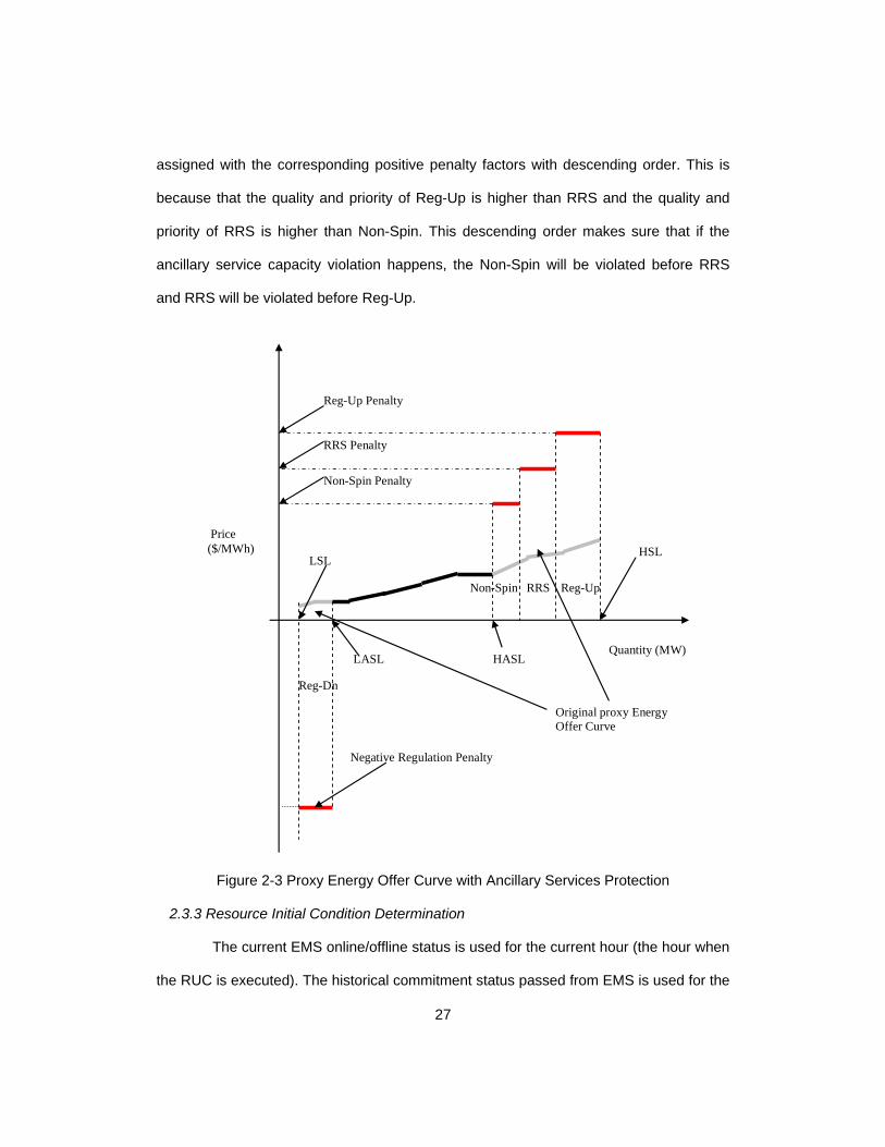
27
assigned with the corresponding positive penalty factors with descending order. This is
because that the quality and priority of Reg-Up is higher than RRS and the quality and
priority of RRS is higher than Non-Spin. This descending order makes sure that if the
ancillary service capacity violation happens, the Non-Spin will be violated before RRS
and RRS will be violated before Reg-Up.
Original proxy Energy Offer Curve
Quantity (MW)
Reg-Up Penalty
RRS Penalty
Non-Spin Penalty
Negative Regulation Penalty
Price ($/MWh)
Non-Spin RRS Reg-Up
Reg-Dn
HASL LASL
LSL HSL
Figure 2-3 Proxy Energy Offer Curve with Ancillary Services Protection
2.3.3 Resource Initial Condition Determination
The current EMS online/offline status is used for the current hour (the hour when
the RUC is executed). The historical commitment status passed from EMS is used for the

28
status before the current hour. For future hours, the commitment status indicated in the
COP is used. Due to the difference of the study period, the following rules are applied for
different RUC processes:
The DRUC and WRUC uses the historical commitment data, the online and offline
status for the current operating hour and the COP status for remaining hours of the
current operating day to project the initial commitment status at the beginning of the
next operating day.
The HRUC uses the historical commitment data and the online and offline status for
the current operating hour to determine the resource’s initial condition at the
beginning of the next operating hour.
If the COP is not available for any resource for any particular hour from the
current hour to the start of the RUC study then the resource status for those hours are
considered as equal to that of the last known hour’s COP for that resource.
It is expected that at most one configuration of the same combined cycle train
(CCT) will have online COP status for any hour. However, in practice, it may occur that
the same CCT has more than one configuration having online COP status for the same
hour. In this case, for any hour before the RUC study period, the online configuration
which has been online for the longest time is considered as online and all the other online
configurations from the same CCT will be treated as offline.
If a resource is offline between the RUC execution and the beginning of the study
period, the start time of the resource can affect its eligibility to be committed. The
following logic has been proposed and implemented to enforce the start time constraint:
First, the RUC determines the resource temperature state (hot/intermediate/cold) at
the RUC execution based on the resource’s historical offline time and hot-to-
intermediate and intermediate-to-cold cooling time.

29
Second, the RUC determines the start time corresponding to the temperature state
Third, the RUC makes the resource unavailable for commitment from the current time
to the start available time min (current time + configurable offset + start time, first
hour resource scheduled online in the COP). Where the configurable offset is the
delay time from the RUC execution time to the RUC notice of commitment to the
resource, i.e. the RUC execution time.
Use DRUC as an example. Assume DRUC is executed at 1430 at current
operating day with the study period as the next operating day. The configurable offset is
set as 15 minutes. Resource ALTA has been offline for 14 hours based on its EMS
historical commitment status and the COP status is also offline from HE15 of current
operating day to HE24 of next operating day. The hot-to-intermediate time is 6 hour and
the intermediate-to-cold time is 3 hour. The hot, intermediate and cold start time is 3, 6
and 12 hour respectively. Since the offline time (14 hours) is greater than hot-to-cold time
(6+3=9 hours), the resource ALTA is in cold status at 1430. So the cold start time (12
hour) is used as the corresponding start time. Define OD is current operating day and
OD+1 is next operating day. So the start available time is calculated as min(OD 1430
+1/4 hour+12 hours, OD+1 2400)=OD+1 0245. The RUC will set the resource ALTA as
unavailable from HE1 to HE3 to observe the start time.
2.3.4 Bus Load Forecast
The RUC needs to determine a forecast of the load at each electrical bus for
each hour in the study period before performing the network security analysis including
both base case power flow and contingency analysis. The following steps are used in the
bus load forecast:

30
First, RUC identifies the non-conforming loads, allocates the MW schedules from the
load distribution factor (LDF) for non-conforming loads to the mapping electrical
buses directly and subtracts them from the weather zone load forecast.
Second, RUC distributes the remaining weather zone load forecast to the conforming
loads based on their LDF.
Last, RUC identifies all the isolated loads and performs load rollover based on the
load rollover definition if any.
2.3.5 DC Ties Modeling
Currently there are five DC Ties interconnected to ERCOT system. The location
and capacity is shown in Figure 2-4. The Laredo DC Tie (DC_L) is a 100 MW variable
frequency transformer located at the AEP Laredo VFT station and connects the ERCOT
Region with CFE in Mexico, even though this interface is not a back-to-back HVDC
converter, it is used as a DC Tie.
The following logic has been proposed and implemented for the DC Ties
modeling in the RUC:
Retrieve 15-minute DC Tie energy schedules from NERC eTag and aggregate to
hour level for each DC Tie.
Each DC Tie is modeled as an equivalent generator resource if the net energy
schedule for the DC Tie shows a net import, otherwise it is modeled as an equivalent
load resource.
RUC treat the net DC Tie schedule as a fixed injection (import) or withdraw (export)
in the network security analysis.
RUC calculates the system total net DC Tie schedules by summing up the net DC Tie
schedule across all the DC Ties for the same hour.
RUC calculates the net system load to be served by ERCOT generation by

31
o Subtracting the net system total DC Tie schedule from load forecast if the net
schedule is import.
o Adding the net system total DC Tie schedule to load forecast if the net schedule
is export.
Figure 2-4 ERCOT DC Ties Location and Capacity
2.4 RUC Special Scheduling Features
2.4.1 Split Generation Resources
A split generation resource (SGR), a.k.a. a jointly owned unit (JOU), is a
generation resource that has been split to function as two or more independent
generation resources represented by different market participants. The individual SGR is
32
treated as a logical resource in RUC and it can participate in the ERCOT nodal market
the same as regular resources. Each individual SGR has a distinct full set of resource
operation parameters and market submissions such as three-part supply offers and COP
schedules. Due to the physical operational constraint, the individual SGRs in a
generation facility must be committed or decommitted together by NCUC. For network
security analysis, all the individual SGRs in a generation facility are treated as a single
physical resource in NSM. The dispatch from individual SGRs is aggregated on a
physical resource basis prior to being sent to NSM for evaluation. In turn, the NSM
provides shift factors for the individual SGRs to NCUC. Note that the shift factors are
identical since the individual SGRs belongs to a same physical resource.
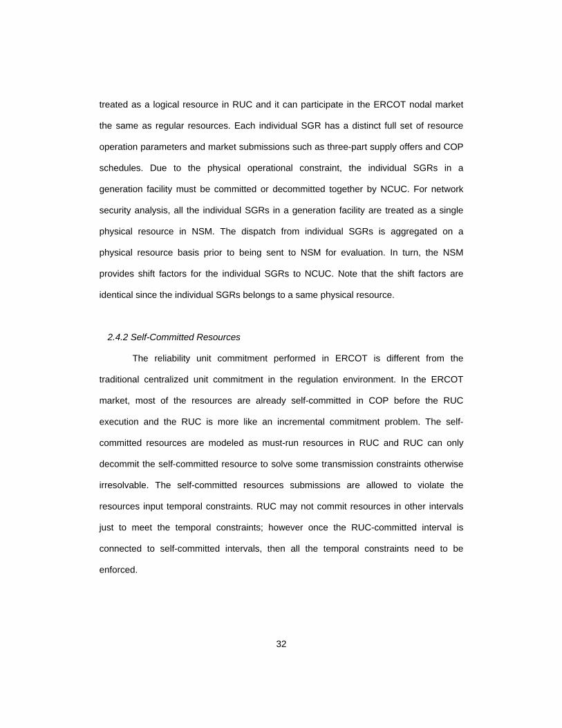
2.4.2 Self-Committed Resources
The reliability unit commitment performed in ERCOT is different from the
traditional centralized unit commitment in the regulation environment. In the ERCOT
market, most of the resources are already self-committed in COP before the RUC
execution and the RUC is more like an incremental commitment problem. The self-
committed resources are modeled as must-run resources in RUC and RUC can only
decommit the self-committed resource to solve some transmission constraints otherwise
irresolvable. The self-committed resources submissions are allowed to violate the
resources input temporal constraints. RUC may not commit resources in other intervals
just to meet the temporal constraints; however once the RUC-committed interval is
connected to self-committed intervals, then all the temporal constraints need to be
enforced.

33
2.4.3 RUC Startup Cost Eligibility
For the purpose of evaluating a resource’s startup cost eligibility, all contiguous
RUC-committed hours are considered as one RUC instruction. For each resource, only
one startup cost is eligible per block of contiguous RUC-committed hours. Based on the
nodal protocol [5], the startup cost for the contiguous RUC-commitment block may not be
eligible to be included in the RUC make-whole payment if the designated start hour or
last hour of the RUC instruction connects to a block of QSE-committed intervals that was
QSE-committed before the RUC instruction was given. For example, consider the case
where the QSE self-committed intervals are from HE1 to HE6 and all the other intervals
are offline. If RUC commits interval from HE7 to HE12, which connects QSE-committed
intervals, the startup at interval HE7 is not eligible for startup cost.
The startup cost modeling in optimization reflects the above settlement rules. The
RUC NCUC optimization doesn’t introduce additional resource startup cost in the
objective function if RUC-committed hours connect to the QSE self-committed intervals.
2.4.4 SPS/RAP Modeling
A special protection system (SPS) or remedial action plan (RAP) is a set of
automatic or pre-defined actions taken to relieve transmission security violations during
the post-contingency condition. These SPSs and RAPs are sufficiently dependable to
assume that they can be executed without loss of reliability to the ERCOT network. The
SPSs and RAPs will be used for contingency analysis before considering a resource
commitment and this logic will reduce the RUC over procurement.
NSM models all approved special protection systems (SPSs) and remedial action
plans (RAPs) while performing the contingency analysis.

34
2.4.5 Mandatory Participation
The RUC commitment is physically binding and the resources committed by RUC
are required to be online in real-time. The participation in RUC is mandatory for all
available resources regardless of whether they are offered into RUC. Not submitting a
startup offer and a minimum-energy offer does not prevent a resource from being
committed in the RUC process. RUC will create three-part supply offers for all resources
that did not submit a three-part supply offer but are specified in an offline available status
in COP. For such non-offer resources, RUC process uses 150% of any approved
resource specific verifiable startup cost and minimum-energy cost while determining the
commitment schedule. If the verifiable costs have not been approved, RUC will use the
applicable resource category generic startup offer cost and minimum-energy offer cost
instead. However, during the settlement process, for such resources, only 100% of the
approved verifiable or generic startup costs and minimum-energy cost are applied. This
approach is intended to commit the resources with three-part supply offers before
considering the non-offer resources. In turn, it will encourage resources to submit three-
part supply offers into RUC if the resources want to be committed by RUC.
2.5 Settlement of RUC
The “make-whole” payment mechanism [5] [10] is employed by ERCOT for RUC
settlement to make up the difference when the revenues that a RUC-committed resource
receives are less than its operation costs. In general, the RUC settlement consists of the
following three categories:
RUC make-whole payment and charge.
RUC clawback charge and payment.
RUC decommitment payment and charge.

35
A. RUC Make-Whole Payment and Charge
For each RUC-committed resource, RUC settlement calculates the RUC
guarantee which is the sum of the resource’s eligible startup costs and minimum-energy
costs during all RUC-committed hours. If the energy revenues that a RUC-committed
resource receives during RUC-committed hours and QSE clawback intervals are less
than the RUC guarantee, ERCOT will pay the resource RUC make-whole payment for
that operating day to make up the difference.
ERCOT calculates RUC capacity-short charge to charge QSEs whose capacity
are found short and caused the need for RUC commitment. If revenues from the RUC
capacity-short charge are not enough to cover all RUC make-whole payments, ERCOT
calculates the RUC make-whole uplift charge and the difference is uplifted to all QSEs
based on a load ratio share basis.
B. RUC Clawback Charge and Payment
For each RUC-committed resource, if the RUC guarantee is less than the sum of
the energy revenue, ERCOT charges the resource a RUC clawback charge for the
operating day. The clawback rule encourages the QSE to self-commit resources to avoid
high clawback charges and to participate in the day-ahead market. ERCOT uses a higher
clawback percentage for resources that don’t submit three-part supply offers in the day-
ahead market than the ones that submitted three-part supply offers. ERCOT pays the
revenues from all RUC clawback charges to all QSEs, on a load ratio share basis.
C. RUC Decommitment Payment and Charge
If the RUC decommit a QSE self-committed resource that is not scheduled to
shut down within the operating day, then ERCOT pays the affected QSE an amount as a
RUC decommitment payment. ERCOT charges each QSE a RUC decommitment charge,
on a load ratio share basis.

36
Chapter 3
Reliability Unit Commitment Solution Engine
The security constrained unit commitment (SCUC) program is the core solution
engine used by RUC to determine the optimum commitment schedules [6][13][30]. The
SCUC engine is comprised of two major functional components:
Network Constrained Unit Commitment (NCUC) and
Network Security Monitor (NSM).
3.1 Network Constrained Unit Commitment (NCUC)
3.1.1 Introduction
The NCUC function is used to determine projected commitment schedules that
minimize the total operation costs over the RUC study period while meeting forecast
demand subject to transmission constraints and resource constraints. These resource
constraints represent the physical and security limits on resources:
High Sustained Limit (HSL) and Low Sustained Limit (LSL)
Minimum online time
Maximum online time
Minimum offline time
Maximum daily startup
Startup time
The objective function of the NCUC is defined as the sum of startup cost,
minimum-energy cost and incremental energy cost based on three-part supply offers
while substituting a proxy energy offer curve for the energy offer curve. The NCUC also
employs the penalty factors on violation of security constraints in the objective function to
ensure a feasible solution.

37
The proxy energy cost curve is used in NCUC to determine the projected energy
output level of each resource and to project potential congestion patterns for each hour of
the RUC study period. However the dispatch pattern determined by NCUC is only used
by NSM to perform network security analysis and it will not be sent to QSE for generator
dispatch.
The NCUC treats all resource capacity providing ancillary services as unavailable
by enforcing high penalty factors for resource specific ancillary service capacity. If the AS
capacity from the specified resource is needed to resolve some local transmission
congestion that cannot be resolved by any other means, the ancillary service capacity will
be relaxed to resolve the infeasibility.
Normally the NCUC is executed several times iterating with NSM within the
SCUC solution process. The first NCUC run is referred as the initial unit commitment
(IUC). IUC has the same functionality as NCUC except that the network constraints are
not considered. In the remaining NCUC executions, the network constraint data is
prepared by the NSM. The network constraint data is then passed to the NCUC as
additional constraints for enforcement in the optimization process.
3.1.2 Offline Time Dependent Startup Cost Modeling
The NCUC models the offline time dependent startup costs. In the generator
three-part supply offers discussed in Chapter 2, QSE can specify different startup offers
for hot, intermediate and cold temperature state. Correspondingly the startup cost is
modeled as a staircase function of the calculated offline time up to 3 segments, i.e. hot,
intermediate and cold state. An illustration of the staircase startup cost function is shown
in Figure 3-1. The NCUC optimization determines which startup cost will be used based
on the startup cost function.
Conceptually the startup cost is determined based on the following logic
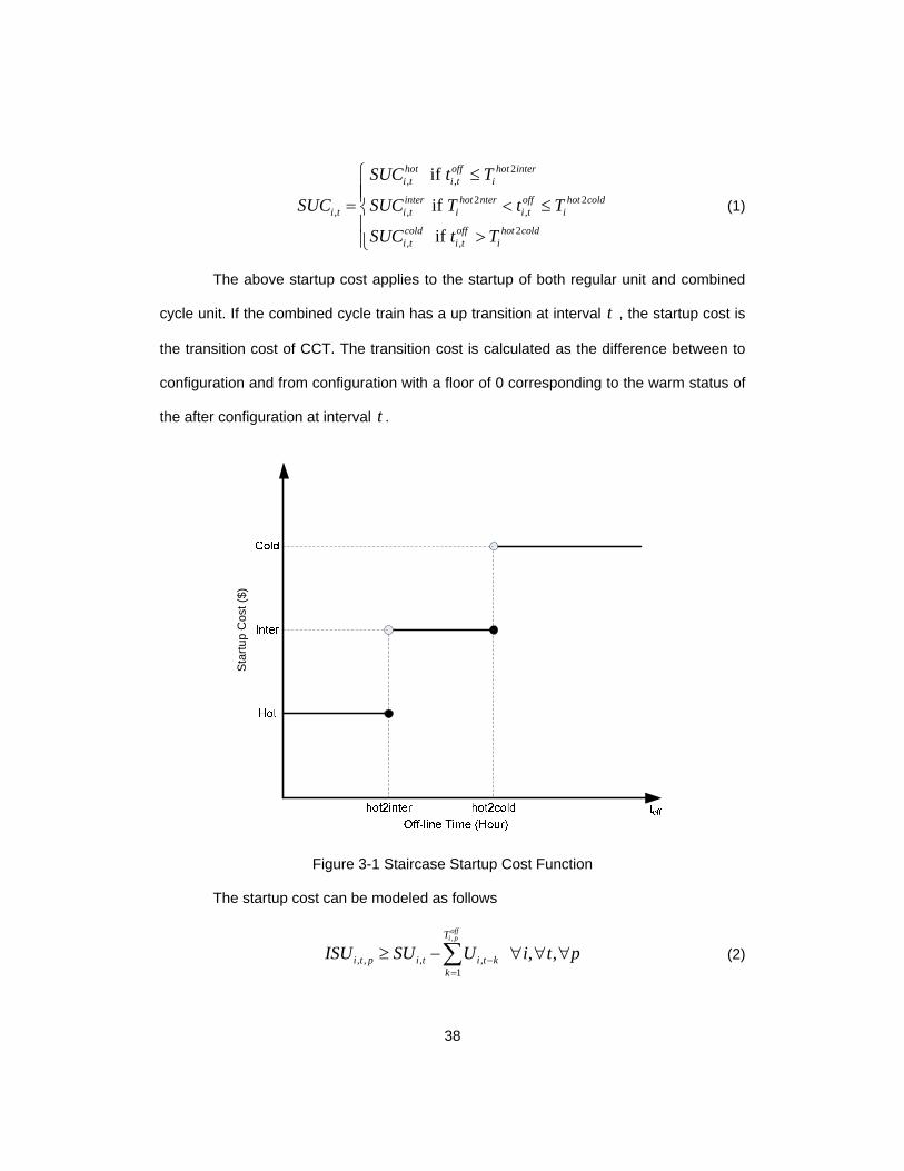
38
2, ,
2 2, , ,
2, ,
if
if
if
hot off hot interi t i t i
inter hot nter off hot coldi t i t i i t i
cold off hot coldi t i t i
SUC t T
SUC SUC T t T
SUC t T
(1)
The above startup cost applies to the startup of both regular unit and combined
cycle unit. If the combined cycle train has a up transition at interval t , the startup cost is
the transition cost of CCT. The transition cost is calculated as the difference between to
configuration and from configuration with a floor of 0 corresponding to the warm status of
the after configuration at interval t .
Sta
rtup
Cos
t ($)
Figure 3-1 Staircase Startup Cost Function
The startup cost can be modeled as follows
,
, , , ,1
, ,
offi pT
i t p i t i t kk
ISU SU U i t p
(2)

39
,
, , , ,1
* ,i tNP
i t p i t i tp
ISU SU NP i t
(3)
, , , , 1 , , 1i t p i t pISU ISU i t p (4)
,
1 1, , ,1 , , , , ,
2
* *( )i tNP
p pi t i t i t i t p i t i t
p
SUC ISU SUC ISU SUC SUC
(5)
The above startup cost applies to the startup of both regular unit and combined
cycle unit. If the combined cycle train has a up transition at interval t , the startup cost is
the transition cost of CCT. The transition cost is calculated as the difference between to
configuration and from configuration with a floor of 0 corresponding to the warm status of
the after configuration at interval t .
3.1.3 NCUC Solution Algorithm
As discussed in Chapter 2, the incremental energy offer curves in RUC are
piece-wise linear. Hence the RUC optimization cost functions calculated from the
integration of the incremental energy offer curves becomes quadratic. This makes the
RUC optimization problem as a mixed integer quadratic programming (MIQP) problem.
Compared to the linear MIP model, the MIQP model usually takes longer time to solve
and the performance is not desirable for the large RUC problem. To solve this issue, the
following two-step solution algorithm has been proposed for the NCUC:
Unit commitment (UC) step.
Economic dispatch (ED) step.
First, the UC step uses mixed integer programming (MIP) to solve the overall
problem by treating the piece-wise linear incremental cost curves as staircase constant.
Each segment of the incremental cost curve is modeled as a staircase curve as shown in
Figure 3-2. The number of horizontal segments used for the approximation is determined

40
in such a way that the areas between the original curve and the staircase segments
(shown as shadowed area in Figure 3-2) is less than a user defined constant. The UC
step determines the unit commitment schedules and binary variables including the unit
commitment decision variables and the ones used for the startup cost modeling. The
results of the binary variables from UC step are passed to ED step as fixed values.
Next, the ED step uses the quadratic programming (QP) to solve the same
problem again with the original cost curve but with all the binary variables fixed at the
solutions of the UC step. The ED step determines the unit dispatch schedules and market
clearing prices.
The mathematic programming language AMPL [12] is adopted to model the MIP
and QP problem and CPLEX [84] is utilized as the MIP and QP optimization solver.
Generation (MW) [LSL]
Q4
[HSL]Q3Q2
P1
P2
P3
P4
P5
Q1 Q5
MEO
Original Incremental Energy Cost Curve
Staircase approximation Curve
Min-Energy Cost=MEO*LSL
Figure 3-2 Incremental Cost Curve Approximation

41
3.1.4 NCUC Mathematic Formulation
The mathematic formulation of the NCUC is discussed as follows. The notation is
illustrated in Appendix A.
A. Objective Function
The NCUC optimization objective function is defined as the sum of startup cost,
minimum-energy cost and incremental energy cost.RUC also employs the penalty factors
on violation of security constraints (slack variables) in the objective function to ensure a
feasible solution.The NCUC objective function can be formulated as follows
, , , , ,1 1 1 1
, , ,1 1 1
Minimize
* *
NG T NPS T
i t i t i t i t s ti t s t
T NC T
pb el t es t lc lc tt c t
SUC MEC C P PSCOST
Penalty Slack Slack Penalty Slack
(6)
The offline time dependent startup cost is discussed in Section 3.1.2. The
resource minimum energy cost is formulated as below
min, , , ,* * ,i t i t i t i tMEC U MEO P i t (7)
The incremental energy cost is discussed in Section 3.1.3. The incremental
energy cost is linear term in UC step while it is quadratic term in ED step. The cost
function of the phase shifter tap position is discussed in Section 5.4. The penalty factors
are applied for the violation both the power balance constraint and transmission
constraints.
B. NCUC Constraints
The NCUC optimization problem is subject to various resource constraints and
security constraints shown as follows.
a) Power Balance Constraint
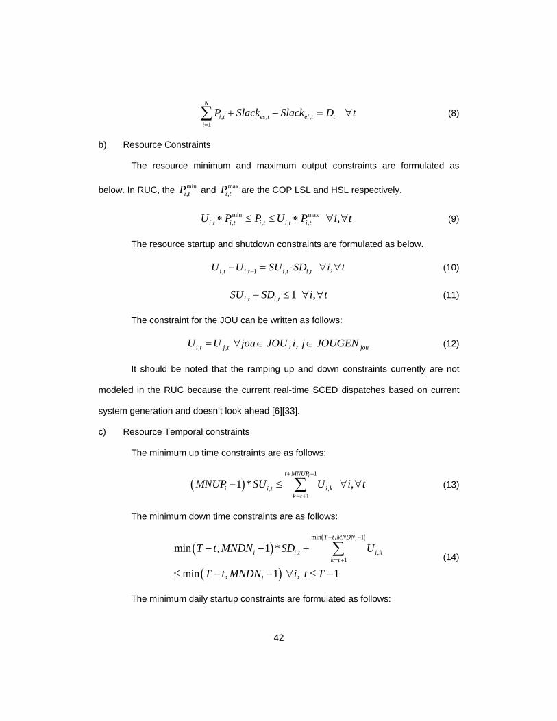
42
, , ,1
N
i t es t el t ti
P Slack Slack D t
(8)
b) Resource Constraints
The resource minimum and maximum output constraints are formulated as
below. In RUC, the min,i tP and max
,i tP are the COP LSL and HSL respectively.
min max, , , , , , i t i t i t i t i tU P P U P i t (9)
The resource startup and shutdown constraints are formulated as below.
, , 1 , ,- ,i t i t i t i tU U SU SD i t (10)
, , 1 ,i t i tSU SD i t (11)
The constraint for the JOU can be written as follows:
, , , ,i t j t jouU U jou JOU i j JOUGEN (12)
It should be noted that the ramping up and down constraints currently are not
modeled in the RUC because the current real-time SCED dispatches based on current
system generation and doesn’t look ahead [6][33].
c) Resource Temporal constraints
The minimum up time constraints are as follows:
1
, ,1
1 * ,it MNUP
i i t i kk t
MNUP SU U i t
(13)
The minimum down time constraints are as follows:
min , 1
, ,1
min , 1 *
min , 1 , 1
iT t MNDN
i i t i kk t
i
T t MNDN SD U
T t MNDN i t T
(14)
The minimum daily startup constraints are formulated as follows:

43
,1
T
i t it
SU MXSU i
(15)
d) Network Constraints
The transmission constraints considering the phase shifter impact is shown
below. The slack variables are applied here to model the transmission constraint
violation. The network constraint mathematic limit is discussed in detail in Section 3.2.
, , , , , ,1 1
* * NG NPS
MathLimitci t i t cs t s t lc t c t
i s
SF P SF PST Slack F c
(16)
C. Resource LMP
Once the NCUC optimization problem is solved, the resource LMP can be
calculated as below.
, , ,1
*NC
i t t ci t c tc
LMP SF SP
(17)
3.2 Network Security Monitor (NSM)
The function network security monitor (NSM), a.k.a. network security analysis
(NSA), evaluates the feasibility of the generation schedule for the intact (base case)
network as well as for the post-contingency network states. AC power flow results are
used to evaluate the feasibility of the base case. A linearized analysis is used to evaluate
the impact of the postulated contingencies. The NSM is performed for each interval of the
RUC study period to provide constraints for the NCUC function. For each violated
constraint, a set of shift factors is calculated with respect to generation resources. The
shift factors and the violated constraints are passed to the NCUC for enforcement.
The dynamic ratings for the transmission elements are used in the NSM. The
normal rating is used for base case power flow study and the emergency rating is used
for contingency analysis. In addition to the dynamic ratings, NSM also enforces a set of

44
generic constraints. The generic constraints are limitations on one or more transmission
elements which are used to protect the ERCOT transmission grid against transient
instability, dynamic instability or voltage collapse. The generic constraints are modeled by
NSM in both the base case and contingency analysis.
The NSM function supports load rollover schemes. A load rollover scheme
transfers a load at a node (source node) to one or more receiving nodes when a network
event causes the source node to be electrically de-energized. The receiving nodes may
be in the same station or in different stations. The network events that may cause a load
rollover include tripping of a breaker, outage of a transmission line or a transformer. If the
receiving nodes are also de-energized, NSM will drop the rollover load from the network.
NSM models all approved special protection systems (SPSs) and remedial action
plans (RAPs) while performing the contingency analysis. A SPS or RAP is a set of
automatic or pre-defined actions taken to relieve transmission security violations during
the post-contingency condition. These SPSs and RAPs are sufficiently dependable to
assume that they can be executed without loss of reliability to the ERCOT network. The
SPSs and RAPs will be used for contingency analysis before considering a resource
commitment and this logic will reduce the RUC over procurement.
As illustrated in Figure 3-3, the NSM consists of the following main components:
a) Network Data Update
Retrieves the network model prepared by the preprocessor and imposes on it the
latest NCUC generation schedule to establish the modified base case. The RUC Network
topology used by NSM is built based on the normal network and outage schedules. All
power flow computations uses a lossless model while satisfying the power flow
constraints. Transmission constraints are based on dynamic ratings.
b) Base Case Power Flow Solution

45
Performs non-linear AC power flow solution on the modified base case prepared
by network data update and computes the base case flows. A failure of the AC power
flow to converge automatically triggers the execution of the non-linear DC power flow.
c) Contingency Topology Processor
Prepares the final contingency list, violations check list and generator allocation
list for the DC contingency analysis.
d) Incremental Contingency Analysis
Performs Incremental (linear) contingency analysis by imposing contingencies
based on the lists prepared by the contingency topology processor and determines the
modified flows. If a SPS/RAP triggering condition is satisfied in a contingency, the
contingency shall be ignored, i.e., it is assumed that SPS/RAP clears all constraint
violations. NSM considers multilevel SPS/RAPS for breaker statuses, branch active
power flows and network bus voltages.
e) Constraint Data Processing
Selects the critical network violated constraints and computes the shift factors
(sensitivities) to be used by NCUC. The selection of critical network violated constraints is
based on the "constraint monitoring margin" parameter specified by the user. The base
case constraints and the worst contingency constraints with loading exceeding the
constraint-monitoring margin are automatically selected.
The NSM calculates the constraint mathematic limit and passes it to NCUC for
enforcement. The formulation of the network constraints mathematic limit can be
deduced as follows:

46
0
0
0
, , , ,
0 0, , , , , , , ,
, , , , , ,
0, , ,
* *
* *
* *
NCUC NSM NCUC PhysicalLimitc t c t c t c t
NSM PhysicalLimitc t ci t i t i t cs t s t s t c t
i s
PhysicalLimit NSMci t i t cs t s t c t c t
i s
ci t i t cs ti s
f f f F
f SF P P SF PST PST F
SF P SF PST F f
SF P SF PS
0
0,
, ,
, , , , ,
0 0, , , , , , ,
* *
* *
s t
NCUCMath MathLimitc t c t
NCUCMathc t ci t i t cs t s t
i s
MathLimit PhysicalLimit NSMc t c t c t ci t i t cs t s t
i s
T
f F
where f SF P SF PST
F F f SF P SF PST
(18)
The NSM Flow at previous iteration can be formulated as
0 0 0, , , , ,
0, , ,
* *
*
NSM neutralc t ci t i t cs t s t s
i s
offsetcn t n t c t
n
f SF P SF PST PST
SF NCV F
(19)
Substitute NSM Flow from above equation into NCUC Flow, the mathematic limit
is calculated as below.
0 0, , , , , ,
0 0 0, , , , , , ,
0, , , ,
* *
* * *
* *
MathLimit PhysicalLimitc t c t ci t i t cs t s t
i s
neutral offsetci t i t cs t s t s cn t n t c t
i s n
PhysicalLimit neutralc t cs t s cn t n t c
s n
F F SF P SF PST
SF P SF PST PST SF NCV F
F SF PST SF NCV F
,offsett
(20)
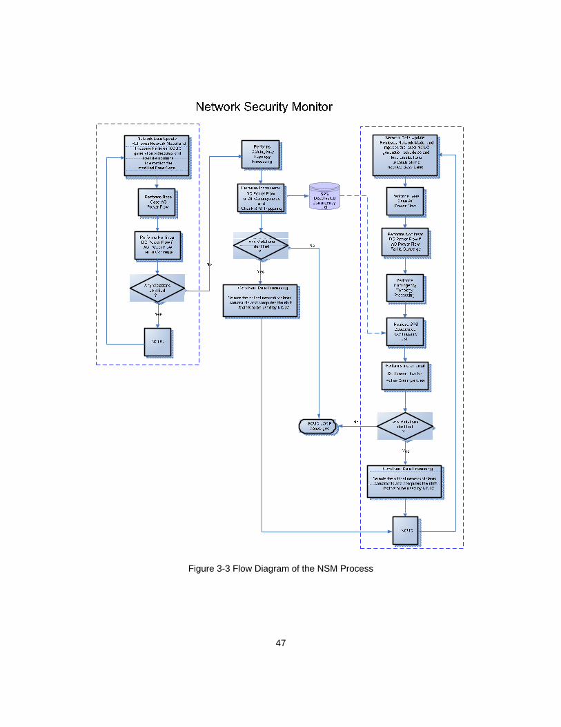
47
Figure 3-3 Flow Diagram of the NSM Process

48
3.3 RUC Clearing Process
The proposed RUC clearing process is shown in Figure 3-4. The NCUC and the
NSM iterates several times to determine the final solution. The steps in the proposed
solution process are as follows [6]:
1. Retrieve the initial base case data and superimpose on them the generation
schedule determined by the latest NCUC (or IUC) execution.
2. Invoke NSM for the base case at each time interval in the study period to identify
network constraints to be enforced in the NCUC solution.
3. Invoke NCUC to determine the revised generation schedule as impacted by enforcing
the additional network constraints.
4. Steps 2 and 3 iterate until convergence is reached.
5. SPS/RAP Triggering Test: using the solved NCUC generation at Step 4, invoke NSM
for all contingencies to test the SPS/RAP triggering conditions. Any contingencies
that trigger SPS/RAP are ignored in the subsequent NCUC-NSM iterations.
6. Invoke NSM for the base case and all contingencies without SPS/RAP triggering as
determined at Step 5 at each time interval in the study period to identify network
constraints to be enforced in the NCUC solution.
7. Invoke NCUC to determine the revised generation schedule as impacted by enforcing
the additional network constraints.
8. Step 6 and 7 iterate until convergence is reached.

49
Figure 3-4 NCUC-NSM Solution Process
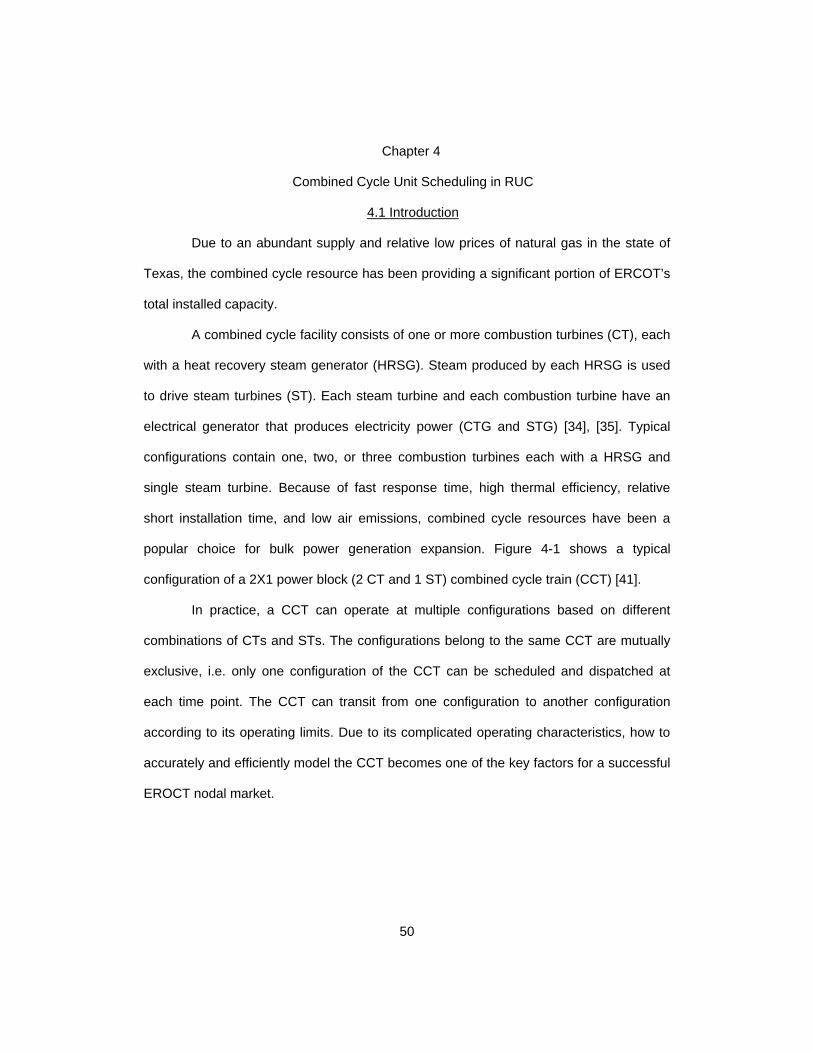
50
Chapter 4
Combined Cycle Unit Scheduling in RUC
4.1 Introduction
Due to an abundant supply and relative low prices of natural gas in the state of
Texas, the combined cycle resource has been providing a significant portion of ERCOT’s
total installed capacity.
A combined cycle facility consists of one or more combustion turbines (CT), each
with a heat recovery steam generator (HRSG). Steam produced by each HRSG is used
to drive steam turbines (ST). Each steam turbine and each combustion turbine have an
electrical generator that produces electricity power (CTG and STG) [34], [35]. Typical
configurations contain one, two, or three combustion turbines each with a HRSG and
single steam turbine. Because of fast response time, high thermal efficiency, relative
short installation time, and low air emissions, combined cycle resources have been a
popular choice for bulk power generation expansion. Figure 4-1 shows a typical
configuration of a 2X1 power block (2 CT and 1 ST) combined cycle train (CCT) [41].
In practice, a CCT can operate at multiple configurations based on different
combinations of CTs and STs. The configurations belong to the same CCT are mutually
exclusive, i.e. only one configuration of the CCT can be scheduled and dispatched at
each time point. The CCT can transit from one configuration to another configuration
according to its operating limits. Due to its complicated operating characteristics, how to
accurately and efficiently model the CCT becomes one of the key factors for a successful
EROCT nodal market.

51
Figure 4-1 A typical 2X1 combined cycle train configuration
Literatures provide various alternatives to model CCTs in electricity markets.
These alternatives try to balance the integrity of capturing the unique characteristics of
the CCTs and performance of conquering the complicated scheduling problem up to an
acceptable extent. This section reviews various ways of modeling of combined cycle
resources [34]-[40]:
Aggregate CCT modeling: This method simply represents a CCT by an aggregated
one that is treated as a regular thermal unit. The unit commitment and dispatch
decisions are made in each period with no regard to the state of each component.
However, this could be problematic since component unit technical constraints
cannot be correctly captured in this composite model.
Pseudo unit modeling (PSU): The model represents a CCT with one or more pseudo
units that comprise a single CT and its associated portion of the ST capacity. To
avoid inconsistent commitment, it is required that all PSUs have the same

52
characteristics (startup cost, minimum generation cost, minimum loading point,
incremental energy cost, minimum down time, and maximum capacity). As a
consequence, the PSU model has difficulties to precisely represent these
characteristics under different operating modes. The PSU approach has been
implemented successfully by ISO NE, NYISO, MISO, PJM, and IESO.
Configuration-based modeling: The approach models a combined cycle unit as
multiple mutually exclusive configurations or combinations of CT and ST. CCTs can
transition from one configuration to another one obeying predefined paths. The
approach allows each configuration to submit offer into a market independently.
Therefore, the flexibility would permit better representation of technical parameters
and bid data from each CCT. Currently, this approach has been implemented in the
CAISO MRTU market.
Physical unit modeling: This alternative is to model physical components of a CCT.
Each CT and ST is considered as an individual resource that may submit own startup
cost, minimum up/down time, incremental energy cost etc. From scheduling
perspective, this is not an ideal choice due to the complexity of handling dependency
among components. However, this model is naturally fit for the EMS, OTS, Outage
Scheduler, and other network security applications.
Generally speaking, the configuration-based model is more adequate for bid/offer
processing and dispatch scheduling, on the other hand, the physical unit modeling is
more adequate for the power flow and network security analysis.
4.2 Combined Cycle Unit Modeling in RUC
To satisfy both the network security requirements and the market optimization
needs associated with combined cycle trains, the new MMS for ERCOT nodal market is
required to support the modeling of CCT in two different ways:

53
Configuration-based modeling approach takes into account each operational
configuration of the combined-cycle train where each configuration is to be
considered as a separate resource in the optimization process. Each configuration
will be required to have its own distinct set of operating parameters, physical
constraints, energy, and AS offer curves.
Physical unit modeling is used in MMS while performing network security analysis.
Each combustion turbine (CT) and steam turbine (ST) associated with a combined
cycle facility is modeled as a separate unit. This approach is important to ensure an
accurate assessment of base case power flow, contingency analysis, and special
protection scheme (SPS) triggering conditions.
In 2007 the combined cycle resource conceptual design was accomplished to
allow CCT to offer each configuration as separate generation resources into the day-
ahead market. That allows a specified configuration of physical generation resources (CT
or ST) with a distinct set of operating parameters and physical constraints in CCT
registered with ERCOT. ERCOT’s resource registration system also has been expanded
to support for these additional parameters [41]. In April 2010, ERCOT submitted a nodal
protocol revision request (NPRR) to revise nodal protocol requirements to encompass
combined cycle resources. Two important definitions of combined cycle resources in the
NPRR are shown as follows:
Combined cycle train (CCT): The combinations of gas turbines and steam turbines in
an electric generation plant that employs more than one thermodynamic cycle. In
ERCOT Combined Cycle Trains are registered as a plant that can operate as a
generation resource in one or more combined cycle generation resource
configurations.

54
Combined cycle generation resource (CCGR): A specified configuration of physical
generation resources (gas and steam turbines), with a distinct set of operating
parameters and physical constraints, in a combined cycle train registered with
ERCOT.
As discussed in Chapter 3, the security constrained unit commitment (SCUC)
solution engine is used in the RUC clearing process to find the optimum commitment
schedules. The SCUC engine comprises two functional components: (a) network
constrained unit commitment (NCUC) and (b) network security monitor (NSM) [6][13][30].
The following sections describe the detailed CCU modeling approaches used in NCUC
and NSM.
4.2.1 CCU Modeling in NCUC
The NCUC function uses an advanced mixed integer programming (MIP)
technique to determine optimized commitment and dispatch schedules for RUC. In
NCUC, configuration-based CCT modeling is employed throughout. To reflect the
physical operating characteristics of CCT, the CCT in the nodal MMS is modeled by a set
of configurations (CCGR) along with the allowed transitions between the configurations
and transitions with the offline state. Each configuration is considered as a logical
resource. Similar to regular resources, each configuration has a distinct set of operating
parameters, physical constraints including:
Minimum online time.
Maximum online time.
Minimum offline time.
Hot, intermediate, cold startup times.
Maximum daily start up.
Maximum weekly start up (used only by WRUC).

55
Besides the data submitted for the regular units, the following additional data for
the CCT transition matrix is also needed:
CCT registration data including configuration name and associated physical
generators both primary and alternative to be used in case of primary generator is
disconnected or outaged.
Startup flag to indicate if the CCT can be startup to this configuration from offline.
Shutdown flag to indicate if the CCT can be shut down from this configuration to
offline.
List of allowed transitions specifying the
o From configuration
o To configuration
o Transition direction: up (additional generators are turned on) or down (some
generators are turned off)
Note that the startup transition can be considered as a special up transition from
the offline state. The shutdown transition can be considered as a special down transition
from online state. Table 4-1 lists the configuration registration data for a simple CCT with
2 CTs and 1 ST.
Table 4-1 CCT Configuration Registration
Configuration Name
ConfigurationType
Primary Unit
Alternative Unit
1 1CT+0ST CT1 CT2
2 2CT+0ST CT1,CT2
3 1CT+1ST CT1,ST CT2
4 2CT+1ST CT1,CT2,ST
Only CT units can be mutually alternate, and only ST units can be mutually
alternate, i.e. cannot replace CT with ST unit. If multiple alternative physical CCT
resources are specified for a CCT configuration then following rules are applied

56
sequentially in specified order to replace outaged or disconnected primary physical CCT
resources [30]:
Select alternative physical CCT resource with the highest voltage level of its
connectivity node.
Select alternative physical CCT resource with the highest capacity.
Select alternative physical CCT resource that is first in the database table, i.e.,
randomly.
Figure 4-2 shows the equivalent configurations with primary and alternative units.
Figure 4-2 Equivalent configurations with primary and alternative units
The state transition diagram for the above CCT can be shown in Figure 4-3.
Figure 4-3 CCT State Transition Diagram

57
A transition matrix can be derived from the state transition diagram between
configurations and offline (OFF) status. Table 4-2 lists the transition matrix derived from
the state transition diagram in Figure 4-3 where “” and “” denote the up and down
transitions respectively.
Table 4-2 CCT Transition Matrix
Transition Matrix To Configuration
OFF 1 2 3 4
Fro
m
Con
figur
atio
n
OFF
1
2
3
4
Above the main diagonal of the CCT transition matrix are upward transitions, i.e.
the transitions in which at least one physical CCT resource is started. Below the main
diagonal of CCT transition matrix are downward transitions, i.e. the transitions in which at
least one physical CCT resource is turned off.
Most costs and constraints affect CCT configurations in the same way as other
regular resources; however, the following additional logic applies to CCT:
Minimum online time only applies to up transitions. The online time of the after
transition is measured from the time when the configuration is started to the time
when it is shut down (i.e., the configuration is no longer on). Since the minimum
online time has already been satisfied in prior configuration, down transitions do not
need to be enforced.
The offline time is calculated using the following logic:
o For configurations that can startup: The number of hours offline is measured from
the time when the entire CCT is shut down to the CCT startup time.

58
o For configurations that transition in the up direction: The number of hours offline
is measured from the time when the configuration is shut down (i.e., the
configuration is no longer online) to the startup time.
o This calculated offline time is also used to determine the warmth state for startup
cost and startup time calculations.
The transition cost only applies to up transitions. It is calculated as the difference of
the startup cost between the after and before configurations.
Minimum offline time only applies to up transitions. The minimum offline time is not
applicable for down transitions because all the physical units in the after configuration
are online in the prior configuration.
The number of startups is calculated by measuring the number of up transitions
including startup for each configuration.
The energy constraint applies to each configuration separately.
The maximum on-line time applies to both the up and down transitions.
If the CCT is initially offline, then all configurations need to satisfy their respective
startup times.
Besides the constraints for the regular units in Section 3.1.4, the following extra
constraints are enforced for the combined cycle resources:
, , ,cc
i t cc ti CCGR
U U cc t
(21)
, 1 ,cc
i ti CCGR
U cc t
(22)
, , 1 , , 1( , )
(2 ) , ,cc
j t i t cc t cc t ccj i CCFT
U U U U cc i CCGR t
(23)
, 1 ,( , )
1 , ,cc
j t i t cci j CCIT
U U cc i CCGR t
(24)

59
, , 1 , ,cc
i t cc t cc ti CCGRSU
U U U cc t
(25)
, , , 1 ,cc
i t cc t cc ti CCGRSD
U U U cc t
(26)
4.2.2 CCU Modeling in NSM
The NSM function evaluates the feasibility of the generation schedule for the
intact (base case) network as well as for the post-contingency network states. NSM
function also models all approved special protection systems (SPSs) while performing the
contingency analysis. The NSM is performed for each interval of the RUC study to
provide constraints for the NCUC function. For each violated constraint, a set of shift
factors is calculated with respect to all controllable resources including CCTs. The shift
factors and the violated limits are passed to the NCUC for enforcement. The NCUC and
the NSM iterates several times to determine the final solution [6].
In NSM, physical modeling of the individual generators within a CCU facility is
important because the network models provided by network model management system
(NMMS) are specified at the physical generation unit level. In addition, all the contingency
definitions, outage schedules, and SPS triggering conditions are also defined at physical
unit level. While NCUC is using configuration-based modeling and NSM is using physical
unit-based modeling, a special interfacing mechanism needed to be established to allow
these two functions to exchange information.
A. Energy Schedule Disaggregation
The resulting optimal energy schedules determined by NCUC need to be
disaggregated to power outputs of physical CCT resources in order to be considered by
NSM function. This translation is performed using capacity weights (HRL) as distribution
factors. The optimal energy schedule for an online CC configuration ( CCGREnergySch ) is
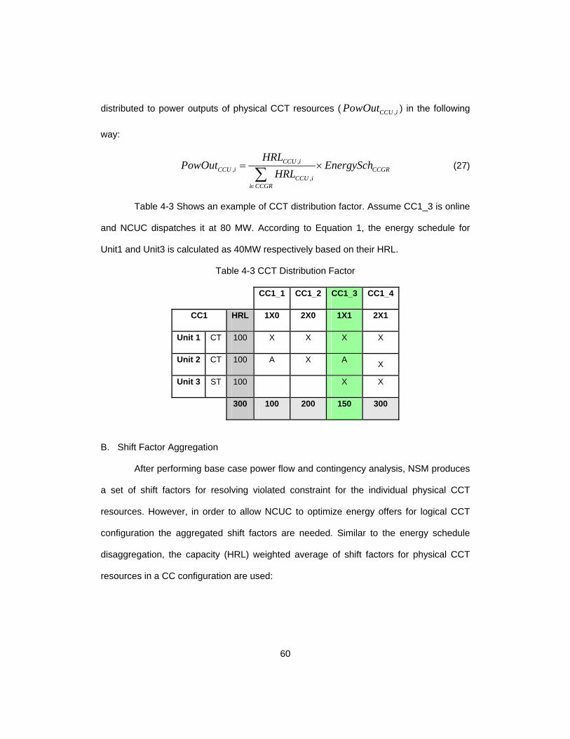
60
distributed to power outputs of physical CCT resources ( ,CCU iPowOut ) in the following
way:
,,
,
CCU iCCU i CCGR
CCU ii CCGR
HRLPowOut EnergySch
HRL
(27)
Table 4-3 Shows an example of CCT distribution factor. Assume CC1_3 is online
and NCUC dispatches it at 80 MW. According to Equation 1, the energy schedule for
Unit1 and Unit3 is calculated as 40MW respectively based on their HRL.
Table 4-3 CCT Distribution Factor
CC1_1 CC1_2 CC1_3 CC1_4
CC1 HRL 1X0 2X0 1X1 2X1
Unit 1 CT 100 X X X X
Unit 2 CT 100 A X A X
Unit 3 ST 100
X X
300 100 200 150 300
B. Shift Factor Aggregation
After performing base case power flow and contingency analysis, NSM produces
a set of shift factors for resolving violated constraint for the individual physical CCT
resources. However, in order to allow NCUC to optimize energy offers for logical CCT
configuration the aggregated shift factors are needed. Similar to the energy schedule
disaggregation, the capacity (HRL) weighted average of shift factors for physical CCT
resources in a CC configuration are used:

61
, ,
,
CCU i CCU ii CCGR
CCGRCCU i
i CCGR
HRL SFSF
HRL
(28)
Aggregated shift factors are calculated for all possible CCU configurations
(CCGR) and used accordingly within NCUC optimization process.
If there is a binding constraint and Unit1 has a shift factor 0.085 and Unit3 has a
shift factor 0.077 respectively w.r.t. the binding constraint. According to equation 28 NSM
calculates the aggregated shift factor for CC1_3 as
(0.085*100)+(0.077*100)/(100+100)=0.081.
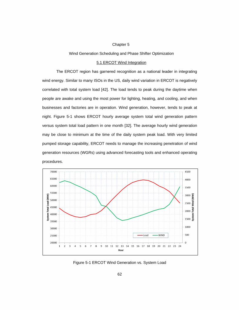
62
Chapter 5
Wind Generation Scheduling and Phase Shifter Optimization
5.1 ERCOT Wind Integration
The ERCOT region has garnered recognition as a national leader in integrating
wind energy. Similar to many ISOs in the US, daily wind variation in ERCOT is negatively
correlated with total system load [42]. The load tends to peak during the daytime when
people are awake and using the most power for lighting, heating, and cooling, and when
businesses and factories are in operation. Wind generation, however, tends to peak at
night. Figure 5-1 shows ERCOT hourly average system total wind generation pattern
versus system total load pattern in one month [32]. The average hourly wind generation
may be close to minimum at the time of the daily system peak load. With very limited
pumped storage capability, ERCOT needs to manage the increasing penetration of wind
generation resources (WGRs) using advanced forecasting tools and enhanced operating
procedures.
Figure 5-1 ERCOT Wind Generation vs. System Load

63
ERCOT has been experiencing several operational issues due to the growth of
WGRs. For instance, mismatch between the WGR forecast and actual output and the
high volatility of wind power generation create a challenge for maintaining system
frequency. ERCOT operators are forced to use more expensive ancillary reserves more
frequently in order to maintain frequency within the desired range. To address this issue,
ERCOT is improving wind generation forecast tool for real-time operation while making
changes to ancillary service requirement determination methodology to take into
consideration the effects of wind generation [42]-[45].
In addition, wind farms in ERCOT are concentrated in the West Texas area;
however, the major load centers are located in Dallas/Fort Worth and Houston areas.
The amount of power transferred from WGRs to the load centers is limited by the existing
transmission network capability. To fully utilize the available transfer capacity and take
advantage of the latest wind generation forecasting, ERCOT has implemented an hourly
limit calculation tool to monitor and enforce the latest transmission limits dynamically.
ERCOT also has implemented a set of special protection schemes (SPSs) and mitigation
plans to deal with local congestion issues that constrain the WGR generation [44]. In
addition, tap settings of certain phase shifting transformers, such as phase shifter at
Yellow Jacket, impact the maximum transmission capability from the ERCOT West
Incorrect phase shifter tap settings could result in inefficient market solutions and higher
market prices. To address this issue, a phase shifter optimization model has been
proposed and implemented in RUC to automatically determine the optimal phase shifter
tap settings.
As the installed generation capacity from WGRs grows rapidly, transmission
system of ERCOT also needs to be expanded quickly to provide necessary transmission
accesses for the new WGRs. How to allow customers to have access to the providers

64
whose energy is generated by WGRs became one of the major challenges for the
ERCOT system planning. In 2008, the Public Utility Commission of Texas (PUCT)
ordered ERCOT to conduct several competitive renewable energy zones (CREZs)
studies. Following the studies, the PUCT identified five CREZs in ERCOT based on the
concentration of WGR potentials and financial commitments demonstrated by the
developers. Later on, the PUCT further approved construction of 2,376 circuit miles of
new 345-kV transmission to be completed by the end of 2013 to support higher wind
penetration levels [46].
5.2 Short-Term Wind Generation Forecasting
Each hour ERCOT produces and updates a few types wind generation forecasts
for a rolling 48-hour in both system level and individual WGR level. The detail forecast
types are described as follows:
a) Total ERCOT wind power forecast (TEWPF): It represents a probability distribution of
the hourly production potential from all wind-power in ERCOT for each of the next 48
hours.
b) Short-Term wind power forecast (STWPF): it represents an hourly 50% probability of
exceedance forecast of the generation in MWh per hour from each WGR. ERCOT
uses the probabilistic TEWPF and select the forecast that the actual total ERCOT
WGR production is expected to exceed 50% of the time (50% probability of
exceedance forecast). To produce the STWPF, ERCOT allocates the TEWPF 50%
probability of exceedance forecast to each WGR such that the sum of the individual
STWPF forecasts equal the TEWPF forecast.
c) Wind-powered generation resource production potential (WGRPP): The generation in
MWh per hour from a WGR that could be generated from all available units of that
resource allocated from the 80% probability of exceedance of the TEWPF. WGRPP

65
is specific to each wind generator and is based on information provided by each
WGR, meteorological information, and data collected directly by ERCOT.
The WGRPP is lower than the STWPF for the same WGR since WGRPP is
produced as 80% probability of exceedance of the forecast while STWPF is produced as
50% probability of exceedance.
5.3 Wind Generation Scheduling in RUC
The WGRs are required to keep the COP up to date to reflect latest wind forecast
and changes in capacity or resource status. For the first 48 hours of the COP, a QSE
representing a WGR must enter an HSL value that is less than or equal to the most
recent STWPF provided by ERCOT for that WGR to show its production potential. The
balance of the 168 hours beyond 48-hours in the COP must also be provided by the QSE
for the WGR using its best estimate for the production potential. Originally Nodal
Protocols require WGR to enter HSL based on its WGRPP. Since WGRPP is more
conservative (i.e. lower) compared to STWPF, it may cause over commitment in RUC
and hence WGRPP was changed to STWPF as the basis for the HSLs in COP in a later
protocol revision.
Different from DAM, RUC is a reliability process and all the physical resources
including WGRs are required to participate in RUC by submitting a valid COP. Hence
both resource status and resource limits including HSL, LSL and ancillary service
schedules in the COP are used in RUC scheduling. The full capacity of HSL is
considered in RUC as maximum dispatch limit. Since WGRs are required to update their
COP HSL constantly based on the most current STWPF, RUC is able to take into
account the most recent WGR output potential in its scheduling from the WGR COP.
To verify the WGR COP HSL update accuracy, Figure 5-2 is drawn to show the
system total STWPF, WGRPP and WGR COP total HSL for operating day 12/06/2012 at

66
the snapshot of DRUC execution time (12/05/2012 14:30). The real-time wind generation
is also included in the figure for comparison. Figure 5-2 shows that the DRUC WGR COP
HSL is above WGRPP and close to STWPF as expected which indicates that QSE
followed the requirement to update the WGR COP according to the STWPF. All the 4
lines are following the same RT wind trend even they have differences due to forecasting
error in day ahead.
Figure 5-2 Wind Scheduling in DRUC
In RUC make-whole settlement, all QSEs that were capacity-short in each RUC
will be charged for that shortage as RUC capacity-short charge. To determine whether a
QSE is capacity-short, the WGRPP for the WGR used in the corresponding RUC is
considered the available capacity of the WGR when determining responsibility for the
corresponding RUC charges, regardless of the real-time output of the WGR. Even the
high value STWFP is used as HSL for RUC input to reduce RUC over commitment, the
low value WGRPP is used in RUC settlement to account for the WGR capacity.

67
5.4 Phase Shifter Optimization in RUC
5.4.1 Introduction
Currently, there are eight phase shifters installed and operated in the ERCOT
system. These phase shifters are primarily intended for relieving transmission overloads
caused by variations in wind generation. These phase shifters can be utilized to transfer
large amounts of power produced by WGRs from West Texas to ERCOT load centers
more effectively.
In real-time operation, ERCOT determines the transmission overloading
conditions and communicates the desired phase shifter tap settings to the phase shifter
Operators as required. The Phase Shifter Operators are responsible for adjusting the
Phase Shifters tap setting in real-time and telemeter the current tap setting to EMS
SCADA system. Based on the telemetered Phase Shifter tap settings, EMS state
estimator (SE) solves the base case power flow and the real-time contingency analysis
(RTCA) performs contingency analysis.
The detail phase shifter information is shown in Table 5-1. The step increment
indicates the phase angle change in degree per step change. All the eight phase shifters
have the same low, high and neutral step. The maximum degree change for each phase
shifter is ±1.875*16=±30 degree.
Table 5-1 Phase Shifter Parameters
No Phase Shifter Name Station Name
LowStep
HighStep
Neutral Step
Step Increment(degree)
1 BGLK_SOURCE_TAPS BGLK 1 33 17 1.875 2 FIREROCK_138_PS_H_4448 FIREROCK 1 33 17 1.875 3 HAMILTON_PS2_1335 HAMILTON 1 33 17 1.875 4 N_SHARPE_138_PS_1336 N_SHARPE 1 33 17 1.875 5 NLARSW_PST1_1337 NLARSW 1 33 17 1.875 6 PUTN_138_PS_1338 PUTN 1 33 17 1.875 7 THOMASTN_SR_THO1 THOMASTN 1 33 17 1.875 8 YELWJCKT_PS_1_H_4448 YELWJCKT 1 33 17 1.875

68
Figure 5-3 shows the ERCOT DAM LMP contour map for one operating hour.
The eight phase shifter locations are shown in the map as black dots with a number on
the side. It can be observed that the west zone has lower LMP compared to north zone
due to the binding constraint from west to north. It also shows that there are a small red
zone and a small blue zone in the west zone because there is binding local constraint
between them with the flow direction from the blue zone to the red zone.
Figure 5-3 ERCOT Phase Shifter Locations
In the beginning of nodal market, RUC did not have the capability to optimize the
phase shifter tap in their optimization engine. In order to model the impact of the phase

69
shifters, ERCOT system operations was requested to calculate an hourly tap position for
each phase shifter based on the WGR forecast and system load condition 2 days ahead
of operating day. Then the calculated tap positions were passed to RUC as fixed values
for network security analysis. This approach was better than the neutral settings for all
the hours but it also caused some market issues. This is because the calculation was
performed 2 days ahead with a lot of assumption and estimation and it could be much
different from real-time tap setting which can be freely adjusted according to real-time
operation condition. In some cases, the inaccurate calculated tap setting caused some
unrealistic congestion in RUC.
In order to solve the above issue and better model the phase shifters in RUC
scheduling, the enhancement of phase shifter tap optimization has been implemented in
RUC since July 2011. With this new enhancement, RUC Operator has the option to
enable or disable the optimization for each individual phase shifter in market operator
interface (MOI). When the phase shifter optimization is enabled, the hourly absolute
phase shifter tap positions are modeled as control variables in the optimization engine of
network security constrained unit commitment (NCUC). The shift factor of phase shifters
with respect to the transmission constraint is defined as MW/tap, i.e. the MW flow change
on the constraint with respect to each tap position change. In the NCUC, the cost function
for moving the tap is modeled as a positive V-shaped curve around the initial tap position
(not necessary the neutral tap position) with a very small slope ($/tap), e.g. 0.0001. One
example of the V-shaped cost curve is shown in Figure 5-4. In some cases, the initial tap
is set the same as neutral tap. The phase shifter tap positions are determined
automatically as part of RUC optimization solutions. If the phase shifter has impact to the
binding transmission constraint, it will be the most economic resource to be scheduled
away from its initial position to solve the congestion because the pre-defined cost for the

70
tap movement is set very small comparing with offer prices from regular resources.
Otherwise the phase shifter will be set at the initial tap position.
Figure 5-4 V-shaped Phase Shifter Movement Penalty Cost Function
5.4.2 Phase Shift Modeling in RUC
A. Power Injection Model of Phase Shifter
The one-line diagram of a transmission line with phase shifter is shown in Figure
5-5.
je
i j
i j
ijx
i
Figure 5-5 Transmission Line with Phase Shifter
Where i and j is the from bus and to bus respectively

71
i and j is phase angle at bus i and j respectively.
is the phase angle shift from the phase shifter.
ijx is the reactance of the transmission line in per unit.
The linear DC power flow on phase shifter from bus i to j bus is
i j i j
ijij ij ij
fx x x
(29)
According to the Equation above, the transmission line with phase shifter can be
equivalently treated as a normal line with reactance ijx and an withdrawn ijx
at bus i
and an injection ijx
at bus j .This equivalent treatment is referred as power injection
model (PIM) [89][90]. The equivalent power injection model of phase shifter can be
shown in Figure 5-6.
i j
ijx
ijx
ji
ijx
ijx
Figure 5-6 Phase Shifter Power Injection Model
B. Shift Factor of Phase Shifter
The shift factor of this phase shifter to a branch mn is defined as the change in
flow in branch mnmn f due to a change in unit angle ( ) (1 radian) of the phase
shifter angle. There is a fundamental difference in the manner by which phase shifter
sensitivities to a constraint is determined from the conventional shift factor determination
from a bus to a constraint.

72
Conceptually, when determining the shift factor from a bus to a constraint, one
can inject 1 MW at a bus and withdraw the same 1 MW at the slack (reference) bus and
determine how much of that 1 MW injection flows though the constraint (e.g. branch
mnmn f ). This approach directly gives the shift factor of this bus to the constraint.
For the shift factor from a phase shifter to a constraint, one need to change the
angle by 1 radian and observe how much the flow changes through the constraint (e.g.
branch mnmn f ). This approach directly gives the shift factor of the phase shifter to
this constraint. This is achieved by injecting 1 psx at bus i and 1 psx at bus j and
then determining the change in flow on the constraint (e.g. branch mnmn f ). The
equation below describes this.
Phase Shifter Shift factor PS radSF (MW/radian) to constraint on branch mn is:
1'
1
11 1
1
ps
ps radmn
ps
x
SF Bx
x
(30)
Where mnx is the per unit reactance of branch mn and
1 1 is the row vector with 0 in all locations except index m
(value=1) and n (value=-1) and

73
1 1T
ps psx x
is the column vector with 0 in all locations except
index i (value=1
psx
) and j (value=
1
psx
).
In the NCUC optimization the control variable is the phase shifter tap position,
therefore the shift factor derived above in terms of MW/radian needs to be transformed to
MW/tap.
ps tap ps radSF SF TapStepInRadians (31)
Where ps tapSF is the shift factor of phase shifter in MW/tap.
C. Cost Function of Phase Shifter
As illustrated in Figure 5-4, the cost function for moving the phase shifter tap in
the NCUC optimization is modeled as a positive V-shaped curve around the initial tap
position. The formulation is shown as follows:
, , 0 ,* ,ps t ps s t s tPSCOST C PST PST s t (32)

74
Chapter 6
RUC Study and Results Analysis
During the design phase of the nodal RUC project, a prototype RUC program
was developed with the proposed combined cycle unit (CCU) modeling to verify the
effectiveness of the CCU modeling. The prototype RUC program utilizes AMPL [12] as
modeling language and CPLEX [84] as optimization solver. The prototype RUC program
has been tested on a revised PJM 5-bus system [88] and the results are very promising.
Some of the test results are shown in Section 6.1 to illustrate the effectiveness of the
proposed algorithm. Because of the positive testing results, the proposed CCU modeling
has been adopted for the RUC project and eventually implemented for the production
RUC by the vendor and used in ERCOT.
For clarity and simplicity, first numerical cases running from the prototype RUC
program on the revised PJM 5-bus system are used to illustrate the primary features of
the RUC. Next the simulation results running from the production RUC software delivered
by the vendor on the real ERCOT system are presented to demonstrate the robustness
and effectiveness of the RUC clearing process.
6.1 RUC Study on PJM 5-bus Test System
The one-line diagram of the revised PJM 5-bus system [88] is shown in Figure
6-1. The revised PJM 5-bus system has 5 generation resources and 3 loads. To illustrate
the proposed combined cycle resource scheduling logic, the BRIGHTON resource is set
up as a combined cycle train (CCT) with 2 mutually exclusive configurations:
BRIGHTON_CC1_1 and BRIGHTON_CC1_2. The detail parameters of CCT
BRIGHTON_CC1 are listed in Table 6-1-Table 6-3.

75
Figure 6-1 Revised PJM 5-bus Test System
Table 6-1 BRIGHTON_CC1 Configuration Registration
Configuration Name Configuration Type Primary Unit Alternative Unit
BRIGHTON_CC1_1 1CT+1ST CT1,ST1 CT2
BRIGHTON_CC1_2 2CT+1ST CT1,CT2,ST1
Table 6-2 BRIGHTON_CC1 Transition Data
CCT Name From Configuration To Configuration Transition Direction
BRIGHTON_CC1 BRIGHTON_CC1_1 BRIGHTON_CC1_2 Upward
BRIGHTON_CC1 BRIGHTON_CC1_2 BRIGHTON_CC1_1 Downward
Table 6-3 BRIGHTON_CC1 Startup and Shutdown Flag
CCT Name Configuration Name Startup Flag Shutdown Flag
BRIGHTON_CC1 BRIGHTON_CC1_1 Y Y
BRIGHTON_CC1 BRIGHTON_CC1_2 N N
Table 6-4 Bus Load Distribution Factor of the 5-bus System
Bus A B C D EBus LDF 0 1/3 1/3 1/3 0

76
Table 6-5 Line Data of the 5-bus System
Line No From Bus To Bus R (%) X (%) Limit (MW)
1 A B 0 2.81 500
2 A D 0 3.04 500
3 A E 0 0.64 500
4 B C 0 1.08 500
5 C D 0 2.97 500
6 D E 0 2.97 240
The bus load distribution factor and line data of the 5-bus system are presented
in Table 6-4 and Table 6-5 respectively.
For simplicity, the DRUC scheduling logic is used for all the cases. The study
period is 24 hours of the next operating day and the study interval is 1 hour. The hour
ending (HE) convention is used in the study. To clearly illustrate the UC results, the
transmission constraint is only enforced in case 3 and all the other cases are tested in
unconstrained mode.
The resource parameters and resource three-part supply offers are listed in
Table 6-6 and Table 6-7 respectively. The three-part offer submitted by QSE is hourly
specific and can be different from hour to hour. Also the energy offer curve from the
three-part offer can be piece-wise linear and up to 10 break points. For clarity and
simplicity, each resource only has a constant three-part supply offer with only one
staircase segment energy offer curve
Table 6-6 Resource Parameters
Resource ID
Resource Name
Bus Pmin(MW)
Pmax(MW)
MNUP(Hour)
MNDN(Hour)
Hot2int(Hour)
Hot2cold (Hour)
MXUP
G1 ALTA A 11 110 4 5 3 5 3
G2 PARK CITY A 10 100 4 5 3 5 3
G3 SOLITUDE C 52 520 4 5 3 5 3
G4 SUNDANCE D 20 200 4 5 3 5 3
G5 BRIGHTON_CC1_1 E 100 300 4 5 8 20 3
G6 BRIGHTON_CC1_2 E 300 600 6 7 8 20 3
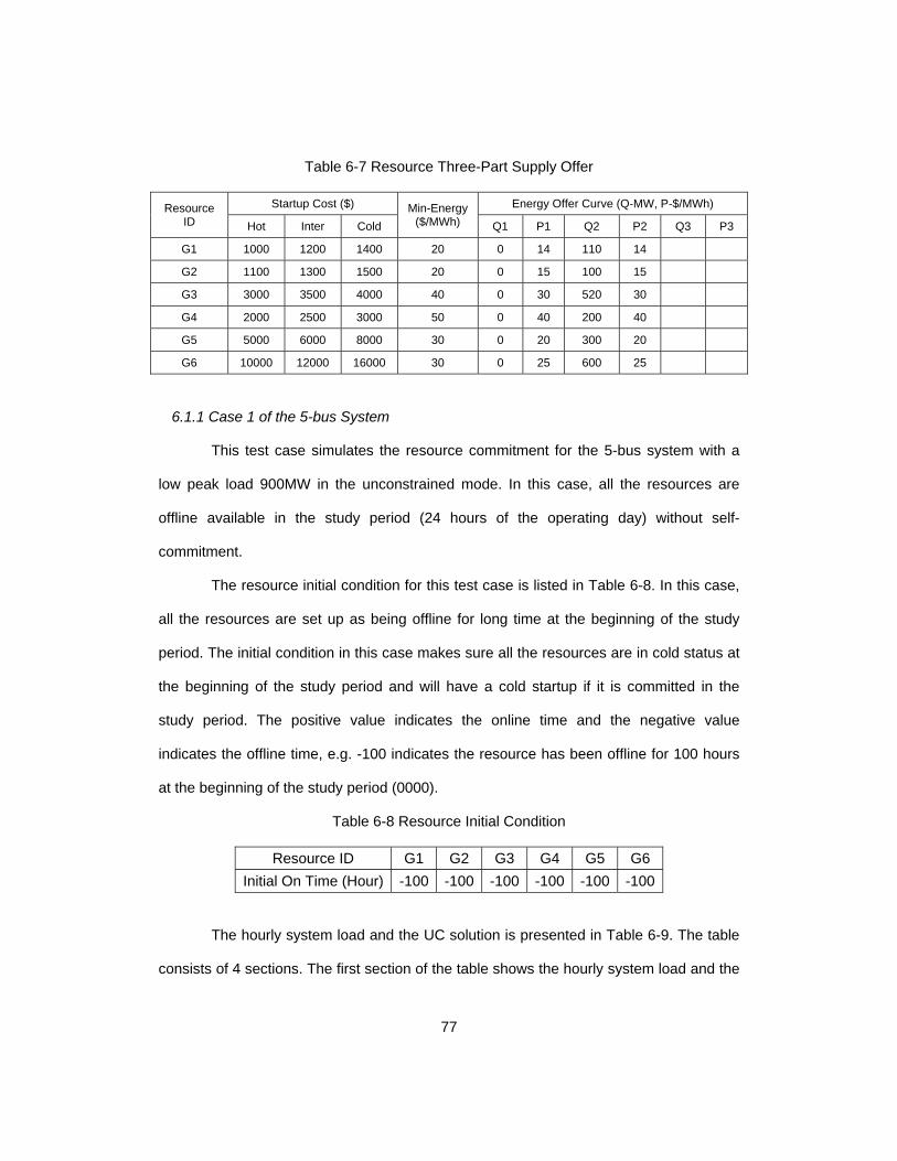
77
Table 6-7 Resource Three-Part Supply Offer
Resource ID
Startup Cost ($) Min-Energy($/MWh)
Energy Offer Curve (Q-MW, P-$/MWh)
Hot Inter Cold Q1 P1 Q2 P2 Q3 P3
G1 1000 1200 1400 20 0 14 110 14
G2 1100 1300 1500 20 0 15 100 15
G3 3000 3500 4000 40 0 30 520 30
G4 2000 2500 3000 50 0 40 200 40
G5 5000 6000 8000 30 0 20 300 20
G6 10000 12000 16000 30 0 25 600 25
6.1.1 Case 1 of the 5-bus System
This test case simulates the resource commitment for the 5-bus system with a
low peak load 900MW in the unconstrained mode. In this case, all the resources are
offline available in the study period (24 hours of the operating day) without self-
commitment.
The resource initial condition for this test case is listed in Table 6-8. In this case,
all the resources are set up as being offline for long time at the beginning of the study
period. The initial condition in this case makes sure all the resources are in cold status at
the beginning of the study period and will have a cold startup if it is committed in the
study period. The positive value indicates the online time and the negative value
indicates the offline time, e.g. -100 indicates the resource has been offline for 100 hours
at the beginning of the study period (0000).
Table 6-8 Resource Initial Condition
Resource ID G1 G2 G3 G4 G5 G6
Initial On Time (Hour) -100 -100 -100 -100 -100 -100
The hourly system load and the UC solution is presented in Table 6-9. The table
consists of 4 sections. The first section of the table shows the hourly system load and the

78
system lambda. The second section shows the resource commitment status for each
resource each hour: the value 0 with red color indicates that the resource is offline in this
hour and not committed, the value 1 with green color indicates that the resource is
committed online by UC and the value 1 with yellow color indicates that the resource is
self-committed online in COP by QSE. The third section shows resource hourly dispatch
and the fourth section shows resource hourly production cost which equals to the sum of
resource startup cost, min-gen cost and incremental energy cost. The total row under
section 2-4 is the sum for values of all the units for the specified hour, i.e. total number of
online resources, total dispatch MW and total production cost for the specified hour
respectively.
It shows that the system load is met by the generation for all the hours. Figure
6-2 shows the hourly system load and system lambda for the 24 hour study period. It can
be observed that the system lambda is high during peak hours and is low at off-peak.
Figure 6-2 Case 1 System Load and System Lambda

79
Table 6-9 Case 1 Hourly System Load and UC Solution
HE 1 2 3 4 5 6 7 8 9 10 11 12 13 14 15 16 17 18 19 20 21 22 23 24
Load 350 300 250 200 250 300 400 500 550 600 650 700 750 800 850 875 900 800 700 600 550 500 450 400
SL 20 15 15 14 15 15 20 20 20 30 30 30 30 30 30 30 30 30 30 30 20 20 20 20
Unit 1 2 3 4 5 6 7 8 9 10 11 12 13 14 15 16 17 18 19 20 21 22 23 24
G1 1 1 1 1 1 1 1 1 1 1 1 1 1 1 1 1 1 1 1 1 1 1 1 1
G2 1 1 1 1 1 1 1 1 1 1 1 1 1 1 1 1 1 1 1 1 1 1 1 1
G3 0 0 0 0 0 0 0 0 1 1 1 1 1 1 1 1 1 1 1 1 1 0 0 0
G4 0 0 0 0 0 0 0 0 0 0 0 0 0 0 0 0 0 0 0 0 0 0 0 0
G5 1 1 1 1 1 1 1 1 1 1 1 1 1 1 1 1 1 1 1 1 1 1 1 1
G6 0 0 0 0 0 0 0 0 0 0 0 0 0 0 0 0 0 0 0 0 0 0 0 0
Total 3 3 3 3 3 3 3 3 4 4 4 4 4 4 4 4 4 4 4 4 4 3 3 3
Unit 1 2 3 4 5 6 7 8 9 10 11 12 13 14 15 16 17 18 19 20 21 22 23 24
G1 110 110 110 90 110 110 110 110 110 110 110 110 110 110 110 110 110 110 110 110 110 110 110 110
G2 100 90 40 10 40 90 100 100 100 100 100 100 100 100 100 100 100 100 100 100 100 100 100 100
G3 0 0 0 0 0 0 0 0 52 90 140 190 240 290 340 365 390 290 190 90 52 0 0 0
G4 0 0 0 0 0 0 0 0 0 0 0 0 0 0 0 0 0 0 0 0 0 0 0 0
G5 140 100 100 100 100 100 190 290 288 300 300 300 300 300 300 300 300 300 300 300 288 290 240 190
G6 0 0 0 0 0 0 0 0 0 0 0 0 0 0 0 0 0 0 0 0 0 0 0 0
Total 350 300 250 200 250 300 400 500 550 600 650 700 750 800 850 875 900 800 700 600 550 500 450 400
Unit 1 2 3 4 5 6 7 8 9 10 11 12 13 14 15 16 17 18 19 20 21 22 23 24
G1 3006 1606 1606 1326 1606 1606 1606 1606 1606 1606 1606 1606 1606 1606 1606 1606 1606 1606 1606 1606 1606 1606 1606 1606
G2 3050 1400 650 200 650 1400 1550 1550 1550 1550 1550 1550 1550 1550 1550 1550 1550 1550 1550 1550 1550 1550 1550 1550
G3 0 0 0 0 0 0 0 0 6080 3220 4720 6220 7720 9220 10720 11470 12220 9220 6220 3220 2080 0 0 0
G4 0 0 0 0 0 0 0 0 0 0 0 0 0 0 0 0 0 0 0 0 0 0 0 0
G5 11800 3000 3000 3000 3000 3000 4800 6800 6760 7000 7000 7000 7000 7000 7000 7000 7000 7000 7000 7000 6760 6800 5800 4800
G6 0 0 0 0 0 0 0 0 0 0 0 0 0 0 0 0 0 0 0 0 0 0 0 0
Total 17856 6006 5256 4526 5256 6006 7956 9956 15996 13376 14876 16376 17876 19376 20876 21626 22376 19376 16376 13376 11996 9956 8956 7956
System Load (MW) and System Lambda ($/MWh) for Each Hour
Resource Commitment Status for Each Hour
Resource Dispatch (MW) for Each Hour
Resource Production Cost ($) for Each Hour
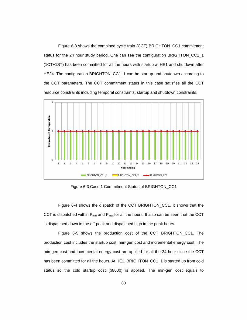
80
Figure 6-3 shows the combined cycle train (CCT) BRIGHTON_CC1 commitment
status for the 24 hour study period. One can see the configuration BRIGHTON_CC1_1
(1CT+1ST) has been committed for all the hours with startup at HE1 and shutdown after
HE24. The configuration BRIGHTON_CC1_1 can be startup and shutdown according to
the CCT parameters. The CCT commitment status in this case satisfies all the CCT
resource constraints including temporal constraints, startup and shutdown constraints.
Figure 6-3 Case 1 Commitment Status of BRIGHTON_CC1
Figure 6-4 shows the dispatch of the CCT BRIGHTON_CC1. It shows that the
CCT is dispatched within Pmin and Pmax for all the hours. It also can be seen that the CCT
is dispatched down in the off-peak and dispatched high in the peak hours.
Figure 6-5 shows the production cost of the CCT BRIGHTON_CC1. The
production cost includes the startup cost, min-gen cost and incremental energy cost. The
min-gen cost and incremental energy cost are applied for all the 24 hour since the CCT
has been committed for all the hours. At HE1, BRIGHTON_CC1_1 is started up from cold
status so the cold startup cost ($8000) is applied. The min-gen cost equals to

81
MEO*Pmin=30*100=$3000. The incremental cost is 20*(140MW-100MW)=$800. So the
production cost=startup cost ($8000)+min-gen cost ($3000)+incremental energy cost
($800)=$11800. This is consistent with the production cost at HE1 for the CCT.
Figure 6-4 Case 1 Dispatch of BRIGHTON_CC1
Figure 6-5 Case 1 Production Cost of BRIGHTON_CC1

82
6.1.2 Case 2 of the 5-bus System
Case 2 has the same input as case 1 except the system load has been increased
with peak load as 1400MW. The hourly system load and the UC solution is presented in
Table 6-10.
Figure 6-6 shows the hourly system load and system lambda for the 24 hour
study period. It can be observed that the system lambda is $30/MWh for all the hours
except at HE17 and HE4. HE4 has the lowest load in the study period and the system
lambda is 20$/MWh. HE17 has the peak load 1400MW and the system lambda is
$40/MWh.
Figure 6-6 Case 2 System Load and System Lambda

83
Table 6-10 Case 2 Hourly System Load and UC Solution
HE 1 2 3 4 5 6 7 8 9 10 11 12 13 14 15 16 17 18 19 20 21 22 23 24
Load 700 650 600 550 600 700 800 850 900 950 1000 1050 1100 1150 1200 1300 1400 1320 1250 1120 1080 920 820 760
SL 30 30 30 20 30 30 30 30 30 30 30 30 30 30 30 30 40 30 30 30 30 30 30 30
Unit 1 2 3 4 5 6 7 8 9 10 11 12 13 14 15 16 17 18 19 20 21 22 23 24
G1 1 1 1 1 1 1 1 1 1 1 1 1 1 1 1 1 1 1 1 1 1 1 1 1
G2 1 1 1 1 1 1 1 1 1 1 1 1 1 1 1 1 1 1 1 1 1 1 1 1
G3 1 1 1 1 1 1 1 1 1 1 1 1 1 1 1 1 1 1 1 1 1 1 1 1
G4 0 0 0 0 0 0 0 0 0 0 0 0 0 0 0 0 1 0 0 0 0 0 0 0
G5 1 1 1 1 1 1 1 1 1 1 1 0 0 0 0 0 0 0 0 0 0 1 1 1
G6 0 0 0 0 0 0 0 0 0 0 0 1 1 1 1 1 1 1 1 1 1 0 0 0
Total 4 4 4 4 4 4 4 4 4 4 4 4 4 4 4 4 5 4 4 4 4 4 4 4
Unit 1 2 3 4 5 6 7 8 9 10 11 12 13 14 15 16 17 18 19 20 21 22 23 24
G1 110 110 110 110 110 110 110 110 110 110 110 110 110 110 110 110 110 110 110 110 110 110 110 110
G2 100 100 100 100 100 100 100 100 100 100 100 100 100 100 100 100 100 100 100 100 100 100 100 100
G3 190 140 90 52 90 190 290 340 390 440 490 240 290 340 390 490 520 510 440 310 270 410 310 250
G4 0 0 0 0 0 0 0 0 0 0 0 0 0 0 0 0 70 0 0 0 0 0 0 0
G5 300 300 300 288 300 300 300 300 300 300 300 0 0 0 0 0 0 0 0 0 0 300 300 300
G6 0 0 0 0 0 0 0 0 0 0 0 600 600 600 600 600 600 600 600 600 600 0 0 0
Total 700 650 600 550 600 700 800 850 900 950 1000 1050 1100 1150 1200 1300 1400 1320 1250 1120 1080 920 820 760
Unit 1 2 3 4 5 6 7 8 9 10 11 12 13 14 15 16 17 18 19 20 21 22 23 24
G1 3006 1606 1606 1606 1606 1606 1606 1606 1606 1606 1606 1606 1606 1606 1606 1606 1606 1606 1606 1606 1606 1606 1606 1606
G2 3050 1550 1550 1550 1550 1550 1550 1550 1550 1550 1550 1550 1550 1550 1550 1550 1550 1550 1550 1550 1550 1550 1550 1550
G3 10220 4720 3220 2080 3220 6220 9220 10720 12220 13720 15220 7720 9220 10720 12220 15220 16120 15820 13720 9820 8620 12820 9820 8020
G4 0 0 0 0 0 0 0 0 0 0 0 0 0 0 0 0 6000 0 0 0 0 0 0 0
G5 15000 7000 7000 6760 7000 7000 7000 7000 7000 7000 7000 0 0 0 0 0 0 0 0 0 0 7000 7000 7000
G6 0 0 0 0 0 0 0 0 0 0 0 24500 16500 16500 16500 16500 16500 16500 16500 16500 16500 0 0 0
Total 31276 14876 13376 11996 13376 16376 19376 20876 22376 23876 25376 35376 28876 30376 31876 34876 41776 35476 33376 29476 28276 22976 19976 18176
System Load (MW) and System Lambda ($/MWh) for Each Hour
Resource Commitment Status for Each Hour
Resource Dispatch (MW) for Each Hour
Resource Production Cost ($) for Each Hour

84
Figure 6-7 shows the combined cycle train (CCT) BRIGHTON_CC1 commitment
status for the 24 hour study period. One can see the configuration BRIGHTON_CC1_1
(1CT+1ST) has been committed for HE1-HE11. BRIGHTON_CC1_1 has been online for
11 hours that satisfies its minimum online time (6 hours). At HE12 the configuration
BRIGHTON_CC1_1 is transited up to configuration BRIGHTON_CC1_2. Configuration
BRIGHTON_CC1_2 stays online until HE21 and it transits down to configuration
BRIGHTON_CC1_1 at HE22. Then BRIGHTON_CC1_1 stays online until HE24.
Configuration BRIGHTON_CC1_2 has met both the minimum online time (6 hours) and
minimum offline time (6 hours) during the online period. Because DRUC only covers one
operating day, DRUC assumes that all units including CCT are offline after the end of the
study period. Since BRIGHTON_CC1_2 can’t be shutdown according to the CCT
shutdown constraints in Table 6-3, BRIGHTON_CC1_2 is transited down to
BRIGHTON_CC1_1 at HE22 which can be shut down after HE24 to meet the shutdown
constraint. As described in the CCU modeling, the minimum online time is only enforced
for the up transition and is not enforced for the down transition. Because of this logic,
BRIGHTON_CC1_1 stays online for only 3 hours from HE22 to HE24 after the down
transition which is less than its 6 hour minimum online time. The CCT commitment status
in this case satisfies all the CCT resource constraints including temporal constraints,
startup and shutdown constraints.
Figure 6-8 shows the dispatch of the CCT BRIGHTON_CC1. It shows that the
CCT is dispatched within Pmin and Pmax for the corresponding configuration for all the
hours. During HE1-HE11 and HE22-HE24, BRIGHTON_CC1_1 is dispatched and the
dispatch MW is less or equal to its Pmax 300MW. During HE12-HE21, the CCT is in a
higher configuration BRIGHTON_CC1_2 and it is fully dispatched to its Pmax 600MW.

85
Figure 6-7 Case 2 Commitment Status of BRIGHTON_CC1
Figure 6-8 Case 2 Dispatch of BRIGHTON_CC1
Figure 6-9 shows the production cost of the CCT BRIGHTON_CC1. At HE1,
BRIGHTON_CC1_1 is started up from cold status so the cold startup cost ($8000) is
applied. The min-gen cost equals to MEO*Pmin=30*100=$3000. The incremental cost is
20*(300MW-100MW)=$4000. So the production cost=startup cost ($8000)+min-gen cost
($3000)+incremental energy cost ($4000)=$15000. This is consistent with the production

86
cost at HE1 for the CCT. At HE12, BRIGHTON_CC1_1 is transited up to
BRIGHTON_CC1_2 and the up transition cost is applied in this hour. Since
BRIGHTON_CC1_2 has been offline for long time and in cold status, the cold transition
cost is applied. As described in the CCU modeling, the transition cost is calculated as the
difference of the startup cost between the after and before configurations for the warm
status of the after configuration. In this case, the cold transition cost=
BRIGHTON_CC1_2 cold startup cost - BRIGHTON_CC1_1 cold startup cost=16000-
8000=$8000. The min-gen cost equals to MEO*Pmin=30*300=$9000. The incremental
cost is 25*(600MW-300MW)=$7500. So the production cost=transition cost ($8000)+min-
gen cost ($9000)+incremental energy cost ($7500)=$24500. This is consistent with the
production cost at HE12 for the CCT. At HE22, BRIGHTON_CC1_2 is transited down to
BRIGHTON_CC1_1 and the transition cost is not applied for the down transition in this
hour. So the production cost=transition cost ($0)+min-gen cost ($3000)+incremental
energy cost ($4000)=$7000. This is consistent with the production cost at HE22 for the
CCT.
Figure 6-9 Case 2 Production Cost of BRIGHTON_CC1

87
6.1.3 Case 3 of the 5-bus System
This case simulates resource commitment and scheduling with transmission
constraint enforced in the optimization. The same input data from case 2 is adopted for
this case. In addition, the base case flow on line ED is enforced in the UC for this case.
For simplicity, only the base case constraint is modeled in the study. The same logic
used for the base case constraint can be applied to the contingency constraint.
The base case bus shift factor w.r.t to line ED can be calculated based on the
line data listed in Table 6-5. Assume bus A is the slack bus, the bus shift factors w.r.t. line
ED is listed in Table 6-11.
Table 6-11 Bus Shift Factor w.r.t. Line ED of the 5-bus System
Bus A B C D E Shift Factor 0 -0.1509 -0.209 -0.3685 0.112
The hourly system load and the UC solution for this case is presented in Table
6-12. It can be observed that the committed pattern has changed for G4, G5 and G6. G4
has negative shift factor -0.3685 w.r.t. the line ED and G5 and G6 has positive shift factor
0.112 w.r.t. the line. G4 is more expensive than G5 and G6 and it is only committed for
HE17 in unconstrained case 2. In case 3 to solve the congestion, G4 is committed for
HE12-HE21 and G6 is only committed for HE14-HE19.
Figure 6-10 shows the hourly system load and system lambda for the 24 hour
study period. It can be observed that the system lambda is lower during the peak hours
HE14-HE19.

88
Figure 6-10 Case 3 System Load and System Lambda
Figure 6-11 shows the comparison of line ED flow between case 2 and case 3.
One can see that the line flow in case 2 exceeds the line limit 240MW during HE12-HE21
since the transmission constraint is not enforced in case 2. One also see that the line flow
in case 3 is less than or equal to the line limit 240MW during HE12-HE21 which illustrates
that the transmission constraint is enforced in case 3 as expected. Figure 6-12 shows the
hourly system production cost comparison between unconstrained case 2 and
constrained case 3. It can be observed in some hours the hourly production cost in
constrained case 3 is less than the production cost in unconstrained case 2. But the total
production cost across the 24 hours from constrained case 3 is greater than the one from
case 2 since the additional transmission constraint is introduced in case 3.
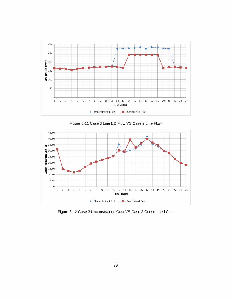
89
Figure 6-11 Case 3 Line ED Flow VS Case 2 Line Flow
Figure 6-12 Case 3 Unconstrained Cost VS Case 2 Constrained Cost

90
Table 6-12 Case 3 Hourly System Load and UC Solution
HE 1 2 3 4 5 6 7 8 9 10 11 12 13 14 15 16 17 18 19 20 21 22 23 24
Load 700 650 600 550 600 700 800 850 900 950 1000 1050 1100 1150 1200 1300 1400 1320 1250 1120 1080 920 820 760
SL 30 30 30 20 30 30 30 30 30 30 30 30 40 26.74 26.74 28.50 28.50 28.50 28.50 40 40 30 30 30
Unit 1 2 3 4 5 6 7 8 9 10 11 12 13 14 15 16 17 18 19 20 21 22 23 24
G1 1 1 1 1 1 1 1 1 1 1 1 1 1 1 1 1 1 1 1 1 1 1 1 1
G2 1 1 1 1 1 1 1 1 1 1 1 1 1 1 1 1 1 1 1 1 1 1 1 1
G3 1 1 1 1 1 1 1 1 1 1 1 1 1 1 1 1 1 1 1 1 1 1 1 1
G4 0 0 0 0 0 0 0 0 0 0 0 1 1 1 1 1 1 1 1 1 1 0 0 0
G5 1 1 1 1 1 1 1 1 1 1 1 1 1 0 0 0 0 0 0 1 1 1 1 1
G6 0 0 0 0 0 0 0 0 0 0 0 0 0 1 1 1 1 1 1 0 0 0 0 0
Total 4 4 4 4 4 4 4 4 4 4 4 5 5 5 5 5 5 5 5 5 5 4 4 4
Unit 1 2 3 4 5 6 7 8 9 10 11 12 13 14 15 16 17 18 19 20 21 22 23 24
G1 110 110 110 110 110 110 110 110 110 110 110 110 110 110 110 110 110 110 110 110 110 110 110 110
G2 100 100 100 100 100 100 100 100 100 100 100 100 100 100 100 100 100 100 100 100 100 100 100 100
G3 190 140 90 52 90 190 290 340 390 440 490 520 520 420.2 475.5 520 520 520 520 520 520 410 310 250
G4 0 0 0 0 0 0 0 0 0 0 0 20 70 20 20 64.1 137.9 78.87 27.18 90 50 0 0 0
G5 300 300 300 288 300 300 300 300 300 300 300 300 300 0 0 0 0 0 0 300 300 300 300 300
G6 0 0 0 0 0 0 0 0 0 0 0 0 0 499.8 494.5 505.9 532.1 511.1 492.8 0 0 0 0 0
Total 700 650 600 550 600 700 800 850 900 950 1000 1050 1100 1150 1200 1300 1400 1320 1250 1120 1080 920 820 760
Unit 1 2 3 4 5 6 7 8 9 10 11 12 13 14 15 16 17 18 19 20 21 22 23 24
G1 3006 1606 1606 1606 1606 1606 1606 1606 1606 1606 1606 1606 1606 1606 1606 1606 1606 1606 1606 1606 1606 1606 1606 1606
G2 3050 1550 1550 1550 1550 1550 1550 1550 1550 1550 1550 1550 1550 1550 1550 1550 1550 1550 1550 1550 1550 1550 1550 1550
G3 10220 4720 3220 2080 3220 6220 9220 10720 12220 13720 15220 16120 16120 13127 14784 16120 16120 16120 16120 16120 16120 12820 9820 8020
G4 0 0 0 0 0 0 0 0 0 0 0 4000 3000 1000 1000 2764 5718 3355 1287 3800 2200 0 0 0
G5 15000 7000 7000 6760 7000 7000 7000 7000 7000 7000 7000 7000 7000 0 0 0 0 0 0 7000 7000 7000 7000 7000
G6 0 0 0 0 0 0 0 0 0 0 0 0 0 21995 13863 14148 14802 14278 13820 0 0 0 0 0
Total 31276 14876 13376 11996 13376 16376 19376 20876 22376 23876 25376 30276 29276 39277 32803 36187 39795 36909 34384 30076 28476 22976 19976 18176
System Load (MW) and System Lambda ($/MWh) for Each Hour
Resource Commitment Status for Each Hour
Resource Dispatch (MW) for Each Hour
Resource Production Cost ($) for Each Hour
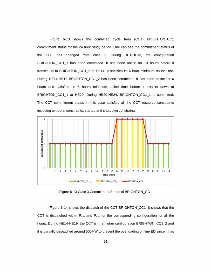
91
Figure 6-13 shows the combined cycle train (CCT) BRIGHTON_CC1
commitment status for the 24 hour study period. One can see the commitment status of
the CCT has changed from case 2. During HE1-HE13, the configuration
BRIGHTON_CC1_1 has been committed. It has been online for 13 hours before it
transits up to BRIGHTON_CC1_2 at HE14. It satisfies its 6 hour minimum online time.
During HE14-HE19 BRIGHTON_CC1_2 has been committed. It has been online for 6
hours and satisfies its 6 hours minimum online time before it transits down to
BRIGHTON_CC1_1 at HE20. During HE20-HE24, BRIGHTON_CC1_1 is committed.
The CCT commitment status in this case satisfies all the CCT resource constraints
including temporal constraints, startup and shutdown constraints.
Figure 6-13 Case 3 Commitment Status of BRIGHTON_CC1
Figure 6-14 shows the dispatch of the CCT BRIGHTON_CC1. It shows that the
CCT is dispatched within Pmin and Pmax for the corresponding configuration for all the
hours. During HE14-HE19, the CCT is in a higher configuration BRIGHTON_CC1_2 and
it is partially dispatched around 500MW to prevent the overloading on line ED since it has
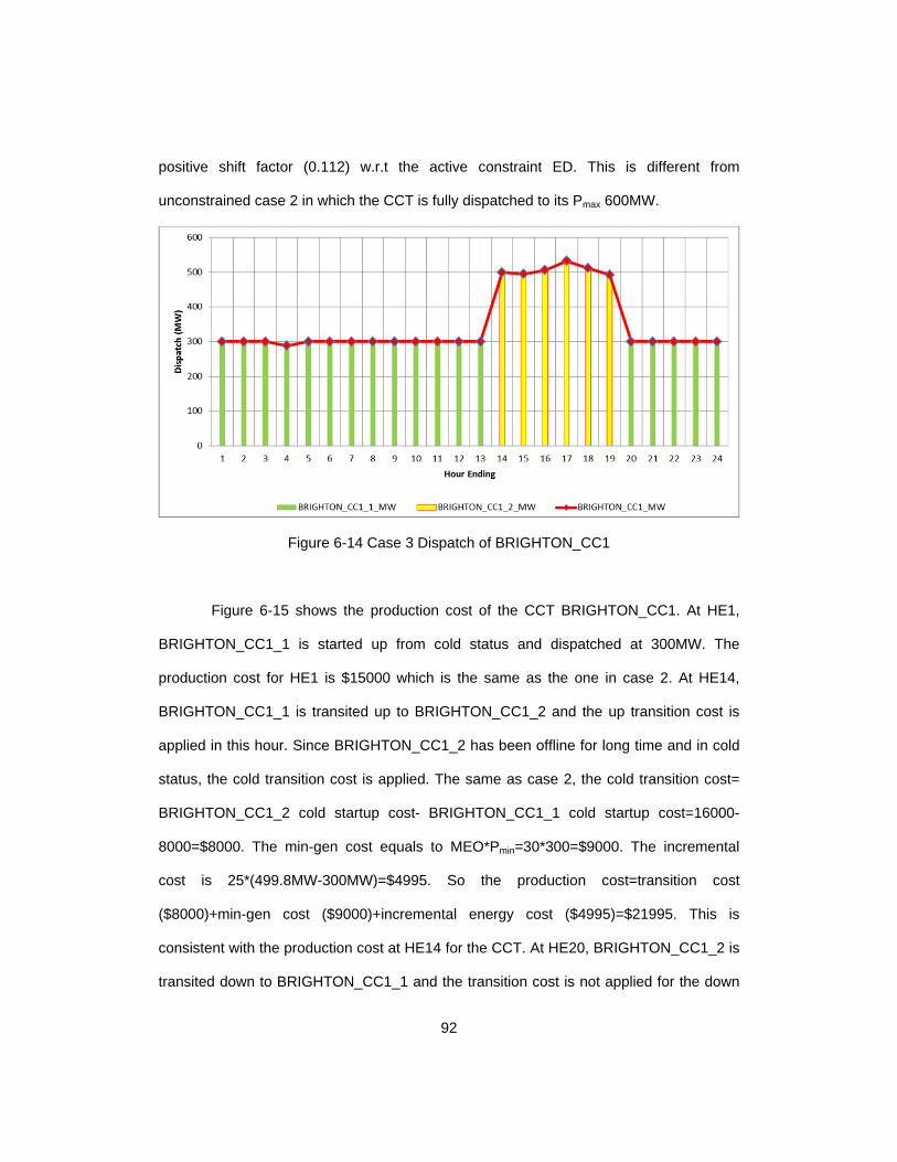
92
positive shift factor (0.112) w.r.t the active constraint ED. This is different from
unconstrained case 2 in which the CCT is fully dispatched to its Pmax 600MW.
Figure 6-14 Case 3 Dispatch of BRIGHTON_CC1
Figure 6-15 shows the production cost of the CCT BRIGHTON_CC1. At HE1,
BRIGHTON_CC1_1 is started up from cold status and dispatched at 300MW. The
production cost for HE1 is $15000 which is the same as the one in case 2. At HE14,
BRIGHTON_CC1_1 is transited up to BRIGHTON_CC1_2 and the up transition cost is
applied in this hour. Since BRIGHTON_CC1_2 has been offline for long time and in cold
status, the cold transition cost is applied. The same as case 2, the cold transition cost=
BRIGHTON_CC1_2 cold startup cost- BRIGHTON_CC1_1 cold startup cost=16000-
8000=$8000. The min-gen cost equals to MEO*Pmin=30*300=$9000. The incremental
cost is 25*(499.8MW-300MW)=$4995. So the production cost=transition cost
($8000)+min-gen cost ($9000)+incremental energy cost ($4995)=$21995. This is
consistent with the production cost at HE14 for the CCT. At HE20, BRIGHTON_CC1_2 is
transited down to BRIGHTON_CC1_1 and the transition cost is not applied for the down

93
transition in this hour. So the production cost=transition cost ($0)+min-gen cost
($3000)+incremental energy cost ($4000)=$7000. This is consistent with the production
cost at HE20 for the CCT shown in Figure 6-15.
Figure 6-15 Case 3 Production Cost of BRIGHTON_CC1
Figure 6-16 shows the LMP of CCT BRIGHTON_CC1 and system lambda for
each hour. One can see during HE14-HE19, the CCT LMP is equal to its incremental
energy cost and is less than the system lambda. This is because line ED is congested
during EH14-HE19 with non 0 shadow price and BRIGHTON_CC1 has a positive shift
factor w.r.t. line ED. Since LMP=system lambda-sum(shift factor*shadow price), the
calculated LMP is less than system lambda due to the positive shift factor. This is
consistent with the LMP in Figure 6-16. One also can see the BRIGHTON_CC1_2 is a
marginal unit satisfying the optimal condition during HE14-HE19: the LMP equals to its
incremental energy cost and the dispatch is greater than Pmin (300MW) and less than
Pmax (600MW).
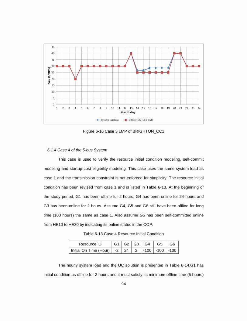
94
Figure 6-16 Case 3 LMP of BRIGHTON_CC1
6.1.4 Case 4 of the 5-bus System
This case is used to verify the resource initial condition modeling, self-commit
modeling and startup cost eligibility modeling. This case uses the same system load as
case 1 and the transmission constraint is not enforced for simplicity. The resource initial
condition has been revised from case 1 and is listed in Table 6-13. At the beginning of
the study period, G1 has been offline for 2 hours, G4 has been online for 24 hours and
G3 has been online for 2 hours. Assume G4, G5 and G6 still have been offline for long
time (100 hours) the same as case 1. Also assume G5 has been self-committed online
from HE10 to HE20 by indicating its online status in the COP.
Table 6-13 Case 4 Resource Initial Condition
Resource ID G1 G2 G3 G4 G5 G6
Initial On Time (Hour) -2 24 2 -100 -100 -100
The hourly system load and the UC solution is presented in Table 6-14.G1 has
initial condition as offline for 2 hours and it must satisfy its minimum offline time (5 hours)

95
to be committed by RUC. One can see G1 is offline during HE1-HE3 to meet its min
offline time even it is more economical than other resources. G2 has initial condition as
online 24 hours so the startup cost should not be applied if RUC commits it at HE1. One
can see that G2 has been committed for HE1-HE24 due to its low price. The production
cost for G2 at HE1 equals to min-gen cost (10*20) + incremental energy cost (15*(100-
10))=200+1350=$1550. This is consistent with the G2 production cost shown in Table
6-14. G3 has initial condition as online for 2 hours. Based on the self-commitment logic, if
the resource self-commitment can violate the temporal constraint and RUC shall not
commit unit just to meet unit self-commitment temporal constraint unless it is economic to
do so. In this case, G3 has high cost so it is not committed during HE1-HE8 even the
startup cost can be 0 if the unit is committed at HE1. This verifies that the self-
commitment logic is working as expected.
Figure 6-17 shows the hourly system load and system lambda for the 24 hour
study period.
Figure 6-17 Case 4 System Load and System Lambda

96
Table 6-14 Case 4 Hourly System Load and UC Solution
HE 1 2 3 4 5 6 7 8 9 10 11 12 13 14 15 16 17 18 19 20 21 22 23 24
Load 350 300 250 200 250 300 400 500 550 600 650 700 750 800 850 875 900 800 700 600 550 500 450 400
SL 20 20 20 14 15 15 20 20 20 30 30 30 30 30 30 30 30 30 30 30 20 20 20 20
Unit 1 2 3 4 5 6 7 8 9 10 11 12 13 14 15 16 17 18 19 20 21 22 23 24
G1 0 0 0 1 1 1 1 1 1 1 1 1 1 1 1 1 1 1 1 1 1 1 1 1
G2 1 1 1 1 1 1 1 1 1 1 1 1 1 1 1 1 1 1 1 1 1 1 1 1
G3 0 0 0 0 0 0 0 0 1 1 1 1 1 1 1 1 1 1 1 1 1 0 0 0
G4 0 0 0 0 0 0 0 0 0 0 0 0 0 0 0 0 0 0 0 0 0 0 0 0
G5 1 1 1 1 1 1 1 1 1 1 1 1 1 1 1 1 1 1 1 1 1 1 1 1
G6 0 0 0 0 0 0 0 0 0 0 0 0 0 0 0 0 0 0 0 0 0 0 0 0
Total 2 2 2 3 3 3 3 3 4 4 4 4 4 4 4 4 4 4 4 4 4 3 3 3
Unit 1 2 3 4 5 6 7 8 9 10 11 12 13 14 15 16 17 18 19 20 21 22 23 24
G1 0 0 0 90 110 110 110 110 110 110 110 110 110 110 110 110 110 110 110 110 110 110 110 110
G2 100 100 100 10 40 90 100 100 100 100 100 100 100 100 100 100 100 100 100 100 100 100 100 100
G3 0 0 0 0 0 0 0 0 52 90 140 190 240 290 340 365 390 290 190 90 52 0 0 0
G4 0 0 0 0 0 0 0 0 0 0 0 0 0 0 0 0 0 0 0 0 0 0 0 0
G5 250 200 150 100 100 100 190 290 288 300 300 300 300 300 300 300 300 300 300 300 288 290 240 190
G6 0 0 0 0 0 0 0 0 0 0 0 0 0 0 0 0 0 0 0 0 0 0 0 0
Total 350 300 250 200 250 300 400 500 550 600 650 700 750 800 850 875 900 800 700 600 550 500 450 400
Unit 1 2 3 4 5 6 7 8 9 10 11 12 13 14 15 16 17 18 19 20 21 22 23 24
G1 0 0 0 2326 1606 1606 1606 1606 1606 1606 1606 1606 1606 1606 1606 1606 1606 1606 1606 1606 1606 1606 1606 1606
G2 1550 1550 1550 200 650 1400 1550 1550 1550 1550 1550 1550 1550 1550 1550 1550 1550 1550 1550 1550 1550 1550 1550 1550
G3 0 0 0 0 0 0 0 0 6080 3220 4720 6220 7720 9220 10720 11470 12220 9220 6220 3220 2080 0 0 0
G4 0 0 0 0 0 0 0 0 0 0 0 0 0 0 0 0 0 0 0 0 0 0 0 0
G5 6000 5000 4000 3000 3000 3000 4800 6800 6760 4000 4000 4000 4000 4000 4000 4000 4000 4000 4000 4000 6760 6800 5800 4800
G6 0 0 0 0 0 0 0 0 0 0 0 0 0 0 0 0 0 0 0 0 0 0 0 0
Total 7550 6550 5550 5526 5256 6006 7956 9956 15996 10376 11876 13376 14876 16376 17876 18626 19376 16376 13376 10376 11996 9956 8956 7956
System Load (MW) and System Lambda ($/MWh) for Each Hour
Resource Commitment Status for Each Hour
Resource Dispatch (MW) for Each Hour
Resource Production Cost ($) for Each Hour
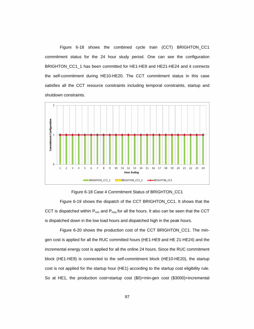
97
Figure 6-18 shows the combined cycle train (CCT) BRIGHTON_CC1
commitment status for the 24 hour study period. One can see the configuration
BRIGHTON_CC1_1 has been committed for HE1-HE9 and HE21-HE24 and it connects
the self-commitment during HE10-HE20. The CCT commitment status in this case
satisfies all the CCT resource constraints including temporal constraints, startup and
shutdown constraints.
Figure 6-18 Case 4 Commitment Status of BRIGHTON_CC1
Figure 6-19 shows the dispatch of the CCT BRIGHTON_CC1. It shows that the
CCT is dispatched within Pmin and Pmax for all the hours. It also can be seen that the CCT
is dispatched down in the low load hours and dispatched high in the peak hours.
Figure 6-20 shows the production cost of the CCT BRIGHTON_CC1. The min-
gen cost is applied for all the RUC committed hours (HE1-HE9 and HE 21-HE24) and the
incremental energy cost is applied for all the online 24 hours. Since the RUC commitment
block (HE1-HE9) is connected to the self-commitment block (HE10-HE20), the startup
cost is not applied for the startup hour (HE1) according to the startup cost eligibility rule.
So at HE1, the production cost=startup cost ($0)+min-gen cost ($3000)+incremental

98
energy cost ($3000)=$6000. This is consistent with the CCT production cost at HE1
shown in Figure 6-20. During HE2-HE6, BRIGHTON_CC1_1 is dispatched at Pmin
(100MW) so the production cost =min-gen cost=$3000. During HE10-HE20,
BRIGHTON_CC1_1 is self-committed so the production cost=incremental energy
cost=(300-100)*20=$4000. During HE21-HE24, the CCT is RUC committed and the
production cost=min-gen cost+ incremental energy cost.
Figure 6-19 Case 4 Dispatch of BRIGHTON_CC1
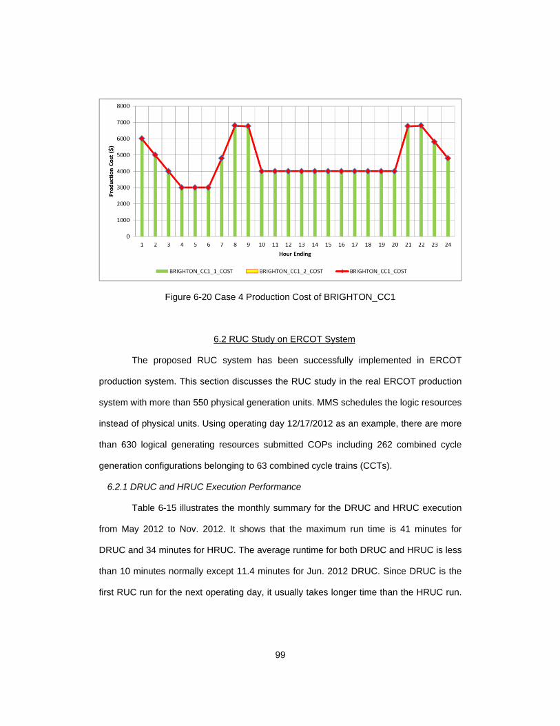
99
Figure 6-20 Case 4 Production Cost of BRIGHTON_CC1
6.2 RUC Study on ERCOT System
The proposed RUC system has been successfully implemented in ERCOT
production system. This section discusses the RUC study in the real ERCOT production
system with more than 550 physical generation units. MMS schedules the logic resources
instead of physical units. Using operating day 12/17/2012 as an example, there are more
than 630 logical generating resources submitted COPs including 262 combined cycle
generation configurations belonging to 63 combined cycle trains (CCTs).
6.2.1 DRUC and HRUC Execution Performance
Table 6-15 illustrates the monthly summary for the DRUC and HRUC execution
from May 2012 to Nov. 2012. It shows that the maximum run time is 41 minutes for
DRUC and 34 minutes for HRUC. The average runtime for both DRUC and HRUC is less
than 10 minutes normally except 11.4 minutes for Jun. 2012 DRUC. Since DRUC is the
first RUC run for the next operating day, it usually takes longer time than the HRUC run.

100
The execution summary for the seven months demonstrates that the performance for
both DRUC and HRUC is well within the runtime requirement.
Table 6-15 DRUC and HRUC Execution Monthly Summary
Month DRUC Execution HRUC Execution
Execution count
RuntimeAvg (min)
RuntimeMax (min)
Executioncount
RuntimeAvg (min)
Runtime Max (min)
May-12 31 7.2 18 744 6.2 17
Jun-12 29 11.4 41 719 7.2 19
Jul-12 31 7.4 35 744 6.2 20
Aug-12 31 6.8 26 744 6.5 24
Sep-12 30 6.3 16 720 6.7 22
Oct-12 31 9.0 31 744 7.8 31
Nov-12 30 7.8 29 721 6.9 34
To compare the nodal DRUC execution performance with the zonal RPRS, the
execution monthly summary of RPRS is shown in Table 6-16.
Table 6-16 Zonal RPRS Execution Monthly Summary
Month Execution
Count Runtime
Avg (min) Runtime
Max (min)
May-10 31 38.4 56.82
Jun-10 30 37.5 64.9
Jul-10 31 34.2 52.12
Aug-10 31 41.8 61.55
Sep-10 30 35.5 49.95
Oct-10 31 33.4 44.4
Nov-10 30 34.7 45.97
It can be observed that the DRUC average execution time is much less than the
average execution time for RPRS for each of the 7 months which demonstrates that the
RUC clearing process has higher performance than the RPRS process. The primary
reason is because that the RUC clearing and modeling logic is more advanced compared

101
to RPRS. The hardware upgrade and CPLEX solver improvement may also contribute to
the higher performance to some extent.
6.2.2 ERCOT RUC Study
Figure 6-21 shows the DRUC hourly scheduling summary for operating day
10/30/2012. The Self Scheduled HASL/HSL/LSL/LASL indicates the system total QSE
self-scheduled HSL/HASL/LSL/LASL calculated based on the COP of online resources.
The RUC Load Forecast is the net load requirement calculated as the sum of MTLF and
DC Tie Load. The Real-time Load is the real-time actual load from EMS telemetry. It can
be observed that the RUC Load Forecast is overall close to the Real-time Load with
some small errors. The RUC Recommended HSL is the output of the RUC optimization
which is calculated as the sum of HSL of both self-committed units and RUC committed
units. The RUC Recommended HSL will equal to the Self Scheduled HSL if there is no
RUC commitment for the specific hour.
As we can see in Figure 6-21, the Self Scheduled HASL is less than the RUC
Load Forecast at HE17, HE18 and HE20 which indicates that additional capacity need to
be committed to meet the load forecast by reserving the ancillary services limits. As
expected in this case, the RUC Recommended HSL is higher than the Self Scheduled
HSL indicating additional offline capacity has been committed.

102
Figure 6-21 DRUC Schedule Summary for 10/30/2012
Figure 6-22 shows the DRUC hourly schedule summary by resource type for
operating day 10/30/2012. The resource schedules (a.k.a. RUC clearing) are used to
project the congestion pattern in the RUC optimization. It can be observed that resource
type NUC (nuclear), CLLIG (coal) and CCGT90 (combined cycle greater than 90 MW)
are base load units and take up most of the total generation. It should be noted that the
RUC clearing results can be quite different from the real-time SCED clearing in some
cases. One possible reason is that RUC uses the proxy energy offer curve instead of
actual energy offer curve for RUC clearing. The proxy energy offer curve is calculated by
multiplying the mitigated offer cap curves with a very small discount factor. This approach
will make sure to dispatch low cost self-committed units first before commit offline units.
However it may result in different generation pattern in RUC compared to real-time
SCED.

103
Figure 6-22 DRUC Schedule Summary by Resource Type for 10/30/2012
Figure 6-23 demonstrates the DRUC average monthly schedule for Oct. 2012. It
can be observed that the RUC Load Forecast is very close to the Real-time Load. The
RUC Recommended HSL is also very close to the Self Scheduled HSL indicating minimal
RUC commitment for this month. This is reasonable because that the Self Scheduled
HASL is well above the RUC Load Forecast which means that there is more available
capacity margin for RUC dispatch.
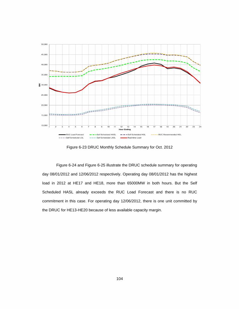
104
Figure 6-23 DRUC Monthly Schedule Summary for Oct. 2012
Figure 6-24 and Figure 6-25 illustrate the DRUC schedule summary for operating
day 08/01/2012 and 12/06/2012 respectively. Operating day 08/01/2012 has the highest
load in 2012 at HE17 and HE18, more than 65000MW in both hours. But the Self
Scheduled HASL already exceeds the RUC Load Forecast and there is no RUC
commitment in this case. For operating day 12/06/2012, there is one unit committed by
the DRUC for HE13-HE20 because of less available capacity margin.

105
Figure 6-24 DRUC Schedule Summary for 08/01/2012
Figure 6-25 DRUC Schedule Summary for 12/06/2012
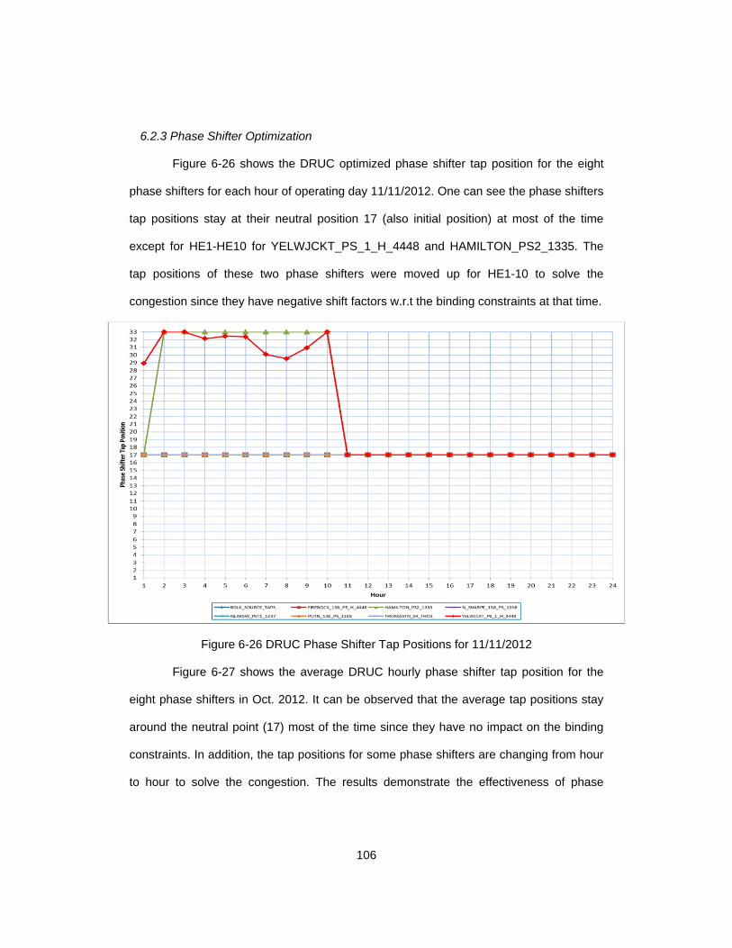
106
6.2.3 Phase Shifter Optimization
Figure 6-26 shows the DRUC optimized phase shifter tap position for the eight
phase shifters for each hour of operating day 11/11/2012. One can see the phase shifters
tap positions stay at their neutral position 17 (also initial position) at most of the time
except for HE1-HE10 for YELWJCKT_PS_1_H_4448 and HAMILTON_PS2_1335. The
tap positions of these two phase shifters were moved up for HE1-10 to solve the
congestion since they have negative shift factors w.r.t the binding constraints at that time.
Figure 6-26 DRUC Phase Shifter Tap Positions for 11/11/2012
Figure 6-27 shows the average DRUC hourly phase shifter tap position for the
eight phase shifters in Oct. 2012. It can be observed that the average tap positions stay
around the neutral point (17) most of the time since they have no impact on the binding
constraints. In addition, the tap positions for some phase shifters are changing from hour
to hour to solve the congestion. The results demonstrate the effectiveness of phase

107
shifter optimization, i.e. the phase shifters should stay at their initial/neutral tap positions
unless they are needed to solve transmission congestion.
Figure 6-27 DRUC Average Phase Shifter Tap Positions

108
Chapter 7
Conclusion and Recommendation for Future Studies
7.1 Conclusion
The case study and test results have demonstrated the benefit and effectiveness
of the proposed RUC modeling especially for the combined cycle unit (CCU) modeling.
During the design phase of the RUC project, a prototype RUC program was developed
with the proposed CCU modeling to verify the effectiveness of the CCU modeling. The
prototype RUC program has been tested on a revised PJM 5-bus system and the results
are very promising. Because of the positive testing results, the proposed CCU modeling
has been adopted for the RUC project and eventually has been implemented for the
production RUC. The testing results from the production RUC have demonstrated the
proposed RUC system is very robust and can improve dispatch efficiency and system
reliability as well as ensuring more effective congestion management.
The proposed RUC modeling has solved many challenges and deficiencies
identified in zonal RPRS market and greatly improved dispatch efficiency and system
reliability. The contribution of this research can be summarized as follows:
The proposed single step and NCUC-NSM iterative clearing process improves the
accuracy and efficiency of unit dispatch and congestion management.
The proposed two steps (UC and ED) NCUC solution algorithm decomposes the
complex MIQP problem into MIP and QP step and solves them sequentially. This
approach can enhance the solution performance without sacrificing accuracy.
The proposed configuration based combined cycle unit (CCU) modeling represents
the CCT more accurately and efficiently. The configuration-based model is more
adequate for bid/offer processing and dispatch scheduling and therefore it is adopted

109
in the NCUC. On the other hand, the physical unit modeling is more adequate for the
power flow and network security analysis and therefore it is adopted in the NSM.
The proposed phase shifter optimization utilizing the power injection model (PIM) can
solve congestion more efficiently in an automatic manner which can improve market
efficiency and improve system reliability.
The proposed offline time dependent startup cost modeling can represent the startup
cost more accurately and improve market efficiency.
The proposed ancillary service (AS) capacity modeling can protect the resource
specific AS capacity from dispatching unless the reservation leads to unresolved
transmission constraints. This approach reduces the AS undeliverable problem and
improves the system security.
7.2 Recommendation for Future Studies
More study can be performed to verify the benefit and effectiveness of the
proposed RUC modeling.
The rapid increase of wind energy in ERCOT and the characteristic that wind
power is far less predictable than system load, it imposes big challenges to system
operation. Future study should be done to better handle wind generation in RUC.
The incremental energy cost is discounted in RUC optimization to minimize the
RUC commitment. This may cause dispatch inconsistency and different congestion
pattern between RUC and real-time SCED. Further study can be performed to determine
a good balance between RUC commitment and dispatch.
The proposed SCUC framework can be extended to include the ramp rate
modeling to consider the ramp constraint between each interval of the study period. The

110
SCUC framework can also be adapted for the real-time commitment (RTC) which is used
to commit quick start units close to real-time.
The RUC discussed in this dissertation is a deterministic UC problem. To better
manage the uncertainties in UC, future research can be extended to stochastic unit
commitment and robust unit commitment.

111
Appendix A
Notation

112
Indices:
i Index for generating units.
s Index for phase shifters.
t Index for hours.
c Index for transmission constraints.
cc Index for combined cycle trains.
jou Index of jointly owned unit
p Index of startup cost segment
Variables:
,i tU On-line status indicator of unit i at interval t .
,cc tU On-line status indicator of combined cycle train cc at interval t .
,i tSU Startup indicator of unit i at interval t .
,i tSD Shutdown indicator of unit i at interval t .
, ,i t pISU Status indicator of startup cost segment p of unit i at interval t .
,i tP Dispatch MW of unit i at interval t .
,el tSlack Slack variable of energy long at interval t .
,es tSlack Slack variable of energy short at interval t .
,lc tSlack Slack variable of line constraint at interval t .
,s tPSCOST Cost function of phase shifter s at interval t .
,s tPST Tap position of phase shifter s at interval t .
,i tSUC Startup cost of unit i at interval t .
,i tMEC Minimum-energy cost of unit i at interval t .

113
,i tC Incremental energy cost of unit i at interval t .
Parameters:
psC Cost of moving phase shifter by 1 tap position.
NG Number of units.
NPS Number of phase shifters.
T Number of intervals in the study period.
0 ,s tPST Initial tap position of phase shifter s at interval t .
pbPenalty Penalty cost of power balance violation.
lcPenalty Penalty cost of line constraint violation.
tD Net system load at interval t .
,ci tSF Shift factor of unit i w.r.t. constraint c at interval t .
,cs tSF Shift factor of phase shifter s w.r.t. constraint c at interval t .
,MathLimit
c tF Mathematic limit of transmission constraint c at interval t .
min,i tP Minimum generating capacity of unit i at interval t .
max,i tP Maximum generating capacity of unit i at interval t .
JOU Set of physical jointly owned units
jouJOUGEN Set of logical unit of physical jointly owned unit jou .
iMNUP Minimum up time of unit i .
iMNDN Minimum down time of unit i .
iMXSU Maximum startup times of unit i .
,PhysicalLimit
c tF Physical limit of constraint c .

114
,NCUC
c tf Actual flow of constraint c .in NCUC.
0
,NSM
c tf Actual flow of constraint c .from previous NSM iteration.
,NCUCMath
c tf Mathematic flow of constraint c in NCUC.
,MathLimit
c tF Mathematic limit of constraint c in NCUC.
neutralsPST Neutral position of phase shifter s .
0,n tNCV Non-controllable variable, i.e. load in RUC.
,offset
c tF DC linearization offset (error) of constraint c .
,off
i pT Offline time corresponding to the startup cost segment p of unit i .
,i tNP Number of startup cost segment of unit at interval t .
,p
i tSUC Startup cost at segment p of unit i at interval t .
,i tMEO Minimum energy offer ($/MWh) of unit i at interval t .
ccCCGR Set of configurations of combined cycle train cc .
ccCCFT Set of feasible transition of CCT cc (FROM_CONFIG, TO_CONFIG).
ccCCIT Set of infeasible transition of CCT cc (FROM_CONFIG, TO_CONFIG).
ccCCGRSU Set of configurations which can be started up of CCT cc .
ccCCGRSD Set of configurations which can be shutdown of CCT cc .

115
Appendix B
Acronyms

116
AS ancillary service
CCGR combined cycle generation resource
CCT combined cycle train
CCU combined cycle unit
CMZ congestion management zone
COP current operating plan
CREZ competitive renewable energy zone
CRR congestion revenue right
CSC commercially significant constraint
CT combustion turbine
DAM day-ahead market
DRUC day-ahead reliability unit commitment
DC Tie direct current tie
ERCOT Electric Reliability Council of Texas, Inc.
EMS Energy Management System
HASL high ancillary service limit
HE hour ending
HEL high emergency limit
HRSG heat recovery steam generator
HRUC hourly reliability unit commitment
HSL high sustained limit

117
IRC ISO/RTO Council
ISO independent system operator
IUC initial unit commitment
JOU jointly owned unit
KV Kilovolt
LASL low ancillary service limit
LDF load distribution factors
LEL low emergency limit
LMP locational marginal price
LR Lagrangian relaxation
LSL low sustained limit
MIP mixed integer programing
MIQP mixed integer quadratic programming
MMS market management system
MOI market operator interface
MTLF mid-term load forecast
MW megawatt
MWh megawatt hour
NCUC network constrained unit commitment
NMMS network model management system
Non-Spin non-spinning reserve service

118
NSA network security analysis
NSM network security monitor
PIM power injection model
PSU pseudo unit modeling
PUCT Public Utility Commission of Texas
QF qualifying facility
QP quadratic programming
QSE qualified scheduling entity
RAP remedial action plan
RARF resource asset registration form
Reg-Down regulation down service
Reg-Up regulation up service
RMR reliability must-run
RPP renewable production potential
RPRS replacement reserve service
RRS responsive reserve service
RTCA real-time contingency analysis
RTC real-time commitment
RTO regional transmission organizations
RUC reliability unit commitment
SCADA supervisory control and data acquisition
SCED security constrained economic dispatch

119
SCUC security constrained unit commitment
SE state estimator
SGR split generation resource
SPS special protection scheme
ST steam turbine
STWPF short-term wind power forecast
TEWPF total ERCOT wind power forecast
UC unit commitment
WGR wind-powered generation resource
WGRPP wind-powered generation resource production potential
WRUC weekly reliability unit commitment

120
References
[1] IRC. [Online]. Available: http://www.isorto.org.
[2] “ERCOT Quick Facts,” [Online]: http://www.ercot.com/news/presentations/index
[3] ERCOT, “Brochure-Understanding Nodal,” [Online]: http://nodal.ercot.com-
/about/kd/understandingNodal012308.pdf
[4] ERCOT Training, [Online]: http://www.ercot.com/services/training/
[5] “ERCOT Nodal Protocols,” ERCOT, Taylor, TX. [Online]. Available:
http://www.ercot.com/mktrules/nprotocols.
[6] H. Hui, B. Whittle, C.-N. Yu et al. “MMS Reliability Unit Commitment (RUC)
Requirements”, ERCOT, Taylor, TX. [Online]. Available: http://nodal.ercot.com-
/docs/pd/mms/index.html#req.
[7] A. J. Wood and B. F. Wollenberg, Power Generation, Operation, and Control, 2nd
edition. New York: Wiley, 1996.
[8] B. F.Hobbs, M. H. Rothkopf, R. P. O’Neill and H. Chao, The Next Generation of
Electric Power Unit Commitment Models, New York: Kluwer Academic Publishers,
2002.
[9] M. Shahidehpour, H. Yamin, and Z. Li, Market Operations in Electric Power
Systems: Forecasting, Scheduling, and Risk Management. Piscataway, NJ: IEEE-
Wiley-Interscience, 2002.
[10] S. Stoft, Power Systems Economics: Designing Markets for Electricity. Piscataway,
NJ: IEEE Press/Wiley, 2002.
[11] J. A. Momoh, Electric Power Applications of Optimization, New York: Marcel Dekker,
2001.
[12] R. Fourer, D. M. Gay, and B. W. Kernighan, AMPL: A Modeling Language for
Mathematical Programming, 2nd edition. Duxbury Press, 2002.
121
[13] A. I. Cohen, V. Brandwajn, S.K. Chang, “Security Constrained unit Commitment for
Open Markets,” Proceedings of PICA Conference, pp. 39-44. May, 1999.
[14] Z. Li and M. Shahidehpour, “Security-Constrained Unit Commitment for
Simultaneous Clearing of Energy and Ancillary Services Markets,” IEEE Trans.
Power Syst., vol. 20, no. 2, pp.1079-1088, May 2005.
[15] H. Pinto, F. Magnago, S. Brignone, O. Alsac, and B. Stott, “security constrained unit
commitment: Network Modeling and Solution Issues”, IEEE Power Systems
Conference and Exposition, pp. 1759-1766, 2006.
[16] Y. Fu, M. Shahidehpour, and Z. Li, “Security-Constrained Unit Commitment With AC
Constraints”, IEEE Trans. Power Syst., vol. 20, no. 2, pp. 1538 - 1550, May 2005.
[17] Y. Fu and M. Shahidehpour, “Fast SCUC for Large-Scale Power System”, IEEE
Trans. Power Syst., vol. 22, no. 4, pp.2144 - 2151, Nov. 2007.
[18] L. Wu, M. Shahidehpour and T. Li, “Stochastic Security-Constrained Unit
Commitment,” IEEE Trans. Power Syst., vol. 22, pp.800-811, May. 2007.
[19] L. Wu, M. Shahidehpour, and T. Li, “Cost of Reliability Analysis Based on Stochastic
Unit Commitment,” IEEE Trans. Power Syst., Vol. 23, No. 3, pp. 1364–1374, Aug.
2008.
[20] B. Whittle, J. Yu, S. Teng, and J. Mickey, “Reliability Unit Commitment in ERCOT,”
Proceedings of IEEE PES General Meeting, Montreal, Canada, Jun. 2006.
[21] D. Sun, “Technical Challenges with Reliability Unit Commitment,” Proceedings of
IEEE PES General Meeting, Montreal, Canada, Jun 2006.
[22] A. Papalexopoulos, “Theoretical and practical considerations in implementing and
using a reliability unit commitment (RUC) in restructured electricity markets,”
Proceedings of IEEE PES General Meeting, Montreal, Canada, Jun 2006.

122
[23] R. Jones, “Midwest ISO Experience with Reliability Unit Commitment,” Proceedings
of IEEE PES General Meeting, Montreal, Canada, Jun 2006.
[24] A. Cohen and C.-N. Yu, “Unit Commitment in Energy Markets: Recent Experience
and Future Directions”, FERC Technical Conference on Unit Commitment Software,
Washington, DC, Jun. 2010.
[25] A. Ott, “Unit Commitment in the PJM Day-ahead and Real-time Markets,” FERC
Technical Conference on Unit Commitment Software, Washington, DC, Jun. 2010.
[26] M. Rothleder, “Unit Commitment at the CAISO,” FERC Technical Conference on
Unit Commitment Software, Washington, DC, Jun. 2010.
[27] R. Mukerji, “NYISO Day-Ahead Market Overview,” FERC Technical Conference on
Unit Commitment Software, Washington, DC, Jun. 2010.
[28] J. Wang, A. Botterud, J. Valenzuela and etc., “Stochastic Unit Commitment
Modeling: Implementation and Market Implications”, FERC Technical Conference on
Unit Commitment Software, Washington, DC, Jun. 2010.
[29] J. Zhao, T. Zheng and E. Litvinov, “Enhancing Reliability Unit Commitment with
Robust Optimization”, FERC Technical Conference on Unit Commitment Software,
Washington, DC, Jun. 2010.
[30] H. Hui, C.-N. Yu and S. Moorty, “Reliability Unit Commitment in the New ERCOT
Nodal Electricity Market,” Proceedings of IEEE PES General Meeting, Calgary,
Canada, July 2009.
[31] H. Hui, C.-N. Yu, F. Gao and R. Surendran, “Combined Cycle Resource Scheduling
in ERCOT Nodal Market,” Proceedings of IEEE PES General Meeting, Minneapolis,
MN, July 2011.
123
[32] H. Hui, C.-N. Yu, R. Surendran, F. Gao and S. Moorty, “Wind Generation
Scheduling and Coordination in ERCOT Nodal Market,” Proceedings of IEEE PES
General Meeting, San Diego, CA, July 2012.
[33] H. Hui, C.-N. Yu, R. Surendran, F.Gao, S. Moorty and X. Xu, “Look Ahead to the
Unforeseen: ERCOT’s Non-binding Look-Ahead SCED Study,” submitted for
Proceedings of IEEE PES General Meeting, Vancouver, Canada, July 2013.
[34] A. I. Cohen, and G. Ostrowski, “Scheduling Units with Multiple Operating Modes in
Unit Commitment,” IEEE Trans. Power Systems, Vol. 11, No. 11, pp. 497-503,
February. 1996.
[35] C. Liu, M. Shahidehpour, Z. Li and M. Fotuhi-Firuzabad, “Component and Mode
Models for the Short-Term Scheduling of Combined-Cycle Units,” IEEE
Transactions on Power systems, Vol. 24, No. 2, May 2009.
[36] G. Anders (Principal Investigator), “Commitment Techniques for Combined Cycle
Generating Units,” Kinectrics Inc, Toronto, Canada, December 2005.
[37] “Enhanced Day-Ahead Commitment Combined-Cycle Model,” IESO, Toronto
Canada, August 2008.
[38] “Modeling of Multi-Stage Generating Units,” CAISO. [Online] Available
http://www.caiso.com/2358/2358e27f11070.pdf.
[39] F. Gao and G. Sheble, “Economic Dispatch Algorithms for Thermal Unit System
Involving Combined Cycle Units, “ in Proc. 15th Power Systems Computation Conf.
2005, pp. 1-6, Session 21, Paper 5.
[40] M. Smith, “Combined Cycle Modeling in MRTU – The Challenges,” Calpine, Nov
2008. [Online] Available: http://www.caiso.com/208a/208a78f6301b0.pdf
[41] “IDA 003 White Paper: Combined Cycle Unit Modeling in the Nodal Design,”
ERCOT, Taylor TX.

124
[42] “ERCOT Nodal 101 Wind Generation,” ERCOT Nodal Training Team, Taylor, TX.
[43] S.-H. Huang, D. Maggio, K. McIntyre, V. Betanabhatla, J. Dumas and J. Adams,
“Impact of Wind Generation on System Operations in the Deregulated Environment:
ERCOT Experience,” Proceedings of IEEE PES General Meeting, Calgary, Canada,
Jun. 2009.
[44] C. D’Annunzio, S. Huang, and S. Santoso, “Generation Adequacy Assessment of
Power Systems with Wind Generation: A System Operations Perspective,”
Proceedings of IEEE PES General Meeting, Calgary, Canada, Jun. 2009.
[45] “2011-2012 ERCOT Methodologies for Determining AS Requirements,” ERCOT,
Taylor, TX.
[46] W. Lasher, “Transmission Planning in the ERCOT Interconnection,” ERCOT, Taylor,
TX [Online]: http://www.ercot.com/content/news/presentations/2011/ERCOT%20-
Transmission%20Planning%20DOE%20EAC%2010-20-11.pdf.
[47] N. P. Padhy, “Unit commitment—A bibliographical survey,” IEEE Trans. Power
Syst., vol. 19, no. 2, pp. 1196–1205, May 2004.
[48] H. Y. Yamin, “Review on methods of generation scheduling in electric power
systems,” Elect. Power Syst. Res., vol. 69, no. 2–3, pp. 227–248, May 2004.
[49] K. Hara, M. Kimura, and N. Honda, “A method for planning economic unit
commitment and maintenance of thermal power systems,” IEEE Trans. Power App.
Syst., vol. PAS-85, pp. 427–436, May 1966.
[50] R. H. Kerr, J. L. Scheidt, A. J. Fontana, and J. K. Wiley, “Unit commitment,” IEEE
Trans. Power App. Syst., vol. PAS-85, pp. 417–421, May 1966.
[51] R. R. Shoults, S. K. Chang, S. Helmick, and W. M. Grady, “A practical approach to
unit commitment, economic dispatch and savings allocation for multiple-area pool

125
operation with import/export constraints,” IEEE Trans. Power App. Syst., vol. PAS-
99, pp. 625–635, Mar./Apr. 1980.
[52] F. N. Lee, “Short-term unit commitment—a new method,” IEEE Trans. Power Syst.,
vol. 3, pp. 421–428, May 1988.
[53] F. N. Lee, “The application of commitment utilization factor (CUF) to thermal unit
commitment,” IEEE Trans. Power Syst., vol. 6, pp. 691–698, May 1991.
[54] W. L. Snyder, H. D. Powell, and J. C. Rayburn, “Dynamic-programming approach to
unit commitment,” IEEE Trans. Power Syst., vol. 2, no. 2, pp. 339–350, May 1987.
[55] W. J. Hobbs, G. Hermon, S. Warner, and G. B. Sheblé, “An enhanced dynamic
programming approach for unit commitment,” IEEE Trans. Power Syst., vol. 3, no. 3,
pp. 1201–1205, Aug. 1988.
[56] Z. Ouyang and S. M. Shahidehpour, “An intelligent dynamic-programming for unit
commitment application,” IEEE Trans. Power Syst., vol. 6, no. 3, pp. 1203–1209,
Aug. 1991.
[57] A. Merlin and P. Sandrin, “A new method for unit commitment at Electricité de
France,” IEEE Trans. Power App. Syst., vol. PAS-102, no. 5, pp. 1218–1225, May
1983.
[58] F. Zhuang and F. D. Galiana, “Towards a more rigorous and practical unit
commitment by Lagrange relaxation,” IEEE Trans. Power Syst., vol. 3, no. 2, pp.
763–773, May 1988.
[59] S. Virmani, E. C. Adrian, K. Imhof, and S. Muhherjee, “Implementation of a
Lagrangian based unit commitment problem,” IEEE Trans. Power Syst., vol. 4, pp.
1373–1380, Nov. 1989.

126
[60] C. Wang and S. M. Shahidehpour, “Ramp-rate limits in unit commitment and
economic dispatch incorporating rotor fatigue effect,” IEEE Trans. Power Syst., vol.
9, no. 3, pp. 1539–1545, Aug. 1994.
[61] C. Wang and S. M. Shahidehpour, “Optimal generation scheduling with ramping
costs,” IEEE Trans. Power Syst., vol. 10, no. 1, pp. 60–67, Feb. 1995.
[62] A. J. Svoboda, C.-L. Tseng, C.-A. Li, and R. B. Johnson, “Short-term resource
scheduling with ramp constraints,” IEEE Trans. Power Syst., vol. 12, no. 1, pp. 77–
83, Feb. 1997.
[63] S.-Y. Lai and R. Baldick, “Unit commitment with ramp multipliers,” IEEE Trans.
Power Syst., vol. 14, no. 1, pp. 58–64, Feb. 1999.
[64] H. Ma and S. M. Shahidehpour, “Unit commitment with transmission security and
voltage constraints,” IEEE Trans. Power Syst., vol. 14, pp. 757–764, May 1999.
[65] W. Ongsakul and N. Petcharaks, “Unit commitment by enhanced adaptive
Lagrangian relaxation,” IEEE Trans. Power Syst., vol. 19, no. 1, pp. 620–628, Feb.
2004.
[66] T. S. Dillon, K. W. Edwin, H. D. Kochs, and R. J. Tand, “Integer programming
approach to the problem of optimal unit commitment with probabilistic reserve
determination,” IEEE Trans. Power App. Syst., vol. PAS-97, no. 6, pp. 2154–2166,
Nov./Dec. 1978.
[67] M. Carrión and J. M. Arroyo, “A Computationally Efficient Mixed-Integer Linear
Formulation for the Thermal Unit Commitment Problem,” IEEE Trans. Power Syst.,
vol. 21, no. 3, pp. 1371-1378, Aug. 2006.
[68] C. K. Simoglou, P. N. Biskas, and A. G. Bakirtzis, “Optimal Self-Scheduling of a
Thermal Producer in Short-Term Electricity Markets by MILP,” IEEE Trans. Power
Syst., vol. 25, no. 4, pp. 1965-1977, Nov. 2010.
127
[69] J. M. Arroyo and A. J. Conejo, “Optimal response of a thermal unit to an electricity
spot market,” IEEE Trans. Power Syst., vol. 15, no. 3, pp. 1098–1104, Aug. 2000.
[70] T. Li and M. Shahidehpour, “Price-based unit commitment: A case of Lagrangian
relaxation versus mixed-integer programming,” IEEE Trans. Power Syst., vol. 20,
no. 4, pp. 2015–2025, Nov. 2005.
[71] G. W. Chang, Y. D. Tsai, C. Y. Lai, and J. S. Chung, “A practical mixed integer
linear programming based approach for unit commitment,” in Proc. 2004 IEEE PES
General Meeting, vol. 1, pp. 221–225, Jun. 2004.
[72] M. Carrion and J. M. Arroyo, “A computationally efficient mixed integer linear
formulation for the thermal unit commitment problem,” IEEE Trans. Power Syst., vol.
21, no. 3, pp. 1371–1378, Aug. 2006.
[73] J. M. Arroyo and A. J. Conejo, “Optimal response of a power generator to energy,
AGC, and reserve pool-based markets,” IEEE Trans. Power Syst., vol. 17, no. 2, pp.
404–410, May 2002.
[74] S. de la Torre, J. M. Arroyo, A. J. Conejo, and J. Contreras, “Price maker self-
scheduling in a pool-based electricity market: A mixed integer LP approach,” IEEE
Trans. Power Syst., vol. 17, no. 4, pp. 1037–1042, Nov. 2002.
[75] F. Zhuang and F. D. Galiana, “Unit commitment by simulated annealing,” IEEE
Trans. Power Syst., vol. 5, no. 1, pp. 311–318, Feb. 1990.
[76] A. H. Mantawy, Y. L. Abdel-Magid, and S. Z. Selim, “A simulated annealing
algorithm for unit commitment,” IEEE Trans. Power Syst., vol. 13, no. 1, pp. 197–
204, Feb. 1998.
[77] G. K. Purushothama and L. Jenkins, “Simulated annealing with local search—A
hybrid algorithm for unit commitment,” IEEE Trans. Power Syst., vol. 18, no. 1, pp.
273–278, Feb. 2003.

128
[78] S. A. Kazarlis, A. G. Bakirtzis, and V. Petridis, “A genetic algorithm solution to the
unit commitment problem,” IEEE Trans. Power Syst., vol. 11, no. 1, pp. 83–92, Feb.
1996.
[79] K. A. Juste, H. Kita, E. Tanaka, and J. Hasegawa, “An evolutionary programming
solution to the unit commitment problem,” IEEE Trans. Power Syst., vol. 14, no. 4,
pp. 1452–1459, Nov. 1999.
[80] J. M. Arroyo and A. J. Conejo, “A parallel repair genetic algorithm to solve the unit
commitment problem,” IEEE Trans. Power Syst., vol. 17, no. 4, pp. 1216–1224,
Nov. 2002.
[81] I. G. Damousis, A. G. Bakirtzis, and P. S. Dokopoulos, “A solution to the unit
commitment problem using integer-coded genetic algorithm,” IEEE Trans. Power
Syst., vol. 19, no. 2, pp. 1165–1172, May 2004.
[82] X. Guan, Q. Zhai, and A. Papalexopoulos, “Optimization based methods for unit
commitment: Lagrangian relaxation versus general mixed integer programming,”
Proceedings of IEEE PES General Meeting, vol. 2, pp. 1095–1100, Jul. 2003.
[83] D. Streiffert, R. Philbrick and A. Ott, “A mixed integer programming solution for
market clearing and reliability analysis,” Proceedings of IEEE PES General Meeting,
vol. 3, pp. 2724-2731, Jun. 2005.
[84] IBM ILOG CPLEX Optimizer Website, 2013. [Online]. Available: http://www-
01.ibm.com/software/integration/optimization/cplex-optimizer/.
[85] GUROBI Optimization Website, 2013. [Online]. Available: http://www.gurobi.com/.
[86] LINDO Systems Website, 2013. [Online]. Available: http://www.lindo.com/.
[87] FICO Xpress Website, 2013. [Online]. Available: http://www.fico.com-
/en/Products/DMTools/xpress-overview/Pages/Xpress-Optimizer.aspx.

129
[88] PJM Training: Locational Marginal Pricing 101, 2013. [Online]. Available:
http://www.pjm.com/training/training-material.aspx.
[89] Z. X. Han, “ Phase shifter and power flow control,” IEEE Trans. Power App. Syst.,
vol. 101, pp. 3790-3795, Oct. 1982.
[90] S.-K. Chang, V. Brandwajn, A. I. Cohen, M. Marwali, R. Gonzales, J. Jia, A.
Hargrave, “Phase shifter optimization in security constrained scheduling
applications,” Proceedings of IEEE PES Summer Meeting, vol. 3, pp. 1278-1283,
Jul. 2002.

130
Biographical Information
Hailong Hui received his B.S. and M.S. in Electrical Engineering from Southeast
University, Nanjing, China in 1999 and 2002 respectively. Currently he is pursuing his
Ph.D. in Electrical Engineering at The University of Texas at Arlington. He has been
working at Electric Reliability Council of Texas (ERCOT), Taylor, Texas since 2005 and
currently is a Senior Market Design Analyst in Market Design and Analysis department at
ERCOT. He has been actively involved in design and implementation of ERCOT Nodal
Market Management System. He has been the business lead in the nodal reliability unit
commitment (RUC) project and is responsible for the design and delivery of the RUC
system. Recently he has been actively involved in the design and implementation of the
look-ahead security constrained economic dispatch (LA-SCED) project at ERCOT. His
research interests include electricity market, power system operation and optimization.


