Reliability-Based Design Optimization for Aerospace and Automotive Structures

Roberto d’Ippolito (roberto.dippolito@lms.be), Stijn Donders (stijn.donders@lms.be),Luc Hermans (luc.hermans@lms.be), Herman Van der Auweraer

(herman.vanderauweraer@lms.be)LMS International, Interleuvenlaan 68, B-3001 Leuven, Belgium

Dirk Vandepitte (dirk.vandepitte@mech.kuleuven.be)Katholieke Universiteit Leuven, Department of Mechanical Engineering, Division PMA,

Kasteelpark Arenberg 41, B-3001 Heverlee, Belgium

Abstract

The need for improvements in engineering designs especially for aerospace and automotive structures is nowadays becoming a major industry request. Deterministic approaches are unable to take into account all the variabilities that characterize design input properties without leading to oversized structures. This paper intends to give a description of the most commonly used methods for reliability based design optimization using the performance measure approach to point out the advantages of the application of this method in the design process. Furthermore, an outline of the methodology will be given that could serve as a guideline to develop a more efficient and optimized design process that takes into account the input parameters variability. For this purpose two Finite Element models have been created, one for an industrial composite wing structure and one for a vehicle knuckle. Realistic variability has been assigned to material properties and static load conditions. A range of analysis cases, with gradually increasing complexity, has then been defined. This allows the assessment of the reported methods in terms of accuracy, computation time and applicability in conjunction with Finite Element models.

1 INTRODUCTION

Currently, aerospace and automotive industries are dedicating a lot of attention to improve product quality and reliability already in a virtual simulation environment. The aerospace industry is nowadays using composite materials more and more for both aeronautic and space applications. This trend is shifting the traditional design paradigm dealing with metal structures to a modified paradigm involving hybrid metal/polymer structures. The new design process that is needed to build these structures requires also a shift from the traditional

design approach to a new approach that integrates all the variabilities and uncertainties that hybrid designs introduce, mainly due to the use of composite materials.

Also the automotive industry is facing new challenges, especially in the field of durability and reliability of structural components, in order to achieve better performances together with improved safety.

Unfortunately, current deterministic approaches are unable to take into account all the variabilities that characterize aerospace and automotive designs, without oversizing structures or assuming a too pessimistic view on the actual material properties and on the operating conditions.

Traditionally, safety factors have been applied to the product specifications and dimensions in order to make sure that the structure complies with the internal and external requirements, while being also robust to variability on the design parameters. Unfortunately, these safety factors are often rather arbitrary and typically overestimate the actual variability. This might result in a design with a much higher level of robustness than what is actually required. Especially for (composite) aerospace materials, this could lead to structures that are “heavier than needed”, thus producing too conservative designs that don’t fully exploit the real benefits that lightweight composite materials can bring to the aerospace design process.

A more promising approach is to include the property variability in the design flow and to use computer simulation methods to guarantee the design reliability. This paper gives a description of the most commonly used methods to improve the reliability of aerospace and automotive structures. Particularly, a Reliability-based Design Optimization (RBDO) procedure will be illustrated, that uses reliability methods not only to assess the reliability of a given design, but sets a step further: it allows computing a more reliable design for the given product variability.

When accurate stochastic descriptions of physical properties are available, these can be integrated into the design process of aerospace and automotive structures and a procedure management and optimization tool can be developed to• assess the inherent risk of the preliminary design• identify the most relevant parameters• optimize the structure to meet targets on structural

performance and safety

2 TEST CASES DESCRIPTION

For demonstration purposes, an aerospace and an automotive analysis projects have been created, to improve the reliability of a composite wing subject to gust loads and the reliability of a vehicle knuckle fatigue life, respectively. Finite Element (FE) models are used to represent these structures in a simulation environment and realistic variability has been assigned to material properties and static load conditions. The RBDO procedure has then been used to improve the design of these structures.

2.1 The composite wing

A static analysis is performed on a real prototype composite wing in order to optimize the structure for a high altitude, long endurance (HALE) unmanned air vehicle (UAV), for which the characteristics are briefly

summarized in Figure 1. The composite wing has been made of AS4 12k/3502 unitape. Many properties of this material have already been statistically characterized in the Military Handbook 17-2E and can therefore immediately be used in a probabilistic formulation . The considered input parameters are summarized in Table 1:

Property Distrib. Mean VarianceFiber E1 [Pa] Normal 1.3307•1011 7.6381•109

Fiber E2 [Pa] Normal 9.3079•109 3.9652•108

Fiber G12 [Pa] Normal 3.7438•109 1.9318•108

Density [Kg/m3] Normal 1575 2.5Stringer Fiber E1 [Pa] Normal 1.3307•1011 7.6381•109

Table 1. Statistically characterized material properties at 75º F (23.89º C)

In this paper, all the input variables are considered to be statistically independent. Unfortunately this

approximation is not always true in reality because the realistic characterization of the correlation coefficients is often very difficult and therefore considered impractical for most engineering applications.

The composite wing has been examined under gust load conditions, with the wing clamped in the section that connects to the fuselage as boundary condition. The Pratt formula has been used to evaluate the gust load. To characterize a worst-case scenario, a stronger gust situation is considered for most of the presented structural analyses. To stiffen the structure, stringers are distributed over the entire wing. They are considered as one-dimensional elements in the FE model, so only the fiber modulus along the fiber direction has been used (Stringer E1, SE1).

As stated before, a Finite Element model of the wing has been created to perform the analysis and a particular framework for the necessary computations has been set up. More details on the analysis implementation are given in section 4.1.

2.2 The vehicle knuckle

To demonstrate the advantages of the probabilistic methodology applied to fatigue cases, a typical automotive analysis case is considered as well. The vehicle lifetime is highly determined by the fatigue life of its components; in turn, variability in material properties may affect the fatigue life. This is demonstrated for the

vehicle knuckle structure shown in Figure 2. The structure is made of steel, and has properties (with inherent variabilities) as specified in Table 2. A fatigue analysis is performed based on a validated FE model; the aim is to increase the fatigue life in the presence of variability.

Figure 1. Main composite wing characteristics and geometry

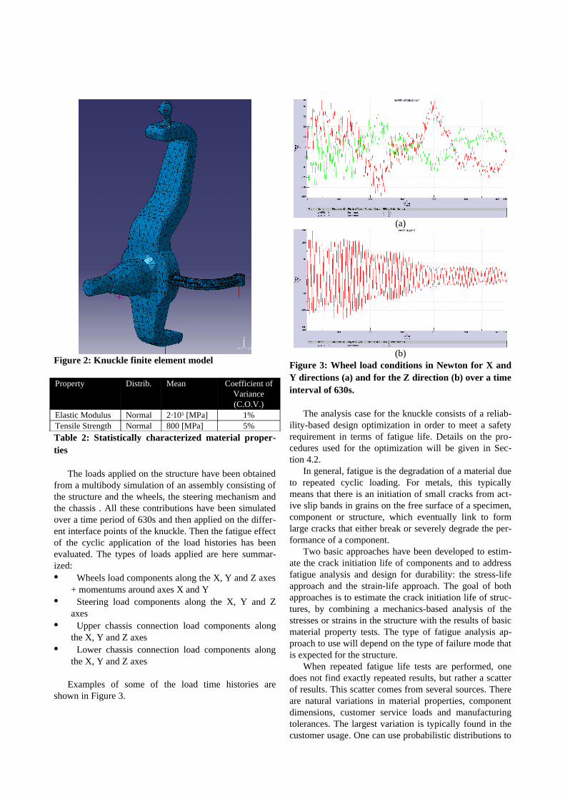
Figure 2: Knuckle finite element model

Property Distrib. Mean Coefficient ofVariance(C.O.V.)

Elastic Modulus Normal 2·105 [MPa] 1%Tensile Strength Normal 800 [MPa] 5%

Table 2: Statistically characterized material proper-ties

The loads applied on the structure have been obtained from a multibody simulation of an assembly consisting of the structure and the wheels, the steering mechanism and the chassis . All these contributions have been simulated over a time period of 630s and then applied on the differ-ent interface points of the knuckle. Then the fatigue effect of the cyclic application of the load histories has been evaluated. The types of loads applied are here summar-ized:• Wheels load components along the X, Y and Z axes

+ momentums around axes X and Y• Steering load components along the X, Y and Z

axes• Upper chassis connection load components along

the X, Y and Z axes• Lower chassis connection load components along

the X, Y and Z axes

Examples of some of the load time histories are shown in Figure 3.

(a)

(b)Figure 3: Wheel load conditions in Newton for X and Y directions (a) and for the Z direction (b) over a time interval of 630s.

The analysis case for the knuckle consists of a reliab-ility-based design optimization in order to meet a safety requirement in terms of fatigue life. Details on the pro-cedures used for the optimization will be given in Sec-tion 4.2.

In general, fatigue is the degradation of a material due to repeated cyclic loading. For metals, this typically means that there is an initiation of small cracks from act-ive slip bands in grains on the free surface of a specimen, component or structure, which eventually link to form large cracks that either break or severely degrade the per-formance of a component.

Two basic approaches have been developed to estim-ate the crack initiation life of components and to address fatigue analysis and design for durability: the stress-life approach and the strain-life approach. The goal of both approaches is to estimate the crack initiation life of struc-tures, by combining a mechanics-based analysis of the stresses or strains in the structure with the results of basic material property tests. The type of fatigue analysis ap-proach to use will depend on the type of failure mode that is expected for the structure.

When repeated fatigue life tests are performed, one does not find exactly repeated results, but rather a scatter of results. This scatter comes from several sources. There are natural variations in material properties, component dimensions, customer service loads and manufacturing tolerances. The largest variation is typically found in the customer usage. One can use probabilistic distributions to

characterize the variation of these variables, and include this variability in the design process to better explain and predict the scatter obtained in fatigue test results. Probab-ilistic methods offer a powerful tool to assess the inherent risk of designs for durability through the characterization of the inherent variabilities, by allowing the design engin-eer to minimize the weight and costs requirements, without losing reliability with respect to durability re-quirements.

3 THE RELIABILITY PROBLEM STATEMENT

As stated in Section 1, the variabilities of an engineering design can be characterized by the variations of a random system parameter set

[ ] nixx Ti ...1with ==

The probability distribution of each xi is described either by its cumulative distribution function

(CDF, ( )ix xFi ) or by its probability density function

(PDF, ( )ix xfi ) and is often bounded by tolerance limits

on the system parameter values.The system performance is described by Performance

Functions (PF, ( ) mjxGj ...1with = ) that, for a structur-

al design, are usually the selected failure criteria. Thus,

with ( )xGj one of the m system PFs, the system is con-

sidered to fail if ( ) 0<xGj for at least one index j. The

probability of failure of the system for every jth perform-ance function is then

( ) ( )( ) ( )∫ ∫Ω

=<=j

j nXjG dxdxxfxGPF 100(1)

where ( ) 0:: <ℜ∈Ω xGx jn

j

The event space jΩ is the region of the stochastic

space where only failure events occur. Thus, the integral of the joint probability density function of the system re-

sponse over jΩ yields the probability of failure jfP , of

the structure for the jth criterion. In general, given a fixed

performance index (or measure) jg of the system, Eq (1)

can be generalized

( ) ( )( ) ( )∫ ∫Ω

=<=jG

j nXjjjG dxdxxfgxGPgF 1 (2)

where ( ) jjn

G gxGxj

<ℜ∈Ω ::

In this case, the event space jGΩ represents the re-

gion of the stochastic space where the performance of the

structure is below a prescribed quantity jg .

3.1 The Reliability-Based Design Optimization (RBDO) Model

In engineering design, the traditional deterministic design optimization model has been successfully applied to sys-tematically improve the system design process, yielding a reduction of the costs and an improvement of the final quality of the products. However, uncertainties in either engineering simulations and/or manufacturing processes exist. This calls for different optimization models that can yield not only an improvement in the design, but also a higher level of confidence. Thus, a reliability-based design optimization (RBDO) model for robust and cost-effective designs can be defined using mean values of the random system parameters as design variables and optim-izing the cost subject to prescribed probabilistic con-straints (e.g. a maximum on the allowed probability of failure) by solving a mathematically nonlinear program-ming problem. As a result, the RBDO solution provides not only an improved design but also a higher level of confidence in the design.

The general RBDO model can be defined as

( )[ ]( )( )

=≤<= mjPxGPP

dCost

jfjjf

d

1 with 0 s.t.

min

,,(3)

where the cost function can be any function of the design

variable [ ] [ ]TiT

idd µ≡= and a probabilistic constraint

jfP , can be defined for each failure mode. Thus, for each

iteration of the optimization loop, an estimation of the probabilistic constraint has to be computed. For this pur-pose, different methods exist. In general, each prescribed

probability of failure jfP , can be represented in terms of

the target reliability index jt,β as

( ) ( )jtjfjfjt PP ,,,1

, ββ −Φ=⇒Φ−= − (4)

also defined by the more general relation

( ) ( )( ) ( )jj GjjjG gxGPgF β−Φ=<= (5)

where ( )•Φ is the standard normal CDF (zero mean and standard deviation 1).

Using Eq. (5), the second condition of Eq. (3) can be rewritten as

( ) ( ) ( )jtjs

jfjtjsGjf PFPj

,,

,,,, 0

ββ

ββ

≥⇒

=−Φ≤−Φ==(6)

where js,β is traditionally called “reliability index” of the

structure for the specified failure mode j. Through inverse transformations, Eq (6) can be written as

( )( ) 0,1* ≥−Φ= −

jtGj jFg β (7)

where *jg is named “target probabilistic performance

measure” and represents the value of the performance

function “equivalent” to the target reliability index jt,β .

3.2 Performance Measure Approach

The formulation of the general RBDO model of Eq. (3) that uses Eq. (6) to describe the probabilistic constraint is called Reliability Index Approach (RIA) . An alternative and more effective way of formulating the general RBDO model is to use the inverse formulation of the probabilist-ic constraint of Eq. (7), known as Performance Measure Approach (PMA) . The RBDO model can be re-written as

( )[ ]( )( )

=≥−Φ= − mjFg

dCost

jtGj

d

j1 with 0 s.t.

min

,1* β

(8)

In this case, at a given design [ ] [ ]Tki

Tki

k dd )()()( µ≡= ,

the evaluation of the target probabilistic performance

measure *jg is performed using

( ) ( )

= ∫ ∫

Ω

−

jG

j nXGk

j dxdxxfFdg 11)(* (9)

For each iteration of the optimization process the fol-lowing problem has to be solved

( )[ ]

=

=

t,j

ju

u

mjuG

s.t.

1 with min (10)

The approximate solution of this problem yields an estimation of the performance measure, given by

( )**, jt

uGg j ββ =≈ (11)

With this formulation, the performance measure *jg ,

which depends on the design points, has to be estimated within each iteration and the target of the optimization is to find the design point that can satisfy all the probabilist-ic constraints in terms of the performance measure. This approach yields an improved convergence rate of the PMA methodology with respect to the RIA formulation. In fact, PMA minimizes a complex cost function subject to a simple constraint, which gives rise to less numerical problems and therefore a better algorithm performance, while the RIA algorithm minimizes a simple cost function subject to a complex constraint.

3.3 Limit State Approximations (LSA)

In most industrial cases, the integral of Eq. (9) cannot be evaluated in closed form. Only for simple academic cases, fX can be defined analytically. In such a case, the

performance function ( )xGj for each specific failure

mode of the structure is available so that jΩ can be

defined. The boundary of the domain jΩ is also called

limit-state surface and the function ( )xGj is called the

limit-state function (LSF) .In the most widely used reliability method, approxim-

ations are made in the space of standard uncorrelated nor-mal variates, Y, obtained from a transformation of the ba-sic variables

( )XTY = (12)

where the transformation T is expressed in terms of the distributions of X.

For the sake of simplicity, only the case with one fail-ure criterion (j=1) will be considered in this paper. There-fore, from here on, the j index is removed from all the quantities that depend on j.

In the space Y, denoted as the standard normal space,

approximations of the probability of failure jfP , of

Eq. (3) are obtained by replacing the limit state surface with first or second order approximating surfaces. These surfaces are fitted to the limit state surface at points with minimal distance to the origin (design points).

3.4 First and Second Order Reliability Methods

In the first order reliability method (FORM), the limit state surface is approximated by its tangent hyperplane in the standard normal space Y at the global minimum dis-tance point (Most Probable Point, MPP) on the limit state function. With this approximation, the reliability index

s coincides with the distance of the MPP to the ori-

gin. In the second order reliability method (SORM) the limit state surface is approximated by a paraboloid, defined with the same principal curvatures as estimated for the limit state surface at the design point (MPP). De-termination of these curvatures essentially requires com-puting the second-order derivative matrix of the limit state surface and solving an associated eigenvalues prob-lem.

The determination of the MPP involves the solution of the following constrained optimization problem:

( )( )

YyyGts

yyyf T

y ∈

=

=

with0..2

1min

(13)

To achieve the optimal solution, the Karush-Kuhn-Tucker (KKT) conditions have to be satisfied. For only one equality constraint, the Lagrangian expression and the KKT conditions can be reduced to:

( ) ( ) ( )yGyfyL λλ +=, (14)

( )

==∇

0)(

0,*

**

yG

yLy λ(15)

where (y*, *) is the solution point.Many algorithms are available in literature to solve

this problem, usually combining a direction search al-gorithm and a line search procedure along that direction. A well-established algorithm for the reliability index ap-proach (RIA) is the modified HL-RF algorithm. For the Performance Measure Approach (PMA), the Hybrid Mean Value (HMV) scheme exhibits good performance.

Although they are well established and widely used, LSA approximations such as FORM and SORM exhibit some limitations when the degree of nonlinearity in the LSF increases. Since the FORM approach is a linear ap-proximation, it is easy to understand that it ignores all nonlinearities in the LSF. Furthermore, as the number of dimensions of the problem increases, also the error of the approximation for all LSAs increases accordingly, without the possibility to estimate it within the same reli-ability calculation (“curse of dimensionality”). In prac-tice, this means that for problems with a number of di-mensions n>15, special care should be paid to the degree of nonlinearity of the performance function(s) because the error of the approximation strongly depends on this nonlinearity.

4 ANALYSIS CASES IMPLEMENTATION

In order to perform the analysis the methodology reported in Section 3.2 has been implemented in a MATLAB code and used to perform the analysis. The Optimization process is managed by an OPTIMUS thread (Figure 4

and upper part of Figure 6) that determines the necessary steps to reach the optimum design point that satisfies the probabilistic constraint of Eq. (16). The optimization al-gorithm selected for all the analysis cases is the Sequen-tial Quadratic Programming (SQP) using a tolerance of 10-3 and forward finite difference gradient estimation. Note that the optimization process is a deterministic pro-cess with a probabilistic constraint. Thus the result is an optimum point that is also robust with respect to the re-quired failure probability.

4.1 The composite wing

For the composite wing structure proposed in Section 2.1, a Finite Element model has been created and the external load configuration has been applied. With the variability introduced in the input parameters, the performance beha-vior of the FE model has been observed and the RBDO process reported in Section 3 has been applied to meet the following probabilistic constraint:

-109.866 =⇒= ft Pβ (16)

Figure 4. OPTIMUS project for Reliability-based Design Optimization process

Figure 5. OPTIMUS project for Process automationFor each iteration of the optimization process, the al-

gorithm requires the evaluation of the performance func-tion at specific values of the input parameters, so that a FE static analysis (for the present case the Nastran solver has been used) has to be performed for each evaluation. To accomplish this task, another process management thread (Figure 5) using OPTIMUS has been created: when the MATLAB algorithm (for the estimation of the performance measure) requires a performance function evaluation for a given parameter vector, OPTIMUS launches a FE computation and submits the results back to MATLAB, where the LSF criterion is evaluated.

4.2 The vehicle knuckle

For the testcase proposed in Section 2.1, a similar proced-ure has been applied to optimize the fatigue life response of the knuckle FE model.

Due to the computational effort required for each fa-tigue life evaluation, a hybrid meta-model/FE strategy has been used. In fact, a full factorial, multi-level Design of Experiments (DOE) plan has been designed in order to explore the fatigue life response within the boundaries of interest. Subsequently, a quadratic Response Surface (RS) model has been computed based on the DOE results. The obtained meta-model has then been used for a first RBDO process using a PMA methodology.

The DOE strategy used to build the meta-model starts with a full factorial, 3 levels design, in the range [-3 , +3 ] . The DOE plan has then been expan-ded to a 5 levels design in the range [-6 , +6 ] and then up to a 7 levels design in the range [-9 , +9 ] . This choice has been made to better explore the possible nonlinear behavior of the fatigue life response and to validate the meta-model on a wider inter-val of analysis. Thus a total of 49 experiments have been run and the maximum absolute error of the meta-model showed to be less than 0.1 when compared with FE simu-lation results.

The outline of the procedure used for the analysis is

1. Compute the response of the structure with 3 DOE plans

a. Compute the 3 levels DOE plan in the range [-3 +3 ]

b. Compute the 5 levels DOE plan in the range [-6 +6 ] , re-using previous step results

c. Compute the 7 levels DOE plan in the range [-9 +9 ] , re-using previous step results

2. Compute the quadratic least squares response model RS (using Taylor Approximation)

3. Perform an RBDO loop using the RS model and obtain a first tentative optimum point

4. Validate (and refine if needed) the results of the previous step with FE computations.

The implementation of the analysis for the vehicle knuckle differs from the previous one in the process auto-mation loop. In fact, in order to evaluate the performance function at specific values of the input parameters, a se-quence of FE static analysis and LMS FALANCS fatigue analysis has to be performed for each evaluation.

The probabilistic constraint set for the RBDO process is:

-109.866 =⇒= ft Pβ (17)

This means that the design optimum will be a 6 design w.r.t. the PF selected in Section 5.

MATLAB Algorithms (HL-RF, HMV)

OPTIMUS Optimization Loop

OPTIMUS Process Integration

Figure 6: Optimization loop and Process Integration with MATLAB and OPTIMUS

As in the previous implementation, the optimization process is managed by an OPTIMUS thread (as shown in Figure 6) that determines the necessary steps to reach the optimum design point that satisfies the probabilistic con-straint of Eq. (17).

5 PERFORMANCE FUNCTION CHOICE

The selection of a proper performance function is a key task in the reliability analysis process. Of course it is strongly case dependent and even for the same structure, it can change depending on the particular aspect that has to be analyzed. In this section, a description of the specif-ic performance function selection for the two analysis cases is reported.

5.1 The Composite Wing

As the wing considered in this paper consists entirely of composite material, a special failure criterion should be chosen. The majority of failure criteria for composite ma-terials are based on energetic theories, but few of them, like the Tsai-Wu criterion, have been developed and tested for industrial composite applications. It is common convention to consider that the composite structure breaks when one of its constituents breaks, as until now there are no criteria that take into account the presence of residual stress in the laminate. In the case considered in this paper for the composite wing, the Tsai-Hill failure criterion, derived from the more general Hill criterion for anisotropic materials, has been used as performance func-tion. This criterion is defined by the following formula:

+

+−

−=

2

12

122

2

22

1

212

1

11FFFF

Gσσσσσ

(18)

The maximum Tsai-Hill index over all the plies of all laminates (i.e. a first-ply failure criterion) represents the performance of the structure. An example of the resulting multidimensional surface, given the input parameter vari-ability, is represented in Figure 7: the displayed values belong to a section of the multidimensional space refer-ring to the main hyper-planes passing through the origin. To prevent having to deal with an infinite design space, the transformed standard normal space is bounded in a hyper-cube between –10 and +10 and the optimization range for each variable is between –4 and +4 with respect to the nominal starting value (these are the initial mean values of the parameters exhibiting variability). As can be seen in Figure 7, the surface is quite flat around the nominal values of the design para-meters and becomes quite steep (w.r.t. the scatter around the nominal value) when approaching the LSF.

-10 -5 0 5 10-10

-5

0

5

10

E2

E1

-10-50510

-10

0

10

-2

0

2

4

x 108

E2

E1

LSF

LSF

(a) (b)Figure 7. Contour plot of the Limit State Function in the transformed space

Four analysis sub-cases have been designed, using either the input variability in Table 1 or the nominal values. The sub-cases follow the description given in Table 3.In this paper, only material properties have been con-sidered. Note however that the methodology is not lim-ited to this class of parameters as similar analyses can be performed for geometrical or strength properties. The in-creasing number of parameters in the sub-case sequence in Table 3 will be used to show how the addition of new parameters influences the results of the optimization pro-cedure (and the corresponding reliability index for each iteration).

5.2 Vehicle Knuckle

Before discussing the choice of the performance function for the present case, some observations are needed. Vari-ous failure modes exist in durability cases, and the identi-fication of the failure mode is important in both testing and analysis. Testing at load levels that are too high will change the failure mode and give the incorrect safety factors or may identify incorrect critical locations. The failure modes here considered are• A static (non-fatigue) failure mode: this results in

large structural deformation and is controlled primarily by the resistance of the net section.

• Low cycle fatigue: this is usually the result of a large plastic zone at a notch, or stress concentration. Low cycle fatigue behavior depends on the notch severity and the inelastic material response.

• High cycle fatigue: this is representative of a situation in which there is little plasticity. Here the notch severity, manufacturing processes and residual stresses play an important role.

For fatigue analysis, the strain-life approach is typic-ally used in situations where yielding of the material may be present at certain locations on the structure. This ap-proach has been developed based on knowledge of more detailed material behavior when subjected to stress levels above the yield strength of the material. On the contrary, the stress-life approach is typically more suitable in situ-ations where the stresses are below (or not much above) the elastic limit of the material.

Following the previous considerations, the choice of the performance function is related to the Maximum Damage sustained by the structure. For this case, a Max-imum Damage value of –1 (in log10 scale) has been selec-ted. The performance function can than be written as

( )10

1

1

−<>⇒⇒+−=⇒

⇒−=

MaxDamageforG

MaxDamageG

MaxDamage

(19)

With this choice, the G function is positive where MaxDamage is less than –1, which is in agreement with the definition of the reliability problem reported in Sec-tion 3.

In this paper, only material properties have been con-sidered. Note however that the methodology is not lim-ited to this class of parameters as similar analyses can be performed with variability in geometrical or strength properties, load conditions, … .

Testcase Variable 1 Variable 2 Variable 3 Variable 4 Variable 5

1Fiber E1 Fiber E2 Mean Fiber G12 Mean

(Rho)Mean Stringer E1

2Fiber E1 Fiber E2 Fiber G12 Mean

(Rho)Mean Stringer E1

3 Fiber E1 Fiber E2 Fiber G12 (Rho) Mean Stringer E1

4 Fiber E1 Fiber E2 Fiber G12 (Rho) Stringer E1

6 RESULTS

The results of the optimization processes for both the ana-lysis cases are reported in this section. The differences in the procedures and the influence on the results of the dif-ferent hypotheses are stressed.

6.1 Composite wing results

For the composite wing case, Table 4 shows the optimiza-tion results using PMA. The optimization process has been repeated for all 4 sub-cases, in order to demonstrate how the results may change by introducing additional variability. An indication of the total computational effort spent for each optimization procedure is given by the re-quired number of Limit State Function (LSF) evaluations: more computations means a higher computational effort.

SQPIteration

Performance Measure G(x)SC 1 SC 2 SC 3 SC 4

0 0.2514 0.2523 0.2523 -0.0441 0.1182 0.1252 0.1117 0.00462 0.0441 0.1242 0.1036 0.00253 -0.0034 0.0615 0.0695 -0.00094 0.0003 0.0163 0.021 -0.00055 0.0001 0.0054 -0.0108 0.00016 - 0.0049 0.0031 -7 - 0.0046 0.0023 -8 - 0.0033 - -

N. of LSF evaluations

630 2076 1775 3605

Table 4. Performance Measure estimation in the op-timization results for different testcases using PMA (results in the table are expressed in terms of perform-ance function value in the parameter space)

-10 -5 0 5 10-10

-8

-6

-4

-2

0

2

4

6

8

10

E1

E2

-10-5

05

10

-10-5

05

10

-2

-1

0

1

2

3

4x 10

8

E1

E2

GX

(a) (b)

Figure 8. Optimization process for sub-case 1 using PMA

A visualization of the optimization process for sub-case 1 is shown in Figure 8(a) and Figure 8(b).

For the other sub-cases, the optimum points are repor-ted in Table 5. It is shown that the position of the optim-um point is noticeably affected by the introduction of new random parameters. These random parameters are repres-entative of the variability of the input parameters and are described by probability distributions. As a result, while in the first sub-case Fiber E1 is decreased and Fiber E2 is increased, in sub-case 4 the opposite occurs.

-10 -5 0 5 10-10

-8

-6

-4

-2

0

2

4

6

8

10

Stringer E1

E2

-10 -5 0 5 10 -10

0

10

-10

-8

-6

-4

-2

0

2

Stringer E1

E2

GX

(a) (b)Figure 9. Optimization process for sub-case 4 and parameters E2 and Stringer E1

The introduction of the last parameter has a strong in-fluence on the position of the optimum point. This is due to the fact that the stringers are stiffening elements in the structure, thus variability in their properties influences the structure more than the variability in the 2nd, 3rd and 4th

parameter. This can clearly be observed in Figure 9 that plots the LSF for the 2nd and 5th parameter.

6.2 Vehicle knuckle results

Referring to the outline of the procedure reported in Sec-tion 4, different steps have been considered for the vehicle knuckle. Due to the higher computational effort required for each fatigue analysis, a design of experi-ments strategy has been used to assess the response of the structure with a limited number of evaluations . The first step consisted in the computation of the fatigue life (in terms of Maximum Damage) using 3 different DOE plans. Table 6 reports the values of the Maximum Dam-age for the 3, 5 and 7 levels DOE plans, as defined in Section 4.

Testcase Fiber E1 Fiber E2 Fiber G12

(Rho)Stringer E1

1 -1.0388 3.9200 Nominal Nominal Nominal2 -0.8677 4.0134 -1.3472 Nominal Nominal3 -0.7614 4 1.7929 4 Nominal4 0.31719 -0.3487 -0.03564 0.81411 1.7215

Table 5. Optimization results in standard normal space (Y-Space) using PMA

Using the results of the DOE plan of Table 6, a least squares quadratic Taylor Response Surface has been computed to approximate the FE model. A plot of the re-sponse surface is shown in Figure 10. The RS has an ab-solute maximum error of less than 0.1, thus can be used as meta-model in order to assess the reliability of the FE model and to compute the first part of the optimization

procedure.

-10

-5

0

5

10

-10-8 -6 -4

-2 0 24 6 8

10

-2.5

-2

-1.5

-1

-0.5

0

0.5

E

Tensile Strength

Max

imum

Dam

age

Figure 10: Response sur-face of the Maximum dam-age (log10 scale) as a func-tion of the Elastic modulus and Tensile Strength.

-10 -8 -6 -4 -2 0 2 4 6 8 10-10

-8

-6

-4

-2

0

2

4

6

8

10

TS

, Ten

sile

Str

engt

h

E, Elastic Modulus

STARTING POINT

OPTIMIZED POINT

Figure 11: RBDO pro-cedure using the PMA and the Hybrid Mean Value (HMV) al-gorithm.

Apparently, the optimization procedure seems simple, as there’s only a single equality constraint to be formally satisfied (see Section 4). A closer look at the problem re-veals that the optimization loop should in fact meet two optimization objectives: the first is the equality constraint and the second is that the newly found design point should also minimize the Maximum Damage.

It’s easy to figure out that the solution locus for the first constraint is constituted by all the points at a distance of 6 from the LSF. But among these points, there is only one point that minimizes the Maximum Damage of the structure. Thus the multi-objective procedure should satisfy two constraints, one equality constraint and one inequality constraint:

( ) =

MaxDamaget

minimize

6β(20)

In order to meet both targets, the optimization proced-ure outlined in Section 4.2 has been implemented for an objective that is a combination of the two constraints of Eq. (20). The new objective can be expressed as:

( )MaxDamagetS −− ββmin (21)

Using this new objective, the optimization process has been carried out using the Performance Measure Ap-proach and the HMV algorithm , looking for a robust op-timum point in the range [-3 +3 ] for each parameter (i.e. E and TS). The results of the optimization are reported in Table 7 and Table 8 and shown in Figure11.

SQP IterationElastic Modulus

(MPa)Tensile Strength

(MPa)1 200000.00 800.002 200155.19 897.673 200277.41 905.784 200415.38 905.755 201100.98 905.386 204519.58 903.517 206000.00 902.79

Table 7: RBDO results using PMA

Number of SQP Iterations 7Number of LSF evaluations 240Time needed for completion 26 seconds

Table 8: RBDO performance using PMA

The optimized point found with the use of the re-sponse surface model has then been used as a starting point for a refinement optimization procedure involving only FE computations. Before stepping into the refine-ment process results, some considerations on the choice of using a Response Surface approximation are reported, to point out the advantages and disadvantages of this meta-modeling technique.

E \ TS↓ →[Mpa]

440

560 680 800 920 1040 1160

182000 0.0 -0.41494 -1.05 -1.4369 -1.6716 -1.8451 -1.9948188000 0.0 -0.42428 -1.0689 -1.4634 -1.7043 -1.8811 -2.033194000 0.0 -0.42778 -1.0885 -1.4879 -1.7315 -1.9122 -2.07200000 0.0 -0.43051 -1.1044 -1.5122 -1.7626 -1.9438 -2.1039206000 0.0 -0.43406 -1.12 -1.5342 -1.7892 -1.9737 -2.1356212000 0.0 -0.43653 -1.1369 -1.556 -1.8143 -2.0007 -2.1656218000 0.0 -0.43881 -1.1511 -1.5774 -1.8389 -2.0275 -2.1952

(in log10 scale) for the 7 levels DOE plan. Different colors show the 3 and 5 levels DOE plans.

6.3 Considerations on the Response Surface model

To better understand the differences between the Re-sponse Surface model and the FE computations, some rel-evant contours of the Maximum Damage values in the stochastic transformed space are presented. These con-tours have been computed with the FE model and with the DOE/RS model. Figure 12 compares a quadratic RS model with a contour based on a higher number of FE analyses than the DOE plans points. In the region where the behavior is quite linear, the accuracy of the terms with order higher than linear might not be sufficient. This gives rise to slight errors in the estimates with the RS model in this linear region. It can however be concluded that the RS model is a suitable first approximation model that can yield sufficiently accurate results with a very limited computational effort. Moreover, it saves many FE computations in the optimization process, by locating an initial point which is very close to the solution, so that the subsequent refinement process (that usually implies addi-tional FE computations) becomes much faster.

-10 -8 -6 -4 -2 0 2 4 6 8 10-10

-8

-6

-4

-2

0

2

4

6

8

10

TS

, T

ensi

le S

tren

gth

E1, Elastic Modulus

LIMIT STATE FUNCTION

-10 -8 -6 -4 -2 0 2 4 6 8 10-10

-8

-6

-4

-2

0

2

4

6

8

10

TS

, T

ensi

le S

tren

gth

E, Elastic Modulus

LIMIT STATE FUNCTION

(a) FE Computation (b) DOE/RS ModelFigure 12: Differences between the FE and the RS model.

6.4 Refinement of the RBDO results

The results of the refinement process using only FE com-putations are here reported. As it can be seen, even if the number of required optimization loops is less than the number required with the RS model, the time needed for the complete process to finish is some orders of mag-nitude greater. The results of the refinement process are reported in Table 9 and Table 10 and the comparison with the RS RBDO process in Table 11.

SQP IterationElastic Modulus

(MPa)Tensile Strength

(MPa)1 206000.00 902.582 206000.00 894.753 206000.00 894.23

Table 9: RBDO refinement results for the vehicle knuckle using PMA

Number of SQP Iterations 3Number of PF evaluations 289Time needed for completion 80920 seconds

(= 22h 28m 40s)

Table 10: FE RBDO refinement loop performance for the vehicle knuckle case using PMA

RS RBDO Time(seconds)

FE refinement RBDO Time(seconds)

Ratio(FE/RS)

26 80920 3112.3

Table 11: Performance comparison of the refinement process with the RS model first optimization loop.

The results obtained from the refinement process show that the RS model is indeed conservative. Figure 12 shows that the “real” LSF (in terms of FE computations) is located slightly further than the LSF of the RS model. This means that the optimum point found with the RS model is at a distance a little larger than 6 . However, the difference between the Tensile Strength (TS) of the RS model and the TS of the FE refinement is sufficiently small when compared to the standard devi-ation of the TS property. This means that the FE refine-ment process can be considered too expensive (in terms of computational time) w.r.t. the advantage it brings.

To conclude, it must be noted that the limited number of significant digits available in FE computations slows down the convergence of both the PMA iterations and the SQP optimizations. In order to limit this effect, a semi-adaptive step for the finite difference gradient estimation has been used.

7 CONCLUSIONS

In this paper, a composite wing and a vehicle knuckle have been analyzed under different load conditions and with variabilities in the input parameters. Several obser-vations have been made.

It has been shown that the methodology used to op-timize the presented structures enables the designer to reach a higher level of confidence in the reliability of the design performance in the presence of realistic variabilit-ies. The presented procedures are generally applicable and not limited to a specific engineering field. Moreover, the simplicity of integration in the design loop has been demonstrated in Section 4. Also different analysis strategies have been outlined, to demonstrate the flexibil-ity that these procedures have, as they take advantage of existing and well-known modeling techniques. Thus, the methodology outlined in this paper for the analysis of so different cases constitutes an effective general-purpose tool to assess the inherent risk of a design. It allows the design risk to be reduced in accordance with safety regu-lations, to gain advantages in costs and time-to-market. The major outcome of this analysis effort is a more robust and safe design.

For the specific applications considered in this paper, some other considerations arise. In particular, the effect of nonlinearities introduced by new variabilities in the in-put parameters should not be underestimated. One should carefully investigate what are the most relevant paramet-

ers to be included in the optimization loop through a pre-liminary assessment of the performance of the structure. For this purpose, one can use PMA. As an example, the results of the analysis of the composite wing are not only influenced by the probability that high- or low-quality materials are used, but also by the probability that a par-ticular combination of different panel and stringer materi-al properties occurs. Furthermore, it has been demon-strated that the dimensionality of the problem plays an important role as well. The introduction of the 5th para-meter variability drastically changes the configuration of the failure surface defined by the Tsai-Hill criterion.

In the case of more computational intensive analyses, a hybrid meta-model/FE approach can be used that proved to be effective to save analysis time and get an ac-curate result as well. In fact, the response surface model used for the first RBDO process in the analysis of the vehicle knuckle exhibits some conservatism w.r.t. the FE computations of the DOE plan, but can be successfully used to find a sufficiently accurate result. Therefore, the refinement process (using FE computations in place of the RS model) yields a small improvement in the solution that had been found with the RS RBDO procedure. Thus, the FE refinement can be considered to be not necessary if the RS model captures the behavior of the real FE mod-el with sufficient accuracy. In the majority of the cases, this applies for performance functions that don’t exhibit strongly non-linear behavior in the region where the re-sponse surface is defined.

8 ACKNOWLEDGMENTS

The presented methodologies are being studied and de-veloped in the context of the EC research training net-work (RTN) MADUSE (Modeling product vAriability and Data Uncertainty in Structural dynamics Engineer-ing), see http://www.maduse.org/, and the ongoing re-search project ‘Analysis Leads Design – Frontloading Di-gital Functional Performance Engineering’, which is sup-ported by IWT Vlaanderen. The support of the European Commission, of IWT and of the Marie Curie Fellowship Association is gratefully acknowledged.

9 REFERENCES

[1] MIL-HDBK-17, Polymer Matrix Composites, Volume 1, Guidelines, February 1992.

[2] Long, M.W.; Narciso, J.D.: Probabilistic Design Methodology for Composite Aircraft Structures, Final Report DOT/FAA/AR-99/2, June 1999.

[3] d’Ippolito, R.; Donders, S.; Tzannetakis, N.; Van der Auweraer, H., Vandepitte, D., Integration of Probabilistic Methodology in the Aerospace Design Optimization Process, 46th

AIAA/ASME/ASCE/AHS/ASC Structures, Structural Dynamics and Materials Conference, Austin, Texas, USA, Apr. 18-21, 2005, AIAA-2005-2137.

[4] LMS International, LMS Virtual.Lab, Rev. 5A, July 2005.

[5] Sudret, B.; Der Kiureghian, A.: Stochastic Finite Element Methods and Reliability, A state of the art report, Report N. UCB/SEMM-2000/08 Department of Civil and Environmental Engineering, University of California, Berkley, November 2000.

[6] Melchers, R.B.: Structural Reliability Analysis and Prediction, 2nd Edition, 1999.

[7] Youn, B.D.; Choi, K.K.; Park, Y.H.: Hybrid Analysis Method for Reliability-Based Design Optimization, Journal of Mechanical Design, vol 125, pp 221-232,

June 2003, ASME.

[8] Schuëller, G.I., Pradlwarter, H.J., Koutsourelakis, P.S., A Critical appraisal of reliability estimation procedures for high dimensions, Probabilistic Engineering Mechanics, Vol. 19, pp. 463-474, 2004.

[9] The MathWorks Inc., MATLAB Version 6.5, June 2002.

[10]Noesis Solutions, OPTIMUS Rev. 5.1, July 2005.

[11]MSC, MSC/NASTRAN 2001, February 2001.

[12]Barkey, M., Hack, M., Speckert, M., Zingsheim, F., FALANCS User Manual, Kaiserlautern, 1998.

[13]d’Ippolito, R., Donders, S., Tzannetakis, N., Van de Peer, J., Van der Auweraer, H., Design Improvements of composite aerospace structures using reliability analysis, Proc. IMAC XXIII, Orlando, Florida, USA, Jan. 31-Feb. 3, 2005.