Reliability Analysis Technique Comparison, as Applied … · · 2011-06-01Reliability Analysis...
45
Reliability Analysis Technique Comparison, as Applied to the Space Shuttle AE 8900 OLD – Special Topic By Alex Keisner December 5 th , 2003
Transcript of Reliability Analysis Technique Comparison, as Applied … · · 2011-06-01Reliability Analysis...

Reliability Analysis Technique Comparison, as Applied to the Space Shuttle
AE 8900 OLD – Special Topic
By Alex Keisner
December 5th, 2003

2
TABLE OF CONTENTS
1. Introduction………………………………………………………………………...…6 2. The Space Shuttle……………………………………………………………..............7 2.1 The Challenger Accident …………………………………………………………….10 2.2 The Columbia Accident………………………………………………………………12 2.3 Investigation Board Findings and Suggestions……………………………………...15 3. Reliability Analysis Techniques…………………………………………………….17 3.1 Qualitative Techniques……………………………………………………………...17 3.2 Quantitative Techniques……………………………………………………..............18 3.2.1 Fault Tree Analysis………………………………………………………………...19 3.2.2 Reliability Block Diagram…………………………………………………………20 3.2.3 Markov Analysis…………………………………………………………………...21 3.2.4 Petri Nets…………………………………………………………………………...23 4. Space Shuttle Analyses……………………………………………………………...26 4.1 SAIC Probabilistic Risk Assessment (PRA)…………………………………………26 4.2 Relex FTA……………………………………………………………………………28 4.3 BlockSim RBD……………………………………………………………………….34 5. Conclusions…………………………………………………………………………..38 Appendix A – Relex Fault Trees……………………………………………………….42 References……………………………………………………………………………….45

3
LIST OF FIGURES
Figure 2.1 – Launch of Apollo 11…………………………………………………………7 Figure 2.2 – Columbia during re-entry on STS-1…………………………………………9 Figure 2.3 – Challenger immediately after the explosion of the SRB…………………...12 Figure 2.4 – STS-107 being launched from KSC………………………………………..13 Figure 2.5 – Columbia starts breaking up upon re-entry………………………………...14 Figure 3.1 – Sample FTA………………………………………………………………...20 Figure 3.2 – Sample RBD of a series of two sets of two parallel gates………………….21 Figure 3.3 – Sample Markov Chain……………………………………………………...22 Figure 3.4 – Sample Petri Net……………………………………………………………24 Figure 4.1 – The top event and some subsequent high level events of the LOV PRA com-
pleted by SAIC………………………………...…………………………………27 Figure 4.1 – The top event and some subsequent high level events of the LOV PRA com-
pleted by SAIC…………………………………………………...………………29 Figure 4.3 – LOV Relex fault tree with added detail under LOV due to SSME………...30 Figure 4.4 – Plot of top event probability versus level of detail…………………………31 Figure 4.5 – Relex fault tree of LOV due to SSME……………………………………...32 Figure 4.6 – LOV due to SSME failure to maintain proper configuration portion of PRA
fault tree………………………………………………………………………….33 Figure 4.7 – LOV due to SSME failure to contain energetic gas and debris portion of…33 Figure 4.8 – Relex FTA of LOV due to APU failure to contain energetic gas and debris34 Figure 4.9 – All four parts of the PRA fault tree associated with APU hydrazine turbine
overspeed and hub failure………………………………………………………..34 Figure 4.10 – BlockSim RBD of three-level LOV………………………………………36 Figure 4.11 – BlockSim RBD of LOV due to SSME……………………………………36 Figure 4.12 – BlockSim RBD of APU hydrazine turbine overspeed and hub failure…...37 Figure 5.1 – Bridge structure RBD………………………………………………………38 Figure 5.2 – Necessary FTA of a bridge structure……………………………………….39

4
LIST OF TABLES
Table 3.1 – Comparison of Reliability Analysis Method Characteristics………………25
Table 4.1 – Comparison of Reliability Analysis Techniques……………….…………..37

5
LIST OF ACRONYMS
APU Auxiliary Power Unit
EAFB Edwards Air Force Base
ET External Tank
FMEA Failure Modes and Effects Analysis
FMECA Failure Modes, Effects, and Criticality Analysis
FTA Fault Tree Analysis
KSC Kennedy Space Center
LOV Loss of Vehicle
MEIDEX Mediterranean-Israeli Dust Experiment
NASA National Aeronautics and Space Agency
PRA Probabilistic Risk Assessment
RCC Reinforced Carbon-Carbon
RLV Reusable Launch Vehicle
SRB Solid Rocket Booster
SSME Space Shuttle Main Engine
STS Space Transportation System
TPS Thermal Protection System

6
1. Introduction
With the events of the Columbia Space Shuttle accident and all of the investigation and
speculation that followed, safety and reliability have become much more focused upon in
the space industry. To this day, even with technology growing and advancing as it has,
there has not been a single reliability analysis technique developed to perfectly model any
advanced system, especially a system as complex as the Space Shuttle. All methods cur-
rently used have many advantages, along with several faults inherent in each technique.
Within the reliability community there are several different methods that are used, and
there is no consensus of which is the best method to use. Even when determining the best
method, there are many criteria that could be used to make this distinction. Whether it be
the easiest to use, the most accurate to represent a complex model, the fastest computa-
tional tool, the most simplified method, or an array of other measures of which analysis is
“best”, there is no clear-cut favorite for most of these. The most widely used method of
reliability analysis within the Aerospace Engineering community is Fault Tree Analysis
(FTA), which is good for modeling complex systems in that it is a relatively simple
method. However, many say FTA is too simplified and unable to accurately model com-
plex systems for several reasons.1
7
2. The Space Shuttle
Human space flight began on April 12th, 1961, when cosmonaut Yuri Gagarin was
launched into orbit aboard the Vostok 1. This was accomplished in the midst of the space
race in which the former Soviet Union and the United States were constantly competing
and trying to better one another in the area of human space travel. The space race has
often been credited with helping to advance the technologies involved, and propel space
travel forward at an incredible rate that would not have been possible otherwise.
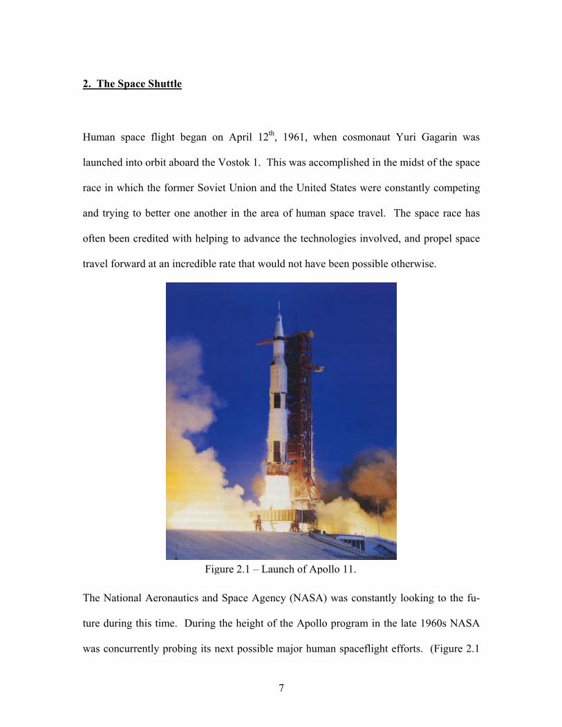
The National Aeronautics and Space Agency (NASA) was constantly looking to the fu-
ture during this time. During the height of the Apollo program in the late 1960s NASA
was concurrently probing its next possible major human spaceflight efforts. (Figure 2.1
Figure 2.1 – Launch of Apollo 11.

8
shows the launch of Apollo 11 aboard a Saturn V booster.) In January 1972, President
Richard Nixon declared that NASA would begin development of a Space Transportation
System (STS), more commonly known as the Space Shuttle.2
The idea behind the Space Shuttle was to provide relatively inexpensive, frequent access
to space through the use of a reusable launch vehicle (RLV). NASA had envisioned the
use of a fully reusable vehicle in order to keep the trip costs at a minimum, with visions
of space stations in orbit around the Earth, as well as in lunar orbit and eventually on the
lunar surface. When it was realized that these visions of future use and exploration were
infeasible, NASA aimed to justify the Space Shuttle on economic grounds, projecting that
through the combination of military, commercial, and scientific payloads, the Space Shut-
tle could be flown for 50 missions a year. However, many of the commitments made by
NASA during the policy process lead to a design aimed at satisfying many conflicting
requirements. The goals were a vehicle capable of carrying large payloads and cross-
range capability, but with low development costs and an even lower operating cost. The
result of all of this conflict within the design requirements has been a vehicle that is very
costly and difficult to operate, and is much riskier than was originally anticipated.3
Once completed, the Space Shuttle was subjected to a vast array of tests well before its
first flight. But unlike with the other spacecraft NASA had operated, the Space Shuttle
was tested much differently. The philosophy of the Space Shuttle Program was to
ground-test key hardware elements, such as the Solid Rocket Boosters (SRB), the Exter-
nal Tank (ET), the Orbiter, and the Space Shuttle Main Engines (SSME) separately.

9
Then analytical models were used to certify the integrate Space Shuttle System, as op-
posed to the flight testing that had been used with previous spacecrafts. Even though
crews verified that the Orbiter could successfully fly at low speed and land safely, the
Space Shuttle was not flown on an unmanned orbital test prior to its first mission, which
was contrary to the philosophy of earlier American spaceflight.4
The Space Shuttle also depended highly on significant advances in technology, which
cause the development to run well behind schedule. The original launch date for the
Shuttle’s first launch was in March of 1978, but due to many delays it was pushed back
several times, finally being set for April of 1981. An historian described the problems by
attributing one year of delays “to budget cuts, a second year to problems with the main
engines, and a third year to problems with the thermal protection system.”5 A review by
the White House was taken in order to ensure that the Space Shuttle was still worth con-
tinuing in 1979, but this need was reaffirmed and the door was now open to transition
from development to flight. In addition, despite the fact that only 24,000 of 30,000
Thermal Protection System (TPS) tiles had been attached, NASA decided to move Co-
Figure 2.2 – Columbia during re-entry on STS-1.

10
lumbia to the Kennedy Space Center (KSC) from the manufacturing plant in Palmdale
California in order to maintain the image that it would be capable of meeting its sched-
uled launch date.4
The first Space Shuttle mission, STS-1, was successfully launched on April 12, 1981, and
returned safely two days later to Edwards Air Force Base (EAFB) in California. It is
shown during its re-entry in Figure 2.2. The next 3 missions were all launched over the
following 15 months aboard the orbiter Columbia as well, undergoing extensive testing
and inspection following each one. At the end of its fourth mission, Columbia landed at
EAFB on July 4, 1982, where President Ronald Reagan declared that “beginning with the
next flight, the Columbia and her sister ships will be fully operational, ready to provide
economical and routine access to space for scientific exploration, commercial ventures,
and for tasks related to national security.”3 From 1982 to early 1986 the Space Shuttle
demonstrated its capabilities for space operations. It flew science missions with the
European-built Spacelab module in its payload bay, retrieved two communications satel-
lites that had suffered upper-stage misfires, and repaired another communications satellite
on-orbit. In 1985, between the four orbiters in use nine missions were launched, and by
the end of the year 24 communications satellites had been put into orbit, with a backlog
of 44 more orders for future commercial launches. Although it seemed to the public that
things were progressing well, the facts were that the system was much more difficult to
operate than expected, with more maintenance between flights than anticipated. Rather
than requiring the 10 working days projected in 1975, by the end of 1985 it was taking an
average of 67 days to process a returned Orbiter for its next flight.4

11
2.1 The Challenger Accident
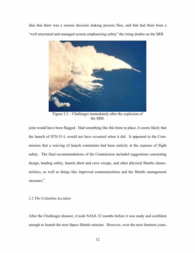
The image that the Space Shuttle was an operational and safe system was abruptly shat-
tered on the morning of January 28, 1986, when Challenger was destroyed 73 seconds
after liftoff during STS-51-L, killing all seven crew members aboard as seen in Figure
2.3. A thirteen member Presidential Commission was appointed immediately to investi-
gate the Space Shuttle Challenger Accident immediately following the disaster that had
occurred. Early on in this investigation period of this Presidential Commission, other-
wise known as the Rogers Commission after its chairman William P. Rogers, the me-
chanical cause of the accident was identified to be the failure of the joint (also known as
an “O-ring”) of one of the SRBs. However, when the Rogers Commission learned that
on the eve of the launch of Challenger’s last flight, NASA and a contractor had been de-
bating the decision to operate the Space Shuttle in the cold temperature predicted for the
next day, it shifted the focus of its investigation to “NASA management practices, Cen-
ter-Headquarters relationships, and the chain of command for launch commit decisions.”3
The Rogers Commission stated that the decision to launch the Challenger on that day was
flawed, because those who made the decision were unaware of the problems encountered
concerning the O-rings and the joint. They also did not know of the written recommen-
dation of the contractor advising against the launch at temperatures below 53 degrees
Fahrenheit, as well as the continuing opposition of the engineers after the management
reversed its decision. Among the many conclusions of the Rogers Commission was the
12
idea that there was a serious decision making process flaw, and that had there been a
“well structured and managed system emphasizing safety” the rising doubts on the SRB
joint would have been flagged. Had something like this been in place, it seems likely that
the launch of STS-51-L would not have occurred when it did. It appeared to the Com-
mission that a waiving of launch constraints had been entirely at the expense of flight
safety. The final recommendations of the Commission included suggestions concerning
design, landing safety, launch abort and crew escape, and other physical Shuttle charac-
teristics, as well as things like improved communications and the Shuttle management
structure.6
2.2 The Columbia Accident
After the Challenger disaster, it took NASA 32 months before it was ready and confident
enough to launch the next Space Shuttle mission. However, over the next fourteen years,
Figure 2.3 – Challenger immediately after the explosion of the SRB.

13
with the completion of 87 successful missions public confidence in the Space Shuttle had
returned to a level near what it had been previous to the Challenger accident. Unfortu-
nately everything would change with the 113th mission of the Space Shuttle Program.
STS-107 was the 28th flight of Columbia, and was finally launched on January 16, 2003
after more than two years of delays (most of which were attributed to other missions tak-
ing higher priority). STS-107 is shown immediately after liftoff in Figure 2.4.
As is done with every launch that occurs, the Intercenter Photo Working Group examined
video from the tracking cameras used to observe the launch. After obtaining video with
higher resolution the day after the launch, a debris strike was noticed that occurred 81.9
Figure 2.4 – STS-107 being launched from KSC.

14
seconds after launch. It was seen that a large object from the ET struck the Orbiter, im-
pacting the underside of the left wing, near the reinforced carbon-carbon (RCC) leading
edge TPS panels 5 through 9. Since the possible damage that may have resulted was not
able to be examined by the views captured by the tracking cameras, a Debris Assessment
Team was formed to conduct a review, which resulted in the request for imaging of the
wing on-orbit so that better information could be used to base the analysis on. However,
these requests were denied by the Johnson Space Center Engineering Management Direc-
torate, and the Team was restricted to the use of a mathematical modeling tool known as
Crater to assess any damage that may have been sustained due to the impact. The Debris
Assessment Team concluded that some localized heating damage would most likely oc-
cur during re-entry, but could not speak to the probability of any structural damage that
might be experienced. With these analysis results relayed to the Mission Management
Team by a manager who had been given the presentation by the Debris Assessment
Figure 2.5 – Columbia starts breaking up upon re-entry.

15
Team, it was decided that the debris strike was not worthy of the pursuit of more on-orbit
imagery, and was ultimately a “turnaround” issue.3
Columbia was in orbit for 17 days, and actually observed a moment of silence to honor
the memory of the men and women lost in the Apollo 1 and Challenger accidents on
January 28, 2003. The crew also performed several duties, including a joint U.S./Israeli
experiment, the Mediterranean-Israeli Dust Experiment (MEIDEX), among many other
research duties. At 8:15 a.m. EST on the morning of February 1, 2003, Columbia exe-
cuted its de-orbit burn and began its reentry into the Earth’s atmosphere. Everything was
going as planned, and sensors showed no signs of a problem, but when the Orbiter was
spotted over California, observers on the ground saw signs of debris being shed when a
noticeable streak in the Orbiter’s trail. It was caused by the superheated air surrounding
the Orbiter, and was witnessed four more times over the next 23 seconds by observers.
One example of what was seen is in the amateur photo of Columbia starting to break up
in Figure 2.5. The first sign at Mission Control that something might be going wrong
was when four hydraulic sensors in the left wing had failed. The last communication
with the crew of STS-107 was a broken response at 8:59, and videos by observers on the
ground shot at 9:00 a.m. showed that the Orbiter was disintegrating. At 9:16 a.m. EST,
NASA executed the Contingency Action Plan that had been established after the Chal-
lenger accident. With this, the emergency response was initiated, and a debris search re-
covery effort was started. When all was said and done 25,000 people from 270 organiza-
tions were involved in the debris recovery operations, resulting in the finding of more
than 84,900 pounds of debris, representing only 38% of the Orbiter’s dry weight.3

16
2.3 Investigation Board Findings and Suggestions
The physical cause of the Columbia disaster and the loss of its crew was a breach in the
left wing leading edge TPS, initiated by a piece of insulating foam that separated from the
ET and struck the left wing during launch. Upon re-entry, superheated air penetrated the
leading edge insulation, progressively melting the left wing aluminum structure and re-
sulting in a weakening of the structure. This increased until resulting aerodynamic forces
caused loss of control, failure of the wing, and ultimately breakup of the Orbiter.3
The organizational causes for this accident were much more disturbing to the Investiga-
tion Board than were the physical ones. They were determined to be rooted in the Space
Shuttle Program’s history and culture, including compromises required to gain approval
for the Shuttle Program more than 30 years before the accident occurred. It was also
credited to “years of resource constraints, fluctuating priorities, schedule pressures, mis-
characterizations of the Shuttle as operational rather than developmental, and lack of an
agreed national vision.”3 Finally, it was stated that the development and acceptance of
both cultural traits and organizational practices detrimental to safety and reliability were a
main cause of all problems that had been encountered throughout the Space Shuttle Pro-
gram.3

17
3. Reliability Analysis Techniques
For as long as technology has allowed us to create complex systems, a challenge inherent
to these systems is the problem of analyzing and predicting how reliable they are. In the
advancement of technology and the modification and improvement of these complex sys-
tems, one goal has always been to make them safer and more reliable. But in order to do
this we must first understand these systems and find a way to determine which parts con-
tribute the most to the risk involved with their use. For a long time, this was done merely
by approximation and use of existing data. However, in recent history many techniques
have been developed and refined in order to more accurately represent these complex
systems. Both qualitative and quantitative methods have been developed to analyze
complex systems, and there are constantly more being researched, especially in the aca-
demic community. Some are used more widely than others, while some are developed
primarily for one specific application, but all techniques have their advantages and disad-
vantages.
3.1 Qualitative Techniques
Qualitative reliability analysis methods have always been used to help identify all possi-
ble failures that could occur within a system, and the general risks associated with each of
those failures. The most widely used qualitative method is failure modes and effects
analysis (FMEA), sometimes also known as failure modes, effects and criticality analysis
(FMECA). The purpose of FMEA is to review a system in terms of its subsystems, as-

18
semblies, and so on, down to the component level, in order to identify all of the causes
and modes of failure and the effects of these failures. This is generally done by identify-
ing the five following characteristics: how each part can possibly fail, what might pro-
duce these failure modes, what could be the effects of these failures, how can the failures
be detected, and what provisions are provided to compensate for this failure in the de-
sign.1
FMEA can be completed either on an existing system or during the design phase, and its
application at different phases fulfills various objectives. For instance, when performed
during the design phase, it can help to select design alternatives with high safety and reli-
ability potential. It can also assist in developing early criteria for test planning, which
can help provide a basis for any quantitative reliability analysis that would be performed.
No matter when it is performed, FMEA ultimately strives to list all potential failures and
identify the magnitude of their effects.1
3.2 Quantitative Techniques
There are several methods of quantitative reliability analysis techniques, with various
theories behind them. The three that are most widely used are fault tree analysis (FTA),
reliability block diagrams (RBD), and Markov analysis (MA). As will be discussed, all
three of these methods are best for different situations, and all have their inherent pros
and cons. Quantitative analysis aims to use knowledge of how a system works, often
gained from previously completed qualitative assessments, and apply information about

19
failure rates, probabilities, characteristics, and so on to this knowledge in order to gain
more knowledge of subsystems or the system as a whole. The information concerning
failure rates, distributions, or probabilities can be gained in a variety of ways, but the
most accurate is always through test and flight data. However, when this data is not
available, or sufficient data does not exist, a variety of theories can be applied to hy-
pothesize and predict the failure characteristics of a component or subsystem. Then, de-
pending on which analysis method is used, the outcome is some form of failure data of
the system, and can be used to perform a range of tasks, the most obvious being to iden-
tify the largest risk contributors in a system in order to improve them and consequently
reduce the risk the system undergoes.1
3.2.1 Fault Tree Analysis
The concept of FTA was developed in 1962 by Bell Telephone Laboratories for the U.S.
Air Force for use with the Minuteman system. A fault tree is a logic diagram that shows
potential events that might affect system performance, and the relationship between them
and the reasons for these events. Failure of one or more components of the system are
not the only possible causes however. The reasons also include environmental condi-
tions, human errors, and other factors.7
A fault tree helps to illustrate the state of a system, otherwise denoted as the top event, in
terms of the states of the system’s components, otherwise denoted as basic events. A top
event can be connected to lower events through gates. The two gates that form the build-

20
ing blocks for the other (more complicated, less used) gates are the “OR” gate and the
“AND” gate. The “OR” gate symbolizes that the output event will occur if any of the
input events occur. The “AND” gate means that the output even will occur only if all of
the input events occur. These are the only two gates that were originally used when fault
trees were developed, but since then many more types of gates have been created to fit
specific needs (such as Inhibit gates, Priority AND gates, Exclusive OR gates, and k-out-
of-n gates).1
3.2.2 Reliability Block Diagram
A system reliability can be predicted by looking at the reliabilities of the components that
make up the entire system. In order to do this, a configuration must be predetermined
System Failure
Subsystem 1 Fails
Subsystem 2 Fails
A Fails
B Fails
C Fails
D Fails
AND Gate
OR Gate
Figure 3.1 – Sample FTA.

21
that accurately represents the logic behind the reliability of the system. This action is
similar to determining what types of gates to use in a fault tree. However, in the case of
RBDs, a top-down approach is used as well, so at the end of this composition the sum of
the components must accurately represent the whole system. The two basic structures
employed in RBD that coincide with the two gates mostly used in FTA are the series and
parallel configurations. A sample RBD can be seen in Figure 3.2. A set of blocks in se-
ries is the equivalent of a set of events connected by an “OR” gate, while a set of blocks
in parallel is the RBD equivalent of a set of events all under the same “AND” gate. Simi-
larly, just as in FTA, blocks can be connected through sets of series and parallel connec-
tions in order to accurately represent a system. In addition, there are many other types of
connections (such as the k-out-of-n, or the bridge structure) that can be used to form the
block diagrams for more complex systems.7
3.2.3 Markov Analysis
Markov analysis is different from the others described previously in that it is a dynamic,
state-space analysis. This means that the state of the system is what is modeled, and not
Figure 3.2 – Sample RBD of a series of two sets of two parallel gates.

22
the probability of specific events occurring. Each system state represents a set of local
states, meaning that a state can represent when all of the components are functioning,
when one specific component has failed, when another has failed, when two have failed,
and so on until every possible global state is represented. In addition, there are transi-
tions that exist between many of these states, depending on the nature of the system, and
each is given a failure rate that is assumed to be constant. For instance, Figure 3.3 shows
a system of two identical components (A and B), both of which can be functioning or
failed at any time, independent of what state each other is currently in, with a failure rate
of each component of λ and repair rate of α. This means that there can be four possible
global states: both are working, A is working and B is failed, B is working and A is
failed, and both have failed. As can be seen there is then a failure rate associated with
each transition between states. Since this is a repairable system there can also be transi-
tions from failed states back to working states with given constant rates as well. (There is
no transition directly from the state where both are working to the state where both have
failed because it is theoretically impossible for two independent components to fail si-
multaneously.)8
Figure 3.3 – Sample Markov Chain.
Failure Rate = 2*λ
Failure Rate = λ
Repair Rate = α
Repair Rate = α2

23
The qualities inherent to MA give it many distinct advantages and disadvantages. The
major advantage comes from it being a dynamic analysis. This allows MA to be repre-
sentative of the system at any given time using just one model. It also gives an illustra-
tion of the state of every component or subsystem at any given time in the analysis.
However, since MA is a state-space analysis as opposed to an event-based analysis (like
FTA or RBD) the models can get incredibly large very quickly. This is because when
developing a MA model, every single possible state must be considered, which makes the
model as well as the analysis very complicated. When modeling a very complex system,
this can get completely out of hand very quickly, which is one of the large reasons that
MA is not commonly used for very complex systems. Another disadvantage is that MA
is limited to the use of constant failure rates for the transitions. Although MA is widely
used for systems where constant failure rates can be applied, this does not accurately rep-
resent most components or subsystems, and therefore makes the accuracy of the results
gained from MA highly questionable.8
3.2.4 Petri Nets
A Petri Net is another dynamic method of reliability analysis that is not used nearly as
much as the other methods previously discussed. A Petri Net is actually a general-
purpose mathematical tool mostly used for describing relations existing between condi-
tions and events, which is the major reason that it is starting to lend itself towards reli-
ability analysis. In the case of reliability analysis, there are a number of places represent-
ing all of the possible states that whatever is being modeled could be in. A token, which

24
could represent a number of things (including, but not limited to, a component, assembly,
or subsystem) would be located in any one of these places, which would identify the cur-
rent state of whatever that token represents. In addition, there are transitions (either in-
stant or timed) between many of these places according to the physics of the system, and
a token will move from one place to another according to the transitions connecting the
many places represented in the Petri Net. Petri Nets, just like any other reliability analy-
sis technique, have had much more details and options added to them that help to more
accurately model a larger range of systems, but those are the basics behind the method.
Figure 3.4 is an example of a simple Petri net, with a legend denoting the items involved.
One can see how this approach might become complicated rather quickly with a growing
model.9
Similarly to MA, the use of Petri Nets is advantageous because it represents the state of
one or many components (or systems), and therefore is more representative of what it is
modeling over time. Also, since this method is not limited to constant failure rates, it can
Figure 3.4 – Sample Petri Net.
Operational Failed

25
sometimes more accurately denote the actions of a system than can MA. However, since
it is a state-space analysis, it tends to get incredibly large and hard to work with as the
model it represents gets more complex and complicated. Between this and the fact that it
is not very well known to begin with, it is rarely used as a reliability analysis method with
the exception of its application to simple models.9
Table 3.1 shows a comparison of the different approaches to reliability analysis, and a
summary of some of the important characteristics of the methods discussed.
Table 3.1 – Comparison of Reliability Analysis Method Characteristics.
Characteristics FTA RBD MA Petri Nets Static X X Dynamic X X Logic-based X X State-space X X Top-down X X Variable distribu-tions X X X

26
4. Space Shuttle Analyses
With such a complex system as the Space Shuttle, there is no technique that can perfectly
model the reliability of the entire system. Knowing the advantages and disadvantages of
all available techniques, engineers and researchers must sacrifice many things in order to
do a complete analysis of the system. After the Challenger disaster in 1986, engineers set
out to perform the first complete reliability analysis of the Space Shuttle.
4.1 SAIC Probabilistic Risk Assessment (PRA)
When NASA decided to compose a reliability analysis of the Space Shuttle, the first
choice was which technique to use. When SAIC was contracted to perform this analysis,
the tool they were using was a FTA tool (CAFTA), so the next problem was the break
down the functions of the Shuttle to complete this FTA. 10 It was necessary to start at the
highest level of complexity, and break each event down into the functions that were nec-
essary to complete that event. From there, each of those functions needed to be broken
down, and so on until the entire analysis was dependent upon only basic events that could
not be further simplified. The highest level FTA for loss of vehicle (LOV) from this
PRA can be seen in Figure 4.1, where the events with circles below them are basic
events, and the triangles are references to other pages and other locations in the fault tree.
The probability of each event can be seen underneath the box that describes each one, and
to the right of the gate/event associated with that event.10

27
LOSS OF SPACETRANSPORTATION SYSTEM
VEHICLE
LOV7.66E-03
LOV DUE TO SSME
LOV_SSME2.96E-03
LOV DUE TO SSMEFAILURE TO CONTAINENERGETIC GAS AND
DEBRIS
LOV_SSME_FTCEGD
Page 2
2.90E-03
LOV DUE TO SSMEFAILURE TO MAINTAINPROPER PROPULSION
LOV_SSME_FTMPP1.26E-04
LOV DUE TOSIMULTANEOUS DUAL
SSME PREMATURESHUTDOWN
LOV_SMEDS
Page 56
1.26E-04
LOV DUE TO SSMEFAILURE TO MAINTAIN
PROPER CONFIGURATION
LOV_SSME_FTMPC
Page 60
2.69E-04
LOV DUE TO ISRB
LOV_ISRB
Page 120
1.26E-03
LOV DUE TO ORBITER
LOV_ORB
Page 364
2.95E-03
LOV DUE TO EXTERNALTANK FAILURE
LOV_ET1.92E-04
LOV DUE TO LANDINGFAILURE OR ERROR
LOV_LANDING4.11E-04
Once the basic events had all been identified, it was necessary to come up with failure
probabilities for each of these events. This in itself was probably the most difficult part
of the compilation of the fault tree. Since there had been so few flights of the Space
Shuttle to this point, there was no way that these probabilities could be determined
merely from flight data. Therefore it was necessary to go back to a lot of the test data
involved with the design and certification of all of the systems of the Space Shuttle. In
addition, a lot of theoretical concepts had to be applied in order to predict what the failure
rates, probabilities and characteristics of many components would be. Another difficulty
that has been brought to the attention of many with the recent Columbia disaster is the
identification and modeling involved with the many interactions that occur throughout a
flight. Not only are there several interactions and dependencies between individual com-
ponents of the Space Shuttle, but between different systems as well. When compiling the
PRA, SAIC not only had to take these into account, but somehow approximate the effects
Figure 4.1 – The top event and some subsequent high level events of the LOV PRA
completed by SAIC.10

28
of each interaction and model them using a method (FTA) that does not do the best job of
modeling dependent events.10
4.2 Relex FTA (Georgia Tech Assessment)
Considering the size and scale of the PRA performed by SAIC, it was unfortunately not
possible to attempt to reproduce the entire analysis using any method. Once this conclu-
sion was reached, it was decided that a smaller, less detailed analysis would be done on
the probability of LOV. Given more time, and the full version of the software used
(Relex), a complete model of LOV would have been possible. The top levels of a fault
tree were identified, and the reliability analysis tool Relex was used to create this fault
tree. Values for probability of failure were then taken from the previously completed
PRA to use in this analysis as constant failure probabilities.
For the first model assessed for the current research, the LOV was only broken down to a
third level of detail, and the analysis was performed using previously obtained values.
The results were then compared with the overall LOV probability determined in the
SAIC PRA. This was the first time that the PRA was called into question, since the val-
ues input into the Relex model were being taken directly from that PRA, and the value
for LOV obtained in the Relex model was different from that in the PRA. At this point
the PRA was further reviewed, and a few parts of the model were identified that seemed
to have major discrepancies. One specific portion of the fault tree that identified to be
concentrated on later was the part that modeled the SSME failure probability. It could be

29
seen just by looking at the input and output values that there had been something that
made the results inaccurate. There were many possible explanations for this that would
later be looked into, but from this observation it was decided that the SSME was one sys-
tem within the original fault tree that should be further analyzed. After further examina-
tion of the PRA, the auxiliary power unit (APU) was identified as another system that
would be remodeled using Relex, primarily since it had been previously identified as a
major risk contributor in the overall LOV of the Shuttle. In addition, another LOV analy-
sis was completed with the reanalyzed SSME values used instead of those provided in the
original PRA.
LOV STS
Loss of Space Transportation System ...
Q:0.00808723
LOV SSME
LOV due to SSME
Q:0.00329382
LOV SSME 1
LOV due to SSME failure to contain gas and ...
Q:0.0029
LOV SSME 2
LOV due to SSME failure to maintain proper ...
Q:0.000126
LOV SSME 3
LOV due to SSME failure to maintain proper ...
Q:0.000269
LOV ET
LOV due to External Tank failure
Q:0.000192
LOV Landing
LOV due to landing failure or error
Q:0.000411
SRB
LOV due to Solid Rocket Boosters
Q:0.00126
Orbiter
LOV due to Orbiter
Q:0.00295259
LOV Orbiter 1
LOV due to Orbiter failure to contain gas and ...
Q:6.48e-005
LOV Orbiter 2
LOV due to Orbiter failure to maintain proper ...
Q:0.0017
LOV Orbiter 3
LOV due to Orbiter failure to maintain thermal ...
Q:0.00119
With the three-level model, the value obtained for LOV was 8.09x10⁻³ or 1 in 124 flights,
which is 5.6% larger than the 7.66x10⁻³ value (or 1/131 flights) that was obtained in the
PRA. (All of these values can be seen in Table 4.1.) This fault tree can be seen in Figure
4.2. Then another model was created using another level of detail in the SSME portion of
the fault tree, and LOV was calculated again. The value that resulted for LOV was a
probability of 9.11x10⁻³ (1/110 flights), which is a total of 18.9% larger than the PRA
Figure 4.2 – Three-level Relex fault tree of LOV for the Space Shuttle.

30
value. This fault tree is illustrated in Figure 4.3. This primarily implies that there is a
problem with the analysis done in the PRA. However, a conclusion that can be hypothe-
sized from this result that may be much more meaningful is that with the addition of more
LOV STS
Loss of Space Transportation System ...
Q:0.00911346
LOV SSME
LOV due to SSME
Q:0.00432501
LOV SSME 1
LOV due to SSME failure to contain gas and ...
Q:0.0029
LOV SSME 2
LOV due to SSME failure to maintain proper ...
Q:0.000126
LOV SSME 3
LOV due to SSME failure to maintain proper ...
Q:0.00130332
LOV SSME 3.1
LOV due to failure to shutdown engine(s) and ...
Q:0.000245
LOV SSME 3.2
LOV due to hydraulic lockup
Q:0.000261
LOV SSME 3.3
LOV due to high mixture ratio in fuel preburner
Q:0.000264
LOV SSME 3.4
LOV due to high mixture ratio in oxidizer preburner
Q:0.000265
LOV SSME 3.5
LOV due to failure to maintain SSME propellant ..
Q:0.000269
LOV ET
LOV due to External Tank failure
Q:0.000192
LOV Landing
LOV due to landing failure or error
Q:0.000411
SRB
LOV due to Solid Rocket Boosters
Q:0.00126
Orbiter
LOV due to Orbiter
Q:0.00295259
LOV Orbiter 1
LOV due to Orbiter failure to contain gas and ...
Q:6.48e-005
LOV Orbiter 2
LOV due to Orbiter failure to maintain proper ...
Q:0.0017
LOV Orbiter 3
LOV due to Orbiter failure to maintain thermal ...
Q:0.00119
and more detail to a new model, there will be more and more of a discrepancy between
the original PRA values and a more accurate fault tree model. A plot of the difference in
top level probability versus level of detail of the model is shown in Figure 4.4, with the x-
axis being the LOV probability obtained in the PRA. This is something that can easily be
further investigated with the addition of more detail to the model. Unfortunately the
demonstration version of Relex used for these analyses limited the size of the model cre-
ated, and therefore this could not be further analyzed using this fault tree tool.
The discrepancies seen in the SSME portion of the model made it a natural candidate for
one of the individual systems to be looked at. It was identified when the probabilities of
Figure 4.3 – LOV Relex fault tree with added detail under LOV due to SSME.

31
the five third level events within LOV due to SSME failure to maintain proper configura-
tion, which all had relatively similar probabilities, were noticed to be just slightly less
probable than the top level event. For instance, the theory behind FTA shows that for an
Top Event Probability vs. Level of Detail
7.66E-03
7.86E-03
8.06E-03
8.26E-03
8.46E-03
8.66E-03
8.86E-03
9.06E-03
9.26E-03
2 3 4
Levels of Detail
Top
Even
t Pro
babi
lity
Figure 4.4 – Plot of top event probability versus level of detail.
“OR” gate with two events below it (in this case we will call them “A” and “B”) the
probability would be the equivalent of the union of those two events (assuming inde-
pendence):
P(top level event) = P(A) + P(B) – P(A)*P(B)
Therefore, simply by using the two most likely third level events within this tree, the
probability of the second level event would be 5.34x10⁻⁴, much lower than its actual
value, but already significantly larger than the 2.69x10⁻⁴ it is given in the original PRA.
The top level of the LOV due to SSME failure fault tree was one of the second level
events for the overall LOV model. The model was then broken down with that event as
32
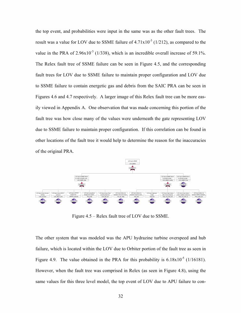
the top event, and probabilities were input in the same was as the other fault trees. The
result was a value for LOV due to SSME failure of 4.71x10⁻³ (1/212), as compared to the
value in the PRA of 2.96x10⁻³ (1/338), which is an incredible overall increase of 59.1%.
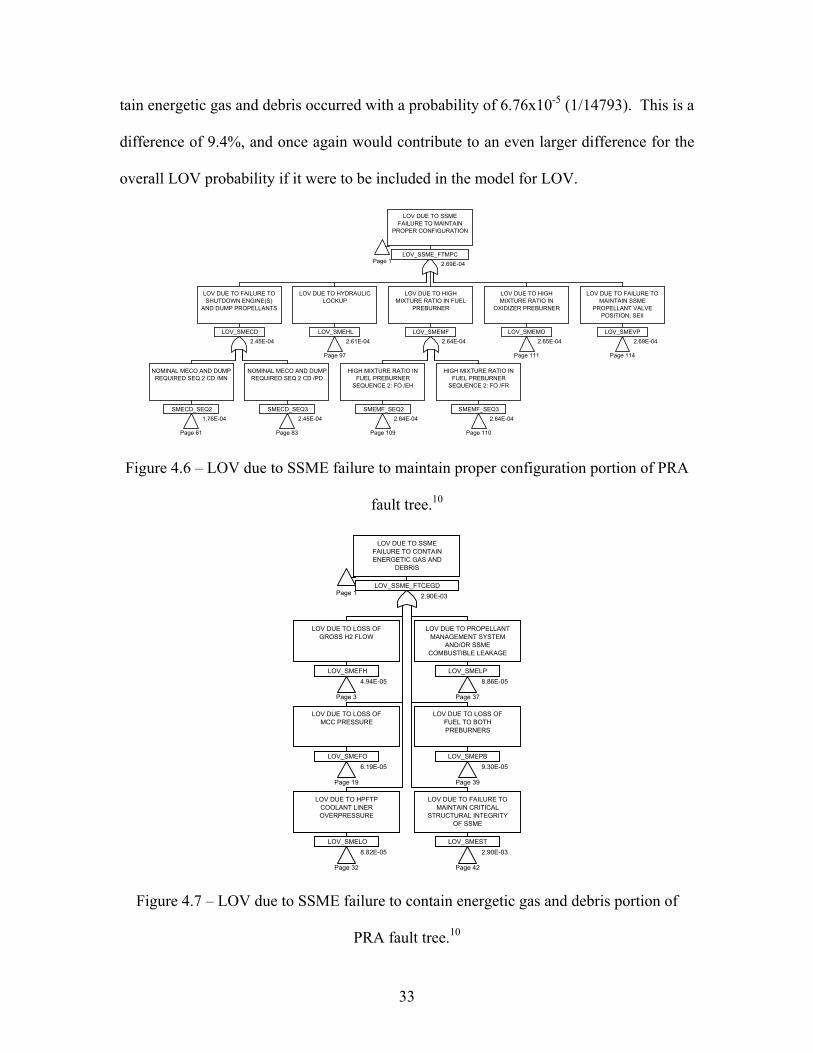
The Relex fault tree of SSME failure can be seen in Figure 4.5, and the corresponding
fault trees for LOV due to SSME failure to maintain proper configuration and LOV due
to SSME failure to contain energetic gas and debris from the SAIC PRA can be seen in
Figures 4.6 and 4.7 respectively. A larger image of this Relex fault tree can be more eas-
ily viewed in Appendix A. One observation that was made concerning this portion of the
fault tree was how close many of the values were underneath the gate representing LOV
due to SSME failure to maintain proper configuration. If this correlation can be found in
other locations of the fault tree it would help to determine the reason for the inaccuracies
of the original PRA.
LOV_SSME
LOV due to SSME
Q:0.0047111
LOV_SSME_Gas
LOV due to SSME failure to contain energetic gas ...
Q:0.0032811
Loss_H2_flow
LOV due to loss of gross H2 flow
Q:4.94e-005
Loss_MCC_pres
LOV due to loss of MCC pressure
Q:6.19e-005
HPFTP_overpres
LOV due to HPFTP coolant liner ...
Q:8.82e-005
Prop_leak
LOV due to propellant management system ...
Q:8.86e-005
Loss_fuel_pre
LOV due to loss of fuel to both preburners
Q:9.3e-005
Crit_str_integ
LOV due to failure to maintain critical structural ...
Q:0.0029
LOV_SSME_Config
LOV due to SSME failure to maintain proper ...
Q:0.001304
Fail_shut
LOV due to failure to shutdown engine(s) and ...
Q:0.000245
Hyd_lock
LOV due to hydraulic lockup
Q:0.000261
High_mix_ratio_fuel
LOV due to high mixture ratio in fuel preburner
Q:0.000264
High_mix_ratio_ox
LOV due to high mixture ratio in oxidizer preburner
Q:0.000265
Prop_valve_pos
LOV due to failure to maintain SSME propellant ...
Q:0.000269
LOV_SSME_Prop
LOV due to SSME failure to mainatain proper ...
Q:0.000126
The other system that was modeled was the APU hydrazine turbine overspeed and hub
failure, which is located within the LOV due to Orbiter portion of the fault tree as seen in
Figure 4.9. The value obtained in the PRA for this probability is 6.18x10⁻⁵ (1/16181).
However, when the fault tree was comprised in Relex (as seen in Figure 4.8), using the
same values for this three level model, the top event of LOV due to APU failure to con-
Figure 4.5 – Relex fault tree of LOV due to SSME.
33
tain energetic gas and debris occurred with a probability of 6.76x10⁻⁵ (1/14793). This is a
difference of 9.4%, and once again would contribute to an even larger difference for the
overall LOV probability if it were to be included in the model for LOV.
LOV DUE TO SSMEFAILURE TO MAINTAIN
PROPER CONFIGURATION
LOV_SSME_FTMPCPage 1 2.69E-04
LOV DUE TO FAILURE TOSHUTDOWN ENGINE(S)
AND DUMP PROPELLANTS
LOV_SMECD2.45E-04
NOMINAL MECO AND DUMPREQUIRED SEQ 2 CD /MN
SMECD_SEQ2
Page 61
1.76E-04
NOMINAL MECO AND DUMPREQUIRED SEQ 2 CD /PD
SMECD_SEQ3
Page 83
2.45E-04
LOV DUE TO HYDRAULICLOCKUP
LOV_SMEHL
Page 97
2.61E-04
LOV DUE TO HIGHMIXTURE RATIO IN FUEL
PREBURNER
LOV_SMEMF2.64E-04
HIGH MIXTURE RATIO INFUEL PREBURNER
SEQUENCE 2: FO /EH
SMEMF_SEQ2
Page 109
2.64E-04
HIGH MIXTURE RATIO INFUEL PREBURNER
SEQUENCE 2: FO /FR
SMEMF_SEQ3
Page 110
2.64E-04
LOV DUE TO HIGHMIXTURE RATIO IN
OXIDIZER PREBURNER
LOV_SMEMO
Page 111
2.65E-04
LOV DUE TO FAILURE TOMAINTAIN SSME
PROPELLANT VALVEPOSITION; SEII
LOV_SMEVP
Page 114
2.69E-04
Figure 4.6 – LOV due to SSME failure to maintain proper configuration portion of PRA
fault tree.10
LOV DUE TO SSMEFAILURE TO CONTAINENERGETIC GAS AND
DEBRIS
LOV_SSME_FTCEGDPage 1 2.90E-03
LOV DUE TO LOSS OFGROSS H2 FLOW
LOV_SMEFH
Page 3
4.94E-05
LOV DUE TO LOSS OFMCC PRESSURE
LOV_SMEFO
Page 19
6.19E-05
LOV DUE TO HPFTPCOOLANT LINEROVERPRESSURE
LOV_SMELO
Page 32
8.82E-05
LOV DUE TO PROPELLANTMANAGEMENT SYSTEM
AND/OR SSMECOMBUSTIBLE LEAKAGE
LOV_SMELP
Page 37
8.86E-05
LOV DUE TO LOSS OFFUEL TO BOTHPREBURNERS
LOV_SMEPB
Page 39
9.30E-05
LOV DUE TO FAILURE TOMAINTAIN CRITICAL
STRUCTURAL INTEGRITYOF SSME
LOV_SMEST
Page 42
2.90E-03
Figure 4.7 – LOV due to SSME failure to contain energetic gas and debris portion of
PRA fault tree.10

34
APU fail
LOV due to APU Failure
Q:6.7559e-005
2 APUs
2 APU units fail; Unsuccessful single ...
2 APUs - 1
APU turbine overspeed
Q:6.96e-005
2 APUs - 2
Turbine failure misses critical equipment; turbine ...
Q:0.108
2 APUs - 3
Second APU unit failed; APU turbine
Q:0.88
2 APUs - 4
Single APU unit RTL unsuccessful
Q:1
All APUs
All APU units fail; APU turbine overspeed/hub ...
All APUs - 1
APU turbine overspeed
Q:6.96e-005
All APUs - 2
Turbine failure misses critical equipment; turbine ...
Q:0.108
All APUs - 3
Second APU unit failed; APU turbine
Q:0.88
All APUs - 4
Third APU unit failed; APU turbine
Q:0.88
Critical Equipment
Flight critical equip fails; APU turbine ...
Critical Equipment - 1
APU turbine overspeed
Q:6.96e-005
Critical Equipment - 2
Hub breakup; APU turbine overspeed
Q:0.9
Critical Equipment - 3
Uncontained within APU; APU turbine
Q:1
Critical Equipment - 4
Flight critical equipment failure, APU
Q:0.88
Figure 4.8 – Relex FTA of LOV due to APU failure to contain energetic gas and debris.
LOV DUE TO APU/HYDTURBINE OVERSPEED/HUB
FAILURE
LOV_APUETUPage 364 5.65E-05
LOV 2 APU/HYD UNITSFAIL, UNSUCC SINGLE
LAND; TURBOVERSPEED/HUB FAILS;
ETU05LOV
Page 369
6.61E-07
LOV ALL APU/HYDUNITS FAIL; APU/HYD
TURBINE OVERSPEED/HUBFAILURE; SEQ. 6
ETU06LOV
Page 370
5.82E-06
FLIGHT CRITICALEQUIP FAILS; APU/HYD
TURBINE OVERSPEED/HUBFAILURE; SEQ. 7
ETU07LOV
Page 371
5.51E-05
LOV 2 APU/HYD UNITSFAIL, UNSUCC SINGLE
LAND; TURBOVERSPEED/HUB FAILS;
ETU05LOVPage 368 6.61E-07
APU/HYD TURBINEOVERSPEED
TU6.96E-05
TURBINE FAILUREMISSES CRITICALEQUIP; TURBINE
OVERSPEED/HUB
ETU05FCE1.08E-01
HUB BREAKUP; APU/HYDTURBINE OVERSPEED;
ENOAAHBA1IDTU059.00E-01
UNCONTAINED WITHINAPU; APU/HYD TURBINE
ENOAACOA1IDTU051.00E+00
FLIGHT CRITICALEQUIPMENT OK; APU/HYD
ENOAAOKA1OKTU051.20E-01
SECOND APU/HYD UNITFAILED; APU/HYD
TURBINE
ENOAASIA2IDTU058.80E-01
SINGLE APU/HYD UNITRTL UNSUCCESSFUL;
ENOAAFRA3ULTU051.00E-01
LOV ALL APU/HYDUNITS FAIL; APU/HYD
TURBINE OVERSPEED/HUBFAILURE; SEQ. 6
ETU06LOVPage 368 5.82E-06
APU/HYD TURBINEOVERSPEED
TU6.96E-05
TURBINE FAILUREMISSES CRITICALEQUIP; TURBINE
OVERSPEED/HUB
ETU06FCE1.08E-01
HUB BREAKUP; APU/HYDTURBINE OVERSPEED;
ENOAAHBA1IDTU069.00E-01
UNCONTAINED WITHINAPU; APU/HYD TURBINE
ENOAACOA1IDTU061.00E+00
FLIGHT CRITICALEQUIPMENT OK; APU/HYD
ENOAAOKA1OKTU061.20E-01
SECOND APU/HYD UNITFAILED; APU/HYD
TURBINE
ENOAASIA2IDTU068.80E-01
THIRD APU/HYD UNITFAILED; APU/HYD
TURBINE
ENOAASIA3IDTU068.80E-01
FLIGHT CRITICALEQUIP FAILS; APU/HYD
TURBINE OVERSPEED/HUBFAILURE; SEQ. 7
ETU07LOVPage 368 5.51E-05
APU/HYD TURBINEOVERSPEED
TU6.96E-05
HUB BREAKUP; APU/HYDTURBINE OVERSPEED;
ENOAAHBA1IDTU079.00E-01
UNCONTAINED WITHINAPU; APU/HYD TURBINE
ENOAACOA1IDTU071.00E+00
FLIGHT CRITICALEQUIPMENT FAILURE;
APU/HYD
ENOAACEA1IDTU078.80E-01
Figure 4.9 – All four parts of the PRA fault tree associated with APU hydrazine turbine
overspeed and hub failure.10
35
With all of the discrepancies encountered throughout this study, the most likely explana-
tion would be that the software used for the PRA (CAFTA) used approximations to de-
crease computation time. However, these compiling approximations, although typically
small and sometimes even insignificant for many cases, have proven here to be large
enough to make the model much less accurate than initially considered.
4.3 BlockSim RBD
The tool used to create and perform the RBD analyses of systems as well as the overall
LOV probability of the Space Shuttle is called BlockSim. BlockSim was first used to
create an RBD of the overall LOV, once again using the inputs from the PRA done by
SAIC. The same level of detail was used for each model, in order to ensure accuracy
when comparing the results of the different models, and the BlockSim RBD modeling
LOV can be seen in Figure 4.10. The result of the overall LOV was a failure probability
of 8.1x10⁻³, which is the same result gained by use of the Relex analysis. This is what
was expected, considering that both FTA and RBD are based on the same logic princi-
ples.
BlockSim was then used to model the failure of the SSME as a RBD. Since all of the
events within the SSME system fault tree that had been modeled were related through
“OR” gates, all of the events could simply connected in series in any order to form the
RBD. Therefore, all of the third level events (which is the same level of detail used in the
fault tree) were connected in series, at which point the probabilities were taken from the

36
PRA and the analysis was completed. This RBD is shown in Figure 4.11. The result was
a probability of failure of 4.7x10⁻³, which is once again identical to the probability gained
through FTA.
Figure 4.10 – BlockSim RBD of three-level LOV.
Figure 4.11 – BlockSim RBD of LOV due to SSME.
In order to create a RBD to model APU hydrazine turbine overspeed and hub failure, it
involved more than just putting all of the events in series. Since there are three “AND”
gates in the FTA (for this level of detail) of this system, the model was created as a series
of three sets of four parallel events, because in each case all four events would need to
occur to have that particular failure. The RBD representing this model is illustrated in
Figure 4.12. The probability of APU hydrazine turbine overspeed and hub failure at-

37
tained from this RBD is 6.76x10⁻⁵, which is once again identical to the results of the as-
sociated fault tree as was expected.
Figure 4.12 – BlockSim RBD of APU hydrazine turbine overspeed and hub failure.
Table 4.1 – Comparison of Reliability Analysis Techniques.
Model (Lev-els of Detail)
Top Event Probability
(Relex)
Top Event Failure Rate
(Relex)
Top Event Probability (BlockSim)
Top Event Failure Rate (BlockSim)
Top Event Probability
(PRA)
Top Event Failure
Rate (PRA)
Relative In-crease as com-pared to PRA
LOV (2) 7.80E-03 1/128 7.80E-03 1/128 7.66E-03 1/131 1.8%
LOV (3) 8.09E-03 1/124 8.09E-03 1/124 7.66E-03 1/131 5.6%
LOV (4) 9.11E-03 1/110 9.11E-03 1/110 7.66E-03 1/131 18.9%
LOV due to SSME (3) 4.71E-03 1/212 4.71E-03 1/212 2.96E-03 1/338 59.1%
APU hydra-zine turbine overspeed and hub failure (3)
6.76E-05 1/14792 6.76E-05 1/14792 6.18E-05 1/16181 9.4%

38
5. Conclusions
The most popular technique being used today for quantitative reliability analysis in aero-
space engineering is by far FTA. However, it has been argued by many that RBD is a
better technique, while just as accurate as FTA. One of the largest points in this argu-
ment is that FTA and RBD are based on the same principles of probability, but that RBD
is capable of modeling more complicated situations. For instance, an example often used
is the “bridge gate” in RBD, which cannot be simply modeled in FTA without some sort
of repetitive model representing all of the minimum cut sets. Figure 5.1 shows a simple
RBD with a bridge structure, and Figure 5.2 shows the fault tree that would represent the
same model. With that in mind, if the same system is modeled in both FTA and RBD,
the results of the analysis should be identical in both methods. This phenomenon can be
seen by comparing the results of the models completed in both Relex and BlockSim.
Therefore if the comparison were merely based on accuracy of the models, both methods
would be seen as the same.
A
E
C D
BA
E
C D
B
Figure 5.1 – Bridge structure RBD.

39
Unfortunately there was not sufficient means to create large models in order to compare
the analysis times required for each. In addition, those might vary according to the tool
used in order to perform each analysis, and would not be specific to each analysis tech-
nique. Since the results of the same system being modeled in these two methods do not
vary, the process of compiling the models and working with them prior to analysis must
be considered for comparison.
Top Event
A D E A C B D CB E
Top Event
A D E A C B D CB E
Figure 5.2 – Necessary FTA of a bridge structure.
One consideration was how convenient and easy the models would be to create. It was
originally hypothesized that the RBD model would be the simplest model to create, since
in most cases (especially in modeling the Space Shuttle which has very little redundancy
at these high levels) the events would just have to be put in series and defined just as they
are in FTA. The surprising conclusion here is that it is the simplicity of this model that
makes it somewhat difficult to work with. One of the benefits of the fault tree that was

40
not previously considered is the inherent organization that comes with the creation of a
fault tree. The process of creating such a top-down approach model helps to organize all
of the events much more than if the same model is created in a bottom-up approach such
as RBD. It becomes much easier to find a specific event in a model, or trace the effects
of a given event when the model has been broken down from a system level all the way
to the component level (and sometimes even to more detail). However, when the out-
come of a model is obtained merely by listing every basic event it is very hard to follow
and stay aware of which events have already been added when first creating the model.
Another benefit of FTA is that when analyzing a complicated model, one can obtain the
probabilities associated with failure of a subsystem within that model without creating an
entirely new model for it. If a complex system is being considered, the failure probability
of any subsystem within the model must be calculated in order to then be used in calcula-
tion of the failure probability of the next level up from that. However, in RBD the sub-
systems are not necessarily identified, and since it is merely the accumulation of all of the
basic events, in order to get the failure probability of a subsystem, one would need to cre-
ate a new model to obtain this value. The only down side to this is that FTA must per-
form more calculations in order to get the system failure probability, and in a very large
and complex model such as the one compiled to analyze the Space Shuttle, this can be a
significant amount of analysis time. But since analysis techniques, as well as computer
technology have come a long way in the last several years, this has become a less impor-
tant factor to consider when deciding on which analysis technique to use.

41
The time it took to set up and execute the different models was also initially hypothesized
to be a factor in which technique was better overall. However, through the completion
of this work that factor has not come into play. The time to set up the same model in ei-
ther a FTA software package or a RBD software package (assuming the user is an experi-
enced one) is very similar. For the models created in this study, the time to set one up
should be on the order of several hours to a day for an experienced user. This is the same
for both software packages used. And due to the constant improvement of computation
time of both software packages and computers in general, computation time for these
models was on the order of seconds. Given, models of the size of the PRA would take
significantly longer to compile and compute, but computation time should not be any dif-
ferent for the two techniques here, and the time to set up the same model in each should
be comparable.
In summary, there are of course advantages and disadvantages to all methods being con-
sidered. There is no one analysis technique that is superior to all others for every case,
and decisions on which technique is to be used to analyze a given system should always
be made on a case by case basis. However, when it comes to a system that will not nec-
essarily be modeled most accurately by a specific method, sometimes it is the user’s
needs and preferences that are responsible for this choice. Depending on the application
of the results that are to be obtained, this may be the best way to choose an analysis
method in some cases since the majority of the time involved in an analysis is the time
associated with the compilation of the model.

42
Appendix A – Relex Fault Trees
LOV STS
Loss of Space Transportation System ...
Q:0.00808723
LOV SSME
LOV due to SSME
Q:0.00329382
LOV SSME 1
LOV due to SSME failure to contain gas and ...
Q:0.0029
LOV SSME 2
LOV due to SSME failure to maintain proper ...
Q:0.000126
LOV SSME 3
LOV due to SSME failure to maintain proper ...
Q:0.000269
LOV ET
LOV due to External Tank failure
Q:0.000192
LOV Landing
LOV due to landing failure or error
Q:0.000411
SRB
LOV due to Solid Rocket Boosters
Q:0.00126
Orbiter
LOV due to Orbiter
Q:0.00295259
LOV Orbiter 1
LOV due to Orbiter failure to contain gas and ...
Q:6.48e-005
LOV Orbiter 2
LOV due to Orbiter failure to maintain proper ...
Q:0.0017
LOV Orbiter 3
LOV due to Orbiter failure to maintain thermal ...
Q:0.00119
Relex fault tree of LOV with three levels of detail.

43
LOV STS
Loss of Space Transportation System ...
Q:0.00911346
LOV SSME
LOV due to SSME
Q:0.00432501
LOV SSME 1
LOV due to SSME failure to contain gas and ...
Q:0.0029
LOV SSME 2
LOV due to SSME failure to maintain proper ...
Q:0.000126
LOV SSME 3
LOV due to SSME failure to maintain proper ...
Q:0.00130332
LOV SSME 3.1
LOV due to failure to shutdown engine(s) and ...
Q:0.000245
LOV SSME 3.2
LOV due to hydraulic lockup
Q:0.000261
LOV SSME 3.3
LOV due to high mixture ratio in fuel preburner
Q:0.000264
LOV SSME 3.4
LOV due to high mixture ratio in oxidizer preburner
Q:0.000265
LOV SSME 3.5
LOV due to failure to maintain SSME propellant ...
Q:0.000269
LOV ET
LOV due to External Tank failure
Q:0.000192
LOV Landing
LOV due to landing failure or error
Q:0.000411
SRB
LOV due to Solid Rocket Boosters
Q:0.00126
Orbiter
LOV due to Orbiter
Q:0.00295259
LOV Orbiter 1
LOV due to Orbiter failure to contain gas and ...
Q:6.48e-005
LOV Orbiter 2
LOV due to Orbiter failure to maintain proper ...
Q:0.0017
LOV Orbiter 3
LOV due to Orbiter failure to maintain thermal ...
Q:0.00119
Relex fault tree of LOV with three levels of detail, and additional detail under LOV due to SSME failure to maintain
proper configuration.

44
LOV_SSME
LOV due to SSME
Q:0.0047111
LOV_SSME_Gas
LOV due to SSME failure to contain energetic gas ...
Q:0.0032811
Loss_H2_flow
LOV due to loss of gross H2 flow
Q:4.94e-005
Loss_MCC_pres
LOV due to loss of MCC pressure
Q:6.19e-005
HPFTP_overpres
LOV due to HPFTP coolant liner ...
Q:8.82e-005
Prop_leak
LOV due to propellant management system ...
Q:8.86e-005
Loss_fuel_pre
LOV due to loss of fuel to both preburners
Q:9.3e-005
Crit_str_integ
LOV due to failure to maintain critical structural ...
Q:0.0029
LOV_SSME_Config
LOV due to SSME failure to maintain proper ...
Q:0.001304
Fail_shut
LOV due to failure to shutdown engine(s) and ...
Q:0.000245
Hyd_lock
LOV due to hydraulic lockup
Q:0.000261
High_mix_ratio_fuel
LOV due to high mixture ratio in fuel preburner
Q:0.000264
High_mix_ratio_ox
LOV due to high mixture ratio in oxidizer preburner
Q:0.000265
Prop_valve_pos
LOV due to failure to maintain SSME propellant ...
Q:0.000269
LOV_SSME_Prop
LOV due to SSME failure to mainatain proper ...
Q:0.000126
Relex fault tree of LOV due to SSME with three levels of detail.
APU fail
LOV due to APU Failure
Q:6.7559e-005
2 APUs
2 APU units fail; Unsuccessful single ...
Q:6.61478e-006
2 APUs - 1
APU turbine overspeed
Q:6.96e-005
2 APUs - 2
Turbine failure misses critical equipment; turbine ...
Q:0.108
2 APUs - 3
Second APU unit failed; APU turbine
Q:0.88
2 APUs - 4
Single APU unit RTL unsuccessful
Q:1
All APUs
All APU units fail; APU turbine overspeed/hub ...
Q:5.82101e-006
All APUs - 1
APU turbine overspeed
Q:6.96e-005
All APUs - 2
Turbine failure misses critical equipment; turbine ...
Q:0.108
All APUs - 3
Second APU unit failed; APU turbine
Q:0.88
All APUs - 4
Third APU unit failed; APU turbine
Q:0.88
Critical Equipment
Flight critical equip fails; APU turbine ...
Q:5.51232e-005
Critical Equipment - 1
APU turbine overspeed
Q:6.96e-005
Critical Equipment - 2
Hub breakup; APU turbine overspeed
Q:0.9
Critical Equipment - 3
Uncontained within APU; APU turbine
Q:1
Critical Equipment - 4
Flight critical equipment failure, APU
Q:0.88
Relex fault tree of APU hydrazine turbine overspeed and hub failure with three levels of detail.

45
REFERENCES 1 Blischke, Wallace R., & Murthy, D. N. Prabhakar. Reliability: Modeling, Prediction
and Optimization. John Wiley & Sons, Inc. New York, NY. 2000. 2 The Flight of STS-1. (http://history.nasa.gov/sts1/) 3 Columbia Accident Investigation Board: Report Volume I. August 26, 2003.
(http://boss.streamos.com/download/caib/report/web/full/caib_report_volume1.pdf) 4 Jenkins, Dennis R. Space Shuttle: The History of the National Space Transportation
System, The First 100 Missions. Cape Canaveral, Florida. 2002. 5 Heppenheimer, T. A. Development of the Space Shuttle, 1972-1981 (History of the
Space Shuttle Volume 2). Smithsonian Institution Press. Washington, D. C. April 2002.
6 Report of the Presidential Commission on the Space Shuttle Challenger Accident.
June 6, 1986. (http://science.ksc.nasa.gov/shuttle/missions/51-l/docs/rogers-commission/table-of-contents.html)
7 System Analysis Reference: Reliability, Availability and Optimization. ReliaSoft Pub-
lishing. Tuscon, AZ. 1999. (http://www.weibull.com/systemrelwebcontents.html) 8 Pukite, Jan, & Pukite, Paul. Modeling for Reliability Analysis: Markov Modeling for
Reliability, Maintainability, Safety, and Supportability Analyses of Complex Sys-tems. Wiley-IEEE Computer Society Press. New York, NY. 2001.
9 O’Connor, Patrick D. T. Practical Reliability Engineering. John Wiley & Sons, Ltd.
Chichester, England. 2002. 10 Fragola, J. R. “Space Shuttle Probabilistic Risk Assessment”. Proceedings of
PSAMIII, Crete, Greece. 1996