Reliability Analysis of Flood Sea Defence Structures … · Integrated Flood Risk Analysis and...
121
Integrated Flood Risk Analysis and Management Methodologies Reliability Analysis of Flood Sea Defence Structures and Systems MAIN TEXT Date April 2008 Report Number T07-08-01 Revision Number 1_2_P01 Deliverable Number: D7.1 Due date for deliverable: February 2008 Actual submission date: April 2008 Task Leader 12 FLOODsite is co-funded by the European Community Sixth Framework Programme for European Research and Technological Development (2002-2006) FLOODsite is an Integrated Project in the Global Change and Eco-systems Sub-Priority Start date March 2004, duration 5 Years Document Dissemination Level PU Public PU PP Restricted to other programme participants (including the Commission Services) RE Restricted to a group specified by the consortium (including the Commission Services) CO Confidential, only for members of the consortium (including the Commission Services) Co-ordinator: HR Wallingford, UK Project Contract No: GOCE-CT-2004-505420 Project website: www.floodsite.net
-
Upload
truongdang -
Category
Documents
-
view
219 -
download
1
Transcript of Reliability Analysis of Flood Sea Defence Structures … · Integrated Flood Risk Analysis and...

Integrated Flood Risk Analysis and Management Methodologies
Reliability Analysis of Flood Sea Defence Structures and Systems MAIN TEXT
Date April 2008
Report Number T07-08-01 Revision Number 1_2_P01
Deliverable Number: D7.1 Due date for deliverable: February 2008 Actual submission date: April 2008 Task Leader 12
FLOODsite is co-funded by the European Community Sixth Framework Programme for European Research and Technological Development (2002-2006)
FLOODsite is an Integrated Project in the Global Change and Eco-systems Sub-Priority Start date March 2004, duration 5 Years
Document Dissemination Level
PU Public PU PP Restricted to other programme participants (including the Commission Services) RE Restricted to a group specified by the consortium (including the Commission Services) CO Confidential, only for members of the consortium (including the Commission Services)
Co-ordinator: HR Wallingford, UK
Project Contract No: GOCE-CT-2004-505420
Project website: www.floodsite.net

T07_08_01_Reliability_Analysis_D7_1 10 April 2008
DOCUMENT INFORMATION
Title Reliability Analysis of Flood Sea Defence Structures and Systems Main Text
Lead Author Pieter van Gelder
Contributors
TUD Foekje Buijs, Cong Mai Van, Wouter ter Horst, Wim Kanning, Mohammad Nejad, Sayan Gupta, Reza Shams, Noel van Erp HRW Ben Gouldby, Greer Kingston, Paul Sayers, Martin Wills LWI Andreas Kortenhaus, Hans-Jörg Lambrecht
Distribution Public Document Reference T 0 7 -08-01 Appendix
DOCUMENT HISTORY
Date Revision Prepared by Organisation Approved by Notes 01/01/08 1.1.p12 P. van Gelder TUD 01/04/08 1.1.p12 C. Mai Van TUD 09//04/08 1.1p12 P. van Gelder TUD Corrupted Word version
replaced 10/04/08 1.2P01 Paul Samuels HR Wallingford Formatted as a deliverable
ACKNOWLEDGEMENT The work described in this publication was supported by the European Community’s Sixth Framework Programme through the grant to the budget of the Integrated Project FLOODsite, Contract GOCE-CT-2004-505420. DISCLAIMER This document reflects only the authors’ views and not those of the European Community. This work may rely on data from sources external to the FLOODsite project Consortium. Members of the Consortium do not accept liability for loss or damage suffered by any third party as a result of errors or inaccuracies in such data. The information in this document is provided “as is” and no guarantee or warranty is given that the information is fit for any particular purpose. The user thereof uses the information at its sole risk and neither the European Community nor any member of the FLOODsite Consortium is liable for any use that may be made of the information. © FLOODsite Consortium

Task 7 Reliability Analysis D7.1 Contract No:GOCE-CT-2004-505420
T07_08_01_Reliability_Analysis_D7_1 i 10 April 2008
SUMMARY Risk identification consists of defining the hazard, loss causing event E, probability P(E) of that event, perception Pe(E,P(E)) and consequences C(Pe) of that perception. Risk identification is followed by risk management, whose purpose is to mitigate the risks, for example by reducing P(E) or C(Pe) and providing suitable risk communication to the population at risk. Task 7 has focused in this approach for the safety issues of flood defences on the failure probability P(E). It has been subdivided into 4 activities, which are: - preliminary probability analyses of flood defences - uncertainty analyses of all issues which are related to flood defences - review and development of software codes for reliability calculation - applicability of improved methods
The defence reliability analysis has been developed in this task to support a range of decisions and adopt different levels of complexity (feasibility, preliminary and detailed design). Each tier in the analysis of the reliability of the defence and defence system demands different levels of data on the condition and form of the defence and its exposure to load, but also different types of models from simple to complex. As a result each level will be capable of resolving increasing complex limit state functions. During the project, these levels has been considered and complexity of models and amount of data has been adjusted accordingly.
At the beginning of any flood risk project a very limited physical knowledge will be available on failure modes, their interactions, and the associated prediction models, including the uncertainties of the input data and models. The 1st activity of Task 7 has shown how to deal with such situation. For this purpose, three selected pilot sites in different countries and from different areas (coast, estuary, river) have been used. The main outputs and benefits from this activity were (i) the relative importance of the uncertainties and their possible contributions to the probability of flooding, (ii) the gaps related to prediction models and limit state equations by means of a detailed top-down analysis; (iii) the uncertainties which are worth reducing by the generation of new knowledge, (iv) the priorities with respect to the allocation of research efforts for the various topics to be addressed in the other sub-projects, (v) the areas of high, low and medium uncertainty.
Task 7 has investigated how to specify uncertainties for models and parameters to be used in FLOODsite. Special care has been taken to make the report compatible with the LOR (language of risk) document. The work has been focused on scoping and reviewing possible approaches for uncertainty database formats in order to develop an uncertainty categorisation system. Default distribution types and parameters to all load – and resistance variables are included in the system.

Task 7 Reliability Analysis D7.1 Contract No:GOCE-CT-2004-505420
T07_08_01_Reliability_Analysis_D7_1 ii 10 April 2008
Task 7 furthermore focused on the development of fault trees of different flood defence types and used as input the results of the Task 4 failure mode report. The fault trees contain components which consist of complex numerical models such as geotechnical FEM. Furthermore calculation routines for a software tool have been programmed which take into account differences between explicit limit state equations and implicit numerical models. A user interface has been developed in order to run the calculation routines as user friendly as possible.
The reliability tool is applied to the German Bight Coast case study site and compared to the results obtained with the preliminary reliability analysis. The German Bight Coast flood defence system is a complex system. The alignment of the system consists of a varying foreland, a major dike line and a second dike line. Failures in the past have not been reported though considerable overtopping has been observed at a number of locations. The probabilities of failure calculated with the new reliability tool are higher than the results obtained with the preliminary reliability analysis, although the comparison was not the main goal of this study. The difference is explained firstly by the different arrangement of the fault tree of the reliability tool as compared to the scenario tree applied in the German Bight Coast case study. A second explanation is a difference in limit state equations applied in the reliability tool as compared to the preliminary reliability analysis of the German Bight Coast, e.g. erosion or overtopping equations. A third explanation for the higher probability of failure is the application of different distribution functions and associated parameters. Comparisons between different reliability calculation methods are difficult to make because of the large number of changing parameters. The newly developed reliability tool however has shown its applicability to practice.

Task 7 Reliability Analysis D7.1 Contract No:GOCE-CT-2004-505420
T07_08_01_Reliability_Analysis_D7_1 iii 10 April 2008
CONTENTS Document Information .............................................................................................................................................. Document History ..................................................................................................................................................... Acknowledgement ..................................................................................................................................................... Disclaimer............................................................................................................................................................... 2 Summary .................................................................................................................................................................. i Contents ................................................................................................................................................................. iii
1 INTRODUCTION........................................................................................................................................ 7
1.1 BACKGROUND ........................................................................................................................................ 7 1.2 PURPOSE AND OBJECTIVES ..................................................................................................................... 7 1.3 PROBLEM DEFINITION............................................................................................................................. 7 1.4 APPROACH ............................................................................................................................................. 8 1.5 ACTIVITIES ............................................................................................................................................. 9 1.6 RELATIONSHIP TO OVERALL PROJECT OBJECTIVES ................................................................................. 9 1.7 DISSEMINATION AND COMMUNICATION ACTIVITIES ............................................................................. 11
2 RELIABILITY ANALYSIS OF FLOOD DEFENCE SYSTEMS ......................................................... 14
2.1 INTRODUCTION..................................................................................................................................... 14 2.2 PROBABILISTIC VERSUS DETERMINISTIC APPROACH OF THE DESIGN..................................................... 17 2.3 UNCERTAINTIES ................................................................................................................................... 18
2.3.1 Inherent uncertainty in time ............................................................................................................ 19 2.3.2 Inherent uncertainty in space.......................................................................................................... 20 2.3.3 Parameter uncertainty..................................................................................................................... 21 2.3.4 Distribution type uncertainty .......................................................................................................... 22 2.3.5 Model uncertainty ........................................................................................................................... 23 2.3.6 Uncertainties related to the construction........................................................................................ 24 2.3.7 Reduction of uncertainty ................................................................................................................. 26
2.4 PROBABILISTIC APPROACH OF THE DESIGN .......................................................................................... 26 2.4.1 System analysis................................................................................................................................ 27 2.4.2 Simple systems................................................................................................................................. 28 2.4.3 Example: Risk analysis of a polder ............................................................................................... 30 2.4.4 Failure probability of a system ...................................................................................................... 32 2.4.5 Estimation of the probability of a failure mode of an element ........................................................ 35
3 PRELIMINARY RELIABILITY ANALYSIS ........................................................................................ 41
3.1 PRA FOR TEST PILOT SITE THAMES ...................................................................................................... 41 3.2 PRA FOR TEST PILOT SITE SCHELDT ..................................................................................................... 44 3.3 PRA FOR TEST PILOT SITE GERMAN BIGHT .......................................................................................... 49
4 UNCERTAINTY ANALYSIS ................................................................................................................... 54
4.1 INTRODUCTION..................................................................................................................................... 54 4.2 TYPES OF UNCERTAINTY....................................................................................................................... 54
4.2.1 Uncertainties ................................................................................................................................... 54 4.2.2 Definitions....................................................................................................................................... 54 4.2.3 Natural variability........................................................................................................................... 56 4.2.4 Knowledge uncertainties ................................................................................................................. 58 4.2.5 Correlations between uncertainties................................................................................................. 61
4.3 CLASSIFICATION OF UNCERTAINTIES .................................................................................................... 64 4.3.1 General overview ............................................................................................................................ 64 4.3.2 Probability of failure of a dike ........................................................................................................ 64 4.3.3 Failure mechanisms ........................................................................................................................ 65 4.3.4 Classification .................................................................................................................................. 65

Task 7 Reliability Analysis D7.1 Contract No:GOCE-CT-2004-505420
T07_08_01_Reliability_Analysis_D7_1 iv 10 April 2008
4.4 RANKING OF UNCERTAINTIES ............................................................................................................... 71 4.4.1 Case studies..................................................................................................................................... 71 4.4.2 Sensitivity coefficients case studies ................................................................................................. 73 4.4.3 Ranking of uncertainties.................................................................................................................. 75
4.5 DEALING WITH UNCERTAINTIES ........................................................................................................... 76 4.5.1 Effects of uncertainties .................................................................................................................... 76 4.5.2 Reduction of uncertainty ................................................................................................................. 76 4.5.3 Remaining uncertainties of the reliability index.............................................................................. 77 4.5.4 How to deal with uncertainties........................................................................................................ 78
4.6 CONCLUSIONS ...................................................................................................................................... 81 4.7 DATABASE OF UNCERTAINTIES FOR MODELS AND PARAMETERS .......................................................... 81
5 FAULT TREE GENERATION ................................................................................................................ 82
5.1 REMARKS ON THE CONSTRUCTION OF FAULT TREES AND FAULT TREE ANALYSIS (FTA)..................... 82 5.1.1 Introduction..................................................................................................................................... 82 5.1.2 Construction of a fault tree ............................................................................................................. 82 5.1.3 Difficulties and problems concerning fault trees for flood defences ............................................... 83
5.2 ELABORATION OF FAULT TREE FOR A MASS (CONCRETE) VERTICAL OR BATTERED WALL..................... 86 5.2.1 Reference table and entry codes...................................................................................................... 86 5.2.2 Graphical representations of failure modes.................................................................................... 89 5.2.3 Fault tree of a mass (concrete) vertical or battered wall................................................................ 93
6 DEVELOPMENT OF SOFTWARE RELIABILITY TOOL AND APPLICABILITY ...................... 93
6.1 INTRODUCTION..................................................................................................................................... 93 6.2 OVERVIEW OF RELIABILITY SOFTWARE ................................................................................................ 93
6.2.1 Basics .............................................................................................................................................. 93 6.2.2 System requirements........................................................................................................................ 93
6.3 DESCRIPTION OF THE SYSTEM COMPONENTS ........................................................................................ 93 6.3.1 Limit state equations ....................................................................................................................... 93 6.3.2 LSE parameters and uncertainties .................................................................................................. 93 6.3.3 Fault Trees ...................................................................................................................................... 93 6.3.4 Interface .......................................................................................................................................... 93
6.4 EXAMPLE USE OF THE TOOL.................................................................................................................. 93 6.4.1 Overview ......................................................................................................................................... 93 6.4.2 Fault tree construction.................................................................................................................... 93 6.4.3 Distribution selection ...................................................................................................................... 93 6.4.4 Results ............................................................................................................................................. 93
6.5 OTHER FLOOD DEFENCE RELIABILITY SOFTWARE AND THE FLOODSITE RELIABILITY TOOL.................. 93 6.6 AREAS FOR IMPROVEMENT OF FLOODSITE RELIABILITY TOOL.............................................................. 93
7 IDENTIFICATION OF KEY AREAS FOR FURTHER RESEARCH ................................................ 93
7.1 KEY AREAS FOR FURTHER RESEARCH ................................................................................................... 93 7.2 COMPLEX FAILURE MODELS ................................................................................................................. 93 7.3 TIME DEPENDENT PROCESSES ............................................................................................................... 93 7.4 SENSITIVITY ANALYSIS......................................................................................................................... 93
LIST OF REFERENCES ................................................................................................................................... 93 APPENDIX 1: DETAILS OF THE PRA THAMES........................................................................................ 93 APPENDIX 2: DETAILS OF THE PRA SCHELDT ...................................................................................... 93 APPENDIX 3: DETAILS OF THE PRA GERMAN BIGHT ......................................................................... 93 APPENDIX 4: UNCERTAINTY DATABASE ................................................................................................ 93 APPENDIX 5: USER MANUAL RELIABILITY TOOL ............................................................................... 93 LIST OF FIGURES
Figure 1.1 Methodology of Theme 1________________________________________________________ 10 Figure 1.2 Structure of Sub-Theme 1.2______________________________________________________ 10 Figure 2.1 Different safety level for the same design____________________________________________ 17 Figure 2.2 Sections of a dike ______________________________________________________________ 18

Task 7 Reliability Analysis D7.1 Contract No:GOCE-CT-2004-505420
T07_08_01_Reliability_Analysis_D7_1 v 10 April 2008
Figure 2.3 Probabilistic approach of the design _______________________________________________ 27 Figure 2.4 Input-Output model ____________________________________________________________ 28 Figure 2.5 Fault tree ____________________________________________________________________ 28 Figure 2.6 Parallel and series system _______________________________________________________ 28 Figure 2.7 A chain as a series system _______________________________________________________ 29 Figure 2.8 A frame as a parallel system _____________________________________________________ 29 Figure 2.9 Fault tree of a parallel system _____________________________________________________ 29 Figure 2.10 Fault tree of a series system _____________________________________________________ 29 Figure 2.11 Elements of a parallel system as series systems of failure modes _________________________ 30 Figure 2.12 Flood defence system and its elements presented in a fault tree _________________________ 31 Figure 2.13 Failure modes of a dike (Vrijling, 1986) ___________________________________________ 31 Figure 2.14 A dike section as a series system of failure modes ___________________________________ 32 Figure 2.15 The sluice as a series system of failure modes _______________________________________ 32 Figure 2.16 Fault trees for parallel and series system __________________________________________ 33 Figure 2.17 Combined events _____________________________________________________________ 33 Figure 2.18 Probability of A or B given ρ ___________________________________________________ 34 Figure 2.19 probability of failure of a series system ____________________________________________ 35 Figure 2.20 Reliability function ____________________________________________________________ 36 Figure 2.21 Probability distribution and probability density _____________________________________ 36 Figure 2.22 Components of the failure probability _____________________________________________ 37 Figure 2.23 Joint probability density function_________________________________________________ 37 Figure 2.24 Probability density of the Z-function ______________________________________________ 39 Figure 2.25 Adapted normal distribution ____________________________________________________ 40 Figure 3.1 Location of Dartford Creek, Gravesend and the Thames barrier at Greenwich in the Thames Estuary______________________________________________________________________________________ 41
Figure 3.2 The Flood defence structure types, their primary function, site specific failure processes and the failure mechanisms which were included in the reliability analysis. _________________________________ 42 Figure 3.3: Fragility for earth embankment section 4. The failure mechanism driven by a combination of uplifting and piping dominates the total fragility curve.___________________________________________ 43 Figure 3.4: Fragility curves for three different types of reinforced concrete walls ______________________ 43 Figure 3.5: Source-Pathway-Receptor Model applied to the pilot site “German Bight Coast” Error! Bookmark not defined. Figure 3.6: Map of pilot site ‘German Bight’ (red line illustrates the coastal dike) _____________________ 50 Figure 3.7: Height of costal defence structures at pilot site ‘German Bight’___________________________ 51 Figure 3.8: Typical fault tree for a dike section at “German Bight Coast” ____________________________ 52 Figure 4.1: Classification of uncertainties, after Van Gelder (2000) _________________________________ 56 Figure 4.2: Borges-Castanheta model for the combination of river and sea induced water levels (Vrouwenvelder, 2006) __________________________________________________________________________________ 62 Figure 4.3: Failure tree of a flood defences (Lassing et al, 2003) ___________________________________ 65 Figure 4.4: Considered dike rings in the case studies ____________________________________________ 71 Figure 4.5: Dike ring 7: Noordoostpolder _____________________________________________________ 72 Figure 4.6: Dike-ring 32: Zeeuws Vlaanderen __________________________________________________ 72 Figure 4.7: Dike ring 36: Land van Heusden / De Maaskant_______________________________________ 72 Figure 4.8: Influence uncertainty reduction on distribution reliability index after Slijkhuis et. al. (1999) ____ 77 Figure 4.9: Translation and rotation of the frequency curves as σB increases from 5%, 11% to 17%________ 80 Figure 5.1: Bow-tie principle _______________________________________________________________ 82

Task 7 Reliability Analysis D7.1 Contract No:GOCE-CT-2004-505420
T07_08_01_Reliability_Analysis_D7_1 vi 10 April 2008
Figure 5.2: Fault-tree with different layers ____________________________________________________ 85 Figure 6.1: Components of the Reliability calculator software _____________________________________ 93 Figure 6.2: Example fault tree for sheet pile wall analysis ________________________________________ 93 Figure 6.3: Reliability calculator interface ____________________________________________________ 93 Figure 6.4: Height of coastal defence structures at pilot site German Bight Coast (after MLR, 2001) ______ 93 Figure 6.5 Indication of relevant failure mechanisms in German Bight Coast case study_________________ 93 Figure 6.6 Scenario fault tree of a sea dike after Kortenhaus (2003)_________________________________ 93 Figure 6.7 Screenshot of reliability tool for the calculation of the probability of failure of section 2 of the German Bight flood defences._______________________________________________________________ 93 Figure 7.1: Flow chart for the calculation of the probability of failure in a period of time (right) and the calculation of fragility (left). ________________________________________________________________ 93
LIST OF TABLES
Table 4.1: Used terms to describe two types of uncertainty (based on Christian, 2004, Baecher & Christian,2003 and National Research Council,1995) ________________________________________________________ 55 Table 4.2: General classification uncertainties based on Van der Most and Wehrung (2005) _____________ 64 Table 4.3: Classification of uncertainties ______________________________________________________ 65 Table 4.4: Dominant failure mechanisms of the considered dike rings _______________________________ 73 Table 4.5: Highest sensitivity coefficient dike ring 7: Noordoostpolder_______________________________ 73 Table 4.6: Highest sensitivity coefficients dike ring 36: Land van Heusden / De Maaskant _______________ 74 Table 4.7: Multiplication factors ____________________________________________________________ 79 Table 5.1: Failure modes (entries) present in fault tree ___________________________________________ 86 Table 6.1: Overview of the results of the probabilistic calculations for all sections in the preliminary reliability analysis of the German Bight flood defences (from Floodsite, 2006)_________________________________ 93 Table 6.2: Overview of the overall probability of failure for each flood defence section in the preliminary reliability analysis (from Floodsite, 2006) _____________________________________________________ 93 Table 6.3: Overview of the possibilities of different types of flood defence reliability software. ____________ 93 Table 6.4: Overview of suggestions for improvement of Floodsite reliability tool _______________________ 93

Task 7 Reliability Analysis D7.1 Contract No:GOCE-CT-2004-505420
T07_08_01_Reliability_Analysis_D7_1 7 1 April 2008
1 Introduction
1.1 Background
The context of the research is in the field of structural reliability of flood defences. A list of important literature is added at the end of this final report. The main previous projects which contributed knowledge to this area and related research in progress were:
PROVERBS (Probabilistic design tools for vertical breakwaters), completed in 1999, contract no. MAS3-CT95-0041, has developed and implemented probability based methods for the design of monolithic coastal structures and breakwaters subject to sea wave attack.
PRODEICH (Probabilistic design guidelines for seadikes), completed in 2002, funded by the German BMBF (Ministry for Education and Research in Germany) has concentrated on assessing the overall failure probabilities for a range of seadikes in Germany. Within this project all failure modes of seadikes have been extensively reviewed and limit state equations have been derived, including uncertainties.
Furthermore, a number of national projects undertaken in the UK by HRW for the Environment Agency has supported this task. These include the on-going project RASP-Risk Assessment for Strategic Planning that is currently developing a hierarchy of risk assessment methodologies to support national, regional and local scale decisions as detailed studies investigating embankment performance.
Also a number of national projects undertaken in the Netherlands by TUD for the Spatial Planning Ministry has supported this task. These projects were aimed at the investigation of accepted risks in coastal and fluvial flood-prone areas, in which, due to possible failure of flood defences, loss of life, economic, environmental, cultural losses and further intangibles can occur.
1.2 Purpose and objectives
The complex relationship between individual elements of a flood defence system and its overall performance is poorly understood and difficult to predict routinely (i.e. the combination of failure modes and their interaction and changes in time and space). This task focused on developing reliability analysis techniques and incorporated present process knowledge on individual failure modes as well as interactions between failure modes (collated through Tasks 4, 5 and 6) on three different levels (feasibility, preliminary and detailed design level).
1.3 Problem definition
In the field of hydraulic and geotechnical engineering and especially in the overlapping field; geotechnical hydraulic engineering, there are a large number of research questions which are probably solvable with a classical engineering approach, but which can be brought to a better financial and social optimum with a probabilistic approach. The reason for this are that in hydraulic engineering, the

Task 7 Reliability Analysis D7.1 Contract No:GOCE-CT-2004-505420
T07_08_01_Reliability_Analysis_D7_1 8 1 April 2008
sizes and probability of exceedance of the loads are only partially known and that in geotechnical engineering the (strength) behaviour of soils are also partially known.
1.4 Approach
Existing models for failure probability calculation have been critically reviewed and improved where possible.
The approach here is aimed at reducing uncertainty. Inherent uncertainties represent randomness or the variations in nature. Inherent uncertainties cannot be reduced. Epistemic uncertainties, on the other hand, are caused by lack of knowledge. Epistemic uncertainties may change as knowledge increases in general there are three ways to increase knowledge:
• Gathering data • Research
• Expert-judgment
Data can be gathered by taking additional measurements or by keeping record of a process in time. Research can be done into the physical processes of a phenomenon or into the better use of existing data. By using expert opinions it is possible to estimate the probability distributions of variables that are too expensive or practically impossible to measure.
In this task the influence of future variations of uncertainty on the probability of failure, and how to present this influence, were investigated.
Throughout Task 7, applications have been carried out in order to test the feasibility of the proposed methods.

Task 7 Reliability Analysis D7.1 Contract No:GOCE-CT-2004-505420
T07_08_01_Reliability_Analysis_D7_1 9 1 April 2008
Task 7: Reliability analysis of flood defence systemsTask leader: TUD (Pieter van Gelder)
Activity 1Leader: TUD
Preliminary reliability analysis
Action 1 PRA for test pilot site Thames (HRW)
Action 2 PRA for test pilot site Scheldt (TUD)
Action 3 PRA for test pilot site German Bight (LWI)
Activity 2Leader: HRW
Uncertainty analysis
Action 1 Review and classification of uncertainties (TUD)
Action 2 Database of uncertainties for models and parameters (HRW)
Activity 3Leader: TUD
Development of new software
Action 1 Description of reliability analysis used within FLOODsite (TUD)
Action 2 Flexible software tool for reliability analysis (TUD)
Activity 4Leader: HRW
Application to selected pilot sites
Action 1 Application of reliability analysis methods (HRW)
Action 2 Identification of key areas for further research (TUD)
Time: 13-58 PM: 23.4
Task 7 will focus on developing reliability analysis techniques and incorporate present process knowledge on individual failure modes as well as interactions between failure modes (collated through Tasks 4, 5 and 6) on three different levels (feasibility,
preliminary and detailed design level)
1.5 Activities
A defence reliability analysis has been developed to support a range of decisions and adopt different levels of complexity (feasibility, preliminary and detailed design). Each tier in the analysis of the reliability of the defence and defence system demands different levels of data on the condition and form of the defence and its exposure to load, but also different types of models from simple to complex. As a result each level will be capable of resolving increasing complex limit state functions. During the project, these levels have been considered and complexity of models and amount of data has been adjusted accordingly.
1.6 Relationship to overall project objectives
Theme 1 of FLOODsite provides new knowledge and understanding to derive risk analyses for flood prone areas. To obtain these objectives a possible design concept is suggested in Figure 1.1 (simple version). This concept is based on the FLOODsite risk-source-pathway-receptor approach.

Task 7 Reliability Analysis D7.1 Contract No:GOCE-CT-2004-505420
T07_08_01_Reliability_Analysis_D7_1 10 1 April 2008
Evaluation of „Toler-able“ Risk
Residual Flood Risk
tfR
Risk Sources⎯ ⎯ ⎯ ⎯ ⎯ ⎯⎯⎯⎯⎯⎯⎯⎯⎯⎯⎯⎯⎯⎯
• Storm surge• River discharge• Heavy rainfall
Risk Pathways⎯ ⎯ ⎯ ⎯ ⎯ ⎯⎯⎯⎯⎯⎯⎯⎯⎯⎯⎯⎯⎯⎯⎯⎯
• Loads & Resistances• Defence failures• Inundation
Risk Receptors⎯ ⎯ ⎯ ⎯ ⎯ ⎯⎯⎯⎯⎯⎯⎯⎯⎯⎯⎯⎯⎯⎯
• People & property• ecological impact• Risk perception
Expected damages E(D)
Predicted Flood Riskc cf fR P E(D)= ⋅
Predicted Flooding Probability Pf
c
Figure 1.1 Methodology of Theme 1
Risk sources (Sub-Theme 1.1) describe the sources of risk (such as storm surges, river discharges, heavy rainfall or combinations of those). Risk pathways (Sub-Theme 1.2) describe the way how the risk travels from the source to the receptors. It includes loads and resistances of flood defences, failure modes and limit state equations of defence elements and the inundation process. Finally, risk receptors describe who is receiving the risk (such as people living in flood prone areas, properties, etc.). It also deals with ecological impacts and risk reception. Figure 1.2 describes Sub-Theme 1.2 in more detail.
(Pfc)
jpdf from risk
sources
Hazards (Risk Pathways)
Performance of entire defence system and its components, incl. breach growth as a key issue to
provide initial conditions for the assessment of flood wave propagation and inundation
Data from pilot application sites
E(D)
Breaching initiation and growth
1.2
6
Morphological changes
5 Loading & failure modes
4
Reliability analysis: Pf7
Flood inundation8
Figure 1.2 Structure of Sub-Theme 1.2

Task 7 Reliability Analysis D7.1 Contract No:GOCE-CT-2004-505420
T07_08_01_Reliability_Analysis_D7_1 11 1 April 2008
It can be seen from Figure 1.2 that Sub-Theme 1.2 is split into five Tasks (Task 4-8) dealing with loading and failure modes, morphological changes, breaching initiation and breach growth, reliability analysis and flood inundation. All Tasks in this Sub-Theme will help to deliver and understand the performance of the entire flood defence system and its components. This deliverable therefore essentially contributes to obtain the overall failure probability of flood defences.
Task 7 has relation with Tasks 14, 18, 8,11 and 25.
1.7 Dissemination and communication activities
Task 7 has disseminated its knowledge by conference and journal publications, as listed in the literature list of this report. The main conferences where Task 7 members have presented their results were ESREL (European Safety and Reliability Conference), IPW (International Probabilistic Workshop), CS (Coastal Structures), and ICCE (International Conference on Coastal Engineering).
Task 7 furthermore maintained strong project links with:
Project Delft Cluster Safety against Flooding
Web url www.delftcluster.nl
Actions taken Close contacts between project members and Task 7 members. Some Delft Cluster members have been invited to FLOODsite workshops and were giving presentations on the Delft Cluster work. They have also contributed to the discussions so that both sides are informed about the ongoing work.
Project ESRA Technical Committee on Natural Hazards
Web url www.esrahomepage.org
Actions taken Close contacts exist between Technical Committee members and Task 7 members
The ESRA Technical Committee on Natural Hazards is chaired by Prof. Vrijling (TUD) and organises sessions on the annual ESREL conferences, in which Floodsite partners participate.
Project PROJECT VNK
Web url http://www.projectvnk.nl/html/
Actions taken The Dutch VNKproject is a research project on mapping flood hazards for the Netherlands. Some ProjectVNK members have been invited to FLOODsite Task 7 meetings and were giving presentations on the ProjectVNK work. They have also contributed to the discussions so that both sides are informed about the ongoing work.

Task 7 Reliability Analysis D7.1 Contract No:GOCE-CT-2004-505420
T07_08_01_Reliability_Analysis_D7_1 12 1 April 2008
Project PRODEICH
Web url None
Actions taken Within the German ProDeich project LWI has reviewed and developed limit state equations for sea dikes which have then been used within FLOODsite to feed into the failure mode report (Task 4) and Task 7. Background knowledge on uncertainties of input parameters and models have also been used for FLOODsite.
Project PROVERBS
Web url
Actions taken The EU project PROVERBS has dealt with the probabilistic design of vertical breakwaters. Some limit state equations for the local failure of vertical walls have been used for the failure mode report in FLOODsite.
Project RIMAX
Web url http://www.rimax-hochwasser.de
Actions taken The national research program "Risk management of extreme flood events", funded by the German Federal Ministry of Education and Research (BMBF), was initiated as consequence of the floods in August 2002 when intensive and lasting rainfall hit Germany, Austria, Czech Republic and Poland. RIMAX has ongoing projects and contacts have now been made to exchange ideas and knowledge between FLOODsite and RIMAX.
Project SAFERELNET
Web url www.mar.ist.utl.pt/saferelnet
Actions taken The SAFERELNET EU Thematic Network is concerned with providing safe and cost effective solutions to industrial products, systems, facilities and structures and has been completed in 2006. The Task 7 leader of FLOODsite was Task 2.5 leader in SAFERELNET on Natural Hazards Risk Management.
Project SAFECOAST
Web url www.safecoast.org
Actions taken Project Safecoast enables coastal managers to share their knowledge and experience to broadening their scope on flood risk management in order to find new ways to keep our feet dry in the future. Task 7 members keep track of the output of Safecoast.

Task 7 Reliability Analysis D7.1 Contract No:GOCE-CT-2004-505420
T07_08_01_Reliability_Analysis_D7_1 13 1 April 2008
Project COMCOAST
Web url www.comcoast.org
Actions taken ComCoast is a European project that develops and demonstrates innovative solutions in flood defence problems. Some COMCOAST members have been invited to FLOODsite workshops and were giving presentations on the COMCOAST work. They have also contributed to the discussions so that both sides are informed about the ongoing work.
Task 7 Reliability Analysis D7.1 Contract No:GOCE-CT-2004-505420
T07_08_01_Reliability_Analysis_D7_1 14 1 April 2008
2 Reliability Analysis of Flood Defence Systems In this chapter the reliability analysis of flood defence systems and the probabilistic approach of the design and the risk analysis in civil engineering are outlined. The application of the probabilistic design methods offers the designer a way to unify the design of engineering structures, processes and management systems. For this reason there is a growing interest in the use of these methods and a separate task on this issue in Floodsite (task 7) was defined. This chapter is outlined as follows. First an introduction is given to probabilistic analysis, uncertainties are discussed, and a reflection on the deterministic approach versus the probabilistic approach is presented. The report continues by addressing the tools for a probabilistic systems analysis and its design - and calculation methods. Failure probability calculation for an element and a system is reviewed and the chapter ends with a case study of a flood defence system.
2.1 Introduction
The development of probabilistic methods in engineering is of real interest for design optimisation or optimisation of the inspection- and maintenance strategy of structures subject to reliability and availability constraints, as well as for the re-qualification of a structure following an incident. One of the main stumbling blocks to the development of probabilistic methods is substantiation of probabilistic models used in the studies. In fact, it is frequently necessary to estimate an extreme value based on a very small sample of existing data.
Whether a deterministic or probabilistic approach is implemented, sample or database treatment must be performed. A deterministic approach involves the identification of information like; minimum, maximum values, envelope curves, etc., while a probabilistic vision concentrates on the dispersion or variability of the value, through variation interval or fractile-type data (without prejudice to a distribution as in some deterministic or parametric analyses), or a probability distribution. A fractile or quantile of the order α is a real number, X*, satisfying P(X ≥ X*) = α. Treatment is compatible with the intended application, as, for example, determining a good distribution representation around a central value or correctly modelling behaviour in a distribution tail, etc.
Tools to describe sample dispersion are taken from the statistics; however, their effectiveness is a function of the sample size. Methods are available that may be used to adjust a probability distribution on a sample, and then verify the adequacy of this adjusted distribution in the maximum failure probability region. It is obvious that if data is lacking or scarce, these tools are difficult to use. Under such circumstances, it is entirely reasonable to refer to expert opinion in order to model uncertainty associated with a value, and then transcribe said information in the form of a probability distribution. This report does not describe methods available in these circumstances, and the reader is referred to for example the maximum entropy principle (Shannon, 1948), and other references about expert opinion and application of Bayesian methods.
The practical approach of a probabilistic analysis may be summarised by three scenarios:
Scenario 1. If a lot of experience feedback data is available, the frequential statistic is generally used. The objectivist or frequential interpretation associates the probability with the observed frequency of

Task 7 Reliability Analysis D7.1 Contract No:GOCE-CT-2004-505420
T07_08_01_Reliability_Analysis_D7_1 15 1 April 2008
an event. In this interpretation, the confidence interval of a parameter, p, has the property that the actual value of p is within the interval with a confidence level; this confidence interval is calculated based on measurements.
Scenario 2. If data is not as abundant, expert opinion may be used to obtain modelling hypotheses. The Bayesian analysis is used to correct a priori values established based on expert opinion as a function of observed events. The subjectivist (or Bayesian) interpretation interprets probability as a degree of belief in a hypothesis. In this interpretation, the confidence interval is based on a probability distribution representing the analyst's degree of confidence in the possible values of the parameter and reflecting his/her knowledge of the parameter.
Scenario 3. If no data is available, probabilistic methods may be used that are designed to reason based on a model that allows the value sought to be obtained from other values (referred to as the input parameters). The data to be gathered thus concerns the input parameters. The quality of the probabilistic analysis is a function of the credibility of statistics concerning these input parameters and that of the model. The following may be discerned:
- A structural reliability-type approach if the value sought is a probability,
- An uncertainty propagation-type approach if a statistic around the most probable value is considered.
"Scenario 1", where a large enough sample is available, i.e. the sample allows "characterisation of the relevant distribution with a known and adequate precision", begs the following questions:
Question 1: Is the distribution type selected relevant and justifiable? Of the various statistical models available, what would be the optimal distribution choice?
Question 2: Would altering the distribution (all other things being equal) entail a significant difference in the results of the application?
Question 3: How can uncertainty associated with sample representativeness be taken into consideration (sample size, quality, etc)?
Justification is difficult for Scenarios 2 and 3. For example, if the parameters of a density are adjusted as of the first moments, it must be borne in mind that a precise estimation of the symmetry coefficient requires at least 50 values while kurtosis requires 100 data points, except for very specific circumstances. Furthermore, the critical values used by tests to reject or accept a hypothesis are frequently taken from results that are asymptomatic in the sense that sample size tends towards infinity. Thus when sample size is small, the results of conventional tests should be handled with caution.
With respect to question 2, a study examining sensitivity to the probability distribution used provides information. There are two methods available for the sensitivity study:
- It is assumed that the distribution changes while the first moments are preserved (mean, standard-deviation especially) (moment identification-type method).
- The sample is redistributed to establish the reliability data distribution parameters (through a frequential or Bayesian approach).

Task 7 Reliability Analysis D7.1 Contract No:GOCE-CT-2004-505420
T07_08_01_Reliability_Analysis_D7_1 16 1 April 2008
Another method is to take the uncertainty associated with some distribution parameters into consideration by replacing the parameters' deterministic value with a random variable. Conventional criticism concerning the statistical modelling of a database concerns:
- Difficulty in interpreting experience feedback for a specific application;
- Database quality, especially if few points are available;
- Substantiation of the probabilistic model built.
The probabilistic modelling procedure should attempt to reply to these questions. If it is not possible to define a correct probabilistic model, it is obvious that, under these circumstances, the quantitative results in absolute value are senseless in the decision process. However, the probabilistic approach always allows results to be used relatively, notably through:
- a comparison of the efficiency of various solutions from the standpoint of reliability, availability, for example,
- or classification of parameters that make the biggest contribution to the uncertainty associated with the response in order to direct R&D work to reduce said uncertainty.
This argument concerning the quality of uncertainty probabilistic models also has repercussions on the deterministic approach.
The deterministic approach involves validation of values used and also constitutes a sophisticated problem: it is not easy to prove that a value assumed to be conservative is realistic, especially if the sample is small or is a guarantee that the value is an absolute bound must be provided. Conservative values used are frequently formally associated with small or large fractiles of the orders of the values studied. Whereas the concept of fractile is associated with the probability distribution adjusted on the sample, and even with one of the distribution tails.
The probabilistic approach seems to be even more suitable to deal with the problem. In fact, the probabilistic model reflects the level of knowledge of variables and models, and confidence in said knowledge. By means of sensitivity studies, this approach allows the impact of the probabilistic model choice on risk to be objectively assessed. Furthermore, in the event of new information impugning probabilistic modelling, and consequently the fractiles of a variable, the Bayesian theory, that combines objective and subjective (expertise) data, allows the probabilistic model and results of the probabilistic approach to be updated stringently.
The adjustment of a probability distribution and subsequent testing of the quality of said adjustment around the central section (or maximum failure probability region) of the distribution constitute operations that are relatively simple to implement using the available statistical software packages (SAS, SPSS, Splus, Statistica, etc.), for conventional laws in any case. However, the interpretation and verification of results still requires the expertise of a statistician. For example, the following points:
- the results of an adjustment based on a histogram is sensitive to the intervals width;
- the maximum likelihood or moment methods are not suitable for modelling a sample obtained by overlaying phenomena beyond a given limit of an observation variable;

Task 7 Reliability Analysis D7.1 Contract No:GOCE-CT-2004-505420
T07_08_01_Reliability_Analysis_D7_1 17 1 April 2008
- moment methods assume estimations of kurtosis and symmetry coefficients that are only usually specified for large bases (with at least one hundred values for kurtosis);
- most statistical tests, specifically, the most frequently used Kolmogorov-Smirnov, Anderson-Darling and Cramer-Von Mises tests, are asymptotic tests;
- in the Bayesian approach, the distribution selected a priori influences the result. Furthermore, the debate concerning whether or not the least informative law should be used has not been concluded.
2.2 Probabilistic versus deterministic approach of the design
The basis of the deterministic approach is the so-called design values for the loads and the strength parameters. Loads for instance are the design water level and the design significant wave height. Using design rules according to codes and standards it is possible to determine the shape and the height of the cross section of the flood defence.
These design rules are based on limit states of the flood defence system’s elements, such as overtopping, erosion, instability, piping and settlement.
It is assumed that the structure is safe when the margin between the design value of the load and the characteristic value of the strength is large enough for all limit states of all elements.
The safety level of the protected area is not explicitly known when the flood defence is designed according to the deterministic approach.
The most important shortcomings of the deterministic approach are:
• The fact that the failure probability of the system is unknown.
• The complete system is not considered as an integrated entity. An example is the design of the flood defences of the protected area of Figure 2.1. With the deterministic approach the design of the sea dike is in both cases exactly the same. In reality the left area is threatened by flood from two independent cause the sea and by the river. Therefore the safety level of the left area is less than the safety level of the right one.
• Another shortcoming of the deterministic approach is that the length of flood defence does not affect the design.
Figure 2.1 Different safety level for the same design

Task 7 Reliability Analysis D7.1 Contract No:GOCE-CT-2004-505420
T07_08_01_Reliability_Analysis_D7_1 18 1 April 2008
Figure 2.2 Sections of a dike
• In the deterministic approach the design rules are the same for all the sections independently of the number of sections. It is however intuitively clear that the probability of flooding increases with the length of the flood defence.
• With the deterministic design methods it is impossible to compare the strength of different types of cross-sections such as dikes, dunes and structures like sluices and pumping stations.
• And last but not least the deterministic design approach is incompatible with other policy fields like for instance the safety of industrial processes and the safety of transport of dangerous substances.
A fundamental difference with the deterministic approach is that the probabilistic design methods are based on an acceptable frequency or probability of flooding of the protected area.
The probabilistic approach results in a probability of failure of the whole flood defence system taking account of each individual cross-section and each structure. So the probabilistic approach is an integral design method for the whole system.
2.3 Uncertainties
Uncertainties are everywhere. They surround us in everyday life. Among the numerous synonyms for "uncertainty" one finds unsureness, unpredictability, randomness, hazardness, indeterminacy, ambiguity, variability, irregularity and so forth. Recognition of the need to introduce the ideas of uncertainty in civil engineering today reflects in part some of the profound changes in civil engineering over the last decades.
Recent advancements in statistical modelling have provided engineers with an increasing power for making decisions under uncertainty. The process and information involved in the engineering problem-solving are, in many cases, approximate, imprecise and subject to change. It is generally impossible to obtain sufficient statistical data for the problem at hand, reliance must be placed on the ability of the engineer to synthesize existing information when required. Hence, to assist the engineer in making decisions, analytical tools should be developed to effectively use the existed uncertain information.

Task 7 Reliability Analysis D7.1 Contract No:GOCE-CT-2004-505420
T07_08_01_Reliability_Analysis_D7_1 19 1 April 2008
Uncertainties in decision and risk analysis can primarily be divided in two categories: uncertainties that stem from variability in known (or observable) populations and therefore represent randomness in samples (inherent uncertainty), and uncertainties that come from basic lack of knowledge of fundamental phenomena (epistemic uncertainty).
Inherent uncertainties represent randomness or the variations in nature. For example, even with a long history of data, one cannot predict the maximum water level that will occur in, for instance, the coming year at the North Sea. It is not possible to reduce inherent uncertainties.
Epistemic uncertainties are caused by lack of knowledge of all the causes and effects in physical systems, or by lack of sufficient data. For example, it might only be possible to obtain the type of the distribution, or the exact model of a physical system, when enough research could and would be done. Epistemic uncertainties may change as knowledge increases.
Generally, in probabilistic design, the following types of uncertainty are discerned (see also Vrijling & van Gelder, 1998), subdivided in five types: inherent uncertainty in time and in space, parameter uncertainty and distribution type uncertainty (together also known as statistical uncertainty) and finally model uncertainty. Uncertainties such as construction costs uncertainties, damage costs uncertainties and financial uncertainties are considered as examples of model uncertainties.
2.3.1 Inherent uncertainty in time
When determining the probability distribution of a random variable that represents the variation in time of a process (like the occurrence of a water level), there essentially is a problem of information scarcity. Records are usually too short to ensure reliable estimates of low-exceedance probability quantiles in many practical problems. The uncertainty caused by this shortage of information is the statistical uncertainty of variations in time. This uncertainty can theoretically be reduced by keeping record of the process for the coming centuries.
Stochastic processes running in time (individual wave heights, significant wave heights, water levels, discharges, etc.) are examples of the class of inherent uncertainty in time. Unlimited data will not reduce this uncertainty. The realisations of the process in the future remain uncertain. The probability density function (PDF) or the cumulative probability distribution function (CDF) and the auto-correlation function describe the process.
In case of a periodic stationary process like a wave field the autocorrelation function will have a sinusoidal form and the spectrum, as the Fourier-transform of the autocorrelation function, gives an adequate description of the process. Attention should be paid to the fact that the well known wave energy spectra as Pierson-Moskowitz and Jonswap are not always able to represent the wave field at a site. In quite some practical cases, swell and wind wave form a wave field together. The presence of two energy sources may be clearly reflected in the double peaked form of the wave energy spectrum.
An attractive aspect of the spectral approach is that the inherent uncertainty can be easily transferred through linear systems by means of transfer functions. By means of the linear wave theory the incoming wave spectrum can be transformed into the spectrum of wave loads on a flood defence structure. The PDF of wave loads can be derived from this wave load spectrum. Of course it is assumed here that no wave breaking takes place in the vicinity of the structure. In case of non-

Task 7 Reliability Analysis D7.1 Contract No:GOCE-CT-2004-505420
T07_08_01_Reliability_Analysis_D7_1 20 1 April 2008
stationary processes, that are governed by meteorological and atmospheric cycles (significant wave height, river discharges, etc.) the PDF and the autocorrelation function are needed. Here the autocorrelation function gives an impression of the persistence of the phenomenon. The persistence of rough and calm conditions is of utmost importance in workability and serviceability analyses.
If the interest is directed to the analysis of ultimate limit states e.g. sliding of the structure, the autocorrelation is eliminated by selecting only independent maxima for the statistical analysis. If this selection method does not guarantee a set of homogeneous and independent observations, physical or meteorological insights may be used to homogenise the dataset. For instance if the fetch in NW-direction is clearly maximal, the dataset of maximum significant wave height could be limited to NW-storms. If such insight fails, one could take only the observations exceeding a certain threshold (POT) into account hoping that this will lead to the desired result. In case of a clear yearly seasonal cycle the statistical analysis can be limited to the yearly maxima.
Special attention should be given to the joint occurrence of significant wave height Hs and spectral peak period Tp. A general description of the joint PDF of Hs and Tp is not known. A practical solution for extreme conditions considers the significant wave height and the wave steepness sp as independent stochastic variables to describe the dependence. This is a conservative approach as extreme wave heights are more easily realised than extreme peak periods. For the practical description of daily conditions (service limit state: SLS) the independence of sp and Tp seems sometimes a better approximation. Also the dependence of water levels and significant wave height should be explored because the depth limitation to waves can be reduced by wind set-up. Here the statistical analysis should be clearly supported by physical insight. Moreover it should not be forgotten that shoals could be eroded or accreted due to changes in current or wave regime induced by the construction of the flood defence structure.
2.3.2 Inherent uncertainty in space
When determining the probability distribution of a random variable that represents the variation in space of a process (like the fluctuation in the height of a dike), there essentially is a problem of shortage of measurements. It is usually too expensive to measure the height or width of a dike in great detail. This statistical uncertainty of variations in space can be reduced by taking more measurements (Vrijling and Van Gelder, 1998).
Soil properties can be described as stochastic processes in space. From a number of field tests the PDF of the soil property and the (three-dimensional) autocorrelation function can be fixed for each homogeneous soil layer. Here the theory is further developed than the practical knowledge. Numerous mathematical expressions are proposed in the literature to describe the autocorrelation. No clear preference has however emerged yet as to which functions describe the fluctuation pattern of the soil properties best. Moreover, the correlation length (distance where correlation becomes approximately zero) seems to be of the order of 30 to 100m while the spacing of traditional soil mechanical investigations for flood defence structures is of the order of 500m. So it seems that the intensity of the

Task 7 Reliability Analysis D7.1 Contract No:GOCE-CT-2004-505420
T07_08_01_Reliability_Analysis_D7_1 21 1 April 2008
soil mechanical investigations has to be increased considerably if reliable estimates have to be made of the autocorrelation function.
The acquisition of more data has a different effect in case of stochastic processes in space than in time. As structures are immobile, there is only one single realisation of the field of soil properties. Therefore the soil properties at the location could be exactly known if sufficient soil investigations were done. Consequently the actual soil properties are fixed after construction, although not completely known to man. The uncertainty can be described by the distribution and the autocorrelation function, but it is in fact a case of lack of info.
2.3.3 Parameter uncertainty
This uncertainty occurs when the parameters of a distribution are determined with a limited number of data. The smaller the number of data, the larger the parameter uncertainty. A parameter of a distribution function is estimated from the data and thus a random variable. The parameter uncertainty can be described by the distribution function of the parameter. In Van Gelder (2000) an overview is given of the analytical and numerical derivation of parameter uncertainties for certain probability models (Exponential, Gumbel and Log-normal). The bootstrap method is a fairly easy tool to calculate the parameter uncertainty numerically. Bootstrapping methods are described in for example Efron (1982). Given a dataset x=(x1,x2,...,xn), we can generate a bootstrap sample x* which is a random sample of size n drawn with replacement from the dataset x. The following bootstrap algorithm can be used for estimating the parameter uncertainty:
1. Select B independent bootstrap samples x*1, x*2, ..., x*B, each consisting of n data values drawn with replacement from x.
2. Evaluate the bootstrap corresponding to each bootstrap sample;
τ*(b)=f(x*b) for b=1,2,...,B
3. Determine the parameter uncertainty by the empirical distribution function of τ*.
Other methods to model parameter uncertainties like Bayesian methods can be applied too. Bayesian inference lays its foundations upon the idea that states of nature can be and should be treated as random variables. Before making use of data collected at the site the engineer can express his information concerning the set of uncertain parameters Λ for a particular model f(x|Λ), which is a PDF for the random variable x. The information about Λ can be described by a prior distribution Β(Λ|I), i.e. prior to using the observed record of the random variable x. The basis upon which these prior distributions are obtained from the initial information I are described in for instance Van Gelder (2000). Non-informative priors can be used if we do not have any prior information available. If p(λ) is a non-informative prior, consistency demands that p(Η)dΗ=p(λ)dλ for Η=Η( λ); thus a procedure for obtaining the ignorance prior should presumably be invariant under one-to-one reparametrisation. A procedure which satisfies this invariance condition is given by the Fisher matrix of the probability model:
I(λ)=-Ex| λ [Μ2/Μ22logf(x| λ)]
giving the so-called non-informative Jeffrey’s prior p(λ)=I(λ)1/2.

Task 7 Reliability Analysis D7.1 Contract No:GOCE-CT-2004-505420
T07_08_01_Reliability_Analysis_D7_1 22 1 April 2008
The engineer now has a set observations x of the random variable X, which he assumes comes from the probability model fX(x| λ). Bayes’ theorem provides a simple procedure by which the prior distribution of the parameter set Λ may be updated by the dataset X to provide the posterior distribution of Λ, namely,
f(Λ|X,I)=l(X|Λ)Β(Λ|I)/K
where
f(Λ|X,I) posterior density function for Λ, conditional upon a set of data X and information I;
l(X|Λ) sample likelihood of the observations given the parameters
Β(Λ|I) prior density function for Λ, conditional upon the initial information I
K normalizing constant (K=Ελ (X|Λ)Β(Λ|I))
The posterior density function of Λ is a function weighted by the prior density function of Λ and the data-based likelihood function in such a manner as to combine the information content of both. If future observations XF are available, Bayes’ theorem can be used to update the PDF on Λ. In this case the former posterior density function for Λ now becomes the prior density function, since it is prior to the new observations or the utilization of new data. The new posterior density function would also have been obtained if the two samples X and XF had been observed sequentially as one set of data. The way in which the engineer applies his information about Λ depends on the objectives in analyzing the data.
2.3.4 Distribution type uncertainty
This type represents the uncertainty of the distribution type of the variable. It is for example not clear whether the occurrence of the water level of the North Sea is exponentially or Gumbel distributed or whether it has another distribution. A choice was made to divide statistical uncertainty into parameter- and distribution type uncertainty although it is not always possible to draw the line; in case of unknown parameters (because of lack of observations), the distribution type will be uncertain as well.
Any approach that selects a single model and then makes inference conditionally on that model ignores the uncertainty involved in the model selection, which can be a big part in the overall uncertainty. This difficulty can be in principle avoided , if one adopts a Bayesian approach and calculates the posterior probabilities of all the competing models following directly from the Bayes factors. A composite inference can then be made that takes account of model uncertainty in a simple way with the weighted average model:
f(h)=Α1f1(h)+Α2f2(h)+...+Αnfn(h)
where ΣΑi =1.

Task 7 Reliability Analysis D7.1 Contract No:GOCE-CT-2004-505420
T07_08_01_Reliability_Analysis_D7_1 23 1 April 2008
The approach described above gives us some sort of Bayesian discrimination procedure between competing models. This area has become very popular recently. Theoretical research comes from Kass and Raftery, (1995), and applications can be found mainly in the biometrical sciences (Volinsky et al., 1996) and econometrical sciences (De Vos, 1996). The very few applications of Bayesian discrimination procedures in civil engineering come from Wood and Rodriguez-Iturbe (1975), Pericchi and Rodriguez-Iturbe (1983 and 1985) and Perreault et al. (1999).
2.3.5 Model uncertainty
Many engineering models describing the natural phenomena like wind and waves are imperfect. They can be imperfect because the physical phenomena are not known (for example when regression models without the underlying physics are used), or they can be imperfect because some variables of lesser importance are omitted in the engineering model for reasons of efficiency.
Suppose that the true state of nature is X. Prediction of X may be modeled by X*. As X* is a model of the real world, imperfections may be expected; the resulting predictions will therefore contain errors and a correction N may be applied. Consequently, the true state of nature may be represented by Ang (1973):
X = NX*
If the state of nature is random, the model X* naturally is also a random variable, for which a normal distribution will be assumed. The inherent variability is described by the coefficient of variation (CV) of X*, given by σ(X*)/µ(X*).The necessary correction N may also be considered a random variable, whose mean value µ(N) represents the mean correction for systematic error in the predicted mean value, whereas the CV of N, given by σ(N)/µ(N), represents the random error in the predicted mean value.
It is reasonable to assume that N and X* are statistically independent. Therefore we can write the mean value of X as:
µ(X)=µ(N)µ(X*)
The total uncertainty in the prediction of X becomes:
CV(X) = √(CV2(N) + CV2(X*) + CV2(N)CV2(X*))
In Van Gelder (2000), an example of model uncertainty is presented in fitting physical models to wave impact experiments.
We can ask ourselves if there is a relationship between model and parameter uncertainty. The answer is No. Consider a model for predicting the weight of an individual as a function of his height. This might be a simple linear correlation of the form W=aH+b. The parameters a and b may be found from

Task 7 Reliability Analysis D7.1 Contract No:GOCE-CT-2004-505420
T07_08_01_Reliability_Analysis_D7_1 24 1 April 2008
a least squares fit to some sample data. There will be parameter uncertainty to a and b due to the sample being just that, a sample, not the whole population. Separately there will be model uncertainty due to the scatter of individual weights either side of the correlation line.
Thus parameter uncertainty is a function of how well the parameters provide a fit to the population data, given that they would have been fitted using only a sample from that population, and that sample may or may not be wholly representative of the population. Model uncertainty is a measure of the scatter of individual points either side of the model once it has been fitted. Even if the fitting had been performed using the whole population then there would still be residual errors for each point since the model is unlikely to be exact.
Parameter uncertainty can be reduced by increasing the amount of data against which the model fit is performed. Model uncertainty can be reduced by adopting a more elaborate model (e.g. quadratic fit instead of linear). There is, however, no relationship between the two.
2.3.6 Uncertainties related to the construction
To optimize the design of a hydraulic structure the total lifetime costs, an economic cost criterion, can be used. The input for the cost function consists of uncertain estimates of the construction cost and the uncertain cost in case of failure.
The construction costs consist of a part which is a function of the structure geometry (variable costs) and a part which can only be allocated to the project as a whole (fixed costs). For a vertical breakwater for instance the variable costs can be assumed to be proportional to the volumes of concrete and filling sand in the cross Section of the breakwater.
The costs in case of ULS (ultimate limit state) failure consist of replacement of (parts of) the structure and thus depend on the structure dimensions. The costs in case of SLS failure are determined by the costs of downtime and thus are independent of the structure geometry.
The total risk over the lifetime of the structure is given by the sum of all yearly risks, corrected for interest, inflation and economical growth. This procedure is known as capitalization. The growth rate expresses that in general the value of all goods and equipment behind the hydraulic structure will increase during the lifetime of the structure.
Several cost components can be allocated to the building project as a whole. Examples of these cost components are:
• Cost of the feasibility study;
• Cost of the design of the flood protection structure;
• Site investigations, like penetration tests, borings and surveying;
• Administration.
In principle there are two ways in which a structure can fail. Either the structure collapses under survival conditions after which there will be more wave penetration in the protected area or the structure is too low and allows too much wave generation in the protected area due to overtopping

Task 7 Reliability Analysis D7.1 Contract No:GOCE-CT-2004-505420
T07_08_01_Reliability_Analysis_D7_1 25 1 April 2008
waves. In both cases possibly harbour operations have to be stopped, resulting in (uncertain amount of) damage (downtime costs).
If a structure fails to protect the area of interest against wave action, possibly the operations in this area will have to be stopped. The damage costs which are caused by this interruption of harbour operations are called downtime costs. The exact amount of downtime costs is very difficult to deter-mine and therefore contain a lot of uncertainty. The downtime costs for one single ship can be found in literature, but the total damage in case of downtime does not depend solely on the downtime costs of ships. The size of the harbour and the type of cargo are also important variables in this type of damage. Furthermore, the availability of an alternative harbour is very important. If there is an alternative, ships will use this harbour. In that case the damaged harbour will lose income because less ships make use of the harbour and possibly because of claims of shipping companies. On a macro-economic scale however there is possibly minor damage since the goods are still coming in by way of the alternative harbour. This shows that also the availability of infrastructure in the area influences the damage in case of downtime. If an alternative harbour is not available the economic damage may be felt beyond the port itself.
The location of the structure in relation to the harbour also influences the damage costs. If the structure protects the entrance channel, the harbour can not be reached during severe storms, thus causing waiting times. These waiting times have the order of magnitude of hours to a few days. If the structure protects the harbour basin or a terminal damage to the structure can cause considerable amounts of extra downtime due to the fact that the structure only partly fulfils its task over a longer period of time.
If the load on a structure component exceeds the admissible load, the component collapses. Several scenarios are now possible:
The component is not essential to the functionality of the structure. Repair is not carried out and there is no damage in monetary terms. This is the case if, for instance, an armour block is displaced in the rubble foundation. It should be noted that this kind of damage can cause failure if a lot of armour blocks are displaced (preceding failure mode);
The component is essential to the functionality of the structure. The stability of the structure is however not threatened. This is the case if, for instance, the crown wall of a caisson collapses. The result is a reduction of the crest height of the structure which could threaten the functionality of the structure. Therefore repair has to be carried out and there is some damage in monetary terms;
The structure has become unstable during storm conditions. There is considerable damage to the structure, resulting in necessary replacement of (parts of) the structure. The damage in monetary terms is possibly even higher than the initial investment in the structure.
When optimizing a structural design, an estimate of the damage is needed. In the case of a structure component this could be the cost of rebuilding. If large parts of the caissons are collapsed the area will have to be cleared before rebuilding the structure. In that case the damage will be higher than in the case of rebuilding alone. Furthermore, collapse will in general lead to downtime cost which further increases the damage.

Task 7 Reliability Analysis D7.1 Contract No:GOCE-CT-2004-505420
T07_08_01_Reliability_Analysis_D7_1 26 1 April 2008
2.3.7 Reduction of uncertainty
Inherent uncertainties represent randomness or variations in nature. Inherent uncertainties cannot be reduced. Epistemic uncertainties, on the other hand, are caused by lack of knowledge. Epistemic uncertainties may change as knowledge increases. In general there are three ways to increase knowledge:
- Gathering data
- Research
- Expert judgement
Data can be gathered by taking measurements or by keeping record of a process in time. Research can, for instance, be undertaken with respect to the physical model of a phenomenon or into the better use of existing data. By using expert opinions, it is possible to acquire the probability distributions of variables that are too expensive or practically impossible to measure.
The goal of all this, obviously, is to reduce the uncertainty in the model. Nevertheless it is also thinkable that uncertainty will increase. Research might show that an originally flawless model actually contains a lot of uncertainties. Or after taking some measurements the variations of the dike height can be a lot larger. It is also thinkable that the average value of the variable will change because of the research that has been done.
The consequence is that the calculated probability of failure will be influenced by future research. In order to guarantee a stable and convincing flood defence policy after the transition, it is important to understand the extent of this effect.
2.4 Probabilistic approach of the design
The accepted probability of flooding is not the same for every polder or floodplain. It depends on the nature of the protected area, the expected loss in case of failure and the safety standards of the country. For instance for a protected area with a dense population or an important industrial development a smaller probability of flooding is allowed then for an area of lesser importance.
For this reason accepted risk is a better measure than an accepted failure probability, because risk is a function of the probability and the consequences of flooding.
The most general definition of risk is the product of the probability and a power of consequences:
neconsequencyprobabilitRisk )()( ⋅=
In many cases, such as economic analyses, the power n is equal to one.
Figure 2.3 shows the elements of the probabilistic approach. First of all the flood defence system has to be described as a configuration of elements such as dike sections, sluices and other structures. Then an inventory of all the possible hazards and failure modes must be made. This step is one of the most important of the analysis because missing a failure mode can seriously influence the safety of the design.

Task 7 Reliability Analysis D7.1 Contract No:GOCE-CT-2004-505420
T07_08_01_Reliability_Analysis_D7_1 27 1 April 2008
Figure 2.3 Probabilistic approach of the design
The next step can be the quantifying of the consequences of failure. Hereby it is necessary to analyse the consequence of the failure for all possible ways of failure. Sometimes the consequences of failure of an element of the system are different for each element.
The failure probability and the probability of the consequences form the probability part of the risk. When the risk is calculated the design can be evaluated. For this criteria must be available such as a maximum acceptable probability of a number of casualties or the demand of minimising the total costs including the risk. For determining the acceptable risk we need a frame of reference. This frame of reference can be the national safety level aggregating all the activities in the country.
After the evaluation of the risk one can decide to adjust the design or to accept it with the remaining risk.
2.4.1 System analysis
Every risk analysis, which is the core of the probabilistic design, starts with a system analysis. There are several techniques to analyse a system but in this case we will restrict ourselves to the input-output model and the fault tree analysis.
With the input-output model the elements of the system are schematised as fuses in an electrical scheme. When an element fails the connection is broken and there will be no current trough the element. So in this case there will be no output.

Task 7 Reliability Analysis D7.1 Contract No:GOCE-CT-2004-505420
T07_08_01_Reliability_Analysis_D7_1 28 1 April 2008
Figure 2.4 Input-Output model
The fault tree arranges all the events in such a way that their occurrence leads to failure of the system. In Figure 2.5 there is an example given af a fault tree. A fault tree consist of basic events (E1…E9), combined events (E10…E12), a top event (failure) and gates (and, or). A gate is the relation of the events underneath the gate that lead to the event above the gate.
Failure
or
E10
or
E1 E2 E3
E11
or
E4 E5 E6
E12
or
E7 E8 E9
and
Figure 2.5 Fault tree
2.4.2 Simple systems
The most simple system are the parallel system and the series system. A parallel system that consists of two elements functions as long as one of the elements functions.
When a system fails if only one element fails, it is called a series system.
Figure 2.6 Parallel and series system
So what can we say about the strength of these systems. Let’s start with the series system. For instance in the case of a chain which is loaded by a tensile force the chain is as strong as the weakest link.

Task 7 Reliability Analysis D7.1 Contract No:GOCE-CT-2004-505420
T07_08_01_Reliability_Analysis_D7_1 29 1 April 2008
Figure 2.7 A chain as a series system
A parallel system which consists of two ductile steel columns in a frame is as strong as the sum of the strengths of the two columns (see Figure 2.8).
Figure 2.8 A frame as a parallel system
When the elements and their failure modes are analysed it is possible to make a fault tree. The fault tree gives the logical sequence of all the possible events that lead to failure of the system.
system fails
and
element1
fails
element2
fails
Figure 2.9 Fault tree of a parallel system
system fails
Aelement
1fails
Belement
2fails
or
Figure 2.10 Fault tree of a series system
Take for instance the fault tree of a simple parallel system. The basic events are the failure of the single elements and the failure of the system is called the top event. The system fails only when all single elements fail. So the gate between the basic events and the top event is a so-called and-gate (see Figure 2.9).

Task 7 Reliability Analysis D7.1 Contract No:GOCE-CT-2004-505420
T07_08_01_Reliability_Analysis_D7_1 30 1 April 2008
A series system of two elements fails if only one of the elements fails as depicted by the so-called “or” gate between the basic events and the top event (see Figure 2.10 ).
When there are more failure modes possible for the failure of an element then the failure modes are the basic events and the failure of an element is a so-called composite event.
In Figure 2.11 an example is given of a parallel system of elements in which the system elements are on their turn series systems of the possible failure modes,
system fails
and
element 1fails
element 2fails
or
failuremode 1
failuremode 2
failuremode 1
failuremode 2
or
Figure 2.11 Elements of a parallel system as series systems of failure modes
2.4.3 Example: Risk analysis of a polder (after Vrijling , 1986)
An overview of the flood defence system of a polder is given in Figure 2.12. Failure of the subsystems (dike, dune sluice, levee) of the system leads to flooding of the polder.
The subsystems all consist of elements. The dikes can for instance be divided in sections. This is also shown in Figure 2.12. Failure of any of the elements of the subsystem “dike 1” leads to flooding of the polder.
For all the element of the flood defence all the possible failure modes can be the cause of failure. A failure mode is a mechanism that leads to failure. For a dike section the most important failure modes are given in Figure 2.13.

Task 7 Reliability Analysis D7.1 Contract No:GOCE-CT-2004-505420
T07_08_01_Reliability_Analysis_D7_1 31 1 April 2008
Inundation
failuredike 1
failuredune
failuredike 2
failuresluice
failuresection i-1
failuresection i
failuresection i+1
failuresection i+2
failuresection i+3
or
or
Figure 2.12 Flood defence system and its elements presented in a fault tree
Figure 2.13 Failure modes of a dike (Vrijling, 1986)

Task 7 Reliability Analysis D7.1 Contract No:GOCE-CT-2004-505420
T07_08_01_Reliability_Analysis_D7_1 32 1 April 2008
The place of the failure modes in the system is demonstrated by a fault tree analysis in Figure 2.14 and Figure 2.15.
failure ofsection i
overtopping
Ri<S
wave overtopping
Ri<S
slide plane
Ri<S
piping
Ri<S
wlHsh,B ΔD wl
Hs
or
Figure 2.14 A dike section as a series system of failure modes
An advantage of the probabilistic approach above the deterministic approach is illustrated in Figure 2.15 where human failure to close the sluice is included in the analysis.
sluice fails
failureof foundation
R<S
piping
R<S
failureconstruction
materialR<S
door open
door fails
R<S
door notclosed
warningfails
HWwarning
humanfailure
and
or
or
or
Figure 2.15 The sluice as a series system of failure modes
The conclusion of this analysis is that any failure mechanism of any element of any subsystem of the flood defence system can lead to inundation of the polder. The system is therefore a series system.
2.4.4 Failure probability of a system
This chapter gives an introduction of the determination of the failure probability of a system for which the failure probabilities of the elements are known.
In Figure 2.16 there are two fault trees given. One for a parallel system and one for a series system, both consisting of two elements.

Task 7 Reliability Analysis D7.1 Contract No:GOCE-CT-2004-505420
T07_08_01_Reliability_Analysis_D7_1 33 1 April 2008
• Parallel system • Series system
P P( ) f = ∩ A B P P( )f = ∪A B
system fails
and
A element
1 fails
B element
2 fails
system fails
Aelement
1fails
Belement
2fails
or
Figure 2.16 Fault trees for parallel and series system
Event A is the event that element 1 fails and B is the event that element 2 fails.
The parallel system fails if both the elements fail. The failure probability is the probability of A and B. The series system fails if at least one of the elements fail. So the failure probability is the probability of A or B.
• Parallel system • Series system
P( ) P( )P( | )A B A BA∩ = P( ) P( ) P( ) P( )A B A B A B∪ = + − ∩
Figure 2.17 Combined events
The probability of A and B is equal to the product of the probability of A and the probability of B given A. The probability of A or B is equal to the sum of the probability of A and the probability of B minus the probability of A and B
In practise the evaluation of the probability of B given A is the rather difficult. Because the relation between A and B is not always clear. If A and B are independent of each other the probability of B given A is equal to the probability of B without A. In this case the probability of A and B is equal to the product of the probability of A and the probability of B:
P( | ) P( ) P( ) P( ) P( )B A B A B A B= ⇒ ∩ =
If event A excludes B then the probability B and A is zero:
P( | ) 0 P( ) 0B A A B= ⇒ ∩ =
If A includes B then the probability of B given A is 1 and so the probability of A and B is equal to the probability of A:
P( | ) 1 P( ) P( )B A A B A= ⇒ ∩ =

Task 7 Reliability Analysis D7.1 Contract No:GOCE-CT-2004-505420
T07_08_01_Reliability_Analysis_D7_1 34 1 April 2008
In the same way it is possible to determine the probability of A or B. If A and B are independent of each other the probability of A or B is:
P( ) P( ) P( ) P( ) P( )A B A B A B∪ = + −
If event A excludes B then the probability B and A is zero so the probability of A or B is:
P( ) P( ) P( )A B A B∪ = +
If A includes B then the probability of B given A is 1 and so the probability of A and B is equal to the probability of A and the probability of A or B is:
P( ) P( ) P( ) P( )A B A B A∪ = + −
In many cases the events A and B are each described by a stochastic variable respectively Z1 and Z2 . Event A will occur when Z1<0 and event B will occur when Z2<0. In section XXX this will be further explained. In many cases , for instance when there is a linear relation between Z1 and Z2 , the dependency of the events A and B can be described by the correlation coefficient. This is defined by:
2 2
1 2Cov( )
Z Z
Z Zρσ σ
=
In which: 1Zσ = standard deviation of Z1
2Zσ = standard deviation of Z2
Cov(Z1Z2) = covariance of Z1 and Z2
= 1 21 2E(( )( ))Z ZZ Zμ μ− −
= expected value of ( )( )Z ZZ Z1 21 2− −μ μ
1 1f ( )Z ξ = probability density function of Z1
In the graph of Figure 2.18 the probability of A or B is plotted against the correlation coefficient. The probability of B is the lower limit of the failure probability and the sum of the probability of A and the probability of B is the upper limit of the failure probability.
It can be seen that as long as the correlation coefficient is smaller than 90% the failure probability is close to the upper limit.
Figure 2.18 Probability of A or B given ρ

Task 7 Reliability Analysis D7.1 Contract No:GOCE-CT-2004-505420
T07_08_01_Reliability_Analysis_D7_1 35 1 April 2008
In case of a series system with a large number of element the lower and upper bounds are:
the maximum probability of the failure of a single element
and the sum of the failure probabilities of all the elements.
∑=
≤≤n
iii
1f )P(P))max(P(
Ditlevsen has narrowed these boundaries to get a better estimation of the failure probability.
1
f2 1
f1 2
P(1) max P( ) P( ) P
P P( ) max(P( ))
n i
i j
n n
j ii i
i i j
i i j
−
= =
<= =
⎛ ⎞+ − ∩ ≤⎜ ⎟
⎝ ⎠
≤ − ∩
∑ ∑
∑ ∑
Let us now look at a series system that consist of two elements each having two failure modes
system fails
element 1fails
element 2fails
failuremode 1
failuremode 2
failuremode 1
failuremode 2
Pf<P1+P2+P3+P4
P<P1+P2 P<P3+P4
P1 P2 P3 P4
Figure 2.19 probability of failure of a series system
If the probabilities of the potential failure modes are known it is possible to determine the upper limit of the failure probabilities of the element as the sum of the probabilities of the two different failure modes. The upper limit of the probability of failure of the system can be determined as the sum of the upper limits of the failure probability of the two elements. So the upper limit of the failure probability is the sum of the probability of all the failure modes.
The scheme in Figure 2.19 for computation of the upper limit of the failure probability can also be used top-down. For instance if the allowable failure probability of the system is known the scheme can be used to distribute this probability among the failure modes. In this way we get a boundary condition for each failure mode which can be applied for the design.
2.4.5 Estimation of the probability of a failure mode of an element
After analysing the failure probability of the system as a function of the probabilities of the failure modes we need to know the probabilities of failure modes to estimate the failure probability. These
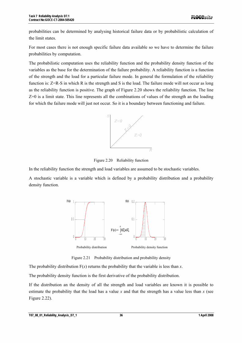
Task 7 Reliability Analysis D7.1 Contract No:GOCE-CT-2004-505420
T07_08_01_Reliability_Analysis_D7_1 36 1 April 2008
probabilities can be determined by analysing historical failure data or by probabilistic calculation of the limit states.
For most cases there is not enough specific failure data available so we have to determine the failure probabilities by computation.
The probabilistic computation uses the reliability function and the probability density function of the variables as the base for the determination of the failure probability. A reliability function is a function of the strength and the load for a particular failure mode. In general the formulation of the reliability function is: Z=R-S in which R is the strength and S is the load. The failure mode will not occur as long as the reliability function is positive. The graph of Figure 2.20 shows the reliability function. The line Z=0 is a limit state. This line represents all the combinations of values of the strength an the loading for which the failure mode will just not occur. So it is a boundary between functioning and failure.
Figure 2.20 Reliability function
In the reliability function the strength and load variables are assumed to be stochastic variables.
A stochastic variable is a variable which is defined by a probability distribution and a probability density function.
F( ) f( )dxx
=−∞∫ ξ ξ
F( x ) f(x)
Probability distribution Probability density function
Figure 2.21 Probability distribution and probability density
The probability distribution F(x) returns the probability that the variable is less than x.
The probability density function is the first derivative of the probability distribution.
If the distribution an the density of all the strength and load variables are known it is possible to estimate the probability that the load has a value x and that the strength has a value less than x (see Figure 2.22).

Task 7 Reliability Analysis D7.1 Contract No:GOCE-CT-2004-505420
T07_08_01_Reliability_Analysis_D7_1 37 1 April 2008
Figure 2.22 Components of the failure probability
The failure probability is the probability that S=x and R<x for every value of x. So we have to compute the sum of the probabilities for all possible values of x:
f P f ( ) F ( )dS Rx x x∞
−∞
= ∫
This method can be applied when the strength and the load are independent of each other.
Figure 2.23 Joint probability density function
Figure 2.23 gives the joint probability density of the strength and the load for a certain failure mode in which the strength and the load are not independent.
The strength is plotted on the horizontal axis and the load is plotted on the vertical axis.
The contours give the combinations of the strength and the load with the same probability density. In the area (Z<0) the value of the reliability function is less then zero and the element will fail.
The failure probability can by determined by summation of the probability density of all the combinations of strength and load in this area.
RS0
P ffZ
(r,s)drds<
= ∫∫
P( ) f ( )dP( ) F ( )
P( ) f ( )F ( )dS x x xR x x
S x R x x x xS
RS R
= =≤ =
⎫⎬⎭⇒ = ∩ ≤ =

Task 7 Reliability Analysis D7.1 Contract No:GOCE-CT-2004-505420
T07_08_01_Reliability_Analysis_D7_1 38 1 April 2008
In a real case the strength and the load in the reliability function are nearly always functions of multiple variables. For instance the load can consist of the water level and the significant wave height. In this case the failure probability is less simple to evaluate. Nevertheless with numerical methods like numerical integration and Monte Carlo simulation it is possible to solve the integral:
1 2 n 1 2 mr ,r ,...,r ,s ,s ,...,s 1 2 1 2 1 2 1 20
P ff n m n mZ
.. (r ,r ,...,r ,s ,s ,...,s )dr dr ...r ds ds ...ds<
= ∫∫ ∫∫
These methods which take into account the real distribution of the variables are called level III probabilistic methods. In the Monte Carlo simulation method a large sample of values of the basic variables is generated and the number of failures is counted. The number of failures equals:
( )( )∑=
=N
jjf gN
11 x
In which N is the total number of simulations. The probability of failure can be estimated by:
NN
P ff ≈
The coefficient of variation of the failure probability can be estimated by:
NPV
fPf
1≈
In which Pf denotes the estimated failure probability.
The accuracy of the method depends on the number of simulations. The relative error made in the simulation can be written as:
f
fNN
PPf −
=ε
The expected value of the error is zero. The standard deviation is given as:
f
f
NPP−
=1
εσ
For a large number of simulations, the error is Normal distributed. Therefore the probability that the relative error is smaller than a certain value E can be written as:
( ) ⎟⎟⎠
⎞⎜⎜⎝
⎛Φ=<
εσε EEP
⎟⎟⎠
⎞⎜⎜⎝
⎛−> 11
2
2
fPEkN
The probability of the relative error E being smaller than kσε now equals Φ(k). For desired values of k and E the required number of simulations is given by:
Requiring a relative error of E = 0.1 lying within the 95 % confidence interval (k = 1.96) results in:

Task 7 Reliability Analysis D7.1 Contract No:GOCE-CT-2004-505420
T07_08_01_Reliability_Analysis_D7_1 39 1 April 2008
⎟⎟⎠
⎞⎜⎜⎝
⎛−> 11400
fPN
The equation shows that the required number of simulations and thus the calculation time depend on the probability of failure to be calculated. Most structures in coastal- and river engineering possess a relatively high probability of failure (i.e. a relatively low reliability) compared to structural elements/systems, resulting in reasonable calculation times for Monte Carlo simulation. The calculation time is independent of the number of basic variables and therefore Monte Carlo simulation should be favoured over the Riemann method in case of a large number of basic variables (typically more than five). Furthermore, the Monte Carlo method is very robust, meaning that it is able to handle discontinuous failure spaces and reliability calculations in which more than one design point are involved (see below).
The problem of long calculation times can be partly overcome by applying importance sampling. This is not elaborated upon here. Reference is made to (Bucher, 1987; Ditlevsen & Madsen, 1996).
If the reliability function (Z) is a sum of a number of normal distributed variables then Z is also a normal distributed variable. The mean value and the standard deviation can easily be computed with these equations:
1
n
i ii
Z a x=
=∑ , 1
i
n
Z i xi
aμ μ=
=∑ , ( )σ σZ i xi
n
ai
==∑
2
1
.
This is the base of the level II probabilistic calculation. The level II methods approximate the distributions of the variables with normal distributions and they estimate the reliability function with a linear first order Taylor polynomial , so that the Z-function is normal distributed.
If the distribution of the Z-function is normal and the mean value and the standard deviation are known it is rather easy to determine the failure probability.
P P( ) ( )f = < = −
=
Z
Z
Z
0 Φ β
β μσ
with:
Figure 2.24 Probability density of the Z-function
By computing β as μ divided by σ it is possible to use the standard normal distribution to estimate
the failure probability.
There are tables available of the standard normal distribution in the handbooks for statistics.
Non linear Z-function
In case of a non linear Z-function it will be estimated with a Taylor polynomial:

Task 7 Reliability Analysis D7.1 Contract No:GOCE-CT-2004-505420
T07_08_01_Reliability_Analysis_D7_1 40 1 April 2008
1
ZZ( ) ( *) ( *)n
i ii i
x Z x x xx
∂∂=
≈ + ⋅ −∑r r
The function is depending of the point where it will be linearised. The mean value and the standard deviation of the linear Z-function can be determined easily. If the reliability function is estimated by a
linear Z-function in the point where all the variable have there mean value ( *ii xx μ= ) we speak of a
Mean Value Approach.
The so-called design point approach estimates the reliability function by a linear function in a point on Z=0 where the joint PDF has a maximum. Finding the design point is a maximisation problem. For this problem there several numerical solutions which will not be discussed here.
Non normally distributed basic variables
If the basic variables of the Z-function are not normally distributed the Z-function will be unknown and probably non normally distributed. To cope with this problem the non normally distributed basic variables in the Z-function can be replaced by a normally distributed variable. In the design point the adapted normal distribution must have the same value as the real distribution. Because the normal distribution has two parameters ( μ and σ ) one condition is not enough to find the right normal
distribution. Therefore the value of the adapted normal probability density function must also have the same value as the real probability density function (see Figure 2.25).
Figure 2.25 Adapted normal distribution
The two conditions give a set of two equations with two unknown which can be solved:
NNxN
xN ,*)(f*)(f*)(F*)(F
σμ⇒⎭⎬⎫
==
xxxx
This method is known as the Approximate Full Distribution Approach (AFDA).

Task 7 Reliability Analysis D7.1 Contract No:GOCE-CT-2004-505420
T07_08_01_Reliability_Analysis_D7_1 41 1 April 2008
3 Preliminary reliability analysis
3.1 PRA for test pilot site Thames
The reliability analysis of the Dartford Creek to Gravesend flood defence system consists of the following steps. Firstly, the floodplain boundaries and main structure types are defined. Secondly, the failure mechanisms of the structure types are specified by means of process models. Thirdly, the flood defence line is discretised into sections that can be represented by one cross section. Finally, the probabilistic calculations are carried out and interpreted. The Dartford Creek to Gravesend flood defence line protects one floodplain and consists of a wide variety of flood defence structures, Figure 3.1.
Figure 3.1 Location of Dartford Creek, Gravesend and the Thames barrier at Greenwich in the Thames Estuary
The reliability analysis includes earth embankments, concrete walls and anchored sheet pile walls. Figure 3.2 shows the main structure types, their site specific failure processes and the failure mechanisms that were taken into account in the reliability analysis. The hydraulic boundary conditions along the Dartford Creek to Gravesend flood defence line are governed by the tidal conditions rather than the fluvial discharges. A Monte Carlo simulation of joint wind speed and tidal water levels at the mouth of the Thames Estuary is combined with iSIS predictions to derive inner estuarial local water levels. A simple predictive model is applied to derive local wave conditions. The soil conditions are generally represented by a clayey peaty layer overlying a water conductive gravel or sand layer.
After the site description the reliability analysis proceeds with the process model definition of the failure mechanisms for each structure type. In order to carry out the probabilistic calculations, the relevant flood defence information needs to be extracted. To this end, the flood defence line is discretised into flood defence sections with similar characteristics. Each flood defence section is represented by one cross section in terms of its geometry, revetment, soil properties, hydraulic boundary conditions etc. The information requirements are determined by the failure mechanisms that are taken into account for the structure type of the flood defence section.
Figure 3.3 and Figure 3.4present fragility curves for earth embankments and reinforced concrete walls. Anchored sheet pile walls are more likely to fail for lower water levels. During a storm with increasing water levels the probability of failure therefore remains equal to the initial failure probability. The probability of failure of the anchored sheet pile wall equals 0.15 due to jointly anchor breaking and rotational failure of the sheet pile wall. The probability of failure does not always cover all the relevant
Swanscombe Marshes
Dartford Creek
25 km N
Thames barrier

Task 7 Reliability Analysis D7.1 Contract No:GOCE-CT-2004-505420
T07_08_01_Reliability_Analysis_D7_1 42 1 April 2008
failure mechanisms or the probability of breach. The probability of failure of earth embankments does not take slope instability into account. The probability of failure of reinforced concrete walls does not take failure of the embankment underneath the concrete wall into account and therefore does not represent the probability of breach. The probability of failure of anchored sheet pile walls represents the probability of ground instability and damage to the assets behind the anchored sheet pile wall.
Flood defence structure type and primary function Site specific failure processes Failure mechanisms in reliability analysis Earth embankments Primary function: flood defence
• Overtopping / overflow causing erosion and slope instability
• Uplifting and piping • Fissuring / cracking • Long term crest level settlements:
compressible layers and estuarial settlements
• Short term crest level settlements: off-road cycling
• Bathymetrical changes of Thames • Third party activities loading
embankment slopes
• (Wave) overtopping and erosion • Combination of uplifting and piping
Concrete walls Primary function: flood defence, in some cases part of larger earth embankment structure
Damage by residential developments: concrete cracking, joint failure and settlements
• Uplifting and piping underneath overall earth embankment (only for types 1 and 2)
• Sliding of the concrete wall • Overturning of the concrete wall • Reinforcement failure in the vertical
concrete slab • Shear failure in the vertical concrete
slab
Anchored sheet pile walls Primary function: ground retaining in frontage previously used as docks
• Accelerated Low Water Corrosion in the splash zone
• Corrosion of the ground anchors
• Breaking of the ground anchor • Sliding of the ground anchor due to
insufficient shear strength of the soil • Breaking of the sheet pile cross section • Rotational failure of the sheet pile after
failure of the ground anchor
Figure 3.2 The Flood defence structure types, their primary function, site specific failure processes and the failure mechanisms which were included in the reliability analysis.
L1
L2
L3
hc
h3
d_a
angl
e
l_l1
l_l2l_l3
l_l4
gamma_s2
gamma_s1
gamma_s3
gamma_s4
gamma_s5
gamma_s6 l_l5
hc1
L
hc2Floodplain
River Thames Impermeable layers
Water conductivesand / gravel layer
1
2
3
Riverward Landward
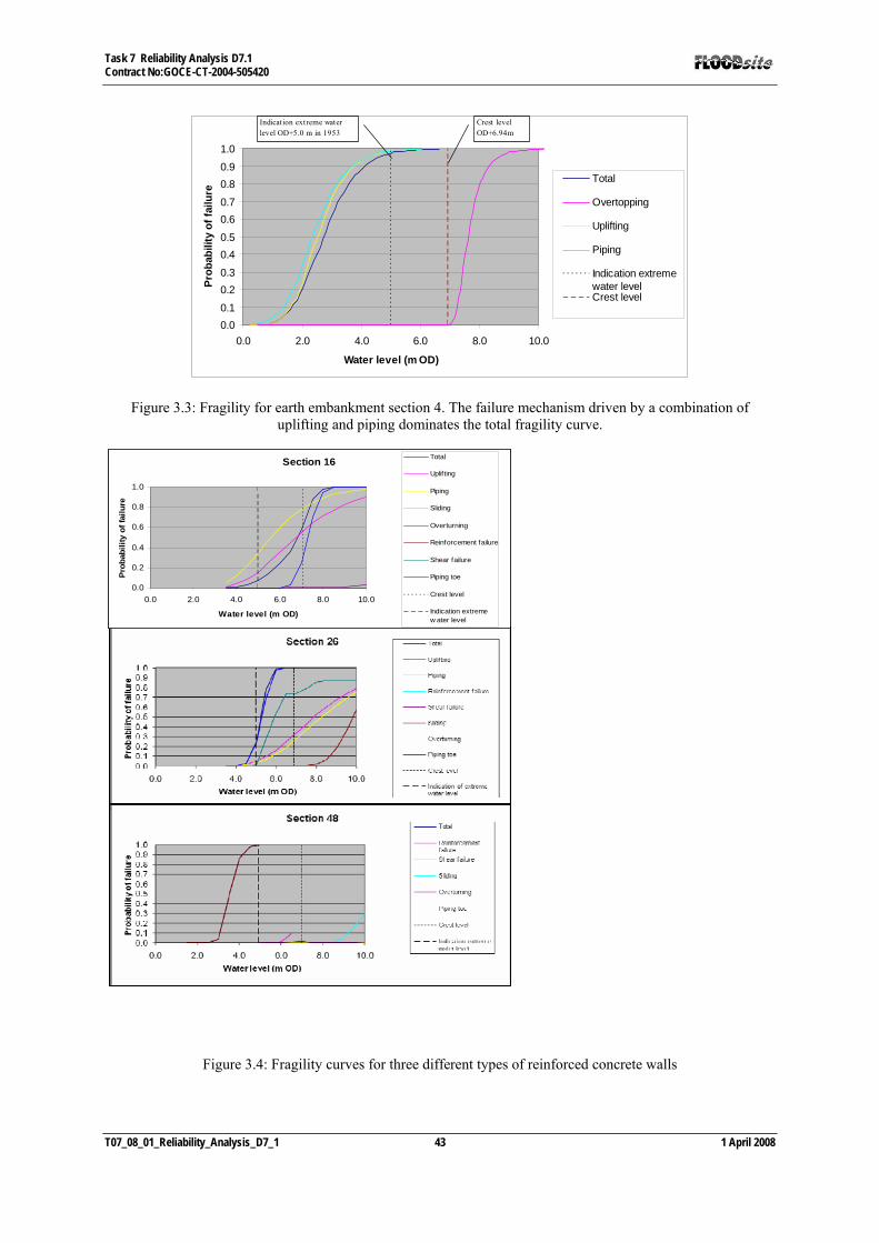
Task 7 Reliability Analysis D7.1 Contract No:GOCE-CT-2004-505420
T07_08_01_Reliability_Analysis_D7_1 43 1 April 2008
0.00.1
0.20.3
0.40.5
0.60.7
0.80.91.0
0.0 2.0 4.0 6.0 8.0 10.0
Water level (m OD)
Prob
abili
ty o
f fai
lure
Total
Overtopping
Uplifting
Piping
Indication extremewater levelCrest level
Indication extreme water level OD+5.0 m in 1953
Crest level OD+6.94m
Figure 3.3: Fragility for earth embankment section 4. The failure mechanism driven by a combination of uplifting and piping dominates the total fragility curve.
Figure 3.4: Fragility curves for three different types of reinforced concrete walls
Section 16
0.0
0.2
0.4
0.6
0.8
1.0
0.0 2.0 4.0 6.0 8.0 10.0
Water level (m OD)
Prob
abili
ty o
f fai
lure
Total
Uplifting
Piping
Sliding
Overturning
Reinforcement failure
Shear failure
Piping toe
Crest level
Indication extremew ater level

Task 7 Reliability Analysis D7.1 Contract No:GOCE-CT-2004-505420
T07_08_01_Reliability_Analysis_D7_1 44 1 April 2008
3.2 PRA for test pilot site Scheldt
This section provides a description of dike ring area 32, Zeeuws-Vlaanderen, and the schematizations of the various dike sections. The assessment of the water board is given in this section as well.
First general information concerning the location and the characteristics of the dike ring is presented followed by an overview of the dikes and structures. Calculations have been made by DHV with checks by VNK and assessments by WZE and are presented at the end of this section.
Location and characteristics
Dike ring area 32 encompasses all of Zeeuw-Vlaanderen with primary embankments of category a, these are embankments that enclose the dike ring areas – either with or without high grounds- and directly retain outside water, along the North Sea and Westerschelde. The length of primary embankments in Zeeuws-Vlaanderen amounts to 85 kilometers, of which 8 kilometers of dune coast. The exceedance frequency for this area equals to 1/4000 years. The dike ring is border-crossing with Belgium. The embankments in Belgium are of category d. Its length is unknown. A system of regional (secondary) embankments is situated at a variable distance from the primary embankments along the whole North Sea coast and Westerschelde.
An overview of the dike ring area is given in figure 2-1.
The dike ring is enclosed by the following embankments:
The dike along the Westerschelde The dike along the Schelde The high grounds in Belgium and Northern France The sea retaining dunes or dikes of Belgium, Northern France and the Netherlands
Dikes, dunes and structures
An overview of the embankments in dike ring 32 is given on the overview map primary and regional embankment of dike ring area 32. The following important water retaining structures can be distinguished:
Dike with stone covering Dike with grass covering Dike with asphalt covering Dune Sea walls RWS (Public Works and Water Management) Engineering structure
The following division can be made:
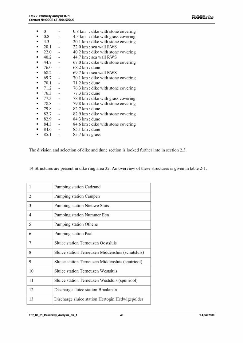
Task 7 Reliability Analysis D7.1 Contract No:GOCE-CT-2004-505420
T07_08_01_Reliability_Analysis_D7_1 45 1 April 2008
0 - 0.8 km : dike with stone covering 0.8 - 4.3 km : dike with grass covering 4.3 - 20.1 km : dike with stone covering 20.1 - 22.0 km : sea wall RWS 22.0 - 40.2 km : dike with stone covering 40.2 - 44.7 km : sea wall RWS 44.7 - 67.0 km : dike with stone covering 76.0 - 68.2 km : dune 68.2 - 69.7 km : sea wall RWS 69.7 - 70.1 km : dike with stone covering 70.1 - 71.2 km : dune 71.2 - 76.3 km : dike with stone covering 76.3 - 77.3 km : dune 77.3 - 78.8 km : dike with grass covering 78.8 - 79.8 km : dike with stone covering 79.8 - 82.7 km : dune 82.7 - 82.9 km : dike with stone covering 82.9 - 84.3 km : dune 84.3 - 84.6 km : dike with stone covering 84.6 - 85.1 km : dune 85.1 - 85.7 km : grass
The division and selection of dike and dune section is looked further into in section 2.3.
14 Structures are present in dike ring area 32. An overview of these structures is given in table 2-1.
1 Pumping station Cadzand
2 Pumping station Campen
3 Pumping station Nieuwe Sluis
4 Pumping station Nummer Een
5 Pumping station Othene
6 Pumping station Paal
7 Sluice station Terneuzen Oostsluis
8 Sluice station Terneuzen Middensluis (schutsluis)
9 Sluice station Terneuzen Middensluis (spuiriool)
10 Sluice station Terneuzen Westsluis
11 Sluice station Terneuzen Westsluis (spuiriool)
12 Discharge sluice station Braakman
13 Discharge sluice station Hertogin Hedwigepolder

Task 7 Reliability Analysis D7.1 Contract No:GOCE-CT-2004-505420
T07_08_01_Reliability_Analysis_D7_1 46 1 April 2008
14 Discharge sluice station Nol Zeven
Table 2.1: Structures in dike ring 32
Division in 33 dike and 4 dune sections
The dike ring area “Zeeuws-Vlaanderen” was initially divided into 287 dike sections according to the VNK-schematization. These were mainly dikes, but encompassed a number of dunes and structures as well. Because calculating the probability of failure for this number of dike sections with PC-Ring is very elaborate, a selection has been made by DHV. This selection is based on the presently existing sections in PC-Ring. Thus no routes with representative dike sections have been selected.
The chosen 33 dike and 4 dune sections are dike ring covering and are deemed to be representative for the total dike ring.
The dike ring area is divided into parts for the selection, each with their own characteristic orientation. One or more dike sections are selected within these parts, where thought is given to the following aspects:
Length of the dike section
Height of the crown
Height of the toe
Orientation of the dike section
Presence of shoulder and/or bend (in other words type of dike section)
Dike covering
The results of the already calculated overflow/wave run-up and bursting/piping of PC-Ring are considered for the choice of dike sections. The dike sections with a significant higher probability of failure have been selected. It was decided to add two more weak links, in consultation with the District Water Board Zeeuws-Vlaanderen. These are dike sections 7009 and 7023. This brings the total number of sections that are taken into account in PC-Ring to 37, of which 33 dike and 4 dune sections. This number is without the water retaining structures (14 structures). The location of the selected dike sections is shown in figure 2-1 (in which dike section 2 represents dike section number 7002 etc). The selected dune sections are given in figure 2-2 (dune section 8 represents dune section number 7008 etc).

Task 7 Reliability Analysis D7.1 Contract No:GOCE-CT-2004-505420
T07_08_01_Reliability_Analysis_D7_1 47 1 April 2008
Figure 2-1 Selected dike sections
Figure 2-2 Selected dune sections
The 33 dike sections are numbered according to the following distances in kilometer :
7002 7009 7023 7024 7025 7028 7038 7042 7047 7053 7071 7074 7075 7094 7109
85.2 82.4 71.7 71.6 71.2 70.1 65.1 64.1 63.6 61.9 57.6 56.9 55.7 51.7 47.4
7111 7116 7124 7129 7136 7139 7152 7159 7163 7167 7185 7202 7211
46.4 45.7 39 36.7 33.3 32 28.2 27.1 25.6 24.2 18.8 14.1 12.6
7220 7233 7249 7258 7271
11.5 8.8 6.4 3.9 0.9
System failure probability of 33 dike- and 4 dune sections
If all results of the component probabilities are taken into consideration, a preliminary probability of flooding of >1/11 per year (COMBIN 1) is calculated for dike ring area 32, Zeeuws-Vlaanderen. This

Task 7 Reliability Analysis D7.1 Contract No:GOCE-CT-2004-505420
T07_08_01_Reliability_Analysis_D7_1 48 1 April 2008
would mean that flooding is to be expected more than once each 11 years for dike ring area 32. Since the results have not been analysed thoroughly, one can not speak of a so-called reference sum of dike ring 32 in this case.
Mechanism COMBIN1 COMBIN2
Overflow / overtopping 1/794 1/11312
Bursting and piping 1/30211 1/30211
Revetment damage and dike erosion
1/22 1/574713
Overflow and overtopping of hydraulic structures
1/16920 1/16920
Non-closure of hydraulic structures
1/3984 1/3984
Structural failures of hydraulic structures
1/22 1/34364
Overall failure probability 1/11 1/1996
Table 4-6 Probability of flooding dike ring 32 according to DHV.
When the 6 weakest spots for the dikes (7167-097-dp290 for overtopping and wave overrun), 7002-072-dp7, 7009-020-dp16, 7028-004-dp25, 7258-074-dp99 and 7271-072-dp69 for covering damaging and erosion body of the dike) and the weakest spot for the structures (constructive failure of pumping station Othene) are left out of consideration, a probability of flooding of 1/2000 per year (COMBIN 2) is calculated. According to the water board this approaches the value it would expect.
In both cases the mechanism sliding is not taken into account in the calculated probability, whilst it is clear that stability problems are a real threat in this case, because the dikes are high and steep and stand on weak layers in the sub-soil.
Because of the reasons a probability of flooding of <1/100 for dike ring area 32 is presented in the main report and the management summary of the project VNK. Herewith it is indicated that the probability of flooding is mainly determined by stability problems at the pumping station or at the dikes. In relation to the pumping station, it is consequently also indicated that this can be approved based on recent information with the second testing.

Task 7 Reliability Analysis D7.1 Contract No:GOCE-CT-2004-505420
T07_08_01_Reliability_Analysis_D7_1 49 1 April 2008
3.3 PRA for test pilot site German Bight
Within Action 3 of Activity 1 a preliminary reliability analysis (PRA) of the pilot site ‘German Bight Coast’ was performed the results of which are summarised in Kortenhaus & Lambrecht (2006). The reliability analysis was performed using the German ‘ProDeich’ model for coastal dikes as described in Kortenhaus (2003) and laser scan data of the flood defences made available by the coastal authorities of Schleswig-Holstein.
This section describes the approach to derive the overall probability of failure for all flood defences in the area. This comprises:
• a description of the flood prone area and the flood defence structures;
• the methodology to obtain geometrical parameters from laser scan measurements of the defence line;
• the development of an algorithm how the defence line can be split into different sections which can be treated independently;
• the calculation of the failure probability for each section of the flood defence line.
The methodology applied here is following the source-pathway-receptor model used in FLOODsite . The result of assessing the risk sources and the risk pathways is the probability of the flood defence failure, as highlighted in this figure.
St. Peter-Ording is a large community at the Schleswig-Holstein North Sea coast with the character of a tourist seaside resort. The community is located on the west (=exposed) coast of Eiderstedt peninsula (Figure 3.6). The size of the study area is approximately 6000 ha; from these about 4000 ha are considered to be flood-prone with the respective height distribution (NN = Ordinance Datum = regional Mean Water Level).

Task 7 Reliability Analysis D7.1 Contract No:GOCE-CT-2004-505420
T07_08_01_Reliability_Analysis_D7_1 50 1 April 2008
Figure 3.5: Map of pilot site ‘German Bight’ (red line illustrates the coastal dike)
The territory of the community amounts to 2800 ha with about 6300 inhabitants. In this area the irregular topography with intermittent small hills and dunes makes it difficult to draw flood-distance boundaries. Presently, flood protection is provided by a major dike (12.5 km long, about 8.0 m high) as well as dune structures 800 m, about 10 m and up to 18.0 m high), surrounding the community on three sides over a length of more than 15 km. The height of the dike line is not constant as shown in Figure 3.7.

Task 7 Reliability Analysis D7.1 Contract No:GOCE-CT-2004-505420
T07_08_01_Reliability_Analysis_D7_1 51 1 April 2008
Figure 3.6: Height of costal defence structures at pilot site ‘German Bight’
Risk sources at the German Bight are resulting from storm surges in the North Sea associated with high water levels and storm waves at the flood defences. Typically, storm surges last not longer than 12 to 24 hours but may increase the water level considerably (up to 3.5 m in the North Sea). The interaction of normal tides (water level differences in the range of 1-2 m are normal in the North Sea region), storm surges, and waves is crucial for the determination of the water level at the coast. In addition, the foreshore topography plays a major role when determining the waves at the flood defence structure. In case of the German Bight the limited water depths over a high foreland will cause the waves to break and will therefore limit the maximum wave heights which reach the flood defence structures. However, the PRA has only considered single probability distributions for each of the governing variables such as water level, wave height and wave period. No joint or conditional probability density functions were considered.
As for risk pathways in the German Bight Coast pilot site, flood defences comprise more than 12 km of dikes (grass and asphalt dike) and a dune area of about 2.5 km length. The PRA has however focussed on the dikes as the key flood defence structure since the dune belt is extraordinary high and wide and is regarded as significantly safer than the dike protection.
Before starting the probabilistic analysis the dike geometry and laser scan data have been used to define different sections of the flood defences. Criteria for distinction of different sections were the type of flood defence, its height, its orientation, the key sea state parameters like water level and waves, and geotechnical parameters. Thirteen sections have been identified using these criteria (see Kortenhaus & Lambrecht, 2006). Each of these sections is assumed to be identical over its entire length and hence will result in the same probability of failure.

Task 7 Reliability Analysis D7.1 Contract No:GOCE-CT-2004-505420
T07_08_01_Reliability_Analysis_D7_1 52 1 April 2008
The PRA has used a full probabilistic approach starting from the input parameters at the toe of the dike and applying early versions of the failure modes and fault trees which have been developed under FLOODsite for the specific type of flood defences. Time dependencies of limit state equations have been considered. Figure 3.8 shows a simplified version of the fault tree used for one of the sections at German Bight Coast for a typical sea dike. Most of the required input parameters for the failure modes are of stochastic nature which means that not only mean or design parameters but also a statistical distribution of this parameter describing the uncertainty is provided. The result of this analysis is an annual probability of flooding of the hinterland for each dike section which has been selected. These flooding probabilities were typically found to range from a probability of 10-4 to 10-6 which means a return period of flooding in the range of 10,000 or 1,000,000 years. The overall flooding probability using a fault tree approach for all sections results in Pf = 4⋅10-3.
Flooding of hinterland5.4⋅10-5
Breach3.1⋅10-6
Wave Overtopping4.0⋅10-5
Overflow1.1⋅10-5
Failure outer slope5.8⋅10-8
Failure dike top< 1.0⋅10-10
Failure inner slope< 1.0⋅10-10
Sliding3.0⋅10-6
Non-structural failure5.1⋅10-5
Figure 3.7: Typical fault tree for a dike section at “German Bight Coast”
The following lessons have been learned from performing this study for the German Bight Coast pilot site:
• The given results should only be used carefully since results depend on variations of parameter settings which still have to be performed.
• A limit state equation for dunes is still missing and needs to be implemented.
• The wide foreland in the German Bight Coast will induce heavy wave breaking under design conditions (and also for lower water levels of course). Results might therefore be dependent on morphodynamic processes and changes of these forelands. Breaker criteria should always be used when waves approaching the structure.
• Updated and harmonised limit state equations are needed to compare reliability calculations of pilot sites to each other.
• A wide range of input parameters are not directly available and had to be estimated. Therefore, sensitivity analyses of the influences of parameters have to be performed.

Task 7 Reliability Analysis D7.1 Contract No:GOCE-CT-2004-505420
T07_08_01_Reliability_Analysis_D7_1 53 1 April 2008
• Criteria for splitting the defence line into various sections need to be automatically derived in the model. Up to now, this is done semi-automatic (with some manual checks of the section at the end). Any change in key parameters of a dike section is therefore not directly leading to a re-calculation of the distinction of all the sections.
• Distinction between different sections was based on the assumption that the sections can be treated independently when calculating the overall failure probability of the system. This still needs verification or improved methods considering the length effect between sections.
• Dependencies between failure mechanisms or scenarios have not been considered yet. A first simple step to consider dependencies might be sensitivity calculations for different degrees of dependencies resulting in a range of possible failure probabilities. However, since the overall failure probability seems mostly dependent on section 8 (overtopping dike) inclusion of dependencies at this stage will probably not influence the result significantly.

Task 7 Reliability Analysis D7.1 Contract No:GOCE-CT-2004-505420
T07_08_01_Reliability_Analysis_D7_1 54 1 April 2008
4 Uncertainty analysis
4.1 Introduction
The reliability of a flood defence system is determined by all the uncertainties that are involved. The aim of this chapter is to provide a systematic overview of all the uncertainties in flood defence systems, as well as to determine the influence of the uncertainties on the reliability of the flood defence system.
The chapter will start with a framework for classification of uncertainties in Section 4.2. Difference can be made between natural variability and knowledge uncertainties. Uncertainties in flood defences are classified according to this framework in Section 4.3. The influence of the several uncertainties (i.e. sensitivity coefficients) will be investigated by means of a few case studies in Section 4.4. The following dike ring areas in the Netherlands are investigated:
• Dike ring area 32: Zeeuwsch Vlaanderen (Influenced by sea and river) • Dike ring area 7: Noordoostpolder (Influenced by a lake) • Dike ring area 36: Land van Heusden / De Maaskant (Influenced by a river)
Dike ring areas in different parts of the Netherlands will be investigated since the dominant failure mechanism tend to be different. River dominated dike rings are influenced differently than sea dominated dike rings. Finally, in Section 4.5 is considered how we could deal with uncertainties.
4.2 Types of uncertainty
Difference can be made between two types of uncertainty. Uncertainty due to the lack of knowledge and uncertainty that stem from known (or observable) populations and therefore represent randomness in samples. The various types of uncertainty are elaborated in this chapter.
4.2.1 Uncertainties
There is no uniform and widely accepted definition of an uncertainty. According to (Sayers et. al., 2002), uncertainties are 'A general concept that reflects our lack of sureness about something, ranging from just short of complete sureness to an almost complete lack of conviction about an outcome.' Uncertainties are introduced in probabilistic risk analysis when we deal with parameters that are not deterministic (exactly known) but that unknown, hence uncertain. These uncertain parameters can be represented by probability density functions. 'In flood risk management there is often considerable difficulty in determining the probability and consequences of important types of event. Most engineering failures arise from a complex and often unique combination of events and thus statistical information on their probability and consequence may be scarce or unavailable' (Floodsite, 2005)
4.2.2 Definitions
Two main groups of uncertainty can be identified:
1. Natural variability: Uncertainties that stem from known (or observable) populations and therefore represent randomness in samples. (Van Gelder, 2000)

Task 7 Reliability Analysis D7.1 Contract No:GOCE-CT-2004-505420
T07_08_01_Reliability_Analysis_D7_1 55 1 April 2008
2. Knowledge uncertainties: Uncertainties that come from basic lack of knowledge of fundamental phenomena. (Van Gelder 2000)
Different terminology is used to describe the same two uncertainties. Many sources use different words, while the intended meaning is more or less the same. Table 4.1 gives an overview of the different terminology. According to Floodsite's 'Language of Risk' (Floodsite, 2005), above mentioned terminology (natural variability and knowledge uncertainty) is used.
Table 4.1: Used terms to describe two types of uncertainty (based on Christian, 2004, Baecher & Christian,2003 and National Research Council,1995)
Natural variability Knowledge uncertainty
Uncertainty due to naturally variable phenomena in time or space
Uncertainty due to lack of knowledge or understanding of nature
inherent uncertainty Epistemic uncertainty
Aleatory uncertainty
Natural variability Knowledge uncertainty
Random or random variability Functional uncertainty
Objective uncertainty Subjective uncertainty
External uncertainty Internal uncertainty
Statistical uncertainty Inductive probability
Chance Probability
Natural variability can be subdivided in natural variability in time and natural variability in space. Knowledge uncertainties can be subdivided in model uncertainty and statistical uncertainty; statistical uncertainty can be subdivided in parameter and distribution type uncertainty (Van Gelder, 2000). The different groups of uncertainty are elaborated in the subsequent sections.

Task 7 Reliability Analysis D7.1 Contract No:GOCE-CT-2004-505420
T07_08_01_Reliability_Analysis_D7_1 56 1 April 2008
Figure 4.1: Classification of uncertainties, after Van Gelder (2000)
4.2.3 Natural variability
4.2.3.1 General
Natural variability can be defined as: Uncertainties that stem from known (or observable) populations and therefore represent randomness in samples, see section 4.2.2. In other words, natural variability "represent randomness or the variations in nature" (Van Gelder, 2000). For example, one cannot predict the maximum water level that will at a certain location along the coast next year. There are many realisations possible. Christian (2003) compares natural variability with throwing a dice. The dice is so unpredictable that additional knowledge or analysis will not affect our ability to predict it. One important property of natural variability is that it cannot be reduced by for instance more measurements. Two types of uncertainty can be distinguished: natural variability in time and natural variability in space.
4.2.3.2 Natural variability in time
Random processes running in time (individual wave heights, significant wave heights, water levels, discharges, etc.) are examples of the class of natural variability in time. Unlimited data will not reduce this uncertainty. The realisations of the process in the future remain uncertain. The probability density function (PDF) or the cumulative probability distribution function (CDF) and the auto-correlation function describe the process.
In case of a periodic stationary process like a wave field the autocorrelation function will have a sinusoidal form and the spectrum, as the Fourier-transform of the autocorrelation function, gives an adequate description of the process. Attention should be paid to the fact that the well known wave energy spectra as Pierson-Moskowitz and Jonswap are not always able to represent the wave field at a
Uncertainty
Knowledge
Natural variability
Model
Statistical
Time
Space
Parameter
Distribution

Task 7 Reliability Analysis D7.1 Contract No:GOCE-CT-2004-505420
T07_08_01_Reliability_Analysis_D7_1 57 1 April 2008
site. In quite some practical cases, swell and wind wave form a wave field together. The presence of two energy sources may be clearly reflected in the double peaked form of the wave energy spectrum.
An attractive aspect of the spectral approach is that the natural variability can be easily transferred through linear systems by means of transfer functions. By means of the linear wave theory the incoming wave spectrum can be transformed into the spectrum of wave loads on a flood defence structure. The PDF of wave loads can be derived from this wave load spectrum. Of course it is assumed here that no wave breaking takes place in the vicinity of the structure. In case of non-stationary processes, that are governed by meteorological and atmospheric cycles (significant wave height, river discharges, etc.) the PDF and the autocorrelation function are needed. Here the autocorrelation function gives an impression of the persistence of the phenomenon. The persistence of rough and calm conditions is of utmost importance in workability and serviceability analyses.
If the interest is directed to the analysis of ultimate limit states e.g. sliding of the structure, the autocorrelation is eliminated by selecting only independent maxima for the statistical analysis. If this selection method does not guarantee a set of homogeneous and independent observations, physical or meteorological insights may be used to homogenise the dataset. For instance if the fetch in NW-direction is clearly maximal, the dataset of maximum significant wave height could be limited to NW-storms. If such insight fails, one could take only the observations exceeding a certain threshold (POT) into account hoping that this will lead to the desired result. In case of a clear yearly seasonal cycle the statistical analysis can be limited to the yearly maxima.
Special attention should be given to the joint occurrence of significant wave height Hs and spectral peak period Tp. A general description of the joint PDF of Hs and Tp is not known. A practical solution for extreme conditions considers the significant wave height and the wave steepness sp as independent random variables to describe the dependence. This is a conservative approach as extreme wave heights are more easily realised than extreme peak periods. For the practical description of daily conditions (service limit state: SLS) the independence of sp and Tp seems sometimes a better approximation. Also the dependence of water levels and significant wave height should be explored because the depth limitation to waves can be reduced by wind set-up. Here the statistical analysis should be clearly supported by physical insight. Moreover it should not be forgotten that shoals could be eroded or accreted due to changes in current or wave regime induced by the construction of the flood defence structure.
4.2.3.3 Natural variability in space
When determining the probability distribution of a random variable that represents the variation in space of a process (like the fluctuation in the height of a dike), there essentially is a problem of shortage of measurements. It is usually too expensive to measure the height or width of a dike in great detail. This statistical uncertainty of variations in space can be reduced by taking more measurements (Vrijling and Van Gelder, 1998). Whether the variations of for instance soil properties are to be classified as natural variability or as knowledge uncertainties is not unambiguous, see section 4.2.3.4.
Soil properties can be described as random processes in space. From a number of field tests the PDF of the soil property and the (three-dimensional) autocorrelation function can be fixed for each homogeneous soil layer. Here the theory is further developed than the practical knowledge. Numerous

Task 7 Reliability Analysis D7.1 Contract No:GOCE-CT-2004-505420
T07_08_01_Reliability_Analysis_D7_1 58 1 April 2008
mathematical expressions are proposed in the literature to describe the autocorrelation. No clear preference has however emerged yet as to which functions describe the fluctuation pattern of the soil properties best. Moreover, the correlation length (distance where correlation becomes negligible) seems to be of the order of 30 to 100m while the spacing of traditional soil mechanical investigations for flood defence structures is of the order of 500m. So it seems that the intensity of the soil mechanical investigations has to be increased considerably if reliable estimates have to be made of the autocorrelation function.
The acquisition of more data has a different effect in case of random processes in space than in time. As structures are immobile, there is only one single realisation of the field of soil properties. Therefore the soil properties at the location could be exactly known if sufficient soil investigations were done. Consequently the actual soil properties are fixed after construction, although not completely known to man. The uncertainty can be described by the distribution and the autocorrelation function, but it is in fact a case of lack of info.
4.2.3.4 Remarks natural variability in space
One of the 'traditional' discussion points is the classification of uncertainties in soil properties. According to Van Gelder (2000) and Van der Most & Wehrung (2005), soil properties are natural variability in space. According to Christian (2004), soil properties are knowledge uncertainties. Both approaches can be defended since uncertainties from soil properties stem from spatial variation (natural variability) and sample and laboratorial variations (knowledge). Besides, spatial variation can be regarded as both inherent and epistemic uncertainties. Basically, it is a lack of knowledge, measuring the soil exactly on every single location will result in perfect knowledge of the soil (excluding sample and laboratorial uncertainties), however, this is practically not feasible.
4.2.4 Knowledge uncertainties
4.2.4.1 General
Knowledge uncertainties were defined as uncertainties that come from basic lack of knowledge of fundamental phenomena, see section 4.2.2. In other words, " Knowledge uncertainties are caused by lack of knowledge of all the causes and effects in physical systems, or by lack of sufficient data. For example, it might only be possible to obtain the type of the distribution, or the exact model of a physical system, when enough research could and would be done." (Van Gelder, 2000). There is usually one, or a limited amount, of realisations in case of knowledge uncertainties. Christian (2003) compares knowledge uncertainty with a pack of shuffled cards. The arrangement of the cards is fixed but unknown. The arrangement could be discovered by examining each single card, but this is usually (in other cases than a deck of cards) not possible. The strategy is usually to measure and induce from these measurement to discover the arrangement. This is actually done in case of the card-game 'Bridge'. One important property of knowledge uncertainties is that they may change as knowledge increases. Knowledge uncertainties can be subdivided model uncertainty and statistical uncertainty; statistical uncertainty can be subdivided in parameter and distribution type uncertainty.
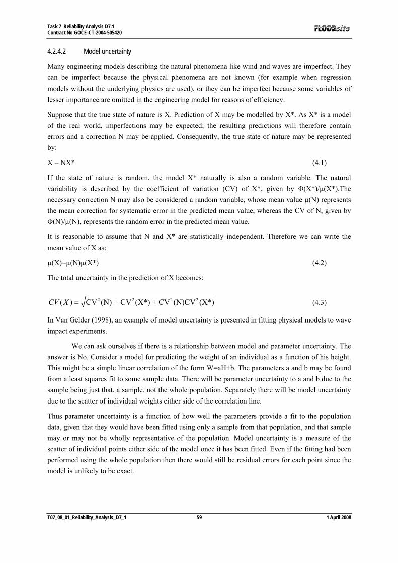
Task 7 Reliability Analysis D7.1 Contract No:GOCE-CT-2004-505420
T07_08_01_Reliability_Analysis_D7_1 59 1 April 2008
4.2.4.2 Model uncertainty
Many engineering models describing the natural phenomena like wind and waves are imperfect. They can be imperfect because the physical phenomena are not known (for example when regression models without the underlying physics are used), or they can be imperfect because some variables of lesser importance are omitted in the engineering model for reasons of efficiency.
Suppose that the true state of nature is X. Prediction of X may be modelled by X*. As X* is a model of the real world, imperfections may be expected; the resulting predictions will therefore contain errors and a correction N may be applied. Consequently, the true state of nature may be represented by:
X = NX* (4.1)
If the state of nature is random, the model X* naturally is also a random variable. The natural variability is described by the coefficient of variation (CV) of X*, given by Φ(X*)/µ(X*).The necessary correction N may also be considered a random variable, whose mean value µ(N) represents the mean correction for systematic error in the predicted mean value, whereas the CV of N, given by Φ(N)/µ(N), represents the random error in the predicted mean value.
It is reasonable to assume that N and X* are statistically independent. Therefore we can write the mean value of X as:
µ(X)=µ(N)µ(X*) (4.2)
The total uncertainty in the prediction of X becomes:
2 2 2 2( ) CV (N) + CV (X*) + CV (N)CV (X*)CV X = (4.3)
In Van Gelder (1998), an example of model uncertainty is presented in fitting physical models to wave impact experiments.
We can ask ourselves if there is a relationship between model and parameter uncertainty. The answer is No. Consider a model for predicting the weight of an individual as a function of his height. This might be a simple linear correlation of the form W=aH+b. The parameters a and b may be found from a least squares fit to some sample data. There will be parameter uncertainty to a and b due to the sample being just that, a sample, not the whole population. Separately there will be model uncertainty due to the scatter of individual weights either side of the correlation line.
Thus parameter uncertainty is a function of how well the parameters provide a fit to the population data, given that they would have been fitted using only a sample from that population, and that sample may or may not be wholly representative of the population. Model uncertainty is a measure of the scatter of individual points either side of the model once it has been fitted. Even if the fitting had been performed using the whole population then there would still be residual errors for each point since the model is unlikely to be exact.

Task 7 Reliability Analysis D7.1 Contract No:GOCE-CT-2004-505420
T07_08_01_Reliability_Analysis_D7_1 60 1 April 2008
Parameter uncertainty can be reduced by increasing the amount of data against which the model fit is performed. Model uncertainty can be reduced by adopting a more elaborate model (e.g. quadratic fit instead of linear). There is, however, no relationship between the two.
4.2.4.3 Statistical uncertainty: parameter
This uncertainty occurs when the parameters of a distribution are determined with a limited number of data. The smaller the number of data, the larger the parameter uncertainty. A parameter of a distribution function is estimated from the data and thus a random variable. The parameter uncertainty can be described by the distribution function of the parameter. In Van Gelder (1996) an overview is given of the analytical and numerical derivation of parameter uncertainties for certain probability models (Exponential, Gumbel and Log-normal). The bootstrap method is a fairly easy tool to calculate the parameter uncertainty numerically. Given a dataset x=(x1,x2,...,xn), we can generate a bootstrap sample x* which is a random sample of size n drawn with replacement from the dataset x. The following bootstrap algorithm can be used for estimating the parameter uncertainty:
1. Select B independent bootstrap samples x*1, x*2, ..., x*B, each consisting of n data values drawn with replacement from x.
2. Evaluate the bootstrap corresponding to each bootstrap sample θ*(b)=f(x*b) for b=1,2,...,B (4.4)
3. Determine the parameter uncertainty by the empirical distribution function of θ*. The algorithm has been applied in Van Gelder (1996) to the location parameter A and scale parameter B of the Gumbel distribution with a Maximum Likelihood fit to the Hook of Holland data. The parameter uncertainty could be very well approximated by normal distributions with coefficient of variations of around 10%.
Other methods to model parameter uncertainties like Bayesian methods can be applied too (Van Gelder, 1996). Bayesian inference lays its foundations upon the idea that states of nature can be and should be treated as random variables. Before making use of data collected at the site the engineer can express his information concerning the set of uncertain parameters θ for a particular model f(x|θ), which is a PDF for the random variable x. The information about θ can be described by a prior distribution μ(θ|I), i.e. prior to using the observed record of the random variable x. Non-informative priors can be used if we don’t have any prior information available. If p(2) is a non-informative prior, consistency demands that p(Η)dΗ=p(2)d2 for Η=Η(2); thus a procedure for obtaining the ignorance prior should presumably be invariant under one-to-one reparametrisation. A procedure which satisfies this invariance condition is given by the Fisher matrix of the probability model:
2
| 2( ) log ( | )xI E f xθθ θθ
⎡ ⎤∂= − ⎢ ⎥∂⎣ ⎦ (4.5)
giving the so-called non-informative Jeffrey’s prior p(θ)=I(θ)1/2.

Task 7 Reliability Analysis D7.1 Contract No:GOCE-CT-2004-505420
T07_08_01_Reliability_Analysis_D7_1 61 1 April 2008
The engineer now has a set observations x of the random variable X, which he assumes comes from the probability model fX(x|). Bayes’ theorem provides a simple procedure by which the prior distribution of the parameter set may be updated by the dataset X to provide the posterior distribution of , namely,
( | , ) ( | ) ( | ) /f X I l X I Kθ θ π θ= (4.6)
where
f(θ|X,I) posterior density function for , conditional upon a set of data X and information I;
l(X|θ) sample likelihood of the observations given the parameters
π(θ|I) prior density function for , conditional upon the initial information I
K normalizing constant (K=Σl(X|θ)π(θ|I))
The posterior density function of is a function weighted by the prior density function of and the data-based likelihood function in such a manner as to combine the information content of both. If future observations XF are available, Bayes’ theorem can be used to update the PDF on . In this case the former posterior density function for now becomes the prior density function, since it is prior to the new observations or the utilization of new data. The new posterior density function would also have been obtained if the two samples X and XF had been observed sequentially as one set of data. The way in which the engineer applies his information about depends on the objectives in analyzing the data. The Bayesian methods will be described in more detail in Section 3.
4.2.4.4 Statistical uncertainty: distribution type
This type represents the uncertainty of the distribution type of the variable. It is for example not clear whether the occurrence of the water level of the North Sea is exponentially or Gumbel distributed or whether it has another distribution. A choice was made to divide statistical uncertainty into parameter- and distribution type uncertainty although it is not always possible to draw the line; in case of unknown parameters (because of lack of observations), the distribution type will be uncertain as well.
Any approach that selects a single model and then makes inference conditionally on that model ignores the uncertainty involved in the model selection, which can be a big part in the overall uncertainty. This difficulty can be in principle avoided , if one adopts a Bayesian approach and calculates the posterior probabilities of all the competing models following directly from the Bayes factors. A composite inference can then be made that takes account of model uncertainty in a simple way with the weighted average model:
1 1 2 2( ) ( ) ( ) ... ( )n nf h f h f h f hθ θ θ= + + + (4.7)
where 1i
θ =∑ .
4.2.5 Correlations between uncertainties
Correlations between parameters play an important role in the determination of the reliability of a flood defence systems. The main influence of uncertainties is on system scale, individual failure mechanisms and dike sections are less affected by correlations. Correlations may be present in both

Task 7 Reliability Analysis D7.1 Contract No:GOCE-CT-2004-505420
T07_08_01_Reliability_Analysis_D7_1 62 1 April 2008
the load on the system and in the resistance of the system (Vrouwenvelder, 2006). Difference can be made between correlations in time and correlations in space.
4.2.5.1 Correlation functions
There are several types of correlation functions, for more information about correlation functions is referred to Meermans (1997). The computer program PC-Ring that is used in this study (Steenbergen and Vrouwenvelder, 2003A) uses the following correlations functions:
Correlation in space
Correlations in space mainly affect the resistance (or strength) parameters. Spatial correlations are modelled in PC-RING with an autocorrelation function (Vrouwenvelder, 2006):
2
2
( ) (1 ) x
xd
x xx eρ ρ ρΔ−
Δ = + − ⋅ (4.8)
where ( )xρ Δ Correlation between two points of consideration
xΔ Distance between two points of consideration
xρ Constant correlation
2
xd Correlation distance
Correlation in time
A model developed by Borges and Castanheta can be used to take correlations in time into account. See Vrouwenvelder (2006) for more infotmation how the Borges-Castanheta model is incorporated in PC-RING. Discrete time intervals are being used to model time series of for instance water levels. Full correlation applies within the time interval; a constant correlation applies between the several intervals (usually 0) Correlations in time mainly affect the load parameters. Figure 4.2 shows how a time series of water levels can be modelled according to the Borges-Castanheta model.
Figure 4.2: Borges-Castanheta model for the combination of river and sea induced water levels (Vrouwenvelder, 2006)
Uncertainties about correlations

Task 7 Reliability Analysis D7.1 Contract No:GOCE-CT-2004-505420
T07_08_01_Reliability_Analysis_D7_1 63 1 April 2008
The correlations itself are not certain either, since they are usually estimated by expert judgement or after the analysis of datasets. The correlation function parameters can be represented by probability density functions (pdf); these pdf's can be incorporated in the calculations procedures. This makes the calculation procedure more difficult and time consuming. There, uncertainties about correlations are usually neglected.

Task 7 Reliability Analysis D7.1 Contract No:GOCE-CT-2004-505420
T07_08_01_Reliability_Analysis_D7_1 64 1 April 2008
4.3 Classification of uncertainties
A classification of uncertainties is provided in this chapter in order to obtain insight in the properties of all the uncertainties.
4.3.1 General overview
A general overview of uncertainties that are involved in flood defence is provided by Van Der Most and Wehrung (2005). The uncertainties are split in natural variability and in knowledge uncertainties, see Table 4.2.
Table 4.2: General classification uncertainties based on Van der Most and Wehrung (2005)
Type Source
Categories of uncertainty Hydraulic loads Strength of water defences
Natural variability Natural variation Temporal variation of discharges, waves and water levels
Spatial variation of soil properties
Future developments /policies
Climate change, Space for river policy
Knowledge uncertainties
Lack of data (statistical uncertainty)
Probabilistic model of discharges, waves and water levels
Characteristics of dikes and subsoil, idem structures
Lack of knowledge (model uncertainty)
Mathematical models for water levels and waves
Mathematical models for failure mechanisms
Aging of dikes, structures
4.3.2 Probability of failure of a dike
To obtain all uncertainties in flood defences, all the failure mechanisms that contribute to the probability of failure of the flood defence have to be investigated. The probability of failure of a dike ring is determined by the probability of failure of the individual dike sections (a dike ring is usually 'cut' in sections that have more or less equal properties). The relation between the probability of failure of a dike section and the failure mechanisms can be shown with a failure tree, see Figure 4.3.

Task 7 Reliability Analysis D7.1 Contract No:GOCE-CT-2004-505420
T07_08_01_Reliability_Analysis_D7_1 65 1 April 2008
Figure 4.3: Failure tree of a flood defences (Lassing et al, 2003)
4.3.3 Failure mechanisms
The computer program PC-RING (Steenbergen and Vrouwenvelder, 2003A; Lassing et al, 2003) was developed to calculate the probability of failure of a flood defence system. Several assumptions had to be made regarding the failure mechanisms. Not all failure mechanisms contribute equally to the probability of failure of a flood defence. The following failure mechanism have been assumed to be the dominant mechanisms (Steenbergen and Vrouwenvelder, 2003B):
• Overflow/overtopping • Slope instability • Heave/piping • Erosion revetment and erosion dike body • Piping structures • Not closing structures • Dune erosion
4.3.4 Classification
All the uncertainties (represented by the pdf of the random variables) that appeared in section 4.3.3 can be classified according to the division of Section 4.2, see Table 4.3. The classification must be interpreted as a rough attempt since some uncertainties could be classified in different groups.
There are different considerations possible about classification of uncertainties. The classification mentioned in section 4.3.4 reflects an initial attempt to start building correspondence
Table 4.3: Classification of uncertainties
Natural variability Knowledge uncertainties
in time in space model Statistical
parameter distribution type

Task 7 Reliability Analysis D7.1 Contract No:GOCE-CT-2004-505420
T07_08_01_Reliability_Analysis_D7_1 66 1 April 2008
Natural variability Knowledge uncertainties
in time in space model Statistical
parameter distribution type
Dike height
Toe height
Angle outer slope (top)
Angle outer slope (bottom)
Angle inner slope
Berm height
Berm width
Geo
met
ry
Error in determination ground level
Layer thickness (Clay layer inner slope)
Model factor critical overflow discharge
Roughness inner slope
Factor for determination Qb
Model factor for occurring overflow
discharge
Cohesion (Clay layer inner slope)
Factor for determination Qn
Friction angle (Clay layer inner slope)
Ove
rtop
ping
/ ov
erflo
w
Soil density (Clay layer inner slope)
Model uncertainty Bishop
Deviation water levels
cohesion per layer
Slop
e st
abili
ty
friction angle per layer
Thickness covering layer
Model factor heave Apparent relative density of heaving
soil
Inner water level Model factor piping Relative soil density sand (grain)
Leakage length Model factor water level (damping)
Factor Cbear
Thickness sand layer Uniformity
rolling resistance angle
Grain size
White's constant
heav
e/pi
ping
Specific permeability

Task 7 Reliability Analysis D7.1 Contract No:GOCE-CT-2004-505420
T07_08_01_Reliability_Analysis_D7_1 67 1 April 2008
Natural variability Knowledge uncertainties
in time in space model Statistical
parameter distribution type
Width covering clay layer
Coefficient erosion covering layer
Width dike core at crest height
Coefficient erosion dike core
Angle outer slope Acceleration factor erosion rate
Angle inner slope Declination erosion speed
Reve
tmen
t - g
ener
al
Angle in reduction factor r
Root depth grass
Gra
ss Coefficient grass
Stone pitching thickness
Relative density stone pitching
Ston
e pi
tchi
ng -
no fi
lter
Coefficient stone pitching on clay
Stone pitching thickness
Relative density stone pitching
Thickness granular filter layer
Grain size 15% percentile filer
Crack width
Coefficient stone pitching on filter
Coefficient in determination leakage length
Ston
e pi
tchi
ng -
filte
r
Coefficient in determination
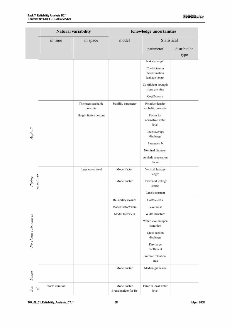
Task 7 Reliability Analysis D7.1 Contract No:GOCE-CT-2004-505420
T07_08_01_Reliability_Analysis_D7_1 68 1 April 2008
Natural variability Knowledge uncertainties
in time in space model Statistical
parameter distribution type
leakage length
Coefficient in determination leakage length
Coefficient strength stone pitching
Coefficient c
Thickness asphaltic concrete
Stability parameter Relative density asphaltic concrete
Height fictive bottom Factor for normative water
level
Level average discharge
Parameter b
Nominal diameter
Asph
alt
Asphalt penetration factor
Inner water level Model factor Vertical leakage length
Model factor Horizontal leakage length
Pipi
ng
stru
ctur
es
Lane's constant
Reliability closure Coefficient c
Model factorVkom Level raise
Model factorVin Width structure
Water level in open condition
Cross section discharge
Discharge coefficient
No
clos
ure
stru
ctur
es
surface retention area
Dun
es Model factor Median grain size
Loa d
Storm duration Model factor Bretschneider for Hs
Error in local water level

Task 7 Reliability Analysis D7.1 Contract No:GOCE-CT-2004-505420
T07_08_01_Reliability_Analysis_D7_1 69 1 April 2008
Natural variability Knowledge uncertainties
in time in space model Statistical
parameter distribution type
Model factor Bretschneider for Ts
Deviation wave direction
Water level Maasmond Parameter magnitude
discharge Lobith
Wind speed Parameter slope discharge Lobith
Discharge Lobith (Rijn) Parameter h North Sea
Water level Delfzijl Parameter Tp North Sea
Water level OS11 Parameter Hs North Sea
Water level Dalfsen (Vecht)
Parameter wind ν
Discharge Olst (IJssel) Parameter wind θ
Discharge Lith (Maas)
Prediction error water level Maeslantkering
Water level IJsselmeer
Water level Markermeer
Water level Hoek van Holland
Water level Den Helder
Water level Vlissingen
Water level Harlingen
Water level Lauwersoog
Wind speed Schiphol / Deelen
Wind speed 'ligth island' Goeree
Wind speed de Kooy
Wind speed Vlissingen
Wind speed Terschelling West
Prediction error water level
Oosterscheldekering
Load
s
Duration wind setup

Task 7 Reliability Analysis D7.1 Contract No:GOCE-CT-2004-505420
T07_08_01_Reliability_Analysis_D7_1 70 1 April 2008
Natural variability Knowledge uncertainties
in time in space model Statistical
parameter distribution type
Phase difference
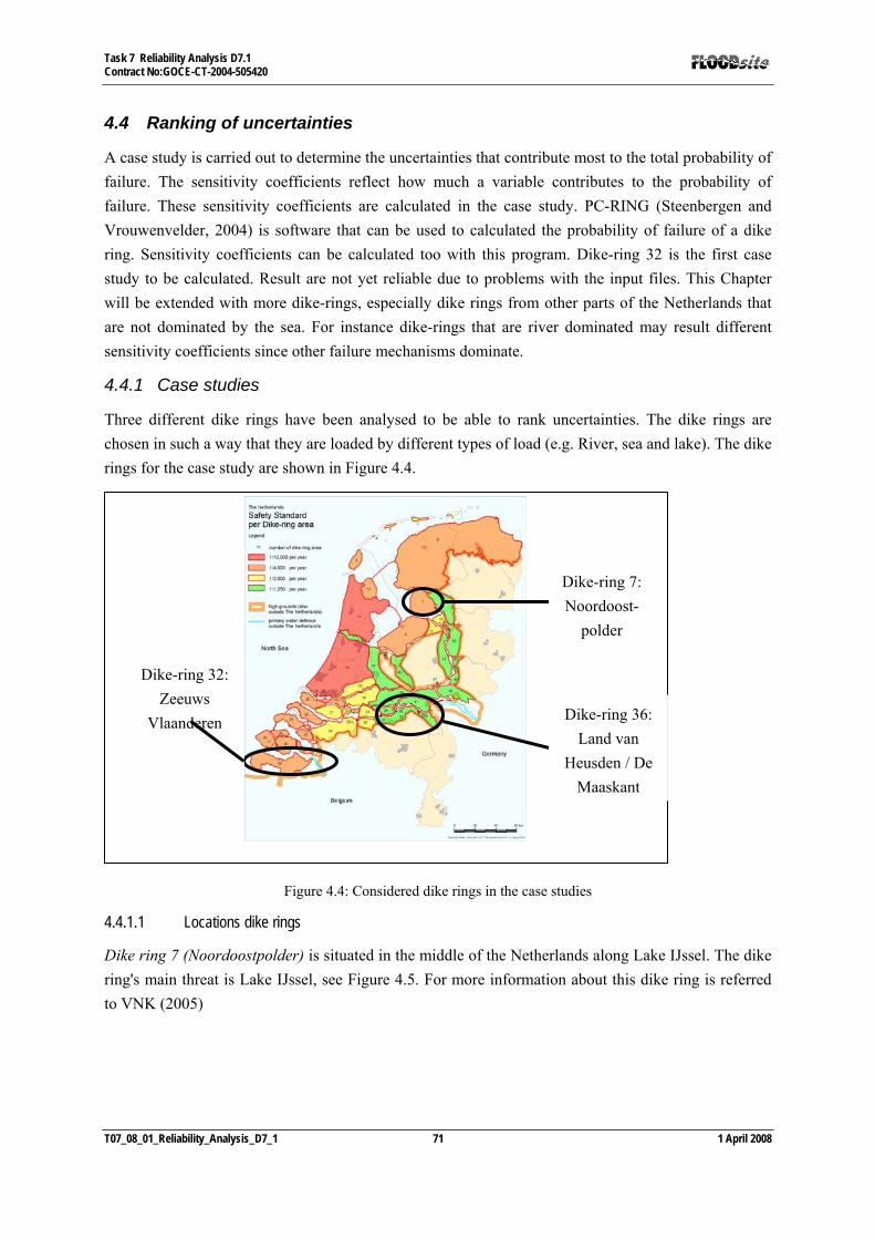
Task 7 Reliability Analysis D7.1 Contract No:GOCE-CT-2004-505420
T07_08_01_Reliability_Analysis_D7_1 71 1 April 2008
4.4 Ranking of uncertainties
A case study is carried out to determine the uncertainties that contribute most to the total probability of failure. The sensitivity coefficients reflect how much a variable contributes to the probability of failure. These sensitivity coefficients are calculated in the case study. PC-RING (Steenbergen and Vrouwenvelder, 2004) is software that can be used to calculated the probability of failure of a dike ring. Sensitivity coefficients can be calculated too with this program. Dike-ring 32 is the first case study to be calculated. Result are not yet reliable due to problems with the input files. This Chapter will be extended with more dike-rings, especially dike rings from other parts of the Netherlands that are not dominated by the sea. For instance dike-rings that are river dominated may result different sensitivity coefficients since other failure mechanisms dominate.
4.4.1 Case studies
Three different dike rings have been analysed to be able to rank uncertainties. The dike rings are chosen in such a way that they are loaded by different types of load (e.g. River, sea and lake). The dike rings for the case study are shown in Figure 4.4.
Figure 4.4: Considered dike rings in the case studies
4.4.1.1 Locations dike rings
Dike ring 7 (Noordoostpolder) is situated in the middle of the Netherlands along Lake IJssel. The dike ring's main threat is Lake IJssel, see Figure 4.5. For more information about this dike ring is referred to VNK (2005)
Dike-ring 32: Zeeuws
Vlaanderen
Dike-ring 7: Noordoost-
polder
Dike-ring 36: Land van
Heusden / De Maaskant

Task 7 Reliability Analysis D7.1 Contract No:GOCE-CT-2004-505420
T07_08_01_Reliability_Analysis_D7_1 72 1 April 2008
Figure 4.5: Dike ring 7: Noordoostpolder
Dike-ring 32 (Zeeuws Vlaanderen) is situated in the south-west of the Netherlands, bordering Belgium in the south. The dike ring is threatened by the North sea in the west and by the Scheldt estuary in the north, see Figure 4.6. For more information about dike ring 32 is referred to VNK (2005)
Figure 4.6: Dike-ring 32: Zeeuws Vlaanderen
Dike ring 36 is situated in the south of the Netherlands. The dike ring's main threats is the river Meuse, see Figure 4.7. For more information about this dike ring is referred to VNK (2005)
Figure 4.7: Dike ring 36: Land van Heusden / De Maaskant
north sea
Scheldt
Western Scheldt estuary
dike ring 32
Meuse
Lake IJssel

Task 7 Reliability Analysis D7.1 Contract No:GOCE-CT-2004-505420
T07_08_01_Reliability_Analysis_D7_1 73 1 April 2008
4.4.1.2 Dominant failure mechanism
The initial calculations with PC-ring show that the 3 considered dike rings have different dominant failure mechanisms. This dominant failure mechanisms are summarized in Table 4.4. For more details is referred to VNK (2005A, 2005B,2005C)
Table 4.4: Dominant failure mechanisms of the considered dike rings
Dike ring number
name main threat dominant failure mechanism
7 Noordoostpolder Lake Hydraulic structures (e.g. sluices)
32 Zeeuws Vlaanderen Sea - river Erosion revetment + hydraulic structures (stability)
36 Land van Heusden / De Maaskant
River Piping
4.4.2 Sensitivity coefficients case studies
The sensitivity coefficients that are the result of a FORM analysis show the relative contribution of an uncertainty. The dike ring mentioned in the previous sections are analyses to obtain the sensitivity coefficients. It must be noted that the used data is preliminary data of part 1 of the FLORIS project (FLORIS, 2006), the project is still improving its datasets and more accurate results are expected in the future. Especially the results of dike ring 32 should be considered as an first indication since the report (FLORIS, 2005B) notes that many problems occurred during calculations. Nonetheless, the calculations still provide a good indication of the relative contribution of the uncertainties.
Calculations have been made with PC-RING (Steenbergen and Vrouwenvelder, 2004) to obtain the sensitivity coefficients. Both sensitivity coefficients (alfa) and the squares of the sensitivity coefficients (alfa^2) are given; the squared values give the relative contribution to the total and are summed equal to 1.0. Table 4.5 shows the 5 most important sensitivity coefficients of dike ring 7 (hence, the five with the highest alfa^2) and Table 4.6 shows the most important sensitivity coefficients of dike ring 32. The result of dike ring 32 are not shown below since the sensitivity coefficients of the load parameters could not be retrieved.
Table 4.5: Highest sensitivity coefficient dike ring 7: Noordoostpolder
variable
number
description alfa alfa^2
19 Wind speed Schiphol/Deelen -0.862 0.743044
20 (null) -0.373 0.139129
18 Level Lake IJssel -0.328 0.107584

Task 7 Reliability Analysis D7.1 Contract No:GOCE-CT-2004-505420
T07_08_01_Reliability_Analysis_D7_1 74 1 April 2008
12 Model factor overflow discharge m_qo -0.057 0.003249
8 Model factor critical overflow discharge m_qc 0.052 0.002704
Table 4.6: Highest sensitivity coefficients dike ring 36: Land van Heusden / De Maaskant
variable number
description alfa alfa^2
19 Discharge Lobith* -0.906 0.820836
20 Discharge Lith* -0.251 0.063001
31 White's constant 0.192 0.036864
22 (null) -0.161 0.025921
35 Model factor piping 0.114 0.012996
* Dike ring 36 is not threatened by the river Rhine (which is measured in Lobith), but due to the structure of the load models in PC-Ring, the discharge (of the Rhine) in Lobith plays a fictive role. In
fact the squared alfa value for the river Meuse should be 2 2 2Meuse Lith Lobithα α α= + .

Task 7 Reliability Analysis D7.1 Contract No:GOCE-CT-2004-505420
T07_08_01_Reliability_Analysis_D7_1 75 1 April 2008
4.4.3 Ranking of uncertainties
The uncertainties that contribute most to the total probability of failure are evaluated in this section.
4.4.3.1 Uncertainties that contribute most
Table 4.5 and Table 4.6 show that the only a few parameters are responsible for almost all the uncertainty. In case of dike ring 7, the highest contribution is due to the wind speed. In dike ring 36, the highest contribution is due to the river Meuse's discharge. Hence, the relative contribution of the uncertainties differ from time to time. In both case studies, there is one dominant uncertainty.
4.4.3.2 Small/mid/large ranking
At the start of this study, it was intended to give a ranking of uncertainties in small (alfa^2 < 1/3) mid (1/3 < alfa < 2/3) and large uncertainties (alfa^2 > 2/3). However, in the three case studies this appeared to be impossible. One reason is that the highest sensitivity coefficients differ from case to case, the other reason is the case studies show only a few variables that form almost 99% of the uncertainty. These variables are predominantly natural variability in time. Because of the high dependency on local circumstances, we cannot infer general conclusions about the ranking of uncertainties.

Task 7 Reliability Analysis D7.1 Contract No:GOCE-CT-2004-505420
T07_08_01_Reliability_Analysis_D7_1 76 1 April 2008
4.5 Dealing with uncertainties
After identifying all uncertainties in Chapter 3 and classifying the main uncertainties in Chapter 4, it is discussed in this chapter how we could deal with the uncertainties.
4.5.1 Effects of uncertainties
All uncertainties in flood defences have been classified in Section 4.3, ranking the uncertainties in probabilistic risk analysis of flood defences in knowledge uncertainties and in natural variability. We have to take into account that uncertainties due to natural variability may not be reduced, while the knowledge uncertainties might be reduced. The uncertainties with the largest impact have been identified in Section 4.4, showing that a few uncertainties are of major importance. The way how could be dealt with these uncertainties is discussed in this Chapter. It is now possible to make a cost benefit analysis to be able to predict which uncertainties are economically viable to reduce. Of course this is only possible for our group of knowledge uncertainties. Two aspects are of importance when considering uncertainty reduction:
• The reduction of risk due to uncertainty reduction (Reduction of uncertainties with high sensitivity coefficients will result in the highest risk reduction)
• The cost of risk reduction (Some knowledge might require more extensive research or measurements than others)
Based on this approach, it is possible to find an optimal uncertainty reduction.
4.5.2 Reduction of uncertainty
In Section 4.2, it was mentioned that natural variability represent randomness or variations in nature. This natural variability cannot be reduced. Knowledge uncertainties, on the other hand, are caused by lack of knowledge. Knowledge uncertainties may change as knowledge increases. In general there are three ways to increase knowledge:
- Gathering data
- Research
- Expert judgement
Data can be gathered by taking measurements or by keeping record of a process in time. Research can, for instance, be undertaken with respect to the physical model of a phenomenon or into the better use of existing data. By using expert opinions, it is possible to acquire the probability distributions of variables that are too expensive or practically impossible to measure.
The goal of all this research obviously is to reduce the uncertainty in the model. Nevertheless it is also thinkable that uncertainty will increase. Research might show that an originally flawless model actually contains a lot of uncertainties. Or after taking some measurements the variations of the dike height can be a lot larger. It is also thinkable that the average value of the variable will change because of the research that has been done.

Task 7 Reliability Analysis D7.1 Contract No:GOCE-CT-2004-505420
T07_08_01_Reliability_Analysis_D7_1 77 1 April 2008
The consequence is that the calculated probability of failure will be influenced by future research. In order to guarantee a stable and convincing flood defence policy after the transition, it is important to understand the extent of this effect. The effect of uncertainty reduction is elaborated in section 4.5.3.
4.5.2.1 Influence of uncertainties on parameters and models to be used in Floodsite
As can be seen in Table 4.5 and Table 4.6, the load parameters contribute most to the total probability of failure. Unfortunately, these uncertainties could be ranked as natural variability, hence reduction of the uncertainty is not possible.
It was also concluded from the case studies that the highest contribution of uncertainty (sensitivity coefficient) differs from case to case. In case we deal with a probabilistic risk analysis that is dominated by knowledge uncertainties (hence reducible), we can increase this knowledge to reduce the probability of failure. How the reduction of uncertainty influences the reliability is discussed in section 4.5.3.
4.5.3 Remaining uncertainties of the reliability index
Until here, we have classified uncertainties, tried to determine the most important ones and discussed methods to reduce the uncertainties. Finally, we can establish the effect of uncertainties and of uncertainty on the reliability of the flood defence. A study performed by Slijkhuis et. al (1999) clearly shows the effect of uncertainty reduction the distribution of the reliability index. Four options for uncertainty reduction are assumed; Option 1: No uncertainties are reduced; Option 4: all uncertainties except the natural variability in time are reduced; Options 2 and 3 involve 'intermediate' reduction of uncertainties. The result is shown in Figure 4.8.
Figure 4.8: Influence uncertainty reduction on distribution reliability index after Slijkhuis et. al. (1999)
This study shows that 'the more uncertainty is expected to be reduced, the higher the mean and the larger the standard deviation of the distribution of the reliability index will be' (Slijkhuis et. al., 1999)

Task 7 Reliability Analysis D7.1 Contract No:GOCE-CT-2004-505420
T07_08_01_Reliability_Analysis_D7_1 78 1 April 2008
4.5.4 How to deal with uncertainties
Finally, we discuss we could deal with uncertainties in probabilistic risk analysis. If we are involved with calculating the expected probability distribution for a random variable X, then the inferences we make on X should reflect the uncertainty in the parameters θ. In the Bayesian terminology we are interested in the so-called predictive function:
( ) ( | ) ( )F x F x f dθ
θ θ θ= ∫ (4.9)
where F(x| θ) is the probabilistic model of X, conditional on the parameters θ and F(x) is the predictive distribution of the random variable x, now parameter free. In popular words: “the uncertainty in the θ parameters has to be integrated out”.
The predictive distribution can be interpreted as being the distribution F(x| θ) weighted by f(θ). In making inferences on a random variable it is important to use the predictive function for x, as opposed to the probabilistic model for x with some estimator for the parameter set θ, i.e. f(x| θ *). This is because using point estimators for uncertain parameters underestimates the variance in the random variable X.
4.5.4.1 Example
The above mentioned techniques will be illustrated with an exponential distribution:
( ) 1x
F x eξ
α−−
= − x ξ≥ (4.10)
The influence of statistical uncertainty in the shift parameter ξ will be considered by writing ξ as ξ + ε , in which , ε ~ N(0,σξ). The PDF of , is given by:
2
221( )2
f e ζ
εσ
ζ
εσ π
−
= (4.11)
According to Eqn. 5.3 , we can write:
2 2
2 2
22 2 2 22 2 2
2 2
12 2 2 2
1 1( ) ( | ) ( ) (1 ) 12 2
11 1 12
x x
xx x
F x F x f d e e d e e d
e e d e e e e
ζ ζ
ζ ζ ζ ζζ
ε ε εζ ε ζασ σα α
ζ ζ
σ σ σ ζ σζ ζεασα α α α α
ζ
ε ε ε ε εσ π σ π
εσ π
− − −− −− −
⎛ ⎞− +⎜ ⎟− −− −− − −⎜ ⎟
⎝ ⎠
= = − = − =
− = − = −
∫ ∫ ∫
∫
(4.12)

Task 7 Reliability Analysis D7.1 Contract No:GOCE-CT-2004-505420
T07_08_01_Reliability_Analysis_D7_1 79 1 April 2008
Notice that the probability of exceedance curve is translated with 2
22ζσ
α .
Now we will consider the influence of statistical uncertainty in the scale parameter. For that purpose
we rewrite the CDF as ( )( ) 1 ax bF x e− −= − . Note that a=1/α and b=ξ/α. Assume a statistical uncertainty
in the a parameter: a=a+ε , in which , ε~N(0,σa). Then:
( )( )( | ) 1 a x bF x e εε − + −= − (4.13)
and
2
221( )2
a
a
f eεσε
σ π
−
= (4.14)
So:
( )( ) ( )2
2 2
( ) /( )2
1( ) ( | ) ( ) 1
2
a
a
a x b
xax b
a
eF x F x f d e d e e
ε ε σσε ε ε ε
σ π
+ −− − −
−= = = −∫ ∫ (4.15)
This can be written again in terms of ξ and α like:
( ){ }2 21/ 2 /( ) 1 ax x
F x eζ σ α α− − −
= − (4.16)
Note that σa = σ (1/α) = f(σα) is difficult to express as a function of Φ∀. The approximation σ (1/α) ≈ 1/σ(α) may not be used. However the relation CV(1/α) ≈ CV(α) is quite good. We therefore use as a first approximation σa= σα/α2. Substitution in Eqn. 5.8 leads to:
( ){ }( )2 2
2 232 2
4
1/ 2/
1/ 2 /2( ) 1 1 1a
x xxx
x xF x e e e e
αζ σ αα σζαζ σ α α α α
⎧ ⎫− −⎪ ⎪−⎨ ⎬ −−− − − ⎪ ⎪⎩ ⎭= − = − = − ⋅ (4.17)
Notice that the probability of exceedance is translated as a function of σa and x. So apart from a shift also the slope of the survival function 1-F increases. Summarizing these results leads to the following Table 4.7:
Table 4.7: Multiplication factors
Exponential Distribution Shift Parameter Scale Parameter
Multiplication Factor
2
22eζσ
α
2 2
42
x
eασ
α
From Table 4.7, we notice the influence of the x-value in the multiplication factor for the scale parameter. The influence of the x-value in the multiplication factor for the shift parameter has disappeared.

Task 7 Reliability Analysis D7.1 Contract No:GOCE-CT-2004-505420
T07_08_01_Reliability_Analysis_D7_1 80 1 April 2008
Summarized; if F(x) = 1 - e-(x-ξ)/α has an uncertainty in the scale parameter (given by σα which should be not too large), then in making inferences on X the original exponential distribution should be “replaced” by Eqn. 4.17.
The equation 4.17 is applied to the data set of extreme water levels at Hook of Holland. This set can be modelled with an exponential distribution with parameters A=1.96 and B=0.33. Different levels of uncertainty in B will be discerned: σB = 0.17, σB = 0.11, and σB = 0.05. The influence of the uncertainty is depicted in Figure 4.9 and appears to be quite large in this particular case study. Notice the combination of translation and rotation of the frequency curves.
2 2 .5 3 3 .5 4 4 .5 51 0
-4
1 0-3
1 0-2
1 0-1
1 00
W a te r le ve l [m ]
Exc
eeda
nce
prob
abili
ty
S ta tis tica l unce rta inty a t va rio us le ve ls
Figure 4.9: Translation and rotation of the frequency curves as σB increases from 5%, 11% to 17%
Uncertainty and sensitivity analyses are similar in that both strive to evaluate the variation in results arising from the variations in the assumptions, models, and data. However, they differ in scope, and the information they provide.
Uncertainty analysis attempts to describe the likelihood for different size variations and tends to be more formalized than sensitivity analysis. An uncertainty analysis explicitly quantifies the uncertainties and their relative magnitudes, but requires probability distributions for each of the random variables. The assignment of these distributions often involves as much uncertainty as that to be quantified.
Sensitivity analysis is generally more straightforward than uncertainty analysis, requiring only the separate (simpler) or simultaneous (more complex) changing of one or more of the inputs. Expert judgement is involved to the extent that the analyst decides which inputs to change, and how much to change them. This process can be streamlined if the analyst knows which variables have the greatest effect upon the results. Variation of inputs one at a time is preferred, unless multiple parameters are affected when one is changed. In this latter case, simultaneous variation is required. For more information about sensitivity analysis is referred to Van Gelder (2000).

Task 7 Reliability Analysis D7.1 Contract No:GOCE-CT-2004-505420
T07_08_01_Reliability_Analysis_D7_1 81 1 April 2008
4.6 Conclusions
Uncertainties are introduced in probabilistic risk analysis when we deal with parameters that are not deterministic (exactly known) but that are unknown instead, hence uncertain. Two groups of uncertainties can be distinguished:
1. Natural variability (Uncertainties that stem from known (or observable) populations and therefore represent randomness in samples)
2. Knowledge uncertainties (Uncertainties that come from basic lack of knowledge of fundamental phenomena)
Natural variability cannot be reduced, while knowledge uncertainties may be reduced. Natural variability can be subdivided in natural variability in time and natural variability in space. Knowledge uncertainty can be subdivided in model uncertainty and statistical uncertainty; statistical uncertainty can be subdivided in parameter uncertainty and in distribution type uncertainty.
An initial attempt is made to rank all uncertainties that are introduced in a probabilistic risk analysis. This list is not unambiguous because several uncertainties could be ranked in more groups. There is still discussion in literature about variability in space, for instance soil properties. On one hand this spatial distribution of properties are mainly a case of lack of knowledge since there is only one realisation of the subsoil. On the other hand, it is practically impossible to reduce all uncertainty, resulting in a remaining (natural) variability. One advantage of uncertainty classification is that clearly can be seen which uncertainties might be reduced (knowledge uncertainties) and which ones not (natural variability).
The influence of uncertainties on the reliability flood defences is investigated in three case studies. Three dike rings are examined and the sensitivity coefficients are calculated. These sensitivity show how much on variable contributes to the total probability of failure. Three different hydraulic regimes apply to the case study areas: one dike ring is mainly influences by sea, one mainly by a lake and one mainly by rivers. The case studies show it is not possible to rank the uncertainties, since the dominant uncertainties (hence high sensitivity coefficients) differ from location to location. Nonetheless, the load parameters seem to be dominant in the case studies. These load parameters are natural variability and therefore not reducible.
Finally, methods are discussed to deal with uncertainties. Knowledge uncertainties can be reduced by performing research (improving models), by gathering data or by expert judgement. Reducing uncertainties have the following effect on the reliability: 'the more uncertainty is expected to be reduced, the higher the mean and the larger the standard deviation of the distribution of the reliability index will be' (Slijkhuis et. al., 1999).
4.7 Database of uncertainties for models and parameters
(Please see Appendix 5.)
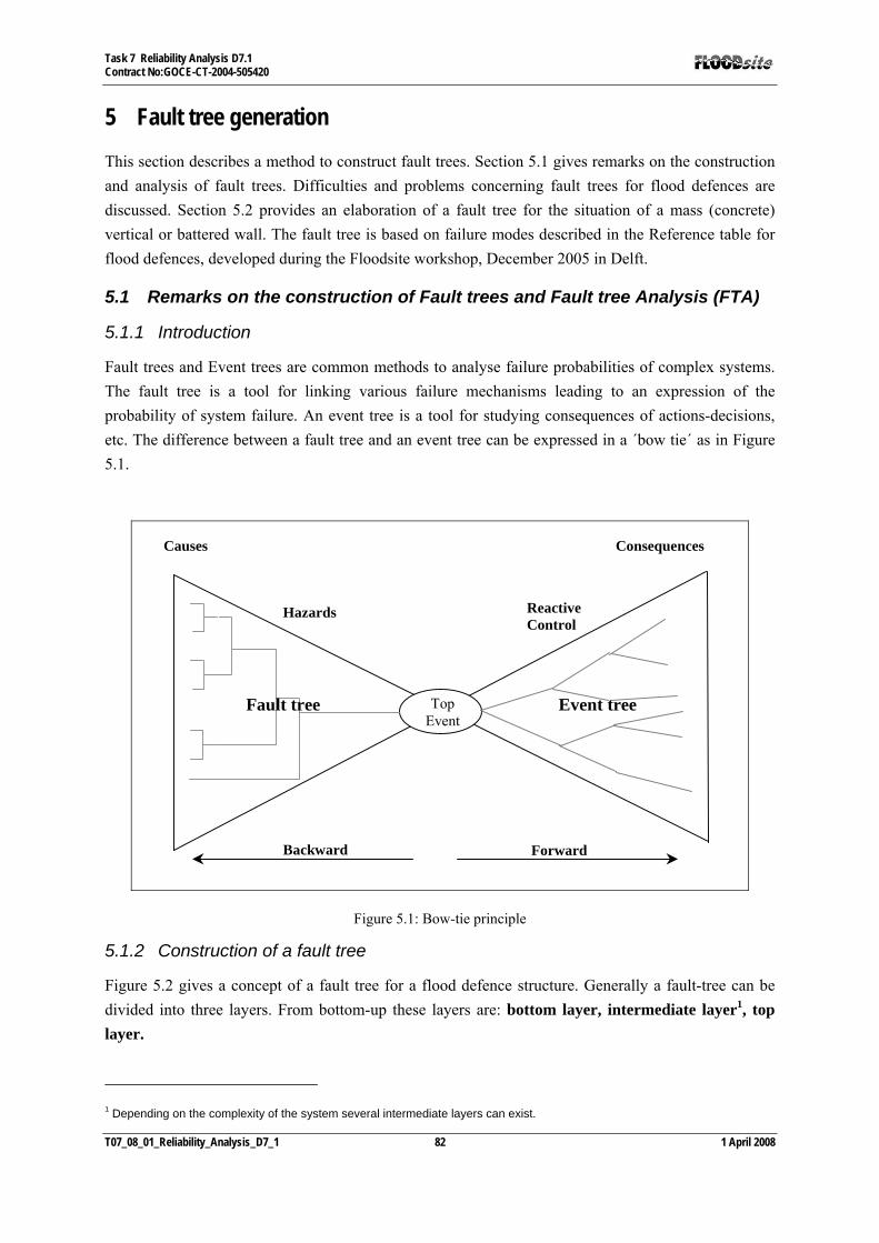
Task 7 Reliability Analysis D7.1 Contract No:GOCE-CT-2004-505420
T07_08_01_Reliability_Analysis_D7_1 82 1 April 2008
5 Fault tree generation This section describes a method to construct fault trees. Section 5.1 gives remarks on the construction and analysis of fault trees. Difficulties and problems concerning fault trees for flood defences are discussed. Section 5.2 provides an elaboration of a fault tree for the situation of a mass (concrete) vertical or battered wall. The fault tree is based on failure modes described in the Reference table for flood defences, developed during the Floodsite workshop, December 2005 in Delft.
5.1 Remarks on the construction of Fault trees and Fault tree Analysis (FTA)
5.1.1 Introduction
Fault trees and Event trees are common methods to analyse failure probabilities of complex systems. The fault tree is a tool for linking various failure mechanisms leading to an expression of the probability of system failure. An event tree is a tool for studying consequences of actions-decisions, etc. The difference between a fault tree and an event tree can be expressed in a ´bow tie´ as in Figure 5.1.
Causes
Top Event
Fault tree Event tree
Consequences
ReactiveControl
Hazards
Backward Forward
Figure 5.1: Bow-tie principle
5.1.2 Construction of a fault tree
Figure 5.2 gives a concept of a fault tree for a flood defence structure. Generally a fault-tree can be divided into three layers. From bottom-up these layers are: bottom layer, intermediate layer1, top layer.
1 Depending on the complexity of the system several intermediate layers can exist.

Task 7 Reliability Analysis D7.1 Contract No:GOCE-CT-2004-505420
T07_08_01_Reliability_Analysis_D7_1 83 1 April 2008
The bottom layer exists of basic events or/and component failure. A basic event is for example the impact of a ship or other human failure, which can be quantified with a certain failure probability (i.e. 3,4·10-6 per year). Component failure corresponds with failure of one of the components of the flood defence structure due to a certain failure (sub)mechanism. At this point the fault tree is fed with a (physical) model, describing the failure (sub)mechanism. Based on a model and data (i.e. soil parameters, hydraulic parameters, uncertainty, etc.) the failure probability of the component due to the (sub)mechanism can be determined. The failure probability can be determined by solving the Limit State Function, which is indicated by the subtext: R < S. Subsequently the results of the bottom layer is a set of failure probabilities.
The intermediate layer describes the several subsystems of the fault tree. In case of a flood defence structure these subsystems will correspond with the several failure mechanisms of the structure.
The top layer combines the failure probabilities of the several failure mechanisms into a overall failure probability of the structure.
5.1.3 Difficulties and problems concerning fault trees for flood defences
Fault trees originate from the aircraft industry and are subsequently used in chemical industry and computer industry. Fault trees are used to create insight in large complex systems with a large amount of components and elements, like computers and aircrafts. The emphasis lies on identifying all possible causes (basic events) of all failure events and to label failure probabilities to these basic events.
Tree size
When applying fault trees on flood defence structures, the emphasis lies more on ‘Where to stop?’ In order to find the right elaboration of a fault tree the following ‘rules’ could be helpful:
- Stop when a mechanism cannot be divided into sub mechanisms. Find the right model to describe the mechanism.
- Do not implement Basic Events or Component Failures when no data is available or when proper quantification is impossible.
- Do not implement events which are unlikely to occur.
In other words: ‘Analyse no further down than is necessary to enter probabilistic data with confidence’
Description of events
As mentioned above Basic Events are tagged with a failure probability. This means that the events should be described as clearly and ‘digital’ as possible. ‘Digital’ means that there are two states: failure and non-failure. An example of a good description is: ‘Drainage system failure’. An example of a bad description is: ‘Groundwater flow behind structure’. This description can be made ‘digital’: ‘Groundwater flow > critical flow velocity’
MOE’s and MOB’s and Dependency

Task 7 Reliability Analysis D7.1 Contract No:GOCE-CT-2004-505420
T07_08_01_Reliability_Analysis_D7_1 84 1 April 2008
A MOE is a Multiple Occurring Event and a MOB is a Multiple Occurring Branch. Both can occur within a fault tree. A MOE can for example be the water level exceeding a critical value or drainage system failure. MOE’s and MOB’s should be handled with care because they create dependency between two (sub)mechanisms. Dependency should be taken into account when calculating the overall failure probability of a flood defence structure.
Cross-references
Cross references make fault trees more complex and can lead to circular-references. For example (see Fault tree Single Crest Embankment): Piping depends on Seepage. Seepage depends on too much settlement. Too much settlement depends again on piping. For simplicity sake cross-references should be minimized.
Pictures
Fault trees should be accompanied with pictures describing the underlying (sub)mechanisms.

Task 7 Reliability Analysis D7.1 Contract No:GOCE-CT-2004-505420
T07_08_01_Reliability_Analysis_D7_1 85 1 April 2008
Figure 5.2: Fault-tree with different layers
Mod
el /
Dat
a Data layer: Geometry – Soil Parameters – Hydraulic Parameters – Stochastic Parameters
Model layer: Applied models (Piping, Overtopping, Instability, etc)
External Structural
Inundation
Terror. Human.
Fail
Animal
activity
Port (OR/AND)
Failure Failure Failure
Port (OR/AND)
Submechanism A
Submechanism B
R < S R < S
R < S
Non structural
Port (OR/AND)
Failure Failure
Port (OR/AND)
Submechanism A
Submechanism B
R < S R < S
R < S
Failure
Bot
tom
Laye
r
Inte
rmed
iate
Laye
r
Top
Laye
r
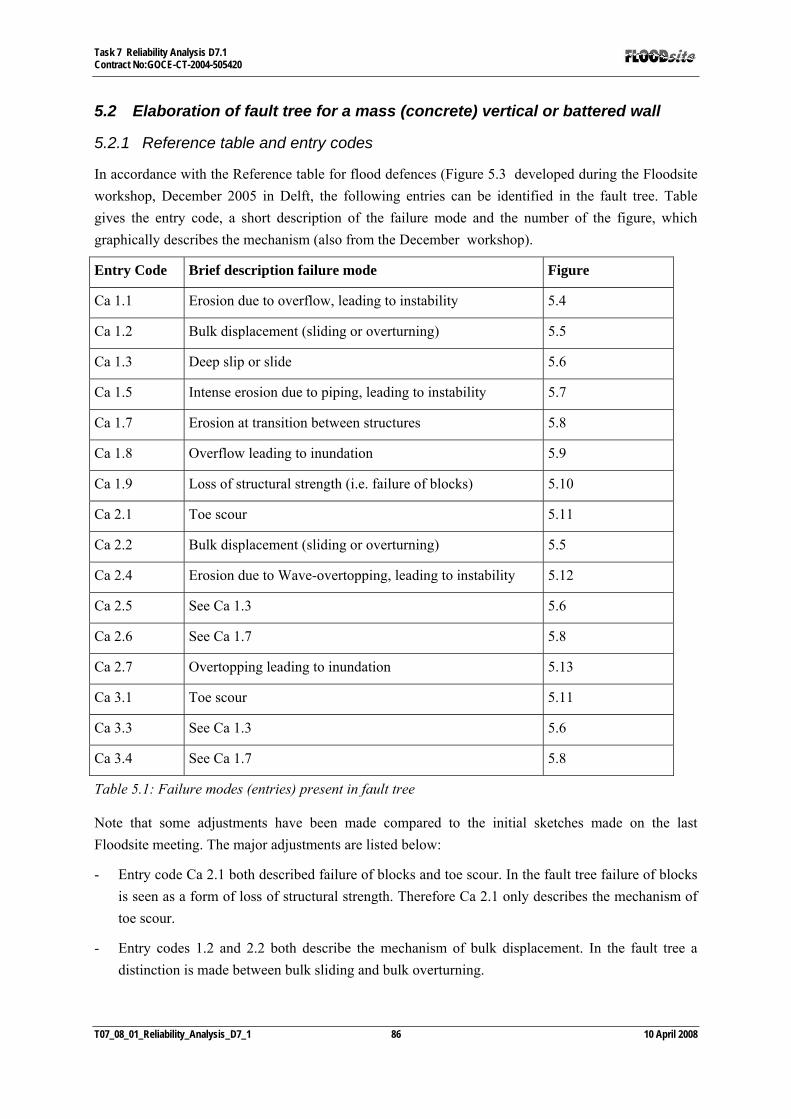
Task 7 Reliability Analysis D7.1 Contract No:GOCE-CT-2004-505420
T07_08_01_Reliability_Analysis_D7_1 86 10 April 2008
5.2 Elaboration of fault tree for a mass (concrete) vertical or battered wall
5.2.1 Reference table and entry codes
In accordance with the Reference table for flood defences (Figure 5.3 developed during the Floodsite workshop, December 2005 in Delft, the following entries can be identified in the fault tree. Table gives the entry code, a short description of the failure mode and the number of the figure, which graphically describes the mechanism (also from the December workshop).
Entry Code Brief description failure mode Figure
Ca 1.1 Erosion due to overflow, leading to instability 5.4
Ca 1.2 Bulk displacement (sliding or overturning) 5.5
Ca 1.3 Deep slip or slide 5.6
Ca 1.5 Intense erosion due to piping, leading to instability 5.7
Ca 1.7 Erosion at transition between structures 5.8
Ca 1.8 Overflow leading to inundation 5.9
Ca 1.9 Loss of structural strength (i.e. failure of blocks) 5.10
Ca 2.1 Toe scour 5.11
Ca 2.2 Bulk displacement (sliding or overturning) 5.5
Ca 2.4 Erosion due to Wave-overtopping, leading to instability 5.12
Ca 2.5 See Ca 1.3 5.6
Ca 2.6 See Ca 1.7 5.8
Ca 2.7 Overtopping leading to inundation 5.13
Ca 3.1 Toe scour 5.11
Ca 3.3 See Ca 1.3 5.6
Ca 3.4 See Ca 1.7 5.8
Table 5.1: Failure modes (entries) present in fault tree
Note that some adjustments have been made compared to the initial sketches made on the last Floodsite meeting. The major adjustments are listed below:
- Entry code Ca 2.1 both described failure of blocks and toe scour. In the fault tree failure of blocks is seen as a form of loss of structural strength. Therefore Ca 2.1 only describes the mechanism of toe scour.
- Entry codes 1.2 and 2.2 both describe the mechanism of bulk displacement. In the fault tree a distinction is made between bulk sliding and bulk overturning.

Task 7 Reliability Analysis D7.1 Contract No:GOCE-CT-2004-505420
T07_08_01_Reliability_Analysis_D7_1 87 10 April 2008

Task 7 Reliability Analysis D7.1 Contract No:GOCE-CT-2004-505420
T07_08_01_Reliability_Analysis_D7_1 88 10 April 2008
Figure 5.3: Reference table for flood defences

Final Report: Theme 1 Task 7 Contract No:GOCE-CT-2004-505420
T07_08_01_Reliability_Analysis_D7_1 89 10 April 2008
5.2.2 Graphical representations of failure modes
This section provides the graphical representations of the failure modes based on sketches made during the December Floodsite workshop.
Figure 5.4: Erosion due to overflow, leading to instability
Figure 5.5: Bulk displacement (sliding or overturning)

Final Report: Theme 1 Task 7 Contract No:GOCE-CT-2004-505420
T07_08_01_Reliability_Analysis_D7_1 90 10 April 2008
Figure 5.6: Deep slip / slide
Figure 5.7: Intense erosion due to piping, leading to instability
Figure 5.8: Erosion at transition between structures

Final Report: Theme 1 Task 7 Contract No:GOCE-CT-2004-505420
T07_08_01_Reliability_Analysis_D7_1 91 10 April 2008
Figure 5.9: Overtopping leading to inundation
Figure 5.10: Loss of structural strength

Final Report: Theme 1 Task 7 Contract No:GOCE-CT-2004-505420
T07_08_01_Reliability_Analysis_D7_1 92 10 April 2008
Figure 5.11: Toe scour
Figure 5.12: Erosion due to wave-overtopping, leading to instability
Figure 5.13: Wave-overtopping leading to inundation

Final Report: Theme 1 Task 7 Contract No:GOCE-CT-2004-505420
T07_08_01_Reliability_Analysis_D7_1 93 10 April 2008
5.2.3 Fault tree of a mass (concrete) vertical or battered wall
This section provides the fault tree of a mass (concrete) vertical or battered wall. The top event (inundation) can be caused by two major events: Breach and Non structural failure.
Breach
A breach can be the result of a number of events. First a breach can be created by bulk displacement (sliding or overturning) of the structure or an element. A breach can also be the result of structural failure or erosion at the transition between structures. Finally, the breach can be a result of instability of the structure. Instability can have a lot of causes: erosion due to overflow or wave-overtopping, piping, a deep slip or toe scour.
Non structural failure In case of non structural failure such a large amount of water enters the area behind the flood defence that this flood defence fails to fulfil the requirements concerning its water retaining function. Nevertheless the structure withstands the hydraulic load. Non structural failure can be the results of both overflow and wave-overtopping. Other causes are: ice dams and piping.
Figure 5.14 gives the fault tree for a mass (concrete) vertical or battered wall.

Final Report: Theme 1 Task 7 Contract No:GOCE-CT-2004-505420
T07_08_01_Reliability_Analysis_D7_1 94 10 April 2008
Figure 5.14: Mass (concrete) vertical or battered wall
Non
Inundati
Bulk displacement
Instability
Structural failure
Erosion at transition
Deep slip / slide
Piping Overflow
Breach
Overflow Piping Ice dam Wave- Overtoppin
Wave- Overtopp
Sliding Overturning Toe scour

Final Report: Theme 1 Task 7 Contract No:GOCE-CT-2004-505420
T07_08_01_Reliability_Analysis_D7_1 95 10 April 2008
6 Development of software reliability tool and Applicability
6.1 Introduction
This chapter discusses the reliability software that has been developed under Task 7.
The software tool facilitates calculation of the annual probability of defence failure and fragility curves for specific coastal and fluvial flood defence structures.
6.2 Overview of reliability software
6.2.1 Basics
The software is captured in four main components:
Structure specific fault trees – constructed externally within OpenFTA software. Limit State Equations (LSEs) – comprised within a Dynamic Link Library (DLL) constructed
from Fortran subroutines. Uncertainties on the input parameters – input through a spreadsheet interface. Numerical integration – Monte-Carlo simulation implemented through c# code behind a
Microsoft Excel spreadsheet interface. The primary outputs of the software are the annual probability of defence failure for a specific structure and a fragility curve for the structure.
Numerical Integration
Structure -specificFault tree(External)
Limit state equationFailure mode 1
Limit state equationFailure mode 2
Limit state equationFailure mode 3
Limit state equationFailure mode ..n
Structure -specific parameters , probability
distribution functions and ranges
Structure -specific fragility curve
Annual probability of failure
Figure 6.1: Components of the Reliability calculator software

Final Report: Theme 1 Task 7 Contract No:GOCE-CT-2004-505420
T07_08_01_Reliability_Analysis_D7_1 96 10 April 2008
6.2.2 System requirements
To operate effectively, the reliability calculator requires:
Windows XP or later Microsoft Excel 2003 or later (earlier versions may be acceptable but have not been tested). Microsoft .NET Framework 2.0 (may be downloaded free of charge from
http://www.microsoft.com/downloads/details.aspx?FamilyID=0856eacb-4362-4b0d-8edd-aab15c5e04f5&DisplayLang=en
Local Administrator rights for one or two steps of the installation process. A folder C:\TEMP with write access.
6.3 Description of the system components
6.3.1 Limit state equations
The calculator uses a DLL that is constructed from a library of LSEs (each LSE is a separate FORTRAN subroutine). The calculator comes provided with a DLL (Task7_LSEs.dll) built from over 60 LSEs based on the FLOODsite Task 4 report (Allsop et al, 2007). An example FLOODsite Task 4 template is shown in Appendix V-2.
An example FORTRAN subroutine for a soil uplifting LSE is provided below:
REAL FUNCTION LSEBA1_5AIII(VALUES,VALUESCOUNT,ERRORNO,ERRORMSG)
USE LSESupport
!Standard Arguments for an LSE Function
INTEGER, INTENT(IN) :: VALUESCOUNT
REAL, INTENT(IN), DIMENSION(VALUESCOUNT) :: VALUES
INTEGER, INTENT(INOUT) :: ERRORNO
CHARACTER(256), INTENT(INOUT) :: ERRORMSG
!Variables to hold our Parameter values
REAL WaterL,Hb,CritWLev,delta_h,hc,GammaS,GammaW,Dimp,MBA1_5AIIIR,MBA1_5AIIIS
!Variables to hold the indexes of our parameters
INTEGER
IX_WaterL,IX_Hb,IX_CritWLev,IX_GammaS,IX_GammaW,IX_Dimp,IX_MBA1_5AIIIR,IX_MBA1_5AIIIS
!WARNING - Parameter names below may change
IX_WaterL=IndexOf('WaterL')
IX_Hb=IndexOf('Hb')
IX_CritWLev=IndexOf('CritWLev')
IX_GammaS=IndexOf('GammaS')
IX_GammaW=IndexOf('GammaW')

Final Report: Theme 1 Task 7 Contract No:GOCE-CT-2004-505420
T07_08_01_Reliability_Analysis_D7_1 97 10 April 2008
IX_Dimp=IndexOf('Dimp')
IX_MBA1_5AIIIR=IndexOf('MBA1_5AIIIR')
IX_MBA1_5AIIIS=IndexOf('MBA1_5AIIIS')
!Check that all our Parameter Names have been recognised
IF(IX_WaterL<0.OR.IX_Hb<0.OR.IX_CritWLev<0.OR.IX_GammaS<0.OR.&
IX_GammaW<0.OR.IX_Dimp<0.OR.IX_MBA1_5AIIIR<0.OR.IX_MBA1_5AIIIS<0)THEN
ERRORNO=1
ERRORMSG="One or more Parameter names unrecognised"
LSEBA1_5AIII=0.0
RETURN
END IF
!Get the parameter values that we need
WaterL=VALUES(IX_WaterL)
Hb=VALUES(IX_Hb)
CritWLev=VALUES(IX_CritWLev)
GammaS=VALUES(IX_GammaS)
GammaW=VALUES(IX_GammaW)
Dimp=VALUES(IX_Dimp)
MBA1_5AIIIR=VALUES(IX_MBA1_5AIIIR)
MBA1_5AIIIS=VALUES(IX_MBA1_5AIIIS)
hc=(GammaS-GammaW)/GammaW*Dimp
delta_h=WaterL-Hb
LSEBA1_5AIII=MBA1_5AIIIR*hc-MBA1_5AIIIS*delta_h
END FUNCTION LSEBA1_5AIII
It is anticipated that users will add additional LSEs. Instructions for adding additional LSEs are provided in Appendix V-3.
6.3.2 LSE parameters and uncertainties
Each LSE has a number of different parameters associated with it, and most parameters are required within more than one LSE. Appendix V-4 details a list and description of parameters associated with the FLOODsite Task 4 report (Allsop et al, 2007) that are included in the pre-coded LSEs supplied with the software. Appendix V-4 also details which parameters are used by which LSE (this information is contained within the FailureModeParam.csv file).

Final Report: Theme 1 Task 7 Contract No:GOCE-CT-2004-505420
T07_08_01_Reliability_Analysis_D7_1 98 10 April 2008
The user is required to specify a distribution function and its associated parameter values for each variable within each LSE used in the construction of the fault tree. Distributions supported by the software are:
Normal Lognormal Gamma Rayleigh Weibull Bivariate gamma
It is also possible to specify constant parameter values by omitting any distribution information (i.e. only a single value is entered).
Whilst the user is required to specify the distributions, example information on distributions is stored within the excel spreadsheet (also provided in Appendix V-4). It is important to note that the information on distribution functions and parameter values should not be considered “default settings” and the user is encouraged to gather evidence for the structure under investigation, to support the selection of distribution function and parameters.
6.3.3 Fault Trees
The reliability calculator requires the user to define a fault tree that shows the logical links between the LSEs for the specific structure under investigation. Construction of fault trees is undertaken in freely available software OpenFTA. This software outputs a text file (with .fta extension) which is read in by the reliability calculator. Example output from OpenFTA is shown below. An example of the fault tree construction within the OpenFTA environment is shown in Figure 2.
FailureMode.ped
S NULL 0
0
0
M NULL 1
6 Breach
O NULL 3
M NULL 1
33 Instability due to anchor failure
H NULL 2
N Cb1.2d 0
M NULL 1

Final Report: Theme 1 Task 7 Contract No:GOCE-CT-2004-505420
T07_08_01_Reliability_Analysis_D7_1 99 10 April 2008
Figure 6.2: Example fault tree for sheet pile wall analysis
An OpenFTA database file (FailureMode.ped) that stores the list of (FLOODsite Task 4) failure modes that have already been coded is provided with the reliability calculator, to facilitate construction of fault trees that are compatible with the reliability calculator.
6.3.4 Interface
The reliability calculator interface is shown in Figure 6.3.

Final Report: Theme 1 Task 7 Contract No:GOCE-CT-2004-505420
T07_08_01_Reliability_Analysis_D7_1 100 10 April 2008
Figure 6.3: Reliability calculator interface
This interface is used to input information relating to:
• The name of the structure (determined from a drop down list which uses information from OpenFTA files with the pre-constructed fault tree. Initially, only one example SheetPileWall structure will be available until further structures are included in the Structure File tab.)
• Distribution functions for each parameter (see section 6.2)
• Parameters for the distribution functions (see section 6.2)
• The number of samples required for the Monte-Carlo simulation
• The required accuracy of the calculation (convergence)
More detailed information on using the interface and relating to these inputs are provided in Appendix V-5. Information on extension of the tool to include additional structure fault trees and failure modes is provided in Appendix V-5.
6.4 Example use of the tool

Final Report: Theme 1 Task 7 Contract No:GOCE-CT-2004-505420
T07_08_01_Reliability_Analysis_D7_1 101 10 April 2008
6.4.1 Overview
The reliability tool is applied to the German Bight Coast case study site and compared to the results obtained with the preliminary reliability analysis in Floodsite Task 7. The German Bight Coast flood defence system is a complex system. The alignment of the system consists of a varying foreland, a major dike line and a second dike line. The flood defence line is 12.5 km long with an additional 2 km long overtopping dike. This last part is lower than standard dikes and is covered by a protective asphalt layer.Figure 6.4 shows the variation in the dike crest elevation.
Failures in the past have not been reported though considerable overtopping has been observed at a number of locations. An indication of relevant failure mechanisms is displayed below. The scenario fault tree in Figure 6.5 provides an indication of the combinations of failure mechanisms and is the basis for the fault tree analysis in the next section.
Figure 6.4: Height of coastal defence structures at pilot site German Bight Coast (after MLR, 2001)

Final Report: Theme 1 Task 7 Contract No:GOCE-CT-2004-505420
T07_08_01_Reliability_Analysis_D7_1 102 10 April 2008
Sand coreClay cover
Failure mechanisms at seaward slope:Stability revetmentImpactUplift revetmentVelocity seaward slopeGrass erosion seaward slopeClay erosion seaward slopeErosion dike core seaward slope (cliff erosion)Stability seaward slope
Global failure mechanisms:OverflowWave overtoppingBreachingSliding
Failure mechanisms in the core:PipingContact erosion
Failure mechanisms at shoreward slope:Velocity overflowVelocity wave overtoppingGrass erosion shoreward slopeClay erosion shoreward slopeInfiltrationCap stability (Kappensturz)SeepageUplift clay shoreward slope Sliding clay shoreward slopeStability shoreward slopeErosion dike shoreward slope
Figure 6.5 Indication of relevant failure mechanisms in German Bight Coast case study

Final Report: Theme 1 Task 7 Contract No:GOCE-CT-2004-505420
T07_08_01_Reliability_Analysis_D7_1 103 10 April 2008
1= IF- gate
Jahre= OR-gate 2 T1
= AND-gate
3 4
1 T2
T3 T9
4 SZ I T4 SZ II T5 SZ II T6 SZ II T8 SZ III T10 SZ IV SZ V
T7
T11
T12 T16
SZ VI T13 SZ VII SZ VIII SZ IX T15 SZ X SZ XI
T14
Total breach+
Kappensturz+
Clay slid+
Clay uplift+
Phreatic line
32
Total breach+
Kappensturz+
Clay slid+
Infiltration
Boundary conditions
30
P(f)O
P(f)
5
29
12
Velocity wave run-up
Total breach+
Cliff erosion+
Clay erosion+
Gras erosion
I IP(f)
24
6
Failure mode
Overflow
O
Overtopping
P(f)
Breach
OvertoppingI
O
A
B
P(f)
Total breach+
Partial breach inner slope
+Matrix erosion
+Phreatic line
52
Velocity overtopping
31
Velocity overflow
Uplift
ITotal breach
+Partial breach inner slope
+Clay slid
+Clay uplift
+Phreatic line
Total breach+
Cliff erosion
P(f)I
P(f)
failure inner slope
35
38
P(f)
P(f)O
44
P(f) P(f)
P(f)
D
48
P(f)
Failure by erosion
O49
Total Breach+
Partial breach inner slope
Bishop inner slope
47
C
2119
P(f)I
Total breach+
Partial breach inner slope
+Clay erosion
+Gras erosion
4643 45
36
Velocity overtopping
42
40
Bondary conditions
39
Velocity overflow
O
41
P(f) P(f)
P(f)
34
25
B
26O
33
P(f)
Failure of dike top
Breaching outer slope
P(f)
P(f)O
Failure of inener slope
C
P(f)
P(f)
Failure byerosion
D
22
P(f)
15 2723
P(f)
3
16
Failure of outer slope
Failure of outer slope
A
2
Failure of dike top
A
13
O
Total breach+
Cliff erosion
17
P(f)
Revetment
18
P(f)
P(f)
P(f)
P(f)
P(f)
P(f) P(f) P(f)
P(f) P(f)
P(f)
14
O
P(f)
20
Revetment stability
Impacts
P(f)
Impacts
P(f) P(f)
P(f)
P(f)P(f)
IP(f)
28
Total breach+
Cliff erosion
ITotal breach
+Kappensturz
+Clay erosion
+Gras erosion
P(f)
P(f) P(f)
Sliding
50Total Breach
+Partial breach inner slope
+Piping
+Phreatic line
51
P(f)
37
P(f)P(f)
P(f)P(f)
P(f) Total breach+
Partial breach inner slope
+Clay slid
+Infiltration
Figure 6.6 Scenario fault tree of a sea dike after Kortenhaus (2003)
6.4.2 Fault tree construction
Appendix V-7 contains the fault tree that is applied to the German Bight Coast case study. The fault tree is constructed with the OpenFTA software. The database with failure mechanisms can be connected to the chain of events in the fault tree.
Two reasons why the fault tree in Appendix V-7 is different from the scenario fault tree presented in figure 6 are described below.

Final Report: Theme 1 Task 7 Contract No:GOCE-CT-2004-505420
T07_08_01_Reliability_Analysis_D7_1 104 10 April 2008
One reason is that the limit state equations in the Floodsite Task 4 report do not always correspond with those applied in the German Bight Coast case study. For example, instead of considering the wave driven erosion of the grass, clay cover layer and core together in one limit state equation, the Task 4 report provides limit state equations for the three processes separately. Rather than comparing the duration of the three processes together with the storm duration, each process individually is compared to the storm duration. The erosion processes are then combined through an AND-gate. Such a solution underestimates the strength during a storm and will result in higher estimates of the probabilities of failure. According to the preliminary reliability analysis of German Bight Coast the wave driven erosion of the dike failure mechanism is prevalent in the overall probability of failure. The AND gate assumption will therefore have an influence on the overall probability of failure.
Another reason for different fault trees is the absence of slope instability limit state equations. Outside slope instability and inside slope instability is therefore not included in the fault tree. Failure of the dike top also requires soil instability calculations and is not included in the fault tree. However, these failure mechanisms do not affect the probability of failure much.
6.4.3 Distribution selection
The distribution functions and parameters from the German Bight Coast case study site are used to populate the random variables in the application of the reliability tool. The statistical information of the variables which are not populated in the German Bight Coast case study site is complemented with the distribution functions suggested in the uncertainty database (Appendix V-4). For this application it is chosen to apply deterministic variables for variables for which there is no information in either the German Bight Coast application or in the uncertainty database.
The list with distribution functions for the variables in the application of the reliability tool is included in Appendix V-8.
6.4.4 Results
The results of the preliminary reliability analysis of the German Bight Coast case study are listed in Table 6.1, Floodsite (2006). The overall probability of failure for the different sections is given in Table 6.2.
The probability of failure is calculated with the reliability tool for section 1 and section 2, see Figure 6.7. Section 1 has a probability of failure of 5.56E-5 and section 2 has a probability of failure of 0.000279. These probabilities of failure are higher than the results obtained with the German Bight Coast case study site. The difference is explained firstly by the different arrangement of the fault tree of the reliability tool as compared to the scenario tree applied in the German Bight Coast case study. A second explanation is a difference in limit state equations applied in the reliability tool as compared to the preliminary reliability analysis of the German Bight Coast, e.g. erosion or overtopping equations. A third explanation for the higher probability of failure is the application of different distribution

Final Report: Theme 1 Task 7 Contract No:GOCE-CT-2004-505420
T07_08_01_Reliability_Analysis_D7_1 105 10 April 2008
functions and associated parameters. In some cases the value of the parameter as applied in the preliminary reliability analysis was not known and an assumption had to be made.
Figure 6.7 Screenshot of reliability tool for the calculation of the probability of failure of section 2 of the German Bight flood defences.
Table 6.1: Overview of the results of the probabilistic calculations for all sections in the preliminary reliability analysis of the German Bight flood defences (from Floodsite, 2006)
Failure Probabilty Pf for sections [-]1 2 3 4 5 6 7 8 9 10 11 12 13
Failure modesOverflow 2,00E-06 4,80E-07 2,00E-06 4,80E-07 4,70E-07 3,60E-05 2,99E-04 9,80E-04 9,10E-05 1,12E-05 2,50E-05 2,70E-05 2,60E-05
Overtopping 6,00E-06 5,00E-06 5,00E-06 1,80E-05 4,10E-05 1,26E-04 6,51E-04 1,90E-03 1,40E-04 4,00E-05 1,67E-04 1,59E-04 1,58E-04Sliding 2,00E-06 4,00E-06 3,00E-06 2,00E-06 3,00E-06 2,00E-06Impacts 9,57E-04 5,70E-04 4,67E-04 6,00E-05 1,25E-04 1,30E-04
Velocity wave run-up 1,51E-01 1,12E-01 1,20E-01 3,63E-02 6,11E-02 6,19E-02Bishop outer slope 0,00E+00 9,60E-05 1,00E-05 not analysed 0,00E+00 0,00E+00 0,00E+00Velocity overflow 2,00E-06 2,00E-06 3,00E-06 2,00E-06 2,00E-06 2,00E-06
Velocity overtopping 4,50E-05 6,00E-06 2,30E-05 1,60E-04 1,38E-02 3,84E-04Bishop inner slope 3,45E-04 0,00E+00 0,00E+00 1,00E-06 0,00E+00 0,00E+00
Piping 3,00E-06 6,00E-06 2,00E-06 3,00E-06 3,00E-06 4,70E-07Sceanrios
SC I 0,00E+00 0,00E+00 8,30E-05 2,70E-05 9,80E-05 1,03E-04SC II 2,80E-05 1,30E-05 9,36E-04 1,25E-03 4,60E-03 4,70E-03SC III 0,00E+00 0,00E+00 0,00E+00 0,00E+00 1,80E-05 0,00E+00SC IV 0,00E+00 0,00E+00 0,00E+00 0,00E+00 0,00E+00 0,00E+00SC V 0,00E+00 0,00E+00 0,00E+00 not analysed 0,00E+00 0,00E+00 0,00E+00SC VI 0,00E+00 0,00E+00 0,00E+00 0,00E+00 2,15E-03 0,00E+00SC VII 0,00E+00 0,00E+00 0,00E+00 0,00E+00 0,00E+00 0,00E+00SC VIII 0,00E+00 0,00E+00 0,00E+00 0,00E+00 0,00E+00 0,00E+00SC IX 1,50E-05 2,00E-06 7,00E-06 2,00E-06 0,00E+00 1,50E-05SC X 0,00E+00 0,00E+00 0,00E+00 0,00E+00 0,00E+00 0,00E+00SC XI 0,00E+00 0,00E+00 0,00E+00 0,00E+00 0,00E+00 0,00E+00

Final Report: Theme 1 Task 7 Contract No:GOCE-CT-2004-505420
T07_08_01_Reliability_Analysis_D7_1 106 10 April 2008
Table 6.2: Overview of the overall probability of failure for each flood defence section in the preliminary reliability analysis (from Floodsite, 2006)
Failure Probability Pf for sections [-]
Failure modes 1 2 3 4 5 6 7 8 9 10 11 12 13
Overall probability of failure
1.0E-5 9.5E-6 1.8E-5 1.8E-5 4.1E-5 1.6E-4 0 2.9E-3 2.3E-4 5.4E-5 2.0E-4 2.3E-4 1.9E-4

Final Report: Theme 1 Task 7 Contract No:GOCE-CT-2004-505420
T07_08_01_Reliability_Analysis_D7_1 107 10 April 2008
6.5 Other flood defence reliability software and the Floodsite reliability tool
In the context of Floodsite a comparison was made by De Boer (2007) between ProDeich (Kortenhaus, 2003) and PC Ring (Vrouwenvelder et al., 2001). Based on these findings the possibilities of the different types of software are listed in Table 6.3.

Final Report: Theme 1 Task 7 Contract No:GOCE-CT-2004-505420
T07_08_01_Reliability_Analysis_D7_1 108 10 April 2008
Table 6.3: Overview of the possibilities of different types of flood defence reliability software.
PC Ring Probox ProDeich Floodsite reliability tool
Failure mechanisms + dependencies Most relevant failure mechanisms for dikes.
Dependencies are taken into account by correlations between random variables.
Probox is based on the calculation structure of PC Ring, though requires definition specifically for the flood defence reliability analysis. Failure mechanisms can be added.
Correlations between limit state equations can be taken into account.
Large selection of failure mechanisms available for dikes.
Dependencies between failure mechanisms are not taken into account.
Large selection of failure mechanisms for dikes, concrete walls and sheet pile walls.
Dependencies between failure mechanisms are taken into account by overlapping variables.
Fault tree Not external, instead implemented in the software.
In the current software not present. Failure probabilities are transferred manually to OpenFTA.
OpenFTA files are linked into the spreadsheet
Statistical models
Hydraulic boundary conditions Truncated Weibull distribution.
Response database of hydrodynamic numerical models for multiple locations along the dike ring.
It is possible to link such models in. Represented by one distribution function. No dependencies between water level and wave conditions, neither between wave height and wave period.
Represented by one distribution function. No dependencies between water level and wave conditions, neither between wave height and wave period.
Other distribution functions Implemented in the code. These can be defined according to the application of the flood defence reliability analysis.
Possible to implement the distribution function of choice.
Possible to implement the distribution function of choice.
Length effect Autocorrelation functions for all relevant random variables.
Correlations between limit state equations can be taken into account.
Length effect is not taken into account.
Length effect is not taken into account.
Calculation methods Choice from various calculation methods, e.g.: Monte Carlo, Directional Sampling, FORM.
Choice from various calculation methods.
Choice from various calculation methods.
Monte Carlo simulations.
Extensibility with failure mechanisms Extension with e.g. failure mechanisms requires advanced knowledge of the software structure
Extensions with a variety of different models are possible such as response
Extension with failure mechanisms is possible and easy to take into account
Extension with failure mechanisms is possible and easy to take into account

Final Report: Theme 1 Task 7 Contract No:GOCE-CT-2004-505420
T07_08_01_Reliability_Analysis_D7_1 109 10 April 2008
and flood defence reliability analysis. databases, Fortran libraries or Plaxis. in the fault tree. in the fault tree.
Sensitivity analysis Coefficients of influence, i.e. uncertainty contributions to probability of failure.
Coefficients of influence, i.e. uncertainty contributions to probability of failure.
No sensitivity analysis method present.
No sensitivity analysis method present.

Final Report: Theme 1 Task 7 Contract No:GOCE-CT-2004-505420
T07_08_01_Reliability_Analysis_D7_1 110 10 April 2008
6.6 Areas for improvement of Floodsite reliability tool
Table 6.4 contains some suggestions for the further improvement of the Floodsite reliability tool.
Table 6.4: Overview of suggestions for improvement of Floodsite reliability tool
Areas for improvement
Failure mechanisms + dependencies • Possibility to link in hydrodynamic numerical models, through response database or neural networks.
• Possibility to incorporate geotechnical failure mechanisms such as Finite Element Methods or two dimensional numerical models, by means of response database or neural networks.
Fault tree -
Statistical models
Hydraulic boundary conditions • Include correlation between water levels and wave conditions either through Monte Carlo samples or multivariate statistics.
Other distribution functions • Correlations between different random variables.
Length effect • Autocorrelations and system effects.
Calculation methods • Add choice for more calculation methods. • Sensitivity analysis in the form of: coefficients of influence, variance decomposition,
mean/stdv of limit state equation. • Generating fragility curves. • The probability of failure of individual failure mechanisms to the overall probability of
failure. Extensibility with failure mechanisms
-
Sensitivity analysis -
User friendliness • Load parameter names, definitions and failure mechanism notation when loading parameter names in the spreadsheet.
• Allow possibility to select the distribution types from the uncertainty database when populating the variables in the parameter list.
• Exchange basic random variables between LSEs and spreadsheet. • When adding a failure mechanism to a structure type rather than restructuring the
parameter list alphabetically, add additional parameter names at the bottom of the list.

Final Report: Theme 1 Task 7 Contract No:GOCE-CT-2004-505420
T07_08_01_Reliability_Analysis_D7_1 111 10 April 2008
7 Identification of key areas for further research
7.1 Key areas for further research
Several key areas for further research have been identified based on feedback from current and potential users of the reliability tool in regard to its present state utility and perceived limitations. These areas relate to:
The inclusion of complex failure models in the tool, where explicit LSEs cannot easily be defined or where the computational time required for evaluation of LSEs is prohibitive.
The extension of the tool to enable time dependent analysis of flood defences, whereby dynamic processes such as deterioration can be incorporated.
The inclusion of a sensitivity analysis method for apportioning the uncertainty associated with flood defence failure to the variance in the resistance and stress input parameters.
These key areas are discussed further in the following sections.
7.2 Complex failure models
At present, all failure modes outlined in the FLOODsite Task 4 report (Allsop et al., 2007) have been included in the reliability tool, with the exception of those resulting in slip failure of embankments and dikes due to geotechnical instability. There are no simple, analytically solveable LSEs for these processes and, as such, numerical procedures must be used to evaluate defence failure. This significantly increases computational burden, making it difficult and time consuming to calculate the probability of failure within a Monte Carlo Simulation (MCS) approach. For the same reason, simplying assumptions have been made for many of the other LSEs included in the reliability tool, where this was not seen to significantly hinder the accuracy of the resulting reliability estimates. However, there may be instances where it is desirable to explicity account for the more complicated processes that will potentially result in defence failure (e.g. sliding of embankments, which depends on an adverse combination of several factors). Thus, the exclusion of complex failure processes may present a significant limitation to the reliability tool.
To overcome this problem, it is possible to use fitted response surface models as surrogates, or “emulators”, of more complex process models. Artificial neural networks (ANNs) are a type of data-driven model that highly suitable for use as emulators due to their ability to model any continuous
Final Report: Theme 1 Task 7 Contract No:GOCE-CT-2004-505420
T07_08_01_Reliability_Analysis_D7_1 112 10 April 2008
nonlinear function to arbitrary accuracy and their rapid run times. Therefore, further research will focus on the development of ANN models for use as emulators of complex flood defence failure processes within the reliability tool. An initial case study will involve the development of an ANN model to represent the failure of a flood wall in the New Orleans flood defence system, which breached during Hurricane Katrina in 2005, primarily due to sliding. A finite element model of this flood wall has since been developed and applied within a probabilistic MCS failure analysis approach. Using this approach, a very high failure probability was correctly estimated under the loading conditions resulting from Hurricane Katrina; however, this calculation was very time consuming due to the complex nature of the finite element model. On the other hand, an ANN model, fitted to the responses of the finite element model, will provide a mathematical function that overcomes the need for finite element analysis; thus, resulting in an efficient model for analysing such failures using the reliability tool.
7.3 Time dependent processes
The reliability tool currently represents flood defence reliability as a snapshot in time. However, time-dependent processes in the hydraulic climate (e.g. water levels and wave conditions), as well as the behaviour of flood defence properties (e.g. crest levels, vegetation, erosion), can lead to time-dependent defence reliability. The incorporation of such processes within a reliability analysis allows the explicit consideration of processes that may reduce (e.g. deterioration due to history of loading) or increase (e.g. growth of vegetation) the structural stability of flood defences in time. This can be extremely important when considering future flood defence reliability and may allow emergent failure processes to be revealed (e.g. the deterioration of a structure may trigger seemingly unimportant failure mechanisms). Therefore, the ability to incorporate time-dependent processes within the reliability tool should be a key area for future research.
Whilst not yet included in the reliability tool, Buijs (2007) developed a methodology for incorporating time-dependent processes in a flood defence system reliability analysis. Using this approach, the probability that the lifetime of a flood defence is less than period t can be calculated, as follows:
Z(t) = g(X1,…,Xi,t,…,Xn)
where Xi,t introduces time-dependency in the limit state function Z(t). The methodology is used to conduct an uncertainty analysis of the flood defence properties driving or contributing to the time dependent process by directly modelling the nature of the process and and any dependencies with other processes. The implementation of the time-dependent reliability analysis developed by Buijs (2007) is outlined in Figure 7.1.

Final Report: Theme 1 Task 7 Contract No:GOCE-CT-2004-505420
T07_08_01_Reliability_Analysis_D7_1 113 10 April 2008
Figure 7.1: Flow chart for the calculation of the probability of failure in a period of time (right) and the calculation of fragility (left).
Incorporation of time-dependent processes within the reliability tool would require the inclusion of a method to randomly sample from the joint probability of dependent parameters, where the cross- and auto-correlations between the parameters are preserved.
7.4 Sensitivity analysis
In the past, reliability-based methods, such as First- and Second Order Reliability Methods (FORM and SORM, respectively), have often been used for failure probability calculation in order to overcome the computational burden historically associated with MCS. However, MCS is usually more accurate than these reliability methods and with increasing computer power, the computational requirements of MCS are no longer prohibitive for reliability analysis involving rather simple LSEs, such as those included in the reliability tool. However, a limitation of MCS-based reliability analysis, in comparison to the FORM and SORM approaches, is that it does not provide the contribution to the probability of failure from each input random variable, as the latter approaches do. Therefore, an important area for further research is the extension of the reliability tool to include a sensitivity analysis method that can be used in conjuction with the MCS-based reliability analysis to determine input importance.
Randomly sample sea water level and wind speed given wind direction
Derive local water level and wave conditions
Sample X1, …, Xn and
sample d1 ,…, dn
Evaluate fault tree
( )tot
totf N
NtP 0≤=
( ) ( ) ( )⎪⎭
⎪⎬⎫
⎪⎩
⎪⎨⎧
Δ⋅−−+=≤ ∑=
L
tff ttPPLTP
1
exp10
Repeat Ntot times
Repeat for time steps 1, .., L
Sample X1, …, Xn and
For all limit state equations calculate Z=gj(X1, .., Xi(t), .., Xn|h)
d h k h h 0
Evaluate fault tree
( )tot
totf N
NhtP 0≤=
Sample di(ti+1-ti)
Repeat Ntot
Repeat for water levels
h=1,.., H
Calculate Repeat for
time steps 1, .., L
For all limit state equations calculate Z=gj(X1, .., Xi(t), .., Xn|h)
d h k h h 0
Sample di(ti+1-ti)
Calculate

Final Report: Theme 1 Task 7 Contract No:GOCE-CT-2004-505420
T07_08_01_Reliability_Analysis_D7_1 114 10 April 2008
Variance-based sensitivity analysis (VBSA) (Saltelli et al., 2004) provides a method for apportioning the total variation in Z to the input variables X1,…,Xn, which can be useful for determining whether Z can be stabilised by better controlling the inputs and which inputs are most important in this process. For example, VBSA can be used to assess whether variation in the erosion endurance of vegetation cover significantly contributes to the variation in Z for a given flood defence; in which case, better control over the type of vegetation may significantly improve the structural reliability of the defence. An advantage of VBSA over other sensitivity analysis approaches is that, when using a MCS-based reliability analysis method, relatively little additional computational effort is required, since the MCS input samples are used in the calculations.

Final Report: Theme 1 Task 7 Contract No:GOCE-CT-2004-505420
T07_08_01_Reliability_Analysis_D7_1 115 10 April 2008
List of References
Section 1:.
M. Rajabalinejad,W. Kanning, P.H.A.J.M van Gelder, J.K. Vrijling & S. van Baars, Probabilistic assessment of the flood wall at 17th Street Canal, New Orleans, Risk, Reliability and Societal Safety – Aven & Vinnem (eds), © 2007 Taylor & Francis Group, London, ISBN 978-0-415-44786-7.
W. Kanning, S. van Baars, P.H.A.J.M. van Gelder & J.K. Vrijling, 2007. Lessons from New Orleans for the design and maintenance of flood defence systems, Risk, Reliability and Societal Safety – Aven & Vinnem (eds), © 2007 Taylor & Francis Group, London, ISBN 978-0-415-44786-7.
T. Schweckendiek, W.M.G. Courage, P.H.A.J.M. van Gelder, 2007. Reliability of sheet pile walls and the influence of corrosion – structural reliability analysis with finite elements, Risk, Reliability and Societal Safety – Aven & Vinnem (eds), © 2007 Taylor & Francis Group, London, ISBN 978-0-415-44786-7.
Noel van Erp, Pieter van Gelder, On the Moments of Functions of Random Variables Using Multivariate Taylor Expansion, Part I, 5th International Probabilistic Workshop - Taerwe & Proske (eds), Ghent, 2007.
Noel van Erp, Pieter van Gelder, On the Moments of Functions of Random variables Using Multivariate Taylor Expansion, Part II: A Mathematica Algorithm, 5th International Probabilistic Workshop - Taerwe & Proske (eds), Ghent, 2007.
Cong Mai Van, Pieter Van Gelder and Han Vrijling, Statistical methods to estimate extreme quantile values of hydrological environmental data, Fifth International Symposium on Environmental Hydraulics Tempe, Arizona, 4-7 December 2007, Editors: Don Boyer and Olga Alexandrova.
E.N. Klaver, J.K. Vrijling, S.N. Jonkman, P.H.A.J.M. van Gelder, L.H. Holthuijsen, S. Takahashi and H. Kawai, PROBABILISTIC ANALYSIS OF TYPHOON INDUCED HYDRAULIC BOUNDARY CONDITIONS FOR SUO-NADA BAY, COASTAL ENGINEERING 2006, Proceedings of the 30th International Conference, San Diego, California, USA, 3 - 8 September 2006, pp. 791 - 801.
Dirk Proske, Pieter van Gelder & Han Vrijling, Perceived safety with regards to optimal safety of structures, 5th International Probabilistic Workshop - Taerwe & Proske (eds), Ghent, 2007.
Elisabet de Boer, Andreas Kortenhaus and Pieter van Gelder, COMPARISON OF COASTAL FLOODING PROBABILITY CALCULATION MODELS FOR FLOOD DEFENCES, COPRI-ASCE - Coastal Structures 2007 International Conference, July 2-4, 2007 Venice, Italy.
C. Mai Van, P.H.A.J.M. van Gelder & J.K. Vrijling, FAILURE MECHANISMS OF SEA DIKES- INVENTORY AND SENSITIVITY ANALYSIS, COPRI-ASCE - Coastal Structures 2007 International Conference, July 2-4, 2007 Venice, Italy.
Sayan Gupta, Naser Shabakhty, Pieter van Gelder, Fatigue Damage in Randomly Vibrating Jack-up Platforms under non-Gaussian Loads, Fifth International Conference on Computational Stochastic Mechanics, Rodos (Rhodes), Greece, June 21 - 23, 2006.
Sayan Gupta, Pieter van Gelder, Mahesh Pandey, TIME-VARIANT RELIABILITY ANALYSIS FOR SERIES SYSTEMS WITH LOG-NORMAL VECTOR RESPONSE, International Conference on Advances in Engineering Structures, Mechanics & Construction, Waterloo, Ontario, Canada, May 14-17, 2006.M. Pandey (Editor), Wei-Chau Xie (Editor), Lei Xu (Editor) ISBN-10: 1402048904 ISBN-13: 978-1402048906.

Final Report: Theme 1 Task 7 Contract No:GOCE-CT-2004-505420
T07_08_01_Reliability_Analysis_D7_1 116 10 April 2008
Sayan Gupta, Naser Shabakhty, Pieter van Gelder, Fatigue damage in randomly vibrating jack-up platforms under non-Gaussian loads, Applied Ocean Research 28 (2006) 407–419.
Gupta S, van Gelder PHAJM, 2007. Extreme value distributions for nonlinear transformations of vector Gaussian processes. PROBABILISTIC ENGINEERING MECHANICS 22 (2): 136-149 APR 2007.
De Waal DJ, van Gelder PHAJM, Nel A, 2007., Estimating joint tail probabilities of river discharges through the logistic copula, ENVIRONMETRICS 18 (6): 621-631 SEP 2007.
Neykov NM, Neytchev PN, Van Gelder PHAJM, et al., 2007. Robust detection of discordant sites in regional frequency analysis, WATER RESOURCES RESEARCH 43 (6): Art. No. W06417 JUN 20 2007.
Wang W, Van Gelder PHAJM, Vrijling JK, et al., 2007., Detecting long-memory: Monte Carlo simulations and application to daily streamflow processes, HYDROLOGY AND EARTH SYSTEM SCIENCES 11 (2): 851-862 2007.
Section 2:
VRIJLING, J.K. (1986). Engineering reliability and risk in water resources, Probabilistic design of water retaining structures, Martinus Nijhoff, Dordrecht.
VROM (1988). Ministry of Housing, Land use Planing and Enviroment, National Environmental Plan, The Hague.
HSE (1989). Health and Safety Excutive. Risk criteria for land-use planning in the vicinity of major industrial hazards, HM Stationery Office.
Shannon, A, (1948). Mathematical Theory of Communication, Bell Systems Technical Journal 27 (1948) 379-423 and 623-656
TAW (1984). Technical Advisory Committee On Water Retaining, Some considerations on acceptable risk in the Netherlands, Dienst Weg- en Waterbouwkunde, Delft.
VRIJLING, J.K., W. VAN HENGEL AND R. J. HOUBEN (1995). A framework for risk evaluation, Pages 245-261, Journal of Hazardous Materials, Elsevier Science B.V., Volume 43, Issue 3.
VAN GELDER, P.H.A.J.M. AND J.K. VRIJLING (1997). Risk-Averse Reliability-Based Optimization of Sea-Defences. Risk Based Decision Making in Water Resources, Vol. 8, pp. 61-76.
J.K. Vrijling and P.H.A.J.M. van Gelder, (1998). The effect of inherent uncertainty in time and space on the reliability of flood protection, ESREL'98: European Safety and Reliability Conference 1998, pp.451-456, 16 - 19 June 1998, Trondheim, Norway.
Thoft-Christensen, P.; Baker M.J. 1982. Structural reliability theory and its applications. Ber-lin/Heidelberg/New York: Springer, 267 pp.

Final Report: Theme 1 Task 7 Contract No:GOCE-CT-2004-505420
T07_08_01_Reliability_Analysis_D7_1 117 10 April 2008
Bucher, G.C. 1987. Adaptive sampling, an iterative fast Monte Carlo procedure. Internal Report, University of Innsbruck, Innsbruck, Austria.
Van Gelder, P.H.A.J.M., 2000. "Statistical Methods for the Risk-Based Design of Civil Structures", Communications on Hydraulic and Geotechnical Engineering, ISSN:0169-6548 00-1, 248pages.
Efron, B. 1982. The Jackknife, the Bootstrap and Other Resampling Plans. CBMS-NSF Regional Conference Series in Applied Mathematics, Monograph 38, SIAM, Philadelphia.
Section 3:
Kortenhaus, A. (2003): Probabilistische Methoden für Nordseedeiche. Ph.D. thesis, Dissertation, Fachbereich Bauingenieurwesen, Leichtweiß-Institut für Wasserbau, Technische Universität Braunschweig, Braunschweig, Germany, 154 pp.
Kortenhaus, A.; Lambrecht, H.-J. (2006): Preliminary reliability analysis of flood defences in the pilot site ‚German Bight Coast’. FLOODsite project report, Task 7. 26 pp.
Section 4:
Christian, J.T. (2004), Geotechnical engineering reliability: How well do we know what we are doing, Journal of Geotechnical and Geoenvironmental Engineering, October 2004, pp. 985-1003
Gelder, P.H.A.J.M. van (1996), How to deal with wave statistical and model uncertainties in the design of vertical breakwaters, In. H.G. Voortman, editor, probabilistic Design Tools for Vertical Breakwaters; Proceedings task 4 Meeting, Hannover, Germany, pp 1-13
Gelder, P.H.A.J.M. van (2000), Statistical methods for the risk-based design of civil structures, PhD thesis Delft University of Technology, Delft, pp. 11-37.
Gelder, P.H.A.J.M. van and Gupta, S. (2006), Preliminary reliability analysis of flood defences in the pilot site 'Scheldt', Floodsite report T07-06-07
FLORIS (Flood Risks and Safety in The Netherlands; 2006), figures, http://www.projectvnk.nl
Lassing, B.L., A.C.W.M. Vrouwenvelder, P.H.Waarts (2003), Reliability analysis of flood defence systems in the Netherlands, Proceedings ESREL
Meermans, W. (1997), Lengte effecten, autocorrelatie en autocorrelatiefuncties, Delft University of Technology, Delft, the Netherlands
Most, H. van der and Wehrung, M. (2005), Dealing with uncertainty in flood risk assesment of dike rings in the Netherlands, in: Natural Hazards, vol. 3, pp. 191-206
National Research Council (2000), Risk analysis and uncertainties in flood damage reduction studies, National Academy Press, Washington, D.C., pp. 42
Steenbergen, H.M.G.M. and Vrouwenvelder (2003A), A.C.W.M., Gebruikershandleiding PC-RING - Version 4.0,TNO-report 2003-CI-R0023, Delft
Steenbergen, H.M.G.M. and Vrouwenvelder (2003B), A.C.W.M., Theoriehandleiding PC-RING - Version 4.0 - Deel A: Mechanisme beschrijvingen ,TNO-report 2003-CI-R0020, Delft
Steenbergen, H.M.G.M. and Vrouwenvelder (2003C), A.C.W.M., Theoriehandleiding PC-RING - Version 4.0 - Deel C:Statistische modellen ,TNO-report 2003-CI-R0021, Delft
Technical Advisory Committee on Water Defences (1998), Fundamentals on water defences, Technical Advisory Committee on Water Defences, Delft, the Netherlands, www.tawinfo.nl

Final Report: Theme 1 Task 7 Contract No:GOCE-CT-2004-505420
T07_08_01_Reliability_Analysis_D7_1 118 10 April 2008
Vrijling, J.K. and Van Gelder, P.H.A.J.M (1998), The effects of inherent uncertainties in time and space on the reliability of flood defence systems, In: Safety and reliability, Vol. 1, pp 451-456.
Vrouwenvelder, A.C.W.M. (2006), Spatial effects in reliability analysis of flood protection systems, In: International forum on engineering decision making, Lake Louise, Canada
Section 6:
De Boer, E. (2007), Reliability Analysis of the German Bight, A comparison of PC Ring and ProDeich, Delft University of Technology
MLR (2001) Generalplan Küstenschutz. Integriertes Küstenschutzmanagement in Schleswig-Holstein. Ministerium für Ländliche Räume, Landesplanung, Landwirtschaft und Tourismus des Landes Schleswig-Holstein., Kiel, Germany, 50 S., 10 Anlagen.
Kortenhaus (2003), Probabilistische Methoden für Nordseedeiche. PhD thesis, Dissertation, Fachbereich Bauingenieurwesen, Leichtweiß-Institut für Wasserbau, Technische Universität Braunschweig, Braunschweig, Germany, 154 S.
Section 7:
Allsop, W., A. Kortenhaus and M. Morris (2007), Failure Mechanisms for Flood Defence Structures, FLOODsite report T04-06-01, HR Wallingford, Wallingford, UK.
Buijs, F. A. (2007), Time-Dependent Reliability Analysis of Flood Defences, PhD Thesis, Newcastle University, Newcastle, UK.
Saltelli, A., S. Tarantola, F. Campolongo and M. Ratto (2004), Sensitivity Analysis in Practice - A Guide to Assessing Scientific Models, Chichester, England, John Wiley & Sons, Ltd.

Final Report: Theme 1 Task 7 Contract No:GOCE-CT-2004-505420
T07_08_01_Reliability_Analysis_D7_1 119 10 April 2008
Appendix 1: Details of the PRA Thames
Appendix 2: Details of the PRA Scheldt
Appendix 3: Details of the PRA German Bight
Appendix 4: Uncertainty database
Appendix 5: User manual reliability tool