Release Notes - CSPFea€¦ · The ‘Contraction’ is for the shrinkage in the circumferential...

Integrated Solver Optimized for the next generation 64-bit platform Finite Element Solutions for Geotechnical Engineering

Release Notes Release Date: July, 2015

Product Ver.: GTSNX 2015 (v2.1)

Integrated Solver Optimized for the next generation 64-bit platform Finite Element Solutions for Geotechnical Engineering

Enhancements 3. Post Processing

3.1 Improvement in Vector 3.2 Multi Step Graph 3.3 Improvement in Flow Quantity

1. Pre Processing 1.1 Improvement in Bedding Plane Wizard 1.2 Soft Soil model 1.3 Hardening Soil with small strain stiffness model

1.4 Taper Section Group 1.5 T/X-cross Shape Interface

2. Analysis 2.1 Improvement in Self Weight 2.2 Create Load from Results 2.3 Create Boundary from Results 2.4 Contraction 2.5 Improvement in Output Control

2.6 Improvement in History Output Probes

3 / 18

GTS NX 2015(v2.1) Release Notes GTS NX 2015 Enhancements

1. Pre Processing 1.1 Improvement in Bedding Plane Wizard (Geometry > Surface & Solid > Bedding Plane) The information of bedding planes can be defined with an Excel file in the ‘Bedding Plane Wizard’. The information of several boreholes can be imported at one time. The bedding planes will be created by correction of borehole depth based on the ‘Plane Name’.

[Bedding Plane Wizard]

4 / 18


1. Pre Processing 1.2 Soft Soil model (Mesh > Prop./Csys./Func. >Material > Soft Soil) The Soft Soil model is suitable for simulation of normally consolidated or near normally consolidated clay soils. The Soft Soil model has the nonlinear elastic characteristic which has the logarithmically relationship between volumetric strain and mean effective pressure. This is the same stress-dependent stiffness with Modified Cam-Clay.

Parameter Description Reference value (kN, m)

Soil stiffness and failure

λ Swelling index Cc / 2.303 / (1 + e)

κ Compression index Cs / 2.303 / (1 + e) (Cc / 5 for a rough estimation)

c Cohesion Failure parameter as in MC model

φ Friction angle Failure parameter as in MC model

ψ Dilatancy angle 0

Advanced parameters (Recommend to use Reference value)

KNC Ko for normal consolidation 1-sinφ (< 1)

Cap yield surface

OCR / Pc Over Consolidation Ratio / Pre-overburden pressure

When entering both parameters, Pc has the priority of usage

α Cap Shape Factor (scale factor of preconsolidation stress)

from KNC (Auto)

5 / 18


1. Pre Processing 1.3 Hardening Soil with small strain stiffness model (Mesh > Prop./Csys./Func. >Material > Hardening Soil(small strain stiffness)) The Hardening Soil with small strain stiffness model is implemented by using the Modified Mohr-Coulomb model and Small strain overlay model. The strain range in which soils can be considered truly elastic is very small. With increasing strain range, soil stiffness decrease nonlinearly as the following graph. To reflect the above characteristics, the Hardening Soil with small strain stiffness model uses the modified Hardin & Drnevich relationship.

Shear Hardening : Hyperbolic relation between axial strain and deviatoric stress Plastic straining due to deviatoric loading : asymptotic shear strength

: initial stiffness

: effective plastic deviatoric strain Compression Hardening : Plastic straining due to compression

0

0.7

1

1 0.385

sGG γ

γ

=+

Modified Hardin-Drnevich : can be used to define small-strain stiffness at static analysis Hysteretic behavior of material in loading-unloading cycle: The stiffness regains a maximum recoverable value when the direction of loading is reverse. Masing’s rule: The shear modulus in unloading is equal to the initial tangent modulus for initial loading curve The shape of the unloading and reloadingg curves is equal to initial loading curve, but twice its size

( )( )

( )1 2 1 2

1 2

22 0s aps

i a ur

qfE q E

σ σ σ σγ

σ σ− −

= − − =− −

aq

iEpsγ

22 2

2c

pqf p pα

= + −

:

: controlling cap surface

: pre-consolidation stress

1 2 31 1 3 sin1 ,

3 sinφσ σ σ δ

δ δ φ− + − − = +

q

αpp

q

p

q

p [Yield surface expansion, Hardening behavior]

6 / 18


1. Pre Processing

[Characteristic stiffness-strain behavior of soil with the ranges for typical geotechnical structures and different tests]

1.3 Hardening Soil with small strain stiffness model (Mesh > Prop./Csys./Func. >Material > Hardening Soil(small strain stiffness))

7 / 18


1. Pre Processing

Parameter Description Reference value (kN, m)

Soil stiffness and failure

E50ref Secant stiffness in standard drained triaxial test Ei x (2 – Rf) /2 (Ei = Initial stiffness)

Eoedref Tangent stiffness for primary oedometer loading E50ref

Eurref Unload / reloading stiffness 3 x E50ref

m Power for stress-level dependency of stiffness 0.5 ≤ m ≤ 1 (0.5 for hard soil, 1 for soft soil)

C Effective cohesion Failure parameter as in MC model

φ Effective friction angle Failure parameter as in MC model

ψ Effective dilatancy angle 0 ≤ ψ ≤ φ

Advanced parameters (Recommend to use Reference value)

Failure ratio Failure Ratio (qf / qa) 0.9 (< 1)

Pref Reference pressure 100

K0NC Ko for normal consolidation 1-sinφ (< 1)

Tensile strength Cut off value for tensile hydrostatic pressure -

Small strain stiffness

Threshold Shear strain

Shear strain at which shear modulus has decayed to 70% of initial shear stiffness (G0ref)

G0ref Shear modulus at small strain ( )2

02.97

331

ref eG

e−

=+

( ) ( )0.7 1 00

1 2 1 cos 2 ' 1 sin 29

C KG

γ ϕ σ ϕ ≈ + − +

1.3 Hardening Soil with small strain stiffness model (Mesh > Prop./Csys./Func. >Material > Hardening Soil(small strain stiffness))

8 / 18


1. Pre Processing 1.4 Taper Section Group (Mesh > Element > Parameter > 1D > Taper Section Group (Beam/Embedded Beam)) Members designated to a tapered section are grouped and calculate the section size automatically to define a constant tapered section regardless of the divided state of the

elements. Firstly, select all elements that configure section changing area, and select the node at the beginning and the end of section changing area into the node of section i and j

respectively. The tapered section is calculated by section property assigned to section i and j. The complex section changing area can be modeled quickly without creating the property of

tapered section as the number of elements within section changing area.

[Use of Taper Section Group]

9 / 18


1. Pre Processing 1.5 T/X-cross Shape Interface (Mesh > Element > Interface > Line > From Truss/Beam (T/X-cross type)) > Plane > From Shell (T/X-cross type)) The interface elements are created at the location where truss/beam elements cross T or X-shape. Shell elements can be selected in 3D model. The ‘Register Interface Mesh Set Separately’ option isn’t available since interface elements are T or X-shape.

[From Truss/Beam (T/X-cross type)]

From Truss/Beam

10 / 18


2. Analysis 2.1 Improvement in Self Weight (Static/Slope Analysis (Seepage/Consolidation Analysis) > Load > Self Weight) The ‘Generalized Space Function’ can be applied in the ‘Self Weight’. The input of ‘Generalized Space Function’ is applied by scaling according to the location.

[Function in Self Weight]

11 / 18


2. Analysis 2.2 Create Load from Results (Static/Slope Analysis > Load > Create Load from Results) The 'Nodal Force', 'Nodal Moment', 'Nodal Translational Displacement' and 'Nodal Rotational Displacement' are created to the loads from the results which analysis has been

completed, and these are available in another analysis case as the load type.

[Create Load from Results]

12 / 18


2. Analysis 2.3 Create Boundary from Results (Seepage/Consolidation Analysis > Boundary > Create Boundary from Results) The 'Nodal Seepage' is created to the boundary condition from the results which analysis has been completed, and this is available in another analysis case as the boundary

condition type.

[Create Boundary from Results]

13 / 18


1. Pre Processing 2.4 Contraction (Static/Slope Analysis (Seepage/Consolidation Analysis) > Load > Contraction) Consider shrinkage or simulate a volume loss around a lining of TBM tunnel. It can be applied by selecting beam/shell elements in 2D/3D model. The ‘Contraction’ is for the shrinkage in the circumferential direction of tunnel and the ‘Contraction Inc.’ is for the shrinkage in the excavation direction of 3D tunnel. The ‘Rep. Depth’ is for the reference depth to calculate the shrinkage in the excavation direction of 3D tunnel. To specify this contraction, a contraction value is defined as a strain value in percentage.

[Engineering example: Contraction of shield TBM]

14 / 18


2. Analysis 2.5 Improvement in Output Control (Analysis > Analysis Case > General > Linear Time History(Modal) / Linear Time History(Direct) / Nonlinear Time History / 2D Equivalent Linear / Nonlinear Time History+SRM > Output Control) The reference node can be defined when the relative deformed shape of dynamic analysis is displayed.

[Reference node option for relative results]

15 / 18


2. Analysis 2.6 Improvement in History Output Probes (Analysis > History > History Output Probes) The ‘Nodal Seepage’ type is implemented that prints seepage results with graph in the analysis case considering time. There are node results (Nodal Seepage) and element results (Solid, Shell, Plane Strain, Axisymmetric, Plane Stress/Geogrid(2D), Beam/Embedded Beam, Truss/Embedded Truss,

Truss/Geogrid(1D)).

[History Output Probes]

16 / 18


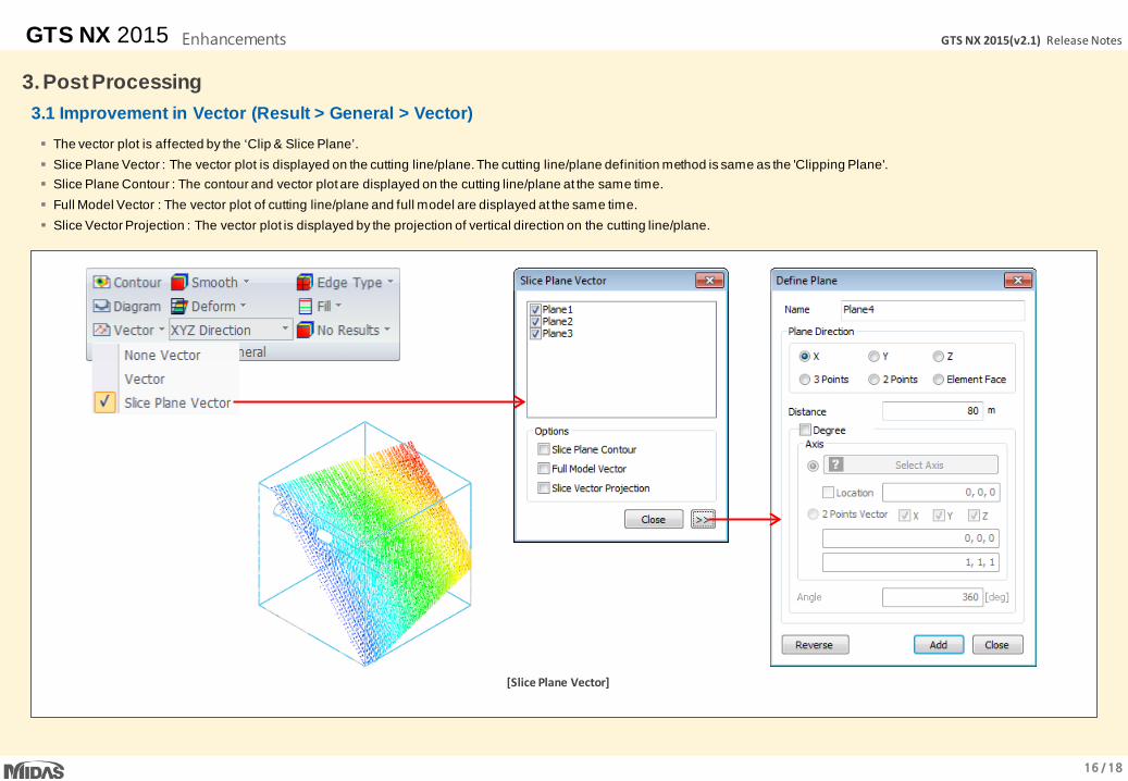
3. Post Processing 3.1 Improvement in Vector (Result > General > Vector) The vector plot is affected by the ‘Clip & Slice Plane’. Slice Plane Vector : The vector plot is displayed on the cutting line/plane. The cutting line/plane definition method is same as the 'Clipping Plane'. Slice Plane Contour : The contour and vector plot are displayed on the cutting line/plane at the same time. Full Model Vector : The vector plot of cutting line/plane and full model are displayed at the same time. Slice Vector Projection : The vector plot is displayed by the projection of vertical direction on the cutting line/plane.

[Slice Plane Vector]

17 / 18


3. Post Processing 3.2 Multi Step Graph (Result > Advanced Function > Others > Multi Step Graph) The results of multi-step are drawn by graph type based on the selected nodes/elements. Analysis set, result type, results, step and nodes/elements will be selected to draw graph. In the ‘Define Graph’, ‘Axis’ is the coordinate of selected nodes/elements, and it is placed at the Y axis of graph. The value of selected nodes/elements is placed at the X axis of graph.

[Result of Multi Step Graph]

18 / 18


3. Post Processing 3.3 Improvement in Flow Quantity (Result > Special Post > Seepage > Flow Quantity) The flow quantity is improved to calculate more easily. The node selection method (Node Mode) and the line/plane definition method (Cutting Mode) are supported. There are ‘Cutting Line’ and ‘Cutting Plane‘ option in the ‘Cutting

Mode’. The ‘Cutting Line’ option calculates flow quantity from nodes within the 'Search Tolerance' by defining ‘2-Points Line’ directly or selecting ‘Edge’. The ‘Cutting Plane‘ option calculates flow quantity from nodes within the 'Search Tolerance' by defining ‘3-Points Plane’ directly or selecting ‘Plane’. The ‘3-Points Plane’ type calculates flow quantity from the infinite plane consisting of three points or the plane only consisting of them with the 'Limited Plane' option.

Once the information for calculating flow quantity is created in the ‘Define Information’ dialogue box, it will be registered in the ‘Define List’. Flow quantity can be calculated by duplicate selecting a number of information registered in the ‘Define List’ and they can be modified or deleted as well. The node information included in the checked ‘Define List’ is displayed in the ‘Node ID’ and duplicated same nodes of a number of information will be treated as one.

[Definition of Flow Quantity]

Release Notes - CSPFea€¦ · The ‘Contraction’ is for the shrinkage in the circumferential...

Documents

Transcript of Release Notes - CSPFea€¦ · The ‘Contraction’ is for the shrinkage in the circumferential...