Relativistic Dynamics

Jason Gross∗

Student at MIT(Dated: October 31, 2011)

I present the energy-momentum-force relations of Newtonian and relativistic dynamics. I inves-tigate the goodness of fit of classical and relativistic models for energy, momentum, and charge-to-mass ratio for electrons traveling at 60%–80% the speed of light. I find that the relativisticmodels do much better than the classical ones (χ2

ν ratios range from about 5 to about about 100).I find the electron charge-to-mass ratio to be (1.54 ± 0.03) · 1011 C/kg, as compared with a bookvalue of 1.758 820 088(39) · 1011 C/kg. I find the charge of the electron to be (1.5 ± 0.1) · 10−19 Cas compared with a book value of 1.602 176 565(35) · 10−19 C. I find the mass of the electronto be variously (9 ± 2) · 10−31 kg and (1.13 ± 0.04) · 10−30 kg, as compared with a book value of9.109 382 91(40) · 10−31 kg.

I. NEWTONIAN AND RELATIVISTICDYNAMICS

Newtonian dynamics begins with the assumption thatspace and time are flat and absolute. Relativistic dy-namics begins with the assumption that space and timeare flat, and that the speed of light is the same in allinertial reference frames. From these assumptions, theMinkowski metric can be derived, as well as length con-traction and time dilation and the relativistic formulae.

See Appendix A for the conventions and symbolic def-initions I use in this paper.

Newtonian and relativistic dynamics are governed bythe following relations, among others:

Newtonian Relativistic~p = m~v ~p = γm~vE = K + U E2 = p2c2 +m2c4

K = p2/2m K = (γ − 1)mc2

K = mc2(√

1 +(pmc

)2 − 1

)

~F = d~p/dt ~F = d~p/dt

Lastly, the electromagnetic force on a charged particle

is ~F = q ~E + q~v × ~B. This formula is valid both forNewtonian dynamics and relativistic dynamics.

We set out to test relativity, and to determine the elec-tron charge and electron mass.

II. METHODOLOGY AND EXPERIMENTALSETUP

We used high-energy electrons to test relativistic dy-namics, using the setup in Figure 1. High-energy elec-trons are emitted from a radiation source and travel ina circular path through the vacuum chamber due to theuniform magnetic field. At the end of a semi-circularpath, electrons are absorbed by a PIN diode which mea-sures their energy.

∗ jgross@mit.edu

Id: 09.relativistic-dynamics.tex,v 1.37 2010/09/27 20:28:43 nickrhj Exp 3

Velocity SelectorPlate Separation = 0.180± 0.003 cm

Length = 10 cm

��B

Preamp Canberra Mo. 2003BT

Digital Voltmeter Fluke 8012A

Velocity Selector HV Supply: 0-5000 V

Canberra Mo. 2003BT

Bias Voltage Supply: 70 V

EG&G Ortec 428

Amplifier Ortec 471

Oscilloscope

Multi-Channel Analyzer

40.6± 0.4 cm

90Sr/90Y Source

Vacuum Chamber∼ 3× 10−8 Torr

PINVS

FIG. 1: Schematic diagram of the electron trajectory in theapparatus, the particle spectrometer and associated circuitry.The velocity selector is labeled VS, and the diode detectorPIN.

pulses in the narrow range of pulse height channels of theMCA corresponding to the energy range of the detectedelectrons, and 3) the median channel of the pulse heightdistribution. Given these data, the dimensions of theapparatus, and the energy calibration of the PIN detectorone can determine the momentum, energy, and velocityof electrons and estimate the values of e/m, m, and e.

4. THEORY OF THE EXPERIMENT

In the region between the source and the velocity se-lector, where only a magnetic field exists, the motion isdescribed by the equation

e|~v|Bc

=

∣∣∣∣d~p

dt

∣∣∣∣ = ω|~p| = |~v|pρ, (10)

so

B =

(c

eρ

)p, (11)

where ρ is the radius of curvature of the particle trajec-tory under the influence of the magnetic force. Placementof the source, the collimator, and the aperture of the ve-locity selector on a circle of radius ρ allows only particleswith a momentum in a narrow range around Beρ/c toenter the velocity selector. In the region between the ve-

locity selector plates ~E, ~B, and ~v are perpendicular toeach other so one can write for particles that experiencezero deflecting force and go exactly parallel to the platesthe relation

eE − evB

c= 0. (12)

The voltage between the velocity selector plates is knownfrom Faraday’s law,

V =

∮~E · d~, (13)

and therefore E = V/d. Hence

β = |~v|/c = E/B. (14)

Thus, for any combination of E and B such that E < B,the velocity selector transmits particles with velocitiesnear E/B in a narrow range of magnitudes whose widthdepends on the geometry of the gap between the plates.

A plot of measured values of B against the ratio E/Breveals the relation between momentum and velocity. Ac-cording to the classical equation (1), the plot would befit by a straight line with a slope of (mc2)/(eρ). Devia-tion from a straight line as E/B → 1 indicates the failureof the classical relation between momentum and velocityas the velocity approaches c. According to the relativityequation (3), a plot of B against (E/B)[1− (E/B)2]−1/2

should be fit by a straight line with a slope of (mc2)/(eρ).From the slope and knowledge of the values of c and ρone can estimate the invariant quantity e/m.

In the experiment it is a good idea to set the magneticfield and then determine the voltage between the selectorplates that gives the highest rate of counts of electronsthat traverse the circular path and pass between the ve-locity selector plates to strike the PIN diode detector.

Note that measurements of E and B alone yield a de-termination of e/m but neither e nor m separately. Thisis characteristic of all experiments involving only electro-magnetic forces. Why is this so? Consider the analogyto the problem of determining the ratio of gravitationalto inertial mass of a body moving under the influenceof gravity. (Incidentally, the Johnson Shot Noise experi-ment in Junior Lab yields the measurement of e.)

The PIN diode detector combines the virtues of anultra-thin entrance window and surface dead layer witha total sensitive thickness sufficient to stop electrons withseveral hundred keV of kinetic energy. Thus, with appro-priate calibration, the PIN diode provides a measure ofthe kinetic energy of the detected electrons. Plots of thekinetic energy against E/B or against [1− (E/B)2]−1/2

reveal the relation between energy and velocity; the slopeof the latter plot yields a value of m (or more conve-niently mc2 expressed in units of keV in terms of whichthe energies of the calibration X and gamma-ray pho-tons are expressed). A plot of energy against B revealsthe deviation of the energy-momentum relation from theclassical quadratic form E = p2/(2m) toward the linearform E = pc valid for a particle moving with a velocityclose to c.

5. APPARATUS DETAILS

The magnet consists of a stack of circular air-core coilsenclosing a spherical volume and connected in series so asto produce a current distribution over the surface of thesphere which is approximately equal to the ideal smoothdistribution required to produce a uniform field insidethe sphere. It turns out that the required distribution of

FIG. 1. Electrons are emitted from the 90Sr/90Y source,travel through the vacuum chamber, enter the velocity selec-tor (VS) and hit the PIN diode, which measures their energy.Figure taken from the lab guide.[1]

A baffle in the middle of the semi-circle selects for elec-trons with a small range of momenta, corresponding tothe small range of radii which pass through a slit in thebaffle.

A capacitive velocity selector further restricts the ve-locities; anything going too slow will be accelerated intoone side of the selector by the electric field, and any-thing going too fast will not be significantly affected bythe electric field, and will hit the other wall due to themagnetic field. At approximately the center of this rangeof momenta, the forces due to the magnetic and electricfields are equal and opposite. It is at this momentum thatthe PIN diode registers a peak in its energy spectrum.

III. EXPERIMENTAL THEORY

We have three relevant parameters for each stream ofelectrons: the energy, from the PIN diode and MCA,the magnetic field strength, and the peak electric fieldstrength (the value of E for which count rate is maxi-mized).

2

Each of these parameters is related to the momentumof the electron.

When the electron feels only a magnetic field, its mo-tion is circular; it’s governed by the equation evB =|d~p/dt| = ωp = vp/ρ which becomes p = eBρ.

The peak in count rate occurs at the momentum atwhich electrons in the velocity selector feel no force:

~F = e ~E + e~v × ~B = 0 (1)

or E = vB. Since E = V/d, we then have

β = v/c = E/(cB) = V/(cBd). (2)

The spread of electron energies about this value is as-sumed to be symmetric, so that we may simply find anapproximate center, which is also the peak value. If thisassumption is inaccurate, the calculations which use en-ergies are slightly more inaccurate than the analysis inthis paper would lead one to believe.

Finally, the measured energy is hypothesized to be re-lated to the momentum of the electron via either the clas-sical formula K = p2/2m or the relativistic formula(s)

K = (γ − 1)mc2 =√p2c2 +m2c4 −mc2. (3)

We may thus determine goodness-of-fit for themomentum-velocity relationships and for the energy-momentum relationships (if we take the textbook valueof me), and we may calculate the ratio e/me under eachregime; classically, we get e/me = V/(B2ρd), and rela-

tivistically, we get e/me = cV/(Bρ√B2c2d2 − V 2). If we

assume the approximate accuracy of relativity (i.e., giveup classical fitting), we may determine the ratio of e/me

by comparing p = eBρ to K = (γ − 1)mc2 and we may

use K =√p2c2 +m2c4 − mc2 to determine me and e

simultaneously.

IV. PROCEDURE

IV.1. Calibration

In order to get a meaningful reading from either theGauss-meter or the MCA, we needed to calibrate theformer to the magnetic field and the latter to a knownenergy spectrum.

The Gauss-meter calibration was mostly straightfor-ward; a description can be found in [1]. We found a vari-ation of approximately 2 G along the track. Estimationof this variation was made less accurate by the fact that

the ~B field tends to decrease over time as the wires heatup, and we only had one Gauss-meter; we were unable tofix B at a point while we measured variation. Repeatedsweeps, however, suggested that 2 G is roughly accurate.

The MCA was calibrated against a 133Ba source. Theenergy spectrum of this source was obtained from [2] and[3]. Compton edges were calculated via the formula

ECompton =2E2

mec2 + 2E(4)

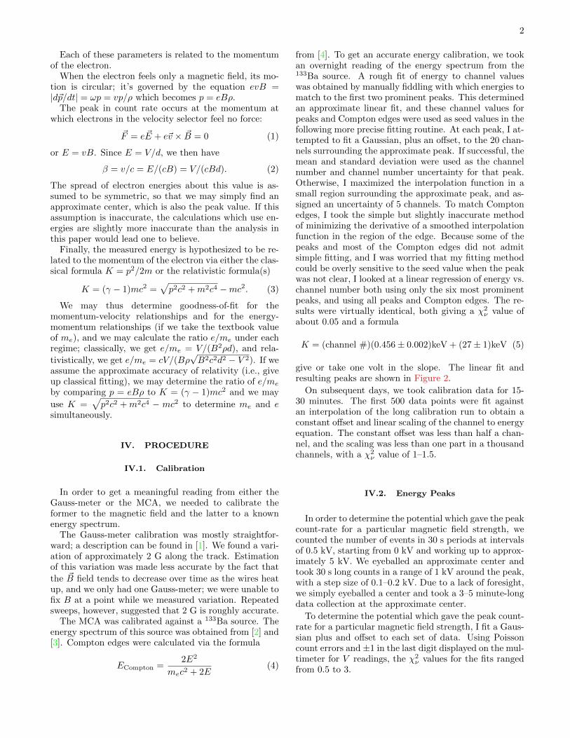
from [4]. To get an accurate energy calibration, we tookan overnight reading of the energy spectrum from the133Ba source. A rough fit of energy to channel valueswas obtained by manually fiddling with which energies tomatch to the first two prominent peaks. This determinedan approximate linear fit, and these channel values forpeaks and Compton edges were used as seed values in thefollowing more precise fitting routine. At each peak, I at-tempted to fit a Gaussian, plus an offset, to the 20 chan-nels surrounding the approximate peak. If successful, themean and standard deviation were used as the channelnumber and channel number uncertainty for that peak.Otherwise, I maximized the interpolation function in asmall region surrounding the approximate peak, and as-signed an uncertainty of 5 channels. To match Comptonedges, I took the simple but slightly inaccurate methodof minimizing the derivative of a smoothed interpolationfunction in the region of the edge. Because some of thepeaks and most of the Compton edges did not admitsimple fitting, and I was worried that my fitting methodcould be overly sensitive to the seed value when the peakwas not clear, I looked at a linear regression of energy vs.channel number both using only the six most prominentpeaks, and using all peaks and Compton edges. The re-sults were virtually identical, both giving a χ2

ν value ofabout 0.05 and a formula

K = (channel #)(0.456± 0.002)keV + (27± 1)keV (5)

give or take one volt in the slope. The linear fit andresulting peaks are shown in Figure 2.

On subsequent days, we took calibration data for 15-30 minutes. The first 500 data points were fit againstan interpolation of the long calibration run to obtain aconstant offset and linear scaling of the channel to energyequation. The constant offset was less than half a chan-nel, and the scaling was less than one part in a thousandchannels, with a χ2

ν value of 1–1.5.

IV.2. Energy Peaks

In order to determine the potential which gave the peakcount-rate for a particular magnetic field strength, wecounted the number of events in 30 s periods at intervalsof 0.5 kV, starting from 0 kV and working up to approx-imately 5 kV. We eyeballed an approximate center andtook 30 s long counts in a range of 1 kV around the peak,with a step size of 0.1–0.2 kV. Due to a lack of foresight,we simply eyeballed a center and took a 3–5 minute-longdata collection at the approximate center.

To determine the potential which gave the peak count-rate for a particular magnetic field strength, I fit a Gaus-sian plus and offset to each set of data. Using Poissoncount errors and±1 in the last digit displayed on the mul-timeter for V readings, the χ2

ν values for the fits rangedfrom 0.5 to 3.

3

Residuals

E

keV� channel H0.456 ± 0.002L + H27. ± 1.L

ΧΝ2

� 0.05

200 400 600 800 1000Channel ð

100

200

300

400

500E HkeVL

31. keV

53.161 keV61.9941 keV

79.6139 keV80.9971 keV

104.094 keV

143.629 keV160.613 keV

164.269 keV

207.269 keV

223.234 keV

230.455 keV

276.398 keV302.853 keV

356.017 keV

383.851 keV

0 200 400 600 800 1000Channel ð

2

4

6

8

10

12

14

logHCountL

FIG. 2. Linear fit to the most prominent energy peaks, alongwith the log-scale spectrum collected overnight with peaksand Compton edges shown and labeled.

V. ANALYSIS AND RESULTS

V.1. Comparing Relativity and Newton

V.1.1. Momentum-Velocity Relationships

Since p = eBρ, Newtonian dynamics predicts thatβ = eBρ/(mec), while relativity predicts that β =√

1− β2eBρ/(mec). Plotting our data and these twocurves gives Figure 4.

Although relativity is clearly much better, there’s asystematic error. I hypothesize that it comes from a con-stant offset in some combination of V , B, d and ρ. Ifit the data to the classical and relativistic curves usingeach of these as fit parameters in succession. For eachparameter except for d, the residuals retained a strongsystematic correlation with B. Using d as a fit parame-ter and assuming the textbook values of e and me givesa χ2

ν value of about 0.05. This suggests that I overesti-mated the error in my values. The most likely candidateis the B field, for which I used an uncertainty of 2 G;we measured 2 G variation along the path, but fixed theB field at a point to within 0.02 G. Using 0.02 G as theuncertainty in B gives a much more reasonable χ2

ν of 0.5,and a value of d = 0.1696(4) cm (as compared with thevalue of d = 0.180(3) cm given in [1]).

Classical

Relativistic

ΧΝ2

Classical � 2.´102

ΧΝ2

Relativistic � 4.

70 80 90 100 110 120B HGaussL0.4

0.6

0.8

1.0

1.2

1.4Β

FIG. 3. Plot of β vs. B, classical and relativistic predic-tions, assuming textbook values of electron charge and mass.Dotted lines show uncertainty in β due to uncertainty in ρ.

Residuals

70 80 90 100 110 120B HGaussL0.4

0.6

0.8

1.0

1.2

1.4Β

Relativistic; Fitting Dd

FIG. 4. Plot of β vs. B, using d as a fit parameter. χ2ν = 0.05

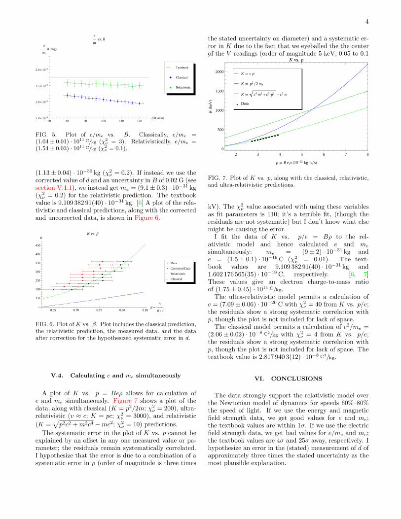
V.2. Calculating e/me

Instead of comparing the plot of β vs. B to the pre-dictions of relativity, we may instead calculate e/me =βc/(Bρ) and fit this to a constant. The plot of e/me

vs. B is shown in Figure 5. The classical value ise/me = (1.04± 0.01) · 1011 C/kg with χ2

ν = 3. The rel-ativistic value is e/me = (1.54± 0.03) · 1011 C/kg withχ2ν = 0.1. If we instead use the revised uncer-

tainty of ±0.02 G in B we get the classical value of(1.053± 0.008) · 1011 C/kg (χ2

ν = 10) and the relativisticvalue of (1.54± 0.02) · 1011 C/kg (χ2

ν = 0.3). The text-book value is 1.758 820 088(39) · 1011 C/kg. [5]

V.3. Calculating me; K vs. β

We may calculate β = V/(Bcd). Relativity pre-dicts that K = ((1 − β2)−1/2 − 1)mec

2. Newtonianmechanics predicts that K = 1

2mec2β2. A fit to the

classical equation gives me = (1.95± 0.02) · 10−32 kg(χ2ν = 3) A fit to the relativistic equation gives me =

4

70 80 90 100 110 120B HGaussL5.0 ´ 1010

1.0 ´ 1011

1.5 ´ 1011

2.0 ´ 1011

e

me

HC � kgL

e

mvs. B

Relativistic

Classical

Textbook

FIG. 5. Plot of e/me vs. B. Classically, e/me =(1.04 ± 0.01) · 1011 C/kg (χ2

ν = 3). Relativistically, e/me =(1.54 ± 0.03) · 1011 C/kg (χ2

ν = 0.1).

(1.13± 0.04) · 10−30 kg (χ2ν = 0.2). If instead we use the

corrected value of d and an uncertainty inB of 0.02 G (seesection V.1.1), we instead get me = (9.1± 0.3) · 10−31 kg(χ2ν = 0.2) for the relativistic prediction. The textbook

value is 9.109 382 91(40) · 10−31 kg. [6] A plot of the rela-tivistic and classical predictions, along with the correctedand uncorrected data, is shown in Figure 6.

0.65 0.70 0.75 0.80 0.85Β �

V

B c d

150

200

250

300

350

400

450

KK vs. Β

Classical

Relativistic

Corrected Data

Data

FIG. 6. Plot of K vs. β. Plot includes the classical prediction,the relativistic prediction, the measured data, and the dataafter correction for the hypothesized systematic error in d.

V.4. Calculating e and me simultaneously

A plot of K vs. p = Beρ allows for calculation ofe and me simultaneously. Figure 7 shows a plot of thedata, along with classical (K = p2/2m; χ2

ν = 200), ultra-relativistic (v ≈ c; K = pc; χ2

ν = 3000), and relativistic

(K =√p2c2 +m2c4 −mc2; χ2

ν = 10) predictions.

The systematic error in the plot of K vs. p cannot beexplained by an offset in any one measured value or pa-rameter; the residuals remain systematically correlated.I hypothesize that the error is due to a combination of asystematic error in ρ (order of magnitude is three times

the stated uncertainty on diameter) and a systematic er-ror in K due to the fact that we eyeballed the the centerof the V readings (order of magnitude 5 keV; 0.05 to 0.1

Data

K � c4 m2 + c2 p2 - c2 m

K � p2 � 2 me

K � c p

2 3 4 5 6 7 80

500

1000

1500

2000

p � B e Ρ H10-22 kg m � sL

KHke

VL

K vs. p

FIG. 7. Plot of K vs. p, along with the classical, relativistic,and ultra-relativistic predictions.

kV). The χ2ν value associated with using these variables

as fit parameters is 110; it’s a terrible fit, (though theresiduals are not systematic) but I don’t know what elsemight be causing the error.

I fit the data of K vs. p/e = Bρ to the rel-ativistic model and hence calculated e and me

simultaneously: me = (9± 2) · 10−31 kg ande = (1.5± 0.1) · 10−19 C (χ2

ν = 0.01). The text-book values are 9.109 382 91(40) · 10−31 kg and1.602 176 565(35) · 10−19 C, respectively. [6, 7]These values give an electron charge-to-mass ratioof (1.75± 0.45) · 1011 C/kg.

The ultra-relativistic model permits a calculation ofe = (7.09± 0.06) · 10−20 C with χ2

ν = 40 from K vs. p/e;the residuals show a strong systematic correlation withp, though the plot is not included for lack of space.

The classical model permits a calculation of e2/me =(2.06± 0.02) · 10−8 C2/kg with χ2

ν = 4 from K vs. p/e;the residuals show a strong systematic correlation withp, though the plot is not included for lack of space. Thetextbook value is 2.817 940 3(12) · 10−8 C2/kg.

VI. CONCLUSIONS

The data strongly support the relativistic model overthe Newtonian model of dynamics for speeds 60%–80%the speed of light. If we use the energy and magneticfield strength data, we get good values for e and me;the textbook values are within 1σ. If we use the electricfield strength data, we get bad values for e/me and me;the textbook values are 4σ and 25σ away, respectively. Ihypothesize an error in the (stated) measurement of d ofapproximately three times the stated uncertainty as themost plausible explanation.

5

[1] N. R. Hunter-Jones, “Relativistic dynamics,” (2010).[2] T. Pantazis, “Scintillation detector and multichannel an-

alyzer (mca) (homeland security applications),” (2006).[3] R. B. Firestone and L. P. Ekstrom, “Table of isotopes

decay data,” (1999).[4] “Compton edge,” (2011).[5] “CODATA value: electron charge to mass quotient,”

(2010).[6] “CODATA value: electron mass,” (2010).[7] “CODATA value: electron charge,” (2010).

ACKNOWLEDGMENTS

The author gratefully acknowledges his lab partnerThomas Vandermeulen for help collecting the data, andthe J-Lab staff for their help in experimentation. Thanksespecially to Professor Nergis Mavalvala for suggestingthat I use d as a fit parameter.

Appendix A: Notational Conventions

Throughout this paper, ~a denotes a polar vector withunsigned magnitude a pointing in the direction of theunit vector a. I use SI units and equations, and thefollowing variables:m is rest mass; me is the mass of an electronq is signed charge; −e is the charge of an electron~p is momentum~F is force~v is velocity~E is the electric field~B is the magnetic fieldV is an electric potentialc is the speed of lightE is total energy; K is kinetic energy~β = ~v/c

γ = 1/√

1− β2 is the Lorentz factort is timeρ is a radius of circular motiond is a separation between plates of a capacitor~ω is angular velocity