![Relativistic Brownian Motion and Diffusion Processes · 2016-05-18 · Lebenslauf 151 Danksagung 152. Symbols M rest mass of the Brownian particle ... Wheeler and Feynman [222,223],](https://static.fdocuments.net/doc/165x107/5f32bf03cc60a53c240c2db2/relativistic-brownian-motion-and-diiusion-processes-2016-05-18-lebenslauf-151.jpg)
Relativistic Brownian Motion and Diffusion Processes · Relativistic Brownian Motion and...
155
Relativistic Brownian Motion and Diffusion Processes Dissertation Institut f¨ ur Physik Mathematisch-Naturwissenschaftliche Fakult¨at Universit¨atAugsburg eingereicht von J¨ornDunkel Augsburg, Mai 2008
Transcript of Relativistic Brownian Motion and Diffusion Processes · Relativistic Brownian Motion and...
Relativistic Brownian Motion and Diffusion Processes
Dissertation
Institut fur Physik
Mathematisch-Naturwissenschaftliche Fakultat
Universitat Augsburg
eingereicht von
Jorn Dunkel
Augsburg, Mai 2008

Erster Gutachter: Prof. Dr. Peter Hanggi
Zweiter Gutachter: Prof. Dr. Thilo Kopp
Dritter Gutachter: Prof. Dr. Werner Ebeling
Tag der mundlichen Prufung: 22.07.2008
Contents
Symbols 3
1 Introduction and historical overview 5
2 Nonrelativistic Brownian motion 13
2.1 Langevin and Fokker-Planck equations . . . . . . . . . . . . . . . . . . . . 14
2.1.1 Linear Brownian motion: Ornstein-Uhlenbeck process . . . . . . . . 14
2.1.2 Nonlinear Langevin equations . . . . . . . . . . . . . . . . . . . . . 19
2.1.3 Other generalizations . . . . . . . . . . . . . . . . . . . . . . . . . . 22
2.2 Microscopic models . . . . . . . . . . . . . . . . . . . . . . . . . . . . . . . 22
2.2.1 Harmonic oscillator model . . . . . . . . . . . . . . . . . . . . . . . 23
2.2.2 Elastic binary collision model . . . . . . . . . . . . . . . . . . . . . 26
3 Relativistic equilibrium thermostatistics 35
3.1 Preliminaries . . . . . . . . . . . . . . . . . . . . . . . . . . . . . . . . . . 36
3.1.1 Notation and conventions . . . . . . . . . . . . . . . . . . . . . . . 36
3.1.2 Probability densities in special relativity . . . . . . . . . . . . . . . 37
3.2 Thermostatistics of a relativistic gas . . . . . . . . . . . . . . . . . . . . . 40
3.2.1 Relative entropy, Haar measures and canonical velocity distributions 40
3.2.2 Relativistic molecular dynamics simulations . . . . . . . . . . . . . 45
4 Relativistic Brownian motion 53
4.1 Langevin and Fokker-Planck equations . . . . . . . . . . . . . . . . . . . . 54
4.1.1 Construction principle and conceptual aspects . . . . . . . . . . . . 55
4.1.2 Examples . . . . . . . . . . . . . . . . . . . . . . . . . . . . . . . . 59
4.1.3 Asymptotic mean square displacement . . . . . . . . . . . . . . . . 61
4.2 Moving observer . . . . . . . . . . . . . . . . . . . . . . . . . . . . . . . . . 66
4.2.1 Fokker-Planck and Langevin equations . . . . . . . . . . . . . . . . 67
4.2.2 Covariant formulation . . . . . . . . . . . . . . . . . . . . . . . . . 68
4.3 Relativistic binary collision model . . . . . . . . . . . . . . . . . . . . . . . 69
1
2 CONTENTS
5 Non-Markovian relativistic diffusion 75
5.1 Reminder: nonrelativistic diffusion equation . . . . . . . . . . . . . . . . . 76
5.2 Telegraph equation . . . . . . . . . . . . . . . . . . . . . . . . . . . . . . . 78
5.3 Relativistic diffusion propagator . . . . . . . . . . . . . . . . . . . . . . . . 82
6 Summary and outlook 87
Appendices
A Special relativity (basics) 93
A.1 Notation and definitions . . . . . . . . . . . . . . . . . . . . . . . . . . . . 93
A.2 Lorentz-Poincare transformations . . . . . . . . . . . . . . . . . . . . . . . 95
B Normalization constants 99
B.1 Juttner function . . . . . . . . . . . . . . . . . . . . . . . . . . . . . . . . . 99
B.2 Diffusion propagator . . . . . . . . . . . . . . . . . . . . . . . . . . . . . . 100
C Stochastic integrals and calculus 101
C.1 Ito integral . . . . . . . . . . . . . . . . . . . . . . . . . . . . . . . . . . . 102
C.1.1 One-dimensional case . . . . . . . . . . . . . . . . . . . . . . . . . . 102
C.1.2 The n-dimensional case . . . . . . . . . . . . . . . . . . . . . . . . . 103
C.2 Stratonovich-Fisk integral . . . . . . . . . . . . . . . . . . . . . . . . . . . 104
C.2.1 One-dimensional case . . . . . . . . . . . . . . . . . . . . . . . . . . 104
C.2.2 The n-dimensional case . . . . . . . . . . . . . . . . . . . . . . . . . 105
C.3 Backward Ito integral . . . . . . . . . . . . . . . . . . . . . . . . . . . . . . 106
C.3.1 One-dimensional case . . . . . . . . . . . . . . . . . . . . . . . . . . 106
C.3.2 The n-dimensional case . . . . . . . . . . . . . . . . . . . . . . . . . 107
C.4 Comparison of stochastic integrals . . . . . . . . . . . . . . . . . . . . . . . 107
C.5 Numerical integration . . . . . . . . . . . . . . . . . . . . . . . . . . . . . . 110
D Higher space dimensions 111
D.1 Lab frame . . . . . . . . . . . . . . . . . . . . . . . . . . . . . . . . . . . . 111
D.2 Moving observer . . . . . . . . . . . . . . . . . . . . . . . . . . . . . . . . . 113
Bibliography 115
Lebenslauf 151
Danksagung 152
Symbols
M rest mass of the Brownian particle
m rest mass of a heat bath particle
Σ inertial laboratory frame := rest frame of the heat bath
Σ′; Σ∗ moving frame; comoving rest frame of the Brownian particle
O; O′ lab observer; moving observer
t time coordinate
τ proper time of the Brownian particle
c vacuum speed of light (set to unity throughout, i.e., c = 1)
d number of space dimensions
X,x position coordinate
V ,v particle velocity
w observer velocity
P ,p momentum coordinates
E, ǫ particle energy
η = (ηαβ) Minkowski metric tensor
Λ Lorentz transformation (matrix)
γ Lorentz factor. γ(v) = (1 − v2)−1/2
Xα (contravariant) time-space four-vector (Xα) = (t,X), α = 0, 1, . . . , d
P α energy-momentum four-vector, (P α) = (E,P )
Uα velocity four-vector, Uα = P α/M
f one-particle phase space probability density
one-particle position probability density
φ one-particle momentum probability density
ψ one-particle velocity probability density
kB Boltzmann constant (set to unity throughout, i.e., kB = 1)
T temperature
β inverse thermal energy β := (kBT)−1
S relative entropy
α friction coefficient
3
4 CONTENTS
D noise amplitude
D spatial diffusion constant
B(s) d-dimensional standard Wiener process with time parameter s
P probability measure of the Wiener process
∗ Ito (pre-point) interpretation of the stochastic integral
◦ Stratonovich-Fisk (mid-point) interpretation of the stochastic integral
• backward Ito (post point) interpretation of the stochastic integral
N set of natural numbers 1, 2, . . .
Z set of integer numbers
R set of real numbers
λ Lebesgue measure
µ, ρ measures
〈X〉 expected value of a random variable X
Chapter 1
Introduction and historical overview
In his annus mirabilis 1905 Albert Einstein published four manuscripts [1–4] that would
forever change the world of physics. Two of those papers [2, 3] laid the foundations for
the special theory of relativity, while another one [4] solved the longstanding problem of
classical (nonrelativistic) Brownian motion.1 Barring gravitational effects [5, 6], special
relativity has proven to be the correct framework for describing physical processes on
all terrestrial scales [7, 8]. Accordingly, during the past century extensive efforts have
been made to adapt established nonrelativistic theories such as, e.g., thermodynamics,
quantum mechanics or field theories [9] to the requirements of special relativity. Following
this tradition, the present thesis investigates how stochastic concepts such as Brownian
motion may be generalized within the framework of special relativity. The subsequent
chapters intend to provide a cohesive summary of results obtained during the past three
years [10–17], also taking into account important recent contributions by other authors (see,
e.g., [18–24]).
Historically, the term ‘Brownian motion’ refers to the irregular dynamics exhibited by
a test particle (e.g., dust or pollen) in a liquid environment. This phenomenon, already
mentioned by Ingen-Housz [25, 26] in 1784, was first analyzed in detail by the Scottish
botanist Robert Brown [27] in 1827. About 80 years later, Einstein [4], Sutherland [28]
and von Smoluchowski [29] were able to theoretically explain these observations. They
proposed that Brownian motion is caused by quasi-random, microscopic interactions with
molecules forming the liquid. In 1909 their theory was confirmed experimentally by Per-
rin [30], providing additional evidence for the atomistic structure of matter. During the
first half of the 20th century the probabilistic description of Brownian motion processes
was further elaborated in seminal papers by Langevin [31, 32], Fokker [33], Planck [34],
Klein [35], Uhlenbeck and Ornstein [36] and Kramers [37]. Excellent reviews of these early
contributions are given by Chandrasekhar [38] and Wang and Uhlenbeck [39].
1Einstein’s first paper [1] provided the theoretical explanation for the photoelectric effect.
5
6 CHAPTER 1. INTRODUCTION AND HISTORICAL OVERVIEW
In parallel with the studies in the field of physics, outstanding mathematicians like Bache-
lier [40], Wiener [41–43], Kolmogoroff [44–46], Feller [47], and Levy [48, 49] provided a
rigorous basis for the theory of Brownian motions and stochastic processes in general.
Between 1944 and 1968 their groundbreaking work was complemented by Ito [50,51], Gih-
man [52–54], Fisk [55,56] and Stratonovich [57–59], who introduced and characterized dif-
ferent types of stochastic integrals or, equivalently, stochastic differential equations (SDEs).
The theoretical analysis of random processes was further developed over the past decades,
and the most essential results are discussed in several excellent textbook references [60–66]2.
The modern theory of stochastic processes goes far beyond the original problem considered
by Einstein and his contemporaries, and the applications cover a wide range of different
areas including physics [67–74], biology [75, 76], economy and finance [77–79].
The present thesis is dedicated to the question how SDE-based Brownian motion models
can be generalized within the framework of special relativity. In the physics literature [65],
SDEs are often referred to as Langevin equations [31, 32], and we shall use both terms
synonymously here. From a mathematical point of view, SDEs [64] determine well-defined
models of stochastic processes; from a physicist’s point of view, their usefulness for the
description of a real system is a priori an open issue. Therefore, the derivation of nonrel-
ativistic Langevin equations from microscopic models has attracted considerable interest
over the past 60 years [13,80–86]. Efforts in this direction helped to clarify the applicability
of SDEs to physical problems and led, among others, to the concept of quantum Brownian
motion [82, 87–99].3
If one aims at generalizing the classical Brownian motion concepts to special relativity,
then several elements from relativistic equilibrium thermodynamics and relativistic statis-
tical mechanics play an important role. The first papers on relativistic thermodynamics
were written by Einstein [109] and Planck [110, 111] in 1907. A main objective of their
studies was to clarify the Lorentz transformation laws of thermodynamic variables (tem-
perature, pressure, etc.).4 In 1963 the results of Einstein and Planck were questioned by
Ott [115], whose work initiated an intense debate about the correct relativistic transfor-
mation behavior of thermodynamic quantities [116–160].5 However, as clarified by van
Kampen [137] and Yuen [161], the controversy surrounding relativistic thermodynamics
can be resolved by realizing that thermodynamic quantities can be defined in different,
2The history of the mathematical literature on Brownian motions and stochastic processes is discussed
extensively in Section 2.11 of Ref. [64]; see also Chapters 2-4 in Nelson [61].3The vast literature on classical Brownian motion processes and their various applications in nonrel-
ativistic physics is discussed in several survey articles [68–73, 100–104]. Nonrelativistic generalizations of
the standard theory as, e.g., anomalous diffusion processes have been summarized in [73, 105, 106], while
review articles on nonrelativistic quantum Brownian motion can be found in [97, 98, 107,108].4See also Pauli [112], Tolman [113] and van Dantzig [114] for early discussions of this problem.5The pre-1970 literature on this disputed issue has been reviewed by Yuen [161] and Ter Haar and
Wegland [162]; more recent surveys can be found in [163–165].

7
equally consistent ways.
While some authors considered relativistic thermodynamics as a purely macroscopic the-
ory, others tried to adopt a more fundamental approach by focussing on relativistic equi-
librium statistical mechanics. Pioneering work in the latter direction is due to von Mosen-
geil [166], who studied the radiation of a moving cavity, and Juttner [167], who derived in
1911 the relativistic generalization of Maxwell’s velocity distribution [168].6 Two decades
later, in 1928, Juttner [170] also calculated the equilibrium distributions for ideal relativis-
tic quantum gases. Relativistic generalizations of equipartition and virial theorems [171]
were discussed by Pauli [112] in 1921 and Einbinder [172] in 1948.7 Research on rela-
tivistic equilibrium thermostatistics experienced its most intense phase between 1950 and
1970 [124, 125, 133, 137, 146, 176–191]. An excellent exposition on the conceptual founda-
tions and difficulties of relativistic statistical mechanics was given by Hakim [192–194] in
1967. During the past years the field has continued to attract interest [14,17,173,195–219].8
The recurring debate on relativistic thermostatistics can be traced back to the diffi-
culty of treating many-particle interactions in a relativistically consistent manner. In
nonrelativistic physics interactions may propagate at infinite speed, i.e., they can be mod-
elled via instantaneous interaction potentials which enter additively in the Hamilton func-
tion; from that point on, nonrelativistic statistical mechanics emerges without much dif-
ficulty [220, 221]. Unfortunately, the situation becomes significantly more complicated in
the relativistic case: Due to their finite propagation speed, relativistic interactions should
be modelled by means of fields that can exchange energy with the particles [6]. These fields
add an infinite number of degrees of freedom to the particle system. Elimination of the
field variables from the dynamical equations may be possible in some cases but this proce-
dure typically leads to retardation effects, i.e., the particles’ equations of motions become
non-local in time [192, 193, 222–225]. Thus, in special relativity it is usually very difficult
or even impossible9 to develop a consistent field-free Hamilton formalism for interacting
many-particle systems [225–228].
Seminal contributions to the theory of relativistic many-particle interactions were pro-
vided by Fokker [229], Wheeler and Feynman [222, 223], Pryce [230], Havas and Gold-
berg [231, 232], and Van Dam and Wigner [224, 225]. Over the past decades several no-
interaction theorems were proven [225–228] that, within their respective qualifications,
forbid certain types of interaction models within the framework of special relativity. The
mathematical structure of relativistic many-particle interactions was analyzed in detail by
6See also Synge’s textbook classic [169].7More recent investigations related to these specific topics can be found in [173–175].8In particular, some recent papers [14, 206,209,211,215–217] have raised doubts about the correctness
of Juttner’s equilibrium distribution [167, 170], but relativistic molecular dynamics simulations confirm
Juttner’s prediction [17, 214]; cf. Section 3.2 below.9An exception is the one-dimensional gas of point particles with strictly localized elastic interactions
(cf. discussion in Chapter 3 below).
8 CHAPTER 1. INTRODUCTION AND HISTORICAL OVERVIEW
Arens and Babbitt [233], and various semi-relativistic approximations have been discussed,
e.g., in [234–236].10 Another, intensely studied method for describing relativistic interac-
tions is based on the so-called constraint formalism [200, 211, 248–264]. The foundations
of this approach were worked out by Dirac [248] in 1949, who aimed at constructing a
consistent relativistic quantum theory. However, compared with the nonrelativistic case,
it seems fair to say that neither of the various formulations has led to a relativistic statis-
tical many-particle theory that is on the same rigorous, commonly accepted footing as its
nonrelativistic counterpart.11
In spite of the difficulties impeding a rigorous treatment of relativistic many-particle sys-
tems, considerable progress has been made over the past century in constructing an approx-
imate relativistic kinetic theory based on one-particle phase space probability density func-
tions (PDFs). Early pioneering work that paved the way for the relativistic generalization
of the nonrelativistic Boltzmann equation [267,268] was done by Eckart [269], Lichnerowicz
and Marrot [270], Kluitenberg et al. [271], Beliaev and Budker [272], Synge [169], and Is-
rael [273].12 Comprehensive introductions to relativistic kinetic theory can be found in the
textbooks by Stewart [288], de Groot et al. [289], and Cercignani and Kremer [290], or also
in the reviews by Ehlers [291] and Andreasson [292].13
From relativistic kinetic theory [289,290] it is only a relatively small step to formulating
a theory of relativistic Brownian motion processes in terms of Fokker-Planck equations
(FPEs) and Langevin equations. While the relativistic Boltzmann equation is a nonlinear
partial integro-differential equation, FPEs are linear partial differential equations and,
therefore, can be solved more easily [63]. In this work, we will mostly focus on relativistic
stochastic processes that are characterized by linear evolution equations for their respective
one-particle (transition) PDFs. The research in this direction may be roughly divided into
four different areas, although, of course, there are substantial overlaps and intersections
between them:
a) Relativistic Fokker-Planck equations in phase space. Similar to the relativistic Boltz-
mann equation, relativistic FPEs can be used to model non-equilibrium and relax-
ation phenomena in relativistic many-particle systems. Generally, an FPE can be
derived from a Langevin equation or as an approximation to a more general linear
master equation governing the stochastic process [65, 293]. Yet another way of de-
10Kerner [237] has edited a reprint collection covering large parts of the pre-1972 literature on relativistic
action-at-a-distance models, and more recent contributions can be found in [199,200,238–247].11For a more detailed discussion of relativistic many-particle theory, we refer to the insightful consider-
ations in the orginal papers of Van Dam and Wigner [224,225] and Hakim [192–194,265] as well as to the
recent review by Hakim and Sivak [266].12See also [138,153,196,234,274–287].13Although standard relativistic kinetic theory can be considered as well-established nowadays [289,290],
some authors questioned its validity in recent years and proposed modifications of the relativistic Boltz-
mann equation [206,215–217]. Recent numerical simulations [17,214] support the standard theory [289,290].
9
riving an FPE is to approximate the collision integrals in the nonlinear Boltzmann
equation by a differential expression that contains effective friction and diffusion coef-
ficients [278,294]. The latter approach has been applied successfully in different areas
of physics over the past decades, including plasma physics [278, 295–307], high en-
ergy physics [308–314], and astrophysics [315–320]. For example, in 1970 Akama [278]
started from the relativistic Boltzmann equation to construct the FPE for a relativis-
tic plasma. In the 1980/1990s this approach was further elaborated [295–303] and
several numerical methods for solving FPEs were developed [298, 321–323]. During
the past three decades stochastic concepts assumed an increasing importance in other
areas of high energy physics as well. In the early 1980s relativistic Fokker-Planck-
type equations played an important role in the debate about whether or not the
black body radiation spectrum is compatible with Juttner’s relativistic equilibrium
distribution [173,324–327]. More recently, FPEs have also been used to model diffu-
sion and thermalization processes in quark-gluon plasmas, as produced in relativistic
heavy ion collision experiments [308–310, 312–314]. Similarly, the combination of
probabilistic and relativistic concepts can be useful to describe complex high energy
processes in astrophysics [315–320,328].
b) Relativistic Langevin equations. A complementary approach towards relativistic sto-
chastic processes is based on relativistic Langevin equations [10,11,13,18–22,329–335].
The latter yield explicit sample trajectories for the stochastic motion of a relativistic
Brownian particle. They are, therefore, particularly useful for numerical simulations.
Relativistic Langevin equations may either be postulated as phenomenological model
equations [10,18] or derived from more precise microscopic models by imposing a se-
quence of approximations [13]. Compared with the nonrelativistic case, the latter
task becomes considerably more complicated due to the aforementioned difficulties
in classical relativistic many-particle theory. The phenomenological Langevin ap-
proach to relativistic Brownian motion was developed by Debbasch et al. [18], who in
1997 proposed a simple relativistic generalization of the classical Ornstein-Uhlenbeck
process [36], called ROUP. As will be discussed in Chapter 4, the ROUP may be con-
sidered as a special limit cases of a larger class of relativistic Langevin processes [12].
Furthermore, complementing the phenomenological Langevin theory of relativistic
Brownian motions, we will analyze the assumptions and approximations that must
be made in order to obtain a relativistic Langevin equations from a 1D microscopic
binary collision model. From a practical point of view, relativistic Langevin equations
provide a useful tool for modelling the dynamics of relativistic particles in a random
environment, since these SDEs may be simulated by using well-established Monte-
Carlo techniques that are numerically robust and efficient [66,79,336]. Very recently,
relativistic Langevin equations have been employed by van Hees et al. [312,313] and
10 CHAPTER 1. INTRODUCTION AND HISTORICAL OVERVIEW
Rapp et al. [314, 337], who analyzed thermalization effects in quark-gluon plasmas,
and also by Dieckmann et al. [338], who studied the thermalization in ultrarelativistic
plasma beam collisions as common in astrophysical settings.
c) Mathematically oriented research. To our knowledge, the first detailed mathe-
matical studies on relativistic diffusion processes were performed independently by
Lopuszanski [339] in 1953, Rudberg [340] in 1957, and Schay [293] in 1961. The work
of these authors was further elaborated by Dudley who published between 1965 and
1974 a series of papers [341–344] that aimed at providing an axiomatic approach to
Lorentz invariant Markov processes in phase space. Independently, a similar pro-
gram was pursued by Hakim [192–194,345,346] between 1965 and 1968. Hakim not
only derived different forms of relativistic FPEs [345,346], his insightful analysis also
elucidated the conceptual subtleties of relativistic stochastic processes [346] and rel-
ativistic statistical mechanics [192, 193, 265]. Dudley (Theorem 11.3 in [341]) and
Hakim (Proposition 2 in [346]) proved the non-existence of nontrivial14 Lorentz in-
variant Markov processes in Minkowski space, as already suggested in Lopuszanski’s
early work [339]. This important result implies that it is nontrivial to find acceptable
relativistic generalizations of the well-known nonrelativistic diffusion equation [220]
∂
∂t(t, x) = D∇2(t, x). (1.1)
Put differently, if one wishes to model relativistic random motions by means of a
Markov process [64] with respect to coordinate time t then phase space coordi-
nates have to be used (i.e., position and momentum). The mathematical interest
in relativistic diffusion processes increased in the 1980s and 1990s, when several
authors considered the possibility of extending Nelson’s stochastic quantization ap-
proach [347] to the framework of special relativity, see e.g. [348–369] and also Section
III.H in [370].15 Important recent results on classical relativistic diffusions are due to
Angst and Franchi [23], who were able to characterize the asymptotic behavior of a
large class of special relativistic Brownian motion processes on phase space by means
of a Central Limit Theorem.16
14A diffusion process is considered as ‘nontrivial’ if a typical path has a non-constant, non-vanishing
velocity.15These studies, although interesting from a mathematical point of view, appear to have little physical
relevance because Nelson’s stochastic dynamics [347] fails to reproduce the correct quantum correlation
functions even in the nonrelativistic case [371]. Therefore, the present work focusses primarily on relativistic
non-quantum diffusion processes.16In this context, we also mention the recent work by Rapoport [372,373] and Franchi and Le Jan [374],
who extended the approach of Dudley [341–344] to the framework of general relativity.
11
d) Non-Markovian generalizations of the nonrelativistic diffusion equation (1.1). A
commonly considered ‘relativistic’ generalization of Eq. (1.1) is the telegraph equa-
tion [375–377]
τv∂2
∂t2(t, x) +
∂
∂t(t, x) = D∇2(t, x), (1.2)
with τv > 0 denoting a finite relaxation time scale. Unlike the classical diffusion equa-
tion (1.1), which is recovered for τv = 0, the telegraph equation (1.2) contains a second
order time-derivative and, therefore, describes a non-Markovian process. While the
classical diffusion equation (1.1) permits superluminal propagation speeds, the dif-
fusion fronts described by Eq. (1.2) travel at finite absolute velocity v = (D/τv)1/2.
Masoliver and Weiss [377] discuss four possibilities of deriving Eq. (1.2) from different
underlying models. The first probabilistic derivation of Eq. (1.2) for the 1D case was
given by Goldstein [375] in 1950. His approach was based on a so-called persistent
random walk model originally introduced by Furth [378,379] in 1917 as a paradigm
for diffusive motion in biological systems and later also considered by Taylor [380]
in an attempt to treat turbulent diffusion.17 In contrast to standard non-directed
random walk models, which lead to the classical diffusion equation (1.1) when per-
forming an appropriate continuum limit [64], the random jumps of a persistent walk
take into account the history of a path by assigning a larger probability to those
jumps that point in the direction of the motion before the jump [375,376]. Persistent
random walk models can be used to describe the transmission of light in multiple
scattering media [383] such as foams [384–386] and thin slabs [382, 387]. Similarly,
the telegraph equation (1.2) has been applied in various areas of physics over the past
decades, e.g., to model the propagation of electric signals and heat waves.18 An in-
teresting connection between the free particle Dirac equation [397] and the telegraph
equation (1.2) was pointed out by Gaveau et al. [398] in 1984: The solutions of both
equations may be linked by means of an analytic continuation quite similar to the
relation between the diffusion equation (1.1) and the free particle Schrodinger equa-
tion in the nonrelativistic case.19 On the other hand, the telegraph equation (1.2)
is not the only possible generalization of Eq. (1.1) and a rather critical discussion of
Eq. (1.2) in the context of relativistic heat transport was given by van Kampen [140]
in 1970. In Chapter 5 we will take a closer look at the properties of Eq. (1.2) and
address potential alternatives [15, 405].
17See also Kac [376] and Boguna et al. [381, 382].18A detailed review of the pre-1990 research on heat waves was provided by Joseph and Preziosi [388,389],
while more recent discussions and applications of Eq. (1.2) can be found in [377,390–396].19For further reading about path integral representations of the Dirac propagator we refer to the papers of
Ichinose [399,400], Jacobson and Schulman [401], Barut and Duru [402], and Gaveau and Schulman [403];
see also footnote 7 in Gaveau et al. [398] and problem 2-6, pp. 34-36 in Feynman and Hibbs [404].
12 CHAPTER 1. INTRODUCTION AND HISTORICAL OVERVIEW
Concluding this brief historical overview, we may summarize that the theory of relativistic
Brownian motion and diffusion processes has experienced considerable progress during the
past decade, with applications in various areas of high energy physics [308, 310–312, 314,
393, 394, 406] and astrophysics [318, 320, 328, 338]. From a general perspective, relativis-
tic stochastic processes provide a useful approach whenever one has to model the quasi-
random behavior of relativistic particles in a complex environment. Therefore, it may be
expected that relativistic Brownian motion and diffusion concepts will play an increasingly
important role in future investigations of, e.g., thermalization and relaxation processes in
astrophysics or high energy collision experiments. The present work aims to provide a
comprehensive overview of the theory of relativistic Brownian motions with a particular
emphasis on relativistic Langevin equations. For this purpose, the subsequent parts are
organized as follows. Chapter 2 summarizes the Langevin theory of nonrelativistic Brown-
ian motions in phase space. Chapter 3 discusses relevant aspects of relativistic equilibrium
thermostatistics. Relativistic Langevin equations and their associated FPEs, are consid-
ered in Chapter 4. Chapter 5 is dedicated to relativistic diffusion processes in Minkowski
space-time; as outlined above, such processes must necessarily be non-Markovian. The
thesis concludes with a summary of open questions in Chapter 6, which may serve as a
starting point for future investigations and extensions of the theory. In order to present
the most important ideas and concepts in a transparent way, the discussion in the main
text will focus mostly on the simplest case of one space dimension (1D). The generalization
to higher space dimensions is usually straightforward and the corresponding equations are
summarized in the Appendix D.
Chapter 2
Nonrelativistic Brownian motion
In order to briefly introduce the underlying mathematical concepts, we first recall some
basic definitions and results from the Langevin theory [31, 32] of nonrelativistic Brownian
motions. The Langevin and Fokker-Planck equations discussed in this part will be useful
later on, because they represent the nonrelativistic limit case of the relativistic theory,
which will be developed in Sections 4 and 5. The condensed discussion of nonrelativistic
Brownian motion processes in Section 2.1 is primarily based on the papers of Uhlenbeck
and Ornstein [36], Wang and Uhlenbeck [39], and Klimontovich [101]. For further reading
about nonrelativistic stochastic processes and their numerous applications in physics and
mathematics, we refer to the review articles of Chandrasekhar [38], Fox [100], Hanggi
and Thomas [67], Bouchaud and Georges [105], Metzler and Klafter [106], Hanggi and
Marchesoni [71], Frey and Kroy [72], or the textbooks [64–66,407].
The present chapter is structured as follows. We begin by discussing the linear Langevin
equation of the classical nonrelativistic Ornstein-Uhlenbeck process. Subsequently, nonlin-
ear generalizations of this process will be considered. In this context, we will address the
choice of discretization rules and generalized fluctuation-dissipation theorems. These issues
will become important again later on, when we discuss the Langevin theory of relativistic
Brownian motions in Chapter 4. The last part of this chapter focusses on the question how
stochastic differential equations (SDEs) can be derived from microscopic models. As typ-
ical examples, the well-known harmonic oscillator model [80–86] and a recently proposed
binary collision model [13] will be considered. In contrast to the oscillator model, the
collision model can be generalized to the framework of special relativity, and its relativistic
version will be discussed in Section 4.3.
13
14 CHAPTER 2. NONRELATIVISTIC BROWNIAN MOTION
2.1 Langevin and Fokker-Planck equations
2.1.1 Linear Brownian motion: Ornstein-Uhlenbeck process
We consider a point-like Brownian particle (mass M) surrounded by a stationary homo-
geneous heat bath consisting, e.g., of smaller liquid particles (mass m ≪ M) at constant
temperature T. The inertial rest frame1 Σ of the heat bath will be referred to as lab frame
hereafter. The position of the Brownian particle in Σ at time t is denoted by X(t) and its
velocity is given by V (t) := dX(t)/dt. The associated nonrelativistic momentum of the
Brownian particle is defined by P (t) := MV (t).
Free Brownian motion The standard paradigm for a free nonrelativistic Brownian
motion process in the absence of external forces is the Ornstein-Uhlenbeck process. The
Ornstein-Uhlenbeck process is determined by the Langevin equations [31, 32, 36, 38, 39]
dX
dt=
P
M, (2.1a)
dP
dt= −αP + (2D)1/2 ∗ ζ(t). (2.1b)
The first term on the rhs. of Eq. (2.1b) is the linear friction force, where the constant
friction coefficient α > 0 represents an inverse relaxation time. The stochastic Langevin
force L(t) = (2D)1/2 ∗ ζ(t) models the fluctuations in the heat bath.2 In the case of the
Ornstein-Uhlenbeck process, the amplitude of these fluctuations is tuned by the constant
noise parameter D > 0, and the Gaussian white noise process ζ(t) is characterized by:
〈ζ(t)〉 = 0, (2.2a)
〈ζ(t) ζ(s)〉 = δ(t− s), (2.2b)
with all higher cumulants being zero. In Eqs. (2.2), 〈 · 〉 is understood as an average over
all possible realizations of the noise process ζ(s). We summarize the physical assumptions,
implicitly underlying Eqs. (2.1) and (2.2):
• The heat bath is spatially homogeneous and stationary; i.e., relaxation processes
within the heat bath occur on time scales much shorter than the relevant dynamical
time scales associated with the motion of the heavy Brownian particle.
1By definition, the mean velocity of the heat bath particles vanishes in Σ.2Throughout, the symbol ‘∗’ is used to denote Ito’s stochastic integral definition. A precise specification
of the employed stochastic integral convention (i.e., discretization rule) becomes relevant, if one wishes to
consider a momentum dependent noise amplitude D(P ) and/or nonlinear transfomations of the momentum
process P (t). The most commonly used stochastic integral definitions and their implications are discussed
in App. C. However, for our present discussion in Section 2.1.1, it suffices to read the symbol ‘∗’ in
Eq. (2.1b) as an ordinary multiplication sign.
2.1. LANGEVIN AND FOKKER-PLANCK EQUATIONS 15
• Stochastic impacts between the Brownian particle and the constituents of the heat
bath occur virtually uncorrelated.
• On a macroscopic level, the interaction between Brownian particle and heat bath
is sufficiently well described by the constant viscous friction coefficient α and the
stochastic Langevin force L(t) = (2D)1/2 ∗ ζ(t).
• Eqs. (2.1) hold in the lab frame Σ, corresponding to the specific inertial system,
where the average velocity of the heat bath particles vanishes for all times t.
In Section 2.2 we shall review how stochastic dynamical equations similar to Eqs. (2.1) can
be derived and motivated by means of specific microscopic models.
In the mathematical literature [64, 66], SDEs like the Langevin Eq. (2.1b) are usually
written in the differential notation
dX(t) = (P/M) dt, (2.3a)
dP (t) = −αP dt + (2D)1/2 ∗ dB(t). (2.3b)
Here, dX(t) := X(t+ dt)−X(t) denotes the position increment, dP (t) := P (t+ dt)−P (t)
the momentum increment; B(t) is a standardized 1D Brownian motion or, equivalently, a
standard Wiener process [41, 64, 66, 67], whose increments
dB(t) := B(t+ dt) − B(t) (2.3c)
are defined to be stochastically independent3 and characterized a the Gaussian probability
density function (PDF)
P{dB(t) ∈ [y, y + dy]} = (2π dt)−1/2 exp[
−y2/(2 dt)]
dy; (2.3d)
i.e., the increments dB(t) are independent random numbers drawn from a normal distri-
bution with variance dt. The two different representations (2.1) and (2.3) of the Ornstein-
Uhlenbeck process may be connected by formally identifying
dB(t) = ζ(t)dt. (2.4)
In the remainder, SDEs will primarily be written in the differential notation of Eq. (2.3),
which may also be viewed as a simple numerical integration scheme, cf., e.g., Ref. [79,336]
3This means that the joint probability density of an arbitrary collection of subsequent increments dB(ti)
is a product of the Gaussians P[dB(ti)]; see, e.g., [64, 66] for a precise mathematical definition.
16 CHAPTER 2. NONRELATIVISTIC BROWNIAN MOTION
and App. C. From Eq. (2.3d) and the independence of the increments at different times
s 6= t, it follows that
〈dB(t)〉 = 0, 〈dB(t) dB(s)〉 =
{
0, t 6= s
dt, t = s,(2.5)
where now the expectation 〈 · 〉 is taken with respect to the probability measure of the
Wiener process B(t).
In order for Eqs. (2.3) to define a well-posed problem, they must be complemented by
initial conditions.4 Generally, one could consider either deterministic initial conditions by
fixing X(0) = x0 and P (0) = p0 or probabilistic initial conditions by specifying initial
distributions for X(0) and P (0). Then, the solutions of Eqs. (2.3) read explicitly
X(t) = X(0) +
∫ t
0
ds P (s)/M, (2.6a)
P (t) = P (0) e−αt + (2D)1/2e−αt
∫ t
0
eαs ∗ dB(s). (2.6b)
In the remainder, we primarily refer to deterministic initial conditions, assuming that the
initial position X(0) = x0 and the initial momentum P (0) = p0 of the Brownian particle
are known exactly. Combining the solution (2.6) with Eq. (2.3d), one finds for the first
two moments of the momentum coordinate [36, 38]
〈P (t)〉 = P (0) e−αt, (2.7)⟨
P (t)2⟩
= P (0)2 e−2αt +D
α(1 − e−2αt),
while the first centered moments of the position coordinate are obtained as
〈X(t) −X(0)〉 =P (0)
αM(1 − e−αt), (2.8a)
⟨
[X(t) −X(0)]2⟩
=2D t
(αM)2+
[
P (0)
αM
]2(
1 − e−αt)2
+
D
α3M2
(
−3 + 4e−αt − e−2αt)
. (2.8b)
The asymptotic spatial diffusion constant D∞, not to be confused with the noise amplitude
D, is usually defined by
2D∞ := limt→∞
1
t
⟨
[X(t) −X(0)]2⟩
. (2.9)
4Without loss of generality we fix the initial time t0 = 0.
2.1. LANGEVIN AND FOKKER-PLANCK EQUATIONS 17
From Eq. (2.8b) we find for the Ornstein-Uhlenbeck process the classical result
D∞ := D/(αM)2. (2.10)
When studying SDEs of the type (2.3b), one is typically interested in the probability
f(t, x, p) dx dp
of finding the Brownian particle at time t in the infinitesimal phase space interval [x, x +
dx]× [p, p+dp]. The non-negative phase space PDF f(t, x, p) ≥ 0 of the Brownian particle
is normalized at all times, i.e.
1 =
∫
dxdp f(t, x, p) , ∀ t > 0; (2.11)
where, here and below, unspecified integrals range over the full phase space, position space,
or momentum space, respectively. Given the phase space PDF f(t, x, p), the marginal
momentum PDF φ(t, p) and the marginal position PDF (t, x) are defined by
φ(t, p) =
∫
dx f(t, x, p), (2.12a)
(t, x) =
∫
dp f(t, x, p). (2.12b)
Deterministic initial data X(0) = x0 and P (0) = p0 translate into the initial conditions
f(0, x, p) = δ(x− x0)δ(p− p0), (2.13a)
φ(0, p) = δ(p− p0), (2.13b)
(0, x) = δ(x− x0). (2.13c)
For the Ornstein-Uhlenbeck process from Eq. (2.3b), the Fokker-Planck equation (FPE)
governing the momentum PDF φ(t, p) reads [220]
∂φ
∂t=
∂
∂p
(
αpφ+D∂φ
∂p
)
. (2.14)
Adopting the deterministic initial condition (2.13b), the time-dependent solution of
Eq. (2.14) is given by [36, 220]
φ(t, p) =
{
α
2πD[1 − exp(−2αt)]
}1/2
exp
{
−α[p− p0 exp(−αt)]22D[1 − exp(−2αt)]
}
. (2.15)
In the limit t→ ∞ this solution reduces to the stationary Gaussian distribution
φ∞(p) =( α
2πD
)1/2
exp
(
−αp2
2D
)
. (2.16)
18 CHAPTER 2. NONRELATIVISTIC BROWNIAN MOTION
For a given momentum distribution φ(t, p) of the Brownian particle, the corresponding
velocity PDF ψ(t, v) is defined by
ψ(t, v) :=
∣
∣
∣
∣
dp
dv
∣
∣
∣
∣
φ(t, p(v)), (2.17)
where p = Mv in the nonrelativistic case. Hence, by imposing the Einstein relation
D = αMkBT, (2.18)
the stationary momentum PDF (2.16) is seen to be equivalent to Maxwell’s velocity dis-
tribution
ψM(v) =
(
M
2πkBT
)1/2
exp
(
−Mv2
2kBT
)
, (2.19)
where T is the temperature of the heat bath and kB the Boltzmann constant. Moreover,
the asymptotic spatial diffusion constant from Eq. (2.10) takes the form
D∞ := kBT/(αM). (2.20)
The Einstein relation (2.18) represents the simplest example of a fluctuation-dissipation
relation (FDR) by linking the noise amplitude D and the friction coefficient α to the
temperature T of the heat bath. On the level of the Langevin description, this relation is
motivated by the plausible assumption that, after a certain relaxation time, the Brownian
particle will be in thermodynamic equilibrium with the surrounding bath. In Section 2.2
it will be discussed how generalized FDRs may arise from specific microscopic models for
the interaction between Brownian particle and heat bath. Before doing this, however, we
briefly address a few generalizations of the free Ornstein-Uhlenbeck process (2.3b).
Ornstein-Uhlenbeck process in an external force field A widely studied general-
ization of the free Ornstein-Uhlenbeck process (2.3b) corresponds to the case where an
additional external force field acts on the Brownian particle [68]. Focussing as before on
the 1D case, the generalized SDE for the Ornstein-Uhlenbeck process in an external force
field F(t, x) reads5
dX = (P/M) dt, (2.21a)
dP = F(t, X) dt− αP dt+ (2D)1/2 ∗ dB(t). (2.21b)
Examples include external gravitational or electric forces. The FPE describing the phase
space density f(t, x, p) of the stochastic process (2.21) is given by
∂f
∂t+
p
M
∂f
∂x+ F(t, x)
∂f
∂p=
∂
∂p
(
αpf +D∂f
∂p
)
. (2.22)
5More generally, one could also consider momentum (i.e., velocity) dependent force fields as, e.g., the
Lorentz force in three space dimensions.
2.1. LANGEVIN AND FOKKER-PLANCK EQUATIONS 19
For arbitrary time and position dependent force fields F(t, x) it is generally very difficult,
and in many cases even impossible, to find exact time-dependent solutions of the Fokker-
Planck equation (2.22). In the simpler case of a time-independent, conservative force field
F(t, x) ≡ F (x) with confining6 potential Φ(x), i.e.
F (x) = − ∂
∂xΦ(x), (2.23)
one can determine the stationary solution attained in the limit t→ ∞. Imposing as above
the Einstein relation D = αMkBT, the stationary solution of Eq. (2.22) is given by the
Maxwell-Boltzmann distribution [220,221]
f(x, p) = Z−1 exp
{
−β[
p2
2M+ Φ(x)
]}
, β := (kBT)−1, (2.24)
where the normalization constant Z is determined by Eq. (2.11).
Another important class of applications includes time periodic force fields, satisfying
F(t, x) = F(t + ∆t, x) for some fixed period ∆t. In this case it is sometimes possible
to derive approximate asymptotic solutions of the FPE (2.22) by considering the limit
t → ∞. These asymptotic solutions are usually also time periodic and can exhibit phase
shifts. They may give rise to a number of interesting phenomena such as, e.g., stochastic
resonance [408–416].
2.1.2 Nonlinear Langevin equations
In the case of the classical Ornstein-Uhlenbeck process (2.3) the interaction between Brow-
nian particle and heat bath is modeled by means of a constant friction coefficient α and a
constant noise amplitude D. Although this approximation has proven to be useful for many
problems, it becomes inappropriate in several other cases; e.g., if the friction force increases
nonlinearly with the velocity of the Brownian particle. Accordingly, a simple generalization
of the free Ornstein-Uhlenbeck process (2.3) is obtained by considering momentum depen-
dent coefficient functions α(p) and/or D(p), leading to the so-called nonlinear Langevin
equation [24, 101, 417]
dP = −α•(P )P dt+ [2D(P )]1/2 • dB(t). (2.25)
Here, the symbol ‘•’ signals the post-point discretization interpretation [60] of the
SDE (2.25), which means that the coefficient function D(p) is evaluated at the post-
point P (t+dt). A stochastic force with nonlinearly momentum dependent noise amplitude
function D(p) as in Eq. (2.25) is usually referred to as ‘multiplicative’ noise, in contrast
6Conventionally, a potential Φ(x) is called ‘confining’ if it increases sufficiently fast for |x| → ∞ so that
the phase space PDF f is normalizable.
20 CHAPTER 2. NONRELATIVISTIC BROWNIAN MOTION
to the ‘additive’ noise encountered in Eqs. (2.3) and (2.21). When considering SDEs that
contain multiplicative noise terms, the specification of the discretization rule is necessary
because of the fact that, for fixed functions α(p) and D(p), different discretization schemes
in general lead to nonequivalent stochastic processes; put differently, the values of the
stochastic integral P (t) defined by Eq. (2.25) depend on the choice of discretization rule.
This is the most essential difference compared with ordinary differential equations, whose
integral curves (i.e., solutions) are independent of the underlying discretization scheme
when taking the continuum limit dt→ 0.
In Eq. (2.25) we opted for the post-point rule; in principle, other discretization rules can
be used as well [65, 418, 419]. The most prominent alternatives are Ito’s [50, 51] pre-point
discretization (∗), corresponding to computing function D(p) at P (t), and the mid-point
rule (◦) of Stratonovich [57–59] and Fisk [55, 56], where D is evaluated at the mean value
[P (t) +P (t+ dt)]/2. From the mathematical point of view, the choice of the discretization
rule reduces to a matter of convenience due to the following fact: For each pair of sufficiently
smooth functions (α•(p), D(p)), one can determine a pair of functions (α◦|∗(p), D(p)) which
describes exactly the same stochastic dynamics when combined with another discretization
rule ◦ and ∗, respectively. The corresponding conversion formulae are summarized in
App. C.
From the practical point of view, each of the three above mentioned discretization meth-
ods possesses its own merits and drawbacks: Ito’s pre-point rule (∗) is particularly conve-
nient for numerical simulations, but care is required when considering nonlinear transfor-
mations G(P ) of the momentum coordinate due to modifications of the differential calculus,
cf. App. C. By contrast, if one adopts the Stratonovich-Fisk mid-point rule (◦), then the
transformation rules from ordinary differential calculus carry over, but it becomes more
difficult to implement this mid-point rule in numerical simulations. The latter disadvan-
tage also applies to the post-point rule employed in Eq. (2.25). However, as we shall see
next, the post-point rule (•) leads to a particularly simple form of the FDR.
Adopting the post-point rule, the Fokker-Planck equation for the momentum PDF φ(t, p)
of the stochastic process defined by Eq. (2.25) reads
∂φ
∂t=
∂
∂p
[
α•(p)p φ+D(p)∂φ
∂p
]
. (2.26)
Its stationary solution is given by7
φ∞(p) = N exp
[
−∫ p
−p∗
dp′α•(p
′)
D(p′)p′
]
, (2.27)
7If we had considered Eq. (2.25) with another stochastic integral interpretation (e.g., pre-point or
mid-point discretization), then the corresponding FPE would be different from Eq. (2.26), cf. App. C;
accordingly, one would also obtain another stationary distribution.
2.1. LANGEVIN AND FOKKER-PLANCK EQUATIONS 21
where N is a normalization constant, and p∗ some arbitrary constant such that the integral
in the exponential exists.
As follows from the general form (2.27) of the stationary solution, one may generate ar-
bitrary momentum distributions (e.g., Maxwell, Bose, Fermi or power law distributions)
by choosing the friction and noise amplitude functions α•(p) and D(p) in a suitable man-
ner [12, 420]. To briefly illustrate this, consider some normalized target PDF φ∗(p) ≥ 0.
We would like to fix the relation between α• and D such that the stationary solution φ∞(p)
coincides with φ∗(p). Equating φ∗(p) with φ∞(p) from Eq. (2.27), taking the logarithm
and differentiating with respect to p we find the condition
α•(p)
D(p)p = − d
dplogφ∗(p). (2.28)
In particular, by imposing the generalized Einstein relation [24, 101, 102]
α•(p)
D(p)= (MkBT)−1, (2.29)
the stationary distribution φ∞(p) reduces to the Maxwell distribution from Eq. (2.16). It
should be stressed, however, that the FDRs (2.28) and (2.29) do fix only one of the two
coefficients α•(p) and D(p). Put differently, one is still free to adapt, e.g., the function
α•(p) such that the stochastic process (2.25) exhibits the correct relaxation behavior. This
freedom is a main reason why the Langevin approach is successfully applicable to a wide
range of thermalization processes [101]. Physically reasonable expressions for α•(p) may
be obtained from kinetic theory [308, 310, 421–424] or microscopic Hamiltonian models
that take into account the interactions as well as the statistical properties of the heat
bath [13, 80–83,86, 425]. Examples will be discussed in Section 2.2.
Langevin equations of the type (2.25) and nonlinear friction effects [426] have been
studied extensively in various contexts during the past decades (see, e.g., the review by
Klimontovich [101]). The applications cover a wide range of different areas including laser
physics [101, 102, 427], optical lattices [428, 429], plasma physics [430–433], high energy
physics [308, 310], biologically and chemically motivated population and reaction dynam-
ics [434], active Brownian motion models [424, 435–440], or theoretical and experimental
studies of excitation and transition phenomena in nonlinear systems [441–444].
However, with regard to our subsequent discussion of relativistic Brownian motions, it will
be most important to keep in mind that the nonlinear Langevin equation (2.25) provides
a tool for constructing Brownian motion processes with arbitrary stationary velocity and
momentum distributions [12, 420].
22 CHAPTER 2. NONRELATIVISTIC BROWNIAN MOTION
2.1.3 Other generalizations
Thus far we have focussed on two of the most commonly considered examples of nonrel-
ativistic Brownian motion processes, the classical linear Ornstein-Uhlenbeck process (2.1)
and its nonlinear counterpart (2.25). Their generalization within the framework of special
relativity shall be our main concern in Chapter 4. At this point, however, it may also be
useful to briefly address further possible modifications of Eqs. (2.1) and (2.25) that have
been studied in the context of nonrelativistic physics during the past years, and whose
generalizations to special relativity present open problems for the future.
The stochastic processes defined by Eqs. (2.1) and (2.25) share the property that the
underlying noise source is modeled by a standard Wiener process B(t). Generally, it is
also possible to consider other driving processes such as Poisson processes [64,66] or Levy
processes [445–447], which may give rise to so-called anomalous super- or sub-diffusion ef-
fects; see, e.g., the reviews by Bouchaud and Georges [105] and Metzler and Klafter [106].8
Moreover, one may abandon the assumption (2.2b) of δ-correlated ‘white’ noise by consid-
ering stochastic processes that are driven by colored noise. For example, one can replace
Eq. (2.2b) with
〈ζ(t) ζ(s)〉 =1
τnexp(−|t− s|/τn), (2.30)
where the parameter τn is the relaxation time of the driving noise ζ . The mathematical
analysis of processes driven by colored noise is considerably more complicated than in the
case of δ-correlated white noise; for a detailed discussion we refer to the review by Hanggi
and Jung [103].
2.2 Microscopic models
When considering Langevin equations of the type (2.1) and (2.25), one may in principle
distinguish between the two following tasks:
a) One can postulate the Langevin equation as a phenomenological model equation,
study the mathematical consequences and compare these predictions with experi-
ments in order to (in)validate the theory. Adopting this approach, the parameters
and the explicit functional form of the friction and noise amplitude functions have
to be determined from experimental data [451].
8Anomalous diffusion processes [448–450] are characterized by an asymptotic spatial mean square dis-
placement that grows proportional to tγ , with γ > 1 and γ < 1 corresponding super- and sub-diffusion,
respectively [106,445].
2.2. MICROSCOPIC MODELS 23
b) Alternatively, one can try to motivate and derive Langevin equations from micro-
scopic models. If successful, this approach yields explicit expressions for the friction
and noise functions in terms of the microscopic model parameters.
The remainder of this section addresses the latter problem, which has attracted consider-
able interested over the past decades [13,80–86,294,326,423,425,452]. From the physicist’s
point of view, Langevin equations provide an approximate description of the ‘exact’ micro-
scopic dynamics. Hence, in order to derive SDEs like (2.1) or (2.25) from, e.g., microscopic
Hamiltonian mechanics one has to impose certain approximations. These approximations
determine the range of applicability of the Langevin approach. Generally, one can pursue
at least two different routes for deriving SDEs of the type (2.1) and (2.25) from more
precise models:
(i) Starting from a Boltzmann equation [267, 268, 290] or master equation [65] for the
one-particle probability density of the Brownian particle, one can try to reduce these
integro-differential equations to a Fokker-Planck equation by performing suitable approxi-
mations [294,308,310,326,422–424,452]. Once the Fokker-Planck equation has been found,
it is straightforward to write down a corresponding Langevin dynamics [65, 66]. The mi-
croscopic collision dynamics is then encoded in the scattering cross-sections appearing in
the collision integral of the Boltzmann equation [268,290].
(ii) Alternatively, one may start from a microscopic (e.g., Hamiltonian) model describing
the interaction between Brownian particle and heat bath. After eliminating the heat bath
degrees of freedom from the equations of motion for the Brownian particle [13,80–86,425],
one obtains a generalized Langevin equation which may be reduced to the form (2.1)
and (2.25) in certain limit cases. As a byproduct, the FDRs arise naturally within this
approach upon assuming a probability distribution for the (initial) bath configuration. To
illustrate this by example, we next consider the oscillator model [80–86] and the elastic
binary collision model [13]. In contrast to the more frequently studied harmonic oscillator
model, the collision model from Section 2.2.2 can be extended to the relativistic case; cf.
discussion in Section 4.3.
2.2.1 Harmonic oscillator model
The harmonic oscillator model represents the classic paradigm for constructing a general-
ized Langevin equation from a Hamiltonian model [68, 80–86]. The Hamiltonian function
upon which the derivation is based reads [86]
H =P 2
2M+ Φ(X) +
∑
r
[
p2r
2mr+mrω
2r
2
(
xr −cr
mrω2r
X
)2]
. (2.31)
Here M , X and P are the mass, position and momentum of the Brownian particle and Φ(x)
is an external potential field; xr and pr denote the position and momentum of a heat bath
24 CHAPTER 2. NONRELATIVISTIC BROWNIAN MOTION
particle with mass mr, oscillator frequency ωr and coupling constant cr. Equation (2.31)
yields the following Hamilton equations of motions:
MX = P, P = F (X) +∑
r
cr
(
xr −cr
mrω2r
X
)
; (2.32a)
mrxr = pr, pr = −mrω2rxr + crX , r = 1, . . . , N, (2.32b)
where F (x) = −dΦ(x)/dx is the conservative external force acting on the Brownian par-
ticle. As evident from Eqs. (2.32), Brownian particle and heat bath are coupled via linear
forces in this model. By formally integrating Eqs. (2.32b) and inserting the solutions into
Eq. (2.32a), one may eliminate the heat bath coordinates from Eqs. (2.32a), yielding the
exact generalized Langevin equations [83, 86]
MX = P, (2.33a)
P = F (X) −∫ t
0
ds ν(t− s)P (s) + L(t), (2.33b)
where, for given initial values X(0), P (0), {xr(0), pr(0)}, the memory friction kernel ν(t−s)and the Langevin noise force L(t) are given by [86]
ν(t− s) :=1
M
∑
r
c2rmrω2
r
cos[ωr(t− s)], (2.33c)
L(t) :=∑
r
cr
{[
xr(0) − crmrω2
r
X(0)
]
cos(ωrt) +pr(0)
mrωrsin(ωrt)
}
. (2.33d)
In order to be able to characterize the properties of the noise force L(t) by means of an FDR,
one still needs to impose a distribution for the initial conditions {xr(0), pr(0)} of the bath
variables. In principle, this initial distribution can be chosen arbitrarily. Of particular in-
terest in canonical thermostatistics are equilibrium distributions of the Maxwell-Boltzmann
type. In the case of the generalized Langevin equation (2.33), a plausible choice for the
initial bath distribution corresponds to the PDF
fb({xr(0), pr(0)} |X(0) ) = Z−1 ×
exp
{
−β∑
r
[
pr(0)2
2mr
+mrω
2r
2
(
xr(0) − crmrω2
r
X(0)
)2]}
; (2.34)
β = (kBT)−1 is the inverse thermal energy, T the temperature, and Z the normalization
constant. The initial position X(0) of the Brownian particle enters in Eq. (2.34) as an
independent parameter, i.e., averages with respect to fb({xr(0), pr(0)} |X(0)) are condi-
tional on the initial Brownian particle position X(0). Averaging the stochastic force L(t)
with respect to fb from Eq. (2.34), one finds
〈L(t)〉b = 0, (2.35a)
〈L(t)L(s)〉b = MkBT ν(t− s). (2.35b)
2.2. MICROSCOPIC MODELS 25
Equation (2.35b) represents the FDR for the generalized Langevin equation (2.33) given
the initial bath distribution (2.34). The generalized Langevin equation (2.33) differs from
Eqs. (2.1), (2.21) and (2.25) through the memory friction ν(t − s). The SDE (2.21),
which describes the Ornstein-Uhlenbeck process in an external force field, is recovered
from Eqs. (2.33) in the limit case9
ν(t− s) = 2α δ(t− s), (2.36)
where α is a constant friction coefficient. The limit case (2.36) can be illustrated by
rewriting the friction kernel (2.33c) in the more general form
ν(t− s) =
∫ ∞
0
dω C(ω) cos[ω(t− s)]. (2.37)
By fixing the amplitude function C(ω) as
C(ω) =1
M
∑
r
c2rmrω2
r
δ(ω − ωr), (2.38)
one recovers the memory friction (2.33c) as a special case of Eq. (2.37). In order to obtain
the limit case (2.36) from Eq. (2.37), one can use the cosine-decomposition of the Dirac
δ-function
δ(t− s) =1
2π
∫ ∞
−∞
dω eiω(t−s)
=1
π
∫ ∞
0
dω cos[ω(t− s)]. (2.39)
Hence, upon comparing Eqs. (2.39) and (2.37), the white noise limit (2.36) corresponds to
the choice
C(ω) = (2α)/π. (2.40)
The harmonic oscillator model10 provides a useful microscopic justification for the
Langevin equations (2.1) and (2.21) of the Ornstein-Uhlenbeck process. Unfortunately,
this model cannot be transferred to special relativity, as it is based on instantaneous har-
monic interactions-at-distance which violate fundamental relativistic principles. Therefore,
in the last part of this chapter we shall consider another microscopic model which is based
on strictly localized elastic binary collisions and, thus, can be extended to special relativity.
9The prefactor 2 is required in Eq. (2.36) because of the convention∫ t
0ds δ(t− s)P (s) = P (t)/2.
10The quantum mechanical generalization of the harmonic oscillator model represents a paradigm for
quantum Brownian motions and has been studied, e.g., in [82,87–93,99]; see also the reviews by Grabert
et al. [107] and Hanggi and Ingold [98].
26 CHAPTER 2. NONRELATIVISTIC BROWNIAN MOTION
2.2.2 Elastic binary collision model
The 1D elastic binary collision model [13] is based on the idea that the stochastic motion
of a Brownian particle (mass M) is caused by frequent elastic collisions with smaller heat
bath particles (mass m ≪ M).11 As before, we denote the coordinates and momenta of
the heat bath particles by {xr, pr}, where r = 1, . . . , N and N ≫ 1.
Collision kinematics We consider the elastic collision of the Brownian particle (mo-
mentum P , kinetic energy E) with a heat bath particle (momentum pr, kinetic energy ǫr).
The collision process is governed by the energy-momentum conservation laws
E + ǫr = E + ǫr, (2.41a)
P + pr = P + pr, (2.41b)
where hat-symbols refer to the state after the collision. In the nonrelativistic case, we have,
e.g., before the collision
P = MV, E = P 2/(2M), (2.42a)
pr = mvr, ǫr = p2r/(2m) (2.42b)
with V and vr denoting the velocities. Taking into account the kinematic conservation laws
(2.41), we find that the momentum gain ∆Pr of the Brownian particle per single collision
is given by
∆Pr := P − P = − 2m
M +mP +
2M
M +mpr. (2.43)
In order to construct a Langevin-like equation from Eqs. (2.41)–(2.43), we consider the
total momentum change δP (t) of the Brownian particle within the time interval [t, t+ δt],
assuming that:
• collisions occurring within [t, t + δt] can be viewed as independent events;
• the time step δt is sufficiently small, so that
|δP (t)/P (t)| ≪ 1
holds true. In particular, δt is supposed to be so small that there occurs at most only
one collision between the Brownian particle and a specific heat bath particle r; on
the other hand, δt should still be large enough, so that the total number of collisions
within δt is larger than 1. These requirements can be fulfilled simultaneously only if
m≪M holds.11Similar approaches are known from unimolecular rate theory, see, e.g., Section V in [68]. In the context
of quantum Brownian motions, a quantum-mechanical version of the collision model was proposed and
studied by Pechukas [95], and Tsonchev and Pechukas [96].
2.2. MICROSCOPIC MODELS 27
With these two assumptions, we can approximate
δP (t) := P (t+ δt) − P (t) ≈N
∑
r=1
∆Pr Ir(t, δt), (2.44)
where Ir(t, δt) ∈ {0, 1} is the indicator function for a collision with the heat bath particle r
during the interval [t, t + δt]; i.e.
Ir(t, δt) =
{
1 if a collision has occurred,
0 otherwise.(2.45)
Evidently, the collision indicators depend on the position and velocity coordinates of the
collision partners. In the 1D case, Ir(t, δt) can be expressed in the form12
Ir(t, δt) = Θ(X − xr) Θ(x′r −X ′) Θ(vr − V ) +
Θ(xr −X) Θ(X ′ − x′r) Θ(V − vr), (2.46)
where X = X(t), xr = xr(t) are the ‘initial’ positions of the colliding particles at time t,
and
X ′ = X + V δt, x′r = xr + vr δt
their projected positions at time t + δt. The collision indicator from Eq. (2.46) is charac-
terized by
Ir(t, 0) = 0, (2.47a)
[Ir(t, δt)]j = Ir(t, δt), j = 1, 2, . . . ; (2.47b)
and the Taylor-expansion of Ir at δt = 0 reads [13]
Ir(t, δt) ≈ δt
2|vr − V | δ(xr −X). (2.48a)
Combining Eqs. (2.43), (2.44) and (2.48a) yields
δP (t) ≈ −2
[
N∑
r=1
m
M +mIr(t, δt)
]
P (t) + 2N
∑
r=1
M
M +mpr Ir(t, δt), (2.48b)
12The Heaviside-function Θ(x) is defined as the integral over the Dirac δ-function, i.e., Θ(x) := 0, x < 0;
Θ(0) := 1/2; Θ(x) := 1, x > 0. When considering higher space dimensions, the expression (2.46) for the
indicator function has to be modified accordingly, e.g., by taking into account the geometric shape of the
Brownian particle.
28 CHAPTER 2. NONRELATIVISTIC BROWNIAN MOTION
where, additionally, it was assumed that for each collision occurring within [t, t + δt], the
momentum of the Brownian particle before the collision is approximately equal to the
‘initial’ value P (t). In view of m≪M , Eq. (2.48b) can be simplified further to give
δP (t) ≈ −2
[
N∑
r=1
m
MIr(t, δt)
]
P (t) + 2
N∑
r=1
pr Ir(t, δt). (2.48c)
A comparison with the Langevin equations (2.3b) and (2.25) suggests that, heuristically,
the first term on the rhs. of Eq. (2.48c) can be interpreted as a ‘friction’ term, while
the second term represents ‘noise’. On the other hand, although looking quite similar
to a Langevin equation, Eq. (2.48c) is still considerably more complicated than, e.g., the
nonlinear Langevin equation (2.25). This is due to the fact that the collision indicators
Ir(t, δt) from Eq. (2.48a) depend not only on the Brownian particle’s position and velocity
but also on the stochastic bath variables {xr, vr}. Nevertheless, it is possible to calculate
the statistical properties of the momentum increments δP (t) from Eqs. (2.48), provided
one specifies a distribution for the heat bath particles.
Bath distribution and drift In principle, one can use Eqs. (2.48) to calculate the
statistical moments 〈(δP )j〉b for an arbitrarily given heat bath PDF fNb ({xr, pr}). Here,
we shall focus on the situation where the (infinitely large) heat bath is given by a quasi-ideal
gas which is in thermal equilibrium with its environment. In this case, the one-particle
PDF f 1b(xr, pr) is given by the spatially homogeneous Maxwell distribution
f 1b(xr, pr) = (2πmkBT)−1/2 L−1 exp
(
− p2r
2mkBT
)
, (2.49)
where xr ∈ [0, L] with L being the 1D container volume. Moreover, we will assume that:
• the heat bath particles are independently and identically distributed;
• the collisions with the Brownian particle do not significantly alter the bath distribu-
tion, so that the total energy of the bath particles remains constant.
The above assumptions can be justified for a sufficiently large bath, if collisions between
the bath particles rapidly reestablish a spatially homogeneous bath distribution.
In order to calculate the moments 〈(δP )j〉b, we note that, for a spatially uniform bath
distribution as in Eq. (2.49), the one-particle expectation value 〈G(xr, vr) [Ir(t, δt)]j〉b is
given by
⟨
G(xr, vr) [Ir(t, δt)]j⟩
b
(2.47a)= 〈G(xr, vr) Ir(t, δt)〉b
(2.48a)≈ δt
2L
∫ ∞
−∞
dvr G(X, vr) |vr − V | ψb(vr), (2.50)
2.2. MICROSCOPIC MODELS 29
with ψb(vr) denoting the one-particle velocity PDF of the heat bath particles. For the
canonical heat bath distribution from Eq. (2.49), the velocity PDF ψb(v) corresponds to
the Maxwellian
ψb(vr) =(
v2Bπ
)−1/2exp
(
−v2r/v
2B
)
, vB := (2kBT/m)1/2. (2.51)
In particular, we obtain
N 〈Ir(t, δt)〉b =nbvB
2
{
π−1/2 exp
[
−(
P
pB
)2]
+
(
P
pB
)
erf
(
P
pB
)}
δt,
N 〈pr Ir(t, δt)〉b = −nbvB
4pB
(m
M
)
erf
(
P
pB
)
δt, (2.52)
N⟨
p2r Ir(t, δt)
⟩
b=
nbvB
2p2
B
(m
M
)2{
π−1/2 exp
[
−(
P
pB
)2]
+1
2
(
P
pB
)
erf
(
P
pB
)}
δt,
where nb = N/L is the number density of the heat bath particles, pB := MvB =
M(2kBT/m)1/2, and the error function erf(z) is defined by
erf(z) :=2√π
∫ z
0
dx e−x2
.
By making use of Eqs. (2.52), we find the mean drift of the collision model:
〈δP (t)〉b = −2(m
M
)
N∑
r=1
〈Ir(t, δt)〉b P + 2N
∑
r=1
〈pr Ir(t, δt)〉b
= −2N(m
M
)
〈Ir(t, δt)〉b P + 2N 〈pr Ir(t, δt)〉b(2.52)≈ −2nb kBT
{
π−1/2 exp
[
−(
P
pB
)2]
+
(
P
pB
)
erf
(
P
pB
)} (
P
pB
)
δt−
nb kBT erf
(
P
pB
)
δt. (2.53)
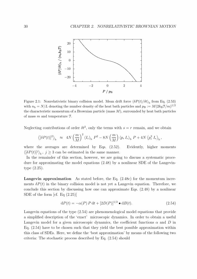
Figure 2.1 depicts the mean drift force 〈δP (t)/δt〉b, obtained from Eq. (2.53). The absolute
value of this drift force grows linearly for small momentum values (Ornstein-Uhlenbeck
regime) and quadratically for large momentum values.
We still consider the second moment:
⟨
[δP (t)]2⟩
b= 4
(m
M
)2N
∑
s=1
N∑
r=1
〈IrIs〉b P 2 − 8(m
M
)
N∑
s=1
N∑
r=1
〈pr IrIs〉b P +
4
N∑
r=1
N∑
s=1
〈prps Ir Is〉b .
30 CHAPTER 2. NONRELATIVISTIC BROWNIAN MOTION
−20
−10
0
10
20
〈δP/δt〉
b/
(nbkBT)
〈δP/δt〉
b/
(nbkBT)
−4 −2 0 2 4
P / pBP / pB
Figure 2.1: Nonrelativistic binary collision model. Mean drift force 〈δP (t)/δt〉b from Eq. (2.53)
with nb = N/L denoting the number density of the heat bath particles and pB := M(2kBT/m)1/2
the characteristic momentum of a Brownian particle (mass M), surrounded by heat bath particles
of mass m and temperature T.
Neglecting contributions of order δt2, only the terms with s = r remain, and we obtain
⟨
[δP (t)]2⟩
b≈ 4N
(m
M
)2
〈Ir〉b P 2 − 8N(m
M
)
〈pr Ir〉b P + 4N⟨
p2r Ir
⟩
b,
where the averages are determined by Eqs. (2.52). Evidently, higher moments
〈[δP (t)]j〉b , j ≥ 3 can be estimated in the same manner.
In the remainder of this section, however, we are going to discuss a systematic proce-
dure for approximating the model equations (2.48) by a nonlinear SDE of the Langevin-
type (2.25).
Langevin approximation As stated before, the Eq. (2.48c) for the momentum incre-
ments δP (t) in the binary collision model is not yet a Langevin equation. Therefore, we
conclude this section by discussing how one can approximate Eqs. (2.48) by a nonlinear
SDE of the form [cf. Eq (2.25)]
dP (t) = −α(P )P dt+ [2D(P )]1/2 • dB(t). (2.54)
Langevin equations of the type (2.54) are phenomenological model equations that provide
a simplified description of the ‘exact’ microscopic dynamics. In order to obtain a useful
Langevin model for a given microscopic dynamics, the coefficient functions α and D in
Eq. (2.54) have to be chosen such that they yield the best possible approximation within
this class of SDEs. Here, we define the ‘best approximation’ by means of the following two
criteria: The stochastic process described by Eq. (2.54) should

2.2. MICROSCOPIC MODELS 31
• approach the correct stationary momentum distribution for the Brownian particle;
• be characterized by the same mean relaxation (drift) behavior as Eq. (2.48c).
The first criterion is equivalent to imposing the appropriate fluction-dissipation relation
on the functions α and D. For the elastic collision model considered here, the expected
stationary momentum PDF is given by the Maxwell distribution
φ∞(p) = (2πMkBT)−1/2 exp(
−p2/[2MkBT])
. (2.55)
According to the discussion in Section 2.1.2, this implies that α and D must be coupled
by the Einstein condition
D(P ) = α(P )MkBT. (2.56)
The second (drift) criterion can be expressed mathematically as13
⟨
dP (t)
dt
∣
∣
∣
∣
P (t) = p
⟩
!=
⟨
δP (t)
δt
∣
∣
∣
∣
P (t) = p
⟩
b
. (2.57)
The rhs. of Eq. (2.57) may be determined from Eq. (2.53), yielding the mean drift force
g(p) :=
⟨
δP (t)
δt
∣
∣
∣
∣
P (t) = p
⟩
b
= −2nbkBT
{
π−1/2
(
p
pB
)
exp
[
−(
p
pB
)2]
+
[
(
p
pB
)2
+1
2
]
erf
(
p
pB
)}
. (2.58a)
In order to evaluate the lhs. of Eq. (2.57), we note that for the post-point discretization
rule (•) it is known that [cf. (C.25)]
⟨
[2D(P )]1/2 • dB(t) | P (t) = p⟩
= D′(p) dt,
where the prime denotes the derivative with respect to the momentum variable. Substi-
tuting the Einstein relation (2.56), i.e., D(p) = α(P )MkBT, we obtain
⟨
[2D(P )]1/2 • dB(t) | P (t) = p⟩
= α′(p)M kBT dt.
Combining this with the conditional expectation for the friction term in Eq. (2.54),
〈−α(P )P dt | P (t) = p〉 = −α(p) p dt,
13We denote by 〈 |P (t) = p〉 the conditional expectation with respect to the Wiener measure of the
Brownian motion B(t).
32 CHAPTER 2. NONRELATIVISTIC BROWNIAN MOTION
we find for the lhs. of Eq. (2.57) the result
⟨
dP (t)
dt
∣
∣
∣
∣
P (t) = p
⟩
= −[α(p) p− α′(p) M kBT], (2.58b)
Hence, by virtue of Eqs. (2.58), we see that the drift criterion (2.57) is equivalent to the
following ordinary differential equation (ODE) for α(p):
−α(p) p + α′(p) M kBT = g(p). (2.59)
With respect to the two criteria formulated above, the solution of this ODE yields the
friction function α that provides the ‘best’ Langevin approximation to the binary collision
model. Information about the collision model and the bath distribution is encoded in the
mean drift force g(p). Evidently, the procedure leading to Eq. (2.59) can be generalized to
other interaction models/bath distributions as well – provided the stationary distribution
of the Brownian particle is known. Other types of interactions (e.g., nonelastic) would
result in another function g(p). A non-Maxwellian bath distribution would affect not only
the rhs. of Eq. (2.59) but also its lhs. due to a modified fluctuation-dissipation relation.
In order to analyze Eq. (2.59) for our specific collision model, it is useful to define rescaled
dimensionless quantities
p∗ := p/pB, µ∗ := m/M, α∗(p∗) := α(p) /(2nbkBT/pB),
allowing us to rewrite Eq. (2.59) in the form
α∗(p∗) p∗ −µ∗
2α′∗(p∗) =
p∗π1/2
exp(−p2∗) +
(
p2∗ +
1
2
)
erf(p∗). (2.60)
This linear inhomogeneous first order ODE can be solved by standard numerical methods,
but one still needs to specify an initial condition, e.g., the value α∗(0). The correct choice
of α∗(0) can, in principle, be determined from the expected asymptotic behavior of α∗(p∗)
at large momentum values |p∗| → ∞. Considering the limit |p∗| → ∞, we find that the
solutions of Eq. (2.60) must converge to the solutions of the following asymptotic ODE
α∗(p∗) p∗ −µ∗
2α′∗(p∗) =
(
p2∗ +
1
2
)
sign(p∗). (2.61)
The general solution of Eq. (2.61) with initial value α∗(0) reads
α∗(p∗) = |p∗| + ep2∗/µ∗
[
α∗(0) − π1/2
2
(
µ1/2∗ + µ−1/2
∗
)
erf(
µ−1/2∗ |p∗|
)
]
. (2.62)
The asymptotic solution (2.62) implies that the friction coefficient α would grow or decrease
exponentially unless one chooses a particular initial condition. Hence, the physically correct
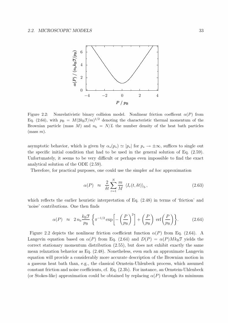
2.2. MICROSCOPIC MODELS 33
0
2
4
6
α(P
)/
(nbkBT/p
B)
α(P
)/
(nbkBT/p
B)
−4 −2 0 2 4
P / pBP / pB
Figure 2.2: Nonrelativistic binary collision model. Nonlinear friction coefficent α(P ) from
Eq. (2.64), with pB = M(2kBT/m)1/2 denoting the characteristic thermal momentum of the
Brownian particle (mass M) and nb = N/L the number density of the heat bath particles
(mass m).
asymptotic behavior, which is given by α∗(p∗) ≃ |p∗| for p∗ → ±∞, suffices to single out
the specific initial condition that had to be used in the general solution of Eq. (2.59).
Unfortunately, it seems to be very difficult or perhaps even impossible to find the exact
analytical solution of the ODE (2.59).
Therefore, for practical purposes, one could use the simpler ad hoc approximation
α(P ) ≈ 2
δt
N∑
r=1
m
M〈Ir(t, δt)〉b , (2.63)
which reflects the earlier heuristic interpretation of Eq. (2.48) in terms of ‘friction’ and
‘noise’ contributions. One then finds
α(P ) ≈ 2nbkBT
pB
{
π−1/2 exp
[
−(
P
pB
)2]
+
(
P
pB
)
erf
(
P
pB
)}
. (2.64)
Figure 2.2 depicts the nonlinear friction coefficient function α(P ) from Eq. (2.64). A
Langevin equation based on α(P ) from Eq. (2.64) and D(P ) = α(P )MkBT yields the
correct stationary momentum distribution (2.55), but does not exhibit exactly the same
mean relaxation behavior as Eq. (2.48). Nonetheless, even such an approximate Langevin
equation will provide a considerably more accurate description of the Brownian motion in
a gaseous heat bath than, e.g., the classical Ornstein-Uhlenbeck process, which assumed
constant friction and noise coefficients, cf. Eq. (2.3b). For instance, an Ornstein-Uhlenbeck
(or Stokes-like) approximation could be obtained by replacing α(P ) through its minimum
34 CHAPTER 2. NONRELATIVISTIC BROWNIAN MOTION
value
α(0) = nbm
M
(
2kBT
πm
)1/2
, (2.65a)
D(0) = α(0) M kBT. (2.65b)
Adopting this additional simplification, the corresponding Ornstein-Uhlenbeck process can
be expected to provide a useful description for slow Brownian particles at sufficiently low
temperature values T.
Although not quite as rigorous as the derivation from the harmonic oscillator model in
Section 2.2.1, the collision model provides useful insights into the approximations that must
be made in order to obtain a Langevin equation from a microscopic model. Compared with
the oscillator model, a main advantage of the collision model is given by the fact that it
can be extended to special relativity, cf. discussion in Section 4.3.
Chapter 3
Relativistic equilibrium
thermostatistics
The preceding discussion of the nonrelativistic Brownian motion theory has shown that
equilibrium thermostatistics plays an important role in constraining the relation between
friction and noise coefficients in Langevin equations. Therefore, the present chapter intends
to clarify several aspects of relativistic equilibrium thermostatistics. These considerations
will become relevant in Chapter 4, when we will have to specify the fluctuation-dissipation
relations for the relativistic Langevin theory.
Evidently, the nonrelativistic Brownian motion models from Chapter 2 are in conflict
with special relativity because they do not prevent particles from moving faster than the
speed of light c. For example, the stationary velocity distribution of the classical, e.g.,
Ornstein-Uhlenbeck process (2.1) is given by a Maxwell distribution that is non-zero for
velocities |v| > c. Hence, if one wants to construct a relativistic version of the Ornstein-
Uhlenbeck process then one has to know the relativistic generalization of the Maxwell
distribution first. The recent literature has seen considerable debate about the correct gen-
eralization of Maxwell’s velocity distribution in special relativity [14,16,203,211,215,216].
In Sec. 3.2 we shall present results of fully relativistic 1D molecular dynamics simula-
tions [17] which clearly favor a distribution that was proposed by Juttner [167] in 1911,
i.e., six years after Einstein had formulated his theory of special relativity [2,3]. Moreover,
as discussed in the last part of this chapter, our simulations can also be used to illustrate
the meaning of temperature and thermal equilibrium in special relativity [17].
35
36 CHAPTER 3. RELATIVISTIC EQUILIBRIUM THERMOSTATISTICS
3.1 Preliminaries
Section 3.1.1 contains a brief summary of the definitions and the notation that will be used
in the remainder. Subsequently, the ‘peculiar’ transformation behavior of one-particle
phase space PDFs under Lorentz transformations will be addressed. For simplicity, we
restrict ourselves to discussing the 1D case (i.e., one time dimension and one space dimen-
sion); the corresponding generalization to higher space dimensions is straightforward.
3.1.1 Notation and conventions
The position of point-like particle in the inertial lab frame Σ at lab time t is denoted
by X(t); its lab velocity is defined by V (t) := dX(t)/dt. The relativistic momentum P (t)
and the relativistic particle energy E(t) with respect to Σ are given by
P (t) := cM V (t) γ(V (t)) , E(t) := c2M γ(V (t)), (3.1)
with M > 0 denoting the particle rest mass and Lorentz factor
γ(v) :=(
1 − v2/c2)−1/2
. (3.2)
To keep the subsequent formulas as simple as possible, we will from now on adopt a natural
unit system with c = 1 yielding, e.g., the simplified relations
P = EV = MV γ(V ) , E = (M2 + P 2)1/2 = Mγ(V ). (3.3)
Time and position, and energy and momentum can be combined into the contravariant
four-vectors1
(Xα) := (t, X), (P α) := (E, P ), α = 0, 1. (3.4)
The components Xα and Pα of the corresponding covariant four-vectors are defined by
Xα := ηαβXβ, Pα := ηαβP
β, (ηαβ) = diag(−1, 1). (3.5)
Here, ηαβ denote the components of the Minkowski metric tensor, and Einstein’s summation
convention has been used, i.e.,
ηαβXβ :=
∑
β
ηαβXβ.
The above definitions refer to the inertial lab frame Σ. Now consider a second inertial
frame Σ′, moving with velocity w relative to Σ. According to Einstein’s theory of special
1We shall use the term ‘four-vector’ regardless of the actual number of spatial dimensions. Contravariant
(covariant) four-vectors will be treated as column (row) vectors.
3.1. PRELIMINARIES 37
relativity, values of physical quantities in Σ′ can be related to those in Σ by means of a
Lorentz transformation [6, 8]. In the 1D case, the corresponding Lorentz transformation
matrix reads
Λ(w) = γ(w)
(
1 −w−w 1
)
= (Λ(w)αβ). (3.6)
The inverse Λ−1(w) is equal to Λ(−w). The transformation law of an arbitrary four-vector
(Aα) reads A′α = Λ(w)αβA
β, leading in the case of (Xα) and (P α) to the explicit results
(
t′
X ′
)
= γ(w)
(
t− wX
−wt +X
)
,
(
E ′
P ′
)
= γ(w)
(
E − wP
−wE + P
)
. (3.7)
The rest mass M of a particle is Lorentz invariant, i.e.,
M = (E2 − P 2)1/2 = (−PαPα)1/2 = (−P ′
αP′α)1/2 = (E ′2 − P ′2)1/2 = M ′.
Throughout, we will assume that the rest mass of a particle is not changed by interactions.
Finally, considering a particle with velocity curve V (t), its Lorentz invariant proper time
span ∆τ , elapsing between coordinate times t1 and t2, is given by
∆τ :=
∫ t2
t1
dt [1 − V (t)2]1/2 ⇔ dτ := dt [1 − V (t)2]1/2. (3.8)
3.1.2 Probability densities in special relativity
With regard to the subsequent discussion, it is worthwhile to clarify the definition and
transformation behavior of PDFs in special relativity. The results presented in this sub-
section were proven rigorously by van Kampen [138].
To start with, we consider the one-particle phase space PDF f(t, x, p) ≥ 0, where the
coordinates (t, x, p) refer to the lab frame Σ with p = mγ(v)v denoting the relativistic
kinetic momentum. For a relativistic many-particle system (e.g., a gas) with conserved
particle number N ≫ 1, the function f can be defined operationally as follows [138]:
If an observer O, who is at rest in Σ, observes the system at Σ-time t, he finds
N f(t, x, p) dxdp
particles in the phase space interval [x, x + dx] × [p, p + dp]. Alternatively, when con-
sidering the random motion of a single Brownian particle in a fluctuating medium, the
quantity f(t, x, p)dxdp gives the probability of finding the Brownian particle at lab time t
in [x, x + dx] × [p, p+ dp]. In either case, the function f is subject to the t-simultaneous
normalization condition
1 =
∫
dxdp f(t, x, p). (3.9)
38 CHAPTER 3. RELATIVISTIC EQUILIBRIUM THERMOSTATISTICS
Now consider a second observer O′, moving with velocity w 6= 0 relative to Σ. The ob-
server O′ will measure another distribution f ′(t′, x′, p′) and one is led to wonder how the two
functions f ′(t′, x′, p′) and f(t, x, p) are related to each other. In the nonrelativistic theory,
the change from one inertial system to another does not affect the time coordinate; hence,
one can use the standard transformation laws for PDFs in that case [see, e.g., Eq. (2.17)].
By contrast, in the relativistic case the situation becomes more complicated, because now
the definition of f and f ′ is based on an observer-dependent notion of simultaneity. Put dif-
ferently, the measurements of O and O′ refer to the two different hyperplanes “t=constant”
and “t′=constant” in Minkowski space, respectively. Van Kampen [138] was able to prove
that the one-particle phase space density f transforms as a Lorentz scalar, i.e.,2
f(t, x, p) = f ′(t′, x′, p′), (3.10)
where (t, x, p) and (t′, x′, p′) are connected by a Lorentz transformation with velocity param-
eter w. Moreover, he showed that the function f ′ satisfies the t′-simultaneous normalization
condition
1 =
∫
dx′dp′ f(t′, x′, p′). (3.11)
Van Kampen’s proof [138] of Eq. (3.10) uses an assumption about the uniqueness of particle
trajectories and a reparameterization of the particles trajectories in terms of their invariant
proper times. As a consequence, Eq. (3.10) represents a generic kinematical result and
applies to a broad class of interaction models.
We next summarize several useful implications of Eq. (3.10). For this purpose, we define
the marginal densities
φ(t, p) =
∫
dx f(t, x, p), φ′(t′, p′) =
∫
dx′ f ′(t′, x′, p′), (3.12a)
(t, x) =
∫
dp f(t, x, p), ′(t′, x′) =
∫
dp′ f ′(t′, x′, p′). (3.12b)
Then the following statements hold true [138]:
(i) Free particles. An unconfined system consisting of free, identical particles of rest mass
m (i.e., no interactions, no external fields, no walls) is described by a time-independent
marginal momentum distribution φ(p). In this case, one finds
(m2 + p2)1/2 φ(p) = (m2 + p′2)1/2 φ′(p′). (3.13)
2One can find several insufficient ‘proofs’ of Eq. (3.10) in the literature, cf. the discussion in [138,201].
In this context it is often claimed, erroneously, that the phase space element dxdp is a Lorentz scalar; in
Section 2 of their paper, Debbasch et al. [201] demonstrate in detail that this is not true in general.
3.1. PRELIMINARIES 39
(ii) Ideal gas in a container. Consider a spatially homogeneous gas enclosed in a box
that rests in the lab frame Σ. Assume that the gas is in equilibrium and can be described
by a time-independent one-particle phase space density
f(x, p) =φ(p)
VI(x)
in Σ, where V is the rest volume of the box in Σ and I(x) the indicator for the box, i.e.,
I(x) = 1 if x is within the box and I(x) = 0, otherwise. In this case, Eq. (3.10) implies
that3
φ(p)
V=φ′(p′)
V ′, (3.14)
where V ′ = V/γ(w) is the Lorentz-contracted box volume in the moving frame Σ′. At first
sight it is surprising that the presence of the box alters the transformation properties of the
momentum distribution. However, this can be explained by the fact that the observations
by O and O′ are not synchronous, and that in the time between their observations some
particles collide with the container walls.4
(iii) Current-density vector. The quantities
(t, x) =
∫
dp f(t, x, p) , j(t, x) =
∫
dp v f(t, x, p) (3.15)
can be combined into a current-density four-vector (jα) = (, j), since they transform as
′(t′, x′) = γ(w) (t, x) − γ(w)w j(t, x), (3.16a)
j′(t′, x′) = −γ(w)w (t, x) + γ(w) j(t, x). (3.16b)
Furthermore, it can be shown that jα satisfies the continuity equation
∂αjα =
∂
∂t+ divj = 0. (3.17)
Equation (3.10) and statements (i)− (iii) remain valid in higher space dimensions d > 1
upon replacing x → x, p → p, j → j, etc. [138]. Moreover, Eq. (3.10) can be generalized
to the case of N -particle phase space PDFs fN , yielding for arbitrary space dimensions
fN (t1,x1,p1; . . . ; tN ,xN ,pN) = f ′N(t′1,x
′1,p
′1; . . . ; t
′N ,x
′N ,p
′N ), (3.18)
where for n = 1, . . . , N the coordinates (t′n,x′n,p
′n) and (tn,xn,pn) are connected by a
Lorentz-transformation, and fN is the multiple-time probability density for lab observer O
to observe particle 1 at time t1 near (x1,p1), and particle 2 at time t2 near (x2,p2), etc..
The above results clarify the transformation behavior of PDFs in special relativity, but
they do not yet answer the question as to which PDF provides the correct description for
a given physical system as, e.g., a relativistic gas in equilibrium. The latter problem will
be addressed in the next part.
3This result was already derived by Dirac [453] in 1924.4Cf. discussion in Section 6 of van Kampen’s paper [138].
40 CHAPTER 3. RELATIVISTIC EQUILIBRIUM THERMOSTATISTICS
3.2 Thermostatistics of a relativistic gas
The recent literature has seen considerable debate about the correct generalization of
Maxwell’s velocity distribution in special relativity [14, 16, 203, 211, 215, 216]. Knowing
the correct equilibrium velocity distributions of relativistic many-particle systems is es-
sential for a proper interpretation of experiments in high energy and astrophysics [312,
314, 317, 338]. Examples include thermalization processes in heavy ion collision exper-
iments [312, 314] and ultra-relativistic plasma beams [338], or the relativistic Sunyaev-
Zel’dovich (SZ) effect [317], describing the distortion of the cosmic microwave background
(CMB) radiation spectrum due to the interaction of CMB photons with hot electrons
in clusters of galaxies [454–456]. The predicted strength of the spectral distortions and
the cosmological parameters inferred from the SZ effect depend on the assumed velocity
distribution of the relativistic electrons [317].
The equilibrium velocity distribution of a relativistic gas does also play an important
role in the context of relativistic Brownian motion theory. As mentioned before, when
postulating relativistic Langevin equations [10,11,18,334], this distribution must be known
in advance in order to correctly specify the relativistic fluctuation-dissipation relation.
Furthermore, the relativistic equilibrium velocity distribution is required as an input, if one
wants to derive relativistic Langevin-type equations from a microscopic collision model.
3.2.1 Relative entropy, Haar measures and canonical velocity
distributions
At the beginning of the last century it was commonly accepted that the one-particle velocity
distribution of a dilute (quasi-ideal) gas in equilibrium is described by the Maxwellian (2.51)
ψM(v;m, β, d) =
(
βm
2π
)d/2
exp
(
−βmv2
2
)
, (3.19)
where m is the rest mass of a gas particle, v ∈ Rd the velocity, T = (kBβ)−1 the tem-
perature, and d the number of space dimension. After Einstein [2, 3] had formulated his
theory of special relativity in 1905, Planck and others noted immediately that the distribu-
tion (3.19) is in conflict with the fundamental relativistic postulate that velocities cannot
exceed the light speed c. A first solution to this problem was put forward by Ferencz
Juttner [167] in 1911. He proposed the following relativistic generalization of Maxwell’s
PDF [167]:
ψJ(v;m, βJ, d) =md
ZJγ(v)2+d exp[−βJmγ(v)], |v| < 1, (3.20a)
with ZJ = ZJ(m, βJ, d) being the normalization constant, and ψJ ≡ 0 if |v| ≥ 1. Assuming
a spatially homogeneous gas distribution, Eq. (3.20a) corresponds to the one-particle phase
3.2. THERMOSTATISTICS OF A RELATIVISTIC GAS 41
space PDF5
fJ(x,p) = (ZJV )−1 exp[−βJE(p)], (3.20b)
where V is the volume of the gas container, E(m,p) = (m2+p2)1/2 = mγ(v) the relativistic
particle energy, and p = mvγ(v) the relativistic momentum; the corresponding marginal
momentum PDF reads6
φJ(p) = Z−1J exp[−βJE(p)]. (3.20c)
Equations (3.20) refer to a lab frame Σ where the box, enclosing the gas, is at rest.
Juttner’s proposal (3.20) became widely accepted among theorists during the first three
quarters of the last century [112,162,169,273,289] – although a rigorous microscopic deriva-
tion remained lacking due to the difficulty of formulating a relativistically consistent Hamil-
ton mechanics of interacting particles [223, 224, 226, 228, 252]. Doubts about the Juttner
function fJ began to arise in the 1980s, when Horwitz et al. [215, 216] suggested a ‘man-
ifestly covariant’ relativistic Boltzmann equation, whose stationary solution differs from
Eq. (3.20) and, in particular, predicts a different mean energy-temperature relation in the
ultra-relativistic limit [206]. Since then, partially conflicting results and proposals from
other authors [14,16,203,207,211] have led to an increasing confusion as to which distribu-
tion actually represents the correct generalization of the Maxwellian (3.19). For example,
another recently discussed alternative to Eq. (3.20), which also reduces to the Maxwell
distribution in the nonrelativistic limit case, is the ‘modified’ Juttner function [14,16,211]
ψMJ(v;m, βMJ, d) =md
ZMJ
γ(v)2+d
mγ(v)exp[−βMJmγ(v)]. (3.21a)
For a spatially homogeneous gas, Eq. (3.21a) corresponds to the phase space PDF
fMJ(x,p) = V −1φMJ(p), (3.21b)
with marginal momentum density
φMJ(p) =(ZMJ)−1
E(p)exp[−βMJE(p)], (3.21c)
Compared with the Juttner distribution (3.20) at the same parameter values
βJ = βMJ . 1/m, the modified PDFs (3.21) exhibits a significantly lower particle popu-
lation in the high energy tail because of the additional 1/E-prefactor.
5Here and below, it will be assumed that f vanishes outside the gas container.6Juttner [167] derived the distribution (3.20) from a maximum entropy principle; cf. Section 3.2.1. An
alternative derivation based on the microscopic ensemble is given by Matolcsi et al. [198].
42 CHAPTER 3. RELATIVISTIC EQUILIBRIUM THERMOSTATISTICS
Maximum relative entropy principle In a recent paper [16] we have demonstrated
that the distributions (3.20) and (3.21) can be obtained from a common maximum relative
entropy principle by using different reference densities, respectively. To briefly illustrate
this, we return to the 1D case7 d = 1 and consider two positive density functions φ(p) > 0
and ρ(p) > 0 on the 1D relativistic momentum space8 RM1 = (−∞,∞). The functions
φ and ρ define two measures [457] µφ and µρ, respectively, upon assigning to any subset
A ⊆ RM1 the numbers9
µφ(A) :=
∫
A
dp φ(p) , µρ(A) :=
∫
A
dp ρ(p). (3.22)
The relative entropy S of φ with respect to ρ (or, equivalently, of µφ with respect to µρ)
is defined by [458–460]
S[φ|ρ] := −∫
dp φ(p) lnφ(p)
ρ(p). (3.23)
Here, as usual, the symbol∫
dp signals an integration with respect to the Lebesgue mea-
sure λ on RM1 = (−∞,∞), which assigns to each interval A = [a, b] ⊆ R the intuitive
measure number [457]
λ(A) =
∫
A
dp =
∫ b
a
dp = b− a.
It is worthwhile to note that the relative entropy (3.23) is manifestly invariant under coor-
dinate transformations [16]. In the mathematical literature, the definition of the relative
entropy is often given in the form
S[µφ|µρ] := −∫
dµφ lndµφ
dµρ, (3.24)
which upon identifying
dµφ = dp φ(p) , dµρ = dp ρ(p) ,dµφ
dµρ=φ(p)
ρ(p)
becomes equivalent to Eq. (3.23). The relative entropy is also known as the Kullback-
Leibler entropy [461], and the non-negative functiondµφ
dµρ(p) is the Radon-Nikodym den-
sity [457] of µφ with respect to µρ. In the remainder, we are going to work with the density
representation (3.23).
7See Ref. [16] for a discussion of the d-dimensional case.8Since we restrict ourselves to the spatially homogeneous case, it suffices to focus on the momentum
distribution φ.9In particular, if µφ(RM1) = 1 holds true then φ ≥ 0 is a PDF and µφ a probability measure on RM1;
at this point, however, we do not require normalization of φ or ρ.
3.2. THERMOSTATISTICS OF A RELATIVISTIC GAS 43
The relative entropy S[φ|ρ] from Eq. (3.23) constitutes the basis of the maximum rela-
tive entropy principle. This principle formalizes the idea that, for a broad class of physical
systems, the canonical equilibrium distribution can be obtained by maximizing an appro-
priate entropy functional in the presence of constraints. The constraints encode a priori
knowledge about the system. In our case, we are interested in maximizing S[φ|ρ] with
respect to φ under the conditions
1 =
∫
dp φ(p), (3.25a)
ǫ =
∫
dp E(p)φ(p). (3.25b)
The first constraint (3.25a) ensures that φ is a PDF. The second constraint (3.25b) reflects
the assumption that the mean energy per particle, ǫ, is known. These constraints may be
incorporated into the maximum entropy principle via the method of Lagrangian multipli-
ers [462]. Denoting the Lagrangian multipliers by (α, β), the maximum entropy principle
results the necessary condition
0 ≡ δ
δφ
{
S[φ|ρ] + α
[
1 −∫
dp φ(p)
]
+ β
[
ǫ−∫
dp E(p)φ(p)
]}∣
∣
∣
∣
φ=φ∗
= −[
1 + lnφ∗(p)
ρ(p)
]
− α− βE(p), (3.26)
whose solution is readily obtained as10
φ∗(p) = (p) exp[
−(1 + α) − βE(p)]
. (3.27)
The Lagrangian multipliers (α, β) can be determined from the two conditions (3.25) yield-
ing, e.g., β as a function of the given mean value ǫ. Moreover, it is evident now that
normalization of the reference density ρ is irrelevant, since constant prefactors will be
absorbed by the multiplier α. We next discuss three specific cases:
a) Maxwell distribution. Upon choosing a constant reference density in momentum
space, ρ(p) = ρ0, and the nonrelativistic kinetic energy E(p) = p2/(2m), the solu-
tion (3.27) yields the 1D nonrelativistic Maxwell momentum distribution (2.16).
b) Juttner distribution. Fixing again a constant reference density, ρ(p) ≡ ρ0, and consid-
ering the relativistic energy E(p) = (m2 + p2)1/2, one recovers Juttner’s momentum
PDF (3.20c).
10Due to the appearance of the logarithm, the maximization of the entropy functional (3.23) gives rise
to an ‘exponential’ distribution (3.27). By considering other non-logarithmic ‘entropies’ like, e.g., Tsallis’
or Kaniadakis’ entropy, one may construct other forms of distributions (e.g., power law distributions).
44 CHAPTER 3. RELATIVISTIC EQUILIBRIUM THERMOSTATISTICS
c) Modified Juttner distribution. Considering, as in b), the relativistic energy
E(p) = (m2 + p2)1/2, but now with a non-constant reference density ρ(p) = E(p)−1
in Eq. (3.27), one obtains the modified Juttner PDF (3.21c).
This shows that the two candidate distribution (3.20) and (3.21) may be derived from a
common maximum relative entropy principle, but they refer to different reference densities
(i.e., reference measures), respectively. It is worthwhile to clarify the difference between
the two reference measures by analyzing their respective symmetries:
The constant reference density ρ(p) ≡ ρ0, underlying the Juttner distribution (3.20),
corresponds to the Lebesgue measure λ on RM1, i.e., in this case we have
µρ(A) = ρ0 λ(A) , ∀ A ∈ RM1 = R. (3.28)
The associated relative entropy
S[φ|ρ0] := −∫
dp φ(p) lnφ(p)
ρ0(3.29)
coincides with the usual Shannon-Boltzmann-Gibbs entropy on RM1. The Lebesgue mea-
sure λ on RM1 is distinguished by the fact that it is the only translation invariant measure
on the relativistic momentum space. Here, translation invariance of λ means that
λ([a+ x, b + x]) = (b+ x) − (a + x) = b− a = λ([a, b])
holds for all a, b, x ∈ RM1. In more mathematical terms, λ represents the Haar measure11
of the (additive) momentum translation group (RM1,+).
11In a seminal paper [463] published in 1933, the Hungarian mathematician Alfred Haar studied the
possibility to introduce a measure µ◦ on a continuous group (G, ◦) such that µ◦ is invariant under the group
multiplication ‘◦’. To briefly sketch this idea, consider a subset A of the group G and some arbitrary, fixed
group element g ∈ G. By multiplying each element a ∈ A with g, the subset A is mapped onto another
subset of G, denoted by
g ◦ A := {g ◦ a |a ∈ A } .
Now consider a measure µ◦ on G that assigns to A ⊆ G some non-negative real number µ◦(A). The
measure µ◦ is said to be group invariant, if
µ◦(g ◦ A) = µ◦(A)
holds for any g ∈ G and A ⊆ G. In the case of non-commutative (i.e., non-Abelian) groups, one may
distinguish invariance under multiplications from the right or left. Haar [463] was able to prove the
existence of an invariant measure µ◦, and its uniqueness apart from an irrelevant multiplicative constant
for locally compact, topological groups. Such group invariant measures µ◦ are referred to as Haar measures
nowadays [457]. They give a mathematically precise meaning to the notion ‘uniform distribution’ by
combining measure and group theoretical concepts.
3.2. THERMOSTATISTICS OF A RELATIVISTIC GAS 45
Now consider the reference density ρ(p) = E(p)−1, which yields the modified momentum
PDF (3.21c). We may define the Lorentz transformation L[A] of a set A ⊂ RM1 by
L[A] := {L(p) | p ∈ A} . (3.30)
By taking into account the well-known fact that [138, 290]
dp
E(p)=
dp′
E(p′)(3.31)
holds under Lorentz transformations, one then finds that
µρ(L[A]) = µρ(A) , ∀ A ∈ RM1. (3.32)
That is, the measure µρ induced by ρ(p) = E(p)−1 is invariant under Lorentz transforma-
tions.
To briefly summarize, adopting the Lebesgue measure in momentum space as reference
measure yields the Juttner function (3.20c), whereas the Lorentz invariant reference mea-
sure yields the modified distribution (3.21c). Hence, at this stage, both distribution func-
tions appear to be plausible candidates,12 and it remains the question which reference
measure is the physically correct one. This question cannot be answered on the level of
the maximum entropy principle and, therefore, other approaches have to be explored. To
identify the physically correct distribution, we have performed numerical simulations of a
fully relativistic dynamical 1D gas model that will be discussed in the next section.
3.2.2 Relativistic molecular dynamics simulations
To resolve the uncertainty about the relativistic one-particle equilibrium velocity PDF, we
performed fully relativistic 1D molecular dynamics (MD) simulations in collaboration with
David Cubero and Jesus Casado from the Universidad de Sevilla [17]. The restriction to the
1D case is inevitable if one wants to treat localized particle interactions in a relativistically
consistent manner, cf. the remarks below. In our computer experiments we simulated the
dynamics of classical, impenetrable point-particles with elastic point-like binary collisions,
employing an algorithm similar to those of Alder and Wainwright [464] and Masoliver and
Marro [465].
12As shown in [14], the modified distribution satisfies an additional elastic collision invariance criterion;
this microscopic criterion, however, does not take into account the collision rates and is, therefore, not
appropriate for determining the equilibrium distribution of a confined system as, e.g., a relativistic gas in
a container.
46 CHAPTER 3. RELATIVISTIC EQUILIBRIUM THERMOSTATISTICS
The basic time step of the algorithm involves three partial tasks:
(i) determine the next collision event (xc, tc);
(ii) evolve the system up to time tc;
(iii) calculate the momenta after the collision.
The third task is solved as follows: If two particles A and B meet at the space-time point
(xc, tc), then they exchange momentum according to the relativistic energy momentum
conservation laws
pA + pB = pA + pB, (3.33a)
E(mA, pA) + E(mB, pB) = E(mA, pA) + E(mB, pB), (3.33b)
where E(m, p) = (m2 + p2)1/2 is the relativistic particle energy. Given the momenta
(pA, pB) before the collision, these conservation laws determine the momenta (pA, pB) after
the collision by [14]
pA = γ(u)2[2uE(mA, pA) − (1 + u2)pA], (3.34a)
pB = γ(u)2[2uE(mB, pB) − (1 + u2)pB], (3.34b)
where
u = (pA + pB)/[E(mA, pA) + E(mB, pB)]
is the collision-invariant, relativistic center-of-mass velocity of the two particles. By as-
suming strictly localized, point-like pair interactions, one may avoid the introduction of
fields which are required when considering relativistic particle interactions-at-a-distance.13
However, considering point-like localized interactions is expedient in the 1D case only; in
higher space dimension the collision probability would become zero, thus preventing the
system from equilibration. Moreover, if two colliding particles carry the same rest masses
then elastic 1D collisions merely interchange their velocities; hence, elastic binary collisions
are not able to drive a 1D one-component gas to equilibrium. In our simulations we consid-
ered a two-component mixture, consisting of N1 light particles with equal masses m1, and
N2 heavy particles with equal masses m2 > m1. The motion of the N = N1 +N2 particles
was restricted to the 1D interval [0, L], assumed to be stationary in the lab frame Σ. The
numerical results presented below refer to elastic reflections at the boundaries; however,
we found that periodic boundary conditions yield identical outcomes if the total initial
momentum was chosen to be zero in Σ. Generally, our simulations mimic a relativistic
13The interested reader may wish to consult the original papers of Wheeler and Feynman [223], Currie
et al. [226], and Van Dam and Wigner [224, 225], who discuss in detail the difficulties associated with
classical particle-particle interactions in special relativity.
3.2. THERMOSTATISTICS OF A RELATIVISTIC GAS 47
microcanonical ensemble, since the total initial energy Etot in Σ is conserved in the mi-
croscopic collision processes. The above conventions define the simplest interacting model
system that
a) complies with all principles of special relativity,
b) does not require the introduction of interaction fields,
c) can be simulated without further approximation, and
d) exhibits a universal stationary equilibrium state.
Hence, this simple model is well-suited for probing the predictions of different relativistic
kinetic theories [162,169,206,215,273,289] by means of numerical experiments. Moreover,
as we shall see below, this model may help to clarify longstanding questions regarding the
definition and meaning of ‘temperature’ and ‘thermal equilibrium’ in special relativity.
Numerical results In order to identify the stationary one-particle velocity distributions
for the light and heavy particles, respectively, we waited until the 1D two-component gas
had approached the equilibrium state (typically, after 102 collisions per particle). Then the
particle velocities were measured Σ-simultaneously, i.e., at equal time t with respect to the
resting lab frame Σ. To increase the sample size we repeated this procedure several times
during a simulation run and collected the data into a single histogram. An example is shown
in Fig. 3.1, based on a simulation with N = 2000 particles (N1 = N2 = 1000, m2 = 2m1).
Each particle was given a random initial position xi(0) ∈ [0, L] and a random initial velocity
vi(0) = ±0.8, corresponding to a mean energy per particle ǫ = Etot/(N1 + N2) = 2.5m1.
As evident from Fig. 3.1, for both particle species the numerically obtained one-particle
PDFs (◦) are in very good agreement with the standard Juttner function ψJ (solid line),
and differ significantly from the modified distribution ψMJ (dashed lines).
The distribution parameters βJ/MJ underlying the graphs in Fig. 3.1 were determined
from the initial energy by means of the following consideration: If the particle numbers N1
and N2 are sufficiently large (thermodynamic limit), then the one-particle PDFs in the lab
frame Σ are expected to converge to either ψJ from Eq. (3.20a) or ψMJ from Eq. (3.21a).
Generally, the mean relativistic energy value ǫ of a one-particle velocity PDF ψ(v;m, β) is
defined by
ǫ(m, β) =
∫
{|v|<1}
ddv ψ(v;m, β) mγ(v). (3.35)
Assuming that (i) an equilibrium state exists where both species can be described by the
same value β, and that (ii) for a gas in equilibrium the mean energy per particle is the
same for particles of the same species, the total energy can be expressed as
Etot = N1 ǫ(m1, β) +N2 ǫ(m2, β). (3.36)
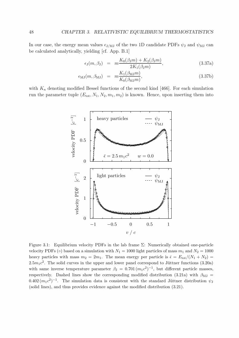
48 CHAPTER 3. RELATIVISTIC EQUILIBRIUM THERMOSTATISTICS
In our case, the energy mean values ǫJ/MJ of the two 1D candidate PDFs ψJ and ψMJ can
be calculated analytically, yielding [cf. App. B.1]
ǫJ(m, βJ) = mK0(βJm) +K2(βJm)
2K1(βJm), (3.37a)
ǫMJ(m, βMJ) = mK1(βMJm)
K0(βMJm), (3.37b)
with Kn denoting modified Bessel functions of the second kind [466]. For each simulation
run the parameter tuple (Etot, N1, N2, m1, m2) is known. Hence, upon inserting them into
light particles
0
1
2
vel
oci
tyP
DF
[c−
1]
−1 −0.5 0 0.5 1
v / c
ψJ
ψMJ
heavy particles
ǫ = 2.5m1c2 w = 0.0
0
0.5
1
vel
oci
tyP
DF
[c−
1]
ψJ
ψMJ
Figure 3.1: Equilibrium velocity PDFs in the lab frame Σ: Numerically obtained one-particle
velocity PDFs (◦) based on a simulation with N1 = 1000 light particles of mass m1 and N2 = 1000
heavy particles with mass m2 = 2m1. The mean energy per particle is ǫ = Etot/(N1 + N2) =
2.5m1c2. The solid curves in the upper and lower panel correspond to Juttner functions (3.20a)
with same inverse temperature parameter βJ = 0.701 (m1c2)−1, but different particle masses,
respectively. Dashed lines show the corresponding modified distribution (3.21a) with βMJ =
0.402 (m1c2)−1. The simulation data is consistent with the standard Juttner distribution ψJ
(solid lines), and thus provides evidence against the modified distribution (3.21).
3.2. THERMOSTATISTICS OF A RELATIVISTIC GAS 49
Eqs. (3.36) and (3.37), these parameters uniquely determine the parameter value βJ/MJ
that is consistent with the chosen velocity PDF fJ/MJ.
Temperature and thermal equilibrium in special relativity Remarkably, in spite
of the different particle masses the two numerically obtained velocity PDFs in Fig. 3.1 are
very well matched by Juttner functions (3.20) with the same parameter βJ. According to
our simulations, this holds true with high accuracy for a wide range of initial conditions
and mass ratios. Hence, the Juttner function does not only provide the best ‘fit’ to the
numerical data, it also yields a well-defined concept of ‘temperature’ in special relativity:
Intuitively, the temperature T is thought to be an intensive quantity that equilibrates to a
common value if two or more systems are brought into contact with each other (i.e., may
exchange different forms of energy). In our case, it is natural to consider the particle species
as two different subsystems that may exchange energy via elastic collision processes. After
a certain relaxation time, the combined system approaches a ‘thermodynamic equilibrium
state’, where each subsystem is described by the same asymptotic, two-parametric velocity
PDF ψJ(v;mi, βJ), differing only via the rest masses mi. The commonly shared distribution
parameter βJ may thus be used to define a relativistic equilibrium temperature by
T := (kBβJ)−1. (3.38)
However, for this concept to be meaningful, a restriction of the accessible spatial volume
is required – be it by means of periodic boundary conditions, or by imposing reflecting
walls.14 Otherwise, it cannot be expected that a many-particle system approaches a uni-
versal stationary state which is independent of the specific initial conditions. This obser-
vation has an important implication: Any (relativistic or non-relativistic) Boltzmann-type
equation [206, 215, 216, 273, 289, 290, 292] that gives rise to a universal stationary velocity
PDF implicitly assumes the presence of a spatial confinement, thus singling out a preferred
frame of reference.
14The critical role of the boundary conditions in relativistic systems has been emphasized by
Sinyukov [467] and van Kampen [137,138]. Loosely speaking, if a many-particle system has reached a uni-
versal stationary equilibrium state, then each particle ‘knows’ about the presence of the confinement/walls
because equilibration typically requires momentum reversal at the walls, e.g., in order to maintain a uni-
form density and a well-balanced average collision frequency. In particular, if the walls are considered to
be stationary objects then they single out a preferred frame of reference. The relevance of the boundary
conditions is even more obvious in quantum mechanics/statistics due to their direct effect on the energy
spectra and, thus, on the density of states. In fact, quantum mechanical arguments [170] suggest ρ(p) ≡ ρ0
in Eq. (3.23).
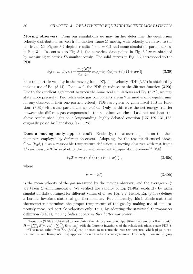
50 CHAPTER 3. RELATIVISTIC EQUILIBRIUM THERMOSTATISTICS
Moving observers From our simulations we may further determine the equilibrium
velocity distributions as seen from another frame Σ′ moving with velocity w relative to the
lab frame Σ. Figure 3.2 depicts results for w = 0.2 and same simulation parameters as
in Fig. 3.1. In contrast to Fig. 3.1, the numerical data points in Fig. 3.2 were obtained
by measuring velocities Σ′-simultaneously. The solid curves in Fig. 3.2 correspond to the
ψ′J(v′;m, βJ, w) =
mγ(v′)3
ZJ γ(w)exp[−βJγ(w)mγ(v′) (1 + wv′)] (3.39)
[v′ is the particle velocity in the moving frame Σ′]. The velocity PDF (3.39) is obtained by
making use of Eq. (3.14). For w = 0, the PDF ψ′J reduces to the Juttner function (3.20).
Due to the excellent agreement between the numerical simulations and Eq. (3.39), we may
state more precisely: Two relativistic gas components are in ‘thermodynamic equilibrium’
for any observer if their one-particle velocity PDFs are given by generalized Juttner func-
tions (3.39) with same parameters βJ and w. Only in this case the net energy transfer
between the different gas components in the container vanishes. Last but not least, the
above results shed light on a longstanding, highly debated question [127, 129–131, 158]
originally posed by Landsberg [126, 128]:
Does a moving body appear cool? Evidently, the answer depends on the ther-
mometers employed by different observers. Adopting, for the reasons discussed above,
T := (kBβJ)−1 as a reasonable temperature definition, a moving observer with rest frame
Σ′ can measure T by exploiting the Lorentz invariant equipartition theorem15 [128]
kBT = mγ(w)3⟨
γ(v′) (v′ + w)2⟩′, (3.40a)
where
w = −〈v′〉′ (3.40b)
is the mean velocity of the gas measured by the moving observer, and the averages 〈 · 〉′are taken Σ′-simultaneously. We verified the validity of Eq. (3.40a) explicitly by using
simulation data obtained for different values of w, see Fig. 3.3. Hence, Eq. (3.40a) defines
a Lorentz invariant statistical gas thermometer. Put differently, this intrinsic statistical
thermometer determines the proper temperature of the gas by making use of simulta-
neously measured particle velocities only; thus, by adopting the statistical thermometer
definition (3.40a), moving bodies appear neither hotter nor colder.16
15Equation (3.40a) is obtained by combining the microcanonical equipartition theorem for a Hamiltonian
H =∑N1
i=1E(m1, pi) +
∑N2
j=1E(m2, pj) with the Lorentz invariance of the relativistic phase space PDF f .
16The mean value from Eq. (3.40a) can be used to measure the rest temperature, which plays a cen-
tral role in van Kampen’s [137] approach to relativistic thermodynamics. Evidently, upon multiplying
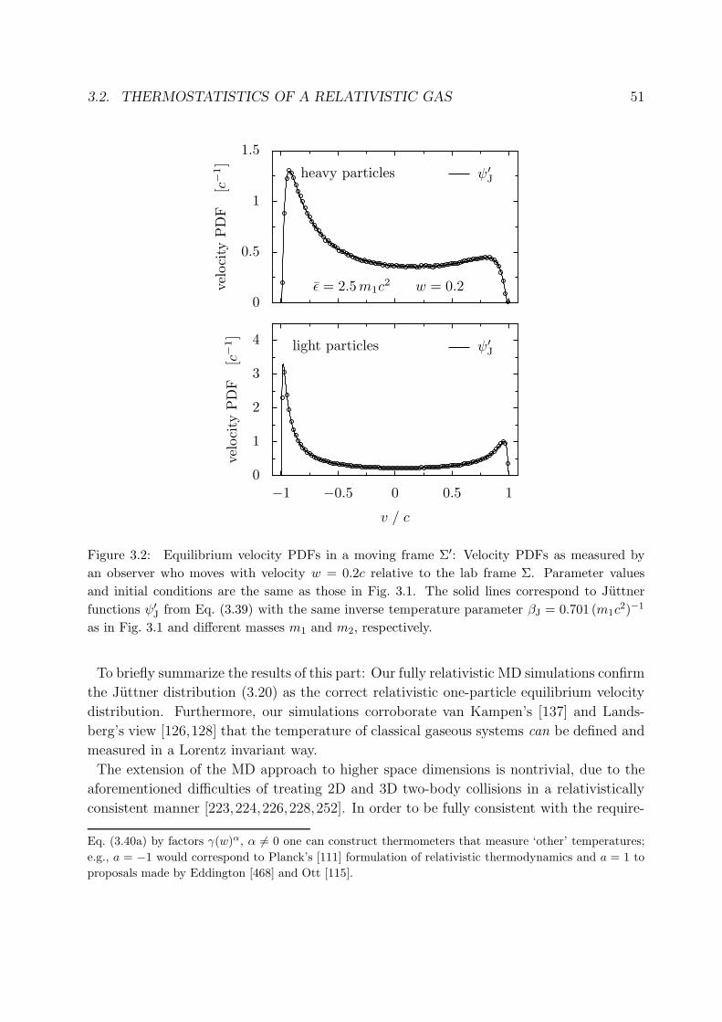
3.2. THERMOSTATISTICS OF A RELATIVISTIC GAS 51
light particles
0
1
2
3
4
vel
oci
tyP
DF
[c−
1]
−1 −0.5 0 0.5 1
v / c
ψ′
J
heavy particles
ǫ = 2.5m1c2 w = 0.2
0
0.5
1
1.5
vel
oci
tyP
DF
[c−
1]
ψ′
J
Figure 3.2: Equilibrium velocity PDFs in a moving frame Σ′: Velocity PDFs as measured by
an observer who moves with velocity w = 0.2c relative to the lab frame Σ. Parameter values
and initial conditions are the same as those in Fig. 3.1. The solid lines correspond to Juttner
functions ψ′J from Eq. (3.39) with the same inverse temperature parameter βJ = 0.701 (m1c
2)−1
as in Fig. 3.1 and different masses m1 and m2, respectively.
To briefly summarize the results of this part: Our fully relativistic MD simulations confirm
the Juttner distribution (3.20) as the correct relativistic one-particle equilibrium velocity
distribution. Furthermore, our simulations corroborate van Kampen’s [137] and Lands-
berg’s view [126,128] that the temperature of classical gaseous systems can be defined and
measured in a Lorentz invariant way.
The extension of the MD approach to higher space dimensions is nontrivial, due to the
aforementioned difficulties of treating 2D and 3D two-body collisions in a relativistically
consistent manner [223,224,226,228,252]. In order to be fully consistent with the require-
Eq. (3.40a) by factors γ(w)α, α 6= 0 one can construct thermometers that measure ‘other’ temperatures;
e.g., a = −1 would correspond to Planck’s [111] formulation of relativistic thermodynamics and a = 1 to
proposals made by Eddington [468] and Ott [115].
52 CHAPTER 3. RELATIVISTIC EQUILIBRIUM THERMOSTATISTICS
−0.6
−0.4
−0.2
0
〈v′〉′/c
0 0.2 0.4 0.6
w / c
1.2
1.4
1.6
kBT/
(m1c2
)
0 0.2 0.4 0.6
w / c
Figure 3.3: Measured mean particle velocity (◦, left digram) and estimated temperature (◦, right
diagram) based on Eqs. (3.40) as a function of the observer velocity w. Solid lines correspond to
the theoretically expected values, respectively, using the same simulation parameters and initial
conditions as in Fig. 3.2.
ments of special relativity, relativistic 2D/3D interactions must be formulated in terms of
fields. Unfortunately, direct simulation of the field dynamics is numerically expensive and,
therefore, practically unfeasible in most cases. Alternatively, one can use simplified semi-
relativistic models such as, e.g., effective hard-sphere models where the interaction radius
is defined with respect the center-of-mass frame of the colliding particles [469]. Generally,
it can be expected that such simplified models yield satisfactory results in the low den-
sity regime, but they may lead to inconsistencies at high densities, e.g., when three-body
encounters become relevant.
We conclude this part with another general remark: The above results correspond the case
where an ‘ordinary’ thermal equilibrium state is approached, corresponding to a stationary
exponential one-particle momentum distributions. For completeness we note that, in gen-
eral, one can also imagine non-equilibrium scenarios that give arise to (quasi-)stationary
distributions which differ from the Juttner function;17 see, e.g., Kaniadakis [203,208,209],
Silva and Lima [207,210], Lina et al. [213], or Beck [204]. However, our subsequent discus-
sion of relativistic Langevin equations will focus on the case, where the heat bath, which
surrounds the Brownian particle, is described by a spatially homogeneous Juttner function.
17Typical examples are unconfined systems with a limited number of collisions per particle as, e.g., in
an expanding dilute gas.
Chapter 4
Relativistic Brownian motion
The present chapter discusses the generalization of the Langevin theory of Brownian mo-
tions to the framework of special relativity [10, 11, 13, 14, 16, 18–24, 331, 333–335, 374, 470].
More precisely, we will consider stochastic differential equations (SDEs) that describe
Markov processes in relativistic one-particle phase space.1 Relativistic Langevin equa-
tions present a useful tool for modeling the dynamics of relativistic particles in a ran-
dom environment. Recently, for example, SDEs have been applied to analyze thermal-
ization effects in quark-gluon plasmas produced at the Relativistic Heavy Ion Collider
(RHIC) [312–314, 337].2 The subsequent sections intend to give a comprehensive discus-
sion and illustration of the underlying mathematical theory.
The phenomenological or axiomatic Langevin approach to relativistic Brownian motion
was initiated by Debbasch et al. [18], who in 1997 proposed a simple relativistic generaliza-
tion of the classical Ornstein-Uhlenbeck process [36]. The relativistic Ornstein-Uhlenbeck
process (ROUP) of Debbasch et al. [18] is obtained by postulating additive white noise for
the particle’s momentum change in the rest frame of the bath. During the past decade
various properties of the ROUP were studied by Debbasch and Rivet [19,20], Barbachoux
et al. [21,22], and Zygad lo [334]. An alternative approach to relativistic Langevin equations
was pursued by us in Refs. [10, 11]. By starting from a ‘Newtonian’ Ornstein-Uhlenbeck-
type Langevin equation in the comoving rest frame of a Brownian particle, we obtained
a modified relativistic Brownian motion (RBM) process, whose relaxation behavior differs
from that of the ROUP. As we are going to illustrate below, the two different processes
represent special limit cases of a larger class of relativistic Langevin models [12], which
may be used to describe the random motions of relativistic particles.
The content of the present chapter is structured as follows. Section 4.1 discusses the
axiomatic Langevin approach, i.e., suitable SDEs and fluctuation-dissipation relations are
1As discussed by Lopuszanski [339], Dudley (Theorem 11.3 in [341]) and Hakim (Proposition 2 in [346]),
it is impossible to define nontrivial relativistic Markov processes in position space.2Potential applications in high energy astrophysics are discussed by Dieckmann et al. [338] and [471].
53
54 CHAPTER 4. RELATIVISTIC BROWNIAN MOTION
postulated in order to provide a simplified model of the complex interaction between the
Brownian particle and its environment (heat bath). After having outlined the general
conceptual foundations (Section 4.1.1), specific examples are considered (Section 4.1.2).
In Section 4.1.3, we will analyze the temperature dependence of the asymptotic mean
square displacement for different example processes, using general analytic formulas re-
cently derived by Lindner [24], and Angst and Franchi [23]. In particular, we are going
to demonstrate that the diffusion constant is sensitive with respect to variations of the
friction coefficients. This result implies that measurements of the diffusion constant may
reveal information about the underlying microscopic interactions. Section 4.2 discusses
relativistic Brownian motion processes from the viewpoint of a moving observer. In the
last part of this chapter (Section 4.3), we will generalize the binary collision model from
Section 2.2.2 to the relativistic case in order to obtain a simple microscopic model for
relativistic Brownian motions.
4.1 Langevin and Fokker-Planck equations
Roughly speaking, a relativistic Brownian motion process is a stochastic process whose
absolute velocity |V (t)| does not exceed the speed of light c at any time. Of particular
interest for our subsequent discussion are stochastic processes which
(i) satisfy the condition |V (t)| < c, and
(ii) can be modeled by means of Langevin-type SDEs, or, equivalently, by means of
Fokker-Planck equations (FPEs).
When considering Langevin equations as models of Brownian motion, one implicitly as-
sumes that it is possible and reasonable to separate the degrees of freedom of the Brownian
particle from those of the environment (heat bath). Adopting this point of view, one can
specify two distinguished frames of reference: the stationary inertial rest frame Σ of the
heat bath, and the inertial frame Σ∗ that is comoving with the Brownian particle at a
given instant of time.3 As before, Σ is referred to as lab frame. In the present section, we
focus on describing relativistic Brownian motion processes with respect to the space-time
coordinates of Σ.
3Apart from an irrelevant shift of the origin, the inertial lab frame Σ is uniquely determined by the
requirement that the mean velocity of the heat bath particles, which is assumed to be constant in any
inertial frame, must vanish in Σ. Similarly, the instantaneously comoving frame Σ∗ is determined by
the condition that the Σ∗-velocity of the Brownian particle is equal to zero at the given instant of time.
Generally, we assume that the time coordinates t and t∗ can be measured, e.g., by using atomic clocks
that are at rest in Σ or Σ∗, respectively.
4.1. LANGEVIN AND FOKKER-PLANCK EQUATIONS 55
4.1.1 Construction principle and conceptual aspects
The basic idea for constructing stochastic processes that meet the criteria (i) and (ii)
is to postulate Langevin equations for the relativistic momentum coordinates P = (P i),
i = 1, . . . , d which can take values in R = (−∞,+∞). This automatically prevents particle
velocities from exceeding the speed of light, because the associated absolute velocity
|V | =|P |P 0
=|P |
(M2 + P 2)1/2
is always less than c = 1 (throughout, M > 0 denotes the rest mass of the Brownian
particle). However, before we can actually write down specific Langevin equations for
the relativistic momentum components P i, an important question needs to be addressed,
namely, the choice of the time parameter in relativistic Langevin equations.
Choice of the time parameter A fundamental assumption (postulate) of nonrelativis-
tic Galilean physics is the existence of a universal time t. Hence, within the nonrelativistic
Langevin theory, it seems very natural to identify this universal time t with the time pa-
rameter of the stochastic driving process, often taken to be a multi-dimensional Wiener
process B(t), cf. Eq. (2.3b). By contrast, in special relativity the notion of time is
frame-dependent. Consequently, it becomes important to specify in advance which time
parameter is used to quantify the fluctuations of the underlying stochastic driving process.
When considering the stochastic motion of a relativistic Brownian particle, two distin-
guished time parameters exist: The coordinate time t of the inertial lab frame Σ, defined
as the mean rest frame of the stationary heat bath, and the proper time τ of the Brownian
particle. In principle, either of the two parameters could be used to formulate SDEs for
the spatial components of the particle momentum, P = (P i). However, within the con-
ventional Langevin picture of Brownian motion, one usually considers friction and noise as
externally imposed forces that act upon the Brownian particle. Therefore, it seems more
natural to characterize the statistical properties of the noise source in terms of the lab
time t.4
Accordingly, within this lab time approach [10, 11, 18, 19, 21, 22, 333, 334, 472], one aims
primarily at constructing 2d-dimensional relativistic stochastic processes {X(t),P (t)} with
respect to the lab frame Σ, where the position coordinates X = (X i) and the spatial
momentum coordinates P = (P i) are connected by the standard relativistic differential
4Within this lab time approach, the proper time becomes a stochastic quantity, and one could, for
example, ask for the probability of finding at lab time t the particle’s proper time in the interval [τ, τ+dτ ].
Conversely, if adopting the proper time τ as the primary deterministic evolution parameter, one could ask
for the probability to find the particle at proper time τ within the space-time interval [t, t+dt]× [x,x+dx]
with respect to the lab frame.
56 CHAPTER 4. RELATIVISTIC BROWNIAN MOTION
relation
dX i(t) = V i dt = (P i/P 0) dt, i = 1, . . . , d, (4.1)
with P 0(t) = (M2 + P 2)1/2 denoting the relativistic energy. Stochasticity is implemented
into the dynamics by coupling the momentum components P i(t) to an external noise
source via an SDE. Below, we shall focus on the case where the noise source is modeled by
a standard Wiener process. Analogous to the nonrelativistic case, the relativistic Langevin
equation (RLE) for the stochastic increments dP i(t) can be written using different kinds
of discretization rules. In the following, we will consider the three most popular cases,
corresponding to the post-point (•), mid-point (◦) and pre-point rule (∗), respectively.
From now on, we concentrate again on the one-dimensional case d = 1. This is sufficient
for clarifying the basic concepts and ideas. The generalization to higher space-dimensions
is straightforward and summarized in App. D.
Post-point discretization Similar to the nonrelativistic case, we postulate that the a
momentum change dP (t) of the relativistic Brownian particle in the lab frame Σ (= rest
frame of the bath) can be modeled by a Langevin equation of the from5
dP (t) = −α•(P )P dt+ [2D(P )]1/2 • dB(t), (4.2a)
where B(t) is a standard Wiener process with increment PDF (2.3d). If the background
medium (heat bath) is stationary and spatially homogeneous, then both the friction co-
efficient α and the noise amplitude D should depend on the relativistic particle energy
E(P ) = (M2 + P 2)1/2 only, i.e.,
α•(p) = α•(E) , D(p) = D(E). (4.2b)
In the remainder, we will always assume that Eqs. (4.2b) hold true. An additional con-
straint results from the requirement that Eq. (4.2a) should yield the correct stationary
momentum distribution.
The FPE for the phase space density f(t, x, p) of a relativistic Brownian particle, governed
by Eq. (4.1) with d = 1 and Eq. (4.2a), reads
∂f
∂t+p
E
∂f
∂x=
∂
∂p
[
α•(p) p f +D(p)∂f
∂p
]
. (4.2c)
Analogous to Eq. (2.27), the corresponding stationary distribution is given by6
f∞(x, p) = N exp
[
−∫ p
p∗
dp′α•(p
′)
D(p′)p′
]
. (4.2d)
5In principle, one could also consider other driving process (as, e.g., Levy or Poisson processes) and/or
coefficient functions α(t,X, P ) and D(t,X, P ).6Here, we assume the presence of a spatial confinement or periodic boundary conditions.
4.1. LANGEVIN AND FOKKER-PLANCK EQUATIONS 57
The arbitrary boundary value p∗ is absorbed by the normalization constant N. Upon
demanding that the marginal momentum distribution φ∞(p) be given by the relativistic
Juttner function φJ(p) ∝ exp[−βE(p)], we obtain the condition
α•(p)
D(p)p
!≡ − d
dplog φJ(p) =
d
dpβE(p). (4.2e)
Hence, by using dE(p)/dp = p/E(p), we find
α•(p)
D(p)≡ β
E(p). (4.2f)
This is the relativistic fluctuation-dissipation relation, also referred to as the relativistic
Einstein relation. Compared with the nonrelativistic Einstein relation (2.29), the mass has
been replaced with energy on the rhs. of Eq. (4.2f).
Furthermore, it is straightforward to derive from Eq. (4.2a) the corresponding SDE for the
relativistic energy P 0 = E(P ) = (M2+P 2)1/2. Applying the (backward) Ito formula (C.27)
with Y = P , Z = P 0 and G(p) = (M2 + p2)1/2, we obtain the following SDE for the
relativistic energy P 0 = E(P ):
dP 0(t) =
{
−α•(P0)P 0
[
1 −(
M
P 0
)2]
− D(P 0)
P 0
(
M
P 0
)2}
dt+
{
2 D(P 0)
[
1 −(
M
P 0
)2]}1/2
• dB(t), (4.2g)
where α•(P ) = α•(P0) and D(P ) = D(P 0).
Mid-point discretization The relativistic Langevin equation (4.2a) may be rewritten
in terms of an equivalent Stratonovich-Fisk SDE, reading
dP (t) = −α◦(P )P dt+ [2D(P )]1/2 ◦ dB(t), (4.3a)
where the friction coefficient functions α◦ and α• are related by [cf. Eq. (C.43)]7
α◦(p) p = α•(p) p−D′(p)/2 (4.3b)
and D′(p) := dD(p)/dp. The relativistic Einstein relation (4.2f), reexpressed in terms of
α◦(p), reads
α◦(p) ≡βD(p)
E(p)− 1
2
D′(p)
p, (4.3c)
7See also the corresponding discussion by Hanggi [473], and Hanggi and Thomas (page 293 of Ref. [67]).

58 CHAPTER 4. RELATIVISTIC BROWNIAN MOTION
i.e., only if α◦(p) and D(p) satisfy the criterion (4.3c), then the stationary momentum
distribution is given by Juttner’s PDF. Moreover, if D and α• depend on the relativistic
particle energy P 0 = E only, i.e., if D(p) = D(E) and α•(p) = α•(E) hold true, then we
may write
D′(p) = (p/E) D′(E)
where D′(E) := dD(E)/dE. In this case, Eq. (4.3b) becomes equivalent to
α◦(p) = α•(E) − D′(E)/(2E) =: α◦(E), (4.3d)
and the Einstein relation (4.3c) can be rewritten in the form
α◦(E) ≡ [2βD(E) − D′(E)]/(2E). (4.3e)
The rules of ordinary differential calculus are preserved for Stratonovich-Fisk SDEs. Con-
sequently, we find the following Stratonovich-Fisk SDE for the energy P 0 = E(P ):
dP 0(t) = −α◦(P0)P 0
[
1 −(
M
P 0
)2]
dt+
{
2 D(P 0)
[
1 −(
M
P 0
)2]}1/2
◦ dB(t). (4.3f)
Pre-point discretization The relativistic Langevin equations (4.2a) and (4.3a) can also
be rewritten in terms of the equivalent Ito SDE
dP (t) = −α∗(P )P dt+ [2D(P )]1/2 ∗ dB(t), (4.4a)
where the friction coefficients α∗ and α• are related by [cf. Eq. (C.43)]
α∗(p) p = α•(p) p−D′(p). (4.4b)
Compared with Eqs. (4.2a) and (4.3a), the Ito SDE (4.4) is most convenient for numerical
simulations. For a homogeneous isotropic bath with D(p) = D(E) and α•(p) = α•(E),
Eq. (4.4b) is equivalent to
α∗(p) = α•(E) − D′(E)/E =: α∗(E), (4.4c)
and the relativistic Einstein relation becomes
α∗(E) ≡ [βD(E) − D′(E)]/E. (4.4d)
4.1. LANGEVIN AND FOKKER-PLANCK EQUATIONS 59
Applying the Ito formula (C.10), we obtain the following Ito SDE for the energy P 0
dP 0(t) =
{
−α∗(P0)P 0
[
1 −(
M
P 0
)2]
+D(P 0)
P 0
(
M
P 0
)2}
dt+
{
2 D(P 0)
[
1 −(
M
P 0
)2]}1/2
∗ dB(t). (4.4e)
Having outlined the general ideas underlying the axiomatic Langevin approach to relativis-
tic Brownian motions in the lab frame, we next consider several example processes.
4.1.2 Examples
We discuss three specific 1D relativistic Langevin models whose stationary momentum
distributions are given by the Juttner function φJ(p) = exp[−βE(p)]. In this case, the
relativistic Einstein relation (4.2f) implies that only one of the two functions α•(p) and
D(p) can be chosen arbitrarily.
Constant noise amplitude As a first example, we consider the so-called ’Relativistic
Ornstein-Uhlenbeck process’ (ROUP), proposed by Debbasch et al. [18,19] and also studied
by Zygad lo [334]. The ROUP is defined by the choice
α•(p) = αc M/E(p), (4.5a)
where αc > 0 is a constant friction parameter. From the relativistic Einstein relation (4.2f),
one then finds
D(p) ≡ α•(p)E(p)β−1 = αcM β−1 = αcM kBT =: Dc, (4.5b)
i.e., the ROUP corresponds to the limit case of constant noise amplitude. The associated
Langevin equation reads
dP (t) = −αcM
P 0P dt+
(
2αcM
β
)1/2
• dB(t) (4.5c)
= −αcM
P 0P dt+
(
2αcM
β
)1/2
∗ dB(t). (4.5d)
The discretization rule is irrelevant here, because the noise amplitude Dc = αcM/β does
not depend on the momentum P for this particular case. However, the rules of stochastic
calculus have to be specified, if one wishes to write down the SDE for the associated velocity
60 CHAPTER 4. RELATIVISTIC BROWNIAN MOTION
process V (t) := P/P 0. For example, adopting the post-point discretization, the Langevin
equation for V (t) reads
dV (t) = −αc
[
(1 − V 2)3/2 − 3kBT
M(1 − V 2)2
]
V dt+
[
2αckBT
M(1 − V 2)3
]1/2
• dB(t). (4.5e)
For comparison, the corresponding Ito SDE is given by
dV (t) = −αc
[
(1 − V 2)3/2 +3kBT
M(1 − V 2)2
]
V dt+
[
2αckBT
M(1 − V 2)3
]1/2
∗ dB(t). (4.5f)
Constant friction coefficient in the backward-Ito SDE An alternative relativistic
Brownian motion (RBM) model, considered by us in Ref. [10,11], corresponds to the special
case of a constant friction function α•(p) ≡ α† in the backward-Ito SDE (4.2a). In this case,
the relativistic Einstein relation (4.2f) yields the momentum dependent noise amplitude
D(p) = α†E(p) β−1. (4.6a)
Adopting the post-point discretization scheme, the relativistic Langevin equation of this
model reads
dP (t) = −α† P dt+
(
2α†P0
β
)1/2
• dB(t). (4.6b)
The corresponding SDE for the velocity process V (t) = P/P 0 is given by
dV (t) = −α†
[
(1 − V 2) − 3kBT
M(1 − V 2)3/2
]
V dt+
[
2αckBT
M(1 − V 2)5/2
]1/2
• dB(t). (4.6c)
Recently, various properties of the RBM process (4.6b) have been analyzed by Fa [331],
Lindner [24], Fingerle8 [470], and Angst and Franchi [23].
With regard to numerical simulations,9 the Ito form of Eqs. (4.6b) is often more conve-
nient. By making use of Eq. (4.4c), the equivalent Ito SDEs are obtained as
dP (t) = −α†
(
βP 0 − 1
βP 0
)
P dt +
(
2α†P0
β
)1/2
∗ dB(t), (4.6d)
8Fingerle [470] discusses a fluctuation theorem for this process; see also Cleuren et al. [218].9Cf. App. C.
4.1. LANGEVIN AND FOKKER-PLANCK EQUATIONS 61
and
dV (t) = −α†
[
(1 − V 2) +2kBT
M(1 − V 2)3/2
]
V dt +
[
2αckBT
M(1 − V 2)5/2
]1/2
∗ dB(t). (4.6e)
Constant friction coefficient in the Ito-SDE The RBM process defined by Eq. (4.6b)
is characterized by a constant friction coefficient α†, when adopting the post-point dis-
cretization rule (•). Another model, referred to as RBM(I) hereafter, is obtained by con-
sidering a constant friction coefficient α∗ in the Ito-Langevin equation
dP (t) = −α∗ P dt+
[
2α∗
β2(1 + βP 0)
]1/2
∗ dB(t), (4.7a)
where the noise amplitude is chosen such that the Einstein relation (4.4d) is satisfied. For
completeness, the Ito-SDE of the associated velocity process V (t) := P/P 0 is given by
dV (t) = −α∗
[
(1 − V 2) + 3kBT
M(1 − V 2)3/2 + 3
(
kBT
M
)2
(1 − V 2)2
]
V dt+
{
2α∗kBT
M
[
(1 − V 2)5/2 +kBT
M(1 − V 2)3
]}1/2
∗ dB(t). (4.7b)
The three model processes (4.5d), (4.6b) and (4.7a) give rise to the same stationary
momentum PDF φJ(p), but their respective relaxation behavior differs strongly. This
is illustrated in Fig. 4.1, which depicts the time evolution of the spatial mean square
displacement divided by time,
Dt :=⟨
[X(t) −X(0)]2⟩
/(2t), (4.8)
for all three models at same temperature T. The curves in Fig. 4.1 were calculated numer-
ically from Eqs. (4.5d), (4.6d) and (4.7a), respectively, using an algorithm similar to those
described in [23, 24], see also App. C.5.
4.1.3 Asymptotic mean square displacement
A primary objective within any Brownian theory is to determine the asymptotic diffusion
constant D∞, corresponding to the plateau values in Fig. 4.1. For a 1D diffusion process
X(t) with velocity V (t), the asymptotic diffusion constant D∞ is defined by
D∞ = limt→∞
⟨
[X(t) −X(0)]2⟩
/(2t), (4.9a)
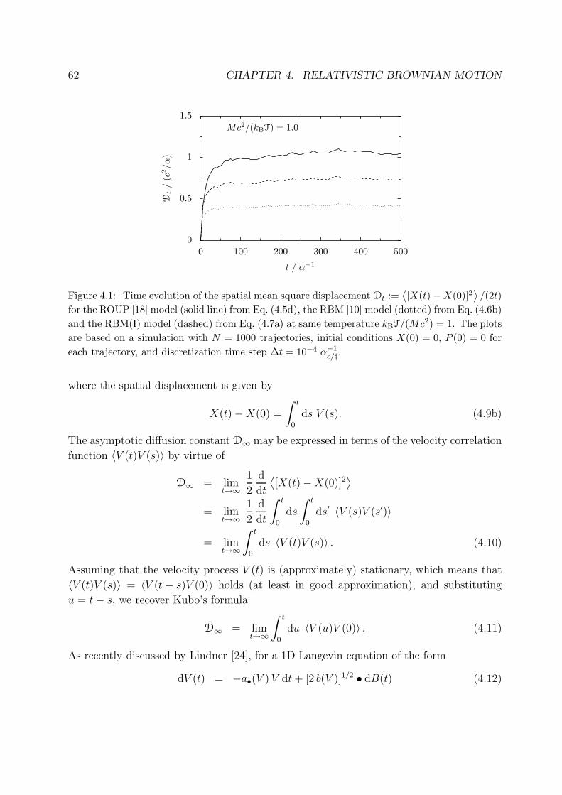
62 CHAPTER 4. RELATIVISTIC BROWNIAN MOTION
Mc2/(kBT) = 1.0
0
0.5
1
1.5
Dt/
(c2/α
)
0 100 200 300 400 500
t / α−1
Figure 4.1: Time evolution of the spatial mean square displacement Dt :=⟨
[X(t) −X(0)]2⟩
/(2t)
for the ROUP [18] model (solid line) from Eq. (4.5d), the RBM [10] model (dotted) from Eq. (4.6b)
and the RBM(I) model (dashed) from Eq. (4.7a) at same temperature kBT/(Mc2) = 1. The plots
are based on a simulation with N = 1000 trajectories, initial conditions X(0) = 0, P (0) = 0 for
each trajectory, and discretization time step ∆t = 10−4 α−1c/†.
where the spatial displacement is given by
X(t) −X(0) =
∫ t
0
ds V (s). (4.9b)
The asymptotic diffusion constant D∞ may be expressed in terms of the velocity correlation
function 〈V (t)V (s)〉 by virtue of
D∞ = limt→∞
1
2
d
dt
⟨
[X(t) −X(0)]2⟩
= limt→∞
1
2
d
dt
∫ t
0
ds
∫ t
0
ds′ 〈V (s)V (s′)〉
= limt→∞
∫ t
0
ds 〈V (t)V (s)〉 . (4.10)
Assuming that the velocity process V (t) is (approximately) stationary, which means that
〈V (t)V (s)〉 = 〈V (t− s)V (0)〉 holds (at least in good approximation), and substituting
u = t− s, we recover Kubo’s formula
D∞ = limt→∞
∫ t
0
du 〈V (u)V (0)〉 . (4.11)
As recently discussed by Lindner [24], for a 1D Langevin equation of the form
dV (t) = −a•(V )V dt+ [2 b(V )]1/2 • dB(t) (4.12)
4.1. LANGEVIN AND FOKKER-PLANCK EQUATIONS 63
with symmetric coefficient functions, a•(v) = a•(−v) and b(v) = b(−v), the Kubo for-
mula (4.11) gives rise to the following integral representation for the asymptotic diffusion
constant:10
D∞ =
∫ v+
0dy eU(y)
[
∫ v+
ydx e−U(x) x/b(x)
]2
∫ v+
0dz e−U(z)/b(z)
. (4.13)
Here, v+ ∈ [0,∞] represents the upper bound for the velocity range, and
U(v) :=
∫ v
0
dw µ∗(w)/b(w) (4.14a)
is an effective velocity potential with Ito drift
µ∗(v) := a∗(v) v = a•(v) v − b′(v). (4.14b)
In general, the formula (4.13) has to be integrated numerically, but for the first two models
from Section 4.1.2 the integrals may also be evaluated analytically.
For example, upon comparing with Eq. (4.6e), we see that the RBM model from Eq. (4.6b)
is described by
µ∗(v) = α†
[
(1 − v2) +2kBT
M(1 − v2)3/2
]
v, (4.15a)
b(v) = α†kBT
M(1 − v2)5/2, (4.15b)
with an upper velocity bound v+ = c = 1. In this case, the rhs. of Eq. (4.13) can be
calculated analytically by making use of the identity
(−1)ν dν
dχνK0(χ) =
∫ 1
0
dv exp
(
− χ√1 − v2
)
(1 − v2)−(ν+2)/2, (4.16)
where, for ν = 0, 1, 2 . . ., Kν(z) denotes the modified Bessel function of the second
kind [466]. One then finds that11
DRBM∞ = (α†βM)−1 K0(βM)
K1(βM). (4.17)
At low temperatures β := (kBT)−1 → ∞, Eq. (4.17) reduces to the well-known classical
result Dclass∞ = kBT/(Mα†), cf. Eq. (2.20). In the opposite limit of very high temperatures,
i.e., for βM ≪ 1, one finds a logarithmic dependence [23]
DRBM∞ = (α†M)−1
{
−γǫ + ln[ 2
βM
]
+ O[(βM)2]
}
, (4.18)
10A d-dimensional generalization of Eq. (4.13) was recently derived by Angst and Franchi [23].11Equation (4.17) is an equivalent, more compact representation of Lindner’s result Eq. (10) in [24].
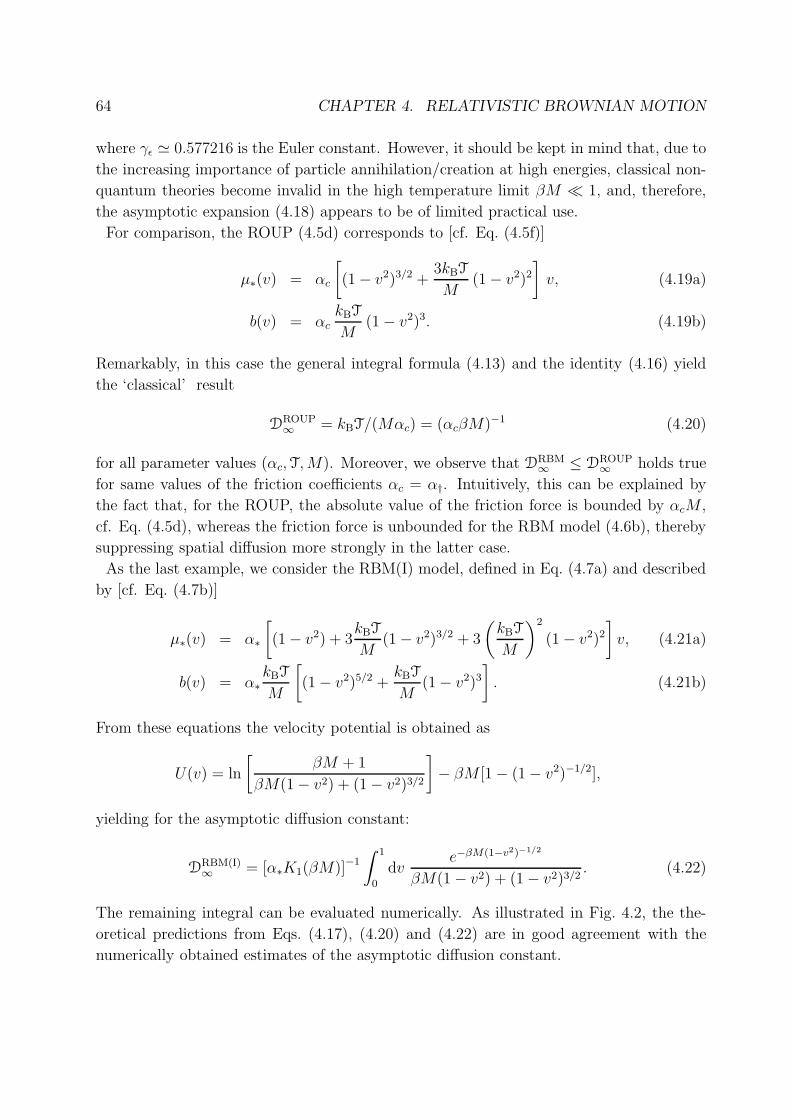
64 CHAPTER 4. RELATIVISTIC BROWNIAN MOTION
where γǫ ≃ 0.577216 is the Euler constant. However, it should be kept in mind that, due to
the increasing importance of particle annihilation/creation at high energies, classical non-
quantum theories become invalid in the high temperature limit βM ≪ 1, and, therefore,
the asymptotic expansion (4.18) appears to be of limited practical use.
For comparison, the ROUP (4.5d) corresponds to [cf. Eq. (4.5f)]
µ∗(v) = αc
[
(1 − v2)3/2 +3kBT
M(1 − v2)2
]
v, (4.19a)
b(v) = αckBT
M(1 − v2)3. (4.19b)
Remarkably, in this case the general integral formula (4.13) and the identity (4.16) yield
the ‘classical’ result
DROUP∞ = kBT/(Mαc) = (αcβM)−1 (4.20)
for all parameter values (αc,T,M). Moreover, we observe that DRBM∞ ≤ DROUP
∞ holds true
for same values of the friction coefficients αc = α†. Intuitively, this can be explained by
the fact that, for the ROUP, the absolute value of the friction force is bounded by αcM ,
cf. Eq. (4.5d), whereas the friction force is unbounded for the RBM model (4.6b), thereby
suppressing spatial diffusion more strongly in the latter case.
As the last example, we consider the RBM(I) model, defined in Eq. (4.7a) and described
by [cf. Eq. (4.7b)]
µ∗(v) = α∗
[
(1 − v2) + 3kBT
M(1 − v2)3/2 + 3
(
kBT
M
)2
(1 − v2)2
]
v, (4.21a)
b(v) = α∗kBT
M
[
(1 − v2)5/2 +kBT
M(1 − v2)3
]
. (4.21b)
From these equations the velocity potential is obtained as
U(v) = ln
[
βM + 1
βM(1 − v2) + (1 − v2)3/2
]
− βM [1 − (1 − v2)−1/2],
yielding for the asymptotic diffusion constant:
DRBM(I)∞ = [α∗K1(βM)]−1
∫ 1
0
dve−βM(1−v2)−1/2
βM(1 − v2) + (1 − v2)3/2. (4.22)
The remaining integral can be evaluated numerically. As illustrated in Fig. 4.2, the the-
oretical predictions from Eqs. (4.17), (4.20) and (4.22) are in good agreement with the
numerically obtained estimates of the asymptotic diffusion constant.
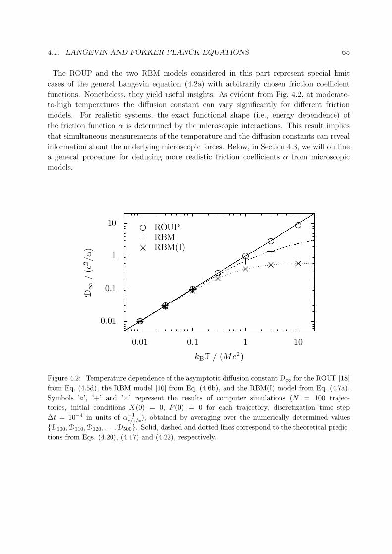
4.1. LANGEVIN AND FOKKER-PLANCK EQUATIONS 65
The ROUP and the two RBM models considered in this part represent special limit
cases of the general Langevin equation (4.2a) with arbitrarily chosen friction coefficient
functions. Nonetheless, they yield useful insights: As evident from Fig. 4.2, at moderate-
to-high temperatures the diffusion constant can vary significantly for different friction
models. For realistic systems, the exact functional shape (i.e., energy dependence) of
the friction function α is determined by the microscopic interactions. This result implies
that simultaneous measurements of the temperature and the diffusion constants can reveal
information about the underlying microscopic forces. Below, in Section 4.3, we will outline
a general procedure for deducing more realistic friction coefficients α from microscopic
models.
0.01
0.1
1
10
D∞/
(c2/α
)
0.01 0.1 1 10
kBT / (Mc2)
ROUPRBMRBM(I)
Figure 4.2: Temperature dependence of the asymptotic diffusion constant D∞ for the ROUP [18]
from Eq. (4.5d), the RBM model [10] from Eq. (4.6b), and the RBM(I) model from Eq. (4.7a).
Symbols ’◦’, ’+’ and ’×’ represent the results of computer simulations (N = 100 trajec-
tories, initial conditions X(0) = 0, P (0) = 0 for each trajectory, discretization time step
∆t = 10−4 in units of α−1c/†/∗), obtained by averaging over the numerically determined values
{D100,D110,D120, . . . ,D500}. Solid, dashed and dotted lines correspond to the theoretical predic-
tions from Eqs. (4.20), (4.17) and (4.22), respectively.
66 CHAPTER 4. RELATIVISTIC BROWNIAN MOTION
4.2 Moving observer
Thus far we have focussed on Langevin equations that describe the random motion of a
relativistic Brownian particle in the lab frame, defined as the rest frame of the heat bath.
In this part we would like to address the following question: Assuming that a Langevin
equation of the type (4.2a) holds in the lab frame – how does the corresponding process
look from the viewpoint of a moving observer?
To clarify this for the case of one spatial dimension (1D) we start from the Langevin
equations in the bath frame Σ,
dX(t) = (P/P 0) dt, (4.23a)
dP (t) = −α(P )P dt + [2D(P )]1/2 • dB(t), (4.23b)
and demand that α and D satisfy the relativistic Einstein relation βD(p) = α(p)E(p) with
E(P ) = (M2 + P 2)1/2 = P 0. Then, upon multiplying by p0 = (M2 +p2)1/2, the FPE (4.2c)
for the associated PDF f(t, x, p) can be written in the form(
p0 ∂
∂t+ p
∂
∂x
)
f = p0 ∂
∂p
[
α(p) p f +D(p)∂
∂pf
]
. (4.24)
As before, we will assume deterministic initial conditions X(0) = x0, P (0) =
p0 for the stochastic process (4.23), corresponding to a localized initial distribution
f(0, x, p) = δ(x− x0) δ(p− p0) in Σ.
In order to characterize the process (4.23) from the viewpoint of a moving inertial
frame Σ′, one can proceed as follows: According to van Kampen [138], the one-particle
phase space PDF f transforms as a Lorentz scalar, i.e., we have
f ′(t′, x′, p′) = f(t(t′, x′), x(t′, x′), p(p′)), (4.25a)
and, conversely,
f(t, x, p) = f ′(t′(t, x), x′(t, x), p′(p)), (4.25b)
where (t′, x′, p′) and (t, x, p) are related by the Lorentz transformations
(
t′
x′
)
= γ(w)
(
t− wx
−wt+ x
)
,
(
p′0
p′
)
= γ(w)
(
p0 − wp
−wp0 + p
)
, (4.26a)
(
t
x
)
= γ(w)
(
t′ + wx′
wt′ + x′
)
,
(
p0
p
)
= γ(w)
(
p′0 + wp′
wp′0 + p′
)
, (4.26b)
with w denoting the velocity of Σ′ relative to Σ, γ(w) = (1−w2)−1/2 and p′0 = (M2+p′2)1/2.
Thus, in order to find f ′, one merely needs to solve the Fokker-Planck equation (4.24) in
the lab frame Σ and, subsequently, insert the solution into Eq. (4.25a).
4.2. MOVING OBSERVER 67
4.2.1 Fokker-Planck and Langevin equations
On the other hand, it is also interesting to derive an explicit evolution equation for
f ′(t′, x′, p′) by starting from the lab frame FPE (4.24). To this end, we note that the
lhs. of Eq. (4.24) can be transformed as12
(
p0 ∂
∂t+ p
∂
∂x
)
f = pα∂α f = p′β ∂′β f′ =
(
p′0∂
∂t′+ p′
∂
∂x′
)
f ′, (4.27)
where (∂α) := (∂/∂t, ∂/∂x) and (pα) := (p0, p). The rhs. of Eq. (4.24) may be rewritten
in terms of the primed quantities as
p0 ∂
∂p
[
α(p) p f +D(p)∂
∂pf
]
= p0∂p′
∂p
∂
∂p′
[
α(p(p′)) p(p′) f ′ +D(p(p′))∂p′
∂p
∂
∂p′f ′
]
,
(4.28a)
where, by virtue of Eqs. (4.26), we have in the 1D case
p(p′) = γ(w) (wp′0
+ p′),∂p′
∂p=
p′0
γ(w) (p′0 + wp′)=p′0
p0. (4.28b)
Defining
α′(p′) := α(p(p′)), D′(p′) := D(p(p′)), (4.28c)
and combining Eqs. (4.27) and (4.28), we thus find the following FPE for the moving
observer
p′β ∂′β f′ = p′0
∂
∂p′
[
α′(p′) γ(w) (wp′0
+ p′) f ′ +D′(p′) p′0
γ(w) (p′0 + wp′)
∂
∂p′f ′
]
. (4.29)
Finally, upon dividing by p′0, this may be cast in the more familiar Fokker-Planck form(
∂
∂t′+p′
p′0∂
∂x′
)
f ′ =∂
∂p′
[
α′(p′) γ(w) (wp′0
+ p′) f ′ +D′(p′) p′0
γ(w) (p′0 + wp′)
∂
∂p′f ′
]
. (4.30)
The post-point SDE corresponding to this FPE reads
dX ′(t′) = (P ′/P ′0) dt′, (4.31a)
dP ′(t′) = A(P ′;w) dt′ + C(P ′;w) • dB′(t′), (4.31b)
where B′(t′) now is a standard Wiener process with time parameter t′, and
A(p′;w) := −α′(p′) γ(w) (wp′0
+ p′), C(p′;w) :=
[
2D′(p′) p′0
γ(w) (p′0 + wp′)
]1/2
. (4.31c)
Equations (4.31) describe how the stochastic process (4.23) would look like from the stand-
point of a moving observer who sees the lab frame flying past at velocity −w. In particular,
for w = 0 Eqs. (4.31) coincide with the lab frame Langevin equation (4.23).13
12Here and below, we use the sum convention aαbα :=∑
α aαbα.
13We note that, in general, a t-simultaneously specified initial condition f(0,x,p) in the lab frame Σ
corresponds to a non-simultaneous initial condition in the moving frame Σ′ – unless one considers a strictly
68 CHAPTER 4. RELATIVISTIC BROWNIAN MOTION
4.2.2 Covariant formulation
The FPE (4.30) describes the process (4.23) in the moving frame, but is not yet written a
manifestly covariant form. In order to achieve this, we return to Eq. (4.29). Dropping the
primes and writing f(t, x, p;w), α(p0, p;w) and D(p0, p;w) instead, Eq. (4.29) becomes
pβ ∂β f = p0 ∂
∂p
[
α(p0, p;w) γ(w) (wp0 + p) f +D(p0, p;w)
γ(w) (p0 + wp)p0 ∂
∂pf
]
, (4.32)
with (pα) = (p0, p) denoting the contravariant momentum four-vector of the Brownian
particle and p0 = (M2 + p2)1/2. If an observer moves at velocity w relative to the lab
frame, defined as mean rest frame of the bath, then from her point of view the heat bath
moves at velocity −w. Introducing the contravariant mean velocity four-vector of the heat
bath by (Uα) := γ(w)(1,−w), we may simplify
γ(w) (p0 + wp) = −Uαpα. (4.33)
Since f, α and D transform as Lorentz scalars and because of p0∂/∂p = p′0∂/∂p′ in the 1D
case, we can already see that the rhs. of Eq. (4.32) is indeed Lorentz invariant. However,
to obtain a manifestly covariant form of Eq. (4.32), we consider the momentum derivative
of some Lorentz scalar function g(p) = G(p0(p), p) and note that
p0 ∂
∂pg(p) = p0
{
∂
∂pG(p0, p) +
[
∂
∂p0G(p0, p)
]
∂p0
∂p
}
= p0
{
∂
∂pG(p0, p) +
[
∂
∂p0G(p0, p)
]
p
p0
}
= p0 ∂
∂pG(p0, p) + p
∂
∂p0G(p0, p)
= −p0∂
∂pG(p0, p) + p
∂
∂p0G(p0, p)
= −εαβpα∂
∂pβG(p0, p). (4.34)
Here, (pα) = (p0, p) = (−p0, p) is the covariant momentum four-vector and the total
antisymmetric Levi-Cevita tensor εαβ is defined by14
ε01 = −ε10 = 1 , ε00 = ε11 = 0.
Thus, by means of Eq. (4.34), Eq. (4.32) can be written in the Lorentz invariant form
pβ ∂β f = εαβpα∂
∂pβ
[
α(pν;w)Uηpη f +D(pµ;w)
−Uκpκ
εγδpγ∂
∂pδf
]
. (4.35)
localized initial condition of the form f(0,x,p) = δ(x − x0)δ(p − p0).14For a Lorentz boost of the form (3.6), one finds that ε′αβ = Λα
γΛβδε
γδ = εγδ, i.e., the Levi-Cevita ten-
sor is numerically invariant under Lorentz transformations with determinant +1. For a general discussion
of the properties of Levi-Cevita tensors we refer to Section 5.5 of Sexl and Urbantke [8].
4.3. RELATIVISTIC BINARY COLLISION MODEL 69
4.3 Relativistic binary collision model
The two preceding sections have focussed on general aspects of relativistic Langevin and
Fokker-Planck equations. Similar to the nonrelativistic case, relativistic SDEs present
a useful tool for analytical and numerical studies of relaxation processes in relativistic
systems. Stochastic models of this type provide a simplified picture of the underlying
microscopic dynamics. In order for the Langevin approach to be successful, one must
know in advance which friction coefficient function α(P ) and noise amplitude D(P ) are
appropriate for the system under consideration. In the remainder of this section, we
will discuss a systematic procedure for obtaining friction coefficients and noise amplitudes
from a simple microscopic interaction model [13]. The latter can be viewed as the direct
relativistic generalization of the elastic binary collision model from Section 2.2.2. More
precisely, we consider a 1D system consisting of a heavy Brownian particle (mass M)
which is embedded into a heat bath of smaller particles (mass m ≪ M , total number
N ≫ 1). Our model assumes that the stochastic motion of a Brownian particle arises
due to frequent elastic interactions with the surrounding heat bath particles. Similar to
Section 2.2.2, we are interested in finding the ‘best’ approximation of the ‘exact’ dynamics
within the class of SDEs defined by Eq. (4.2a).
Relativistic collision kinematics To begin with, we consider a single collision of the
Brownian particle (momentum P , energy E) with a heat bath particle (momentum p,
energy ǫ). The relativistic energy, momentum and velocity of the two particles before the
collision are given by
P = MV γ(V ), E(P ) =(
M2 + P 2)1/2
, (4.36a)
p = mv γ(v), ǫ(p) =(
m2 + p2)1/2
. (4.36b)
where γ(v) ≡ (1 − v2)−1/2
. Considering elastic interactions, the collision kinematics is
governed by the relativistic mass-energy-momentum conservation laws
M = M, m = m, E + ǫ = E + ǫ, P + p = P + p, (4.37)
where hat-symbols refer to the state after the collision. Inserting Eqs. (4.36) into the
conservation laws (4.37), and solving for the momentum of Brownian particle after the
collision, P , we obtain [13]
P = γ(u)2 [2uE − (1 + u2)P ], (4.38a)
where the collision-invariant center-of-mass velocity u is given by
u(p, P ) =P + p
E + ǫ. (4.38b)
70 CHAPTER 4. RELATIVISTIC BROWNIAN MOTION
Accordingly, the momentum change
∆Pr := P − P
of the Brownian particle in a single collision with the heat bath particle ‘r’ is given by
∆Pr = −2γ(ur)2 ǫrE + ǫr
P + 2γ(ur)2 E
E + ǫrpr, (4.39)
where ur := u(pr, P ) and ǫr := ǫ(pr). In the non-relativistic limit case, where u2r ≪ 1,
E ≃M and ǫr ≃ m, Eq. (4.39) reduces to Eq. (2.43).
Furthermore, by making the same assumptions as in Section 2.2.2, we find that the
momentum change δP (t) := P (t+ δt)−P (t) of the Brownian particle during a small-but-
sufficiently-long time interval [t, t+ δt] can be approximated by
δP (t) ≈N
∑
r=1
∆Pr Ir(t, δt)
≈ −2N
∑
r=1
γ(ur)2 ǫrE + ǫr
P (t) Ir(t, δt) + 2N
∑
r=1
γ(ur)2 E
E + ǫrpr Ir(t, δt). (4.40a)
Formally, the collision indicator Ir(t, τ) is again given by [cf. Eq. (2.48a)]
Ir(t, δt) ≈ δt
2|vr − V | δ(xr −X), (4.40b)
but now we have to use the relativistic velocities
V = P/(M2 + P 2)1/2 , vr = pr/(M2 + p2
r)1/2. (4.40c)
Equation (4.40a) is the relativistic counterpart of Eq. (2.48b). Heuristically, the first
term on the rhs. of Eq. (4.40a) can again be interpreted as ‘friction’, while the second
contribution may be viewed as ‘noise’.
Bath distribution and drift Similar to the nonrelativistic case, Eqs. (4.40) can be used
to calculate the statistical moments 〈[δP (t)]j〉b of the momentum increments – provided
one specifies the phase space distribution of the heat bath particles. We will assume here
that the heat bath is in a thermal equilibrium state, so that the one-particle phase space
PDF is given by a spatially homogeneous Juttner function
f 1b (xr, pr) = (ZJL)−1 exp
[
−(m2 + p2r)
1/2
kBT
]
, (4.41a)
where L is the 1D volume, T = (βkB)−1 the temperature, and
ZJ = 2mK1(βm), (4.41b)
4.3. RELATIVISTIC BINARY COLLISION MODEL 71
with K1(z) denoting the modified Bessel function. With regard to our subsequent discus-
sion, we are interested in calculating the mean drift force g, defined by15
g(P ) :=
⟨
δP (t)
δt
⟩
b
. (4.42)
Inserting δP (t) from Eq. (4.40a), we find
g(P ) = −nb
⟨
2γ(ur)2 ǫrE + ǫr
LIrδt
⟩
b
P + nb
⟨
2γ(ur)2 E
E + ǫrprLIrδt
⟩
b
, (4.43)
where nb = N/L is the number density of the bath particles. In order to determine g(P ),
we note that for some arbitrary function G(p, P ), we have
⟨
G(pr, P )LIr(t, δt)
δt
⟩
b
= (2ZJ)−1
∫ ∞
−∞
dp G(pr, P ) exp
[
−(m2 + p2r)
1/2
kBT
]
×∣
∣
∣
∣
pr
(m2 + p2r)1/2
− P
(M2 + P 2)1/2
∣
∣
∣
∣
. (4.44)
The first term on the rhs. of Eq. (4.43) involves the function
G1(p, P ) := 2γ(ur)2 ǫ(p)
E(P ) + ǫ(p), (4.45a)
and the second term
G2(p, P ) := 2γ(ur)2 E(P )
E(P ) + ǫ(p)p. (4.45b)
Unfortunately, it is very difficult or perhaps even impossible to analytically evaluate the
integral (4.44) for the functions G1/2. Figure 4.3 depicts the mean drift force g(P ), obtained
by numerically integrating the formula (4.44) for different values of P .
Langevin approximation We conclude this section by discussing how one could, in
principle, approximate Eqs. (4.40) by a nonlinear SDE of the form (4.2a), i.e., by
dP (t) = −α(P )P dt+ [2D(P )]1/2 • dB(t). (4.46)
The considerations from Chapter 3 imply that the stationary momentum distribution of
the Brownian particle in the binary collision model is given by the Juttner function
φJ(p) = Z−1J exp[−β(p2 +M2)1/2] , ZJ = 2M K1(βM). (4.47)
15In principle, higher moments⟨
[δP (t)]j⟩
b, j > 1, can be calculated in a similar manner, but then one
has to specify the j-particle heat bath PDF f jb.
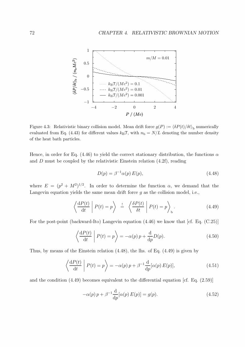
72 CHAPTER 4. RELATIVISTIC BROWNIAN MOTION
−1
−0.5
0
0.5
1
〈δP/δt〉
b/
(nbMc2
)〈δP/δt〉
b/
(nbMc2
)
−4 −2 0 2 4
P / (Mc)P / (Mc)
kBT/(Mc2) = 0.1
kBT/(Mc2) = 0.01
kBT/(Mc2) = 0.001
m/M = 0.01
Figure 4.3: Relativistic binary collision model. Mean drift force g(P ) := 〈δP (t)/δt〉b numerically
evaluated from Eq. (4.43) for different values kBT, with nb = N/L denoting the number density
of the heat bath particles.
Hence, in order for Eq. (4.46) to yield the correct stationary distribution, the functions α
and D must be coupled by the relativistic Einstein relation (4.2f), reading
D(p) = β−1α(p)E(p), (4.48)
where E = (p2 + M2)1/2. In order to determine the function α, we demand that the
Langevin equation yields the same mean drift force g as the collision model, i.e.,
⟨
dP (t)
dt
∣
∣
∣
∣
P (t) = p
⟩
!=
⟨
δP (t)
δt
∣
∣
∣
∣
P (t) = p
⟩
b
. (4.49)
For the post-point (backward-Ito) Langevin equation (4.46) we know that [cf. Eq. (C.25)]
⟨
dP (t)
dt
∣
∣
∣
∣
P (t) = p
⟩
= −α(p) p+d
dpD(p). (4.50)
Thus, by means of the Einstein relation (4.48), the lhs. of Eq. (4.49) is given by
⟨
dP (t)
dt
∣
∣
∣
∣
P (t) = p
⟩
= −α(p) p+ β−1 d
dp[α(p)E(p)], (4.51)
and the condition (4.49) becomes equivalent to the differential equation [cf. Eq. (2.59)]
−α(p) p+ β−1 d
dp[α(p)E(p)] = g(p). (4.52)
4.3. RELATIVISTIC BINARY COLLISION MODEL 73
In the case of the collision model, where the function g(p) is not exactly known, one could,
e.g., try to fit g(p) by a simple analytic expression and, subsequently, use this approximation
in Eq. (4.52).16
16Alternatively, one can also try to derive a Fokker-Planck equation from, e.g., a relativistic Boltzmann
equation [278,294].

74 CHAPTER 4. RELATIVISTIC BROWNIAN MOTION

Chapter 5
Non-Markovian relativistic diffusion
The preceding chapter was dedicated to relativistic Brownian motions in phase space. In
the remainder we will discuss relativistic diffusion models in Minkowski space-time, i.e.,
continuous relativistic processes that do not explicitly depend on the momentum coor-
dinate. On the one hand, such space-time processes may be constructed, e.g., from a
Brownian motion processes in phase space by integrating out the momentum coordinates.
As a result of this averaging procedure, the reduced process for the position coordinate will
be non-Markovian. Alternatively, one can try to derive or postulate a relativistic diffusion
equation and/or diffusion propagators by means of microscopic models [140, 375,377,381]
or plausibility considerations [15]. Regardless of the approach adopted, in order to comply
with the principles of special relativity, the resulting space-time process must be non-
Markovian, as rigorously proven by Dudley (Theorem 11.3 in [341]) and Hakim (Propo-
sition 2 in [346]). Put differently, any relativistic generalization of the nonrelativistic
diffusion equation (1.1) with constant coefficients should be of at least second order in the
time coordinate.
The construction and analysis of relativistic diffusion models in Minkowski space-time
poses an interesting problem in its own right. In addition, the investigation of these
processes becomes relevant in view of potential analogies with relativistic quantum the-
ory [329, 398], similar to the analogy between Schrodinger’s equation and the diffusion
equation (1.1) in the nonrelativistic case [474,475]. The present section intends to provide
an overview over classical relativistic diffusion models that have been discussed in the lit-
erature [15,329,345,375–377,381,390–392,395,396]. For this purpose, we first recall basic
properties of the Wiener (Gaussian) process, which constitutes the standard paradigm for
nonrelativistic diffusions in position space (Section 5.1). Subsequently, relativistic general-
izations of the nonrelativistic diffusion equation (1.1) and/or the nonrelativistic Gaussian
diffusion propagator will be discussed [15].
75
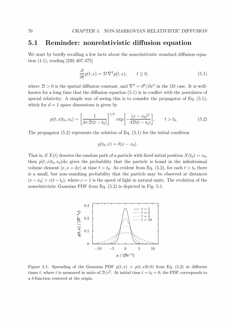
76 CHAPTER 5. NON-MARKOVIAN RELATIVISTIC DIFFUSION
5.1 Reminder: nonrelativistic diffusion equation
We start by briefly recalling a few facts about the nonrelativistic standard diffusion equa-
tion (1.1), reading [220,407,475]
∂
∂t(t, x) = D∇2(t, x), t ≥ 0, (5.1)
where D > 0 is the spatial diffusion constant, and ∇2 = ∂2/∂x2 in the 1D case. It is well-
known for a long time that the diffusion equation (5.1) is in conflict with the postulates of
special relativity. A simple way of seeing this is to consider the propagator of Eq. (5.1),
which for d = 1 space dimensions is given by
p(t, x|t0, x0) =
[
1
4πD(t− t0)
]1/2
exp
[
− (x− x0)2
4D(t− t0)
]
, t > t0. (5.2)
The propagator (5.2) represents the solution of Eq. (5.1) for the initial condition
(t0, x) = δ(x− x0).
That is, if X(t) denotes the random path of a particle with fixed initial position X(t0) = x0,
then p(t, x|t0, x0)dx gives the probability that the particle is found in the infinitesimal
volume element [x, x+ dx] at time t > t0. As evident from Eq. (5.2), for each t > t0 there
is a small, but non-vanishing probability that the particle may be observed at distances
|x−x0| > c(t− t0), where c = 1 is the speed of light in natural units. The evolution of the
nonrelativistic Gaussian PDF from Eq. (5.2) is depicted in Fig. 5.1.
0
0.1
0.2
0.3
(t,x
)/
(D−
1c)
(t,x
)/
(D−
1c)
−10 −5 0 5 10
x / (Dc−1)x / (Dc−1)
t = 1t = 2t = 4t = 10
Figure 5.1: Spreading of the Gaussian PDF (t, x) = p(t, x|0, 0) from Eq. (5.2) at different
times t, where t is measured in units of D/c2. At initial time t = t0 = 0, the PDF corresponds to
a δ-function centered at the origin.
5.1. REMINDER: NONRELATIVISTIC DIFFUSION EQUATION 77
We next summarize basic properties of Eqs. (5.1) and (5.2): Equation (5.1) is a linear
parabolic partial differential equation. Due to the linearity, more general solutions may
be constructed by superpositioning, i.e., by integrating the solution (5.2) over some given
initial PDF 0(x0). Equation (5.1) describes a Markov process which means that the
transition PDF (5.2) satisfies the Chapman-Kolmogoroff criterion
p(t, x|t0, x0) =
∫
R
dx1 p(t, x|t1, x1) p(t1, x1|t0, x0) (5.3)
for all t1 ∈ (t0, t). The corresponding diffusion process X(t) can be characterized in terms
of the following SDE:
dX(t) = (2D)1/2 ∗ dB(t), X(t0) = x0, (5.4)
where B(t) is a standard Wiener process as defined in Section 2.1.1. Formally, Eq. (5.4)
may be obtained from the Langevin equation (2.3b) of the classical Ornstein-Uhlenbeck
process as follows: First we rewrite Eq. (2.3b) as
dV (t)
Mα= −V dt +
(
2D
M2α2
)1/2
∗ dB(t). (5.5)
Upon letting (Mα) → ∞ and D → ∞ such that D = D/(αM)2 remains constant, the
lhs. of Eq. (5.5) should become negligible. Then, by making use of dX = V dt, Eq. (5.4) is
recovered. This limiting procedure defines the so-called overdamped regime of the Ornstein-
Uhlenbeck process. The mean square displacement of the overdamped process (5.4) is given
by [220]
⟨
[X(t) −X(t0)]2⟩
:=
∫
dx (x− x0)2 p(t, x|t0, x0)
= 2D (t− t0), (5.6)
qualitatively similar to that of classical Ornstein-Uhlenbeck process; cf. Eq. (2.8). Finally,
we note that the solution of Eq. (5.1) with initial condition
(t0, x) ≡ 0(x), (5.7)
can be expressed in the Feynman-Kac form [64,66]
(t, x) =⟨
0
(
x+ (2D)1/2B(t))⟩
(5.8)
where 〈 · 〉 indicates an average with respect to the standard Wiener process B(t) with
initial condition B(t0) = 0. Equation (5.8) yields an efficient Monte-Carlo simulation
scheme for computing the solutions of the diffusion equation (5.1).
78 CHAPTER 5. NON-MARKOVIAN RELATIVISTIC DIFFUSION
5.2 Telegraph equation
The problem of constructing continuous diffusion models which, in contrast to Eqs. (5.1)
and (5.2), avoid superluminal velocities, has attracted considerable interest over the past
years [15, 329, 345, 375–377, 381, 390–392, 395, 396]. Nonetheless, it seems fair to say that
a commonly accepted solution is still outstanding. Apart from the profound theoretical
challenge of developing a consistent relativistic diffusion theory, there exist several practical
applications including, e.g., the analysis of data from high energy collision experiments [393,
394,406] or the diffusion of light through turbid media [383,476,477] and foams [384–386].
In this context, a frequently considered alternative to Eq. (5.1) is given by the telegraph
equation [375,377,380,388–391,393–396]
(
τv∂2
∂t2+∂
∂t
)
(t, x) = D∇2(t, x). (5.9)
Here, D > 0 plays again the role of a diffusion constant, while τv > 0 is an additional
relaxation time parameter. Similar to Eq. (5.1), the telegraph equation (5.9) refers to a
special frame where the background medium, causing the random motion of the diffusing
test particle, is at rest (on average). The ‘nonrelativistic limit’ corresponds to letting τv → 0
in Eq. (5.9), which leads back to Eq. (5.1). For τv > 0, Eq. (5.9) is a linear hyperbolic
partial differential equation. Because of the second order time derivative in Eq. (5.9), one
now also has to specify the first order time derivative of the initial distribution at time t0.
Considering particular initial conditions
(t0, x) = δ(x− x0),∂
∂t(t0, x) ≡ 0, (5.10)
one finds that the corresponding solution of Eq. (5.9) is given by [375,377]
p(t, x|t0, x0) =e−(t−t0)/(2τv)
2
{
δ[|x− x0| − v(t− t0)] +
Θ(ξ2)
2τvv
[
I0(ξ) +t
2τv
I1(ξ)
ξ
]}
. (5.11a)
Here, we have abbreviated
ξ :=1
2
[
(
t− t0τv
)2
−(
x− x0
τvv
)2]1/2
, v := (D/τv)1/2, (5.11b)
and the modified Bessel functions of the first kind, Iν(z), are defined by
Iν(z) :=
∞∑
k=0
1
Γ(k + ν + 1) k!
(z
2
)2k+ν
5.2. TELEGRAPH EQUATION 79
with Γ(z) denoting the Euler gamma function. According to our knowledge, the solu-
tion (5.11) was first obtained by Goldstein in 1938/1939. Actually, Goldstein derived the
result (5.11) by considering the continuum limit of a persistent random walk model [379];
subsequently, he proved that this function satisfies the telegraph equation (5.9), cf. Sec-
tion 8 of his paper [375].
The propagator (5.11) is characterized by two salient features:
a) As evident from the δ-function term, the solution exhibits two singular diffusion
fronts traveling at absolute velocity v := (D/τv)1/2 to the left and right, respectively;
b) due to the appearance of the Heaviside Θ-function, the solution is non-zero only
within the region |x − x0| ≤ v(t − t0), i.e., upon fixing τv such that v = c = 1 the
solution vanishes outside the light cone.
Thus, in contrast to the nonrelativistic propagator (5.2), Eqs. (5.11) define a relativisti-
cally acceptable diffusion model. Because of the second order time derivative, the telegraph
equation (5.9) describes a non-Markovian process, in accordance with the aforementioned
theorems of Dudley [341] and Hakim [346]. The non-Markovian character of the propa-
gator (5.11) can also be proven directly by verifying that this solution does not fulfill the
condition (5.3).
The linearity of Eq. (5.9) implies that more general solutions can be obtained by in-
tegrating the propagator (5.11) over some given initial distribution 0(x0). In principle,
one may also construct other classes of solutions with ∂(t0, x)/∂t 6≡ 0, e.g., by applying
a Laplace-Fourier transformation [377, 478, 479] to Eq. (5.9). We note, however, that in
order for the solution (t, x) to remain normalized at all times t > t0, it is required that∫ +∞
−∞
dx∂
∂t(t0, x) ≡ 0, (5.12a)
and
∂
∂x(t,±∞) ≡ 0. (5.12b)
In the case of Eq. (5.10), these conditions are automatically satisfied. Various solutions and
extensions of the telegraph equation (5.9), including different types of boundary conditions,
additional external sources, etc., have been discussed, e.g., by Goldstein [375], Masoliver
et al. [478, 479], Foong and Kanno [480], Renardy [481], and Dorogovtsev [482].
Similar to the nonrelativistic diffusion equation (5.1), the telegraph equation (5.9) may
be derived and/or motivated in many different ways. A detailed overview is given by
Masoliver and Weiss [377], who discuss four different possibilities of deducing Eq. (5.9)
from underlying models; see also Koide [395, 396]. During the past decades, the telegraph
equation (5.9) has been used to describe a number of different phenomena. The applications
include:
80 CHAPTER 5. NON-MARKOVIAN RELATIVISTIC DIFFUSION
• Transmission of electrical signals. According to Masoliver and Weiss (5.9), the earli-
est derivation of the telegraph equation is based on a paper by William Thomson [483]
(who later became Lord Kelvin), published in 1855. He considered the problem of
how to transmit electrical signals without distortion, a question closely related to the
design of the first transatlantic cable.
• Continuum models of persistent diffusion. It seems that the concept of persistent
diffusion was first proposed in 1917/1922 by Furth [378, 379] who aimed at describ-
ing the random motion of biological objects. Independently, a similar approach was
suggested by Taylor [380] in an attempt to treat turbulent diffusion [376]. Furth
and Taylor considered discrete models, assuming that a particle moves with con-
stant absolute velocity between neighboring lattice points. At each lattice point,
the particle is either back-scattered or transmitted, with the transmission probabil-
ity being larger than the back-scattering probability (persistence). A few decades
later, in 1950, Goldstein [375] demonstrated for the 1D case1 that, for a suitable
choice of the transition probabilities, the continuum limit of this model leads to
the telegraph equation. Hence, in contrast to the ordinary diffusion equation (5.1),
the telegraph equation (5.9) relies on asymmetric transition probabilities, causing
the non-vanishing probability concentration at the diffusion fronts. In more recent
years, persistent diffusion models have been employed to describe the propagation of
photons in thin slabs and foams [382–386].
• Heat transport and propagation of heat waves. In this case, the function (t, x) in
Eq. (5.9) is interpreted as a temperature field and the normalization condition is
usually dropped. For a detailed account of the vast literature on heat waves we refer
to the review article of Joseph and Preziosi [388, 389].
• High energy ion collision experiments. In recent years, the telegraph equation has
been used to estimate the dissipation of net charge fluctuations, which may obliterate
signals of QCD phase transitions in nuclear collisions [393, 394]. In this context,
however, the coordinate x in Eq. (5.9) is interpreted as a rapidity variable.
Another interesting aspect of the telegraph equation is elucidated in a paper by Kac [376].
He observed that the solutions of Eq. (5.9) with initial conditions
(t0, x) ≡ 0(x),∂
∂t(t0, x) ≡ 0, (5.13)
1Boguna et al. [381] discuss persistent random walks in higher space dimensions.
5.2. TELEGRAPH EQUATION 81
may be expressed in the form2
(t, x) =1
2
⟨
0
(
x− v
∫ t
t0
ds (−1)N(s)
)⟩
+
1
2
⟨
0
(
x + v
∫ t
t0
ds (−1)N(s)
)⟩
, (5.14)
where v = (D/τv)1/2, and 〈 · 〉 indicates an average with respect to the τv-parameterized
Poisson process N(t); i.e., for any given time t > t0 we have
Prob{N(t) = k} =e−(t−t0)/(2τv)
k!
(
t− t02τv
)k
, k = 0, 1, 2, . . . ; (5.15a)
and for any finite sequence t0 < t1 < . . . < tn the increments
N(t1) −N(t0), N(t2) −N(t1), . . . , N(tn) −N(tn−1) (5.15b)
are independent. Equation (5.14) is the direct counterpart of Feynman-Kac formula (5.8).
Equations (5.14) and (5.15) together provide a very efficient Monte-Carlo simulation
scheme for computing solutions of the telegraph equation (5.9). Moreover, the Poisson
path integral representation (5.14) discloses an interesting correspondence between the
free-particle Dirac equation [397] and the telegraph equation (5.9), which was first pointed
out by Gaveau et al. [398] in 1984: The solutions of both equations may be linked by means
of an analytic continuation. This connection is similar to the relation between the diffusion
equation (5.1) and the free particle Schrodinger equation in the nonrelativistic case.3 The
crucial difference is given by the fact that the measures of the functional integration refer
to different underlying processes, respectively.
However, the telegraph equation (5.9) is not the only possible relativistic generalization of
the nonrelativistic diffusion equation (1.1) and, recently, there has been some controversy
about its applicability and validity [390–392]. An early critical discussion of Eq. (5.9) in
the context of relativistic heat transport was given by van Kampen [140] in 1970. Starting
from a simple microscopic model, consisting of a cloud of material particles that exchange
electromagnetic radiation, van Kampen derived an integral equation for the temperature
of the particles as function of time and space. He then showed how the telegraph equa-
tion (5.9) can be recovered as an approximation to the more precise integral equation, but
that the validity of this approximation breaks down in the vicinity of the diffusion fronts.
2The result (5.14) may be generalized to an arbitrary number of space dimensions; cf. pp. 500 in Kac’s
paper [376].3For further reading about path integral representations of the Dirac propagator we refer to the papers of
Ichinose [399,400], Jacobson and Schulman [401], Barut and Duru [402], and Gaveau and Schulman [403];
see also footnote 7 in Gaveau et al. [398] and problem 2-6, pp. 34-36 in Feynman and Hibbs [404].
82 CHAPTER 5. NON-MARKOVIAN RELATIVISTIC DIFFUSION
Similarly, the singular diffusion fronts predicted by Eq. (5.11) represent a source of con-
cern if one wishes to adopt the telegraph equation (5.9) as a model for particle transport
in a random medium. While these singularities may be acceptable in the case of photon
diffusion [382–386], they seem unrealistic for massive particles, because such fronts would
imply that a finite fraction of particles carries a huge amount of kinetic energy (much
larger than mc2). In view of these shortcomings, it appears reasonable to explore other
constructions of relativistic diffusion processes [15, 405]. In the next part we will propose
a different approach [15] that may provide a viable alternative to the solutions of the
telegraph equation.
5.3 Relativistic diffusion propagator
In principle, one can distinguish two different routes towards constructing relativistic dif-
fusion processes: One can either try to find an acceptable relativistic diffusion equation,
or one can focus directly on the structure of the diffusion propagator. In the present part
we shall adopt the latter approach [15]. The basic idea is to rewrite the nonrelativis-
tic diffusion propagator (5.2) in such a form that its relativistic generalized follows in a
straightforward manner. This can be achieved be reexpressing Eq. (5.2) in terms of an
integral-over-actions.
For this purpose, we consider a nonrelativistic particle traveling from the event x0 =
(t0, x0) to x = (t, x). We assume that the particle can experience multiple scatterings on
its way, and that the velocity is approximately constant between two successive scattering
events. Then the total action (per mass) required along the path is given by
a(x|x0) =1
2
∫ t
t0
dt′ v(t′)2, (5.16)
where the velocity v(t′) is a piecewise constant function, satisfying
x = x0 +
∫ t
t0
dt′ v(t′). (5.17)
Clearly, the nonrelativistic action (5.16) becomes minimal for the deterministic (direct)
path, i.e., if the particle does not collide at all. In this case, it moves with constant
velocity v(t′) ≡ (x− x0)/(t− t0) for all t′ ∈ [t0, t], yielding the smallest possible action
value
a−(x|x0) =(x− x0)2
2(t− t0). (5.18)
On the other hand, to match the boundary conditions it is merely required that the mean
velocity equals (x − x0)/(t − t0). Consequently, in the nonrelativistic case, the absolute
5.3. RELATIVISTIC DIFFUSION PROPAGATOR 83
velocity of a particle may become arbitrarily large during some intermediate time inter-
val [t′, t′′] ⊂ [t0, t]. Hence, the largest possible action value is a+(x, x0) = +∞. These
considerations put us in the position to rewrite the Wiener propagator (5.2) as an integral-
over-actions:
p(x|x0) ∝∫ a+(x|x0)
a−(x|x0)
da exp
(
− a
2D
)
, (5.19a)
supplemented by the normalization condition
1 =
∫
dx p(x|x0). (5.19b)
The representation (5.19) may be generalized to the relativistic case in a straightforward
manner: One merely needs to insert the corresponding relativistic expressions into the
boundaries of the integral (5.19a). A commonly considered relativistic generalization of
Eq. (5.16), based on the particle’s proper time, reads [6]
a = −∫ t
t0
dt′[
1 − v(t′)2]1/2
. (5.20)
Analogous to the nonrelativistic case, the relativistic action (5.20) assumes its minimum
a− for the deterministic (direct) path from x0 to x, characterized by a constant velocity
v(t′) ≡ (x− x0)/(t− t0). One explicitly obtains
a−(x, x0) = −[
(t− t0)2 − (x− x0)2]1/2
, (5.21a)
i.e., a− is the negative Minkowski distance of the two space-time events x0 and x. The
maximum action value is realized for particles moving at light speed, yielding a+ = 0.
Hence, the transition PDF for the relativistic generalization of the Wiener process reads
p(x|x0) = N−1
{
exp
[
−a−(x, x0)
2D
]
− 1
}
, (5.21b)
if (x− x0)2 ≤ (t− t0)
2, and p(x|x0) ≡ 0 otherwise, with a− determined by Eq. (5.21a).
The relativistic diffusion process defined by Eqs. (5.21) is non-Markovian, i.e., it does not
fulfill Chapman-Kolmogoroff criterion (5.3). The functional form of the propagator (5.21b)
remains the same for higher space dimensions d > 1; the corresponding normalization
constants are given in the App. B. In contrast to the solution (5.11) of the telegraph
equation, the propagator (5.21b) vanishes continuously at the diffusion fronts. Figure 5.2
depicts the PDF (t, x) = p(t, x|0, 0) of the diffusion process (5.21) for the one-dimensional
case d = 1 at different times t. The corresponding mean square displacement is plotted in
Fig. 5.3 (dashed curve).
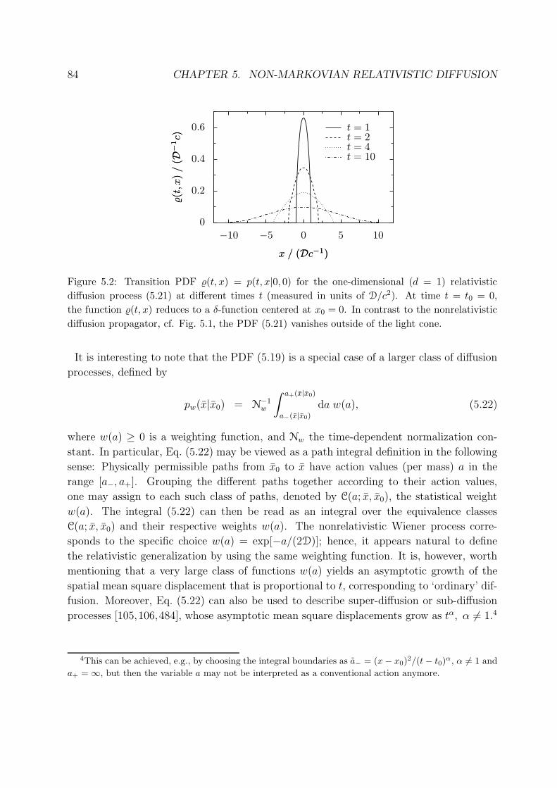
84 CHAPTER 5. NON-MARKOVIAN RELATIVISTIC DIFFUSION
0
0.2
0.4
0.6
(t,x
)/
(D−
1c)
(t,x
)/
(D−
1c)
−10 −5 0 5 10
x / (Dc−1)x / (Dc−1)
t = 1t = 2t = 4t = 10
Figure 5.2: Transition PDF (t, x) = p(t, x|0, 0) for the one-dimensional (d = 1) relativistic
diffusion process (5.21) at different times t (measured in units of D/c2). At time t = t0 = 0,
the function (t, x) reduces to a δ-function centered at x0 = 0. In contrast to the nonrelativistic
diffusion propagator, cf. Fig. 5.1, the PDF (5.21) vanishes outside of the light cone.
It is interesting to note that the PDF (5.19) is a special case of a larger class of diffusion
processes, defined by
pw(x|x0) = N−1w
∫ a+(x|x0)
a−(x|x0)
da w(a), (5.22)
where w(a) ≥ 0 is a weighting function, and Nw the time-dependent normalization con-
stant. In particular, Eq. (5.22) may be viewed as a path integral definition in the following
sense: Physically permissible paths from x0 to x have action values (per mass) a in the
range [a−, a+]. Grouping the different paths together according to their action values,
one may assign to each such class of paths, denoted by C(a; x, x0), the statistical weight
w(a). The integral (5.22) can then be read as an integral over the equivalence classes
C(a; x, x0) and their respective weights w(a). The nonrelativistic Wiener process corre-
sponds to the specific choice w(a) = exp[−a/(2D)]; hence, it appears natural to define
the relativistic generalization by using the same weighting function. It is, however, worth
mentioning that a very large class of functions w(a) yields an asymptotic growth of the
spatial mean square displacement that is proportional to t, corresponding to ‘ordinary’ dif-
fusion. Moreover, Eq. (5.22) can also be used to describe super-diffusion or sub-diffusion
processes [105,106,484], whose asymptotic mean square displacements grow as tα, α 6= 1.4
4This can be achieved, e.g., by choosing the integral boundaries as a− = (x− x0)2/(t− t0)α, α 6= 1 and
a+ = ∞, but then the variable a may not be interpreted as a conventional action anymore.
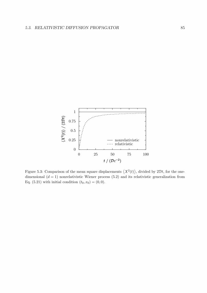
5.3. RELATIVISTIC DIFFUSION PROPAGATOR 85
0
0.25
0.5
0.75
1
〈X2(t
)〉/
(2Dt)
〈X2(t
)〉/
(2Dt)
0 25 50 75 100
t / (Dc−2)t / (Dc−2)
nonrelativisticrelativistic
Figure 5.3: Comparison of the mean square displacements⟨
X2(t)⟩
, divided by 2Dt, for the one-
dimensional (d = 1) nonrelativistic Wiener process (5.2) and its relativistic generalization from
Eq. (5.21) with initial condition (t0, x0) = (0, 0).

86 CHAPTER 5. NON-MARKOVIAN RELATIVISTIC DIFFUSION
Chapter 6
Summary and outlook
In this thesis, we have investigated how the concepts of Brownian motion and diffusion [4]
may be incorporated into the framework of special relativity [2, 3]. As the starting point,
we summarized in Chapter 2 the foundations of the nonrelativistic Langevin theory [31,32]
of Brownian motions. Langevin equations are stochastic differential equations (SDEs),
and provide a simplified description of the complex microscopic interactions between a
Brownian particle and its environment [64,65]. Nonrelativistic stochastic processes as, e.g.,
the classical Ornstein-Uhlenbeck process [36, 39] can be used as guidance for constructing
relativistic Langevin equations. In particular, these nonrelativistic processes should also be
recovered from the relativistic theory in the limit of an infinite light speed c→ ∞. Since, in
the past, nonrelativistic SDEs have proven to be very useful for describing a wide range of
different phenomena [66, 79, 336], relativistic Langevin equations can be expected to play
a similarly successful role in the modeling of thermalization and relaxation processes in
relativistic and astrophysical system [312–314,337,338,471].
When adopting a phenomenological or axiomatic Langevin equation approach, the fluctu-
ation-dissipation relations of the friction and noise coefficients have to be chosen such that
the correct equilibrium distributions are recovered in the stationary state. For example,
in the nonrelativistic case it is commonly accepted that the stationary velocity distribu-
tion of a free1 Brownian particle in a thermally equilibrated environment (heat bath) is
given by a Maxwell distribution [168]. As well-known, Maxwell’s distribution is in conflict2
with special relativity and, therefore, has to be replaced in a relativistic theory. In recent
years, there has been considerable debate in the literature about the correct generalization
of Maxwell’s distribution in special relativity [14, 206, 208, 209, 211, 215–217]. In order to
elucidate the differences between two of the most commonly considered candidate distri-
butions [14, 167, 211], we considered a maximum principle for the relative entropy [16],
1By ‘free’ we mean the absence of external fields.2The Maxwell distribution, representing a Gaussian velocity distribution, assigns a non-vanishing prob-
ability to superluminal velocities.
87
88 CHAPTER 6. SUMMARY AND OUTLOOK
combined with group-theoretical considerations (Chapter 3). Thereby, it could be shown
that the two candidate distributions correspond to different underlying reference measures
(i.e., different relative entropies), which are characterized by different symmetries, respec-
tively.
Knowledge of the correct relativistic equilibrium velocity distributions is essential for
the reliable interpretation of experiments in high energy physics [312–314] and astro-
physics [317,328,338], as well as for the derivation of relativistic Langevin equations from
microscopic models [13]. In order to identify the correct equilibrium distribution ‘experi-
mentally’, we performed fully relativistic one-dimensional (1D) molecular dynamics simu-
lations in collaboration with David Cubero and Jesus Casado-Pascual [17]. Our computer
experiments clearly favor the Juttner distribution [167,169,198] as the correct relativistic
one-particle equilibrium velocity distribution.
Subsequent to the discussion of relativistic equilibrium thermostatistics in Chapter 3,
the Langevin theory of relativistic Brownian motions in phase space was developed in
Chapter 4. After clarifying the general conceptual and mathematical foundations, it was
demonstrated that the different relativistic Brownian processes proposed in Refs. [18, 19]
and [10,11], respectively, can be viewed as special limit cases within a class of more general
relativistic Langevin equations. The comparison of analytical and numerical results for dif-
ferent example processes [23,24] shows that at moderate-to-high temperatures the asymp-
totic diffusion constant can significantly vary for different friction models (Section 4.1.3).
For realistic systems, the exact functional shape (i.e., energy dependence) of the friction
function α is determined by the microscopic interactions. This implies that simultaneous
measurements of the temperature and the diffusion constants can reveal information about
the structure of the underlying microscopic forces.
The transformation behavior of Langevin equations under Lorentz transformations was
discussed in Section 4.2. By considering a Lorentz transformation of the corresponding
Fokker-Planck equation, it was explicitly demonstrated for the 1D case that a Langevin
process defined in the lab frame transforms into a Langevin process in the moving frame.
Furthermore, to better understand the applicability of relativistic Langevin equations, we
proposed and analyzed a simple 1D binary collision model of relativistic Brownian mo-
tion [13]. This model helps to clarify the approximations that must be made in order
to derive a relativistic Langevin equation from an underlying microscopic dynamics (Sec-
tion 4.3). These investigations may provide useful guidance for future studies, e.g., with
regard to the derivation of relativistic Langevin-type equations from more complex micro-
scopic models; cf. remarks below.
Finally, in the last part of this thesis (Chapter 5), we discussed relativistic generalizations
of the nonrelativistic Wiener diffusion propagator in Minkowski space-time. The Wiener
propagator represents the fundamental solution of the nonrelativistic diffusion equation and
describes a Markovian diffusion process in position space. This process violates the basic
89
principles of relativity as particles are permitted to diffuse at superluminal speed. Since
nontrivial relativistic Markov processes in Minkowski space-time (i.e., time and position
space) do not exist [339, 341, 346], relativistic generalizations of the Wiener process must
necessarily be non-Markovian. A commonly considered alternative to the nonrelativistic
diffusion equation is the telegraph equation [377]. In contrast to the classical diffusion equa-
tion, the telegraph equation is a second order partial differential equation with respect to
the time coordinate and, thus, describes a non-Markovian process. However, the solutions
of the telegraph equation suffer from divergences on the light cone [377]. Attempting to
overcome this deficiency, we propose in Section 5.3 a novel relativistic generalization of the
Wiener diffusion propagator [15]. The functional form of the propagator was deduced from
an integral-over-actions representation of the nonrelativistic propagator. The resulting rel-
ativistic diffusion propagator is continuous, vanishes outside the light cone, and converges
to the classical Wiener process in the asymptotic limit case. The proposed propagator
could, therefore, provide a viable alternative to the solutions of the telegraph equation.
We conclude our discussion by summarizing problems which, in our opinion, deserve
further consideration in the future:
• Microscopic models. The 1D binary collision model from Sec. 4.3 appears to be the
simplest example for deriving a relativistic Langevin-type equation from an underly-
ing microscopic model. Future investigations should focus on constructing relativistic
Langevin equations from more precise particle-field interaction models; e.g., one could
consider the motion of a classical relativistic point particle in quasi-static external
random fields. If successful, this approach would yield more precise noise and fric-
tion models for relativistic systems.3 Moreover, this would contribute to clarifying
the applicability of stochastic differential equations to relativistic problems. A useful
starting point for future research in this direction could be the work of Blanco et
al. [327], Johnson and Hu [491–493] and Galley et al. [494], who proposed to model
the interaction between quantum test particles and vacuum fluctuations of quantum
fields by means of effective Langevin equations.
• Relativistic processes driven by non-Gaussian noise. Most of the relativistic stochas-
tic differential equations discussed in the literature thus far [10, 11, 13, 18–22, 329,
331, 333, 334] are driven by Brownian motion (Wiener) processes that couple to the
momentum coordinates. Therefore, it would be interesting to consider other driving
processes as well (e.g., Poisson or Levy noise) and to compare with the results of the
corresponding nonrelativistic equations [73,445]. On the one hand, the properties of
such generalized relativistic processes deserve to be studied from a purely mathemat-
ical point of view, e.g., with regard to potential modifications of anomalous diffusion
3In this context, technical and conceptual challenges are likely to arise when considering the energy
loss of the particle due to radiation emission [485–490].
90 CHAPTER 6. SUMMARY AND OUTLOOK
effects. On the other hand, it would be desirable to identify classes of physical sys-
tems that can be described by these processes. For example, it seems likely that that
the quasi-random particle acceleration [495] in various astrophysical systems may be
efficiently modeled by non-Gaussian driving processes.
• Relativistic fluctuation theorems. Fluctuation theorems are mathematical relations
that may be used to deduce certain thermodynamic properties of equilibrium sys-
tems by measuring suitable averages from different realizations of a non-equilibrium
process [496–500]. During the past two decades, numerous fluctuation theorems have
been established for various closed and open nonrelativistic systems. Both from a
theoretical and practical point of view, it would be most interesting to generalize
these results to the relativistic case. Recently, a first step in this direction was made
by Fingerle [470], who derived a relativistic fluctuation theorem for the special rel-
ativistic Brownian motion process proposed in [10]. It will be worthwhile to extend
these investigations to other, more general relativistic processes (see also Cleuren et
al. [218]).
• Relativistic diffusion models in Minkowski space. The above problems refer to
stochastic processes in relativistic phase space. Alternatively, one may focus on con-
structing and analyzing novel types of relativistic diffusion processes in Minkowski
space-time, similar to those discussed in Sec. 5. One particularly important issue
in this context concerns the existence of reasonable path integral representations
for the propagators of such processes. The latter question is closely related to
the problem of finding path integral formulations of relativistic quantum propaga-
tors [399, 400,402,404].
• Relativistic quantum Brownian motions. Another potential generalization of the
above ideas concerns the construction of relativistic quantum Brownian motion pro-
cesses. Recent efforts in this direction include the aforementioned papers by Johnson
and Hu [491–493] and Galley et al. [494], who considered the motion of quasi-particles
in fluctuating quantum fields. Similar concepts have also been studied within the
theory of stochastic semiclassical gravity, where the gravitational field plays the role
of a ‘Brownian particle’ with the vacuum fluctuations of quantum fields forming
a stochastic environment (‘bath’); for details we refer to the recent review by Hu
and Verdaguer [501]. Another promising starting point may be work the work of
Pechukas [95], and Tsonchev and Pechukas [96], who developed a simple elastic col-
lision model of nonrelativistic quantum Brownian motions. In this context, we also
mention the work of Breuer and Petruccine [502–504], who proposed a Langevin
equation approach to describe quantum state diffusion in the framework of special
relativity, see also Diosi [505].
91
• Extensions to general relativity. Last but not least, notwithstanding recent
progress [372–374, 470, 472, 506–509], the generalization of stochastic concepts and
their applications within the framework of general relativity offers many interesting
challenges for the future.

92 CHAPTER 6. SUMMARY AND OUTLOOK
Appendix A
Special relativity (basics)
This appendix summarizes basic definitions and a few properties of Lorentz transforma-
tions. For a more detailed introduction to special relativity we refer to Weinberg [6] or
Sexl and Urbantke [8].
A.1 Notation and definitions
In special relativity, an inertial frame Σ corresponds to a global Cartesian space-time
coordinate system. A space-time event is labeled by a (1 + d)-dimensional coordinate
tupel x = (xα) = (ct,x) = (t, x1, . . . , xd) in Σ, where d is the number of space dimensions
and, adopting natural units, the speed of light c = 1. Upper and lower Greek indices
α, β, . . . take values 0, 1, . . . , d, and we use Latin indices i, k, . . . ∈ {1, . . . , d} for the spatial
components. Vectors with upper indices are called contravariant.
With respect to the Cartesian coordinate frame Σ, the components ηαβ of the metric
tensor of flat Minkowski space-time are defined by [6]
ηαβ =
−1 α = β = 0
+1 α = β = 1, . . . , d
0 α 6= β
(A.1)
By definition, the components of the covariant vector (xα) are obtained by contracting the
contravariant vector (xα) with ηαβ , i.e.,1
xα :=d
∑
β=0
ηαβxβ =: ηαβx
β, (A.2)
1Sometimes, it is convenient to interpret the contravariant vectors (aα) as column vectors and the
corresponding covariant vectors (aα) as row vectors.
93
94 APPENDIX A. SPECIAL RELATIVITY (BASICS)
yielding explicitly
(xα) = (−t,x). (A.3)
The rhs. of Eqs. (A.2) defines the Einstein’s summation convention. The vectors (xα)
and (xα) will be called four-vectors, regardless of the number of space dimensions. The
corresponding four-vector gradients are defined by
(∂α) :=
(
∂
∂xα
)
=
(
∂
∂t,∂
∂x1, . . . ,
∂
∂xd
)
=
(
∂
∂t,∇
)
, (A.4a)
(∂α) :=
(
∂
∂xα
)
=
(
− ∂
∂t,∂
∂x1, . . . ,
∂
∂xd
)
=
(
− ∂
∂t,∇
)
. (A.4b)
The components ηαβ of the inverse metric tensor are determined by the condition
xα != ηαβxβ = ηαβηβγx
γ ∀ (xα), (A.5a)
or, equivalently, by
ηαβηβγ!
= δαγ , (A.5b)
where δαγ is the Kronecker δ-symbol, yielding
ηαβ = ηαβ . (A.6)
The Minkowski space-time distance between two events xA = (xαA) = (tA,xA) and
xB = (xαB) = (tB,xB) is defined by
d(xA, xB)2 := ηαβ(xαA − xα
B)(xβA − xβ
B)
= −(tA − tB)2 + (xA − xB)2. (A.7)
By definition, the separation of two events is
• time-like, if d(xA, xB)2 < 0;
• light-like, if d(xA, xB)2 = 0;
• space-like, if d(xA, xB)2 > 0.
In special relativity, events with time-like separation can be causally connected by (a series
of) signals travelling slower or equal to the speed of light. Events with light-like separation
can be causally related only by undisturbed signals travelling at the speed of light. Events
with space-like separation are causally disconnected.
A.2. LORENTZ-POINCARE TRANSFORMATIONS 95
The classical motion of a massive particle through space-time corresponds to a sufficiently
smooth, time-like curve in Σ, referred to as world-line. In the vicinity of any point (event)
on the particle’s world-line, an infinitesimal proper time differential can be defined by
dτ := (−ηαβdxαdxβ)1/2 = (dt2 − dx2)1/2 = dt (1 − v2)1/2, (A.8)
where v := dx/dt is the particle velocity in Σ. According to special relativity, dτ is the
time interval measured by an intrinsic clock, comoving with the particle, while dt is the
coordinate time interval measured by a clock at rest in Σ.
The four-vector velocity (uα) of a massive particle is defined as the derivative of the
world-line with respect to proper time,
uα :=dxα
dτ, (A.9a)
and satisfies, by construction,
uαuα = −1. (A.9b)
The momentum four-vector (pα) = (p0, p1, . . . , pd) = (E,p) is defined by
pα := muα ⇒ pαpα = −m2, (A.10)
where m > 0 is the rest mass of the particle. Upon comparing with (A.8), one finds for a
particle with velocity v in Σ
p0 = E = m(1 − v2)−1/2 , p = Ev = mv(1 − v2)−1/2. (A.11)
A.2 Lorentz-Poincare transformations
In special relativity, a Lorentz-Poincare transformation (LPT) describes the transition
from an inertial frame Σ to another inertial frame Σ′. Mathematically, an LPT is a linear
transformation of the form
x′α = Λαβx
β + aα, (A.12a)
mapping the ‘old’ Σ-space-time-coordinates xα onto the ‘new’ Σ′-coordinates x′α. The
constant four-vector aα shifts the origins of time and space, while the constant Lorentz
matrix (Λαβ) may account for a spatial rotation, a change of orientation and/or a relative
velocity between the two frames Σ and Σ′, cf. Chapter 1 of Weinberg’s book [6]. The
matrix components Λαβ are determined by the condition
d(x′A, x′B)2 !
= d(xA, xB)2 ⇔ ΛαγΛβ
δηαβ!
= ηγδ. (A.12b)
96 APPENDIX A. SPECIAL RELATIVITY (BASICS)
The condition (A.12b) means that causal relations remain preserved during transitions
between inertial systems.
The LPTs (A.12) form a group.2 Of particular interest for our purpose, is the subgroup
of the proper LPTs, defined by imposing the additional constraints
Λ00 ≥ 1 , det(Λα
β) = +1. (A.13)
The requirements (A.13) exclude time reversal and space inversion. Examples are pure
rotations
Λ00 = 1 , Λi
0 = Λ0i = 0 , Λi
j = Rij , (A.14)
where (Rij) is a rotation matrix [i.e., det(Rij) = 1 and RijRkj = δij ], and Lorentz boosts [6]
Λ00 = γ, Λi
0 = Λ0i = γwi, Λi
j = δij + wiwj (γ − 1)
w2. (A.15)
with velocity w = (w1, . . . , wd) and Lorentz factor
γ := (1 − w2)−1/2. (A.16)
To illustrate the effect of a boost, we first consider a particle that rests at the spatial
origin of Σ and, therefore, being described by (xα) = (t, 0) in Σ. By applying the Lorentz
boost (A.15) to (xα) = (t, 0), we find
x′0 = Λ00x
0 = γt = t′ , x′i = Λi0x
0 = γwit = wit′, (A.17)
which means that the particle moves at constant velocity w through Σ′. Similarly, we may
consider a particle that moves at velocity −w through Σ. If the particle at Σ-time t = 0
was located at x = 0 then it is described by the world-line (xα) = (t,−tw) in Σ. By
applying the Lorentz boost (A.15) to (xα) = (t,−tw), we obtain
x′0 = γt− γwiwit = t/γ = t′ (A.18a)
x′i = γwit+
[
δij + wiwj (γ − 1)
w2
]
(−twj) = 0, (A.18b)
i.e., the particle rests in the spatial origin of Σ′.
From Eq. (A.12) and the definition (A.10) of the four-momentum, one finds the momen-
tum transformation law
p′α = Λαβp
β . (A.19)
2A detailed discussion can be found in [6, 8, 9].
A.2. LORENTZ-POINCARE TRANSFORMATIONS 97
Combining Eqs. (A.19) and (A.12b), one can verify the mass-shell condition
m2 = E2 − p2 = E ′2 − p′2 = m′2, (A.20)
which means that the rest mass m is a Lorentz invariant. In particular, the mass shell
condition (A.20) implies that Eq. (A.19) is equivalent to the nonlinear restricted transfor-
mation p 7→ p′, given by
p′i(p) = Λi0(m
2 + p2)1/2 + Λijp
j, (A.21a)
and we find
∂p′i
∂pk= Λi
0pk
(m2 + p2)1/2+ Λi
k. (A.21b)

98 APPENDIX A. SPECIAL RELATIVITY (BASICS)
Appendix B
Normalization constants
B.1 Juttner function
The normalization constant Zd of the d-dimensional Juttner distribution
φJ(p) = (Zd)−1 exp[−βE(p)], (B.1)
with E(p) = (p2 +m2)1/2, is given by the integral
Zd =
∫
ddp exp[−β(p2 +m2)1/2]. (B.2)
Using spherical momentum coordinates, one evaluates
Z1 = 2m K1(βm), (B.3a)
Z3 = 4πm3 K2(βm)
βm, (B.3b)
with Kn(z) denoting the modified Bessel functions of the second kind [466]. The energy
mean values are obtained by logarithmic differentiation,
〈E〉d = − ∂
∂βln Zd, (B.4)
and, upon inserting Eqs. (B.3), one finds
〈E〉1 = mK0(βm) +K2(βm)
2K1(βm), (B.5a)
〈E〉3 =3
β+m
K1(βm)
K2(βm). (B.5b)
99

100 APPENDIX B. NORMALIZATION CONSTANTS
B.2 Diffusion propagator
We wish to express the normalization constant Nd of the d-dimensional diffusion propagator
[from Section 5.3]
p(x|x0) = N−1d
{
exp
[
−a−(x, x0)
2D
]
− 1
}
, x = (t,x) (B.6)
in terms of modified Bessel functions of the first kind and modified Struve functions [466].
Introducing z := x − x0 and u := t− t0, we have to calculate
Nd =
∫
Rd
ddz Θ(u− |z|){
exp
[
(u2 − z2)1/2
2D
]
− 1
}
.
Using spherical coordinates, we can rewrite this as
Nd = Od
∫ u
0
d|z| |z|d−1
{
exp
[
(u2 − |z|2)1/2
2D
]
− 1
}
, (B.7)
where Od = 2πd/2/Γ(d/2) is the surface area of the d-dimensional unit-sphere. It is conve-
nient to split the integral (B.7) in the form
Nd = N′d −
ud
dOd, (B.8)
where
N′d = Od
∫ u
0
d|z| |z|d−1 exp
[
(u2 − |z|2)1/2
2D
]
, (B.9)
Next we substitute |z| = u sin φ, where φ ∈ [0, π/2]. Then Eq. (B.9) takes the form
N′d = ud Od
∫ π/2
0
dφ cosφ sind−1 φ exp
(
u cosφ
2D
)
.
Based on this integral representation, N′d can be expressed in terms of modified Bessel
functions of the first kind In, and modified Struve functions Lk [466], and one finds
N′1 = u π [I1(χ) + L−1(χ)] , (B.10a)
N′2 = u2 2π
χ2[1 + (χ− 1) exp(χ)] , (B.10b)
N′3 = u3 2π2
χ2{χ [I2(χ) + L0(χ)] − 2L1(χ)} , (B.10c)
where χ = u/(2D).
Appendix C
Stochastic integrals and calculus
In this appendix we briefly summarize the most commonly considered stochastic integral
definitions and the corresponding rules of stochastic calculus. For a more rigorous and
more comprehensive introduction, we refer to Refs. [63, 64,66, 407].
We consider a Wiener process (standard Brownian motion) B(t) as defined in Sec-
tion 2.1.1; i.e., the increments dB(t) := B(t + dt) − B(t) are stochastically indepen-
dent [64, 66] and characterized by the Gaussian PDF
P{dB(t) ∈ [y, y + dy]} = (2π dt)−1/2 exp[
−y2/(2 dt)]
dy. (C.1)
We are interested in defining integrals of the form
I =
∫ t
0
f(Y (s)) dB(s), (C.2)
where f(y) is some real-valued function and Y (s) a real-valued time-dependent process. If
B(s) were some ordinary differentiable function of s ∈ [0, t], then the integral in Eq. (C.2)
would simply be given by1
I =
∫ t
0
f(Y (s)) B(s) ds, (C.3)
where B = dB/ds. Unfortunately, B(s) is not well-defined for the Wiener process [64,407],
but it is possible to generalize the concept of integration to also include the Wiener process
and other stochastic processes [64,66,407]. However, in contrast to the standard Riemann-
Stieltjes integral (C.3), the integral with respect to a stochastic process may depend on
the choice of the discretization scheme and, in particular, also require modifications of
differential calculus.
1By writing Eq. (C.3), it is implictly assumed that f(y), Y and B are sufficiently smooth functions so
that this integral exists in the sense of Riemann-Stieltjes; in this case, the value of the integral (C.3) is
independent of the underlying discretization scheme [66].
101
102 APPENDIX C. STOCHASTIC INTEGRALS AND CALCULUS
To illustrate these aspects for the most commonly considered stochastic integral defini-
tions, we will always consider the following equidistant partition {t0, t1 . . . , tN} of the time
interval [0, t]:
∆t = tk − tk−1 = t/N, k = 1, . . . , N, t0 = 0, tN = t. (C.4)
C.1 Ito integral
We first summarize the properties of Ito’s stochastic integral [50, 51]. Its relationship to
other stochastic integrals is discussed in Section C.4.
C.1.1 One-dimensional case
The Ito stochastic integral of some real-valued function f(Y (t)) with respect to a standard
Brownian motion process B(t) over the time-interval [0, t] can be defined by
∫ t
0
f(Y (s)) ∗ dB(s) := limN→∞
N−1∑
k=0
f(Y (tk)) [B(tk+1) − B(tk)] , (C.5)
where the partition {t0, . . . , tN} is given by (C.4). The peculiar, defining feature of this
integral is that, on the rhs. of Eq. (C.5), the argument of the function f must be evaluated
at the lower boundary points tk of the discrete intervals [tk, tk+1]; i.e., the definition of the
Ito integral is non-anticipating. Accordingly, the Ito discretization scheme is also known
as the pre-point rule.
Now consider a stochastic process Y (t) which, for two given functions A(y) and C(y), is
defined by
Y (t) = Y (0) +
∫ t
0
A(Y (s)) ds+
∫ t
0
C(Y (s)) ∗ dB(s), (C.6)
and where the last term is interpreted as an Ito integral (C.5). Stochastic integral equations
like Eq. (C.6) are usually abbreviated by rewriting them as an Ito stochastic differential
equation (I-SDE)
dY (t) = A(Y ) dt+ C(Y ) ∗ dB(t), (C.7)
complemented by the initial condition Y (0). From the non-anticipating definition (C.5) of
the Ito integral and the properties of the Wiener process it follows that [407]2
〈C(Y ) ∗ dB(t) | Y (t) = y〉 = 0. (C.8)
2〈 · | Y (t) = y〉 denotes the conditional expectation with respect to the Gaussian measure of the Wiener
process B(t).
C.1. ITO INTEGRAL 103
The Fokker-Planck equation for the PDF f(t, y) of the stochastic process defined by
Eq. (C.7) reads
∂f
∂t=
∂
∂y
[
−Af +1
2
∂
∂y(C2f)
]
, (C.9)
where A = A(y) and C = C(y). The deterministic initial condition Y (0) = y0 translates
into f(0, y) = δ(y − y0).
Finally, an important pecularity arises when one considers nonlinear transformations G of
the stochastic process Y (t). More precisley, assuming that Y is defined by the I-SDE (C.7),
then the differential change of the process Z(t) := G(Y (t)) is given by (see, e.g., Section
4.3.2 in [407])
dZ(t) = G′(Y ) ∗ dY +1
2C(Y )2 G′′(Y ) dt
=
[
A(Y ) G′(Y ) +1
2C(Y )2 G′′(Y )
]
dt + C(Y ) G′(Y ) ∗ dB(t),
(C.10)
where G′(y) = dG(y)/dy and G′′(y) = d2G(y)/dy2. Within ordinary differential calculus,
the term containing G′′ is absent. Equation (C.10) is usually referred to as Ito formula.
C.1.2 The n-dimensional case
Consider the n-dimensional stochastic process Y (t) = (Y 1(t), . . . , Y n(t)), defined by the
following n-dimensional generalization of Eq. (C.7):
dY i(t) = Ai(Y ) dt+ Cir(Y ) ∗ dBr(t), (C.11)
where i = 1, . . . , n and r = 1, . . . , K. In Eq. (C.11), the Wiener processes Br(t) represent
K independent noise sources, and each term Cir(Y ) ∗ dBr(t) symbolizes an Ito integral.
The Fokker-Planck equation for the PDF f(t, y1, . . . , yn) reads
∂f
∂t=
∂
∂yi
[
−Aif +1
2
∂
∂yj(Ci
rCjrf)
]
. (C.12)
The generalized Ito-formula reads (see, e.g., Section 4.3.2 in [407])
dG[Y (t)] =
[
Ai ∂iG+1
2Ci
rCjr ∂i∂jG
]
dt+ Cir ∂iG ∗ dBr(t), (C.13)
where ∂i := ∂/∂yi.
104 APPENDIX C. STOCHASTIC INTEGRALS AND CALCULUS
C.2 Stratonovich-Fisk integral
Next we summarize the properties of another stochastic integral definition which was pro-
posed by Stratonovich [57–59] and Fisk [55, 56]. In contrast to the non-anticipating Ito
integral, the Stratonovich-Fisk (SF) integral is semi-anticipating, but satisfies the rules of
ordinary stochastic calculus.
C.2.1 One-dimensional case
The SF stochastic integral of some real-valued function f(Y (t)) with respect to a standard
Brownian (Wiener) motion process B(t) over the time-interval [0, t] can be defined by
∫ t
0
f(Y (s)) ◦ dB(s) := limN→∞
N−1∑
k=0
1
2[f(Y (tk+1)) + f(Y (tk))] ×
[B(tk+1) − B(tk)] (C.14)
where the partition {t0, . . . , tN} is given by (C.4). In contrast to Ito’s integral (C.5), the
SF definition (C.14) uses the mean of the boundary values of f on the intervals [tk, tk+1];
i.e., the definition of the SF integral is semi-anticipating. This discretization scheme is also
known as the mid-point rule.
Similar to Eq. (C.6), we may consider a stochastic process Y (t) defined by
Y (t) = Y (0) +
∫ t
0
A(Y (s)) ds+
∫ t
0
C(Y (s)) ◦ dB(s), (C.15)
where now the last term is interpreted as an SF integral (C.14). The integral equa-
tion (C.15) can be abbreviated in terms of the equivalent SF stochastic differential equation
(SF-SDE)
dY (t) = A(Y ) dt+ C(Y ) ◦ dB(t), (C.16)
with initial condition Y (0). From the semi-anticipating definition (C.14) of the SF integral
and the properties of the Wiener process it follows that [407]
〈C(Y ) ◦ dB(t) | Y (t) = y〉 =1
2C(y)C ′(y) dt, (C.17)
where C ′(y) = dC(y)/dy. The Fokker-Planck equation for the PDF f(t, y) of the stochastic
process (C.16) reads
∂f
∂t=
∂
∂y
[
−Af +1
2C∂
∂y(Cf)
]
(C.18)
C.2. STRATONOVICH-FISK INTEGRAL 105
where A = A(y), C = C(y) and C ′ = C ′(y). The deterministic initial condition Y (0) = y0
translates into f(0, y) = δ(y − y0).
It can be shown [66, 407] that the SF integral definition preserves the rules of ordinary
stochastic calculus; i.e., if Y (t) is defined by the SF-SDE (C.16), then the differential
change of the process Z(t) := G(Y (t)) is given by (see, e.g., Section 4.3.2 in [407])
dZ(t) = G′(Y ) ◦ dY
= A(Y ) G′(Y ) dt + C(Y ) G′(Y ) ◦ dB(t),
(C.19)
where G′(y) = dG(y)/dy.
However, as will be discussed in Section C.4, for a given SF-SDE with sufficently smooth
coefficient smooth functions A and C one can always find an I-SDE, which yields the
same Fokker-Planck equation. Hence, in order to describe a certain physical process,
one may choose that integral definition which is most convenient for the problem under
consideration.
C.2.2 The n-dimensional case
Consider the n-dimensional stochastic process Y (t) = (Y 1(t), . . . , Y n(t)), defined by the
following n-dimensional generalization of Eq. (C.16):
dY i(t) = Ai(Y ) dt+ Cir(Y ) ◦ dBr(t), (C.20)
where i = 1, . . . , n and r = 1, . . . , K. In Eq. (C.20), the Wiener processes Br(t) represent
K independent noise sources, and each term Cir(Y ) ◦ dBr(t) symbolizes an SF integral.
The Fokker-Planck equation for the PDF f(t, y1, . . . , yn) reads
∂f
∂t=
∂
∂yi
[
−Aif +1
2Ci
r∂
∂yj(Cj
rf)
]
, (C.21)
and the transformation rules of ordinary differential calculus apply.
106 APPENDIX C. STOCHASTIC INTEGRALS AND CALCULUS
C.3 Backward Ito integral
Last but not a least, we still consider a third stochastic integral definition which is also
known as the backward Ito (BI) integral [60, 64]. Its relationship to the other stochastic
integrals is discussed in Section C.4.
C.3.1 One-dimensional case
The BI stochastic integral of some real-valued function f(Y (t)) with respect to B(t) over
the time-interval [0, t] can be defined by
∫ t
0
f(Y (s)) • dB(s) := limN→∞
N−1∑
k=0
f(Y (tk+1)) [B(tk+1) − B(tk)] , (C.22)
where the partition {t0, . . . , tN} is given by (C.4). On the rhs. of Eq. (C.22), in contrast
to the Ito and SF integrals, the argument of the function f must be evaluated at the upper
boundary points tk+1 of the discrete intervals [tk, tk+1]; i.e., the definition of this integral
is anticipating. This discretization scheme is also known as the post-point rule.
Similar to above, we may consider a stochastic process Y (t) which, for two given functions
A(y) and C(y), is defined by
Y (t) = Y (0) +
∫ t
0
A(Y (s)) ds+
∫ t
0
C(Y (s)) • dB(s), (C.23)
and where the last term is now interpreted as a BI integral (C.22). Equation (C.6) can be
abbreviated by rewriting it as a backward Ito stochastic differential equation (BI-SDE)
dY (t) = A(Y ) dt+ C(Y ) • dB(t), (C.24)
complemented by the deterministic initial condition Y (0). From the anticipating defini-
tion (C.22) of the BI integral and the properties of the Wiener process it follows that [407]
〈C(Y ) • dB(t) | Y (t) = y〉 = C(y)C ′(y) dt. (C.25)
The Fokker-Planck equation for the PDF f(t, y) of the stochastic process defined by
Eq. (C.24) reads
∂f
∂t=
∂
∂y
[
−Af +1
2C2 ∂
∂yf
]
, (C.26)
where A = A(y) and C = C(y). The deterministic initial condition Y (0) = y0 translates
into f(0, y) = δ(y − y0).
C.4. COMPARISON OF STOCHASTIC INTEGRALS 107
It can be shown that, similar to the Ito integral, also the BI integral requires a modification
of differential calculus. More precisley, assuming that Y is defined by the BI-SDE (C.24),
the differential change of the process Z(t) := G(Y (t)) is given by
dZ(t) = G′(Y ) • dY − 1
2C(Y )2 G′′(Y ) dt
=
[
A(Y ) G′(Y ) − 1
2C(Y )2 G′′(Y )
]
dt + C(Y ) G′(Y ) • dB(t),
(C.27)
where G′(y) = dG(y)/dy and G′′(y) = d2G(y)/dy2.
C.3.2 The n-dimensional case
Consider the n-dimensional stochastic process Y (t) = (Y 1(t), . . . , Y n(t)), defined by the
following n-dimensional generalization of Eq. (C.24):
dY i(t) = Ai(Y ) dt+ Cir(Y ) • dBr(t), (C.28)
where i = 1, . . . , n and r = 1, . . . , K. In Eq. (C.28), the Wiener processes Br(t) represent
K independent noise sources, and each term Cir(Y )•dBr(t) symbolizes a BI integral. The
Fokker-Planck equation for the associated PDF f(t, y1, . . . , yn) reads
∂f
∂t=
∂
∂yi
[
−Aif +1
2Ci
rCjr∂
∂yjf
]
. (C.29)
The generalized backward Ito-formula reads
dG[Y (t)] =
[
Ai ∂iG− 1
2Ci
rCjr ∂i∂jG
]
dt+ Cir ∂iG • dBr(t), (C.30)
where ∂i := ∂/∂yi.
C.4 Comparison of stochastic integrals
As anticipated in the preceding sections, the three different stochastic integrals/SDEs may
be transformed into each other. In particular, a given Fokker-Planck equation can usually
be realized by any of three SDE types, upon choosing the coefficient functions appropriately.
To illustrate this by example, we reconsider the n-dimensional SDEs from above, assuming
identical noise coefficients Cir but different drift coefficients Ai
∗|◦|•(Y ), respectively, i.e.
dY i(t) = Ai∗(Y ) dt + Ci
r(Y ) ∗ dBr(t), (C.31a)
dY i(t) = Ai◦(Y ) dt + Ci
r(Y ) ◦ dBr(t), (C.31b)
dY i(t) = Ai•(Y ) dt + Ci
r(Y ) • dBr(t), (C.31c)
108 APPENDIX C. STOCHASTIC INTEGRALS AND CALCULUS
where i = 1, . . . , n and r = 1, . . . , K. We would like to determine the drift coefficients such
that these three different types of SDEs describe the same n-dimensional stochastic process
Y (t) = (Y 1(t), . . . , Y n(t)) on the level of the Fokker-Planck equation.3 We distinguish
three cases.
Equation (C.31a) is given: The Fokker-Planck equation for the PDF
f(t, y1, . . . , yn) of the Ito process from Eq. (C.31a) reads
∂tf = ∂i
[
−Ai∗f +
1
2∂j(C
irC
jrf)
]
, (C.32)
where ∂t = ∂/∂t and ∂i := ∂/∂yi. Next we rewrite the SF Fokker-Planck equation (C.21),
corresponding to Eq. (C.31b), in the equivalent form
∂tf = ∂i
[
−(
Ai◦ +
1
2Cj
r∂jCir
)
f +1
2∂j(C
irC
jrf)
]
. (C.33)
Similarly, the BI Fokker-Planck equation (C.29), corresponding to Eq. (C.31c), can be
rewritten as
∂tf = ∂i
{
−[
Ai• +
1
2∂j(C
irC
jr)
]
f +1
2∂j(C
irC
jrf)
}
. (C.34)
Upon comparing Eqs. (C.33) and (C.34) with Eq. (C.32), we see that Eqs. (C.31b) and
(C.31c) describe the same process like Eq. (C.31a), if we fix
Ai◦ = Ai
∗ −1
2Cj
r∂jCir , Ai
• = Ai∗ −
1
2∂j(C
irC
jr). (C.35)
Equation (C.31b) is given: The Fokker-Planck equation for the PDF
f(t, y1, . . . , yn) of the SF process from Eq. (C.31b) reads
∂tf = ∂i
[
−Ai◦f +
1
2Ci
r∂j(Cjrf)
]
, (C.36)
Next we rewrite the Ito Fokker-Planck equation (C.12), corresponding to Eq. (C.31a), as
∂tf = ∂i
[
−(
Ai∗ −
1
2Cj
r∂jCir
)
f +1
2Ci
r∂j(Cjrf)
]
, (C.37)
Similarly, the BI Fokker-Planck equation (C.29), corresponding to Eq. (C.31c), can also
be written as
∂tf = ∂i
{
−[
Ai• +
1
2Ci
r∂jCjr
]
f +1
2Ci
r∂j(Cjrf)
}
. (C.38)
3For most practical purposes, two Markovian stochastic processes can be considered as physically
equivalent if their PDFs are governed by the same Fokker-Planck equation.
C.4. COMPARISON OF STOCHASTIC INTEGRALS 109
Thus, upon comparing Eqs. (C.37) and (C.38) with Eq. (C.36), we see that Eqs. (C.31a)
and (C.31c) describe the same process like Eq. (C.31b), if we fix
Ai∗ = Ai
◦ +1
2Cj
r∂jCir , Ai
• = Ai◦ −
1
2Ci
r∂jCjr. (C.39)
Equation (C.31c) is given: The Fokker-Planck equation for the PDF
f(t, y1, . . . , yn) of the BI process from Eq. (C.31c) reads
∂tf = ∂i
[
−Ai•f +
1
2Ci
rCjr∂jf
]
. (C.40)
Next we rewrite the Ito Fokker-Planck equation (C.12), corresponding to Eq. (C.31a), as
∂tf = ∂i
{
−[
Ai∗ −
1
2∂j(C
irC
jr)
]
f +1
2Ci
rCjr∂jf
}
, (C.41)
Similarly, the SF Fokker-Planck equation (C.21), corresponding to Eq. (C.31c), can also
be written as
∂tf = ∂i
[
−(
Ai◦ −
1
2Ci
r∂jCjr
)
f +1
2Ci
rCjr∂jf
]
. (C.42)
Thus, upon comparing Eqs. (C.41) and (C.42) with Eq. (C.40), we see that Eqs. (C.31a)
and (C.31b) describe the same process like Eq. (C.31c), if we fix
Ai∗ = Ai
• +1
2∂j(C
irC
jr) , Ai
◦ = Ai• +
1
2Ci
r∂jCjr. (C.43)
To summarize, by means of Eqs. (C.35), (C.39) and (C.43) one can change between the
different forms of stochastic integration and stochastic differential calculus, respectively.
Each SDE type has advantages and disadvantages: The Ito formalism is well suited for
numerical simulations [63,79,336] and yields a vanishing noise contribution to conditional
expectations of the form (C.8). The Stratonovich-Fisk approach is more difficult to imple-
ment numerically, but preserves the rules of ordinary differential calculus (in contrast to
Ito/backward Ito integration). Finally, within the backward Ito scheme, fluctuation dissi-
pation relations take a particularly elegant form (cf. Sec. 6.2 in Ref. [67], and Ref. [101]).
110 APPENDIX C. STOCHASTIC INTEGRALS AND CALCULUS
C.5 Numerical integration
A detailed introduction to the numerical simulation of SDEs can be found in [63, 79, 336].
A simple Monte-Carlo algorithm for numerically integrating Eqs. (C.31) follows directly
from the definition of the stochastic integrals. The corresponding discretization scheme,
which works sufficiently well for many purposes, reads
Y i(t+ ∆t) − Y i(t) = Ai∗(Y (t)) ∆t + Ci
r(Y (t)) ∆Br(t), (C.44a)
Y i(t+ ∆t) − Y i(t) = Ai◦(Y (t)) ∆t +1
2[Ci
r(Y (t+ ∆t)) + Cir(Y (t))] ∆Br(t), (C.44b)
Y i(t+ ∆t) − Y i(t) = Ai•(Y (t)) ∆t + Ci
r(Y (t + ∆t)) ∆Br(t). (C.44c)
Here, the ∆Br(t) are random numbers, sampled from a Gaussian normal distribution with
density
P[∆Br(t)] =
(
1
2π∆t
)1/2
exp
{
− [∆Br(t)]2
2∆t
}
. (C.45)
As evident from Eqs. (C.44), for given functions Ai∗ and Ci
r, the discretized Ito SDE (C.44a)
allows for calculating the values Y i(t + ∆t) directly from the preceding values Y i(t). By
contrast, the discretized SF SDEs (C.44b) and BI SDEs (C.44c) are implicit equations,
which must be solved for Y i(t+∆t). The latter difficulty can be avoided by transforming a
given SF/BI SDE to the corresponding Ito SDE by means of Eqs. (C.35), (C.39) and (C.43).
Appendix D
Relativistic Brownian motion
processes in higher space dimensions
Section D.1 summarizes the Langevin equations of d-dimensional relativistic Brownian
motion models in the lab frame. Moving observers will be briefly discussed in Section D.2.
D.1 Lab frame
In the lab frame Σ, the d-dimensional stochastic motion of the relativistic Brownian particle
can be described by the Langevin equations
dX i(t) = (P i/P 0) dt, (D.1a)
dP i(t) = −aijP
jdt + cir • dBr(t). (D.1b)
where P 0 = (M2 + P 2)1/2, i = 1, . . . , d, and r = 1, . . . , d. Here, for simplicity, we assumed
that one independent noise source couples to each momentum component; more general
models may feature multiple noise sources. Equations (D.1) constitute a special case of the
general post-point SDE (C.28), upon identifying n = 2d, Y = (X1, . . . , Xd, P 1, . . . , P d)
and
Ai = P i/P 0, Cir = 0, Ai+d = −ai
jPj, Ci+d
r = cir (D.2)
for i = 1, . . . , d. From Eq. (C.29), the Fokker-Planck equation corresponding to the stochas-
tic process (D.1) is obtained as[
∂
∂t+pi
p0
∂
∂xi
]
f =∂
∂pi
[
aijp
jf +1
2circ
kr∂
∂pkf
]
(D.3)
with f(t,x,p) denoting the phase space PDF of the relativistic Brownian particle in Σ,
and p0 = (M2 + p2)1/2 the relativistic energy.
111
112 APPENDIX D. HIGHER SPACE DIMENSIONS
In general, the friction and noise coefficients, aij and cij may be functions of the momen-
tum and position coordinates, P = (P i) and X = (X i), and of the lab time t. Restricting
the discussion to a heat bath that is stationary, isotropic and homogeneous in the lab frame
Σ, the coefficient matrices take the simplified diagonal form
aij = α δi
j , cij = (2D)1/2 δij , (D.4a)
where the functions α and D depend only on the Brownian particles’ absolute momentum –
or, equivalently, on its relativistic energy P 0 = (M2 + P 2)1/2. Denoting by Uβ = (1, 0) the
mean four velocity vector of the heat bath in Σ, we have P 0 = −UβPβ and may therefore
write
α = α(UλPλ) , D = D(UλPλ). (D.4b)
For an isotropic background modelled by Eqs. (D.4), the Langevin equations (D.1) can be
rewritten as
dX i(t) = (P i/P 0) dt, (D.5a)
dP i(t) = −αP idt + (2D)1/2 • dBi(t). (D.5b)
and the Fokker-Planck equation (D.3) simplifies to
[
∂
∂t+pi
p0
∂
∂xi
]
f =∂
∂pi
[
αpif +D∂
∂pif
]
, (D.6)
where α = α(Uλpλ) and D = D(Uλpλ). In particular, if α and D satisfy the generalized
fluctuation-dissipation relation
αp0 = Dβ, (D.7)
and if the motion is restricted to a finite volume V, then the stationary solution f∞(x,p)
of Eq. (D.6) is given by a spatially homogeneous Juttner distribution [167]
f∞(x,p) = N exp[−β(M2 + p2)1/2] IV(x), (D.8)
where IV(x) := 1 if x ∈ V, and IV(x) := 0 otherwise.
D.2. MOVING OBSERVER 113
D.2 Moving observer
The equations in Section D.1 refer to the lab frame Σ, defined as the rest frame of the
heat bath. An observer at rest in this lab frame would measure the PDF f governed by
the Fokker-Planck equations (D.3) and (D.6). What is the corresponding PDF f ′ seen by
a moving observer? According to van Kampen [138], the one-particle phase space density
transforms as a Lorentz scalar; i.e.,
f ′(t′,x′,p′) = f(t(t′,x′),x(t′,x′),p(p′)), (D.9a)
and, conversely,
f(t,x,p) = f ′(t′(t,x),x′(t,x),p′(p)), (D.9b)
where (t′,x′,p′) and (t,x,p) are related by the Lorentz transformation
x′λ(t,x) = Λλ0t+ Λλ
ixi, (D.10a)
p′i(p) = Λi0(m2 + p2)1/2 + Λi
jpj . (D.10b)
Specifically, for an observer moving at constant velocity w through the lab frame, the
corresponding Lorentz boost matrix elements read [cf. Eq. (A.15)]
Λ00 = γ, Λi
0 = Λ0i = −γwi, Λi
j = δij + wiwj (γ − 1)
w2. (D.11)
Hence, in order to find f ′, it suffices to solve the the Fokker-Planck equations (D.3) or (D.6)
in lab frame Σ, e.g., for a given t-simultaneous initial condition f(0,x,p), and to insert
the solution into (D.9a).

114 APPENDIX D. HIGHER SPACE DIMENSIONS
Bibliography
[1] A. Einstein. Uber einen die Erzeugung und Verwandlung des Lichtes betreffenden
heuristischen Gesichtspunkt. Ann. Phys. (Leipzig), 17(4):132–148, 1905.
[2] A. Einstein. Zur Elektrodynamik bewegter Korper. Ann. Phys. (Leipzig), 17(4):891–
921, 1905.
[3] A. Einstein. Ist die Tragheit eines Korpers von seinem Energiegehalt abhangig? Ann.
Phys. (Leipzig), 18(4):639–641, 1905.
[4] A. Einstein. Uber die von der molekularkinetischen Theorie der Warme geforderte
Bewegung von in ruhenden Flussigkeiten suspensierten Teilchen. Ann. Phys.
(Leipzig), 17(4):549–560, 1905.
[5] C. W. Misner, K. S. Thorne, and J. A. Wheeler. Gravitation. W. H. Freeman and
Co., New York, 2000. 23rd printing.
[6] S. Weinberg. Gravitation and Cosmology. John Wiley & Sons, 1972.
[7] C. Lammerzahl. Special Relativity and Lorentz Invariance. Ann. Phys. (Leipzig),
14(1-3):71–102, 2005.
[8] R. U. Sexl and H. K. Urbantke. Relativity, Groups, Particles. Springer Physics.
Springer, Wien, 2001.
[9] S. Weinberg. The Quantum Theory of Fields, volume 1. Cambridge University Press,
Cambridge, 2002.
[10] J. Dunkel and P. Hanggi. Theory of the relativistic Brownian motion: The (1+1)-
dimensional case. Phys. Rev. E, 71:016124, 2005.
[11] J. Dunkel and P. Hanggi. Theory of the relativistic Brownian motion: The (1+3)-
dimensional case. Phys. Rev. E, 72:036106, 2005.
115
116 BIBLIOGRAPHY
[12] J. Dunkel, S. Hilbert, and P. Hanggi. Langevin-Gleichungen mit nichtlinearer Rei-
bung. In T. Poschel, H. Malchow, and L. Schimansky-Geier, editors, Irreversible
Prozesse und Selbstorganisation, pages 11–21. Logos-Verlag, Berlin, 2006. ISBN 3-
8325-1350-7.
[13] J. Dunkel and P. Hanggi. Relativistic Brownian motion: From a microscopic binary
collision model to the Langevin equation. Phys. Rev. E, 74:051106, 2006. Erratum,
Phys. Rev. E 74:069902(E), 2006.
[14] J. Dunkel and P. Hanggi. One-dimensional nonrelativistic and relativistic Brownian
motions: A microscopic collision model. Physica A, 374(2):559–572, 2007.
[15] J. Dunkel, P. Talkner, and P. Hanggi. Relativistic diffusion processes and random
walk models. Phys. Rev. D, 75:043001, 2007.
[16] J. Dunkel, P. Talkner, and P. Hanggi. Relative entropy, Haar measures and relativistic
canonical velocity distributions. New J. Phys., 9:144, 2007.
[17] D. Cubero, J. Casado-Pascual, J. Dunkel, P. Talkner, and P. Hanggi. Thermal equi-
librium and statistical thermometers in special relativity. Phys. Rev. Lett., 99:170601,
2007.
[18] F. Debbasch, K. Mallick, and J. P. Rivet. Relativistic Ornstein-Uhlenbeck Process.
J. Stat. Phys, 88:945–966, 1997.
[19] F. Debbasch and J. P. Rivet. A diffusion equation from the relativistic Ornstein-
Uhlenbeck process. J. Stat. Phys, 90:1179–1199, 1998.
[20] F. Debbasch. Relativistic stochastic processes: A review. AIP Conf. Proc., 861:488–
493, 2006.
[21] C. Barbachoux, F. Debbasch, and J. P. Rivet. The spatially one-dimensional rela-
tivistic Ornstein-Uhlenbeck process in an arbitrary inertial frame. Eur. Phys. J. B,
19:37–47, 2001.
[22] C. Barbachoux, F. Debbasch, and J. P. Rivet. Covariant kolmogorov equation and
entropy current for the relativistic Ornstein-Uhlenbeck process. Eur. Phys. J. B,
20:487–496, 2001.
[23] J. Angst and J. Franchi. Central limit theorem for a class of relativistic diffusions.
J. Math. Phys., 48(8):083101, 2007.
[24] B. Lindner. Exact solution for the diffusion coefficient of nonlinear brownian motion.
New J. Phys., 9:136, 2007.
BIBLIOGRAPHY 117
[25] J. Ingen-Housz. Bemerkungen uber den Gebrauch des Vergrosserungsglases. In N. C.
Molitor, editor, Vermischte Schriften physisch-medicinischen Inhalts. Christian Frid-
erich Wappler, Wien, 1784.
[26] J. Ingen-Housz. Nouvelles experiences et observations sur divers objets de physique,
volume 2. Theophile Barrois le jeune, Paris, 1789. pages 1-5.
[27] R. Brown. A brief account of microscopical observations made in the months of June,
July and August, 1827, on the particles contained in the pollen of plants; and on the
general existence of active molecules in organic and inorganic bodies. Philos. Mag,
4:161–173, 1828. reprinted in Edinburgh New Philos. J. 5:358-371, 1928.
[28] W. Sutherland. A dynamical theory of diffusion for non-electrolytes and the molec-
ular mass of albumin. Philos. Mag, 9:781–785, 1905.
[29] A. Einstein and M. von Smoluchowski. Untersuchungen uber die Theorie der Brown-
schen Bewegung/Abhandlungen uber die Brownsche Bewegung und verwandte Er-
scheinungen, volume 199. Harri Deutsch, Frankfurt, 3 edition, 1999.
[30] J. Perrin. Mouvement brownien et realite moleculaire. Ann. Chim. Phys., 18:5–114,
1909.
[31] P. Langevin. Sur la theorie du mouvement brownien. Comptes rendus Acad. Sci.
(Paris), 146:530–533, 1908.
[32] D. S. Lemons and A. Gythiel. Paul Langevins’s 1908 paper “On the Theory of
Brownian Motion”. Am J. Phys., 65(11):1079–1081, 1997.
[33] A. Fokker. Die mittlere Energie rotierender elektrischer Dipole im Strahlungsfeld.
Ann. Phys., 43(4):810–820, 1914.
[34] M. Planck. Uber einen Satz der statistischen Dynamik und seine Erweiterung in der
Quantentheorie. Sitzungsber. Preuss. Akad. Wiss. Berlin, 1917.
[35] O. Klein. Zur statistischen Theorie der Suspensionen und Losungen. PhD thesis,
Stockholm Hogskola, 1921. published in Ark. Mat. Astron. Fys. 16(5):1-51, 1922.
Almqvist & Wiksell, Uppsala.
[36] G. E. Uhlenbeck and L. S. Ornstein. On the Theory of the Brownian Motion. Phys.
Rev., 36:823–841, 1930.
[37] H. A. Kramers. Brownian motion in a field of force and the diffusion model of
chemical reactions. Physica, 7(4):284–304, 1940.
118 BIBLIOGRAPHY
[38] S. Chandrasekhar. Stochastic Problems in Physics and Astronomy. Rev. Mod. Phys.,
15(1):1–89, 1943.
[39] M. C. Wang and G. E. Uhlenbeck. On the Theory of the Brownian Motion II. Rev.
Mod. Phys., 17:323–342, 1945.
[40] L. Bachelier. Theorie de la speculation. Annales Scientifiques de l’E. N. S., 3(17):21–
86, 1900.
[41] N. Wiener. Differential space. J. Math. Phys., 2:131–174, 1923.
[42] N. Wiener. Generalized harmonic analysis. Acta Math., 55:117–258–, 1930.
[43] R. E. A. C. Paley, N. Wiener, and A. Zygmund. Notes on random functions. Ann.
Math., 37(1):647–668, 1933.
[44] A. Kolmogoroff. Uber die analytischen Methoden in der Wahrscheinlichkeitsrech-
nung. Math. Annalen, 104(4):415–458, 1931.
[45] A. Kolmogoroff. Zur Theorie der stetigen zufalligen Prozesse. Math. Annalen,
108(1):149–160, 1933.
[46] A. Kolmogoroff. Zur Umkehrbarkeit der statistischen Naturgesetze. Math. Annalen,
113(1):766–772, 1937.
[47] W. Feller. Zur Theorie der stochastischen Prozesse (Existenz- und Ein-
deutigkeitssatze). Ann. Math., 113(1):113–160, 1936.
[48] P. Levy. Sur certains processus stochastique homogenes. Compositio Math., 7:283–
339, 1939.
[49] P. Levy. Processus Stochastique et Mouvement Brownien. Gauthier-Villars, Paris,
1948.
[50] K. Ito. Stochastic integral. Proc. Imp. Acad. Tokyo, 20:519–524, 1944.
[51] K. Ito. On stochastic differential equations. Mem. Amer. Mathem. Soc., 4:51–89,
1951.
[52] I. I. Gihman. On a method of constructing random processes. Dokl. Akad. Nauk.
SSSR, 58:961–964, 1947Gi. In Russian.
[53] I. I. Gihman. Certain differential equations with random functions. Ukrain. Math.
Zh., 2(3):45–69, 1950. In Russian.
BIBLIOGRAPHY 119
[54] I. I. Gihman. On the theory of differential equations of random processes. Ukrain.
Math. Zh., 2(4):37–63, 1950. In Russian.
[55] D. Fisk. Quasi-martingales and stochastic integrals. PhD thesis, Michigan State
University, Dept. of Statistics, 1963.
[56] D. Fisk. Quasimartingales. Trans. Amer. Math. Soc., 120:369–389, 1965.
[57] R. L. Stratonovich. A New Representation for Stochastic Integrals and Equations.
Vestnik Moskov. Univ., Ser. I: Mat., Mekh., 1:3–12, 1964.
[58] R. L. Stratonovich. A New Representation for Stochastic Integrals and Equations.
SIAM J. Control, 4:362–371, 1966.
[59] R. L. Stratonovich. Conditional Markov processes and their application to the theory
of optimal control. American Elsevier Pub. Co., 1968.
[60] H. P. MacKean Jr. Stochastic Integrals. Academic Press, New York, 1969.
[61] E. Nelson. Theories of Brownian Motion. Princeton University Press, Princeton,
1967.
[62] D. R. Cox and H. D. Miller. The Theory of Stochastic Processes. Chapman and Hall,
Oxford, 1972.
[63] H. Risken and T. Frank. The Fokker-Planck Equation: Methods of Solutions and
Applications. Springer Series in Synergetics. Springer, Berlin, 1996.
[64] I. Karatzas and S. E. Shreve. Brownian Motion and Stochastic Calculus. Number
113 in Graduate Texts in Mathematics. Springer, New York, Berlin, 2 edition, 1991.
[65] N. G. Van Kampen. Stochastic Processes in Physics and Chemistry. North-Holland
Personal Library, Amsterdam, 2003.
[66] M. Grigoriu. Stochastic Calculus: Applications in Science and Engineering.
Birkhauser, Boston, Basel, Berlin, 2002.
[67] P. Hanggi and H. Thomas. Stochastic processes: Time evolution, symmetries and
linear response. Phys. Rep., 88(4):207–319, 1982.
[68] P. Hanggi, P. Talkner, and M. Borkovec. Reaction rate theory: fifty years after
Kramers. Rev. Mod. Phys., 62(2):251–341, 1990.
[69] P. Reimann. Brownian motors: noisy transport far from equilibrium. Phys. Rep.,
361(2):57–265, 2002.
120 BIBLIOGRAPHY
[70] R. D. Astumian und P. Hanggi. Brownian Motors. Physics Today, 55(11):33–39,
2002.
[71] P. Hanggi and F. Marchesoni. 100 Years of Brownian Motion. Chaos, 15:026101,
2005.
[72] E. Frey and K. Kroy. Brownian motion: a paradigm of soft matter and biological
physics. Ann. Phys. (Leipzig), 14(1-3):20–50, 2005.
[73] I. M. Sokolov and J. Klafter. From diffusion to anomalous diffusion: A century after
Einstein’s Brownian motion. Chaos, 15:026103, 2005.
[74] W. Ebeling and I. M. Sokolov. Statistical thermodynamics and stochastic theory of
nonequilibrium systems. Series on Advances in Statistical Mechanics. World Scientific
Publishing, Singapore, 2005.
[75] L. J. S. Allen. Stochastic Processes with Applications to Biology. Prentice-Hall, Upper
Saddle River, NJ, 2002.
[76] D. Wilkinson. Stochastic Modelling for Systems Biology, volume 11 of Mathematical
and Computational Biology Series. Chapman & Hall/CRC, London, 2006.
[77] R. J. Elliott and P. E. Kopp. Mathematics of Financial Markets. Springer-Verlag,
New York, 1999.
[78] J.-P. Bouchaud and M. Potters. Theory of Financial Risks: From Statistical Physics
to Risk Management. Cambridge University Press, Cambridge, 2001.
[79] P. Glasserman. Monte Carlo Methods in Financial Engineering. Number 53 in
Applications of Mathematics. Springer, New York, 2004.
[80] N. N. Bogolyubov. An elementary example of establishing statistical equilibrium in
a system coupled to a thermostat. Publ. Acad. Sci. Ukr. SSR Kiev, pages 115–137,
1945. In Russian.
[81] V. B. Magalinskii. Dynamical model in the theory of the Brownian motion. Sov.
Phys. JETP, 9:1381–1382, 1959.
[82] G. W. Ford, M. Kac, and P. Mazur. Statistical Mechanics of Assemblies of Coupled
Oscillators. J. Math. Phys., 6(4):505–515, 1965.
[83] E. Cortes, B. J. West, and K. Lindenberg. On the generalized Langevin equation:
Classical and quantum mechanical. J. Chem. Phys., 82(6):2708–2717, 1985.
BIBLIOGRAPHY 121
[84] E. Pollak. Theory of activated rate processes: A new derivation of Kramers’ expres-
sion. J. Chem. Phys., 85:865–867, 1986.
[85] A. M. Levine, M. Shapiro, and E. Pollak. Hamiltonian theory for vibrational dephas-
ing rates of small molecules in liquids. J. Chem. Phys., 88(3):1959–1966, 1988.
[86] P. Hanggi. Generalized Langevin equations: A useful tool for the perplexed modeller
of non-equilibrium fluctuations. In Stochastic dynamics, volume 484 of Lecture Notes
in Physics, pages 15–22. Springer, Heidelberg, 1997.
[87] I. R. Senitzky. Dissipation in Quantum Mechanics. The Harmonic Oscillator. Phys.
Rev., 119(2):670–679, 1960.
[88] I. R. Senitzky. Dissipation in Quantum Mechanics. The Harmonic Oscillator. II.
Phys. Rev., 124(3):642–648, 1961.
[89] A. O. Caldeira and A. J. Leggett. Path Integral Approach to Quantum Brownian
Motion. Physica, 121A:587–616, 1983.
[90] P. Talkner. The failure of the quantum regression hypothesis. Ann. Phys. (N.Y.),
167(2):390–436, 1986.
[91] H. Grabert, U. Weiss, and P. Talkner. Quantum theory of the damped harmonic
oscillator. Z. Phys. B Cond. Mat., 55:87–94, 1984.
[92] A. O. Caldeira and A. J. Leggett. Influence of damping on quantum interference:
An exactly soluble model. Phys. Rev. A, 31(2):1059–1066, 1983.
[93] G. W. Ford and M. Kac. On the Quantum Langevin Equation. J. Stat. Phys.,
46(5/6):803–810, 1987.
[94] G. W. Ford, J. T. Lewis, and R. F. O’ Connell. Quantum Langevin equation. Phys.
Rev. A, 37(11):4419–4428, 1988.
[95] P. Pechukas. Quantum Brownian Motion. In W. Gans, A. Blumen, and A. Amann,
editors, Large-Scale Molecular Systems, NATO ASI B258, page 123, New York, 1991.
Plenum.
[96] S. Tsonchev and P. Pechukas. Binary collision model for quantum Brownian motion.
Phys. Rev. E, 61:6171–6182, 2000.
[97] S. Kohler, J. Lehmann, and P. Hanggi. Driven quantum transport on the nanoscale.
Phys. Rep., 406:379–443, 2005.
122 BIBLIOGRAPHY
[98] P. Hanggi and G. L. Ingold. Fundamental aspects of quantum Brownian motion.
Chaos, 15:026105, 2005.
[99] P. Hanggi and G. L. Ingold. Quantum Brownian motion and the third law of ther-
modynamics. Acta Phys. Polonica B, 37(5):1537–1549, 2006.
[100] R. F. Fox. Gaussian stochastic processes in physics. Phys. Rep., 48(3):179–283, 1978.
[101] Yu. L. Klimontovich. Nonlinear Brownian Motion. Physics-Uspekhi, 37(8):737–766,
1994.
[102] Y. L. Klimontovich. Statistical Theory of Open Systems. Kluwer Acad. Publ., Dor-
drecht, 1995.
[103] P. Hanggi and P. Jung. Colored Noise in Dynamical Systems. Adv. Chem. Phys.,
89:239–326, 1995.
[104] Y. Abe, S. Ayik, P. G. Reinhard, and E. Suraud. On stochastic approaches of nuclear
dynamics. Phys. Rep., 275(2-3):49–196, 1996.
[105] J.-P. Bouchaud and A. Georges. Anomalous diffusion in disordered media: Statistical
mechanisms, models and physical applications. Phys. Rep., 195(4-5):127–293, 1990.
[106] R. Metzler and J. Klafter. The random walk’s guide to anomalous diffusion: a
fractional dynamics approach. Phys. Rep., 339(1):1–77, 2000.
[107] H. Grabert, P. Schramm, and G.-L. Ingold. Quantum brownian motion: The func-
tional integral approach. Phys. Rep., 168(3):115–207, 1988.
[108] M. Grifoni and P. Hanggi. Driven quantum tunneling. Phys. Rep., 304:229–354,
1998.
[109] A. Einstein. Uber das Relativitatsprinzip und die aus demselben gezogenen Folgerun-
gen. Jahrbuch der Radioaktivitat und Elektronik, 4:411–462, 1907.
[110] M. Planck. Zur Dynamik bewegter Systeme. Sitzungsber. Preuss. Akad. Wiss. Berlin,
pages 542–570, 1907.
[111] M. Planck. Zur Dynamik bewegter Systeme. Ann. Phys. (Leipzig), 26:1–34, 1908.
[112] W. Pauli. Relativitatstheorie. In Encyklopadie der mathematischen Wissenschaften
mit Einschluss ihrer Anwendungen, volume V/2, pages 539–775. Teubner, Leipzig,
1921.
BIBLIOGRAPHY 123
[113] R. C. Tolman. Relativity, Thermodynamics, and Cosmology. Clarendon Press, Ox-
ford, 1934.
[114] D. Van Dantzig. On the phenomenological thermodynamics of moving matter. Phys-
ica, 6:673–704, 1939.
[115] H. Ott. Lorentz-Transformation der Warme und der Temperatur. Z. Phys., 175:70–
104, 1963.
[116] A. Børs. Note on the temperature of a gas moving at relativistic speed. Proc. Roy.
Soc. (London), 86:1141–1143, 1965.
[117] A. Gamba. Relativistic transformations of thermodynamical quantities. Nuovo Ci-
mento, 37(4):1792–1794, 1965.
[118] W. G. Sutcliffe. Lorentz transformations of thermodynamic quantities. Nuovo Ci-
mento B, 9:683–686, 1965.
[119] H. Arzelies. Transformation relativiste de la temperature et de quelques autres
grandeurs thermodynamiques. Nuovo Cimento, 35:792–804, 1965.
[120] H. Arzelies. Comment on dr. kibble’s article. Nuovo Cimento B, 41(1):81–82, 1966.
[121] F. Rohrlich. True and Apparent Transformations, Classical Electrons and Relativistic
Thermodynamics. Nuovo Cimento B, 45:76–83, 1966.
[122] P. T. Landsberg. Special relativistic thermodynamics. Proc. Phys. Soc., 89:1007–
1016, 1966.
[123] T. W. B. Kibble. Relativistic transformation laws for thermodynamic variables.
Nuovo Cimento B, 41:72–85, 1966.
[124] R. K. Pathria. Lorentz transformation of thermodynamic quantities. Proc. Phys.
Soc. (London), 88:791–799, 1966.
[125] R. K. Pathria. Lorentz transformation of thermodynamic quantities. II. Proc. Phys.
Soc. (London), 91:1–7, 1966.
[126] P. T. Landsberg. Does a moving body appear cool? Nature, 212:571–572, 1966.
[127] J. H. Fremlin. Does a moving body appear cool? Nature, 213:277, 1967.
[128] P. T. Landsberg. Does a moving body appear cool? Nature, 214:903–904, 1967.
[129] P. D. Noerdlinger. A moving body must “appear” cool. Nature, 213:1117, 1967.
124 BIBLIOGRAPHY
[130] I. P. Williams. Temperature of a moving body. Nature, 213:1118, 1967.
[131] I. P. Williams. Does a moving body appear cooler. Nature, 214:1105, 1967.
[132] J. L. Redding. Temperature of a moving body. Nature, 215:1160–1161, 1967.
[133] C. Møller. Relativistic Thermodynamics. A Strange Incident in The History of
Physics. Kgl. Dan. Vidensk. Selsk., Mat.-Fys. Medd., 36(1):1–27, 1967.
[134] J. Lindhard. Temperature in special relativity. Physica, 38(4):635–640, 1968.
[135] A. G. Georgiu. Special Relativity and Thermodynamics. Proc. Cambridge Phil. Soc.,
66:423–429, 1966.
[136] P. T. Landsberg and K. A. Johns. The Problem of Moving Thermometers. Proc.
Roy. Soc. (London), 306(1478):477–486, 1968.
[137] N. G. van Kampen. Relativistic thermodynamics of moving systems. Phys. Rev.,
173:295–301, 1968.
[138] N. G. van Kampen. Lorentz-invariance of the distribution in phase space. Physica,
43:244–262, 1969.
[139] N. G. van Kampen. Relativistic thermodynamics. J. Phys. Soc. Jap. Suppl., 26:316–
321, 1969.
[140] N. G. van Kampen. A model for relativistic heat transport. Physica, 46:315–332,
1970.
[141] I. Muller. Toward relativistic thermodynamics. Arch. Rat. Mech. Anal., 34:259–282,
1969.
[142] J. L. Lebowitz, N. G. van Kampen, J. E. Mayer, and J. L. Jackson. Discussion of
relativistic thermodynamics. J. Phys. Soc. Jap. Suppl., 26:321, 1969.
[143] V. H. Hamity. Relativistic thermodynamics. Phys. Rev., 187:1745–1752, 1969.
[144] G. Horwitz. Rest Frames in Relativistic Thermodynamics. Phys. Rev. D, 4(12):3812–
3813, 1971.
[145] H. Callen and G. Horwitz. Relativistic Thermodynamics. Am. J. Phys., 39:938–947,
1971.
[146] P. T. Landsberg and K. A. Johns. The Lorentz Transformation of Heat and Work.
Ann. Phys., 56:299–318, 1970.
BIBLIOGRAPHY 125
[147] A. Jabs. Lorentz-invariant and non-invariant momentum space and thermodynamics.
Nucl. Phys. B, 34(1):177–188, 1971.
[148] Ø. Grøn. Asynchronous formulation of relativistic statics and thermodynamics.
Nuovo Cimento B, 17(1):141–165, 1973.
[149] D. Eimerl. On relativistic thermodynamics. Ann. Phys., 91(2):481–498, 1975.
[150] W. Israel. Nonstationary irreversible thermodynamics: A causal relativistic theory.
Ann. Phys., 100(1-2):310–331, 1976.
[151] N. Agmon. Relativistic transformations of thermodynamic quantities. Found. Phys.,
7(5-6):331–339, 1977.
[152] J. E. Krizan. Temperature and relativistic thermodynamics. Phys. Lett. A, 71(2-
3):174–176, 1979.
[153] W. Israel and J. M. Stewart. Transient relativistic thermodynamics and kinetic
theory. Ann. Phys., 118(2), 1979.
[154] P. T. Landsberg. Thought Experiment to Determine the Special Relativistic Tem-
perature Transformation. Phys. Rev. Lett., 45(3):149–150, 1980.
[155] P. T. Landsberg. Einstein and statistical thermodynamics. I. Relativistic thermody-
namics. Eur. J. Phys., 2:203–207, 1981.
[156] I-Shih Liu, I. Muller, and T. Ruggeri. Relativistic thermodynamics of gases. Ann.
Physics (N.Y.), 169:191–219, 1986.
[157] A. Komar. Relativistic Temperature. Gen. Rel. Grav., 27(11):1185–1206, 1995.
[158] P. T. Landsberg and G. E. A. Matsas. Laying the ghost of the relativistic temperature
transformation. Phys. Lett. A, 223:401–403, 1996.
[159] G. M. Kremer and I. Muller. Dynamic pressure in relativistic thermodynamics. Ann.
Inst. Henri Poincare, 67:111–121, 1997.
[160] J. Rembielinski, K. A. Smolinski, and G. Duniec. Thermodynamics and preferred
frame. Found. Phys. Lett., 14:487–500, 2001.
[161] C. K. Yuen. Lorentz transformation of thermodynamic quantities. Am. J. Phys.,
38:246–252, 1970.
[162] D. Ter Haar and H. Wegeland. Thermodynamics and statistical mechanics on the
special theory of relativity. Phys. Rep., 1(2):31–54, 1971.
126 BIBLIOGRAPHY
[163] G. Neugebauer. Relativistische Thermodynamik. Reihe Wissenschaft. Friedr. Vieweg
& Sohn, Wiesbaden/Braunschweig, 1981.
[164] C. Liu. Is There A Relativistic Thermodynamics? A Case Study in the Meaning of
Special Relativity. Stud. Hist. Phil. Sci., 25:983–1004, 1994.
[165] I. Muller. Speeds of propagation in classical and relativistic extended thermodynam-
ics. Living Reviews in Relativity, 2(1), 1999. http://www.livingreviews.org/lrr-1999-
1.
[166] K. von Mosengeil. Theorie der stationaren Strahlung in einem gleichformig bewegten
Hohlraum. Ann. Phys. (Leipzig), 22:867–904, 1907.
[167] F. Juttner. Das Maxwellsche Gesetz der Geschwindigkeitsverteilung in der Rela-
tivtheorie. Ann. Phys. (Leipzig), 34(5):856–882, 1911.
[168] J. C. Maxwell. On the dynamical theory of gases. Phil. Trans. Roy. Soc. London,
157:49–88, 1867.
[169] J. L. Synge. The Relativistic Gas. North-Holland, Amsterdam, 1957.
[170] F. Juttner. Die relativistische Quantentheorie des idealen Gases. Z. Phys., 47:542–
566, 1928.
[171] R. C. Tolman. A General Theory of Energy Partition with Applications to Quantum
Theory. Phys. Rev., 11(4):261–275, 1918.
[172] H. Einbinder. Generalized Virial Theorems. Phys. Rev., 74(7):803–805, 1948.
[173] John E. Krizan. Matter and radiation in equilibrium. Phys. Rev. D, 31(8):1968–1971,
1985.
[174] W. Lucha and F. F. Schoberl. Relativistic virial theorem. Phys. Rev. Lett.,
64(23):2733–2735, 1990.
[175] A. Komar. Relativistic Equipartition. Gen. Rel. Grav., 28(4):379–385, 1995.
[176] P. G. Bergmann. Generalized statistical mechanics. Phys. Rev., 84(5):1026–1033,
Dec 1951.
[177] A. E. Scheidegger and R. V. Krotkov. Relativistic statistical thermodynamics. Phys.
Rev., 89(5):1096–1100, Mar 1953.
[178] J. E. Krizan and P. Havas. Relativistic Corrections in the Statistical Mechanics of
Interacting Particles. Phys. Rev., 128(6):2916–2924, 1962.
BIBLIOGRAPHY 127
[179] N. A. Chernikov. Equilibrium distribution of the relativistic gas. Acta Phys. Pol.,
26:1069–1092, 1964.
[180] C. Møller. Gibbs’ Statistical Mechanics in the Theory of Relativity. Kgl. Dan.
Vidensk. Selsk., Mat.-Fys. Medd., 36(16):1–44, 1968.
[181] J. H. Eberly and A. Kujawski. Relativistic Statistical Mechanics and Blackbody
Radiation. Phys. Rev., 155:10–19, 1967.
[182] R. Balescu. On the statistical mechanics of a relativistic quantum plasma. Physica,
31(11):1599–1602, 1965.
[183] R. Balescu. Velocity inversion in statistical mechanics. Physica, 36:433–456, 1967.
[184] R. Balescu and T. Kotera. On the covariant formulation of classical relativistic
statistical mechanics. Physica, 33(3):558–580, 1967.
[185] R. Balescu, T. Kotera, and E. Pina. Lorentz transformations in phase space and in
physical space. Physica, 33(3):581–594, 1967.
[186] R. Hakim. Relativistic perfect gas in an external force field. Phys. Rev., 162:128–133,
1967.
[187] R. Balescu. Relativistic Statistical Thermodynamics. Physica, 40(3):309–338, 1968.
[188] R. Balescu. On relativistic statistical thermodynamics. J. Phys. Soc. Japan Suppl.,
26:313–315, 1969.
[189] R. Balescu and L. Brenig. Relativistic covariance of non-equilibrium statistical me-
chanics. Physica, 54(4):504–521, 1971.
[190] S. Nakajima. On relativistic statistical thermodynamics. Prog. Theor. Phys.,
41(6):1450–1460, 1968.
[191] A. G. Georgiu. A Relativistic Form of Statistical Thermodynamics. Int. J. Theor.
Phys., 3(1):41–45, 1970.
[192] R. Hakim. Remarks on Relativistic Statistical Mechanics. I. J. Math. Phys.,
8(6):1315–1344, 1965.
[193] R. Hakim. Remarks on Relativistic Statistical Mechanics. II. Hierarchies for the
Reduced Densities. J. Math. Phys., 8(7):1397–1400, 1965.
[194] R. Hakim. Sur la mecanique statistique relativiste. Ann. Inst. Henri Poincare (A),
6(3):225–244, 1967.
128 BIBLIOGRAPHY
[195] E. A. Remler. Some connections between relativistic classical mechanics, statistical
mechanics, and quantum field theory. Phys. Rev. D, 16(12):3464–3473, 1977.
[196] C. Cercignani. Speed of Propagation of Infinitesimal Disturbances in a Relativistic
Gas. Phys. Rev. Lett., 50(15):1122–1124, 1983.
[197] U. Ben Ya’acov. Lorentz symmetry of subdynamics in relativistic systems. Physica
A, 222:307–329, 1995.
[198] T. Matolsci, J. Kristof, and M. Szekely. On the Momentum Distribution of Molecules
of an Ideal Gas. Publ. Appl. Analysis, 7:1–14, 1996.
[199] V. Tretyak. On relativistic models in the equilibrium statistical mechanics. Cond.
Mat. Phys., 1:553–568, 1998.
[200] A. Duviryuk, A. Nazarenko, and V. Tretyak. Classical relativistic system of N
charges. Hamiltonian description, form of dynamics, and partition function. Cond.
Mat. Phys., 4:5–14, 2001.
[201] F. Debbasch, J. P. Rivet, and W. A. van Leeuwen. Invariance of the relativistic
one-particle distribution function. Physica A, 301:181–195, 2001.
[202] M. Montesinos and C. Rovelli. Statistical mechanics of generally covariant quantum
theories: a boltzmann-like approach. Class. Quantum Grav., 18:555–569, 2001.
[203] G. Kaniadakis. Statistical mechanics in the context of special relativity. Phys. Rev.
E, 66:056125, 2002.
[204] C. Beck. Generalized statistical mechanics of cosmic rays. Physica A, 331(1-2):173–
181, 2004.
[205] G. Ares de Parga, B. Lopez-Carrera, and F. Angulo-Brown. A proposal for relativistic
transformations in thermodynamics. J. Phys A: Math. Gen., 38:2821–2834, 2005.
[206] W. C. Schieve. Covariant Relativistic Statistical Mechanics of Many Particles. Found.
of Physics, 35(8):1359 – 1381, 2005.
[207] R. Silva and J. A. S. Lima. Relativity, nonextensivity and extended power law
distributions. Phys. Rev. E, 72:057101, 2005.
[208] G. Kaniadakis. Statistical mechanics in the context of special relativity. ii. Phys.
Rev. E, 72:036108, 2005.
[209] G. Kaniadakis. Towards a relativistic statistical theory. Physica A, 365:17–23, 2006.
BIBLIOGRAPHY 129
[210] R. Silva. The relativistic statistical theory and Kaniadakis entropy: an approach
through a molecular chaos hypothesis. Eur. Phys. J. B, 54(4):499–502, 2006.
[211] E. Lehmann. Covariant equilibrium statistical mechanics. J. Math. Phys., 47:023303,
2006.
[212] F. Becattini and L. Ferroni. The microcanonical ensemble of the ideal relativistic
quantum gas. arXiv:nucl-th/0704.1967v1.
[213] G. Lina, D. Jiulin, and L. Zhipeng. The property of kappa-deformed statistics for a
relativistic gas in an electromagnetic field: kappa parameter and kappa-distribution.
arXiv:0704.1437v1.
[214] A. Aliano, L. Rondoni, and G. P. Moriss. Maxwell-Juttner distributions in relativistic
molecular dynamics. Eur. Phys. J. B, 50:361–365, 2006.
[215] L. P. Horwitz, W. C. Schieve, and C. Piron. Gibbs Ensembles in Relativistic Classical
and Quantum Mechanics. Ann. Phys., 137:306–340, 1981.
[216] L. P. Horwitz, S. Shashoua, and W. C. Schieve. A manifestly covariant relativistic
Boltzmann equation for the evolution of a system of events. Physica A, 161:300–338,
1989.
[217] L. Burakovsky and L. P. Horwitz. Generalized Boltzmann equation in a manifestly
covariant relativistic statistical mechanics. Found. of Physics, 25(9):1335 – 1358,
1995.
[218] B. Cleuren, K. Willaert, A. Engel, and C. Van den Broeck. Fluctuation theorem
for entropy production during effusion of a relativistic ideal gas. Phys. Rev. E,
77(2):022103, 2008.
[219] F. Debbasch. Equilibrium distribution function of a relativistic dilute perfect gas.
Physica A, 387(11):2443–2454, 2007.
[220] R. Becker. Theory of heat. Springer, New York, 1967.
[221] K. Huang. Statistical Mechanics. Wiley, NewYork, 1963.
[222] J. A. Wheeler and R. P. Feynman. Interaction with the Absorber as the Mechanism
of Radiation. Rev. Mod. Phys., 17(2-3):157–181, 1945.
[223] J. A. Wheeler and R. P. Feynman. Classical Electrodynamics in Terms of Direct
Interparticle Action. Rev. Mod. Phys., 21(3):425–433, 1949.
130 BIBLIOGRAPHY
[224] H. Van Dam and E. P. Wigner. Classical Relativistic Mechanics of Interacting Point
Particles. Phys. Rev., 138(6B):B1576–B1582, 1965.
[225] H. Van Dam and E. P. Wigner. Instantaneous and Asymptotic Conservation Laws
for Classical Relativistic Mechanics of Interacting Point Particles. Phys. Rev.,
142(4):838–843, 1966.
[226] D. G. Currie, T. F. Jordan, and E. C. G. Sudarshan. Relativistic Invariance and
Hamiltonian Theories of Interacting Particles. Rev. Mod. Phys., 35(2):350–375, 1963.
[227] H. Leutwyler. A no Interaction Theorem in Classical Relativistic Hamiltonian Par-
ticle Mechanics. Nuovo Cimento, 37:556–567, 1965.
[228] G. Marmo, N. Mukunda, and E. C. G. Sudarshan. Relativistic particle dynamics
– Lagrangian proof of the no-interaction theorem. Phys. Rev. D, 30(10):2110–2116,
1984.
[229] A. D. Fokker. Ein invarianter Variationssatz fur die Bewegung mehrerer elektrischer
Massenteilchen. Z. Physik A: Hadrons and Nuclei, 58(5-6):386–393, 1929.
[230] M. H. L. Pryce. The mass-centre in the restricted theory of relativity and its con-
nexion with the quantum theory of elementary particles. Proc. Roy. Soc. London,
195(1040):62–81, 1948.
[231] P. Havas. Four-Dimensional Formulations of Newtonian Mechanics and Their Rela-
tion to the Special and the General Theory of Relativity. Rev. Mod. Phys., 36(4):938–
965, 1964.
[232] P. Havas and J. N. Goldberg. Lorentz-Invariant Equations of Motion of Point Masses
in the General Theory of Relativity. Phys. Rev., 128(1):398–414, 1962.
[233] R. Arens and D. G. Babbitt. The geometry of relativistic n-particle interactions.
Pacific J. Math., 28(2), 1969.
[234] C. K. Chou. The vlasov equations. Technical Report NASA-CR-74673; E20-151,
19651101, NASA Center for AeroSpace Information (CASI), 1965. available from
http://ntrs.nasa.gov/.
[235] P. Havas and J. Stachel. Invariances of approximately relativistic lagrangians and
the center-of-mass theorem. i. Phys. Rev., 185(5):1636–1647, 1969.
[236] H. W. Woodcock and P. Havas. Approximately Relativistic Lagrangians for Classical
Interacting Point Particles. Phys. Rev. D, 6(12):3422–3444, 1972.
BIBLIOGRAPHY 131
[237] E. H. Kerner, editor. The Theory of Action-at-a-Distance in Relativistic Particle
Dynamics. A Reprint Collection., volume 11 of International science review series.
Gordon and Breach, New York, 1972.
[238] P. Droz-Vincent. Relativistic systems of interacting particles. Phys. Scr., 2:129–134,
1970.
[239] T. Gill and J. Lindesay. Canonical proper time formulation of relativistic particle
dynamics. Int. J. Theor. Phys., 32(11):2087–2098, 1993.
[240] P. Ramond. Action-at-a - Distance Theories and Dual Models. Phys. Rev. D,
7(2):449–458, 1973.
[241] R. Marnelius. Lagrangian and Hamiltonian formulation of relativistic particle me-
chanics. Phys. Rev. D, 10(8):2535–2553, 1974.
[242] R. P. Gaida, Yu. B. Klyuchkovskii, and V. I. Tretyak. Lagrangian classical relativis-
tic mechanics of a system of directly interacting particles. I. Theor. Math. Phys.,
44(2):687–697, 1980.
[243] R. P. Gaida, Yu. B. Klyuchkovskii, and V. I. Tretyak. Lagrangian classical relativis-
tic mechanics of a system of directly interacting particles. II. Theor. Math. Phys.,
45(2):963–975, 1980.
[244] R. P. Gaida, Yu. B. Klyuchkovskii, and V. I. Tretyak. Forms of relativistic dynamics
in a classical Lagrangian description of a system of particles. Theor. Math. Phys.,
55(1):372–384, 1983.
[245] S. N. Sokolov and V. I. Tretyak. Front form of relativistic Lagrangian dynamics
in two-dimensional space time and its connection with the Hamiltonian description.
Theor. Math. Phys., 67(1):385–394, 1986.
[246] H. Sorge, H. Stocker, and W. Greiner. Poincare-Invariant Hamiltonian Dynamics:
Modelling Multi-Hadronic Interactions in a Phase Space Approach. Ann. Phys.,
192:266–306, 1989.
[247] R. P. Gaida, V. I. Tretyak, and Yu. G. Yaremko. Center-of-mass variables in
the relativistic Lagrangian dynmics of a system of particles. Theor. Math. Phys.,
101(3):1443–1453, 1994.
[248] P. A. M. Dirac. Forms of Relativistic Dynamics. Rev. Mod. Phys., 21(3):392–399,
1949.
132 BIBLIOGRAPHY
[249] J. L. Anderson and P. G. Bergmann. Constraints in Covariant Field Theories. Phys.
Rev., 83(5):1018–1025, 1951.
[250] I. T. Todorov. Dynamics of relativistic point particles as a problem with constraints.
JINR-E2-10125, 1976. 26pp.
[251] A. Komar. Constraint formalism of classical mechanics. Phys. Rev. D, 18(6):1881–
1886, 1978.
[252] A. Komar. Interacting relativistic particles. Phys. Rev. D, 18(6):1887–1893, 1978.
[253] J. N. Goldberg, E. C. G. Sudarshan, and N. Mukunda. Relativistically interacting
particles and world lines. Phys. Rev. D, 23(10):2231–2235, 1981.
[254] A. Kihlberg, R. Marnelius, and N. Mukunda. Relativistic potential models as systems
with constraints and their interpretation. Phys. Rev. D, 23(10):2201–2209, 1981.
[255] F. Rohrlich. Many-body forces and the cluster decomposition. Phys. Rev. D,
23(6):1305–1315, 1981.
[256] F. Rohrlich. Evolution and covariance in constraint dynamics. Phys. Rev. D,
25(10):2576–2583, 1982.
[257] J. Samuel. Constraints in relativistic Hamiltonian mechanics. Phys. Rev. D,
26(12):3475–3481, 1982.
[258] L. P. Horwitz and F. Rohrlich. Constraint relativistic quantum dynamics. Phys. Rev.
D, 24(6):1528–1542, 1981.
[259] L. P. Horwitz and F. Rohrlich. Limitations of constraint dynamics. Phys. Rev. D,
31(4):932–933, 1985.
[260] F. Marques, V. Iranzo, A. Molina, A. Montoto, and J. Llosa. World-line condition
and the noninteraction theorem. Phys. Rev. D, 31(2):314–318, 1985.
[261] G. Longhi and L. Lusanna. Bound-state solutions, invariant scalar products, and
conserved currents for a class of two-body relativistic systems. Phys. Rev. D,
34(12):3707–3731, 1986.
[262] M. Montesinos, C. Rovelli, and T. Thiemann. SL(2, R) model with two Hamiltonian
constraints. Phys. Rev. D, 60(4):044009, 1999.
[263] Cheuk-Yin Wong and Horace W. Crater. Relativistic N-body problem in a separable
two-body basis. Phys. Rev. C, 63(4):044907, 2001.
BIBLIOGRAPHY 133
[264] V. Gerdt, A. Khvedelidze, and Yu. Palii. Towards an algorithmisation of the dirac
constraint formalism. In J. Calmet, W. M. Seiler, and R. W. Tucker, editors, Global
Integrability of Field Theories. Proceedings of GIFT 2006., pages 135–154, Daresbury,
UK, 2006. Cocroft Institute.
[265] R. Hakim. Statistical mechanics of relativistic dense matter systems. Riv. Nuovo
Cim., 1(6):1–52, 1978.
[266] R. Hakim and H. D. Sivak. Relativistic statistical mechanics, a brief overview. AIP
Conf. Proc., 841:63–99, 2006. A Century of Relativity Physics: ERE 2005; XXVIII
Spanish Relativity Meeting.
[267] M. H. Ernst. Nonlinear Model-Boltzmann Equations and Exact Solutions. Phys.
Rep., 78(1):1–171, 1981.
[268] R. L. Liboff. Kinetic Theory. Prentice Hall, Inc., Englewood Cliffs, New Jersey
07632, 1990.
[269] C. Eckart. The Thermodynamics of Irreversible Processes. III. Relativistic Theory
of the Simple Fluid. Phys. Rev., 58(10):919–924, 1940.
[270] A. Lichnerowicz and R. Marrot. Proprietes statistiques des ensembles de particules
en relativite. Compt. Rend. Acad. Sci. Paris, 210:795–761, 1940.
[271] G. A. Kluitenberg, S. R. de Groot, and P. Mazur. Relativistic thermodynamics
of irreversible processes. I. Heat conduction, diffusion, viscous flow and chemical
reactions; formal part. Physica, 19:689–704, 1953.
[272] S. T. Beliaev and G. I. Budker. Relativistic kinetic equation. Dokl. Akad. Nauk
SSSR, 6:807–810, 1956. English transl.: Soviet Phys. Doklady 1, 218 (1956).
[273] W. Israel. Relativistic kinetic theory of a simple gas. J. Math. Phys., 4(9):1163–1181,
1963.
[274] Yu. L. Klimontovich. The Statistical Theory of Non-Equilibrium Processes in a
Plasma. MIT Press, Cambridge MA, 1967.
[275] A. Mangeney. Equations cinetiques pour un plasma homogene en interaction avec
un champ de rayonnement. Physica, 30(3):461–474, 1964.
[276] Ph. de Gottal and I. Prigogine. Relativistic effects in statistical hydrodynamics.
Physica, 31(5):677–687, 1965.
[277] R. W. Lindquist. Relativistic transport theory. Ann. of Phys., 37:487–518, 1966.
134 BIBLIOGRAPHY
[278] H. Akama. Relativistic Boltzmann equation for plasmas. J. Phys. Soc. Japan,
28(2):478–488, 1970.
[279] S. R. de Groot. On relativistic kinetic theory of transport processes, in particular of
neutrino systems. Ann. Inst. Henri Poincare (A) Phys. theor., 31A:377–386, 1979.
[280] R. J. Gould. Kinetic theory of relativistic plasmas. Phys. Fluids, 24(1), 1981.
[281] D. Pavon, D. Jou, and J. Casas-Vazquez. On a covariant formulation of dissipative
phenomena. Ann. Inst. Henri Poincare (A) Phys. theor., 36(1):79–88, 1982.
[282] C. Cercignani and G. M. Kremer. On relativistic collisional invariants. J. Stat. Phys.,
96(1-2):439–445, 1999.
[283] C. Cercignani and G. M. Kremer. Trend to euilibrium of a degenerate relativistic
gas. J. Stat. Phys., 98(1-2):441–456, 2000.
[284] M. Lemou. Linearized quantum and relativistic fokker-planck-landau equations.
Math. Meth. Appl. Sci., 23(12):1093–1119, 2000.
[285] M. Honda. Relativistic heat conduction and thermoelectric properties of nonuniform
plasmas. Phys. Plasmas, 10(10):4177–4180, 2003.
[286] R. M. Strain and Y. Guo. Stability of the Relativistic Maxwellian in a Collisional
Plasma. Comm. Math. Phys., 251(2):263–320, 2004.
[287] L. Hsiao and H. Yu. Asymptotic stability of the relativistic Maxwellian. Math. Meth.
Appl. Sci., 29(13):1481 – 1499, 2006.
[288] J. M. Stewart. Non-Equilibrium Relativistic Kinetic Theory, volume 10 of Lecture
Notes in Physics. Springer, Berlin, 1971.
[289] S. R. de Groot, W. A. van Leeuwen, and C. G. van Weert. Relativistic Kinetic
Theory: Principles and Applications. North-Holland, Amsterdam, 1980.
[290] C. Cercignani and G. M. Kremer. The Relativistic Boltzmann Equation: Theory
and Applications, volume 22 of Progress in mathematical physics. Birkhauser Verlag,
Basel, Boston, Berlin, 2002.
[291] J. Ehlers. General relativity and kinetic theory. In R. K. Sachs, editor, General
Relativity and Cosmology, pages 1–70. Academic Press, New York, 1971. Proc. of
the Int. School of Physics ”Enrico Fermi”, Course XLVII.
[292] H. Andreasson. The Einstein-Vlasov System/Kinetic Theory. Living Reviews in
Relativity, 8(2), 2005.
BIBLIOGRAPHY 135
[293] G. Schay. The equations of diffusion in the special theory of relativity. PhD thesis,
Princeton University, 1961. available through University Microfilms, Ann Arbor,
Michigan, https://wwwlib.umi.com.
[294] G. Chacon-Acosta and G. M. Kremer. Fokker-planck-type equations for a simple gas
and for a semirelativistic brownian motion from a relativistic kinetic theory. Phys.
Rev. E, 76(2):021201, 2007.
[295] P. Danielewicz. Nonrelativistic and relativistic Landau/Fokker-Planck equations for
arbitrary statistics. Physica, 100A:167–182, 1980.
[296] H. van Erkelens. Relativistic Boltzmann theory for a plasma. VI. The relativistic
Landau equation. Physica, 107A:48–70, 1981.
[297] N. J. Fisch. Current generation in a relativistic plasma. Phys. Rev. A, 24(6):3245–
3248, 1981.
[298] C. F. F. Karney and N. J. Fisch. Efficiency of current drive by fast waves. Phys.
Fluids, 28(1):116–126, 1985.
[299] P. de Gottal and J. Gariel. Test-particle motion in a relativistic plasma. I. Weakly
coupled medium. Physica A, 157:1059–1073, 1989.
[300] Ph. de Gottal and J. Gariel. Test-particle motion in a relativistic plasma. II. The
Lorentz gas. Physica A, 163:615–624, 1990.
[301] Ph. de Gottal and J. Gariel. Test-particle motion in a relativistic plasma. III. Col-
lective effects. Physica A, 186:534–548, 1992.
[302] O. V. Klimov and A. A. Tel’Nikhin. Stochastic dynamics of a relativistic particle in
a wave-packet field. Plasma Phys. Rep., 21:335–338, 1995.
[303] J. R. Davies, A. R. Bell, M. G. Haines, and S. M. Guerin. Short-pulse high-
intensity laser-generated fast electron transport into thick solid targets. Phys. Rev.
E, 56(6):7193–7203, 1997.
[304] K. C. Baral and J. N. Mohanty. Covariant formulation of the Fokker-Planck equation
for moderately coupled relativistic magnetoplasma. Phys. Plasmas, 7:1103–1112,
2000.
[305] K. C. Baral and J. N. Mohanty. Relativistic theory of moderately coupled plasmas:
Formulation of appropriate fokker-planck equation. Phys. Plasmas, 9(11):4507–4511,
2002.
136 BIBLIOGRAPHY
[306] T. Yokota, Y. Nakao, T. Johzaki, and K. Mima. Two-dimensional relativistic Fokker-
Planck model for core plasma heating in fast ignition targets. Phys. Plasmas,
13(1):022702, 2006.
[307] G. V. Khazanov, A. A Tel’nikhina, and T. K. Kronberg. Chaotic motion of relativistic
electrons driven by whistler waves. Plasma Phys. Control. Fusion, 49(4):447–466,
2007.
[308] B. Svetitsky. Diffusion of charmed quarks in the quark-gluon plasma. Phys. Rev. D,
37(9):2484–2491, 1988.
[309] P. Roy, J. E. Alam, S. Sarkar, B. Sinha, and S.Raha. Quark-gluon plasma diagnostics
in a successive equilibrium scenario. Nucl. Phys. A, 624(4):687–705, 1997.
[310] H. van Hees and R. Rapp. Thermalization of heavy quarks in the quark-gluon plasma.
Phys. Rev. C, 71(3):034907, 2005.
[311] G. Wolschin, M. Biyajima, T. Mizoguchi, and N. Suzuki. Time evolution of relativis-
tic d+au and au+au collisions. Ann. Phys., 15(6):369–378, 2006.
[312] H. van Hees, V. Greco, and R. Rapp. Heavy-quark probes of the quark-gluon plasma
and interpretation of recent data taken at the BNL Relativistic Heavy Ion Collider.
Phys. Rev. C, 73:034913, 2006.
[313] H. van Hees, V. Greco, and R. Rapp. Thermalization and flow of heavy quarks in
the quark-gluon plasma. AIP Conf. Proc., 842:77–79, 2006.
[314] R. Rapp, V. Greco, and H. van Hees. Heavy-Quark Spectra at RHIC and Resonances
in the QGP. Nucl. Phys. A, 774:685–688, 2006.
[315] P. J. D. Mauas and D. O. Gomez. Kinetic description of electron beams in the solar
chromosphere. Astophys. J., 398:682–691, 1997.
[316] P. J. D. Mauas and D. O. Gomez. Fokker-Planck Description of Electron Beams in
the Solar Chromosphere. Astophys. J., 483:496–506, 1997.
[317] N. Itoh, Y. Kohyama, and S. Nozawa. Relativistic corrections to the Sunyaev-
Zeldovich effect for clusters of galaxies. Astrophys. J., 502:7–15, 1998.
[318] B. Wolfe and F. Melia. Covariant kinetic theory with an application to the coma
cluster. Astrophys. J., 638, 2006.
[319] P. A. Becker, T. Le, and C. D. Dermer. Time-dependent stochastic particle accel-
eration in astrophysical plasmas: Exact solutions including momentum-dependent
escape. Astrophys. J., 647(1):539–551, 2006.
BIBLIOGRAPHY 137
[320] E. Bertschinger. Brownian Motion of Stars, Dust, and Invisible Matter. AIP Conf.
Proc., 861(1):97–105, 2006.
[321] C. F. F. Karney. Fokker-Planck and quasilinear codes. Comp. Phys. Rep., 4(3-4):183–
244, 1986.
[322] M. Shoucri, V. Fuchs, and A. Bers. The application of the finite-element library
TWODEPEP for the numerical solution of the relativistic Fokker-Planck equation.
Comp. Phys. Comm., 46(3):337–344, 1987.
[323] Y. Peysson and M. Shoucri. An approximate factorization procedure for solving
nine-point elliptic difference equations - Application for a fast 2-D relativistic Fokker-
Planck solver. Comp. Phys. Comm., 109(1):55–80, 1998.
[324] T. H. Boyer. Inconsistency between the Boltzmann distribution for relativistic free
particles and the Rayleigh-Jeans law for thermal radiation within classical electro-
dynamics. Phys. Rev. D, 19:1112–1115, 1979.
[325] T. H. Boyer. Inconsistency between the Boltzmann distribution for relativistic free
particles and the Planck spectrum for thermal radiation in quantum theory. Phys.
Rev. D, 19:3635–3640, 1979.
[326] U. Ben-Ya’acov. Relativistic Brownian motion and the spectrum of thermal radiation.
Phys. Rev. D, 23(6):1441–1450, 1981.
[327] R. Blanco, L. Pesquera, and E. Santos. Equilibrium between radiation and mat-
ter for classical relativistic multiperiodic systems. Derivation of Maxwell-Boltzmann
distribution from Rayleigh-Jeans spectrum. Phys. Rev. D, 27(6):1254–1287, 1983.
[328] C. D. Dermer. The production spectrum of a relativistic Maxwell-Boltzmann gas.
Astrophys. J., 280:328–333, 1984.
[329] O. Oron and L. P. Horwitz. Relativistic Brownian Motion and Gravity as an Eikonal
Approximation to a Quantum Evolution Equation. Found. Phys., 35(7):1181 – 1203,
2005.
[330] F. Castejon and S. Eguilior. Langevin equations for quasi-linear wave–particle inter-
action. Plasma Phys. Control. Fusion, 45(2):159–167, 2003.
[331] K. S. Fa. Analysis of the relativistic brownian motion in momentum space. Braz. J.
Phys., 36(3A):777–782, 2006.
[332] A. Cabo-Bizet and A. Cabo Montes de Oca. Particle dynamics in a relativistic
invariant stochastic medium. Phys. Lett. A, 359:265–271, 2006.
138 BIBLIOGRAPHY
[333] R. Zygad lo. Two Markovian models leading to the Pascalian (1D ultrarelativistic)
stationary distribution. Phys. Lett. A, 329:459–463, 2004.
[334] R. Zygad lo. Free Brownian motion approach to the ideal gas of relativistic particles.
Phys. Lett. A, 345:323–329, 2005.
[335] C. Chevalier and F. Debbasch. Relativistic diffusions: A unifying approach. J. Math.
Phys., 49:043303, 2008.
[336] P. E. Kloeden and E. Platen. Numerical Solution of Stochastic Differential Equations,
volume 23 of Stochastic Modelling and Applied Probability. Springer, 2006.
[337] R. Rapp and H. van Hees. Heavy quark diffusion as a probe of the quark-gluon
plasma. arXiv:0803.0901v1, 2008.
[338] M. E. Dieckmann, L. O’C. Drury, and P. K. Shukla. On the ultrarelativistic two-
stream instability, electrostatic turbulence and Brownian motion. New J. Phys., 8:40,
2006.
[339] J. Lopuszanski. Relativisierung der theorie der stochastischen prozesse. Acta Phys.
Polon., 12:87–99, 1953.
[340] H. Rudberg. On the Theory of Relativistic Diffusion. Almquist and Wiksells, Upp-
sala, 1957.
[341] R. M. Dudley. Lorentz-invariant Markov processes in relativistic phase space. Ark.
Mat. Astron. Fys., 6:241–268, 1965.
[342] R. M. Dudley. A note on Lorentz-invariant Markov processes. Ark. Mat. Astron.
Fys., 6:575–581, 1967.
[343] R. M. Dudley. Asymptotics of Some Relativistic Markov Processes. Proc. Nat. Acad.
Sci. USA, 70(12):3551–3555, 1973.
[344] R. M. Dudley. Recession of some relativistic Markov processes. Rocky Mountain J.
Math., 4:401–406, 1967.
[345] R. Hakim. A covariant theory of relativistic Brownian Motion. I. Local Equilibrium.
J. Math. Phys., 6(10):1482–1495, 1965.
[346] R. Hakim. Relativistic stochastic processes. J. Math. Phys., 9:1805–1818, 1968.
[347] E. Nelson. Derivation of the Schrodinger Equation from Newtonian Mechanics. Phys.
Rev., 150(4):1079–1085, 1966.
BIBLIOGRAPHY 139
[348] K. Yasue. Derivation of Relativistic Wave Equations in the Theory of Elementary
Domains. Prog. Theor. Phys., 57(1):318–328, 1977.
[349] J.-P. Caubet. Relativistic Brownian motion. In Proceedings of the Conference on
Probabilistic Methods in Differential Equations, number 451 in Lecture Notes in
Mathematics, pages 131–142, Berlin, 1975. University of Victoria, 1974, Springer.
[350] J. P. Caubet. Mouvement brownien spatiotemporal non isotrope. Compt. Rend.
Acad. Sci. Paris, 280:303–306, 1975.
[351] J. P. Caubet. Relativistic Brownian motion. Adv. Appl. Prob., 8(2):230–231, 1976.
[352] J. P. Caubet. Le Mouvement Brownian Relativiste. Number 559 in Lecture Notes in
Mathematics. Springer, Berlin, Heidelberg, 1976.
[353] E. Nelson. Review of ‘Le Mouvement Brownian Relativiste ’ by J. P. Caubet. Bull.
American Math. Soc., 84:121–124, 1978.
[354] J. P. Caubet. Brownian Motion, Minkowski Space and Principle of Special Relativity.
Comp. Rend. Sci. Acad. Serie A, 284(5):339–341, 1977.
[355] P. Suppes. Probability in relativistic particle theory. Erkenntnis, 16(2):299–305,
1981.
[356] F. Guerra and P. Ruggiero. A note on relativistic Markov processes. Lett. Nouvo
Cimento, 23:529–534, 1978.
[357] F. Guerra and P. Ruggiero. New Interpretation of the Euclidean-Markov Field in the
Framework of Physical Minkowski Space-Time. Phys. Rev. Lett., 31(16):1022–1025,
1978.
[358] K. Namsrai. Relativistic dynamics of stochastic particles. Found. Phys., 10(3-4):353–
361, 1980.
[359] S. Roy. Relativistic Brownian motion and the space–time approach to quantum
mechanics. J. Math. Phys., 21:71–76, 1980.
[360] S. Roy. Relativistic Brownian motion and the theory of measurement in quantum
mechanics. Nuovo Cim. B, 64:81–93, 1981.
[361] J. P. Caubet. The Brownian Theory of Light. Stoch. Anal. Appl., 2(1):55–85, 1984.
[362] J. P. Caubet. The great fugue of the Brownian theory of light. Stoch. Anal. Appl.,
3(2):119–151, 1985.
140 BIBLIOGRAPHY
[363] E. Nelson. Clock space. In F. Guerra, M. I. Loffredo, and C. Marchioro, editors,
Probabilistic Methods in Mathematical Physics, pages 329–333. World Scientific, Sin-
gapore, 1992.
[364] P. Garbaczewski. Relativistic Problem of Random Flights and Nelson Stochastic
Mechanics. Phys. Lett. A, 164(1):6–16, 1992.
[365] L. M. Morato and L. Viola. Markov diffusions in comoving coordinates and stochastic
quantization of the free relativistic particle. J. Math. Phys., 36:4691–4710, 1995.
Erratum, ibid. 37, 4769 (1996).
[366] P. Garbaczewski, J. R. Klauder, and R. Olkiewicz. Schrodinger problem, Levy pro-
cesses, and noise in relativistic quantum mechanics. Phys. Rev. E, 51(5):4114–4131,
1995.
[367] M. Nagasawa. Quantum theory, theory of Brownian motions, and relativity theory.
Chaos, Solitons & Fract., 7(5):631–643, 1996.
[368] A. Posilicano. Poincaree invariant Markov processes and Gaussian random fields on
relativistic phase-spaces. Lett. Math. Phys., 42:85–93, 1997.
[369] M. Pavon. On the stochastic mechanics of the free relativistic particle. J. Math.
Phys., 42(10):4946–4856, 2001.
[370] J. R. Fanchi. Review of Invariant Time Formulations of Relativistic Quantum The-
ories. Found. Phys., 23(3):487–548, 1993.
[371] H. Grabert, P. Hanggi, and P. Talkner. Is quantum mechanics equivalent to a classical
stochastic process? Phys. Rev. A, 19(6):2440–2445, 1979.
[372] D. L. Rapoport. On the unification of geometric and random structures through
torsion fields: Brownian motion, viscous and magneto-fluid-dynamics. Found. Phys.,
35(7):1205–1243, 2005.
[373] D. L. Rapoport. Cartan-Weyl Dirac and Laplacian Operators, Brownian Motions:
The Quantum Potential and Scalar Curvature, Maxwell’s and Dirac-Hestenes Equa-
tions, and Supersymmetric Systems. Found. Phys., 35(8):1385–1431, 2005.
[374] J. Franchi and Y. Le Jan. Relativistic diffusions and Schwarzschild geometry. Comm.
Pure Appl. Math., 60:187–251, 2006.
[375] S. Goldstein. On diffusion by discontinuous movements, and on the telegraph equa-
tion. Q. J. Mech. App. Math., 4(2):129–156, 1951.
BIBLIOGRAPHY 141
[376] M. Kac. A stochastic model related to the telegrapher’s equation. Rocky Mountain
J. Math., 4:497–509, 1974.
[377] J. Masoliver and G. H. Weiss. Finite-velocity diffusion. Eur. J. Phys., 17:190–196,
1996.
[378] R. Furth. Einige Untersuchungen uber Brownsche Bewegungen an einem Einzel-
teilchen. Ann. Phys. (Berlin), 53:177–213, 1917.
[379] R. Furth. Die Brownsche Bewegung bei Berucksichtigung einer Persistenz der Bewe-
gungsrichtung. Mit Anwendungen auf die Bewegung lebender Infusorien. Z. Physik,
2:244–256, 1920.
[380] G. I. Taylor. Diffusion by continuous movements. Proc. London Math. Soc., 20:196–
212, 1922.
[381] M. Boguna, J. M. Porra, and J. Masoliver. Generalization of the persistent random
walk to dimensions greater than 1. Phys. Rev. E, 58(6):6992–6998, 1998.
[382] M. Boguna, J. M. Porra, and J. Masoliver. Persistent random walk model for trans-
port through thin slabs. Phys. Rev. E, 59(6):6517–6526, 1999.
[383] A. Ishimaru. Diffusion of light in turbid material. Appl. Opt., 28:2210–2215, 1989.
[384] M. Miri and H. Stark. Persistent random walk in a honeycomb structure: Light
transport in foams. Phys. Rev. E, 68(3):031102, 2003.
[385] M. Miri, E. Madadi, and H. Stark. Diffusive transport of light in a Kelvin foam.
Phys. Rev. E, 72(3):031111, 2005.
[386] M. Miri, Z. Sadjadi, and M. E. Fouladvand. Persistent random walk on a site-
disordered one-dimensional lattice: Photon subdiffusion. Phys. Rev. E, 73(3):031115,
2006.
[387] H. Kim, C. Kim, E. K. Lee, P. Talkner, and P. Hanggi. Wall-mediated self-diffusion
in slit and cylindrical pores. Phys. Rev. E, 77:031202, 2008.
[388] D. D. Joseph and L. Preziosi. Heat waves. Rev. Mod. Phys., 61(1):41–73, 1989.
[389] D. D. Joseph and L. Preziosi. Addendum to the paper ”Heat waves” [Rev. Mod.
Phys. 61, 41 (1989)]. Rev. Mod. Phys., 62(2):375–391, 1990.
[390] P. Kostadt and M. Liu. Causality and stability of the relativistic diffusion equation.
Phys. Rev. D, 62:023003, 2000.
142 BIBLIOGRAPHY
[391] P. Kostadt and M. Liu. Alleged acausality of the diffusion equations: A reply. Phys.
Rev. D, 64:088504, 2001.
[392] L. Herrera and D. Pavon. Why hyperbolic theories of dissipation cannot be ignored:
Comment on a paper by Kostadt and Liu. Phys. Rev. D, 64:088503, 2001.
[393] M. Abdel-Aziz and S. Gavin. Causal diffusion and the survival of charge fluctuations
in nuclear collisions. Phys. Rev. C, 70(3):034905, 2004.
[394] M. Abdel-Aziz and S. Gavin. Causal diffusion at RHIC. J. Phys. G: Nucl. Phys.,
31:S77–S84, 2005.
[395] T. Koide. Microscopic derivation of causal diffusion equation using the projection
operator method. Phys. Rev. E, 72:026135, 2005.
[396] T. Koide. Microscopic formula of transport coefficients for causal hydrodynamics.
Phys. Rev. E, 75:060103(R), 2007.
[397] M. E. Peskin and D. V. Schroeder. An Introduction to Quantum Field Theory.
Perseus Books, Reading, Mass., 1995.
[398] B. Gaveau, T. Jacobson, M. Kac, and L. S. Schulman. Relativistic Extension of
the Analogy between Quantum Mechanics and Brownian Motion. Phys. Rev. Lett.,
53(5):419–422, 1984.
[399] T. Ichinose. Path integral for the Dirac equation in two space-time dimensions. Proc.
Japan Acad., 58:290–293, 1982.
[400] T. Ichinose. Path integral formulation of the propagator for a two-dimensional Dirac
particle. Physica A, 124(1-3):419–425, 1984.
[401] T. Jacobson and L. S. Schulman. Quantum stochastics: the passage from a relativistic
to a non-relativistic path integral. J. Phys. A: Math. Gen., 17:375–383, 1984.
[402] A. O. Barut and I. H. Duru. Path-Integral Derivation of the Dirac Propagator. Phys.
Rev. Lett., 53(25):2355–2358, 1984.
[403] B. Gaveau and L. S. Schulman. Grassmann-valued processes for the Weyl and the
Dirac equations. Phys. Rev. D, 36(4):1135–1140, 1987.
[404] R. P. Feynman and A. R. Hibbs. Quantum Mechanics and Path Integrals. McGraw-
Hill, New York, 1965. problem 2-6, pp. 34-36.
[405] W. L. Kath. Waiting and propagating fronts in nonlinear diffusion. Physica D,
12:375–381, 1984.
BIBLIOGRAPHY 143
[406] G. Wolschin. Diffusion and local deconfinement in relativistic systems. Phys. Rev.
C, 69(2):024906, February 2004.
[407] C. W. Gardiner. Handbook of Stochastic Methods. Springer Series in Synergetics.
Springer, Berlin, 2 edition, 2002.
[408] R. Benzi, A. Sutera, and A. Vulpiani. The mechanism of stochastic resonance. J.
Phys., A14:L453–L457, 1981.
[409] R. Benzi, G. Parisi, A. Sutera, and A. Vulpiani. A theory of stochastic resonance in
climatic change. SIAM J. Appl. Math., 43:565–578, 1983.
[410] C. Nicolis and G. Nicolis. Stochastic aspects of climatic transitions - additive fluc-
tuations. Tellus, 33:225–234, 1981.
[411] C. Nicolis. Long-term climatic transitions and stochastic resonance. J. Stat. Phys.,
70(1/2):3–13, 1993.
[412] L. Gammaitoni, P. Hanggi, P. Jung, and F. Marchesoni. Stochastic resonance. Rev.
Mod. Phys., 70(1):223–287, 1998.
[413] A. Neiman and L. Schimansky-Geier. Stochastic resonance in bistable systems driven
by harmonic noise. Phys. Rev. Lett., 72(19):2988–2991, 1994.
[414] V. S. Anishchenko, A. B. Neiman, F. Moss, and L. Shimansky-Geier. Stochastic
resonance: noise-enhanced order. Sov. Phys. Usp., 42:7–36, January 1999.
[415] B. Lindner and L. Schimansky-Geier. Coherence and stochastic resonance in a two-
state system. Phys. Rev. E, 61(6):6103–6110, 2000.
[416] B. Lindner, J. Garca-Ojalvo, A. Neiman, and L. Schimansky-Geier. Effects of noise
in excitable systems. Physics Reports, 392(6):321–424, 2004.
[417] W. Ebeling. Nonlinear Brownian motions – mean square displacement. Cond. Mat.
Phys., 7(3(39)):539–550, 2004.
[418] D. Ryter and U. Deker. Properties of the noise-induced ”spurious” drift. I. J. Math.
Phys., 21:2662–2665, 1980.
[419] D. Ryter and U. Deker. Properties of the noise-induced (”spurious”) drift. II. Sim-
plifications of Langevin Equations. J. Math. Phys., 21:2666–2669, 1980.
[420] W. Ebeling. Canonical non-equilibrium statistics and applications to Fermi-Bose
systems. Cond. Mat. Phys., 3(2):285–293, 2000.
144 BIBLIOGRAPHY
[421] P. S. Epstein. On the Resistance Experienced by Spheres in their Motion through
Gases. Phys. Rev., 23:710, 1924.
[422] M. R. Hoare. The linear gas. Adv. Chem. Phys., 20:135–214, 1971.
[423] M. R. Hoare, S. Raval, and M. Rahman. The Rayleigh Model: Singular Transport
Theory in One Dimension. Philos. Trans. R. Soc. Lond. A, 305:383–440, 1982.
[424] S. A. Trigger. Fokker-Planck equation for Boltzmann-type and active particles:
Transfer probability approach. Phys. Rev. E, 67:046403, 2003.
[425] R. Zwanzig. Nonlinear Generalized Langevin Equations. J. Stat. Phys., 9(5):215–220,
1973.
[426] J. W. Rayleigh. The Theory of Sound, volume 1. Dover, New York, 2 edition, 1945.
[427] Yu. L. Klimontovich, A. S. Kovalev, and P. S. Landa. Natural fluctuations in lasers.
Physics-Uspekhi, 15(1):95–113, 1972.
[428] S. Marksteiner, K. Ellinger, and P. Zoller. Anomalous diffusion and Levy walks in
optical lattices. Phys. Rev. A, 53:3409–3430, 1996.
[429] E. Lutz. Anomalous diffusion and Tsallis statistics in an optical lattice. Phys. Rev.
A, 67:051402, 2003.
[430] S. A. Khrapak, A. V. Ivlev, G. E. Morfill, and S. K. Zhdanov. Scattering in the
attractive Yukawa potential in the limit of strong interaction. Phys. Rev. Lett.,
90(22):225002, 2003.
[431] S. A. Khrapak, A. V. Ivlev, and G. E. Morfill. Momentum transfer in complex
plasmas. Phys. Rev. E, 70:056405, 2004.
[432] S. A. Trigger, W. Ebeling, A. M. Ignatov, and I. M. Tkachenko. Fokker-Planck equa-
tion with velocity-dependent coefficients: Application to dusty plasmas and active
particles. Contrib. Plasma Phys., 43:377, 2003.
[433] A. G. Zagorodny, P. P. J. M. Schram, and S. A. Trigger. Stationary velocity and
charge distributions of grains in dusty plasmas. Phys. Rev. Lett., 84:3594–3597, 2000.
[434] A. S. Mikhailov. Selected topics in fluctuational kinetics of reactions. Phys. Rep.,
184(5-6):307–374, 1989.
[435] M. Schienbein and H. Gruler. Langevin Equation, Fokker-Planck Equation and Cell
Migration. Bull. Math. Biology, 55:585–608, 1993.
BIBLIOGRAPHY 145
[436] W. Ebeling, F. Schweitzer, and B. Tilch. Active Brownian particles with energy
depots modelling animal mobility. BioSystems, 49:17–29, 1999.
[437] U. Erdmann, W. Ebeling, L. Schimansky-Geier, and F. Schweitzer. Brownian parti-
cles far from equilibrium. Eur. Phys. J. B, 15:105–113, 2000.
[438] F. Schweitzer, W. Ebeling, and B. Tilch. Complex Motion of Brownian Particles
with Energy Depots. Phys. Rev. Lett., 80(23):5044–5047, 1998.
[439] F. Schweitzer, W. Ebeling, and B. Tilch. Statistical mechanics of canonical-
dissipative systems and applications to swarm dynamics. Phys. Rev. E, 64:021110,
2001.
[440] W. Ebeling, J. Dunkel, U. Erdmann, and S. A. Trigger. Klimontovich’s contributions
to the kinetic theory of nonlinear Brownian motion and new developments. J. Phys.:
Conf. Ser., 11:89–98, 2005.
[441] W. Ebeling, U. Erdmann, J. Dunkel, and M. Jenssen. Nonlinear dynamics and
fluctuations of dissipative Toda chains. J. Stat. Phys., 101(1/2):443–457, October
2000.
[442] W. Ebeling, P. S. Landa, and V. Ushakov. Self-oscillations in Toda ring chains with
negative friction. Phys. Rev. E, 63:046601, 2001.
[443] V. A. Makarov, E. del Rio, W. Ebeling, and M. G. Velarde. Dissipative Toda-
Rayleigh lattice and its oscillatory modes. Phys. Rev. E, 64:036601, 2001.
[444] J. Dunkel, W. Ebeling, U. Erdmann, and V. A. Makarov. Coherent motions and
clusters in a dissipative Morse ring chain. Int. J. Bif. & Chaos, 12(11):2359–2377,
2002.
[445] S. Jespersen, R. Metzler, and H. C. Fogedby. Levy flights in external force fields:
Langevin and fractional Fokker-Planck equations and their solutions. Phys. Rev. E,
59(3):2736–2745, 1999.
[446] I. M. Sokolov. Levy flights from a continuous-time process. Phys. Rev. E,
63(1):011104, 2000.
[447] A. Weron, K. Burnecki, S. Mercik, and K. Weron. Complete description of all self-
similar models driven by Levy stable noise. Phys. Rev. E, 71(1):016113, 2005.
[448] J. M. Sancho, A. M. Lacasta, K. Lindenberg, I. M. Sokolov, and A. H. Romero.
Diffusion on a Solid Surface: Anomalous is Normal. Phys. Rev. Lett., 92(25):250601,
2004.
146 BIBLIOGRAPHY
[449] E. Heinsalu, M. Patriarca, I. Goychuk, G. Schmid, and P. Hanggi. Fractional Fokker-
Planck dynamics: Numerical algorithm and simulations. Phys. Rev. E, 73(4):046133,
2006.
[450] I. Goychuk, E. Heinsalu, M. Patriarca, G. Schmid, and P. Hanggi. Current and
universal scaling in anomalous transport. Phys. Rev. E, 73(2):020101, 2006.
[451] J. Blum, S. Bruns, D. Rademacher, A. Voss, B. Willenberg, and M. Krause. Measure-
ment of the Translational and Rotational Brownian Motion of Individual Particles
in a Rarefied Gas. Phys. Rev. Lett., 97:230601, 2006.
[452] A. S. Kompaneets. The Establishment of Thermal Equilibrium between Quanta and
Electrons. Sov. Phys. JETP, 4(5):730–737, 1957.
[453] P. A. M. Dirac. The conditions for statistical equilibrium between atoms, electrons
and radiation. Proc. Roy. Soc. London A, 106:581–596, 1924.
[454] R. A. Sunyaev and Y. B. Zeldovich. The observations of relic radiation as a test of
the nature of x-ray radiation from the clusters of galaxies. Comm. Astrophys. Space
Phys., 4:173, 1972.
[455] M. Birkinshaw, S. F. Gull, and H. Hardebeck. The Sunyaev-Zeldovich effect towards
three clusters of galaxies. Nature, 309:34–35, 1984.
[456] M. Jones et al. An image of the Sunyaev-Zel’dovich effect. Nature, 365:320 – 323,
1993.
[457] P. R. Halmos. Measure Theory. The University Series in Higher Mathematics. D.
Van Nostrand Comp., Inc., New York, 1951.
[458] W. Ochs. Basic properties of the generalized Boltzmann-Gibbs-Shannon entropy.
Rep. Math. Phys., 9(2):135–155, 1976.
[459] W. Ochs. A unique characterization of the generalized Boltzmann-Gibbs-Shannon
entropy. Rep. Math. Phys., 9(3):331–354, 1976.
[460] A. Wehrl. General properties of entropy. Rev. Mod. Phys., 50(2):221–260, 1978.
[461] S. Kullback and R. A. Leibler. On information and sufficiency. Ann. Math. Statistics,
22:79–86, 1951.
[462] H. Goldstein. Classical Mechanics. Addison-Wesley series in physics. Addison-Wesley,
Reading, 2 edition, 1980.
BIBLIOGRAPHY 147
[463] A. Haar. Der Massbegriff in der Theorie der kontinuierlichen Gruppen. Ann. Math.,
34(1):147–169, 1933.
[464] B. J. Alder and T. E. Wainwright. Studies in Molecular Dynamics. General Method.
J. Chem. Phys., 31(2):459–466, 1959.
[465] J. Masoliver and J. Marro. Kinetics of a finite one-dimensional mixture of hard rods
with different masses. J. Stat. Physics, 31(3):565–575, 1983.
[466] M. Abramowitz and I. A. Stegun, editors. Handbook of Mathematical Functions.
Dover Publications, Inc., New York, 1972.
[467] Yu. M. Sinyukov. On the relativistic partition function of ideal gases. Phys. Lett. B,
127(6):443–447, 1983.
[468] A. S. Eddington. The Mathematical Theory of Relativity. University Press Cam-
bridge, 1923.
[469] J. Dunkel, P. Hanggi, and S. Hilbert. Non-locality and thermodynamics in special
relativity. Submitted, 2008.
[470] A. Fingerle. Relativistic fluctuation theorems: Theory and explicit examples. Compt.
Rend. Acad. Sci. Physique, 8(5-6):696–713, 2007. arXiv:0705.3115v1.
[471] L. Zaninetti. X-ray profiles in symmetric and asymmetric supernova remnants. Baltic
Astron., 16:251–285, 2007.
[472] M. Rigotti. A relativistic stochastic process. Master’s thesis, ETH Zurich, Institute
for Theoretical Physics, 2005.
[473] P. Hanggi. Connection between deterministic and stochastic descriptions of nonlinear
systems. Helv. Phys. Acta, 53:491–496, 1980.
[474] L. H. Ryder. Quantum field theory. Cambridge University Press, Cambridge, 2
edition, 1996.
[475] G. Roepstorff. Path Integral Approach to Quantum Mechanics. Springer, Berlin,
1996.
[476] R. Graaff and K. Rinzema. Practical improvements on photon diffusion theory:
application to isotropic scattering. Phys. Med. Biol., 46:3043–3050, 2001.
[477] D. C. Sahni, E. B. Dahl, and N. G. Sjostrand. Diffusion coefficient for photon
transport in turbid media. Phys. Med. Biol., 48:3969–3976, 2003.

148 BIBLIOGRAPHY
[478] J. Masoliver, J. M. Porra, and George H. Weiss. Solutions of the telegrapher’s
equation in the presence of traps. Phys. Rev. A, 45(4):2222–2227, 1992.
[479] J. Masoliver, J. M. Porra, and G. H. Weiss. Erratum: Solutions of the telegrapher’s
equation in the presence of traps. Phys. Rev. A, 46:3574, 1992.
[480] S. K. Foong and S. Kanno. Comment on “Solutions of the telegrapher’s equation in
the presence of traps”. Phys. Rev. A, 46(8):5296–5297, 1992.
[481] M. Renardy. Asymptotic Solution of the Telegraph Equation (Mark A. Pinsky).
SIAM Review, 35(2):306–307, 1993.
[482] A. Y. Dorogovtsev. Periodic in distribution solution for a telegraph equation. J.
Appl. Math. Stoch. Anal., 12(2):121–131, 1999.
[483] W. Thomson. On the Theory of the Electric Telegraph. Proc. Roy. Soc. London,
Series I, 7:382–399, 1854-1855.
[484] M. O. Caceres. Non-Markovian Processes with Long-Range Correlations: Fractal
Dimension Analysis. Braz. J. Phys., 29(1):125–135, 1999.
[485] P. A. M. Dirac. Classical theory of radiating electrons. Proc. Roy. Soc. London Ser.
A, 167(929):148–169, 1938.
[486] C. J. Eliezer. On the classical theory of particles. Proc. Royal Soc. London, 194:543–
555, 1948.
[487] F. Rohrlich. Classical self-force. Phys. Rev. D, 60(8):084017, 1999.
[488] F. Rohrlich. The self-force and radiation reaction. Amer. J. Phys., 68(12):1109–1112,
2000.
[489] H. Spohn. The Critical Manifold of the Lorentz-Dirac Equation. Europhys. Lett.,
50:287–292, 2000.
[490] G. Ares de Parga, R. MAres, and S. Dominguez. An unphysical result for the Landau-
Lifshitz equation of motion for a charged particle. Rev. Mexicana Fis., 52(2):139–142,
2006.
[491] P. R. Johnson and B. L. Hu. Stochastic Theory of Relativistic Particles Moving
in a Quantum Field: I. Influence Functional and Langevin Equation. arXiv:quant-
ph/0012137v4, 2001.
BIBLIOGRAPHY 149
[492] P. R. Johnson and B. L. Hu. Worldline Influence Functional: Abraham-Lorentz-
Dirac-Langevin Equation from QED. In P. Chen, editor, Quantum Aspects of Beam
Physics, pages 95–104, Singapore, 2002. World Scientific. 18th Advanced IFCA Beam
Dynamics Workshop, Capri 2000.
[493] P. R. Johnson and B. L. Hu. Stochastic Theory of Relativistic Particles Moving
in a Quantum Field: Radiation Reaction, Vacuum Fluctuations, and the Abraham-
Lorentz-Dirac-Langevin Equation. Phys. Rev. D, 65:065015, 2002.
[494] C. R. Galley, B. L. Hu, and S. Lin. Electromagnetic and gravitational self-force on a
relativistic particle from quantum fields in curved space. Phys. Rev. D, 74(2):024017,
2006.
[495] E. Fermi. On the origin of the cosmic radiation. Phys. Rev., 75(8):1169–1174, 1949.
[496] C. Jarzynski. Nonequilibrium Equality for Free Energy Differences. Phys. Rev. Lett.,
78(14):2690–2693, 1997.
[497] U. Seifert. Entropy Production along a Stochastic Trajectory and an Integral Fluc-
tuation Theorem. Phys. Rev. Lett., 95:040602, 2005.
[498] F. Douarche, S. Joubaud, N. B. Garnier, A. Petrosyan, and S. Ciliberto. Work
fluctuation theorems for harmonic oscillators. Phys. Rev. Lett., 97(14):140603, 2006.
[499] C. Jarzynski. Nonequilibrium Fluctuations of a Single Biomolecule. In Controlled
Nanoscale Motion, volume 711 of Lecture Notes in Physics, pages 201–216. Springer,
Berlin, Heidelberg, 2007.
[500] P. Talkner, E. Lutz, and P. Hanggi. Fluctuation theorems: Work is not an observable.
Phys. Rev. E, 75(5):050102, 2007.
[501] B. L. Hu and E. Verdaguer. Stochastic gravity: Theory and applications. Living
Reviews in Relativity, 7(3), 2004.
[502] H.-P. Breuer and F. Petruccine. A Lorentz covariant stochastic wave function dy-
namics for open systems. Phys. Lett. A, 242(4-5):205–210, 1998.
[503] H.-P. Breuer and F. Petruccine. Relativistic formulation of quantum state diffusion.
J. Phys. A: Math. Gen., 31(1):33–52, 1998.
[504] H.-P. Breuer and F. Petruccine. Reply to ‘Relativistic formulation of quantum state
diffusion?’. J. Phys. A: Math. Gen., 31(47):9605–9612, 1998.
150 BIBLIOGRAPHY
[505] L. Diosi. Relativistic formulation of quantum state diffusion? J. Phys. A: Math.
Gen., 31(47):9601–9603, 1998.
[506] H. Kleinert and S. V. Shabanov. Theory of Brownian motion of a massive particle
in spaces with curvature and torsion. J. Phys. A: Math. Gen., 31:7005–7009, 1998.
[507] C. Chevalier and F. Debbasch. Fluctuation-dissipation theorems in an expanding
universe. J. Math. Phys., 48(2):023304, 2007.
[508] F. Debbasch. A diffusion process in curved space-time. J. Math. Phys., 45(7):2744–
2760, 2004.
[509] M. Rigotti and F. Debbasch. An H-theorem for the general relativistic Ornstein-
Uhlenbeck process. J. Math. Phys., 46:103303, 2005.
Lebenslauf
Name: Jorn Dunkel
Geburtsdatum: 12. Juni 1976
Geburtsort: Berlin
Familienstand: verheiratet mit Katharina Kraatz-Dunkel, geb. Kraatz
1996 Abitur, Alexander von Humboldt-Gymnasium, Berlin
1996-1997 Zivildienst, Lazarus-Hilfswerk Berlin
1999 Vordiplom Physik, Humboldt-Universitat zu Berlin
2000 Vordiplom Mathematik, Humboldt-Universitat zu Berlin
2000-2001 Visiting Student, Exeter College, University of Oxford
2004 Physikdiplom, Humboldt-Universitat zu Berlin
2005 Mathematikdiplom, Humboldt-Universitat zu Berlin
1998-2002 Studentische Hilfskraft, Humboldt-Universitat zu Berlin
2005-2006 Wissenschaftlicher Mitarbeiter, Max-Planck-Institut fur Astrophysik (Garching)
2006-2008 Wissenschaftlicher Mitarbeiter, Universitat Augsburg
151

152 BIBLIOGRAPHY

Danksagung
Ich mochte mich bei allen Kollegen und Freunden bedanken, die im Laufe der vergangen
Jahre durch Vorlesungen, Bemerkungen und Kommentare direkt oder indirekt zur der
vorliegenden Dissertation beigetragen haben. Besonders großer Dank gilt dabei meinem
Betreuer Peter Hanggi, ohne dessen Anregungen, Unterstutzung und Enthusiasmus diese
Arbeit nicht moglich gewesen ware. Ein weiteres herzliches Dankeschon richtet sich an
Peter Talkner und Gert Ingold fur ihre bewundernswerte Geduld beim Beantworten meiner
Fragen. Also, many thanks to David and Jesus (und Stefan) for the fruitful collaboration.
Zuruckblickend bin ich sehr glucklich daruber, daß ich wahrend der vergangenen drei
Jahre in einer so angenehmen, freundlichen und hilfsbereiten Umgebung arbeiten und ler-
nen durfte. Dafur mochte ich allen ehemaligen und gegenwartigen Mitarbeitern, Postdocs,
Doktoranden und Zimmerkollegen aus theo1 nocheinmal ganz herzlich danken. Ihr alle
habt dafur gesorgt, daß ich das tagliche Pendeln zwischen Augsburg und Munchen gerne
in Kauf genommen habe!
153


![arXiv:1205.4220v2 [cs.MA] 5 May 2013 · 3. Distributed Optimization via Diffusion Strategies. 4. Adaptive Diffusion Strategies. 5. Performance of Steepest-Descent Diffusion Strategies.](https://static.fdocuments.net/doc/165x107/602e1f84e58e05019f17db5f/arxiv12054220v2-csma-5-may-2013-3-distributed-optimization-via-diiusion.jpg)