Relational databases - design and use
313
•
Transcript of Relational databases - design and use

Loughborough UniversityInstitutional Repository
Relational databases - designand use
This item was submitted to Loughborough University's Institutional Repositoryby the/an author.
Citation: DAWSON, R., 2005. Relational databases - design and use. E-bookEdition. Loughborough: Group D Publications Ltd.
Additional Information:
• This is a book.
Metadata Record: https://dspace.lboro.ac.uk/2134/10055
Version: Published
Publisher: Group D Publications Ltd.
Please cite the published version.

This item was submitted to Loughborough’s Institutional Repository (https://dspace.lboro.ac.uk/) by the author and is made available under the
following Creative Commons Licence conditions.
For the full text of this licence, please go to: http://creativecommons.org/licenses/by-nc-nd/2.5/

Relational Databases
Design and Use
E-Book Edition
Ray Dawson
© LOUGHBOROUGH UNIVERSITY February 2012
All rights reserved. No part of this book may be reproduced in any form, by photostat, microfilm, retrieval system, or by any other means, without the prior permission of the author.

Contents
Chapter Page
1 Overview 3
2 Creating the Entity Relationship Diagram 9
3 Adding Detail to the Entity Relationship Diagram 28
4 Rationalising the Entity Relationship Diagram 39
5 Creating the Entity Relationship Data Tables 52
6 Entity Relationship Modelling Case Study 70
7 Basic Data Normalisation 85
8 Advanced Data Normalisation 98
9 Normalisation and Entity Relationship Modelling 115
10 Data Normalisation Case Study 127
11 Introduction To 'SQL' 140
12 Selecting Data From the Database With SQL 149
13 Joining Database Tables Together 168
14 The SQL Data Maintenance Commands 183
15 SQL Subqueries 194
16 Views 208
17 Performance of Relational Database Management Systems 218
18 Designing the Database for Integrity 235
19 Referential Integrity 250
20 Designing the User Interface for Integrity 261
21 Multi-User Systems 271
22 Database Application Development 284
Index 302

Overview 3
CHAPTER 1
Overview Contents Page 1.1 Why a Book on Relational Databases? 4 1.2 Contents Overview 5 1.3 Book Style 8

4 Relational Databases - Design and Use (3rd Ed.)
1.1 Why a Book on Relational Databases? This book is based on the experience of many years that expertise in building and handling databases is not as widespread as it should be. Student project work often illustrates the problem. So many students eagerly start to build a database application based on what they thought was a fairly obvious data structure.... .... only to find to their cost later that the database design is causing serious difficulties. They are then faced with the unfortunate choice of:
1. struggling on with more and more fudges to get round the inadequate data structure design,
or 2. redesigning their data structure from scratch and in the process scrapping much of the work they had done so far.
This stresses the need to get the data structure right from the start of a project....
.... this takes time and a fair degree of skill. It is the skill aspect that seems to be so often missing and this is what this book hopes to redress. This book is aimed to support a course on databases. It does not contain large numbers of exercises, however, as it is expected that course leaders will provide students with these themselves.

Overview 5
1.2 Contents Overview This book starts with the main diagrammatic means of analysing data structure requirements - entity relationship modelling. This is a proven method of deriving a database structure for any given problem. It is not perfect but it is undoubtedly the best diagrammatic database design system on offer. The advantage of a diagrammatic system is that it aids the thinking process. Most people think better in pictures as they need to "visualise" their work. It is also a good communication tool. "A picture is worth a thousand words" is a saying with some meaning. It is far easier for other people to understand your reasoning if you can show your thinking in diagrammatic form. Chapters 2 to 5 take the reader through the entity relationship modelling method of deriving a database structure and this is then illustrated in a case study in chapter 6. Chapters 7 and 8 examine the process of database normalisation to derive a data structure. This is treated in a very "common sense" manner rather than the more mathematical approach in some texts. Normalisation is a complex process but represents the ultimate check that a data structure is correct. It is hoped this book's approach won't be too difficult for even the most un-mathematically minded reader.

6 Relational Databases - Design and Use (3rd Ed.)
Chapter 9 attempts to further the reader's understanding by showing how entity relationship modelling and normalisation are not two completely different processes but are, in fact, closely related. Chapter 10 then takes the reader through a case study example based on normalisation to consolidate the readers understanding of the process. The next chapters are all concerned with SQL, the standard query language used by all major database systems on the market. The ability to handle SQL is a skill in its own right and one which is needed by the vast majority of professional computer users. Which is the most frequent computer language used today? C, C++, Visual Basic, Java and even Cobol are usually given as the answer this question. Yet SQL is undoubtedly used by more software professionals than any of these. Many database systems attempt to hide the SQL from the users. It is possible to develop simple applications in Access, for example, without knowing any SQL. However, any significant development usually sees the developer manipulating the SQL directly sooner or later. The SQL is introduced in chapter 11, with chapters 12, 13 and 15 devoted to the most complicated command, the SELECT statement.

Overview 7
Chapter 14 gives details of the SQL commands for maintaining and manipulating the data tables. Chapter 16 describes the view, a feature available in SQL and many other database languages. The reasons for using a view are discussed as well as the syntax for creating and deleting views. Chapter 17 looks at the performance of database management systems. The facilities provided by the software and the general methods for optimising the systems performance are described. Chapters 18 to 21 all look at the methods for preserving database integrity. Chapter 18 looks at the general facilities available to prevent data errors and chapter 19 looks at the particular case of referential integrity - a problem of particular importance in relational database systems. Chapter 20 looks at features in the user interface that can assist in preventing data error, and chapter 21 looks at the particular problem of more than one user using the system at the same time. Finally chapter 22 examines the whole software development process in relation to database systems. Prototyping is shown to be of particular relevance as it can assist in the design of the data structure, and is advocated as the main method of database system development.

8 Relational Databases - Design and Use (3rd Ed.)
1.3 Book Style This book is written in a style which involves keeping paragraphs short, frequent itemising in point form, and separate topics on each page. The style is perhaps more consistent with a set of notes than a text book. This is, in fact, where its origins lie. It is based on notes for modules taught to university students and on notes for short courses given to industry. No attempt has been made to significantly change the style, however, as it not meant to be a "good read" that you would want to curl up with late at night. This book is intended to be a working text. It will have the dual purpose of a teaching manual and a reference manual usable by both beginners and practitioners of the subject. It is hoped the format will make the book easy to read, easy to find what the reader is looking for, and above all, easy to understand. The reader is warned, however, understanding relational databases is not a simple matter .... you need to allow a bit of time and patience to get to the bottom of the subject! Any constructive comments on the book can be addressed to the author directly via email on:

Creating the Entity Relationship Diagram 9
CHAPTER 2
Creating the
Entity Relationship Diagram
Contents Page
2.1 Entity Relationship Modelling 10
2.2 Step 1 - Identify the Entities and Attributes 11
2.3 Data Tables For Entities 12
2.4 Key Fields For Each Table 13
2.5 Should an Attribute be an Entity? Hint 1 : Variable numbers of an Attribute 14
2.6 Should an Attribute be an Entity? Hint 2 : Optional Attributes 15
2.7 Should an Attribute be an Entity? Hint 3 : Attributes With Attributes 16
2.8 Should an Attribute be an Entity? Hint 4 : Repeated, Long Text Attributes 17
2.9 Should an Attribute be an Entity? Hint 5 : Text Attributes Used In Matchings 18
2.10 Single Instance Entities 19
2.11 Step 2 - Determine the Relationships 20
2.12 Processes Verses Relationships 21
2.13 Positioning the Relationship Name 22
2.14 Alternative Notations 23
2.15 Merging Entities 24
2.16 Should Two Entities be Merged? 25
2.17 Reflective Entity Relationships 26
2.18 Step 3 - Combine into One Diagram 27

10 Relational Databases - Design and Use (E-Book Ed.)
2.1 Entity Relationship Modelling The Objectives: 1. To help develop an understanding of the nature of the
data complexities in the system. 2. To be able to organise the data into a logical,
"structured" form with each data item where it may be expected (useful for maintenance).
3. To be able to organise the data in an efficient way so
that data is neither duplicated nor omitted. The End Result: The end result is the "system data dictionary" which defines: 1. The data tables that appear in the system. 2. The fields (ie. columns) for each entry in the table. 3. A key for each table, consisting of one or more of these
fields.

Creating the Entity Relationship Diagram 11
2.2 Step 1 - Identify the Entities and Attributes An "entity" is something that has an independent existence.
Eg. Items, Components, Sales reps, Customers Anything that provides information about an entity is referred to as an "attribute" of the entity.
Eg. Description, Quantity, Name, Identity Number It may not be clear whether an item is an entity or an attribute . . . it is possible for the same thing to be an entity in one analysis, but an attribute in another.
Eg. Shape, Tax, Manufacturer, Job If in doubt, make it an entity to start with.
(The analysis will later determine whether it should be an attribute) Step 1 is a first shot at determining the data bases for a given problem, giving:
• A data table for each type of entity.
• An entry for each entity of that type.
• Fields for each data table entry to represent the attributes.

12 Relational Databases - Design and Use (E-Book Ed.)
2.3 Data Tables For Entities Eg. The employee entity for a company may have the attributes: Name, ID number, Job title, Salary.
The resulting employee table would be:
ID number Job title Salary Name
Fred Bloggs 10001 Director 30,000
Joe Brown 12941 Salesman 20,000
Alice Cooke 18802 Manager 23,000
John Smith 10457 Engineer 18,000
Sarah King 13098 Accountant 28.000
A company car entity with attributes: registration number, make, model and year would give the table:
Reg.No. Make Model Year
N100 ARK Ford Mondeo 1995
P346 VRY Vauxhall Astra 1996
R882 PRG Peugeot 406 1997
N241 WET Ford Mondeo 1995
K318 BAR Vauxhall Cavalier 1992 Note: Even though each company car may be associated
with a single employee, there is no tie up between the entity tables at this stage.
ie. There is nothing in:
the employee table to say which car is owned
or the company car table to say who owns it.
This comes later in the analysis.

Creating the Entity Relationship Diagram 13
2.4 Key Fields For Each Table Each row in each data table must be unique. If there is a chance that two rows may be the same a new attribute must be added to make each row unique. Eg. The ID number in the employee table.
Any column in which all entries are unique is called a key field. A table must have:
either: A single key field column.
or: A combination of columns that together form a unique key, and is known as a multiple key.
Examples of single key fields are:
1. The ID number in the employee table.
2. The Reg.No. in the company car table.
An example of a multiple key would be:
Suppose all employees must belong to one of a number of recognised trade unions...
... the union membership number alone is not unique...
... but a combination of union name and the union membership number is unique, so these columns would provide a multiple key.
In such instances a new single key field is often introduced for convenience.

14 Relational Databases - Design and Use (E-Book Ed.)
2.5 Should an Attribute be an Entity? Hint 1 : Variable numbers of an Attribute Check the attributes of all entities -
Are there variable numbers of an attribute? Eg. An item may have several different colours. If so then make the attribute a separate entity. Otherwise there will be blank fields in the data base. This can give unexpected entities such as Colour. If an item can have several colours,
and different items have different numbers of colours
then the colour must be a separate entity. But: If all the items had multiple colours but each had the
same number of colours there would be no need of a separate colour entity.

Creating the Entity Relationship Diagram 15
2.6 Should an Attribute be an Entity?
Hint 2 : Optional Attributes Check the attributes of all entities -
Is any attribute optional? Eg. The passport number attribute of a person entity. If so, then strictly speaking it should be made an entity. Otherwise there will be blank fields in the data base. In practice if most occurrences of this entity have this attribute (eg. most people have a passport.) then it is commonly left as an attribute. This is a compromise . . .
. . . simplicity is being gained at the expense of wasted space in the data base.

16 Relational Databases - Design and Use (E-Book Ed.)
2.7 Should an Attribute be an Entity?
Hint 3 : Attributes With Attributes Check the attributes of all entities -
Has any attribute got an attribute of its own? Eg. A person entity may have a car type and a car length as
attributes . . .
. . . in this case the car length is really an attribute of the car type.
If an attribute has an attribute of its own then it should be made into a separate entity. Otherwise the attributes are interdependent and there is a risk that the data base could become inconsistent. Eg. A persons car type may be changed with the user
forgetting to change the car length . . .
. . . this could lead to two people with the same car type but with different car lengths.

Creating the Entity Relationship Diagram 17
2.8 Should an Attribute be an Entity?
Hint 4 : Repeated, Long Text Attributes
Check the attributes of all entities -
Is any long text attribute likely to be repeated for different occurrences of the entity?
ie. More than one person may have the same car type,
such as "Ford Mondeo Estate". If there are many repeats
or the text is long
then there can be a significant space saving by making this attribute into a separate entity referenced by an id number. ie. A separate table should be created with the text and an
associated identity number . . .
. . . other tables will then refer to the id number rather than the text itself.

18 Relational Databases - Design and Use (E-Book Ed.)
2.9 Should an Attribute be an Entity?
Hint 5 : Text Attributes Used In Matchings Check the attributes of all entities -
Is any text attribute likely to be tested for matching entries?
Even if the text is short with only a few repeats . . .
if tests may be made for matching entries,
then it should be a separate entity. Eg. A TOWN attribute could have any of the entries: Leicester Leics Leic Leics. Leic. LEICESTER LEICS LEIC LEICS. LEIC. This is OK if it is only used as part of an address. . . But . . . if matching on the name is to be done, (eg. to list all people from Leicester)
then entries may be missed! If the field is made a separate entity
then each name would be stored once only with only one representation.

Creating the Entity Relationship Diagram 19
2.10 Single Instance Entities Some entities by the nature of the way they are handled can only ever have one instance. Eg. Finance Office, The Government, The Car Pool Other entities may have all instances considered to be identical with no need to distinguish between them. Eg. Backing Store, Member of Public, Train • These do not qualify as proper entities!
• They should not appear in any entity diagram!
• They will not appear in any data table! To include these single entities in any entity diagrams would: 1. Increase the entity diagram size and hence increase the
diagram's complexity. 2. Produce no useful outcome as no table needs to be
derived to store data about them.
ie. Single instance entities hinder rather than help the understanding of the system data.
In other words - forget all single instance entities!

20 Relational Databases - Design and Use (E-Book Ed.)
2.11 Step 2 - Determine the Relationships
These can be represented in a diagram using
a to represent an entity with connecting lines to represent relationships in the form:
Entity 1 Entity 2relationship
inverse relationship
The relationship labelling can be above or below the connecting line. For example:
Item Orderis on is for
Customer Orderplaces
is placed by
Sales Rep Cardrives is driven by

Creating the Entity Relationship Diagram 21
2.12 Processes Verses Relationships Time considerations are largely ignored in entity relationship analysis..... .... but the entity relationship diagram produced must be accurate for any instant in time. Eg. The "relationship"
Job Applicant Employeebecomes
was created from
is not a valid relationship because: 1. At any one instant in time a person cannot be both a job
applicant and an employee. 2. At any one instant in time there is no connection
between any of the current job applicants and any of the current employees. ie. "becomes/was created from" is a process.... ....not a relationship!

22 Relational Databases - Design and Use (E-Book Ed.)
2.13 Positioning the Relationship Name To save space on an entity diagram: • It is not necessary to put both the relationship and its
inverse on the connecting line, providing the meaning is clear.
• The relationship name can be put centrally if the
relationship direction is obvious. eg. A Car would not drive a Sales Rep so the meaning and direction of the relationship is obvious:
Sales RepCardrives
If the direction of the relationship is not obvious the relationship wording should be nearer the "from" entity:
Eg.
Accountant Engineeradvise
This shows that the engineers advise the accountants, not the other way round.

Creating the Entity Relationship Diagram 23
2.14 Alternative Notations
Some entity diagram notations involve a to label the relationship:
Sales RepCar drives
But this notation may make the diagrams more cluttered. Some notations (eg.SSADM) allow the naming of the relationship to be omitted altogether ....
.... but this is NOT recommended. It is important because there may be more than one relationship which will lead, eventually, to more than one data table.
Tradesman Company
Buys materials from
Sells goods to
Eg.
Such multiple relationships can easily be missed if the relationships are not named.

24 Relational Databases - Design and Use (E-Book Ed.)
2.15 Merging Entities
The attributes and relationships may show that some entities are very similar. ie. • The number of attributes is the same.
• The types of attributes are the same.
• They relationships with other entities are the same (or nearly the same).
Eg. Two entities are EC Worker and Non EC Worker
Each has attributes: ID Number, Job Title, Salary
Each has relationships: belongs to Department and works on Project
The Non EC Worker also has the relationship: Non EC Worker must have a Work Permit
These could be merged into one entity, Worker, if: 1. The Work Permit relationship becomes optional. ie. Workers may have a Work Permit. 2. The attributes indicate the type of worker.
This could mean either:
1. adding a new "worker type" column
or 2. Making an existing column specify the worker type (Eg. Only Non EC workers have ID numbers > 1000)

Creating the Entity Relationship Diagram 25
2.16 Should Two Entities be Merged? There is no fixed rule over whether or not entities should be merged.... .... it depends on how the entity tables will be used. If the information to be derived will usually require putting
data from both tables together
then the table should be merged. Eg. For the EC / Non EC Workers example, operations such as:
• totalling salaries for each department
• seeing which engineers work on a certain project
.... would be better served by a single merged table. Whereas operations such as:
• checking who's work permit will soon expire
• allocating only EC Workers to defence projects
.... would be better served by separate entity tables. It is for the database designer to judge which is the most appropriate data structure for each separate application.

26 Relational Databases - Design and Use (E-Book Ed.)
2.17 Reflective Entity Relationships It is possible for entities to have a relationship with other entities of the same type. eg. Person is a friend of person and, if a sales item such as a "crate of wine" contains other sales items such as "bottle of wine" Item contains item These are known as reflective relationships and are shown on the entity diagram as follows:
Person
Item
is friend of
contains
Note : Reflective relationships are relatively rare.... ... frequently it is more convenient to split the entity. Eg.
"Container item" and "Internal item"

Creating the Entity Relationship Diagram 27
2.18 Step 3 - Combine into One Diagram
No one entity appears in more than one place:
Orderplaces
Customer
sells to
Sales Rep
Car
drives
Item
is for
contains
sells
buys
wins

28 Relational Databases - Design and Use (E-Book Ed.)
CHAPTER 3
Adding Detail to the
Entity Relationship Diagram Contents Page 3.1 Dependent Entities 29
3.2 Showing Dependent Entities 30
3.3 Classifying the Relationships 31
3.4 Alternative Notations 32
3.5 Obligatory and Non Obligatory Relationships 33
3.6 Using a Range of Membership to Show Optionality 34
3.7 Ambiguity in Notations for Optionality 35
3.8 Time Considerations for Optionality 36
3.9 Either - Or Relationships 37
3.10 The Full Entity Relationship Diagram 38

Adding Detail to the Entity Relationship Diagram 29
3.1 Dependent Entities Each instance of dependent entity only exists because of an instance of another, different entity. These are sometimes called "detail" or "weak" entities, each being like an attribute of the other "master" or "strong" entity.
There are two types of dependent entities:
1. A detail entity where each instance is associated with
only one of the master entity.
Eg. A company car entity where each and every car is allocated to just one sales rep entity.
Instances of detail entity cease to exist when the corresponding master entity no longer exists....
ie. The car is sold when the sales rep leaves the company.
2. A detail entity table where each instance may be associated with several instances of the master entity.
Eg. A job title entity where each title may be associated with several employee entities.
The detail entity would be deleted when the last corresponding master entity is deleted.
ie. There are no job titles kept for non existent employees.

30 Relational Databases - Design and Use (E-Book Ed.)
3.2 Showing Dependent Entities
Both types of dependent entity are shown with a double outline box:
eg. Sales rep Car
drives
hasEmployee Job Title
It is not essential to show dependent entities any differently to other entities as the data table structure derived will be no different.
But .... knowing the dependent entities does enable the corresponding data tables to be handled correctly when the master entity table is modified. Some entity relation diagram notations allow for all attributes of an entity to be shown in circular boxes:
eg.
.... but this is not recommended as it leads to cluttered diagrams that are hard to follow.

Adding Detail to the Entity Relationship Diagram 31
3.3 Classifying the Relationships
A relationship may be:
1 to 1
1 to N
(one to many)
N to M
(many to many)
Eg.: Husband/Wife
Eg.: Father/Child
Eg.: Person/
Possessions
These classifications may be represented in the form:
Father is parent of Child1 N

32 Relational Databases - Design and Use (E-Book Ed.)
3.4 Alternative Notations
One to many relationships
One Many
1 N

Adding Detail to the Entity Relationship Diagram 33
3.5 Obligatory and Non Obligatory Relationships
If membership of a relationship
is optional for an entity it may
be shown by:
Entity
Eg.
Employeeearns
Bonus
Some employees get one or more bonuses but some don't.
Every bonus is given to an employee.
Employeehas own
Computer
Every employee has one or more computers. Some computers are not assigned to any particular employee.
Employeegets Expenses
Payment
Some employees will get one or more expenses payments but some will not.
Some expenses payments will go to employees but some will not (eg. get paid to consultants).

34 Relational Databases - Design and Use (E-Book Ed.)
3.6 Using a Range of Membership to Show
Optionality If an entity must belong to a relationship it can be considered to be connected to a minimum of one of the other entity. If it's membership of the relationship is optional then it is connected to a minimum of zero of the other entities. A range giving minimum as well as maximum order of membership can be shown to indicate optionality:
0-1 1-1
0-N 1-N
Obligatory Optional
ie.
is
equivalent
to
or

Adding Detail to the Entity Relationship Diagram 35
3.7 Ambiguity in Notations for Optionality
A circle can also be used to indicate optionality:
Obligatory Optional
ie.
is
equivalent
to But a circle is sometimes used to indicate a minimum of zero with no corresponding lines to indicate a minimum of one:
Obligatory Optional
ie.
is
equivalent
to
This means the diagram can be interpreted either way round!
Therefore, if a circle is to be used always put a key to make your notation absolutely clear!

36 Relational Databases - Design and Use (E-Book Ed.)
3.8 Time Considerations for Optionality The entity relationship diagram must be true for any instant in time.... ie. it must allow for even short lived situations. This can make membership of some relationships optional even if intuitively this would not be the case. Eg. If all sales reps drive company cars ....
but it may take a few weeks to arrange a company car when they first start ....
then the relationship must be shown as:
Sales Rep Company Cardrives
ie. At any instant in time there may be some sales reps without cars ....
.... so for the sales rep the relationship is considered to be optional.

Adding Detail to the Entity Relationship Diagram 37
3.9 Either - Or Relationships Mutually exclusive alternative options are shown by an arc crossing each relationship line. Suppose • all sales reps drive cars
• when they start they drive a hire car
• this is then replaced by a company car ie. All sales reps drive either a hire car or a company car. This is shown by:
Sales Rep
Company Cardrives
Hire Cardrives
A dashed line is used only if sales reps may exist who drive neither a hire car nor a company car.
ie:
Sales Rep
Company Cardrives
Hire Cardrives

38 Relational Databases - Design and Use (E-Book Ed.)
3.10 The Full Entity Relationship Diagram
Orderplaces
Customer
sells to
Sales Rep
Company car
drives
Item
is for
contains
sells
buys
wins
Hire car
drives

Rationalising the Entity Relationship Diagram 39
CHAPTER 4
Rationalising the
Entity Relationship Diagram Contents Page 4.1 Eliminating Redundant Relationships 40
4.2 Ambiguity When Eliminating Relationships 41
4.3 Loss of Connection When Eliminating Relationships 42
4.4 The Entity Relationship Diagram After Eliminating Redundant Relationships 43
4.5 Finding New Dependent Entities 44
4.6 Checking To See If The Relationships Tell Us Everything We Need To Know 45
4.7 3-Way Relationships 46
4.8 When Not To Introduce A Multi-way 47
4.9 Looking for "Hidden" Entities 48
4.10 Example of a "Discovered" Entity 49
4.11 New Relationships for a Discovered Entity 50
4.12 3-Way Relationships and Discovered Entities 51

40 Relational Databases - Design and Use (E-Book Ed.)
4.1 Eliminating Redundant Relationships
Some relationships duplicate information shown in other relationships:
Branch
DepartmentEmployee
comprisesemploys
works in
The fact that an employee works in a branch of the company follows from:
1. All employees work in a department
2. All departments form part of a branch
ie. The branch - employee relationship is redundant and can be eliminated:
Branch
DepartmentEmployee
comprises
works in

Rationalising the Entity Relationship Diagram 41
4.2 Ambiguity When Eliminating Relationships Care must be taken that there is no loss in information when eliminating relationships:
Branch
DepartmentEmployee
comprisesemploys
The above at first appears to have eliminated a redundant relationship - but which department does each employee belong to? Care must be taken not to model a relationship with an indirect connection of the type N:... + ...:N such as:
A B C
This gives ambiguous information about how A is connected to C.
This is known as the "fan trap" as there is a "fan"
(ie. a ) at both ends.

42 Relational Databases - Design and Use (E-Book Ed.)
4.3 Loss of Connection When Eliminating
Relationships If some of the connections are optional then care must be taken to avoid losing connections when eliminating relationships.
This is known as the "chasm trap". For example:
If some branch employees were not allocated to any particular department (eg. directors) ie. the employees membership of the "works in" relationship is optional then the branch - employee relationship is not redundant.
Branch
DepartmentEmployee
comprises
works in
For some employees the connection to the branch is now lost!

Rationalising the Entity Relationship Diagram 43
4.4 The Entity Relationship Diagram After
Eliminating Redundant Relationships
Orderplaces
Customer
Sales Rep
Company car
drives
Item
is for
contains
sells
wins
Hire car
drives

44 Relational Databases - Design and Use (E-Book Ed.)
4.5 Finding New Dependent Entities Once the entity relationship diagram has been simplified it will often reveal new dependent entities.
If any entity has a relationship with only one other entity and it must belong to that relationship ....
.... then it can be considered to be a dependent entity:
Orderplaces
Customer
Sales Rep
Company car
drives
Item
is for
contains
sells
wins
Hire car
drives

Rationalising the Entity Relationship Diagram 45
4.6 Checking To See If The Relationships
Tell Us Everything We Need To Know Eg In the example we have:
Order
Sales Rep Item
is for
sells
wins
• We know which sales reps have sold what items.
Eg. Fred and Flo may both have sold items A and B on various different customer's orders.
• We know which sales reps have won what orders.
Eg. Fred and Flo may both be responsible for order X. • We know which items are on what orders.
Eg. Order X may be for items A and B. But We don't know who managed to get each individual item
onto each order.
ie. Did Fred sell A and Flo sell B on order X or was it vice-versa?

46 Relational Databases - Design and Use (E-Book Ed.)
4.7 3-Way Relationships Circular relationships that cannot be eliminated as in the Sales Rep - Order - Item relationships may need to be represented as a 3-way relationship:
sets up
Sales Rep Item
Order
involves
is sold
Unfortunately it is difficult to represent this type of relationship in words! Note: 1. It may not be possible to create a 3-way relationship.
Not all cycles of relationship pairs can be represented this way.
2. It is theoretically possible to have 4-way or even more
complex multi-way relationships - though these are rare in practice.

Rationalising the Entity Relationship Diagram 47
4.8 When Not To Introduce A Multi-way
Relationship
This 3-way relationship should only be created if it provides information that is needed. Eg. In the sales rep - order - item example do we need to
know who is responsible for what on each order?
If not, the relationship should be left as 3 pairs as before.
Why? Although it may look simpler there may be a lot of data needed to define a 3-way relationship. Eg. If there are 10 sales reps, 10 orders and 10 items then
.... a 3-way relationship represents a possible 10*10*10 =
1000 possible combinations .... whereas, the 3 relationship pairs represent only 10*10 +
10*10 + 10*10 = 300 possible combinations. Each situation must be considered separately to determine which is the most accurate and useful way to model the real relationships.

48 Relational Databases - Design and Use (E-Book Ed.)
4.9 Looking for "Hidden" Entities
Many-Many Relationships can be difficult to handle - as will be seen later when special relationship tables will be needed.
It may be useful to invent another entity between these many-many entities to:
• Assist the understanding of these relationships
• Enable them to be handled more easily. ie.
can
become
New invented entity
This new entity will be an obligatory 'N' of a 1 to N relationship with each of the other two entities. When considered, this new entity may turn out to represent something meaningful.
In which case:
• It may have attributes of its own
• It may have relationships with other entities

Rationalising the Entity Relationship Diagram 49
4.10 Example of a "Discovered" Entity If a 3-way has not been created in the sales entity relationship diagram there is still the many-many relationship:
Order Itemis for
Introducing "Sale", meaning the sale of one type of item on one order gives:
Order Itemsaleofhas
There is now two 1:N relationships with the new entity connected to one and only one of each of the original two entities.
But note - This new entity will not make any difference to the data tables that will be derived from the diagram unless it is found to have:
either: its own attributes
or: its own relationships with other entities These make the new entity worth creating. Note : Although this entity is not directly "tangible" itself,
there are associated things which are very real - eg. the bill!

50 Relational Databases - Design and Use (E-Book Ed.)
4.11 New Relationships for a Discovered Entity Once a new entity is discovered it may be found that other relationships to this entity exist and these may lead to other relationships becoming redundant:
Orderplaces
Customer
Sales Rep
Company car
drives
Item
contains
makes
Hire car
drives
Sale
has
of

Rationalising the Entity Relationship Diagram 51
4.12 3-Way Relationships and Discovered
Entities
3-way and other multi-way relationships may be represented by a discovered entity - this may assist in the understanding of the relationship.
Eg. A 3-way relationship created for the "Sales rep - Order - Item" cycle could also give a discovered entity called "Sale":
Order
Sales Rep Item
makes
Sale
has
of
This is exactly the same diagram as created when discovering an entity for the 2-way relationship and then finding a third relationship for the new entity. ie. There may be equally valid alternative routes to derive the
final entity relationship diagram.

52 Relational Databases - Design and Use (E-Book Ed.)
CHAPTER 5
Creating the Entity Relationship
Data Tables Contents Page
5.1 Creating Entity Data Dictionary Entries 53
5.2 Creating the Relationship Links Method 1 : Merging the Entity Tables 54
5.3 Compromise Use of Method 1 55
5.4 Create the Relationship Links - Method 2 : Adding the Key of One Table to the Other 56
5.5 Compromise Use of Method 2 57
5.6 Create the Relationship Links Method 3 : Creating a Relationship Table 58
5.7 Example of a Relationship Table 59
5.8 Discovered Entity Tables 60
5.9 Either-Or Relationships 61
5.10 Handling Either-or Relationships as Options 62
5.11 Shared Foreign Key Fields 63
5.12 Shared Foreign Key Field Example 64
5.13 Single Column Entity Tables 65
5.14 Entities Forming a Continuous Sequence 66
5.15 Time Intervals 67
5.16 Advantages and Disadvantages of Entity Relationship Modelling 68
5.17 Entity Relationship Modelling : Conclusion 69

Creating the Entity Relationship Data Tables 53
5.1 Creating Entity Data Dictionary Entries
The data dictionary is a description of the layout for each data table in the system with:
• A separate table for each entity type.
• A separate row for each instance of that type of entity in the entity table.
• A separate column for each entity attribute.
• A unique table key based on one or more of the associated columns.
Note: If a key consists of two or more fields, it may be convenient to invent a new field to act as a key, such as an identity number. Eg.
Item Table
Item Code Description Manufacturer
P1234 Pogo Stick Bouncy Toys plc
801-bd "Bonzo" doll LoadaRubbish ltd
18/zap Lazer gun Futuristics UK ltd
BossMk2 Inflatable HoD Gas-filler plc
Order Table
Order ID Order Date
Price
£10
£5
£50
£1000
Delivered? Discount
2001
2002
2003
10/11/92
01/02/93
01/02/93
yes
no
partly
0%
10%
5%

54 Relational Databases - Design and Use (E-Book Ed.)
5.2 Creating the Relationship Links
Method 1 : Merging the Entity Tables
Applicable to:
Obligatory 1 to 1 Relationships
Eg. For the relationship:
drivesSales Rep Car
with entity tables: Rep.ID -> Name, Sales, Commission Reg.No. -> Make, Model, Miles If every sales rep drives a car and every car is driven by a sales rep then the tables can be combined into: Rep.ID -> Name, Sales, Commission, Reg.No., Make, Model, Miles
Alternatively the Reg.No. could be the key field.
Notice that any attribute mistakenly designated as a separate entity will be absorbed into the appropriate entity table at this point.

Creating the Entity Relationship Data Tables 55
5.3 Compromise Use of Method 1 Applicable to: Obligatory-Optional 1 to 1 Relationships
If every car is driven by a sales rep but a sales rep does not necessarily drive a car then the tables can be merged to: Rep.ID -> Name, Sales, Commission, Reg.No., Make, Model, Miles. Note: This is bending the rules with the disadvantage that: • There will be some null fields in the database, this
wastes space. • Some fields will be interdependent in that, if any of the
fields Reg.No., Make, Model and Miles are empty for a particular sales rep, then all of these fields must be empty.
Whether or not such a compromise is desirable will depend on the proportion of null fields in the table. If there are too many null fields it would be better to use method 2 to create the relationship link.

56 Relational Databases - Design and Use (E-Book Ed.)
5.4 Create the Relationship Links
Method 2 : Adding the Key of One Table to the Other
Applicable to: Obligatory-Optional 1 to 1 Relationships
1 to N Relationships Obligatory for the 'N' Entity
or
In this case the key field of the optional or '1' entity table is added to the obligatory or 'N' entity table. If every car is driven by one sales rep but a sales rep does not necessarily drive a car or a sales rep may drive more than one car then the relationship can be modelled by: Rep.ID -> Name, Sales, Commission Reg.No. -> Make, Model, Miles, Rep.ID Note the field(s) containing the key for a different table is known as a foreign key.
eg. Rep.ID is a foreign key in the Car table.

Creating the Entity Relationship Data Tables 57
5.5 Compromise Use of Method 2 Applicable to: Optional-Optional 1 to 1 Relationships
1 to N Relationships Optional for the 'N' Entity
or
If a car is not necessarily driven by a sales rep and a sales rep does not necessarily drive a car or a sales rep may drive more than one car then the relationship can be modelled by: Rep.ID -> Name, Sales, Commission Reg.No. -> Make, Model, Miles, Rep.ID But Note: This is once again bending the rules giving some
null fields in the Rep.ID field in the Car table - and this wastes space.
Whether or not such a compromise is desirable will depend on the proportion of null fields in the table. If there are too many cars not driven by sales reps it would be better to create a relationship table as in method 3 to create the relationship link.

58 Relational Databases - Design and Use (E-Book Ed.)
5.6 Create the Relationship Links
Method 3 : Creating a Relationship Table
Applicable to: Optional-Optional 1 to 1 Relationships
1 to N Relationships Optional for the 'N' Entity
or
N to N Relationships, Optional or Obligatory
or
If a car is not necessarily driven by a sales rep or a car may be driven by more than one sales rep
and a sales rep does not necessarily drive a car or a sales rep may drive more than one car
then a Relationship Table can relate the entities with
• Fields (columns) corresponding to the key fields of the related entities.
• A separate entry (row) for each instance of a relationship between the entities.
N.B. This is the only way to model many to many relationships

Creating the Entity Relationship Data Tables 59
5.7 Example of a Relationship Table
A relationship table will only have columns corresponding to the 2 keys of the 2 entities it relates ....
.... this usually gives a table with just 2 columns. Eg. A many to many relationship between the Order and Item entities would give:
Order-Item Relationship Table
Item CodeOrder ID
2001
2001
2002
2003
2003
2003
P1234
801-bd
BossMk2
BossMk2
18/zap
18/zap
There is one row in
this table for every
order-item relation.
Neither column is
unique .... the two
columns make a
multiple key. 3-way relationships would have a further column(s) corresponding to the key of the third entity:
Order-Item-Sales Rep 3-way Relationship Table
Item CodeOrder ID
2001
2001
2002
P1234
BossMk2
18/zap
First Name Second Name
Fred Bloggs
Joe Smith
Fred Bloggs

60 Relational Databases - Design and Use (E-Book Ed.)
5.8 Discovered Entity Tables A discovered entity will have as its key a combination of fields that correspond to the key fields of the entities it was "discovered" between. If a discovered entity has no further attributes of its own then the resulting table has no further columns...
.... but this is exactly the same as the relationship table that would have existed had the entity not been discovered!
This shows that unless:
1. The entity has attributes of its own
or 2. The entity is needed as further entities will relate to it
then "discovering" an entity gives no advantage. In the example of the "Sale" being a discovered entity a possible extra attribute may be the number of each item on the order:
"Sale" Discovered Entity Table
Item CodeOrder ID
2001
2001
2002
P1234
BossMk2
18/zap
First Name Second Name
Fred Bloggs
Joe Smith
Fred Bloggs
Number
12
100
1

Creating the Entity Relationship Data Tables 61
5.9 Either-Or Relationships
A
B
C
Often the two alternative entities,
of an either-or relationship (B and
C) are very similar in nature.
Eg. Company Cars and Hire Cars are clearly similar. If the data record for each entity is also similar, (the entity tables have the same number and type of
columns)
then
• the entity tables can be combined into one
• an extra column should define the entity type Eg Suppose both the Company Car and the Hire Car entities had attributes: Reg.No. -> Make, Model, Miles
The tables should be combined into one with an extra Boolean field to signify whether the car was a company car or hire car: Reg.No. -> Make, Model, Miles, Car type
The entity diagram can then be revised and redrawn and the associated tables derived accordingly.

62 Relational Databases - Design and Use (E-Book Ed.)
5.10 Handling Either-or Relationships as Options
If the alternative entities do not have records of identical format.
then it is possible to treat the relationship in exactly the same way as optional relationships.
A
B
C
A
B
C
can be
treated :
as
ie.
But:
1. This hides the either-or nature of the relationship
2. The resulting tables would not prevent an 'A' entity having a relationship with both 'B' and 'C'.
However the relationships must be treated as optional relationships if either B or C are the 'N' entity of a 1 to N or N to N relationship:
A
B
C
A
B
C
must be
treated :
as
ie.
A
B
C
A
B
C
must be
treated :
as
and

Creating the Entity Relationship Data Tables 63
5.11 Shared Foreign Key Fields
If the alternative fields in an either-or relationship are both the '1' end of a 1 to 1 or 1 to N relationship
and the key fields of both are of the same format
and the keys are distinct from each other
then the keys of both may be stored in the same field in the
linking entity table.
ie. In the case of
A
B
C
a foreign key field in the
field in the 'A' entity table could hold the key to either the 'B' table or the 'C' table.
And in the case of
A
B
C
a foreign key field in
the 'A' entity table could hold the key to either the 'B' table or the 'C' table or it could be null. If the B and C keys are not distinct, or not obvious an additional field in the A entity table can be used to indicate whether the foreign key refers to B or C.

64 Relational Databases - Design and Use (E-Book Ed.)
5.12 Shared Foreign Key Field Example
In the example:
Sales Rep
drives
drives
Company car
Hire car
If the entity tables contain:
Sales Rep Table: Rep.ID -> Name, Sales, Commission
Company Car Table: Reg.No. -> Make, Model, Miles
Hire Car Table: Reg.No. -> Hire company, Hire rate
then in this case: 1. The Company Car table and Hire Car table cannot be
merged as the data is different. 2. The relationships could be modelled by adding the
Rep.ID to each car table:
Reg.No. -> Make, Model, Miles, Rep.ID
Reg.No. -> Hire company, Hire rate, Rep.ID 3. Better to add the Reg.No. to the Sales Rep table with a
field to distinguish the car type:
Rep.ID -> Name, Sales, Commission, Reg.No., Car type

Creating the Entity Relationship Data Tables 65
5.13 Single Column Entity Tables An entity does not need to have any attributes other than the key field or fields. ie. It is possible for an entity with a single field key to have
its key as the only field ....
.... this will give a single column table! Eg. A theatre seat entity may have only the seat number as
a field.
This is perfectly acceptable . . .
But . . . A list of all possible instances of that entity is the only information this table provides.
ie. . . . If this information is not required . . .
. . . the entity table can be eliminated.
(though associated relationship tables will still exist) Eg. A colour entity may exist because an item may have
variable numbers of colours . . . The table may have only one column - the colour. If it is not necessary to list what colours the item may
have, this table can be eliminated.

66 Relational Databases - Design and Use (E-Book Ed.)
5.14 Entities Forming a Continuous Sequence
Entity Relationship Modelling assumes:
• entities are not part of any continuous sequence.
• there is, therefore, no ordering or sequence to the rows in the corresponding table.
But sometimes there is a significant sequence ....
.... to ignore this is a waste of data storage space.
Eg. Theatre seats may be given different prices depending on where they are in the theatre.
Conventional analysis would give a seat entity with a price attribute:
Seat Row Seat No. Price A 1 £5.00 A 2 £6.00
However, in practice adjacent seats will usually be at the same price which gives the possibility of a more memory efficient table as:
Seat Row Start No. Finish No. Price A 1 20 £5.00 A 21 40 £6.00
It is possible that this may have been considered from the outset as a "seat block" entity with a price attribute for the seat block .....
.... however this could easily be missed.

Creating the Entity Relationship Data Tables 67
5.15 Time Intervals
A common entity sequence is a series of time slots.
Eg. A recreation facility, such as a tennis court, may be bookable in half hour time slots. Conventional analysis will once again produce a bookings table with a row for each time slot. No account will be taken of the fact the tennis court is often booked for two or more hours at a time and this will give four or more rows in the bookings table.
Once again it would use less data storage to represent the data with a start time and a finish time. As with the theatre seat example it is possible to recognise the problem from the outset by creating a time interval entity ....
.... but again this could be easily missed. This type of storage optimisation is far more easily recognised at the end of the analysis when the tables are derived .... .... and it only takes a simple adjustment to alter the tables to the optimum format.
It is worth checking to see if a database derived through entity relationship analysis has a table with a sequence of entities that can be optimised in this way.

68 Relational Databases - Design and Use (E-Book Ed.)
5.16 Advantages and Disadvantages of
Entity Relationship Modelling
Advantages: The structure given to the data design means that: 1. Data will not be duplicated 2. Data will not be accidentally omitted 3. Empty data fields are avoided 4. It is easy to add new data 5. It is easy to delete old or redundant data 6. It is easy to modify and update existing data
7. It is easy to select and retrieve data for processing
Disadvantages: None : Entity relationship modelling can only be of
assistance to analysis and design. But : It may not be much use for certain types of system.
ie. It is of little use for systems that are complicated in ways other than data complexity.

Creating the Entity Relationship Data Tables 69
5.17 Entity Relationship Modelling : Conclusion Entity Relationship Modelling provides a systematic approach for handling complicated data systems. This gives: 1 An understanding of the system data
This is useful for detailed requirements analysis.
It may give all the information and understanding required for some types of system.
2. A overall structure to the data
This is useful for the overall system design and the detailed design.
This may provide nearly all of the design work required for some types of system.
ie. Entity Relationship Modelling is useful as both an
analysis tool and a design tool.

70 Relational Databases - Design and Use (E-Book Ed.)
CHAPTER 6
Entity Relationship Modelling Case Study
Contents Page 6.1 Entity Relationship Modelling Example 71
6.2 Identifying Entities and Attributes 72
6.3 Identifying the Relationships 73
6.4 Considering the Attributes of the Entities 74
6.5 Considering the Merger of Entities 75
6.6 Updating The Relationship List74 76
6.7 Categorising The Relationships 77
6.8 The Full Entity Relationship Diagram 78
6.9 Looking for Redundant Relationships 79
6.10 Looking for 3-Way Relationships 80
6.11 Looking for Hidden Entities 81
6.12 The Final Entity Relationship Diagram 82
6.13 Final Solution: The Entity Data Tables 83
6.14 Final Solution: The Relationship Tables 84

Entity Relationship Modelling Case Study 71
6.1 Entity Relationship Modelling Example
What data tables are needed for a company to keep the following records of personnel and project activities?
For each permanent employee there is a requirement to keep: • his/her name • department title and identity code • the department budget code • job title • current projects • names and dates of training courses attended
The training courses are internal courses set up by each department for their own personnel. Training course details should only be recorded if at least one person has attended.
In addition there are a number of contract workers who need the following information recorded: • his/her name • contract hire company name and address • job title • current projects
Details of a contact hire company may be kept even if there is currently no contract worker on hire from that company.
There is a requirement to keep, for each project: • the project budget code • the start date • the target completion date
Some larger projects are subdivided into smaller projects which also must be recorded.
A person may work on more than one project at one time. The number of hours worked on each project needs to be recorded for accounting purposes.
It would be useful to record details of a project before anybody participates in it.

72 Relational Databases - Design and Use (E-Book Ed.)
6.2 Identifying Entities and Attributes
Possible entities:
Employee, Department, Training Course, Contractor, Contract Company, Project, Hours
Attributes for the suggested entities:
Employee: Name Job Title
Department: Department Code Department Name Department Budget Code
Training Course: Course Title Course Date
Contractor: Name Job Title
Contract Company: Contract Company Name
Project: Project Name Project Budget Code Start Date Target Date
Hours: Date ??? Start Time ??? Finish Time ???
Note 1: Many of these entities are also likely to need ID
numbers for convenient handling. Note 2: The "Hours" entity seems a little odd but the
analysis should clarify this later.

Entity Relationship Modelling Case Study 73
6.3 Identifying the Relationships
DepartmentEmployee
Employeehas attended
Employeeworks for
Hours
Employeeworks on
Project
Hours Projectare worked on
Projectis divided into
Project
sets upDepartment
works in
Tr. Course
Tr. Course
Contractor Contract Co.is hired from
Contractorworks for
Hours
Contractorworks on
Project

74 Relational Databases - Design and Use (E-Book Ed.)
6.4 Considering the Attributes of the Entities
Two entity attributes are fairly long text fields that could be repeated for different entity instances. An employee or a contractor has a job title: eg. "Software Engineering Manager" A training course will have a course title: eg. "Using the Personnel Database" For the purposes of this exercise we shall assume:
1. The same job title can occur many times.
2. Information will be required regarding people of the same job title. eg. How many Software Engineers worked on project
X?
3. Course titles change too frequently so there will be few repeats.
4. With few repeats of course title no information based on course title will be practical.
Either (1) or (2) would be enough to suggest that job title is a separate entity:
eg. Job TitleEmployee
has
Assumptions (3) and (4) suggest course title should remain as an attribute.

Entity Relationship Modelling Case Study 75
6.5 Considering the Merger of Entities The Employee and Contractor entities are similar. They both have attributes: ID Number, Name Both have relationships: works for Hours works on Project has Job Title The Employee has the additional relationships: works in Department has attended Training Course The Contractor has the additional relationship: is hired from Contract Company Assuming the database will be frequently used to look at data on a project basis from both the employee and contractor tables ....
.... the entity tables should be merged into one, "Person" table by: 1. Making the ID Numbers distinctive eg. ID numbers for Contractors > 10000 2. Making the Department and Contract Company either-or
relationships. 3. Making the Training Course relationship optional
(though it was never obligatory for the employee entity anyway!)

76 Relational Databases - Design and Use (E-Book Ed.)
6.6 Updating The Relationship List
Job TitlePersonhas
DepartmentPerson
Personhas attended
Personworks for
Hours
Hours Projectare worked on
Projectis divided into
Project
sets upDepartment
works in
Tr. Course
Tr. Course
Person Contract Co.is hired from
Personworks on
Project

Entity Relationship Modelling Case Study 77
6.7 Categorising The Relationships
Either
Job TitlePersonhas
DepartmentPerson
Personhas attended
Personworks for
Hours
Hours Projectare worked on
Projectis divided into
Project
sets upDepartment
works in
Tr. Course
Tr. Course
Person Contract Co.is hired from
Personworks on
Project
or
The relationships "Person works in Department" and "Person is hired from Contract Company" are shown as obligatory for the Person entity as the person must belong to either one or the other relationship.

78 Relational Databases - Design and Use (E-Book Ed.)
6.8 The Full Entity Relationship Diagram
Job Titlehas
Person
Training Course
sets upDepartment
has attended
works for
ProjectHours
are worked on
works on
is divided into
works in
is hired from
Contract Company
Note that the Contract Co. entity is not a dependant entity despite only having a relationship with one other entity, Person .... .... This is because a Contract Co. can exist in the database without having any contract worker currently being hired from the company.

Entity Relationship Modelling Case Study 79
6.9 Looking for Redundant Relationships In the Person/Department/Training Course cycle: We know .....
(1) who is in each department
(2) at least one department member must have attended any course set up by the department So we can deduce which courses a department has set up
ie. The relationship "Department sets up Training Course" is redundant
Noting that ..... (1) Department is related to Person only
(2) A department without anyone in it doesn't exist
ie. Department is dependent on the Person entity
(1) Training Course is related to Person only
(2) It is only necessary to keep a record of a Training Course if a person has attended
ie. Training Course is dependent on the Person entity In the Person/Project/Hours cycle: No redundancies possible because of the "Fan Trap".

80 Relational Databases - Design and Use (E-Book Ed.)
6.10 Looking for 3-Way Relationships For the Person/Project/Hours relationship cycle: If we need to know which individual hours (eg. 2pm to
5pm Tuesday of a particular week), are worked on each project by each person ....
then .... we need a three way relationship. but .... it is only the total hours that is needed for each
person on each project. This tells us a 3-way relationship is not required. However, it brings into question the "Hours" entity ...
.... do we really need it in this form at all? The next step may help sort out this rather odd entity.

Entity Relationship Modelling Case Study 81
6.11 Looking for Hidden Entities Checking all remaining Many to Many relationships: 1. The Person - Training Course relationship has a
potential discovered entity called, say, a "Training Course Place".
But there are
(1) no useful attributes of this entity,
(2) no other relationships to this entity,
so there is no advantage in discovering this entity. 2. The Person - Project relationship has a potential
discovered entity called a "Project Role".
Looking for attributes for Project Role ....
.... the total hours spent on a project role is necessary for accounting purposes.
Looking for relationships with Project Role ....
.... there is obviously a relationship with the Hours entity but the new total hours attribute records all that is needed ....
.... so we can get rid of the awkward "Hours" entity altogether!

82 Relational Databases - Design and Use (E-Book Ed.)
6.12 The Final Entity Relationship Diagram
Job Titlehas
Person
Training Course
Department
has attended
has
Project
Project Role
is on
is divided into
works in
is hired from
Contract Company
Note that the Department and Training Course are now dependant entities as they have a relationship with only one other entity, Person .... .... Unlike a Contract Company, a Department or Training Course would not be needed in the database if there were no corresponding Person entity.

Entity Relationship Modelling Case Study 83
6.13 Final Solution: The Entity Data Tables
Putting the "1" entity key fields into the "N" entity tables to represent 1 to N relationships gives:
Person Table: Person ID -> Person Name, Job ID, Employee Type, Organisation Code
Department Table: Department Code -> Department Name, Department Budget Code
Contract Company Table: Contract Company Code -> Contract Company Name
Job Table: Job ID -> Job Title
Training Course Table: Course ID -> Course Title, Course Date
Project Role Table: Person ID, Project ID -> Total Hours Worked
Project Table: Project ID -> Project Name, Budget Code, Start Date, Target Date
Note: The Employee Type could be a boolean field if such a field type was available. Alternatively it could be a "C" for a contractor or an "E" for an employee.
The Organisation Code would correspond to either a Department Code or a Contract Company Code.

84 Relational Databases - Design and Use (E-Book Ed.)
6.14 Final Solution: The Relationship Tables
The N to N relationship for Training Courses gives:
Training Course Attendance Table: Person ID, Course ID
The Project - is divided into - Project relationship is 1 to N but it is optional for the "N" entity. This means, strictly speaking, a table should be created to represent the relationship of the form:
Project Sub-Division Table: Master Project ID, Sub Project ID An alternative solution If most projects are in fact sub projects of master projects
then this relationship could be represented by extending the project table as in:
Project Table: Project ID -> Project Name, Budget Code, Start Date, Target Date, Master Project ID
But it will mean some rows of the project table will have null
entities for the Master Project ID field. (This will be the only possible null field in the data.)

Basic Data Normalisation 85
CHAPTER 7
Basic Data Normalisation Contents Page 7.1 Data Normalisation 86
7.2 Levels of Normalisation 87
7.3 First Normal Form 88
7.4 Problems With Tables Not In First Normal Form 89
7.5 Putting a Table into First Normal Form 90
7.6 Keys Fields 91
7.7 Dependent Fields 92
7.8 Second Normal Form 93
7.9 Problems of Tables Not in Second Normal Form 94
7.10 Putting Tables into Second Normal Form 95
7.11 Third Normal Form 96
7.12 Putting Tables into Third Normal Form 97

86 Ralational Databases - Design and Use (E-Book Ed.)
7.1 Data Normalisation Using Entity-Relationship Analysis the aim is to create a well structured set of data tables without any unnecessary duplication of data. But.... What check do we have that the optimum data structure has been achieved? And.... What if we do not have a clean sheet start for the data structure design - suppose a set of tables already exist, how can we improve on the structure? To achieve these aims a technique was invented by E.J.(Ted) Codd in 1974 known as "Normalisation"

Basic Data Normalisation 87
7.2 Levels of Normalisation 3 levels of normalisation were originally suggested but following input from others this has now been extended to 5. These levels are known as the first through to the fifth normal forms, (1NF, 2NF, .... 5NF) each higher level being an improvement over lower levels. A refinement of the third normal form also exists known as the Boyce-Codd normal form (BCNF). An even higher level known as the domain-key normal form has also been suggested....
.... but this is rather obscure and is really only of theoretical interest. The advantage of normalisation is that putting tables into ever higher normal forms: 1. Removes and duplication of data 2. Makes the tables easier to change and maintain ie. It can make a good data structure out of a bad one!

88 Ralational Databases - Design and Use (E-Book Ed.)
7.3 First Normal Form A table that is not in first normal form is easy to detect.... ..... to be in first normal form a table cannot have more than one entry in any field. Eg. A table not in first normal form: Table of sales representatives showing each persons sales speciality and the office they use as a base:
First Second Sales Base Name Name Speciality Office
Alice Alty computers,printers,netware London N. Bert Brown software Sheffield Cecil Clarke computers,printers,software London N. Doris Davis software,netware Bristol
The problem: Most database management systems cannot handle tables that are not in first normal form unless implemented using:
either (1) a long text field. or (2) a field repeated several times.

Basic Data Normalisation 89
7.4 Problems With Tables Not In First Normal
Form
In the example Sales Rep table:
The problems with using a long text field for the sales speciality are: • Searching for a particular sales speciality requires
searching for sub strings in the text field.... .... this is slow if it is possible at all. • Inserting, modifying or deleting sales specialities will be
difficult, slow and error prone. • There could be wasted space with many partially filled
text fields. The problems with using a field repeated several times with, say, three sales speciality fields are: • Three separate fields need to be searched when trying
to find a particular speciality. • Inserting, modifying or deleting sales specialities will be
difficult, slow and error prone. • There will be wasted space with null fields. • If a fourth speciality was acquired by any Sales Rep the
method could not handle it at all.

90 Ralational Databases - Design and Use (E-Book Ed.)
7.5 Putting a Table into First Normal Form To put a table into first normal form, duplicate the rest of the row for each entry in the offending field: So the table:
First Second Sales Base Name Name Speciality Office
Alice Alty computers,printers,netware London N. Bert Brown software Sheffield Cecil Clarke computers,printers,software London N. Doris Davis software,netware Bristol
becomes:
First Second Sales Base Name Name Speciality Office
Alice Alty computers London N. Alice Alty printers London N. Alice Alty netware London N. Bert Brown software Sheffield Cecil Clarke computers London N. Cecil Clarke printers London N. Cecil Clarke software London N. Doris Davis software Bristol Doris Davis netware Bristol
Clearly there is much duplication in the new format, but this is taken care of when putting the table into higher normal forms.

Basic Data Normalisation 91
7.6 Keys Fields To consider higher normal forms the concept of a key must be clear. If a field is different for every row of a table then it can be used to identify each row and hence it is called a key field. Alternatively, there may not be any one field that is unique for all rows - a combination of columns may be required for a key. Eg. The key for the sales team table is a combination of the
rows First name, Second name, and Sales speciality. N.B. A key field or combination of fields must be unique for all possible rows as well as existing rows. For the sales team it is assumed that no two people will have the whole name the same....
.... but it may be possible for two people to have either a common first name or a common second name....
.... therefore both names must be included in the key.
Note: The assumption that each whole name is unique is dangerous - this is why people are frequently referred to by an ID number of some sort.

92 Ralational Databases - Design and Use (E-Book Ed.)
7.7 Dependent Fields The concept of dependent fields is also needed for consideration of higher normal forms. If we know what the value in a particular field will be once we know the values in some other fields, we can say that field is dependent on those other fields.
Eg. Once we know the complete sales rep name we know what the base office will be.
ie. The base office is dependent on the first and second names.
However, we don't know the sales speciality for a given sales rep's name as there may be several possibilities.
ie. The sales speciality is not dependent on the sales rep's name.
All fields will be dependent on the key fields in a table. If a field or set of fields determines another then these are said to be determinant fields. Eg. The base office depends on the first and second names,
therefore the first and second names are the determinants of the base field.

Basic Data Normalisation 93
7.8 Second Normal Form For a table to be in the second normal form all non key fields must depend on the whole table key. ie. If a table is in first normal form it can only fail to be in
second normal form if it has more than one field for the key.
Eg. The sales team table is not in second normal form
because:
(1) The key consists of the first name, second name and sales speciality fields.
(2) The base office is dependent on only part of that
key, the first name and second name.

94 Ralational Databases - Design and Use (E-Book Ed.)
7.9 Problems of Tables Not in Second Normal
Form
(1) Information is duplicated.
eg. The data that Alice Alty is based in North London exists in three separate rows.
This is a waste of storage space (2) Data entry is laborious and more error prone as
unnecessary extra input is required (3) Altering the data is difficult as it will need to be altered in
more than one place
Eg. If Alice Alty moved to the Bristol office (4) There is a possibility of anomalies in the data through
errors of input or incomplete alteration such that the data becomes inconsistent.
(5) Null fields are more likely to be required.
Eg. If a new sales rep is entered before he has any sales speciality a row must be created with a null speciality field.
(6) Information is more easily lost when data is deleted.
Eg. If the sales company stops dealing in software and all rows containing this data are deleted, then the name Bert Brown and information giving his base office is lost.

Basic Data Normalisation 95
7.10 Putting Tables into Second Normal Form Two (or more) tables must be created to replace the original to put the table in second normal form. Each field that depends on less than the whole key must be removed and put into a new table:
Table 1: First Second Sales Name Name Speciality
Alice Alty computers Alice Alty printers Alice Alty netware Bert Brown software Cecil Clarke computers Cecil Clarke printers Cecil Clarke software Doris Davis software Doris Davis netware
Table 2: First Second Base Name Name Office
Alice Alty London N. Bert Brown Sheffield Cecil Clarke London N. Doris Davis Bristol
Any new personal information such as their telephone number can now be added to Table 2 without any repetition.
It is also more obvious that any information which is related to both name and sales speciality, such as the total value of sales must be added to Table 1.

96 Ralational Databases - Design and Use (E-Book Ed.)
7.11 Third Normal Form
Consider the following table in second normal form:
First Second Base Telephone Extension Name Name Office Number Number
Alice Alty London N. 0181-2345678 246 Bert Brown Sheffield 0114-2555666 421 Cecil Clarke London N. 0181-2345678 255 Doris Davis Bristol 0117-9444333 246 Eric Evans London E. 0181-2345678 322
The key is the combination of first and second name.
Note that all field entries depend on the whole key....
.... but notice the telephone number is also dependent on the base office (though not vice-versa). ie. The information giving the telephone number of each
office is repeated for as many times as there are sales reps based at that office.
This duplication of data will give all the associated problems of tables not in second normal form. The table needs to be put in third normal form which requires the table to be in second normal form and to have all non key fields dependent only on the key. ie. To be in third normal form each field must depend on the key, the whole key, and nothing but the key!

Basic Data Normalisation 97
7.12 Putting Tables into Third Normal Form To put a table into third normal form the action is similar to putting a table into second normal form. ie. Put the dependent field into a separate table with its
determinant field(s) as the key. So the table is split into two tables as follows:
Table 1: First Second Base Extension Name Name Office Number
Alice Alty London N. 246 Bert Brown Sheffield 421 Cecil Clarke London N. 255 Doris Davis Bristol 246 Eric Evans London E. 322
Table 2: Base Telephone Office Number
London N. 0181-2345678 Sheffield 0114-2555666 Bristol 0117-9444333 London E. 0181-2345678
(Note: Thanks to the wonders of modern telephony it is quite possible for two sites that are reasonably close to share a common telephone number.) The saving in this particular table is very small as we have only a small sample of sales reps....
.... if there had been many sales reps at each office the saving could have been considerable.

98 Relational Databases - Design and Use (E-Book Ed.)
CHAPTER 8
Advanced Data Normalisation Contents Page 8.1 Duplication of Data in Third Normal Form 99
8.2 Third Normal Form Inconsistency 100
8.3 The Boyce-Codd Normal Form 101
8.4 Joining Tables Together 102
8.5 Methods of Joining Tables Together 103
8.6 Possibilities of Higher Normal Forms 104
8.7 Multi-Value Dependencies 105
8.8 Example of More Than One Multi-Value Dependency 106
8.9 Putting a Table Into Fourth Normal Form 107
8.10 Related Multi-Value Dependencies 108
8.11 Fifth Normal Form 109
8.12 Putting a Table Into Fifth Normal Form 110
8.13 Example of Tables in Fifth Normal Form 111
8.14 Merging Tables 112
8.15 Example of Merging Tables 113
8.16 A Final Check 114

Advanced Data Normalisation 99
8.1 Duplication of Data in Third Normal Form
The trouble with using a name as a key is that a name such as John Smith is often not unique. Suppose that the sales company required each sales rep's telephone number and extension to be entered as a unique identifier in all administrative procedures. A look-up table to be able to find out the rep's name and base office may then be required:
Telephone Extension First Second Base Number Number Name Name Office
0181-2345678 246 Alice Alty London N. 0114-2555666 421 Bert Brown Sheffield 0181-2345678 255 Cecil Clarke London N. 0117-9444333 246 Doris Davis Bristol 0181-2345678 322 Eric Evans London E. 0117-9444333 234 Bert Brown Bristol
With the telephone and extension numbers as the key fields this table is already in third normal form! ie. Each non key field is dependent on the whole key
+ No non key field is dependent on any other non key field
But once again ....
The information giving the telephone number of each office is repeated for as many times as there are sales reps based at that office!

100 Relational Databases - Design and Use (E-Book Ed.)
8.2 Third Normal Form Inconsistency An alternative key exists for the given table.
Instead of: Telephone number + Extension Number
the key could be: Base office + Extension number This gives:
Base Extension First Second Telephone Office Number Name Name Number
London N. 246 Alice Alty 0181-2345678 Sheffield 421 Bert Brown 0114-2555666 London N. 255 Cecil Clarke 0181-2345678 Bristol 246 Doris Davis 0117-9444333 London E. 322 Eric Evans 0181-2345678 Bristol 234 Bert Brown 0117-9444333
Looked at in this form the table fails to meet the requirements for second normal form ....
.... as the telephone number is based only on part of the key, the Base office. ie. As before, the table must be split to remove the
telephone number field and place it in a new table with the base office as its key.
This inconsistency in the third normal form can only occur if:
(1) There is more than one possible key
(2) Each key is a multiple field key
(3) The possible key's each share a common field.

Advanced Data Normalisation 101
8.3 The Boyce-Codd Normal Form The possible inconsistency in the third normal form was pointed out by Raymond Boyce shortly after Codd invented the first three normal forms. Codd then refined the third normal form to specify that the rules for the third normal form should apply regardless of which key is chosen. This new form is referred to as the Boyce-Codd normal form to distinguish it from the original third normal form. Another way of specifying the Boyce-Codd normal form is:
If a field is dependent on one or more other fields then those other fields must be a possible key for the table.
The problem with tables not in Boyce-Codd normal form:
Such tables still have duplication of information with all the associated problems this brings.
The remedy:
Split the table with the same technique as putting a table into the second or third normal form.

102 Relational Databases - Design and Use (E-Book Ed.)
8.4 Joining Tables Together Splitting tables into smaller tables may be a good idea to reduce duplication of information ....
.... but what if we wanted the information in it's non normalised form? eg. The telephone extension look-up table with:
Telephone no. + extension + names + base office
has been split into:
(1) base office + extension + names
(2) base office + telephone number
But ....
The sales company still needs to find out the name of a sales rep and their base office given their telephone number and extension.
Most database management systems provide some means of joining tables back together for displaying information or generating printed reports. ie. It is still possible to print out the following even though the
data has been normalised into two tables:
Telephone Extension First Second Base Number Number Name Name Office
0181-2345678 246 Alice Alty London N. 0114-2555666 421 Bert Brown Sheffield
etc...

Advanced Data Normalisation 103
8.5 Methods of Joining Tables Together
In the example, if the two tables were known as Name and Tel the standard SQL database query language command for displaying the original table could be:
SELECT Tel.TelNum, Name.ExtNum, Name.FirstName, Name.SecondName, Name.BaseOffice FROM Name, Tel WHERE Name.BaseOffice = Tel.BaseOffice;
The WHERE part of this command informs the database management system how to join the two tables at the time they are displayed.
Database management systems that do not use SQL commands may require the join condition to be specified before the display command is given. In either case the lines of output are worked out when the display is generated ....
.... the joined table is not actually created and stored anywhere.
Many systems allow the join mechanism to be permanently set up by creating a virtual table of the joined tables known as a "view". Although it can be examined like a real table, in reality a view selects the information from the underlying base tables whenever it is used.

104 Relational Databases - Design and Use (E-Book Ed.)
8.6 Possibilities of Higher Normal Forms
Suppose the sales reps are allocated to specific customers as well as having their sales speciality. A table showing who sells what to which customer could be as follows:
First Second Sales Customer Name Name Speciality
Alice Alty computers Hackett Software Co. Alice Alty printers Hackett Software Co. Alice Alty netware Hackett Software Co. Alice Alty computers Pi-Rates Ltd. Alice Alty printers Pi-Rates Ltd. Alice Alty netware Pi-Rates Ltd. Bert Brown software Hackett Software Co. Bert Brown software Flog-It-Quick Retailers Bert Brown software C.D.Finance Plc. Cecil Clarke computers Flog-It-Quick Retailers Cecil Clarke printers Flog-It-Quick Retailers Cecil Clarke software Flog-It-Quick Retailers Cecil Clarke computers Pi-Rates Ltd. Cecil Clarke printers Pi-Rates Ltd. Cecil Clarke software Pi-Rates Ltd.
There is no choice of key as all four columns are required for the key, so the table is automatically in Boyce-Codd normal form as well as third normal form. There appears to be still a lot of duplication....
.... but can this duplication be avoided?

Advanced Data Normalisation 105
8.7 Multi-Value Dependencies A multi-value dependency occurs when a field would contain more than one value if we went backwards and took the table out of first normal form. eg. In our original table of the sales team:
First Second Sales Base Name Name Speciality Office
Alice Alty computers,printers,netware London N. Bert Brown software Sheffield Cecil Clarke computers,printers,software London N. Doris Davis software,netware Bristol
The sales speciality is a multi-valued dependency of the combined first and second names. Further reduction of duplication of information by putting the table in normal forms higher than the Boyce-Codd normal form is possible....
.... if there is more than one multi-value dependency. This in turn can only occur for tables in Boyce-Codd normal form if:
(1) there are at least three columns in the table
and (2) all the fields are required to make up the key

106 Relational Databases - Design and Use (E-Book Ed.)
8.8 Example of More Than One Multi-Value
Dependency The table showing who sells what to which customer has two multiple dependencies:
First Second Sales Customer Name Name Speciality
Alice Alty computers, Hackett Software Co., printers, Pi-Rates Ltd. netware Bert Brown software Hackett Software Co., Flog-It-Quick Retailers, C.D.Finance plc. Cecil Clarke computers, Flog-It-Quick Retailers, printers, Pi-Rates Ltd. software
These multi-value fields are completely independent of each other. ie. When the table is put in first normal form there is a row
for every possible combination of sales speciality and customer for each sales rep.
This independence means the table needs to be put into fourth normal form.

Advanced Data Normalisation 107
8.9 Putting a Table Into Fourth Normal Form To put a table into fourth normal form the table needs to be split so that there is no more than one multi-value dependency in each new table. So the table showing who sells what to which customer becomes:
Table 1: First Second Sales Name Name Speciality
Alice Alty computers Alice Alty printers Alice Alty netware Bert Brown software Cecil Clarke computers Cecil Clarke printers Cecil Clarke software
Table 2: First Second Customer Name Name
Alice Alty Hackett Software Co. Alice Alty Pi-Rates Ltd. Bert Brown Hackett Software Co. Bert Brown Flog-It-Quick Retailers Bert Brown C.D.Finance Plc. Cecil Clarke Flog-It-Quick Retailers Cecil Clarke Pi-Rates Ltd.
As well as a potential saving of storage space it will be now far easier to add new entries to these tables or to make changes to any speciality or customer.

108 Relational Databases - Design and Use (E-Book Ed.)
8.10 Related Multi-Value Dependencies Suppose a table has more than one multi-value dependency but they are not totally independent of each other:
First Second Sales Customer Name Name Speciality
Alice Alty computers Hackett Software Co. Alice Alty printers Hackett Software Co. Alice Alty printers Pi-Rates Ltd. Alice Alty netware Pi-Rates Ltd. Bert Brown software Hackett Software Co. Bert Brown software Flog-It-Quick Retailers Bert Brown software C.D.Finance Plc. Cecil Clarke computers Flog-It-Quick Retailers Cecil Clarke printers Flog-It-Quick Retailers Cecil Clarke software Flog-It-Quick Retailers Cecil Clarke printers Pi-Rates Ltd. Cecil Clarke software Pi-Rates Ltd.
Every combination of sales speciality with customer does not necessarily exist for each sales rep. ie. • Alice Alty does not sell netware to Hackett
Software.
• Neither Alice Alty or Cecil Clarke sells computers to Pi-Rates Ltd.
Splitting the table into two as described for fourth normal form would lose this information.

Advanced Data Normalisation 109
8.11 Fifth Normal Form If: (1) a table has at least 3 columns (2) all the fields are required to make up the key (3) there are two or more multi-valued dependencies (4) there is a definable relationship between these multi-
valued dependencies (5) this relationship is independent of any other field .... then duplication of information can be reduced by
putting the table in fifth normal form.
In the example given the definable relationship is:
1. Hackett Software does not buy netware from anybody
2. Pi-Rates Ltd. does not buy computers from anybody 3. All other customers will buy any of the products
from any sales rep. This relationship can be expressed in a table defining which customer buys which product specialities.

110 Relational Databases - Design and Use (E-Book Ed.)
8.12 Putting a Table Into Fifth Normal Form To put the table of who sells what to which company into fifth normal form three tables need to be created:
1. The table of who sells what
2. The table of who sells to which customer
3. The table of which customer buys what The first two of these tables are the same as described for putting into fourth normal form, but now the extra table is necessary. The relationship between the sales speciality and the customers is difficult to see from the original table. This means on the original table it would be difficult to add a new sales speciality-customer relationship such as if Flog-It-Quick Retailers decided to buy printers....
.... but with the new table it is simple. But ....
the difficulty in seeing the relationship also means it can be difficult to detect that the tables need to be put into fifth normal form.

Advanced Data Normalisation 111
8.13 Example of Tables in Fifth Normal Form
Table 1: First Second Sales Name Name Speciality
Alice Alty computers Alice Alty printers Alice Alty netware Bert Brown software Cecil Clarke computers Cecil Clarke printers Cecil Clarke software
Table 2: First Second Customer Name Name
Alice Alty Hackett Software Co. Alice Alty Pi-Rates Ltd. Bert Brown Hackett Software Co. Bert Brown Flog-It-Quick Retailers Bert Brown C.D.Finance Plc. Cecil Clarke Flog-It-Quick Retailers Cecil Clarke Pi-Rates Ltd.
Table 3: Sales Customer Speciality
computers Hackett Software Co. printers Hackett Software Co. software Hackett Software Co. software C.D.Finance Plc. computers Flog-It-Quick Retailers printers Flog-It-Quick Retailers software Flog-It-Quick Retailers printers Pi-Rates Ltd. software Pi-Rates Ltd. netware Pi-Rates Ltd.

112 Relational Databases - Design and Use (E-Book Ed.)
8.14 Merging Tables Normalisation tends to fragment larger tables into many smaller tables .... .... sometimes these smaller tables should then be put together to make larger tables again. If the tables have the same key fields and the table entries cover the same domain (ie. each row in one table has a corresponding row in
the other) then the tables can be merged. Notes: 1. Tables with the same key should only occur if they are
derived from different larger tables.
2. If the domains of the two tables are not the same then some null fields will result in any merged table.
3. Strictly speaking different domains mean the tables should not be merged...
...but it may still be convenient to do so if they are nearly the same as there will only be a few null entries.

Advanced Data Normalisation 113
8.15 Example of Merging Tables Suppose there is a table of sales rep information:
ID First Second Base No. Name Name Office
1010 Alice Alty London N. 1623 Bert Brown Sheffield 1278 Cecil Clarke London N. etc...
and also a table of the commission earned:
ID Commission No.
1010 £2500 1623 £3500 1278 £1750 etc...
If this second table holds no record for anyone other than Sales Reps
and ALL Sales Reps earn commission
then these can be combined into:
ID First Second Base Commission No. name name office
1010 Alice Alty London N. £2500 1623 Bert Brown Sheffield £3500 1278 Cecil Clarke London N. £1750 etc...

114 Relational Databases - Design and Use (E-Book Ed.)
8.16 A Final Check Having put all tables into 5th Normal Form, including any merged tables, the normalisation process is complete ....
.... however, it is always worth making a common sense check that the data tables are in their optimum format: • Are there any tables containing separate rows for a
sequence of entities or time slots? If so, could this be better represented by columns for the start and finish of a range? (See sections 5.14 and 5.15)
Normalisation will not produce this optimisation. • Are there any totals or other calculated fields stored? Eg.
A parent table could have the number of children as an attribute, with the children listed separately in another table.
This is a form of duplication of data which is unlikely to be
detected through normalisation. • Can any data be derived from data elsewhere? Eg. A
table may show which supervisors are on duty on each day of the week, but elsewhere there may be a table specifying which days of the week a supervisor is not working.
This is another form of duplication which is unlikely to be
detected through normalisation. This final, common sense check is the last step in the design of the data table structure by normalisation.

Normalisation and Entity Relationship Modelling 115
CHAPTER 9
Normalisation and
Entity Relationship Modelling
Contents Page 9.1 Objectives Compared 116
9.2 Identifying the Entities and Attributes 117
9.3 Where Do Multiple Field Keys come From? 121
9.4 E-R Modelling and the 2nd, 3rd and Boyce-Codd Normal Forms 122
9.5 Tables With 3 or More Fields in Their Keys 123
9.6 Three Way Relationship Tables 124
9.7 Normalisation of 3-Way Relationship Tables 125
9.8 Advantages of Entity Relationship Analysis and Normalisation Used Together 126

116 Relational Databases - Design and Use (E-Book Ed.)
9.1 Objectives Compared The objectives of E-R Modelling are: 1. To help develop an understanding of the nature of the
data complexities in the system.
2. To be able to organise the data into a logical, "structured" form with each data item where it may be expected (useful for maintenance).
3. To be able to organise the data in an efficient way so
that data is neither duplicated nor omitted. The end result is (hopefully) the "system data dictionary" which defines: 1. The data tables that appear in the system. 2. The fields (ie. columns) for each entry in the table. 3. A key for each table, consisting of one or more of these
fields. This is similar to the Normalisation objectives so how are Normalisation and E-R Modelling related?

Normalisation and Entity Relationship Modelling 117
9.2 Identifying the Entities and Attributes
The first step was to identify the entities and the attributes for those entities.
It may not be clear whether an item is an entity or an attribute so the following hints were made:
E-R Hint : Variable Numbers of an Attribute Check the attributes of all entities -
Are there variable numbers of an attribute?
Eg. An item may have several different colours. If so then make the attribute a separate entity or there will be blank fields in the data base ....
..... this can give unexpected entities such as Colour.
ie. If an item can have several colours,
and different items have different numbers of colours
then the colour must be a separate entity.
but If all the items had multiple colours but each had the same number of colours there would be no need of a separate colour entity.
This process is exactly the same as the first step of normalisation .....
ie. it is putting the entity table into 1st normal form

118 Relational Databases - Design and Use (E-Book Ed.)
E-R Hint : Attributes With Attributes Check the attributes of all entities -
Has any attribute got an attribute of its own? Eg. A person entity may have a car type and a car length as
attributes ....
.... in this case the car length is really an attribute of the car type.
If an attribute has an attribute of its own then it should be made into a separate entity....
.... otherwise the attributes are interdependent and there is a risk that the data base could become inconsistent. Eg. A persons car type may be changed with the user
forgetting to change the car length ....
.... this could lead to two people with the same car type but with different car lengths.
This process is exactly the same as the third step of normalisation .....
ie. it is putting the entity table into 3rd normal form, or 2nd normal form if an attribute depends on an "attribute" that is really part of the key.

Normalisation and Entity Relationship Modelling 119
E-R Hint : Repeated, Long Text Attributes Check the attributes of all entities -
Is any long text attribute likely to be repeated for different occurrences of the entity?
eg. More than one person may have the same car type,
such as "Ford Mondeo Estate". ie. If there are many repeats
or the text is long
then there can be a significant space saving by making this attribute into a separate entity referenced by an ID number. ie. A separate table should be created with the text and an
associated identity number . . .
. . . other tables will then refer to the ID number rather than the text itself.
This process is also the same as the third step of normalisation .....
ie. Once an ID number has been created the text field is dependent on that number, so this process is putting the entity table back into 3rd normal form.

120 Relational Databases - Design and Use (E-Book Ed.)
E-R Hint : Text Attributes Used In Matchings Check the attributes of all entities -
Is any text attribute likely to be tested for matching entries?
Even if the text is short with only a few repeats . . .
if tests may be made for matching entries,
then it should be a separate entity.
Eg. A TOWN attribute could have any of the entries:
Leicester Leics Leic Leics. Leic. LEICESTER LEICS LEIC LEICS. LEIC. This is OK if it is only used as part of an address. . .
But .... if matching on the name is to be done, (eg. to list all people from Leicester)
then entries may be missed!
So .... If the field is made a separate entity then each name would be stored once only with only one representation.
Once again process is the same as the third step of normalisation .....
ie. Once an ID number has been created the text field is dependent on that number, so this process is putting the entity table back into 3rd normal form.

Normalisation and Entity Relationship Modelling 121
9.3 Where Do Multiple Field Keys come From?
1. Entities where the entity identifier requires two or more
fields:
eg. First name and second name
Date and time
Telephone number and extension
2. Relationships between entities.
Relationships that are classified as:
N to N (many to many)
1 to N which is optional for the 'N' entity
1 to 1 which is optional for both entities
All (in theory) produce a separate relation table with the key being a combination of the key fields from the two entity tables.
(In practice a separate relation table is not required for the 1 to N or 1 to 1 relationships if blank fields are allowed in the entity tables).
3. Discovered Entity Tables
These are similar to relationship tables except there may be further, non key fields for:
(1) additional attributes.
(2) additional 1 to 1 or N to 1 relationships that can be modelled by adding the other entity key as a field in the discovered entity table.

122 Relational Databases - Design and Use (E-Book Ed.)
9.4 E-R Modelling and the 2nd, 3rd and
Boyce-Codd Normal Forms Data tables derived from entity relationship modelling should automatically be in 2nd Normal Form because: • for entity tables with multiple field keys correct choice of
entities and attributes should put the entity table in both 2nd and 3rd normal form.
• for relationship tables there are no non key fields. • for discovered entities any attributes of the discovered
entity must depend on the whole key....
.... otherwise they will depend on the key for one of the original entities it is discovered between.
ie. They should be in a different entity's table. The 1st and 3rd normal form will also be satisfied by correctly choosing the entities and attributes .... .... as will the Boyce-Codd normal form if enough care is taken over attribute dependencies .... .... so a good E-R analysis will automatically give tables in Boyce-Codd Normal Form.

Normalisation and Entity Relationship Modelling 123
9.5 Tables With 3 or More Fields in Their Keys
Tables normalised to 3rd/Boyce-Codd normal form will not require further normalisation unless:
1. There are at least 3 fields in the key.
2. There are no non key fields.
This will only occur if:
1. A single entity needs three fields for the key
Eg. Day + Month + Year Exchange no. + telephone no. + extension
These tables will normally be in 5th normal form.
2. A relationship table relates two entities, one of which
has a two field key.
These tables will normally be in 5th normal form.
3. A relationship table relates 3 different entities.
These tables may require further normalisation. 4. An entity is discovered between two other entities, one
of which has a two field key.
These tables will normally be in 5th normal form.
5. An entity is discovered between 3 other entities.
If there are no other attributes or relationships these tables resemble three way relationship tables and may require further normalisation.

124 Relational Databases - Design and Use (E-Book Ed.)
9.6 Three Way Relationship Tables
3-way relationships are created when it is found that other links do not supply all the desired information:
ie.
becomes
Alternatively an entity can be "discovered" between two entities which then leads to relationships being remodelled to link to the new entity:
becomes
with relationships
remodelled to giv e
It is also possible to derive the 3-way discovered entity directly, but this is less intuitive. However, if no further attributes or relationships are found for the new entity it will give the same table as the 3-way relationship.

Normalisation and Entity Relationship Modelling 125
9.7 Normalisation of 3-Way Relationship Tables Normalisation to 4th or 5th normal forms has the opposite effect of creating a three way relationship. ie. The single 3-way relationship table is broken down into
2-way relationship tables. Normalising to 4th normal form is equivalent to converting:
into
.... which then results in two relationship tables. Normalising to 5th normal form is equivalent to converting:
into
.... which then results in three relationship tables. If either of the above is possible it shows the original creation of the 3-way relationship was a mistake!

126 Relational Databases - Design and Use (E-Book Ed.)
9.8 Advantages of Entity Relationship Analysis
and Normalisation Used Together Entity Relationship Analysis has the advantages: 1 It gives a means of starting a data structure design from
scratch. 2. It is diagrammatic - this makes it easier to understand
which in turn:
(1) Helps to clarify the mind of the user
(2) Helps to communicate the ideas to others for checking
Normalisation helps to: 1. Check the database structure design is correct 2. Correct any database structure design faults 3. Clarify difficult areas of E-R data structure design such
as 3-way relationship tables. Together they give a data table structure where: 1. Data will not be duplicated or omitted. 2. Empty data fields are avoided. 3. It is easy to view, add, delete, or update data.

Data Normalisation Case Study 127
CHAPTER 10
Data Normalisation Case Study
Contents Page 10.1 Normalisation Example: A Bus Company 128
10.2 The Bus Company Tables 129
10.3 Restructuring The Driver Table into First and Second Normal Form 131
10.4 Restructuring The Driver Table into Third and Final Normal Form 132
10.5 Restructuring The Permission Table into First, Second and Third Normal Form 133
10.6 Restructuring The Permission Table into Fourth and Fifth Normal Form 134
10.7 Results From The Driver and Permission Tables 135
10.8 Restructuring The Log Table Into First, Second and Third Normal Forms 136
10.9 Restructuring The Log Table Into Boyce-Codd Normal Form 137
10.10 Restructuring the Service Table Into First, Second and Third Normal Form 138
10.11 End Result After Normalisation 139

128 Relational Databases - Design and Use (E-Book Ed.)
10.1 Normalisation Example: A Bus Company
A bus company has a large fleet of busses which it runs over an extensive network of bus routes. It believes it gives a high level of service to its customers and it also takes pride in the training it gives its many drivers. Each driver must have received a training session on each make and model of bus before he or she is allowed to drive that bus type. In addition, no driver can drive any particular route without being trained for that route. In the interests of service a log is kept of which driver and which bus is used for every bus run so that any complaints can be traced to the person and vehicle responsible. A driver is only ever assigned to one route and one bus in a day, though the bus may be re-used on another route on a different shift. Each bus is kept in good working order with a record being kept of when it was last serviced and how often a bus of that make and model requires a service. Most busses can be used on most routes but there are some restrictions about where the larger busses may go, and the smaller ones are not used on high demand routes. The bus company's records are kept on computer using a modern database management system with the information organised and stored in four tables. How can the data structure be improved?

Data Normalisation Case Study 129
10.2 The Bus Company Tables 1. The Driver Table
This gives data about each driver in the following fields:
Driver ID : A unique number for each driver
Title : Mr./Mrs./Miss
Name : Driver's name
Training : The bus types (ie. makes and models) of each bus he/she is trained to drive
D.O.B. : Date of birth
Grade : The driver's job grade Salary : The salary for drivers at this grade 2. The Permission Table
This records all possible combinations of which driver is allowed to take which type of bus on which route, and has the following fields:
Driver ID : The unique ID number for each driver.
Route : The route identification number
Bus Type : The bus make and model
Capacity : The number of passengers a bus of this type can carry

130 Relational Databases - Design and Use (E-Book Ed.)
3. The Log Table
Records for each bus trip (specified by the day, time and route) the bus number, the driver and other associated information in the following fields:
Day : The date
Time : The time of the start of a bus trip
Route : The route identification number
Direction: Bus direction= "outward" or "inward"
Driver ID : The unique ID number for each driver
Bus Reg : The registration number of the bus
Bus Type : The bus make and model
Freq. : The number of busses per day on the route
Duration : The average length of time that a bus on this route is expected to take
4. The Service Table
Records details of the busses servicing in the following fields:
Bus Reg : The registration number of the bus
Last Serv : The date of the last service
Interval : The prescribed number of months between services for this type of bus

Data Normalisation Case Study 131
10.3 Restructuring The Driver Table into First
and Second Normal Form
First Normal Form
This table is not even in first normal form.
The Training field contains multiple entries of the type referred to in other tables as Bus Type.
Each row should be repeated for as many entries there are in the Training field so there is only one entry in this field in each row.
The Training field can then be renamed Bus Type to be consistent with the other tables.
Second Normal Form
The new key for the table is Driver ID + Bus Type. All other fields are dependent on the Driver ID only.
To put into second normal form the table should then be split into:
1. A Bus Training Table with fields:
Driver ID + Bus Type
This table cannot be further normalised.
2. A new Driver Table with fields:
Driver ID -> Title, Name, D.O.B., Grade, Salary
Notation = key field + key field +... -> non key field, non key field...

132 Relational Databases - Design and Use (E-Book Ed.)
10.4 Restructuring The Driver Table into Third
and Final Normal Form
Third Normal Form In the modified Driver Table the Salary is dependent on the Grade. This should be split from the rest of the table to give: 1. A Salary Table with fields:
Grade -> Salary
This table cannot be further normalised. 2. A new Driver Table with fields:
Driver ID -> Title, Name, D.O.B., Grade
This table cannot be further normalised. Result The original Driver Table becomes: 1. Bus Training Table : Driver ID + Bus Type 2. Salary Table : Grade -> Salary 3. Driver Table : Driver ID -> Title, Name, D.O.B., Grade
Notation = key field + key field +... -> non key field, non key field...

Data Normalisation Case Study 133
10.5 Restructuring The Permission Table into
First, Second and Third Normal Form First Normal Form The table is already in first normal form Second Normal Form The key to this table is Driver ID + Route + Bus Type. However, Capacity depends only on Bus Type. The table should therefore be split to give: 1. A new Permission Table with fields:
Driver ID + Route + Bus Type 2. A Bus Type Table with fields:
Bus Type -> Capacity
This table cannot be further normalised. Third Normal Form, Boyce-Codd Normal Form
The Permission Table is already in third normal form and Boyce-Codd normal form.

134 Relational Databases - Design and Use (E-Book Ed.)
10.6 Restructuring The Permission Table into
Fourth and Fifth Normal Form Fourth Normal Form
There is two multi-value dependencies in the Permission table:
1. the routes a driver is trained to drive
2. the bus types the driver is trained to drive.
The two multi-value dependencies are not totally independent of each other, however, as not all bus types are used on all routes.
The table, therefore, already counts as being in fourth normal form.
Fifth Normal Form
A relationship between the multi-valued dependencies of the Permission Table can be simply established by introducing a table showing what bus types are used on each route.
Thus the Permission table becomes:
1. A Bus Training Table with fields: Driver ID + Bus Type
2. A Route Training Table with fields: Driver ID + Route
3. A Bus Use Table with fields: Bus Type + Route

Data Normalisation Case Study 135
10.7 Results From The Driver and Permission
Tables The Bus Training Table has been derived from both the original Driver Table and Original Permission Table.... These tables should correspond, if not, a data entry error has occurred! Therefore, the resulting tables so far are: 1. Bus Training Table : Driver ID + Bus Type 2. Salary Table : Grade -> Salary 3. Driver Table : Driver ID -> Title, Name, D.O.B., Grade 4. Bus Type Table : Bus Type -> Capacity 5. Route Training Table : Driver ID + Route 6. Bus Use Table : Bus Type + Route

136 Relational Databases - Design and Use (E-Book Ed.)
10.8 Restructuring The Log Table Into
First, Second and Third Normal Forms
The table is already in first normal form. The key to the table is Day+Time+Route+Direction, but Freq. and Duration are only dependent on the Route field.
ie. To put into second normal form these fields should be split from the Log Table into a table with route information.
This still leaves the Log Table with Bus Type dependent on Bus Reg.
ie. To put into third normal form the Log Table should be further split to put these fields into a table with information about each bus.
Together this gives 1. A Route Table with fields:
Route -> Freq., Duration
This table cannot be further normalised. 2. A Bus Table with fields:
Bus Reg -> Bus Type
This table cannot be further normalised. 3. A new Log Table with fields:
Day+Time+Route+Direction -> Driver ID, Bus Reg

Data Normalisation Case Study 137
10.9 Restructuring The Log Table Into
Boyce-Codd Normal Form The Log Table has three possible keys:
either: Day + Time + Route + Direction or: Day + Time + Driver ID or: Day + Time + Bus If the second key is chosen then Route is dependent on Day+Driver ID only, not on Time. The Log Table should, therefore, be further split into: 1. A Driver Allocation Table with fields:
Day + Driver ID -> Route, Bus
This table cannot be further normalised. 2. A Driver Log Table with fields:
Day + Time + Driver ID -> Direction
This table cannot be further normalised. This is not a very obvious division of tables!
Can the old Log Table be re-created to allow the driver or bus to be identified given a day, time, route and direction? Yes - by joining the Driver Allocation Table and Driver Log
Table by matching the Driver ID and Day fields .... a good use for a view!

138 Relational Databases - Design and Use (E-Book Ed.)
10.10 Restructuring the Service Table Into
First, Second and Third Normal Form This table is already in first, second and third normal forms, with the key to this table being Bus Reg. This has the same key and domain as the Bus Table derived from the original Log Table, so these tables should be merged to give a new Bus Table with fields:
Bus Reg -> Bus Type, Last Serv, Interval But this table is not now in third normal form as Interval is dependent on Bus Type! To put into third normal form these fields should be separated to give a table with the service table dependent on the bus type.... .... but this is the same key and domain as the Bus Type Table derived from the Permission Table, so these tables should then also be merged to give: 1. A new Bus Table with fields:
Bus Reg -> Bus Type, Last Serv
This table cannot be further normalised. 2. A new Bus Type Table with fields:
Bus Type -> Capacity, Interval
This table cannot be further normalised.

Data Normalisation Case Study 139
10.11 End Result After Normalisation From the original four tables we now have: 1. Bus Training Table : Driver ID + Bus Type 2. Salary Table : Grade -> Salary 3. Driver Table : Driver ID -> Title, Name, D.O.B., Grade 4. Bus Type Table : Bus Type -> Capacity, Interval 5. Route Training Table : Driver ID + Route 6. Bus Use Table : Bus Type + Route 7. Route Table : Route -> Freq., Duration 8. Driver Allocation Table : Day + Driver ID -> Route, Bus Reg 9. Driver Log Table : Day + Time + Driver ID -> Direction 10. Bus Table : Bus Reg -> Bus Type, Last Serv Although it has more tables this new structure will:
• take up less storage space,
• be easier to change and keep up to date,
• be less likely to contain errors!

140 Relational Databases - Design and Use (E-Book Ed.)
CHAPTER 11
Introduction To 'SQL'
Contents Page 11.1 Introduction To 'SQL' 141
11.2 Where is SQL Used? 142
11.3 What is a Database? 143
11.4 Clients and Servers 144
11.5 SQL Language Syntax : Names 145
11.6 SQL Language Syntax : Commands 146
11.7 SQL Language Syntax : Constants 146
11.8 Example Tables 147
11.9 The TABLE Command 148

Introduction To 'SQL' 141
11.1 Introduction To 'SQL' What is SQL? • SQL is the Structured Query Language ....
.... a very high level language to handle the data this language is known as a
'Fourth Generation Language' or 4GL. • It was originally developed by IBM for its DB2 database
management system ....
.... but later it became the ISO and ANSI standard language for database handling.
• There is more than one version of the SQL standard.
This text describes the latest standard known as either SQL2 or SQL/92.
• This text does NOT describe every command and detail
of the SQL/92 standard - this would be too complex for the space available, but it does describe all the commonly used commands.
• This text also describes some common additions to the
SQL standard provided by widely used database management systems such as Access and Oracle.

142 Relational Databases - Design and Use (E-Book Ed.)
11.2 Where is SQL Used? • SQL the standard database query language used on
most popular 'Database Management Systems' or DBS. Example of DBMSs using SQL are:
Access, Microsoft SQL Server, Oracle, Sybase, MySQL.
• A DBMS is a program or series of programs to create,
modify and output data within a data base. • A DBMS that handles databases in accordance with the
rules for 'relational' data bases is called a 'Relational Data Base Management System' or RDBMS.
• A DBMS that has facilities to build application programs,
tailored to the users own needs, is known an 'Application Generator'.

Introduction To 'SQL' 143
11.3 What is a Database? This term is not used in a consistent way. It can refer to a single table . . . (ie. equivalent to a single array of records) . . . or it can refer to a collection of tables. This text will use the following definitions: A 'database' is a collection of data tables. A 'table' is single array of records. A 'row' is a single record in a table. A 'column' is a field that is common to all rows. A 'field' is a single column of a single row. In some texts a table may be referred to as a 'relation', a record as a 'tuple' and a field as an 'attribute'. ie. The following are equivalent: Table Relation Array of records Row Tuple Record Column Attribute Field

144 Relational Databases - Design and Use (E-Book Ed.)
11.4 Clients and Servers Large database systems, such as Oracle, are frequently accessed as a "server" by other software known as the "client". This is particularly common on networked systems: • The server holds all the data on a powerful central
computer. • The client gives the user interface application software
communicating with the server from a smaller computer such as a PC.
• The client may have its own database facility used to
keep local data accessible only to the user of that particular client computer.
A standard known as "Open Data Base Connection" (referred to as ODBC) gives a standard communication protocol between clients and servers. Oracle conforms to this standard allowing it to be accessed by client software produced by many different software companies. Examples of client software that can interface to Oracle or other ODBC servers is: Visual Studio - MicroSoft's software for generating Windows applications using the Visual Basic or C# programming languages

Introduction To 'SQL' 145
11.5 SQL Language Syntax : Names The data in a database is organised into tables and columns within the tables, each of which has a name. On most SQL systems names of tables, column headings, etc. must:
• Start with a letter
• Contain only letters, digits and the underscore
• Be unique in 30 characters
• Be distinct from the many SQL reserved words In Access/Visual Basic SQL names can include spaces, but in these cases the name must be enclosed in [] whenever used in an SQL command. Tables names by default will refer to the users own tables. Tables of other users can be accessed using:
username.tablename
but access will only be possible if permission has been granted by the table owner. The '.' notation can also be used to refer to columns if the same column name appears in more than one table: tablename.columnname

146 Relational Databases - Design and Use (E-Book Ed.)
11.6 SQL Language Syntax : Commands Case is not significant except inside string constants.
Commands are normally terminated with a ';'.
In Visual Basic SQL the ';' terminator is not required.
Commands may be spread over more than one line.
11.7 SQL Language Syntax : Constants Number constants in SQL commands are as written:
eg. 42 or 1.234 String constants in SQL commands are enclosed in ' ':
eg. 'All my own work' N.B. ' ' are not the same as " ".
' ' are used for string constants
' ' may also be used for dates
" " may have special uses on different systems. In Visual Basic SQL " " can often be used instead of ' '.

Introduction To 'SQL' 147
11.8 Example Tables
The following two tables are used in the examples given in this text. These are the tables normally supplied with Oracle systems in the Oracle user area with user name "SCOTT" and password "TIGER".
The EMP table, a typical company personnel table:
Empno Ename Job Mgr Hiredate Sal Comm Deptno
7369 SMITH CLERK 7902 17/12/80 800 20
7499 ALLEN SALESMAN 7698 20/02/81 1600 300 30
7521 WARD SALESMAN 7698 22/02/81 1250 500 30
7566 JONES MANAGER 7839 02/04/81 2975 20
7654 MARTIN SALESMAN 7698 28/09/81 1250 1400 30
7698 BLAKE MANAGER 7839 01/05/81 2850 30
7782 CLARK MANAGER 7839 09/06/81 2450 10
7788 SCOTT ANALYST 7566 09/12/82 3000 20
7839 KING PRESIDENT 17/11/81 5000 10
7844 TURNER SALESMAN 7698 08/09/81 1500 0 30
7876 ADAMS CLERK 7788 12/01/83 1100 20
7900 JAMES CLERK 7698 03/12/81 950 30
7902 FORD ANALYST 7566 03/12/81 3000 20
7934 MILLER CLERK 7782 23/01/82 1300 10
The DEPT table with details of the departments:
Deptno Dname Loc
10 ACCOUNTING NEW YORK
20 RESEARCH DALLAS
30 SALES CHICAGO
40 OPERATIONS BOSTON

148 Relational Databases - Design and Use (E-Book Ed.)
11.9 The TABLE Command Although it is not in the SQL standard many systems, such Access, provide a TABLE command which simply displays the content of a table. Eg. TABLE emp;
This will display the contents of the emp table with suitable column headers. This command is not available in all versions of SQL. If not available the simple alternative is to use the equivalent SELECT command: ie. SELECT * FROM emp;

Selecting Data From the Database With SQL 149
CHAPTER 12
Selecting Data From the Database
With SQL Contents Page
12.1 The SQL Command : SELECT 150
12.2 Multiple Columns and Column Headers 151
12.3 Example Output From A SELECT Command 152
12.4 Further SELECT Examples 153
12.5 A SELECT Example With New Column Headers 154
12.6 The SELECT...WHERE Command 155
12.7 SELECT...WHERE Examples 156
12.8 The SELECT...ORDER BY Clause 157
12.9 SELECT ... ORDER BY Examples 158
12.10 The SELECT DISTINCT Command 159
12.11 The SELECT TOP n Command 160
12.12 Group Functions and the GROUP BY Clause 161
12.13 Group Function Output 162
12.14 Restrictions on GROUP BY Selections 163
12.15 The HAVING Clause 164
12.16 The SELECT INTO Command 165
12.17 The SELECT ... FOR UPDATE Command 166
12.18 The IN Table Qualifier 167
12.19 The Order of SELECT Clauses 167

150 Relational Databases - Design and Use (E-Book Ed.)
12.1 The SQL Command : SELECT The purpose of this command to retrieve and display records from data tables. The simple SELECT command format is:
SELECT select-list FROM table-name; The select-list specifies which columns from the table are displayed and can be any of: • * to indicate all columns in the table • column name or names separated with commas • real or integer number constants • character string constants enclosed in ' ', (not " ") • number expressions with columns, constants, variables
or functions combined with + - */ ( ) • character columns, constants, variables or functions
concatenated with & • dates enclosed in ' ' (or in # # in Access/Visual Basic SQL) • group functions

Selecting Data From the Database With SQL 151
12.2 Multiple Columns and Column Headers
If more than one column is to be displayed the column names are separated by commas in the SELECT command.
The output is in a table form with one space between each column and the column name as a header.
Each header is underlined with ---- to the width of the column displayed.
Most systems will allow a single word alternative header to be specified if the select-list option is followed by a space (in Oracle) or the keyword AS (in Access/Visual Basic) and new column header. The system may allow alternative headers to contain spaces if the header text is enclosed in " " (in Oracle) or [ ] (in Access/Visual Basic).
Standard SQL select list examples:
*
ENAME, SAL, JOB
Oracle select list example:
SAL Salary, SAL*1.1 "New Salary"
Access/Visual Basic select list example:
ENAME, SAL AS [Basic Salary], JOB

152 Relational Databases - Design and Use (E-Book Ed.)
12.3 Example Output From A SELECT Command
The
SQ
L C
om
ma
nd:
SELECT * FROM emp;
Wo
uld
dis
pla
y t
he f
ollo
win
g o
utp
ut:
EMPNO ENAME JOB MGR HIREDATE SAL COMM DEPTNO
------ ---------- --------- ------ -------- ------ ------ ------
7369 SMITH CLERK 7902 17/12/80 800 20
7499 ALLEN SALESMAN 7698 20/02/81 1600 300 30
7521 WARD SALESMAN 7698 22/02/81 1250 500 30
7566 JONES MANAGER 7839 02/04/81 2975 20
7654 MARTIN SALESMAN 7698 28/09/81 1250 1400 30
7698 BLAKE MANAGER 7839 01/05/81 2850 30
7782 CLARK MANAGER 7839 09/06/81 2450 10
7788 SCOTT ANALYST 7566 09/12/82 3000 20
7839 KING PRESIDENT 17/11/81 5000 10
7844 TURNER SALESMAN 7698 08/09/81 1500 0 30
7876 ADAMS CLERK 7788 12/01/83 1100 20
7900 JAMES CLERK 7698 03/12/81 950 30
7902 FORD ANALYST 7566 03/12/81 3000 20
7934 MILLER CLERK 7782 23/01/82 1300 10
14 r
eco
rds
se
lecte
d.

Selecting Data From the Database With SQL 153
12.4 Further SELECT Examples Command: SELECT * FROM DEPT;
Output: DEPTNO DNAME LOC ------ -------------- ------------- 10 ACCOUNTING NEW YORK
20 RESEARCH DALLAS 30 SALES CHICAGO 40 OPERATIONS BOSTON
Command: SELECT LOC,DNAME FROM DEPT;
Output: LOC DNAME
------------- -------------- NEW YORK ACCOUNTING DALLAS RESEARCH CHICAGO SALES BOSTON OPERATIONS
Command: SELECT SAL,SAL*1.1 FROM EMP;
Output: SAL
------ --------------- 800 880 1600 1760 1250 1375 2975 3272.5 1250 1375 2850 3135 2450 2695 3000 3300 5000 5500 1500 1650 1100 1210 950 1045 3000 3300 1300 1430

154 Relational Databases - Design and Use (E-Book Ed.)
12.5 A SELECT Example With New Column
Headers
The following Oracle Command: SELECT 'Mr.'||ENAME "Name", 'has new income' "has new income", SAL*1.1 "New Salary" FROM EMP;
Would display the following output: Name has new income New Salary ------------- -------------- --------------- Mr.SMITH has new income 880 Mr.ALLEN has new income 1760 Mr.WARD has new income 1375 Mr.JONES has new income 3272.5 Mr.MARTIN has new income 1375 Mr.BLAKE has new income 3135 Mr.CLARK has new income 2695 Mr.SCOTT has new income 3300 Mr.KING has new income 5500 Mr.TURNER has new income 1650 Mr.ADAMS has new income 1210 Mr.JAMES has new income 1045 Mr.FORD has new income 3300 Mr.MILLER has new income 1430 14 records selected
(Note: The || is the string concatenation operator in
Oracle SQL)

Selecting Data From the Database With SQL 155
12.6 The SELECT...WHERE Command
The WHERE clause is used on the SELECT command to specify which records are to be displayed. All records are displayed if there is no WHERE clause. The format is: SELECT <select-list>
FROM <tablename> WHERE <condition>;
Where <condition> is one of:
expression1 = expression2 expression1 <> expression2 expression1 > expression2 expression1 < expression2 expression1 >= expression2 expression1 <= expression2 expression [NOT] BETWEEN value1 AND value2 expression [NOT] IN (value1,value2...) column IS [NOT] NULL char_expression [NOT] LIKE template
These conditions can be combined with AND and OR. A template is a character string used in matching character expressions that may contain characters with special meanings as follows:
Oracle Access Meaning
_ ? Matches a single character
% * Matches any number of characters
# Matches any digit

156 Relational Databases - Design and Use (E-Book Ed.)
12.7 SELECT...WHERE Examples
Command: SELECT ENAME, JOB, SAL
FROM EMP WHERE SAL>=2000;
Output: ENAME JOB SAL
---------- --------- ------ JONES MANAGER 2975 BLAKE MANAGER 2850 CLARK MANAGER 2450 SCOTT ANALYST 3000 KING PRESIDENT 5000 FORD ANALYST 3000
Command: SELECT EMPNO,ENAME,JOB,
SAL+COMM INCOME FROM EMP WHERE COMM IS NOT NULL AND COMM>0 AND EMPNO IN (7499,7502,7519, 7654,7663,7701);
Output: EMPNO ENAME JOB INCOME
------ ---------- --------- ------ 7499 ALLEN SALESMAN 1900 7654 MARTIN SALESMAN 2650
Oracle Command: SELECT ENAME,JOB FROM EMP
WHERE ENAME LIKE 'A%' OR ENAME LIKE 'B%';
Output: ENAME JOB
---------- --------- ALLEN SALESMAN BLAKE MANAGER ADAMS CLERK

Selecting Data From the Database With SQL 157
12.8 The SELECT...ORDER BY Clause The order of the records can be determined by the ORDER BY clause specified in the form: SELECT <select-list> FROM <tablename> WHERE <condition> ORDER BY <column(s)>;
Order is descending if DESC is added at the end of the clause in the form: SELECT <select-list> FROM <tablename> WHERE <condition> ORDER BY <column(s)> DESC;
If no ORDER BY clause is given the records are output in the order they are stored.
If more than one column is specified in an ORDER BY clause the output is sorted as follows:
1. The whole output is sorted on the first column mentioned following the ORDER BY.
2. For equal values of the first mentioned column the second ORDER BY column is used.
3. Similarly, where the first and second columns are equal the third column is used, etc.
In Access, unlike the WHERE clause, the ORDER BY clause can also be used in a TABLE command.
Eg. TABLE emp ORDER BY ename;

158 Relational Databases - Design and Use (E-Book Ed.)
12.9 SELECT ... ORDER BY Examples
Command: SELECT DEPTNO,ENAME,JOB,SAL
FROM EMP ORDER BY DEPTNO,SAL DESC;
Output: DEPTNO ENAME JOB SAL
------ ---------- --------- ------ 10 KING PRESIDENT 5000 10 CLARK MANAGER 2450 10 MILLER CLERK 1300 20 SCOTT ANALYST 3000 20 FORD ANALYST 3000 20 JONES MANAGER 2975 20 ADAMS CLERK 1100 20 SMITH CLERK 800 30 BLAKE MANAGER 2850 30 ALLEN SALESMAN 1600 30 TURNER SALESMAN 1500 30 WARD SALESMAN 1250 30 MARTIN SALESMAN 1250 30 JAMES CLERK 950
Command:
SELECT DEPTNO,ENAME,JOB,SAL FROM EMP
WHERE COMM IS NULL AND SAL >= 1000 ORDER BY DEPTNO DESC,SAL DESC,ENAME;
Output: DEPTNO ENAME JOB SAL
------ ---------- --------- ------ 30 BLAKE MANAGER 2850 20 FORD ANALYST 3000 20 SCOTT ANALYST 3000 20 JONES MANAGER 2975 20 ADAMS CLERK 1100 10 KING PRESIDENT 5000 10 CLARK MANAGER 2450 10 MILLER CLERK 1300

Selecting Data From the Database With SQL 159
12.10 The SELECT DISTINCT Command The DISTINCT clause on the SELECT command removes duplicate records from the display output. The format is: SELECT DISTINCT select-list
FROM table ...etc. ;
Example:
Command: SELECT DISTINCT DEPTNO,JOB
FROM EMP ORDER BY DEPTNO;
Output: DEPTNO JOB
------ --------- 10 CLERK 10 MANAGER 10 PRESIDENT 20 ANALYST 20 CLERK 20 MANAGER 30 CLERK 30 MANAGER 30 SALESMAN

160 Relational Databases - Design and Use (E-Book Ed.)
12.11 The SELECT TOP n Command Visual Basic/Access SQL also offers SELECT TOP n. This command outputs only the first n records of the select. It is particularly useful when the output is ordered. Example:
Command: SELECT TOP 5 DEPTNO,ENAME,JOB,SAL
FROM EMP ORDER BY DEPTNO,SAL DESC;
Output: DEPTNO ENAME JOB SAL
------ ---------- --------- ------ 10 KING PRESIDENT 5000 10 CLARK MANAGER 2450 10 MILLER CLERK 1300 20 SCOTT ANALYST 3000 20 FORD ANALYST 3000

Selecting Data From the Database With SQL 161
12.12 Group Functions and the GROUP BY Clause
SQL offers a means of looking at summary results of all or part of a table by using group functions in a SELECT command: COUNT(column_expression) No. of non-null values
SUM(column_expression) Sum of values
AVG(column_expression) Average value
MAX(column_expression) Highest value
MIN(column_expression) Lowest value
eg. SELECT MAX(sal),AVG(comm) FROM emp;
SELECT COUNT(ENAME) FROM EMP WHERE JOB='SALESMAN';
The SELECT command with the GROUP BY clause can be used to give summary results for selected groups of rows. eg. SELECT deptno,SUM(sal) FROM emp
GROUP BY deptno;
The group function can be modified with the DISTINCT keyword: eg. SELECT COUNT(DISTINCT JOB) FROM EMP;
This will count the number of different jobs.

162 Relational Databases - Design and Use (E-Book Ed.)
12.13 Group Function Output Grouping over the whole report:
SELECT COUNT(*) "Number", SUM(sal) "Total" FROM emp;
would give an output (using Oracle) in the form:
Number Total ------ ------ 14 29025
(1 row of output only)
Grouping over selected ranges of records:
SELECT deptno, SUM(sal) "Total" FROM emp GROUP BY deptno;
would give the following output in Oracle:
deptno Total ------ ------ 10 8750 20 10875 30 9400
(1 row for each department in the emp table)
Note that the GROUP BY clause implies an ORDER BY on the same column(s).

Selecting Data From the Database With SQL 163
12.14 Restrictions on GROUP BY Selections As the GROUP BY clause causes only the summary information to be output the selected information must make sense in a summary. ie. Selections are restricted to:
1. Group functions.
2. Constants.
3. Columns or column expressions also specified in the GROUP BY clause.
A group can be any size from a single record to the whole table. A selection grouping can be made on multiple columns. ie. To group by deptno,job will create a new group for
every unique combination of dept and job.

164 Relational Databases - Design and Use (E-Book Ed.)
12.15 The HAVING Clause It is not necessary to display all groups on any column, groups can be selectively displayed with the HAVING clause. The HAVING clause is similar to the WHERE clause except that it applies to conditions on groups. eg. SELECT deptno,SUM(sal) "Total Sal"
FROM emp WHERE deptno <> 10 GROUP BY deptno HAVING MIN(sal) > 9000; The HAVING clause should only be used with, and straight after a GROUP BY clause. It is possible to use a HAVING clause where a WHERE clause could have been used: eg. SELECT deptno,SUM(sal)
FROM emp GROUP BY deptno HAVING deptno <> 10; is equivalent to SELECT deptno,SUM(sal) FROM emp WHERE deptno <> 10 GROUP BY deptno; A WHERE selection is more efficient than the HAVING equivalent, however, so a WHERE should always be used unless the condition contains a group function.

Selecting Data From the Database With SQL 165
12.16 The SELECT INTO Command
In Visual Basic/Access SQL it is possible to direct the output of a SELECT statement to create a new table. The format is:
SELECT field1,field2...fieldn INTO newtablename FROM ..... etc.
The column names and types for the new table are the same as the data selected. Note that if the table already exists it is completely overwritten by the new data. Example:
SELECT ename,dname INTO NameAndDept FROM emp INNER JOIN dept ON emp.deptno=dept.deptno;
This will create a new table called NameAndDept with two columns, ename and dname with the same types as in the emp and dept tables. Note: SQL/92 and Oracle also have an INTO clause when the SQL is embedded within a program. In this case it is a program variable rather than another table that is the destination for the data.

166 Relational Databases - Design and Use (E-Book Ed.)
12.17 The SELECT ... FOR UPDATE Command In Oracle, the SELECT command can be used to flag rows in a table that are to be modified by the user by adding an extra clause in the form: SELECT ...... FOR UPDATE OF column1,column2,... [NOWAIT];
eg. SELECT ename,sal,comm
FROM emp FOR UPDATE OF sal,comm NOWAIT;
Notes: • This command locks the rows so that other users cannot
change the selected rows until the changes have been completed.
• The optional extra keyword NOWAIT prevents the
system waiting while another user finishes their changes so that it can lock the selected rows.
• It is not essential to use this command before a modification is made to a table and for a single user system there would be no need to do so.
• This clause is not part of the SQL/92 standard and is not
available in Access/Visual Basic.

Selecting Data From the Database With SQL 167
12.18 The IN Table Qualifier Visual Basic and Access normally store the data tables associated with a single database in a single file with a name xxx.MDB In Visual Basic/Access SQL data tables in different files in the FROM and INTO clauses can be handled using an IN qualifier. Examples: SELECT * FROM emp IN C:\MYDIR\MYDB.MDB SELECT ename,dname INTO NameAndDept IN C:\MYDIR\MYDB.MDB FROM emp,dept WHERE emp.deptno=dept.deptno;
Note: This is NOT part of the SQL/92 standard.
12.19 The Order of SELECT Clauses The order of the clauses on a SELECT command is fixed and should always be as follows: INTO (IN) FROM (IN) ON WHERE GROUP BY HAVING ORDER BY FOR UPDATE OF

168 Relational Databases - Design and Use (E-Book Ed.)
CHAPTER 13
Joining Database Tables Together
Contents Page 13.1 Types of Table Join 169
13.2 The Natural Inner Join 170
13.3 Other Types of Inner Join 171
13.4 INNER JOIN Example 172
13.5 The Theta-Join 173
13.6 The CROSS JOIN 174
13.7 Converting a CROSS JOIN to an INNER JOIN 175
13.8 Inner and Outer Joins 176
13.9 Outer Join Syntax 177
13.10 Outer Join Example 178
13.11 Outer Joins in Oracle SQL 179
13.12 Table Alias Names 180
13.13 Example of a Table Joined to Itself 181
13.14 Example of a Three Table Join 182

Joining Database Tables Together 169
13.1 Types of Table Join Oracle allows the SELECT command to display information from more than one table at a time. The information from the two tables is said to be "joined" when more than one table is displayed. There is more than one type of join. The types are:
Inner Joins The Natural Join The Equi-Join The Theta Join Outer Joins The Natural Left Join Other Left Joins The Natural Right Join Other Right Joins The Natural Full Join Other Full Joins Cross Joins

170 Relational Databases - Design and Use (E-Book Ed.)
13.2 The Natural Inner Join
This is the most commonly required join. Two tables are joined such that all rows in each table are linked to the rows in the other table such that any columns with the same name have corresponding values. Eg. If the emp and dept tables are joined with a natural join they would be linked where the common column, deptno, had the same value in each table.
The syntax in standard SQL for this would be:
SELECT * FROM emp NATURAL JOIN dept;
This would cause the columns from both tables to be matched with the common column listed once only. Standard SQL also gives the option of specifying which columns are to be matched using the USING qualifier.
eg. SELECT * FROM emp INNER JOIN dept USING deptno;
This would give an output similar to the natural join example as, in this case, there are no other matching columns anyway.
Unfortunately neither type of natural join syntax is available in Oracle or Access SQL!

Joining Database Tables Together 171
13.3 Other Types of Inner Join The other type of inner join available in standard SQL is where the join condition is explicitly specified. The syntax is <Table1> INNER JOIN <Table2> ON <condition>
Eg. SELECT * FROM emp INNER JOIN dept
ON emp.deptno = dept.deptno;
This type of join is available in Visual Basic/Access SQL- but not in Oracle SQL. If, like the natural join, the condition involves matching columns in the two tables as above, this is called the equi-join. The difference between the equi-join and the natural join is: 1. The matching columns need not have the same name. 2. The matching columns from both tables will be listed,
even though their values are identical if all columns are selected.
A join involving a comparison other than "=" is known as a theta-join.

172 Relational Databases - Design and Use (E-Book Ed.)
13.4 INNER JOIN Example
Access/Visual Basic Command:
SELECT empno,ename,emp.deptno,dname FROM emp INNER JOIN dept ON emp.deptno=dept.deptno;
Output:
EMPNO ENAME EMP.DE DNAME ------ ---------- ------ -------------- 7369 SMITH 20 RESEARCH 7499 ALLEN 30 SALES 7521 WARD 30 SALES 7566 JONES 20 RESEARCH 7654 MARTIN 30 SALES 7698 BLAKE 30 SALES 7782 CLARK 10 ACCOUNTING 7788 SCOTT 20 RESEARCH 7839 KING 10 ACCOUNTING 7844 TURNER 30 SALES 7876 ADAMS 20 RESEARCH 7900 JAMES 30 SALES 7902 FORD 20 RESEARCH 7934 MILLER 10 ACCOUNTING
(14 records selected.)

Joining Database Tables Together 173
13.5 The Theta-Join The theta-join is a join where a more complicated condition is used. Eg. Suppose all managers are required to visit all the other
departments. An administrator may be asked to arrange the visits according to the following Access/Visual Basic command:
SELECT ENAME AS Name, 'to visit' AS [to visit], LOC AS Place FROM EMP INNER JOIN DEPT ON EMP.DEPTNO <> DEPT.DEPTNO WHERE JOB='MANAGER';
This would give the following output:
Name to visit Place ---------- -------- -------------- JONES to visit NEW YORK JONES to visit CHICAGO JONES to visit BOSTON BLAKE to visit NEW YORK BLAKE to visit DALLAS BLAKE to visit BOSTON CLARK to visit DALLAS CLARK to visit CHICAGO CLARK to visit BOSTON
9 records are selected with every manager visiting every location but their own.

174 Relational Databases - Design and Use (E-Book Ed.)
13.6 The CROSS JOIN Standard SQL allows a cross join to be specified:
ie. <Table1> CROSS JOIN <Table2>
or simply: <Table1>, <Table2>
eg. SELECT * FROM emp CROSS JOIN dept;
or SELECT * FROM emp, dept;
In this example: • Each line of output will contain all columns from both
tables. ie. 8+3 = 11 columns • As there are no WHERE restrictions the number of rows
displayed will be:
no.of rows in 1st table * no.of rows in 2nd table
ie. every combination of a row from emp will be put with every row from dept.
This will give 14*4 = 56 rows of output!
This type of join is also known as the "Cartesian Product", but it has few practical uses!
Note: The "," syntax is an older form of syntax and is the only form of CROSS JOIN syntax recognised by Visual Basic/Access SQL.
The "," is also recognised by Oracle SQL.

Joining Database Tables Together 175
13.7 Converting a CROSS JOIN to an INNER JOIN Any cross join can be made into an ordinary inner join by specifying the join condition in a WHERE clause: ie. SELECT ename, dept.deptno,
dname, loc FROM emp INNER JOIN dept ON emp.deptno = dept.deptno;
is equivalent to: SELECT ename, dept.deptno, dname, loc FROM emp CROSS JOIN dept WHERE emp.deptno = dept.deptno;
or:
SELECT ename, dept.deptno, dname, loc FROM emp, dept WHERE emp.deptno = dept.deptno;
The last syntax was the only format allowed in the earlier SQL standard (SQL/89) .... .... it is still in common use today .... .... and it is still the only format available for inner joins in many SQL systems. The "," cross join modified by WHERE conditions is the only form of join allowed in Oracle SQL.

176 Relational Databases - Design and Use (E-Book Ed.)
13.8 Inner and Outer Joins
Inner Joins The examples so far given for the equi-join and theta-join have been inner joins. An inner join means that if any entry in either table does not have a corresponding entry in the other table it is not listed. eg. In the equi-join of emp and dept on deptno the Boston
department does not appear in the output as there is no matching entry in emp.
Outer Joins Entries that have no match in the joined table are output with null entries for the other table's fields. An outer join in standard SQL is specified as a LEFT JOIN , RIGHT JOIN or FULL JOIN. A LEFT JOIN ensures all entries of the left hand table are output regardless of whether there is a match for it or not. Blank fields are entered from the other table if there is no match. Similarly, a RIGHT JOIN outputs all rows from the right hand table, and a FULL JOIN outputs all entries from both tables.

Joining Database Tables Together 177
13.9 Outer Join Syntax In standard SQL the LEFT JOIN, RIGHT JOIN and FULL JOIN can be specified with NATURAL as a qualifier or with USING or ON clauses. ie. <Table1> NATURAL LEFT JOIN <Table2>
or <Table1> LEFT JOIN <Table2>
USING <column(s)>
or <Table1> LEFT JOIN <Table2>
ON <condition>
However, in Visual Basic/Access SQL:
• The LEFT JOIN or RIGHT JOIN can only be used with the ON clause
• The FULL JOIN is not recognised at all. eg. SELECT empno,ename,
dept.deptno AS dept, dname,loc FROM emp RIGHT JOIN dept ON emp.deptno = dept.deptno;
This will cause the Boston department to be listed with blanks for the empno and ename columns. Note: deptno is specified to be from the dept table to
ensure it is output on any "extended" entries.

178 Relational Databases - Design and Use (E-Book Ed.)
13.10 Outer Join Example
Command: SELECT EMPNO,ENAME,
DEPT.DEPTNO, DNAME,LOC FROM EMP RIGHT JOIN DEPT ON EMP.DEPTNO = DEPT.DEPTNO;
Output:
ENAME DEPT.D DNAME LOC ---------- ------ ------------- ---------- SMITH 20 RESEARCH DALLAS ALLEN 30 SALES CHICAGO WARD 30 SALES CHICAGO JONES 20 RESEARCH DALLAS MARTIN 30 SALES CHICAGO BLAKE 30 SALES CHICAGO CLARK 10 ACCOUNTING NEW YORK SCOTT 20 RESEARCH DALLAS KING 10 ACCOUNTING NEW YORK TURNER 30 SALES CHICAGO ADAMS 20 RESEARCH DALLAS JAMES 30 SALES CHICAGO FORD 20 RESEARCH DALLAS MILLER 10 ACCOUNTING NEW YORK 40 OPERATIONS BOSTON
15 records selected Note it is possible to also have a WHERE clause on an outer join for conditions other than the join condition: SELECT EMPNO,ENAME, DEPT.DEPTNO, DNAME,LOC FROM EMP RIGHT JOIN DEPT ON EMP.DEPTNO = DEPT.DEPTNO WHERE DNAME NOT IN ('SALES','RESEARCH');

Joining Database Tables Together 179
13.11 Outer Joins in Oracle SQL The LEFT JOIN, RIGHT JOIN and FULL JOIN syntax is not recognised in Oracle SQL so the standard, SQL/92 method of declaring outer joins is not possible. Oracle provides an alternative syntax for an outer join, a (+) is put on the WHERE join condition.
Eg. The Oracle command:
SELECT EMPNO,ENAME,DEPT.DEPTNO "DEPT", DNAME,LOCATION FROM EMP,DEPT WHERE EMP.DEPTNO(+) = DEPT.DEPTNO;
This extends the marked table, EMP, with imaginary blank entries that will then correspond to all unmatched entries in the joined table, DEPT. .... ie. The above is equivalent to a RIGHT JOIN. (Note DEPTNO is specified to be from the DEPT table to
ensure it is output on any "extended" entries) In the above example if the WHERE condition was specified as:
WHERE EMP.DEPTNO = DEPT.DEPTNO(+);
.... this would have been equivalent to a LEFT JOIN.
A FULL JOIN is not possible in Oracle SQL.

180 Relational Databases - Design and Use (E-Book Ed.)
13.12 Table Alias Names Tables can be given alias names by which they can be referred in the SELECT command. eg. SELECT empno,ename,De.deptno,
dname,loc FROM emp Em INNER JOIN dept De ON Em.deptno = De.deptno;
In Access/Visual Basic SQL the "AS" keyword can optionally be used to specify the table alias name as in emp AS Em , but this is not essential. Alias names may be used for the following: 1. For convenience, if a table with a particularly long name
is referred to several times. 2. When a table is joined to itself, to distinguish which
columns come from each use of the table.
eg. To list an employees name with the name of his manager a table of manager employee numbers and names is required ....
.... but this is available in the same EMP table. In Access SQL this could be obtained by:
SELECT slave.ename AS Employee, boss.ename AS Manager FROM emp slave INNER JOIN emp boss ON slave.mgr = boss.empno;

Joining Database Tables Together 181
13.13 Example of a Table Joined to Itself Access Command:
SELECT slave.ename AS Employee, boss.ename AS Manager FROM emp slave INNER JOIN emp boss ON slave.mgr = boss.Empno;
Output: Employee Manager
---------- ---------- SMITH FORD ALLEN BLAKE WARD BLAKE JONES KING MARTIN BLAKE BLAKE KING CLARK KING SCOTT JONES TURNER BLAKE ADAM SCOTT JAMES BLAKE FORD JONES MILLER CLARK
(13 records selected.)
Note that there is no entry for KING as he has no manager and the join is an inner join. To list KING with a blank for the manager field a left outer join is required: SELECT slave.ename AS Employee, boss.ename AS Manager FROM emp AS slave LEFT JOIN emp AS boss ON slave.mgr = boss.empno;

182 Relational Databases - Design and Use (E-Book Ed.)
13.14 Example of a Three Table Join
Joins can be extended to include three or more tables by replacing the name of a table with a nested join of tables in brackets.
eg. SELECT slave.ename AS Employee, boss.ename AS Manager, loc AS Location FROM (emp slave INNER JOIN emp boss ON slave.mgr = boss.empno) INNER JOIN dept ON slave.deptno = dept.deptno;
or SELECT slave.ename AS Employee,
boss.ename AS Manager, loc AS Location FROM dept INNER JOIN (emp slave INNER JOIN emp boss ON slave.mgr = boss.empno) ON slave.deptno = dept.deptno;
Giving:
Employee Manager Location ---------- ---------- ----------- SMITH FORD DALLAS ALLEN BLAKE CHICAGO WARD BLAKE CHICAGO JONES KING DALLAS MARTIN BLAKE CHICAGO
....etc Note: Any type of join (INNER JOIN, LEFT JOIN or
RIGHT JOIN) can be nested inside an INNER JOIN.
But: It is not possible to nest any type of join inside a LEFT JOIN or a RIGHT JOIN.

The SQL Data Maintenance Commands 183
CHAPTER 14
The SQL Data Maintenance Commands
Contents Page 14.1 The SQL Command : CREATE TABLE 184
14.2 Date and Time Types 185
14.3 Additional Field Types 185
14.4 Creating a Table from a SELECT Command 186
14.5 The SQL Command : ALTER TABLE ... ADD 187
14.6 The Oracle Command : ALTER TABLE ... MODIFY 188
14.7 The SQL Command : ALTER TABLE ... DROP 189
14.8 The SQL Command : DROP TABLE 189
14.9 The SQL Command : INSERT 190
14.10 The SQL Command : DELETE 191
14.11 The SQL Command : UPDATE 192
14.12 Making Data Maintenance Changes Permanent 193

184 Relational Databases - Design and Use (E-Book Ed.)
14.1 The SQL Command : CREATE TABLE
New tables are created with the CREATE TABLE command.
This command creates an empty table and defines its structure.
The general syntax is:
CREATE TABLE table-name (column-details);
Where the column-details are a list of column names with the column types.
eg. CREATE TABLE PERSON (
ID_NUM INTEGER, TITLE VARCHAR(4), NAME CHAR(10), DOB DATE, NOTES MEMO );
Possible column types are:
CHAR(n) Fixed length string of n characters will be padded with spaces (n <=255)
VARCHAR(n) Variable length string of n characters (n <= 255)
INTEGER 32 bit integer in the range ± 2G
SMALLINT 16 bit integer in the range ± 32K
REAL Single precision real number
DOUBLE Double precision real number

The SQL Data Maintenance Commands 185
14.2 Date and Time Types
Earlier SQL standards had no date or time types. The SQL/92 standard introduces the following: DATE Holds a date with a 4 digit year. TIME Holds a time in hours, minutes and seconds. TIMESTAMP Holds both a date and a time. Note, however, it is not uncommon to find, as in both Oracle and Access, that DATE fields can also hold times and that the above types are identical. 14.3 Additional Field Types
Visual Basic and Access also offer the following additional field types that are commonly found in other SQL systems: MEMO Variable length character string of any
length. Only one field of this type is normally possible in a table.
This is known as type LONG in Oracle.
BYTE An integer in the range -128 to +127. MONEY A real number with fixed, two digit decimal
places.
BOOLEAN Holds 'True' or 'False'
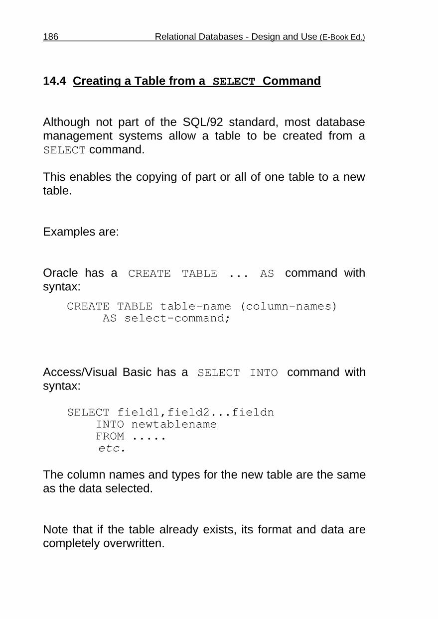
186 Relational Databases - Design and Use (E-Book Ed.)
14.4 Creating a Table from a SELECT Command Although not part of the SQL/92 standard, most database management systems allow a table to be created from a SELECT command. This enables the copying of part or all of one table to a new table. Examples are: Oracle has a CREATE TABLE ... AS command with syntax:
CREATE TABLE table-name (column-names) AS select-command;
Access/Visual Basic has a SELECT INTO command with syntax:
SELECT field1,field2...fieldn INTO newtablename FROM ..... etc.
The column names and types for the new table are the same as the data selected. Note that if the table already exists, its format and data are completely overwritten.

The SQL Data Maintenance Commands 187
14.5 The SQL Command : ALTER TABLE ... ADD Once a table has been created it is possible to add an extra column to the table using the SQL command: ALTER TABLE table-name ADD column-details;
The new columns are added to the existing columns in the table. All rows that already exist in the table will have null values created for the new columns. . .
. . . these may then be altered using the UPDATE command if required. The column details are in the same format as in the CREATE TABLE command. Examples: ALTER TABLE EMP ADD FIRST_NAME VARCHAR(10); ALTER TABLE DEPT ADD RENT MONEY;
Note: Both the CREATE TABLE and the ALTER TABLE commands can be used to create or modify table constraints as well as columns ....
.... constraints are discussed later under database integrity issues.

188 Relational Databases - Design and Use (E-Book Ed.)
14.6 The Oracle Command : ALTER TABLE ... MODIFY
A non standard Oracle command allows changes to the format of existing columns of a table. This is possible even though there are existing rows of data. The syntax is:
ALTER TABLE table-name MODIFY (column-details);
Columns with existing entries cannot change type or be reduced in width - they can only be made wider. ie. Only if all rows have null entries for a column can that column change type or be reduced in width. The ( ) round the column-details are not necessary for single columns. Examples: ALTER TABLE EMP MODIFY ENAME CHAR(12); ALTER TABLE DEPT MODIFY ( RENT NUMBER(5), OWNER CHAR(20) );
Note: In Oracle SQL it is not possible to alter a table to
remove columns.

The SQL Data Maintenance Commands 189
14.7 The SQL Command : ALTER TABLE ... DROP The ALTER TABLE command can also remove a column and any data it contains from a table. The syntax is:
ALTER TABLE table-name DROP column-name;
Example: ALTER TABLE EMP DROP COMM;
Note: Although it is part of the SQL/92 standard the ALTER
TABLE ... DROP command is not available in Oracle SQL.
14.8 The SQL Command : DROP TABLE A whole table is deleted using the SQL command: DROP TABLE The syntax is:
DROP TABLE table-name; Example: DROP TABLE DEPT;

190 Relational Databases - Design and Use (E-Book Ed.)
14.9 The SQL Command : INSERT
Once a table has been created, new rows of data can be added to it with the INSERT command with syntax:
INSERT INTO table-name (columns) VALUES (value-list);
or INSERT INTO table-name (columns)
select-command;
• The (columns) are optional, if omitted all columns are assumed.
• If the columns are named then any unmentioned
columns will be set to NULL. • The first format is used to insert one record at a time
into the table. • The second format is used to copy data from one table
to add it to another. Examples: INSERT INTO dept VALUES (50,'FOREIGN','LONDON'); INSERT INTO emp (empno,ename,hiredate) VALUES (1234,'SANTA','25-DEC-95');
INSERT INTO My_Table (Name,Sal,Department) SELECT ename,sal,dname FROM emp INNER JOIN dept ON emp.deptno = dept.deptno; WHERE job='CLERK';

The SQL Data Maintenance Commands 191
14.10 The SQL Command : DELETE This command is used to delete rows from a table. The general syntax is: DELETE FROM table-name WHERE conditions;
Rows are deleted that match the conditions. Warning: If there is no WHERE clause all rows are deleted, the table will still exist but it will be empty. Examples: DELETE FROM emp; DELETE FROM emp WHERE ename = 'WARD'; DELETE FROM emp WHERE comm IS NOT NULL OR ename LIKE 'A%';

192 Relational Databases - Design and Use (E-Book Ed.)
14.11 The SQL Command : UPDATE This command is used to alter one or more columns in one or more rows of a table. The general syntax is: UPDATE table-name SET column-assignments WHERE conditions;
The column-assignments are a list of assignments separated by commas where each is in the form: column-name = new-value
or column-name = NULL
Warning: If no WHERE clause is specified all rows are updated. Examples: UPDATE emp SET sal = sal*1.1;
UPDATE emp SET job = 'MANAGER', sal = 3000, comm = NULL, deptno = 40 WHERE ename = 'FORD';

The SQL Data Maintenance Commands 193
14.12 Making Data Maintenance Changes
Permanent
Changes made to a data base with INSERT, DELETE or UPDATE are all stored temporarily . . .
. . . they do not permanently alter the data!
To become permanent the following SQL command must be given:
COMMIT;
It is also possible to abandon all changes made in one session since the last COMMIT with the command:
ROLLBACK;
Some commands perform an implicit COMMIT command making all previous changes permanent.
These commands are: CREATE, ALTER or DROP GRANT, REVOKE OR EXIT N.B. The COMMIT and ROLLBACK commands do not exist
in Visual Basic/Access SQL. From a Visual Basic program each command is immediately committed automatically unless the BeginTrans database function is used .... .... in which case the database functions CommitTrans and Rollback provide the functionality of the SQL COMMIT and ROLLBACK commands.

194 Relational Databases - Design and Use (E-Book Ed.)
CHAPTER 15
SQL Subqueries
Contents Page 15.1 Using a SELECT Subquery 195
15.2 SELECT Commands With SELECT Subqueries 196
15.3 Subqueries With ANY, SOME or ALL 197
15.4 Subqueries With IN and NOT IN 198
15.5 The WHERE EXISTS Subquery 199
15.6 Subqueries Needing a Table Alias Name 200
15.7 Different Ways of Making a Subquery 201
15.8 Combining Selections With the UNION Operator 202
15.9 Example Output From a UNION 203
15.10 Distinct Row Output With a UNION 204
15.11 Column Headings With a UNION 204
15.12 Ordering the Output With a UNION 205
15.13 Restrictions On The Use Of a UNION 205
15.14 The INTERSECT and EXCEPT Operators 206
15.15 Oracle and Access Implementations of the UNION, INTERSECT and EXCEPT Operators 207

SQL Subqueries 195
15.1 Using a SELECT Subquery The SELECT command can appear as part of other commands. An example is the INSERT command: INSERT INTO mytable (IDnumber,name) SELECT empno,ename FROM emp WHERE job='CLERK';
The SELECT command can, in fact, appear in any command with a WHERE clause such as DELETE or even SELECT itself: DELETE FROM emp WHERE deptno = (SELECT deptno FROM dept WHERE dname='ACCOUNTING');
This example will delete all records from the EMP table of employees working in the accounts department. In an example of this type it is important that the select command retrieves just one value, or an error will occur. . . . . . It would not make any sense to have more than one value in such a comparison anyway.

196 Relational Databases - Design and Use (E-Book Ed.)
15.2 SELECT Commands With SELECT Subqueries The WHERE clause on the SELECT command can also contain a SELECT subquery. Eg. To find all employees with a salary greater than Scott
use: SELECT ename,sal FROM emp WHERE sal > (SELECT sal FROM emp WHERE ename = 'SCOTT');
It is possible for the subquery to have further subqueries nested to any depth. Eg. To find all employees with a salary greater than the
manager of the accounts department: SELECT ename,sal FROM emp WHERE sal > (SELECT sal FROM emp WHERE job='MANAGER' AND deptno = (SELECT deptno FROM dept WHERE dname='ACCOUNTING'));
Note that the subquery can select from either the same table or a different table to the main SELECT command.

SQL Subqueries 197
15.3 Subqueries With ANY, SOME or ALL It is possible to use subqueries that may give multiple values if ANY, SOME or ALL is used: Example of a subquery used with ANY or SOME: To list all employees earning as much in salary as a
manager:
SELECT ename,sal FROM emp WHERE sal >= ANY (SELECT sal FROM emp WHERE job='MANAGER');
In this example, the WHERE clause will be true if the
subquery search finds any manager's salary less than or equal to the salary of the record currently being examined.
SOME is simply an alternative word for ANY and has the
same meaning. Example of subquery used with ALL: To list the employees with the minimum salary:
SELECT ename,sal FROM emp WHERE sal <= ALL (SELECT sal FROM emp);
This WHERE condition is true only if the salary of the
record currently being examined is less than or equal to every value selected in the subquery.

198 Relational Databases - Design and Use (E-Book Ed.)
15.4 Subqueries With IN and NOT IN An alternative form for a multi-valued subquery is to use the IN or NOT IN conditions: Eg1. To list every department that employs a clerk:
SELECT dname FROM dept WHERE deptno IN (SELECT deptno FROM emp WHERE job='CLERK');
Note: IN (subquery) is another way of writing = ANY(subquery). Eg2. To list every department that has no salesmen:
SELECT dname FROM dept WHERE deptno NOT IN (SELECT deptno FROM emp WHERE job='SALESMAN');
N.B. This would not have been achieved with:
SELECT dname FROM dept WHERE deptno IN (SELECT deptno FROM emp WHERE job!='SALESMAN');
. . . as the sales department would be selected as it has some employees that are not salesmen.
Note: NOT IN (subquery) is another way of writing != ALL(subquery).

SQL Subqueries 199
15.5 The WHERE EXISTS Subquery It is sometimes more convenient or natural to use a WHERE EXISTS or WHERE NOT EXISTS subquery. In the WHERE EXISTS subquery if any matching record is found the result is true, so the column specification in the subquery is irrelevant. Similarly the result is false if any matching record for a WHERE NOT EXISTS subquery is found. Eg. To list every department with employees recorded in the
EMP table:
SELECT dname FROM dept WHERE EXISTS (SELECT * FROM emp WHERE emp.deptno=dept.deptno);
This could also have been achieved using:
SELECT dname FROM dept WHERE deptno IN (SELECT deptno FROM emp);
Similarly to list departments that have no recorded employees:
SELECT dname FROM dept WHERE EXISTS (SELECT * FROM emp WHERE emp.deptno=dept.deptno);
This also has a NOT IN equivalent.

200 Relational Databases - Design and Use (E-Book Ed.)
15.6 Subqueries Needing a Table Alias Name If a subquery selects from the same table as the main query it may be necessary to use a table alias name. Eg. To list all employees who manage other employees: SELECT ename FROM emp AS boss WHERE NOT EXISTS (SELECT * FROM emp WHERE emp.mgr = boss.empno);
In this example if the alias "boss" was not used the subquery would look for all employees who were their own managers!

SQL Subqueries 201
15.7 Different Ways of Making a Subquery A selection using a subquery may be done in different ways.
Eg. The following are equivalent: SELECT ename FROM emp boss WHERE EXISTS (SELECT * FROM emp WHERE emp.mgr=boss.empno);
SELECT ename FROM emp WHERE empno = ANY (SELECT mgr FROM emp);
SELECT ename FROM emp boss WHERE empno IN (SELECT mgr FROM emp);
. . . and frequently the same information can be obtained just as easily using a table join: SELECT DISTINCT boss.ename FROM emp boss INNER JOIN emp slave ON slave.mgr = boss.empno;
On large tables the different methods may give significant differences in speed and efficiency. This is a disadvantage of SQL as it is confusing . . . .
. .users are unlikely to know which is more efficient.
Usually a WHERE EXISTS or WHERE NOT EXISTS subquery is more efficient than other methods.

202 Relational Databases - Design and Use (E-Book Ed.)
15.8 Combining Selections With the UNION
Operator
It is sometimes necessary to select information where each column of output may come from more than one table.
Eg. Suppose a company's database had tables: CUST with columns CNAME for a customer's name and CADDR for the customer's address and
SUPP with columns SNAME for a supplier's name and SADDR for the supplier's address To list all outside organisations that the company deals with would require a selection from each table . . .
. . . but because a supplier may also be a customer for a different product, listing both tables with two SELECT commands would give some names twice. To give the required selection the UNION operator is used to combine SELECT commands: SELECT cname AS Name, caddress AS Address FROM cust UNION SELECT sname, saddress FROM supp;

SQL Subqueries 203
15.9 Example Output From a UNION
The command: SELECT ename,empno FROM emp
UNION SELECT dname,deptno FROM dept;
Gives: ENAME EMPNO ---------- ------ ACCOUNTING 10 ADAMS 7876 ALLEN 7499 BLAKE 7698 CLARK 7782 FORD 7902 JAMES 7900 JONES 7566 MARTIN 7654 MILLER 7934 OPERATIONS 40 RESEARCH 20 SALES 30 SCOTT 7788 SMITH 7369 TURNER 7844 WARD 7521
The command:
SELECT ename,job,deptno FROM emp WHERE job = 'CLERK' UNION SELECT ename,job,deptno FROM emp WHERE deptno = 10;
Gives: ENAME JOB DEPTNO ---------- --------- ------ ADAMS CLERK 20 CLARK MANAGER 10 JAMES CLERK 30 KING PRESIDENT 10 MILLER CLERK 10 SMITH CLERK 20

204 Relational Databases - Design and Use (E-Book Ed.)
15.10 Distinct Row Output With a UNION A UNION implies a SELECT DISTINCT on the resulting output, any rows of output that are duplicated are eliminated. ie. A row will be output only once if it is generated from both the SELECT commands. The output will list duplicates if UNION ALL is used. eg. SELECT ename,job,deptno FROM emp
WHERE job = 'CLERK' UNION ALL SELECT ename,job,deptno FROM emp WHERE deptno = 10;
would cause the row
MILLER CLERK 10
to be output twice. 15.11 Column Headings With a UNION If two columns with different names are combined using the UNION operator, it is the name in the first SELECT that is used in the column header. The header used is the only effect of changing the order in which the SELECT commands are specified...
.... there is no difference in the rows displayed. Any change of header using AS must be specified on the first SELECT command or it will be ignored.

SQL Subqueries 205
15.12 Ordering the Output With a UNION The UNION output is automatically ordered on the first column displayed unless this is changed with an ORDER BY clause. It is not possible to specify individual ORDER BY clauses for each SELECT with a UNION operator but...
. . . a single ORDER BY clause can be used if it is at the end of the whole command. eg. SELECT cname,caddress FROM cust WHERE caddress LIKE '*Loughborough*' UNION SELECT sname, saddress FROM supp ORDER BY cname DESC;
Note that the ORDER BY clause must refer to the column or columns in the first SELECT command. 15.13 Restrictions On The Use Of a UNION 1. The same number of columns must be selected from
each SELECT command. 2. Corresponding columns of each SELECT command
must be of the same type, though it is not necessary for the columns to be the same length.
3. Columns of type MEMO cannot be included. There is no restriction on the number of SELECT commands that may be combined with UNION operators.

206 Relational Databases - Design and Use (E-Book Ed.)
15.14 The INTERSECT and EXCEPT Operators
Like the UNION operator, the INTERSECT and EXCEPT operators operate on selections from more than one table and have the same restrictions and ordering.
Eg. To list all organisations that are both a supplier and a customer use INTERSECT:
SELECT cname "Name", caddress "Address" FROM cust INTERSECT SELECT sname, saddress FROM supp;
Eg2. To list all suppliers that are not also customers use EXCEPT:
SELECT sname "Name", saddress "Address" FROM supp EXCEPT SELECT cname, caddress FROM cust;
With UNION and INTERSECT it does not matter which SELECT is before or after the operator other than the effect on the column header. For the EXCEPT operator the order is significant:
eg. SELECT cname "Name", caddress "Address" FROM cust EXCEPT SELECT sname, saddress FROM supp;
This will select all customers who are not suppliers.

SQL Subqueries 207
15.15 Oracle and Access Implementations of the UNION, INTERSECT and EXCEPT Operators
• Both Oracle and Access/Visual Basic implement the Union operator as described.
• Oracle implements the INTERSECT operator but
Access/Visual Basic does not. • Oracle does not implement the EXCEPT operator but
does implement a MINUS operator that is identical in operation.
• Access/Visual Basic does not implement the EXCEPT
operator and does not have any equivalent.
• In Access/Visual Basic the UNION operator can also be
used to combine the output of two TABLE commands or a TABLE command with a SELECT Command.
Eg. SELECT cname AS [Name], caddress AS [Address] FROM cust WHERE caddress LIKE '*Loughborough*' UNION TABLE supp;

208 Relational Databases - Design and Use (E-Book Ed.)
CHAPTER 16
Views
Contents Page 16.1 What is a View? 209
16.2 How is a View Created Using SQL? 210
16.3 Why Create a View? (1) Security 211
16.4 Why Create a View? (2) Convenient Access to Joined Tables 212
16.5 Why Create a View? (3) Saving Complex Expressions 213
16.6 Why Create a View? (4) Allowing Different Table Formats 214
16.7 Why Create a View? (5) "Tables" of Summary Information 215
16.8 Why Create a View? (6) Logical Data Independence 216
16.9 Data Updates Through a View 217
16.10 Deleting a View 217

Views 209
16.1 What is a View?
A view is a "virtual table".
ie. A user can examine the data it contains as though it was a real table.
In reality it is a "window" onto one or more underlying base tables selecting and arranging the information in its own presentation.
The display of the information in a view is generated at the time it is viewed ....
.... not at the time the view is defined.
Any change to any base table data automatically changes the corresponding information displayed in any associated view.
Many Database Management Systems, such as Oracle, have the capability of creating these views and it is a standard facility of SQL systems. N.B.: A surprising omission of Access/Visual Basic SQL is
that views are NOT implement. However, the Access "Querydef" (which has to be created using Access facilities other than Access SQL) has similar properties to a view.

210 Relational Databases - Design and Use (E-Book Ed.)
16.2 How is a View Created Using SQL? By using the CREATE VIEW command in the form:
CREATE VIEW view-name (column-names) AS select command;
The select command in a view is identical to the usual SQL SELECT command with any clause except the ORDER BY clause. The list of column names in ( ) can give new names to the columns in the view ....
.... they can be omitted, if they are the same names as the base table columns are taken. Example of use of a view:
CREATE VIEW earnings (name,income) AS SELECT ename,sal+NVL(comm,0) FROM emp,dept WHERE emp.deptno = dept.deptno;
(NVL is as Oracle function used here to assign a value of zero to all null fields in the comm column) Example of a view with grouped data:
CREATE VIEW totals (deptno,sal,comm) AS SELECT deptno,SUM(sal),SUM(comm) FROM emp GROUP BY deptno;

Views 211
16.3 Why Create a View?
(1) Security A view can restrict a user's access to a subset of the data in a table .... .... users may be given access to a view where there is no access to the base table(s). Example 1: Restricted access to columns. A library data base may be available to public examination to allow users to see: 1. Which books are available 2. Which books are out on loan but not 3. Who the books are on loan to Example 2: Restricted access to rows: Members of a university department may have access to inspect the university's accounts .... .... but this may be restricted through a view so that only the transactions of that department can be displayed.

212 Relational Databases - Design and Use (E-Book Ed.)
16.4 Why Create a View?
(2) Convenient Access to Joined Tables When there is a need for regularly displaying data from two different, joined tables a view can create a permanent, virtual, composite table. Example There may be a regular need for details of a company's employees along with the details of their department .... .... if this information is stored in two different tables such as the example "emp" and "dept" tables they could be combined into one by using: CREATE VIEW mix_data AS SELECT number,ename,job,dname,place FROM emp,dept WHERE emp.deptno = dept.deptno;
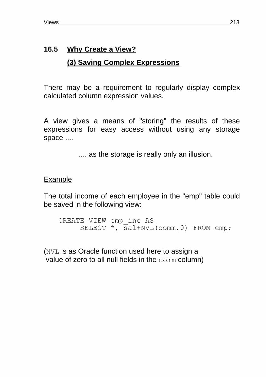
Views 213
16.5 Why Create a View?
(3) Saving Complex Expressions There may be a requirement to regularly display complex calculated column expression values. A view gives a means of "storing" the results of these expressions for easy access without using any storage space .... .... as the storage is really only an illusion. Example The total income of each employee in the "emp" table could be saved in the following view: CREATE VIEW emp_inc AS SELECT *, sal+NVL(comm,0) FROM emp;
(NVL is as Oracle function used here to assign a value of zero to all null fields in the comm column)

214 Relational Databases - Design and Use (E-Book Ed.)
16.6 Why Create a View?
(4) Allowing Different Table Formats
A view can have a different, more convenient, format from that of the base table.
Example 1: Different order of columns
A table may have a column for a person's initials and a column for the surname. Different users may require output in:
1. "Telephone directory" format of: Dawson R.J.
2. The conventional name order of: R.J.Dawson
If suitable views are created these could both be output by SELECT * FROM view-name;
Example 2: Different column formats
In Oracle there is a view called USER_VIEWS gives an output usually longer than one line if all columns are selected.... .... it may be more convenient to create a new view that truncates all columns to, say, half their length so that they fit on one line. This would allow a quick look at the table through the new view in a format that would be easy to read and would serve most purposes.... .... however, where some important details are required that have been cut by the truncation, the full details are still available by accessing the original USER_VIEWS table.

Views 215
16.7 Why Create a View?
(5) "Tables" of Summary Information A view is a convenient way of "storing" grouped data such as totals, averages etc. using group functions - without actually using storage space. Many database management systems have application generation facilities that will build default forms to handle the data in a single table .... .... the use of a view based on group data may enable a default form to be similarly built to handle data from group summary data from a table. Example A company accounting data base may need a view to show numbers of transactions, totals and balances for each department. This virtual table would be produced by a command such as: CREATE VIEW summaries (deptname,transactions,balance) AS SELECT deptname,COUNT(*),SUM(trans) FROM dept_accounts GROUP BY deptname;

216 Relational Databases - Design and Use (E-Book Ed.)
16.8 Why Create a View?
(6) Logical Data Independence A view can be used to make a selection of command procedures and forms independent of the data format.
This is often introduced by necessity if there is a change in base table format as it may: 1. Save retraining users
2. Reduce the need to change any program that accesses the data.
Example The EMP table could at one time have stored only the total income for each employee .... .... later changes in circumstances may have created the necessity to split the income into its salary and commission components.
For this change it is possible to overcome the need to change any existing command files by:
1. Naming the new format EMP table as something other than EMP.
2. Creating a view called EMP on this new table that
recreates the old emp format.

Views 217
16.9 Data Updates Through a View
It is possible to insert or update data though a view in some circumstances. If this is done it is the base tables that are really altered.
Rows can be updated providing:
1. The view is made up from one base table only.
2. None of the columns are derived from an expression.
3. The query to create the view contained no group function, no DISTINCT clause or no GROUP BY clause.
New rows can be inserted if all of the above applies and also if all columns constrained to be not null are included in the view. But note: Rows can never be deleted from a view. 16.10 Deleting a View
Views can be discarded when they are no longer needed using the SQL command DROP VIEW. Eg. DROP VIEW my_view;

218 Relational Databases - Design and Use (E-Book Ed.)
CHAPTER 17
Performance of Relational
Database Management Systems
Contents Page
17.1 Why Are Relational Databases Slow? 219
17.2 Improving Access Time By De-Normalisation 220
17.3 Example 1: De-Normalisation by Adding Fields that are Not Dependent on the Key 221
17.4 Example 2: De-Normalisation by Repeating Fields 222
17.5 Improving Access Time by Using Indexes 223
17.6 How is an Index Used? 224
17.7 Maintaining Indexes 225
17.8 Implications of Index Maintenance 225
17.9 Different Types of Index 226
17.10 Creating an Index in SQL 227
17.11 Improving Access Time by Optimising Queries 228
17.12 The Oracle Query Optimiser 229
17.13 Optimising Join Queries 230
17.14 Join Query 'Search' and 'Driving' Tables 231
17.15 Correct Use of the SQL SELECT Command HAVING and WHERE clauses 232
17.16 Improving Access Using Multiple Disks 233
17.17 Improving Access Time With a Single Disk 233
17.18 Improving Access Time by Maximising Memory Use 234

Performance of Relational Database Management Systems 219
17.1 Why Are Relational Databases Slow? Relational database management systems are relatively easy to use . . .
. . . but they can be very slow in their operation.
Why? 1. The input commands have to be interpreted every time
an instruction is given. 2. Data is stored in no particular order, this means that
searches and sorts are repeated every time a command requires it.
3. Table joins are re-created for every instruction using the
join - even joins made through a view.
This involves a search through one table for a match for every record in the other.
4. Often no advantage can be made of available memory
to store temporary tables, etc. as the system always uses disk storage.
5. The software is general purpose, no advantage is taken
of particular features of an application for optimisation:
eg. A search may only ever produce one record in a particular application - but the search will continue to the end of the table regardless.

220 Relational Databases - Design and Use (E-Book Ed.)
17.2 Improving Access Time By
De-Normalisation
Normalisation of data produces an efficient storage structure .... but it may not produce the most efficient structure for speed of access to the data.
In particular:
Displaying data from two joined tables requires stepping through one table and, for each record to be displayed, searching for a match in the other table....
.... this is very slow if many records are displayed! Depending on the proportion of times the table will be accessed in this way it may be worth de-normalising by merging the tables. Merging tables can be done in two ways:
1. Adding fields that are not dependent on the key if the resulting table has only a limited number of records.
2. Repeating fields if there is a limited number of values in a multi-value dependency.
N.B. Remember! This is not just a trade off of speed verses
storage .... .... it will also make the data more
prone to errors of inconsistency!

Performance of Relational Database Management Systems 221
17.3 Example 1: De-Normalisation by Adding
Fields that are Not Dependent on the Key If some normalised data gave the following tables: Worker Table: WorkerID -> Title, Name, DoB, Grade
Wages Table: Grade -> Wage
If there are only 100 workers, the extra storage required to add the Wage field to the Worker table is negligible. This would give fields:
WorkerID -> Title, Name, DoB, Grade, Wage
This now allows faster access to a workers wage.... but .... • If there were only half a dozen grades the wages for
each grade would be stored many times over. ie. Each time a wage for a grade was altered it would
need to be changed in the table many times.
This is an obvious source of potential error!

222 Relational Databases - Design and Use (E-Book Ed.)
17.4 Example 2: De-Normalisation by Repeating
Fields If some normalised data gave the following tables: Worker Table: WorkerID -> Title, Name, DoB, Grade
Training Table: WorkerID + Qualification If every worker will never have more than three qualifications, the Qualification field could be repeated in the Worker table to give: WorkerID -> Title, Name, DoB, Grade, Qualification1, Qualification2, Qualification3 This will allow faster access to a workers qualifications.... but .... • It will waste space with blank fields if some workers
have less than three qualifications. • It may be more awkward to handle. Eg. Any search for a particular qualification would
require searching all three qualification fields.
Another obvious source of potential error!

Performance of Relational Database Management Systems 223
17.5 Improving Access Time by Using Indexes What is an Index? An index is formed on one or more columns in a table.
It is a table of row identifiers in the order of the given columns (the exact format is DBMS dependent). Why use an index? Once an index is made it is much faster to:
1. Sort the table on the given column(s).
2. Search the table for a particular column value - particularly significant for joins.
3. Select records using conditional clauses such as field_value < constant_value.
ie. The use of an index can greatly speed up a display command, especially for tables joined on the given column(s).
But is there any overhead? 1. Extra storage is required for the index equivalent to an
extra column in the table.
2. Extra disk access means an index will only improve the speed of a display if less than 25% (approx) of the records are selected for display.

224 Relational Databases - Design and Use (E-Book Ed.)
17.6 How is an Index Used?
On many database management systems the user need take no special action to use an index .... The D.B.M.S. will use an index automatically where
appropriate.
However an index may not be used if:
1. The index column is used in an expression
2. The column is tested to be NULL or NOT NULL
Sometimes it is possible to re-format a conditional clause so that an index may be used where its use was previously prevented. . .
. . . or vice-versa if it is likely that more than 25% of the records will be selected.
For example, if the column 'number' was indexed the index would normally be used in the expression:
WHERE number > 200/1.15
but it may not be in: WHERE number*1.15 > 200 and the index would normally be used in:
WHERE number > 0
but it may not be in: WHERE number IS NOT NULL
It is up to the designer of database applications to know the behaviour of the system used.

Performance of Relational Database Management Systems 225
17.7 Maintaining Indexes Whenever any insert, update or delete is done, it is necessary to update all the indexes for that table ....
.... most D.B.M.S.s do this automatically. ie. Once an index is created the user can usually forget
about it ....
.... the D.B.M.S. will do all that is necessary to use and maintain it.
17.8 Implications of Index Maintenance Keeping an index up to date takes some processing time, every time any alteration is made to the table. ie. In order to decide whether to create an index the
balance must be considered: Frequency of Frequency of sorting or adding to or selecting on modifying the column(s) the table

226 Relational Databases - Design and Use (E-Book Ed.)
17.9 Different Types of Index Unique Indexes SQL allows an index to be specified as "unique". A unique index is one where every entry in the column or combination of columns is unique ....
.... a unique index can be used more effectively for table searching, speeding up a search operation.
A unique index also helps preserve the integrity of a column by preventing any error of the same value appearing twice. Additional Non Standard Index Types 1. Indexes in Oracle
These can be "compressed", which takes less disk space, or "non compressed", which takes more space but allows faster searches.
This can help to further improve performance.
2. Indexes in Visual Basic/Access
These can prevent a column having null entries, can specify a column as a "primary" key or as a "foreign" key.
This can help to secure the database integrity.

Performance of Relational Database Management Systems 227
17.10 Creating an Index in SQL An index is created with the SQL command:
CREATE [UNIQUE] INDEX index-name ON table-name ( column(s) );
If more than one column is specified the rows are sorted in the order of the first mentioned column, then where values are the same, in the order of the second column, etc. Examples: CREATE INDEX nameidx ON emp(ename,deptno); CREATE UNIQUE INDEX empindex ON emp(empno);
How Many Indexes Can a Table Have?
A table can have any number of indexes. . .
. . . but as each index takes storage space there may be limitations. How is an Index Deleted?
The standard SQL command to delete an index is:
DROP INDEX index-name;
In Visual Basic/Access SQL, however, it is necessary to specify the table name in the DROP command:
DROP INDEX index-name ON table-name;

228 Relational Databases - Design and Use (E-Book Ed.)
17.11 Improving Access Time by Optimising
Queries The structure and order of a query with multiple conditions as the selection criteria can effect the speed in which it can operate. • A multiple selection criterion of the form:
WHERE condition1 AND condition2
will be faster if condition1 eliminates more records than condition2.
• A multiple selection criterion of the form:
WHERE condition1 OR condition2
will be faster if condition1 selects more records than condition2.
But .... if an index column is being tested: • An indexed field should be tested before any other field.
• A unique indexed field should be tested before any non unique indexed field.
But note: The D.B.M.S. may do this optimisation of indexed columns for you automatically!

Performance of Relational Database Management Systems 229
17.12 The Oracle Query Optimiser Oracle will automatically try and optimise the order in which it tackles multiple queries as follows: 1. Indexed column queries come before non-indexed
column queries. 2. Unique index queries come before non-unique index
queries. 3. Non-compressed index queries come before
compressed index queries. 4. ROWID queries come before column and expression
queries. 5. Queries with = come before queries with a range of
values. 6. Bounded range queries come before unbounded range
queries. Any ordering of queries by the user is only effective if the queries are "equal" by the above rules.

230 Relational Databases - Design and Use (E-Book Ed.)
17.13 Optimising Join Queries If there is a join of two or more tables then the join condition should be placed last. Eg. Consider the workers example which had the following tables:
Wage Table: Grade -> Wage
Worker Table: WorkerID -> Title, Name, DoB, Grade To find a worker's wage given his name the SQL command could be:
SELECT Name,Wage FROM Workers,Wages WHERE Workers.Grade = Wages.Grade AND Name = 'Bloggs J.';
This would join the entire Workers table with the Wages table and then, from the result, select the joined record for the name 'Bloggs J.'. Alternatively, it would be much faster to use:
SELECT Name,Wage FROM Workers,Wages WHERE Name = 'Bloggs J.' AND Workers.Grade = Wages.Grade;
This would select the single record from the Wages table with name 'Bloggs J.' and then find the corresponding record in the Wages table.

Performance of Relational Database Management Systems 231
17.14 Join Query 'Search' and 'Driving' Tables
When tables are joined in a query, either table can be the search table or driving table.
ie. The D.B.M.S. steps through every record in the driving table and looks for a match in the joined, search table.
The choice of which table is the driving table and which is the search table can greatly affect the speed of the query:
• If one of the tables is joined on an indexed column it is more efficient to make this the search table.
• If both tables are joined on indexed columns but only one index is unique, then this should be the column in the search table.
• If both columns are of equal type it is more efficient to make the table with the smaller number of relevant rows the driving table....
ie. Reduce the number of searches to be made.
Often the order in which the tables are specified determines which is the driving table and which is the search table. Example: 'Oracle' takes the first mentioned in the query as
the search table. But note: The D.B.M.S. may automatically optimise table
joins involving an index.
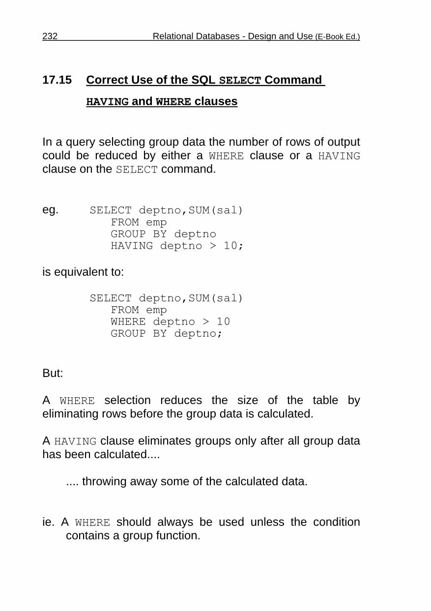
232 Relational Databases - Design and Use (E-Book Ed.)
17.15 Correct Use of the SQL SELECT Command
HAVING and WHERE clauses In a query selecting group data the number of rows of output could be reduced by either a WHERE clause or a HAVING clause on the SELECT command. eg. SELECT deptno,SUM(sal)
FROM emp GROUP BY deptno HAVING deptno > 10; is equivalent to: SELECT deptno,SUM(sal) FROM emp WHERE deptno > 10 GROUP BY deptno; But: A WHERE selection reduces the size of the table by eliminating rows before the group data is calculated. A HAVING clause eliminates groups only after all group data has been calculated.... .... throwing away some of the calculated data. ie. A WHERE should always be used unless the condition
contains a group function.

Performance of Relational Database Management Systems 233
17.16 Improving Access Using Multiple Disks
If the database can be spread over several disks then access speed can be affected by the placing of tables and indexes on different disks. Eg. Searching on an indexed column involves two disk accesses to obtain each record, one for the index and one for the table ....
.... faster access may be achieved by putting the index and table on different disks to minimise the movement of the disk heads. For the same reason it may be effective to put tables that are frequently joined onto different disks. 17.17 Improving Access Time With a Single Disk
Some database management systems allow some control over tables storage on an individual disk. Eg. Oracle achieves this by using of table "clusters" which store related data items that are used together in the same disk segment. Clustering will usually improve access times, especially for tables joined on the cluster column.... and ... it may also reduce disk storage requirements but ... you must know what you are doing or it can have
the opposite effect!

234 Relational Databases - Design and Use (E-Book Ed.)
17.18 Improving Access Time by Maximising
Memory Use Database management systems tend to be slow simply because disc space is the normal means for storing data. Even if the hardware used has vast amounts of spare memory, this is usually ignored. Some database management systems provide a means for using available memory, but the method is different for each system. Eg. Oracle provides the SET ARRAYSIZE command to
specifies how many records can be held in the host computer's memory at one time.
The default is 20 but up to 5000 can be specified. Using the system's spare memory may be a simple way of improving performance if the D.B.M.S. provides this level of control.

Designing the Database for Integrity 235
CHAPTER 18
Designing the Database
for Integrity
Contents Page 18.1 What is Database Integrity? 236
18.2 Examples of Human Error Damaging System Integrity 237
18.3 Reducing Error With Default Values 238
18.4 Default Field Value Example 239
18.5 Reducing Error by Constraining the Data 240
18.6 CHECK Constraints 241
18.7 Notes on CHECK Constraints 242
18.8 Constraint Names 243
18.9 Assertions 244
18.10 Reducing Error with Mandatory Fields 245
18.11 Access/Visual Basic Mandatory Fields 246
18.12 Reducing Error by Enforcing Unique Values 247
18.13 Adding and Deleting UNIQUE Constraints 248
18.14 Temporary Use of the UNIQUE Constraint 249

236 Relational Databases - Design and Use (E-Book Ed.)
18.1 What is Database Integrity? Database integrity is all about keeping the data meaningful and free from error. Errors can come from two sources:
1. program error
2. human error Program error can be eliminated by careful design and thorough testing ....
.... human error is harder to control! It is possible for the database system to be designed to reduce the chances of human error: • There may be checks built into the database
management system that will automatically be used to reduce input error.
• There are further checks that can be added by the
programmer when tailoring a database system to a particular user's needs.
• The data structure design itself can reduce error. This last method of reducing error can be achieved through normalisation.

Designing the Database for Integrity 237
18.2 Examples of Human Error Damaging
System Integrity Human error can damage the system integrity when:
1. The wrong input is entered.
Eg. Entering a new employee with an ID number that is already used for another person
2. A modification is made that is incomplete
Eg. Deleting a employee's record without altering other tables that refer to the employees ID number.
3. An inexperienced user changes the data without
realising.
Eg. A user may try to get out of the system by typing "exit" and accidentally insert the word into a database field.
4. More than one user at a time tries to alter the same
data.
Eg. Each may read the data at the same time to find the next free ID number and then each assigns the same number to a new entity.
All of these human errors can be reduced by careful system design.

238 Relational Databases - Design and Use (E-Book Ed.)
18.3 Reducing Error With Default Values One way of reducing human error is to minimise the need for manual input of data.
Eg. By entering a pre-defined default value in a table field if no value is otherwise specified in a new record.
In SQL/92 a default value can be specified when the column is defined in the CREATE TABLE or ALTER TABLE ... ADD commands. If no default is specified then a null value default is assumed. The format for specifying a column default is: CREATE TABLE tablename ( ..........., columnname datatype DEFAULT value, ...........); ALTER TABLE tablename ADD columnname datatype DEFAULT value;
where the value is either a constant or NULL. In Oracle SQL it is possible to modify the default value using the ALTER TABLE ... MODIFY command: ALTER TABLE tablename MODIFY columnname DEFAULT value;

Designing the Database for Integrity 239
18.4 Default Field Value Example The effect of the commands: CREATE TABLE employee ( empno INTEGER, ename CHAR(15), job CHAR(10) DEFAULT 'CLERK', sal INTEGER DEFAULT 1000, dept SMALLINT ); ALTER TABLE employee ADD comm INTEGER DEFAULT 0; INSERT INTO employee(empno,ename) VALUES (1234,'SMITH'); INSERT INTO employee(empno,ename,sal) VALUES (1235,'JONES',1200);
would be to create a new table with the following two rows of data: empno ename job sal dept comm
1234 SMITH CLERK 1000 <NULL> 0 1234 JONES CLERK 1200 <NULL> 0
N.B. The DEFAULT clause is NOT available in Access/Visual
Basic SQL. However, an identical facility is available by setting the DefaultValue property for the table fields.

240 Relational Databases - Design and Use (E-Book Ed.)
18.5 Reducing Error by Constraining the Data The SQL/92 standard allows constraints to applied to table data. The constraints are used to: 1. Check specified conditions relating to the table fields are
always satisfied. 2. Check specified columns always contain unique values. 3. Specify table key fields and associated foreign key fields
in other tables. The constraints come in three forms. 1. Column constraints which refer to an individual column. 2. Base table constraints which refer to more than one field
in a single table. 3. Assertion constraints which refer to fields from different
tables.
Note: (1) is just a special case of (2), which in turn is a special case of (3).
But... Neither Oracle or Access/Visual Basic implements
constraints of type (3).

Designing the Database for Integrity 241
18.6 CHECK Constraints A CHECK constraint is specified for a column in the form:
CREATE TABLE tablename ( ..............., columnname datatype CHECK condition, ...............);
Eg. CREATE TABLE person ( idnum SMALLINT CHECK idnum > 0, title CHAR(4) CHECK title IN ('MR','MRS','MISS','MS'), name CHAR(20) );
A CHECK constraint for the base table is specified in the form:
CREATE TABLE tablename ( columnname datatype, ...etc........, CHECK condition, ...etc........, );
Eg. CREATE TABLE person ( idnum SMALLINT, title CHAR(4), name CHAR(20), sal INTEGER, comm INTEGER, CHECK title IN ('MR','MRS','MISS','MS'), CHECK sal+comm < 3000 );

242 Relational Databases - Design and Use (E-Book Ed.)
18.7 Notes on CHECK Constraints 1. The constraint will prevent any row being inserted into
the table or being modified such that the constraint condition is violated....
.... the error message generated, if
any, will depend on the system. 2. In the SQL/92 standard the condition can be any type of
condition that can appear in a WHERE clause. 3. In some database management systems, such as
Oracle, conditions can not involve fields from other rows in the same table or any fields from other tables....
.... this rules out the use of any select subquery in the condition.
4. Access/Visual Basic SQL does not implement CHECK
constraints, but the same effect can be achieved by setting the validation properties of a table record or field.
5. Unlike other types of constraint (described later) there is
no significant difference between a column CHECK constraint and a base table CHECK constraint.

Designing the Database for Integrity 243
18.8 Constraint Names Each constraint can be given a name if the CHECK keyword is preceded by: CONSTRAINT constraintname.
Eg. CREATE TABLE person ( idnum SMALLINT, title CHAR(4) CONSTRAINT tcon CHECK title IN ('MR','MRS','MISS','MS'), name CHAR(20), sal INTEGER, comm INTEGER, CONSTRAINT scon CHECK sal+comm < 3000 );
Constraints can then be dropped and base table constraints added using the ALTER TABLE command with a DROP CONSTRAINT or ADD CONSTRAINT clause.
Eg. ALTER TABLE person DROP CONSTRAINT scon;
ALTER TABLE person ADD CONSTRAINT scon2 CHECK sal+comm < 4000;
In Oracle column constraints can be modified as in:
ALTER TABLE person MODIFY CONSTRAINT scon CHECK sal+comm < 4000; In Oracle a constraint cannot be dropped, but it can be disabled if the CHECK condition is followed by the key word DISABLE.

244 Relational Databases - Design and Use (E-Book Ed.)
18.9 Assertions SQL/92 also offers the ability to create CHECK constraints that are not attached to any particular table. This is done with the CREATE ASSERTION command which has the format: CREATE ASSERTION assertionname CHECK condition;
As it is not in the context of any table the condition necessarily involves SELECT subqueries. Eg. CREATE ASSERTION balance
CHECK (SELECT startbalance FROM accountstable WHERE accnum=12345678) + (SELECT SUM(transaction) FROM logtable WHERE accnum=12345678) = (SELECT endbalance FROM accountstable WHERE accnum=12345678);
The assertion can be dropped using the command: DROP ASSERTION balance;
But .... few database management systems implement this SQL/92 facility, and neither Oracle nor Access/ Visual Basic recognises the assertion commands.

Designing the Database for Integrity 245
18.10 Reducing Error with Mandatory Fields In many Database Management Systems it is possible to prevent a null value being entered into a particular field ...
... this is particularly useful for key fields. In SQL this is done by adding the words NOT NULL after the field type in the CREATE TABLE command: Eg. CREATE TABLE Person(
fname CHAR(20) NOT NULL, sname CHAR(20) NOT NULL, salary INTEGER, comm INTEGER); These constraints can also be given names as in: CREATE TABLE Person( fname CHAR(20) CONSTRAINT fnotnull NOT NULL, sname CHAR(20) CONSTRAINT snotnull NOT NULL, sal INTEGER, comm INTEGER); The NOT NULL constraint is in fact a short form of writing: CHECK columnname IS NOT NULL
so it can be dropped or added as a base table constraint like any other CHECK constraint.

246 Relational Databases - Design and Use (E-Book Ed.)
18.11 Access/Visual Basic Mandatory Fields
Access/Visual Basic SQL does not implement the CHECK constraint and, therefore, does not implement the NOT NULL constraint.... But .... it is still possible to define mandatory fields using an additional index facility.
In Visual Basic/Access the table must first be created with the standard CREATE TABLE command. An index can then be formed on the column or columns concerned with the extra syntax:
CREATE INDEX PersIndx ON Person(fname,sname) WITH DISALLOW NULL;
This would prevent either the fname or the sname fields being made null when a row is inserted or modified.
The index can be either an ordinary index or a unique index as required.
It can also be useful to create and then delete an index with the "DISALLOW NULL" option as a means of checking for null fields in the table. It is also possible to achieve the same effect as the "NOT NULL" clause in Access or Visual Basic by setting the 'Required' property on a table field.

Designing the Database for Integrity 247
18.12 Reducing Error by Enforcing Unique
Values
SQL/92 offers a form of constraint that enforces all column entries to be unique within a table.
A single column can be made to be unique in each row by adding the keyword UNIQUE in the column definition: Eg. CREATE TABLE person (
idnum INTEGER NOT NULL UNIQUE, name CHAR(20), sal INTEGER ); A combination of columns can be made to be unique in each row by adding the UNIQUE base table constraint. CREATE TABLE person ( fname CHAR(12) NOT NULL, sname CHAR(12) NOT NULL, sal INTEGER, UNIQUE(fname,sname)
); In SQL/92 specifying UNIQUE on a column means at most one row can have a null value for this column. Alternatively some database systems assume:
1. The UNIQUE constraint also implies NOT NULL.
or 2. The UNIQUE constraint is not permitted unless NOT NULL is also specified.

248 Relational Databases - Design and Use (E-Book Ed.)
18.13 Adding and Deleting UNIQUE Constraints Like all constraints the UNIQUE constraint can be named, and in Access/Visual Basic SQL this must be done as in:
CREATE TABLE person ( fname CHAR(12) NOT NULL, sname CHAR(12) NOT NULL, sal INTEGER, CONSTRAINT key UNIQUE(fname,sname)
); This then allows the constraints to be dropped or added with the ALTER TABLE command.
Eg. ALTER TABLE person ADD CONSTRAINT key UNIQUE(fname,sname);
ALTER TABLE person DROP CONSTRAINT key;
Most database systems implement the UNIQUE constraint by creating a UNIQUE INDEX with the same name as given to the constraint. The above commands are therefore identical to:
CREATE UNIQUE INDEX key ON person(fname,sname);
DROP INDEX key;
Both Oracle and Access/Visual Basic implement the UNIQUE constraint by creating a UNIQUE index. The error message, if any, for any attempted UNIQUE constraint violation will depend on the system.

Designing the Database for Integrity 249
18.14 Temporary Use of the UNIQUE Constraint As the UNIQUE constraint is usually implemented with a unique index it has the same overhead as a unique index .... ie. Extra disk space is needed and there is some delay on
maintenance operations. It may be useful, therefore, to create the constraint or index temporarily as a test for uniqueness.... ....if the constraint or the index cannot be created then the column or columns are not unique and an error is generated.... ....the constraint or index can then be dropped once the test has been made. As a matter of good practice.... .... if the database system does not provide a UNIQUE constraint or index facility, a search should always be made to ensure any new value for a unique field does not already exist.

250 Relational Databases - Design and Use (E-Book Ed.)
CHAPTER 19
Referential Integrity
Contents Page 19.1 Reducing Errors by Knowing the Foreign Keys 251
19.2 Action To Taken When a Record Is Deleted 232
19.3 Master-Detail Tables 253
19.4 Preventing a Deletion 254
19.5 Action To Taken When a Key Field Is Modified 255
19.6 Enforcing Referential Integrity 256
19.7 Further Referential Constraint Syntax 257
19.8 Notes on Referential Constraints 258
19.9 The ON DELETE Clause 259
19.10 The ON UPDATE Clause 260
19.11 Oracle and Access/Visual Basic 260 Limitations

Referential Integrity 251
19.1 Reducing Errors by Knowing the Foreign
Keys Whether a table structure is derived with entity relationship analysis or by normalisation, a knowledge of the key fields can help secure data integrity. As well as its own key a table may have a field or fields that correspond to the key to another table....
.... this is called a foreign key. When a record from a table is deleted or a key field is modified, it is essential to know which other tables contain the key field(s) as a foreign key....
.... ALL tables containing the corresponding foreign key will also need to be modified!
If these foreign key fields are left unchanged the database will lose its integrity.
If a record is to be deleted action must be taken to either:
1. Set the corresponding foreign key fields to null or default values.
2. Delete the records containing the foreign key values.
3. Prompt the user to enter another foreign key value.

252 Relational Databases - Design and Use (E-Book Ed.)
19.2 Action To Taken When a Record Is Deleted The action to be taken when a key field is deleted will depend on the tables and situation concerned. Consider a company employee details table. The key field, the person ID, may be a foreign key in:
1. a table of previous jobs in other companies
2. a table of who drives each company car Suppose a person record is to be deleted (he or she has left the company). The previous job table entries for the corresponding foreign key value will only be relevant to that person. ie. The corresponding previous job records can also be
deleted. For the company car table, the car will continue to exist, so the car record cannot be deleted! If a car can exist without being allocated to a person (it becomes a pool car) the record in the car table can be set to null....
.... otherwise the car must be reallocated to another person.

Referential Integrity 253
19.3 Master-Detail Tables
For some entities, instances of that entity only exist because of an instance of another, different entity. These are detail entities, each owing their existence to a master entity.
There are two types of master-detail relationships:
1. A detail entity table where each instance is associated with only one of the master entity.
Eg. A previous job table where each record corresponds to just one person entity record.
Instances of previous jobs are usually created when the associated person instance is created.
Such detail table records are deleted when the corresponding master record is deleted.
2. A detail entity table where each instance may be associated with several instances of the master entity.
Eg. A job title table where each title may be associated with several person entity records.
A job title is created when a person instance is created only if the job title does not already exist.
Such detail table records would be deleted when no corresponding master records remain.

254 Relational Databases - Design and Use (E-Book Ed.)
19.4 Preventing a Deletion Suppose the company's employee records also contain a table of who had worked on which projects in the last month. This project table is of historical interest so the records would need to be kept .... .... but the record would make no sense without the details in the original person record .... .... so the person record cannot be deleted! ie. The foreign keys in other tables may mean a record
cannot be deleted!

Referential Integrity 255
19.5 Action To Taken When a Key Field Is
Modified
If a records key field is modified rather than deleted then the actions taken on corresponding foreign keys can be similar to the actions for deletion. There is also the additional option of modifying the foreign keys in step with the original record. Eg. Suppose the company employee record contained the
key field of a company car record (rather than vice-versa as in the last example) ....
.... and suppose also the car registration
number was the company car key field. If the car is replaced, the registration number would
change - and in this case the person record would need to have the same update.
Note: Modifying a tables key fields is questionable ....
.... is it really correct to do so?
In the above example it may be better to delete the old car's record and insert the new car as this more accurately reflects the real world action.
To preserve integrity it may be better to prevent any modification to any key field in any table!

256 Relational Databases - Design and Use (E-Book Ed.)
19.6 Enforcing Referential Integrity SQL/92 provides constraint facilities to enforce referential integrity. ie. It ensures that every foreign key relates to a valid entry
in the table it references. In SQL/92 it is possible to specify the primary key for a table and foreign keys referring to fields in other tables. This is done when creating the table: Eg. CREATE TABLE person (
idnum INTEGER PRIMARY KEY, name VARCHAR(20), deptno INTEGER REFERENCES dept(deptno) );
It is not possible to delete a record in a table if there is any instance of a reference to it by a foreign key field in another table. Eg. If any record in the person table above has a deptno
with value 10, then the corresponding dept table record with deptno value 10 cannot be deleted.
But note - any error message generated will depend on the database system .... in Access/Visual Basic SQL NO error message is given.

Referential Integrity 257
19.7 Further Referential Constraint Syntax The specification of primary and foreign keys can also be a base table constraint.
Eg. CREATE TABLE person (
fname CHAR(20), sname CHAR(20), deptno INTEGER, PRIMARY KEY (sname,fname), FOREIGN KEY (deptno) REFERENCES dept(deptno) );
This is the only way of defining multiple field keys. Like other constraints, referential constraints can be named and handled in the ALTER TABLE command.
Eg. CREATE TABLE person ( idnum INTEGER CONSTRAINT pkey PRIMARY KEY
name CHAR(20), deptno INTEGER, CONSTRAINT fkey FOREIGN KEY (deptno) REFERENCES dept(deptno) );
ALTER TABLE person DROP CONSTRAINT fkey; ALTER TABLE person ADD CONSTRAINT newkey FOREIGN KEY(name) REFERENCES employee(ename);
Note in Access/Visual Basic SQL all constraints must be named.

258 Relational Databases - Design and Use (E-Book Ed.)
19.8 Notes on Referential Constraints
1. There can only be one primary key for a table but there
can as many foreign keys as required.
There can be any number of foreign keys in different tables referencing the same column or columns in one table.
2. A PRIMARY KEY constraint automatically makes the designated fields both UNIQUE and NOT NULL.
3. Most database systems create a unique index on the fields of the primary key constraint.
The primary key can then be dropped with the DROP INDEX command.
4. Before a foreign key can be created it is necessary to either:
• Create a primary key constraint on the referenced column(s) in the referenced table.
• Create a unique constraint or index on the referenced column(s) in the referenced table.
5. If the column(s) in the referenced table are not specified then the primary key of the referenced table is assumed.
Eg. CONSTRAINT fkey
FOREIGN KEY deptno REFERENCES dept

Referential Integrity 259
19.9 The ON DELETE Clause
The SQL/92 default is to prevent the deletion of any row in a table if it has a field with a value referenced by a foreign key in another table. Alternative actions can be specified, however, by adding one of the following to the foreign key definition: ON DELETE CASCADE ON DELETE SET NULL ON DELETE SET DEFAULT
Eg. CREATE TABLE person (
idnum INTEGER PRIMARY KEY, name CHAR(20), deptno INTEGER REFERENCES dept(deptno) ON DELETE CASCADE );
CASCADE means that when the delete is attempted on the row in the dept table referenced by the deptno field in the person table....
1. the delete in the dept table is permitted.
2. all rows in the person table that reference the deleted dept table row will also be deleted.
SET NULL also permits the delete in the dept table but then sets the corresponding foreign key fields in the person table to NULL. SET DEFAULT is similar to SET NULL except the foreign key fields are set to their default values.

260 Relational Databases - Design and Use (E-Book Ed.)
19.10 The ON UPDATE Clause
The ON UPDATE clause is similar to the ON DELETE clause except that it refers to the action taken when a referenced field is modified rather than deleted. The SQL/92 default action is to prevent the modification, but this can be altered if any of the following are specified in the definition of the foreign key:
ON UPDATE CASCADE ON UPDATE SET NULL ON UPDATE SET DEFAULT
CASCADE permits the update and causes the foreign keys to be updated in step with the referenced field. SET NULL permits the update but then sets the corresponding foreign key fields to NULL. SET DEFAULT is similar to SET NULL except the foreign key fields are set to their default value. 19.11 Oracle and Access/Visual Basic Limitations
• Oracle only implements the ON DELETE CASCADE option. The other ON DELETE options and the ON UPDATE options are not recognised.
• Access/Visual Basic SQL does not implement the ON
DELETE or ON UPDATE options, but it is possible to achieve cascade deletes and updates by setting relation attributes.

Designing the User Interface for Integrity 261
CHAPTER 20
Designing the User Interface
for Integrity
Contents Page 20.1 Reducing Human Error With Automatic Generation of Identifier Values 262
20.2 Re-using Identity Numbers 263
20.3 Automatic Generation of Master Identifiers in Detail Tables 264
20.4 Eliminating the Need to Remember Identifiers 265
20.5 Reducing Input Error By Informing the User of Input Types 266
20.6 Reducing Input Error By Displaying Input Values 267
20.7 Reducing Input Error By Checking Input Values 268
20.8 Reducing Input Error By Restricting Input To a Limited List of Values 269
20.9 Password Protection 270
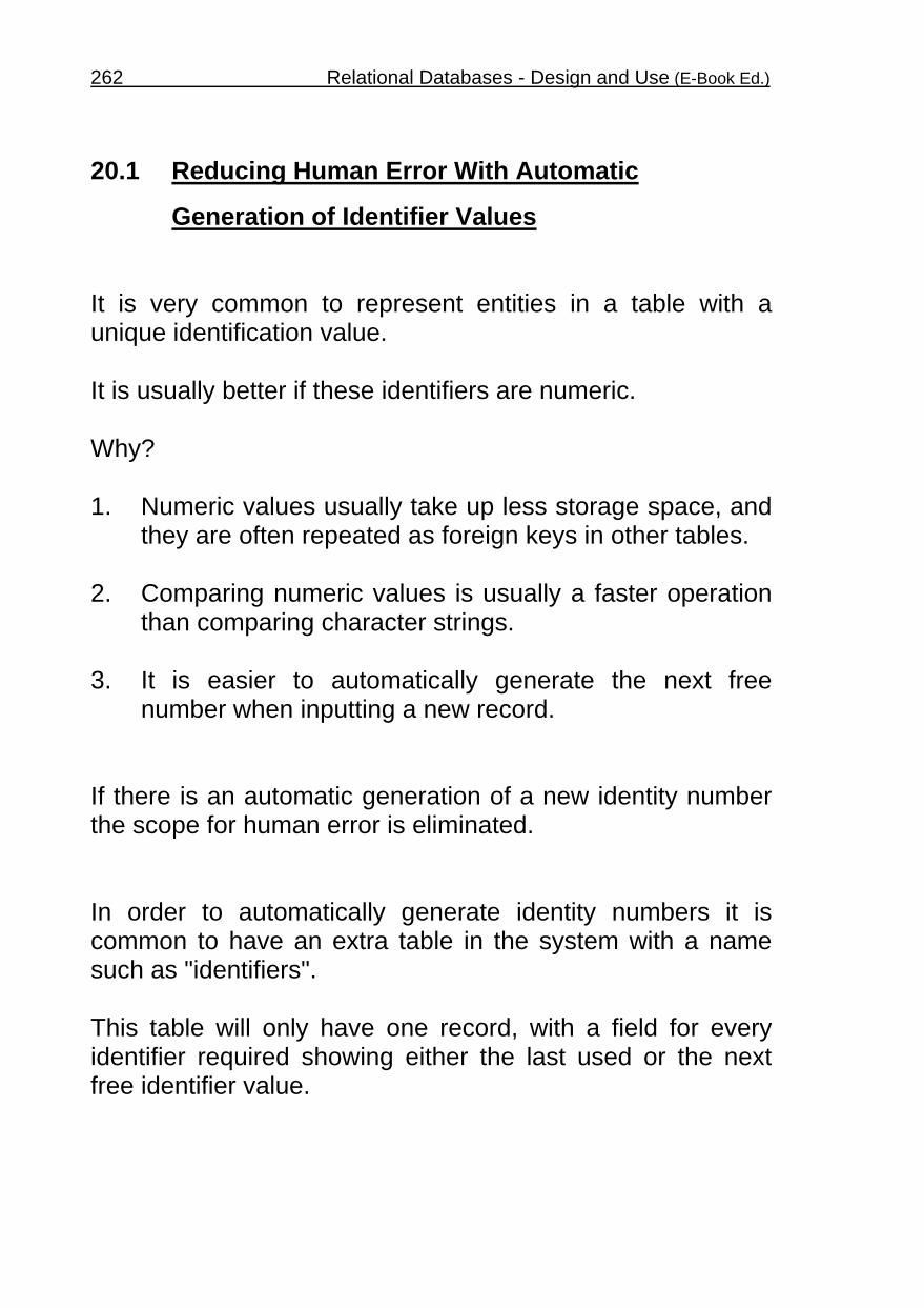
262 Relational Databases - Design and Use (E-Book Ed.)
20.1 Reducing Human Error With Automatic
Generation of Identifier Values It is very common to represent entities in a table with a unique identification value. It is usually better if these identifiers are numeric. Why? 1. Numeric values usually take up less storage space, and
they are often repeated as foreign keys in other tables. 2. Comparing numeric values is usually a faster operation
than comparing character strings. 3. It is easier to automatically generate the next free
number when inputting a new record. If there is an automatic generation of a new identity number the scope for human error is eliminated. In order to automatically generate identity numbers it is common to have an extra table in the system with a name such as "identifiers". This table will only have one record, with a field for every identifier required showing either the last used or the next free identifier value.

Designing the User Interface for Integrity 263
20.2 Re-using Identity Numbers Question.: When a record is deleted how can an
automatic system re-use the spare identifier? Answer: It must not do so! Such re-use is an open invitation for mistakes to happen....
.. identity numbers should remain unique for all time! Eg. Suppose bank were in the habit of re-using an account
number after someone closed their account .... .... then one day a cheque, written by an original account
number owner, is lost in the post but turns up much later ....
.... the new account owner will not be too pleased! An identity number field may be defined to have only a limited number of digits - so it is conceivable the system will run out of numbers .... .... but, it is far better to redefine the field to hold more digits than risk the potential confusion of re-using identity numbers.

264 Relational Databases - Design and Use (E-Book Ed.)
20.3 Automatic Generation of Master
Identifiers in Detail Tables
The generation of input "form" screens of many database management systems is based round forms that correspond to underlying tables. Repeated attributes of an entity are normally put into a separate "detail" table which contains the key to the "master" table as a foreign key. Eg. An employee master table may have an associated
detail table of past positions held. Input of a new "master" entity will therefore require input via several screen "forms", one for the master and one for each detail table. To reduce human error on input the system should:
1. Automatically present the user with the each detail screen in turn when the master screen input is finished.
2. Automatically fill in the foreign master key fields in each detail table.
3. Ideally, allow the user to swap backwards and forwards between the master and detail screens.
This will allow the detail screens to be treated as an extension of the master screen.

Designing the User Interface for Integrity 265
20.4 Eliminating the Need to Remember
Identifiers
Users of many database systems can be seen using a pen and paper to write down values read from the screen that they will need to enter later.
Eg. A company's employee records contain the addresses of each person. One employee gives his name and reports a change of address. The database system operator may have to:
1. Select a search option. 2. Search through the records to find the employee's ID number. 3. Write down the ID number. 4. Select a modify option. 5. Enter the ID number of the record to modify. 6. Change the address.
This use of pen and paper is error prone and a sure sign of a poorly designed database system.
The system should have been designed to either:
1. Allow the user to enter modify mode directly from the search mode to modify the found record.
2. Allow the employees name to be used as an alternative to entering the ID number to identify the record to modify.
However it is done, all need for operators to remember data should be eliminated.

266 Relational Databases - Design and Use (E-Book Ed.)
20.5 Reducing Input Error By Informing the
User of Input Types
This can be achieved in a number of ways: 1. Providing Context Sensitive Help
Help for the current input field can be made available on part of the screen, or in a separate small window,
either: automatically, when the field is entered
or: on request, with a special key combination or button. This is particularly useful to inform the user of the input type, such as the format for date input.
2. Identifying Mandatory Input Fields
Most input forms have some fields that must be filled in for the form to make sense and other fields that may be left blank.
It is possible to prevent the user putting a blank field into the database by specifying the field as NOT NULL
But ... it is less confusing for the user if the form:
1. Clearly identifies mandatory fields eg. by the use of colour.
2. Prevents the user moving to another field until an entry has been made.

Designing the User Interface for Integrity 267
20.6 Reducing Input Error By Displaying
Input Values
1. Defaults Default input values save time and help to reduce input errors, particularly on large forms or forms that are going to be filled in many times over.
SQL/92 provides a default facility to ensure a suitable default value is always entered into the database if the field is unspecified.
But... it is also useful to display the default in the input field on the screen so that:
1. The user knows the value of the default
2. The user can choose whether to overwrite the default or not.
2. Input Verification Fields It is common for a user to enter an identification number to select a record for modification or deletion ....
.... but numeric values are easily miss typed.
In all such cases the user should be given an immediate display of other associated information, such as a name, to allow the user to verify the input.

268 Relational Databases - Design and Use (E-Book Ed.)
20.7 Reducing Input Error By Checking Input
Values
1. Input Field Type Checking The database field types will prevent a user entering a value of completely the wrong type, such as a letter in a number field. The application builder may also allow more sophisticated checking ....
Eg. Only allowing the letters and digits in the right places when inputting a national insurance number. It is more user friendly to notify the user of the error immediately on exit from the input field rather than when the whole form has been completed. 2. Input Field Range Checking This facility only allows sensible values to be input into a field....
Eg. Restricting an employee age field to be in the range 16 to 65. The SQL/92 CHECK constraint can allow such checks to be made when putting the data in the data table.... But.... It is more user friendly to notify the user of the error immediately on exit from the input field rather than when the whole form has been completed.

Designing the User Interface for Integrity 269
20.8 Reducing Input Error By Restricting Input
To a Limited List of Values
A textual input field often has only a limited number of valid input values. Eg. "Manager" or "Clerk" could be valid in a person's job
grade field but not "Boss". Valid input is usually restricted to:
either a constant list of values.
or a list of values from a data table.
The CHECK constraint could be used to give an error if the input does not match one of the valid values. But .... a more user friendly facility is to provide a pop-up (or pull-down) menu to allow the user to select the required value from a list. Such a pop-up menu could be:
either automatic, popping up on entering the field.
or optional, popping up when the user requests it by pressing a particular key or clicking a button.
Note: The menu facility need not be compulsory....
.... many expert typists prefer a system which allows them the option of typing in values by hand, as for them it is quicker and more accurate to do so.

270 Relational Databases - Design and Use (E-Book Ed.)
20.9 Password Protection Password protection facilities may be provided as part of a Database Management System. This will enable an application to be built to: (1) Restrict access to authorised users. (2) Give different users different levels of access. Restricting certain users or categories of users to "read only" access can prevent unintended corruption of data by inexperienced personnel.

Multi-User Systems 271
CHAPTER 21
Multi-User Systems
Contents Page 21.1 Problems With Multi-User Systems 1: Inter-Related Changes 272
21.2 Packaging Changes Into Transactions With SQL 273
21.3 Problems With Multi-User Systems 2: Simultaneous Changes By Different Users 275
21.4 Database Locking Systems 276
21.5 Automatic Locking During an SQL Transaction 277
21.6 Locking With the SELECT FOR UPDATE Command 278
21.7 Access/Visual Basic Transactions 279
21.8 Whole Table Locks 280
21.9 Problems With Multi-User Systems 3: The Need for a "Snapshot" View 281
21.10 Problems With Multi-User Systems 4: Security Against Unauthorised Access 282
21.11 Database Systems Without Built-in Security 283

272 Relational Databases - Design and Use (E-Book Ed.)
21.1 Problems With Multi-User Systems 1: Inter-Related Changes
Changes made to a system often come in "packages" that only make sense taken all together. For example, a transfer of money from one account to another will involve two database changes:
• subtracting the money from one record
• adding it to the other.
ie. Two separate SQL UPDATE statements. Even if this is done automatically within a single procedure on the client computer it will still take a finite time.... .... there is still time for another user to access the data in the meantime. This danger increases with more complicated transaction packages. To avoid this problem SQL has a means of making all the changes appear to other users to happen altogether.... .... this is called transaction processing.

Multi-User Systems 273
21.2 Packaging Changes Into Transactions With SQL A package of changes to a database using SQL is considered to be part of a single "transaction"....
.... each transaction can consist of several inserts, updates and deletions. The transaction starts with the first table change....
....it ends when the COMMIT command is issued, it is only then that the changes are made permanent and the actual data changes are made to the table. Until then .... 1. The changes are only visible to the user making the
changes, other users see the table in its original unaltered state.
2. The user can wipe out the changes for that transaction
by issuing a ROLLBACK command. This packaging into transactions preserves integrity by making related changes appear to happen together giving a consistent view of the data to other users. Eg. The transfer of money from one account to another will
make the two database changes appear to other users to happen instantly.

274 Relational Databases - Design and Use (E-Book Ed.)
21.3 Problems With Multi-User Systems 2: Simultaneous Changes By Different Users A user may often read a value from the database then use that value to later change the database.
Eg. Suppose a banking system worked as follows:
First: Data is read from the database and displayed in fields on the screen
Then: The user changes the screen values
Finally: The user finishes by clicking a "save" button to update the database values.
But two bank clerks, Alice and Bert, read the same bank account total in quick succession.
Alice adds £100 to her copy.... Bert subtracts £50 from his.
Alice updates the account .... no problem.
Bert updates the account .... and wipes out the £100!
(Alternatively - if Bert had updated first then his £50 withdrawal would have been lost.)
What is needed is for the record to be locked when it first read so that no other user can update or lock that record until the changes are complete.

Multi-User Systems 275
Another example: Suppose a database program automatically provides an ID number when a new record is inserted. The next available ID number is stored in a special database table. First: The program reads the next unused ID number from
the database and uses this as the ID number in the new record inserted.
Then: It adds 1 to the next available ID number stored in the
database. But if Alice and Bert both insert new records at approximately the same time. Alice reads the next available ID number from the database ..... and Bert does the same. Alice adds one to the next available ID number .... and Bert does the same.
The next available number is now 2 more than before
.... but the new records inserted by Alice and Bert have the same ID!
Again a lock is needed from the time the next available ID number is read until it updated.

276 Relational Databases - Design and Use (E-Book Ed.)
21.4 Database Locking Systems
Most database management systems provide for some form of multi-user access, often this access is through a network. To allow more than one user to make changes it is necessary to have an automatic system of locking out other users when any change is being made. Different locking facilities may be provided depending on the database management system used and what action the user is taking.
How much of the system is locked can be:
• All data tables in the database system.
• A single table.
• A group of records in a table.
• A single record in a table.
• A single field of a single record in a table.
How long a table is locked can be:
• Until the user finishes accessing the system.
• While the user is working on the table.
• While the user works on the individual record.
• Until the user gives a command to "commit" the changes.
The type of locking can be to:
• Allow others "read only" access to the data.
• Prevent any access by other users to the data.

Multi-User Systems 277
21.5 Automatic Locking During an SQL
Transaction
Whenever a change is made to a table using the SQL commands INSERT, UPDATE or DELETE the affected rows are locked until the transaction is completed. The extent of the lock depends on the database system. Eg. Oracle and Access/Visual Basic both use a page locking system .... .... which typically locks about 20 rows in the table. This lock means that 1. Other users can only read the locked records .... they
cannot change them until the transaction is completed. 2. If other users do read the locked records they always
get the pre-change, pre-lock values. The lock is released when the user issues a COMMIT or ROLLBACK command (or other command with an implicit commit such as the CREATE TABLE command). This helps preserve integrity by preventing two users from changing the same data at the same time.

278 Relational Databases - Design and Use (E-Book Ed.)
21.6 Locking With the SELECT FOR UPDATE
Command
The SQL automatic lock only starts when the first change is made to the database .... .... it does not solve the problem when changes are based on values that are first read from the database. Many database systems, such as Oracle, extend the SQL SELECT command to lock rows in a table by adding the extra FOR UPDATE clause in the form: SELECT ...... ...... FOR UPDATE OF column1,column2,... [NOWAIT];
eg. SELECT ename,sal,comm
FROM emp FOR UPDATE OF sal,comm NOWAIT;
This starts a transaction with a lock such that only the user can then update or delete the selected rows until the transaction is completed. The optional extra keyword NOWAIT prevents the system waiting while another user finishes their changes if it is already locked.
There is obviously no need to use the SELECT FOR
UPDATE command in a single user system.

Multi-User Systems 279
21.7 Access/Visual Basic Transactions
Transactions in Access/Visual Basic are activated in a non standard way under program control with the Visual Basic command:
<database_variable>.BeginTrans
eg. mydb.BeginTrans
There is no COMMIT or ROLLBACK command in Visual Basic/Access SQL, instead the equivalent Visual Basic commands must be used:
ie. <database_variable>.CommitTrans and <database_variable>.Rollback eg. mydb.CommitTrans mydb.RollBack If these commands are not used Visual Basic/Access SQL automatically commits after every command.
There is also no SELECT FOR UPDATE command in Visual Basic/Access SQL .... a record can be locked for the period between a SELECT and an UPDATE by:
1. Starting the transaction with the Visual Basic BeginTrans command.
2. Locking the record with a dummy update such as:
UPDATE emp SET empno=empno WHERE ename = 'SMITH';
3. Selecting the record and performing the updates as required.

280 Relational Databases - Design and Use (E-Book Ed.)
21.8 Whole Table Locks
For complex action involving a whole table, many database management systems such as Oracle, provide a non SQL/92 standard table lock which be applied with the LOCK TABLE command:
LOCK TABLE <tablename> IN EXCLUSIVE MODE;
Only one user can apply this lock to a table at one time. Other users can still read the data but they will see it in its pre-change state.
Other, weaker locking modes may also be available.
The lock is released when the user issues a COMMIT or ROLLBACK command (or other command with an implicit commit). The LOCK TABLE command does not exist in Access/ Visual Basic SQL. Instead the following non standard methods are offered: 1. Whole or part tables or groups of tables may be locked
using member functions of Dynaset and Table variables. 2. An entire database .MDB file can be locked using extra
parameters to the OpenDatabase function.

Multi-User Systems 281
21.9 Problems With Multi-User Systems 3:
The Need for a "Snapshot" View
Sometimes it is necessary to collect data from several tables in order to prepare a detailed report or perform a complex calculation. Eg. An auditor may wish to examine all of a company's
financial data which may be spread across many tables ....
.... but updates by other users made between the auditor's examination of the different tables could completely upset the figures.
To solve this problem some databases provide the SQL command SET TRANSACTION READ ONLY; which
1. must be the first command in a transaction.
2. prevents any command except SELECT from being used in that transaction.
3. provides a snap shot of the whole system at the time of the command ....
all selects for the remainder of the transaction will show data as it was when the SET TRANSACTION READ ONLY command was issued.
N.B. This command is not available in Access/Visual Basic
SQL .... A whole database lock would need to be used instead.

282 Relational Databases - Design and Use (E-Book Ed.)
21.10 Problems With Multi-User Systems 4:
Security Against Unauthorised Access
Many database management systems provide a means of giving individuals usernames. Each table is "owned" by its creator - other users cannot access it without permission from the owner
In SQL permission is given using the following:
GRANT access-list ON table-name TO user-list;
where the access-list is either ALL or any combination of:
ALTER DELETE INDEX INSERT SELECT UPDATE UPDATE(column-name)
and the user-list can be either PUBLIC to give access to all users, or a list of user names.
Eg. GRANT ALL ON MY_TABLE TO PUBLIC;
GRANT SELECT,INDEX,UPDATE(SAL,COMM) ON EMP TO OPS$corjd,OPS$corpk;
N.B. It is not possible to grant another user access to use the DROP TABLE command.
The GRANT command can also be extended with:
WITH GRANT OPTION

Multi-User Systems 283
The WITH GRANT OPTION clause allows the other users you have granted access to use the GRANT command to pass the permission on to a third party: Eg. GRANT SELECT,INDEX,UPDATE(SAL,COMM)
ON EMP TO OPS$corjd,OPS$corpk WITH GRANT OPTION;
The SQL command to remove access privileges is: REVOKE access-list FROM user-list;
Eg. REVOKE SELECT,UPDATE(COMM)
ON EMP FROM OPS$corjd;
REVOKE ALL ON MY TABLE FROM PUBLIC; 21.11 Database Systems Without Built-in
Security
Some database systems (such as Visual Basic) do not support the GRANT and REVOKE commands.
These systems rely on the usernames and filename protection of the operating system for security against unauthorised access.
Permission for other users to access database files must be given using the operating system commands - Eg. "filer" on the PC.

284 Relational Databases - Design and Use (E-Book Ed.)
CHAPTER 22
Database Application Development
Contents Page 22.1 The Failure of Software Development 285
22.2 An Alternative Approach for Database Application Development : Prototyping 286
22.3 The Benefits of Prototyping 287
22.4 Prototyping With Database Management Systems 288
22.5 Prototyping and Database Design 289
22.6 Example Issues that Affect the Database Design 290
22.7 How Is Prototyping Done? 292
22.8 Using a 4th Generation Development System - Is This Really Prototyping? 293
22.9 Prototyping Costs for Database Applications 294
22.10 Prototyping Methods 295
22.11 Advantages of Prototyping 298
22.12 Disadvantages of Prototyping 300
22.13 A Real Life Prototyping Experience 301

Database Application Development 285
22.1 The Failure of Software Development Statistics from DTI quoted in Software Engineering Solutions seminar: For large software systems (>50K lines of code): • Only 1% finished on time. • On average they are one year late.
• On average they cost twice the original estimate. Half the worlds software staff are involved in maintenance work.... .... at least half of this effort is non productive. Most new software: • Fails to meet aspirations of the sponsors. • Fails to be accepted by users. • Does not survive its anticipated life. Is there no better way?

286 Relational Databases - Design and Use (E-Book Ed.)
22.2 An Alternative Approach for Database
Application Development : Prototyping What is prototyping? Prototyping is the process of transforming an idea into a model for purposes of developing, testing and communicating that idea. How does it work? It gives a visual representation that can be examined, and a working model of the interface of an application that can be tried out. A pure prototype:
• is not the first version of the end product.
• is a throw away model built purely to try out an idea.
• is often referred to as a rapid prototype. Why is it done? Prototyping provides an effective method for generating feedback about what is good and what is bad about an idea. It is often the only really effective way of doing so.

Database Application Development 287
22.3 The Benefits of Prototyping Prototyping can help in the following areas:
• Testing the feasibility of a solution idea
• Further developing a solution idea
• Communicating that idea to others
• Market analysis
• Testing a users reaction to a system
• Ergonomic and productivity testing
• Dividing the work into segments for different developers and for phased development
• Trying out alternative solutions
• Writing user and training manuals It is particularly useful for the trying out ideas for the user interface ....... ...... a notoriously difficult area to predict accurately as what seems right in theory can be quite impractical in practice.

288 Relational Databases - Design and Use (E-Book Ed.)
22.4 Prototyping With Database Management
Systems
Most database applications are built using: either: the database management system's own built in
application development system.
Eg. Visual Basic for Applications in Access or: an independent development system that can
interface to a database.
Eg. Visual Studio using Visual Basic or C# or: a Web browser front end that interfaces to a
database through an intermediate program.
Eg. Firefox, Chrome or Internet Explorer interfaced with a program written in Java, PHP or Pearl.
These allow a fast development of the user interface
.... this is important for database systems because: 1. The database system itself may provide a fast and
convenient means of directly generating default screens for handling a database table.
ie. The database helps produce the user interface 2. The interface gives important clues about the data
structure.
ie. The user interface helps design the database

Database Application Development 289
22.5 Prototyping and Database Design
Name:
Job Title:
Date of Birth: Start Date:
Degree Qualifications
Type: Subject:
Institution:
Department:
Grade: Salary:
Job Details
Sex:
Enter details for the new employee :- DONE
The above is a typical screen that may be developed as a prototype for testing by a future user of an application. Obviously it could uncover issues of usability such as:
• How do I abandon input of a persons details?
• How do I obtain help on using the system? but it can also uncover issues that directly affect the
database table design.

290 Relational Databases - Design and Use (E-Book Ed.)
22.6 Example Issues that Affect the Database
Design 1. The user could point out that there is more than one
person with the same name. This identifies a need for a ID number as an additional attribute.
2. The user could ask for new ID numbers to be generated
automatically. This indicates the need for a single row table just to hold
the last used ID number to enable the ID numbers to be generated.
3. The user may ask whether the surname should be put in
first and whether first names or initials are required.
This could lead to further enquiries identifying a need for separate surname and first name table fields.
4. The user may ask what format the dates should be in,
which may reveal the information that dates in both the 20th and 21st centuries are to be stored.
This indicates the full 4 digit year must be stored in any
date attribute fields.

Database Application Development 291
5. The user could object to filling in a long job title or department name and ask to enter a shortcode instead.
This identifies a need for separate Department and Job Title entity tables.
6. The user could ask for the salary screen field to be filled
in automatically as it can be calculated from the grade and job title.
This indicates that the salary should not be in the person table, but in a table with the job shortcode and the grade as a multiple field keys.
7. The user could complain there is no way of entering a
person with more than one degree.
This indicates a need for a separate Degree Qualification entity table.
8. The user may try to leave some fields blank. This may indicate that some attributes are optional and perhaps should be made into separate entities to avoid too many null database fields.

292 Relational Databases - Design and Use (E-Book Ed.)
22.7 How Is Prototyping Done?
To be more specific, the question is really: How can a prototype be developed which provides a meaningful simulation of the real thing, and yet is produced so cheaply, in terms of time and effort, that a worthwhile saving is made on the whole project?
With hardware it is relatively easy:
Development costs are small compared with mass production.
With software it is much more difficult:
Mass production is very cheap compared with the high costs of development.
What is a reasonable cost for a prototype? This will depend on:
• How effective it is in generating useful feedback.
• How much, if any, is reusable in the end product. The high cost of software maintenance could justify spending up to a third of the development cost on throw away software .... .... but for a modern database management system the reusable interface means the cost is rarely so high.

Database Application Development 293
22.8 Using a Database Management System for Development - Is This Really Prototyping?
With a modern application development system, such as in a database management system, the screen design and layout of any prototype can be later used for the final system ....
.... can this be called prototyping? Strictly speaking the answer is "no". • It is not a pure prototype as it will not be thrown away
but ....
• often it is not the first version either as it may contain some throwaway code, eg. to place sample values in the screen fields.
It does not matter whether the prototype is pure or some hybrid ....
.... the important principle is that an early interface model is produced that can generate user reaction and feedback. With these modern interface development systems there is so little cost when producing a prototype there is really no excuse for not doing so!
294 Relational Databases - Design and Use (E-Book Ed.)
22.9 Prototyping Costs for Database
Applications
A prototype of a database application developed with a database management system will consist of:
(1) The interface screens
These have no cost as they are reused
plus.... • they are produced quickly
• they can generate useful feedback
(2) Some working code reusable in the end product
This has no cost as it is reused ....
but.... • it can take a long time to produce
• a prototype looses value if it is not produced quickly
ie. Reusable, working code should be kept to a minimum in a prototype
(3) Some code to show samples of how the system would work.
This has a cost as it is thrown away ....
but .... • it can often be produced very quickly
• it can generate useful feedback
ie. Throw away sample code is worthwhile if produced quickly

Database Application Development 295
22.10 Prototyping Methods How can a prototype be produced quickly with minimum cost? 1. Produce only part of the system Is it possible to partition the program such that a
prototype can be built for part of the system? A prototype will usually be very useful even if it has
nothing but the interface ....
.... this is the part of the program most likely to generate useful feedback.
Most database management systems have quick and
easy to use facilities for building the user interface based on the table structure.
2. Use a reduced database A program may be greatly reduced if an in-memory
database set up by hand, is used instead of a vast disk based database.
Three, two or even one database record can be sufficient
to show how the system would work. It may be possible to dispense with parts of the database
altogether, if simpler data relations will suffice for demonstration purposes.

296 Relational Databases - Design and Use (E-Book Ed.)
3. Simplify the development process ie. Sacrifice quality and reliability. The prototype is a throw away product, it does not need
to be robust. Even if the interface screens are to be kept the
underlying code is often thrown away. A hacked together program may be sufficient for a
demonstration or user test. But . . . if several prototype versions are eventually
required, modifications from one prototype to another may be difficult.
4. Simplify data handling and error checking The prototype is merely to show the user what will
happen when the right and the wrong input is used. It need handle only one example of correct input, and one
example for each input error action.
Eg. It could treat "1/2/1997" as valid and treat any other date as an invalid date entry.

Database Application Development 297
5. Ignore user input detail The modes of operating a system can still be shown even
if the user text input is disregarded. A search could always "locate" the record for John Smith
regardless which name the user requested.
6. Use alternative software to generate output Much of the user's feel of a program comes from it's
output .... .... so a sample of the output can
generate useful feedback. For example: Output onto paper - Use any word processor, drawing
package or any other convenient software to create sample reports.
Output to the screen - Even if it cannot do a thing, a
sample screen or two created by any convenient software can generate feedback.
7. Use a modified version of another program A modification of similar application in a different context,
even on a different computer, may be sufficient to generate user feedback.

298 Relational Databases - Design and Use (E-Book Ed.)
22.11 Advantages of Prototyping 1. It is an method of extracting from the customer the
application requirements that affect the database design and system operation which is:
• Effective and more reliable than other methods
• Often quicker than other methods
2. It is an effective means of checking the database design
and system operation, identifying:
• Misunderstandings between the customer and developer
• Errors in the customer's specification
• Omissions
• Difficult to use features 3. Alternatives can be tested and compared using different
try-it-and-see prototypes. 4. The early 'tangible' nature of a prototype:
• Gives greater developer satisfaction
• Pleases managers who like to see "progress"
• Impresses customers
• Helps communicate the developer's ideas to the customers.

Database Application Development 299
5. Customer participation in the design process:
• Helps the customers decide what they want
• Helps the developer to know what the customers actually need
• Helps the developer to know any customer eccentricities
• Increases customer loyalty to the end product 6. The prototype can serve as a specification for the full
production system which:
• Is easily communicated to a team of developers without ambiguity
• Enables developers to identify sections for splitting up the work between team members
• Allows technical authors to immediately start on the documentation of user and training manuals
300 Relational Databases - Design and Use (E-Book Ed.)
22.12 Disadvantages of Prototyping 1. The prototype takes too much time and effort. But for modern database management systems ....
1. the speed which prototypes can be produced
2. the ability to re-use much of the prototype in the end product (especially the screens)
mean that prototyping will nearly always be cost effective. 2. The prototype is confused with the real thing. This could mean either:
(a) The limitations of the prototype are taken as a reflection of the final product.
ie. An overall bad impression is given.
(b) The customer is pleased with the prototype and wants to use it.
The developer may then be under pressure to further develop the prototype ....
.... but later developments are based on a design which was full of compromises and never intended for further work.
ie. It becomes a bodge!

Database Application Development 301
22.13 A Real Life Prototyping Experience Scene: A prototype has been shown which the customer likes so much the customer wants to use it.
Developer: No you can't!
Customer: It's mine - I paid for it.
D: You can't, I'm not ready.
C: I'm going to - I can see it does what I want.
D: It's not documented!
C: I'll learn!
D: I won't be able to develop it - it'll all change!
C: It works at it is doesn't it?
D: Yes, but only bits of it - it's not finished.
C: Oh - why not?
D: It's a prototype!
C: But I can do xxx, yyy, and zzz can't I?
D: Yes (.... mistake!)
C: OK then I'll use that.
D: OK you can use the prototype to get used to using the buttons and to find out about how the system is used within Windows ....
.... it may all change ....
.... do not 'go live' until I have developed the full system, only run it as a duplicate system.
C: OK (.... a narrow escape!)

302 Relational Databases - Design and Use (E-Book Ed.)
INDEX
A ALL SQL clause 197,204,282-283 ALTER TABLE SQL Command 187-188,193,238-239, 243,257,282 ANY SQL clause 197,201 Application Development 7,142,284-301 AS SQL clause 151,180,186,204,210 Attributes 11-18,24,30,53-54,60-61,65,72, 74,117-122,143 AVG SQL group function 161
B BETWEEN SQL clause 155 BOOLEAN data type 185 Boyce 101 Boyce-Codd normal form 87,100-101,104-105,122-123,137 BYTE data type 185
C Calculated values 161-164,114,215,217 CASCADE SQL clause 259-260 Case Studies 70-84,127-139 CHAR data type 184 Chasm trap 42 CHECK SQL clause 241-246,268-269 Client 144 Codd 86 Column Headers 151,154 COMMIT SQL Command 193,273,277,280 Compressed indexes 226 CONSTRAINT SQL clause 243,245

Index 303
Constraints 240-260,268-269 Cost 292,294 COUNT SQL group function 161-162 CREATE ASSERTION SQL Command 193,244 CREATE INDEX SQL Command 193,227,248,282 CREATE TABLE SQL Command 184-187,193,238-239, 241,243,245,256-257 CREATE VIEW SQL Command 193,210 CROSS JOIN SQL clause 174-175
D Data dictionary 10,53 Database 143 DATE data type 185 De-normalisation 220-222 DEFAULT SQL clause 238-239 Default values 238-239,251,267 DELETE SQL Command 191,193,277,282 Dependent entities 29,30,44 Dependent fields 92-99,101,105-109,136 Derived fields 114 DESC SQL clause 157-158 Detail entities 29,30,253,264 Determinant fields 92 Diagrams 5,19-23,26-27,30,32-35,37-38,76,80 Discovered entities 48-51,60,81,121,124 Disk access 233 DISTINCT SQL clause 159,161,201,217 Domain-key normal form 87 DOUBLE data type 184 DROP ASSERTION SQL Command 193,244 DROP INDEX SQL Command 193,227,258 DROP TABLE SQL Command 188,193,282 DROP VIEW SQL Command 193,217

304 Relational Databases - Design and Use (E-Book Ed.)
E Either-or relationships 37,61-64 Entities 11-20,24-29,48-54,60-62,65-67,72, 74-75,81,83,114,117-121,124-125 Entity relationship modelling 5,6,9-84,86,115-126 EXCEPT SQL clause 206-207 EXISTS SQL clause 199-201
F Fan trap 40-41,79 Fifth normal form 87,109-111,114,123,125 First normal form 87-90,105,117,131,133,136,138 FOR UPDATE SQL clause 166-167,278-279 FORIEGN KEY SQL clause 257-260 Foreign keys 56,63-64,250-260 Fourth generation systems 141-142,288-289,292-294 Fourth normal form 87,106-108,110,133 FROM SQL clause 150,167 FULL JOIN SQL clause 176-177,179
G
GRANT SQL Command 193,282-283 GROUP BY SQL clause 161-164,167,215,217 Group data 161-164,167,215,217
H HAVING SQL clause 164,167,232 Help 266,289 Hidden entities 48-51,60,81,121,124
I Identifier values 262-265,290 IN SQL clause 155-156,167,198,201

Index 305
Indexes 223-227,248,258 INNER JOIN SQL clause 170-173,176,180-182,201 INSERT SQL Command 190,193,195,239,277,282 INTEGER data type 184 Integrity 220-222,235-283 INTERSECT SQL clause 206-207 INTO SQL clause 165,167,186,190
J Joining Tables 102-103,137,168-182,212,219,230-231
K Keys 10,13,53-54,56,58-60,63-65,91-101,104, 109,112,116,121-123,136,250-260
L
LEFT JOIN SQL clause 176-177,179 LIKE SQL clause 155-156 LOCK TABLE SQL Command 280 Locking 274-280 LONG data type 185
M
Maintenance commands 183-193,225 Mandatory fields 245-246,266 Master entities 29,253,264 MAX SQL group function 161 MEMO data type 185 Memory use 219,234 Merging tables 112-113,220-222 MIN SQL group function 161 MINUS SQL clause 207 MONEY data type 185 Multi-user systems 272-283

306 Relational Databases - Design and Use (E-Book Ed.)
Multi-value dependencies 105-109,134 Multi-way relationships 45-47,51,80,124-125 Multiple keys 13,53,93,100,121-123
N NATURAL JOIN SQL clause 170,175 NOT NULL SQL clause 155-156,224,245-247,258,266 Notation alternatives 23,32,35 Normalisation 5,6,85-139,221-223,236 NOWAIT SQL clause 278 Null fields 55,57,94,190,245-247,251-252,266,291
O Obligatory relationships 33-35,54-58,77 ODBC 144 ON SQL clause 167,171-172,282-283 ON DELETE SQL clause 259-260 ON UPDATE SQL clause 260 Optimisation 47,55,57,66-67,94,97,119, 219-234,262 Optional relationships 33-36,55-58,62,77 ORDER BY SQL clause 157-158,162,167,205
P
Passwords 270 Performance 219-234 Pop-up menus 269 PRIMARY KEY SQL clause 256-258 Processes 21,296 Prototyping 286-301 Pull-down menus 269 PUBLIC SQL clause 282-283

Index 307
Q Queries 103,148-182,186,190,194-207,223,226, 228-232,278-279,281-283
R READ ONLY SQL clause 281 REAL data type 184 Records 143 Redundant relationships 40-43,79 REFERENCES SQL clause 256-260 Referential integrity 250-260 Reflective entities 26 Relation 143 Relationships 20-24,26-37,40-51,54-64,73,76-77, 79-80,84,121,124-125 REVOKE SQL Command 193,283 RIGHT JOIN SQL clause 176-179 ROLLBACK SQL Command 193,273,277,280
S Second normal form 87,93-96,118,122,131,133,136,138 Security 211,282-283 SELECT SQL Command 103,148-182,186,190,194-207, 228-232,278-279,281-283 Sequence of entities 66-67,114 Server 144 SET SQL clause 192 SET ARRAYSIZE SQL Command 234 SET TRANSACTION SQL Command 281 SMALLINT data type 184 SOME SQL clause 197 Speed 218-234,298,300
SQL Clauses: 167 ALL 197,204,282-283

308 Relational Databases - Design and Use (E-Book Ed.)
ANY 197,201 AS 151,180,186,204,210 BETWEEN 155 CASCADE 259-260 CHECK 241-246,268-269 CONSTRAINT 243,245 CROSS JOIN 174-175 DEFAULT 238-239 DESC 157-158 DISTINCT 159,161,201,217 EXCEPT 206-207 EXISTS 199-201 FOR UPDATE 166-167,278-279 FORIEGN KEY 257-260 FROM 150,167 FULL JOIN 176-177,179 GROUP BY 161-164,167,215,217 HAVING 164,167,232 IN 155-156,167,198,201 INNER JOIN 170-173,176,180-182,201 INTERSECT 206-207 INTO 165,167,186,190 LEFT JOIN 176-177,179 LIKE 155-156 MINUS 207 NATURAL JOIN 170,175 NOT NULL 155-156,224,245-247,258,266 NOWAIT 278 ON 167,171-172,282-283 ON DELETE 259-260 ON UPDATE 260 ORDER BY 157-158,162,167,205 PRIMARY KEY 256-258 PUBLIC 282-283 READ ONLY 281 REFERENCES 256-260 RIGHT JOIN 176-179 SET 192

Index 309
SOME 197 TOP 160 UNION 202-207 UNIQUE 226-227,247-249,258 USING 170,175 VALUES 190 WHERE 103,155,164,167,176-177,191-192, 195,201,224,228-232 WITH GRANT OPTION 282-283
SQL commands: 146 ALTER TABLE...ADD 187,193,238-239,243,257,282 ALTER TABLE...DROP 188,193,243,257,282 ALTER TABLE...MODIFY 188,193,238,243,282 COMMIT 193,273,277,280 CREATE ASSERTION 193,244 CREATE INDEX 193,227,248,282 CREATE TABLE 184-187,193,238-239,241,243, 245,256-257 CREATE VIEW 193,210 DELETE 191,194,277,282 DROP ASSERTION 193,244 DROP INDEX 193,227,258 DROP TABLE 188,193,282 DROP VIEW 193,217 GRANT 193,282-283 INSERT 190,193,195,239,277,282 LOCK TABLE 280 REVOKE 193,283 ROLLBACK 193,273,277,280 SELECT 103,148-182,186,190,194-207, 228-232,278-279,281-283 SET ARRAYSIZE 234 SET TRANSACTION 281 TABLE 148,157 UPDATE 187,192-193,272,277,279,282-283
SQL conditions 155,228-229,241-244

310 Relational Databases - Design and Use (E-Book Ed.)
SQL constants 146 SQL data types: 150,184-185,268 BOOLEAN 185 BYTE 185 CHAR 184 DATE 185 DOUBLE 184 INTEGER 184 LONG 185 MEMO 185 MONEY 185 REAL 184 SMALLINT 184 TIME 185 TIMESTAMP 185 VARCHAR 184
SQL group functions: 161-163 AVG 161 COUNT 161-162 MAX 161 MIN 161 SUM 161-162
SQL names 145 SQL templates 155 SQL/92 standard 141 Subqueries 186,190,194-207,210 SUM SQL group function 161-162
T TABLE SQL Command 148,157 Text Attributes 17-18,88,119-120,291 Tables 10-12,53-67,83-84,87-139,147 Table alias names 180,200

Index 311
Third normal form 87,96-101,118-120,121-123, 132-133,136,138 Three-way relationships 45-47,51,80,124-125 TIME data type 185 Time slots 67,114 TIMESTAMP data type 185 TOP SQL clause 160 Transactions 272-273,277-279 Tuple 143
U
UNION SQL clause 202-207 UNIQUE SQL clause 226-227,247-249,258 UPDATE SQL Command 187,192-193,272,277,279, 282-283 USING SQL clause 170,175
V
VALUES SQL clause 190 VARCHAR data type 184 Views 103,137,208-217
W
WHERE SQL clause 103,155,164,167,176-177,191-192, 195,201,224,228-232 WITH GRANT OPTION SQL clause 282-283