Reinforcement learning for non-prehensile manipulation:Transfer from simulation to physical system

Kendall Lowrey1,2, Svetoslav Kolev1, Jeremy Dao1, Aravind Rajeswaran1 and Emanuel Todorov1,2

Abstract— Reinforcement learning for continuous controlhas emerged as a promising methodology for training robotcontrollers. Most results however, have been limited to sim-ulation, due to the need for a large number of samples andlack of automated-yet-safe data collection methods. Model-based reinforcement learning methods provide an avenue tocircumvent these challenges, but the traditional concern hasbeen the mismatch between the simulator and the real world.Here, we show that control policies learned in simulation cansuccessfully transfer to a dynamic physical system, composedof three Phantom robots pushing an object to changing targets.Learning is done with a natural policy gradient method, appliedto a carefully identified simulation model. The resulting policies,trained in simulation, work well on the physical system withoutadditional training. In addition, we show that training with anensemble of models makes the learned policies more robust tomodeling errors, thus compensating for difficulties in systemidentification. The results are illustrated in the accompanyingvideo.

I. INTRODUCTION

Non-prehensile object manipulation remains a challengefor robotic control. In this work we focus on a particularlychallenging system using three Phantom robots as fingers.These are haptic robots that are torque-controlled and havehigher bandwidth than the fingers of existing robotic hands.In terms of speed and compliance (but not strength) they areclose to the capabilities of the human hand. This makes themharder to control, especially in non-prehensile manipulationtasks where the specifics of each contact event and thebalance of contact forces exerted on the object are veryimportant and need to be considered by the controller insome form.

Here we develop a solution using Reinforcement Learning(RL) within the MuJoCo physics simulator [1]. For Re-inforcement Learning we use a normalized natural policygradient method [2], [3], [4]. While RL is in principle model-free, in practice it requires large amounts of data. In theabsence of an automatic way to generate safe explorationcontrollers, most learning is thus done in simulation. Indeedthe large majority of recent results in continuous RL havebeen obtained in simulation. These studies often proposeto extend the corresponding methods to physical systemsin future work, but the scarcity of such results indicatesthat ‘sim-to-real’ transfer is harder than it seems. The fewsuccessful applications to real robots have been in tasksinvolving position or velocity control that avoid some of thedifficulty of control.

*This work was supported by the NSF.1 University of Washington, 2 Roboti LLC.

We use an accurate simulation model whose physics pa-rameters have been carefully tuned via system identification[5]. System identification has long been studied in robotics,and it is reasonable to assume that the process are alreadyin place. While true model-free RL may one day becomefeasible, we believe leveraging the capabilities of a physicssimulator will always help speed up the learning process.

As with any controller developed in simulation, perfor-mance on the real system is likely to degrade due tomodeling errors. To assess, as well as mitigate, the effectsof these errors, we compare learning with respect to threedifferent models: (i) the nominal model obtained from systemidentification; (ii) a modified model where the object massis intentionally mis-identified; (iii) an ensemble of modelswhere the mean is wrong but the variance is large enoughto cover the nominal model. We find that (i) achieves thebest performance as expected, but (iii) is also robust eventhough it is not as performant. This is consistent with ourearlier observations using model ensembles in the context oftrajectory optimization [6].

A. Related Work

There are many methods towards developing safe androbust robot controllers. Robot actions that involve dynamicmotions require not only precise control execution, but alsorobust compensation when the action inevitably does notgo according to plan–the physics of the real world arenotoriously uncooperative. Control methods that depend onphysical models, whether reduced and simplified models ornot, are able to produce dynamic actions [7], [8], [9], [10],[11], [12]. They frequently rely on physics simulations fortesting purposes, before usage on real hardware. This step iscritical, as any modeling errors can significantly contribute topoor performance or even hardware damage [13]. Includinguncertainty in the planning stage is one way to avoid thisproblem, and may also enable model learning simultaneously[14], [15], [16], [17], [18]. These model centric approachesoffer strong performance expectations, but unless uncertaintyor robustness is explicitly taken into account, may be brittleto external unknowns [19].

On the other hand, Reinforcement Learning offers a meansto directly learn from the robot’s experience [20], [21].The difficulty, of course, is where the robot’s experiencescome from: as RL algorithms may need significant amountsof data, doing this on hardware may be infeasible [22].Directly training on hardware has been feasible in somecases [23], [24], but domains with highly nonlinear dynamicswill always require more data to sufficiently explore, human

demonstrations with imitation learning, and/or parameterizedexplorations [25], [26], [27]. Another common issue withlearning in the real world is how to reset the state of thesystem, with some work being done [28]. For sensitive anddelicate systems, the only safe place to perform learning isin simulation. Transferring to real hardware can take manyapproaches as well, either through adaptation [29], [30], orincorporating uncertainty [31], [32].

This work focuses on using a physics simulator to trainpolicies for manipulation using reinforcement learning. Asthe manipulator is non-prehensile, we do not use any demon-strations or guide the policy search. To facilitate transfer tohardware, we also avoid the use of an estimator (i.e. the useof a model to predict state like a Kalman filter) by learninga function that directly converts from sensor values to motortorques. The policy is then transfered to the hardware forevaluation, and show that even for incorrect models usedduring training, useful policies are obtained by using anensemble of models. Sections 2 and 3 detail the RL problemformulation and solution. Section 4 explains the hardwareplatform and details of the manipulation task are in section5. Finally Section 6 contains the results and Section 7 thediscussion.

II. PROBLEM FORMULATION

We model the control problem as a Markov decisionprocess (MDP) in the episodic average reward setting, whichis defined using the tuple: M = {S,A,R, T , ρ0, T}. S ⊆Rn, A ⊆ Rm, and R : S ×A → R are (continuous) set ofstates, set of actions, and the reward function respectively.T : S × A → S is the stochastic transition function; ρ0 isthe probability distribution over initial states; and T is themaximum episode length. We wish to solve for a stochasticpolicy of the form π : S × A → R, which optimizes theaverage reward accumulated over the episode. Formally, theperformance of a policy is evaluated according to:

η(π) =1

TEπ,M

[T∑t=1

rt

]. (1)

In this finite horizon rollout setting, we define the value, Q,and advantage functions as follows:

V π(s, t) = Eπ,M

[T∑t′=t

rt′

]

Qπ(s, a, t) = EM[R(s, a)

]+ Es′∼T (s,a)

[V π(s′, t+ 1)

]Aπ(s, a, t) = Qπ(s, a, t)− V π(s, t)

We consider parametrized policies πθ, and hence wish tooptimize for the parameters (θ). Thus, we overload notationand use η(π) and η(θ) interchangeably. In this work, werepresent πθ as a multivariate Gaussian with diagonal co-variance. In our experiments, we use an affine policy as ourfunction approximator, visualized in figure 6.

III. METHOD

A. Natural Policy Gradient

Policy gradient algorithms are a class of RL methodswhere the parameters of the policy are directly optimizedtypically using gradient based methods. Using the scorefunction gradient estimator, the sample based estimate of thepolicy gradient can be derived to be: [33]:

g =1

NT

N∑i=1

T∑t=1

∇θ log πθ(ait|sit)Aπ(sit, ait, t) (2)

A straightforward gradient ascent using the above gradientestimate is the REINFORCE algorithm [33]. Gradient ascentwith this direction is sub-optimal since it is not the steepestascent direction in the metric of the parameter space [34].Consequently, a local search approach that moves alongthe steepest ascent direction was proposed by Kakade [2]called the natural policy gradient. This has been expandedupon in subsequent works [3], [35], [36], [37], and forms acritical component in state of the art RL algorithms. Naturalpolicy gradient is obtained by solving the following localoptimization problem around iterate θk:

maximizeθ

gT (θ − θk)

subject to (θ − θk)TFθk(θ − θk) ≤ δ,(3)

where Fθk is the Fisher Information Metric at the currentiterate θk. We apply a normalized gradient ascent procedure,which has been shown to further stabilize the training pro-cess [35], [36], [4]. This results in the following update rule:

θk+1 = θk +

√δ

gTF−1θkgF−1θk

g. (4)

The version of natural policy gradient outlined above waschosen for simplicity and ease of implementation. The nat-ural gradient performs covariant updates by rescaling theparameter updates according to curvature information presentin the Fisher matrix, thus behaving almost like a second orderoptimization method. Furthermore, due to the normalizedgradient procedure, the gradient information is insensitive tolinear rescaling of the reward function, improving trainingstability. For estimating the advantage function, we use theGAE procedure [38] and use a quadratic function approxi-mator with all the terms in s for the baseline.

B. Distributed Processing

As the natural policy gradient algorithm is an on-policymethod, all data is collected from the current policy. How-ever, the NPG algorithm allows for the rollouts and mostcomputation to be performed independently as only the gra-dient and the Fisher matrix need to be synced. Independentprocesses can compute the gradient and Fisher matrix, witha centralized server averaging these values and performingthe matrix inversion and gradient step as in equation (4).The new policy is then shared with each worker. Thetotal size of messages passed is proportional to the sizeof the Fisher Matrix used for the policy, and linear in the

number of worker nodes. Policies with many parameters mayexperience message passing overhead, but the trade-off is thateach worker can perform as many rollouts during samplecollection without changing the message size, encouragingmore data gathering (which large policies require).

50 100 150 200 250 3000

200

400

600

800

1000

Avg. Policy Training Reward, 3 seeds

Training Iteration

Rew

ard

Linear Policy Reward

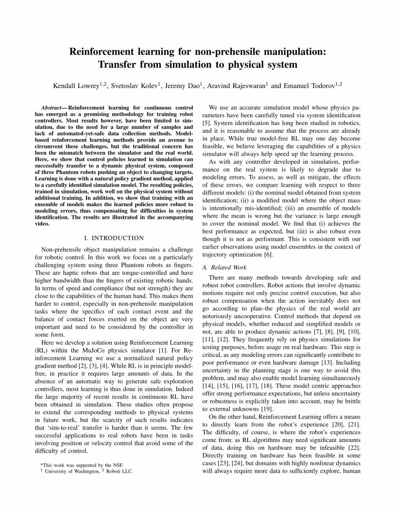
Fig. 1. Learning curve of our linear/affine policy. We show here the curvefor the policy trained with the correct mass as a representative curve.

We implemented our RL code and interfaced with the Mu-JoCo simulator with the Julia programming language [39].The built-in multi-processing and multi-node capabilities ofJulia facilitated this distributed algorithm’s performance; weare able to train a linear policy on this task in less than 3minutes on a 4 node cluster with Intel i7-3930k processors.

Algorithm 1 Distributed Natural Policy Gradient1: Initialize policy parameters to θ02: for k = 1 to K do3: Distribute Policy and Value function parameters.4: for w = 1 to Nworkers do5: Collect trajectories {τ (1), . . . τ (N)} by rolling out

the stochastic policy π(·; θk).6: Compute ∇θ log π(at|st; θk) for each (s, a) pair

along trajectories sampled in iteration k.7: Compute advantages Aπk based on trajectories in

iteration k and approximate value function V πk−1.8: Compute policy gradient according to eq. (2).9: Compute the Fisher matrix (4).

10: Return Fisher Matrix, gradient, and value functionparameters to central server.

11: end for12: Average Fisher Matrix gradient, and perform gradient

ascent (5)13: Update parameters of value function.14: end for

IV. HARDWARE AND PHYSICS SIMULATION

A. System Overview

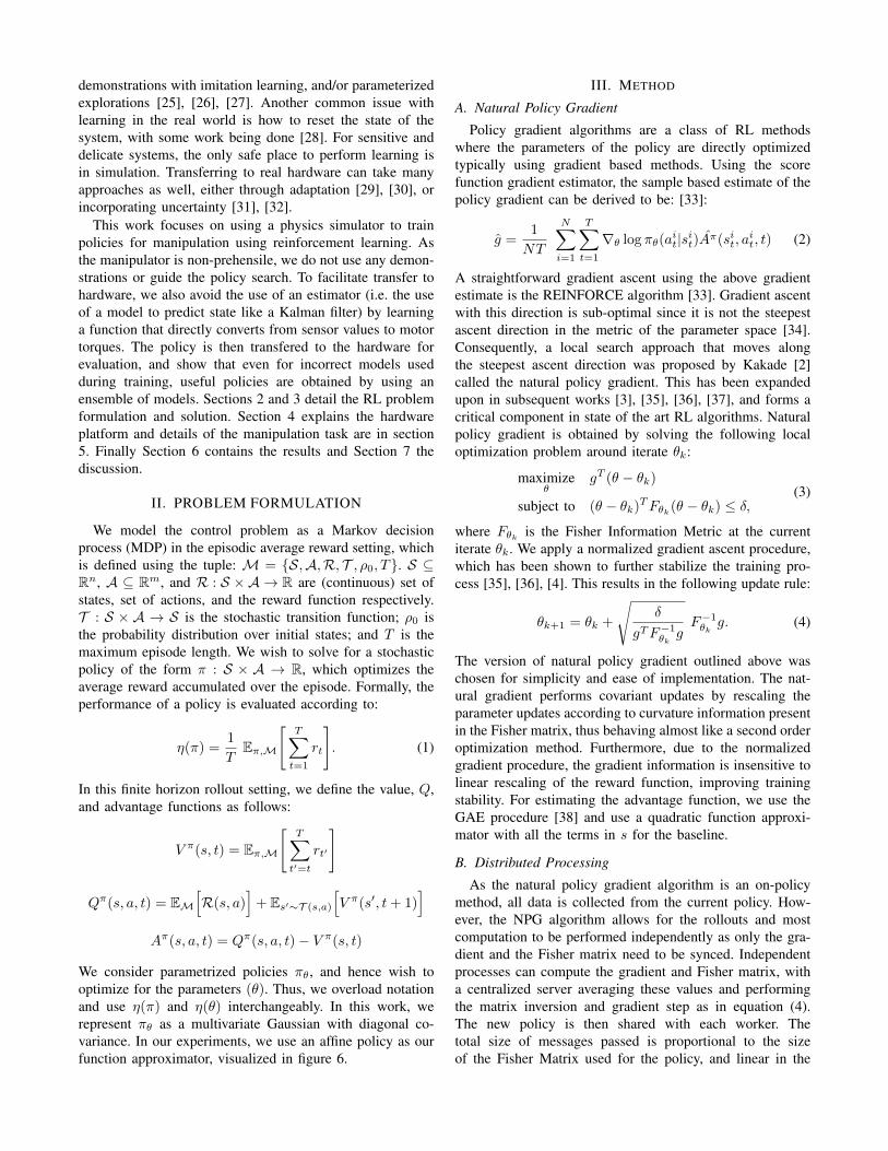
We use our Phantom Manipulation Platform as our hard-ware testbed. It consists of three Phantom Haptic Devices,

Fig. 2. Phantom Manipulation Platform.

each acting as a robotic finger. Each haptic device is a 3-DOF cable driven system shown in figure 2. The actuation isdone with Maxon motors (Model RE 25 #118743), three perPhantom. Despite the low gear reduction ratio, they are ableto achieve 8.5N instantaneous force and 0.6N continuousforce at the middle of their range of motion, with very lowfriction for the entire range of motion.

The three robots are coupled together to act as onemanipulator. Each robot’s end effector was equipped witha silicon covered fingertip to enable friction and reliablegrasping of objects. The softness of the silicon coatingwas an additional challenge in both contact modeling androbust policy learning. For this work, we had the robotsmanipulating a 3D printed cylinder with a height of 14cmand diameter of 11cm, and a mass of 0.34kg.

The soft contacts, combined with the direct torque controland high power-to-weight ratio–leading to high acceleration–make this platform particularly difficult to control. Systemswith more mass and natural damping in their joints naturallymove more slowly and smoothly; this is not the case here.Being able to operate in this space, however, allows for thepotential for high performance, dynamic manipulation, andthe benefits that come with torque based control. However,this requires that we operate our robot controller at 2kHz tosuccessfully close the loop.

B. Sensing

As we wish to learn control policies that map from obser-vations to controls, the choice of observations are critical tosuccessful learning. Each Phantom is equipped with 3 opticalencoders at a resolution of 5K steps per radian. We use a low-pass filter to compute the joint velocities. We also rely on aVicon motion capture system, which gives us position data at240Hz for the object we are manipulating. While being quiteprecise (0.1mm error), the overall accuracy is significantlyworse (< 1mm) due, in part, to imperfect object models andcamera calibrations. While the Phantoms’ position sensors

are noiseless, they often have small biases due to imperfectcalibration. One Phantom robot is equipped with an ATINano17 3-axis force/torque sensor. This data is not usedduring training or in any learned controller, but used as ameans of hardware / simulation comparison described ina later section. The entire system is simulated for policytraining in the MuJoCo physics engine [1].

In total, our control policy has an observational input of36 dimensions with 9 actuator outputs– the 9 positions and9 velocities of the Phantoms are converted to 15 positionsand 15 velocities for modeling purposes due to the parallellinkages. We additionally use 3 positions for both the ma-nipulated object and the tracked goal, with 9 outputs for the3 actuators per Phantom. Velocity observations are not usedfor the object as this would require state estimation that wehave deliberately avoided.

C. System Identification

System identification of model parameters was performedin our prior work [5], but modeling errors are difficult toeliminate completely. For system ID we collected variousbehaviors with the robots, ranging from effector motion infree space to infer intrinsic robot parameters, to manipulationexamples such as touching, pushing and sliding betweenthe end effector and the object to infer contact parameters.The resulting data is fed into the joint system ID and stateestimation optimization procedure. As explained in [5], stateestimation is needed when doing system ID in order toeliminate the small amounts of noise and biases that oursensors produce.

The recorded behaviors are represented as a list of sensorreadings S = {s1, s2, . . . , sn} and motor torques U ={u1, u2, . . . , un}. State estimation means finding a trajectoryof states Q = {q1, q2, . . . , qn}. Each state is a vector qi =(θ1, . . . , θk′ , x, y, z, qw, qx, qy, qz), representing joint anglesand object position. We also perform system ID which isfinding the set of parameters P, which include coefficients offriction, contact softness, damping coefficients, link inertiasand others. We then pose system ID and estimation jointproblem as the following optimization problem:

minP,Q

∑i=1...n

‖τi − ui‖∗1 +∑i=1...n

‖si − si‖∗2

where τi (predicted control signal) and si (predicted sensoroutputs) are computed by the inverse dynamics generativemodel of MuJoCo: (τi, si) = mjinverse(qi−1, qi, qi+1). Theoptimization problem is solved via Gauss-Newton method[5].

V. TASK & EXPERIMENTS

In this section we first describe the manipulation task usedto evaluate learned policy performance, then describe thepractical considerations involved in using the NPG algorithmin this work. Finally, we describe two experiments evaluat-ing learned policy performance in both simulation and onhardware.

A. Task Description

We use the NPG algorithm to learn a pushing task. Thegoal is to reduce the distance of the object, in this casethe cylinder, to a target position as much as possible. Thismanipulation task requires that contacts can be made andbroken multiple times during a pushing movement. As thereare no state constraints involved in this RL algorithm, wecannot guarantee that the object will reach the target location(the object can be pushed into an un-reachable location). Wefeel that this is an acceptable trade-off if we can achievemore robust control over a wider state space.

For these tasks we model the bases of each Phantom asfixed, arrayed roughly equilateral around the object beingmanipulated–this is to achieve closure around the object. Wedo not enforce a precise location for the bases to make themanipulation tasks more challenging and expect them to shiftduring operation regardless.

B. Training Considerations

Policy training is the process of discovering which actionsthe controller should take in which state to achieve a goodreward score, as such, it has implications for how well-performing the final policy is. Training structured informsthe policy of good behavior, but is contrasted with the timerequired to craft the reward function. In this task’s case, weuse a very simple reward structure. In addition to the primaryreward of reducing the distance between the object and thegoal location, we provide the reward function with terms toreduce the distance between each finger tip and the object.This kind of hint term is common in both reinforcementlearning and trajectory optimization. There is also a controlcost, a, that penalizes using too much torque. The entirereward function at time t is as follows:

Rt(s) = 1−3‖|Oxy−Gxy||−3∑i

||fi −Oxy||−0.1a2 (5)

Where Oxy is the current position on the xy-plane of theobject, Gxy is the goal position, and fi is the Phantom endeffector position.

The initial state of each trajectory rollout is with thePhantom robots at randomized joint positions, deliberatelynot contacting the cylinder object. The cylinder location iskept at the origin on the xy-plane, but the desired goallocation is set to uniformly random point within a circleof 12 cm diameter around the origin. To have more diverseinitializations and to encourage robust policies, new initialstates have a chance of starting at some state from one ofthe previous iteration’s trajectories, provided the previoustrajectory had a high reward. If the initial state was acontinuation of the previous trajectory, the target locationwas again randomized: performing well previously onlygives an initial state, and the policy needs to learn to push theobject to a new goal. This is similar to a procedure outlinedin [40] for training interactive and robust policies.

Finally, to further encourage robust behavior, we varythe location of the base of the Phantom robots by adding

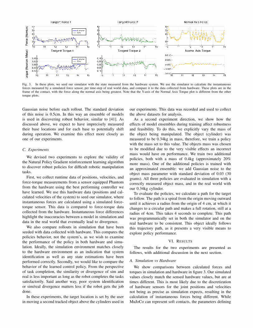
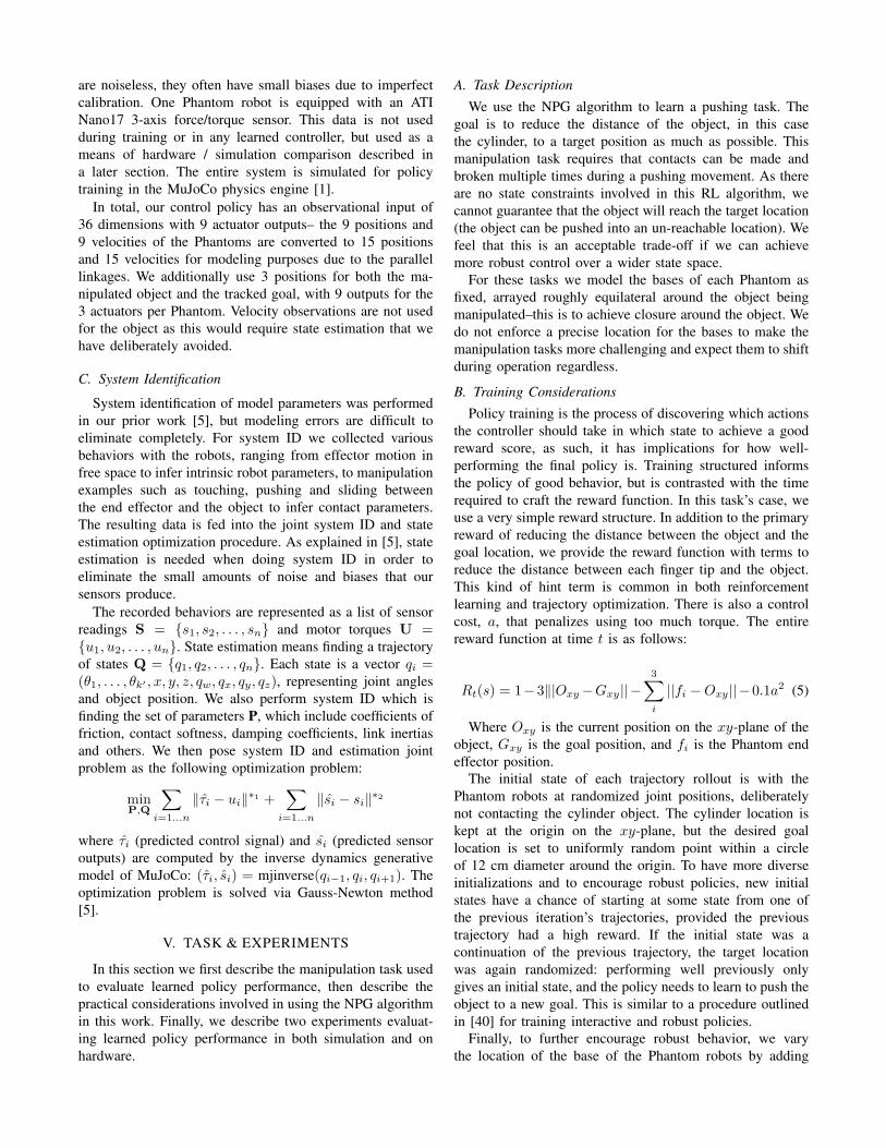
Fig. 3. In these plots, we seed our simulator with the state measured from the hardware system. We use the simulator to calculate the instantaneousforces measured by a simulated force sensor, per time-step of real world data, and compare it to the data collected from hardware. These plots are in theframe of the contact, with the force along the normal axis being greatest. Note that the Y-axis of the Normal Axis Torque plot is different from the othertorque plots.

Gaussian noise before each rollout. The standard deviationof this noise is 0.5cm. In this way an ensemble of modelsis used in discovering robust behavior, similar to [41]. Asdiscussed above, we expect to have imprecisely measuredtheir base locations and for each base to potentially shiftduring operation. We examine this effect more closely asone of our experiments.

C. Experiments

We devised two experiments to explore the validity ofthe Natural Policy Gradient reinforcement learning algorithmto discover robust policies for difficult robotic manipulationtasks.

First, we collect runtime data of positions, velocities, andforce-torque measurements from a sensor equipped Phantomfrom the hardware using the best performing controller wehave learned. We use this hardware data (positions and cal-culated velocities of the system) to seed our simulator, whereinstantaneous forces are calculated using a simulated force-torque sensor. This data is compared to force-torque datacollected from the hardware. Instantaneous force differenceshighlight the inaccuracies between a model in simulation anddata in the real world that eventually lead to divergence.

We also compare rollouts in simulation that have beenseeded with data collected with hardware. This compares thepolicies behavior, not the system’s, as we wish to examinethe performance of the policy in both hardware and simu-lation. Ideally, the simulation environment matches closelyto the hardware environment as an indication that systemidentification as well as any state estimations have beenperformed correctly. Secondly, we would like to compare thebehavior of the learned control policy. From the perspectiveof task completion, the similarity or divergence of sim andreal is less important as long as the robot completes the taskssatisfactorily. Said another way, poor system identificationor sim/real divergence matters less if the robot gets the jobdone.

In these experiments, the target location is set by the userin moving a second tracked object above the cylinders used in

our experiments. This data was recorded and used to collectthe above datasets for analysis.

As a second experiment direction, we show how theeffects of model ensembles during training affect robustnessand feasibility. To do this, we explicitly vary the mass ofthe object being manipulated. The object (cylinder) wasmeasured to be 0.34kg in mass, therefore, we train a policywith the mass set to this value. The objects mass was chosento be modified due to the very visible effects an incorrectmass would have on performance. We train two additionalpolicies, both with a mass of 0.4kg (approximately 20%more mass). One of the additional policies is trained withan approximated ensemble: we add Gaussian noise to theobject mass parameter with standard deviation of 0.03 (30grams). All three policies are evaluated in simulation with acorrectly measured object mass, and in the real world withour 0.34kg cylinder.

To evaluate the policies, we calculate a path for the targetto follow. The path is a spiral from the origin moving outwarduntil it achieves a radius from the origin of 4 cm, at which itchanges to a circular path and makes a full rotation, still at aradius of 4cm. This takes 4 seconds to complete. This pathwas programmatically set in both the simulator and on thereal hardware to be consistent. This object ideally followsthis trajectory path, as it presents a very visible means toexplore policy performance.

VI. RESULTS

The results for the two experiments are presented asfollows, with additional discussion in the next section.

A. Simulation vs Hardware

We show comparisons between calculated forces andtorques in simulation and hardware in figure 3. Our simulatedvalues closely match the sensed hardware values, but are attimes different. This is most likely due to the discretizationof hardware sensors for the joint positions and velocitiesnot being as precise as simulation expects, resulting in thecalculation of instantaneous forces being different. WhileMuJoCo can represent soft contacts, the parameters defining

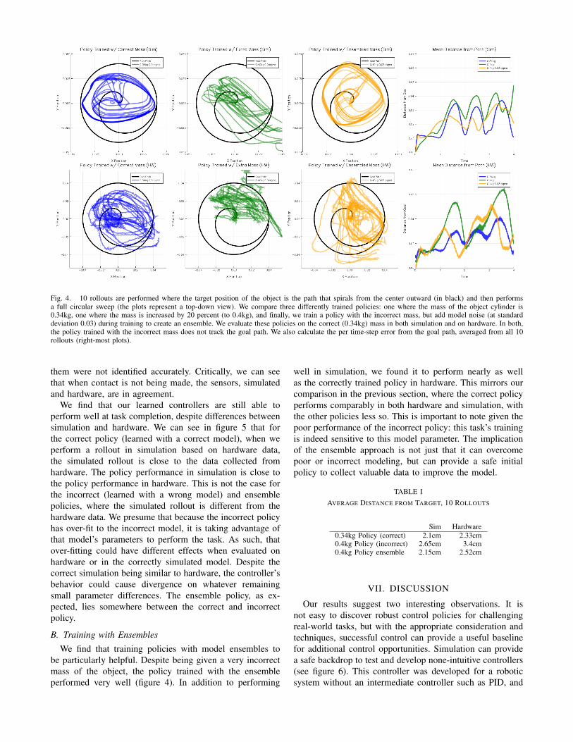
Fig. 4. 10 rollouts are performed where the target position of the object is the path that spirals from the center outward (in black) and then performsa full circular sweep (the plots represent a top-down view). We compare three differently trained policies: one where the mass of the object cylinder is0.34kg, one where the mass is increased by 20 percent (to 0.4kg), and finally, we train a policy with the incorrect mass, but add model noise (at standarddeviation 0.03) during training to create an ensemble. We evaluate these policies on the correct (0.34kg) mass in both simulation and on hardware. In both,the policy trained with the incorrect mass does not track the goal path. We also calculate the per time-step error from the goal path, averaged from all 10rollouts (right-most plots).

them were not identified accurately. Critically, we can seethat when contact is not being made, the sensors, simulatedand hardware, are in agreement.

We find that our learned controllers are still able toperform well at task completion, despite differences betweensimulation and hardware. We can see in figure 5 that forthe correct policy (learned with a correct model), when weperform a rollout in simulation based on hardware data,the simulated rollout is close to the data collected fromhardware. The policy performance in simulation is close tothe policy performance in hardware. This is not the case forthe incorrect (learned with a wrong model) and ensemblepolicies, where the simulated rollout is different from thehardware data. We presume that because the incorrect policyhas over-fit to the incorrect model, it is taking advantage ofthat model’s parameters to perform the task. As such, thatover-fitting could have different effects when evaluated onhardware or in the correctly simulated model. Despite thecorrect simulation being similar to hardware, the controller’sbehavior could cause divergence on whatever remainingsmall parameter differences. The ensemble policy, as ex-pected, lies somewhere between the correct and incorrectpolicy.

B. Training with Ensembles

We find that training policies with model ensembles tobe particularly helpful. Despite being given a very incorrectmass of the object, the policy trained with the ensembleperformed very well (figure 4). In addition to performing

well in simulation, we found it to perform nearly as wellas the correctly trained policy in hardware. This mirrors ourcomparison in the previous section, where the correct policyperforms comparably in both hardware and simulation, withthe other policies less so. This is important to note given thepoor performance of the incorrect policy: this task’s trainingis indeed sensitive to this model parameter. The implicationof the ensemble approach is not just that it can overcomepoor or incorrect modeling, but can provide a safe initialpolicy to collect valuable data to improve the model.

TABLE IAVERAGE DISTANCE FROM TARGET, 10 ROLLOUTS

Sim Hardware0.34kg Policy (correct) 2.1cm 2.33cm0.4kg Policy (incorrect) 2.65cm 3.4cm0.4kg Policy ensemble 2.15cm 2.52cm

VII. DISCUSSION

Our results suggest two interesting observations. It isnot easy to discover robust control policies for challengingreal-world tasks, but with the appropriate consideration andtechniques, successful control can provide a useful baselinefor additional control opportunities. Simulation can providea safe backdrop to test and develop none-intuitive controllers(see figure 6). This controller was developed for a roboticsystem without an intermediate controller such as PID, and

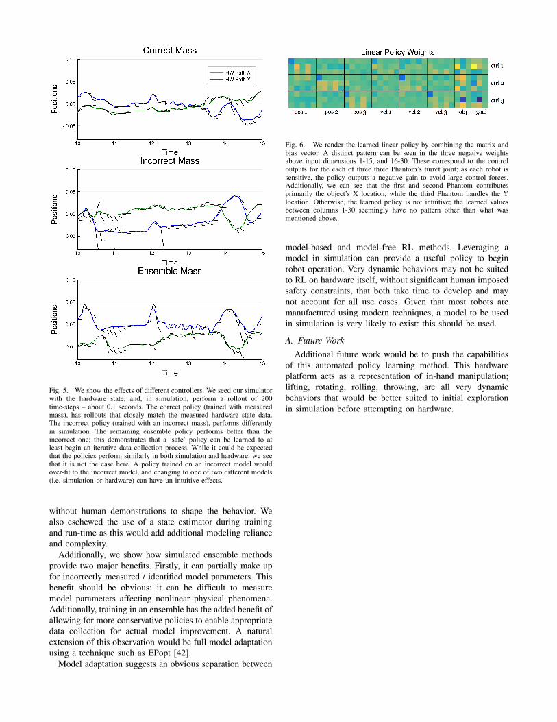
Fig. 5. We show the effects of different controllers. We seed our simulatorwith the hardware state, and, in simulation, perform a rollout of 200time-steps – about 0.1 seconds. The correct policy (trained with measuredmass), has rollouts that closely match the measured hardware state data.The incorrect policy (trained with an incorrect mass), performs differentlyin simulation. The remaining ensemble policy performs better than theincorrect one; this demonstrates that a ’safe’ policy can be learned to atleast begin an iterative data collection process. While it could be expectedthat the policies perform similarly in both simulation and hardware, we seethat it is not the case here. A policy trained on an incorrect model wouldover-fit to the incorrect model, and changing to one of two different models(i.e. simulation or hardware) can have un-intuitive effects.

without human demonstrations to shape the behavior. Wealso eschewed the use of a state estimator during trainingand run-time as this would add additional modeling relianceand complexity.

Additionally, we show how simulated ensemble methodsprovide two major benefits. Firstly, it can partially make upfor incorrectly measured / identified model parameters. Thisbenefit should be obvious: it can be difficult to measuremodel parameters affecting nonlinear physical phenomena.Additionally, training in an ensemble has the added benefit ofallowing for more conservative policies to enable appropriatedata collection for actual model improvement. A naturalextension of this observation would be full model adaptationusing a technique such as EPopt [42].

Model adaptation suggests an obvious separation between

Fig. 6. We render the learned linear policy by combining the matrix andbias vector. A distinct pattern can be seen in the three negative weightsabove input dimensions 1-15, and 16-30. These correspond to the controloutputs for the each of three three Phantom’s turret joint; as each robot issensitive, the policy outputs a negative gain to avoid large control forces.Additionally, we can see that the first and second Phantom contributesprimarily the object’s X location, while the third Phantom handles the Ylocation. Otherwise, the learned policy is not intuitive; the learned valuesbetween columns 1-30 seemingly have no pattern other than what wasmentioned above.

model-based and model-free RL methods. Leveraging amodel in simulation can provide a useful policy to beginrobot operation. Very dynamic behaviors may not be suitedto RL on hardware itself, without significant human imposedsafety constraints, that both take time to develop and maynot account for all use cases. Given that most robots aremanufactured using modern techniques, a model to be usedin simulation is very likely to exist: this should be used.

A. Future Work

Additional future work would be to push the capabilitiesof this automated policy learning method. This hardwareplatform acts as a representation of in-hand manipulation;lifting, rotating, rolling, throwing, are all very dynamicbehaviors that would be better suited to initial explorationin simulation before attempting on hardware.

REFERENCES

[1] E. Todorov, T. Erez, and Y. Tassa, “Mujoco: A physics engine formodel-based control,” pp. 5026–5033, 2012.

[2] S. Kakade, “A natural policy gradient,” in NIPS, 2001.[3] J. Peters and S. Schaal, “Natural actor-critic,” Neurocomputing,

vol. 71, pp. 1180–1190, 2007.[4] A. Rajeswaran, K. Lowrey, E. Todorov, and S. Kakade, “Towards

generalization and simplicity in continuous control,” arXiv preprintarXiv:1703.02660, 2017.

[5] S. Kolev and E. Todorov, “Physically consistent state estimation andsystem identification for contacts,” in Humanoid Robots (Humanoids),2015 IEEE-RAS 15th International Conference on. IEEE, 2015, pp.1036–1043.

[6] I. Mordatch, K. Lowrey, and E.Todorov, “Ensemble-CIO: Full-bodydynamic motion planning that transfers to physical humanoids,” inIROS, 2015.

[7] Y. Tassa, T. Erez, and E. Todorov, “Synthesis and stabilization of com-plex behaviors through online trajectory optimization,” in IntelligentRobots and Systems (IROS), 2012 IEEE/RSJ International Conferenceon. IEEE, 2012, pp. 4906–4913.

[8] I. Mordatch, E. Todorov, and Z. Popovic, “Discovery of complexbehaviors through contact-invariant optimization,” ACM Transactionson Graphics (TOG), vol. 31, no. 4, p. 43, 2012.

[9] Y. Tassa, N. Mansard, and E. Todorov, “Control-limited differentialdynamic programming,” in Robotics and Automation (ICRA), 2014IEEE International Conference on. IEEE, 2014, pp. 1168–1175.

[10] S. Feng, E. Whitman, X. Xinjilefu, and C. G. Atkeson, “Optimization-based full body control for the darpa robotics challenge,” Journal ofField Robotics, vol. 32, no. 2, pp. 293–312, 2015.

[11] J. Koenemann, A. Del Prete, Y. Tassa, E. Todorov, O. Stasse, M. Ben-newitz, and N. Mansard, “Whole-body model-predictive control ap-plied to the hrp-2 humanoid,” in Intelligent Robots and Systems(IROS), 2015 IEEE/RSJ International Conference on. IEEE, 2015,pp. 3346–3351.

[12] M. Raibert, K. Blankespoor, G. Nelson, and R. Playter, “Bigdog, therough-terrain quadruped robot,” IFAC Proceedings Volumes, vol. 41,no. 2, pp. 10 822–10 825, 2008.

[13] D. Nguyen-Tuong and J. Peters, “Model learning for robot control: asurvey,” Cognitive processing, vol. 12, no. 4, pp. 319–340, 2011.

[14] I. Mordatch, N. Mishra, C. Eppner, and P. Abbeel, “Combiningmodel-based policy search with online model learning for control ofphysical humanoids,” in Robotics and Automation (ICRA), 2016 IEEEInternational Conference on. IEEE, 2016, pp. 242–248.

[15] Y. Pan and E. A. Theodorou, “Data-driven differential dynamic pro-gramming using gaussian processes,” in American Control Conference(ACC), 2015. IEEE, 2015, pp. 4467–4472.

[16] J. M. Wang, D. J. Fleet, and A. Hertzmann, “Optimizing walking con-trollers for uncertain inputs and environments,” in ACM Transactionson Graphics (TOG), vol. 29, no. 4. ACM, 2010, p. 73.

[17] G. Lee, S. S. Srinivasa, and M. T. Mason, “Gp-ilqg: Data-drivenrobust optimal control for uncertain nonlinear dynamical systems,”arXiv preprint arXiv:1705.05344, 2017.

[18] S. Ross and J. A. Bagnell, “Agnostic system identification for model-based reinforcement learning,” arXiv preprint arXiv:1203.1007, 2012.

[19] M. Johnson, B. Shrewsbury, S. Bertrand, T. Wu, D. Duran, M. Floyd,P. Abeles, D. Stephen, N. Mertins, A. Lesman, et al., “Team ihmc’slessons learned from the darpa robotics challenge trials,” Journal ofField Robotics, vol. 32, no. 2, pp. 192–208, 2015.

[20] J. Peters, S. Vijayakumar, and S. Schaal, “Reinforcement learning forhumanoid robotics,” in Proceedings of the third IEEE-RAS interna-tional conference on humanoid robots, 2003, pp. 1–20.

[21] L. P. Kaelbling, M. L. Littman, and A. W. Moore, “Reinforcementlearning: A survey,” Journal of artificial intelligence research, vol. 4,pp. 237–285, 1996.

[22] J. Kober, J. A. Bagnell, and J. Peters, “Reinforcement learning inrobotics: A survey,” The International Journal of Robotics Research,vol. 32, no. 11, pp. 1238–1274, 2013.

[23] S. Gu, E. Holly, T. Lillicrap, and S. Levine, “Deep reinforcementlearning for robotic manipulation with asynchronous off-policy up-dates,” in Robotics and Automation (ICRA), 2017 IEEE InternationalConference on. IEEE, 2017, pp. 3389–3396.

[24] M. Deisenroth and C. E. Rasmussen, “Pilco: A model-based anddata-efficient approach to policy search,” in Proceedings of the 28thInternational Conference on machine learning (ICML-11), 2011, pp.465–472.

[25] Y. Chebotar, M. Kalakrishnan, A. Yahya, A. Li, S. Schaal, andS. Levine, “Path integral guided policy search,” in Robotics andAutomation (ICRA), 2017 IEEE International Conference on. IEEE,2017, pp. 3381–3388.

[26] A. Yahya, A. Li, M. Kalakrishnan, Y. Chebotar, and S. Levine, “Col-lective robot reinforcement learning with distributed asynchronousguided policy search,” arXiv preprint arXiv:1610.00673, 2016.

[27] J. Kober and J. R. Peters, “Policy search for motor primitives inrobotics,” in Advances in neural information processing systems, 2009,pp. 849–856.

[28] W. Montgomery, A. Ajay, C. Finn, P. Abbeel, and S. Levine, “Reset-free guided policy search: efficient deep reinforcement learning withstochastic initial states,” in Robotics and Automation (ICRA), 2017IEEE International Conference on. IEEE, 2017, pp. 3373–3380.

[29] I. Menache, S. Mannor, and N. Shimkin, “Basis function adaptationin temporal difference reinforcement learning,” Annals of OperationsResearch, vol. 134, no. 1, pp. 215–238, 2005.

[30] S. Barrett, M. E. Taylor, and P. Stone, “Transfer learning for reinforce-ment learning on a physical robot,” in Ninth International Conferenceon Autonomous Agents and Multiagent Systems-Adaptive LearningAgents Workshop (AAMAS-ALA), 2010.

[31] M. Cutler, T. J. Walsh, and J. P. How, “Reinforcement learning withmulti-fidelity simulators,” in Robotics and Automation (ICRA), 2014IEEE International Conference on. IEEE, 2014, pp. 3888–3895.

[32] P. Abbeel, M. Quigley, and A. Y. Ng, “Using inaccurate modelsin reinforcement learning,” in Proceedings of the 23rd internationalconference on Machine learning. ACM, 2006, pp. 1–8.

[33] R. J. Williams, “Simple statistical gradient-following algorithms forconnectionist reinforcement learning,” Machine Learning, vol. 8, no. 3,pp. 229–256, 1992.

[34] S. Amari, “Natural gradient works efficiently in learning,” NeuralComputation, vol. 10, pp. 251–276, 1998.

[35] J. Peters, “Machine learning of motor skills for robotics,” PhDDissertation, University of Southern California, 2007.

[36] J. Schulman, S. Levine, P. Moritz, M. Jordan, and P. Abbeel, “Trustregion policy optimization,” in ICML, 2015.

[37] J. Schulman, F. Wolski, P. Dhariwal, A. Radford, and O. Klimov,“Proximal policy optimization algorithms,” arXiv preprintarXiv:1707.06347, 2017.

[38] J. Schulman, P. Moritz, S. Levine, M. Jordan, and P. Abbeel, “High-dimensional continuous control using generalized advantage estima-tion,” in ICLR, 2016.

[39] J. Bezanson, S. Karpinski, V. B. Shah, and A. Edelman, “Julia:A fast dynamic language for technical computing,” arXiv preprintarXiv:1209.5145, 2012.

[40] I. Mordatch, K. Lowrey, G. Andrew, Z. Popovic, and E. V. Todorov,“Interactive control of diverse complex characters with neural net-works,” in Advances in Neural Information Processing Systems, 2015,pp. 3132–3140.

[41] I. Mordatch, K. Lowrey, and E. Todorov, “Ensemble-cio: Full-bodydynamic motion planning that transfers to physical humanoids,” inIntelligent Robots and Systems (IROS), 2015 IEEE/RSJ InternationalConference on. IEEE, 2015, pp. 5307–5314.

[42] A. Rajeswaran, S. Ghotra, S. Levine, and B. Ravindran, “Epopt:Learning robust neural network policies using model ensembles,”arXiv preprint arXiv:1610.01283, 2016.