REINFORCED GRASS ON INNER DIKE SLOPES

Student: Silvia Hinostroza Garcia

Date:

December 2007

αφ

γ φ

δ

ΔΔ

ΔΔ

τ

τ

Student S.Hinostroza Garcia Student number 1294407 Email silviamilagros@yahoo.com Faculty Civil Engineering Variant Hydraulic Engineering Specialization Hydraulic Structures Comitee: Prof. dr. ir. M.J.F. Stive TUDelft Ir. H.J. Verhagen TUDelft Dr. ir.A.Fraaij TUDelft Dr. ir. G.J.C.M. Hoffmans RWS DWW

1

Abstract This thesis shows a set of equations that define the micro-stability and macro-stability of reinforced grass revetments with geosynthetics on inner dike slope during an overtopping event. At micro-stability level, it has been analyzed that the equilibrium in a soil particle using the criterion of incipient motion of soil particle. The forces in normal direction to water flow are considered the most important to keep in equilibrium the soil particles of the reinforced grass revetment. As unstable forces are considered: Lift force, this force can be defined in function of depth-averaged relative turbulence intensity and averaged-velocity (Hoffmans’ Model, 2006). Likewise, the averaged-velocity can be defined in function of concentration factor of stems, bent vegetation height and vegetation height (Carollo’s Model, 2005) As stable forces are taken account: Friction force due to cohesion stress, the cohesion forces produced by root and geosynthetic in the soil are assumed in the same direction of the water flow and they cause a frictional forces in the normal direction of water flow when the particle tend to detach. Also, gravity force, as it is referred to submerged weight of soil particle. The stability equation of a soil particle of reinforced grass revetment is deduced from the application of the equilibrium between these forces; it means unstable forces must be equal or less than stable forces. At macro-stability level, it has been analyzed the acting forces on reinforced grass revetment during an overtopping event has been applied to the equilibrium in the system. The diagram of free body of reinforced grass revetment is divided in two wedges and identified like active and passive wedges (Koerner’s model 1991). The wedge located at top of the slope exerts an active function in the system that means it tends to push away the soil of the revetment so that is in the toe of the slope. The other wedge located at toe exerts a passive function that consist to hold the active wedge giving equilibrium to the system. The forces taken account in the diagram of free body of both wedges are: the weight of the soil, the shear force of the water, the cohesion forces produced by cohesive soil, roots and geosynthetics, reactive forces located in the failure plane and pressure forces between the passive and active wedges. To define the stability of the system, the safety factor is introduced in the friction angles of different soils and soil-geosyntethic besides in the cohesion produced by root and geosynthetics. The polygon method is applied in the forces acting on each wedge and it is deduced in a quadratic equation in function of safety factor. A safety factor higher than one defines a stable system. The geosynthetic analyzed are the geogrid and geocell. Unlike geogrid for the geocell an additional force is considered and this is the shear force which is generated in the contact between geocell wall and soil and it is in normal direction of the surface. This additional force is independent of the geocell tension; it means the geocell does not need to be in tension to help the stability of the system. In the case of geogrid could not be affirm the same. With much analysis of micro-stability as macro-stability of the system, the cohesive forces produced by roots and geosynthetics are important. In this thesis is described in brief mathematical models, based on equation’s coulomb, which defined these cohesions. The cohesion produced by root in the soil is calculated using the simple root perpendicular model (Model of Wu et al, 1979). The additional cohesion produced by the geosynthetic uses the model of Jewell, 1980, to be calculated. Both cohesion models are based on the tension stress of the root or geosynthetic located inside of the soil layer produce shear stress in this layer. The shear stress could be in any plane but it is used the failure plane. This shear stress in the failure plane is composed of two components, one of the component is the projection of tension stress in the failure plane and the other is the friction stress produced by the normal component to the failure plane of tension. The tension of roots and geosynthetics are important in both cohesion models. The tension of root is easily to obtain from laboratory.

2

In this thesis the tension in the geosynthetics is calculated in the same way proposed by Koerner’s method with some modifications. The tension produced in the geosynthetic is the differences between the internal pressures that exert the active wedgen and passive wedge of a grass revetment unstable during an overtopping event. This way how to estimate the tension is valid for geogrid and geocell. However it is described in a model in the case of the grass revetment is stable and the instability is produced when the water is flowing in the slope. The geosynthetic does not have any tension when the system is stable but when the water is running down on the slope generates an angular deformation in some geosynthetic like is the case of the geogrid. This angular deformation is in the plane along of the slope and it produces tensional stress in the geogrid generating cohesion into the soil. The criterion used to describe this tension is similar to the theory of beams lied down on elastic foundation. The geogrid is sensible to this deformation because its thickness is quite low. Geosynthetic like geocell has higher thickness so they are not sensible to this angular deformation so in this thesis is presented other alternative to define the shear stress in the failure plane. The criterion of Jewell is not easy applicable since the failure plane is assumed parallel to the surface of slope. Assuming that the longitudinals and unit deformations that are produced in the reinforced grass revetment are equals in the soil and in the geocell, the failure shear stress could be defined using the equation of Mohr. A mathematical equation using the mentioned criterions is shown in this thesis. Besides this model can include the cohesion produced by root and define the failure shear stress of a grass revetment reinforced with geocell. A set of equations containing many variables are presented in this thesis so it is recommend to make a detailed analysis of relevant and irrelevant parameters in subsequent studies to simplify these models and make them more viable in the test of laboratories.

3

Table of Contents LIST OF FIGURES LIST OF TABLES LIST OF SYMBOLS 1. INTRODUCTION

1.1. BACKGROUND 1.2. PROBLEM DEFINITION 1.3. OBJECTIVES OF THE STUDY 1.4. METHODOLOGY

2. GRASS REVETMENTS ON INNER SLOPES 2.1. TYPICAL CONFIGURATION 2.2. INNER SLOPES OF DUCTH SEA DIKES 2.3. TURF 2.4. ROOTS INCREASE RESISTANCE OF SOIL 2.5. BOTANICAL CHARACTERISTICS 2.6. MECHANICAL CHARACTERISTICS OF THE ROOTS

2.6.1. LIMIT OF ROOT GROWTH 2.6.2. DENSITY OF ROOTS 2.6.3. DIAMETER OF ROOTS 2.6.4. TENSILE STRESS OF ROOTS 2.6.5. THE PULLOUT FORCE OF ROOTS 2.6.6. SOIL-ROOT MATRIX COHESION 2.6.7. ANGLE OF SHEAR DISTORTION OF ROOTS 2.6.8. ANGLE OF INTERNAL FRICTION ( )φ OR ( )'φ 2.6.9. ROOT AREA RATIO

2.7. MANAGEMENT PROCEDURE 3. HYDRAULIC ASPECTS

3.1. HYDRAULIC LOADS IN SEA DIKES 3.2. WAVE OVERTOPPING DESIGN DISCHARGE 3.3. GROUNDWATER FLOW LOAD THROUGH DIKE 3.4. HYDRAULIC BEHAVIOUR OF THE SUBMERGED GRASS 3.5. OVERTOPPING FLOW LOADS

3.5.1. SHEAR WATER FORCE 3.5.2. DRAG WATER FORCE 3.5.3. LIFT FORCE 3.5.4. COHESIVE FORCES

4. GEOTECHNICAL ASPECTS 4.1. CLAY AND SAND AMONG TURF

4.1.1. THE MECHANICAL BEHAVIOUR OF SOIL UNDER STRESSES 4.1.2. SHEAR STRESS OF SANDY CLAY 4.1.3. RESIDUAL SHEAR STRESS 4.1.4. SHALLOW SURFACE SLIP

4.2. SHEAR STRESS IN THE SOIL-ROOT MATRIX 4.2.1. THE SIMPLE PERPENDICULAR ROOT MODEL 4.2.2. THE FIBER BUNDLE MODEL IN ROOT

4.3. BEHAVIOR OF REINFORCED SOILS UNDER STRESSES 4.3.1. REINFORCED SOIL UNDER VERTICAL STRESSES 4.3.2. REINFORCED SOIL UNDER HORIZONTAL STRESSES

4.4. SHEAR STRESS MODEL IN THE REINFORCED SOIL 4.5. SHEAR STRESS IN THE REINFORCED-ROOT-SOIL MATRIX

5. GEOSYNTHETIC REINFORCEMENT AT SLOPES 5.1. GEOGRID CHARACTERISTICS 5.2. PULL-OUT STRESS OF GEOGRIDS 5.3. SHEAR STRESS OR COHESION DUE TO GEOGRIDS INTO THE SOIL 5.4. GEOCELLS CHARACTERISTICS 5.5. VERTICAL AND HORIZONTAL STRESS IN THE GEOCELLS 5.6. SHEAR STRESS OR COHESION DUE TO GEOCELLS INTO THE SOIL 5.7. STABILITY OF COVER SOIL ON GEOMEMBRANE LINED SLOPES

4

5.8. REQUIRED TENSILE STRENGTH OF GEOGRID REINFORCEMENT OF COVER SOIL ON AN GEOMEMBRANE

5.9. STABILITY OF GRASS REVETMENT DURING AN OVERTOPPING EVENT USING KOERNER METHOD

5.10. TENSILE STRENGTH OF GEOSYNTHETIC REINFORCEMENT OF GRASS REVETMENT

6. SLOPE STABILITY ANALYSES OF REINFORCED GRASS 6.1. MICRO-STABILITY OF OUTER GRAINS ON REINFORCED GRASS REVETMENT 6.2. MACRO-STABILITY OF REINFORCED GRASS REVETMENT 6.3. LOADS PRESENT IN THE STATIC MODEL 6.4. STATIC MODEL REINFORCED GRASS REVETMENT WITH PRETENSED

GEOGRID DURING AN OVERTOPPING EVENT 6.5. STATIC MODEL REINFORCED GRASS REVETMENT WITH PRETENSED

GEOCELLS DURING OVERTOPPING MODEL 6.6. COHESION DUE TO GEOSYNTHETIC INTO THE SOIL-REINFORCED-GRASS

MATRIX OF THE REVETMENT 7. CONCLUSIONS AND RECOMMENDATIONS

7.1. ADITIONAL ROOT COHESION IN THE SOIL 7.2. ADITIONAL GEOCELL COHESION IN THE SOIL 7.3. ADITIONAL GEOSYNTHETIC COHESION IN UNSTABLE GRASS REVETMENTS 7.4. ADITIONAL COHESION IN STABLE GRASS REVETMENTS DUE TO TENSION

IN GEOGRID GENERATED DURING AN OVERTOPPING EVENT 7.5. MICRO-STABILITY METHOD 7.6. MACRO-STABILITY METHOD 7.7. GENERAL RECOMMENDATIONS

REFERENCES APENDIX I: CALCULATION MODEL OF WAVE OVERTOPPING DESIGN DISCHARGE APPENDIX II: TENSILE STRENGTH OF DIFERENT PLANTS APENDIX III: COEFFICIENT ACCORDING USDA

5

LIST OF FIGURES Fig. 1.1-1: The waves run over the inner slope originating erosion of grass layer Fig. 1.1-2: Successful grass growth in a synthetic mat (Source: http:// www.hoofmark.co.uk/Golpla/ GolplaBrochure.html) Fig. 1.1-3: Reinforced grass revetments with a netting (Source: http:// www.nagreen.com/resources/literature/TF-04-05.pdf) Fig. 1.1-4: Bi-axial and Uni-axial Geogrid (Source: http:// www.geofabrics.com.au/geogrid.htm) Fig. 1.1-5:Geocells with perforated and non-perforated sides (Source: http:// www.alcoa.com/alcoa_consumer_products/prestogeo/en/solutions/geoweb_specifications.asp) Fig. 1.1-6: Geonet (Source: http:// www.china-synergy.org/geogrid.htm) Fig. 1.1-7: Geomat (Source: http:// www.colbond-geosynthetics.com) Fig. 2.1-1: Composition of clay layer with grass cover (Source: H.J. Verhagen-dikes (20-04-00)) Fig. 2.2-1: Sea dike of Friesland (Source: Msc Thesis of Wilbert Van de Bos, 2006) Fig. 2.4-1: The roots compress the loose soil Fig. 2.5-1: Some typical grass plants (Source: Hewlett, 1987, CIRIA, Report 116) Fig. 2.6.2-1: Density of roots versus depth based on investigation of Hähne, 1991(Source: Ms thesis of Vavrina, 2006) Fig. 2.6.2-2: A rough calculation of root density Fig. 2.6.2-3: Graphs of root length density and root weight density from Dutch dike strata samples (Source: Sprangers H, 1999) Fig. 2.6.4-1: Relation between diameter and tensile stress of Vetiver roots (Source: Msc Thesis of Maaskant, 2005) Fig. 2.6.5-1: Graph showing estimated pullout versus breaking forces for River birch roots in a soil with strength of 6KPa (Source: Pollen N, Simon A, 2005) Fig. 2.6.6-1: Simple schematic of shear testing Fig. 2.6.7-1: Hypothetical deformation of the root in the shear zone Fig. 2.6.8-1: Angle of repose or angle of friction of a pile of grains Fig. 2.6.9-1: Graphs of root area ratio calculated from drρ and drγ of Dutch dike strata samples tested by Sprangers (Source: Msc Thesis of Young M, 2005) Fig. 2.7-1: Grass growth according management grassland applied (Source: Hans Sprangers,1994) Fig. 3.1-1: Overtopping process including main failure mechanisms (Source: http://awww.rug.ac.be/opticrest/html/abstracttask35.pdf) Fig. 3.2-1: Wave overtopping event at a sea dike (Source: http:// sun1.rrzn.uni-hannover.de/fzk/e6/e6_1/icce2002_failure.pdf) Fig. 3.3-1: Force on inner slope due to porous flow Fig. 3.4-1: Geometrical features of vegetation under water ((Source: Carollo F.G., 2005) Fig. 3.4-2: Typical velocity profile of a submerged flexible vegetation. Diagram u-y in which “u” is local velocity and “y” is the height of water from the bottom (Source: Carollo F.G., 2005) Fig. 3.5-1: Shear Forces acting on a loose grain and on reinforced grass revetments Fig. 4.1-1: Some differences between clay soil and sandy soil Fig. 4.1.1-1: Forces acting on the particle of soil Fig. 4.1.1-2: Shear stress in soil Fig. 4.1.1-3: Phenomenon of dilatation and compaction in sand soil Fig. 4.1.3-1: Frictional force in the contact plane between geosynthetic and soil of a reinforced revetment Fig. 4.1.4-1: Equilibrium forces parallels to slope at reinforced grass revetment Fig. 4.2.1-1: Root crossing the soil shear zone and stressed in tension Fig. 4.2.1-2: Root Cohesion for a 3mm-diameter root with different RAR and Tension Stress Fig. 4.3.1-1: Soil element under vertical stress with lateral compression due to adjacent soil Fig. 4.3.1-2: Reinforced soil element under vertical stress is confined by horizontal stress in the reinforcement Fig. 4.3.2-1: Soil element under shear stress with lateral compression due to adjacent soil and shear distortion angle Fig. 4.3.2-2: Non-rigid reinforced soil element under shear stress Fig. 4.3.2-3: Rigid reinforced soil element under shear stress Fig. 4.4-1: Rigid reinforced soil element under shear stress Fig. 4.4-2: Rigid reinforced soil element under shear stress Fig. 4.4-3: Rigid reinforced soil element under shear stress Fig. 5.1-1: Geogrid Unidirectional (Source: http://www.tenax.net/geosynthetics/products/tenax_tt.htm) Fig. 5.1-2: Geogrid Bi-directional (Source: http://www.tenax.net/geosynthetics/products/tenax_lbo_geogrids.htm) Fig. 5.2-1: Pull-out stress of geogrid (Source: Diagram from Koerner, 1994) Fig. 5.3-1: Distortion of geogrid due to shear stress of water Fig. 5.3-2: Beam lies down on elastic foundation under load of distributed moment Fig. 5.4-1: Variable expansion of the geocell

6

Fig. 5.5-1: Bearing capacity failure mechanisms of sand with geocell (Source: Diagram from Koerner, 1994) Fig. 5.5-1: Pressure pore and active earth pressure acting on wall of geocell Fig. 5.6-1: Unit deformation of the soil with geocell Fig. 5.7-1: Pasive and active wedge with forces involves in free diagram body of a cross-section of cover soil on a geomembrane (Source: Koerner & Hwu, 1991) Fig. 5.7-2: Diagram of free body for passive and active wedge of cover soil on a geomembrane (Source: Koerner & Hwu, 1991) Fig. 5.8-1: Geogrid reinforcement of cover soil on geomembrane (Source: Koerner & Hwu, 1991) Fig. 5.9-1: Forces acting on active and passive wedges of grass revetment during an overtopping event Fig. 5.9-2: Forces acting on passive wedges of grass revetment during an overtopping event Fig. 5.9-3: Forces acting on active wedge of grass revetment during an overtopping event Fig. 5.10-1 : Geosynthetic reinforcement of grass revetment during an overtopping event Fig. 6.1-1: Incipient motion of soil particle of reinforced grass revetment Fig. 6.2-1: Forces acting on slice of grass revetment due to an overtopping event on inner slope Fig. 6.3-1: Forces acting on active and passive wedges of reinforced grass revetment due to an overtopping event on inner slope Fig. 6.4-1: Forces acting on active and passive wedges of reinforced grass revetment with geogrid Fig. 6.4-2: Forces acting on passive wedge of reinforced grass revetment with geogrid Fig. 6.4-3: Forces acting on active wedge of reinforced grass revetment with geogrid Fig. 6.5-1: Forces acting on active and passive wedges of reinforced grass revetment with geocell Fig. 6.5-2: Forces acting on passive wedge of reinforced grass revetment with geocell Fig. 6.5-3: Forces acting on active wedge of reinforced grass revetment with geocell

7

LIST OF TABLES Table 2.1-1: Characteristics of layer to compose of grass revetments Table 2.2-1: Typical outer and inner slopes in the different dikes of the Netherlands Table 2.4-2: Erosion rates at grass layer Table 2.5-1: Plant community on Dutch sea dikes Table 2.5-2: Plant community on Dutch sea dikes Table 2.6.3-1: Mean root diameter of some species of plants Table 2.6.4-1: Tensile stress of roots of some species of plants Table 2.6.6-1: Additional cohesion in the soil due to roots according different investigators Table 2.7-1: Categories of grass cover quality according management grassland Table 3.1-1: Maximum velocities of erosion in good grass cover of inner slopes Table 3.2-1: Maximum overtopping discharge over inner slopes Table 3.4-1: Description of the velocity profile diagram for flexible vegetation according to Carollo, 2005. Table 3.4-2: Recalibrated Coefficient of Kouwen’s flow resistance law Table 3.4-3: Coefficient of Carollo et al’s flow resistance law Table 3.5.1-1: Values of soil roughness in function of 75DTable 3.5.1-2: The permissible soil shear stress ( )soilp,τ according to U. S. Department of

transportation Table 3.5.3-1: The lift force values replacing values of Carollo et al, Hoffmans and U.S. Department Transportation

( LF )Table 4.1-1: Classification of soil into the turf if it has the maximum recommended quantity of sand Table 4.1.2-1: Characteristics of different soils Table 4.4-1: Ultimate tensile strength per unit width of geosynthetics Table 5.1-1: Young’s modulus of polyester fibres coated with polyethylene Table 5.1-2: Young’s modulus of some polymers Table 5.4-1: Specification of three-dimensional geocell confinement of Geoweb System Table 5.9-1: Forces acting on the passive and active wedge of grass revetment during an overtopping event Table 6.4-1: Forces acting on the passive and active wedge of reinforced grass revetment during an overtopping event Table 6.5-1: Forces acting on the passive and active wedge of reinforced grass revetment during an overtopping event

8

LIST OF SYMBOLS The following is a list of the more important symbols in this thesis. A : Area parallels to surface of root-soil matrix (m2)

rA : Total cross-sectional area of the roots (mm2)

cA : Exposed surface area of a particle of soil (mm2)

⊥gA : Area perpendicular to slope of geosynthetic (m2)

sA : Area of the soil element (m2)

RA : Total cross sectional area of roots in the area A (m)

A : Area parallels to surface of root-soil matrix (m2)

fc : Shear coefficients (----)

d : Particle diameter (m)

75De

: Soil size where 75% of the material is finer (mm) : Void ratio (----)

g : Acceleration gravity (m/s2)

h : Depth of water (m)

I : Moment of Inertia (m4) I : Bed Slope (----)

*u : Bed shear velocity (m/s)

u : Velocity averaged over the vertical or the cross section (m/s)

soilp,τ : Soil permissible shear stress (N/m2)

ψ : Dimensionless mobility parameter (----)

PI : Plasticity index (----) 'fτ : Shear stress on the failure plane f-f (kN/m2)

'fσ : Effective stress on the failure plane f-f μσσ −= ff ' (kN/m2)

μ : Pore water pressure (kN/m2)

'φ : Friction angle based on effective stresses ( 0 )

'c : Cohesion based on effective stresses. (kN/m2)

tensiongeogridF − : Total pullout strength (kN)

SLR : Longitudinal rib shear strength (m)

STR : Transverse rib shear strength (m)

bTR : Transverse rib bearing strength (m)

oq : Bearing capacity (kN/m2) τ : Shear stress (kN/m2) τ : Shear stress acting on geosynthetic between contacts of (kN/m2) Soil and geosynthetic : Passive pressure lateral earth pressure (kN/m2) pP

wρ : Water density (kg/ m3)

sρ : Mass soil density (kg/ m3)

wγ : Water specific weight (kN/m3) g : Acceleration gravity (m/s2)

i : Hydraulic gradient (----) φ : Angle of repose or internal friction ( 0 ) α : Angle of slope ( 0 )

9

pθ : Angle between horizontal and streamline at slope face ( 0 )

pF : Pullout force (kPa)

'τ : Maximum tangential stress (kPa)

rootL : Root length (m)

rootd : Root diameter (m)

rootCΔ : Root additional cohesive strength (kPa)

θ : Root shear distortion angle ( 0 ) x : Horizontal deformation of shear zone (m) z : Depth of shear zone (m)

ria : Cross sectional area of root-i (mm2)

drρ : Dry root mass density (g/dm3)

drγ : Dry root unit weight (kN/dm3) g : Acceleration gravity (m/s2)

ra : Average root cross section area (mm2)

rLq

: Root length density (m/dm3) : Overtopping discharge (l/s)

D : Thickness of revetment (m)

vv IE : bending stiffness (N-m2)

vv IME : bending stiffness (N-m2)

vE : Longitudinal elasticity modulus of the grass (N/m2)

vI : Inertia moment of grass cross section (m4)

M : Vegetation concentration per unit concentration ( 2

2

//dmstemdmstem

)

oM : Unit vegetation concentration (1 stem/dm2)

h : Depth of water (m)

sh : Bent vegetation height (m) *u : Shear velocity (m/s) *cu

u : Critical shear velocity (m/s)

: Bed velocity (m/s) V : Mean flow velocity (m/s)

vH : Vegetation height in the absence of flow (m)

0C : Coefficient of Kouwen’s flow resistance law (----)

1C : Coefficient of Kouwen’s flow resistance law (----)

1a : Coefficient of Carollo et al’s flow resistance law (----)

2a : Coefficient of Carollo et al’s flow resistance law (----)

3a : Coefficient of Carollo et al’s flow resistance law (----)

d : Particle diameter (m)

75D : Soil size where 75% of the material is finer (mm) ν : Kinematic viscocity (m2/s) τ : Shear stress (kN/m2)

bτ : Design shear stress (N/m2)

cτ : Critical shear stress (kN/m2)

10

eτ : Effective shear stress (N/m2)

dτ : Design shear stress (N/m2)

fC : Grass cover factor (----)

nC : Grass roughness coefficient (----)

sn : Soil grain roughness (----) n : Overall lining roughness (----)

soilp,τ : Permissible soil shear stress (N/m2)

vp ,τ : Permissible shear stress on the vegetative lining (N/m2)

DC : Drag coefficient (----)

DF : Drag water force (N)

maxp : Difference between the positive and negative pressure peaks (N/m2)

LF : Lift force (N)

oU : Average-velocity (m/s)

V : Averaged-velocity (m/s)

or : averaged relative turbulence intensity (----)

oc : Coefficient (----)

sP : Percentage of fines (----)

crτ : Critical bed shear stress (N/m2)

shieldsc,τ : Critical bed-shear stress according to Shields (N/m2)

2α : Coefficient (----)

3α : Coefficient (----)

E : Modulus of elasticity (N/m2)

soilE : Elastic modulus of soil (N/m2)

icgeosynthetE : Elastic modulus of geosynthetic (N/m2)

n'σ : Normal effective stress (kN/m2)

p'τ : Peak shear strength (kN/m2)

gs /τ : Shear stress between soil and geosynthetic (kN/m2)

r'τ : Residual shear stress (kN/m2)

sW : Weight of soil (kN)

r'ϕ : Residual angle ( 0 )

rτ : Parallel shear stress to surface produced by root (kN/m2)

rσ : Perpendicular stress to surface produced by root (kN/m2)

RT : Average tensile stress (kN/m2)

irT : Tensile strength of roots in size class I (kN/m2)

ira : Section area of root in size class I (m2)

irn : Number of roots in size class I (----)

hσ : Horizontal stress caused by lateral compression (kN/m2)

1ε : Relative displacement

2ε : Relative displacement

11

gT : Tensional stress in the reinforcement (kN/m2)

θ : Angle between geosynthetic and shearing direction or ( 0 ) Distortion angle of geosynthetic-root-soil matrix

'maxφ : Maximum angle of shear resistance of soil ( 0 )

T : Reinforced tensile force (N)

icgeosynthetCΔ : Geosynthetic additional cohesive strength (kPa) 'sφ : Friction angle of the soil ( 0 )

GGB : Minimum width of geogrid aperture (m)

50D : Average particle size (m)

rt : Thickness of geosynthetic (mm)

rE : Young’s modulus of polyester fibres (kN/m2) ω : Angle of rotation in soil-root-geogrid ( 0 )

0M : Distributed moment (kN-m/m)

M : Moment produced in the geogrid

geogridI : Inertia of geogrid (m4)

'b : Sum of all widths of tranverse rib of geogrid (m) in a width of mb 1= e : Thickness of geogrid (m)

cω : Rotation angle at point in the geogrid lied down (rad) c on slope due to distributed moment

cM : Moment at point c in the geogrid lied down on (kN-m) Slope due to distributed moment L : Longitude of the dike slope (m)

cT : Tensional force in the geogrid at point c (kN)

k : Modulus of foundation per unit width (kN/m2)

gA : Sectional area of geogrid (m2)

geocellτ : Shear strength between geocell wall and soil (kN/m2)

contained within it.

hσ : Average horizontal force within the geocell (kN/m2) p : Applied vertical pressure, for a unit width

aK : Coefficient of active earth pressure (----)

δ : Angle of shearing resistance (friction angle) between ( 0 ) soil and the cell wall material

1σ : Total pressure at the upper thickness of geocell (kN/m2)

2σ : Total pressure at the lowest thickness of geocell (kN/m2)

ε : Unit deformation of the geocell in the direction of (----) ε : Unit deformation of geocell in the direction of tensional (----) force

geoT : Tension force in the geocell (kN)

12

1. INTRODUCTION

1.1. BACKGROUND Along the Dutch coast line are located a system of dikes and dunes which protected against storm surges with a frequency of once every ten thousand years (Herman G. Wind). The most of these dikes were constructed with core of sand and some of clay. This core is covered by a strong layer to increase its withstand against any kind of failure. The outer slope (seaward) of the sea dike has a hard revetment to support the wave actions. The dike crest and the inner slope (landward) of the sea dike have in the average a 1.0m of clay thick with a grass layer. When the storm surges are over the crest level of the sea dikes, the waves run over the inner slope originating hydraulic loadings, steady overflow or a low-exceedance wave overtopping events, which damage the grass layer. This damage can occurs in the following ways: removal of any loose vegetation, scour of soil from roots, loss of individual plants, roll up of soil-root mat, shallow surface slip and net uplift from excessive seepage flow (CIRIA, report 116). Once the soil layer is exposed, the vulnerability of dike increases due to the erosion process is more quickly. This no means that the alternative of using a grass cover must be turned down but rather the necessity of look for new alternatives that increase the strength of grass revetments must be done. The most of dutch sea dikes has a inner slope of grass revetment, some preliminary studies shows that is cheaper to reinforce the grass layer than raising the crest of the sea dikes (Com Coast WP3).

Fig. 1.1-1: The waves run over the inner slope originating erosion of grass layer The grass layer is composed by a sward above the ground which reduces the velocity of the flow and originates turbulence at the same time, a turf adjacent to surface where composite soil-root mat is formed and a layer under the turf where a root structure anchors the composite soil-root mat to substrate. Consequently the base of the soil-root mat must be considered as a zone of potential weakness. (CIRIA, report 116). This plain grass can be enhance its engineering functions with the use of some sort of reinforcement. Some of those functions must be:

• Control of soil-root mat erosion: Resist soil migration, movement and extraction caused by negative hydraulic pressure and impact forces of turbulent flow.

• Local erosion: improvement in lateral continuity between grass plants avoid individual plants dislodge from soil-root mat.

13

Fig. 1.1-2: Successful grass growth in a synthetic mat (Source: http://

www.hoofmark.co.uk/Golpla/GolplaBrochure.html)

Reinforced a grass layer means the use of tensile properties of a geosynthetic material to resist stresses or deformations in geotechnical structures as inner slopes of dutch sea dikes. The material available in the market to reinforce grass can be divide into two groups: geotextile and concrete. Obviouly the geotextile system is cheaper. Thus the study of this thesis will be concentrated in the materials of geotextile. These geotextile materials are either woven fabrics, meshes or mats. At the same time they are subdivided in two-dimensional, three-dimensional open and three-dimensional filled. To evaluate which material should be used as grass reinforcement is necessary to consider:

• Drainage: The perpendicular and parallel drainage to inner slope must be guaranteed since inadequate drainage will reduce grass growth therefore the strength of soil-root mat.

• Pore size: It is needed a large one due to the grass can penetrate through this material. (Pilarczyk)

• Layer of soil-root mat beneath the grass reinforcement: it is needed since the roots need to prolongate and to penetrate between 12mm–15mm in order to thrive and to anchor.

• Durability: The most material used as reinforcement has synthetic components like polypropylene, nylon, polyethylene, polyester, etc. so prolonged sunlight causes to decay in strength and performance. Excessive UV rays destroy the synthetic molecular bonds.

• Thermic properties: During hot weather plastic is an insulator the roots can not have problems to growth or to keep alive in contrast concrete.

• Gradient: To prevent lateral movement of the root-soil mat.

Fig. 1.1-3: Reinforced grass revetments with a netting

(Source: http:// www.nagreen.com/resources/literature/TF-04-05.pdf) However for analysis of this thesis the most important is the mechanical properties like tensile strength and to find a relation that can define how the presence of geosynthetics get better the cohesion properties of the soil.

14

A previous study made by Akkerman (ComCoast WP3 report) suggests some selected mashes which withstand slope inner without remove the present grass revetment along the

identified

Most of them are made of polypropylene, polyethylene and polyester. It is recommended to apply over flat surfaces with good grass cover. See Fig.1.1-4

Dutch coast line. Innoving new methods of installations compares to traditional ones. They two principal systems:

• Two dimensional mesh (Geogrid): The geogrid is a geosynthetic material consisting of connected parallel set of intersecting ribs (transversal and longitudinal) with open spaces or apertures (10-100mm). Where the direction of major stresses are known uni-axial geogrid is used and where the direction are random bi-axial geogrid must be applied.

Fig. 1.1-4: Bi-axial and Uni-axial Geogrid (Source: http:// www.geofabrics.com.au/geogrid.htm)

• Three dimensional mesh (Geocells): The geocells are geosynthetic material consisting of cellular confinement with a height. They are made from multiples strips of strong polyethylene sheets which are welding together along their thick so that when the strips are separated they form an open honeycomb configuratio

n.They confine the soil layer within cellular structure so improve granular soil shear strength. It works in uneven surfaces with poor grass. See Fig.1.1-5.

at. A difference of previously mentioned products its application over the present rass revetments is complicate however in this thesis they will be studied like a reinforced

ure is formed when the ribs are opened. The extrusion process does not strech the molecules of polymer so the tensile strength is relatively low. See Fig.1.1-6

Fig. 1.1-5:Geocells with perforated a n-perforated sides (Source: http:// www.alcoa.com/alcoa_consumer_products/prestogeo/en/solutions/geoweb_specifications.asp)

There are other materials which can be used like reinforced grass revetments like Geonet and Geom

nd no

gmaterial.

• Geonet: It is a geosynthetic material formed by a continuous extrusion of connected parallel sets of polymeric ribs at acute angles to one another. The netlike configuration or continuous net struct

15

• Geomat or 3-D mats: It is a three-dimensional geosynthetic net mades of bonded

filaments.

Fig. 1.1-6: Geonet (Source: http:// www.china-synergy.org/geogrid.htm)

Fig. 1.1-7: Geomat (Source: http:// www.colbond-geosynthetics.com)

Although all these materials made of polypropylene, polyethylene or/and polyester processed using different techniques get better the tension properties of the layer of grass avoiding the soil/root mat erosion is necessary to understand how, when and why the failure in the layer of soil/root/reinforcement due to overtopping can occur since there is not a lot information and

s will make an analysis for predicts failure of the reinforced

ghly erodible) and finally collapse. To change whole rass revetment is costly so it is better to lay down geosynthetic that get stronger the layer of

se are not too muchso this esis propose mathematical model that describe the increment of cohesion in the soil due to

of grass layer that allow the right application and dimension of inforced material taking in account some material has to be applied without remove the

rass layer laid in situ.

test respect to this yield. This thesigrass layer.

1.2. PROBLEM DEFINITION As it was mentioned above, the current protection of the most of inner slopes against erosion of the Dutch sea embankments is the grass layer. The moderate to good closed grass layer can not withstand average overtopping discharge higher than 10 l/s per m width (TAW, 1997) so apply technologies that reduce detachment of soil particles of soil/root mat is necessary. Any kind of failure as rolling up the soil must be avoiding since the sea embankments is in high risk to loose material (sand is higsand and clay seeded with grass. The two and three dimensional mesh makes strong the grass layer due to increase the cohesion of soil like the roots make. Thus the soil with root and geosynthetics is more resistant to erosion. Theories that explain how the cohesion increathtensional forces in the geosynthetic under some assumptions. Actually in the market there are lot products which are offered available to fulfill with this reinforced requirements. However there are not so much tests, knowledge and experience respect to understanding why grass is failing under overtopping conditions which can serve as reference. It is necessary to base on a theoretical investigation to try understand the mechanism of failures reg

16

1.3. OBJECTIVES OF THE STUDY The objective of this thesis is to produce a set of equations that help to define the stability of reinforced grass revetment on inner slope during an overtopping event. Thus a compilation of previous theorical investigation about the description the mechanisms of grass tail failures were made in this thesis. Starting from these investigations that describe the failure of grass revetments, to find possible strengthening solutions. The strengthening solutions involve to

nalize two dimensional geosynthetic like geogrid and three dimensional geosynthetic like eocell.

is used.

used. - The water shear stress that takes accounts the turbulence intensity. The model of

this information, new models that allow describing the micro-stability of a soil

nd the

to move away the passive wedge. The desequilibrium between the pressures of these wedges makes

s down on elastic foundation were introduced to calculate this tension but these models are only referencial and they are not considered in the equations of stability of this thesis.

ag

1.4. METHODOLOGY The methodology applied in this thesis was firstly based on the compilation of models that describe:

- The stability of a soil particle located on the based of channel. The model of Booij (1998) is used.

- The stability of a slope covers with cohesive soil. The model of Koerner and Wu (1991) is used.

- The cohesion of the soil revetment when this has roots. The model of Wu et al (1979) and O’Loughlin (1982)

- The cohesion of the soil revetment due to presence of geosynthetics. The model of Jewell (1980) is used.

- The average-velocity definition when the slope of the channel is cover with grass. The model of Carollo (2005) is

Hoffmans (2006) is used. Starting fromparticle of a reinforced grass revetment and macro-stability of this revetment have been developed.

- Respect to the micro-stability, the model of destabilize forces were redefined. For instance the lift force in this thesis takes account the grass’ characteristics aturbulence of flow. The stabilize forces are in function of cohesion produced by roots and geosynthetics. The frictional angle of the soil is important in this analysis.

- Respect to the macro-stability, based on Koerner’s model, the reinforced grass revetment was divided in two wedges. The active wedge tends

unstable the system. The water shear stress was considered too. Each theory was analyzed and it was realized that the tension of geosynthetics lied down in the soil revetment is an important factor to calculate the additional cohesion in the soil according Jewell model. However additional models using the theory of beams lie

17

2. GRASS REVETMENTS ON INNER SLOPES In this chapter in brief important characteristics of the Grass revetment will be mentioned. Questions as How is it defined? What is the shape of the seadikes which protects? What is the turf or sod? Why roots increase the resistance of soil? What is the typical botanical species? How the management procedure plays out in the process of strengthening of grass? These questions are answered based on previous studies and tests.

2.1. TYPICAL CONFIGURATION Grass cover is the most nature, common and cheap revetments on the slopes. According to TAW 1999, grass revetment is grassland vegetation rooted in soil and its composition is showed in Fig. 2.1-1. From this figure It can say that the grass revetment is composed of:

• Herbage layer: This visible layer is formed by sward and stubbles. The sward height typical is almost 10cm during winter and it has flowers too. The stubbles are short stems of 2cm in average and they make up part of upper turf (layer on which grass is growing). There are some loose roots here too forming a layer between 1mm and 3mm.

• Clay layer: This invisible layer is divided by two layers called topsoil and subsoil. The topsoil, a mixture of clay and roots of grass and organic layer, contents part of beneath turf (layer of grass-earth on which roots grow). This turf layer has a high root density when it is wet its elastic properties increase and it is porous too due to the clay which form this layer is influenced by climate, generating shrink and swell, and activities of soil fauna, some animals dig holes or channels in soil layers. The root density decrease with the depth. The first depth between 5mm and 50mm has 55% of the roots so it has high permeability and the subsequent layer between 50mm and 150mm reduce the permeability and the presence of the roots. The topsoil has a substrate layer too on which the presence of roots is almost scarce. The subsoil entirely formed by clay is stiff when dry or plastic in moist conditions and less is permeable. The resistance erosion of this layer is lesser than the topsoil layer.

Many reports about this topic mention the sod layer, which it is just turf, is the upper and densely rooted part. It forms an irregular bed structure which takes the strain to erosion. (TAW 1999).

Fig 2.1-1: Composition of clay layer with grass cover (Source: H.J. Verhagen-dikes (20-04-00)

In the Table 2.1-1, it is showed a summary of the characteristics of layers which compose the grass revetments.

18

TABLE 2.1-1: Characteristics of layer to compose of grass revetments

Principal

layers Sub-layers Components Thickness Properties

Sward Herbage Herbage layer Stubble Upper turf 20 mm Loose roots (1mm-3mm)*

Beneath turf 5mm - 150 mm 55% of roots (5mm – 50mm)* Less roots (50mm – 150mm)* Topsoil

Substrate 150 mm – 500 mm Scarce roots Clay layer

Subsoil Substrate 500 mm – 1500 mm No presence of roots only clay *Source: MSc Thesis of Wilbert van de Bos, 2006 The principal function of the grass cover on the inner slopes of the sea dikes is protection against erosion caused by overtopping discharge no higher than 1 l/s per m or by seepages in some cases. This protection depends of the root system of the turf or sod.

2.2. INNER SLOPES OF DUCTH SEA DIKES The most sea dikes in the Netherlands have an outer slope covered of stones or asphalt principally those located on Zeeland, Friesland and Groningen. The inner slope is covered of grass layer which varies in quality, density and strength. The minimum width of the crest is 3m and the height varies respect to the location in average is 10m. The overtopping rate can be reduced if the outer slope increases its roughness. The core of the dike is composed by sand or clay. The dikes with sand-core are covered on a clay layer. Ones of clay-core which are older has been strengthened with an additional body of sand at landward and covered on clay layer too, sometimes this clay-core is forming only the berms. The clay layer waterproofs the core of the dike avoiding the flow through pores and the generation of pore pressure. The typical range of slopes of the different type of Dutch dikes is showed in the Table 2.2-1.

Table 2.2-1: Typical outer and inner slopes in the different dikes of the Netherlands Characteristic slope of dikes in the Netherlands

( horizontal : vertical ) Type of dike Outer Slope Inner Slope

River 1:2 – 1:3 1:2 – 1:3 Lake Flatter than 1:3 1:2 – 1:2.5 Sea Flatter than 1:4 1:2.5 – 1:3

Source: MSc Thesis of Wilbert van de Bos, 2006

Fig 2.2-1: Sea dike of Friesland (Source: Msc Thesis of Wilbert Van de Bos, 2006)

19

2.3. TURF Many believe that the erosion resistance of the grass cover is due to a layer of grass leaves and stems (herbage layer). However some tests prove that this resistance depends on the structure of roots and soils which constitute “the turf or sod” with thickness is between 5 – 15 cm. The factors which influence this resistance are the depth and density of root network, tensile strength of roots and clay granular composition. (Hans Sprangers,1999). This means turfs with a low root density have a low erosion resistance and vice versa. • Soil in turf is composed by small and large particles in which interspaces there are pores

and roots. The diameter of these particles is between 0.002 – 5 mm. The smaller particles join amongst themselves by different mechanisms to constitute the larger size. See Table2.3-1. So particles lower than 20 μm agglutinate because of ionic charges of clays. Matter organic from bacterial origin and roots, cementing materials and fine network of roots are factors in the adherence mechanisms of particles, they give more stability to soil against clean out of the hydraulic load . Cementing materials depend on chemical processes in the area of the roots, so resistance of grass depends on ageing of turf. The particle stability is affected by seasonal changes so at the end of winter there are low particles higher than 2mm than at the end of summer. This is due to presence of fungi and bacterial population of roots which influence cohesion.

Table 2.3-1: Mechanism of adherence of soil in turf related to diameter of particles

Aggregates diameter of turf (mm) Mechanism of adherence

< 0.002 Coagulation 0.002 – 0.02 Bacterial origin 0.02 – 0.25 Roots and cementation

0.25 – 5 Fine network of roots, fungal hyphae, penetrates aggregates Source: Hans Sprangers, 1999. • Roots grow vertically and horizontally. The vertical growth (tap root system) is made by

the most prominent root or roots to anchor in the topsoil and subsoil. This backbone of fibrous material increases tensile strength of grass layer controlling its sliding. The horizontal or the lateral growth is carried out by roots called rhizomes (fibrous root system). These are lower tensile strength but more effective in reducing surface of erosion. Additionally the interlinking, enclosure and penetration the particles form a soil-root matrix. This matrix increases the shear strength of the soil as well as elasticity. Erosion test of turf prove that those with high density of roots have finer particles of soil than those with low density (Van Essen, 1994).

2.4. ROOTS INCREASE RESISTANCE OF SOIL

In order for the roots to grow in the soil, they have to beat the mechanical resistance which this porous medium imposes on them. This is achieved by penetrating existing pours and cracks of a higher diameter than the roots or deforming the structure of medium. The roots are available to adapt their form and movement to soil obstacles. That is deform or change the soil whether fracturing or/and compressing. Root growth depends of pressure of turgencia. This is the pressure that exerts the content of the cell against the membrane. The root growth when surpasses the rigidity of cellular walls and of the soil solids. The maximum pressure in axial and radial direction is shown in the Table 2.4-1.

Table 2.4-1: Maximum pressure of roots at axial and radial direction Direction of the root Maximum pressure of roots in the soil

(MPa) Axial 0.7 -1.3

Radial 0.4 – 0.6 Source: Daniel L. Martino, 2003. If the mechanical resistance of soil is higher than these limits it is expected that there is not growth. However the presence of a continuous system of big pours can reduce the resistance of soil matrix allowing the growth.

20

This growth depends directly of axial pressure but the radials strengths also influence it since they widen the smaller pours to the diameter of the roots. They cause cracks in the soil located in front of root tip and they increase the total strength applied at axial direction when the thickness or transversal section increases. This also increases the friction between the root and soil getting better anchorage to exert the axial strength. It is known is that loose soils are more prone to erosion than those are compacted. It is the compact grade or package of soil particles that establish its sensibility to erosion. The embedded roots through the soil porous cause compression of the soil during its radial expansion. The compression is located around the roots. The volume occupied by the roots is compensated with a decrease of higher pour volume. These are the reasons why the presence of roots in the soil makes that this compression a better resistance against erosion. Some tests have been done to calculate the erosion rates of turf and it has been found that a higher density of roots in the turf has better erosion resistance. This means that the top layer of the turf is more compressed by presence of many roots than the lower layer. The granular composition and the amount and size of clay aggregates also influence in this resistance. See Table 2.4-2.

Table 2.4-2: Erosion rates at grass layer

Depth (cm)

Percentage of the total amount of roots

(%)

Erosion Rates (cm/hour)

0 – 6 65 0.1 – 0.2 6 – 15 20 2 – 3

15 – 50 15 > 10 Source: Hans Sprangers, 1999.

Fig 2.4-1: The roots compress the loose soil

2.5. BOTANICAL CHARACTERISTICS The plant communities more common on Dutch sea dikes are shown in Table 2.6. These varieties depend on type of management applied chiefly. The soil type and habitat factors in situ influence too however they are not determining.

21

TABLE 2.5-1: Plant community on Dutch sea dikes

Plant community Characteristic species On what sea dikes?

Species-rich Oat-grass hay meadow

Hedge vetch, Meadow fescue, Rough hawksbeard, Smooth bedstraw/False baby’s breath, Tall buttercup

Not fertilised area

Crested dog’s tail pasture

Smooth bedstraw, Timothy grass, Cinquefoil, Daisy, Self-heal, Small hawbit, Jacob’s cross, Crested dog’s tail, Kingcup, Ground ivy

Not fertilised area

Species-poor variant of crested dog’s tail pasture

------------ Sandy areas on sea dikes

Oat-grass hay meadow with edge species

Leafy spurge, wild marjoram, cross-leaved bedstraw, hairy ragwort, rampion bellflower.

Sea dikes in Zeeland

Species-poor Rye grass meadow

English, rye grass, Daisy, Wild geranium Fertilised area

Fallow pasture with tall herbs

Fertilised area

Source: Erosion Resistance of Grassland as dike covering, TAW 1997 The turf of Oat-grass hay meadow and Crested dog’s tail pasture is closed so this allows to conform a strong soil-root matrix and these plant communities have a good behaviour against erosion (TAW 1997). The Fig. 2.5-1 shows some species of grass plants like Rye grass, Red fescue and Meadow grass.

Fig 2.5-1: Some typical grass plants (Source: Hewlett, 1987, CIRIA, Report 116)

The following Table shows all types of grasses communities used as cover in the different slopes of Dutch river and sea dikes and its behaviour against erosion (TAW 1997).

22

Table 2.5-2: Plant community on Dutch sea dikes

Grassland Type Indicative number

of species per 25 m2

Erosion resistance of the sod

Ecological value

Grassland management

Streamside valley grassland 30 Very good Very high 1 to 2 x haying,

unfertilised False oat meadow with edge species 27 Good Very high Irregular haying,

unfertilised False oat meadow diverse 32 Very good Very high 1 to 2 x haying,

unfertilised False oat meadow, non-diverse 13 Moderate Low Haying, fertilized

Rough meadowland 8 – 20 Poor Low Haying, heavily fertilized, or mulch mowing

Crested dog’s-tail grass, diverse 36 Very good High Pasturing,

unfertilized Crested dog’s-tail grass, non-diverse 15 Good Low Pasturing, lightly

fertilized Bluegrass-rye grass meadow 12 – 18 Moderate Low Pasturing, heavily

fertilized Source: Erosion Resistance of Grassland as dike covering, TAW 1997 Laying grass cover is executed in the following procedure: first, placing the clay and sowing and seeding grass and herbs this lasts 1 or 2 years, and second, control of herbs germination, in this phase it is tried to generate a closed vegetation by knitting together of separate plants, this lasts between 3-5 years. It could be said that the total development of grass cover takes between 4-7 years.

2.6. MECHANICAL CHARACTERISTICS OF THE ROOTS

2.6.1. LIMIT OF ROOT GROWTH The limit of root growth is the depth on the turf where properties the roots have influence as a reinforcement in the soil-root matrix. Some definition was used by Hähne (1999), who calculate that is 12.8 cm in an intensive cultivated soil with a minimum of shear strength equal to 10.1 KPa (Vavrina, 2006).

)( gt

gt

2.6.2. DENSITY OF ROOTS The density of the roots depends on the type of sward, location and composition of soil. For this reason take account about what kind of sward we are referring. But example according to Ford (2003) who made some tests with the Pampa Grass or Cortaderia Jubata used a density of 62 root/m2 and according to Hänne (1991) shows density between 20,000 to 80,000 roots/m2 but he does not specify the kind of sward and the average diameter of the roots. The Fig. 2.5 shows the density of the roots related with the depth of topsoil prepared by Hänne (1991), however it is not specified the type of sward.

23

Fig 2.6.2-1: Density of roots versus depth based on investigation of Hähne, 1991

(Source: Ms thesis of Vavrina, 2006)

For to have an idea about density of root, we can see that the general grass here has an average diameter of 3mm and if we have an area which section of 2cm x 2cm it is logical to find almost 24 roots in average. It means 60000 roots/m2. See the Fig.2.6.2-2.

Fig 2.6.2-2: A rough calculation of root density

Comparing this value with the graph about root density of Hähne (1991) it is not unreal to say that this quantity reduces with the depth of the turf so the root density should be assumed 15000 roots/m2 approximately for a topsoil layer higher than 0.30m. It is almost 10% the area of the roots in one square meter. There is not information about tests made in the Dutch dike revetments to estimated root densities, however there are data of root weigh density and root length density (Sprangers, H, 1999). In the Fig.2.6.2-3 it is shown some information from some samples of roots taken from Dutch dikes with different treatment of fertilization.

24

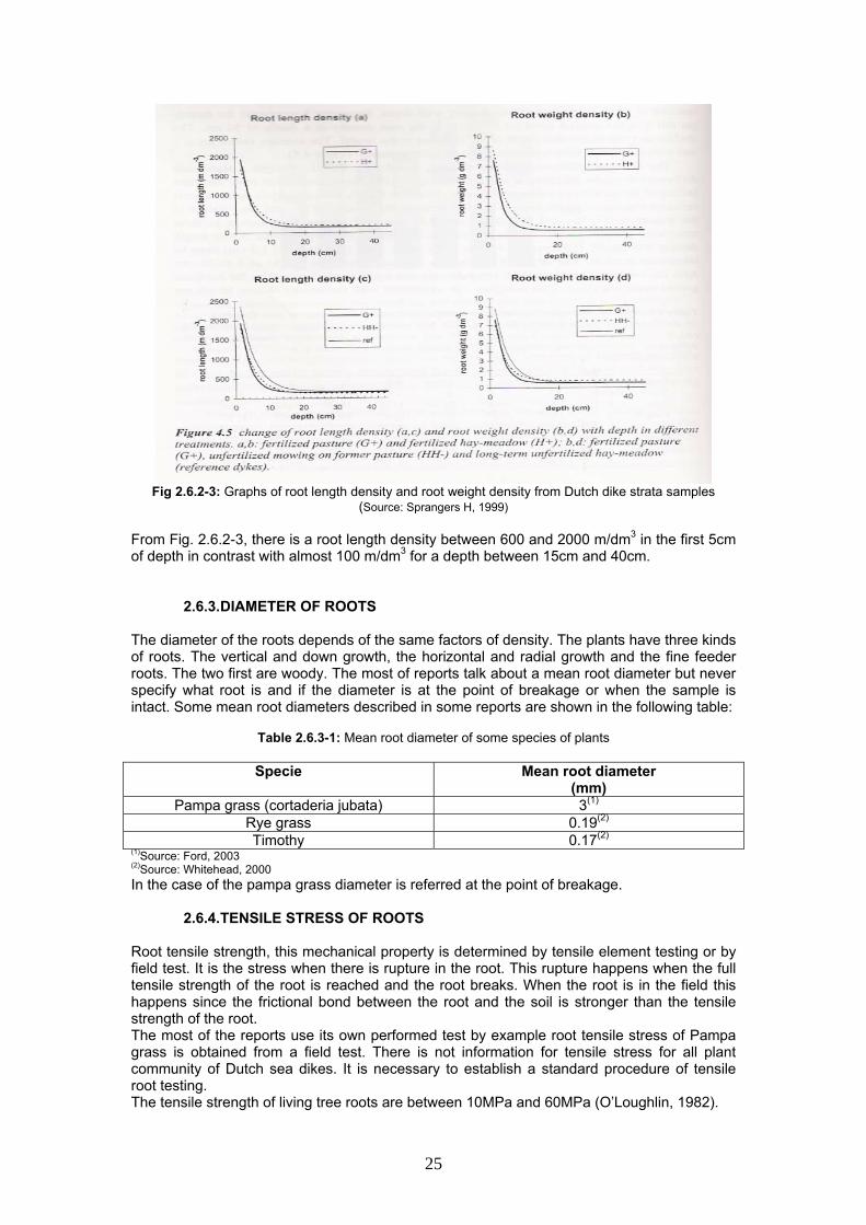
Fig 2.6.2-3: Graphs of root length density and root weight density from Dutch dike strata samples

(Source: Sprangers H, 1999) From Fig. 2.6.2-3, there is a root length density between 600 and 2000 m/dm3 in the first 5cm of depth in contrast with almost 100 m/dm3 for a depth between 15cm and 40cm.

2.6.3. DIAMETER OF ROOTS The diameter of the roots depends of the same factors of density. The plants have three kinds of roots. The vertical and down growth, the horizontal and radial growth and the fine feeder roots. The two first are woody. The most of reports talk about a mean root diameter but never specify what root is and if the diameter is at the point of breakage or when the sample is intact. Some mean root diameters described in some reports are shown in the following table:

Table 2.6.3-1: Mean root diameter of some species of plants

Specie Mean root diameter

(mm) Pampa grass (cortaderia jubata) 3(1)

Rye grass 0.19(2)

Timothy 0.17(2)

(1)Source: Ford, 2003 (2)Source: Whitehead, 2000 In the case of the pampa grass diameter is referred at the point of breakage.

2.6.4. TENSILE STRESS OF ROOTS Root tensile strength, this mechanical property is determined by tensile element testing or by field test. It is the stress when there is rupture in the root. This rupture happens when the full tensile strength of the root is reached and the root breaks. When the root is in the field this happens since the frictional bond between the root and the soil is stronger than the tensile strength of the root. The most of the reports use its own performed test by example root tensile stress of Pampa grass is obtained from a field test. There is not information for tensile stress for all plant community of Dutch sea dikes. It is necessary to establish a standard procedure of tensile root testing. The tensile strength of living tree roots are between 10MPa and 60MPa (O’Loughlin, 1982).

25

Table 2.6.4-1: Tensile stress of roots of some species of plants

Common Name Species Mean Root Diameter

rootd (mm)

Tensile stress of Roots

TR (MPa)

Pampa Grass Cortaderia jubata 3 13.7(1)

Vetiver Grass 0.73 75(2)

Couch Grass Elymus (Agropyron) 7.2 – 25.3(3)

1)Source: Ford, 2003 (2)Source: Msc Thesis of Maaskant, 2005 (3)Source: Msc Thesis of Young, 2005 Some roots like Vetiver grass have a higher tensile stress when the diameter is lower. See the Fig. next table.

Fig. 2.6.4-1: Relation between diameter and tensile stress of Vetiver roots

(Source: Msc Thesis of Maaskant, 2005) More information about tensile stress of roots for different species is described in the annex.

2.6.5. THE PULLOUT FORCE OF ROOTS It is the force in the root when there is a slipping due to bond failure. There is a slip out of the soil when the sol-root bond is broken, and the pullout force is hence a function of the surface area of the root, and the soil properties. The roots are pulled out of the soil when their frictional bonds with the soil are weaker compared with their tensile strength. It means the roots are removed from the soil due to the frictional bonds with the soil are not strong enough to allow the uptake of tension in the roots. According to Waldron and Dakessian (1981) the pullout force is calculated as (Pollen, 2005):

root

rootp d

LF

⋅⋅=

'2 τ

Where: is pullout force (KPa), 'pF τ is maximum tangential stress (KPa), is root length

(m), and is root diameter (m). rootL

rootd An example that shows the differences between the failure for break or pullout are shown in the following figure.

Fig. 2.6.5-1: Graph showing estimated pullout versus breaking forces for

River birch roots in a soil with strength of 6KPa (Source: Pollen N, Simon A, 2005)

26

2.6.6. SOIL-ROOT MATRIX COHESION

The roots provide an additional strength to the soil and this is considered like additional cohesive strength )( rootCΔ . Some investigators like 0’Loughlin (1982) says this value is between 1 and 20KPa. And others like Hähne and Tobias affirm that the gain in shear strength ranges from 5KPa to 15KPa. But both investigators do not explain at what depth of the soil.

Table 2.6.6-1: Additional cohesion in the soil due to roots according different investigators

Investigator Soil-vegetation situation rootCΔ

(based on shear tests) KPa

Swanston 1970 Mountain till soils under conifers in Alaska 3.4 - 4.4

O’Loughlin 1974 Mountain till soils under conifers in British Columbia 1.0 - 3.0

Endo and Tsuruta 1969 Cultivated loam soils (nursery) under alder 2.0 – 12.0

Waldron and Dakessian 1981 Clay loams in smallcontainers growing pine seedlings

O’Loughlin et al. 1982 Shallow stony loam hill soils under mixed evergreen forests, NZ 3.3

Source: O’Loughlin, R.Ziemer, 1982 The direct shear test is used to calculate this cohesion due to roots in the soil.

Fig. 2.6.6-1: Simple schematic of shear testing

2.6.7. ANGLE OF SHEAR DISTORTION OF ROOTS ( )θ It is the angle that the roots make with failure plane before of their breaking in the shear zone. It is assumed that the failure plane is parallel to surface of soil. Wu et al (1979) made some tests and he found that angle of shear rotation ( )θ is between

and (Pollen, 2005). 040 090

⎟⎠⎞

⎜⎝⎛=

zxarctanθ

27

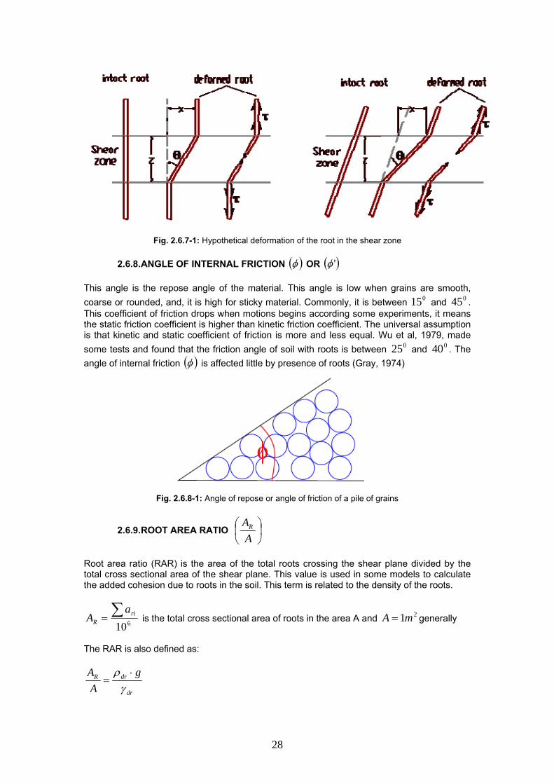
Fig. 2.6.7-1: Hypothetical deformation of the root in the shear zone

2.6.8. ANGLE OF INTERNAL FRICTION ( )φ OR ( )'φ This angle is the repose angle of the material. This angle is low when grains are smooth, coarse or rounded, and, it is high for sticky material. Commonly, it is between and . This coefficient of friction drops when motions begins according some experiments, it means the static friction coefficient is higher than kinetic friction coefficient. The universal assumption is that kinetic and static coefficient of friction is more and less equal. Wu et al, 1979, made some tests and found that the friction angle of soil with roots is between and . The angle of internal friction (

015 045

025 040)φ is affected little by presence of roots (Gray, 1974)

Fig. 2.6.8-1: Angle of repose or angle of friction of a pile of grains

2.6.9. ROOT AREA RATIO ⎟⎠⎞

⎜⎝⎛

AAR

Root area ratio (RAR) is the area of the total roots crossing the shear plane divided by the total cross sectional area of the shear plane. This value is used in some models to calculate the added cohesion due to roots in the soil. This term is related to the density of the roots.

610∑= ri

R

aA is the total cross sectional area of roots in the area A and generally 21mA =

The RAR is also defined as:

dr

drR gAA

γρ ⋅

=

28

Where: drρ is the dry root mass density (g/dm3) and drγ is the dry root unit weight (KN/dm3)

rr

dr

dr Lag

⋅=⋅⋅ 310

γρ

Where ra is the average root cross section area (mm2) and is root length density (m/dm3). This information was taken from thesis of Young 2005, with a changing in the factor of conversion. In the same thesis was found some values of root area ratio derived from information of Spranger (1999). They were calculated using

rL

300=drγ gr/dm3 and root

diameter mm. All these calculations are shown in the Fig.2.9. 13.0=d

Fig. 2.6.9-1: Graphs of root area ratio calculated from drρ and drγ of

Dutch dike strata samples tested by Sprangers (Source: Msc Thesis of Young M, 2005)

From Fig. 2.6.9-1, it is shown that the RAR is almost 0.25% for a depth between 15cm and 40cm of strata. It means almost one root of 3mm-diameter in a square of 50mm x 50mm. In depth lower than 5cm RAR is almost 3% so it is a root of 3mm-diameter in a square of 15mm x 15mm. If we make a simple visual inspection in the dutch dikes these values seems to be unreal. RAR value for Dutch dikes has to be determined by tests. This value is important for to make some calculations of soil-root matrix cohesion due to presence of roots in the following chapters.

2.7. MANAGEMENT PROCEDURE

Referring to the method to develop growth and expansion of the grass layer( sward or blades layer) as roots or turf layer, avoiding the growth of rough thicket and wooded areas. Of all of these methods the most important are haying, grazing and fertilizing. The results of many experiments on sea dikes (1991-1995) where this was applied these methods conclude the following (TAW, 1997).:

• The method of grassland management used determines the vegetation-clay composition and structure and the strength of the turf or sod against erosion.

• The turf or sod is stronger if during the process of growing grass an unfertilized hay-making and lightly fertilized grazing is carried out.

The grass cover quality of Dutch dikes has been divided into four categories according to methods used in the management of grassland for a better safety monitoring. These categories are showed in the Table 2.7-1. For a detailed information review Grass cover as a dike revetment, TAW 1999.

29

Table 2.7-1: Categories of grass cover quality according management grassland Management procedure Category Haying Grazing Fertilizing

Quality of Turf respect to erosion resistant

A 2 times/year By sheep Effective

B By sheep Lightly Reasonable/Well closed

C Intensive Poor to mediocre/open areas

D 1-4 times/year Intensive + by

horses/cattle Intensive + Herbicides Very poor

If the grass cover monitored is in the category is of poor quality, this can be improved by adjusting the methods of management which leads to a higher category. Changing the type of species compositions takes more time. In summary the researches show that there is an inter-relation between management and strength of grass cover.

FI Fig. 2.7-1: Grass growth according management grassland applied (Source: Hans Sprangers,1994)

30

3. HYDRAULIC ASPECTS Continuous swaying produces hydraulic loads on the sea dikes. In this section these hydraulic loads, which impact the sea dikes, will be described briefly. In detail we will describe the wave overtopping event, the wave overtopping design discharge and the different models which allow the calculation of these discharges. Van de Meer’s model, Schüttrumpf’s model and Besley’s model will be discussed. The flow of groundwater also produces hydraulic loads on the surface of inner slope. A wave overtopping event produces shear forces which will erode the slope.

3.1. HYDRAULIC LOADS IN SEA DIKES The surface of sea dikes are subjected to hydraulic loads generated by the wave impact, by the water running up and down and the wave overtopping. The first two hydraulic loads mentioned above(wave impact and water running up and down) occur on the outer slope. The final hydraulic load (wave overtopping) occurs on the inner slope. The wave impact compresses the impacted area and produces sideways and upward movements on the soil adjacent to impact area. The water running up and down generates uplift forces on the surface of dike. The wave overtopping causes erosion and infiltration on the surface of the crest and inner slope of the dike. See Fig. 3.1-1. In this document the loads caused by overtopping waves are crucial so they will be discussed in detail.

Fig.3.1-1: Overtopping process including main failure mechanisms (Source: http://

awww.rug.ac.be/opticrest/html/abstracttask35.pdf) According to past registers of sea dike failures, the hydraulic loads which caused more damage are the wave overtopping. This is due to the fact that these produce erosion and infiltration and thus failures in the crest and inner slope. The overtopping event is the result of waves running up on the outer slope of sea dikes to crest and it produces when (Besley, 1999):

- The wave run-up is higher to level of the see dike crest, causing the water pass over to inner slope. A continuous layer then passes over the crest and inner slope.

- The waves break on outer slope and produce significant volumes of splash. This intermittent flow is produced either by its own moment or by the force of onshore wind.

- The wind acts on the waves crests immediately offshore of the sea dikes. The water appears on the crest like a spray and need strong onshore wind to pass over it and to have a wave overtopping event.

The cover used on the inner slope of Dutch sea dikes is grass since a wave overtopping event has a low frequency of occurrence. The roots will not be permanently waterlogged, but the plants and herbs start to die. So some previous tests (CIRIA TN71) made on good grass cover show some values of maximum erosion velocities related to a duration time. These values are shown in the Table 3.1-1.

31

TABLE 3.1-1: Maximum velocities of erosion in good grass cover of inner slopes

Good Grass Cover

Maximum velocities of erosion (m/s)

Duration time (hours)

2 Prolonged period 3-4 Several hours 5 Less than 2 hours

Source: MSc Thesis of Young, 2005

3.2. WAVE OVERTOPPING DESIGN DISCHARGE Only a percentage of waves induce an overtopping event and each has its own characteristics like: overtopping discharge, layer thickness (crest and slopes) and velocity flow. To understand the crest level is important for the design of sea dikes as well as to be sure that overtopping water does not put at risk the dike and inner slope stability. Previously the calculation of crest level of sea dikes was empirical and was based on previous experience. This level was determined by adding between 0.5m and 1m to the highest observed storm and when a new event overtopped it then the crest level was increased using the same criterion. Thus the dikes were growing its height. Some Dutch sea dikes have the crest level from 4 to 5m above the design water sea level. Actually to determine the design discharge of wave overtopping several different methods exist based on the following characteristics: the return period, average overtopping rates and motion equations of water running down on clay slopes. The overtopping discharge is defined per linear meter of width. For an overtopping discharge of 1l/s per m is possible to reach maximum velocities of 4m/s – 5m/s and a layer thickness of 10cm– 40cm on the crest. The allowable overtopping, according to Dutch standards, is shown in Table 3.2-1. The value q is the average overtopping discharge in time since the instantaneous overtopping discharge is much more.

TABLE 3.2-1: Maximum overtopping discharge over inner slopes

Characteristic inner dike slope Maximum overtopping discharge

q (l/s) Any inner dike slope 0.1

Normal inner dike slope 1 High quality inner dike slope 10

Source: Van der Meer, 1993, Conceptual design of rubble mound breakwaters There are three methods to calculate the characteristic of a wave overtopping event which will be explained in the appendix. These methods are: Van de Meer, Besley and Schüttrumpf. Two of them (Van de Meer and Besley method) calculate the overtopping discharge, whereas the other (Schüttrumpf method) calculates the overtopping velocity and layer thicknesses related to the event. See appendix for more details of these methods.

32

Fig.3.2-1: Wave overtopping event at a sea dike (Source: http:// sun1.rrzn.uni-

hannover.de/fzk/e6/e6_1/icce2002_failure.pdf)

3.3. GROUNDWATER FLOW LOAD THROUGH DIKE

Flow through the dike body is not presented in dikes with waterproof dikes which is the case of Dutch seadikes, however in this item it is mentioned the load generated by this groundwater flows in the inner slope. The waves in permanent contact with the seadikes produce a flow or percolation through the dike body which can destabilize the grain located on the inner slope. This flowing is generated due to head difference across the structure. The flow through a granular medium is called porous flow. When this porous flow is flowing through the pores or voids causes a friction in the structure of the grain. This friction is the flow pressure or force which is necessary to take account when the water is coming to the surface of the inner slope since these grains can come out and consequently to produce erosion destabilizing the dike. The flow force per unit volume is defined as the following formula.

igF wf ⋅⋅= ρ or iF wf ⋅= γ

Where porous flow force, :fF :wρ water density, wγ :water specific weight, :g gravity

hydraulic gradient :ixhiδδ

=

In order for to keep equilibrium in the inner slope is necessary that the following relation between the repose angle, the inclination angle of the slope and the intersection angle of streamline with face of slope must be fulfilled.

( ) ( )( ) ( )pwws

pwws

ii

Tanθαραρρθαραρρ

φ−⋅⋅−⋅−

−⋅⋅+⋅−≥

sincoscossin

Where :sρ mass density of soil

:φ angle of repose :α angle of slope :pθ angle between horizontal and streamline at slope face

33

The before formula works for slopes of soil no cohesive whether the slope is clay or loam then the slope is steeper. The streamline can be horizontal when there is a sudden fall of the waterlevel outside a revetment or when there is a heavy rainfall on a revetment. In this case the angles are defined as it is indicated below. See Fig. 3.3-1.

0=pθ and αtan=i ⇒ αφ 2≥ if and 3/2000 mkgs =ρ 3/1000 mkgw =ρ The streamline reach to parallel to slope when there is a water flow over the dike or when there is a more permeable layer in a less permeable. The angles fulfill the relations shown below. See Fig. 3.3.

αθ =p and αsin=i ⇒ αφ TanTan ⋅≥ 2 if and 3/2000 mkgs =ρ 3/1000 mkgw =ρ

p

p

pF α−θ

α

θ

Fig.3.3-1: Force on inner slope due to porous flow How the core of sea dikes is impermeable only a flow through the revetment is present during an overtopping and this is parallel to the slope of dike. The parallel force per unit volume is represented with the following formula:

αγ SinF wf ⋅=

The thickness of the revetment is so this force per linear meter of width is expressed like: DDSinF wf ⋅⋅= αγ

3.4. HYDRAULIC BEHAVIOUR OF THE SUBMERGED GRASS The hydraulic behaviour of a channel without revetment only with the exposed soil than a channel covered by grass is different. The grass revetment produces some effects that should be considered: the hydraulic cross section reduction and the roughness elements as shape, size, arrangement and concentration. In this item based on the investigation of Carollo, 2005 is shown the used formulas to estimate the average velocity of flow which has grass revetment. The hydraulic behaviour is different for a completely submerged grass under the flow and emergent grass. When the grass is covering a channel is expected to be totally submerged but when is covering a seadikes not necessarily has to be submerged during an overtopping event since the overtopping flows could be low and it could generate a depth of water lower than 20cm that is the height of the sward, however in this item it is assumed that the grass is totally submerged.

34

The geometry of the vegetation elements and the turbulence characteristics of the flow affect the hydrodynamic resistance and the size of the vortical wakes generated downstream of the elements themselves (Shen 1973). The stubbles and the swards deflects according to the quantity of water is flowing through or over them. If the water depth is lower to length of stubbles, these are keeping in their position. When the water level is higher to length of stubbles, these deflect partially or totally on slope. When the grass is deflected totally, the shear stress are predominant but when the stubbles and swards are still stand or semi-flexed, the drag forces become important besides the depth of water is low. The grass is a flexible element and has three typical configurations when water is flowing over it. These configurations depends on flow and the bending stiffness vv IE , where is the

longitudinal modulus of elasticity of the vegetation element and

vE

vI is the moment of inertia of the cross section of the element itself. The configurations of the grass are:

- Those that do not change their position in time so they are erect. - Those that change their position in time so they are subjected to a waving motion. - Those that change permanently their position so they are prone position.

Fig.3.4-1: Geometrical features of vegetation under water ((Source: Carollo F.G., 2005)

The velocity profile of submerged flexible vegetation has a S shape (See. Fig.3.4-2).This shape is a result of measurements made by Kouwen et al (1969). It the Fig. 3.4-2 is noted two different remarkable regions, one when the element is submerged and other when is emerged. These differences increase with the vegetation concentration ( )M . The inflection point located in the top of the vegetation is noted too. In the next table there is a brief description about the velocity behaviour for different depth of water ( )h respect to the bent

vegetation height ( . )sh

Table 3.4-1: Description of the velocity profile diagram for flexible vegetation according to Carollo, 2005.

shh < Near to shh = shh > - Local velocity very low almost constant.

- Local velocity and its gradient increase. - Vertical profile u-y is concave downward. - The maxima value of turbulent shear stress and turbulent intensity. (Ikeda and Kanazawa 1996).

- The velocity gradients decrease. - Vertical profile u-y is concave upward.

35

Fig.3.4-2: Typical velocity profile of a submerged flexible vegetation. Diagram u-y in which “u” is local

velocity and “y” is the height of water from the bottom (Source: Carollo F.G., 2005)

The flow resistance law in vegetated channels was proposed firstly by Kouwen (1992). Kouwen made many test with plastic material simulating to grass. In his method is taken account the biomechanical properties of the vegetables and conclude that the vegetation is in prone configuration when the shear velocity ( )*u is higher than the critical shear velocity ( )*

cu)

.

However his method has been modified for certain quantity of concentration of stems/dm2. This method is valid for

(M50<M stems/dm2 and has the following assumptions:

- The flow resistance due to bed, in which the vegetation is rooted is negligible. - The vegetation elements are uniformly distributed on the bed - The flow regime is fully turbulent.

⎟⎟⎠

⎞⎜⎜⎝

⎛⋅+=

shhCC

uV log10*

Where (m/s) is mean flow velocity, (m/s) is shear velocity and , are numerical coefficient (See Table 3.4-2).

V *u 0C 1C

Thes shear velocity is calculated like ghIu =* For to estimate the bent vegetation height ( )sh is used the following relation (Kouwen and Li

1980). It depends of the concentration ( )M , the vegetation height in the absence of flow

and bending stiffness( vH ) ( )vv IE .

463.0

4.3⎥⎥⎦

⎤

⎢⎢⎣

⎡⎟⎟⎠

⎞⎜⎜⎝

⎛⋅⋅⋅⋅⋅=

v

svwvv H

hHIhIME γ

The critical shear velocity is calculated with the next expressions. The first is used by low values of aggregate stiffness since the elements return to the non-deformed configuration when the flow finishes. The second is for high values of vv IME when the stems remain in a bent configuration. In general use the minimum critical shear velocity between two expressions.

2* )(33.6028.0 vvc IMEu += 106.0* )(023.0 vvc IMEu =

36

The numerical coefficient of Kouwen has been modify since the investigation made by Carollo

et al, 2005, found that the hypothesis of the *uV

decreases for increasing values of the

concentration is not always true.

Table 3.4-2: Recalibrated Coefficient of Kouwen’s flow resistance law

Recalibrated Kouwen’s method *

*

cuu range

0C 1C

Erect 1*

*

≤cu

u 1.91 11.5

Prone 5.11 *

*

≤<cu

u 4.63 22.4

Prone 5.25.1 *

*

≤<cu

u 0.93 22.4

Prone 5.2*

*

>cu

u -1.81 22.4

Source: Carollo F.G., 2005. The original coefficients have been recalibrated by investigation of Carollo et al,2005. For estimating high values of M was developed a new relation of flow resistance by Carollo et al, 2005. The following assumptions were made during the elaboration of this formula:

- Rigid and straight prismatic channel. - Flow without sediment transport - Vegetated elements are uniformly distributed - Underestimation of vegetation rooted when the dissipative effects are analyzed. - Application of Π-theorem (Barenblatt, 1979)

The new flow resistance law is:

( )321 *

0*

a

s

v

a

w

s

a

s hHhu

hhMA

uV

⎟⎟⎠

⎞⎜⎜⎝

⎛⋅⎟⎟

⎠

⎞⎜⎜⎝

⎛⋅⎟⎟

⎠

⎞⎜⎜⎝

⎛⋅=

ν

The coefficients ( )( 321 ,,, aaaMAo ) are shown in the Table 3.4-3 for different concentration of stem per square decimeter.

Table 3.4-3: Coefficient of Carollo et al’s flow resistance law

M

stem/dm2 ( )MA0 1a 2a 3a

≤ 50 0521.14.43 −M 1.168 0 -0.861 ≥ 280 3701.20275.0 M 1.168 -1.023 -0.861

Source: Carollo F.G., 2005.

M has to be considered equal to the ratio oM

Min which is reference concentration set

equal to 1 stem/dm2. There is not information for concentration between the range of 50-280 stem/dm2.

oM

37

3.5. OVERTOPPING FLOW LOADS The water running down to slope develops hydraulic forces during an event of overtopping. Theses forces are acting directly to each soil particle of the revetment. The particle movement of a non-cohesive soil will occur if the instantaneous fluid force on a particle is larger than instantaneous resisting force related to the submerged particle weight and the friction coefficient . If the soil is composed by clay or silt particles the cohesive forces need to be considered. The soil particles involved by roots and geosynthetics has an extra cohesive resisting forces that are important when the detachment of this particles is analized. The forces acting on a sediment particle resting on the bed of a channel are depicted in the sketch below.

clay-root-geosynthetics

CohesionF

FDSF

W FFA

FLLF

A FF

W

FSDF

Fig.3.5-1: Shear Forces acting on a loose grain and on reinforced grass revetments

3.5.1. SHEAR STRESS OF WATER

The knowledge about the behaviour of soil which is located in the matrix root-soil of grass exposed to current is scarce so the same classical definitions of shear water force are going to be explained in this item. The different velocities on adjacent streamline or in better way vertical changes in water velocity are the cause of the shear water force. There is a difference in velocities and in pressures above and below grains at the water-slope interface so the velocity of water generates shear forces on the revetment of slope. These shear forces acting on the bed of the slope generate shear stress, which initiate bedload movement. The theories say that the shear force acting on a grain no-cohesive is proportional to square flow velocity and the surface exposes to flow either a uniform flow or a turbulent flow. So the shear water force is: (See Fig. 3.5-1) SwfS AucF ⋅⋅⋅= 2ρThis shear water force applied to a plane surface per unit area can be expressed by shear

stress like ( )2*uw ⋅= ρτ . is the local near bed-velocity and proportional to . The term

is named shear velocity or friction velocity.

u *u*u

For uniform flow conditions the movement of particles is calculated by the Shields diagram using the concept of a mobility parameter which in function of shape of particle, velocity profile, critical shear stress. His tests demonstrated that the flow condition near the bed is in function of the ratio of grain size and the thickness of viscous sub-layer. He introduces the parameter called Reynolds number that is based on grain size and shear velocity. An

empirical relation between the parameters ( ) dgws

c

⋅⋅− ρρτ

and υ

duc ⋅*

was introduced by

shields. He correlated the rate of sediment transport with τ and defined cτ by extrapolating to zero material transport. He uses the same relation of Breusers (1986) but for critical state.

38

This relation is:

( )( ) ( ) ( )

⎟⎟⎠

⎞⎜⎜⎝

⎛ ⋅==

⋅⋅Δ=

⋅⋅−==

υρρτ

ψdu

ffdg

udgstrength

load cc

ws

cc

*

*

2*

Re

Where: w

ws

ρρρ −

=Δ and if 1<ψ the particle is motionless

Although the critical shear stress is defined by Shields for different loose grains and it is applied not only to single particles but also a flat bed with relatively small grain, it is complicated to apply this concept on the particles located in the matrix root-soil of grass since they have additional cohesion forces produces by the root. The vortex in the flow which is flowing through stubbles and swards generates turbulence so the conditions of flow changes. If we refer about the reinforced grass revetments (grass with geocells or geogrids), there are additional cohesion forces acting on soil particles which are inside of cell. Shear stress:

In the open channel, Shear stress can be defined as the force of moving water against the bed of channel. The shear stress of a steady uniform flow is a function of water surface slope, channel geometry and flow. It is calculated as:

hIgwb ⋅⋅⋅= ρτ or hIwb ⋅⋅= γτ for small slopes of the bed (and water

surface and energy line) I Shear stress in beds with flexible submerged vegetation: The grass stems dissipate shear force before it reaches soil surface and stabilize the soil surface against turbulence fluctuations so only a part o this shear stress reaches to impact the soil. For to calculate this effective shear stress ( )eτ acting on the soil located under the vegetative revetment, the U.S. Deparment of transportation (September of 2005) has development a equation where variables like grass cover, soil grain roughness, manning’s roughness coefficient for grass linings have been considered. In this item all these procedures is shown and details of some coefficients are in the annex. The flow depth and shear stress increase when the grass stems bend. The prone position of the stems reduces the roughness height and increase velocity and flow rate. The shear stress is moved away form the soil surface due to stems only a portion of this shear produce impact on the soil. The next equation developed by USDA, 1987 allow to calculate the effective shear stress ( )eτ .

( )2

1 ⎟⎠⎞

⎜⎝⎛⋅−⋅=

nn

C sfde ττ

Where ( )( )2/ mNdτ

sn is the design shear stress , is the grass cover factor (these values

are in the annex), is the soil grain roughness (See Table 3.6 ) and is overall lining

roughness. The design shear stress

fCn

( )dτ is chosen a criterion however it could be replaced by the stress in the bottom of the channel to estimate how much effective shear stress is acting on the soil directly. In this method when is mention that the part of the shear stress reaches the soil is not mentioned what shear stress is at the top or at the bottom of the grass.

39

Table 3.5.1-1: Values of soil roughness in function of 75D

75D sn < 1.3mm 0.016

> 1.3mm ( ) 61

75015.0 D⋅ Source: U. S. Department of transportation (2005).

The overall lining roughness is in function of grass roughness coefficient

(whose values are in the annex) and mean boundary shear stress

4.0−⋅= bnCn τ ( )nC( )( ) I⋅hmN wb ⋅= γτ 2/

The soil under the grass cover can not be eroded if the effective shear stress ( )eτ is lower

than the permissible soil shear stress ( )soilp,τ ( soilpe ,ττ ≤ ). The U.S. Department of

transportation (September of 2005) establishes soil,pτ for non-cohesive soils and cohesive soils, the equation used is shown in the Table 3.7

Table 3.5.1-2: The permissible soil shear stress ( )soilp,τ according to U. S. Department of

transportation

Type of soil The permissible soil shear stress (N/m2)

mmD 3.175 < 1, =soilpτ Non-cohesive

mmDmm 503.1 75 << 75, 75.0 Dsoilp ⋅=τ

Cohesive 62

54322

1, )()( cecccPIcPIcsoilp ⋅⋅+⋅+⋅+⋅=τ

In the case of cohesive soils PI is the plasticity index, is void ratio and coefficients

which depends on type of soil and plasticity index are explain in detail in the annex.

e654321 ,,,,, cccccc

If we made soilpe ,ττ = , the permissible shear stress on the vegetative lining ( )vp,τ can be

calculated making vp ,d ττ = so the next expression can be used:

2,

, )1( ⎟⎟⎠

⎞⎜⎜⎝

⎛−

=sf

soilpvp n

nC

ττ

3.5.2. DRAG WATER FORCE The drag water force ( D is the force that resists the movement of a particle soil or tails through water so it is the resultant of all friction forces. This force is the effect of the viscous friction and the pressure force so as shear force is proportional to square velocity and it has the following expression:

)F

DwDD AuCF ⋅⋅⋅= 2ρ or ( )22

41

21 duCF wDD ⋅⋅⋅⋅⋅⋅= πρ

Where flow velocity at particle centre is u , particle diameter is and the drag coefficient is

. This drag coefficient is in function of the local Reynolds number

d

DC ⎟⎠⎞

⎜⎝⎛ ⋅

νdu* .

40

The flow velocity at particle centre has the following expression *2 uu ⋅= α . This 2α -coefficient are in function of the local Reynolds number if the regime is hydraulically smooth and in function of bed shear velocity. The drag force can be expressed as:

2*

23 udF wD ⋅⋅⋅= ρα where the coefficient is

823DC

⋅= παα and depends of the local

Reynolds number. In the calculation of shear stress (Shield), these forces were neglected in the evaluation of particles equilibrium since small particles has low exposed area to perpendicular flow. Nevertheless, on a grass revetment, drag forces become to be important when the water depth is low and the sward and stubbles are stand or semi-deflect. The same comment we could say for reinforced grass revetments since the geocells and the geowebs do not have exposed area on the outer layer.

3.5.3. LIFT FORCE Lift force is in the direction normal to the flow. This force tries to remove vertically the particle of soil. It is related to the velocity squared, thus if the velocity increases a little bit, lift force could have large changes. In flows with turbulent conditions the lift force is fluctuating and it is important for particle stability. It is defined like:

max2

41 pdFL ⋅⋅⋅= π

Where: is the difference between the positive and negative pressure peaks,

maxp

p oτ⋅=18max (Emmerling 1973). The new expression replacing this value is:

ooL ddF τπτπ ⋅⋅⋅=⋅⋅⋅⋅= 224

1 5.418

At the same time but 2*uwo ⋅= ρτ

o

oo

cUr

u⋅

=* for a turbulent flow according

Rijkswaterstaat (Hoffmans, 2006). The lift forces could be expressed in function of the depth-averaged relative turbulence intensity ( )or , the average-velocity or V and coefficient

. Thus the next expression defines the lift force: oU

2.1=oc

⋅⋅⋅⋅⋅⋅= 222

25.4 Vrc

dF oo

wL

ρπ

The shear stress oτ acting on the particle is a portion of the shear stress when is covered by grass so if we use the shear stress effective proposed by U.S. Department of transportation (September of 2005) the new expression of the lift force would take account the quatity, quality and phisci characteristics of the grass and it could be defined like:

( )2

2 15.4 ⎟⎠⎞

⎜⎝⎛⋅−⋅⋅⋅⋅=

nn

CdF sfoL τπ

41

This expression could be modified using the shear stress defined by Hoffmans, 2005 2

⎟⎟⎠

⎞⎜⎜⎝

⎛ ⋅⋅=

o

owo c

Vrρτ thus the lift force is:

( )2

222

2 15.4 ⎟⎠⎞

⎜⎝⎛⋅−⋅⋅⋅⋅⋅⋅=

nn

CVrc

dF sfo

o

wL

ρπ

Where the grass cover factor ( )fC , soil grain roughness ( )sn , overall lining roughness are defined by U.S. Department of transportation (September of 2005). See annex.

( )n

However, according to late investigations made by Carollo, 2005 the averaged-velocity ( )

can be expressed in function of concentration

V( )M , depth of water ( )h , bent vegetation

height ( , slope and the vegetation height in the absence of flow )sh ( )I ( )vH . Thus the lift force for a turbulent flow with the presence of grass can be expressed as:

( )321 222

222

25.4a

s

v

a

w

sa

soo

o

wL h

HhghIhhMAghIr

cdF ⎟⎟

⎠

⎞⎜⎜⎝

⎛⋅⎟

⎟⎠

⎞⎜⎜⎝

⎛ ⋅⋅⎟⎟

⎠

⎞⎜⎜⎝

⎛⋅⋅⋅⋅⋅⋅⋅=

νρ

π

Where for hydraulically smooth conditions 05.0=or and for hydraulically rough conditions

, and the coefficient (Hoffmans, 2005). 15.0=or 2.1=oc The new expression of lift force for smooth condition, where the roughness elements are submerged to laminar layer that is they do not have influence in the friction of the flow, can be expressed like:

( )321 222

22025.0a

s

v

a

w

sa

sowL h

HhghIhhMAhIdF ⎟⎟

⎠

⎞⎜⎜⎝

⎛⋅⎟

⎟⎠

⎞⎜⎜⎝

⎛ ⋅⋅⎟⎟

⎠

⎞⎜⎜⎝

⎛⋅⋅⋅⋅=

νγ

The new expression of lift force for rough condition, where the roughness elements are protruding into far the turbulent flow and dominate the flow resistance, can be expressed like:

( )321 222

22221.0a

s

v

a

w

sa

sowL h

HhghIhhMAhIdF ⎟⎟

⎠

⎞⎜⎜⎝

⎛⋅⎟

⎟⎠

⎞⎜⎜⎝

⎛ ⋅⋅⎟⎟

⎠

⎞⎜⎜⎝

⎛⋅⋅⋅⋅=

νγ

In summary, replacing the different Carollo’s coefficient ( )oA for different concentration ,

the lift force could be represented in the ways shown in the Table 3.5.3-1.

( )M( LF )

42

Table 3.5.3-1: The lift force values replacing values of Carollo et al, Hoffmans ( LF )and U.S. Department Transportation

Conditions Lift Force (N)

M≤5

0 st

em/d

m2

722.1336.2105.222.46

−

−⎟⎟⎠

⎞⎜⎜⎝

⎛⋅⎟⎟

⎠

⎞⎜⎜⎝

⎛⋅⋅⋅⋅=

s

v

swL h

HhhMhIdF γ

Sm

ooth

con

ditio

ns

r o=0

.05

M≥2

80

stem

/dm

2

722.1046.2336.274.4251086.1

−−

−⎟⎟⎠

⎞⎜⎜⎝

⎛⋅⎟

⎟⎠

⎞⎜⎜⎝

⎛ ⋅⋅⎟⎟

⎠

⎞⎜⎜⎝

⎛⋅⋅⋅⋅⋅=

s

v

w

s

swL h

HhghIhhMhIdF

νγ

M≤5

0 st

em/d

m2 722.1336.2

105.221.416−

−⎟⎟⎠

⎞⎜⎜⎝

⎛⋅⎟⎟

⎠

⎞⎜⎜⎝

⎛⋅⋅⋅⋅=

s

v

swL h

HhhMhIdF γ

Rou

gh c

ondi

tions

r o=0

.15

M≥2

80

stem

/dm

2

722.1046.2336.274.4251071.16

−−

−⎟⎟⎠

⎞⎜⎜⎝

⎛⋅⎟

⎟⎠

⎞⎜⎜⎝

⎛ ⋅⋅⎟⎟

⎠

⎞⎜⎜⎝

⎛⋅⋅⋅⋅⋅=

s

v

w

s

swL h

HhghIhhMhIdF

νγ

The most general equation of the lift force is:

( )321 222

222817.9a

s

v

a

w

sa

sowoL h

HhghIhhMAhIdrF ⎟⎟

⎠

⎞⎜⎜⎝

⎛⋅⎟

⎟⎠

⎞⎜⎜⎝

⎛ ⋅⋅⎟⎟

⎠

⎞⎜⎜⎝

⎛⋅⋅⋅⋅⋅=

νγ

3.5.4. COHESIVE FORCES These forces are important when the bed of the overtopping flow consists of: silty and muddy materials. But this cohesive forces not only depends the type of material, the presence of roots and geosynthetics produces also an additional cohesion in the soil. Respect to the material, the cohesion effect could be more or less pronounced depending of the type of clay mineral. Flume experiments realized by Van Rijn demonstrated that an amount of 25% of clay in a sand bed caused a significant reduction (factor 30) of the sand concentrations generated by wave action. Information about how the roots and geosynthetics help in the reduction of movement possibility of soil is scarce. The erodibility of cohesive soil is governed by the rate of consolidation. The erosion resistance increases with the compaction of the soil by example the old compact clay soils are highly resistant against erosion. Silty or clayey sand bed shows a remarkably increased resistance against erosion. Some test made by Delft Hydraulics (1989) on bed samples from the North Seas with particle sizes

between ( 50D ) mμ200100 − and mud-silt percentages between %202 − measured the critical bed shear stress related to the critical bed-shear stress according to Shields and yielded:

( ) shieldscscr P ,5.0 ττ ⋅=

Where: is the percentage of fines (mud, silt) smaller than sP mμ50 (in % minimum value equal 1%)

43

4. GEOTECHNICAL ASPECTS

4.1. CLAY AND SAND AMONG TURF The soil located among the roots of turf in the inner slope of dutch dikes is basically clay with a percentage of sand. The top layer has a thickness of 0.30m in average and it is a more sandy material since benefit plant growths. Even though the sand has low nutrients benefits the best-rooted turf or sod and so the erosion resistance is better. The microorganisms and organic material interconnect with these particles and modify their natural properties. It is recommended in the top layer a content of sand no higher than 50% (TAW, 1997) even though other studies suggest until 70% (Van den Bos, 2006). It must be remarked that for both cases the classification of soil changes since the soils are sandy when the content of sand is more than 70% and clayey when the content of clay is more than 40%. In the Table 4.1.1, it is shown how the classification of this top layer can change when the maximum recommended quantity of sand is changed therefore if the maximum sand recommended is 50% like TAW then the soil is clayey sand and if it is 70% like Van de Bos the classification of soil can be modified to sandy clay. The top layer is laid down on a layer with higher content of clay previously applied for to manage the residual strengths or for to process the local clay. The underneath layer has a higher percentage of clay. The crest and inner slope of Dutch sea dikes has a layer of clay between 1.00 to 1.50m thick. Regarding to content of sand it is recommended to make some test with sand between 50% and 70% to describe in detail the behaviour of the root-soil matrix respect to verify the behaviour of the roots in this new situation.

Table 4.1-1: Classification of soil into the turf if it has the maximum recommended quantity of sand

Classification of soil according to content of sand and clay.

Percentage content of Sand recommended in top of the

layer

Percentage content of Clay

Clayey sand 50% 50% Sandy clay 70% 30%

Fig. 4.1-1: Some differences between clay soil and sandy soil

44

4.1.1. THE MECHANICAL BEHAVIOUR OF SOIL UNDER STRESSES The soil like other material shows specific deformation behaviour before to reach the state of failure. The forces which are acting on between each particle of soil are in equilibrium so the resulting forces at any plane of soil must be in equilibrium too. Considering the area A of soil of the plane of resulting forces, the stresses can be discomposed in a normal stress

perpendicular to contact area and a shear stress parallel to contact area.

'nσ

'τ

Fig. 4.1.1-1: Forces acting on the particle of soil

The mechanical behaviour of soil under normal stress is described by Hooke’s law. It means the modulus of elasticity ( is the slope of the stress-strain curve for elastic material and in the case of soil that is non-elastic material is the tangent of secant value at a certain stress level. Thus:

)E

εσ

ddE '

=

The normal effective stress causes an elastic compression of the grain and the deformation is small. The mechanical behaviour of soil under shear stress is defined like the lateral displacement in the upper face relative to lower face of soil. The shear strain is represented by the angle γ

since γγ =Tan . The modulus of rigidity or shear modulus ( )G is the slope of shear stress-shear curve. The mutual shear deformation of individual grains causes a higher deformation than normal effective stress but this deformation is indicated a rearrangement or shearing. When the shear stress becomes larger than the product of friction coefficient and normal stress the rearrangement occurs. This rearrangement could be a compaction or a dilation of a grain mass.

Fig. 4.1.1-2: Shear stress in soil

45

The phenomenon of compaction happens when the maximum friction is reached after small shifts in the soil. The water molecules located around each clay platelet is dissipated during former overburden pressures. The phenomenon of dilation happens when after a relatively small deformation and decreasing of volume due to rearrangement of soil particles the deformation continues since in a very dense configuration the particles start climbing on top of each other brings about the increasing of volume.

Fig. 4.1.1-3: Phenomenon of dilatation and compaction in sand soil

4.1.2. SHEAR STRESS OF SANDY CLAY The top layer of sandy clay soil can be described by the tendency of the particles to stick together, this property is called cohesion, and by its natural tendency to resist movement, this is the friction angle. The presence of roots and geosynthetics give them an additional cohesion which will be revised in the next items. These properties define the frictional resistance of soil. This varies with the normal stress applied on the shear plane and it is assumed that cohesion resistant is constant and independent of applied stress (Coulomb’s law of soil shear strength). The soil is always exposed to moist conditions and even more during the wave overtopping is saturated depending on event time, it could be said that under this conditions the strength which control the volume change is the effective strength so the real shear stress on the failure plane for a drained soil is:

'''' cTanff +⋅= φστ In order to evaluate cohesion and friction angle is necessary to be similar to drained since it has a percentage of sand and unconsolidated as on the surface. This assumption is also valid for the soil located between geocells or geogrids. The moisture is the major cause of landslides due to water changes the characteristics of soil among the turf. Once this soil becomes saturated the weight of the mass of soil increases so the mass slumps and the sticky property reduces so cohesion of clay decreases almost to zero in this moment only cohesion produced by roots are working.

46

Table 4.1.2-1: Characteristics of different soils

Type of soil

Friction angle of

soil 'φ

(degrees)

The effective cohesion

'c (Kpa)

Dry unit weight

dγ (Kpa)

Saturated unit

weight

satγ (Kpa)

Elastic Modulus

soilE (Mpa)

Poisson ratio

Sandy Clay(1) 26o-28o

Fat clay slightly plastic(2) 15.1-18.1 17.3-21.3

Non-cemental clays(3) 5-10 Silty sand(4) 10-17 0.20-0.40

Medium dense sand(4) 17-28 0.25-0.40 Sand slightly silty clayey 270-32.50 --- 18-19 20-21 25-35 Sand greatly silty clayey 250-300 --- 18-19 20-21 20-30 Clay slightly Sandy weak 22.50 0 --- 15 1.5 Clay sligthly Sandy moderate 22.50 10 --- 18 3 Clay sligthly Sandy solid 22.50-27.50 25-30 --- 20-21 5-10

Clay greatly Sandy 27.50-32.50 0-2 --- 18-20 2-5 Clay organicweak 150 0-2 --- 13 0.5

Clay organic moderate 150 0-2 --- 15-16 1-2 Source(1): Una guia para la instalacion de muros modulares de allan block, 2006, allan block corporation Source(2) :Soil Mechanics, J. Brinkman, 2005, p:ST21 Source(3) :The civil engineering handbook, W. F. Chen, 2000, p:710. Non-cemented clays with pre-consolidation stress of less than 500 to 1000 kPa. Source(4) :The civil engineering handbook, W. F. Chen, 2000, p:713 Source(5) :Manual for Structural Hydraulic Engineering, S. van Baars, H.K.T.Kuijper, p:26-9

4.1.3. RESIDUAL SHEAR STRESS Residual shear stress refers to remain shear stress of a failure plane that has slipped before. Essays development by Skempton (1964) proved that the shear strength on clay slope through of a failure plane is lower than shear strength of the same plane without previous slip. The residual strength is lower than peak strength; this is caused due to formation of very thin layer of fine clay particles orientated and parallel to each other in the shear direction of slipped failure plane. Initially these particles would have a random orientation this means it was needed a higher shear strength (peak) to produce slips. The presence of sand in the layers of sandy clay increases the residual strength due to its spherical shape and roughness which can not oriented in the shear direction of failure plane like clay particles. This shear increases with increasing percentage of sand in the soil. The residual friction angle ( 'rφ )

decreases if the percentage of clay increases (Smith, 1982). The residual friction angle ( 'rφ ) for clay minerals (kaonlinite, illite and montmorillonite) range from 40 – 120. For clays that are deformed slowly to large strains under drained conditions is recommended to use residual friction angle ( 'rφ ). Respect to sand soils when this is loose, the residual strength is the peak strength but when this is dense, it is lower. The presence of cracks shows possible failure planes and the shear strengths at the plane of the contact is probably the residual shear strength. For consolidated clay the cohesion and effective cohesion is zero since it behaves like loose sand (Lambe and Whitman, 1979). According to some investigations (Crabb and Atkinson, 1991) the values of effective strength are low in superficial depth of clay soils so the Coulomb-Mohr model can be replaced for the following model:

bnp A '' στ ⋅= Where A and b are empirical soil parameter and according test of Crabb and

Atkinson, 1991 the values of A is 1.85 - 3.71 and b is 0.58 – 0.76 for shallow slip failures, where ( )2/ m' kNpτ is peak shear strength and ( )2/' mkNnσ normal effective stress and

( ) αγγσ CosDwsat ⋅⋅−=' submerged weight of the soil.

47

The presence of an area of cracks shows possible failure plane so the shear strengths present are residuals and depends of softening degree of clay structure and the residual angle. They are expressed like: rnr Tan ''' ϕστ ⋅= The shear stress at the contact plane between soil and geosynthetic depends of friction angle of interaction between these surfaces. If we expect that this contact surface is failure plane so it is reasonable to apply the basic concept of residual shear where after the failure event when the soil is clay or dense sand. The shear force at the contact is defined as the frictional force which is in function of the weight of soil over the geosynthetic and the friction angle of soil-geosynthetic interaction ( )gs /δ .

( )gssgs TanD // δγτ ⋅⋅= or ( ) ( )gswsatgs TanD //' δγγτ ⋅⋅−=

δτ

γ

Fig. 4.1.3-1: Frictional force in the contact plane between geosynthetic and soil of a reinforced revetment

4.1.4. SHALLOW SURFACE SLIP

It is a failure parallel to the surface of soil. This kind of failure is more present in grass revetments and when the water is flowing soil starts rolling up. This shallow surface slip is typical of homogeneous cohesionless soil where the failure is close to the superficies of slope. For homogeneous cohesion soil is either a typical deep-seated circle or a toe circle (Mc. Carthy, 1998). It could be applied a simple equilibrium force to calculate the stability of revetments for this case of failure so this criterion will be used to analyze the stability in a reinforced grass revetment. By example, a sample of reinforced revetment is analyzed under the assumption that plane failure is at the contact surface between soil and geosynthetic so analysis of equilibrium forces acting on the sample should be applied. The forces parallel to slope should be in equilibrium so weight component parallel to slope should be equilibrated by the shear forces produces in the contact between geosynthetic and soil-root thus:

∑=⋅i

FCosWs τα where is the weight of soil and sW ∑ iFτ is the sum of shear forces

as friction force between soil and geosynthetic, shear force of cohesion and shear force of root cohesion.

γ

Σ τ

γ αα

α

γD

Fig. 4.1.4-1: Equilibrium forces parallels to slope at reinforced grass revetment

48

4.2. SHEAR STRESS IN THE SOIL-ROOT MATRIX The roots are fibers relatively strong to tensile strengths. They get stronger the low tensile and shear strengths of the soil when they are interlinked to each other. Field tests show that the finer roots with 1mm to 20mm of diameter are the most contribute to reinforce the soil than the larger. Some methods that help to quantify the shear stress effects of the root in the soil are:

• Shear tests of matrix soil-root in situ. • Formulae that allow to establish the relationship between root and soil and to

estimate the additional cohesion that generates roots in soil. These calculations can be made using some models: the simple perpendicular root model of Wu et al (1979) and fiber bundle model in roots or called also riproot of Pollen and Simon (2005).

4.2.1. THE SIMPLE PERPENDICULAR ROOT MODEL This model allows calculating the additional cohesion given by roots to soil. It is based on the Mohr-Coulomb equation '''' cTanff +⋅= φστ where the shear stress is represented by the sum of cohesion and frictional forces. The simple perpendicular root model assumes that the position of root respect to surface soil or failure plane is perpendicular. The tensional stress is acting on the root distorts it thus

the root forms a shear distortion angle

( )rT( )θ with the perpendicular axis to surface. The

tensional stress of root could be discomposed in parallel ( )rτ and perpendicular ( )rσ

stresses to surface and in function of tensile stress for a root-i ( )riT . (See Fig.4.2.1-1).

Fig. 4.2.1-1: Root crossing the soil shear zone and stressed in tension

The parallel stress is defined as θτ sin⋅= Rr T and the perpendicular stress is

θσ cos⋅= Rr T for a root with average tensile stress equal to . These values are replaced in the Mohr-Coulomb equation to estimate the additional cohesion and friction in the soil due to presence of roots.

RT

The initial models assumed that the presence of the roots in the soil only produce an increment in the shear strength ( )rτ and it is represented like an increment in the cohesion of soil-root matrix. However subsequent models like of Wu et al (1979) and Luckman et al (1982) consider that not only the cohesion but also the friction in the soils is incremented by the presence of the roots so they introduced the simple perpendicular root model. The additional cohesion produced by all roots in this model (Wu et al, 1979) is defined as:

[ ]θφθ sin'tancos +⋅⋅⋅=Δ srR

Rroot AATC

49

Where is average tensile stress of roots per unit area of soil shear zone (kPa), is the total area of roots,

rt RAA is the area of shear stress and θ is distortion angle.

The average tensile stress of roots is defined asii

iii

rr

rrrR an

anTT

⋅Σ

⋅⋅= ∑ where is the

tensile strength of roots in size class i, is section area of root in size class i and is

number of roots in size class i. The total area of roots is defined as . The

distortion angle is

irT

⋅ir

air

air

n

∑= irR nA

⎟⎠⎞

⎜⎝⎛=

zxarctanθ where x is the horizontal distortion of the root and is

the depth of the shear stress zone where the root is deformed.

z

The factor [ ]θφθ sin'tancos +⋅ sr is almost insensitive to changes of distortion angle ( )θ .

For large deformations ofθ , the factor can reach a value of 1.2 (O’Loughlin 1982) so the cohesion can be expressed like:

AATC R

Rroot ⋅⋅=Δ 2.1

The models mentioned above are defined for roots of trees and in summarize according to the simple perpendicular model the additional strength in the soil depends the amount of roots

present and the tensile strength of those roots. The quotient AAR is known as root area ratio

and it is represented with the abbreviation RAR. The next graph shows the additional cohesion for a root of 3mm of diameter for different tensile stress and root area ratio. The RAR calculated for Dutch dikes is 0.25% (Msc Thesis of Young M, 2005). Applying the equation of O’Loughlin, the additional cohesion is almost 5KPa for roots that can resist 10N or 1kg of tensile force and have this RAR. A tensile of 10N or 1 kg is reasonable value for common grass roots. For a RAR higher than 1.5%, the root cohesion is higher than 25Kpa but some tests made about root cohesion affirms that it is between 1-20Kpa (0’Loughlin, 1982) thus for value of RAR equal to 3% ( for depth lower than 5cm according to Young, 2005) the root cohesion is out of this range. And visually it is noted the grass revetment in dikes has more than 3% or its equivalent a root of 3mm-diameter in a square of 15mm x 15mm.

Root Cohesion for diferent Root area ratio (formula: Wu et al,1979; O'Loughlin 1982)

(Diameter=3mm)

0

5

10

15

20

25

0.0% 0.5% 1.0% 1.5% 2.0% 2.5% 3.0%Root area ratio "RAR: Ar/A"

(%)

TR=0.7Mpa

TR=1.4Mpa

TR=2.8Mpa

TR=4.2Mpa

TR=5.7Mpa

Roo

t Coh

esio

n

"∆C"(

Kpa

)

Ft=5N

Ft=10N

Ft=20N

Ft=30NFt=40N

Fig. 4.2.1-2: Root Cohesion for a 3mm-diameter root with different RAR and Tension Stress

50

From this draft calculation is recommendable to have real values of RAR for grass revetments of Dutch dikes as well as factor [ ]θφθ sin'tancos +⋅ sr . The tension stress should be defined since the model depends of the tension stress and this tension appears when a force is directly applied to the root thus if there is not force acting on the root there is not cohesion in the soil and it noted that affirmation is false.

Some disadvantages mentioned by other investigator are:

• The roots are not perpendicular to slip plane. The angles of the roots respect to forces acting on the soil are important since this dictates the distribution of stresses within the root so the maximum tensile strength depends of this situation.

• The roots are not mobilized when the soil shears but at much larger displacements. • The roots can be pulled out when they are tensioned. There are two mechanism of

failure in the roots: pullout (when the bond failure) and rupture (tension failure) Making a model of how the root increases the cohesion in the granular soils is more related to volume of pore since they are reduced when the roots are present. The cohesion root could be expressed like a functional expression”

( )RLDAdVVVVfc rawsp ,,,,,, 50=Δ

Where is pore volume, is soil volume, is water volume, is air volume, Soil

size where 50% of the material is finer,

pV sV wV aV 50d

rA is the average root area and RLD is root length density.

4.2.2. THE FIBER BUNDLE MODEL IN ROOT Pollen and Simon (2005) based on the concept that not all the roots are mobilized instantaneously at the moment of slope failure so they develop other method. This is based on the mode of progressive failure and it is described by fiber bundle model in material science. The roots have different tensile strengths and thus they break progressively, the load that they receive is redistributed again when some roots fail. Some test have demonstrated that the perpendicular root model overestimate root reinforcement by up to 50% in situation where slopes driving forces so great and enough to break all the roots.

4.3. BEHAVIOR OF REINFORCED SOILS UNDER STRESSES The geo-synthetics have better soil strength because they generate higher confinement among soil granules. Due to this confinement, the soils with geo-synthetics have a higher resistance to horizontal forces and lower horizontal deformations.

4.3.1. REINFORCED SOIL UNDER VERTICAL STRESSES The reinforced soil techniques are based on the principle described by Jewell in 1980 who describes that when a vertical stress vσ over a soil element as part of an infinite mass of soil is applied, two important effects are produced in the internal configuration of the soil. First the horizontal deformation in the element and second the apparition of horizontal stress

hσ caused by the lateral compression of adjacent soil. Thus the soil is undergoing a tensile

deformation hε which is the principal cause local failures (See Fig.4.3.1-1).

51

Fig. 4.3.1-1: Soil element under vertical stress with lateral compression due to adjacent soil

If the same soil element has reinforcement inside of it, this deformation hε is controlled or absorbed by this geosynthetic. Fig.4.3.1-2 shows a reinforcing element in the soil undergoes vertical stress so the soil element deforms and the internal reinforcement extends. This extension generates a tensile strength in the reinforcement, which in turn produces a horizontal stress distributed through the contact plane of geosynthetic and soil. This stress produces a re-arrangement and provides confinement among soil particles which increases its capacity to resist the horizontal forces and to reduce the horizontal deformations.

F*hσ

Fig. 4.3.1-2: Reinforced soil element under vertical stress is confined

by horizontal stress in the reinforcement

The placing of geo-synthetics, like geo-grid, into the soil helps resist higher vertical strength than soil without reinforcement because it reduces the stresses and strains applied to the soil. Based on the principle described by Jewell, It could be concluded that to get better cohesion in the soil, it is necessary to generate a tensile strength F in the geo-synthetic in such way that it produces the horizontal stress that confines the soil. The presence of vertical strength is necessary for to generate tension in the reinforcement and to generate confinement at the same time. It means more tension in the reinforcement more cohesion among particles but avoiding the phenomenon of dilatation in sand soil.

52

4.3.2. REINFORCED SOIL UNDER HORIZONTAL STRESSES There is not too much information about the behaviour of the reinforced soil when it is undergone to horizontal stresses as shear stresses. Shear stresses become the most important forces during overtopping event acting on the revetment of inner slope. The vertical stresses that are constituted by water and soil-root weight acting on the geo-synthetic could be neglected however it will shown that these weights produce tension in the reinforcement. The drag forces and shear forces parallel to slope are those that generate lateral displacement in the upper face relative to lower face of soil element. This relative displacement generates a distortion angle θ in the vertical faces of soil element (it is assumed that these faces are parallel deformed like a rigid element). At the same time appears the horizontal stress hσ caused by lateral compression of adjacent soil. The relative

displacement is higher in the upper face than in the lower ( )21 εε > if the theory of pure shear of mechanic material is used. The appearance of a horizontal stress and the lack of vertical stress generate a deformation in the upper face facilitating the detachment of soil particles and as subsequent step the erosion process.

Fig. 4.3.2-1: Soil element under shear stress with lateral compression due to adjacent soil and shear distortion angle

In a reinforced soil element, the way how the geo-synthetic absorbs the deformation depends on the geo-synthetic rigidity and location of the reinforcement respect to surface. The rigidity of geo-synthetic transversal section is taken in account. The reinforcement should be located in the shear zone of the soil to absorb deformations. The shear stress produces a shear distortion angle θ in the soil. For non-rigid geo-synthetics, like geo-grid, that has a small thickness, this angleθ is absorbed by the reinforcement if it is in the shear zone. This rotational angleθ produces a tensional stress in the reinforcement that helps to confine the soil. In the Fig.4.3.2-2 is shown the hypothetical deformation of geo-synthetic.

gT

Fig. 4.3.2-2: Non-rigid reinforced soil element under shear stress

53

The shear stress produces deformation ε in the soil. For rigid geo-synthetics, like geo-cell, which thickness is higher and thus it is difficult to produce a rotational angleθ , the deformation generates an elongation ε that is absorbed by reinforcement. This elongation produces a tensional stress that is the active earth pressure located into the cells of this

reinforcement. All these forces at the end are the tensional stress of geo-synthetic that confines the soil.

*hσ

gT

Fig. 4.3.2-3: Rigid reinforced soil element under shear stress

4.4. SHEAR STRESS MODEL IN THE REINFORCED SOIL Jewell, 1980, made a model using the same concept of the root simple perpendicular model and deduces an equation that allows calculating the additional cohesion given by reinforcement to soil. This equation is based on the Mohr-Coulomb equation

'''' cTanff +⋅= φστ where the shear stress is represented by the sum of cohesion and frictional forces. In his investigations noted that the presence of geo-synthetics into the soil element modifies also the shear stress. The tensional stress of geosynthetic gives additional cohesion and friction to geosynthetic-root-soil matrix. Jewell affirm that when the soil element is crossed by a reinforcement which makes a θ with the shearing direction, the state of shear stress is modified because of the presence of tensional stress of geo-synthetic ( )gT . This generates two components in shear stress:

the first shear stress is the tangential component

gT

θSinTg ⋅ parallel to shearing direction and the second is the friction stress produced by normal component to shearing direction

θCosTg ⋅ and the friction factor of where is the maximum angle of shear resistance of soil. (Jewell,1980).

'maxφTan '

maxφ

Therefore the maximum overall shear stress of the reinforced soil ( )

maxfτ can be expressed

as: θφθφστ SinTTanCosTTan ggff ⋅+⋅⋅+⋅= 'max

'maxmax

Where the tensile stress of reinforcement is s

g ATT = , T is the reinforced tensile force,

is area of the soil element,

sA

θ is the angle between reinforcement and the shear plane which is in analysis, is the maximum angle of shear resistance of soil. '

maxφ

54

The shear resistance of soil alone is the component , the shear stress caused

by friction of normal component of is

'maxφσ Tanf ⋅

gT 'maxφTanθCosg ⋅⋅T and the shear stress caused by

the tangential component of is gT θSinTg ⋅ . The next figure is a scheme of how the tension force exerts shear effects in the soil.

Fig. 4.4-1: Rigid reinforced soil element under shear stress

In summary the additional cohesion produced by the presence of reinforcement ( )gCΔ into soil is:

[ ]θφθ SinTanCosTC sgicgeosynthet +⋅⋅=Δ ' or [ ]θφθ SinTanCosATC s

sg +⋅⋅=Δ '

Where is friction angle of the soil. This formula is similar to equation develop by root simple perpendicular model.

'sφ

It is seen that the additional cohesion of soil due to reinforcement depends on tensional stress

in the geo-synthetic. Determining the value of this tensional stress is not easy. The most of texts express this tensional stress in function of vertical stress and the tangent of soil friction angle that is but the vertical stress made up for dry or submerged weight of soil could be neglected during a overtopping event.

gT

'' φσ TanT ng ⋅=

For instance if a horizontal 30cm- layer of sandy clay with , 0' 26=φ 18=dγ kN/m3

and 20=satγ kN/m3 is laid down on the revetment and there is a flow of height of 50cm

flowing, the tensional stress is 6.25.1 −=gT kN/m2 for dry and saturated conditions Unlike simple perpendicular root model where the root tension ( )rT was assumed initially perpendicular to surface and after distorted in the shear area, the geo-synthetic is parallel to surface that is 090=θ . It means that if we assume that the failure plane is parallel to surface

only the tangential component of as gT θSinTg ⋅ is taking account like reinforced additional

cohesion so gg TC =Δ This is not true since the failure plane is not necessary parallel to surface. In case of non-rigid geo-synthetics, they tend to deform and to generate a distortion angle which produces shear stress components in both directions.

55

If the geosynthetic is flexible like geogrid, this tensional stress is calculated in function of distortion angle that is produced when the geosynthetic is deformed by shear stress or drag stress. The geosynthetic could be represented like a simple support beam with a rotational angle in the support and the tensional stress would be in function of this angle. More detail to see the next chapter.

gT

gT

Fig. 4.4-2: Rigid reinforced soil element under shear stress

If the geosynthetic is non-flexible in the perpendicular plane of failure plane like geocell, this force depends of efforts that are exerted on the geocell walls. The active pressure that exerts the soil on the geocell wall generates tensional force in the geosynthetic. This tensional stress is distributed as confinement and cohesion between the particles of soil-root matrix.

gT

Fig. 4.4-3: Rigid reinforced soil element under shear stress The tensional stress in the geosynthetic appears when the water shear stress produces deformation in the faces perpendicular to surface of soil and thus it generates elongation and rotation in the geo-synthetics. This tensile stress is not necessary the ultimate tensile strength of geosynthetic. When the water shear stress is not acting on the slopes of reinforced revetments, this tensile stress ( )gT can be produced as the following ways: • The geosynthetics are laid down on non-smooth slopes so this roughness of terrain

produces geometrical deformations that produce tensional stress ( )gT . Besides phenomena like contraction and expansion change the surface of terrain producing tension in the geo-synthetics.

• The geosynthetics can be elongated during its installation this would generate tensional stress ( )gT so the soil-root-geogrid matrix would work like a pre-tensed element. The installation and execution of this pre-tensed geosynthetic could be a complicated process.

56

In the following table is shown some values of the ultimate tensile strength in geosynthetics:

Table 4.4-1: Ultimate tensile strength per unit width of geosynthetics Geosynthetic Ultimate Tensile Strength per unit width

(kN/m) Unitized Stiff Geogrids 30-117

Woven flexible Geogrids 23-370 Geocells

*Source: R. Koerner 1994. Designing with Geosynthetics

4.5. SHEAR STRESS IN THE REINFORCED-ROOT-SOIL MATRIX The shear stress in the reinforced-root-soil matrix is defined like the shear stress of the soil considering the additional stress of root and geosynthetic. Both are considered like additional cohesion in the soil. The following formulas represent the shear stress in reinforced-root soils:

''''' icgeosynthetrootsfsoilrooticgeosynthetf CCCTan Δ+Δ++⋅=−−

φστ

Shear stress of soil: '''' CTan sff +⋅= φστ Cohesion in the soil due to roots:

[ ]θφθ SinTanCosAATC sr

RRroot +⋅⋅⋅=Δ '

Cohesion in the soil due to geosynthetics:

[ ]θφθ SinTanCosATC s

Sicgeosynthet +⋅⋅=Δ '

Replacing these cohesions in the principal the shear stress in the reinforced-root-soil matrix is:

[ ] [ ]θφθθφθφστ SinTanCosATSinTanCos

AATCTan s

Ssr

RRsfsoilrooticgeosynthetf +⋅⋅++⋅⋅⋅++⋅=

−−'''' ''

Where:

ssr φφ ≈' : the inner friction angle of soil-root is similar to inner friction angle of soil (Hänner, 1991) θ : distortion angle of geosynthetic-root-soil matrix. There is not information about this value.

090=+θθ : The distortion angle of soil-root matrix plus reinforced-soil-root matrix is ninety degrees.

SAA = : Transversal areas are the same for a soil-root matrix and reinforced-soil-root matrix.

57

5. GEOSYNTHETIC REINFORCEMENT AT SLOPES

5.1. GEOGRID CHARACTERISTICS The geogrid is defined as a geosynthetic used for reinforcement which is formed by a regular network of tensile elements, with apertures of sufficient size to allow strike-through or interlock of surrounding soil, rock or other geotechnical materials (ASTM Committee D-35, Koener, 1994). They are manufactured from polymers by a process of extrusion and longitudinal orientation. The geogrid come from a geomembrane sheet that has uniform and standard prepunched holes. This geomembrane is sent over and under a number of rollers to induce longitudinal stress since each roller is faster than the one before it. This stress causes the ribs to deform and elongate in the direction of movement. They are chemically and biologically inert to conditions which normally occur in the soil, resistant to the U.V. rays and aging in the soil environment. The cross directional bars are connected to the longitudinal strands to form a monolithic structure since junctions are extruded avoiding weak points. Geogrid receives as transfers stresses to the reinforced soil by both passive resistance and friction mechanisms. According to Sarsby, 1985, there is a relationship between aperture size and particle size in the optimum transfer of shear stress and this occurs when where is the

minimum width of geogrid aperture and is the average particle size of the backfilling soil. 505.3 DBGG ≥ GGB

50D The soil stresses are transferred to geogrid though two ways: firstly the shear produced at the soil-geogrid contact and secondly the pressure produced by the soil interlocked into the apertures acting against to the cross directional bars. It is expected that tensile capacity of the geogrid does not decrease during the time as well to reach high tensile modulus at low strain in order to be compatible with the soil modulus. According to its shape, geogrids are classified like mono-oriented and bi-oriented. Mono-oriented or uni-axially geogrids are made from high-density polyethylene sheet that is punched of circular holes and monodirectional stretched. This circular holes become elongated ellipses after to be sent over and under to many rollers. When the draw ratio of ellipses hole is approximately 8 to 1, the molecular structure of polyethylene is highly elongated and the mechanical characteristics as strength, modulus and resistance to creep have increased compared with the nondeformed sheet. It is used in situ stresses has known direction.

Fig 5.1-1: Geogrid Unidirectional (Source: http://www.tenax.net/geosynthetics/products/tenax_tt.htm)

58

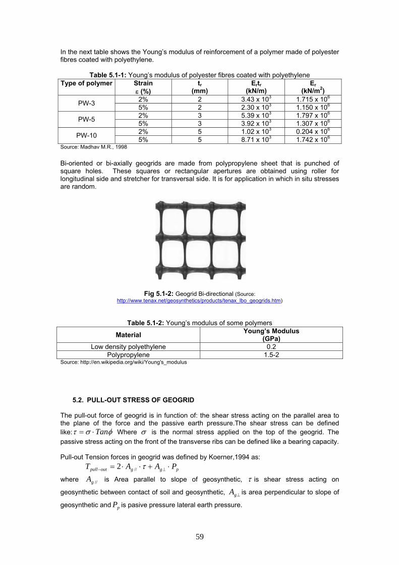
In the next table shows the Young’s modulus of reinforcement of a polymer made of polyester fibres coated with polyethylene.

Table 5.1-1: Young’s modulus of polyester fibres coated with polyethylene Type of polymer

Strain ε (%)

tr (mm)

Ertr (kN/m)

Er (kN/m2)

2% 2 3.43 x 103 1.715 x 106 PW-3 5% 2 2.30 x 103 1.150 x 106

2% 3 5.39 x 103 1.797 x 106 PW-5 5% 3 3.92 x 103 1.307 x 106

2% 5 1.02 x 103 0.204 x 106 PW-10 5% 5 8.71 x 103 1.742 x 106

Source: Madhav M.R., 1998

Bi-oriented or bi-axially geogrids are made from polypropylene sheet that is punched of square holes. These squares or rectangular apertures are obtained using roller for longitudinal side and stretcher for transversal side. It is for application in which in situ stresses are random.

Fig 5.1-2: Geogrid Bi-directional (Source: http://www.tenax.net/geosynthetics/products/tenax_lbo_geogrids.htm)

Table 5.1-2: Young’s modulus of some polymers

Material Young’s Modulus (GPa)

Low density polyethylene 0.2 Polypropylene 1.5-2

Source: http://en.wikipedia.org/wiki/Young's_modulus

5.2. PULL-OUT STRESS OF GEOGRID The pull-out force of geogrid is in function of: the shear stress acting on the parallel area to the plane of the force and the passive earth pressure.The shear stress can be defined like: φστ Tan⋅= Where σ is the normal stress applied on the top of the geogrid. The passive stress acting on the front of the transverse ribs can be defined like a bearing capacity. Pull-out Tension forces in geogrid was defined by Koerner,1994 as: pggoutpull PAAT ⋅+⋅⋅= ⊥− τ//2

where is Area parallel to slope of geosynthetic, //gA τ is shear stress acting on

geosynthetic between contact of soil and geosynthetic, is area perpendicular to slope of

geosynthetic and is pasive pressure lateral earth pressure. ⊥gA

pP

59

The same formula can be expressed in the following equation: ( ) ( ) obSstensiongeogrid qTRTRLRF ⋅+⋅+⋅= ∑∑ ∑− τ2

Where is Total pullout strength, is the longitudinal rib area and is

Transverse rib area of shear strength, is transverse rib area of bearing strength and is the bearing capacity and

tensiongeogridF − SLR STR

oqbTRτ is Shear stress.

Fig 5.2-1: Pull-out stress of geogrid (Source: Diagram from Koerner, 1994)

The pull-out mechanism of geogrid is provided by two main components like: - The frictional resistance offered by the longitudinal member of the geogrid or

longitudinal or transverse areas of ribs. - The passive bearing resistance offered by the transverse members of the geogrid.

The total pull-out forces is defined by the following equation:

bfoutpull TTT +=−

Where: : Frictional forces fT

bT : The passive bearing force The frictional force is formulated using Moht-Coulomb criterion:

( ) ATanCAT anaff 22 ⋅⋅+=⋅= δστ

Where: fτ : The actual frictional resistance

: The actual adhesion intercept, aC nσ : The confining pressure,

aδ : The friction angle between soil and geosynthetic,

: The embedded area of the geosynthetic AThe passive bearing force of the transverse members is in function of cohesion, friction angle and the bearing capacity factors in the Terzaghi-Buisman bearing capacity equation, which was modified like the following equations:

By Peterson and Anderson, 1980: ( )qvcb NCNdwnT ⋅+⋅⋅= σ

By Bergado and Anderson, 1992:

( )NCdwnT ⋅⋅= cub

Where: n : the number of transverse members

w : the width of the reinforcement d : the thickness of the transverse members of the geogrid

60

⎟⎠⎞

⎜⎝⎛ +⋅=

2452 φφπ TaneN Tan

q

2 452

Tan

qN e Tanπ φ φ φ⎛ ⎞+ ⋅⎜ ⎟⎝ ⎠ ⎛ ⎞= +⎜ ⎟

⎝ ⎠

( )1−⋅Φ= qc NCotN

Φ⋅+= TanCC nu σ Where: C : the cohesion intercept (obtained from direct shear test) nσ : the confining pressure Φ : the soil friction angle

5.3. SHEAR STRESS OR COHESION DUE TO GEOGRIDS INTO THE SOIL The geogrid lied down on the inner slope will have an additional tension produced by the shear water stress. It is additional tension since the geosynthetic have a previous tension during the installation. This distributed shear stress will make that the soil distorted an angle ω and if we assumed that the geosynthetic-root-soil behaves like a rigid body, the geogrid will rotate an angle ω . This angle could be represented like a distributed moment produced

by distributed shear water stress located at distance above the geosynthetic. 0M

DThis distributed moment will generate a traccional stress tσ at point c of the geosynthetic

that is equal to geogrid

geogridt I

yM ⋅=σ where M is the moment produced in the geogrid by

distributed moment, the inertia of geogrid is 3' eb ⋅121⋅=I geogrid

m1

( ' is the sum of all widths of

tranverse rib of geogrid in a width of b

b

= , and is the thickness of geogrid) and e

2eygeogrid =

T

ω

ω

Fig 5.3-1: Distortion of geogrid due to shear stress of water

61

The shear water stress in 1m of transversal length of dike will produce a distributed moment , this is 0M DM wo ⋅= τ where shear water stress is the hIww ⋅⋅= γτ and water depth is

. DTo calculate M at any point , the geogrid of length L, thickness and base b’ is modeled as a beam on elastic foundation with distributed moment acting on it. See Fig.5.3.2.

is in the clockwise direction, is the point where moment is required, is the length of

geogrid before point and is the length of geogrid after point .

c

b

eoM

oM c ac c

L

oM

c

ba

Fig 5.3-2: Beam lies down on elastic foundation under load of distributed moment

Based on this mathematical model mentioned above, the angle and moment produced at point in the geogrid lied down on slope is defined as: c

( )bSineaSinek

M bac λλ

λω λλ −− ++−

⋅−= 2

20

( ) ([ ]bCosbSineaCosaSineM

M baoc λλλλ

λλλ −+−+−

−= −−2

4)

44 geogridgeogrid IE

k⋅

=λ

where is the modulus of geosynthetic, is the modulus of foundation per unit width,

is the distance from the top of the dike to point in analysis located downward at slope. is the longitude of the dike slope minus distance a .

geogridE

a−

kca

b L= LThe maximum tσ is in the top of geosynthetic section so the distance from the top to neutral

axis of geosynthetic beam is 2eygeogrid = . The tension at point is c gtc AT

c⋅= σ where

is the sectional area of geogrid. ebAg ˆ'⋅=

Replacing values we have that ggeogrid

cc A

IyM

T ⋅−

=

or ( ) ( )[ ] ggeogrid

baoc A

IybCosbSineaCosaSine

MT ⋅⎥⎦

⎤⎢⎣⎡ −+−+−−

= −− λλλλλ

λλ24

Using the model of Jewell (1980) about the shear stress on reinforced soil we have that the cohesion in the soil due to geogrid is:

)( 'sgicgeosynthet TgCosSinTC φθθ ⋅+⋅=Δ

62

The additional cohesion at point is: c

)( 'scc

s

g

geogrid

cgeogrid TgCosSin

AA

IyM

Cc

φθθ ⋅+⋅⋅⋅

=Δ

And using the model a beam with a simple support- fixed support

( ) ( )[ ] )(ˆ

624

'scc

s

baogeogrid TgCosSin

AebCosbSineaCosaSine

MC φθθλλλλ

λλλ ⋅+⋅

⋅⎥⎦⎤

⎢⎣⎡ −+−+−−

=Δ −−

Where cc ωθ −= 090 The cohesion depends of the material properties of geogrid. The vertical forces like weight of soil and water have been neglected in this model to calculate . gTAccording this model the moment present in the geogrid could vary according of the position of point in analysis. If have high values the additional cohesion produced by geogrid into soil due to shear water stress can be expressed like:

c ba,

⎥⎥⎦

⎤

⎢⎢⎣

⎡⋅⎟⎟⎠

⎞⎜⎜⎝

⎛ ⋅⋅−+⎟⎟

⎠

⎞⎜⎜⎝

⎛ ⋅⋅−⋅

⋅⋅⎥⎦

⎤⎢⎣

⎡=Δ '

20

20 2

22

2ˆ3

ss

ogeogrid Tg

kM

Cosk

MSin

AeM

C φλπλπ

λ

ssr φφ ≈' : the inner friction angle of soil-root is similar to inner friction angle of soil (Hänner, 1991). It means that this model is valid for revetment with geogrid and for grass revetment with geogrid. For instance the cohesion due to geogrid will be calculated for the following values:

26 /10797.1: mkNxEgeogrid , , , 2/280 mkNk = mmegeogrid 3:ˆ mb 28.0'= , ,

, , h ,

mD 30.0=028' =sφ 3:1=I 30.0= m mL 32= , , 21m= 10w =γAs

3/ mkN so it has:

4106 −⋅=geogridI , , 1769.15 −= mλ mmkNM o /3.0 ⋅=

( ) 0≈−− aCosaSine a λλλ for 320 ≤≤ a and

( ) 0≈−− bCosbSine b λλλ for 320 ≤≤ b The values shows above are not depend of position of since those products are almost zero so the equation can be expressed like:

c

( ) 02

0 5.302 =⇒−⋅−

= ωλ

ωk

Mand 05.59=θ

13.1)( ' =⋅+ sTgCosSin φθθ

[ ] 2/5.2113.1ˆ

624

mkNCAe

MC geogrid

s

ogeogrid =Δ⇒⋅

⋅⎥⎦

⎤⎢⎣

⎡−

−=Δ

λ

Thus the additional cohesion produced by geogrid only due to presence of shear water force according equation above is 21.5kN/m2, for any point along the slope. Values of a and b have not influence in the results.

63

5.4. GEOCELLS CHARACTERISTICS

A geocell is a three-dimensional geosynthetic used for reinforcement in the soil. It has the shape of a honeycomb or hexagonal cells that are linked together when it is expanded and it can be transported and stocked in a very compact form. It is resistance to tensile forces and its webs can expand or collapse like accordion. It is made from polyethylene using a single continuous extrusion process. Once it is expanded on the soil surface the cells become dimensionally stable and provide an effective confinement for loose materials placed in each single web. Geocells provides soil confinement without movement even on very steep slopes or with dragging forces like in a stream flow.

Fig 5.4-1: Variable expansion of the geocell

In the next table some characteristics of dimension of typical geocell are shown. These geocells are manufactured by Geoweb System.

Table 5.4-1: Specification of three-dimensional geocell confinement of Geoweb System

Nominal dimensions Type

Nominal Area (cm2)

Length (mm)

Width (mm)

Strip thickness

(mm)

Nominal cell depth

(mm) Material composition

GW20V 289 224 259 GW30V 460 287 320 GW40V 1206 475 508

1.27 75, 100, 150, 200

Polymer-Polyethylene with density 0.935-0965 gr/cm3

Source:http://www.alcoa.com/alcoa-geo/catalog/applications/Geoweb%20General/geoweb_material_specification.pdf

5.5. VERTICAL AND HORIZONTAL STRESS IN THE GEOCELLS The geocell confine the soil improving granular soil shear strength. The shear strength between geocell wall and granular soil is defined below. This effort is a react due to a pressure force that is different to our case, but only it would be to mention since a cohesive strength between the walls of geocell and soil must be considered in this calculation.

Fig 5.5-1: Bearing capacity failure mechanisms of sand with geocell (Source: Diagram from Koerner, 1994)

64

δστ Tanhgeocell ⋅= ; ah Kp ⋅=σ ; ⎟⎠⎞

⎜⎝⎛ −=

2452 φTanKa

geocellτ : Shear strength bewteen geocell wall and soil contained within it.

hσ : Average horizontal force within the geocell

p : Applied vertical pressure, for a unit width is ( ) αγγ CoshDp wsat ⋅⋅+⋅=

aK : Coefficient of active earth pressure

δ : Angle of shearing resistance (friction angle) between soil and the cell wall material (100-300 between sand and smooth or textural geomembranes) Replacing values in the equation, the new relation is:

( ) δφαγγτ TanTanCoshD wsat ⋅⎟⎠⎞

⎜⎝⎛ −⋅⋅⋅+⋅=

2452

For instance it will be calculated the shear strength between geocell wall and soil contained within it, so the following values will be analyzed:

md 30.0= , , or , 028'=φ 3:1=I 04.18 mh 30.0= , mL 32= , ,

, , geocell type GW20V and depth

21mAs =

mm753m satγ/10kNw =γ 3/17kN= m so it has:

( ) 20 /7.7)4.18(30.01030.017 mkNCosp =⋅×+×=

36.02

28450

02 =⎟⎟⎠

⎞⎜⎜⎝

⎛−= TanKa

2/8.236.07.7 mkNh =×=σ 20 /1208.2 mkNTan =⋅=τ

This shear stress (τ ) is around the wall of the cell so if this stress is distributed around the soil, it must be multiplied by an area factor

( ) 22

222

/22895141

2895.79.254.222

1 mkNcmcm

AA

cell

cellwallcellsoil =×=

×+×== −

− τσ

The cell of geosynthetic lied down under a layer of soil with a flow water running over it are undergone to horizontal stress produce by pressure pore and active earth pressure.

water

p ressure d iagram

so il

geocells

γ

γ

γ γ

γγ

σ

σ

σ σσσ σ

Fig 5.5-2: Pressure pore and active earth pressure acting on wall of geocell

65

The upper of geocell has an active earth pressure equal to ( ) DK wsata ⋅−⋅= γγσ '1 where

'1'1

φφ

SinSinKa +

−= , the specific weight of saturated soil is satγ and the water is wγ and the

thickness of soil layer is . It has also a pressure pore equal to D ( )Dhu w +⋅= γ1 , where h is the depth of the water. So the total pressure that produces in the upper is

( ) ( DhK wwsata +⋅⋅−⋅= )D + γγγσ 1 The horizontal pressure in the lower of geocell is

( ) ( ) ( )eDheDK wwsata ++⋅++⋅−⋅= γγγσ 2 It would be consider the average of the horizontal stress acting on the geocell:

2

21 σσσ

+=

Replacing values in the equations we have that σ is equal to:

( ) ( ) ( )22eDheKDK wwwsatawsata ⋅+++⋅−+⋅−= γγγγγγσ

The simplified formula is:

( ) ⎥⎦⎤

⎢⎣⎡ ++⋅+⎥⎦

⎤⎢⎣⎡ +⋅−=

22eDheDK wwsata γγγσ

5.6. SHEAR STRESS OR COHESION DUE TO GEOCELLS INTO THE SOIL The geocell lied down on slope is also anchored each certain distance. Unlike geogrid, a distortion in the soil would not generate a rotation in the geocell since it has more thickness. The layer of geocell fills with soil acts more rigid over drag or shear water stress in such way there is not deformation when the distortion angle appears. What is generated in a geocell is a unit deformation ε due to tension force acting on this geosynthetic. This tension force is applied in situ before putting a cover layer of soil in the geocell. Since the strips of geocell makes an angle with the soil transversal section in analysis, the component of this unit deformation

geoT

Cosε η ε= ⋅ is absorved by the soil. This unit deformation tries to compress the soil and it will be uniformly under the assumption that the soil is isotropic material and obey the law of Hooke.

F

TA

T

εη=ε cos

ε

η

η

=ε

ε

ε

ηcosε

ε

A

E

E

ε

Fig 5.6-1: Unit deformation of the soil with geocell

66

According Hooke’s law the unit deformation in the geocell and soil can be expressed in function of their modulus of elasticity like:

geocellgeocell

geo

AECosT⋅

⋅=

ηε

soilsoil

soil

AEF⋅

=ε

And applying the relation between geocell and soil unit deformation η

εεCos

= , the force

acting on the soil due to the tension applied in the geocell is

η2CosTAEAE

F geogeocellgeocell

soilsoilsoil ⋅⋅

⋅⋅

=

So the compression stress 3σ ,defined like stress parallel to surface, what is acting on the soil

is ησσ 211 Cos

AT

EE

AF

geocell

geo

geocell

soil ⋅soil

soil ⋅=⇒=

And 03 ≅= waterWσ defined like vertical compression stress equal to the weight of water so

0=3σ . Thus 1σ is the maximum stress and 3σ is the minimum stress. With this information it is possible to estimate the failure shear stress using the Coulomb’s law in soil.

'snf Tanc φστ ⋅+= where ( ) ⎟⎠⎞

⎜⎝⎛ +⋅−+= 02

313 452

'sn Cos φσσσσ

Replacing the values of 1σ and 3σ , the new nσ

ηφσ 202 452

' CosCosAT

EE s

geocell

geo

geocell

soiln ⋅⎟

⎠⎞

⎜⎝⎛ +⋅⋅=

The failure shear stress of soil revetment with geocell can be defined as:

'202 452

's

s

geocell

geo

geocell

soilf TanCosCos

AT

EE

c φηφ

τ ⋅⋅⎟⎠⎞

⎜⎝⎛ +⋅⋅+=

If we compare this model based with Jewell’s model (1980) about the shear stress in the reinforced soils, we have that the additional cohesion in the soils reinforced with geocell is:

)( 'sgicgeosynthet TgCosSinTC φθθ ⋅+⋅=Δ

And under the assumption that the failure plane is parallel to surface so 090θ = the additional cohesion in the geocells is defined as:

geogeosynthetic g geosynthetic

s

TC T C

AΔ = ⇒ Δ =

So it could be conclude that there is two ways how to define the additional cohesion produced by the geocell into the soil. The model of Jewell will be used in this thesis, the other model proposed in this item is only referential. For instance if we have a soil sand greatly silty clayey where,

, , and geocell type GW20V, so with 20soil

E M= Pa 0' 25=sφ 0c = 06.24=η

67

0.20geocell

E = MPa , thickness and depth of geocell is 1.27mm and 75mm respectively and

applying a tensional stress of 1geo

geocell

TMPa

A= , the failure shear stress is:

02000

2 6.2425452

251.2.0

20 CosTanCosMPaMPaMPa

f ⋅⋅⎟⎟⎠

⎞⎜⎜⎝

⎛+⋅⋅=τ

MPaf 12.11=τ The previous model only define the shear stress for soil with geocell, but if the soil has root the additional cohesion produce by the root has to be included in the shear stress. Like

: the inner friction angle of soil-root is similar to inner friction angle of soil (Hänner, 1991), so the failure shear stress of root revetment with geocell can be defined as:

ssr φφ ≈'

rootrssr

geocell

geo

geocell

soilf CTanCosCos

AT

EE

c Δ+⋅⋅⎟⎠⎞

⎜⎝⎛ +⋅⋅+= '202 45

2'

φηφ

τ

Replacing the model of O’Loughlin (1982), the new equation for the failure shear stress of root revetment with geocell is:

AATTanCosCos

AT

EE

c RRrs

sr

geocell

geo

geocell

soilf ⋅⋅+⋅⋅⎟

⎠⎞

⎜⎝⎛ +⋅⋅+= 2.145

2' '202 φη

φτ

5.7. STABILITY OF COVER SOIL ON GEOMEMBRANE LINED SLOPES Koerner and Hwu, 1991, defined a model about cover soil stability on side slopes when placed above a geomembrane. The method used to analyze stability is based on the isolation of free body diagrams. Since the plane of failure is clearly defined at the contact between the soil and geomembrane is easy to apply free body diagrams. Two-part wedge method is utilized and it is developed the free body diagrams for each one introducing safety factors for

friction angles between geomembrane-soil (FSDδδ = ), between soil-soil (

FSS

Dφ

φ = )and

cohesion forces between geomebrane-soil ( LFSc

C aA ⋅= ) and soil-soil (

ωSinD

FScC p ⋅= ).

Active wedge and passive wedge is defined in the equilibrium analysis. The active wedge tends to expand while the passive wedge tends to compress. There are interactive forces acting between each other that they need to be similar to keep in equilibrium state the wedges ( ). When the active wedge tries to expand and press the passive wedge to move in imminent failure state, the soil pressure disappears in the top of the active wedge. See Fig.5.7.1

pa EE =

68

αφ

γ φ

δ

Fig 5.7-1: Pasive and active wedge with forces involves in free diagram body of

a cross-section of cover soil on a geomembrane (Source: Koerner & Hwu, 1991)

The free body diagram for passive wedge is developed taking account forces as the weight ( ) , the pressure soil ( ), the soil reaction ( ) and the cohesion ( ). Similar forces for active wedge are used but the sub-index in the nomination changes. The respective equilibrium of forces is shown in Fig.5.7-2.

pW pE pF pC

φ

α

α

δ αα

φ α

δ

α

αα

α

Fig 5.7-2: Diagram of free body for passive and active wedge of cover soil on a geomembrane

(Source: Koerner & Hwu, 1991) This method calculates a formula that defines the Security Factor ( )FS

ac avoiding failure in

function of: cohesion between soil-soil ( ) and geomembrane-soil ( ), also friction angle

between soil-soil (

cφ ) and geomembrane-soil (δ ), angle of slope (α ), thickness of soil layer

( ), length of the layer in analysis ( ), and specific weight of soil (D L sγ ). The equilibrium of foces acting on both wedges makes that security factor be a second degree equation. That is shown in the next equation derivate by Koerner and Hwu, 1991.

69

( ) ( ) ( )2 2 2( ) 0.5 2 [ 2s sFS LD Sin FS LD Cos Tan Sinγ α γ α δ⎡ ⎤⋅ ⋅ − ⋅ ⋅ ⋅⎣ ⎦ α

( ) ( )22 2a s sc LCos Sin LD Sin Tan Sinα α γ α φ α+ + ⋅ ⋅ 22 ] [(s s scDCos D Tan LD Cos Tanα γ φ γ α+ + + ⋅ ⋅ δ

] 0

( )( )) 2a sc L Tan Sin Sinφ α α+ = 2 0ax bx c+ + =

( )20.5 2sa LD Sinγ α= ⋅ ⋅

( ) ( )2[ 2s ab LD Cos Tan Sin c L Cos Sin 2γ α δ α α α= − ⋅ ⋅ ⋅ + ⋅ ⋅

( )2 22 2 ]s s sLD Sin Tan Sin cDCos D Tanγ α δ α α γ φ+ ⋅ ⋅ + +

( ) ( )( )2s a sc LD Cos Tan c L Tan Sin Sinγ α δ φ α α= ⋅ ⋅ +

2 42

b b acFSa

− ± −=

5.8. REQUIRED TENSILE STRENGTH OF GEOGRID REINFORCEMENT OF COVER SOIL ON AN GEOMEMBRANE

When the security factor is less than one, reinforcement is needed to add into the soil layer located on a geomembrane. In this case the pressure that exerts the active wedge against passive wedge is higher that the pressure exerted by passive wedge that is to say:

pA EE ≥

Thus the geogrid gives the additional tensional force (T ) that is needed to keep in equilibrium the system and it is defined as:

Ap ETE =+ ⇒ pA EET −=

α

γ φ

T

Fig 5.8-1: Geogrid reinforcement of cover soil on geomembrane

(Source: Koerner & Hwu, 1991) To define the reaction forces between active and passive wedge is necessary to have the safety factor equal to one since in this state it can verify if the active wedge tends to move the passive wedge. Besides it should be taken account that the friction angle is just the soil.

1=FS ⇒ δδ =D SD φφ = LcC aA ⋅= αSin

DcC p ⋅=

Using the free body diagrams, the pressures or reactive forces are defined as:

70

( )A

D

DsA C

CosSinLD

E −−⋅⋅

=δ

δαγ

( )αφ

φα

γα

φ

+

⎥⎦

⎤⎢⎣

⎡⋅

⋅+⋅⋅

=D

Ds

D

p Cos

TanSin

DSin

DFSCCos

E2

2

Replacing these values, the tension exerted in the geogrid (T ) is:

( )( )αφ

φα

γα

φ

δδαγ

+

⎥⎦

⎤⎢⎣

⎡⋅

⋅+

⋅⋅

−−−⋅⋅

=Cos

TanSin

DSin

DCCosC

CosSinLD

T

s

As 2

2

5.9. STABILITY OF GRASS REVETMENT DURING AN OVERTOPPING EVENT USING KOERNER METHOD

In this item, it will be applied the same criterion of Koerner method to analyse the safety factor of a grass revetment during an overtopping event. The additional forces that are taken account in this static model are the root shear force ( )rootCFΔ and water shear force . The revetment will be divided in two wedges for apply equilibrium.

( )wFτ

αφ

γ φ

δΔ

Δ

τ

τ

Fig.5.9-1: Forces acting on active and passive wedges of grass revetment during an overtopping event

The forces taken account in the passive and active wedges are:

Table 5.9-1: Forces acting on the passive and active wedge of grass revetment during an overtopping event

71

Forces Passive wedge Active wedge

Weight of soil α

γ2

2

SinD

W satS p

⋅= LDW satS A

⋅⋅= γ

Weight of water α

γ2

2Sin

DhW w

W p

⋅⋅⋅= LhW wWA

⋅⋅=γ

Shear water force α

γτ Cos

DhF w

wp

⋅⋅= LhSinF wwA

⋅⋅⋅= αγτ

Root-soil cohesion force αSin

DFS

CCC roots

p ×Δ+

= LFS

CCC rootS

A ×Δ+

=

Pressure forces pE AE Reaction force pF AF

The safety factor is applied to cohesion force and friction angle of soil-root

FSTanTan sr

D

'φφ = and

FSTanTan D

δδ =

It is expected that δφ ='sr since they are the friction angle of the soil-root matrix, however tests are needed to confirm that due to position of the failure plane.

α α α

α

Δα

φ

Δ

τ

τ

α

φ

Fig.5.9-2: Forces acting on passive wedges of grass revetment during an overtopping event

Applying the equilibrium in the force polygon of passive wedge (See Fig.5.9-2), the following relations are obtained:

:yFΣ DppwWS CosFSinESinFWWppp

φαατ =+++

:xFΣ ααφ τ CosECosFSinFC ppwDpp +=+ The pressure acting on the passive wedge is obtained like:

( )( )D

wwWSDpp

TanSinCos

CosFSinFWWTanCE pppp

φαα

ααφ ττ

−

−+++=

This pressure in function of safety factor is:

⎟⎠⎞

⎜⎝⎛ ⋅−

⋅⋅−⎟⎟

⎠

⎞⎜⎜⎝

⎛ ⋅⋅+

⋅⋅⋅+

⋅+×

Δ+

=

FSTanSinCos

CosCos

DhSinCos

DhSin

DhSin

DFS

TanSin

DFS

CC

E

wwwsatsrroots

pφαα

αα

γαα

γα

γα

γφα 2

22

' 2

Applying the equilibrium in the force polygon of active wedge (See Fig.5.9-3), the following relations are obtained:

:yFΣ ( ) ( )AA WSAwDAAA WWSinFSinFSinCE ++⋅=+−⋅+⋅+ αδαα τ

090

72

:xFΣ ( ) ( )DAAwAA CosFCosFCosCE δααα τ +−⋅+⋅=⋅+ 090 The pressure acting on the active wedge is obtained like:

( )( ) αδατ CosTanTanWWCFE DWSAAwAAA

⋅−++−=

( ) αδαγγαγ CosFS

TanTanLhLDLFS

CCLhSinE wsat

rootSwA ⋅⎟

⎠⎞

⎜⎝⎛ −⋅⋅+⋅⋅+×

Δ+−⋅⋅⋅=

δ ααΔ

α

Δ

α

τ

τ

δ

Fig.5.9-3: Forces acting on active wedge of grass revetment during an overtopping event

For to calculate the safety factor the pressure forces acting on the passive and active wedges are equal.

Ap EE = The safety factor is calculated solving the following quadratic equation:

( )( )( )

( )( )( )( )

( )( ) 0

22

22

2

2

2

=⋅++⋅Δ⋅+

⋅

⎥⎥⎥⎥⎥

⎦

⎤

⎢⎢⎢⎢⎢

⎣

⎡

+++

⋅++⋅Δ+

++⋅⋅+×Δ

−⋅⎥⎦⎤

⎢⎣⎡ +++

δαφα

αφα

δαα

αφα

αα

τ

τ

ττ

TanCosWWLCTanSin

FS

SinWWFTanSin

TanCosWWLCSin

SinFWWTanSinDC

FSSinWWFFSin

AA

AA

AA

ppp

AAp

WSt

WSAw

WSt

wWSt

WSwAw

( )( )ααττ SinWWFFSina

AAp WSwAw +++=22

( )⎟⎠⎞

⎜⎝⎛ ⋅+⋅⋅⋅+⋅⋅⋅= hDLSinDhSina wsatw γγαγα 22

21

73

( ) ( )( )( )( ) ⎥

⎥⎥

⎦

⎤

⎢⎢⎢

⎣

⎡

+++

⋅⋅++⋅Δ+++⋅+×Δ−=

αφα

δαααφα

τ

τ

SinWWFTanSin

TanCosWWLCSinSinFWWTanSinDCb

AA

AAppp

WSAwsr

WStwWSsrt

'22'

2

( )

( )( )

( )⎥⎥⎥⎥⎥⎥⎥

⎦

⎤

⎢⎢⎢⎢⎢⎢⎢

⎣

⎡

⋅⋅+⋅⋅⋅+

⋅⋅⋅+⋅+Δ⋅⋅+

⎟⎠⎞

⎜⎝⎛ +⋅⋅+

⋅⋅+×Δ

−=

hDLTanSin

CosTanhDCLSin

SinhD

CosTan

DDC

b

wsatsr

wsatt

wsatsr

t

γγφα

αδγγα

αγγ

αφ

2'22

12

'

3

2

( )( )[ ]δαφα TanCosWWLCTanSincAA WStsr ⋅⋅++⋅Δ⋅⋅= '2

( )( )[ ]δαγγφα TanCoshDCLTanSinc wsattsr ⋅⋅⋅+⋅+Δ⋅⋅⋅= '2

2 0ax bx c+ + = or 02

=+⋅+⋅ cFSbFSa

aacbbFS

242 −±−

=

If 1≥FS , the system is in equilibrium. It means the grass revetment during a overtopping event does not need reinforcement.

5.10. TENSILE STRENGTH OF GEOSYNTHETIC REINFORCEMENT OF GRASS REVETMENT

If safety factor of grass revetment during overtopping event is 1<FS , it is needed a reinforcement in the grass revetment. Thus the tension produced in the geosynthetic is the difference between active and passive pressure with a safety factor equal to one.

Ap ETE =+ ⇒ pA EET −=

α

γ φ

T

Fig.5.10-1 : Geosynthetic reinforcement of grass revetment during an overtopping event

The active and passive pressure will be redefined for safety factor equal one. The following relations are obtained: For 1=FS

74

( ) ( )( ) αδαγγαγ CosTanTanLhLDLCCLhSinE wsatrootSwA ⋅−⋅⋅+⋅⋅+×Δ+−⋅⋅⋅=

( ) ( ) ( ) LCCLhSinCos

SinhDLE rootSw

wsatA ×Δ+−⋅⋅⋅+

−⋅⋅+⋅⋅= αγ

δδαγγ

( )

( )'2

22

'2

sr

wwwsat

srroots

pTanSinCos

DhSinCos

DhSin

DhSin

DTanSin

DCCE

φαα

γαα

γα

γα

γφ

α⋅−

⋅⋅−⎟⎟⎠

⎞⎜⎜⎝

⎛ ⋅⋅+

⋅⋅⋅+

⋅+×Δ+

=

( ) ( )( )

( )⎥⎥⎥⎥

⎦

⎤

⎢⎢⎢⎢

⎣

⎡

+

⋅−+⋅⋅+⋅+Δ+

⋅⋅='

122

'

'

2

sr

wwsatsrroots

srpCos

hSinhDSinTan

SinCC

DCosEφα

γαγγαφ

αφ

Thus the tension in the grass revetment with overtopping event is ( it means ): 0≠h

( ) ( ) ( )

( )( ) ( )( ) ⎥

⎦

⎤⎢⎣

⎡⎟⎠⎞

⎜⎝⎛ ⋅−+⋅⋅+⋅+

Δ+⋅

+⋅

−

⎥⎦⎤

⎢⎣⎡ ×Δ+−⋅⋅⋅+

−⋅⋅+⋅⋅=

hSinhDSinTan

SinCC

CosDCos

LCCLhSinCos

SinhDLT

wwsatsrroots

sr

sr

rootSwwsat

γαγγαφ

αφαφ

αγδ

δαγγ

2122

''

'

The tension in the grass revetment without overtopping event is (it means ): 0=h

( ) ( ) ( )( )

( )⎥⎥⎥⎥

⎦

⎤

⎢⎢⎢⎢

⎣

⎡

⎥⎥⎥⎥

⎦

⎤

⎢⎢⎢⎢

⎣

⎡

+

⋅⋅+Δ+

⋅⋅−⎥⎦⎤

⎢⎣⎡ ×Δ+−

−⋅⋅⋅=

'2

'

'sr

ssrroots

srrootSs

Cos

DSinTan

SinCC

DCosLCCCos

SinDLTφα

γαφ

αφδ

δαγ

The tension has to be positive so it is necessary that slope angle is higher than friction angle of root-soil matrix ( δα ≥ ). But 'srφδ ≅ and some tests made in root-soil matrix shows that

the range of [ ]040025 −'=srφ . Besides ( ) ( )31tan5.2

1tan ArcArc −=α or

[ ]00 2218 −=α . It means that δα < thus the tension will be negative, for this reason the angleδ have to be investigated. This is out of this thesis. In general the tension can be expressed like where safety is equal to one ( 1=FS ):

( )( )[ ]( )( ) ⎥

⎥⎦

⎤

⎢⎢⎣

⎡

−

−+++−

⋅−++−=

D

wwWSDp

DWSAAw

TanSinCos

CosFSinFWWTanC

CosTanTanWWCFT

pppp

AA

φαα

ααφ

αδα

ττ

τ

75

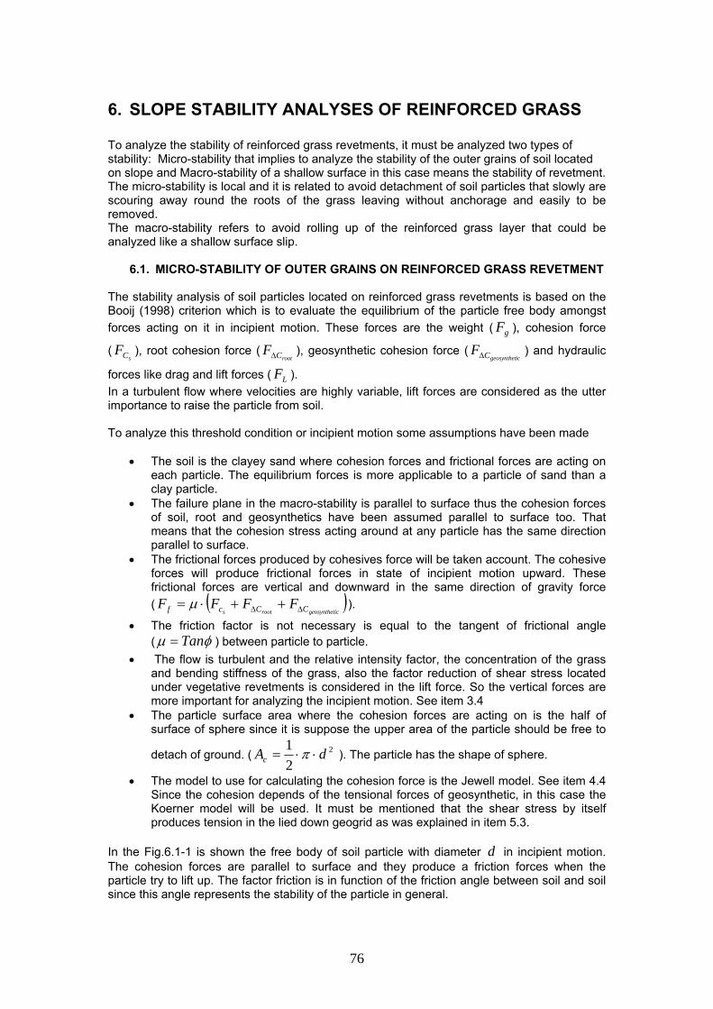
6. SLOPE STABILITY ANALYSES OF REINFORCED GRASS To analyze the stability of reinforced grass revetments, it must be analyzed two types of stability: Micro-stability that implies to analyze the stability of the outer grains of soil located on slope and Macro-stability of a shallow surface in this case means the stability of revetment. The micro-stability is local and it is related to avoid detachment of soil particles that slowly are scouring away round the roots of the grass leaving without anchorage and easily to be removed. The macro-stability refers to avoid rolling up of the reinforced grass layer that could be analyzed like a shallow surface slip.

6.1. MICRO-STABILITY OF OUTER GRAINS ON REINFORCED GRASS REVETMENT The stability analysis of soil particles located on reinforced grass revetments is based on the Booij (1998) criterion which is to evaluate the equilibrium of the particle free body amongst forces acting on it in incipient motion. These forces are the weight ( ), cohesion force

( ), root cohesion force ( ), geosynthetic cohesion force ( ) and hydraulic

forces like drag and lift forces ( ).

gF

geosynthetsCFrootCFΔ

LFicCFΔ

In a turbulent flow where velocities are highly variable, lift forces are considered as the utter importance to raise the particle from soil. To analyze this threshold condition or incipient motion some assumptions have been made

• The soil is the clayey sand where cohesion forces and frictional forces are acting on each particle. The equilibrium forces is more applicable to a particle of sand than a clay particle.

• The failure plane in the macro-stability is parallel to surface thus the cohesion forces of soil, root and geosynthetics have been assumed parallel to surface too. That means that the cohesion stress acting around at any particle has the same direction parallel to surface.

• The frictional forces produced by cohesives force will be taken account. The cohesive forces will produce frictional forces in state of incipient motion upward. These frictional forces are vertical and downward in the same direction of gravity force ( ( )

icgeosynthetroots CCcf FFFF ΔΔ ++⋅= μ ).

• The friction factor is not necessary is equal to the tangent of frictional angle ( φμ Tan= ) between particle to particle.

• The flow is turbulent and the relative intensity factor, the concentration of the grass and bending stiffness of the grass, also the factor reduction of shear stress located under vegetative revetments is considered in the lift force. So the vertical forces are more important for analyzing the incipient motion. See item 3.4

• The particle surface area where the cohesion forces are acting on is the half of surface of sphere since it is suppose the upper area of the particle should be free to

detach of ground. ( 2

21 dAc ⋅⋅= π ). The particle has the shape of sphere.

• The model to use for calculating the cohesion force is the Jewell model. See item 4.4 Since the cohesion depends of the tensional forces of geosynthetic, in this case the Koerner model will be used. It must be mentioned that the shear stress by itself produces tension in the lied down geogrid as was explained in item 5.3.

In the Fig.6.1-1 is shown the free body of soil particle with diameter in incipient motion. The cohesion forces are parallel to surface and they produce a friction forces when the particle try to lift up. The factor friction is in function of the friction angle between soil and soil since this angle represents the stability of the particle in general.

d

76

Fig 6.1-1: Incipient motion of soil particle of reinforced grass revetment

A simple analysis of equilibrium in vertical forces is based on that the upward forces must be equal or lower than downward forces to avoid detachment of the particles. Only vertical forces are consider since in the turbulent flow the velocities are higher so lift forces become important to keep the equilibrium. Making a simple equilibrium amongst vertical forces, this relation must be fulfillment:

1)(≤

++⋅+ ΔΔ icgeosynthetroots CCCg

L

FFFFF

μ

The lift forces are defined as the following relation (Details of this equation and variables are explained in item 3.4).

( )321 222

22282.9a

s

v

a

w

sa

sooL h

HhghIhhMAghIdrF ⎟⎟

⎠

⎞⎜⎜⎝

⎛⋅⎟

⎟⎠

⎞⎜⎜⎝

⎛ ⋅⋅⎟⎟

⎠

⎞⎜⎜⎝

⎛⋅⋅⋅⋅⋅=

ν

The gravity force is defined like the submerged weight of the spherical particle

( ) gdF wsg ⋅−⋅⋅⋅= ρρπ 3

61

The soil cohesion force is more an electronic force between clay particles however in sand is more a pressure force so in an imminent movement, it will produce friction between the contacts of particles. It is defined as:

csC AcFS

×= The root cohesion forces is defined as the simple perpendicular model and simplified but the method of O’Loughlin, 1982. See item 4.2.1 for more details.

crootC ACFroot

×Δ=Δ ⇒ cR

RC AAATF

root×⋅⋅=Δ 2.1

The geosynthetic forces are based on the model made by Jewell, however this model depends on the tension stress acting on the geosynthetic. Koerner defined a model where the tension depends on if the wedge active reaction is higher than the passive wedge reaction of layer revetment. However in the case where these reactions are in equilibrium this tension is zero so cohesion due to geosynthetic does not exist. In the item 5.3 is shown that the tension in the geogrid is not only caused of disequilibrium of these reactions but also the tension appears for the rotation angle produced by water shear stress on geogrid thus in case of equilibrium this tension could be used to estimate the cohesion produced into the soil when the water is running down in the slope. In the case of geocell, there is an elongation that causes the cohesion into the soil and it is in function of tension stress too. In the item 5.4 is explained in detail this model. Jewell model has the following limitations in this model: first the geocell looks a rigid material due to its high thickness so there is not a rotation angle in the geocell and second the failure plane is parallel to surface so so the tension force divided by the soil area parallel to surface is the tension stress that produces cohesion. However the model of Jewell will be used in this analysis of equilibrium motion.

090=θ

77

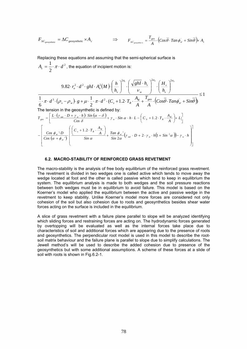
cicgeosynthetC ACFicgeosynthet

×Δ=Δ ⇒ ( ) csrgeo

C ASinTanCosA

TF

icgeosynthet×+⋅⋅=Δ θφθ '

Replacing these equations and assuming that the semi-spherical surface is

2

21 dAc ⋅⋅= π , the equation of incipient motion is:

( )

( ) ( )1

)2.1(21

61

82.9

'23

222222

321

≤+⋅⋅+⋅⋅+⋅⋅⋅⋅+⋅−⋅⋅⋅

⎟⎟⎠

⎞⎜⎜⎝

⎛⋅⎟

⎟⎠

⎞⎜⎜⎝

⎛ ⋅⋅⎟⎟

⎠

⎞⎜⎜⎝

⎛⋅⋅⋅⋅⋅

θφθπμρρπ

ν

SinTanCosA

TAATCdgd

hHhghI

hhMAghIdr

srgeoR

Rsws

a

s

v

a

w

sa

soo

The tension in the geosynthetic is defined by: ( ) ( )

( ) ( )( )⎥⎥⎥⎥

⎦

⎤

⎢⎢⎢⎢

⎣

⎡

⎟⎟⎟⎟

⎠

⎞

⎜⎜⎜⎜

⎝

⎛

⋅−+⋅⋅+⋅+⎟⎠⎞

⎜⎝⎛ ⋅⋅+

⋅+⋅

−

⎥⎦

⎤⎢⎣

⎡×⎟

⎠⎞

⎜⎝⎛ ⋅⋅+−⋅⋅⋅+

−⋅⋅+⋅⋅=

hSinhDSin

TanSin

AATC

CosDCos

LA

ATCLhSinCos

SinhDLT

wwsatsr

RRs

sr

sr

RRSw

wsatgeo

γαγγαφ

αφαφ

αγδ

δαγγ

2122

'2.1

''

2.1

6.2. MACRO-STABILITY OF REINFORCED GRASS REVETMENT The macro-stability is the analysis of free body equilibrium of the reinforced grass revetment. The revetment is divided in two wedges one is called active which tends to move away the wedge located at foot and the other is called passive which tend to keep in equilibrium the system. The equilibrium analysis is made to both wedges and the soil pressure reactions between both wedges must be in equilibrium to avoid failure. This model is based on the Koerner’s model who applied the equilibrium between the active and passive wedge in the revetment to keep stability. Unlike Koerner’s model more forces are considered not only cohesion of the soil but also cohesion due to roots and geosynthetics besides shear water forces acting on the surface is included in the equilibrium. A slice of grass revetment with a failure plane parallel to slope will be analyzed identifying which sliding forces and restraining forces are acting on. The hydrodynamic forces generated by overtopping will be evaluated as well as the internal forces take place due to characteristics of soil and additional forces which are appearing due to the presence of roots and geosynthetics. The perpendicular root model is used in this model to describe the root-soil matrix behaviour and the failure plane is parallel to slope due to simplify calculations. The Jewell method’s will be used to describe the added cohesion due to presence of the geosynthetics but with some additional assumptions. A scheme of these forces at a slide of soil with roots is shown in Fig.6.2-1.

78

α

γ φ

ρ

ΔΔ

τ

Fig.6.2-1: Forces acting on slice of grass revetment due to an overtopping event on inner slope

In this model some assumptions were done: With respect to the soil: The soil is homogeneous and it is composed by sand and clay, it is clayey sand. The plane failure is parallel to surface. The revetment is divided in two slides and free body diagrams are made for both. The soil pressure reaction between them is using wedge method so coefficient methods to estimate these pressure reactions are not applicable in this analysis. With respect to the roots: The additional force given by roots is represented as added cohesion in the shear stress of the soil so tensional forces of roots are not consider in the analysis of this equilibrium.. The failure moment happens when all the roots reach their maximum tensile stress. This maximum tensile stress is reached in all roots simultaneously so this means all roots break at the same time. The maximum tensile stress happens at the same time when the passive wedge and active wedge tends to failure so tensional forces of roots are not zero in the analysis of this equilibrium. The initial position of roots is perpendicular to the slope and they make a distortion angle when they are pulling out. With respect to the flow: The shear stress flow acting on the surface of the slope is estimated like an average boundary shear stress and it is approximated by “depth-slope” product. The water running down on the slope is represented like water flowing in a very wide channel. The slope of the dikes is not so small so it can be not approximated ωω TanSin = . The depth of the water is the same along of the slope so the depth variations due to different velocities whether for laminar flow or turbulent flow are not taken account. The force due to pressure pore will be not taken account. With respect to the geosynthetics: The only geosynthetics considered are geogrid and geocell. The additional force given by geosynthetics is represented as aditional cohesion in the shear stress of the matrix root-soil. The failure plane is parallel to surface in the active wedge and it is in the contact between soil and geosynthetic. In the case of the geogrid, the cohesion is in function of the tensional stress present itself in the geosynthetic. The shear stress between the contact of the geogrid and soil is not taken account in this analysis. This shear stress is defined in function of the tension force or pull-out force in the geogrid, more detail in item 5.2. This shear stress is estimated like:

//2 g

pgoutpull

APAT

⋅

⋅−= ⊥−τ

79

6.3. LOADS PRESENT IN THE STATIC MODEL The loads consider in this static model are shown in Fig.6.3-1.

αφ

γ φ

δ

ΔΔ

ΔΔ

τ

τ

Fig.6.3-1: Forces acting on active and passive wedges of reinforced grass revetment due to an overtopping event on inner slope

Below each force acting on the slice of grass revetment will be described including some assumptions to simplify the analysis.

( )rootCΔ : Shear force of root The effect of the roots into the soil in this static model of the thesis will be represented by one force: A shear force parallel to slope or surface (hypothetical failure plane) that is the product of root cohesion and the length of the slope. A tension force perpendicular to this failure plane similar to anchorages will be not taken account since they are represented by cohesion forces into the soil. The perpendicular root model defined in the item 4.2.1 is going to be used in this thesis. This model explain that roots increase the shear stress of soil due to cohesion increases but it does not say anything about the behaviour of the normal stress to failure plane. However this component will be not taken account in this thesis. According to this model the root shear stress is defined as:

[ ]θφθ SinTanCosAATC sr

RRroot +⋅⋅=Δ '. or

AATC R

Rroot ⋅⋅=Δ 2.1

Where: θ : Angle of shear distortion respect to a plane parallel to slope between [ ]00 9040 −

'srφ : Angle of internal friction soil-root [ ]00 4025 −

AAR : Root area ratio or RAR (no units). is area of the root crossing the shear area and

is total cross-sectional area of shear plane. It must be in the order of 0.25% (Msc. Thesis Young M., 2005)

RA

A

RT : The tensile strength of the roots. (grasses and herbs: 0 – 25 MPa ( Coppin and Richards 1990)

rootCΔ : Additional cohesion due to roots in the soil. [1-20Kpa (O’Loughlin, 1982)]

80

In the active wedge, this root shear force parallel to slope or surface of a unit width and length slope of is represented by: L L

AA

TCf RRroot A

⋅⋅⋅=Δ 2.1

In the passive wedge, this root shear force is horizontal and it is present only in the horizontal failure plane. For a unit width, it is represented by:

αSin

DAATCf R

Rrootp⋅⋅⋅=Δ 2.1

The safety factor is considered in these resistant forces.

⎟⎠⎞

⎜⎝⎛ ⋅⋅⋅=Δ L

AA

TFS

CF RRroot A

2.11 and ⎟⎠⎞

⎜⎝⎛ ⋅⋅⋅=Δ

αSinD

AA

TFS

CF RRroot p

2.11

Shear Force of clay- sand soil ( )sC :

This force refers to the cohesion in the soil ( )sC produced by the presence of clay. This cohesion varies between 0-2 KPa for a clay greatly sandy soil (See item 4.1.2). In the active wedge, this cohesion shear force parallel to slope or surface of a unit width and length slope of is represented by: L LCfC SS A

⋅=

In the passive wedge, this cohesion shear force is horizontal and it is present only in the horizontal failure plane. For a unit width, it is represented by:

αSinDCfC SS p

⋅=

The cohesion force in the contact between the wedges is not taken account since the cohesion is a shear stress. The safety factor is considered in these resistant cohesion forces thus redefining the equation of the shear forces of clay-sand soil for a unit width, the new formulas are:

( )LCFS

FC SS A⋅=

1 and ⎟⎠⎞

⎜⎝⎛ ⋅=Δ

αSinDC

FSCF SS p

1

Weight of saturated soil ( ): sW This gravity force is the mass of the wet soil. The depth of layer of soil can vary between

. The angle of slope cmD 5010 −= ( )α for Dutch dikes is between ⎟⎠⎞

⎜⎝⎛

5.21arctan and

⎟⎠⎞

⎜⎝⎛

31arctan . The saturated unit weight is between Kpasat 2018 −=γ

For the active wedge, the weight for unit width of saturated soil is defined like: LDW satSA

⋅⋅= γ For the passive wedge, the weight for unit width of saturated soil is:

α

γ2

2

SinDW satS p

⋅=

Weight of the water )( wW : Eventhought the weight of water can be neglected since the depth water should be low during a waveovertopping event however it should be take account in this model. This water depth could be vary between and it is constant along the slope. The specific weight is

cmh 500 −=Kpaw 10=γ . The weight of water for unit area is hW ww ⋅= γ

81

For the active wedge, the weight for unit width of water is: LhW wWA

⋅⋅= γ For the passive wedge, the weight for unit width of water is:

⎟⎠⎞

⎜⎝⎛⋅⋅=⋅⋅=

αγγ

22'

SinDhLhW wwWp

Shear Bottom Force of water : ( )wFτ

This force appears due to slope of dike. The potential energy transforms in kinetic energy producing a flow movement. The roughness of the grass revetment slopes generates turbulent eddies due to the resistance of the movement of the water bottom layer. This is defined like hIwb ⋅⋅= γτ since the slope is not to flat the slope can not be approximated to

tangent of slope angle so αSin=I thus: hSinwb ⋅⋅= αγτ For a unit width of active wedge, the shear bottom force of water is:

LhSinF wwA⋅⋅⋅= αγτ

For a unit width of pasive wedge, the shear bottom force of water is:

ααγτ 2

2Sin

DhSinF wwp⋅⋅⋅= ⇒

αγτ Cos

DhF wwp⋅⋅=

Force of geosynthetic ( )geocellgeogrid CorFCF ΔΔ : It is defined using the model of Jewell (1980) about the shear stress on reinforced soil we have that the cohesion in the soil due to geosynthetic is:

)'( sgicgeosynthet TanCosSinTC φθθ ⋅+⋅=Δ Details of parameters of this cohesion are well detailed in item 4.5. And take account that friction angles of soil-root matrix and only soil are similar ((Hänner, 1991) ssr φφ ≈'

For a unit width of active wedge, the shear force of geogrid or geocell is:

LCCf geocellgeogridgeocellgeogrid A⋅Δ=Δ //

For a unit width of pasive wedge, the shear force of geogrid or geocell is:

αSinDCCf geocellgeogridgeocellgeogrid p

⋅Δ=Δ //

The safety factor is considered in these cohesion forces of geosynthetics thus for unit width these forces are redefined like: For active wedge: LTanCosSin

AT

FSCF srgeocellgeogrid A

⋅⎟⎠⎞

⎜⎝⎛ ⋅+⋅=Δ )'(1

/ φθθ

For passive wedge: α

φθθSin

DTanCosSinAT

FSCF srgeocellgeogrid p

⎟⎠⎞

⎜⎝⎛ ⋅+⋅=Δ )'(.1

/

It means that the geosynthetic needs to have a tension during the installation to generate an aditional cohesion in the revetment. As it was explained in the item 5.10, when the safety factor of a grass revetment during an overtopping flow without geosynthetic higher than one ( 1≥FS ), the system is in equilibrium and it does not need geosynthetic.

82

However if geogrid is lied down in this equilibrium system can be concluded that there is not cohesion into the soil due to presence of geosynthetic since there is not tension. But the shear force will generate deformation in the geogrid thus this deformation will generate cohesion in the soil. This additional cohesion i explained in the item 5.3 and it is defined like: s

)(ˆ sAeλ ⋅⎦⎣

D

3 'srccgeogrid TgCosSinC φθ ⋅+⋅⋅⎢

⎡=Δ oMθ⎥

⎤

or DhSinM wo ⋅⋅⋅= αγ M wo ⋅= τThis case will be not considerer in this thesis. The tension in the geogrid or geocell applying during the installation will generate cohesion thus the pre-tension force produce a geogrid cohesion stress using the Jewell’s equation. If the geosynthetic is geogrid is more likely that the plane of failure is at the contact between geosynthetic and soil. This is due to the geogrid has more contact face than the geocells and the water can flows easily in this contact due to low roughness. This is valid if the contact would be only soil and geosynthetic without protection. The presence of roots make a

amework that reduce the probability of failure happens since the anchorage forces of root rything l a bidirectional mattress of big dimensions difficult to pull up.

frmakes to work eve ike Pressure Forces: ( )pA EE , These forces are the reaction that the wedges exert between each other. They are obtained

le in thi

These fo are for grass revetment during overtopping event

applying the equilibrium in the both wedges. The coefficient method is not applicab s case for to define the pressure forces. These forces must be equal to sure the reinforced grass revetment is in equilibrium EE = .

hey are defined in equations shown in the items 6.4 and 6.5. rces pA

different of T( )pA EE , . the pressure force

Reaction Forces: ( )pA FF ,

rces are the reaction in the failure plan he reaction force in the active wedge )A makes an angle that could be defined lik friction angle of soil-root-reinforced matrix

( )

These fo e. T

e the(Fδ . The reaction force in the pass edive w ge ( )pF makes an angle that could be defined like

matrix ( )'srφthe friction angle of soil-root . Shear force of the geocell: ( )geocellTτ This is a perpendi r f to the surface of slope is the shear strength between geocell wall and granular soil and it is defined like

cula orce

δστ Tanhgeocell ⋅= or )( δφ

αγτ TanTanCoshD srwgeocell ⋅⎟

⎠⎞

⎜⎝⎛ −⋅⋅⋅+=

2'

452

The friction angle of soil-roo

γ sat ⋅

t matrix is ( )'srφ and the angle of shearing resistance between

( )0010 −=δ 30 soil and cell wall material is This shear stress is around the wall of the cell so if this stress is distributed around the soil, it must be multiplied by an area factor. The shear force of geocell in the active wedge is:

LA geocell

cellgeocellAτ

A cellwall ×= − τ

The shear force of geocell in the pasive wedge is:

T

DCosSinA

AT geocell

cell

cellwallgeocell p

×⎟⎠⎞

⎜⎝⎛ +×= −

ααττ

11

83

Where cellwallA − is the internal area of the cell in contact with the soil and is the area arallel to the surface

VETMENT WITH PRETENSED GEOGRID DURING AN OVERTOPPING EVENT

e. The shear cohesion forces of reinforcement, root and soil are cting on the failure plane.

cellAp

6.4. STATIC MODEL REINFORCED GRASS RE

The criterium of Koerner and Hwu, 1991, is used in this static model about reinforced grass revetment. The reinforced grass revetment is divided in two slices. The stability is analyzed in passive and active wedge. All the forces acting on the reinforced grass revetment is shown in Fig. 6.4-1. The failure plane is parallel to the surface for active wedge. However this is horizontal for passive wedga

αφ

γ φ

δ

ΔΔ

ΔΔ

τ

τ

Fig.6.4-1: Forces acting on active and passive wedges of reinforced grass revetment with geogrid

account in the passive and active wedges of this static model are defined in the table 6.4-1.

Table 6.4-1: Forces acting on of reinforced grass revetment topping event

Forces Pass dge (KN)

Acti (KN)

The forces for unit width taken

the passive and active wedgeduring an over

ive we ve wedge

αγ

2

2

SinD

W satS p

⋅= LDW satSA

⋅⋅=γ Weight of soil

water α

γ2

2Sin

DhW w

W p

⋅⋅⋅= LhW wWA

⋅⋅= γ Weight of

Sh r ear wateforce α

γτ Cos

DhF w

wp

⋅⋅= LhSinF wwA

⋅⋅⋅= αγτ

Rsoil cohesion einforced-root-

force αSinD

FSCC T

p ×Δ

=

LFSC

C TA ×

Δ=

'

Root cohesion force ⎟

⎠⎞

⎜⎝⎛ ⋅⋅⋅=Δ

αSinD

AA

TFS

CF RRroot p

2.11 ⎟⎠⎞

⎜⎝⎛ ⋅⋅⋅=Δ L

AA

TFS

CF RRrootA

2.11

Reinforced cohesion force α

φθθSin

DTanCosSinAT

FSCF srgeogrid p

⎟⎠⎞

⎜⎝⎛ ⋅+⋅=Δ )'(.1 LTanCosSin

AT

FSCF srgeogridA

⋅⎟⎠⎞

⎜⎝⎛ ⋅+⋅=Δ )'(1 φθθ

Soil cohesion force ⎟

⎠⎞

⎜⎝⎛ ⋅=Δ

αSinDC

FSCF SS p

1 ( )LCFS

FC gSS A⋅= −

1

Pressure forces PE AE Reaction force pF AF

84

The safety factor is applied to cohesion forces and friction angle of root-soil and friction angle of reinforced-root-soil

( ) ⎟⎟⎠

⎞⎜⎜⎝

⎛⎟⎠⎞

⎜⎝⎛ ⋅+⋅+⎟

⎠⎞

⎜⎝⎛ ⋅⋅+×= )'(2.11

srR

RSp TanCosSinAT

AA

TCSin

DFS

C φθθα

( ) ⎟⎟⎠

⎞⎜⎜⎝

⎛⎟⎠⎞

⎜⎝⎛ ⋅+⋅+⎟

⎠⎞

⎜⎝⎛ ⋅⋅+×= − )'(2.1'1

srR

RgSA TanCosSinAT

AA

TCLFS

C φθθ

FSTanTan sr

Dφφ = and

'

FSTanTan D

δδ =

Rewritten the equation of cohesion without safety factor, it has:

( ) ⎟⎠⎞

⎜⎝⎛ ⋅+⋅+⎟

⎠⎞

⎜⎝⎛ ⋅⋅+=Δ )'(2.1 sr

RRSt TanCosSin

AT

AATCC φθθ

( ) ⎟⎠⎝⎠⎝ AA

⎞⎜⎛ ⋅+⋅+⎟

⎞⎜⎛ ⋅⋅+= − )'(2.1 sr

RRgSt TanCosSinTATCC φθθ

he free body diagram of passive wedge and forces acting on it are shown in Fig. 6.4-2. The polygon of forces is made to solve the equilibrium of the passive wedge.

Δ

T

φ

α α α

α

ΔΔ

αφ

Δ Δ

τ

τ

α

Fig.6.4-2: Forces acting on passive wedge of reinforced grass revetment with geogrid

pplying the equilibrium in the force polygon of passive wedge (See Fig.6.4-2), the following relatio s are obtained:

A

n

:yFΣ DppwWS CosFSinESinFWWppp

φαατ =+++

:xF ααφ τ CosECosFSinFC ppwDpp +=+ Σ

The equations above mentioned are solved so the passive pressure is:

( )( )

wwWSDp CosFSinFWWTanCpppp

φ α αττ −E

Dp TanSinCos φαα −

+++=

85

In the same form, the free body diagram of active wedge and forces acting on it are shown in Fig. 6.4-3. The polygon of forces is made to solve the equilibrium of the active wedge.

δ αα

ΔΔ

δ

α

ΔΔ

α

τ

τ

Fig.6.4-3: Forces acting on active wedge of reinforced grass revetment with geogrid

pplying the equilibrium in the force polygon of active wedge (See Fig.6.4-3), the following relatio s are obtained:

A

n

:yFΣ ( ) ( )AA WSAwDAAA WSinFSinFSinCE ++⋅=+−⋅+⋅+ αδαα τ

090 W

( ):xF ( ) DAAwAA CosFCosFCosCE δααα τ +−⋅+⋅=⋅+ 90 0Σ The equations above mentioned are solved so the active pressure is:

( )( ) αδατ CosTanTanWWCFE DWSAAwA AA⋅−++−=

Reaction pressure of passive wedge is equal to active pressure for to keep in equilibrium the system of reinforced grass revetment. The values of passive and active forces calculated previously have been replaced in this equation and all the forces are put in function of the safety factor. A quadratic equation of safety factor is obtained. The safety factor is in function

f the coefficients of this quadratic equation. The values of these coefficients are shown below and they have different ways to express them.

The quadratic equation in function of safety factor is:

o

Ap EE =

( )( )( )

( )( )( )( )

( )( ) 0''2 =⋅++⋅Δ⋅+ δαφα TanCosWWLCTanSinAA WStsr

'

'22

'

22

2

2 ⋅

⎥⎥⎥⎥⎥

⎦

⎤

⎢⎢⎢⎢⎢

⎣

⎡

+++

⋅++⋅Δ+

++⋅+×Δ

−⋅⎥⎦⎤

⎢⎣⎡ +++

αφα

δαα

αφα

αα

τ

τ

ττ FS

SinWWFTanSin

TanCosWWLCSin

SinFWWTanSinDC

FSSinWWFFSin

AA

AA

ppp

AAp

WSAwsr

WSt

wWSsrt

WSwAw

The coefficients of these quadratic equations are:

( )( )ααττ SinWWFFSina

AAp WSwAw +++=22

86

( )⎟⎠⎞

⎜⎝⎛ ⋅+⋅⋅⋅+⋅⋅⋅= hDLSinDhSina wsatw γγαγα 22

21

( ) ( )( )

( )( ) ⎥⎥⎥

⎦

⎤

⎢⎢⎢

⎣

⎡

+++

⋅⋅++⋅Δ+++⋅+×Δ−=

αφα

δαααφα

τ

τ

SinWWFTanSin

TanCosWWLCSinSinFWWTanSinDCb

AA

AAppp

WSAwsr

WStwWSsrt

'

'22'

2

( ) ( )( )

( ) ⎥⎥⎥

⎦

⎤

⎢⎢⎢

⎣

⎡

⋅⋅+⋅⋅⋅+

⋅⋅⋅+⋅+Δ⋅⋅+⎟⎠⎞

⎜⎝⎛ +⋅⋅+

⋅⋅+×Δ

−=

hDLTanSin

CosTanhDCLSinSinhDCos

TanDDC

wsatsr

wsattwsatsr

t

γγφα

αδγγααγγ

αφ

2'

'221

2'

3

2

b

( )( )[ ]δαφα TanCosWWLCTanSinAA WStsr ⋅⋅++⋅Δ⋅⋅= '2 c

( )( )[ ]δαγγφα TanCoshDCLTanSin wsatt ⋅⋅⋅+⋅+Δ⋅⋅⋅= ''2 c sr

The safety factor is:

2 0ax bx c+ + =

2 42b acFSa

± −=

b−

dge are made. The forces acting on the reinforced grass revetment with geocell are similar to geogrid only that one more force is considered. This force is the shear stress perpendicular to surface produced by the web of the geocell. All forces are shown in Fig. 6.5-1.

If 1<FS means that more cohesion due to geogrid is needed in the grass revetment so it is necessary to apply a pre-tension during the installation of the geogrid.

6.5. STATIC MODEL REINFORCED GRASS REVETMENT WITH PRETENSED GEOCELLS DURING OVERTOPPING MODEL

The same criterium used to geogrid is used for reinforced grass revetment with geocell. The criterium of Koerner and Hwu, 1991, is used in this static model too. Free body diagrams of passive and active we

αφ

γ φ

δ

ΔΔτ

ΔΔ

τ

τ

Fig.6.5-1: Forces acting on active and passive w dges of reinforced grass revetment with geocelle

87

passive and active wedges areThe forces taken account in the shown in the table 6.5-1.

.5-1: Forces acting on the passive and active wedge of reinforced grass revetment during an overtopping event e wedge

(KN) Active wedge

(KN)

Table 6

Forces Passiv

Weight of soil α

γ2

2

SinD

W satS p

⋅= LDW satS A

⋅⋅= γ

Weight of water α

γ2

2Sin

DhW w

W p

⋅⋅⋅= LhW wWA

⋅⋅= γ

Shear wa e ter forc α

γτ Cos

DhF w

wp

⋅⋅= LhSinF wwA

⋅⋅⋅= αγτ

Reinforcedoot-soi-r l

cohesion force

αSinD

FSCfCffC

C geogridrootsp ×

Δ+Δ+= L

FSCfCffC

C geogridrootSA ×

Δ+Δ+=

Root cohesion

force ⎟⎠

⎞⎜⎝

⎛⋅⋅⋅=Δ

αSinD

AA

TFS

CF RRroot p

2.11 ⎟⎠⎞

⎜⎝⎛ ⋅⋅⋅=Δ L

AA

TFS

CF RRrootA

2.11

Reinforced cohesion

force αφθθ

22)'(.1

SinDTanCosSin

AT

FSCF srgeogrid p

⎟⎠⎞

⎜⎝⎛ ⋅+⋅=Δ LTanCosSin

AT

FSCF srgeogrid A

⋅⎟⎠⎞

⎜⎝⎛ ⋅+⋅=Δ )'(1 φθθ

Soil cohesion

force ⎟⎠⎞

⎜⎝⎛ ⋅=Δ

αSinDC

FSCF SS p

1 ( )LCFS

FC SSA⋅=

1

Shear force of geocell

⎟⎠⎞

⎜⎝⎛ +×= −

ααττ Cos

DSin

DA

AT geocell

cell

cellwallgeocell p

LA

AT geocell

cell

cellwallgeocell A

×= − ττ

Pressure forces PE AE

Reaction force pF AF

The safety factor is applied to cohesion forces for passive and active wedge and friction angle

f root-soil and friction angle of reinforced-root-soil. See below: o

( ) ⎟⎟⎠

⎞⎜⎜⎝

⎛⎟⎠⎞

⎜⎝⎛ ⋅+⋅+⎟

⎠⎞

⎜⎝⎛ ⋅⋅+×= )'(2.11

srR

RSp TanCosSinAT

AATC

SinD

FSC φθθ

α

( ) ⎟⎟⎠

⎞⎜⎜⎝

⎛⎟⎠⎞

⎜⎝⎛ ⋅+⋅+⎟

⎠⎞

⎜⎝⎛ ⋅⋅+×= )'(2.11

srR

RSA TanCosSinAT

AATCL

FSC φθθ

Or rewritten the e n without safety factor: quatio

( ) ⎟⎠⎞

⎜⎝⎛ ⋅+⋅+⎟

⎠⎞

⎜⎝⎛ ⋅⋅+= )'(2.1 sr

RRSt TanCosSin

AT

AATCC φθθ Δ

FSTanTan D

φφ = and FS

TanTan Dδδ =

The shear forces of geocell can be rewritten like:

( ) DCosSin

TanTanCoshDA

AT srwsat

cell

cellwallgeocell p

×⎟⎠⎞

⎜⎝⎛ +×⎟⎟

⎠

⎞⎜⎜⎝

⎛⋅⎟

⎠⎞

⎜⎝⎛ −⋅⋅⋅+⋅= −

ααδφαγγτ

112

'452

( ) LTanTanCoshDA wsat

cellgeocellA

⎠⎝ ⎠⎝τ 2

A srcellwall ×⎟⎟⎞

⎜⎜⎛

⋅⎟⎞

⎜⎛ −⋅⋅⋅+⋅= − δφαγγ '452 T

88

The free body diagram of passive wedge and forces acting on it are shown in Fig. 6.5-2. The polygon of forces is made to solve the equilibrium of the passive wedge.

φ

α α α

α

ΔΔ

α

φ

Δ

Δ

τ τα

τ

τ

α

Fig.6.5-2: Forces acting on passive wedge of reinforced grass revetment with geocell

Applying the equilibrium in the force polygon of passive wedge (See Fig.6.5-2), the following relatio s are obtained: n

:yF DpgeopwWS CosFCosTSinESinFWWpppp

φααα ττ =++++ Σ

:xFΣ αφ ττ CoFSinTSinFCpwgeoDpp p

αα CosEs p+ =++

Solving the equations, the passive pressure is:

( ) ( ) ( )( )D

DgeoDwWSDpp TanSinCos

TanCosSinTTanSinCosFWWTanCE pppp

φαα

φααφααφ ττ

−

⋅++⋅−−++=

The free body diagram of active wedge and forces acting on it are shown in Fig. 6.5-3. The polygon of forces of the active wedge is solved to work out the active pressure.

δ αα

ΔΔ

α

δ

α

ΔΔ

τ

τ

τ

τ

α

Fig.6.5-3: Forces acting on active wedge of reinforced grass revetment with geocell

89

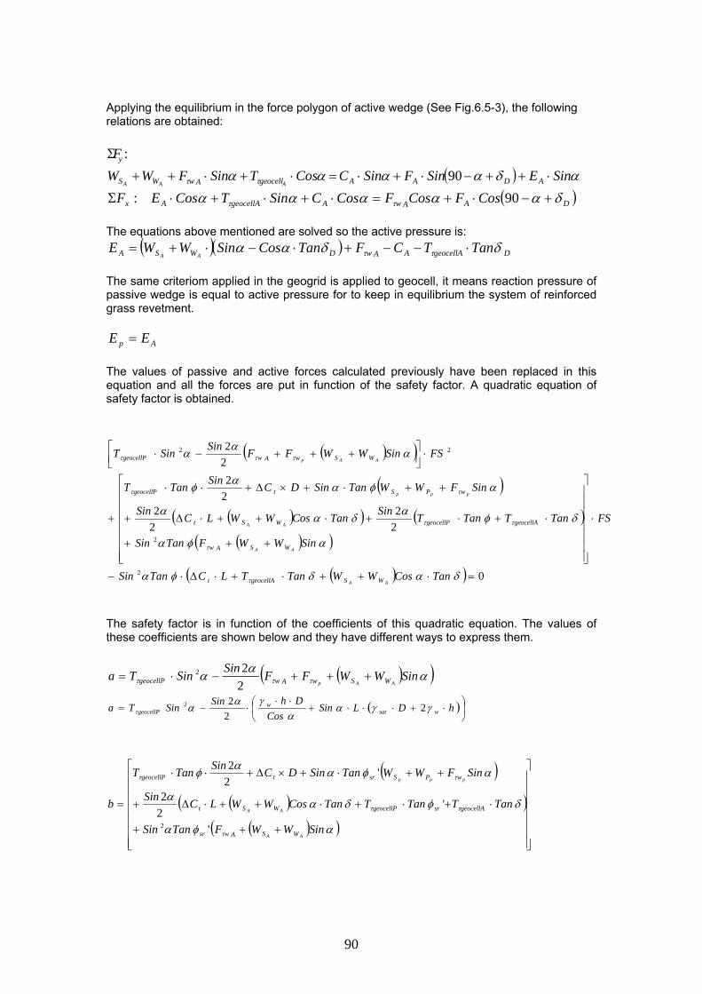
Applying the equilibrium in the force polygon of active wedge (See Fig.6.5-3), the following relations are obtained:

:yF Σ

( ) αδα ααα ττ SinES ADAAgeocellAwW AA⋅+SinFSinCCosTinFWWSA

+−⋅+⋅=⋅+⋅++ 90:xFΣ ( )DAAwAgeocellAA CosFCosFCosCSinTCosE δααααα ττ +−⋅+=⋅+⋅+⋅ 90

The equations above mentioned are solved so the active pressure is:

( )( )WSA WWEAA DgeocellAAAwD TanTCFTanCosSin δδαα ττ ⋅−−+⋅−⋅ +=

The same criteriom applied in the geogrid is applied to geocell, it means reaction pressure of

assive wedge is equal to active pressure for to keep in equilibrium the system of reinforced

he values of passive and active forces calculated previously have been replaced in this equation and all the forces are put in function of the safety factor. A quadratic equation of safety factor is obtained.

pgrass revetment.

Ap EE = T

( )( )

( )( )( ) ( )( )( )

( )( ) 02 =⋅++⋅+⋅Δ⋅−

⎥⎦⎢⎣δαδφα τ TanCosWWTanTLCTanSin

AA WSgeocellAt

22

22

22

22

2

22

⋅

⎥⎥⎥⎥⎥⎥⎤

⎢⎢⎢⎢⎢⎢⎡

+++

⋅+⋅+⋅++⋅Δ+

++⋅+×Δ+⋅⋅

+

⋅⎥⎦⎤

⎢⎣⎡ +++−⋅

αφα

δφαδαα

αφααφ

ααα

τ

ττ

ττ

τττ

FS

SinWWFTanSin

TanTTanTSinTanCosWWLCSin

SinFWWTanSinDCSinTanT

FSSinWWFFSinSinT

AA

AA

ppp

AAp

WSAw

geocellAgeocellPWSt

wPStgeocellP

WSwAwgeocellP

The safety factor is in function of the coefficients of this qua c equation. The values of these coefficients are shown below and they have different ways to express them.

drati

( )( )ααα τττ SinWWFFSinSinTAAp WSwAwgeocellP +++−⋅=

222 a

( )⎟⎠

⎞⎜⎝

⎛ ⋅+⋅⋅⋅+⋅⋅

⋅−= hDLSinCos

DhSinSinTa wsatw

geocellP γγαα

γαατ 2222

( )( )( )

( )( )⎥⎥⎥⎥⎥⎥⎥

⎦

⎤

⎢⎢⎢⎢⎢⎢⎢

⎣

⎡

+++

⋅+⋅+⋅++⋅Δ+

++⋅+×Δ+⋅⋅

=

αφα

δφδαα

αφααφ

τ

ττ

ττ

SinWWFTanSin

TanTTanTTanCosWWLCSin

SinFWWTanSinDCSinTanT

b

AA

AA

ppp

WSAwsr

geocellAsrgeocellPWSt

wPSsrtgeocellP

'

'22

'22

2

90

( )( )

( )( )( )( )

⎥⎥⎥⎥⎥⎥⎥

⎦

⎤

⎢⎢⎢⎢⎢⎢⎢

⎣

⎡

⋅+⋅⋅⋅⋅+

+⋅+⋅+⋅+Δ⋅+

+⋅⋅⋅+⋅××+×Δ+⋅⋅

=

DhLSinTan

TanTTanThDTanCosCLSin

SinhDDCos

TanDCSinTanT

b

satwsr

geocellAsrgeocellPwsatt

wsatsr

tsrgeocellP

γγαφ

δφγγδαα

αγγα

φαφ

ττ

τ

2'

'22

122

'22'

3

2

( )( )[ ]δαδφα τ TanCosWWTanTLCTanSincAA WSgeocellAtsr ⋅++⋅+⋅Δ⋅−= '2

( )⎥⎥⎦

⎤

⎢⎢⎣

⎡⎟⎟⎠

⎞⎜⎜⎝

⎛⎟⎟⎠

⎞⎜⎜⎝

⎛⋅+⋅+⋅⋅+Δ⋅⋅⋅−= αγγδφα τ CoshD

LT

TanCLTanSinc wsatgeocellA

tsr '2

2 0ax bx c+ + =

2 4

2b b acFS

a− ± −

=

If means that more cohesion in the reinforced grass revetment is needed so it is necessary to apply a pre-tension during the installation of the geocell.

1<FS

6.6. COHESION DUE TO GEOSYNTHETIC INTO THE SOIL-REINFORCED-GRASS

MATRIX OF THE REVETMENT Using the model of Jewell (1980) about the shear stress on reinforced soil we have that the cohesion in the soil due to geosynthetic is:

)'( srgicgeosynthet TanCosSinTC φθθ ⋅+⋅=Δ Details of parameters of this cohesion are well detailed in item 4.5. The tension is calculated using the criterion of Koerner in this thesis. The Koerner’s method is well explained in item 5.10 but in summarize it could be said that the tension of the geosynthetic is the difference between the active and passive pressure force of the grass revetment.

Ap ETE =+ ⇒ pA EET −= The tension in the geosynthetic is development when the safety factors of a grass revetment during an overtopping flow without geosynthetic lower than one 1<FS (review item 5.10). Replacing this value of the tension in the Jewell’s equation, the cohesion into the soil due to geogrid is defined like:

( ) )'(/ sr

pAgeocellgeogrid TanCosSin

AEEC φθθ ⋅+⋅

−=Δ

where is the area of the slope surface and the differences of active and passive wedge is: A

( ) ( ) ( )

( )( ) ( )( ) ⎥

⎦

⎤⎢⎣

⎡⎟⎠⎞

⎜⎝⎛ ⋅−+⋅⋅+⋅+

Δ+⋅

+⋅

−

⎥⎦⎤

⎢⎣⎡ ×Δ+−⋅⋅⋅+

−⋅⋅+⋅⋅=−

hSinhDSinTan

SinCC

CosDCos

LCCLhSinCos

SinhDLEE

wwsatsrroots

sr

sr

rootSwwsat

PA

γαγγαφ

αφαφ

αγδ

δαγγ

2122

''

'

91

7. CONCLUSION AND RECOMMENDATIONS

In general this thesis has analyzed the micro-stability and macro-stability of reinforced grass revetment located on inner slope during an overtopping event. The reinforcements analysed are geogrid and geocell. The general criterion used for both cases has been to keep the equilibrium between the forces that are acting on an individual soil particle at a micro level and in the layer of revetment at macro level. The models used from different authors to define the different forces that allow the particle stability or revetment stability have some limitations that make it necessary to insist and define the restrictions of micro and macro stability model proposed in this thesis. 7.1. ADITIONAL ROOT COHESION IN THE SOIL The method used to determine the cohesion into soil due to roots is the simple perpendicular root model (Wu et al, 1979, and O’Loughlin, 1982). This model is based on the concept that all roots break at the same time during the failure. Thus it tends to over-estimate up to 50% the root cohesion according some authors (Pollen and Simon, 2005). The method of progressive failure of the roots or fiber bundle model in root (Pollen and Simon, 2005) is a more realistic approximation since once a root is broken; the load is redistributed again on the rest of roots. The proposed equation in this thesis in respect to root cohesion that keep in equilibrium the system can be modified for this new model. One of the important parameters to determine root cohesion is root area ratio, or RAR. The information about what values are valid for Dutch dikes is scarce. The information analyzed in the MSc Thesis of Young (2005) suggests 0.25% for a depth between 15 and 40cm. This means one root of 3mm-diameter in a square of 50mm x 50mm or 400 roots/m2. These values look unrealistic. Information of Hanne from Msc thesis of Lavrina (2006) suggests 10% of 38 roots of the same diameter in the same square area or its equivalent 15000 roots/m2. These values look more realistic. This difference in the values influences substantially the results of root cohesion. An investigation to gather more information about RAR in Dutch sea dikes is required. This model assumes that the roots are perpendicular to failure plane initially. As the roots are pulled out, these make a distortion angle with the perpendicular axis to failure plane. In this thesis the failure plane is parallel to slope, thus the roots are assumed in perpendicular position to the slope. 7.2. ADITIONAL GEOCELL COHESION IN THE SOIL

The method used to determine the cohesion that the geosynthetics produce in the soil is described by Jewell’s model (1981). Information about tests to corroborate this model is scarce. Jewell’s model uses the same criterion of simple root perpendicular model to describe its theory, however here the geosynthetic is not necessarily in vertical position to failure plane like roots. In this thesis it is assumed that the failure plane is parallel to surface of dike so the geosynthetic would make an angle of 90 degrees with the perpendicular axis of failure plane. The distortion angle of geosynthetic would be defined by the deformation angle of geosynthetic that would have due to imperfections on the terrain or due to the tendency of water shear stress to deform the geosynthetic. This is feasible for geosynthetic like geogrid that its flexibility and low thickness helps its deformation making angles with the surface and the Jewell’s method could be applied. In case of geosynthetics like geoweb with higher thickness, these deformations are indistinguishable so Jewell’s method is doubtful application, or moreover it can not affirm or assume that the failure plane will be parallel to surface and it will be in the contact between geosynthetic and soil. For this reason and using the criterion of similar unit longitudinal deformation between soil and geosynthetic during an overtopping event, the following model has been development that defines the failure shear stress of grass revetment with geocell:

92

AATTanCosCos

AT

EE

c RRrs

sr

geocell

geo

geocell

soilf ⋅⋅+⋅⋅⎟

⎠⎞

⎜⎝⎛ +⋅⋅+= 2.145

2' '202 φη

φτ

It is obvious that the unit longitudinal deformations of soil and geocell are not necessarily similar so some tests are needed that show the veracity of this concept to validate this model. For this reason this hypothesis has not been used in the model of micro-stability and macro-stability of reinforced grass revetments. It is noted that as Jewell’s method as the proposed one in this thesis. A tension stress in the geosynthetic is necessary to produces cohesion in the soil. Therefore it is required that the geosynthetics need to be pre-tense when they are lied down on the slopes until to reach the stability of the system. The tension applied must be in the range to give enough cohesion to avoid erosion and to avoid the phenomenon of dilatation when the sand is dense. 7.3. ADITIONAL GEOSYNTHETIC COHESION IN UNSTABLE GRASS REVETMENTS

The additional soil cohesion into the soil of reinforced grass revetment due to geosynthetic, combining Jewell’s and Koerner’s method, is defined as:

( )⎟⎟⎠

⎞⎜⎜⎝

⎛⋅+⋅

−=Δ )'( sr

pAicgeosynthet TanCosSin

AEEC φθθ

( ) ( )

( ) ( )( )⎥⎥⎥⎥

⎦

⎤

⎢⎢⎢⎢

⎣

⎡

⎟⎟⎟⎟

⎠

⎞

⎜⎜⎜⎜

⎝

⎛

⋅−+⋅⋅⋅+⋅+⎟⎠⎞

⎜⎝⎛ ⋅⋅+

⋅+⋅

−

⎥⎦

⎤⎢⎣

⎡×⎟⎠⎞

⎜⎝⎛ ⋅⋅+−⋅⋅⋅+

−⋅⋅+⋅⋅=−

hSinhDSinTan

SinAATC

CosDCos

LAATCLhSin

CosSinhDLEE

wwsatsr

RRs

sr

sr

RRSw

wsatPA

γαγγαφ

αφαφ

αγδ

δαγγ

2122

'2.1

''

2.1

This equation is only valid for those grass revetments that during an overtopping event are unstable and the geosynthetics are used to stabilize them. The geosynthetics take the tension strengths produced by the differences of internal pressures between active wedge and passive wedge of grass revetments. 7.4. ADITIONAL COHESION IN STABLE GRASS REVETMENTS DUE TO TENSION

IN GEOGRID GENERATED DURING AN OVERTOPPING EVENT A stable grass revetment does not need to be reinforced with some geosynthetic. However, the grass revetment could be unstable during an overtopping event. For this reason it has been assumed that all tensional strength that is produced during an overtopping event is absorbed by geosynthetic like geogrid. The model has been made alike to a beam lied down on elastic foundation. The tensional strength that is generated in the soil due to moments are absorbed by geogrid. These moments appear since the shear stress exerted by fluid produce distortion angles in the geogrid. This geogrid has a tension that generates a cohesion expressed in the following equation:

)2

22

2(

ˆ3 '

20

20

srs

ogeogrid Tg

kM

Cosk

MSin

AeM

C φλπλπ

λ⋅⎟⎟⎠

⎞⎜⎜⎝

⎛ ⋅⋅−+⎟⎟

⎠

⎞⎜⎜⎝

⎛ ⋅⋅−⋅

⋅⋅⎥⎦

⎤⎢⎣⎡=Δ

There is not much information about the modulus of foundation per unit width . See item 5.3 and annex to review details of this equation. This value is important for calculating of additional cohesion in the soil due to geogrid during an overtopping event. It must be taken account the dilatation phenomenon.

( )k

93

7.5. MICRO-STABILITY METHOD In the model of micro-stability has been used in the equilibrium of vertical forces that are acting in the incipient movement of soil particles. These are lift forces, gravity forces and friction forces due to the cohesion that roots and geosynthetics exert on the soil. When the lift forces are lower than the added of all those mentioned above, the particles are in equilibrium. To define each force different theories have been used. They are: Lift forces defined by: Hoffman’s model (2006), that considers the intensity of turbulence, Carollo’s model (2005), that introduces the concentration factor, bent vegetation height and vegetation height in the calculation of depth average velocity. Friction forces due to cohesion stress, this is defined by friction angle and root and geosynthetic cohesion used in the macro-stabilization. Review item 7.2 Soil cohesion is a simple chemical effect and the theory of friction is not feasible. However, in this report it is assumed that friction theory is feasible. The friction coefficient is assumed equal to tangent of repose angle of the soil for definition. Using these criterions, the equilibrium of the particle would be defined by the following equation. See item 6.1.

( )

( ) ( )1

)2.1(21

61

82.9

'23

222222

321

≤+⋅⋅+⋅⋅+⋅⋅⋅⋅+⋅−⋅⋅⋅

⎟⎟⎠

⎞⎜⎜⎝

⎛⋅⎟

⎟⎠

⎞⎜⎜⎝

⎛ ⋅⋅⎟⎟

⎠

⎞⎜⎜⎝

⎛⋅⋅⋅⋅⋅

θφθπμρρπ

ν

SinTanCosA

TAATCdgd

hHhghI

hhMAghIdr

srgeoR

Rsws

a

s

v

a

w

sa

soo

In respect to the proposed model it is mentioned that: The lift forces are defined for a grass concentration lower than 50stems/dm2 and higher than 280stems/dm2. This means that the range between 50stem/dm2 and 280stem/dm2 are not considered in this model. Particle diameter: the representative diameter used in this model is not defined. Relative turbulence intensity: this factor needs to be defined in function of the relation between water height and vegetation height. It is assumed that smooth condition is when

the vegetation is submerged or 1≤hhs . Similarly root condition is when the vegetation is

not submerged or 1≥hhs .

Root and geosynthetic cohesion: Both cohesion forces are form a macro model and they are parallel to failure surface. These assumptions have been applied to micro level on a specific soil particle. The dilatation phenomenon of sands is not considered in this micro-stability model. From the model it could be concluded that a more tension in the geosynthetic more stability in the particle. This is not necessarily true since the rearrangement of dense sand would generate that particles climb up. Although there is not much information about the dilatation phenomenon of wet dense sands with a content of clays should be taken account. Friction forces: They are perpendicular to cohesive forces and they are generated when the particle tends to move up. It is has been assumed that friction coefficient is similar to tangent of repose angle of sand with a content of clays. This friction coefficient is a value that should be obtained from lab. Vertical stability: An analysis been made of vertical stability based on the principle that during turbulent flows the lift forces become the most important to cause erosion. Soil particle area under effects of forces: It has been approximated to a half area of a sphere.

94

7.6. MACRO-STABILITY METHOD

In the macro-stability of reinforced grass revetment, the equilibrium between the forces has been applied for active wedge and passive wedge. This is assuming that the failure plane is parallel to surface. The equality between pressure forces that exert each wedge is necessary to keep stable the system. The introduction of safety factor in the friction angle of root-soil, geosynthetic-root-soil and cohesion stress allows us to estimate if the system is stable or not and when it is safer. Equal to micro-stability, the cohesion stress are based on the following models: O’Loughlin, 1982, for root cohesion Jewell, 1980, y, for geosynthetic cohesion Koerner and Wu, 1991, for determine the tension stress in the geosynthetic Using those criterions, the macro-stability of a reinforced grass revetment with geogrid during an overtopping event is defined by the following equation. If the safety factor is higher than one for any tension so the system is stable.

( )

( )

( )( )

( )

( )( ) 0'

2

'22

12

2221

2

3

2

2

=⋅⋅⋅+⋅+Δ⋅⋅+

⋅

⎥⎥⎥⎥⎥⎥⎥

⎦

⎤

⎢⎢⎢⎢⎢⎢⎢

⎣

⎡

⋅⋅+⋅⋅⋅+

⋅⋅⋅+⋅+Δ⋅⋅+

⎟⎠

⎞⎜⎝

⎛+⋅⋅+

⋅⋅+×Δ

−

⋅⎥⎦

⎤⎢⎣

⎡⎟⎠⎞

⎜⎝⎛ ⋅+⋅⋅⋅+⋅⋅⋅

δαγγφα

γγφα

αδγγα

αγγ

αφ

γγαγα

TanCoshDCLTanSin

FS

hDLTanSin

CosTanhDCLSin

SinhD

CosTanDDC

FShDLSinDhSin

wsatt

wsat

wsatt

wsat

t

wsatw

Where:

( ) ⎟⎠⎞

⎜⎝⎛ ⋅+⋅+⎟

⎠⎞

⎜⎝⎛ ⋅⋅+=Δ )'(2.1 s

RRSt TanCosSin

AT

AATCC φθθ

( ) ⎟⎠⎞

⎜⎝⎛ ⋅+⋅+⎟

⎠

⎞⎜⎝

⎛ ⋅⋅+=Δ − )'(2.1' sR

RgSt TanCosSinAT

AA

TCC φθθ

Tension in this model is the tension stress that is applied in the geosynthetic during the installation. With this model, it can be calculated the tension needed in the grass revetment for a stable system and safety design. In the case of geocell, it is also used the same criterion of geogrid but no the criterion of item 7.2 to determine the cohesion. The stability depends on the tense strength in geocell how far to reach a safety factor higher than one. However, not only the tension strength in the geocell makes a stable system but also the shear strength between the contact of geocell walls and soil-root matrix helps. This means if the geocell is lied down on the slope without pre-tensed or tension is zero, the shear strength makes the system stable.

95

( )

( )( )

( )( )( )( )

( ) 0

222

1222

2

222

'2

3'

'

2'

,

22

=⎥⎥⎦

⎤

⎢⎢⎣

⎡⎟⎟⎠

⎞⎜⎜⎝

⎛⎟⎟⎠

⎞⎜⎜⎝

⎛⋅+⋅+⋅⋅+Δ⋅⋅⋅−

⋅

⎥⎥⎥⎥⎥⎥⎥

⎦

⎤

⎢⎢⎢⎢⎢⎢⎢

⎣

⎡

⋅+⋅⋅⋅⋅+

+⋅+⋅+⋅+Δ⋅+

+⋅⋅⋅+⋅××+×Δ+⋅⋅

+

⋅⎥⎦

⎤⎢⎣

⎡⎟⎠⎞

⎜⎝⎛ ⋅+⋅⋅⋅+

⋅⋅⋅−

αγγδφα

γγαφ

δφγγδαα

αγγαφαφ

γγαα

γαα

τ

ττ

τ

τ

CoshDL

TTanCLTanSin

FS

DhLSinTan

TanTTanThDTanCosCLSin

SinhDDCos

TanDCSinTanT

FShDLSinCos

DhSinSinT

wsatgeocellA

tsr

satwsr

geocellAsrgeocellPwsatt

wsatsr

tsrgeocellP

wsatw

geocellP

Where

( ) DCosSin

TanTanCoshDA

AT srwsat

cell

cellwallgeocellp

×⎟⎠⎞

⎜⎝⎛ +×⎟

⎟⎠

⎞⎜⎜⎝

⎛⋅⎟⎟⎠

⎞⎜⎜⎝

⎛−⋅⋅⋅+⋅= −

ααδ

φαγγτ

112

45'

2

( ) LTanTanCoshDA

AT srwsat

cell

cellwallgeocellA ×⎟

⎟⎠

⎞⎜⎜⎝

⎛⋅⎟⎟⎠

⎞⎜⎜⎝

⎛−⋅⋅⋅+⋅= − δφ

αγγτ 245

'2

If the tension force in geocell produced by the differences between pressures of active and passive wedge ( )pA EE − of reforced grass revetment is replaced in the above equation, it is obvious that the safety factor is higher than one. Therefore this tension does not need verification.

7.7. GENERAL RECOMMENDATIONS

In the set of equations development in this thesis are involved many parameters, they can be simplified if which are relevant or irrelevant are determined. The irrelevant parameters are those variables that not impact the results of the equation in big magnitude. The determination of importance of these factors is beyond the reach of this report and it is suggested to study in more detail. The parameters of easily tested for instance the tension roots and the parameters of difficult tested for instance the water shear stress should be also identified Eventhough it is ideal to make test in horizontal channels, from the equations described in the stability analysis is recommended the following: At micro-stability level for concentrations of stems higher than 280stems/dm2 (See table 3.5.3-1) the slope is not important, for this reason a horizontal channel or channel with slope can be described in the same way the phenomenon of incipient motion of soil particle. In the case of 50stems/dm2, the slope in the channel is important so in the laboratories is a factor that should be considered. At macro-stability level, the slope has influence in the stability of reinforced grass revetment in the proposed model so it is not the same to make test in horizontal channels that in channel with slope. It is recommended to make tests that describe the tension of geosynthetic compare with the cohesion produced in the layer of soil located over it to verify if the tension of geosynthetic produces shear stresses that get better the cohesion according the Jewell’s model based on Mohr’s equation and to related to dilatation phenomenon.

96

The forces which are present in the equilibrium of reinforced grass revetment at micro level and macro level can be defined by different authors taken account many parameters and limits. In this thesis is mentioned the models have been used to define each force however it is recommended to use other models to describe the same forces and to observe which is more adjustable to reality. For instance respect to water shear stress, it is used the average of this stress at macro-stability level, however this stress can be defined in function of relative turbulence intensity, concentration of grass and physical characteristics of vegetation and so on, theses factors have not been taken account in the model shown in this thesis. Other example it is the root cohesion and the simple root perpendicular model is used to estimate this cohesion, however there are more models that define the root cohesion. One of them is the progressive failure model; it can adjust the root cohesion more to reality. All this evaluation is beyond of this investigation. It should be taken account in the subsequent studies that the equations presented in this thesis are based on the theory of other pre-models so the mistakes that have the pre-models are introduced in these new equations for instance the additional cohesion produced by the root needs to be evaluated according the kind of vegetables that are on the slope.

97

REFERENCES ABE K., ZIEMER R., 1991, Effect of tree roots on a shear zone: modeling reinforced shear stress, Forestry and Forest Products Research Institute, Tsukuba, and USDA Pacific Southwest Research Station, Forest Service, Arcata. Japan, USA. BRANSBY M.F., DAVIES M.C.R., MICKOVSKI S.B., SONNENBERG R., BENGOUGH A.G & HALLET P.D., 2006, Stabilization of slopes by vegetation reinforcement, University of Dundee & Scottish Crop Research Institute, UK. CAROLLO F.G., FERRO V., TERMINI D., 2005, Flow Resistance law in Channels with Flexible Submerged Vegetation, Journal of Hydraulic Engineering, Vol.131, No 7, July 1, 2005, ASCE, University of Palermo, Italy. CHENG H., YANG X., LIU A., FU H, WAN M, 2002, A study on the performance and mechanism of Soil-Reinforcement by herb root system, Nanchang Water Conservancy and Hydropower College and Jiangxi Provincial Highway Administrative Bureau, China DARTEVELLE, S., 2003, Numerical and granulometric approaches to geophysical granular flows, Ph.D. thesis, Michigan Technological University, Department of Geological and Mining Engineering, Houghton, Michigan, USA. FISCHENICH, C., 2001, Stability thresholds for streams restoration materials, USAE Research and Development Center, Environmental Laboratory, 3909 Halls Ferry Rd., Vicksburg, MS 39180. FORD A., 2003, A comparison of Pampas Grass (Cortaderia jubata), Coyote Bush (Bacharis pillularis), and Poison Oak (Toxicondendron diversilobum) on Soil Cohesion in Big Sur, California, Berkeley, University of California, USA HETÉNYI M., 1993, Beams on elastic foundation, Scientific Series, Volume XVI, University of Michigan, USA HEWLETT H W M, BOORMAN L A, BRAMLEY M E, 1987, Design of reinforced grass water ways, CIRIA Report 116, ISBN 0 86017 285 6, London. HOFFMANS G., 2006, Stability of Stones under Non-Uniform flow,Ministry of Transpor, Public Works and Water management, DWW-2006-085, ISBN-10 90-369-5619-6, Netherlands. HR WALLLINGFORD LTD, 1999, Wave overtopping of Seawalls, Design and Assessment Manual, R&D Technical Report W178, Oxfordshire. KOERNER R., HWU B.-L., 1991, Stability and Tension Considerations regarding cover soils in geomembrane lined slopes, Jour. of geotextiles and geomembranes, 1991, Vol. 10, No.4, pp.335-355, Pensilvania, USA. KOERNER R., 2005, Designing with Geosynthetics, Pearson Prentice Hall, ISBN 0-13-145415-3, New Jersey, USA. MADHAV M.R., GURUNG N. and IWAO Y., 1998, A theoretical model for the pull-out response of geosynthetic reinforcement, Geosynthetics International, 1998, Vol5, No 4. MAASKANT I., 2005, Toepassingsmogelijkheden van vetiver gras en Cyperus rotundus op dijken, Msc. Thesis, Delft University of Technology, Delft, Netherlands MUIJS J.A., 1999, Grass cover as a dike revetments (translation of TAW-brochure “Grasmat als Dijkbekleding” 9 febraury 1999, TAW: Technical Advisory Committee for Flood Defence, The Netherlands. O’LOUGHLIN C., ZIEMER R., 1982, The importance of root strength and deterioration rates upon edaphic stability in steepland forest, I.U.F.R.O. Workshop P.1.07-00 Ecology of Subalpine Ecosystems as a Key to Management. 2-3 August 1982, Corvallis, Oregon. Oregon State University, Corvallis, Oregon, USA PILARCZYK K, 2000, Geosynthetics and Geosystems in Hydraulic and Coastal Engineering, Rijkswaterstaat, A.A.Balkema/Rotterdam/Brookfield, ISBN 90 5809 302 6, Delft, Netherlands.

98

POLLEN N., SIMON A., 2005, Estimating the mechanical effects of riparian vegetation on stream bank stability using a fiber bundle model, Channel and Watershed Processes Research Unit, National Sedimentation Laboratory, ARS, USDA, Oxford, Mississippi, USA POLLEN N., 2006, Temporal and spatial variability in the Root-Reinforcement of Streambanks: Accounting for soil shear strength and moisture, United States Department of Agriculture, Agriculture Research Service, USA. RIMOLDI P., RICCIUTI A., RECALCATI P., Steep reinforced slopes, Geosynthetics Division S.D.RAJAN, 2000, Introduction to structural analysis design, Deparment of Civil and Environmental Engineering, Arizona State University, ISBN 0-471-31997-X, USA SCHÜTTRUMPF H, 2003, Wave overtopping flow on seadikes – Experimental and Theoretical Investigations. PIANC Bullentin 149. SHEN H.W., 1973, Flow resistance over short simulated vegetation and various tall simulated vegetation grouping on flow resistance and sediment yield, Environmental Impact on Rivers, Rivers Mechanics III, Fort Collins, Colo SPRANGERS H, 1999, Vegetation dynamics and erosion resistance of sea dyke grassland. Deparment of Environmental Sciences, Section Nature conservation and Plant ecology, Wageningen Algricultural University, Wageningen, The Netherlands. SMITH G.N., 1983, Element of Soil Mechaniccs for Civil and Mining Engineers, Heriot-Watt University, Edinburgh, Granada publishing, ISBN 0-246-11765-6, Great Britain VAN DE MEER J W, 2002, Technical Report: Wave Run-up and Wave Overtopping at Dikes, TAW: Technical Advisory Committee for Flood Defence, The Netherlands. VAN DEN BOS W., 2006, Erosiebestendigheid van grasbekleding tijdens golfoverslag, MSc Thesis, Delft University of Technology, Netherlands VAN GERVEN K.A.J., VAN DER MEER J.W., VAN HEEREVELD M.A., AKKERMAN G.J., 2005, ComCoast WP3 Development of alternative overtopping-resistant Sea Defences. Phase 2: Elaboration of smart grass reinforcement concept. Royal Haskoning and Infram, Project number 9P8624.C0, Netherlands. VAVRINA, L, 2006, Erosion Processes on Dike Slopes, MSc. Thesis, University of Duisburg-Essen and TUDelft. VERHAGEN H.J., 2000, Grass cover on dikes and slope protections, UNESCO-IHE, Delft. VERHEIJ H.J., KRUSE G.A.M., NIEMEIJER J.H., SPRANGERS J.T.C.M., DE SMIDT J.T. AND WONDERGEM P.J.M., 1997, Technical report: Erosion resistance of grassland as dike covering, TAW: Technical Advisory Committee for Flood Defence, The Netherlands. WHITEHEAD D.C., 2000, Nutrient elements in grassland, soil-plant-animal Relationships, Deparment of Soil Science, University of Reading UK, ISBN 0-85199-437-7, CABI Publishing, London, UK. WIND H. G., 1987. Impact of Sea Level Rise on Society, University of Twente, Enschede & Delft Hydraulics, Report of a project-planning session/Delft 27-29 August 1986, A.A.Balkema/Rotterdam/Brookfield. TAW, 1997, Technical report: Erosion resistance of grassland as dike covering, YOUNG M.J., 2005, Wave overtopping and grass cover layer failure on the inner slope of dikes, MSc Thesis WSE-CEPD-05-03, UNESCO-IHE, Delft.

99

APENDIX I: CALCULATION MODEL OF WAVE OVERTOPPING DESIGN DISCHARGE VAN DE MEER’S MODEL

This model predicts discharge calculating the average overtopping rates for single peaked wave spectra. This means the distribution of wave overtopping volumes can be calculated for each wave. The disadvantage is that the overtopping discharge does not take into account the hydraulic characteristics of the flow which it generates or geotechnical properties of soil where it pass over. The overtopping discharge is different for breaking waves and non-breaking waves. The method is well-explained at Technical Report Wave Run-up and Wave Overtopping at Dikes as well as different values and parameters used. Only general statements are mentioned in this item. The wave overtopping formulae are exponential function and have this form: For breaking waves )2( <≈obεγ :

⎟⎟⎠

⎞⎜⎜⎝

⎛−<⎟

⎟⎠

⎞⎜⎜⎝

⎛−=

ββ γγγγγγξξγ

α fmo

c

vfbom

cob

mHR

HR

gHq 13.2exp2.013.4exp

tan067.0

03

0

For non-breaking waves )2( >≈obεγ : :

⎟⎟⎠

⎞⎜⎜⎝

⎛−=

βγγ fm

c

mHR

gHq 13.2exp2.0

03

0

Where : average wave overtopping discharge [m3/s per m] q g : acceleration due to gravity [m/s2]

: significant wave height at toe of dike [m] 0mH

oξ : breaker parameter o

o sTanαξ =

os : wave steepness 210

02

−

=m

mo gT

Hs

π

: spectral wave period at toe of dike 10−mT αTan : angle of outer slope. For differents slopes can be calculated as:

BLZH

Tanslope

m

−+

= %205.1α

: free crest height above still water line cR bγ : Influence factor for a berm

fγ : influence factor for roughness elements on slope. 0.1=fγ Grass

βγ : influence factor for angled wave attack

Vγ : influence factor for vertical wall on slope The used parameters in the formulae are in detail at Technical Report Wave Run-up and Wave Overtopping at Dikes (TAW, 2002)

100

SCHÜTTRUMPF’S MODEL

This method is based on two dimensional equation motion (Navier-Stokes equations) and take into account the interaction between the soil properties and overtopping flow. For this reason it concentrates on the calculation of velocities and layer thicknesses, which are a good prediction of erosion and infiltration into the clay coverage of sea dikes. The formulas calculate the overtopping velocities and layer thicknesses from outer slope and crest to inner slope. The flow is described from the generation on the outer slope after wave breaking. Overtopping velocity helps to get a better understanding about erosion as well as the overtopping layer thicknesses helps infiltration. The overtopping velocities are higher with shorter thicknesses and there is much erosion when the slopes are steeper. The infiltration is higher when the slopes are flatter and the erosion decreases. The overtopping flow velocities are not constant in either the outer slope, crest or inner slope. The report Overtopping Flow Parameters on the inner slope of Seadikes (H.Schüttrumpf, H.Oumeraci) explains this model in detail. In this item only the formulas relating to sections on the crest and at inner slope will be shown because they are related. The formulas which describe the layer thicknesses and velocity overtopping over sea dike is shown in the following:

• Layer thickness on the crest (c) of the dike:

( ) ( ) ⎟⎠⎞

⎜⎝⎛−==

Bx

cxhxh ccccc 3exp0

: Layer thickness at ch cx

cx : coordinate along the dike crest

B : Width of the dike crest : dimensionless coefficient 3c

• Overtopping flow velocity on the dike crest: it is influenced by surface friction and the crest width.

⎟⎟⎠

⎞⎜⎜⎝

⎛ ⋅−==

c

ccccc h

xfxVxV

2exp)0()(

Where: : Overtopping velocity on the dike crest at distance ( cc xV ))

cx : Overtopping velocity at the beginning of the dike crest ( 0=cc xV : Friction coefficient. f 02.0=f for smooth slopes . This coefficient is determined experimentally.

• Layer thickness on the inner slope of the dike:

( )B

BB V

hVh 00

= Layer thickness along the inner slope at distance Bs

Where: ( )00 == BB shh Layer thickness at 0=Bs

( ) ( )BxVV ccB ==0 Overtopping velocity at the end of the dike crest

• Overtopping flow velocity on the inner slope:

101

( )( )

( )⎟⎠⎞

⎜⎝⎛+

⎟⎠⎞

⎜⎝⎛+

=

201

20

1

1

11

tkTanhkh

fV

tkTanhfhkV

sV

B

B

BB

BB

Where: V Overtopping velocity on the inner slope at distance ( )BB s Bs

Bs Coordinate along the inner slope

( )

βββ sin2

sinsin0

22

2

gs

gV

gVt BBB ++−≈

Bh

fgk βsin21 =

mTan :1=β β is angle of inner slope

FIG.3.2: Definition sketch for overtopping flow parameters on the outer slope, dike crest and inner slope (Source: H.Schüttrumpf, 2001, Wave Overtopping flow on seadikes)

BESLEY’S MODEL

This model is commonly used in the coastline of UK. It is based upon model tests which intend to represent the discharges in different section types of dikes. Therefore, they have an error margin when they are applied to the profile of dike and condition non-similar to original. Continuous and splash overtopping discharges have been considered in these tests. The wave overtopping discharge is calculated for a determined return period of waves and water level. This return period depends on the lifetime of structure, maximum water level, maximum wave and the use of the structure so public opinion is involved in this calculation. This method is based on Owen formula (1980) who proposed an overtopping discharge for each typical structure. It this item only models of overtopping discharges for smooth impermeable slope and rough and armoured slopes will be described. More detail of this method is described in Wave Overtopping of Seawalls Design and Assessment Manual (HR Wallingford, 1999) in which each section type of dike has its own model of wave overtopping. The mean overtopping discharge over different sea dikes with smooth impermeable slopes

and rough and armoured slopes are defined below. )1( =r

102

sm gHTQQ =* Valid for 30.005.0 * << R

( ) 5.0*sm

c

gHTR

R =

( )rBRAQ /exp ** −= Where: : mean overtopping discharge rate per meter run of seadike Q : Wave period at the toe of the dike mT g : Acceleration due to gravity

: Significant wave height at the toe of the dike sH

cR : Freeboard of the seadike (the height of the crest of the wall above still water level)

A and B : empirically coefficients which depend on the profile of the seadike. Outer slope use 4:1 216.1 −= EA and 0.41=B

:r Typical roughness coefficients. Seadike with smooth impermeable slopes . Turf slope )1( =r )0.19.0( −=r

:rO ratio of discharge under angled wave attack to that under normal attack

, 2000152.01 β−=rO β is the angle of wave attack to the normal, in

degrees 00 600 ≤< β The used parameters in the formulae are in detail at Wave Overtopping of Seawalls Design and Assessment Manual (HR Wallingford, 1999).

103

APENDIX II: TENSILE STRENGTH OF DIFERENT PLANTS

Source: Cheng H, Yang X, Liu A, Fu H, Wan M , 2002, A study of performance and mechanism of soil-reinforcement by Herb root system Vetiver grass (vetiveria zizanioides)

Bermuda grass (Cynodon dnactylo) and Manila grass (zoysia matrella merr)

White clover (trifolium repens) and Bahia grass (paspalum notatum flugge)

104

Late Juncellus (Juncelles serotinus) Dallis grass (paspalum dilatatum poir)

Centipedegrass (Ere mochioa ophiurides hack)

105

APENDIX III: COEFFICIENT ACCORDING USDA VALUES OF GRASS ROUGHNESS COEFFICIENT nC

Grass Roughness Coefficient, Cn

Stem Height (m) Excellent Very Good Good Fair Poor

0.075 0.168 0.157 0.142 0.122 0.111 0.150 0.243 0.227 0.205 0.177 0.159 0.225 0.301 0.281 0.254 0.219 0.197

Source: .

VALUES OF COVER FACTOR fCCover Factor, Cf Growth Form Excellent Very Good Good Fair Poor

Sod 0.98 0.95 0.90 0.84 0.75 Bunch 0.55 0.53 0.50 0.47 0.41 Mixed 0.82 0.79 0.75 0.70 0.62

COEFFICIENTS FOR PERMISSIBLE SOIL SHEAR STRESS (USDA, 1987)

ASTM Soil Clasification Description

Range of plasticity

index 1c 2c 3c 4c 5c 6c (SI)

10≤PI≤20 1.07 14.3 47.7 1.42 -0.61 4.8x10-3

GM Silty gravels, gravel-sand silt mixtures 20≤PI - - 0.076 1.42 -0.61 48

10≤PI≤20 0.0477 2.86 42.9 1.42 -0.61 4.8x10-2

GC Clayey gravels, gravel-sand-clay mixtures 20≤PI - - 0.119 1.42 -0.61 48

10≤PI≤20 1.07 7.15 11.9 1.42 -0.61 4.8x10-3

SM Silty sands, sand-silt mixtures 20≤PI - - 0.058 1.42 -0.61 48

10≤PI≤20 1.07 14.3 47.7 1.42 -0.61 4.8x10-3

SC Clayey sands, sand-clay mixtures 20≤PI - - 0.076 1.42 -0.61 48

10≤PI≤20 1.07 7.15 11.9 1.48 -0.57 4.8x10-3

ML Inorganic silts, very fine sands, rock flour, silty or

clayey fine sands 20≤PI - - 0.058 1.48 -0.57 48

10≤PI≤20 1.07 14.3 47.7 1.48 -0.57 4.8x10-3

CL

Inorganic clays of low to medium plasticity,

gravelly clays, sandy clays, silty clays, lean

clays

20≤PI - - 0.076 1.48 -0.57 48

10≤PI≤20 0.0477 1.43 10.7 1.38 -0.373 4.8x10-2

MH

Inorganic silts, micaceous or

diatomaceous fine sands or silts, elastic silts

20≤PI - - 0.058 1.38 -0.373 48

CH Inorganic clays of high plasticity, fat clays 20≤PI - - 0.097 1.38 -0.373 48

106