Regulated Price Plan Manual - OEB
45
Regulated Price Plan Manual Ontario Energy Board Issued October 13, 2020 (Replacing version issued on February 16, 2016)
Transcript of Regulated Price Plan Manual - OEB

Regulated Price Plan
Manual
Ontario Energy Board
Issued October 13, 2020
(Replacing version issued on February 16, 2016)

NOTE TO READERS: On October 13, 2020 the following revisions were made to the Manual: (a) revisions to reflect the repeal, in 2017, of subsection 79.16(3) of the Ontario Energy
Board Act, 1998, which required the OEB, when setting Regulated Price Plan prices, to “take into account balances in variance accounts established under section 25.33 of the Electricity Act, 1998 and make adjustments with a view to eliminating those balances within 12 months or such shorter time periods as the Minister may direct”; the Manual now provides that although 12 months is the default period for eliminating variances, the Ontario Energy Board may in special circumstances choose a longer period of time;
(b) the Manual now specifies to a second decimal place (0.85) the target ratio between the upper and lower tier prices; and
(c) minor housekeeping edits to reflect: (i) the cessation of the Debt Retirement Charge; (ii) other changes in regulation; and (iii) changes to O. Reg. 95/05 (Classes of Consumers and Determination of Rates) and the Standard Supply Service Code that, as of November 1, 2020, allow Regulated Price Plan consumers who would otherwise be charged on the basis of time-of-use prices to elect instead to be charged on the basis of tiered prices.

RPP Manual – October 13, 2020 Page i
TABLE OF CONTENTS 1. INTRODUCTION .......................................................................................................................... 1
About this Manual ................................................................................................................................ 1 Purpose ................................................................................................................................................. 2 Authority for the OEB to Set RPP Prices ............................................................................................. 3 Total Prices Paid by Consumers ........................................................................................................... 3 Process for RPP Price Determinations ................................................................................................. 5 Using this Manual ................................................................................................................................ 5 Roles of Participants ............................................................................................................................. 6 Prices..................................................................................................................................................... 7 Definitions ............................................................................................................................................ 7
2. METHODOLOGY FOR CALCULATING THE RPP SUPPLY COST............................................... 9 Introduction .......................................................................................................................................... 9 Overview of the Ontario Electricity Market Structure ........................................................................ 9 Overall Methodology for Forecasting the RPP Supply Cost ................................................................ 9 Computation of the RPP Supply Cost .................................................................................................12
3. METHODOLOGY AND TIMING FOR SETTING RPP PRICES .................................................. 18 Introduction .........................................................................................................................................18 Timing for RPP Price Setting ..............................................................................................................18 Setting the Price Component to True-Up RPP Supply Cost Variance ...............................................19 Setting the Average RPP Price ............................................................................................................20 Setting the Tiered Prices ......................................................................................................................21 Setting the Time-of-Use Prices ............................................................................................................22 Price True-Ups for Extraordinary Circumstances ..............................................................................29
4. METHODOLOGY AND TIMING FOR VARIANCE TRACKING ................................................. 31 Introduction .........................................................................................................................................31 Monthly Variances ..............................................................................................................................31 Variance Forecasting ............................................................................................................................33 Variance Monitoring ...........................................................................................................................34 Frequency of Variance Monitoring ......................................................................................................34
5. TIMING FOR RPP PRICE ADJUSTMENTS OR PRICE STRUCTURE CHANGES ....................... 36 Introduction .........................................................................................................................................36 Timing of Notification of Price or Price Structure Change .................................................................36 Timing of Implementation by Distributors .........................................................................................37
6. METHODOLOGY FOR DETERMINING FINAL RPP VARIANCE SETTLEMENT AMOUNTS ... 38 Introduction .........................................................................................................................................38 Determination of Final RPP Variance Settlement Amount and Rate .................................................39
APPENDIX A: TRUE-UP EQUATIONS .......................................................................................... 41

RPP Manual – October 13, 2020 Page ii
LIST OF FIGURES
FIGURE 1: RETAIL ELECTRICITY PRICE UNDER THE REGULATED PRICE PLAN ............................................. 4 FIGURE 2: PROCESS FOR RPP PRICE............................................................................................................... 5
RPP Manual – October 13, 2020 Page 1
1. INTRODUCTION
About this Manual Under amendments to the Ontario Energy Board Act, 1998 (the Act) contained in the Electricity Restructuring Act, 2004, the Ontario Energy Board (the OEB) is mandated to develop a regulated price plan (the RPP). The RPP replaced the electricity commodity pricing regime that went into effect on April 1, 2004, and took effect on April 1, 2005 for eligible consumers.1 This Regulated Price Plan (RPP) Manual (the Manual) was initially prepared by the OEB within the context of a larger regulatory proceeding (designated as RP-2004-0205) in which interested parties assisted the OEB in developing the elements of the RPP. This Manual describes the processes and methodologies that the OEB uses to support its responsibilities with respect to setting prices under the RPP. The Manual is updated from time to time to reflect changes to those processes and methodologies and other relevant developments. Implementation of the RPP by licensed distributors is addressed primarily in the OEB’s Standard Supply Service Code. The Standard Supply Service Code also contemplates that various elements of the RPP, including prices, will be determined in accordance with this Manual. Related documents and OEB decisions that describe processes and actions that other parties use to fulfill their responsibilities under or in relation to the RPP include:
Ontario Energy Board Instruments Retail Settlement Code (the RSC); Standard Supply Service Code (the SSS Code); Rate Orders; and Licences.
Independent Electricity System Operator (the IESO) Instruments Ontario Market Rules.
1 Consumers eligible for the RPP are identified in O. Reg. 95/05 (Classes of Consumers and Determination of Rates) (the RPP Regulation).

RPP Manual – October 13, 2020 Page 2
Three other documents relate to the process for setting the RPP price, as described in this Manual: Ontario Wholesale Electricity Market Price Forecast, which contains the market
price forecast used in the RPP price setting process. Regulated Price Plan Price Report, which describes the data sources for the
forecasts and the application of the methodology in this Manual to arrive at the prices for the RPP.
The RPP Regulation, which sets out who is eligible for the RPP and prescribes rules regarding the manner in which the OEB determines rates for purposes of the RPP.
This Manual consists of six chapters as follows: Chapter 1. Introduction Chapter 2. Methodology for Calculating the RPP Supply Cost Chapter 3. Methodology and Timing for Setting RPP Prices Chapter 4. Methodology and Timing for Variance Tracking Chapter 5. Timing for RPP Price Adjustments or Price Structure Changes Chapter 6. Methodology for Determining Final RPP Variance Settlement
Amounts
Purpose The purpose of this Manual is to define and explain the methodologies and internal processes that the OEB uses in determining electricity commodity prices that are charged to RPP consumers. This Manual includes processes for calculating and setting the RPP prices, including separate prices for consumers with eligible time-of-use (or smart) meters that are charged on the basis of a time-of-use pricing structure and for consumers that are charged on the basis of a tiered pricing structure (including consumers with conventional meters and consumers with eligible time-of-use meters that opt out of time-of-use pricing in accordance with the Standard Supply Service Code); for monitoring and truing up variances between the forecast RPP price and the actual cost of RPP supply; for resetting the RPP price; and for calculating the final RPP variance settlement amount for consumers leaving the RPP. In keeping with legislation, the RPP prices set by the OEB are intended to reflect the cost of supply over time.
RPP Manual – October 13, 2020 Page 3
Authority for the OEB to Set RPP Prices Section 79.16 of the Act assigns the OEB responsibility for determining electricity commodity prices for eligible consumers. Consumer eligibility for RPP prices is determined by the RPP Regulation. The RPP Regulation requires the OEB to forecast the cost of electricity used by these consumers and to ensure that the prices reflect that cost2. As required by the RPP Regulation, the initial RPP commodity prices determined by the OEB under both the tiered structure and the time-of-use structure were set to remain in effect for a period of at least 12 months. Subsequently, the OEB has reviewed and, where required, changed the RPP commodity prices every six months as discussed in Chapter 3.
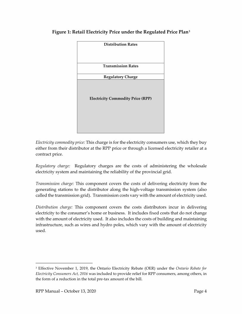
Total Prices Paid by Consumers The electricity commodity prices under the RPP comprise only one element of the total price paid by consumers taking RPP supply. Figure 1 shows the other elements that comprise the final retail consumer bill. The height of the bars in the diagram is roughly proportional to each element’s relative share of the total retail electricity bill. There is also a brief description of each component of the consumer bill following the diagram.
2 The Act formerly required the OEB, when setting RPP prices, to “take into account balances in variance accounts established under section 25.33 of the Electricity Act, 1998 and make adjustments with a view to eliminating those balances within 12 months or such shorter time periods as the Minister may direct”, but that provision was repealed in 2017.
RPP Manual – October 13, 2020 Page 4
Figure 1: Retail Electricity Price under the Regulated Price Plan3
Distribution Rates
Transmission Rates
Regulatory Charge
Electricity Commodity Price (RPP)
Electricity commodity price: This charge is for the electricity consumers use, which they buy either from their distributor at the RPP price or through a licensed electricity retailer at a contract price. Regulatory charge: Regulatory charges are the costs of administering the wholesale electricity system and maintaining the reliability of the provincial grid. Transmission charge: This component covers the costs of delivering electricity from the generating stations to the distributor along the high-voltage transmission system (also called the transmission grid). Transmission costs vary with the amount of electricity used. Distribution charge: This component covers the costs distributors incur in delivering electricity to the consumer’s home or business. It includes fixed costs that do not change with the amount of electricity used. It also includes the costs of building and maintaining infrastructure, such as wires and hydro poles, which vary with the amount of electricity used.
3 Effective November 1, 2019, the Ontario Electricity Rebate (OER) under the Ontario Rebate for Electricity Consumers Act, 2016 was included to provide relief for RPP consumers, among others, in the form of a reduction in the total pre-tax amount of the bill.

RPP Manual – October 13, 2020 Page 5
Process for RPP Price Determinations Figure 2 below illustrates the process for setting RPP prices and the decisions to be made in that process. The RPP supply cost and the accumulated variance between actual and forecast costs (carried by the IESO) both contribute to the base RPP price, which is set to recover the full costs of supply. The remainder of the process is also based on forecasts of prices and of consumption patterns. For consumers with eligible time-of-use meters that are being charged on the basis of time-of-use prices, the next step is to analyze the pattern of prices in order to determine what the pattern of prices should be, both in terms of the three price levels (on-peak, mid-peak and off-peak) and in terms of the daily times of application of these prices. These differ seasonally. For consumers that are not being charged on the basis of time-of-use prices, the next step is to analyze the tier structure of their prices. From the tier structure is derived the RPP prices that such consumers will pay.
Figure 2: Process for RPP Price
This Manual is organized according to this basic process. Chapter 2 describes the computation of the RPP supply cost. Chapter 3 explains the methodology used for setting RPP prices. Chapter 4 describes tracking and monitoring the IESO’s variance account. Chapter 5 deals with the timing of price adjustments and price structure changes. Chapter 6 describes the methodology to be used for determining the final RPP variance settlement amounts for consumers that leave the RPP. Appendix A describes the equations used to determine the cost variance component of the process shown in Figure 2.
Using this Manual The processes and methodologies in this Manual relate to activities of the OEB and, for one particular function, to distributors with final RPP variance settlement responsibilities for RPP consumers. The OEB uses these methodologies and processes to assist in determining electricity commodity prices for the RPP and to support the calculation of final RPP variance settlement amounts for consumers leaving the RPP. This Manual also serves as a guide to interested parties in understanding how the OEB determines prices for the Regulated Price Plan.
RPP Manual – October 13, 2020 Page 6
Roles of Participants This Manual describes the roles of various participants in or related to the RPP process, but does not directly place obligations on them. However, other instruments (such as the SSS Code) refer to this Manual with respect to some obligations, particularly the determination of the final RPP variance settlement amount for consumers leaving RPP supply. Requirements placed directly on participants are contained in legislation, regulations, licences, codes and the Market Rules, as applicable. The majority of RPP requirements and obligations for electricity distributors are set out in the SSS Code. Roles of electricity distributors Distributors are the point of contact, both physical and financial, for most consumers in Ontario’s electricity system. They provide distribution service which allows electricity to be delivered to the place of consumption. Under section 29 of the Electricity Act, 1998 (the “Electricity Act”), a distributor is also required to sell electricity to every person connected to the distributor's system, except those consumers that opt to purchase electricity from a competitive retailer. Other roles include:
Meter reading; Billing; Electricity supplier for consumers taking RPP supply; and Electricity supplier for consumers not eligible for RPP supply and not taking
supply from a competitive retailer. Roles of the Independent Electricity System Operator (IESO) The IESO’s main roles are to plan the electricity system, procure resources, administer the wholesale electricity market in Ontario and to direct the operation of the IESO-controlled grid, scheduling and dispatching the electricity system to maintain safe and reliable electricity supply. The IESO settles the wholesale market with all wholesale market participants, both buyers and sellers. The other main responsibilities of the IESO are forecasting electricity demand and supply adequacy and contracting for supply or demand management. The IESO roles with respect to the RPP are:
to include the global adjustment in its monthly settlements;4
to hold in a variance account the amounts due to differences between actual electricity commodity prices and the forecast-based RPP prices; and
4 The global adjustment was formerly also referred to as the “Provincial Benefit”.
RPP Manual – October 13, 2020 Page 7
to provide the OEB with information as may be required by the OEB for purposes of the determination of RPP prices and the final RPP variance settlement amount.5
Roles of Ontario Electricity Financial Corporation (OEFC) The Ontario Electricity Financial Corporation (“OEFC”) is responsible for holding and defeasing that part of the former Ontario Hydro’s debt that was not assigned to the successor operating companies. In conjunction with that responsibility, OEFC became the counterparty to the non-utility generator (NUG) contracts signed by the former Ontario Hydro. As such, it is the metered market participant for the NUGs.6 OEFC’s role with respect to the RPP is to provide the OEB with information as may be required by the OEB for purposes of the determination of RPP prices.
Prices This Manual describes the methodology that the OEB uses to determine commodity prices for RPP consumers, but does not contain the prices themselves. RPP prices, as determined from time to time, are posted on the OEB’s website.
Definitions The following defined terms are used in this Manual.
“Act” means the Ontario Energy Board Act, 1998, S.O. 1998, c. 15, Schedule B;
“OEB” means the Ontario Energy Board; “consumer credit balance” means a balance in the variance account carried by the IESO for RPP consumers that will be credited to RPP consumers; “consumer debit balance” means a balance in the variance account carried by the IESO for RPP consumers that is owed to the IESO by RPP consumers;
“conventional meter” means a meter other than an eligible time-of-use meter;
5 Among others, section 23 of the Electricity Act states that “The IESO shall provide the OEB, the IESO and the Market Surveillance Panel with such information as the OEB, IESO or Panel may require from time to time”. 6 OEFC is also the counterparty to contracts in relation to two additional generation facilities in respect of which contingency support payments to Ontario Power Generation (OPG) are made through the global adjustment. See O. Reg. 427/04 (Payments to the Financial Corporation re Section 78.2 of the Act) made under the Act, as amended effective January 1, 2009.
RPP Manual – October 13, 2020 Page 8
“Electricity Act” means the Electricity Act, 1998, S.O. 1998, c. 15, Schedule A;
“eligible time-of-use meter” means an interval meter or a meter that measures and records electricity use during each of the periods of the day referred to in section 3.4.1 of the SSS Code cumulatively over a meter reading period; “final RPP variance settlement amount” means the amount charged or credited to an RPP consumer in accordance with section 3.7 of the SSS Code;
“global adjustment” or “GA” means the adjustment referred to in section 25.33 of the Electricity Act and made in accordance with regulations made under that section;
“IESO” means the Independent Electricity System Operator; "Market Rules" means the rules made under section 32 of the Electricity Act;
“non-RPP consumer” means a consumer that is not an RPP consumer;
“Retail Settlement Code” or “RSC” means the code issued by the OEB which, among other things, establishes a distributor’s obligations and responsibilities associated with financial settlement among retailers and customers and provides for tracking and facilitating customer transfers among competitive retailers; “RPP consumer” means a consumer that pays the commodity price for electricity referred to in section 3.3 or 3.4 of the SSS Code; “spot market price” means, for a given hour, the Hourly Ontario Energy Price established by the IESO for that hour; and
“Standard Supply Service Code” or “SSS Code” means the code issued by the OEB and in effect at the relevant time which, among other things, establishes the manner in which a distributor must meet its obligation to sell electricity under section 29 of the Electricity Act.
Except as defined above, words defined in the Act, the Electricity Act or any regulations made under those Acts have the same meaning when used in this Manual.
RPP Manual – October 13, 2020 Page 9
2. METHODOLOGY FOR CALCULATING THE RPP
SUPPLY COST
Introduction This chapter describes and explains the methodology for computing the forecast RPP supply cost on which RPP prices are based. The methodology relies on forecast information that includes the results of a one-year Ontario market price forecast from a production cost model that produces forecasts of hourly prices and supply from specific generators. The contents of this chapter are:
Overview of the Ontario electricity market structure; Overall methodology for forecasting the RPP supply cost; and Computation of the RPP supply cost.
Currently, the production cost model used for forecasting purposes is maintained and run by a consultant under contract to the OEB.
Overview of the Ontario Electricity Market Structure The RPP is part of the structure for the Ontario electricity market created by the Electricity Restructuring Act, 2004. There are principally four streams of generation sources for the RPP as identified in Figure 2: OPG’s nuclear and hydroelectric facilities; the NUG facilities; generation facilities under contract (including renewables); and imports. They are priced differently, and their pricing affects the RPP supply cost. This chapter details the methodology for the forecast of each of these cost elements and their integration into the RPP supply cost. In the Ontario electricity market, most of the generation supply is determined by contract, or regulation by the OEB.
Overall Methodology for Forecasting the RPP Supply Cost The supply cost of electricity provided to RPP consumers is determined in accordance with the rules established by legislation. The cost of electricity to wholesale customers is the amount they pay under the Market Rules (that is, the cost of their electricity at the hourly Ontario energy price or HOEP) plus, at the end of each month, an adjustment amount referred to as the global adjustment or GA.
RPP Manual – October 13, 2020 Page 10
In the Ontario electricity market, certain contracted or regulated generators receive a final price that is different from the hourly market price as determined by the IESO. The IESO keeps track of these differences and adjusts the bills for all wholesale market participants to reflect them. The difference is included in the global adjustment. The global adjustment is then passed through to all consumers of electricity. The RPP supply cost is the cost of electricity supply for RPP consumers under the Market Rules, adjusted by cost factors relating to each of the other streams of supply and by certain costs that the IESO incurs to carry the RPP-related variance accounts. The costs of these streams are apportioned to RPP consumers in accordance with their share of total provincial electricity demand. Equation 1 below shows the calculation of the RPP supply cost. Equation 1
CRPP = M + α [(A – B) + (C – D) + (E – F) + G] +H, where CRPP is the RPP supply cost; M is the amount that the RPP supply would have cost under the Market Rules; α is the RPP proportion of the total global adjustment costs;7
7 The expression in square brackets is the global adjustment. “G” in the expression in square brackets integrates two separate components of the global adjustment formula (G and H) as set out in O. Reg. 429/04 (Adjustments under Section 25.33 of the Act) made under the Electricity Act. Prior to January 1, 2011, the global adjustment was allocated to RPP supply costs according to the share of total Ontario load represented by RPP consumers, denoted here as α. O. Reg. 429/04 has been amended to revise how global adjustment costs are allocated to consumers. O. Reg. 429/04 defines two classes of consumers: Class A, comprised of consumers whose maximum hourly demand for electricity in a month is at least 5 MW (consumers with a demand of between 1 MW and 5 MW may opt in to Class A, as may consumers in certain industries with a demand of at least 500 kW); and Class B consumers, comprised of all other consumers, including RPP consumers. Therefore, as of January 1, 2011, α is defined as follows: α = (RPPd / Class Bd ) x 1/(1-β) , where β = the proportion of Global Adjustment costs attributed to Class A consumers; RPPd = the total load of RPP consumers; Class Bd = the total load of Class B consumers.
RPP Manual – October 13, 2020 Page 11
A is the amount paid to prescribed generators in respect of the output of their prescribed generation facilities;8
B is the amount those generators would have received under the Market Rules; C is principally the amount paid to the OEFC with respect to its payments under
contracts with the non-utility generators (NUGs); D is principally the amount that would have been received under the Market Rules
for electricity and ancillary services supplied by those NUGs; E is the amount paid to the IESO with respect to its payments under certain
contracts with renewable generators; F the amount that would have been received under the Market Rules for electricity
and ancillary services supplied by those renewable generators; G is (a) the amount paid by the IESO for its other procurement contracts for
generation (both conventional and certain renewable) or for demand response or conservation and demand management (“CDM”), and (b) the sum of any amounts approved by the OEB for conservation and demand management programs approved by the OEB that are payable by the IESO to distributors;9and
H is the interest paid to or earned by the IESO in relation to the RPP variance account.
The forecast per unit cost of the RPP supply is CRPP divided by the total forecast energy demand of RPP consumers. RPP prices are based on that forecast per unit cost. For that per unit cost forecast, all the terms in Equation 1 must be forecast. The remainder of this chapter describes the methodology for forecasting these terms, the average per unit cost of RPP, and the methodology for setting the base RPP price. In developing this methodology, the OEB took into consideration the use of the forecast and the relative value of increased precision. Deviations of actual from forecast RPP price are, under the Act and the Electricity Act, accumulated by the IESO in a variance account and collected from or remitted to consumers taking RPP supply through future price adjustments. Since there will inevitably be deviations (positive and negative) from the forecast, an increase in precision of the forecast only reduces the size of the variance.
8 These are generators and generation facilities designated by regulation and whose output is subject (in whole or in part) to a rate set by the OEB. Currently, these are OPG’s baseload nuclear and hydro facilities identified in O. Reg. 53/05 (Payments under Section 78.1 of the Act) made under the Act. 9 As discussed below, these amounts relate to electricity distributor CDM programs administered by the IESO. Recovery of these amounts through the global adjustment is contemplated in section 78.5 of the Act and in O. Reg. 429/04 (Adjustments under Section 25.33 of the Act) made under the Electricity Act effective January 1, 2011.

RPP Manual – October 13, 2020 Page 12
Given that some forecast inaccuracy is inevitable due to the large number of variables, the OEB has chosen to use reasonable approximations for some calculations, rather than to aim for greater precision at higher, unjustifiable costs.
Computation of the RPP Supply Cost Broadly speaking, the steps involved in forecasting the RPP supply cost are:
1. Forecast wholesale electricity market prices; 2. Forecast the load shape for RPP consumers; 3. Forecast the quantities in Equation 1; and 4. Forecast RPP Supply Cost = Total of Equation 1.
The methodology for forecasting the RPP supply cost describes each term or group of terms in Equation 1 and the methodology for forecasting them. Cost of Supply Under Market Rules This section covers the first term of Equation 1:
CRPP = M + α [(A – B) + (C – D) + (E – F) + G] +H. The cost of supply under the Market Rules depends on when any particular supply offer is accepted, dispatched and delivered to the grid to meet the last unit of instantaneous Ontario load on the grid. Peak period prices, representing higher marginal cost supply sources, are higher than off-peak period prices. The differences are large enough that ignoring them can introduce errors into the forecast of total RPP supply cost. The pattern of electricity demand over time is called the load shape. If RPP consumers as a group had a load shape that is close to the overall load shape of the Ontario market as a whole (the system load shape), then a reasonable approximation of their total cost would be to assume that the average market price for this supply is equal to the overall system load-weighted average market price, and the market-based RPP supply cost would then simply be the total energy demand of the RPP consumers times the overall system load-weighted average hourly price. However, different classes of consumers in Ontario have noticeably different load shapes. Industrial consumers tend to have much flatter load shapes; that is, they tend to use electricity much more evenly over the course of a day and over the seasons. Residential and small commercial consumers, who are the majority of the RPP-eligible consumers, have a load shape with a larger fraction of their demand occurring at peak times (winter mornings and late afternoons, and summer afternoons), as they use electricity for lighting, cooking, heating and air-conditioning.
RPP Manual – October 13, 2020 Page 13
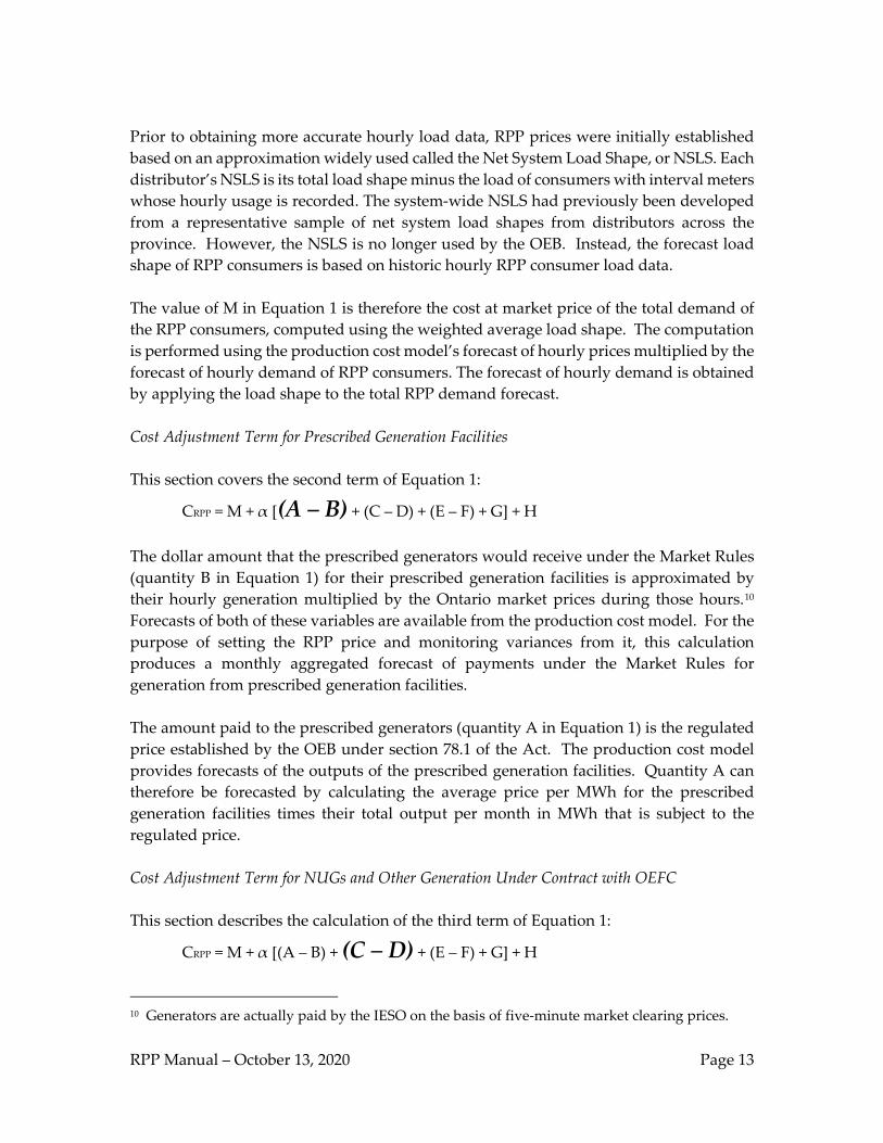
Prior to obtaining more accurate hourly load data, RPP prices were initially established based on an approximation widely used called the Net System Load Shape, or NSLS. Each distributor’s NSLS is its total load shape minus the load of consumers with interval meters whose hourly usage is recorded. The system-wide NSLS had previously been developed from a representative sample of net system load shapes from distributors across the province. However, the NSLS is no longer used by the OEB. Instead, the forecast load shape of RPP consumers is based on historic hourly RPP consumer load data. The value of M in Equation 1 is therefore the cost at market price of the total demand of the RPP consumers, computed using the weighted average load shape. The computation is performed using the production cost model’s forecast of hourly prices multiplied by the forecast of hourly demand of RPP consumers. The forecast of hourly demand is obtained by applying the load shape to the total RPP demand forecast. Cost Adjustment Term for Prescribed Generation Facilities This section covers the second term of Equation 1:
CRPP = M + α [(A – B) + (C – D) + (E – F) + G] + H The dollar amount that the prescribed generators would receive under the Market Rules (quantity B in Equation 1) for their prescribed generation facilities is approximated by their hourly generation multiplied by the Ontario market prices during those hours.10 Forecasts of both of these variables are available from the production cost model. For the purpose of setting the RPP price and monitoring variances from it, this calculation produces a monthly aggregated forecast of payments under the Market Rules for generation from prescribed generation facilities. The amount paid to the prescribed generators (quantity A in Equation 1) is the regulated price established by the OEB under section 78.1 of the Act. The production cost model provides forecasts of the outputs of the prescribed generation facilities. Quantity A can therefore be forecasted by calculating the average price per MWh for the prescribed generation facilities times their total output per month in MWh that is subject to the regulated price. Cost Adjustment Term for NUGs and Other Generation Under Contract with OEFC This section describes the calculation of the third term of Equation 1:
CRPP = M + α [(A – B) + (C – D) + (E – F) + G] + H
10 Generators are actually paid by the IESO on the basis of five-minute market clearing prices.
RPP Manual – October 13, 2020 Page 14
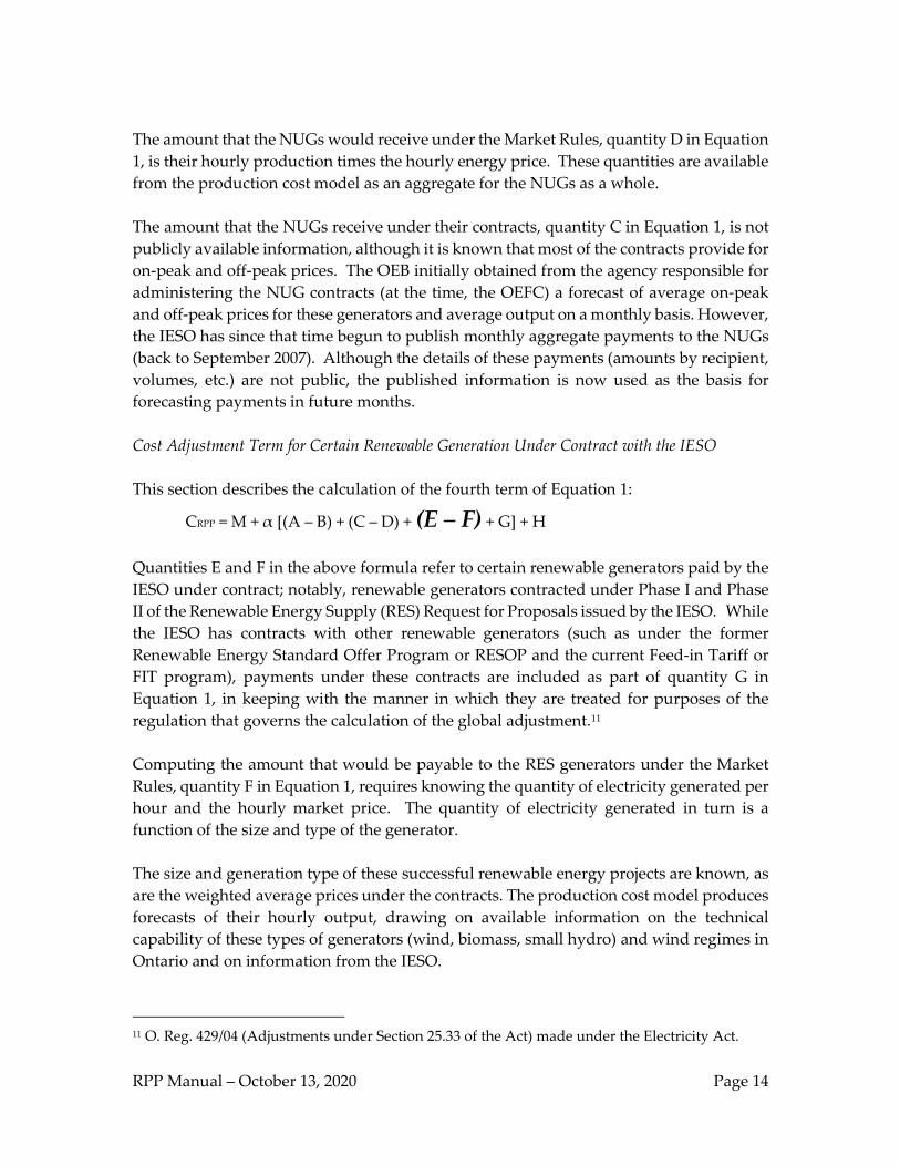
The amount that the NUGs would receive under the Market Rules, quantity D in Equation 1, is their hourly production times the hourly energy price. These quantities are available from the production cost model as an aggregate for the NUGs as a whole. The amount that the NUGs receive under their contracts, quantity C in Equation 1, is not publicly available information, although it is known that most of the contracts provide for on-peak and off-peak prices. The OEB initially obtained from the agency responsible for administering the NUG contracts (at the time, the OEFC) a forecast of average on-peak and off-peak prices for these generators and average output on a monthly basis. However, the IESO has since that time begun to publish monthly aggregate payments to the NUGs (back to September 2007). Although the details of these payments (amounts by recipient, volumes, etc.) are not public, the published information is now used as the basis for forecasting payments in future months. Cost Adjustment Term for Certain Renewable Generation Under Contract with the IESO This section describes the calculation of the fourth term of Equation 1:
CRPP = M + α [(A – B) + (C – D) + (E – F) + G] + H Quantities E and F in the above formula refer to certain renewable generators paid by the IESO under contract; notably, renewable generators contracted under Phase I and Phase II of the Renewable Energy Supply (RES) Request for Proposals issued by the IESO. While the IESO has contracts with other renewable generators (such as under the former Renewable Energy Standard Offer Program or RESOP and the current Feed-in Tariff or FIT program), payments under these contracts are included as part of quantity G in Equation 1, in keeping with the manner in which they are treated for purposes of the regulation that governs the calculation of the global adjustment.11 Computing the amount that would be payable to the RES generators under the Market Rules, quantity F in Equation 1, requires knowing the quantity of electricity generated per hour and the hourly market price. The quantity of electricity generated in turn is a function of the size and type of the generator. The size and generation type of these successful renewable energy projects are known, as are the weighted average prices under the contracts. The production cost model produces forecasts of their hourly output, drawing on available information on the technical capability of these types of generators (wind, biomass, small hydro) and wind regimes in Ontario and on information from the IESO.
11 O. Reg. 429/04 (Adjustments under Section 25.33 of the Act) made under the Electricity Act.

RPP Manual – October 13, 2020 Page 15
Cost Adjustment Term for Other Contracts with the IESO and for OEB-approved CDM Programs This section describes the calculation of the fifth term of Equation 1:
CRPP = M + α [(A – B) + (C – D) + (E – F) + G] + H Currently included in G are the following:
i. generation facilities procured under the 2005 “Clean Energy Supply” RFP (including the Greenfield Energy Centre and St. Clair Power gas-fired facilities);
ii. the “refurbishment” contract with Bruce Power;
iii. the so-called “early mover” clean energy supply contracts;
iv. contracts issued under the former RESOP program;
v. certain other generation contracts (including those awarded through the
Combined Heat and Power (CHP) RFP and the contract for supply from the Portlands gas-fired facility);
vi. various contracts for the supply of demand response or conservation and
demand-side management;
vii. contracts issued under the FIT program; and
viii. amounts for CDM programs administered by the IESO. Generation Contracts The contribution of generation under contract to the IESO to quantity G in Equation 1 depends on the size, type and technical capability of the generators, on market conditions, and on their contracts with the IESO. Only the contractual compensation contributes to quantity G. In terms of information that is not publicly available, the OEB obtains from the IESO information at an appropriate level of detail for purposes of enabling the OEB to forecast the contribution of contracted generation to quantity G in Equation 1. With this and other relevant information (such as the forecast of market prices where applicable), the OEB is able to forecast the contribution of the generation under contract to the IESO to quantity G in Equation 1.

RPP Manual – October 13, 2020 Page 16
The Bruce generation facility is subject to a contract effective January 1, 2016 that provides a payment per megawatt hour for all output from its generation site. Other Procurement Contracts The amounts paid by the IESO for these other procurement contracts are forecast as accurately as reasonable given information that is available from public sources as well as information provided to the OEB by the IESO. The IESO provides forecast information on the total amount under contract for demand response and for conservation and demand management, which is the contribution of these contracts to quantity G in Equation 1.12 The OEB estimates the contribution of demand response contracts to quantity G in Equation 1. Amounts for CDM Programs The contribution of CDM programs administered by the IESO to quantity G is estimated based on information from public sources as well as information provided to the OEB by the IESO. Cost for IESO Variance Account This section describes the calculation of the sixth term of Equation 1:
CRPP = M + α [(A – B) + (C – D) + (E – F) + G] + H The IESO incurs direct costs to carry the RPP-related variance account. The IESO must pay interest on any negative variances. The IESO also credits the variance account with interest earned on any positive balances. Interest amounts can be forecast using the forecast of variance over the year and an assumption of the interest rates the IESO would earn or pay, given its credit rating. The IESO does not currently allocate any other specific operating costs to the administration of its RPP-related variance account.
12 Some costs incurred by the IESO in relation to conservation and demand management are not recovered through the global adjustment, such as overhead costs that are recovered through the IESO’s fees and are therefore not captured in determining the RPP supply cost.
RPP Manual – October 13, 2020 Page 17
Total RPP Supply Cost The total RPP supply cost is calculated as the cost of the supply needed to meet the demand from RPP consumers, determined using Equation 1.

RPP Manual – October 13, 2020 Page 18
3. METHODOLOGY AND TIMING FOR SETTING
RPP PRICES
Introduction The diagram in Chapter 1 indicates that setting the base RPP prices integrates two price components. The forward-looking component is based on a forecast of the RPP supply cost, which is calculated as detailed in Chapter 2 of this Manual. The backward-looking component is set to recover the accumulated variance in the IESO variance account. Appendix A describes the equations used to determine the variance component. These two components are then added together to produce the average RPP price, which is referred to as RPA. This chapter explains the processes for calculating and integrating these two components of the base RPP prices. This chapter also describes the process and methodology for setting the tiered prices and seasonal price tiers for consumers that are not being charged on the basis of time-of-use prices, and time-of-use pricing periods (on-peak, off-peak and mid-peak) for those consumers with eligible time-of-use (or smart) meters that are being charged on the basis of time-of-use prices. The contents of this chapter are:
Timing for RPP price setting; Setting the price component to recover the RPP supply cost; Setting the price component to true-up the RPP supply cost variance; Setting the average RPP price; Setting the prices for RPP consumers with conventional meters; Setting the prices and times of application for RPP consumers with eligible time-
of-use meters; and Price true-ups for extraordinary circumstances.
Timing for RPP Price Setting As required by the RPP Regulation, the initial RPP prices were set to be effective for no less than 12 months. Subsequently, the OEB has reviewed and, as required, reset the RPP prices every six months. The price resetting determines how much of a price change is needed to recover both the forecast RPP supply cost and the accumulated variance in the IESO variance account. The default recovery period for the variance account is the next 12 months. The OEB may in special circumstances decide to recover the accumulated variance over a period longer than 12 months.
RPP Manual – October 13, 2020 Page 19
Setting the Price Component to Recover the RPP Supply Cost The first step in the computation of the RPP price is the computation of the forecast RPP supply cost, as described in Chapter 2. The average RPP supply cost is simply the total forecast RPP supply cost for the forecast year divided by the total forecast energy demand of RPP consumers for the year. This price component is not set at the average RPP supply cost; however, it is adjusted to take account of random effects on the costs. Correcting for the Asymmetry in Probabilistic Modeling The actual RPP supply cost is subject to random variation from a number of factors. These factors include, among others, the availability of generation from the prescribed generation facilities,13 the availability of generation from resources under contract to the IESO, the level of demand from consumers taking RPP supply (which varies with the weather), and the load shape of that demand. By their nature, the probability distributions of some of these variables are asymmetric. For example, if the assumed capacity factor of a generator is 80%, then there is more possible downside (to 0%) than upside (to 100%). Some other variables have similarly skewed distributions. Based on the above, probabilistic modeling of the variance of actual from forecast RPP supply cost shows that there is a higher probability that the actual RPP supply cost will be above its expected value than below it. This raises the probability that such variance will trigger the need for multiple mid-plan price adjustments. A stochastic adjustment is calculated using a probabilistic simulation of the system (Monte Carlo technique) to determine the size of the variance given assumptions about the level of price and the distributions of the variables that drive market price determination. The stochastic adjustment has remained relatively constant since the RPP was introduced, adding about $1 / MWh to the RPP price.
Setting the Price Component to True-Up RPP Supply Cost Variance The total RPP supply cost variance is the difference between the actual RPP supply cost in a year and the amount collected from RPP consumers during that year. This amount is accumulated and held by the IESO in a variance account, and is tracked and monitored monthly by the OEB as described in Chapter 4 of this Manual.
13 As noted earlier, this refers to those of OPG’s regulated nuclear and hydroelectric generation assets that are identified in O. Reg. 53/05 (Payments under Section 78.1 of the Act).
RPP Manual – October 13, 2020 Page 20
The variance is forecast for each month of the RPP year. At the end of each month there will therefore be a forecast and an actual variance amount. The difference between these is called the unexpected variance for the month. The RPP price is normally designed so theexpected cumulative variance is zero at the end of the RPP year. For any shorter period, the forecast cumulative variance will not be zero, since the variance is expected to display a seasonal pattern. Consumer debit variances are expected to accumulate in lower-volume (spring and summer) seasons and consumer credit variances are expected to accumulate in the generally higher-volume (winter and summer) seasons. Only when there is an unexpected cumulative consumer credit or debit balance at the time of a price resetting will it mean that the price should be trued up to recover that deviation; that is, the relevant amount for the true-up is not the actual accumulated variance, but the accumulated difference between the actual variance and the expected variance. In other words, the amount to be trued up is limited to the unexpected variance. Normally, this accumulated unexpected variance is to be recovered over the 12 months following the date of the price setting. The component of the RPP price for recovery of this accumulated unexpected variance is therefore the total of the accumulated unexpected variance divided by the forecast energy demand of RPP consumers over the succeeding 12 months. In special circumstances, the OEB may decide to set the RPP price with a view to recovering the variance over a period longer than 12 months, i.e., to defer the recovery of a portion of the variance until after the 12-month RPP price-setting period.14 In determining whether special circustances exist the OEB will be guided by its statutory objectives, and particularly the objective to protect consumers with respect to prices.
Setting the Average RPP Price The average RPP price is therefore the sum of these two components:
1. The prospective recovery of the forecast RPP supply cost; and 2. The retrospective recovery of the cumulative unexpected variance.
This average RPP price is denoted as RPA. The next steps in the price-setting process determine the prices to be charged to each group of RPP consumers; (i) those that are charged on the basis of time-of-use prices; and (ii) those that are charged on the basis of tiered prices.
14 Previously, subsection 79.16(3) of the OEB Act required the OEB to set prices “within 12 months or such shorter time periods as the Minister may direct”; in 2017, that provision was repealed.

RPP Manual – October 13, 2020 Page 21
Setting the Tiered Prices For RPP consumers that are not on time-of-use pricing, the OEB has established a tiered pricing structure. The tier structure includes both the levels of the prices in the two tiers — RPCMT1 (the price for consumption at or below the tier threshold) and RPCMT2 (the price for consumption above the tier threshold) — and the threshold level of consumption at which the consumer’s price will move from the lower to the higher tier. The tier prices, RPCMT1 and RPCMT2, are the same for all RPP consumers. However, the tier thresholds are not the same at all times, as stated in section 3.3.2 of the SSS code. The tier prices must be calculated so that the expected average price, calculated on a “tier load weighted” basis, equals the average RPP price, RPA. Given the tier threshold, the amount of electricity expected to be priced at each tier can be estimated. For that estimation, the OEB uses information showing how much electricity consumers purchase in each month at each of the tiers. That calculation assumes that the tier thresholds are the same for all RPP consumers. The OEB then calculates the tier prices by targeting a ratio of 0.85 between the upper and lower tier prices. This ratio of 0.85 was selected when the OEB initially set RPP prices based on the then-existing tiered price structure established by the government (the prices at that time were 4.7 cents for consumption at or below the tier and 5.5 cents for consumption above the tier). For the actual calculation, the OEB uses information on monthly consumption volumes. This Manual now addresses the threshold for residential consumers. Since November 1, 2005, and as contemplated in section 3.3.2 of the SSS Code, the threshold has changed seasonally, with two six-month seasons starting on November 1 and May 1. The tier thresholds for residential consumers have normally been set at 1000 kWh per month in the winter season (November 1 to April 30) and 600 kWh per month in the summer season (May 1 to October 31). These thresholds were selected based on information regarding the amount of electricity that consumers use in each of the heating and non-heating months. For non-residential consumers, the threshold has been fixed at 750 kWh per month all year round. Although section 3.3.2 of the SSS Code contemplates that the OEB may vary that threshold, to date it has not done so.
RPP Manual – October 13, 2020 Page 22
Setting the Time-of-Use Prices This section explains the methodology for computing the prices for RPP consumers with eligible time-of-use (or smart) meters that have not elected to be charged on the basis of tiered prices.15 Time-of-use prices are set to make the forecast average price charged to consumers that are being billed on the basis of those prices equal to RPA, the average RPP price. The basic methodology for determining the time-of-use prices, the values of RPEMOFF (price during an off-peak period), RPEMMID (price during a mid-peak period), and RPEMON (price during an on-peak period) is to use data from the forecast cost of RPP supply and the forecast demand for such consumers to determine a set of prices that reflects their supply cost and that averages to RPA. Time-of-use prices differ according to the season and time of day. The level of these prices is connected to the times when these prices apply because the cost of supplying electricity varies according to when it is supplied. Objectives and Choices Setting time-of-use prices requires more steps and more decisions than setting tiered prices. The complexity arises from the requirement to set more prices and the time periods when these prices will apply. One of the objectives of having time-of-use meters is to give consumers more precise price signals and incentives to respond to those price signals. Consumers that are billed on the basis of time-of-use prices see prices that differ during the day, reflecting relative costs of generation at different times and allowing consumers to benefit by shifting or changing their consumption in response. Similar to the tiered prices, time-of-use prices are fixed in advance in order to limit the consumer’s exposure to supply price volatility and to provide all RPP consumers with predictable prices. The objectives for the time-of-use pricing system include: Set prices to recover the full cost of RPP supply, on a forecast basis, from the
consumers who pay the prices; Set the price structure to reflect current and future RPP supply costs; Set the price structure to support the achievement of efficient electricity system
operation and investment;
15 As of November 1, 2020, RPP consumers who would otherwise be charged on the basis of time-of-use prices may elect instead to be charged on the basis of tiered prices by giving notice to their distributor: see subsection 6(4) of the RPP Regulation and section 3.5 of the Standard Supply Service Code.
RPP Manual – October 13, 2020 Page 23
Set both prices and the price structure to give consumers incentives and opportunities to reduce their electricity bills by shifting their time of electricity use and reducing their peak demand;
Create a price structure that is easily understood by consumers; and Provide fair, stable and predictable commodity prices to consumers.
These objectives guide the choices to be made to determine the prices. Some choices are reflected in the SSS Code. The most important of these are that there are three price levels and that there may be two seasons. The choices not articulated in the SSS Code include: The times of day at which the three price levels (RPEMOFF, RPEMMID, and RPEMON)
apply: o Whether the times will differ in different seasons (and if so, how) o Whether the times will differ by day of the week (weekday vs. weekend);
and The three price levels (RPEMOFF, RPEMMID, and RPEMON).
Determination of the Number of Time-of-Use Periods The number of time-of-use periods should be chosen to further the objective of making the prices reflect the changes in supply costs over time in the Ontario electricity market. Since the prices are based on forecasts, the pattern of seasonal prices can also be based on forecasts. The number of time-of-use periods was initially determined by the OEB based on the forecast of hourly HOEP, by season, for the first year of the RPP, as described in the initial version of this Manual:
Figure 4 below shows the forecast of hourly HOEP, by season, for the first year of the RPP. Prices are the forecast HOEP for the hour of day ending at the hour shown on the horizontal axis. The price points are plotted in the middle of the hourly intervals shown and reflect the average HOEP during that interval. Note that the hours and the average HOEP for the summer season in Figure 4 have been adjusted for daylight savings time (i.e., times are given in Eastern Daylight Savings Time for the summer season and in Eastern Standard Time for the winter season).

RPP Manual – October 13, 2020 Page 24
Figure 4: Forecast Seasonal HOEP
Source: Navigant Consulting
The chart shows some consistency and some difference in the daily patterns of forecast prices in the two seasons.
Winter prices show a pronounced daily peak in the early evening hours, corresponding to residential and commercial lighting and space heating uses, and to residential appliance use. The winter evening peak price lasts from roughly 5 p.m. to 9 p.m. There is an almost equal peak period in the early morning hours, again reflecting commercial and residential lighting and space heating, and residential appliance use. The morning peak period lasts from about 7 a.m. to 11 a.m. While the highest prices in the morning are not as high as the highest evening peak prices, they are noticeably higher than those in the middle of the day. Winter therefore shows a noticeable daily double peak pattern.
In the summer, prices start to rise at about the same time as they do in the winter, about 7 a.m., but the most pronounced peak period is spread out over the afternoon, lasting from about 11 a.m. to 5 p.m. This corresponds to residential and commercial air-conditioning use on the hottest summer days. Accordingly,
$0
$20
$40
$60
$80
$100
$120
1 2 3 4 5 6 7 8 9 10 11 12 13 14 15 16 17 18 19 20 21 22 23 24
Hour of Day (Ending at Hour Shown)
HO
EP ($
/MW
h)
Winter Weekday (EST)Summer Weekday (EDST)Winter Weekend (EST)Summer Weekend (EDST)

RPP Manual – October 13, 2020 Page 25
summer has a single daily peak period. The summer peak prices are close to those of the winter peak, though the averages are somewhat lower.
The pattern of off-peak prices is quite stable for both seasons. Demand falls off sharply after about 11 p.m., and picks up sharply at about 7 a.m.
These data also distinguish between weekdays, weekends and holidays. Weekends and holidays have much lower and much flatter forecast hourly prices because the overall demand is lower and the prices are therefore lower. Because the prices tend to be lower for whole weekends, the entire weekend can be defined as an off-peak period.
The choice of periods for different prices should reflect these patterns of market price, but need not directly replicate them. A price that varies too frequently would jeopardize the RPP goal of price stability.
The data indicate a consistent pattern of low, medium and high prices at specific times of the day and season. The data therefore support a three-price pattern.
A time-of-use pricing structure that comprises three price periods remains appropriate at this time. The OEB’s decision to allocate global adjustment costs non-uniformly across the three price periods (see below) can help mitigate the effects of price convergence between the price periods for RPP price-setting purposes. Times of Application of Prices The next issue is exactly what times to choose to apply the three prices. The time-of-use price periods were also initially determined by the OEB based on the forecast of hourly HOEP, by season, for the first year of the RPP. Subsequent HOEP data shows similar patterns of daily and seasonal variation. All of the weekday prices ramp up rapidly at about 7 a.m., making that time the natural choice for the end of the off-peak period in both summer and winter. Prices ramp down in mid-evening in both winter and summer. Over time, the OEB has made certain changes to the time at which the off-peak period commences on weekday evenings in both winter and summer. In accordance with an amendment to the RPP Regulation,16 effective May 1, 2011 the evening off-peak period must commence no later than 7 p.m. These considerations mean that the peak periods (both mid-peak and on-peak) should be from 7 a.m. to mid-evening (7 p.m.) on weekdays in both winter and summer. Off-peak
16 This amendment was made by O. Reg. 494/10, which came into force on January 1, 2011.

RPP Manual – October 13, 2020 Page 26
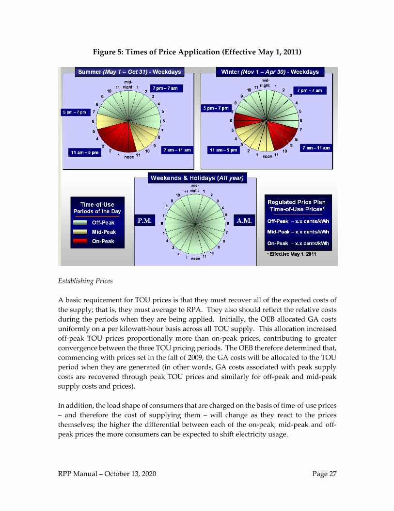
weekday periods are therefore from mid-evening (7 p.m.) to midnight and midnight to 7 a.m. The on-peak periods should reflect the times of distinctly higher prices. Winter has both morning and evening on-peak periods. The morning on-peak period lasts from about 7 a.m. to 11 a.m. or noon, and the evening from 5 p.m. to 8 p.m. or 9 p.m. Prices fall off to the mid-peak levels after 9 p.m., and stay there until they fall again after 10 p.m. or 11 p.m. A reasonable on-peak period for winter weekday mornings is therefore 7 a.m. to 11 a.m. Having regard to the amendment to the RPP Regulation referred to above, the winter weekday evening on-peak period should run from 5 p.m. to 7 p.m. In the summer, the on-peak period for weekdays is from 11 a.m. to 5 p.m. Weekend hours have much the same daily pattern as weekday hours, except that prices tend to be flatter throughout the period from 7 a.m. to 10 p.m. Giving weekends and holidays only off-peak prices would better reflect their cost conditions. Taking these factors into consideration, the time periods for time-of-use (TOU) price application are defined as follows and as illustrated in Figure 5. Off-peak period (priced at RPEMOFF):
o Winter and summer weekdays: 7 p.m. to midnight and midnight to 7 a.m. o Winter and summer weekends and holidays: 24 hours (all day)
Mid-peak period (priced at RPEMMID) o Winter weekdays (November 1 to April 30): 11 a.m. to 5 p.m. o Summer weekdays (May 1 to October 31): 7 a.m. to 11 a.m. and 5 p.m. to 7 p.m.
On-peak period (priced at RPEMON) o Winter weekdays: 7 a.m. to 11 a.m. and 5 p.m. to 7 p.m. o Summer weekdays: 11 a.m. to 5 p.m.
Times in the summer are local or daylight savings time. For the purpose of RPP time-of-use pricing, a holiday means: New Year’s Day, Family Day, Good Friday, Christmas Day, Boxing Day, Victoria Day, Canada Day, Civic Holiday, Labour Day, and Thanksgiving Day. When any such holiday falls on a weekend (Saturday or Sunday), the next weekday following (that is not also a holiday) is to be treated as the holiday for RPP time-of-use pricing purposes.
RPP Manual – October 13, 2020 Page 27
Figure 5: Times of Price Application (Effective May 1, 2011)
Establishing Prices A basic requirement for TOU prices is that they must recover all of the expected costs of the supply; that is, they must average to RPA. They also should reflect the relative costs during the periods when they are being applied. Initially, the OEB allocated GA costs uniformly on a per kilowatt-hour basis across all TOU supply. This allocation increased off-peak TOU prices proportionally more than on-peak prices, contributing to greater convergence between the three TOU pricing periods. The OEB therefore determined that, commencing with prices set in the fall of 2009, the GA costs will be allocated to the TOU period when they are generated (in other words, GA costs associated with peak supply costs are recovered through peak TOU prices and similarly for off-peak and mid-peak supply costs and prices). In addition, the load shape of consumers that are charged on the basis of time-of-use prices – and therefore the cost of supplying them – will change as they react to the prices themselves; the higher the differential between each of the on-peak, mid-peak and off-peak prices the more consumers can be expected to shift electricity usage.
RPP Manual – October 13, 2020 Page 28
For the calculations necessary to arrive at the TOU prices, it was initially assumed that consumers charged on the basis of those prices have the same load profile as those that are charged on the basis of the tiered prices. However, in 2008, enough data was available from time-of-use meters to begin using a load shape specific to consumers being charged on the basis of TOU prices. To begin the calculation, the load profile of consumers on time-of-use pricing is used to calculate the supply cost for those consumers. This amount is analogous to the RPP supply cost of total demand of participating RPP consumers or quantity M in Equation 1 of Chapter 2. Then this amount is adjusted by the other components of Equation 1. This amount is the RPP supply cost for consumers on time-of-use pricing which must be recovered by the three prices. 17 The key to setting these three prices is that they should reflect sytem value at their times of application, including the specific GA costs associated with each of the TOU periods. TOU prices are based on forecasts, as are the tiered prices. To determine TOU prices, the production cost model price forecast is analyzed to determine average price levels during the different times of application referred to in Figure 5. Then the process can set prices or price ratios to reflect costs. The OEB may supplement the supply cost model forecast with an econometric model based on Ontario market data. This model may be used to determine an initial set of TOU prices which are subsequently adjusted so that these prices recover forecasted supply costs, including GA costs associated with specific TOU periods. After any two of the prices are set, the third price is determined. Forecast prices are required to fully recover the costs of supply, including the specific GA costs associated with peak supply. It is calculated as the price that will meet the forecast supply costs, given the load shape. The price so determined may or may not be fully reflective of the average forecast price in the production cost model during the on-peak hours. Some adjustment may be needed to the other prices to produce a set of three prices that meets the objectives of the time-of-use pricing structure, as set out above. The ratio of the prices has therefore been set in a way that reflects the relative forecast costs from the production cost model for the period for which the prices are being set. An analysis of the forecast data for the first year of the RPP suggested that these prices would occur in the ratio of roughly 1:2:3. This is the relationship that appears in the average forecast prices from those forecasts. That is, the forecast price at the mid-peak times, corresponding to RPEMMID, is roughly twice that at the off-peak times, corresponding to RPEMOFF, and the forecast price at on-peak times, corresponding to RPEMON, is roughly three times RPEMOFF.
17 Currently, the prices are set so that their load-weighted average is equal to RPA.

RPP Manual – October 13, 2020 Page 29
In subsequent years, TOU price forecasts tended to converge, primarily the result of GA costs becoming a greater percentage of total supply costs and being allocated uniformly. In response to this trend and as noted earlier, since November 1, 2009 the OEB has allocated GA costs non-uniformly according to when these costs are generated, i.e., during peak, mid-peak or off-peak hours. Subsequent price settings show that this type of GA cost allocation has offset some of the convergence trend.
Price True-Ups for Extraordinary Circumstances Under some extraordinary circumstances, large unexpected variances (deviations) could accumulate in a short time. This could occur as a result of some major unanticipated event, such as a prolonged unexpected outage of a large generator. As described in Chapter 4 of this Manual, deviations of actual from forecast variances are tracked and monitored monthly. It might be desirable, under such extraordinary circumstances, to take prompt action to bring prices back towards cost to avoid the possibility of accruing undesirably large deviations and, as a result, unusually high price adjustments at the next scheduled RPP price adjustment date.18 In general, it would be expected that such action would not be taken on the basis of one or two months’ experience, but rather would be considered on a quarterly basis. Quarterly analysis smooths the more extreme variations of monthly results, and should therefore avoid making changes in reaction to a relatively short-term extreme event that does not recur. For similar reasons, an interim true-up of this kind should only occur when there has been an extraordinary accumulation of deviations from the expected variance, as indicated by the unexpected variance exceeding a trigger value. Considerations in setting the trigger value include the impact on the consumer bill and the probability of such a high unexpected variance occurring. The trigger value was determined by the OEB in the initial version of this Manual based on the analysis below:
Assuming roughly 4 million RPP consumers, the average cost per customer of a $40 million unexpected variance is about $10. That would have a bill impact of under $1 per month, if collected over 12 months. Variance modeling shows that an unexpected variance of about $40 million a month occurs less than 10% of the time. Choosing a trigger value of $160 million would produce an impact of
18 To be clear, where in the course of setting RPP prices, the OEB decides to defer the recovery of a portion of the accumulated variance beyond the 12-month price-setting period, the remaining variance is not “unexpected” and is not factored in when considering whether the trigger value has been met under the true-up mechanism described here.

RPP Manual – October 13, 2020 Page 30
approximately $40 per customer, and a bill impact of about $3.40 per month. Variance modeling suggests that random events would produce an unexpected variance of that magnitude in a single quarter less frequently than once in five years.
Based on these parameters, the initial trigger value was set at $160 million – about 4% of the total RPP cost in its first year. If the trigger were set today using these same proportions, the trigger would be about $250 million. When a significant unexpected variance, informed by reference to the 4% trigger value, accumulates over a quarter that does not conclude with a scheduled semi-annual true-up and rebasing, the OEB will evaluate whether a price true-up should be implemented in the form of an RPP price adjustment to begin to recover that variance. It is important to clarify that only the unexpected portion of the variance would be included in the RPP price adjustment at that time. The price true-up will be calculated as the total unexpected variance divided by the total forecast RPP demand over the next 12 months. This extraordinary case is the only time that a change in the RPP price is based solely on the need to recover accumulated deviations of the variance from the expected variance (i.e., only retrospective). All ordinary or scheduled RPP price adjustments are based on recovery of both the forecast RPP supply cost and the past accumulated deviations (i.e., both retrospective and prospective).

RPP Manual – October 13, 2020 Page 31
4. METHODOLOGY AND TIMING FOR VARIANCE
TRACKING
Introduction This chapter sets out the methodology and timing for tracking and monitoring the monthly balances19 in the IESO variance account, carried for RPP consumers. The monthly variance balance held by the IESO is the difference between the actual RPP supply cost for the month and the revenues collected from RPP consumers for that month. The actual monthly variance account balance is compared against the expected monthly variance account balance. This chapter describes the methodology and timing for the calculation of the forecast variance and for tracking deviations of actual from forecast variance. Chapter 3 describes the uses of this information for price rebasing and price true-ups. The contents of this chapter are:
Monthly Variances; Variance Forecasting; Variance Monitoring; and Frequency of Variance Monitoring.
Monthly Variances For all RPP consumers, the RPP prices are set in advance for an entire forecast year. The prices reflect a forecast of average RPP supply cost for the forecast year, adjusted to collect any outstanding variance balance at the beginning of the period. The default time periodto bring the expected annual cumulative variance balance as close as technically possible to zero is 12 months. As described in Chapter 3, special circumstances may warrant deferring the recovery of a portion of the variance beyond this 12-month price-setting period).20 In these limited circumstances, the expected variance may be forecast to be something other than zero at the end of 12 months. The actual RPP supply cost in each month can be expected to vary in a systematic way from the forecast average monthly RPP supply cost. This is because both price and demand conditions vary over the year. For example, in the shoulder months, market
19 This discussion is in terms of monthly variances because that is the frequency with which the IESO accumulates variance data. 20 Due to the need to round RPP prices to a tenth of cent, it is not possible to bring the expected variance balance to exactly zero when prices are adjusted.

RPP Manual – October 13, 2020 Page 32
prices will tend to be lower than the annual average, producing a monthly RPP supply cost that is lower than its annual average. In the peak demand months, the market can be expected to produce a monthly RPP supply cost that is higher than its annual average. These considerations lead naturally to the expectation that, in lower-price months, a consumer credit balance can be expected to accumulate in the variance account; in higher-price months, a consumer debit balance can be expected to accumulate in the variance account. Although the average RPP price or RPA is normally chosen to produce a zero expected value of the cumulative variance over the year, the expected value of the variance in each month is not zero. In addition to the normal seasonal trends in consumption patterns discussed above, the residential seasonal tier thresholds also need to be taken into account. While there is only technically a single average RPP price (or RPA), the residential threshold is higher in winter (1000 kWh) than in summer (600 kWh). This means that the average price most tiered price RPP consumers pay will be lower in winter than in summer, since they will have less consumption at the higher tiered price in the winter. Thus, variance clearance will vary from summer to winter. The expected monthly variances can be aggregated into expected quarterly variances, with each quarter representing three months of RPP supply. Figure 6 provides an illustrative example of the possible expected quarterly variances over a single RPP year.
Figure 6: Illustrative Expected Quarterly Variances
The actual RPP supply costs are not expected to exactly match the forecast RPP supply costs, in any given month or quarter, nor are actual RPP revenues expected to exactly match forecast RPP revenues. These differences will create an “unexpected” variance. The term unexpected is used to differentiate this from expected variances that can be forecast
Q1 Q2 Q3 Q4

RPP Manual – October 13, 2020 Page 33
based on expected monthly and seasonal consumption and supply cost patterns. The unexpected variance in a given period is simply the difference between the actual RPP revenue and the actual RPP supply cost less the expected variance for the period. In mathematical terms, the unexpected variance for a given period can be defined as follows: Unexpected Variance = Actual RPP Revenue - Actual RPP Supply Cost - Expected Variance
This is illustrated in Figure 7. In the illustration, the actual variance in the third quarter is greater than the expected variance and the difference between the actual variance and the expected variance is the unexpected variance.
Figure 7: Illustrative Unexpected Quarterly Variances
For the purpose of considering changes in the RPP price, the size of the variance must be monitored. Variances must be trued up so that the actual cost of RPP supply is recovered over time. However, in monitoring the monthly variance, the quantity to be monitored is not the actual variance itself but the unexpected variance in that month. The unexpected variance can be summed over the periods in the year to determine the cumulative unexpected variance. At the end of the year the cumulative unexpected variance and any expected variance will be trued up in the next RPP period.
Variance Forecasting The methodology for setting RPA requires modeling variances of the actual RPP supply cost from the forecast RPP supply cost. For that purpose, a probabilistic model is constructed which models the events that can produce variances from the forecast RPP supply cost, given assumptions about the probability distribution of the key driving
Q1 Q2 Q3 Q4
ExpectedActualUnexpected Variance

RPP Manual – October 13, 2020 Page 34
variables. The model results are then used to establish the expected value of the variance. This variance model is the basis for the forecast of expected monthly variances. A monthly variance forecast is produced every six months each time that RPP prices are reset because variance modeling is done at that time. The variance forecast uses monthly forecasts of the variables driving the monthly RPP supply cost. These variables include electricity demand and generation availability. These factors are taken at their values from the production cost model, either as inputs to or outputs from that model. The variance model also takes account of the historical volatility of HOEP. These values are then used to produce forecasts of the monthly variance.
Variance Monitoring Two variance totals are calculated and monitored. The first is the cumulative actual variance, as seen in the variance account of the IESO. That amount is the cumulative difference between the actual RPP supply cost and the revenues collected from RPP consumers. It is the amount that must ultimately be collected from consumers, if it is a consumer debit, or paid to them if it is a consumer credit. However, as noted above, recovering that cumulative actual variance amount may not require any additional action. If the cumulative actual variance in any month is the amount forecasted for that month, it will be expected to be offset by variances in the opposite direction in the coming months to result in the expected variance at the end of twelve months from the time of price resetting. For considering true-ups the relevant amount is therefore the unexpected variance. The monthly unexpected variance is monitored for information and to understand trends. The unexpected variance is also accumulated into a quarterly total (as illustrated in Figure7). The quarterly cumulative unexpected variance is also monitored for its potential to trigger an extraordinary true-up, as described in Chapter 3. The total cumulative unexpected variance is the amount to be trued up, as described in Chapter 3 of this Manual. Appendix A describes the equations used to determine the total cumulative unexpected variance.
Frequency of Variance Monitoring The process described above occurs monthly. The actual cumulative variance is available on a monthly basis from the IESO, and the OEB performs the steps listed in this chapter to monitor its deviation from the forecast for that month.

RPP Manual – October 13, 2020 Page 35
Although the monitoring is monthly, the decision on price resetting and true-ups, as described in Chapter 3 of this Manual, is taken every six months. There is also provision for a true-up as an extraordinary event if the quarterly unexpected variance exceeds a trigger level.

RPP Manual – October 13, 2020 Page 36
5. TIMING FOR RPP PRICE ADJUSTMENTS OR
PRICE STRUCTURE CHANGES
Introduction This chapter sets out how long in advance new RPP prices or changes in RPP price structure will be determined by the OEB prior to the date on which the new prices or structure are to come into effect. This reflects the period of time that distributors will have to implement price level or price structure changes and can be considered as a notification period to distributors. The time periods discussed below are consistent with section 3.8 of the SSS Code, which contains provisions that require distributors to notify RPP consumers of RPP price or price structure changes. New RPP prices are computed at six-month intervals and are the result of an integrated consideration of re-basing and true-ups. Price changes become effective at the beginning of a calendar month. The contents of this chapter are:
Timing of Notification of Price or Price Structure Change; and Timing of Implementation by Distributors.
Timing of Notification of Price or Price Structure Change Most RPP price changes will adjust only the RPP price level(s). For such changes, distributors expect a minimum of about 30 days of lead-time before customers can be billed based on the new RPP price. Since distributors do not start to send out bills to consumers based on the new price until about 15 days after its implementation, the 30-day distributor lead-time is achieved by setting the new prices at least 15 days before the beginning of the month in which the new prices are to be implemented. New prices are therefore set (and distributors are thus informed) generally 15 days before distributors begin charging those new prices to consumers. This applies to changes in any RPP price, namely, to changes to any of RPCMT1, RPCMT2, RPEMOFF, RPEMMID, and RPEMON. This also applies to price changes that are intended to true-up prices as a result of extraordinary circumstances, as described in Chapter 3. Changes to the RPP price structure include changes to tier thresholds21 and any other change affecting an RPP element other than the price level(s). For changes to the RPP price structure, distributors expect 90 days of lead-time, or 75 days before the changes are
21 This does not include the normal seasonal change in the residential tier threshold (600 kWh per month in the summer and 1000 kWh per month in the winter).
RPP Manual – October 13, 2020 Page 37
to be implemented. Therefore, structural changes are targeted to be determined by the OEB (and distributors are thus informed) at least 75 days before their implementation date.
Timing of Implementation by Distributors Distributors will charge RPP consumers based on new RPP prices or a new RPP price structure for consumption on and after the first day of the month of implementation. For some RPP consumers, the first day of the month will not correspond to a meter reading, so the SSS Code permits distributors to pro-rate for the billing period within which the price or price structure change takes effect. The method to be used by distributors for proration is set out in the SSS Code.

RPP Manual – October 13, 2020 Page 38
6. METHODOLOGY FOR DETERMINING FINAL
RPP VARIANCE SETTLEMENT AMOUNTS
Introduction This chapter explains the methodology to be used by distributors to compute final settlement variance amounts for RPP consumers leaving the regulated price plan. This is the methodology referred to in section 3.7.1 of the SSS Code. As shown in Figure 2 of Chapter 1, the IESO carries a variance account representing the accumulated difference between the actual RPP supply cost and the revenues collected from RPP consumers. Consumers who do not leave the RPP will pay or receive the benefit of the accumulated variance over the next 12 months through the component of the RPP price that reflects past variances,22 as described in Chapter 3 of this Manual. However, once consumers leave RPP supply,23 they no longer pay RPP prices and therefore no longer pay or receive the benefit of their share of past cumulative variances. For that reason, these consumers will be responsible for a final RPP variance settlement when they leave RPP supply since the RPP price determination assumed that they would have remained on RPP for the full 12 months. The final RPP variance settlement amount could be positive or negative. In other words, depending on the status of the variance account held by the IESO, the consumer could either receive a payment (i.e., credit) or be required to make a payment (i.e., debit). The contents of this chapter are: Determination of Final RPP Variance Settlement Amount and Rate; and Final RPP Variance Settlement Amount Calculation.
22 RPP consumers are also responsible for paying any interest costs incurred by the IESO in relation to the variance account. A consumer leaving the RPP is also responsible for a share of these interest costs. Equation 2 takes into account that such costs are reported monthly to the OEB and are added to the variance that is reported to the OEB by the IESO each month. 23 That is, move out of Ontario, switch to the spot market option or to a competitive retailer, or cease to be eligible for the RPP.
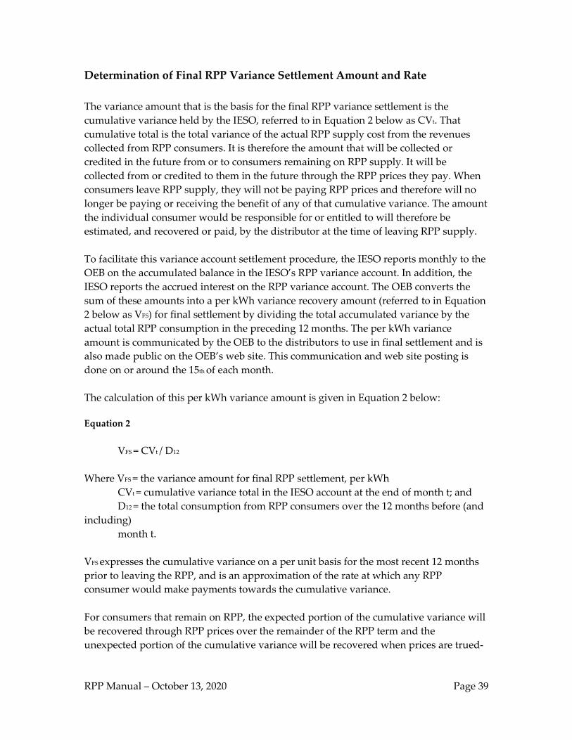
RPP Manual – October 13, 2020 Page 39
Determination of Final RPP Variance Settlement Amount and Rate The variance amount that is the basis for the final RPP variance settlement is the cumulative variance held by the IESO, referred to in Equation 2 below as CVt. That cumulative total is the total variance of the actual RPP supply cost from the revenues collected from RPP consumers. It is therefore the amount that will be collected or credited in the future from or to consumers remaining on RPP supply. It will be collected from or credited to them in the future through the RPP prices they pay. When consumers leave RPP supply, they will not be paying RPP prices and therefore will no longer be paying or receiving the benefit of any of that cumulative variance. The amount the individual consumer would be responsible for or entitled to will therefore be estimated, and recovered or paid, by the distributor at the time of leaving RPP supply. To facilitate this variance account settlement procedure, the IESO reports monthly to the OEB on the accumulated balance in the IESO’s RPP variance account. In addition, the IESO reports the accrued interest on the RPP variance account. The OEB converts the sum of these amounts into a per kWh variance recovery amount (referred to in Equation 2 below as VFS) for final settlement by dividing the total accumulated variance by the actual total RPP consumption in the preceding 12 months. The per kWh variance amount is communicated by the OEB to the distributors to use in final settlement and is also made public on the OEB’s web site. This communication and web site posting is done on or around the 15th of each month. The calculation of this per kWh variance amount is given in Equation 2 below: Equation 2 VFS = CVt / D12
Where VFS = the variance amount for final RPP settlement, per kWh CVt = cumulative variance total in the IESO account at the end of month t; and D12 = the total consumption from RPP consumers over the 12 months before (and including) month t. VFS expresses the cumulative variance on a per unit basis for the most recent 12 months prior to leaving the RPP, and is an approximation of the rate at which any RPP consumer would make payments towards the cumulative variance. For consumers that remain on RPP, the expected portion of the cumulative variance will be recovered through RPP prices over the remainder of the RPP term and the unexpected portion of the cumulative variance will be recovered when prices are trued-
RPP Manual – October 13, 2020 Page 40
up. The amount per kWh that will be recovered is the cumulative variance divided by the forecast of total RPP consumption over the year. Final RPP Variance Settlement Amount Calculation The final variance settlement process collects or credits an appropriate amount from a consumer leaving RPP supply. The amount to be collected or credited in relation to a given consumer is VFS times that consumer’s actual consumption over a specified period of time (the “Final Settlement Consumption Period”). The Final Settlement Consumption Period to be used depends on how long the consumer was on RPP supply before leaving the RPP:
(a) For a consumer that was on RPP supply for a continuous period of 12 months or more, the Final Settlement Consumption Period is the 12 months preceding the consumer’s departure from the RPP.
(b) For a consumer that was on RPP supply for a continuous period of less
than 12 months, the Final Settlement Consumption Period is the actual period during which the consumer was continuously on RPP supply prior to the consumer’s departure from the RPP.
If a distributor does not have a precise total for the consumer’s actual consumption over the applicable Final Settlement Consumption Period, the distributor must reasonably estimate the consumer’s consumption over that period. This must be done by using actual meter readings to the maximum extent possible and interpolating to get an estimate of what the meter reading would have been on the date that corresponds with the beginning of the applicable Final Settlement Consumption Period. Where the consumer that departs the RPP has been a customer of the distributor for less than 12 months, the distributor shall, for the purposes of determining the Final Settlement Consumption Period, take into account the length of the customer’s continuous RPP supply in another service area immediately prior to opening of the customer’s account if that information is known to the distributor. A distributor must collect or credit this final RPP variance settlement amount from each consumer leaving RPP supply under the conditions described in section 3.7.1 of the SSS Code. For this amount then to be properly credited to or debited from the IESO variance account, it must be reported to the IESO under procedures established by the IESO.

RPP Manual – October 13, 2020 Page 41
APPENDIX A: TRUE-UP EQUATIONS This appendix describes the equations used to determine the cost variance component of the process shown in Figure 2 on page 5. The actual variance is always calculated as a cumulative total,
(1) CVt+1 = CVt + Vt,,
Where CVt+1 = actual cumulative variance in time t + 1, CVt = actual cumulative variance in time t, and Vt = actual variance in time t as reported by the IESO.
The cumulative forecast variance is also always calculated as a cumulative total,
(2) FCVt+1 = FCVt + FVt,
Where FCVt+1 = forecast cumulative variance in time t + 1, FCVt = forecast cumulative variance in time t FVt = forecast variance in time t.
Then the unexpected variance in time t is
UVt = FVt – Vt
Where UVt = the unexpected variance in time t. The cumulative unexpected variance is
UCVt+1 = UCVt + UVt
Where UCVt+1 is the cumulative unexpected variance in time t+1. The amount to be trued-up is then always the cumulative unexpected variance at the time of true-up, or UCV6 for a true-up at six months. As discussed in Chapter 3, the OEB may in special circumstances decide to set RPP prices with a view to recovering the variance over a period longer than 12 months, i.e., to defer the recovery of a portion of the variance until after the 12-month RPP price-setting period.