Regularized Evolution for Image Classifier Architecture Search

Esteban Real * 1 Alok Aggarwal * 1 Yanping Huang * 1 Quoc V. Le 1

April 30, 2018

AbstractThe effort devoted to hand-crafting image classi-fiers has motivated the use of architecture searchto discover them automatically. Although evo-lutionary algorithms have been repeatedly ap-plied to architecture search, the architecturesthus discovered have remained inferior to human-crafted ones. Here we show for the first timethat artificially-evolved architectures can matchor surpass human-crafted and RL-designed im-age classifiers. In particular, our models—namedAmoebaNets—achieved a state-of-the-art accu-racy of 97.87% on CIFAR-10 and top-1 accu-racy of 83.1% on ImageNet. Among mobile-sizemodels, an AmoebaNet with only 5.1M parame-ters also achieved a state-of-the-art top-1 accuracyof 75.1% on ImageNet. We also compared thismethod against strong baselines. Finally, we per-formed platform-aware architecture search withevolution to find a model that trains quickly onGoogle Cloud TPUs. This method produced anAmoebaNet that won the Stanford DAWNBenchcompetition for lowest ImageNet training cost.

1. IntroductionUntil recently, most state-of-the-art (SOTA) convolutionalarchitectures have been manually designed by human ex-perts (Krizhevsky et al., 2012; Ciregan et al., 2012; Linet al., 2014; Sermanet et al., 2014; He et al., 2014; Chatfieldet al., 2014; Simonyan & Zisserman, 2015; Karpathy et al.,2014; Szegedy et al., 2015; Donahue et al., 2015; Jader-berg et al., 2015; He et al., 2016; Zagoruyko & Komodakis,2016; Larsson et al., 2017; Huang et al., 2017b; Szegedyet al., 2016; 2017; Xie et al., 2017; Chen et al., 2017; Zhanget al., 2017b; Hu et al., 2018). To speed up the process,researchers have looked into automated methods to discovernew models (Stanley & Miikkulainen, 2002; Stanley et al.,

*Equal contribution 1Google Brain, Mountain View, California,USA. Correspondence to: Esteban Real <ereal@google.com>.

Preliminary work. Copyright 2018 by the author(s).

2009; Andrychowicz et al., 2016; Real et al., 2017; Miikku-lainen et al., 2017; Liu et al., 2018; Zoph et al., 2018; Liuet al., 2017; Zoph & Le, 2016; Baker et al., 2017a; Zhonget al., 2018; Cai et al., 2018; Suganuma et al., 2017; Phamet al., 2018). These methods are now collectively known asarchitecture search algorithms. The traditional approach toarchitecture search is neuro-evolution of topologies (Ange-line et al., 1994; Stanley & Miikkulainen, 2002; Floreanoet al., 2008; Stanley et al., 2009; Fernando et al., 2016; Xie& Yuille, 2017). Improved hardware now allows scalingup these evolutionary algorithms, producing high-qualityimage classification models (Real et al., 2017; Miikkulainenet al., 2017; Liu et al., 2018). Yet, the evolved architectureshave not reached the accuracy and performance of thosedirectly designed by experts.

In this paper, we use a slightly-modified variant of a stan-dard evolutionary algorithm for architecture search. Eacharchitecture is iteratively trained and selected based on howwell it performs on a validation set. The best architecturesat every iteration are allowed to mutate to generate newones, keeping a population of models that improves overtime. In our implementation, the architectures age and dieoff from the population, even if they performed well. Thisaging effect regularizes standard evolution and improvesthe outcome. We applied this algorithm to the NASNetsearch space (Zoph et al., 2018) and found better archi-tectures than those obtained in that study, which used areinforcement-learning (RL) algorithm. In particular, themodel we discovered—named AmoebaNet-C—achieves atop-1 accuracy of 83.1% on ImageNet, matching the currentSOTA, and also sets a new SOTA for small models that canfit on a mobile device.2

We also applied the evolutionary algorithm to find architec-tures that train well on a particular hardware platform. Forthis purpose, we evolved directly on Google Cloud TPUs.The search produced AmoebaNet-B, the new single-modelSOTA on CIFAR-10, with an accuracy of 97.87%, reducing

2Since the writing of this paper, a new study has set a newSOTA on CIFAR-10 and ImageNet by introducing a new data-augmentation technique; they still used AmoebaNet to reach theirImageNet result (Cubuk et al., 2018).

arX

iv:1

802.

0154

8v4

[cs

.NE

] 2

5 Ju

n 20

18

Regularized Evolution

the error from the previous leading result by 8%. We thenran evolution on ImageNet directly and manually extrapo-lated the changes the evolutionary process was making, toproduce AmoebaNet-D. An implementation of AmoebaNet-D won the Stanford DAWNBench competition for the lowestImageNet training cost (Coleman et al., 2017). In particular,that implementation cost $49.30 to reach 93% top-5 accu-racy. This is 16% better than the second-best model in thecompetition, which was ResNet and which trained on thesame hardware3.

2. Related WorkIn recent years, progress has been made in automatingthe process of searching for good architectures, especiallyfor image classification. In fact, some recent ImageNetSOTA results had been obtained by using learning-basedapproaches (Zoph et al., 2018; Liu et al., 2017), after a se-ries of studies exploring these methods (Zoph & Le, 2016;Baker et al., 2017a; Zoph et al., 2018; Zhong et al., 2018;Cai et al., 2018).

Some approaches stand out due to their efficiency (Zhonget al., 2018; Suganuma et al., 2017; Pham et al., 2018).This is important because reducing compute cost is one ofthe main challenges of architecture search. This efficiency,however, may not be entirely due to their algorithm—asmaller search space can help significantly, for example.Platform-aware optimization is a viable approach (Donget al., 2018). Also, while some got very close to the SOTA(Zhong et al., 2018), actually reaching it might require muchmore compute power, as it did in some studies (Zoph et al.,2018; Liu et al., 2017). Diminishing accuracy returns at thehigh-resource regime would not be surprising.

Architecture search speed can be improved with a varietyof techniques: progressive-complexity search stages (Liuet al., 2017), hypernets (Brock et al., 2018), accuracy predic-tion (Baker et al., 2017b; Klein et al., 2017; Domhan et al.,2017), warm-starting and ensembling (Feurer et al., 2015),parallelization, reward shaping and early stopping (Zhonget al., 2018) or Net2Net transformations (Cai et al., 2018).Most of these methods could in principle be applied to evo-lution too. (Miikkulainen et al., 2017) took the orthogonalstrategy of splitting up the search into two different modelscales in two co-evolving populations, showing benefits.

The regularization technique employed removes the oldestmodel from a population undergoing tournament selection.This has precedent in generational evolutionary algorithms,which discard all models at regular intervals (Miikkulainenet al., 2017; Xie & Yuille, 2017; Suganuma et al., 2017).We avoided such generational algorithms due to their syn-

3The Stanford DAWNBench public leaderboard can be foundat https://dawn.cs.stanford.edu/benchmark/#imagenet-train-cost

chronous nature. Tournament selection is asynchronous.This makes it more resource efficient and so it was recentlyused in its non-regularized form for large-scale evolution(Real et al., 2017; Liu et al., 2018). Yet, when it was intro-duced decades ago, it had a regularizing element—albeita more complex one: sometimes a random individual wasselected (Goldberg & Deb, 1991); no individuals were re-moved. Removal may be desirable for garbage-collectionpurposes. The version in (Real et al., 2017) removes theworst individual, which is not regularizing. The version weuse is regularized, natural, and permits garbage collection.

Other than through evolution and RL, architecture searchwas also explored with cascade-correlation (Fahlman &Lebiere, 1990), boosting (Cortes et al., 2017; Huang et al.,2017a), hill-climbing (Elsken et al., 2017), MCTS (Ne-grinho & Gordon, 2017), SMBO (Mendoza et al., 2016;Liu et al., 2017), random search (Bergstra & Bengio, 2012)and grid search (Zagoruyko & Komodakis, 2016). Someeven forewent the idea of individual architectures (Saxena& Verbeek, 2016; Fernando et al., 2017) and some used evo-lution to train a single architecture (Jaderberg et al., 2017)or to find its weights (Such et al., 2017). There is mucharchitecture search work beyond image classification too,but we could not do it justice here.

3. Methods3.1. Search Space

All experiments use the NASNet search space which haspreviously been used to design high-quality models withan RL algorithm in the baseline study, Zoph et al. (2018).The goal is to discover the architectures of two Inception-like modules, called the normal cell and the reduction cell,which preserve and reduce input size, respectively. Thesecells are stacked in feed-forward patterns to form imageclassifiers. The resulting models have two hyper-parametersthat control their size and impact their accuracy: convolutionchannel depth (F) and cell stacking depth (N). We only usedthese parameters only to trade accuracy against size, soknowledge of their existence suffices here and we refer thereader to the baseline study for other details.

During the search phase, only the structure of the cells canbe altered. These cells each look like a graph with C verticesor combinations. A single combination takes two inputs,applies an operation (op) to each, and then adds them togenerate an output. All unused outputs are concatenated toform the final output of the cell. (More details in the Sup-plementary Material, Section S-1.1; examples in Figure 2).

3.2. Regularized Evolution for Architecture Search

The evolutionary algorithm is a variant of the standard tour-nament selection method (Goldberg & Deb, 1991). In our

Regularized Evolution

0 20k# Models Searched0.89

0.92

Mean T

est

ing A

ccura

cy

Evolution

RL

RS

0.75 1.35Billion FLOPs0.957

0.967

Test

ing A

ccura

cy

Evol.

RL

RS

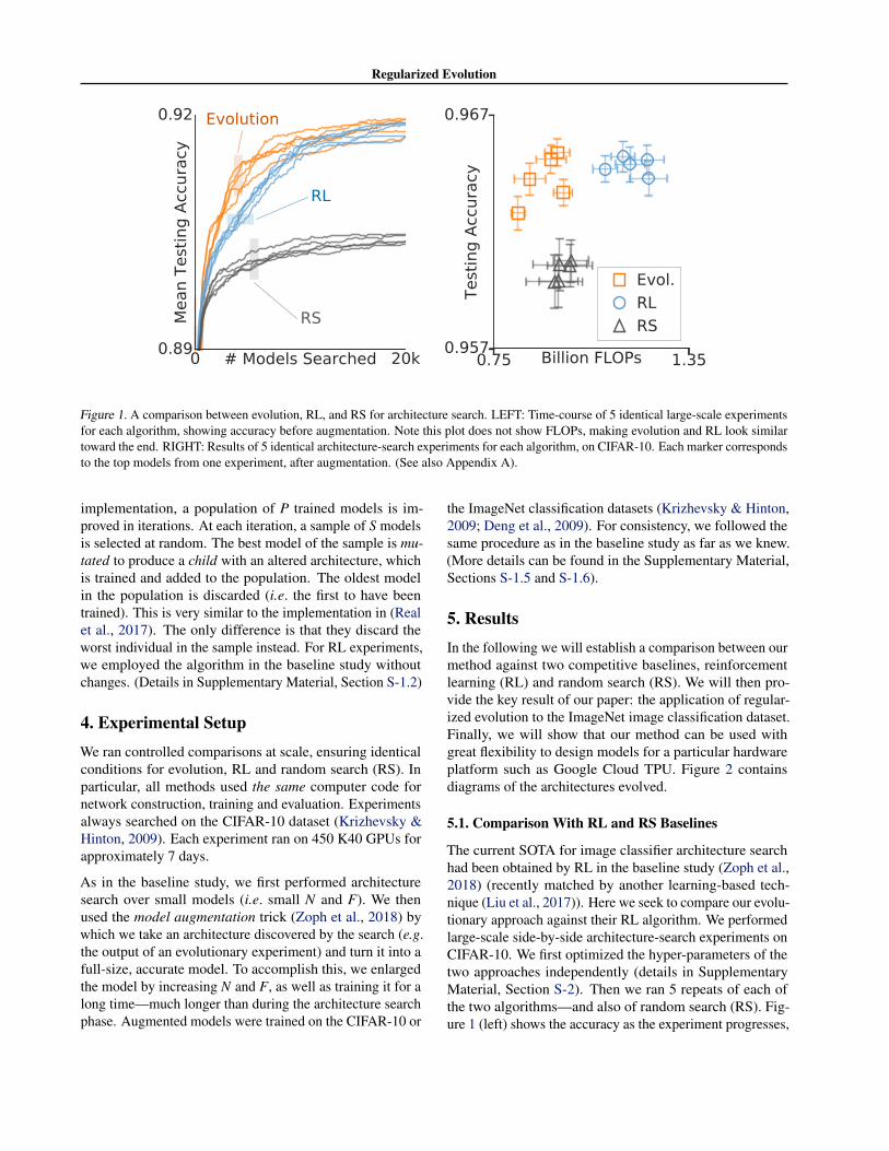
Figure 1. A comparison between evolution, RL, and RS for architecture search. LEFT: Time-course of 5 identical large-scale experimentsfor each algorithm, showing accuracy before augmentation. Note this plot does not show FLOPs, making evolution and RL look similartoward the end. RIGHT: Results of 5 identical architecture-search experiments for each algorithm, on CIFAR-10. Each marker correspondsto the top models from one experiment, after augmentation. (See also Appendix A).

implementation, a population of P trained models is im-proved in iterations. At each iteration, a sample of S modelsis selected at random. The best model of the sample is mu-tated to produce a child with an altered architecture, whichis trained and added to the population. The oldest modelin the population is discarded (i.e. the first to have beentrained). This is very similar to the implementation in (Realet al., 2017). The only difference is that they discard theworst individual in the sample instead. For RL experiments,we employed the algorithm in the baseline study withoutchanges. (Details in Supplementary Material, Section S-1.2)

4. Experimental SetupWe ran controlled comparisons at scale, ensuring identicalconditions for evolution, RL and random search (RS). Inparticular, all methods used the same computer code fornetwork construction, training and evaluation. Experimentsalways searched on the CIFAR-10 dataset (Krizhevsky &Hinton, 2009). Each experiment ran on 450 K40 GPUs forapproximately 7 days.

As in the baseline study, we first performed architecturesearch over small models (i.e. small N and F). We thenused the model augmentation trick (Zoph et al., 2018) bywhich we take an architecture discovered by the search (e.g.the output of an evolutionary experiment) and turn it into afull-size, accurate model. To accomplish this, we enlargedthe model by increasing N and F, as well as training it for along time—much longer than during the architecture searchphase. Augmented models were trained on the CIFAR-10 or

the ImageNet classification datasets (Krizhevsky & Hinton,2009; Deng et al., 2009). For consistency, we followed thesame procedure as in the baseline study as far as we knew.(More details can be found in the Supplementary Material,Sections S-1.5 and S-1.6).

5. ResultsIn the following we will establish a comparison between ourmethod against two competitive baselines, reinforcementlearning (RL) and random search (RS). We will then pro-vide the key result of our paper: the application of regular-ized evolution to the ImageNet image classification dataset.Finally, we will show that our method can be used withgreat flexibility to design models for a particular hardwareplatform such as Google Cloud TPU. Figure 2 containsdiagrams of the architectures evolved.

5.1. Comparison With RL and RS Baselines

The current SOTA for image classifier architecture searchhad been obtained by RL in the baseline study (Zoph et al.,2018) (recently matched by another learning-based tech-nique (Liu et al., 2017)). Here we seek to compare our evolu-tionary approach against their RL algorithm. We performedlarge-scale side-by-side architecture-search experiments onCIFAR-10. We first optimized the hyper-parameters of thetwo approaches independently (details in SupplementaryMaterial, Section S-2). Then we ran 5 repeats of each ofthe two algorithms—and also of random search (RS). Fig-ure 1 (left) shows the accuracy as the experiment progresses,

Regularized Evolution

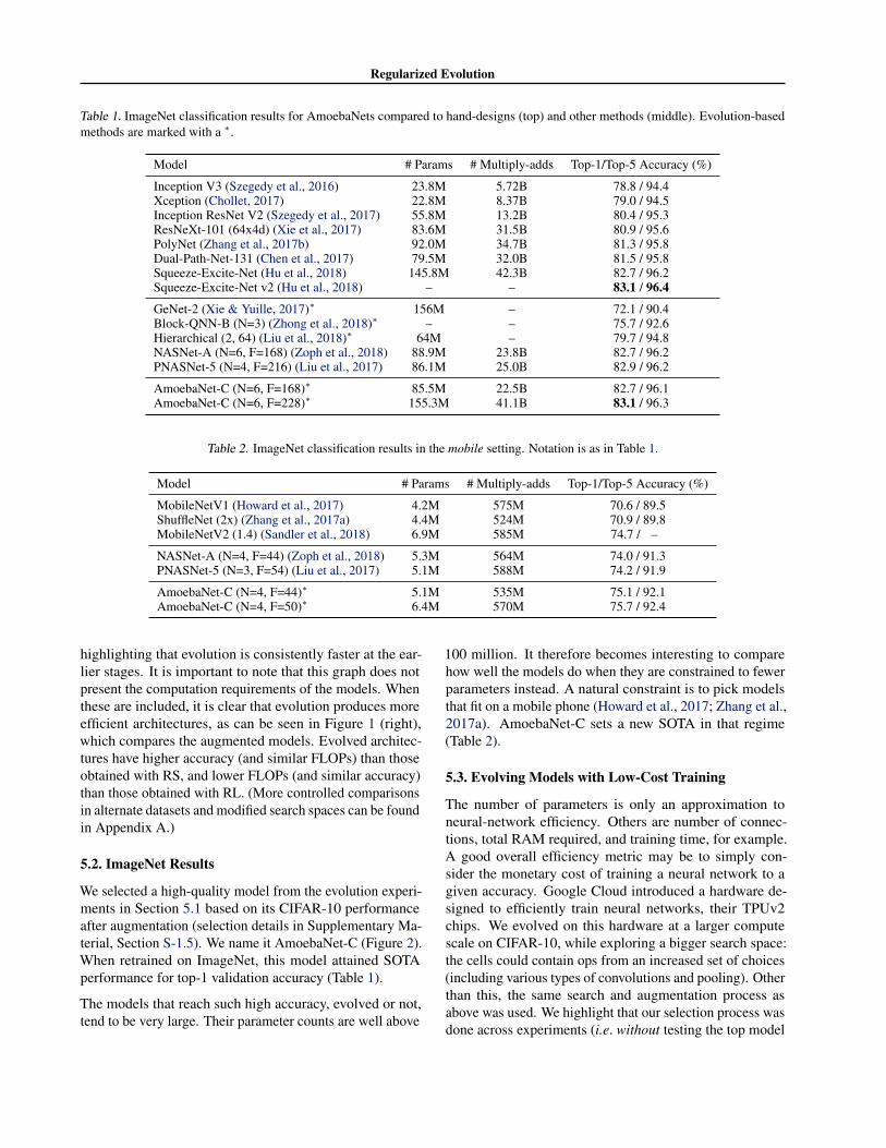
Table 1. ImageNet classification results for AmoebaNets compared to hand-designs (top) and other methods (middle). Evolution-basedmethods are marked with a ∗.

Model # Params # Multiply-adds Top-1/Top-5 Accuracy (%)

Inception V3 (Szegedy et al., 2016) 23.8M 5.72B 78.8 / 94.4Xception (Chollet, 2017) 22.8M 8.37B 79.0 / 94.5Inception ResNet V2 (Szegedy et al., 2017) 55.8M 13.2B 80.4 / 95.3ResNeXt-101 (64x4d) (Xie et al., 2017) 83.6M 31.5B 80.9 / 95.6PolyNet (Zhang et al., 2017b) 92.0M 34.7B 81.3 / 95.8Dual-Path-Net-131 (Chen et al., 2017) 79.5M 32.0B 81.5 / 95.8Squeeze-Excite-Net (Hu et al., 2018) 145.8M 42.3B 82.7 / 96.2Squeeze-Excite-Net v2 (Hu et al., 2018) – – 83.1 / 96.4

GeNet-2 (Xie & Yuille, 2017)∗ 156M – 72.1 / 90.4Block-QNN-B (N=3) (Zhong et al., 2018)∗ – – 75.7 / 92.6Hierarchical (2, 64) (Liu et al., 2018)∗ 64M – 79.7 / 94.8NASNet-A (N=6, F=168) (Zoph et al., 2018) 88.9M 23.8B 82.7 / 96.2PNASNet-5 (N=4, F=216) (Liu et al., 2017) 86.1M 25.0B 82.9 / 96.2

AmoebaNet-C (N=6, F=168)∗ 85.5M 22.5B 82.7 / 96.1AmoebaNet-C (N=6, F=228)∗ 155.3M 41.1B 83.1 / 96.3

Table 2. ImageNet classification results in the mobile setting. Notation is as in Table 1.

Model # Params # Multiply-adds Top-1/Top-5 Accuracy (%)

MobileNetV1 (Howard et al., 2017) 4.2M 575M 70.6 / 89.5ShuffleNet (2x) (Zhang et al., 2017a) 4.4M 524M 70.9 / 89.8MobileNetV2 (1.4) (Sandler et al., 2018) 6.9M 585M 74.7 / –

NASNet-A (N=4, F=44) (Zoph et al., 2018) 5.3M 564M 74.0 / 91.3PNASNet-5 (N=3, F=54) (Liu et al., 2017) 5.1M 588M 74.2 / 91.9

AmoebaNet-C (N=4, F=44)∗ 5.1M 535M 75.1 / 92.1AmoebaNet-C (N=4, F=50)∗ 6.4M 570M 75.7 / 92.4

highlighting that evolution is consistently faster at the ear-lier stages. It is important to note that this graph does notpresent the computation requirements of the models. Whenthese are included, it is clear that evolution produces moreefficient architectures, as can be seen in Figure 1 (right),which compares the augmented models. Evolved architec-tures have higher accuracy (and similar FLOPs) than thoseobtained with RS, and lower FLOPs (and similar accuracy)than those obtained with RL. (More controlled comparisonsin alternate datasets and modified search spaces can be foundin Appendix A.)

5.2. ImageNet Results

We selected a high-quality model from the evolution experi-ments in Section 5.1 based on its CIFAR-10 performanceafter augmentation (selection details in Supplementary Ma-terial, Section S-1.5). We name it AmoebaNet-C (Figure 2).When retrained on ImageNet, this model attained SOTAperformance for top-1 validation accuracy (Table 1).

The models that reach such high accuracy, evolved or not,tend to be very large. Their parameter counts are well above

100 million. It therefore becomes interesting to comparehow well the models do when they are constrained to fewerparameters instead. A natural constraint is to pick modelsthat fit on a mobile phone (Howard et al., 2017; Zhang et al.,2017a). AmoebaNet-C sets a new SOTA in that regime(Table 2).

5.3. Evolving Models with Low-Cost Training

The number of parameters is only an approximation toneural-network efficiency. Others are number of connec-tions, total RAM required, and training time, for example.A good overall efficiency metric may be to simply con-sider the monetary cost of training a neural network to agiven accuracy. Google Cloud introduced a hardware de-signed to efficiently train neural networks, their TPUv2chips. We evolved on this hardware at a larger computescale on CIFAR-10, while exploring a bigger search space:the cells could contain ops from an increased set of choices(including various types of convolutions and pooling). Otherthan this, the same search and augmentation process asabove was used. We highlight that our selection process wasdone across experiments (i.e. without testing the top model

Regularized Evolution

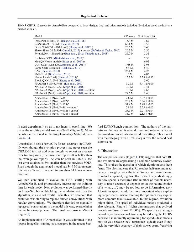
Table 3. CIFAR-10 results for AmoebaNets compared to hand-designs (top) and other methods (middle). Evolution-based methods aremarked with a ∗.

Model # Params Test Error (%)

DenseNet-BC (k = 24) (Huang et al., 2017b) 15.3 M 3.62ResNeXt-29, 16x64d (Xie et al., 2017) 68.1 M 3.58DenseNet-BC (L=100, k=40) (Huang et al., 2017b) 25.6 M 3.46Shake-Shake 26 2x96d (Gastaldi, 2017) + cutout (DeVries & Taylor, 2017) 26.2 M 2.56PyramidNet + Shakedrop (Han et al., 2016; Yamada et al., 2018) 26.0 M 2.31

Evolving DNN (Miikkulainen et al., 2017)∗ – 7.30MetaQNN (top model) (Baker et al., 2017a) – 6.92CGP-CNN (ResSet) (Suganuma et al., 2017)∗ 1.68 M 5.98Large Scale Evolution (Real et al., 2017)∗ 5.4 M 5.40EAS (Cai et al., 2018) 23.4 M 4.23SMASHv2 (Brock et al., 2018) 16 M 4.03Hierarchical (2, 64) (Liu et al., 2018)∗ 15.7 M 3.75 ± 0.12Block-QNN-A, N=4 (Zhong et al., 2018) – 3.60PNASNet-5 (N=3, F=48) (Liu et al., 2017) 3.2 M 3.41 ± 0.09NASNet-A (N=6, F=32) (Zoph et al., 2018) 3.3 M 3.41NASNet-A (N=6, F=32) (Zoph et al., 2018) + cutout 3.3 M 2.65NASNet-A (N=7, F=96) (Zoph et al., 2018) + cutout 27.6 M 2.40

AmoebaNet-B (N=6, F=36)∗ 2.8 M 3.37 ± 0.04AmoebaNet-B (N=6, F=112)∗ 26.7 M 3.04 ± 0.04AmoebaNet-B (N=6, F=128)∗ 34.9 M 2.98 ± 0.05AmoebaNet-B (N=6, F=36) + cutout ∗ 2.8 M 2.55 ± 0.05AmoebaNet-B (N=6, F=112) + cutout∗ 26.7 M 2.21 ± 0.04AmoebaNet-B (N=6, F=128) + cutout∗ 34.9 M 2.13 ± 0.04

in each experiment), so as to not incur in overfitting. Wename the resulting model AmoebaNet-B (Figure 2). Moredetails can be found in the Supplementary Material, Sec-tion S-1.4.

AmoebaNet-B sets a new SOTA for test accuracy on CIFAR-10, even though the evolution process had never seen theCIFAR-10 test set and even though we report an averageover training runs (of course, our top result is better thanthe average we report). As can be seen in Table 3, thetest error attained is 8% smaller than the previous SOTA.Even though the augmented model has 34.9 M parameters,it is very efficient: it trained in less than 24 hours on onemachine.

We then continued to evolve on TPU, starting withAmoebaNet-B, and progressively increasing the trainingtime for each model. Now evolution was performed directlyon ImageNet, but withholding the validation set from thealgorithm, so as to not overfit. From this, we observed thatevolution was starting to replace dilated convolutions withregular convolutions. We therefore decided to manuallyreplace all convolutions in the model this way, extrapolatingthe evolutionary process. The result was AmoebaNet-D(Figure 2).

An implementation of AmoebaNet-D was submitted to thelowest-ImageNet-training-cost category in the recent Stan-

ford DAWNBench competition. The authors of the sub-mission first trained it several times and selected a worse-than-median model, also to avoid overfitting. This modelwon the category with a 16% margin over the second bestsubmission.

6. DiscussionThe comparison study (Figure 1, left) suggests that both RLand evolution are approaching a common accuracy asymp-tote. This raises the question of which algorithm gets therefaster. The plots indicate that RL reaches half-maximum ac-curacy in roughly twice the time. We abstain, nevertheless,from further quantifying this effect since it depends stronglyon how speed is measured (the number of models neces-sary to reach accuracy a depends on a; the natural choiceof a = amax/2 may be too low to be informative; etc.).Algorithm speed would be more important when explor-ing larger spaces, where reaching the optimum may requiremore compute than is available. In that regime, evolutionmight shine. The speed of individual models produced isalso relevant. Figure 1 (right) demonstrates that evolvedmodels are faster (lower FLOPs). We speculate that regu-larized asynchronous evolution may be reducing the FLOPsbecause it is indirectly optimizing for speed—fast modelsmay do well because they “reproduce” quickly even if theylack the very high accuracy of their slower peers. Verifying

Regularized Evolution

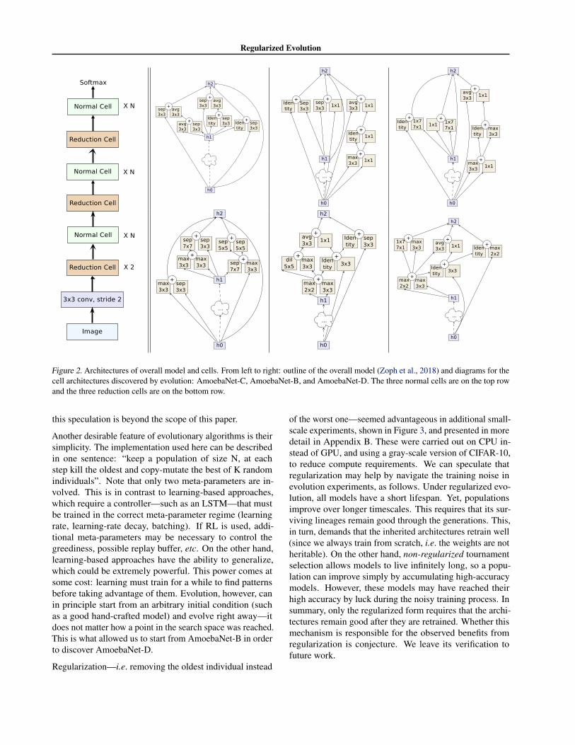
Figure 2. Architectures of overall model and cells. From left to right: outline of the overall model (Zoph et al., 2018) and diagrams for thecell architectures discovered by evolution: AmoebaNet-C, AmoebaNet-B, and AmoebaNet-D. The three normal cells are on the top rowand the three reduction cells are on the bottom row.

this speculation is beyond the scope of this paper.

Another desirable feature of evolutionary algorithms is theirsimplicity. The implementation used here can be describedin one sentence: “keep a population of size N, at eachstep kill the oldest and copy-mutate the best of K randomindividuals”. Note that only two meta-parameters are in-volved. This is in contrast to learning-based approaches,which require a controller—such as an LSTM—that mustbe trained in the correct meta-parameter regime (learningrate, learning-rate decay, batching). If RL is used, addi-tional meta-parameters may be necessary to control thegreediness, possible replay buffer, etc. On the other hand,learning-based approaches have the ability to generalize,which could be extremely powerful. This power comes atsome cost: learning must train for a while to find patternsbefore taking advantage of them. Evolution, however, canin principle start from an arbitrary initial condition (suchas a good hand-crafted model) and evolve right away—itdoes not matter how a point in the search space was reached.This is what allowed us to start from AmoebaNet-B in orderto discover AmoebaNet-D.

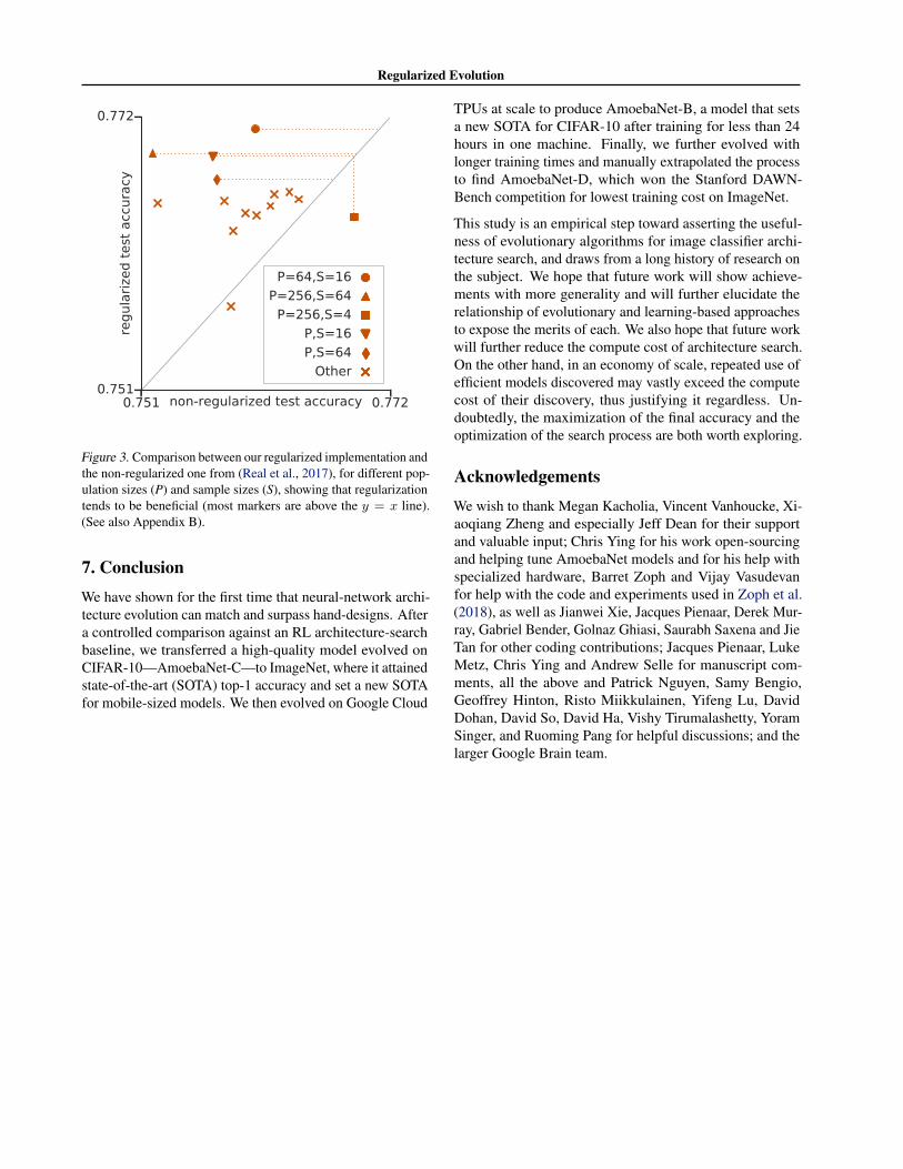
Regularization—i.e. removing the oldest individual instead

of the worst one—seemed advantageous in additional small-scale experiments, shown in Figure 3, and presented in moredetail in Appendix B. These were carried out on CPU in-stead of GPU, and using a gray-scale version of CIFAR-10,to reduce compute requirements. We can speculate thatregularization may help by navigate the training noise inevolution experiments, as follows. Under regularized evo-lution, all models have a short lifespan. Yet, populationsimprove over longer timescales. This requires that its sur-viving lineages remain good through the generations. This,in turn, demands that the inherited architectures retrain well(since we always train from scratch, i.e. the weights are notheritable). On the other hand, non-regularized tournamentselection allows models to live infinitely long, so a popu-lation can improve simply by accumulating high-accuracymodels. However, these models may have reached theirhigh accuracy by luck during the noisy training process. Insummary, only the regularized form requires that the archi-tectures remain good after they are retrained. Whether thismechanism is responsible for the observed benefits fromregularization is conjecture. We leave its verification tofuture work.

Regularized Evolution

0.751 0.772non-regularized test accuracy0.751

0.772re

gula

rize

d t

est

acc

ura

cy

P=64,S=16

P=256,S=64

P=256,S=4

P,S=16

P,S=64

Other

Figure 3. Comparison between our regularized implementation andthe non-regularized one from (Real et al., 2017), for different pop-ulation sizes (P) and sample sizes (S), showing that regularizationtends to be beneficial (most markers are above the y = x line).(See also Appendix B).

7. ConclusionWe have shown for the first time that neural-network archi-tecture evolution can match and surpass hand-designs. Aftera controlled comparison against an RL architecture-searchbaseline, we transferred a high-quality model evolved onCIFAR-10—AmoebaNet-C—to ImageNet, where it attainedstate-of-the-art (SOTA) top-1 accuracy and set a new SOTAfor mobile-sized models. We then evolved on Google Cloud

TPUs at scale to produce AmoebaNet-B, a model that setsa new SOTA for CIFAR-10 after training for less than 24hours in one machine. Finally, we further evolved withlonger training times and manually extrapolated the processto find AmoebaNet-D, which won the Stanford DAWN-Bench competition for lowest training cost on ImageNet.

This study is an empirical step toward asserting the useful-ness of evolutionary algorithms for image classifier archi-tecture search, and draws from a long history of research onthe subject. We hope that future work will show achieve-ments with more generality and will further elucidate therelationship of evolutionary and learning-based approachesto expose the merits of each. We also hope that future workwill further reduce the compute cost of architecture search.On the other hand, in an economy of scale, repeated use ofefficient models discovered may vastly exceed the computecost of their discovery, thus justifying it regardless. Un-doubtedly, the maximization of the final accuracy and theoptimization of the search process are both worth exploring.

AcknowledgementsWe wish to thank Megan Kacholia, Vincent Vanhoucke, Xi-aoqiang Zheng and especially Jeff Dean for their supportand valuable input; Chris Ying for his work open-sourcingand helping tune AmoebaNet models and for his help withspecialized hardware, Barret Zoph and Vijay Vasudevanfor help with the code and experiments used in Zoph et al.(2018), as well as Jianwei Xie, Jacques Pienaar, Derek Mur-ray, Gabriel Bender, Golnaz Ghiasi, Saurabh Saxena and JieTan for other coding contributions; Jacques Pienaar, LukeMetz, Chris Ying and Andrew Selle for manuscript com-ments, all the above and Patrick Nguyen, Samy Bengio,Geoffrey Hinton, Risto Miikkulainen, Yifeng Lu, DavidDohan, David So, David Ha, Vishy Tirumalashetty, YoramSinger, and Ruoming Pang for helpful discussions; and thelarger Google Brain team.

Regularized Evolution

Appendix A: Evolution vs. Reinforcement Learning

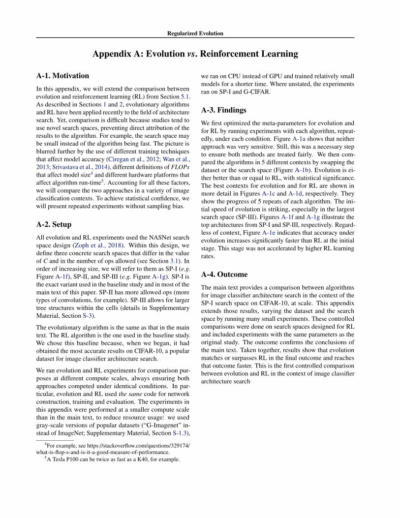
A-1. MotivationIn this appendix, we will extend the comparison betweenevolution and reinforcement learning (RL) from Section 5.1.As described in Sections 1 and 2, evolutionary algorithmsand RL have been applied recently to the field of architecturesearch. Yet, comparison is difficult because studies tend touse novel search spaces, preventing direct attribution of theresults to the algorithm. For example, the search space maybe small instead of the algorithm being fast. The picture isblurred further by the use of different training techniquesthat affect model accuracy (Ciregan et al., 2012; Wan et al.,2013; Srivastava et al., 2014), different definitions of FLOPsthat affect model size4 and different hardware platforms thataffect algorithm run-time5. Accounting for all these factors,we will compare the two approaches in a variety of imageclassification contexts. To achieve statistical confidence, wewill present repeated experiments without sampling bias.

A-2. SetupAll evolution and RL experiments used the NASNet searchspace design (Zoph et al., 2018). Within this design, wedefine three concrete search spaces that differ in the valueof C and in the number of ops allowed (see Section 3.1). Inorder of increasing size, we will refer to them as SP-I (e.g.Figure A-1f), SP-II, and SP-III (e.g. Figure A-1g). SP-I isthe exact variant used in the baseline study and in most of themain text of this paper. SP-II has more allowed ops (moretypes of convolutions, for example). SP-III allows for largertree structures within the cells (details in SupplementaryMaterial, Section S-3).

The evolutionary algorithm is the same as that in the maintext. The RL algorithm is the one used in the baseline study.We chose this baseline because, when we began, it hadobtained the most accurate results on CIFAR-10, a populardataset for image classifier architecture search.

We ran evolution and RL experiments for comparison pur-poses at different compute scales, always ensuring bothapproaches competed under identical conditions. In par-ticular, evolution and RL used the same code for networkconstruction, training and evaluation. The experiments inthis appendix were performed at a smaller compute scalethan in the main text, to reduce resource usage: we usedgray-scale versions of popular datasets (“G-Imagenet” in-stead of ImageNet; Supplementary Material, Section S-1.3),

4For example, see https://stackoverflow.com/questions/329174/what-is-flop-s-and-is-it-a-good-measure-of-performance.

5A Tesla P100 can be twice as fast as a K40, for example.

we ran on CPU instead of GPU and trained relatively smallmodels for a shorter time. Where unstated, the experimentsran on SP-I and G-CIFAR.

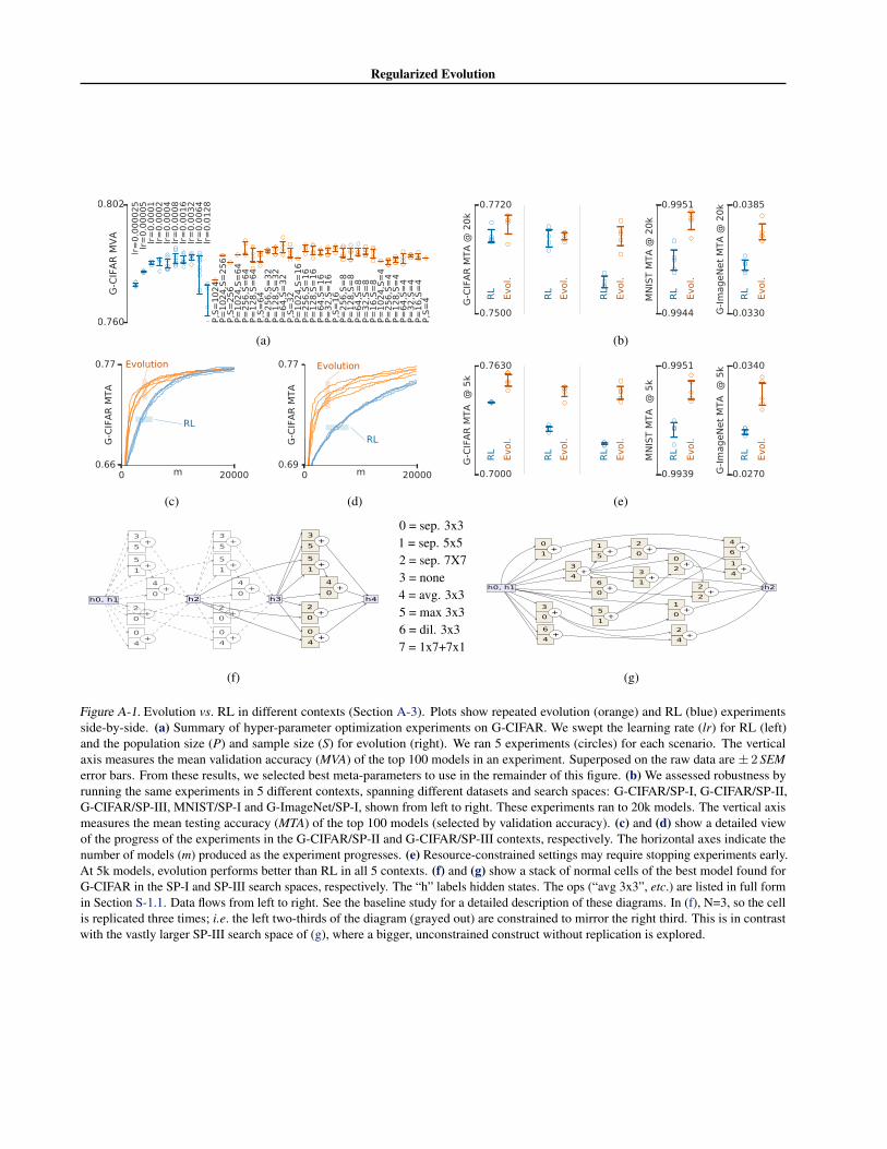
A-3. FindingsWe first optimized the meta-parameters for evolution andfor RL by running experiments with each algorithm, repeat-edly, under each condition. Figure A-1a shows that neitherapproach was very sensitive. Still, this was a necessary stepto ensure both methods are treated fairly. We then com-pared the algorithms in 5 different contexts by swapping thedataset or the search space (Figure A-1b). Evolution is ei-ther better than or equal to RL, with statistical significance.The best contexts for evolution and for RL are shown inmore detail in Figures A-1c and A-1d, respectively. Theyshow the progress of 5 repeats of each algorithm. The ini-tial speed of evolution is striking, especially in the largestsearch space (SP-III). Figures A-1f and A-1g illustrate thetop architectures from SP-I and SP-III, respectively. Regard-less of context, Figure A-1e indicates that accuracy underevolution increases significantly faster than RL at the initialstage. This stage was not accelerated by higher RL learningrates.

A-4. OutcomeThe main text provides a comparison between algorithmsfor image classifier architecture search in the context of theSP-I search space on CIFAR-10, at scale. This appendixextends those results, varying the dataset and the searchspace by running many small experiments. These controlledcomparisons were done on search spaces designed for RLand included experiments with the same parameters as theoriginal study. The outcome confirms the conclusions ofthe main text. Taken together, results show that evolutionmatches or surpasses RL in the final outcome and reachesthat outcome faster. This is the first controlled comparisonbetween evolution and RL in the context of image classifierarchitecture search

Regularized Evolution

lr=

0.0

00

02

5lr

=0

.00

00

5lr

=0

.00

01

lr=

0.0

00

2lr

=0

.00

04

lr=

0.0

00

8lr

=0

.00

16

lr=

0.0

03

2lr

=0

.00

64

lr=

0.0

12

8

0.760

0.802

G-C

IFA

R M

VA

P,S

=1

02

4P=

10

24

,S=

25

6P,S

=2

56

P=

10

24

,S=

64

P=

25

6,S

=6

4P=

12

8,S

=6

4P,S

=6

4P=

25

6,S

=3

2P=

12

8,S

=3

2P=

64

,S=

32

P,S

=3

2P=

10

24

,S=

16

P=

25

6,S

=1

6P=

12

8,S

=1

6P=

64

,S=

16

P=

32

,S=

16

P,S

=1

6P=

25

6,S

=8

P=

12

8,S

=8

P=

64

,S=

8P=

32

,S=

8P=

16

,S=

8P=

10

24

,S=

4P=

25

6,S

=4

P=

12

8,S

=4

P=

64

,S=

4P=

32

,S=

4P=

16

,S=

4P,S

=4

(a)

RL

Evol.

0.7500

0.7720

G-C

IFA

R M

TA

@ 2

0k

RL

Evol.

RL

Evol.

RL

Evol.

0.9944

0.9951

MN

IST M

TA

@ 2

0k

RL

Evol.

0.0330

0.0385

G-I

mageN

et

MTA

@ 2

0k

(b)

0 20000m0.66

0.77

G-C

IFA

R M

TA

Evolution

RL

(c)

0 20000m0.69

0.77

G-C

IFA

R M

TA

Evolution

RL

(d)R

L

Evol.

0.7000

0.7630

G-C

IFA

R M

TA

@

5k

RL

Evol.

RL

Evol.

RL

Evol.

0.9939

0.9951

MN

IST M

TA

@

5k

RL

Evol.

0.0270

0.0340

G-I

mageN

et

MTA

@

5k

(e)

(f)

0 = sep. 3x31 = sep. 5x52 = sep. 7X73 = none4 = avg. 3x35 = max 3x36 = dil. 3x37 = 1x7+7x1

(g)

Figure A-1. Evolution vs. RL in different contexts (Section A-3). Plots show repeated evolution (orange) and RL (blue) experimentsside-by-side. (a) Summary of hyper-parameter optimization experiments on G-CIFAR. We swept the learning rate (lr) for RL (left)and the population size (P) and sample size (S) for evolution (right). We ran 5 experiments (circles) for each scenario. The verticalaxis measures the mean validation accuracy (MVA) of the top 100 models in an experiment. Superposed on the raw data are ± 2 SEMerror bars. From these results, we selected best meta-parameters to use in the remainder of this figure. (b) We assessed robustness byrunning the same experiments in 5 different contexts, spanning different datasets and search spaces: G-CIFAR/SP-I, G-CIFAR/SP-II,G-CIFAR/SP-III, MNIST/SP-I and G-ImageNet/SP-I, shown from left to right. These experiments ran to 20k models. The vertical axismeasures the mean testing accuracy (MTA) of the top 100 models (selected by validation accuracy). (c) and (d) show a detailed viewof the progress of the experiments in the G-CIFAR/SP-II and G-CIFAR/SP-III contexts, respectively. The horizontal axes indicate thenumber of models (m) produced as the experiment progresses. (e) Resource-constrained settings may require stopping experiments early.At 5k models, evolution performs better than RL in all 5 contexts. (f) and (g) show a stack of normal cells of the best model found forG-CIFAR in the SP-I and SP-III search spaces, respectively. The “h” labels hidden states. The ops (“avg 3x3”, etc.) are listed in full formin Section S-1.1. Data flows from left to right. See the baseline study for a detailed description of these diagrams. In (f), N=3, so the cellis replicated three times; i.e. the left two-thirds of the diagram (grayed out) are constrained to mirror the right third. This is in contrastwith the vastly larger SP-III search space of (g), where a bigger, unconstrained construct without replication is explored.

Regularized Evolution

Appendix B: Regularized vs. Non-regularized Evolution

B-1. MotivationIn this appendix, we will extend the comparison betweenregularized evolution (RE) and non-regularized evolution(NRE) from Figure 3. As was described in Section 3.2,the evolutionary algorithm used in this paper keeps thepopulation size constant by always removing the oldestindividual whenever a new individual is added; we willrefer to this algorithm as RE. A recent paper used a similarmethod but kept the population size constant by removingthe worst individual in each tournament (Real et al., 2017);we will refer to that algorithm as NRE. This appendix willshow how these two algorithms compare in a variety ofcontexts.

B-2. SetupThe search spaces and datasets were the same as in Ap-pendix A, Section A-2.

B-3. Findings

NR

E

RE

0.7500

0.7730

G-C

IFA

R M

TA

@ 2

0k

NR

E

RE

RE

NR

E

NR

E

RE

0.9944

0.9951

MN

IST M

TA

@ 2

0k

NR

E

RE

0.0320

0.0422

G-I

mageN

et

MTA

@ 2

0k

Figure B-1. A comparison of NRE and RE under 5 differentcontexts, spanning different datasets and search spaces: G-CIFAR/SP-I, G-CIFAR/SP-II, G-CIFAR/SP-III, MNIST/SP-I andG-ImageNet/SP-I, shown from left to right. For each context,we show the final MTA of a few NRE and a few RE experiments(circles) in adjacent columns. We superpose ± 2 SEM error bars,where SEM denotes the standard error of the mean. The first con-text contains many repeats with identical meta-parameters andtheir MTA values seem normally distributed (Shapiro–Wilks test).Under this normality assumption, the error bars represent 95%confidence intervals.

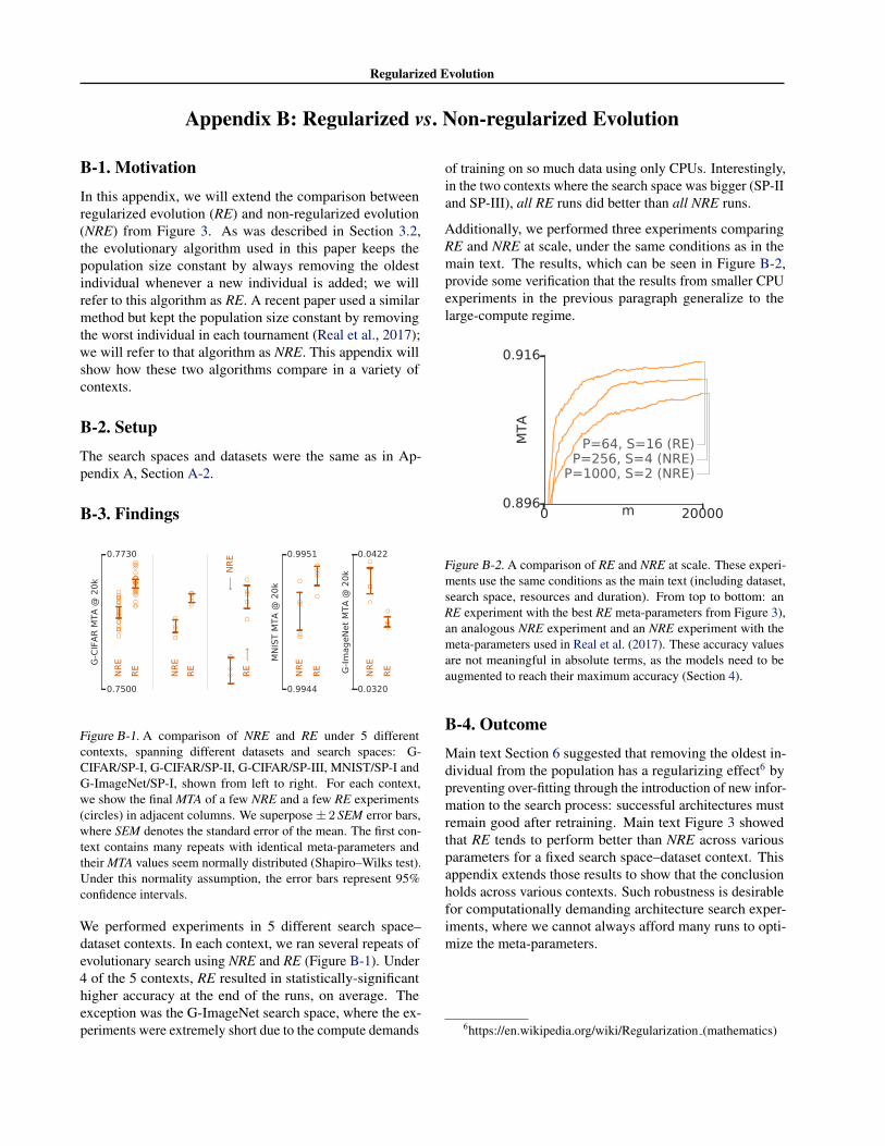
We performed experiments in 5 different search space–dataset contexts. In each context, we ran several repeats ofevolutionary search using NRE and RE (Figure B-1). Under4 of the 5 contexts, RE resulted in statistically-significanthigher accuracy at the end of the runs, on average. Theexception was the G-ImageNet search space, where the ex-periments were extremely short due to the compute demands

of training on so much data using only CPUs. Interestingly,in the two contexts where the search space was bigger (SP-IIand SP-III), all RE runs did better than all NRE runs.

Additionally, we performed three experiments comparingRE and NRE at scale, under the same conditions as in themain text. The results, which can be seen in Figure B-2,provide some verification that the results from smaller CPUexperiments in the previous paragraph generalize to thelarge-compute regime.

0 20000m0.896

0.916

MTA

P=64, S=16 (RE)P=256, S=4 (NRE)

P=1000, S=2 (NRE)

Figure B-2. A comparison of RE and NRE at scale. These experi-ments use the same conditions as the main text (including dataset,search space, resources and duration). From top to bottom: anRE experiment with the best RE meta-parameters from Figure 3),an analogous NRE experiment and an NRE experiment with themeta-parameters used in Real et al. (2017). These accuracy valuesare not meaningful in absolute terms, as the models need to beaugmented to reach their maximum accuracy (Section 4).

B-4. OutcomeMain text Section 6 suggested that removing the oldest in-dividual from the population has a regularizing effect6 bypreventing over-fitting through the introduction of new infor-mation to the search process: successful architectures mustremain good after retraining. Main text Figure 3 showedthat RE tends to perform better than NRE across variousparameters for a fixed search space–dataset context. Thisappendix extends those results to show that the conclusionholds across various contexts. Such robustness is desirablefor computationally demanding architecture search exper-iments, where we cannot always afford many runs to opti-mize the meta-parameters.

6https://en.wikipedia.org/wiki/Regularization (mathematics)

Regularized Evolution

References

Andrychowicz, Marcin, Denil, Misha, Gomez, Sergio, Hoff-man, Matthew W, Pfau, David, Schaul, Tom, and de Fre-itas, Nando. Learning to learn by gradient descent bygradient descent. In Advances in Neural InformationProcessing Systems, pp. 3981–3989, 2016.

Angeline, Peter J, Saunders, Gregory M, and Pollack, Jor-dan B. An evolutionary algorithm that constructs re-current neural networks. IEEE transactions on NeuralNetworks, 5(1):54–65, 1994.

Baker, Bowen, Gupta, Otkrist, Naik, Nikhil, and Raskar,Ramesh. Designing neural network architectures usingreinforcement learning. In International Conference onLearning Representations, 2017a.

Baker, Bowen, Gupta, Otkrist, Raskar, Ramesh, and Naik,Nikhil. Accelerating neural architecture search usingperformance prediction. International Conference onLearning Representations, Workshop Track, 2017b.

Bergstra, James and Bengio, Yoshua. Random search forhyper-parameter optimization. Journal of Machine Learn-ing Research, 13(Feb):281–305, 2012.

Brock, Andrew, Lim, Theodore, Ritchie, James M, andWeston, Nick. Smash: one-shot model architecture searchthrough hypernetworks. In International Conference onLearning Representations, 2018.

Cai, Han, Chen, Tianyao, Zhang, Weinan, Yu, Yong, andWang, Jun. Efficient architecture search by network trans-formation. In AAAI Conference on Artificial Intelligence,2018.

Chatfield, Ken, Simonyan, Karen, Vedaldi, Andrea, andZisserman, Andrew. Return of the devil in the details:Delving deep into convolutional nets. British MachineVision Conference, 2014.

Chen, Yunpeng, Li, Jianan, Xiao, Huaxin, Jin, Xiaojie, Yan,Shuicheng, and Feng, Jiashi. Dual path networks. InAdvances in Neural Information Processing Systems, pp.4470–4478, 2017.

Chollet, Francois. Xception: Deep learning with depthwiseseparable convolutions. Conference on Computer Visionand Pattern Recognition, 2017.

Ciregan, Dan, Meier, Ueli, and Schmidhuber, Jurgen. Multi-column deep neural networks for image classification.In IEEE Conference on Computer Vision and PatternRecognition, pp. 3642–3649. IEEE, 2012.

Coleman, Cody, Narayanan, Deepak, Kang, Daniel, Zhao,Tian, Zhang, Jian, Nardi, Luigi, Bailis, Peter, Olukotun,Kunle, Re, Chris, and Zaharia, Matei. Dawnbench: Anend-to-end deep learning benchmark and competition.Training, 100(101):102, 2017.

Cortes, Corinna, Gonzalvo, Xavi, Kuznetsov, Vitaly, Mohri,Mehryar, and Yang, Scott. Adanet: Adaptive structurallearning of artificial neural networks. In InternationalConference on Machine Learning, 2017.

Cubuk, Ekin D, Zoph, Barret, Mane, Dandelion, Vasude-van, Vijay, and Le, Quoc V. Autoaugment: Learn-ing augmentation policies from data. arXiv preprintarXiv:1805.09501, 2018.

Deng, Jia, Dong, Wei, Socher, Richard, Li, Li-Jia, Li, Kai,and Fei-Fei, Li. Imagenet: A large-scale hierarchicalimage database. In IEEE Conference on Computer Visionand Pattern Recognition, 2009.

DeVries, Terrance and Taylor, Graham W. Improved regu-larization of convolutional neural networks with cutout.arXiv preprint arXiv:1708.04552, 2017.

Domhan, Tobias, Springenberg, Jost Tobias, and Hutter,Frank. Speeding up automatic hyperparameter optimiza-tion of deep neural networks by extrapolation of learningcurves. In Proceedings of the Twenty-Fourth Interna-tional Joint Conference on Artificial Intelligence, 2017.

Donahue, Jeffrey, Anne Hendricks, Lisa, Guadarrama,Sergio, Rohrbach, Marcus, Venugopalan, Subhashini,Saenko, Kate, and Darrell, Trevor. Long-term recur-rent convolutional networks for visual recognition anddescription. In Proceedings of the IEEE conference oncomputer vision and pattern recognition, pp. 2625–2634,2015.

Dong, Jin-Dong, Cheng, An-Chieh, Juan, Da-Cheng, Wei,Wei, and Sun, Min. Ppp-net: Platform-aware progressivesearch for pareto-optimal neural architectures. Interna-tional Conference on Learning Representations, Work-shop Track, 2018.

Elsken, Thomas, Metzen, Jan-Hendrik, and Hutter, Frank.Simple and efficient architecture search for convolutionalneural networks. International Conference on LearningRepresentations, Workshop Track, 2017.

Fahlman, Scott E and Lebiere, Christian. The cascade-correlation learning architecture. In Advances in NeuralInformation Processing Systems, pp. 524–532, 1990.

Regularized Evolution

Fernando, Chrisantha, Banarse, Dylan, Reynolds, Malcolm,Besse, Frederic, Pfau, David, Jaderberg, Max, Lanctot,Marc, and Wierstra, Daan. Convolution by evolution:Differentiable pattern producing networks. In GECCO,pp. 109–116. ACM, 2016.

Fernando, Chrisantha, Banarse, Dylan, Blundell, Charles,Zwols, Yori, Ha, David, Rusu, Andrei A, Pritzel, Alexan-der, and Wierstra, Daan. Pathnet: Evolution channelsgradient descent in super neural networks. arXiv preprintarXiv:1701.08734, 2017.

Feurer, Matthias, Klein, Aaron, Eggensperger, Katharina,Springenberg, Jost, Blum, Manuel, and Hutter, Frank.Efficient and robust automated machine learning. In Ad-vances in Neural Information Processing Systems, 2015.

Floreano, Dario, Durr, Peter, and Mattiussi, Claudio. Neu-roevolution: from architectures to learning. EvolutionaryIntelligence, 1(1):47–62, 2008.

Gastaldi, Xavier. Shake-shake regularization. Interna-tional Conference on Learning Representations, Work-shop Track, and arXiv preprint arXiv:1705.07485, 2017.

Goldberg, David E and Deb, Kalyanmoy. A comparativeanalysis of selection schemes used in genetic algorithms.Foundations of genetic algorithms, 1:69–93, 1991.

Han, Dongyoon, Kim, Jiwhan, and Kim, Junmo. Deeppyramidal residual networks. In IEEE Conference onComputer Vision and Pattern Recognition, 2016.

He, Kaiming, Zhang, Xiangyu, Ren, Shaoqing, and Sun,Jian. Spatial pyramid pooling in deep convolutional net-works for visual recognition. In european conference oncomputer vision, pp. 346–361. Springer, 2014.

He, Kaiming, Zhang, Xiangyu, Ren, Shaoqing, and Sun,Jian. Deep residual learning for image recognition. InIEEE Conference on Computer Vision and Pattern Recog-nition, 2016.

Howard, Andrew G, Zhu, Menglong, Chen, Bo,Kalenichenko, Dmitry, Wang, Weijun, Weyand, Tobias,Andreetto, Marco, and Adam, Hartwig. Mobilenets: Ef-ficient convolutional neural networks for mobile visionapplications. arXiv preprint arXiv:1704.04861, 2017.

Hu, Jie, Shen, Li, and Sun, Gang. Squeeze-and-excitationnetworks. IEEE Conference on Computer Vision andPattern Recognition, 2018.

Huang, Furong, Ash, Jordan, Langford, John, and Schapire,Robert. Learning deep resnet blocks sequentially usingboosting theory. Advances on Neural Information Pro-cessing Systems, 2017a.

Huang, Gao, Liu, Zhuang, Weinberger, Kilian Q, andvan der Maaten, Laurens. Densely connected convolu-tional networks. In IEEE Conference on Computer Visionand Pattern Recognition, 2017b.

Jaderberg, Max, Simonyan, Karen, Zisserman, Andrew, et al.Spatial transformer networks. In Advances in neuralinformation processing systems, pp. 2017–2025, 2015.

Jaderberg, Max, Dalibard, Valentin, Osindero, Simon, Czar-necki, Wojciech M, Donahue, Jeff, Razavi, Ali, Vinyals,Oriol, Green, Tim, Dunning, Iain, Simonyan, Karen, et al.Population based training of neural networks. arXivpreprint arXiv:1711.09846, 2017.

Karpathy, Andrej, Toderici, George, Shetty, Sanketh, Leung,Thomas, Sukthankar, Rahul, and Fei-Fei, Li. Large-scalevideo classification with convolutional neural networks.In Proceedings of the IEEE conference on ComputerVision and Pattern Recognition, pp. 1725–1732, 2014.

Klein, Aaron, Falkner, Stefan, Springenberg, Jost Tobias,and Hutter, Frank. Learning curve prediction withbayesian neural networks. International Conference onLearning Representations, 2017.

Krizhevsky, Alex and Hinton, Geoffrey. Learning multiplelayers of features from tiny images. Master’s thesis, Dept.of Computer Science, U. of Toronto, 2009.

Krizhevsky, Alex, Sutskever, Ilya, and Hinton, Geoffrey E.Imagenet classification with deep convolutional neuralnetworks. In Advances in Neural Information ProcessingSystems, 2012.

Larsson, Gustav, Maire, Michael, and Shakhnarovich, Gre-gory. Fractalnet: Ultra-deep neural networks withoutresiduals. International Conference on Learning Repre-sentations, 2017.

Lin, Min, Chen, Qiang, and Yan, Shuicheng. Network innetwork. International Conference on Learning Repre-sentations, 2014.

Liu, Chenxi, Zoph, Barret, Shlens, Jonathon, Hua, Wei, Li,Li-Jia, Fei-Fei, Li, Yuille, Alan, Huang, Jonathan, andMurphy, Kevin. Progressive neural architecture search.arXiv preprint arXiv:1712.00559, 2017.

Liu, Hanxiao, Simonyan, Karen, Vinyals, Oriol, Fernando,Chrisantha, and Kavukcuoglu, Koray. Hierarchical rep-resentations for efficient architecture search. In Interna-tional Conference on Learning Representations, 2018.

Mendoza, Hector, Klein, Aaron, Feurer, Matthias, Sprin-genberg, Jost Tobias, and Hutter, Frank. Towardsautomatically-tuned neural networks. In Workshop onAutomatic Machine Learning, 2016.

Regularized Evolution

Miikkulainen, Risto, Liang, Jason, Meyerson, Elliot,Rawal, Aditya, Fink, Dan, Francon, Olivier, Raju,Bala, Navruzyan, Arshak, Duffy, Nigel, and Hodjat,Babak. Evolving deep neural networks. arXiv preprintarXiv:1703.00548, 2017.

Negrinho, Renato and Gordon, Geoff. Deeparchitect: Auto-matically designing and training deep architectures. arXivpreprint arXiv:1704.08792, 2017.

Pham, Hieu, Guan, Melody Y., Zoph, Barret, Le, Quoc V.,and Dean, Jeff. Faster discovery of neural architectures bysearching for paths in a large model. International Con-ference on Learning Representations, Workshop Track,2018.

Real, Esteban, Moore, Sherry, Selle, Andrew, Saxena,Saurabh, Suematsu, Yutaka Leon, Le, Quoc, and Ku-rakin, Alex. Large-scale evolution of image classifiers.In International Conference on Machine Learning, 2017.

Sandler, Mark, Howard, Andrew, Zhu, Menglong, Zh-moginov, Andrey, and Chen, Liang-Chieh. Invertedresiduals and linear bottlenecks: [...]. arXiv preprintarXiv:1801.04381, 2018.

Saxena, Shreyas and Verbeek, Jakob. Convolutional neuralfabrics. In Advances in Neural Information ProcessingSystems, 2016.

Sermanet, Pierre, Eigen, David, Zhang, Xiang, Mathieu,Michael, Fergus, Rob, and LeCun, Yann. Overfeat: Inte-grated recognition, localization and detection using con-volutional networks. International Conference on Learn-ing Representations, 2014.

Simmons, Joseph P, Nelson, Leif D, and Simonsohn, Uri.False-positive psychology: Undisclosed flexibility in datacollection and analysis allows presenting anything assignificant. Psychological Science, 22(11):1359–1366,2011.

Simonyan, Karen and Zisserman, Andrew. Very deep con-volutional networks for large-scale image recognition.International Conference on Learning Representations,2015.

Srivastava, Nitish, Hinton, Geoffrey, Krizhevsky, Alex,Sutskever, Ilya, and Salakhutdinov, Ruslan. Dropout:A simple way to prevent neural networks from overfit-ting. The Journal of Machine Learning Research, 15(1):1929–1958, 2014.

Stanley, Kenneth O and Miikkulainen, Risto. Evolvingneural networks through augmenting topologies. Evolu-tionary Computation, 10(2):99–127, 2002.

Stanley, Kenneth O, D’Ambrosio, David B, and Gauci, Ja-son. A hypercube-based encoding for evolving large-scaleneural networks. Artificial life, 15(2):185–212, 2009.

Such, Felipe Petroski, Madhavan, Vashisht, Conti, Edoardo,Lehman, Joel, Stanley, Kenneth O, and Clune, Jeff. Deepneuroevolution: Genetic algorithms [...]. arXiv preprintarXiv:1712.06567, 2017.

Suganuma, Masanori, Shirakawa, Shinichi, and Nagao, To-moharu. A genetic programming approach to designingconvolutional neural network architectures. In Proceed-ings of the Genetic and Evolutionary Computation Con-ference, 2017.

Szegedy, Christian, Liu, Wei, Jia, Yangqing, Sermanet,Pierre, Reed, Scott, Anguelov, Dragomir, Erhan, Dumitru,Vanhoucke, Vincent, and Rabinovich, Andrew. Goingdeeper with convolutions. In IEEE Conference on Com-puter Vision and Pattern Recognition, 2015.

Szegedy, Christian, Vanhoucke, Vincent, Ioffe, Sergey,Shlens, Jon, and Wojna, Zbigniew. Rethinking the incep-tion architecture for computer vision. In IEEE Conferenceon Computer Vision and Pattern Recognition, 2016.

Szegedy, Christian, Ioffe, Sergey, Vanhoucke, Vincent, andAlemi, Alexander A. Inception-v4, inception-resnet andthe impact of residual connections on learning. In AAAIConference on Artificial Intelligence, volume 4, pp. 12,2017.

Wan, Li, Zeiler, Matthew, Zhang, Sixin, Le Cun, Yann, andFergus, Rob. Regularization of neural networks usingdropconnect. In International Conference on MachineLearning, pp. 1058–1066, 2013.

Xie, Lingxi and Yuille, Alan. Genetic CNN. In InternationalConference on Computer Vision, 2017.

Xie, Saining, Girshick, Ross, Dollar, Piotr, Tu, Zhuowen,and He, Kaiming. Aggregated residual transformationsfor deep neural networks. In IEEE Conference on Com-puter Vision and Pattern Recognition, 2017.

Yamada, Yoshihiro, Iwamura, Masakazu, and Kise, Koichi.Shakedrop regularization. International Conference onLearning Representations, Workshop Track, 2018.

Zagoruyko, Sergey and Komodakis, Nikos. Wide residualnetworks. In British Machine Vision Conference, 2016.

Zhang, Xiangyu, Zhou, Xinyu, Lin, Mengxiao, and Sun,Jian. Shufflenet: An extremely efficient convolutionalneural network for mobile devices. arXiv preprintarXiv:1707.01083, 2017a.

Regularized Evolution

Zhang, Xingcheng, Li, Zhizhong, Loy, Chen Change, andLin, Dahua. Polynet: A pursuit of structural diversityin very deep networks. In 2017 IEEE Conference onComputer Vision and Pattern Recognition (CVPR), pp.3900–3908. IEEE, 2017b.

Zhong, Zhao, Yan, Junjie, and Liu, Cheng-Lin. Practical net-work blocks design with q-learning. In AAAI Conferenceon Artificial Intelligence, 2018.

Zoph, Barret and Le, Quoc V. Neural architecture searchwith reinforcement learning. In International Conferenceon Learning Representations, 2016.

Zoph, Barret, Vasudevan, Vijay, Shlens, Jonathon, and Le,Quoc V. Learning transferable architectures for scalableimage recognition. In IEEE Conference on ComputerVision and Pattern Recognition, 2018.

Regularized Evolution

Supplementary Material

S-1. Detailed MethodsS-1.1. Search Space Details

Section 3.1 introduced the search space in outline. In thelanguage presented in Section 3, the space uses C = 5 and8 possible ops (identity; 3x3, 5x5 and 7x7 separable (sep.)convolutions (convs.); 3x3 average (avg.) pool; 3x3 maxpool; 3x3 dilated (dil.) sep. conv.; 1x7 then 7x1 conv.). Tofind AmoebaNet-B, 19 possible ops were allowed (identity;1x1 and 3x3 convs.; 3x3, 5x5 and 7x7 sep. convs.; 2x2 and3x3 avg. pools; 2x2 min pool.; 2x2 and 3x3 max pools; 3x3,5x5 and 7x7 dil. sep. convs.; 1x3 then 3x1 conv.; 1x7 then7x1 conv. 3x3 dil. conv. with rates 2, 4 and 6).

S-1.2. Architecture Search Algorithm Details

For all three algorithms—evolution, reinforcement learning(RL) and random search (RS)—the initial models producedhave random architectures. That is, the initial models havecells that are constructed with uniformly random ops, whichdraw from uniformly random inputs, subject to the con-straint that no loops should be formed. For RS, all modelsare constructed this way throughout the entirety of the ex-periment.

S-1.3. Datasets

We used the following datasets:• CIFAR-10 (Krizhevsky & Hinton, 2009): dataset with

naturalistic images labeled with 1 of 10 common objectclasses. It has 50k training examples and 10k test exam-ples, all of which are 32 x 32 color images. 5k of thetraining examples were held out in a validation set. Theremaining 45k examples were used for training.

• G-CIFAR: a grayscaled version of CIFAR-10. The origi-nal images were each averaged across channels. Training,validation and testing set splits were preserved.

• MNIST: a handwritten black-and-white digit classifica-tion dataset. It has 60k and 10k testing examples. Weheld out 5k for validation. The labels are the digits 0-9.

• ImageNet (Deng et al., 2009): large set of naturalistic im-ages, each labeled with one or more objects from among1k classes. Contains a total of about 1.2M 331x331 exam-ples. Of these, 50k were held out for validation and therest constituted the training set. The standard validationset of 50k was used for testing.

• G-ImageNet: a grayscaled subset of ImageNet. The orig-inal images were averaged across channels and re-sizedto 32x32. We generated a training set with 200k randomimages from the standard training set. We also held out10k images from it for validation. The standard validation

set of 50k was used for testing.

S-1.4. Experiment Setup Details

The following completes the description of experiments inSection 4. Each experiment ended when 20k models weretrained. Each model trained for 25 epochs. C = 5, N = 3and F = 24. To compare different approaches, it was impor-tant that the results be independent of the hardware type andnetwork usage. To achieve such hardware-independence, afixed number of training-steps-per-model and a fixed num-ber of models-per-experiment were used, causing variabletraining times. Yet, the observed advantage of the evolu-tionary approach was not due to longer training times. Infact, the evolutionary approach ran faster experiments withshorter training times than RL—as may be guessed fromthe efficiency of the final models shown in Figure 1 (right).

Section 5.3 introduced a new setup for evolving on GoogleCloud TPUs. This was the same as those in Section 4, ex-cept that the models were larger (F = 32) and the trainingwas longer (50 epochs). By training larger models for moreepochs, the search phase validation accuracy is more rep-resentative of the true validation accuracy when the modelis scaled up in parameters, i.e. a model evaluated with(N = 3, F = 32, 50 epochs) is likely to be better than(N = 3, F = 24, 25 epochs) at predicting performance of(N = 6, F = 32, 600 epochs). The experiment ran on 225Google Cloud TPUs for 5 days and trained 27k models total.Each TPU supported 4 workers.

S-1.5. Augmented Model Selection

To compare augmented models side-by-side (Figure 1,right), we selected from each evolution or RL experimentthe top 20 models by validation accuracy. We augmentedall of them equally by setting N = 6 and F = 32, as wasdone in the experiment that produced NASNet-A in the base-line study. Finally, we trained them on CIFAR-10 (detailsbelow).

To find AmoebaNet-C (Table 1), we selected the model withthe best tradeoff between complexity and CIFAR-10 testaccuracy among evolution models in Figure 1. Note thatusing test accuracy was reasonable because the architectureis selected for ImageNet transfer, and not for presentingresults on CIFAR-10 (the model used for the CIFAR-10table was selected by validation, as described in the nextparagraph).

To find AmoebaNet-B (Table 3), we selected K = 100models from the TPU experiment. To do this, we binned the

Regularized Evolution

models by their number of parameters to cover the range,using b bins. From each bin, we took the top K/b modelsby validation accuracy. We then augmented all models toN = 6 and F = 32 and picked the one with the highestvalidation accuracy. We then re-augmented this model withthe (N,F ) values in Table 3. Note that we report all 3sizes; as the size increases, the mean accuracy increases asexpected, so there is little risk of overfitting due to evaluating3 times (which is standard reporting methodology anyway).We trained each size 8 times on CIFAR-10 to measure themean testing accuracy. Using the mean (as opposed tothe maximum) ensures there is no overfitting from these 8repeats.

S-1.6. Augmented Model Training

To train augmented models on CIFAR-10, we followed sim-ilar training, data augmentation, and evaluation proceduresto those in (Zoph et al., 2018). We used one Google CloudTPUv2 with batch size 128, SGD with momentum optimizerand momentum rate set to 0.9, L2 weight regularization withrate 5x10−4, initial learning rate of 0.024 with cosine decayto zero over 600 epochs, and ScheduledDropPath (Zophet al., 2018) with a final keep-probability of 0.7. Duringtraining, the model used an auxiliary softmax classifier 2/3down the network weighted by 0.5. To report validationaccuracy, the held out validation was not included in thetraining. To report testing accuracy, the full training set wasused.

To train augmented models on ImageNet we adjusted thesize so that the number of trainable parameters in the modelis comparable to others from the literature. For mobile sizemodels, we used 224x224 input images and set the reductionsize F to 44 and 54—to compare against PNASNet-5 (N=3,F=54) and MobileNetV2 (1.4), respectively. For large-sizemodels, we used 331x331 input images and set the reduc-tion size F to 168 (to compare against PNASNet-5 N4F216)and to 228 (the biggest model supported by P100 GPUs).We followed similar training, data augmentation, and eval-uation procedures to those in (Szegedy et al., 2016). Weused distributed synchronous SGD with 100 P100 GPUs.We employed RMSProp optimizer with a decay of 0.9 andε = 0.1, L2 regularization with weight decay 4 × 10−5,label smoothing with value 0.1 and an auxiliary softmaxclassifier weighted by 0.4. We applied dropout to the finalsoftmax layer with probability 0.5. We apply Scheduled-DropPath (Zoph et al., 2018) with a final keep-probabilityof 0.7. That is, we randomly drop out each connectionedge in the cell architecture diagram with probability thatincreases linearly over the course of the training, reachingat the end a 0.7 chance that any edge will be kept. Thelearning rate started at 0.001 and decayed every 2 epochswith rate 0.97. Due to resource limitations, we applied thesame hyper-parameters to all models we reported in tables 1

and 2 without further hyper-parameter tuning.

Where possible, we report our model’s test error as µ± 2×SEM. This applies to the uncertainties in the tables and theerror bars in the figures. We report inference number ofparameters and FLOPs.

S-2. Baseline Comparison AddendaA comparison between two given algorithms will be biasedif the meta-parameters are not equally well optimized forboth. We took steps to ensure that the meta-parameters forRL were at least as optimized as those for evolution. Westarted with the meta-parameters from the baseline study(under identical conditions) and fine-tuned them by sweep-ing the lr until we saw the accuracy decline at both extremes.We tried: lr = 0.00003, lr = 0.00006, lr = 0.00012,lr = 0.0002, lr = 0.0004, lr = 0.0008, lr = 0.0016,lr = 0.0032. The best lr was 0.0008, which is the samevalue as that found in the smaller-scale experiments of Ap-pendix A.

In order to avoid selection bias, the experiment repeats plot-ted in Figure 1 do not include the actual runs from the op-timization stage described here. Only the meta-parametersfound carry over. This was a decision made a priori.

S-3. Supplementary Appendix MaterialSection A-2 performs experiments using 3 distinct searchspaces, SP-I, SP-II and SP-III, and described them in outline.In the language presented in Section 3, these can be definedas:• SP-I: the same space as in the main text, already defined

in Section S-1.1. See also Figure A-1f;• SP-II: uses C = 5 and 19 possible ops (identity; 1x1 and

3x3 convs.; 3x3, 5x5 and 7x7 sep. convs.; 2x2 and 3x3avg. pools; 2x2 min pool.; 2x2 and 3x3 max pools; 3x3,5x5 and 7x7 dil. sep. convs.; 1x3 then 3x1 conv.; 1x7then 7x1 conv. 3x3 dil. conv. with rates 2, 4 and 6), and

• SP-III: uses C = 15 and 8 possible ops (same as SP-I)—see Figure A-1g.

Each appendix experiment ended when 20k models weretrained (i.e. 20k sample complexity). Each model trainedfor 4, 4 or 1 epochs in either the G-CIFAR, MNIST or G-ImageNet datasets, respectively. In all cases, C = 5, N = 3and F = 8. These settings were chosen to be as close aspossible to the large-scale experiments below while runningreasonably fast on CPU. Each experiment used 450 CPUworkers and lasted 2–5 days.