Regular Paper Isoperformance: Analysis and Design of ...

Isoperformance: Analysisand Design of ComplexSystems with DesiredOutcomes*Olivier L. de Weck1, † and Marshall B. Jones2

1Engineering Systems Division, Department of Aeronautics & Astronautics, 77 Massachusetts Avenue, 33-410, Massachusetts Institute of Technology, Cambridge, MA 02139

2Behavioral Science Department, 500 University Drive, Room C1728, Pennsylvania State University, Hershey, PA 17033

ISOPERFORMANCE: ANALYSIS AND DESIGN OF COMPLEX SYSTEMS WITH DESIRED OUTCOMES

Received 27 October 2004; Accepted 17 October 2005, after one or more revisionsPublished online in Wiley InterScience (www.interscience.wiley.com). DOI 10.1002/sys.20043

ABSTRACT

The design of technical systems such as automobiles and spacecraft has traditionally focusedexclusively on performance maximization. Many organizations now realize that such anapproach must be balanced against competing objectives of cost, risk, and other criteria. Ifone is willing to give up some amount of performance relative to the best achievableperformance level, one introduces slack into system design. This slack can be invested increating better outcomes overall. One way to achieve this is to balance the requirementsamong contributing subsystems such that the number of active constraints is minimized, whilestill achieving the desired system performance. This paper introduces a methodology called“isoperformance” as a means of identifying and evaluating a performance-invariant set ofdesign solutions, which are efficient in terms of other criteria such as cost, risk, and lifecycleproperties. Isoperformance is an inverse design method that starts from a desired vector ofperformance requirements and works backwards to identify acceptable solutions in the

Regular Paper

*This work was partially supported by the NASA Goddard SpaceFlight Center under Contracts No. NAG5-6079 and No. NAG5-7839and by the Jet Propulsion Laboratory under Contract No. JPL 961123.

†Author to whom all correspondence should be addressed (e-mail:[email protected]).

Systems Engineering, Vol. 9, No. 1, 2006© 2006 Wiley Periodicals, Inc.

45

design space. To achieve this, gradient-based contour following is implemented as a multi-variable search algorithm that manipulates the null set of the Jacobian matrix. Use of themethod is illustrated with two examples from spacecraft design and human performance insports. © 2006 Wiley Periodicals, Inc. Syst Eng 9: 45–61, 2006

Key words: system design; isoperformance; multiobjective optimization; constraints; gradi-ent-based search; inverse design methods; sensitivity analysis

1. INTRODUCTION

Engineers have been traditionally conditioned to thinkin particular ways about the challenging task of systemdesign. First, emphasis has been historically placed onperformance maximization, which was evident in pro-jects such as Apollo (1962–1973), the development ofthe Concorde (1956–1976) or even current practices inFormula 1 race car design. Second, the dominant wayin which design is taught and practiced is in the modeof “forward analysis.” Choices in the design space suchas material selection, geometry specification or control-ler gain settings are evaluated in terms of their impacton system response and objectives such as range, speed,and more recently fuel consumption. If initial designchoices are unsatisfactory, engineers typically iterate ontheir designs until such quantities have been maximizedor minimized, subject to a number of other technicaland financial feasibility constraints. This modus oper-andi is facilitated by the fact that, with the possibleexception of buckling and other instability situations,each vector of choices, x, in the design space can usuallybe uniquely mapped to an expected outcome in theobjective space, x D J(x).

This paradigm has its roots in an era where systemperformance was the prime driver of competitivenessand superiority. This is particularly true for aerospaceengineering, which has only recently come to realizethat performance is not necessarily limited by physicalphenomena (e.g., transonic drag, atmospheric proper-ties in the stratosphere) alone, but that “pushing theperformance envelope” too hard can have detrimentalconsequences for other aspects of the system. We findthe following quote by Schrage et al. [1991] to beparticularly appropriate: “The experience of the 1960’shas shown that for military aircraft the cost of the finalincrement of performance usually is excessive in termsof other characteristics and that the overall system mustbe optimized, not just performance.”

A more natural mode of thought is not to strive forthe “best achievable” system performance, but accept-able performance that is “good enough,” depending oncontractually specified requirements, the state of com-petition in various market segments, and the need to

achieve desired robust functionality at the lowest pos-sible cost. In that case the desired performance levelsbecome known quantities that can serve as targets forsystem designers. This is the focus of so-called inversedesign methods, whose goal it is to find a set of solu-tions in the design space that satisfy a set of perform-ance targets in the objective space, J D x(J). The mainchallenge lies in the nonuniqueness of the problem.Since the number of design variables generally farexceeds the number of objectives, there might be many,often infinitely many design vectors, xi, that satisfy thevector of performance targets, Jreq. This, of course,assumes that none of the targets are utopian, i.e., thatthe targets are feasible based on physics and availabletechnologies (but not necessarily based on availableresources).

Isoperformance is a method that addresses this prob-lem by first obtaining a performance invariant set ofsystem design solutions and subsequently reducingthese to an efficient set, when evaluated against othercriteria such as cost and risk. Said more simply, it is aninverse design method that allows system designers toask: “What is the set of feasible designs, Xiso, thatsatisfies all performance targets within some tolerance,while optimizing other criteria such as cost and risk?”.

Let us consider a simple example from rocketry toillustrate this point. The primary performance of arocket is measured by the change in velocity, ∆v, that itcan achieve for a specified payload mass mp. The rocketequation by Tsiolkovsky [1903] states that

∆v = vf − vi = g ⋅ Isp ⋅ ln

mi

mf

, (1)

where vi is the initial velocity in m/s, vf is the finalvelocity, g is Earth’s mean gravitational acceleration atthe surface, g = 9.81 m/s2, Isp is the specific impulse ofthe propulsion system in seconds, mi is the initial mass,and mf is the final mass after engine cutoff. The initialmass can be written as

mi = ms + mf + mp = (1 + α)mf + mp, (2)

46 DE WECK AND JONES

where ms is the structural (empty) mass of the rocket,mf is the mass of fuel, and mp is the payload mass. Forsimplicity one can assume that α represents the struc-tural mass of the rocket as a fraction of total fuel mass.Typical values for α are on the order of 0.08–0.12. Thefinal mass—assuming all fuel is consumed—is simply

mf = ms + mp = αmf + mp. (3)

If we were to design a rocket for launching payloads tolow Earth orbit, a typical performance requirementwould be Jreq = ∆vreq = 9500 m/s. This requirementallows achieving orbital velocity while absorbing drag,gravity, and flight path turning losses during ascent. Inother words, satisfactory performance is defined asaccelerating a payload mass of say, mp = 5000 kg, bythe velocity increment, ∆vreq. If the actual performanceachieved is below this level, a payload would not reachor remain in orbit and the system would be useless. Onthe other hand, if the system significantly exceeds therequirement, it will achieve its purpose but be overdes-igned and, as a consequence, be heavier, more complex,and more costly than really needed. So, what is thefamily of feasible rocket designs that satisfies the re-quired performance level?

Isoperformance is a method for thinking through andsolving this problem. After specifying the requiredfunction and performance level, one must understand

which variables in the system the designer can changeindependently, and which ones are constrained by na-ture or man to be fixed constants. In the case of rocketdesign we may choose the Isp (by selecting a particularoxidizer/propellant combination) and size of the rocket(by deciding on the quantity of fuel). Of course, archi-tectural decisions such as the number of rocket stagesmust be considered as well and we will return to thispoint later on. Let x = [x1 x2]T be the design vectorwith x1 = Isp and x2 = mf. The vector of fixed parametersis p = [p1 p2 p3]T with p1 = g = 9.81 m/s, p2 = mp = 5000kg, and p3 = α = 0.1.

Given the fact that we have n = 2 design variables inthis example, we can easily evaluate all possible designsbetween technologically feasible upper and lowerbounds:

x1, LB = 300 ≤ x1 ≤ x1, UB = 500,

x2, LB = 5 ⋅ 104 ≤ x2 ≤ x2, UB = 106. (4)

We can discretize this design space into small incre-ments, ∆xi, and evaluate all possible combinations ofspecific impulse and fuel mass. The result is shown inFigure 1 and depicts the characteristic “wall” caused bythe rocket equation. As Isp is decreased by a smallamount, it takes more and more propellant to achievethe same ∆v to make up for the loss of combustion

Figure 1. Isoperformance contours of v [km/s] for simple rocket example.

ISOPERFORMANCE: ANALYSIS AND DESIGN OF COMPLEX SYSTEMS WITH DESIRED OUTCOMES 47

efficiency. The plot shows the isoperformance contourof interest (9.5 km/s) and the relationship that must bemaintained between the design variables x1 and x2 tostay on the contour. Thus, there are an infinite numberof choices between the two extreme designs: A and B.A uses propulsion technology which is easily achiev-able, while B assumes an Isp of 500 s, which is verydifficult to achieve even with state-of-the-art liquid-hy-drogen, liquid-oxygen propulsion technology. Saidmore plainly, design A makes the job of the propulsionsubsystem designers easy but requires a very largerocket which creates structural and controls challenges.Design B, on the other hand, is small and compact, butvery challenging from a propulsion technology stand-point. It is interesting to note where various existingrocket stage designs fall in that space. The second stageof the Saturn V launch vehicle (Saturn5.2) falls exactlyonto the isoperformance contour and represents a com-promise design (close to design C) that meets perform-ance requirements but balances the difficulty betweenstructural and propulsion subsystems.1 Other systemssuch as the Space Shuttle second stage (STS.2), wouldbe significantly overdesigned or underdesigned (Atlas-I first stage), respectively.

This example, while accurate based on first princi-ples, does not capture some of the most importantconsiderations in selecting among designs A, B, or C.One example of such a secondary criterion is the timerequired to prepare the vehicle for launch. While oper-ating along the isoperformance contour (Fig. 1) may beefficient from a propulsion standpoint it implies thatcryogenic fluids will be used (LH2, LOX) and that arocket cannot be readied for launch with only a fewminutes notice. This is the main reason why designersof ICBMs chose lower Isp designs that could be readiedfor launch in minutes rather than hours. Acceptinglower propulsion performance was acceptable in thatcase because payloads were smaller and orbital veloci-ties did not have to be achieved due to ballistic reentry.

Finding the isoperformance contour in this examplewas trivial because we only considered two designvariables and a single objective. What if multiple objec-tives were to be considered together and the vector ofdesign variables were significantly larger? In that casefinding the set of isoperformance solutions is not trivial,and we must find ways to systematically search thedesign space for acceptable solutions. And, once suchsolutions are obtained, we must find means to reducethe large set of alternatives to a smaller set that can bepresented to decision-makers. Finally, criteria for se-

lecting a particular solution in the reduced set must bediscussed. These three sequential questions give rise tothe three steps of the isoperformance methodologypresented in this paper.

2. LITERATURE REVIEW AND PROBLEMFORMULATION

2.1. Related Literature

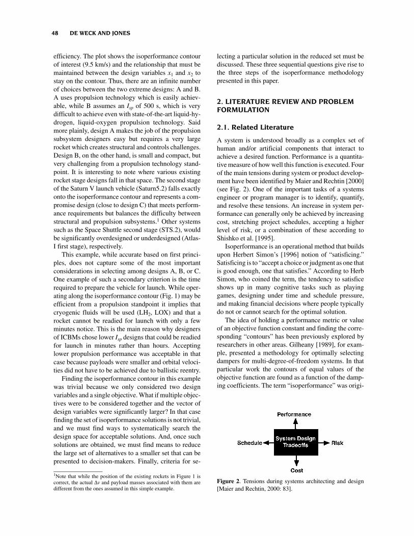
A system is understood broadly as a complex set ofhuman and/or artificial components that interact toachieve a desired function. Performance is a quantita-tive measure of how well this function is executed. Fourof the main tensions during system or product develop-ment have been identified by Maier and Rechtin [2000](see Fig. 2). One of the important tasks of a systemsengineer or program manager is to identify, quantify,and resolve these tensions. An increase in system per-formance can generally only be achieved by increasingcost, stretching project schedules, accepting a higherlevel of risk, or a combination of these according toShishko et al. [1995].

Isoperformance is an operational method that buildsupon Herbert Simon’s [1996] notion of “satisficing.”Satisficing is to “accept a choice or judgment as one thatis good enough, one that satisfies.” According to HerbSimon, who coined the term, the tendency to satisficeshows up in many cognitive tasks such as playinggames, designing under time and schedule pressure,and making financial decisions where people typicallydo not or cannot search for the optimal solution.

The idea of holding a performance metric or valueof an objective function constant and finding the corre-sponding “contours” has been previously explored byresearchers in other areas. Gilheany [1989], for exam-ple, presented a methodology for optimally selectingdampers for multi-degree-of-freedom systems. In thatparticular work the contours of equal values of theobjective function are found as a function of the damp-ing coefficients. The term “isoperformance” was origi-

1Note that while the position of the existing rockets in Figure 1 iscorrect, the actual ∆v and payload masses associated with them aredifferent from the ones assumed in this simple example.

Figure 2. Tensions during systems architecting and design[Maier and Rechtin, 2000: 83].


nally coined in the area of human factors research. Workhas been done by Kennedy, Jones, and coworkers [Ken-nedy, Turnage, and Jones, 1990; Jones and Kennedy,1996] on the need within the U.S. Department of De-fense to improve systems performance through betterintegration of men and women into military systems(human factors engineering). They present the applica-tion of isoperformance analysis in military and aero-space systems design, by trading off equipment,training variables, and user characteristics. Once thelevel of operational performance in these systems issettled upon (e.g., “pilot will check out all aircraftsystems within 30 seconds”), tradeoffs among equip-ment variables, adaptation, training, and individual pre-disposing factors can be made. Jones in particular hasalso linked isoperformance to personnel selection[2000].

Inverse design has recently become a topic in aero-dynamics where one would like to automatically gen-erate airfoil geometry (usually as a sequence of x/ycoordinates of control points) for a prescribed pressuredistribution over a wing (see, for example, Kim, Kim,and Rho [1999]). Level Set Methods in mathematicsalso have the potential to represent isoperformancesurfaces (see Osher and Fedkiw [2002]). So far, how-ever, these advanced geometrical techniques have beenmainly applied to visualization and computer graphics.

A number of researchers such as Taguchi, Cook[1997], and Messac [1996] have recognized that systemrequirements typically fall into one of three classes:“smaller-is-better” (SIB), “larger-is-better” (LIB), and“nominal-is-better” (NIB) (see Fig. 3). In automotivedesign, for example, a target average fuel economy[mpg] might have to be achieved (NIB) for a vehicle,while at the same time vehicle variable manufacturingcost [$] might have to be minimized (SIB) with interior

roominess [m3] being maximized (LIB). Which of theseobjectives are considered as NIB target values andwhich ones can be maximized or minimized dependson the particular circumstances. Typically, however,such objectives are counteracting. Large interior vol-ume would tend to increase drag, which in turn de-creases fuel economy. A target vehicle fuel economycan be achieved by trading off fuel capacity, emptyweight, and engine displacement among other vari-ables. The isoperformance approach assumes that de-sired performance targets Jreq are known, i.e., that thekey performance objectives are captured as NIB andthat they must be achieved first. Traditional perform-ance maximization always assumes (LIB) at the ex-pense of the other objectives. Isoperformance, on theother hand, fixes the amount of performance at anacceptable level (NIB) and trades off the other objec-tives with respect to each other.

This is similar in philosophy to Physical Program-ming, developed by Messac [1996] with the differencethat in Physical Programming all objectives, LIB, NIB,and SIB, are mapped onto a unitless scale of goodnessand combined together into an overall system utility. Itis this unitless measure that is then optimized. The resultof Physical Programming is a single point design thatwill maximize overall utility depending on the break-points that designers select for various levels of desir-ability. For example, for system mass the user mightselect the following ranges: Highly Desirable < 250(kg), Desirable 250–275, Tolerable 275–300, Undesir-able 300–325, Highly Undesirable 325–350, Unac-ceptable > 350. While this approach is intuitive andensures that all objectives contribute somewhat to over-all system utility, there is no guarantee that those per-formance objectives that are deemed critical will indeedbe met. Of course, additional points can be obtained inPhysical Programming by rerunning the optimizationfor different settings of the desirable-undesirable rangesettings and different weightings.

In isoperformance on the other hand we first extractthe subset of solutions that strictly satisfy the NIBrequirements. We carefully analyze and visualize thisset of solutions and try to extract engineering insightfrom them. A second step is to evaluate the performanceinvariant solutions in terms of their SIB and LIB objec-tives and to filter the set to only those solutions that arenondominated according to the SIB and LIB objectives.The third step is to select one (or more) designs fromthis Pareto [1906] set for further consideration.

Unfortunately, most inverse design problems ad-dressed in the literature are of small scale and don’taddress the curse of dimensionality of complex systemdesign. What is needed is a more general methodologythat can deal with system design problems on a larger

Figure 3. Normalized utility curves ui of the ith systemobjective Ji represented by a monotonically decreasing (SIB),increasing (LIB), or concave function (NIB).


scale that have both a large number of design variables,objectives, constraints and potentially both artificialand human subsystems and components. The next sec-tions will present the formulation and solution of theisoperformance method as one step in this direction.The method will be contrasted with a more traditionalall-in-one multiobjective optimization formulation andtwo examples will be presented, one from spacecraftdesign, the other from human performance in sports.

2.2. Notation

Let a general dynamic system be represented by a blockdiagram (Fig. 4) whereby the system is subject to bothexogenous inputs d, which enter the system as filtereddisturbances w, as well as control inputs u. The systemresponds by a measurable system output, y. A systemcontroller, K, may be present in an attempt to minimizethe error signal, e, between the desired system behavior,r (reference signal) and the measured response. Theperformance of the system, z, may be different from themeasured output, y. The system objectives are typicallyfunctions of the performance output signal z(t) such thatJ = f(z).

Many systems may be described in this framework;even if the exact form the transfer functions GI, Gsys,GO, and K may not always be known. Table I maps thevarious quantities to the systems of interest in this paper.This list is not meant to be exhaustive, but rather illus-trative. As the states of dynamical systems evolve overtime, their behavior can be measured and influenced tothe extent allowed by the system design.

If the system is assumed to be linear and time-invari-ant, it may be described by a set of governing equationssuch as

q. = Asys(xi, pj)q + Bsys(xi, pj)d,

z = Csys(xi, pj)q + Dsys(xi, pj)d, where i = 1, 2, . . . , n,

Gsys = Csys[sI − Asys]−1Bsys + Dsys. (5)

This may not always be a good assumption, but wewill follow this framework for now, because it is allowsus to rigorously define the relationship between designvariables, fixed parameters, and system performance.Moreover, the satellite in the first example is modeledas a dynamic, linear time-invariant system.

The dynamic states of the system, q, are generallyinternal, and the matrices describing the system prop-erties, A, B, C, and D clearly depend on how the systemhas been designed. The expression Asys(xi, pj) expressesthat the A-matrix of the system depends on both settingsof the design variables xi where i = 1, 2, . . . n, as wellas the fixed parameters pj. A performance objective forthe system may be defined as an average, maximum,minimum, cumulative, root-mean-square, or other sta-tistical measure of system performance, z(t). For exam-ple, if z(t) is a time-varying performance output signal,

Figure 4. Block diagram of dynamic system with feedbackcontrol.

Table I. Examples of Input, Output, and Performance Variables for Various Systems

§§Only liquid fuel rockets can typically be throttled.


then the objective may be to minimize the root-mean-square (RMS) value of that signal.

Jz = f (z),

e.g., Jz = ||z||2 = E[zTz]1/2 =

1T

∫ 0

T

z(t)2dt

1/2

RMS.(6)

An isoperformance requirement can then be formulatedas

Jz(xiso,i) ≡ Jz,req W i = 1, . . . , n, (7)

whereby a two-side tolerance band, τ, may be allowedfor practical and numerical reasons:

τ:

Jz(xiso,i) − Jz,req

Jz,req

≤ τ. (8)

Thus, Jz,req represents not an ideal but acceptable levelof RMS performance of signal z(t). In the first example,z(t) will represent the residual line-of-sight (LOS) jitterof a space telescope. Attempting to drive this require-ment to zero or a number that is significantly below theresolution of the on-board imaging instruments wouldbe difficult to achieve and wasteful.

The isoperformance problem is succinctly stated inthe following section.

2.3. Isoperformance Problem FormulationThe isoperformance problem is to find a set of designvectors, xk

iso, that are in the isoperformance set such thatthe isoperformance constraints, feasibility constraintsand side bounds are all satisfied.

Step 1—Find performance-invariant set

Recall our rocket design example from Section 1 andthe results in Figure 1. We see that the isoperformanceset is described by the contour labeled as 9.5 km/s. Inthis simple case the contour is fully described by theimplicit equation

Xiso: 9.81 ⋅ x1 ⋅ ln

1.1x2 + 5000

0.1x2 + 5000

= 9500. (12)

We extract from it a subset of three discrete isoperfor-mance solutions (A, B, and C), k = 1, 2, 3:

xiso1 =

411106

, xiso

2 =

4293 ⋅ 105

, xiso

3 =

5007 ⋅ 104

.(13)

These satisfy the side bounds [Eq. (4)]. Note that feasi-bility constraints were not present in this simple exam-ple. In cases where n >> 2, there will potentially bemany isoperformance solutions, and we can apply sec-ondary criteria to filter these. We assert that these sec-ondary criteria should primarily be associated with costand risk (Fig. 2) objectives, rather then required systemperformance.

Step 2—Find efficient subset

In our rocket example the risk of a design might relateto technology maturity of the propulsion system,Jcr,1 = (x1 − Isp

g ) / Ispg , where Isp

g = 450 is a value readilyachievable by the current state of the art. The cost, onthe other hand, might be captured by the size of thevehicle, Jcr,2 = log[βx2]2. By setting β = 2 ⋅ 10–4 wenormalize the cost of the smallest rocket to unity. Wecan evaluate the three isoperformance designs, A, B, andC, in terms of Jcr and obtain

Find all xisok ⊆ Xiso

such that for an objective vector Jz = [Jz,1 ⋅ ⋅ ⋅ Jz,m]T

the following constraints are satisfied:

Jz(xisok , p) − Jz,req

Jz,req

≤ τ

Isoperformance constraints,(9)

g(xisok , p) ≤ 0, h(xiso

k , p) = 0 Feasibility con-

straints, (10)

xi,LB ≤ xiso,ik ≤ xi,UB W i = 1, 2, . . . , n

Side bounds. (11)

Find all xisol∗ ∈ Xiso

∗ ⊆ Xiso ⊆ Rn

such that for a vector of secondary (cost and risk)objectives Jcr = [Jcr,1 ⋅ ⋅ ⋅ Jcr,r]T there exists no otherfeasible design vector x ∈ Xiso ⊆ Rn such that:

Jcr (x) ≤ Jcr (xiso∗ ) Non-inferiority constraint

(14)

Jcr,j (x) ≤ Jcr,j (xiso∗ )

Component-wise non-inferiority constraint(15)

for all j = 1, . . . , r with strict inequality holding forat least one j. Note that the feasibility constraints andside bounds on xiso

∗ are already satisfied by virtue ofstep 1.


Jcr(xiso1 ) =

−0.09

5.3 , Jcr (xiso

2 ) = −0.05

3.2 , Jcr (xiso

3 ) = .111.3

.

(16)

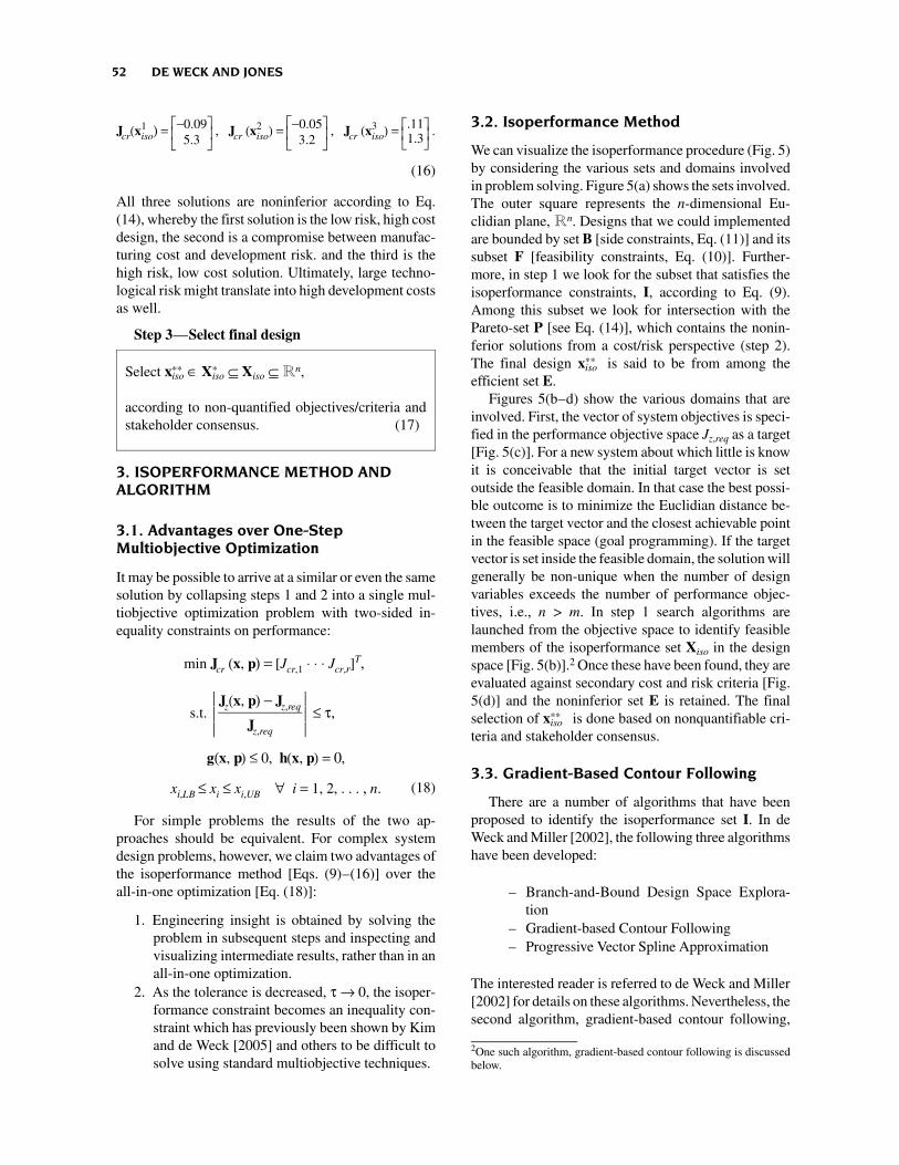
All three solutions are noninferior according to Eq.(14), whereby the first solution is the low risk, high costdesign, the second is a compromise between manufac-turing cost and development risk. and the third is thehigh risk, low cost solution. Ultimately, large techno-logical risk might translate into high development costsas well.

Step 3—Select final design

3. ISOPERFORMANCE METHOD ANDALGORITHM

3.1. Advantages over One-StepMultiobjective Optimization

It may be possible to arrive at a similar or even the samesolution by collapsing steps 1 and 2 into a single mul-tiobjective optimization problem with two-sided in-equality constraints on performance:

min Jcr (x, p) = [Jcr,1 ⋅ ⋅ ⋅ Jcr,r]T,

s.t.

Jz(x, p) − Jz,req

Jz,req

≤ τ,

g(x, p) ≤ 0, h(x, p) = 0,

xi,LB ≤ xi ≤ xi,UB W i = 1, 2, . . . , n. (18)

For simple problems the results of the two ap-proaches should be equivalent. For complex systemdesign problems, however, we claim two advantages ofthe isoperformance method [Eqs. (9)–(16)] over theall-in-one optimization [Eq. (18)]:

1. Engineering insight is obtained by solving theproblem in subsequent steps and inspecting andvisualizing intermediate results, rather than in anall-in-one optimization.

2. As the tolerance is decreased, τ → 0, the isoper-formance constraint becomes an inequality con-straint which has previously been shown by Kimand de Weck [2005] and others to be difficult tosolve using standard multiobjective techniques.

3.2. Isoperformance Method

We can visualize the isoperformance procedure (Fig. 5)by considering the various sets and domains involvedin problem solving. Figure 5(a) shows the sets involved.The outer square represents the n-dimensional Eu-clidian plane, Rn. Designs that we could implementedare bounded by set B [side constraints, Eq. (11)] and itssubset F [feasibility constraints, Eq. (10)]. Further-more, in step 1 we look for the subset that satisfies theisoperformance constraints, I, according to Eq. (9).Among this subset we look for intersection with thePareto-set P [see Eq. (14)], which contains the nonin-ferior solutions from a cost/risk perspective (step 2).The final design xiso

∗∗ is said to be from among theefficient set E.

Figures 5(b–d) show the various domains that areinvolved. First, the vector of system objectives is speci-fied in the performance objective space Jz,req as a target[Fig. 5(c)]. For a new system about which little is knowit is conceivable that the initial target vector is setoutside the feasible domain. In that case the best possi-ble outcome is to minimize the Euclidian distance be-tween the target vector and the closest achievable pointin the feasible space (goal programming). If the targetvector is set inside the feasible domain, the solution willgenerally be non-unique when the number of designvariables exceeds the number of performance objec-tives, i.e., n > m. In step 1 search algorithms arelaunched from the objective space to identify feasiblemembers of the isoperformance set Xiso in the designspace [Fig. 5(b)].2 Once these have been found, they areevaluated against secondary cost and risk criteria [Fig.5(d)] and the noninferior set E is retained. The finalselection of xiso

∗∗ is done based on nonquantifiable cri-teria and stakeholder consensus.

3.3. Gradient-Based Contour Following

There are a number of algorithms that have beenproposed to identify the isoperformance set I. In deWeck and Miller [2002], the following three algorithmshave been developed:

– Branch-and-Bound Design Space Explora-tion

– Gradient-based Contour Following– Progressive Vector Spline Approximation

The interested reader is referred to de Weck and Miller[2002] for details on these algorithms. Nevertheless, thesecond algorithm, gradient-based contour following,

Select xiso∗∗ ∈ Xiso

∗ ⊆ Xiso ⊆ Rn,

according to non-quantified objectives/criteria andstakeholder consensus. (17)

2One such algorithm, gradient-based contour following is discussedbelow.


will be briefly discussed here, since it illuminates aninteresting mathematical property of the isoperfor-mance approach.

Assume that we start searching for isoperformancesolutions from within the feasible domain F with astarting point xO. Furthermore, let

be the Taylor decomposition of the jth objective func-tion evaluated at xk, where

∇Jz,j =

∂Jz,j

∂x1

⋅ ⋅ ⋅ ∂Jz,j

∂xn

T (20)

is the gradient vector of the jth objective function withrespect to the design variable vector. Initially, we followthe steepest gradient vector to ensure that we move fromthe initial point xO to a point xk

iso that satisfies theisoperformance constraint. Once such a point has beenfound, the algorithm switches to “contour following”mode. Let xk = xk

iso be an isoperformance point that

satisfies Eqs. (9)–(11). To find additional isoperfor-mance points, the condition

∇Jz,jT x

k ∆x ≡ 0 (21)

must be satisfied. In other words, we want to findtangential directions that are performance invariant.Since this must be true for all performance objectives,j = 1, 2, . . . , m at once we define

to be the system Jacobian. This is the matrix of partialderivatives of the m performance objectives with re-spect to the n design variables. Performance invariantdirections can be found by singular decomposition ofthe Jacobian:

U Σ VT = ∇J zT (23)

Figure 5. (a) Venn diagram, (b–d) domains mapped in the isoperformance method.

(19)

(22)


The Σ matrix contains the singular values. Here we areinterested in the zero singular values. The correspond-ing columns of the V matrix span the nullspace of theJacobian.

Any linear combination of these n - m null vectorspoints in a performance invariant direction,

∆x = α ⋅ (β1vm+1 + . . . + βn−mvn) = αVoβ__

, (25)

where α is an arbitrary, but small, step size and β__

is avector of linear combination parameters. Hence, isop-erformance solutions can be obtained from the null-space of the system Jacobian matrix. Figure 6 shows fora sample problem (de Weck and Miller, [2002]) in threedimensions how the algorithm finds isoperformancesurfaces by following performance-invariant directionsin the nullspace.

In this paper we are particularly interested in con-tours and isoperformance surfaces that arise, when thevector Jz represents the performance of a complextechnical or human system. Thus, Jz could represent thepointing performance of a space telescope, average fueleconomy of a car, total output of an electrical powergrid, or the aptitude of humans as measured by someobjective criterion. In economics, relationships of thistype are usually called indifference curves. In sensorypsychology and physiology, they are often called iso-

frequency, isochronal or isoelectric curves or contours.These terms all share the prefix iso-, which means “thesame.” Graphically showing isoperformance results forn > 3 is challenging.

3.4. Physics-Based versus EmpiricalModels

From the discussion thus far it is clear that isoperfor-mance requires some mathematical model that relatesthe design vector x to both performance as well ascost/risk objectives, Jz and Jcr, respectively. The modelcan be derived from first principles [as was done in Eq.(1)], or obtained from empirical experimental or fieldobservation. In the first case the model is developed andimplemented directly (deterministic case). In the sec-ond case an empirical model (with embedded statisticaluncertainty) must be developed first. This requires adata set that relates experimental factors (x) to observedoutcomes (J). A variety of meta-modeling techniquessuch as response surfaces, kriging, or neural networksare available for this purpose, and there is an abundantliterature on this subject. Figure 7 illustrates these twocases. Note that the isoperformance algorithms used toextract the performance-invariant set Xiso, are the samein both cases.

The following two sections give examples of isoper-formance applications for both the deterministic case(spacecraft design) as well as the stochastic case (teamsports).

4. EXAMPLE 1: SPACECRAFT DESIGN

The design of precision optomechanical systems forremote sensing in space is challenging since it combinestightly coupled disciplines such as structures, optics andcontrols. When applied to space telescopes such as the“Nexus” spacecraft concept shown in Figure 8, we need

Figure 6. Gradient-based Contour-Following algorithm (n = 3, m = 1).

(24)


to ensure adequate optical performance, despite thepresence of various mechanical and electronic distur-bance sources. The system performance is captured bytwo criteria, Jz,1, which measures the root-mean-mean-square wave front error (RMMS WFE) and Jz,2, whichmeasures the root-sum-square (RSS) line-of-sight(LOS) image excursions on the focal plane. Both ofthese can be simulated using a computer model. Detailsof the model are presented in de Weck and Miller[2002]. The simulation results for Jz,2 are for an initialdesign xO and are shown in Figure 9.

The required pointing performance level, Jz,2,req = 5[µm], is driven by the size of a pixel on the focal plane(25 µm) so that images will not blur during long expo-sures. The time trace in Figure 9 represents the motionof the image centroid across the focal plane during 5 s

of simulated operations. If the motion is too large,collected photons will be spread over many pixels, andimage quality will deteriorate. Setting Jz,2,req to a tighterrequirement than 5 µm would not yield any benefit tothe system as a whole since the performance is inher-ently limited by pixel size. Enforcing a tighter require-ment or even demanding a “zero jitter” system wouldbe nonsensical and expensive. We see that initially

Figure 7. Deterministic versus empirical modeling approaches.

Figure 8. Simulation block diagram of Nexus spacecraftmodel.

Figure 9. Pointing performance simulation for Nexus spacetelescope system (T = 5 s simulation). Large black trace: initialdesign xO; small white trace: isoperformance design xA

iso.


system performance requirements are not met [Jz,2 (xO)= 14.97 µm]. An isoperformance analysis is performedon the system using the procedure described in Sections3.2 and 3.3.3

The performance of the system is a function of manydesign variables such as the ones shown in the Figure10. This plot is a graphical bar chart representation ofthe normalized Jacobian matrix of the system [Eq. (22)]evaluated at the initial design point xO. The 25 designvariables xi, i = 1, 2, …, n, are grouped into disturbancevariables and structural, optical, and controls subsystemvariables. It is the combination of these settings thatenables satisfactory system performance. While thedetails of the model are available elsewhere [de Weckand Miller, 2002], we can see that performance is mostsensitive to a subset of these variables (Table II). Iso-performance analysis was performed on this problem

and several hundred potential designs that would allmeet the performance requirement were identified.How to choose among these?

We introduce three secondary cost-risk objectivesthat are used to screen solutions from the isoperfor-mance set xiso:

— Jcr,1 = 1n

∑ i = 1

n

xi − (xi,LB + xi,UB) / 2

(xi,LB + xi,UB) / 2

= closeness to mid-range of design variables,

— Jcr,2 = Kcf

= magnitude of control gain,(26)

— Jcr,3 = ∑ i=1

n

∂Jz

∂xi

δxi

= sensitivity of performance to perturbations.3The other performance metric is simultaneously driven to a targetvalue of Jz,1,req = 20 µm.

Figure 10. Bar chart of normalized Jacobian matrix ∇Jz(xO) for space telescope design.


Minimizing the first of these objectives leads to adesign where, on average, most design variables will beclose to the midpoint between their upper and lowerbounds. Since extreme design variable values are oftendifficult or expensive to achieve, this metric achievesthe “best balance” between the various subsystemscontributing to overall performance (A). The secondmetric is geared towards minimizing the amount ofcontrol gain used. We might call this the “minimumenergy” design solution (B), while the third metriccaptures the isoperformance design that is least sensi-tive to uncertainties in the settings of individual designvariables (C). We might call this the “most robust”solution. Figure 11 shows a polar plot of these threeisoperformance designs (A, B, C), where the actualsettings of design variables xk

i,iso are shown in a normal-ized fashion.

Significant systems engineering insight can be de-rived from this representation. Design A allows almostall variables to be set close to a comfortable midrange,with the exception of Mgs (faint stars allowed) and Ru

(large wheel speed allowed), whose requirements canbe relaxed. Design B allows for a small control gain Kcf,but in order to still achieve performance, the distur-bances sources must be benign (e.g., small imbalances),the reaction wheel isolator must be soft (Kr,iso small)and the guide star signal strong (Mgs small value = large

brightness). Finally, Design C is the least uncertain, andwe can readily see that this is achieved by stronglysuppressing the design variables related to the distur-bance sources (Us, Ud, Ru) and building a stiff, massivestructural subsystem (Kr,iso, tsp are large). The perform-

Table II. Subset of the 10 Most Sensitive Design Variables (for Nexus Spacecraft)

Figure 11. Polar plot of three performance-invariant designs:A, B, and C.


ance levels for these three isoperformance designs aresummarized in Table III. Note that these designs arenoninferior with respect to each other, similar to thegeneric isopoints shown in Figure 5(d). A final decisionamong this small set of isoperformance designs cannotbe predicated on further analysis and optimization, butrequires stakeholder discussion and consensus. It is inthis sense that isoperformance enables engineering in-sight and acts as an enabling methodology for a target-driven systems engineering process.

5. EXAMPLE 2: TEAM PERFORMANCE INSPORTS

Systems involving human agents have been tradition-ally investigated in applied psychology and humanfactors engineering; see Jones et al. [Kennedy, Turnage,and Jones, 1996; Jones and Kennedy, 2000]. This leadsto a probabilistic variant of the isoperformance ap-proach, where contours of equal performance are ob-tained from empirical models [see Fig. 7(b)]. Modelscan take on the form of response surfaces such as

E[Jz,i] = a0 + a1(x1,i) + a2(x2,i)

+ a12(x1,i − x_

1)(x2,i − x_

2) + ⋅ ⋅ ⋅ , (27)

where E[ ] is the expectation operator, Jz,i is the per-formance of the ith individual, team or system, a0–a12

are fitting parameters, x1,i and x2,i are design variables4

and x_

1 and x_

2 are the mean values of a given data set.Jones and Kennedy [1996] have discussed the problemof finding the isoperformance curves of a baseball teamin terms of its final standings (FS = fraction of games

won at the end of the regular season) as a function ofthe team’s batting ability (x1 = RBI = runs batted in) andpitching ability (x2 = ERA = earned run average).5 Theyargue that RBI and ERA can be viewed as independentvariables, since the players responsible for achievingthese statistics are usually not the same. Teams with ahigh final standing (> 0.500) are expected to have bothgood pitching and batting, but for any realistic desiredfinal standing it would be desirable to obtain the trade-off curve between the two factors. The first step is tocompile the statistical data and to fit an empirical modelto it. The empirical model in the baseball examplebecomes

E[FSi] = a0 + a1(RBIi) + a2(ERAi)

+ a12(RBIi − RBI____

)(ERAi − ERA____

). (28)

The fitting parameters are obtained by compiling theERA, RBI, and FS standings from past seasons6 andoptimizing the fitting parameters using least-mean-squares. For the baseball team model [Eq. (28)] weobtain a0 = 0.7450, a1 = 0.0321, a2 = –0.0869, and a12

= –0.0369. The standard deviation error of the empiricalfit is σε = 0.0493. The second step is to determine theexpected level of performance for team i such that theprobability of adequate performance is equal to thespecified confidence level. We write

E[Ji] = Jreq + zσε, (29)

where E[Ji] is the expected level of performance of teami, Jreq is the desired (required) final standing at the end

Table III. Comparison of Performance, Cost, and Risk Objective Values for Three Performance- Invariant Designs: A, B, and Ca

4“Determinants” as they are referred to in the Human Factor litera-ture.

5The third major category are the fielding statistics, which are ignoredhere.6The 2000 and 2001 major league baseball (MLB) results are usedhere (60 data points = 2 seasons × 30 teams).

a Isoperformance tolerance τ = 0.05.


of the season, z is the confidence level obtained from anormal distribution lookup table of the Gaussian distri-bution function

Φ(z) = 1

√2π ∫ −∞

z

e− z

2

2 dz, (30)

and σε is the aforementioned model fitting error. Thisassumes that the error for the empirical model followsa normal distribution. Let the decision-maker (e.g.,team owner “i”) decide that the required final standingfor his team should be FSi = 0.550 and that the prob-ability that this result (performance) should be achievedis 80%. We obtain the expected final standing (targetperformance) as

E[FSi] = .550 + zσε = .550 + 0.84(0.0493) = 0.5914. (31)

In other words, if the final standing FS of team i is toequal or exceed 0.550 with a probability of 80%, thenthe expected final standing for team i must equal0.5914. Finally, the isoperformance contour for thisperformance level (Fig. 12) can be obtained analyticallyor with one of the algorithms discussed in Section 3.3as

RBIi = .5914 − a0 − a1ERAi + a12RBI

____ (ERA i − ERA

____)

a1 + a12(ERAi − ERA____

).

(32)

Some interesting conclusions can be drawn from thiscurve (Fig. 12). The performance measure FS seems to

be more sensitive to changes in pitching performance(ERA) than in batting performance (RBI), which sup-ports the commonly held opinion that pitching is moreimportant than batting in major league baseball. Also,as the team goal (FS) becomes more ambitious, thenumber of options or length of the isoperformancecontour becomes smaller. Most to the point, the desiredfinal standing can be achieved with an excellent pitch-ing staff (ERA = 3.0) and modest batting (RBI = 4.2)or conversely with a stellar team at bat and a lesserpitching staff (RBI = 6.0 and ERA = 4.2). It is interest-ing to note that the best team (Atlanta Braves) and worstteam (Chicago Cubs) have nearly identical RBI, butsignificantly different ERA. The FS for the Braves issomewhat underpredicted by the empirical model dueto its inherent stochastic nature. The role of ERA in thissituation is reminiscent of the role of Isp in the rocketdesign example of Section 1.

Once an isoperformance curve has been selected,say, 0.5914, as the goal to be achieved, the next step isto decide which points along this curve to pursue. Thisdecision will almost always depend on where the teamcurrently stands with respect to ERA and RBI. If a teamalready has outstanding pitching but not-so-outstandingbatting, it may be easier to find batters who will nudgethe team toward its goal than pitchers. It may also beless expensive, since even better pitchers than the teamalready has are likely to be very expensive. Detailedanalyses may reveal many particular ways that a teamcould produce a better ERA or RBI. Each of thesepossibilities can be examined with respect to feasibility,cost, and how closely it promises to put the team on theselected isoperformance curve. In the end, of course,management must decide which course to follow, butthe isoperformance analysis will have guided the deci-sion-making process from its beginning.

6. SUMMARY AND CONCLUSIONS

Isoperformance is as much a system design philosophyas an operational method. It is true that traditionalengineering education and practice heavily emphasizesystem performance optimization. In reality, however,the notion of optimality for large, complex systems issomewhat less clear. This paper argues that traditionaloptimization of system performance is not the onlyreasonable approach in the design and analysis of com-plex systems. Isoperformance, a complementary ap-proach, does not seek the extremes of systemperformance, but enforces that the system meet prede-termined performance targets (= requirements). Thisensures that the system is neither grossly over- norunderdesigned. What can be gained by this approach?

Figure 12. Major league baseball isoperformance analysis(2000–2001 data).


Three potential benefits arise from use of the isoperfor-mance method:

1. It considers not just a single, “optimal” pointdesign but a family of performance-invariant,noninferior designs in terms of other cost and riskcriteria.

2. Designs can be found, within the performanceinvariant set, such that the burden for achievingthe system performance is well “balanced”among subsystems.

3. It offers greater insights into the inherent trade-offs between performance, risk, and cost andallows system analysts and designer to be moreinteractive, compared to “push-button” optimiza-tion.

One may consider performance as a surrogate “cur-rency” for complex systems that are composed of tech-nical and human elements. The fact that suboptimalsystem performance is acceptable in many cases allowsconsidering the margin between “optimal” perform-ance and the lesser, required performance along theisoperformance contours as a resource. This perform-ance margin can be viewed as a “currency” that can beinvested in different ways: making the system moreaffordable to implement, more robust or flexible, suchas enabling upgrades after initial fielding has occurred.

One may argue that similar results could be obtainedby an all-in-one multiobjective optimization [Eq. (18)].The question regarding which of the two approaches,multiobjective optimization or isoperformance, is supe-rior for the design of complex Engineering Systems isnot easy to answer or necessarily relevant as they canbe viewed as complementary. It is, however, wellknown that most optimization algorithms experiencesignificant difficulties and computational expensewhile enforcing equality constraints, and this is themain strength of isoperformance.

The isoperformance approach decouples the prob-lem into three phases that allow system analysts anddesigners to develop intuition about system tradeoffsthat would otherwise remain hidden. The approach doesnot rely on stakeholder preferences except for the selec-tion of the final design, xiso**, from the efficient set E.

Future work includes extending isoperformance todesign problems where both discrete and continuousdesign variables are present. This is important, as manyarchitectural variables (number of stages in rocket de-sign, Cassegrain versus Gregorian telescope concept,etc.) are discrete in nature and can have a great impacton system performance, cost and risk. Also, of the fourtensions shown in Figure 2 we have not explicitly dealtwith schedule. To do so would require combining isop-

erformance analysis and multidisciplinary design opti-mization with a quantitative model of project manage-ment. One could envision a framework where changesin system performance targets are propagated tochanges in the associated design variables, which inturn cause schedule impact on the associated designtasks. Work on integrating system design with projectmanagement is difficult, but essential for those organi-zations that strive for excellence and balance acrosscompeting demands in complex system design.

NOMENCLATURE

τ Isoperformance tolerance level (fraction of nominal performance)

d Exogenous system disturbance inputm Number of system performance objec-

tivesn Number of design variablesp System fixed parameterr Reference input signal, Number of

cost-risk objectivesu System control inputw Filtered disturbance inputxi ∈ R Continuous design variabley System outputz System performance (filtered system

output)Gsys, GI, GO System transfer function matricesJi, Jreq,i System objective, required perform-

ance levelK Controllerp Vector of fixed parametersx Design variable vectorJ System objective vector

REFERENCES

H.E. Cook, Product management: Value, quality, cost, price,profits and organization, Chapman & Hall, New York,1997.

O.L. de Weck and D.W. Miller, Multivariable isoperformancemethodology for precision opto-mechanical system,AIAA-2002-1420, 43rd AIAA/ASME /ASCE/AHSStruct Struct Dyn Mater Conf, Denver, Colorado, April22–25, 2002.

J.J. Gilheany, Optimum selection of dampers for freely vibrat-ing multi-degree of freedom systems, Proc Damping ’89,II, 1989, pp. 1–18.

M.B. Jones, Isoperformance and personnel decisions, HumFactors 42(2) (2000), 299–317.

M.B. Jones and R.S. Kennedy, Isoperformance curves inapplied psychology, Hum Factors 38(1) (1996), 167–182.


R.S. Kennedy, J. Turnage,. and M.B. Jones, A meta-model forsystems development through life cycle phases—cou-pling the isoperformance methodology with utility analy-sis, SAE PAPER 901947, SAE Aerospace TechnologyConference and Exposition, Long Beach, CA, 1990.

H.J. Kim, C. Kim, and O.H. Rho, Multipoint inverse designmethod for transonic wings, J Aircraft 36(6) (1999), 941–947.

I.Y. Kim and O.L. de Weck, Adaptive weighted-sum methodfor bi-objective optimization: Pareto front generation,Struct Multidisciplinary Optim 29(2) (2005), 149–158.

M.W. Maier and E. Rechtin, The art of systems architecting,2nd edition, CRC Press, Boca Raton, FL, 2000.

A. Messac, Physical programming: Effective optimization forcomputational design, AIAA J 34(1) (1996), 149–158.

S.J. Osher and R.P. Fedkiw, Level set methods and dynamicimplicit surfaces, Springer, New York, 2002.

V. Pareto, Manuale di economia politica, Societa EditriceLibraria, Milano, Italy, 1906. Translated into English byA.S. Schwier as Manual of political economy, Macmillan,New York, 1971.

D. Schrage, et al. Current state of the art on multidisciplinarydesign optimization, An AIAA White Paper, URL refer-ence: http://endo.sandia.gov/AIAA_MDOTC/spon-sored/aiaa_paper.html, AIAA Multidisciplinary DesignOptimization, Technical Committee, September 1991.

R. Shishko, R.G. Chamberlain, et al., NASA systems engi-neering handbook, SP-610S, NASA, Washington, DC,June 1995.

H.A. Simon, The sciences of the artificial, 3rd edition, MITPress, Cambridge, MA, 1996.

K. Tsiolkovsky, The exploration of cosmic space by means ofreaction motors, Scientific Review, Moscow and St. Pe-tersburg, 1903.

Olivier L. de Weck is currently an assistant professor with a dual appointment between the Departmentof Aeronautics and Astronautics and the Engineering Systems Division (ESD) at MIT. His researchinterests are in Integrated Modeling and Simulation, Multidisciplinary Design Optimization, and SystemArchitecture. In 2001 he obtained a Ph.D. in Aerospace Systems from MIT. From 1987 to 1993 he attendedthe Swiss Federal Institute of Technology (ETH Zurich) in Switzerland, where he earned a DiplomIngenieur degree (MS equivalent) in industrial engineering. From 1993 to 1997 he served as liaisonengineer and later as engineering program manager for the Swiss F/A-18 program at McDonnell Douglas(now Boeing) in St. Louis, MO. He is serving as the General Chair for the 2nd AIAA MultidisciplinaryDesign Optimization (MDO) Specialist Conference in 2006 and obtained two best paper awards at the2004 INCOSE Systems Engineering Conference.

Marshall B. Jones is professor emeritus of Behavioral Science at The Pennsylvania State University andwas for 24 years chairman of that department in the College of Medicine. He has conducted extensiveresearch in human factors, psychiatric genetics, especially the genetics of autism, the spread of attitudesand behaviors from one person to another, and the prevention of antisocial behavior. He currently servesas board chairman of Keystone Human Services, a large behavioral health organization headquartered inCentral Pennsylvania but active in Connecticut, Maryland, Delaware, and, recently in Eastern Europe, aswell as in Pennsylvania. Jones received his B.A. degree from Yale in 1949 and his Ph.D. from the Universityof California at Los Angeles in 1953.


Regular Paper Isoperformance: Analysis and Design of ...

Documents

Transcript of Regular Paper Isoperformance: Analysis and Design of ...