Regressor Dimension Reduction with Economic

Constraints: The Example of Demand Systems with

Many Goods

Stefan Hoderlein and Arthur Lewbel

Boston College and Boston College�

original Nov. 2006, revised Feb. 2011

Abstract

Microeconomic theory often yields models with multiple nonlinear equations, nonsep-

arable unobservables, nonlinear cross equation restrictions, and many potentially mul-

ticollinear covariates. We show how statistical dimension reduction techniques can be

applied in models with these features. In particular, we consider estimation of derivatives

of average structural functions in large consumer demand systems, which depend nonlin-

early on the prices of many goods. Utility maximization imposes nonlinear cross equation

constraints including Slutsky symmetry, and preference heterogeneity yields demand func-

tions that are nonseparable in unobservables. The standard method of achieving dimen-

sion reduction in demand systems is to impose strong, empirically questionable economic

restrictions like separability. In contrast, the validity of statistical methods of dimension

reduction like principal components have not hitherto been studied in contexts like these.

We derive the restrictions implied by utility maximization on dimension reduced demand

systems, and characterize the implications for identi�cation and estimation of structural

marginal e¤ects. We illustrate the results by reporting estimates of the e¤ects of gaso-

line prices on the demands for many goods, without imposing any economic separability

assumptions.

JEL codes: D12, C30, C43, C14. Keywords: Demand System, Dimension Reduction, Mar-

shallian demands, Separability, Testing Rationality, Nonparametric, Gasoline prices.�Stefan Hoderlein, Department of Economics, Boston College, 140 Commonwealth Ave., Chestnut Hill, MA,

02467, USA, email: stefan_hoderlein@yahoo.com. Arthur Lewbel, Department of Economics, Boston Col-

lege, 140 Commonwealth Ave., Chestnut Hill, MA, 02467, USA; lewbel@bc.edu, http://www2.bc.edu/~lewbel/

Excellent research assistance by Sonya Mihaleva is gratefully acknowledged.

1

1 Introduction

Consider a policy question like, "what would be the e¤ects of an increase in gasoline taxes

or prices on the demands for every good consumers purchase?" By standard utility theory,

Marshallian demand functions for each good depend (typically nonlinearly) on the prices of

every consumption good. The number of di¤erent goods that consumers buy is large, and

observed price variation across consumers in most data sets is limited (since, absent price

discrimination, all consumers in a given time period and region pay similar if not identical

prices). As a result, available data sets do not have su¢ cient price variation to estimate demand

functions containing the separate prices of all the dozens or hundreds of di¤erent goods that

theory says must be considered.

This is a common problem in many microeconometric applications. Structural models of-

ten involve large numbers of covariates, yielding the curse of dimensionality in nonparametric

models. Even in semiparametric and parametric models, having large numbers of closely re-

lated regressors, like many prices, often leads to multicolinearity, �at objective and likelihood

functions, and related problems. The di¢ culties associated with having many regressors are

exacerbated in contexts like demand systems both by the constraints of utility theory and by

the complexity of empirically observed behavior, which together require models that are highly

nonlinear, have complicated nonlinear cross equation restrictions, and possess nonseparable

vectors of unobserved preference heterogeneity parameters. To deal with these problems, we

show how statistical dimension reduction techniques like principal components can be applied

in this context of nonlinear, nonseparable, multiple equation systems.

The typical way of dealing with these di¢ culties is to impose strict constraints on behavior

using, e.g., strong restrictions on preferences such as separability. In the demand system con-

text, both traditional separability assumptions (Gorman 1959, Blackorby, Primont, and Russell

1978) or modern variants like latent separability (Blundell and Robin 2000) greatly restrict pref-

erences by assuming that very many ad hoc equality constraints exist on the cross price e¤ects

of goods within each group.1 The limitations of these grouping schemes become obvious when

the goals of the analysis concern prices and demands of individual goods, since separability into

groups forces common price e¤ects on all goods within each group. Alternatives to separability

such as the Hicks (1936) and Leontief (1936) composite commodity theorem or the newer gen-

eralized composite commodity theorems (Lewbel 1996, Davis 2003) permit estimation of group

demands without separability, but cannot provide estimates of the e¤ects of prices and income

1The undesirable result is that, to empirically implement modern �exible models that reduce or eliminate

restrictions on second and higher order cross price elasticities between groups, empirical practioners have as-

sumed a greater degree of separability (fewer groups), thereby implicitly imposing severe restrictions on the �rst

order cross price elasticities of individual goods within groups

2

on the demands for individual goods.

Analogous to separability assumptions are restrictions commonly imposed in the marketing

and industrial organization literatures in which demand functions are taken over a small number

of characteristics rather than over a large number of goods (as in hedonic pricing models) and

typically restrict goods to discrete choices. A prominent example is Berry, Levinsohn, and

Pakes (1995). These methods work well when the number of characteristics describing goods

is small relative to the number of goods (as when the goods consist of many brands of a single

type of product) and when quantities purchased tend to be small and hence well approximated

by discrete counts, like automobile purchases. In contrast, our proposed method can be applied

when the relevant set of characteristics is large or di¢ cult to enumerate, as when the goods are

diverse such as food, clothing, gasoline, etc.,. and when purchases are better approximated by

continuous quantities rather than discrete counts, as in gallons of gasoline per year.

As an alternative to these strong (and in many contexts, empirically questionable) economic

restrictions, we propose the use of statistical methods of dimension reduction like principal com-

ponents to identify the marginal e¤ects (derivatives or elasticities) of continuous covariates of

interest on average structural functions in nonlinear, nonseparable models possessing economic

constraints. The validity of statistical methods of dimension reduction has not hitherto been

studied in contexts like ours of nonseparable errors and nonlinear cross equation restrictions.

For concreteness, we illustrate our approach using demand systems. The speci�c complica-

tion for demand systems is that they possess as many prices as there are equations (goods), the

prices of all goods appear (generally nonlinearly) in all equations, unobserved random utility

parameters appear nonadditively and nonseparably in every equation, and utility maximiza-

tion yields nonlinear functional restrictions such as homogeneity and Slutsky symmetry both

within and across equations. However, given the preceding discussion it should be clear that

our basic methodology can be generalized to other high dimensional economic models with

many continuously distributed covariates.

To describe our main contribution, consider the following set up: Let P1 be a small vector

of regressors of interest to the researcher, in our case the log price of gasoline, and let P2 be

the much larger vector of other regressors, in our case logged prices of all the other goods that

consumers buy. In ordinary linear regression models, a standard solution to multicollinearity

is to replace the large set of multicollinear nuisance regressors, in this case P2, with a much

smaller set of regressors R2 constructed by applying a principal components, factor analysis, or

other statistical dimension reducing algorithm to P2 (see, e.g., Judge et. al. 1985 chapter 22).

We consider a similar solution to multicollinearity in the context of the nonlinear, nonseparable

set of equations that comprise consumer demand systems with random utility parameters.

Note that the issue we are addressing is not lack of price variation per se, but multicollinear-

3

ity. If almost all of the variation in prices P2 is driven by a small number of factors, then the

elements of P2 will be highly multicollinear, corresponding to insu¢ cient relative price varia-

tion among all the prices. In contrast, the principal components will consist largely of these

few factors, which can possess su¢ cient variation relative to each other over time to strongly

identify their separate e¤ects on demand.

Our �rst result establishes conditions under which the derivatives of dimension reduced

nonparametric regressions involving P1 and R2 (in place of P1 and P2) can be used to obtain

derivatives of average structural functions in the sense of Blundell and Powell (2004), Altonji

and Matzkin (2005), or Hoderlein (2005) and Hoderlein and Mammen (2007). Under suitable

assumptions we show a direct link between average structural derivatives and the derivatives of

constrained low dimensional regressions, but in the most general case obtaining these derivatives

requires an empirically estimable additional correction term.

A second set of results takes this �rst result as a building block and considers implica-

tions and restrictions arising from economic theory in the dimension reduced regression. We

assume that individuals purchase quantities of many di¤erent goods to maximize utility func-

tions (that may vary in unobserved ways across individuals) under a linear budget constraint,

yielding Marshallian demand equations that are functions of P1 and P2 which possess certain

testable restrictions (the so called integrability constraints). We derive the restrictions on the

dimension reduced nonparametric demand functions involving P1 and R2 that arise from ap-

plying dimension reduction to the original integrability constrained Marshallian demands that

are functions of P1 and P2.

For example, we show that the dimension reduced demand functions do not themselves

satisfy Slutsky symmetry (their Slutsky matrix is not even square) but under general conditions

a certain transformation of them is symmetric. We emphasize that no form of separability or

two stage budgeting is assumed in this analysis. Dimension reduction based on replacing P2 with

R2 is accomplished solely by exploiting mostly testable restrictions on relative price movements

rather than di¢ cult to test separability restrictions on preferences.

In our empirical applications, we apply these results to estimate the underlying structural

derivatives of dependent variables (in our application, a large collection of budget shares) with

respect to a regressor of interest (log gasoline price), and we estimate similar semi-elasticities

with respect to other regressors such as total expenditures and demographic characteristics.

Our theorems employ elements of Brown and Walker (1989), Lewbel (2001), Christensen

(2004), and Hoderlein (2005) regarding unobserved preference heterogeneity, and Lewbel (1996)

and Davis (2003) regarding price dimension reduction. However, by combining and extending

these methods, we obtain far more general results. In particular these earlier paper can only

identify aggregate e¤ects across aggregates of goods, while we, e.g., identify the average e¤ect

4

of the price of gasoline on each of the many di¤erent goods that individuals buy, not just group

price e¤ects.

While our modeling method and associated identi�cation results are new, the resulting

estimators take a standard two step estimation form, involving parametric or nonparametric

regressions (the demand system) which are estimated with some ordinary regressors such as P1and some generated regressors, R2, so no new or nonstandard limiting distribution theory is

required.

To show how our dimension reducing technique applies in di¤erent settings, we provide

two empirical applications. The �rst is a simple parametric aggregate consumer model that

illustrates the basic methodology and provides some macroeconomic estimates of gasoline own

and cross price e¤ects. The second application is a fully nonparametric individual consumer

level study, which permits direct estimation and rigorous testing of the modelling methodology

without household aggregation or functional form restrictions. Both applications show that our

approach is easily implemented, obtains economically plausible results and provides a convenient

was of dealing with the problem of the dimensionality of the vector of regressors in large

structural econometric models.

2 The Model

In this section we introduce the model formally, lay out the basic assumptions, and provide an

in depth discussion of the economic content of the model in the case of consumer demand.

2.1 Notation

Let P1 be a J1 vector of regressors of interest, in our application logged prices, and let P2 be a

large J2 vector of other regressors, in our case the logged prices of all other goods. Let P be the

J = J1+J2 vector of the logged prices of all goods, so P 0 = (P 01 : P02) where

0 denotes transpose.

Let R be the K vector (with K much smaller than J) de�ned by R0 = (P 01 : R02), so R consists

of the logged prices of interest, P1, and some summary measures, R2, of the remaining logged

prices P2. Let W be the J vector of budget shares of all goods consumed, so each element of

W is the fraction of total expenditures spent on a good, and the corresponding element of P

is the price of that good. The elements of W are nonnegative and sum to one. De�ne Y to

be logged total expenditures, and let Z denote a vector of other observable characteristics of

consumers that a¤ect, determine, or covary with their preferences. The vector Z might include

variables like household size, age, sex, region, and home ownership status. Finally, let A be a

vector of all unobserved characteristics that a¤ect preferences and hence demand.

5

The notation using capital letters re�ects the fact that these variables are random, varying

across the population and time. Realizations of these variables are denoted by small letters,

when necessary with subscripts as yit, wit, zit, ait, and pt, where i indexes the consumer and t

indexes the price regime, where prices may vary by location as well as by time. Let jj � jj denoteEuclidean norm, let vec denote the vectorization operator. Let FAU denote the joint cdf of two

random vectors A and U , and fAU denote the joint pdf. Finally, let E denote expectation.

2.2 Assumptions

Using this notation, we are now able to state our assumptions formally. The �rst speci�es the

outcome equation of interest:

Assumption 1 Let (;F ;P) be a complete probability space on which are de�ned therandom vectors A : ! A; A � R1; and (W;P; Y; Z) : !W �P � Y � Z; W � RJ ;P �RJ ;Y � R;Z � RL; t = 1; 2; with J and L �nite integers, such that (i)

W = �(P; Y; Z;A);

where � : P � Y � Z �A !W is a Borel measurable function; and (ii) realizations of

W;P; Y; Z are observable, whereas those of A are not.

Although this and later assumptions may apply to many general contexts, we will for con-

creteness discuss and interpret them in a consumer demand scenario: The function � describes

our large scale structural model in a heterogeneous population, involving all regressors as well

as observed and unobserved heterogeneity parameters Z and A. If � comes from utility max-

imization, then we may think of A as random utility parameters where the variation is either

across individuals or across unobserved factors that determine preferences, while Z are ob-

servable characteristics that a¤ect utility, so each consumer�s utility function is completely

determined by Z and A. When holding Z and A �xed, � as a function of P and Y is the vector

of Marshallian budget share demand functions. At this level of generality, each consumer can

have a utility function, and associated Marshallian demands, that are completely di¤erent from

everyone else�s. Since A � R1, the vector A can have any dimension.We assume that demand functions involving all prices cannot be estimated with any useful

precision because the J vector P is too large and multicollinear, so we instead consider demand

equations W = m(R; Y; Z) + V , where m is de�ned as the conditional expectation of W

conditioning on R, Y , and Z. The error vector V embodies the e¤ects both of variation in

unobserved taste attributes A across consumers and the e¤ects of variation in P2 that are not

captured by variation in R.

6

In order to link the large set of regressors P to the dimension reduced set R, we introduce

the following assumption:

Assumption 2 (i) There exists a J vector U and a J by K matrix of constants � such

that

P = �R + U (1)

where � has rank K and all rows of � sum to one.

(ii) Moreover, � is continuously di¤erentiable in the �rst J +1 components and there exists

a function � such that

jj�Dy�(�r + u; y; z; a)

0 : vec [Dr�(�r + u; y; z; a)]0� jj � �(u; a);

withR�(u; a)FAU(da; du) <1; uniformly in (r; y; z):

By itself, Assumption 2(i) can be interpreted as simply de�ning a vector U given a suitable

matrix �. The restriction that rows of � sum to one is a convenient scale normalization on the

elements of R and rules out trivial cases like � = 0. The �rst J1 elements of P and R are the

same vector P1, so the top left J1 by J1 corner of � is the identity matrix, the top right J1 by

K�J1 corner of � consists of zeroes, and the �rst J1 elements of U are identically zero. De�neU2 to be the J2 vector of remaining, nonzero elements of U . Note that since t indexes price

regimes, realizations of R;U may be denoted rt; ut.

Assumption 2(i) generally holds if the elements of R are de�ned as linear homogeneous

functions of P , that is, if R = �P for some matrix �, because if there exists a nonsingular

matrix S having �rst K rows equal to �, then write S�1 as (� : T ) and equation (1) holds with

U de�ned as T times the bottom J � K rows of S times P . An example is de�ning R as K

suitably scaled principal components of P , which is a standard method of obtaining dimension

reduction in linear regression models. Having R = �P is also a common way to construct

price indices R, e.g., a Stone index has this form with rows of � corresponding to budget share

weights. We will therefore refer to R, and in particular R2, as log price indices.

We will later assume that R and U are uncorrelated or independent. There are many di¤er-

ent models of price behavior that give rise to Assumption 2 with these additional restrictions.

For example, equation (1) with R independent of U is the structure of a standard factor analysis

model for log prices, and could also arise as a cointegration model for nonstationary log prices,

with R being I(1) processes, U equaling independent stationary processes, and K being the

number of cointegrating relationships that hold amongst the J logged prices.

A special case of Assumption 2(i) is the generalized composite commodity decomposition

of prices proposed in Lewbel (1996). In that model, R is a vector of price indices for distinct

groups of goods, each row of the matrix � has one element equal to one and all other elements

7

equal to zero, and U is a vector of di¤erences between group prices and the prices of individual

goods. Even when prices satisfy this particular decomposition, we still obtain results that di¤er

from, and are more general than, those of Lewbel (1996).

Assumption 2(ii) assumes di¤erentiability of the structural demand functions, and provides

a mild boundedness condition on the derivatives required to interchange di¤erentiation and

integration.

We now provide our main identify assumptions regarding the joint distribution of the ob-

servables and unobservables in our model.

Assumption 3: The joint distribution of R, Y , Z, A, and U obeys the following restric-

tions:

(i) (R;U) is independent of (Y; Z;A) :

(ii) A is conditionally independent of Y , conditioning on Z.

(iii) (A;U) are jointly absolutely continuously distributed with respect to Lebesgue measure,

conditional on (Y; Z;R).

Assumption 3(i) says that prices are determined independently of the variables that deter-

mine a consumer�s demand functions. This price independence implies that we are performing a

partial equilibrium analysis. Strictly, this assumption can only hold when prices are determined

exclusively by supply (e.g., if goods are produced by constant returns to scale technologies and

provided by perfectly competitive suppliers). However, for individual consumer data it is a

reasonable assumption under much more general conditions because the contribution of any

one consumer�s demands to aggregate demand, and hence to price determination, is in�nitesi-

mal. However, this does rule out possible e¤ects of common demand shocks. This assumption

also limits the possibility of including leisure as a good in the model, because it would then

restrict permitted relationships between an individual�s price of leisure (his wage rate) and

other variables that a¤ect demand.

In the Appendix we show that it is possible to relax assumption 3(i) if necessary, at the

expense of adding additional terms to the analysis that, while identi�ed in theory, may be

di¢ cult to estimate in practice. In one of our empirical applications, which uses aggregate

data, we consider instrumenting prices with supply side variables, which serves as a check on

the sensitivity of our results to possible violations of this assumption.

Assumption 3(ii) says that total expenditures are conditionally independent of random util-

ity parameters. This assumption a¤ects the variables that must be included in the conditioning

set Z. For example, if a consumer�s age a¤ects his or her preferences, and if age is correlated

with total expenditures, then age must be included in the vector of observed characteristics Z

to satisfy this assumption. This assumption is implicit in most empirical demand system appli-

8

cations, either because such models assume no unobserved variation in preferences, or because

all unobserved variation is assumed to be contained in ordinary model errors.

Assumption 3(iii) states that the unobservables are continuously distributed, which is stronger

than necessary but simpli�es some derivations. Taken together, the components of Assumption

3 immediately imply that fAU jY ZR = fU jRfAjZ .

Assumptions 1-3 comprise the core set of assumptions about our structural model, and we

derive general version of our results under these assumptions in the Appendices. To obtain

simpler (but more empirically convenient) results we invoke additionally the following assump-

tion.

Assumption 4: R and U are independently distributed.

Though Assumption 4 is clearly restrictive, it holds for example given a standard factor

analysis model for prices. Also, Lewbel (1996) and Davis (2003) provide empirical support

for this assumption for the special case of the generalized composite commodity model. This

assumption may be more problematic for prices of goods of interest that are included in R,

such as gasoline prices in our empirical application. This potential problem can be addressed

in two ways. First, Assumption 4 can be easily tested empirically, e.g., one possible test could

be based on regressing the estimated U residuals squared on a second degree polynomial in

R, analogous to White�s test for heteroskedasticity. Second, in an appendix we provide more

general results that do not depend Assumption 4. These extensions can be used in applications

where R is constructed to be uncorrelated with U , but not necessarily independent, e.g., when

U is de�ned as the residual from regressing P on R. For Assumption 4 it is not necessary to

assume that U has mean zero.

It is useful to compare these assumptions to those that are required for the standard methods

of obtaining dimension reduction in demand systems, which are behavioral separability restric-

tions. First, starting again from Assumption 1, standard demand system estimation does not

allow for unobserved heterogeneity A, or at most permits restrictive separable forms that ap-

pear only in additive error terms. See Lewbel (2001) for a fuller discusion of this point. Next,

for dimension reduction even weak separability requires that the cross derivatives of utility with

respect to any two goods in di¤erent groups be proportional to the cross derivatives of any other

pair of goods in those two groups (see, e.g., Blackorby, Primont, and Russell (1978) for details

on this and alternative stronger forms of separability). For estimation, one would also require

that every consumer in the sample have the same grouping of goods, and that the econometri-

cian knows a priori which goods go into which groups. It is also required that the subutility

functions for each group be known to the econometrician, so that price indices for each group

can be constructed prior to estimation of the across group demand functions. Virtually all of

9

these very strong behavioral assumptions required for traditional demand system estimation

are di¢ cult to test empirically, because doing so requires estimation of the non-dimension re-

duced demand system, and the whole reason for dimension reduction is precisely the inability

to estimate a non-dimension reduced system with any precision. So, for empirical work, the

restrictiveness of Assumptions 2, 3 and 4 should be assessed relative to these alternatives.

2.3 Objects of Interest

The goal of our analysis is to relate properties of the unobservable vector of demand func-

tions W = �(P; Y; Z;A) to the observable, empirically tractable dimension reduced regression

m(R; Y; Z), de�ned as

m(r; y; z) = E [W j R = r; Y = y; Z = z] = E [�(P; Y; Z;A) j R = r; Y = y; Z = z] :

This conditional expectation always exists because budget shares W are bounded. We call

�(p; y; z; a) the theoretical demand function andm(r; y; z) the empirical demand function, since

the latter is what we may feasibly estimate.

The empirical demand function m(r; y; z) above can be compared to the demand functions

m� that are usually estimated in practice, W = m�(P; Y; Z) + V � where V � is a vector of

model errors. Traditionally, one would make su¢ cient separability assumptions to reduce P

and W to manageable dimensions, and would assume that m�(p; y; z) itself equals the demand

functions arising from utility maximization, so rationality properties like homogeneity and

Slutsky symmetry would be imposed on (or tested with) m�. This would be a valid assumption

if, e.g., all consumers with the same value of z had identical preferences and if V � corresponded

to classical measurement errors. In that case, all of the Theorems in this paper would hold

replacing � with m�. However if V � is instead the residual obtained from de�ning m� as the

conditional expectation of � given p; y; z, then V � would be the e¤ect of variation in unobserved

preference attributes A, and m�(p; y; z) need not satisfy rationality properties. See, e.g., Brown

and Walker (1989), Lewbel (2001), Christensen (2004), and Hoderlein (2005), who derive and

test properties of m� and V � in this context.

In the present paper we do not deal with m�, since empirically feasible estimation of m�

requires additional restrictions such as separability. We instead directly condition the underly-

ing theoretical demand functions � on Y; Z, and a set of dimension reducing price indices R to

obtain the empirical demand function m(r; y; z) that can be estimated.

It is important to recognize that there is no one �correct�de�nition of R, and the resulting

demand functions we estimate depend on the choice of R. The underlying behavioral model

�(p; y; z; a) does not depend on R. As we show in the next section, the demand functions and

associated elasticities we estimate are essentially averages across goods and prices. So, e.g.,

10

if one is primarily interested in own and cross price elasticities for food, one would construct

R di¤erently than if the focus is on energy, analogous to the way one can estimate di¤erent

averages by grouping data in di¤erent ways, though the underlying data generating process

does not depend on how the data are grouped.

3 Marginal E¤ects of Interest

We�rst consider how the marginal e¤ects of interest, the income and price derivatives,Dym(r; y; z)

andDrm(r; y; z) of the dimension reduced regression relate to the theoretical onesDy�(p; y; z; a)

and Dp�(p; y; z; a). Note that these derivatives are semielasticities, that is, they are derivatives

of budget shares with respect to log total expenditures y and with respect to log prices p or log

price indices r. More rigorous statements of the assumptions and theorems along with some

generalizations and associated proofs are provided in the Appendix.

Theorem 1: Let Assumptions 1,2, and 3 hold. Then

Dym(r; y; z) = E [Dy�(P; Y; Z;A) j R = r; Y = y; Z = z] : (2)

If Assumption 4 also holds then

Dr1m(r; y; z) = E [Dp1�(P; Y; Z;A) j R = r; Y = y; Z = z] (3)

and

Drm(r; y; z) = E [Dp�(P; Y; Z;A) j R = r; Y = y; Z = z] � (4)

The Appendices contain the proofs of this and more general versions of this theorem where

we dispense in particular with the restrictive Assumption 4. Equation (2) shows that the

income semielasticities of the empirical demands are a best approximation (in the sense of

closest projection) to the theoretical income semielasticities, since they equal the conditional

expectations of the theoretical elasticities conditioning on the usable data R; Y; Z. Equivalently,

the log total expenditure derivative of the empirical demands, Dym(r; y; z), equals the average

of the log total expenditure derivatives over all individuals that have log total expenditures y

and observable characteristics z, and who are in price regimes that have log price indices r.

If we divide the population into subpopulations characterized by certain values R = r; Y =

y; Z = z, then we can interpret E [Dy�(P; Y; Z;A) j R = r; Y = y; Z = z] as the average treat-ment e¤ect of a marginal change in y for this subpopulation. This as much as we can learn from

mean regressions, the structural function � or its derivatives are not identi�ed, only functionals

11

thereof. Given the generality of the preference heterogeneity involved, this result is in line with

the literature (see Altonji and Matzkin (2005), Imbens and Newey (2009), Hoderlein (2005)).

Given our results in Hoderlein and Mammen (2007), we conjecture that in the absence of further

assumptions we would not obtain identi�cation of � even if we were to consider quantiles. As in

Hoderlein (2005) or Imbens and Newey (2009), we can extend this result to cover endogenous

regressors by simply adding control function residuals to the conditioning set. Note that we do

not require Assumption 4 to hold for this result.

Equation (3) shows that a similar result is obtained for the derivatives of empirical demands

with respect to the log prices of interest p1 = r1, while equation (4) shows that derivatives

with respect to all log price indices (including other elements of r) equal weighted averages

of derivatives with respect to individual log prices, where the weights are given by �. The

added aggregation (by averaging over the individual regressors) of course makes identi�cation

of � more di¢ cult. The full independence Assumption 4, however, ensures that this step

does not add any distributional e¤ect if we di¤erentiate. We show in an appendix that when

this condition does not hold, then the empirical price derivatives equal the above averages of

theoretical price derivatives plus a correction term which captures precisely such distributional

e¤ects. This term can be estimated, since it depends entirely on W and on the conditional

distribution of U given R.

Note one key di¤erence between equation (3) and equation (4): The �rst derivative is with

respect to the regressor of interest, r1 = p1 which is retained ad not reduced, the second

derivative is with respect to a summary statistic. While the former has exactly the same

structure as the income e¤ect, the latter is a weighted average of the original derivatives, with

weights that depend on the in�uence of the individual regressor on the summary statistic R:

4 Rationality Restrictions in the Dimension Reduced

Model

In this section we consider the key restrictions utility maximization subject to a linear budget

constraint imposes on individual demands. We start with the restrictions that arise from a linear

budget constraint under nonsatiation (adding up and homogeneity of degree zero in the levels of

prices and total expenditure), and then turn to the Slutsky conditions (i.e., Slutsky symmetry

and negative semide�niteness). We show that the dimension reduced demand functions satisfy

adding up and homogeneity, but not the Slutsky conditions. Indeed, the Slutsky matrix is not

even square. However, given some distribution assumptions, certain linear combinations of the

dimension reduced demand functions do satisfy these Slutsky conditions.

Consider adding up and homogeneity �rst. The adding up constraint is that budget

12

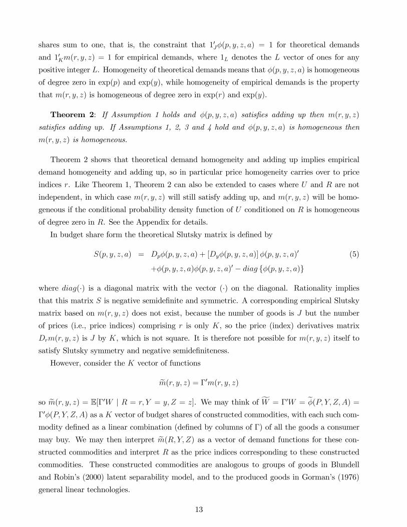
shares sum to one, that is, the constraint that 10J�(p; y; z; a) = 1 for theoretical demands

and 10Km(r; y; z) = 1 for empirical demands, where 1L denotes the L vector of ones for any

positive integer L. Homogeneity of theoretical demands means that �(p; y; z; a) is homogeneous

of degree zero in exp(p) and exp(y), while homogeneity of empirical demands is the property

that m(r; y; z) is homogeneous of degree zero in exp(r) and exp(y).

Theorem 2: If Assumption 1 holds and �(p; y; z; a) satis�es adding up then m(r; y; z)

satis�es adding up. If Assumptions 1, 2, 3 and 4 hold and �(p; y; z; a) is homogeneous then

m(r; y; z) is homogeneous.

Theorem 2 shows that theoretical demand homogeneity and adding up implies empirical

demand homogeneity and adding up, so in particular price homogeneity carries over to price

indices r. Like Theorem 1, Theorem 2 can also be extended to cases where U and R are not

independent, in which case m(r; y; z) will still satisfy adding up, and m(r; y; z) will be homo-

geneous if the conditional probability density function of U conditioned on R is homogeneous

of degree zero in R. See the Appendix for details.

In budget share form the theoretical Slutsky matrix is de�ned by

S(p; y; z; a) = Dp�(p; y; z; a) + [Dy�(p; y; z; a)]�(p; y; z; a)0 (5)

+�(p; y; z; a)�(p; y; z; a)0 � diag f�(p; y; z; a)g

where diag(�) is a diagonal matrix with the vector (�) on the diagonal. Rationality impliesthat this matrix S is negative semide�nite and symmetric. A corresponding empirical Slutsky

matrix based on m(r; y; z) does not exist, because the number of goods is J but the number

of prices (i.e., price indices) comprising r is only K, so the price (index) derivatives matrix

Drm(r; y; z) is J by K, which is not square. It is therefore not possible for m(r; y; z) itself to

satisfy Slutsky symmetry and negative semide�niteness.

However, consider the K vector of functions

em(r; y; z) = �0m(r; y; z)so em(r; y; z) = E[�0W j R = r; Y = y; Z = z]. We may think of fW = �0W = e�(P; Y; Z;A) =�0�(P; Y; Z;A) as a K vector of budget shares of constructed commodities, with each such com-

modity de�ned as a linear combination (de�ned by columns of �) of all the goods a consumer

may buy. We may then interpret em(R; Y; Z) as a vector of demand functions for these con-structed commodities and interpret R as the price indices corresponding to these constructed

commodities. These constructed commodities are analogous to groups of goods in Blundell

and Robin�s (2000) latent separability model, and to the produced goods in Gorman�s (1976)

general linear technologies.

13

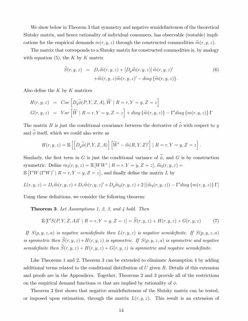
We show below in Theorem 3 that symmetry and negative semide�niteness of the theoretical

Slutsky matrix, and hence rationality of individual consumers, has observable (testable) impli-

cations for the empirical demands m(r; y; z) through the constructed commodities em(r; y; z).The matrix that corresponds to a Slutsky matrix for constructed commodities is, by analogy

with equation (5), the K by K matrix

eS(r; y; z) = Dr em(r; y; z) + [Dy em(r; y; z)] em(r; y; z)0 (6)

+em(r; y; z)em(r; y; z)0 � diag fem(r; y; z)g :Also de�ne the K by K matrices

H(r; y; z) = CovhDye�(P; Y; Z;A);fW j R = r; Y = y; Z = z

iG(r; y; z) = V ar

hfW j R = r; Y = y; Z = zi+ diag fem(r; y; z)g � �0diag fm(r; y; z)g�

The matrix H is just the conditional covariance between the derivative of e� with respect to yand e� itself, which we could also write as

H(r; y; z) = EhhDye�(P; Y; Z;A)i hfW 0 � em(R; Y; Z)0i j R = r; Y = y; Z = zi .

Similarly, the �rst term in G is just the conditional variance of e�, and G is by construction

symmetric. De�ne m2(r; y; z) = E [WW 0 j R = r; Y = y; Z = z], em2(r; y; z) =

E��0W (�0W )0 j R = r; Y = y; Z = z

�, and �nally de�ne the matrix L by

L(r; y; z) = Dr em(r; y; z)+Dr em(r; y; z)0+Dy em2(r; y; z)+2 [(em2(r; y; z))� �0diag fm(r; y; z)g�]

Using these de�nitions, we consider the following theorem:

Theorem 3: Let Assumptions 1, 2, 3, and 4 hold. Then

E [�0S(P; Y; Z;A)� j R = r; Y = y; Z = z] = eS(r; y; z) +H(r; y; z) +G(r; y; z) (7)

If S(p; y; z; a) is negative semide�nite then L(r; y; z) is negative semide�nite. If S(p; y; z; a)

is symmetric then eS(r; y; z)+H(r; y; z) is symmetric. If S(p; y; z; a) is symmetric and negativesemide�nite then eS(r; y; z) +H(r; y; z) +G(r; y; z) is symmetric and negative semide�nite.Like Theorems 1 and 2, Theorem 3 can be extended to eliminate Assumption 4 by adding

additional terms related to the conditional distribution of U given R. Details of this extension

and proofs are in the Appendices. Together, Theorems 2 and 3 provide all of the restrictions

on the empirical demand functions m that are implied by rationality of �.

Theorem 3 �rst shows that negative semide�niteness of the Slutsky matrix can be tested,

or imposed upon estimation, through the matrix L(r; y; z). This result is an extension of

14

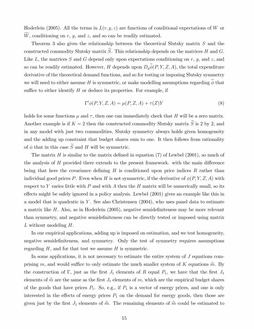
Hoderlein (2005). All the terms in L(r; y; z) are functions of conditional expectations of W orfW , conditioning on r, y, and z, and so can be readily estimated.Theorem 3 also gives the relationship between the theoretical Slutsky matrix S and the

constructed commodity Slutsky matrix eS. This relationship depends on the matrices H and G.

Like L, the matrices S and G depend only upon expectations conditioning on r, y, and z, and

so can be readily estimated. However, H depends upon Dye�(P; Y; Z;A), the total expenditure

derivative of the theoretical demand functions, and so for testing or imposing Slutsky symmetry

we will need to either assume H is symmetric, or make modelling assumptions regarding e� thatsu¢ ce to either identify H or deduce its properties. For example, if

�0�(P; Y; Z;A) = �(P;Z;A) + �(Z)Y (8)

holds for some functions � and � , then one can immediately check that H will be a zero matrix.

Another example is if K = 2 then the constructed commodity Slutsky matrix eS is 2 by 2, andin any model with just two commodities, Slutsky symmetry always holds given homogeneity

and the adding up constraint that budget shares sum to one. It then follows from rationality

of � that in this case eS and H will be symmetric.

The matrix H is similar to the matrix de�ned in equation (7) of Lewbel (2001), so much of

the analysis of H provided there extends to the present framework. with the main di¤erence

being that here the covariance de�ning H is conditioned upon price indices R rather than

individual good prices P . Even when H is not symmetric, if the derivative of �(P; Y; Z;A) with

respect to Y varies little with P and with A then the H matrix will be numerically small, so its

e¤ects might be safely ignored in a policy analysis. Lewbel (2001) gives an example like this in

a model that is quadratic in Y . See also Christensen (2004), who uses panel data to estimate

a matrix like H. Also, as in Hoderlein (2005), negative semide�niteness may be more relevant

than symmetry, and negative semide�niteness can be directly tested or imposed using matrix

L without modeling H.

In our empirical applications, adding up is imposed on estimation, and we test homogeneity,

negative semide�niteness, and symmetry. Only the test of symmetry requires assumptions

regarding H, and for that test we assume H is symmetric.

In some applications, it is not necessary to estimate the entire system of J equations com-

prising m, and would su¢ ce to only estimate the much smaller system of K equations em. Bythe construction of �, just as the �rst J1 elements of R equal P1, we have that the �rst J1elements of em are the same as the �rst J1 elements of m, which are the empirical budget shares

of the goods that have prices P1. So, e.g., if P1 is a vector of energy prices, and one is only

interested in the e¤ects of energy prices P1 on the demand for energy goods, then those are

given just by the �rst J1 elements of em. The remaining elements of em could be estimated to

15

test or impose Slutsky conditions, but that would still only require estimating K equations in

total rather than the much larger J . Note by Theorem 2 and the construction of �, em will

satisfy homogeneity if � satis�es homogeneity, so if � is rational and H is symmetric then emwill satisfy both homogeneity and Slutsky symmetry.

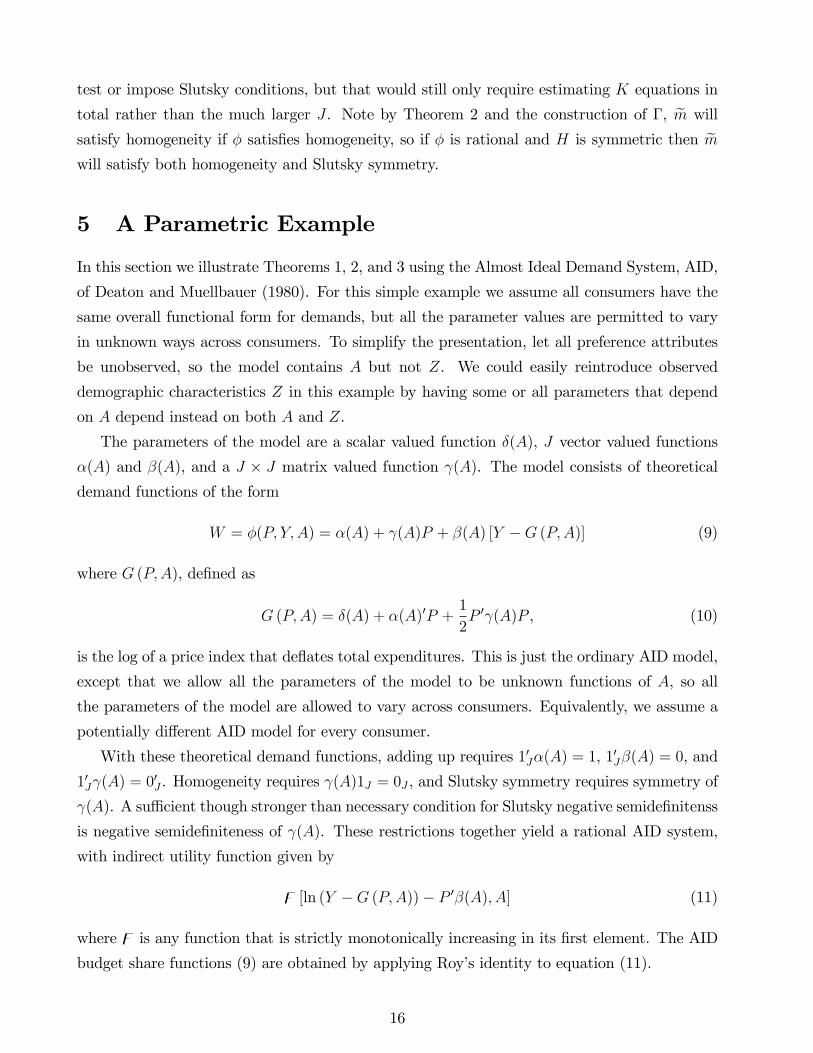
5 A Parametric Example

In this section we illustrate Theorems 1, 2, and 3 using the Almost Ideal Demand System, AID,

of Deaton and Muellbauer (1980). For this simple example we assume all consumers have the

same overall functional form for demands, but all the parameter values are permitted to vary

in unknown ways across consumers. To simplify the presentation, let all preference attributes

be unobserved, so the model contains A but not Z. We could easily reintroduce observed

demographic characteristics Z in this example by having some or all parameters that depend

on A depend instead on both A and Z.

The parameters of the model are a scalar valued function �(A), J vector valued functions

�(A) and �(A), and a J � J matrix valued function (A). The model consists of theoreticaldemand functions of the form

W = �(P; Y;A) = �(A) + (A)P + �(A) [Y �G (P;A)] (9)

where G (P;A), de�ned as

G (P;A) = �(A) + �(A)0P +1

2P 0 (A)P , (10)

is the log of a price index that de�ates total expenditures. This is just the ordinary AID model,

except that we allow all the parameters of the model to be unknown functions of A, so all

the parameters of the model are allowed to vary across consumers. Equivalently, we assume a

potentially di¤erent AID model for every consumer.

With these theoretical demand functions, adding up requires 10J�(A) = 1, 10J�(A) = 0, and

10J (A) = 00J . Homogeneity requires (A)1J = 0J , and Slutsky symmetry requires symmetry of

(A). A su¢ cient though stronger than necessary condition for Slutsky negative semide�nitenss

is negative semide�niteness of (A). These restrictions together yield a rational AID system,

with indirect utility function given by

z [ln (Y �G (P;A))� P 0�(A); A] (11)

where z is any function that is strictly monotonically increasing in its �rst element. The AIDbudget share functions (9) are obtained by applying Roy�s identity to equation (11).

16

Substituting equation P = �R + U into equation (9) gives

W = �(A) + (A)U + (A)�R + �(A) [Y �G(�R + U;A)] (12)

G(�R + U;A) = �(A) + �(A)0U +1

2U 0 (A)U + �(A)0�R + U 0 (A)�R +

1

2R0�0 (A)�R

Let Assumptions 1, 2, 3, and 4 hold with these rational theoretical demand functions, and

assume also that the covariances of �(A) with �(A), �(A), and (A) are all zero (more generally

if Z were present these would need to be zero conditional covariances conditioning on Z). This

will make the H matrix in Theorem 3 be zero. A su¢ cient though not necessary condition for

these covariances to equal zero is that �(A) not depend upon A. In this case H will equal zero

because equation (8) will hold.

With these assumptions, averaging equation (12) over U and A gives

W = m(R; Y ) + V (13)

where E(V j R; Y ) = 0J and

m(R; Y ) = �+ CR + b [Y � g (R)] (14)

g (R) = d+ a0�R +1

2R0�0CR (15)

Where d = E[�(A)] + E[�(A)]E(U) + 12E [U 0E[ (A)]U ], C = E[ (A)]�, b = E[�(A)], and

a = E[�(A)] + E[ (A)]E(U). The demand functions m(r; y), de�ned by substituting equation(15) into (14) could by equation (13) be estimated by, e.g., nonlinear least squares using ob-

served budget shares wit, log price indices rt, and log total expenditures yit from a collection of

(demographically homogeneous if we condition on Z) consumers i, each observed in one or more

time periods t, since, wit = m(rt; yit)+Vit. These demand functionsm(R; Y ) look similar to the

Almost Ideal (though with di¤erent parameter values from those of the individual consumers),

however, they are not quite Almost Ideal, because the number of prices (elements of R) is only

K while the number of budget shares (elements of m) is J , so C is J�K, not square like (A).Still, in this particular parametric example we obtain the nearly linear AID like model

W = a + CR + beY + V where eY equals log de�ated total expenditures Y � g (R). This looksjust like an ordinary aggregate AID model, except that instead of regressing each element ofW

on a constant, eY , and all J prices P , we obtain the coe¢ cients a, b, and C by just regressingeach element of W on a constant, eY , and the K price indices R, which include the prices of

interest P1 = R1.

In the model of equations (13), (14), and (15) adding up requires 10Ja = 1, 10Jb = 0, and

10JC = 00J . This can be obtained in the usual way by omitting one good, and using these

adding up constraints to obtain the parameters corresponding to the last good. Homogeneity

17

requires in addition that C1K = 0J , and Slutsky symmetry requires symmetry not of C (which

is impossible because C is not square), but of �0C. Also, if (A) is negative semide�nite then

�0C will be semide�nite.

6 An Aggregate Empirical Example: Gasoline Prices

As a �rst empirical illustration of the methodology, we aggregate the parametric AID based

model of the previous section across consumers in each time period, and estimate the resulting

model using total United States consumption data to assess the impact of gasoline prices on

the demands for a large number of consumer goods.

From tables 2.4.5 and 2.4.6 of the US National Income and Product Accounts (NIPA) we

obtain budget shares Wjt and associated logged prices (consumption de�ators) Pjt for J = 22

di¤erent goods j for 45 years t from 1960 to 2004. The logged prices Pjt are demeaned over

time (this corresponds to a particular choice of units for measuring quantities of each good)

so principal components can be easily used for constructing price indices. Speci�cally, we let

R1t = P1t be the logged price of gasoline in time t, and we then de�ne R2, the last J2 elements

of R, as follows. Let Sit be the i0th principal component of the matrix of P2 consisting of all

logged prices except gasoline. Then by construction Sit = P2t�i where �i is a 21 element vector

of weights. The corresponding logged price index Ri+1;t for i = 1, 2, and 3 is then de�ned by

Ri+1;t = P 02t�i=(1021�i) where 121 denotes the vector of 21 ones. This scaling of the principal

component is necessary to ensure that R satis�es the homogeneity property of price indices

(e.g., if all prices exp(P ) double then the price indices exp(R) must also double).

We then de�ne � and Ut by Pt = �Rt+Ut where the j�th row of � consists of the coe¢ cients

from a constrained linear time series regression of Pjt on the four elements of Rt, and we de�ne

Ujt (the j�th element of Ut for each t) as the time t residual from this regression. Assumption 2

requires the rows of � to sum to one, so this constraint is imposed on the regressions de�ning

each row of �.

The AID model is quadratic in logged prices (through the function g), so for this model

Assumption 4 can be relaxed to only require that the conditional mean and variance of U

given R be independent of R. Since U is de�ned as a set of regression residuals, U is by

construction uncorrelated with R. To check the variance condition, we apply a White (1980)

test for heteroskedasticity to each of the above price regressions. Table 1 gives the estimates of

�, along with the R2�s of these regressions and the White test statistics.

To apply the model of the previous section to total US consumption data, we must aggregate

this model across consumers in each time period. By equations (13), (14), and (15), we may

write the budget shares for individual consumers (households) h in time t as Wht = At +

18

b lnXht + Vht, where Xht is total expenditures and At = a+ Crt � bg (Rt). Total expendituresfor each good are therefore given by XhtWht = AtXht+ bXht lnXht+VhtXht, and averaging this

expression across all consumers in time t then gives aggregate (per capita) budget shares

Wt =Et(XhtWht)

Xt

= At + bEt(Xht lnXht)

Xt

+ Vt

where Et denotes averaging across households h in time t, with Xt = Et(Xht). This notation

means that Xht equals an Xt that varies randomly over time, plus a random term that for

any time period t is mean zero across households h. Here Xt = Et(Xht) is per capita total

expenditures in time period t and Vt = Et(VhtXht)=Xt is an aggregate error term.

Lewbel (1991) showed that in the U.S. using income, Et(Xht lnXht) � Xt�+Xt lnXt, where

� is a constant. In particular, he �nds that a linear time series regression of Et(Xht lnXht) on

Xt and Xt lnXt, imposing a coe¢ cient of one on the latter term, has an R2 over .998, so roughly

the approximation error here is less than .2 percent. Substituting this approximation into the

above expression forWt then givesWt = (At+b�)+b lnXt+Vt, where Vt now includes this small

approximation error resulting from aggregation across Xht. The resulting model we estimate is

then

Wt = a+ CRt + b [lnXt � g (Rt)] + Vt (16)

g (Rt) = d+ a0�Rt +1

2R0t�

0CRt (17)

where d = d + �. As with ordinary AID model estimation, the constant d is underidenti�ed

and so is set to zero.

We estimate this aggregate, macro data model using budget sharesWt constructed as NIPA

consumption expenditures on each good j divided by the sum of these expenditures across all

goods, and per capita total expenditures Xt de�ned as this sum of NIPA expenditures across

all goods, divided by US population. To avoid separability assumptions, our list of goods

includes durables as well as nondurables and services. We do not attempt to construct �ows of

services derived from durables, noting that aggregation across consumers smooths out most of

the lumpiness in durable consumption that results from infrequency of purchase.

By analogy with the common approximate AID model, we �rst linearly regress Wt on a

constant, Rt, and on lnXt � P 0tWt. This is not a consistent estimator, but yields reasonable

starting values ba, bb, and bC for our formal estimator. We estimate equation (16) using three

stage least squares (speci�cally, GMM with a weighting matrix that is is e¢ cient under ho-

moskedasticity, which for large systems like ours can have good �nite sample properties and

fewer numerical convergence problems than general e¢ cient GMM. See e.g., Wooldridge 2002

for details). Estimation is based on the moment conditions

E��Wt � a� CRt � b

�lnXt � a0�Rt �

1

2R0t�

0CRt

��Qst

�= 0J , s = 1; :::; S

19

where the set of S instruments Q1t,...,QSt consists of a constant, lnXt, all K = 4 elements of

Rt, a time trend t, and R0t�0 bCRt using the above starting value of bC. Note that estimation

error in bC only a¤ects e¢ ciency but not consistency of the resulting three stage least squaresestimator, because R0t�

0 eCRt is a valid instrument (in the sense of being uncorrelated with themodel error) for any choice of the matrix eC. We could more generally use any functions of Xt

and Rt as instruments, but this set works well numerically in our small sample, because the

model is nearly linear in Q1t,...,QSt.

We impose the adding up constraints by omitting one good from the system. We estimate the

model without the homogeneity and Slutsky symmetry restrictions C1K = 0J and �0C = C 0�,

so these restrictions can be tested. Wald tests of these restrictions are reported in Table 2, while

Table 3 reports results of testing homogeneity separately in each of the twenty two separate

demand equations. As is often the case with aggregate data, overall symmetry is rejected, and

for most but not all goods homogeneity is also rejected (though see the caveats below regarding

possible statistical invalidity of these tests). Far fewer rejections are obtained with individual

consumer data in the next section.

Table 4 reports Cj1 for each equation j, which is the estimated derivative of the budget share

of good j with respect to the logged price of gasoline, holding de�ated log total expenditures

lnxt� g (rt) �xed. Table 4 also reports bj for each good j, which is the estimated derivative ofthe budget share of good j with respect to log total expenditures. Standard errors are provided

in parentheses.

Most empirical implementations of demand system models do not adjust standard errors to

account for price index estimation. Errors in demand systems are typically rather large (due

to substantial unobserved heterogeneity of preferences), so the additional contribution to the

�nal standard errors of �rst stage estimation of price indices is likely to be relatively modest.

Still, since our aggregate model is completely parametric, to account for estimation error in the

construction of price indices R and to account for any autocorrelation in the residuals, we also

estimated con�dence intervals for these parameters using an ordinary block bootstrap. In this

bootstrap consecutive time blocks of the original data are drawn with replacement, which are

then used to construct price indices, estimate the model, and construct parameter t-statistics.

We construct 95% con�dence intervals across the bootstrap simulations for these t statistics,

and convert the results back into con�dence intervals for the underlying parameters. Due to

the small sample size of n = 45, we picked rather small blocks of size 4. Still, we had to discard

some bootstrap simulations that experienced severe colinearity issues resulting in a singular

or ill-conditioned variance covariance matrix. Attempts to bootstrap with larger block sizes

produced a higher percentage of numerical failures of this type. This points to the limits of

attempting sophisticated asymptotic analyses in this speci�c small sample application.

20

Table 5 provides the mean of each budget shareWj in the data, and reports the correspond-

ing estimates of the elasticity (at the mean) of quantity demands with respect to gasoline prices

and with respect to total expenditures. These are immediately obtained from the derivative

estimates and the budget share means. For comparative convenience this table includes the

derivative estimates from Table 4 that are used to construct the reported elasticities.

The total expenditure elasticities are for the most part quite sensible. Durables generally

have high expenditure elasticities as would be expected since consumers can adjust the timing of

their purchases of durables to when their incomes are relatively high. The gasoline expenditure

elasticity is unexpectedly high, though the corresponding total expenditure derivative is not

signi�cantly di¤erent from zero.

The own price elasticity for gasoline, -.87 is negative, inelastic, and statistically signi�cant.

Recall a novel feature of the methodology is that it provides detailed cross price e¤ects, and in

this application these are the separate e¤ects of gasoline prices on every other good consumer�s

purchase. Of course most of these cross e¤ects are small or insigni�cant, but some are quite

interesting. For example, we �nd when gasoline prices increase one percent, the demand for

transportation other than personal car use (planes, trains, buses, etc.,) goes up .06 percent,

which is useful information for analyzing gasoline tax e¤ects and responses to oil shocks.

To check for possible simultaneity with supply we experimented with reestimating the model

replacing Rt in the construction of the instruments Zst with some of the same supply side

variables used for that purpose by Lewbel and Ng (2005) and Jorgenson, Lau, and Stoker

(1982). We do not report these results because they did not change the overall conclusions

in any substantial way, and to maintain greater consistency with our price aggregation theory

(particularly assumption 3i).

Overall, our aggregate data results illustrate the feasibility of using our methodology to

estimate demand systems with large numbers of equations and goods. We consider this ap-

plication to be an extreme test of the methodology because our data consists of only 45 time

periods, so obtaining any kind of reasonable estimates in a model with 22 goods and no imposed

separability seems like a success. Still, these results come with numerous caveats. Estimation

of such a large model with relatively few observations means that our asymptotic standard

errors, hypothesis tests, and bootstrap con�dence intervals likely su¤er from relatively large

biases associated with small samples.

We have not dealt with possible nonstationarity of prices. As noted earlier, nonstationarity

helps to satisfy our price aggregation assumptions, to the extent that it makes variation in U

small relative to variation in R (as seen in the generally high R2 statistics in Table 1). However,

nonstationarity of regressors in nonlinear models invalidates the standard asymptotic limiting

distribution theory underlying our hypothesis tests. Little is known about the distribution of

21

nonlinear model parameter estimates with nonstationary data in general, though see Lewbel

and Ng (2005) for a demand system functional form that can be estimated with nonstationary

price data. Finally, both our parametric functional form and the aggregation across consumers

impose strong restrictions that may not be valid empirically. These we relax in our next

application.

7 Nonparametric Estimation and Testing

The estimates presented in the previous section depended on many restrictive, parametric

modelling assumptions. In this section we work with consumption data from a relatively ho-

mogeneous sample of individual households. The resulting elasticity estimates therefore have

less general policy relevance than the previous macro estimates, but these data permit direct

nonparametric estimation of elasticities and testing. In particular, we can directly estimate the

functions m(r; y; z) by nonparametric regressions of w on r; y; z, and nonparametrically test if

they are homogeneous and if the corresponding Slutsky related matrix eS(r; y; z) is symmetricand negative semide�nite.

The data are observations of expenditures, demographic composition, and other characteris-

tics of a demographically relatively homogeneous set of households drawn from the years 1974 to

1993 of the british family expenditure survey (FES). The sample consist of about 7,000 house-

holds, all consisting of childless couples with at least one employed member and with the head

of the household being a white collar worker. To account for remaining observable demographic

heterogeneity in a nonparametrically tractable way, we include a covariate Z constructed as the

�rst principal component of the the remaining demographic household characteristics reported

in the FES. The expenditures of all goods are grouped into twelve categories, which are Food,

Catering, Alcohol, Tobacco, Housing, Household Goods, Household Services, Clothing, Motor-

ing, Fares, Leisure Services and Gasoline. We construct R to be three dimensional, with �rst

element being the log price of gasoline as before, and the second two elements as the suitably

scaled �rst two principal component of the log price indices of the remaining eleven goods, using

the same scaling procedure as with the aggregate data example. We also construct � using the

same procedure as with the aggregate data. We experimented with including more price and

demographic components, but these caused problems associated with the nonparametric curse

of dimensionality

We nonparametrically estimate the demand functions m(r; y; z) using kernel based local

polynomial regressions and apply bootstrap methods to obtain critical values for hypothesis test

statistics as in Hoderlein (2005) and Haag, Hoderlein, and Pendakur (2009), so refer to those

papers for associated econometric distribution theory and details. The principal components R

22

are estimated at a parametric rate, and m(r; y; z) is a smooth function of r, so by a standard

Taylor expansion of the estimated m around the true R, one may readily show that (as usual

for a parametric generated regressor in a nonparametric regression) estimation error in R is to

�rst order asymptotically irrelevant for estimation of m.

Endogeneity of total expenditure could be an issue, so we estimate the model a second time

allowing for endogeneity of y by using labor income as an instrument and including correspond-

ing control function residuals in the nonparametric regressions as in Newey, Powell, and Vella

(1999). With this household level data we do not instrument prices, both for consistency with

our formal assumptions (particularly Assumption 3i) and because the contribution of any one

consumer�s demands (or even all consumers in the subset of the population we sample from) to

aggregate demand, and hence to price determination, should be small.

Table 7 reports the mean elasticity of each budget share with respect to gasoline prices

and with respect to total expenditures, along with bootstrapped 95% con�dence intervals. The

results show similar patterns to the aggregate data, such as high total expenditure elasticities

for durables. Gasoline demand itself has almost the same own price elasticity as in the aggregate

data, and shows many similar cross price e¤ects (again including a small positive cross e¤ect

on other transportation), though these nonparametric cross price e¤ects are not estimated with

enough precision to be statistically signi�cant.

Table 8 lists results of various tests of rationality restrictions. We evaluate the estimated

nonparametric demand functions and their derivatives at each data point, and for each ob-

servation we test whether the demand functions at that point satisfy homogeneity, negative

semide�niteness, and Slutsky symmetry. For each hypothesis, Table 8 lists the percent of

observations at which the hypothesis is not rejected at the 0.95 con�dence level.

Table 8 shows that homogeneity (the absence of money illusion) is generally accepted,

with a rejection rate of 11% of the data when we allow for endogenous regressors. We test

symmetry and negative semide�niteness of the composite commodity Slutsky matrix eS(r; y; z)both with and without imposing homogeneity. Note that imposing homogeneity speeds the

rate of convergence by reducing dimensionality (see, e.g., Tripathi and Kim 2001). We reject

symmetry and negative semide�niteness in 13% to 26%, depending on whether or not we impose

homogeneity or allow for endogeneity.

Overall, we �nd that our method of handling price multicollinearity through price dimension

reduction yields reasonable nonparametric demand model estimates that are usually consistent

with consumer rationality. The somewhat lower acceptance rates for symmetry versus homo-

geneity could be due to the fact that symmetry involves a greater number of restrictions, or

some couples might employ bargaining or other non social welfare maximizing expenditure

allocation schemes that yield symmetry violations of the unitary model as in Browning and

23

Chiappori (1998)

8 Conclusions

We have shown how demand systems can be estimated, with rationality imposed, while replac-

ing the complete set of prices of all goods with a small set of prices of interest and a few summary

price indices. We illustrate the results by reporting estimates of the e¤ects of gasoline prices on

the demands for many goods, both with an aggregate data parametric model to obtain some

macroeconomic elasticities, and nonparametrically for a demographically homogeneous sample

of individual households. The methodology is easy to implement either in parametric demand

models or using ordinary nonparametric regressions.

In parametric models, this dimension reduction mitigates problems of multicollinearity of

prices. In our parametric model, we replace J equals twenty two separate prices with K equals

four price aggregates. The gains from reducing dimensionality of prices in the nonparametric

context are more dramatic. In our nonparametric application we have J equals twelve prices

that we reduce to K equals three price aggregates, along with a demographic and a total ex-

penditures variable. Our methodology therefore reduces the dimension of these nonparametric

demand function regressions from fourteen to �ve regressors, which yields an enormous increase

in rates of convergence without behavioral demand function restrictions.

More generally, we have shown how statistical dimension reduction techniques can be ap-

plied in optimizing models arising from microeconomic theory, which have multiple nonlinear

equations, nonseparable unobservables, nonlinear cross equation restrictions, and many poten-

tially multicollinear covariates.

References

[1] Berry, S., J. Levinsohn, and A. Pakes (1995), "Automobile Prices in Market Equilibrium,"

Econometrica, 841-890.

[2] Blackorby, Charles, Daniel Primont, and R. Robert Russell (1978), Duality, Separability,

and Functional Structure: Theory and Economic Applications, North-Holland: New York.

[3] Blundell, Richard and Jean Marc Robin (2000), "Latent Separability: Grouping Goods

without Weak Separability, Econometrica, 68, pp. 53-84.

[4] Brown, R. and M. Walker, (1989), "The Random Utility Hypothesis and Inference in

Demand Systems", Econometrica, 57, pp. 815-829.

24

[5] Browning, Martin, and Pierre-Andre Chiappori, (1998) "E¢ cient Intra-Household Alloca-

tions: A General Characterization and Empirical Tests," Econometrica, 66, 1241-1278.

[6] Christensen, Mette (2004), "Integrability of Demand Accounting for Unobservable Hetero-

geneity: A Test on Panel Data," unpublished manuscript.

[7] Davis, George C. �The Generalized Composite Commodity Theorem: Stronger Support

in the Presence of Data Limitations.�Review of Economics and Statistics, 85, 476�480.

[8] Deaton, Angus (1975), Models and Projections of Demand in Post-War Britain, London:

Chapman and Hall.

[9] Deaton, Angus, and John Muellbauer, (1980), An almost ideal Demand System, American

Economic Review, pp. 312-26.

[10] Diewert, Walter Erwin, (1974), �Applications of Duality Theory,�in: Frontiers of Quan-

titative Economics, vol. II, M.D. Intriligator and D. A. Kendrick, eds., North-Holland:

Amsterdam, pp. 106-171.

[11] Gorman, William M. (1959), "Separable Utility and Aggregation," Econometrica, 27, 469-

481.

[12] Gorman, William M. (1976), �Tricks With Utility Functions,� In Essays in Economic

Analysis: Proceedings of the 1975 AUTE Conference, She¢ eld, edited by M. J. Artis and

A.R. Nobay, pp. 211-243.

[13] Haag, Berthold, Hoderlein, Stefan and Krishna Pendakur (2009), "Testing and Imposing

Slutsky Symmetry in Nonparametric Demand Systems,"Journal of Econometrics, forth-

coming..

[14] Hicks, John R. (1936), Value and Capital, Oxford: Oxford University Press.

[15] Hoderlein, Stefan, (2005), "Nonparametric Demand Systems, Instrumental Variables and

a Heterogeneous Population," unpublished manuscript, Brown University.

[16] Judge, G.G., Gri¢ ths, W.E., Hill, R.C., Lütkepohl, H. and Lee, T. (1985), "The Theory

and Practice of Econometrics", second edition, John Wiley & Sons.

[17] Leontief, Wassily (1936), "Composite Commodities and the Problem of Index Numbers."

Econometrica, 4, 39-59.

25

[18] Lewbel, Arthur (1991), �The Rank of Demand Systems: Theory and Nonparametric Esti-

mation,�Econometrica, 59, 711-730.

[19] Lewbel, Arthur, (1996), "Aggregation Without Separability: A Generalized Composite

Commodity Theorem," American Economic Review, 86, pp. 524-543.

[20] Lewbel, Arthur, (2001), �Demand Systems with and without Errors�, American Economic

Review, pp. 611-18.

[21] Lewbel, Arthur and Serena Ng, (2005), "Demand Systems With Nonstationary Prices,"

Review of Economics and Statistics, pp. 479 - 494.

[22] Newey, Whitney K., James L. Powell, and Frank Vella (1999), �Nonparametric Estimation

of Triangular Simultaneous Equations Models�, Econometrica, 67, 567�603.

[23] Pendakur, Krishna, (1999), �Estimates and Tests of Base-Independent Equivalence Scales�

Journal of Econometrics, 88, 1-40.

[24] Tripathi, Gautam, and Woocheol. Kim, (2003), "Nonparametric estimation of homoge-

neous function," Econometric Theory, 19, 640-663.

[25] White, Halbert (1980), "Heteroskedasticity-Consistent Covariance Matrix Estimator and

a Direct test for Heteroskedasticity", Econometrica, pp. 817-836.

[26] Wooldridge, Je¤rey M. (2002), Econometric Analysis of Cross Section and Panel Data,

Cambridge: MIT Press.

Appendix I: Technical Assumptions and Extensions

To allow dependence of U on R we now consider replacing Assumption 4 with the following.

Assumption 5: The conditional distribution of U2 given R = r is continuous, with condi-

tional probability density function fU2jR(U2 j r) that is di¤erentiable in r.

We then obtain Theorems 10 20 and 30 below, which extend Theorems 1, 2 and 3, respectively.

Generally speaking, the e¤ect of Assumption 5 in place of Assumption 4 is to add additional

terms that depend upon the conditional density of U2.

Theorem 10: Let Assumptions 1, 2, 3, and 5 hold. Then

Drm(r; y; z) = E�Dp�(P; Y; Z;A)� +WDr log fU2jR(U2 j R) j R = r; Y = y; Z = z

�. (18)

26

We introduce the notation Cor(r; y; z) = ��0E�WDr log fU2jR(U2 j R) j R = r; Y = y; Z = z

�:

Theorem 20: Let Assumptions 1, 2, 3 and 5 hold. If �(p; y; z; a) satis�es adding up then

m(r; y; z) satis�es adding up. If �(p; y; z; a) is homogeneous and fU2jR(U2 j r) = fU2jR(U2 jr + �) for any scalar � then m(r; y; z) is homogeneous.

Theorem 20 requires that the conditional density of the errors U in the price dimension re-

duction equation be homogeneous of degree zero in the price indices exp(R). This is empirically

testable in a variety of ways, e.g., one could directly apply general nonparametric speci�cation

tests to test the hypothesis that fU2jR(U2 j R) equal the conditional density of U2 just condi-tioning on R�RJ where RJ is the last element of R. This test would use a parametric estimateof U2 and kernel estimates of the required conditional densities.

An implication of this density homogeneity is that the conditional variance of U given R is

homogeneous. A simple parametric test of the hypothesis would be to regress U2U 02 on R�RJand RJ , and test if the coe¢ cients on RJ are insigni�cant.

Theorem 30: Let Assumptions 1, 2, 3 and 5 hold. Assume fU2jR(U2 j r) is di¤erentiable inr. Then

E [�0S(P; Y; Z;A)� j R = r; Y = y; Z = z] = eS(r; y; z) +H(r; y; z) +G(r; y; z) + Cor(r; y; z):(19)

Therefore, if S(p; y; z; a) is negative semide�nite then eS(r; y; z) + H(r; y; z) + G(r; y; z) +Cor(r; y; z) is negative semide�nite and if S(p; y; z; a) is symmetric then eS(r; y; z)+H(r; y; z)+Cor(r; y; z) is symmetric. In addition, if S is negative semide�nite then

Dr em(r; y; z) + �0 fDym2(r; y; z) + 2(m2(r; y; z))g�� diag fem(r; y; z)g+ Cor(r; y; z)is negative semide�nite.

Appendix II: Proofs and Tables

Proof of Theorems 1 and 10: By boundedness of W the expectation of W exists, and

therefore also the conditional expectation

m(r; y; z) = E [�(P; Y; Z;A) j R = r; Y = y; Z = z]

=

ZA�U2

�(�b+ u; y; z; a)FU2;AjR;Y;Z(du2; da j r; y; z)

Note that the �rst K elements of u are zero by construction, and the remaining elements are u2.

By Assumption 3(i), we may separate the integration over U and R from the (A; Y; Z), and we

27

may use the conditional independence of A from Y to drop y from the conditional distribution

of A. Summarizing, we obtain

m(r; y; z) =

ZA

�ZU2�(�r + u; y; z; a)fU2jR(u2 j r)du2

�FAjZ(da j z). (20)

For Theorem 1, replace fU2jR(u2 j r)du2 with FU2(du2) in the above expression. Equation (2)follows immediately by taking the derivative of equation (20) with respect to y; and interchang-

ing di¤erentiation and integration, given bounded convergence. Finally, taking the derivative

with respect to r gives

Drm(r; y; z) =

ZA

�ZU2Dr

��(�r + u; y; z; a)fU2jR(u2 j r)

�du2

�FAjZ(da j z);

and

Dr

��(�r + u; y; z; a)fU2jR(u2 j r)

�= Dp�(p; y; z; a)�fU2jR(u2 j r) + �(p; y; z; a)DrfU2jR(u2 j r)

=�Dp�(p; y; z; a)� + �(p; y; z; a)DrfU2jR(u2 j r)

�fU2jR(u2 j r);

which gives equation (18). The same derivation replacing fU2jR(u2 j r)du2 with FU2(du2) makesthe second term in this expression be zero, yielding equation (4). Equation (3) follows from

equation (4) given r1 = p1 and the structure of �.

Proof of Theorems 2 and 20: Adding a constant � to each element of r in equation (20)

gives

m(r + �; y; z) =

ZA

�ZU2�(�r + u+ �1K�; y; z; a)fU2jR(u2 j r + �)du2

�FAjZ(da j z):

Now �1K = 1J so �(�r + u+ �1K�; y; z; a) = �(�r + u; y; z; a) if �(p+ �; y; z; a) = �(p; y; z; a)

and so if we also have either fU2jR(u2 j r + �) = fU2jR(u2 j r) or if fU2jR(u2 j r) is replaced withFU2(du2), then m(r + �; y; z) = m(r; y; z).

Proof of Theorem 3 and Theorem 30: For compactness of notation, let condition-

ing on r; y; z denote conditioning on the event R = r; Y = y; Z = z. De�ne ~�(P; Y; Z;A) =

�0�(P; Y; Z;A). Dropping the argument (P; Y; Z;A) from � and ~� for clarity we have em(r; y; z) =Ehe� j r; y; zi. Multiplying equation (2) in Theorem 1 by �0 givesDy em(r; y; z) = �0Dym(r; y; z) =

�0E [Dy� j r; y; z] = E [Dy (�0�) j r; y; z] = E

hDye� j r; y; zi. Similarly, multiplying equation (4)

in Theorem 1 by �0 gives Dr em(r; y; z) = �0Drm(r; y; z) = �0E [Dp� j R = r; Y = y; Z = z] �.Substituting these into the de�nition of eS(r; y; z) gives

eS(r; y; z) = �0E [Dp� j r; y; z] � + EhDye� j r; y; ziE he� j r; y; zi0 +

Ehe� j r; y; ziE he� j r; y; zi0 � diag nE he� j r; y; zio

28

Now by the de�nition of the Slutsky matrix S we have

E [�0S� j r; y; z] = �0E [Dp� j r; y; z] �

+E [(Dy (�0�)) (�0�) + �0��0�� �0diag f�g� j r; y; z]

= �0E [Dp� j r; y; z] � + Eh�Dye�� e�0 j r; y; zi

+Ehe�e�0 j r; y; zi� �0diag fE [� j r; y; z]g�

So

E [�0S� j r; y; z]� S(r; y; z) = CovhDye�; e�0 j r; y; zi+ V ar he� j r; y; zi

+diagnE[e� j r; y; z]o� �0diag fE [� j r; y; z]g�

Which gives equation (7). Semide�niteness and symmetry of S imply semide�niteness and

symmetry of E [�0S� j r; y; z], which given (7) and symmetry ofG proves the rest of the theorem.The proof of theorem 3 follows exactly be the same arguments, including the correction term

as in theorem 10.

Finally, to see the last statement in Theorem 3�(regarding the matrix L in Theorem 3),

note that semide�niteness of S implies semide�niteness of of E [�0 (S + S 0) � j r; y; z]. Next,note that

E [�0 (Dy��0 + �Dy�

0) � j r; y; z] = �0DyE [WW 0 j r; y; z] � = Dy em2 (r; y; z) ;

where we used again the conditional independence of A and Y for the �rst equality. The result

follows by collecting terms and noticing that the last two terms are symmetric.

29

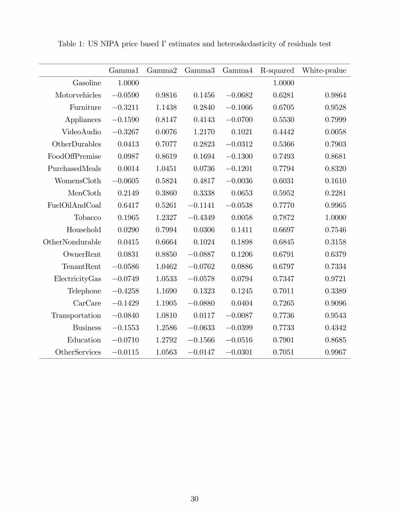
Table 1: US NIPA price based � estimates and heteroskedasticity of residuals test

Gamma1 Gamma2 Gamma3 Gamma4 R-squared White-pvalue

Gasoline 1.0000 1.0000

Motorvehicles �0.0590 0.9816 0.1456 �0.0682 0.6281 0.9864

Furniture �0.3211 1.1438 0.2840 �0.1066 0.6705 0.9528

Appliances �0.1590 0.8147 0.4143 �0.0700 0.5530 0.7999

VideoAudio �0.3267 0.0076 1.2170 0.1021 0.4442 0.0058

OtherDurables 0.0413 0.7077 0.2823 �0.0312 0.5366 0.7903

FoodO¤Premise 0.0987 0.8619 0.1694 �0.1300 0.7493 0.8681

PurchasedMeals 0.0014 1.0451 0.0736 �0.1201 0.7794 0.8320

WomensCloth �0.0605 0.5824 0.4817 �0.0036 0.6031 0.1610

MenCloth 0.2149 0.3860 0.3338 0.0653 0.5952 0.2281

FuelOilAndCoal 0.6417 0.5261 �0.1141 �0.0538 0.7770 0.9965

Tobacco 0.1965 1.2327 �0.4349 0.0058 0.7872 1.0000

Household 0.0290 0.7994 0.0306 0.1411 0.6697 0.7546

OtherNondurable 0.0415 0.6664 0.1024 0.1898 0.6845 0.3158

OwnerRent 0.0831 0.8850 �0.0887 0.1206 0.6791 0.6379

TenantRent �0.0586 1.0462 �0.0762 0.0886 0.6797 0.7334

ElectricityGas �0.0749 1.0533 �0.0578 0.0794 0.7347 0.9721

Telephone �0.4258 1.1690 0.1323 0.1245 0.7011 0.3389

CarCare �0.1429 1.1905 �0.0880 0.0404 0.7265 0.9096

Transportation �0.0840 1.0810 0.0117 �0.0087 0.7736 0.9543

Business �0.1553 1.2586 �0.0633 �0.0399 0.7733 0.4342

Education �0.0710 1.2792 �0.1566 �0.0516 0.7901 0.8685

OtherServices �0.0115 1.0563 �0.0147 �0.0301 0.7051 0.9967

30

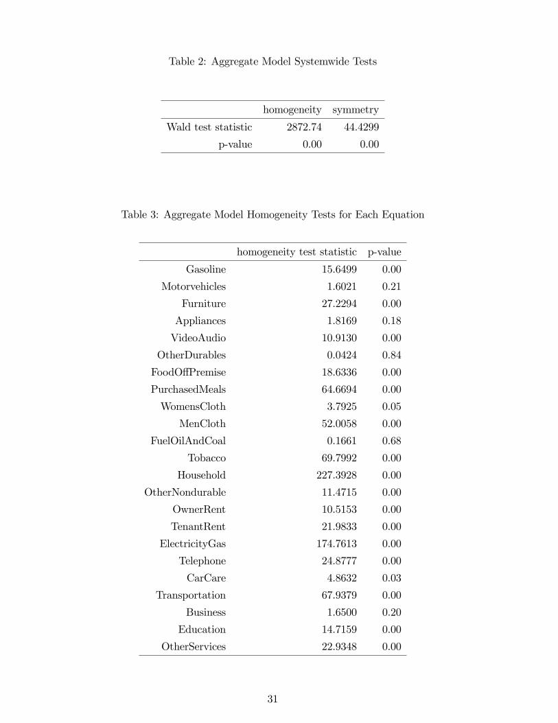
Table 2: Aggregate Model Systemwide Tests

homogeneity symmetry

Wald test statistic 2872.74 44.4299

p-value 0.00 0.00

Table 3: Aggregate Model Homogeneity Tests for Each Equation

homogeneity test statistic p-value

Gasoline 15.6499 0.00

Motorvehicles 1.6021 0.21

Furniture 27.2294 0.00

Appliances 1.8169 0.18

VideoAudio 10.9130 0.00

OtherDurables 0.0424 0.84

FoodO¤Premise 18.6336 0.00

PurchasedMeals 64.6694 0.00

WomensCloth 3.7925 0.05

MenCloth 52.0058 0.00

FuelOilAndCoal 0.1661 0.68

Tobacco 69.7992 0.00

Household 227.3928 0.00

OtherNondurable 11.4715 0.00

OwnerRent 10.5153 0.00

TenantRent 21.9833 0.00

ElectricityGas 174.7613 0.00

Telephone 24.8777 0.00

CarCare 4.8632 0.03

Transportation 67.9379 0.00

Business 1.6500 0.20

Education 14.7159 0.00

OtherServices 22.9348 0.00

31

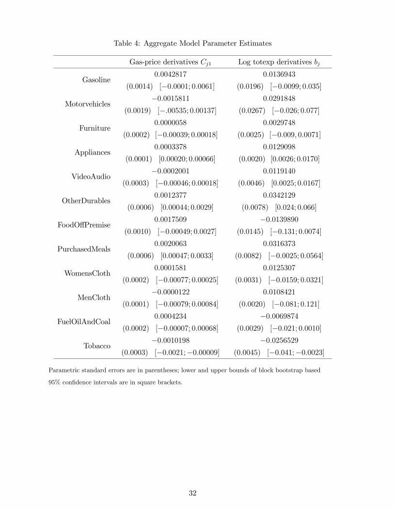
Table 4: Aggregate Model Parameter Estimates

Gas-price derivatives Cj1 Log totexp derivatives bj

Gasoline0:0042817

(0:0014) [�0:0001; 0:0061]0:0136943

(0:0196) [�0:0099; 0:035]

Motorvehicles�0:0015811

(0:0019) [�:00535; 0:00137]0:0291848

(0:0267) [�0:026; 0:077]

Furniture0:0000058

(0:0002) [�0:00039; 0:00018]0:0029748

(0:0025) [�0:009; 0:0071]

Appliances0:0003378

(0:0001) [0:00020; 0:00066]

0:0129098

(0:0020) [0:0026; 0:0170]

VideoAudio�0:0002001

(0:0003) [�0:00046; 0:00018]0:0119140

(0:0046) [0:0025; 0:0167]

OtherDurables0:0012377

(0:0006) [0:00044; 0:0029]

0:0342129

(0:0078) [0:024; 0:066]

FoodO¤Premise0:0017509

(0:0010) [�0:00049; 0:0027]�0:0139890

(0:0145) [�0:131; 0:0074]

PurchasedMeals0:0020063

(0:0006) [0:00047; 0:0033]

0:0316373

(0:0082) [�0:0025; 0:0564]

WomensCloth0:0001581

(0:0002) [�0:00077; 0:00025]0:0125307

(0:0031) [�0:0159; 0:0321]

MenCloth�0:0000122

(0:0001) [�0:00079; 0:00084]0:0108421

(0:0020) [�0:081; 0:121]

FuelOilAndCoal0:0004234

(0:0002) [�0:00007; 0:00068]�0:0069874

(0:0029) [�0:021; 0:0010]

Tobacco�0:0010198

(0:0003) [�0:0021;�0:00009]�0:0256529

(0:0045) [�0:041;�0:0023]

Parametric standard errors are in parentheses; lower and upper bounds of block bootstrap based

95% con�dence intervals are in square brackets.

32

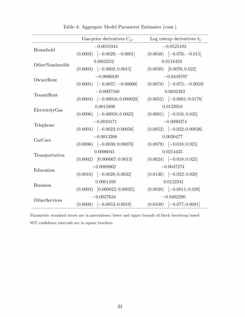
Table 4: Aggregate Model Parameter Estimates (cont.)

Gas-price derivatives Cj1 Log totexp derivatives bj

Household�0:0010344

(0:0003) [�0:0029;�0:0001]�0:0525102

(0:0048) [�0:076;�0:015]

OtherNondurable0:0002252

(0:0003) [�0:0002; 0:0013]0:0118459

(0:0039) [0:0076; 0:022]

OwnerRent�0:0006820

(0:0005) [�0:0037;�0:00006]�0:0449707

(0:0078) [�0:075;�0:0059]

TenantRent�0:0007580

(0:0004) [�0:00016; 0:000028]0:0032383

(0:0052) [�0:0081; 0:0178]

ElectricityGas0:0015898

(0:0006) [�0:00058; 0:0023]0:0132918

(0:0081) [�0:018; 0:035]

Telephone�0:0010171

(0:0004) [�0:0023; 0:00056]�0:0090374

(0:0052) [�0:022; 0:00026]

CarCare�0:0013308

(0:0006) [�0:0030; 0:00078]0:0030477

(0:0079) [�0:018; 0:025]

Transportation0:0006045

(0:0002) [0:000067; 0:0013]

0:0214435

(0:0024) [�0:018; 0:025]

Education�0:0008962

(0:0010) [�0:0028; 0:0032]�0:0047274

(0:0136) [�0:022; 0:020]

Business0:0001459

(0:0003) [0:000022; 0:00025]

0:0122341

(0:0038) [�0:0011; 0:029]

OtherServices�0:0027634

(0:0008) [�0:0053; 0:0019]�0:0402280

(0:0108) [�0:077; 0:0081]

Parametric standard errors are in parentheses; lower and upper bounds of block bootstrap based

95% con�dence intervals are in square brackets.

33

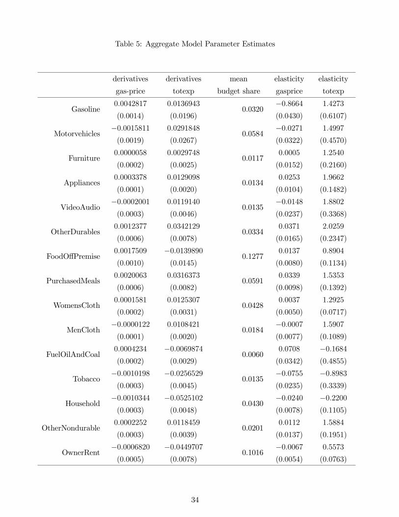
Table 5: Aggregate Model Parameter Estimates

derivatives

gas-price

derivatives

totexp

mean

budget share

elasticity

gasprice

elasticity

totexp

Gasoline0:0042817

(0:0014)

0:0136943

(0:0196)0.0320

�0:8664(0:0430)

1:4273

(0:6107)

Motorvehicles�0:0015811(0:0019)

0:0291848

(0:0267)0.0584

�0:0271(0:0322)

1:4997

(0:4570)

Furniture0:0000058

(0:0002)

0:0029748

(0:0025)0.0117

0:0005

(0:0152)

1:2540

(0:2160)

Appliances0:0003378

(0:0001)

0:0129098

(0:0020)0.0134

0:0253

(0:0104)

1:9662

(0:1482)

VideoAudio�0:0002001(0:0003)

0:0119140

(0:0046)0.0135

�0:0148(0:0237)

1:8802

(0:3368)

OtherDurables0:0012377

(0:0006)

0:0342129

(0:0078)0.0334

0:0371

(0:0165)

2:0259

(0:2347)

FoodO¤Premise0:0017509

(0:0010)

�0:0139890(0:0145)

0.12770:0137

(0:0080)

0:8904

(0:1134)

PurchasedMeals0:0020063

(0:0006)

0:0316373

(0:0082)0.0591

0:0339

(0:0098)

1:5353

(0:1392)

WomensCloth0:0001581

(0:0002)

0:0125307

(0:0031)0.0428

0:0037

(0:0050)

1:2925

(0:0717)

MenCloth�0:0000122(0:0001)

0:0108421

(0:0020)0.0184

�0:0007(0:0077)

1:5907

(0:1089)

FuelOilAndCoal0:0004234

(0:0002)

�0:0069874(0:0029)

0.00600:0708

(0:0342)

�0:1684(0:4855)

Tobacco�0:0010198(0:0003)

�0:0256529(0:0045)

0.0135�0:0755(0:0235)

�0:8983(0:3339)

Household�0:0010344(0:0003)

�0:0525102(0:0048)

0.0430�0:0240(0:0078)

�0:2200(0:1105)

OtherNondurable0:0002252

(0:0003)

0:0118459

(0:0039)0.0201

0:0112

(0:0137)

1:5884

(0:1951)

OwnerRent�0:0006820(0:0005)

�0:0449707(0:0078)

0.1016�0:0067(0:0054)

0:5573

(0:0763)

34

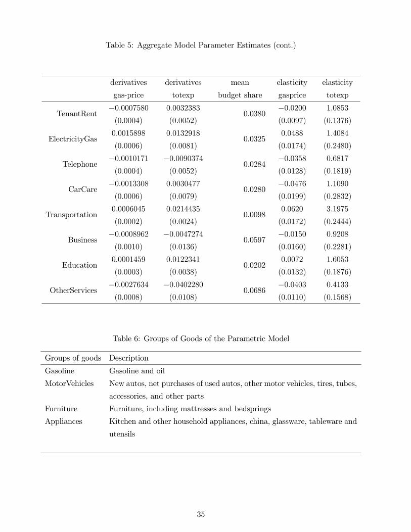
Table 5: Aggregate Model Parameter Estimates (cont.)

derivatives

gas-price

derivatives

totexp

mean

budget share

elasticity

gasprice

elasticity

totexp

TenantRent�0:0007580(0:0004)

0:0032383

(0:0052)0.0380

�0:0200(0:0097)

1:0853

(0:1376)

ElectricityGas0:0015898

(0:0006)

0:0132918

(0:0081)0.0325

0:0488

(0:0174)

1:4084

(0:2480)

Telephone�0:0010171(0:0004)

�0:0090374(0:0052)

0.0284�0:0358(0:0128)

0:6817

(0:1819)

CarCare�0:0013308(0:0006)

0:0030477

(0:0079)0.0280

�0:0476(0:0199)

1:1090

(0:2832)

Transportation0:0006045

(0:0002)

0:0214435

(0:0024)0.0098

0:0620

(0:0172)

3:1975

(0:2444)

Business�0:0008962(0:0010)

�0:0047274(0:0136)

0.0597�0:0150(0:0160)

0:9208

(0:2281)

Education0:0001459

(0:0003)

0:0122341

(0:0038)0.0202

0:0072

(0:0132)

1:6053

(0:1876)

OtherServices�0:0027634(0:0008)

�0:0402280(0:0108)

0.0686�0:0403(0:0110)

0:4133

(0:1568)

Table 6: Groups of Goods of the Parametric Model

Groups of goods Description

Gasoline Gasoline and oil

MotorVehicles New autos, net purchases of used autos, other motor vehicles, tires, tubes,

accessories, and other parts

Furniture Furniture, including mattresses and bedsprings

Appliances Kitchen and other household appliances, china, glassware, tableware and

utensils

35

Table 6: Groups of Goods of the Parametric Model (cont.)

Groups of goods Description

VideoAudio Video and audio goods, including musical instruments, and computer

goods

OtherDurable Ophthalmic products and orthopedic appliances, wheel goods, sports

and photographic equipment, boats, and pleasure aircraft, jewelry and

watches, books and maps, other durable house furnishings

FoodO¤Premise Food purchased for o¤-premise consumption

PurchasedMeals Purchased meals and beverages, food furnished to employees including

military and food produced and consumed on farms

Women�sCloth Women�s and children�s clothing and accessories, shoes

Men�sCloth Men�s and boys�clothing and accessories except shoes

FuelOilAndCoal Fuel oil and coal

Household Toilet articles and preparations, semidurable house furnishings, cleaning

and polishing preparations, and miscellaneous household supplies and

paper products, drug preparations and sundries

OtherNondurable Nondurable toys and sport supplies, stationery and writing supplies,

magazines, newspapers, and sheet music, �owers, seeds, and potted

plants

OwnerRent Owner-occupied nonfarm dwellings�space rent

TenantRent Tenant-occupied nonfarm dwellings�rent

ElectricityGas Electricity, gas, water and other sanitary services

Telephone Telephone and telegraph, domestic service, other household operation

CarCare Repair, greasing, washing, parking, storage, rental, and leasing, other

user-operated transportation

Transportation Purchased local transportation (mass transit systems, taxicab), pur-

chased intercity transportation (railway, bus, airline, other)

Education Higher education, nursery, elementary, and secondary schools, other

OtherServices Rental value of farm dwellings, other housing, Admissions to speci�ed

spectator amusements and other recreation, Religious and welfare activ-

ities, Foreign travel by U.S. residents

36

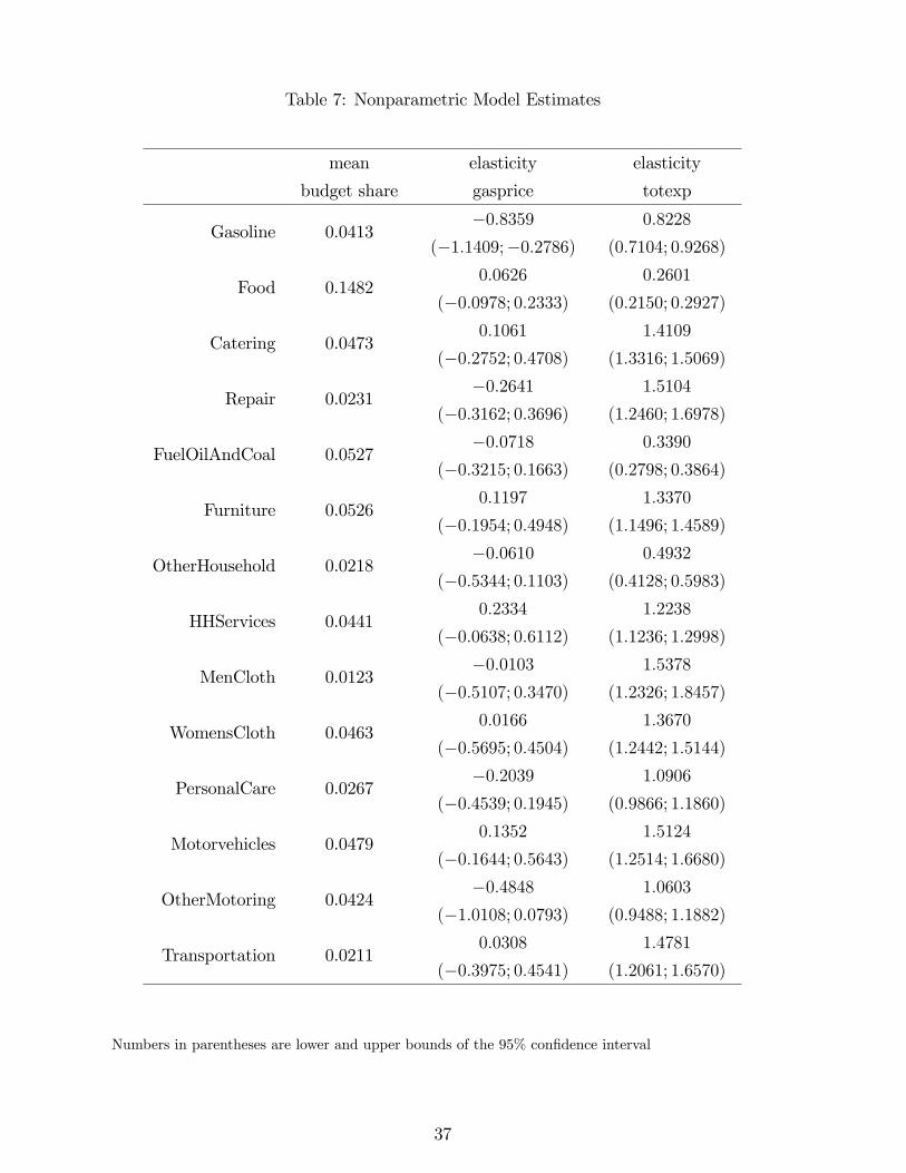
Table 7: Nonparametric Model Estimates

mean

budget share

elasticity

gasprice

elasticity

totexp

Gasoline 0.0413�0:8359

(�1:1409;�0:2786)0:8228

(0:7104; 0:9268)

Food 0.14820:0626

(�0:0978; 0:2333)0:2601

(0:2150; 0:2927)

Catering 0.04730:1061

(�0:2752; 0:4708)1:4109

(1:3316; 1:5069)

Repair 0.0231�0:2641

(�0:3162; 0:3696)1:5104

(1:2460; 1:6978)

FuelOilAndCoal 0.0527�0:0718

(�0:3215; 0:1663)0:3390

(0:2798; 0:3864)

Furniture 0.05260:1197

(�0:1954; 0:4948)1:3370

(1:1496; 1:4589)

OtherHousehold 0.0218�0:0610

(�0:5344; 0:1103)0:4932

(0:4128; 0:5983)

HHServices 0.04410:2334

(�0:0638; 0:6112)1:2238

(1:1236; 1:2998)

MenCloth 0.0123�0:0103

(�0:5107; 0:3470)1:5378

(1:2326; 1:8457)

WomensCloth 0.04630:0166

(�0:5695; 0:4504)1:3670

(1:2442; 1:5144)

PersonalCare 0.0267�0:2039

(�0:4539; 0:1945)1:0906

(0:9866; 1:1860)

Motorvehicles 0.04790:1352

(�0:1644; 0:5643)1:5124

(1:2514; 1:6680)

OtherMotoring 0.0424�0:4848

(�1:0108; 0:0793)1:0603

(0:9488; 1:1882)

Transportation 0.02110:0308

(�0:3975; 0:4541)1:4781

(1:2061; 1:6570)

Numbers in parentheses are lower and upper bounds of the 95% con�dence interval

37

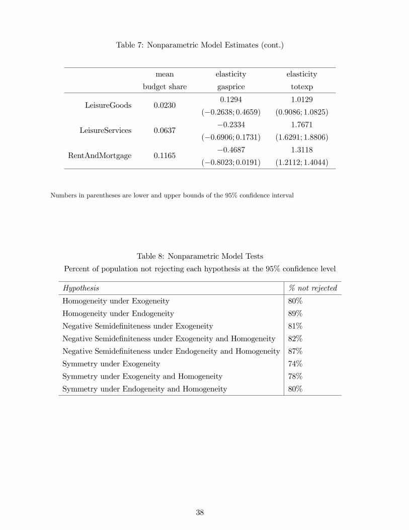
Table 7: Nonparametric Model Estimates (cont.)

mean

budget share

elasticity

gasprice

elasticity

totexp

LeisureGoods 0.02300:1294

(�0:2638; 0:4659)1:0129

(0:9086; 1:0825)

LeisureServices 0.0637�0:2334

(�0:6906; 0:1731)1:7671

(1:6291; 1:8806)

RentAndMortgage 0.1165�0:4687

(�0:8023; 0:0191)1:3118

(1:2112; 1:4044)

Numbers in parentheses are lower and upper bounds of the 95% con�dence interval

Table 8: Nonparametric Model Tests

Percent of population not rejecting each hypothesis at the 95% con�dence level

Hypothesis % not rejected

Homogeneity under Exogeneity 80%

Homogeneity under Endogeneity 89%

Negative Semide�niteness under Exogeneity 81%

Negative Semide�niteness under Exogeneity and Homogeneity 82%

Negative Semide�niteness under Endogeneity and Homogeneity 87%

Symmetry under Exogeneity 74%

Symmetry under Exogeneity and Homogeneity 78%

Symmetry under Endogeneity and Homogeneity 80%

38

Table 9: Groups of Goods of the Nonparametric Model

Groups of goods Description

Gasoline Gasoline and oil

Food Bread, meat and �sh, milk products, drinks, fruits and vegetables, other

food

Catering Restaurant meals, canteen meals, take-away meals and snacks

Repair Payments to contractors, including those for house painting and decorat-

ing, purchase of materials and tools (other than electrical tools)

FuelOilAndCoal Fuel oil and coal

Furniture New and second-hand furniture, �oor coverings, household textiles, mat-

tresses, pillows, cushions etc., electrical appliances (excluding audio-

visual equipment) and other household equipment

OtherHousehold Soap and detergents, other cleaning materials, toilet paper and other

HouseholdServices Postage, telephones charges, telephones, telemessages, domestic services,

fees and subscriptions

Men�sCloth Men�s clothing, including shirts and sportswear

Women�sCloth Women�s clothing, children�s clothing, other clothing and footwear

PersonalCare Personal articles, chemists goods, personal services

MotorVehicles Net purchases of new and second-hand cars, vans, motor cycles, scooters

OtherMotoring Repair and servicing of motor vehicles, spares and accessories, vehicle

tax and insurance

Transportation Rail fares, bus fares, taxi fares, car hire charges and other travel costs

LeisureGoods Records, toys, photo and sports goods, personal articles, books and news-

papers, gardening products

LeisureServices TV licences and rentals, entertainment and recreation, foreign holidays

and UK holidays

RentAndMortgage Rent, excluding rates and other charges paid together with rent, interest

payments on a representative mortgage

39