Regression Shrinkage and Selection via the Lasso

Robert Tibshirani

Journal of the Royal Statistical Society. Series B (Methodological), Vol. 58, No. 1. (1996), pp.267-288.

Stable URL:

http://links.jstor.org/sici?sici=0035-9246%281996%2958%3A1%3C267%3ARSASVT%3E2.0.CO%3B2-G

Journal of the Royal Statistical Society. Series B (Methodological) is currently published by Royal Statistical Society.

Your use of the JSTOR archive indicates your acceptance of JSTOR's Terms and Conditions of Use, available athttp://www.jstor.org/about/terms.html. JSTOR's Terms and Conditions of Use provides, in part, that unless you have obtainedprior permission, you may not download an entire issue of a journal or multiple copies of articles, and you may use content inthe JSTOR archive only for your personal, non-commercial use.

Please contact the publisher regarding any further use of this work. Publisher contact information may be obtained athttp://www.jstor.org/journals/rss.html.

Each copy of any part of a JSTOR transmission must contain the same copyright notice that appears on the screen or printedpage of such transmission.

JSTOR is an independent not-for-profit organization dedicated to and preserving a digital archive of scholarly journals. Formore information regarding JSTOR, please contact support@jstor.org.

http://www.jstor.orgMon Jun 4 21:31:15 2007

J. R. Statist. Soc. B (1996) 58, NO. 1,pp. 267-288

Regression Shrinkage and Selection via the Lasso

By ROBERT TIBSHIRANIt

University of Toronto, Canada

[Received January 1994. Revised January 19951

SUMMARY We propose a new method for estimation in linear models. The 'lasso' minimizes the residual sum of squares subject to the sum of the absolute value of the coefficients being less than a constant. Because of the nature of this constraint it tends to produce some coefficients that are exactly 0 and hence gives interpretable models. Our simulation studies suggest that the lasso enjoys some of the favourable properties of both subset selection and ridge regression. It produces interpretable models like subset selection and exhibits the stability of ridge regression. There is also an interesting relationship with recent work in adaptive function estimation by Donoho and Johnstone. The lasso idea is quite general and can be applied in a variety of statistical models: extensions to generalized regression models and tree-based models are briefly described.

Keywords: QUADRATIC PROGRAMMING; REGRESSION, SHRINKAGE; SUBSET SELECTION

1. INTRODUCTION

Consider the usual regression situation: we have data (xi, yi), i = 1, 2, . . ., N, where xi = (xi,, . . ., xi,)= and yi are the regressors and response for the ith observation. The ordinary least squares (OLS) estimates are obtained by minimizing the residual squared error. There are two reasons why the data analyst is often not satisfied with the OLS estimates. The first is prediction accuracy: the OLS estimates often have low bias but large variance; prediction accuracy can sometimes be improved by shrinking or setting to 0 some coefficients. By doing so we sacrifice a little bias to reduce the variance of the predicted values and hence may improve the overall prediction accuracy. The second reason is interpretation. With a large number of predictors, we often would like to determine a smaller subset that exhibits the strongest effects.

The two standard techniques for improving the OLS estimates, subset selection and ridge regression, both have drawbacks. Subset selection provides interpretable models but can be extremely variable because it is a discrete process- regressors are either retained or dropped from the model. Small changes in the data can result in very different models being selected and this can reduce its prediction accuracy. Ridge regression is a continuous process that shrinks coefficients and hence is more stable: however, it does not set any coefficients to 0 and hence does not give an easily interpretable model.

We propose a new technique, called the lasso, for 'least absolute shrinkage and selection operator'. It shrinks some coefficients and sets others to 0, and hence tries to retain the good features of both subset selection and ridge regression.

tAddress for correspondence: Department of Preventive Medicine and Biostatistics, and Department of Statistics, University of Toronto, 12 Queen's Park Crescent West, Toronto, Ontario, M5S 1A8, Canada. E-mail: tibs@utstat.toronto.edu

O 1996 Royal Statistical Society 003!5-9246196158267

268 TIBSHIRANI [No. 1,

In Section 2 we define the lasso and look at some special cases. A real data example is given in Section 3, while in Section 4 we discuss methods for estimation of prediction error and the lasso shrinkage parameter. A Bayes model for the lasso is briefly mentioned in Section 5. We describe the lasso algorithm in Section 6. Simulation studies are described in Section 7. Sections 8 and 9 discuss extensions to generalized regression models and other problems. Some results on soft thresholding and their relationship to the lasso are discussed in Section 10, while Section 11 contains a summary and some discussion.

2. THE LASSO

2.1. DeJinition Suppose that we have data (xi, yi), i = 1, 2, . . ., N, where xi = (xi,, . . ., x ~ ~ ) ~are

the predictor variables and yi are the responses. As in the usual regression set-up, we assume either that the observations are independent or that the yis are conditionally independent given the xi$. We assume that the xii are standardized so that Xixii/N = 0,- &x;/'N-= !.

Letting p = (pl, . . ., the lasso estimate (8, b) is defined by

N

= arg "n -a - pjXij)2/ subject to 1.1 ( t. (I) i

Here t >, 0 is a tuning parameter. Now, for all t, the solution for a is 8 = j . We can assume without loss of generality that j = 0 and hence omit a.

Computation of the solution to equation (1) is a quadratic programming problem with linear inequality constraints. We describe some efficient and stable algorithms for this problem in Section 6.

The parametgr t 2 0 controls the amount of shrinkage that is applied to the estimates. Let be the full least squares estimates and let to = XI#?:[. Values of t < to will cause shrinkage of the solutions towards 0, and some coefficients may be exactly equal to 0. For example, if t = to/2, the effect will be roughly similar to finding the best subset of sizep/2. Note also that the design matrix need not be of full rank. In Section 4 we give some data-based methods for estimation of t.

The motivation for the lasso came from an interesting proposal of Breiman (1993). Breiman's non-negative garotte minimizes

Nc (Yi -a-x subject to cj >, 0, x c , < t. (2) i= 1 i

The garotte starts with the OLS estimates and shrinks them by non-negative factors whose sum is constrained. In extensive simulation studies, Breiman showed that the garotte has consistently lower prediction error than subset selection and is competitive with ridge regression except when the true model has many small non- zero coefficients.

A drawback of the garotte is that its solution depends on both the sign and the magnitude of the OLS estimates. In overfit or highly correlated settings where the OLS estimates behave poorly, the garotte may suffer as a result. In contrast, the lasso avoids the explicit use of the OLS estimates.

19961 REGRESSION SHRINKAGE AND SELECTION 269

Frank and Friedman (1993) proposed using a bound on the Lq-norm of the parameters, where q is some number greater than or equal to 0; the lasso corresponds to q = 1. We discuss this briefly in Section 10.

2.2. Orthonormal Design Case Insight about the nature of the shrinkage can be gleaned from the orthonormal

design case. Let X be the n x p design matrix with ijth entry xij, and suppose that XTX = I, the identity matrix.

The solutions to equation (1) are easily shown to be

where y is determined by the condition x1jjl = t. Interestingly, this has exactly the same form as the soft shrinkage proposals of Donoho and Johnstone (1994) and Donoho et al. (1995), applied to wavelet coefficients in the context of function estimation. The connection between soft shrinkage and a minimum L1-norm penalty was also pointed out by Donoho et al. (1992) for non-negative parameters in the context of signal or image recovery. We elaborate more on this connection in Section 10.

In the orthonormal design case, best subset selection of size k reduces to choosing the k largest coefficients in absolute ~(alue~and s%tting the rest to 0. For some choice of h this is equivalent to setting /3, =& if J&J> h and to 0 otherwise. Ridge regression minimizes

or, equivalently, minimizes

The ridge solutions are

where y depends on h or t. The garotte estimates are

Fig. 1 shows the form of these functions. Ridge regression scales the coefficients by a constant factor, whereas the lasso translates by a constant factor, truncating at 0. The garotte function is very similar to the lasso, with less shrinkage for larger coefficients. As our simulations will show, the differences between the lasso and garotte can be large when the design is not orthogonal.

270 TIBSHIRANI Fro. 1,

2.3. Geometry of Lasso It is clear from Fig. 1 why the lasso will often produce coefficients that are exactly

0. Why does this happen in the general (non-orthogonal) setting? And why does it not occur with ridge regression, which uses the constraint ):,!I; < t rather than XI,!I,l < t? Fig. 2 provides some insight for the case p = 2.

The criterion EN,,(yi - Xj equals the quadratic function

(P- p ) T ~ T ~ ( p -p )

(plus a constant). The elliptical contours of this function are shown by the full curves in Fig. 2(a); they are centred at the OLS estimates; the constraint region is the rotated square. The lasso solution is the first place that the contours touch the square, and this will sometimes occur at a corner, corresponding to a zero coefficient. The picture for ridge regression is shown in Fig. 2(b): there are no corners for the contours to hit and hence zero solutions will rarely result.

An interesting question emerges from this picture: can tbe signs of the lasso estimates be different from those of the least squares estimates &?Since the variables are standardized, when p = 2 the principal axes of the contours are at +45" to the co-ordinate axes, and we can :how that the contours must contact the square in the same quadrant that contains p.However, whenp > 2 and there is at least moderate correlation in the data, this need not be true. Fig. 3 shows an example in three dimensions. The view in Fig. 3(b) confirms that the ellipse touches the constraint region in an octant different from the octant in which its centre lies.

beta beta

(a) (b)

beta beta

(c) (dl

Fig. 1. (a) Subset regression, (b) ridge regression, (c) the lasso and (d) the garotte: -, form of coefficient shrinkage in the orthonormal design case; ..--.......,45"-line for reference

REGRESSION SHRINKAGE AND SELECTION 271

(a) (b)

Fig. 2. Estimation picture for (a) the lasso and (b) ridge regression

Fig. 3. (a) Example in which the lasso estimate falls in an octant different from the overall least squares estimate; (b) overhead view

Whereas the garotte retains the sign of each &,the lasso can change signs. Even in cases where the lasso estimate has the same sign vector as the garotte, the preseGce of the OLS estimates in the garotte can make it behave differently. The moiel X cjp0xiiwith con- straint X cj 5 t can be written as X Bjxu with constraint X 8/14< t . 1f for example p = 2 and 8; > & > 0 then the effect would be to stretch the square in Fig. 2(a) horizontally. As a result, larger values of and smaller values of /Iz will be favoured by the garotte.

2.4. More on Two-predictor Case Suppose- that p =2, and assume without loss of generality that the least squares

estimates 6 are both positive. Then we can show that the lasso estimates are

TIBSHIRANI

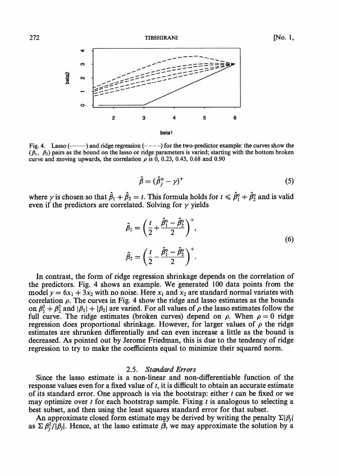
Fig. 4. Lasso (-1 and ridge regression (- ---) for the two-predictor example: the curves show the (PI , p2) pairs as the bound on the lasso or ridge parameters is varied; starting with the bottom broken curve and moving upwards, the correlation p is 0, 0.23, 0.45, 0.68 and 0.90

where y is chosen so that PI + ,62 = t. This formula holds for t < & + B," and is valid even if the predictors are correlated. Solving for y yields

In contrast, the form of ridge regression shrinkage depends on the correlation of the predictors. Fig. 4 shows an example. We generated 100 data points from the model y = 6x1+ 3x2 with no noise. Here x l and x2 are standard normal variates with correlation p. The curves in Fig. 4 show the ridge and lasso estimates as the bounds on /3: + /3; and IS11 + 1p21are varied. For all values of p the lasso estimates follow the full curve. The ridge estimates (broken curves) depend on p. When p = 0 ridge regression does proportional shrinkage. However, for larger values of p the ridge estimates are shrunken differentially and can even increase a little as the bound is decreased. As pointed out by Jerome Friedman, this is due to the tendency of ridge regression to try to make the coefficients equal to minimize their squared norm.

2.5. Standard Errors Since the lasso estimate is a non-linear and non-differentiable function of the

response values even for a fixed value oft, it is difficult to obtain an accurate estimate of its standard error. One approach is via the bootstrap: either t can be fixed or we may optimize over t for each bootstrap sample. Fixing t is analogous to selecting a best subset, and then using the least squares standard error for that subset.

An approximate closed form estimate may be derived by writing the penalty CI/3jl as C /3;/I/3jI. Hence, at the lasso estimate P, we may approximate the solution by a

19961 REGRESSION SHRINKAGE AND SELECTION 273

ridge regression of the fo-m P* = (XTX+AW-)-'XTy where W is a diagonal matrix with diagonal elements Ipjl, W- denotes the generalized inverse of W and h is chosen so that ZJBjl*= t . The covariance matrix of the estimates may then be approximated by

where G2 is an estimate of the error variance. A difficylty with this formula is that it gives an estimated variance of 0 for predictors with = 0.

This approximation also suggests an iterated ridge regression algorithm for computing the lasso estimate itself, but this turns out to be quite inefficient. However, it is useful for selection of the lasso parameter t (Section 4).

3. EXAMPLE -PROSTATE CANCER DATA

The prostate cancer data come from a study by Stamey et al. (1989) that examined the correlation between the level of prostate specific antigen and a number of clinical measures, in men who were about to receive a radical prostatectomy. The factors were log(cancer volume) (lcavol), logbrostate weight) (lweight), age, log(benign prostatic hyperplasia amount) (lbph), seminal vesicle invasion (svi), log(capsu1ar penetration) (lcp), Gleason score (gleason) and percentage Gleason scores 4 or 5 (pgg45). We fit a linear model to logbrostate specific antigen) (lpsa) after first standardizing the predictors.

Fig. 5. Lasso shrinkage of coefficients in the prostate cancer example: each curve represents a coefficient (labelled on the right) as a function of the (scaled) lasso parameter s = t/CI$I (the intercept is not plotted); the broken line represents the model for s =0.44, selected by generalized cross-validation

274 TIBSHIRANI [No. 1,

Fig. 5 shows the lasso estimates as a function of standardized bound s = t / ~ l p ~ .Notice that the absolute value of each coefficient tends to 0 as s goes to 0. In t$is example, the curves decrease in a monotone fashion to 0, but this does not always happen in general. This lack of monotonicity is shared by ridge regression and subset regression, where for example the best subset of size 5 may not contain the best subset of size 4. The vertical broken line represents the model for s = 0.44, the optimal value selected by generalized cross-validation. Roughly, this corresponds to keeping just under half of the predictors.

Table 1 shows the results for the full least squares, best subset and lasso procedures. Section 7.1 gives the details of the best subset procedure that was used. The lasso gave non-zero coefficients to lcavol, lweight and svi; subset selection chose the same three predictors. Notice that the coefficients and 2-scores for the selected predictors from subset selection tend to be larger than the full model values: this is common with positively correlated predictors. However, the lasso shows the opposite effect, as it shrinks the coefficients and 2-scores from their full model values.

The standard errors in the penultimate column were estimated by bootstrap resampling of residuals from the full least squares fit. The standard errors were computed by fixing s at its optimal value 0.44 for the original data set. Table 2

TABLE 1 Results for the prostate cancer example

Predictor Least squares results Subset selection results Lasso results

Coefficient Standard Z-score Coefficient Standard Z-score Coefficient Standard Z-score error error error

1 intcpt 2 lcavol 3 lweight 4 age 5 lbph 6 svi 7 1cp 8 gleason 9 pgg45

TABLE 2 Standard error estimates for the prostate cancer example

Predictor Coefficient Bootstrap standard error Standard error approximation (7)

Fixed t Varying t

1 intcpt 2 lcavol 3 lweight 4 age 5 lbph 6 svi 7 1cp8 gleason 9 pgg45

REGRESSION SHRINKAGE A m SELECTION

lcavol lweight age lbph svi Icp gleasan pgg45

Fig. 6. Box plots of 200 bootstrap values of the lasso coefficient estimates for the eight predictors in the prostate cancer example

compares the ridge approximation formula (7) with the fixed t bootstrap, and the bootstrap in which t was re-estimated for each sample. The ridge formula gives a fairly good approximation to the fixed t bootstrap, except for the zero coefficients. Allowing t to vary incorporates an additional source of variation and hence gives larger standard error estimates. Fig. 6 shows box plots of 200 bootstrap replications of the lasso estimates, with s fixed at the estimated value 0.44. The predictors whose estimated coefficient is 0 exhibit skewed bootstrap distributions. The central 90% percentile intervals (fifth and 95th percentiles of the bootstrap distributions) all contained the value 0, with the exceptions of those for lcavol and svi.

4. PREDICTION ERROR AND ESTIMATION OF t

In this section we describe three methods for the estimation of the lasso parameter t : cross-validation, generalized cross-validation and an analytical unbiased estimate of risk. Strictly speaking the first two methods are applicable in the 'X-random' case, where it is assumed that the observations (X, Y) are drawn from some unknown distribution, and the third method applies to the X-fixed case. However, in real problems there is often no clear distinction between the two scenarios and we might simply choose the most convenient method.

Suppose that

where E(E) = 0 and var(6) = a2.The mean-squared error of an estimate ij(X) is defined by

the expected value taken over the joint distribution of X and Y, with 6 6 ) fixed. A similar measure is the prediction error of ij(X) given by

We estimate the prediction error for the lasso procedure by fivefold cross-validation as described (for example) in chapter 17 of Efron and Tibshi~ani (1993). The lasso is indexed in terms of the normalized parameter s = t / C /IT, and the prediction error is estimated over a grid of values of s from 0 to 1 inclusive. The value s yielding the lowest estimated PE is selected.

276 TIBSHIRANI [No. 1 ,

Simulation resqlts are reported in terms of ME rather than PE. For the linear models q(X) = XP considered in this paper, the mean-squared error has the simple form

where V is the population covariance matrix of X. A second method for estimating t may be derived from a linear approximation to

the lasso estimate. We write the constraint CIpjl < t as C #/Ipjl < t. This constraint is equivalent to adding a Lagrangian penalty h C $/1pjl to the residual _sum of squares, with h depending on t. Thus we may write the constrained solution P as the ridge regression estimator

where W = diag(ljjl) and W- denotes a gensralized inverse. Therefore the number of effective parameters in the constrained fit p may be approximated by

Letting rss(t) be the residual sum of squares for the constrained fit with constraint t, we construct the generalized cross-validation style statistic

Finally, we outline a third method based on Stein's unbiased estimate of risk. Suppose that z is a multivariate normal random vector with mean p and variance the identity matrix. Let ji be an estimator of p , and write ,G =z +g(z) where g is an almost differential function from RP to RP (see definition 1 of Stein (1981)). Then Stein (1981) showed that

We may gpply this result to the lasso estimator (3). Denote the es t i~ated standard error of 89 by ? = 3/JN, where G2 = C (vi - f J 2 / ( ~-p). Then the BY/? are (condi- tionally on X) approximately independent standard normal variates, and from equation (1 1) we may derive the formula

as an approxjmately unbiased estimate of the risk or mean-square error ~ { f i ( ~ ) -P)', where B,(y) = sign(p;)(lfl/PI - y)'. Donoho and Johnstone (1994) gave a similar formula in the function gstimation setting. Hence an estimate of y can be obtained as the minimizer of R{P(y)):

19961 REGRESSION SHRINKAGE AND SELECTION

From this we obtain an estimate of the lasso parameter t:

Although the derivation of t^ assumes an orthogonal design, we may still try to use it in the usual non-orthogonal setting. Since the predictors have been standardized, the optimal value of t is roughly a function of the overall signal-to-noise ratio in the data, and it should be relatively insensitive to the covariance of X. (In contrast, the form of the lasso estimator is sensitive to the covariance and we need to account for it properly.)

The simulated examples in Section 7.2 suggest that this method gives a useful estimate of t. But we can offer only a heuristic argument in favour of it. Suppose that XTX =V and let Z =XV-'/~,8 = pv-'l2. Since the columns of X are standardized, the region C)Ojl < t differs from the region Clfijl < t in shape but has roughly the same-sized marginal projections. Therefore the optimal value of ;should be about the same in each instance.

Finally, note that the Stein method enjoys a significant computational advantage over the cross-validation-based estimate oft. In our experiments we optimized over a grid of 15 values of the lasso parameter t and used fivefold cross-validation. As a result, the cross-validation approach required 75 applications of the model optim- ization procedure of Section 6 whereas the Stein method required only one. The requirements of the generalized cross-validation approach are intermediate between the two, requiring one application of the optimization procedure per grid point.

5. LASSO AS BAYES ESTIMATE

The lasso constraint CISjl < t is equivalent to the addition of a penalty term h CISjl to the residual sum of squares (see Murray et al. (1981), chapter 5). Now lSjl is proportional to the (minus) log-density of the double-exponential distribution. As a result we can derive the lasso estimate as the Bayes posterior mode under inde- pendent double-exponential priors for the Pis,

1 l SjlAB~)=Z;ex(- 7)

with t= l lh. Fig. 7 shows the double-exponential density (full curve) and the normal density

(broken curve); the latter is the implicit prior used by ridge regression. Notice how the double-exponential density puts more mass near 0 and in the tails. This reflects the greater tendency of the lasso to produce estimates that are either large or 0.

6. ALGORITHMS FOR FINDING LASSO SOLUTIONS

We fix t 2 0. Problem (1) can be expressed as a least squares problem with 2p inequality constraints, corresponding to the 2p different possible signs for the Pis.

TIBSHIRANI

(-) Double-exponential density

beta

Fig. 7. and normal density (- - - - -): the former is the implicit prior used by the lasso; the latter by ridge regression

Lawson and Hansen (1974) provided the ingredients for a procedure which solves the linear least squares problem subject to a general linear inequality constraint GP < h. Here G is an m x p matrix, corresponding to m linear inequality constraints on the p- vector p. For our problem, however, m = 2P may be very large so that direct application of this procedure is not practical. However, the problem can be solved by introducing the inequality constraints sequentially, seeking a feasible solution satisfying the so-called Kuhn-Tucker conditions (Lawson and Hansen, 1974). We outline the procedure below.

Let g(P) = I=:,- and let 4 , i = 1, 2, . . ., 2P be the p-tuples of the ( y i c , ~ ~ x ~ ) ~ , form ( k l , f1, . . ., f I). Then the condition Zlp,l < t is equivalent to STP < t for all i. For a given ,By let E = {i: 6Tp = t) and S= {i: 6Tp < t). The set E is the equality set, corresponding to those constraints which are exactly met, whereas S is the slack set, corresponding to those constraints for which equality does not hold. Denote by GEthe matrix whose rows are bi for i E E. Let 1 be a vector of 1s of length equal to the number of rows of GE.

The following algorithm starts with E = {io) where 6, = sign@), b being the overall least squares estimate. It solves the least squares problem subject to 6:P < t and then checks whether ZIpjl< t. If so, the computation is complete; if not, the violated constraint is added to E and the process is continued until Zlpjl< t.

Here is an outline of the algorithm.

(a) Start with E = {io) where 6, = sign@), @' being the overall least squares estimaie.

(b) Find P to-minimize g(P) subject to GEP < tl. (c) While {Zlpjl> t), (d) add i to the set E where bi = sign@). Find f i to minimize g(P) subject to

GEP < tl. This procedure must always converge in a finite number of steps since one element

is added to the set E a t each step, and there is a total of 2p elements. The final iterate

REGRESSION SHRINKAGE AND SELECTION

TABLE 3 Results for example I t

Method Median mean-squared Average no. of Average i error 0 coefficients

Least squares 2.79 (0.12) 0.0 -Lasso (cross-validation) 2.43 (0.14) 3.3 0.63 (0.01) Lasso (Stein) 2.07 (0.10) 2.6 0.69 (0.02) Lasso (generalized cross-validation) 1.93 (0.09) 2.4 0.73 (0.01) Garotte 2.29 (0.16) 3.9 -Best subset selection 2.44 (0.16) 4.8 -

Ridge regression 3.21 (0.12) 0.0 -

?Standard errors are given in parentheses.

is a solution to the original problem since the Kuhn-Tucker conditions are satisfied for the sets E and S at convergence.

A modification of this procedure removes elements from E in step (d) for which the equality constraint is not satisfied. This is more efficient but it is not clear how to establish its convergence.

The fact that the algorithm must stop after at most 2p iterations is of little comfort if p is large. In practice we have found that the average number of iterations required is in the range (0.5p, 0.75~) and is therefore quite acceptable for practical purposes.

A completely different algorithm for this problem was suggested by David Gay. We write each ,!Ij as pi+-PI:, where p,? and PI: are non-negative. Then we solve the least squares problem with the constraints 2 0, /I,: 2 0 and C pi++ Cj PI: < t . In this way we transform the original problem (p variables, 2p constraints) to a new problem with more variables (2p) but fewer constraints (2p + I). One can show that this new problem has the same solution as the original problem.

Standard quadratic programming techniques can be applied, with the convergence assured in 2p + 1 steps. We have not extensively compared these two algorithms but in examples have found that the second algorithm is usually (but not always) a little faster than the first.

7. SIMULATIONS

7.1. Outline In the following examples, we compare the full least squares estimates with the

lasso, the non-negative garotte, best subset selection and ridge regression. We used fivefold cross-validation to estimate the regularization parameter in each case. For best subset selection, we used the 'leaps' procedure in the S language, with fivefold cross-validation to estimate the best subset size. This procedure is described and studied in Breiman and Spector (1992) who recommended fivefold or tenfold cross- validation for use in practice.

For completeness, here are the details of the cross-validation procedure. The best subsets of each size are first found for the original data set: call these So, S1, . . ., Sp. (So represents the null nodel; since j = 0 the fitted values are 0 for this model.) Denote the full training set by T, and the cross-validation training and test sets by T - Tv and Tv, for v = 1, 2, . . ., 5. For each cross-validation fold v, we find the best

TIBSHIRANI

TABLE 4 Most frequent models selected by the lasso (generalized cross-validation) in example I

Model Proportion

1245678 0.055 123456 0.050 1258 0.045 1245 0.045 13 others 125 (and 5 others) 0.025

subsets of each size for the data T - Tv: call these S;;, S';, . . ., 5.Let PEv(J) be the prediction error when St;is applied to the test data Tv, and form the estimate

We find the j that minimizes PE(J) and our selected model is Sj.This is not the same as estimating the prediction error of the fixed models So,Sly. . ., S, and then choosing the one with the smallest prediction error. This latter procedure is described in Zhang (1993) and Shao (1992), and can lead to inconsistent model selection unless the cross-validation test set TV grows at an appropriate asymptotic rate.

7.2. Example 1 In this example we simulated 50 data sets consisting of 20 observations from the

model

where p = (3, 1.5, 0, 0, 2, 0, 0, O)T and E is standard normal. The correlation between xiand xj was pii-jl with p = 0.5. We set a = 3, and this gave a signal-to-noise ratio of approximately 5.7. Table 3 shows the mean-squared errors over 200 simulations from this model. The lasso performs the best, followed by the garotte and ridge regression.

Estimation of the lasso parameter by generalized cross-validation seems to per- form best, a trend that we find is consistent through all our examples. Subset

TABLE 5 Most frequent models selected by all-subsets

regression in example I

Model Proportion

0.240 0.200 0.095

1257 0.040

--- --- -- --- -

--- --

REGRESSION SHRINKAGE AND SELECTION

o l n n I full Is lasso garotte best subset ridge

P

..............+......"'........+ ...... 8--- ........ --- r-- r--...... ...............

0

full Is lasso garotte best subset ridge

01 ---+ - - ........ . . . ... ..............

U + *. ;+---L--' Y , o n

full Is lasso garotte best subset ridge

Y J n full Is

C ) .

7

7 ,

...............

n

full Is

---

0

lasso

.......

lasso

---

0

garotte

garotte

-0

best subset

.......

best subset

---

n ridge

---L--n

ridge

..............

full Is l a w garotte best subset ridge

01

?'

U

r--

---L--full Is

---

lasso garotte

........

0

1

best subset

U

---b--ridge

cu 7

0

9 ' .

............... .......

---L-, 8

full Is

--- --

lasso

........

a garotte

n

best subset B

ridse

Fig. 8. Estimates for the eight coefficients in example 1,excluding the intercept: ..........,true coefficients

TIBSHIRANI

TABLE 6 Results for example 2-f

Method Median mean-squared Average no. of Average .? error 0 coefficients

-Least squares 6.50 (0.64) 0.0 Lasso (cross-validation) 5.30 (0.45) 3.0 0.50 (0.03) Lasso (Stein) 5.85 (0.36) 2.7 0.55 (0.03) Lasso (generalized cross-validation) 4.87 (0.35) 2.3 0.69 (0.23) Garotte 7.40 (0.48) 4.3 -

Subset selection 9.05 (0.78) 5.2 -Ridge regression 2.30 (0.22) 0.0 -

?Standard errors are given in parentheses.

selection picks approximately the correct number of zero coefficients (5), but suffers from too much variability as shown in the box plots of Fig. 8.

Table 4 shows the five most frequent models (non-zero coefficients) selected by the lasso (with generalized cross-validation): although the correct model (1, 2, 5) was chosen only 2.5% of the time, the selected model contained (1, 2, 5) 95.5% of the time. The most frequent models selected by subset regression are shown in Table 5. The correct model is chosen more often (24% of the time), but subset selection can also underfit: the selected model contained (1, 2, 5) only 53.5% of the time.

7.3. Example 2 The second example is the same as example 1, but with Bj = 0.85, V j and a = 3; the

signal-to-noise ratio was approximately 1.8. The results in Table 6 show that ridge regression does the best by a good margin, with the lasso being the only other method to outperform the full least squares estimate.

7.4. Example 3 For example 3 we chose a set-up that should be well suited for subset selection.

The model is the same as example 1, but with ,B =(5, 0, 0, 0, 0, 0, 0, 0) and a = 2 so that the signal-to-noise ratio was about 7.

The results in Table 7 show that the garotte and subset selection perform the best,

TABLE 7 Results for example 3-f

Method Median mean-squared Average no. of Average j. error 0 coefficients

Least squares 2.89 (0.04) 0.0 -Lasso (cross-validation) 0.89 (0.01) 3.0 0.50 (0.03) Lasso (Stein) 1.26 (0.02) 2.6 0.70 (0.01) Lasso (generalized cross-validation) 1.02 (0.02) 3.9 0.63 (0.04) Garotte 0.52 (0.01) 5.5 -Subset selection 0.64 (0.02) 6.3 -Ridge regression 3.53 (0.05) 0.0 -

?Standard errors are given in parentheses.

REGRESSION SHRINKAGE AND SELECTION

TABLE 8 Results for example 4-f

Method Median mean-squared Average no. of Average .? error 0 coefficients

Least squares 137.3 (7.3) 0.0 -Lasso (Stein) 80.2 (4.9) 14.4 0.55 (0.02) Lasso (generalized cross-validation) 64.9 (2.3) 13.6 0.60 (0.88) Garotte 94.8 (3.2) 22.9 -

Ridge regression 57.4 (1.4) 0.0 -

?Standard errors are given in parentheses.

followed closely by the lasso. Ridge regression does poorly and has a higher mean- squared error than do the full least squares estimates.

7.5. Example 4 In this example we examine the performance of the lasso in a bigger model. We

simulated 50 data sets each having 100 observations and 40 variables (note that best subsets regression is generally considered impractical for p > 30). We defined predictors xii= zii+ ziwhere ziiand ziare independent standard normal variates. This induced a pairwise correlation of 0.5 among the predictors. The coefficient vector was p = (0, 0, . . ., 0, 2, 2, . . ., 2, 0, 0, . . ., 0, 2, 2, . . ., 2), there being 10 repeats in each block. Finally we defined y = PTx+ 156 where 6 was standard normal. This produced a signal-to-noise ratio of roughly 9. The results in Table 8 show that the ridge regression performs the best, with the lasso (generalized cross- validation) a close second.

The average value of the lasso coefficients in each of the four blocks of 10 were 0.50 (0.06), 0.92 (0.07), 1.56 (0.08) and 2.33 (0.09). Although the lasso only produced 14.4 zero coefficients on average, the average value of 3 (0.55) was close to the true proportion of 0s (0.5).

8. APPLICATION TO GENERALIZED REGRESSION MODELS

The lasso can be applied to many other models: for example Tibshirani (1994) described an application to the proportional hazards model. Here we briefly explore the application to generalized regression models.

Consider any model indexed by a vector parameter P, for which estimation is carried out by maximization of a function I@); this may be a log-likelihood function or some other measure of fit. To apply the lasso, we maximize l(P) under the constraint CIPjl < t . It might be possible to carry out this maximization by a general (non-quadratic) programming procedure. Instead, we consider here models for which a quadratic approximation to l v ) leads to an iteratively reweighted least squares (IRLS) procedure for computation of P. Such a procedure is equivalent to a Newton-Raphson algorithm. Using this approach, we can solve the constrained problem by iterative application of the lasso algorithm, within an IRLS loop. Convergence of this procedure is not ensured in general, but in our limited experience it has behaved quite well.

284 TIBSHIRANI [No. 1,

8.1. Logistic Regression For illustration we applied the lasso to the logistic regression model for binary

data. We used the kyphosis data, analysed in Hastie and Tibshirani (1990), chapter 10. The response is kyphosis (0 = absent, 1 =present); the predictors xl = age, x2 = number of vertebrae levels and x3 = starting vertebrae level. There are 83 obser- vations. Since the predictor effects are known to be non-linear, we included squared terms in the model after centring each of the variables. Finally, the columns of the data matrix were standardized.

The linear logistic fitted model is

Backward stepwise deletion, based on Akaike's information criterion, dropped the x$-term and produced the model

The lasso chose 3 = 0.33, giving the model

Convergence, defined as the 11fi"'"-b0'd112< was obtained in five iterations.

9. SOME FURTHER EXTENSIONS

We are currently exploring two quite different applications of the lasso idea. One application is to tree-based models, as reported in LeBlanc and Tibshirani (1994). Rather than prune a large tree as in the classification and regression tree approach of Breiman et al. (1984), we use the lasso idea to shrink it. This involves a constrained least squares operation much like that in this paper, with the parameters being the mean contrasts at each node. A further set of constraints is needed to ensure that the shrunken model is a tree. Results reported in LeBlanc and Tibshirani (1994) suggest that the shrinkage procedure gives more accurate trees than pruning, while still producing interpretable subtrees.

A different application is to the multivariate adaptive regression splines (MARS) proposal of Friedman (1991). The MARS approach is an adaptive procedure that builds a regression surface by sum of products of piecewise linear basis functions of the individual regressors. The MARS algorithm builds a model that typically includes basis functions representing main effects and interactions of high order. Give the adaptively chosen bases, the MARS fit is simply a linear regression onto these bases. A backward stepwise procedure is then applied to eliminate less important terms.

In on-going work with Trevor Hastie, we are developing a special lasso-type algorithm to grow and prune a MARS model dynamically. Hopefully this will produce more accurate MARS models which also are interpretable.

The lasso idea can also be applied to ill-posed problems, in which the predictor matrix is not full rank. Chen and Donoho (1994) reported some encouraging results for the use of lasso-style constraints in the context of function estimation via wavelets.

19961 REGRESSION SHRINKAGE AND SELECTION 285

10. RESULTS ON SOFT THRESHOLDING

Consider the special case of an orthonormal design XTX =I. Then the lasso estimate has the form

This is called a 'soft threshold' estimator by Donoho and Johnstone (1994); they applied this estimator to the coefficients of a wavelet transform of a function measured with noise. They then backtransformed to obtain a smooth estimate of the function. Donoho and Johnstone proved many optimality results for the soft threshold estimator and then translated these results into optimality results for function estimation.

Our interest here is not in function estimation but in the coefficients themselves. We give one of Donoho and Johnstone's results here. It shows that asymptotically the soft threshold estimator (lasso) comes as close as subset selection to the performance of an ideal subset selector- one that uses information about the actual parameters.

Suppose that

where ci -- N(0, a2) and the design matrix is orthonormal. Then we can write

where zj -- N(0, a2). We consider estimation of p under squared error loss, with risk

Consider the family of diagonal linear projections

This estimator either keeps or $ills a parameter 6,i.e. it does subset selection. Now we incur a risk of d if we use 6,and /37 if we use an estimate of 0 instead. Hence the ideal choice of Jj is I(I/3jl > a), i.e. we keep only those predictors whose true coefficient is larger than the noise level. Call the risk of this estimator RDP: of course this estimator cannot be constructed since the are unknown. Hence RDP is a lower bound on the risk that we can hope to attain.

Donoho andJohtstone (1994) proved that the hard threshold (subset selection) estimator Jj = &'1(1&'1 > y) has risk

p) < (2 logp + 1) (2+ RDP).~ d , (16)

Here y is chosen as a(2 log n)'I2, the choice giving smallest asymptotic risk. They also showed that the soft threshold estimator (13) with y = a(2 log n)'I2 achieves the same asymptotic rate.

286 TIBSHIRANI [No. 1 ,

These results lend some support to the potential utility of the lasso in linear models. However, the important differences between the various approaches tend to occur for correlated predictors, and theoretical results such as those given here seem to be more difficult to obtain in that case.

1 1 . DISCUSSION

In this paper we have proposed a new method (the lasso) for shrinkage and selection for regression and generalized regression problems. The lasso does not focus on subsets but rather defines a continuous shrinking operation that can produce coefficients that are exactly 0. We have presented some evidence in this paper that suggests that the lasso is a worthy competitor to subset selection and ridge regression. We examined the relative merits of the methods in three different scenarios:

(a) small number of large efects-subset selection does best here, the lasso not quite as well and ridge regression does quite poorly;

(b) small to moderate number of moderate-sized efects-the lasso does best, followed by ridge regression and then subset selection;

(c) large number of small efects-ridge regression does best by a good margin, followed by the lasso and then subset selection.

Breiman's garotte does a little better than the lasso in the first scenario, and a little worse in the second two scenarios. These results refer to prediction accuracy. Subset selection, the lasso and the garotte have the further advantage (compared with ridge regression) of producing interpretable submodels.

There are many other ways to carry out subset selection or regularization in least squares regression. The literature is increasing far too fast to attempt to summarize it in this short space so we mention only a few recent developments. Computational advances have led to some interesting proposals, such as the Gibbs sampling approach of George and McCulloch (1993). They set up a hierarchical Bayes model and then used the Gibbs sampler to simulate a large collection of subset models from the posterior distribution. This allows the data analyst to examine the subset models with highest posterior probability and can be carried out in large problems.

Frank and Friedman (1993) discuss a generalization of ridge regression and subset selection, through the addition of a penalty of the form h XjlBjlq to the residual sum of squares. This is equivalent to a constraint of the form Xjlpjlq < t; they called this the 'bridge'. The lasso corresponds to q = 1. They suggested that joint estimation of the pjs and q might be an effective strategy but do not report any results.

Fig. 9 depicts the situation in two dimensions. Subset selection corresponds to q + 0. The value q = 1 has the advantage of being closer to subset selection than is ridge regression (q =2) and is also the smallest value of q giving a convex region. Furthermore, the linear boundaries for q = 1 are convenient for optimization.

The encouraging results reported here suggest that absolute value constraints might prove to be useful in a wide variety of statistical estimation problems. Further study is needed to investigate these possibilities.

287 REGRESSION SHRINKAGE AND SELECTION

Fig. 9. Contours of constant value of Ej:il/?jlqfor given values of q: (a) q =4; (b) q =2; (c) q = 1; (d) q =0.5; (e) q =0.1

12. SOFTWARE

Public domain and S-PLUS language functions for the lasso are available at the Statlib archive at Carnegie Mellon University. There are functions for linear models, generalized linear models and the proportional hazards model. To obtain them, use file transfer protocol to lib.stat.cmu.edu and retrieve the file S/lasso, or send an electronic mail message to statlib8lib.stat.cmu.edu with the message send lasso from S.

ACKNOWLEDGEMENTS

I would like to thank Leo Breiman for sharing his garotte paper with me before publication, Michael Carter for assistance with the algorithm of Section 6 and David Andrews for producing Fig. 3 in MATHEMATICA. I would also like to ack- nowledge enjoyable and fruitful discussions with David Andrews, Shaobeng Chen, Jerome Friedman, David Gay, Trevor Hastie, Geoff Hinton, Iain Johnstone, Stephanie Land, Michael Leblanc, Brenda MacGibbon, Stephen Stigler and Margaret Wright. Comments by the Editor and a referee led to substantial improvements in the manuscript. This work was supported by a grant from the Natural Sciences and Engineering Research Council of Canada.

REFERENCES

Breiman, L. (1993) Better subset selection using the nonnegative garotte. Technical Report. University of California, Berkeley.

Breiman, L., Friedman, J., Olshen, R. and Stone, C. (1984) Classification and Regression Trees. Belrnont: Wadsworth.

Breiman, L, and Spector, P. (1992) Submodel selection and evaluation in regression: the x-random case. Znt. Statist. Rev., 60, 291-319.

Chen, S. and Donoho, D. (1994) Basis pursuit. In 28th Asilomar Con$ Signals, Systems Computers, Asilomar.

Donoho, D. and Johnstone, I. (1994) Ideal spatial adaptation by wavelet shrinkage. Biometrika, 81, 425455.

Donoho, D. L., Johnstone, I. M., Hoch, J. C. and Stern, A. S. (1992) Maximum entropy and the nearly black object (with discussion). J. R. Statist. Soc. B, 54, 41-81.

Donoho, D. L., Johnstone, I. M., Kerkyacharian, G. and Picard, D. (1995) Wavelet shrinkage; asymptopia? J. R. Statist. Soc. B, 57, 301-337.

Efron, B. and Tibshirani, R. (1993) An Introduction to the Bootstrap. London: Chapman and Hall. Frank, I. and Friedman, J. (1993) A statistical view of some chemometrics regression tools (with

discussion). Technometrics, 35, 109-148. Friedman, J. (1991) Multivariate adaptive regression splines (with discussion). Ann. Statist., 19, 1-141.

288 TIBSHIRANI WO.1,

George, E, and McCulloch, R. (1993) Variable selection via gibbs sampling. J. Am. Statzkt. Ass., 88, 884-889.

Hastie, T. and Tibshirani, R. (1990) Generalized Additive Models. New York: Chapman and Hall. Lawson, C. and Hansen, R. (1974) Solving Least Squares Problems. Englewood Cliffs: Prentice Hall. LeBlanc, M. and Tibshirani, R. (1994) Monotone shrinkage of trees. Technical Report. University of

Toronto, Toronto. Murray, W., Gill, P. and Wright, M. (1981) Practical Optimization. New York: Academic Press. Shao, J. (1992) Linear model selection by cross-validation. J.Am. Statist. Ass., 88, 486-494. Stamey, T., Kabalin, J., McNeal, J., Johnstone, I., Freiha, F., Redwine, E. and Yang, N. (1989)

Prostate specific antigen in the diagnosis and treatment of adenocarcinoma of the prostate, ii: Radical prostatectomy treated patients. J. Urol., 16, 1076-1083.

Stein, C. (1981) Estimation of the mean of a multivariate normal distribution. Ann. Statist., 9, 1135-1151.

Tibshirani, R. (1994) A proposal for variable selection in the cox model. Technical Report. University of Toronto, Toronto.

Zhang, P. (1993) Model selection via multifold cv. Ann. Statist., 21, 299-311.