Regression: An Introduction - Michigan State University Notes/Fall 2008/Lecture 6...Regression: An...
60
10/15/2008 1 Regression: An Introduction LIR 832 Regression Introduced Topics of the day: Topics of the day: A. What does OLS do? Why use OLS? How does it work? B. Residuals: What we don’t know. C. Moving to the Multi-variate Model D. Quality of Regression Equations: R 2
Transcript of Regression: An Introduction - Michigan State University Notes/Fall 2008/Lecture 6...Regression: An...

10/15/2008
1
Regression: An Introduction
LIR 832
Regression Introduced
Topics of the day:Topics of the day:A. What does OLS do? Why use OLS? How does it work?B. Residuals: What we don’t know.C. Moving to the Multi-variate ModelD. Quality of Regression Equations: R2

10/15/2008
2
Regression Example #1
Just what is regression and what can it do?Just what is regression and what can it do?To address this, consider the study of truck driver turnover in the first lecture…

10/15/2008
3
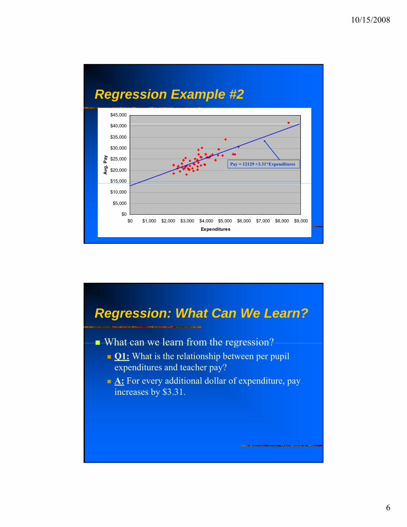
Regression Example #2
Suppose that we are interested inSuppose that we are interested in understanding the determinants of teacher pay.What we have is a data set on average per-pupil expenditures and average teacher pay by state…

10/15/2008
4
Regression Example #2Descriptive Statistics: pay, expenditures
Variable N Mean Median TrMean StDev SE Meanpay 51 24356 23382 23999 4179 585expendit 51 3697 3554 3596 1055 148
Variable Minimum Maximum Q1 Q3pay 18095 41480 21419 26610expendit 2297 8349 2967 4123
Regression Example #2
Covariances: pay, expenditures
pay expenditpay 17467605expendit 3679754 1112520
Correlations: pay, expenditures
Pearson correlation of pay and expenditures = 0.835P-Value = 0.000

10/15/2008
5
Regression Example #2$45,000
$
$20,000
$25,000
$30,000
$35,000
$40,000
Avg.
Pay
$0
$5,000
$10,000
$15,000
$0 $1,000 $2,000 $3,000 $4,000 $5,000 $6,000 $7,000 $8,000 $9,000
Expenditures
Regression Example #2The regression equation is
pay = 12129 + 3.31 expenditures
Predictor Coef SE Coef T PConstant 12129 1197 10.13 0.000expendit 3.3076 0.3117 10.61 0.000S = 2325 R-Sq = 69.7% R-Sq(adj) = 69.1%
pay = 12129 + 3.31 expenditures is the equation of a line and we can add it to our plot of the data.
10/15/2008
6
Regression Example #2
$
$45,000
$15,000
$20,000
$25,000
$30,000
$35,000
$40,000
Avg.
Pay
Pay = 12129 +3.31*Expenditures
$0
$5,000
$10,000
$0 $1,000 $2,000 $3,000 $4,000 $5,000 $6,000 $7,000 $8,000 $9,000
Expenditures
Regression: What Can We Learn?
What can we learn from the regression?What can we learn from the regression?Q1: What is the relationship between per pupil expenditures and teacher pay?A: For every additional dollar of expenditure, pay increases by $3.31.
10/15/2008
7
Regression: What Can We Learn?
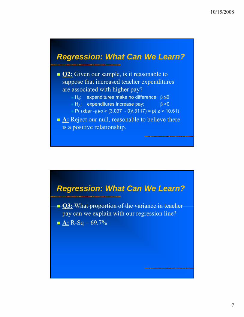
Q2: Given our sample is it reasonable toQ2: Given our sample, is it reasonable to suppose that increased teacher expenditures are associated with higher pay?
H0: expenditures make no difference: β ≤0HA: expenditures increase pay: β >0P( (xbar μ)/σ > (3 037 0)/ 3117) = p( z > 10 61)P( (xbar -μ)/σ > (3.037 - 0)/.3117) = p( z > 10.61)
A: Reject our null, reasonable to believe there is a positive relationship.
Regression: What Can We Learn?
Q3: What proportion of the variance in teacherQ3: What proportion of the variance in teacher pay can we explain with our regression line?A: R-Sq = 69.7%
10/15/2008
8
Regression: What Can We Learn?
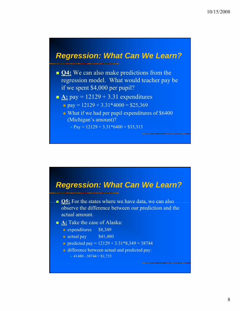
Q4: We can also make predictions from theQ4: We can also make predictions from the regression model. What would teacher pay be if we spent $4,000 per pupil?A: pay = 12129 + 3.31 expenditures
pay = 12129 + 3.31*4000 = $25,369What if we had per pupil expenditures of $6400 (Michigan’s amount)?
Pay = 12129 + 3.31*6400 = $33,313
Regression: What Can We Learn?
Q5: For the states where we have data we can alsoQ5: For the states where we have data, we can also observe the difference between our prediction and the actual amount. A: Take the case of Alaska:
expenditures $8,349actual pay $41,480actual pay $41,480predicted pay = 12129 + 3.31*8,349 = 38744difference between actual and predicted pay:
41480 - 38744 = $1,735
10/15/2008
9
Regression: What Can We Learn?
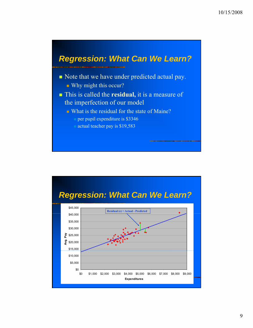
Note that we have under predicted actual payNote that we have under predicted actual pay.Why might this occur?
This is called the residual, it is a measure of the imperfection of our model
What is the residual for the state of Maine?per pupil expenditure is $3346actual teacher pay is $19,583
Regression: What Can We Learn?
$
$45,000Residual (e) = Actual - Predicted
$15,000
$20,000
$25,000
$30,000
$35,000
$40,000
Avg.
Pay
$0
$5,000
$10,000
$0 $1,000 $2,000 $3,000 $4,000 $5,000 $6,000 $7,000 $8,000 $9,000
Expenditures

10/15/2008
10
Regression Nomenclature
Slope CoefficientIntercept
Y=$0+$1*X+,Dependent Variable Explanatory Variable Residual or Error
p
i ii
i indexes the observation
Pay=12,129 + 3.31*Expenditure + e
Slope CoefficientIntercept
i i i
10/15/2008
11
Components of a Regression Model
Dependent variable: we are trying to explain theDependent variable: we are trying to explain the movement of the dependent variable around its mean.Explanatory variable(s): We use these variables to explain the movement of the dependent variable.Error Term: This is the difference between what we can account for with our explanatory variables and th t l l t k b th d d t i blthe actual value taken on by the dependent variable.Parameter: The measure of the relationship between an explanatory variable and a dependent variable.
Regression Models are Linear
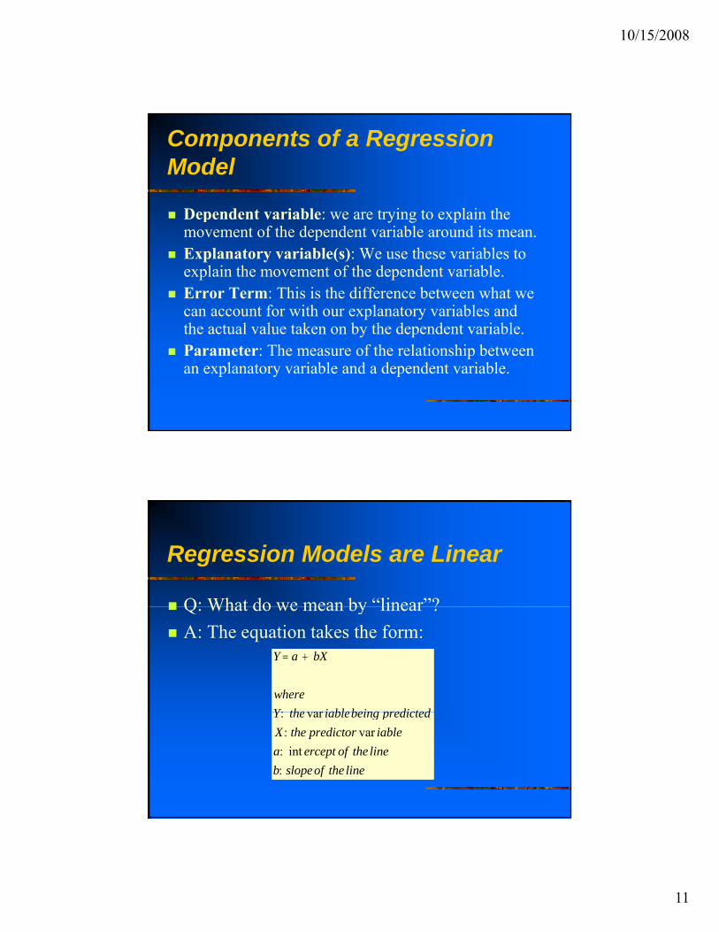
Q: What do we mean by “linear”?Q: What do we mean by linear ?A: The equation takes the form:
Y a bX
whereY the iablebeing predicted
= +
: varY the iablebeing predictedX the predictor iablea ercept of the lineb slopeof the line
: var: var
: int:
10/15/2008
12
Regression Example #3
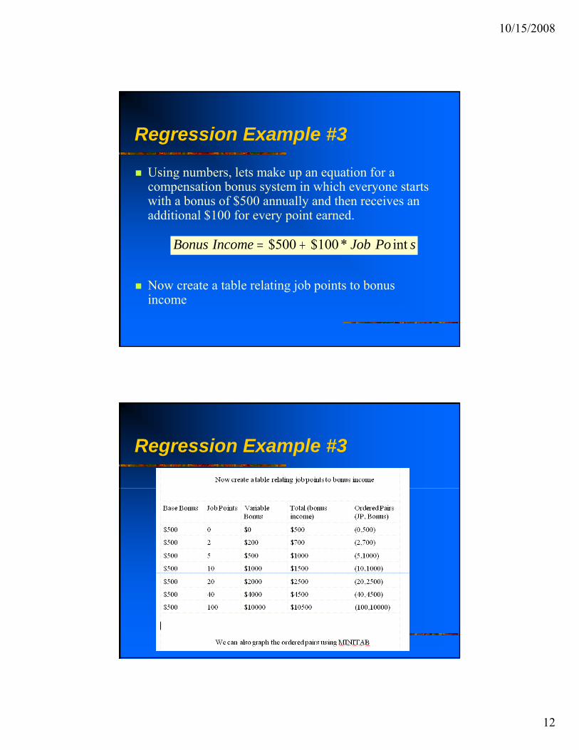
Using numbers, lets make up an equation for aUsing numbers, lets make up an equation for a compensation bonus system in which everyone starts with a bonus of $500 annually and then receives an additional $100 for every point earned.
Bonus Income Job Po s= +$500 $100* int
Now create a table relating job points to bonus income
Regression Example #3

10/15/2008
13
Regression Example #3
Regression Example #3
Basic model takes the form:Basic model takes the form:
Y = β0 + β1*X + ε
or, for the bonus pay example,
Pay = $500 + $100*expenditure + ε
10/15/2008
14
Regression Example #3
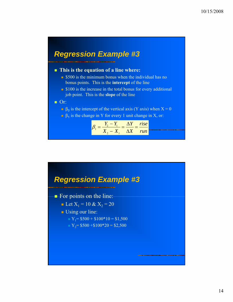
This is the equation of a line where:This is the equation of a line where:$500 is the minimum bonus when the individual has no bonus points. This is the intercept of the line$100 is the increase in the total bonus for every additional job point. This is the slope of the line
Or:β0 is the intercept of the vertical axis (Y axis) when X = 0β1 is the change in Y for every 1 unit change in X, or:
β12 1
2 1
=−−
= =Y YX X
YX
riserun
ΔΔ
Regression Example #3
For points on the line:For points on the line:Let X1 = 10 & X2 = 20Using our line:
Y1= $500 + $100*10 = $1,500Y2= $500 +$100*20 = $2,500

10/15/2008
15
Regression Example #3
Regression Example #3
1 The change in bonus pay for a 1 point1. The change in bonus pay for a 1 point increase in job points:
2 What do we mean by “linear”?
β1
500 50020 10
00010
=−−
= =$2, $1, $1, $100
2. What do we mean by linear ?Equation of a line:Y = β0 + β1*X + ε is the equation of a line

10/15/2008
16
Regression Example #3
Equation of a line which is linear in coefficients butEquation of a line which is linear in coefficients but not variables:
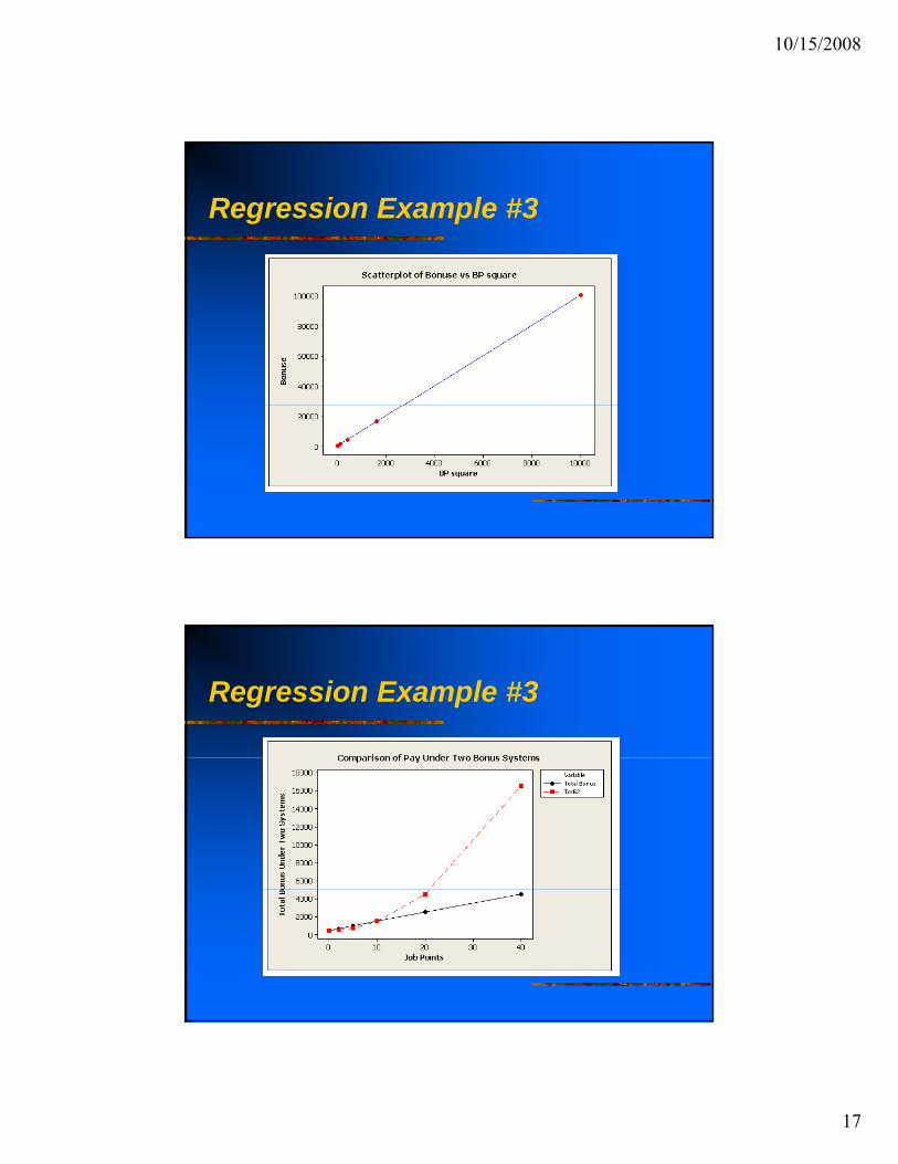
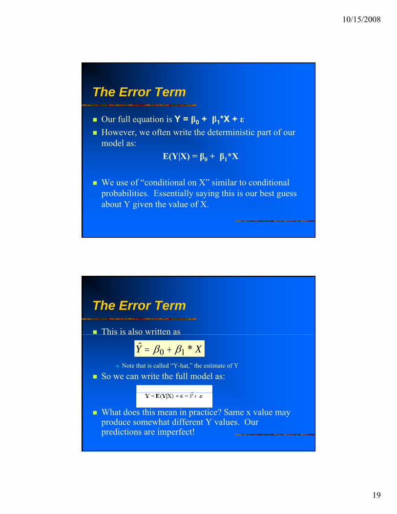
Y = β0 + β1*X + β2*X2 + εThink about a new bonus equation:
Total Bonus Bonus Po s Bonus Po s= + +500 0 10 2* int * int
Base Bonus is still $500You now get $0 per bonus point and $10 per bonus point squared
Regression Example #3
10/15/2008
17
Regression Example #3
Regression Example #3

10/15/2008
18
Linearity of Regression Models
Y = β + β *Xβ + ε is not the equation of aY = β0 + β2 Xβ + ε is not the equation of a lineRegression has to be linear in coefficients, not variablesWe can mimic curves and much else if we are clever
The Error Term
The error term is the difference between what hasThe error term is the difference between what has occurred and what we predict as an outcome.Our models are imperfect because
omitted “minor” influencesmeasurement error in Y and X’sissues of functional form (linear model for non-linearissues of functional form (linear model for non linear relationship)pure randomness of behavior
10/15/2008
19
The Error Term
Our full equation is Y = β0 + β1*X + εOur full equation is Y β0 + β1 X + εHowever, we often write the deterministic part of our model as:
E(Y|X) = β0 + β1*X
W f “ di i l X” i il di i lWe use of “conditional on X” similar to conditional probabilities. Essentially saying this is our best guess about Y given the value of X.
The Error Term
This is also written asThis is also written as
Note that is called “Y-hat,” the estimate of Y
So we can write the full model as:
$ *Y X= +β β0 1
What does this mean in practice? Same x value may produce somewhat different Y values. Our predictions are imperfect!
10/15/2008
20
Populations, Samples, and Regression Analysis
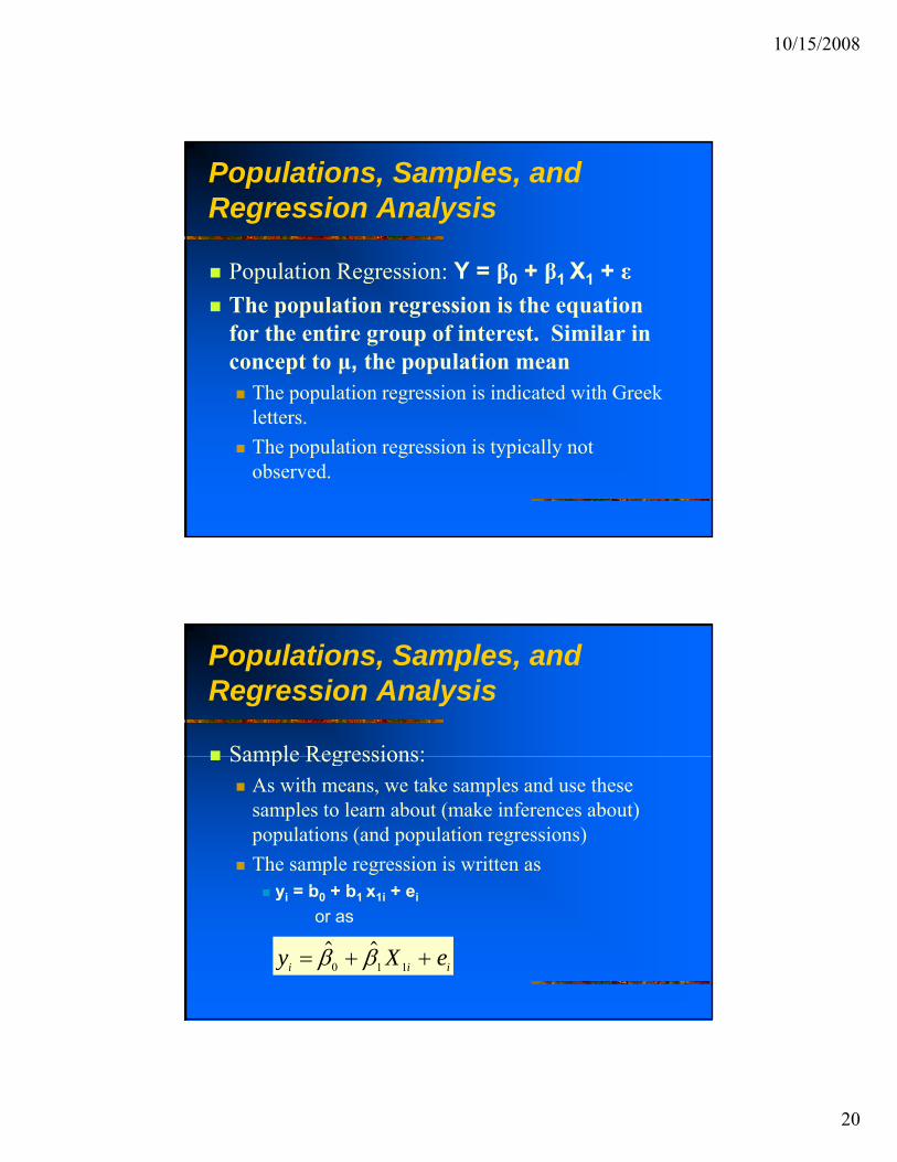
Population Regression: Y = β + β X + εPopulation Regression: Y = β0 + β1 X1 + εThe population regression is the equation for the entire group of interest. Similar in concept to μ, the population mean
The population regression is indicated with Greek letters.The population regression is typically not observed.
Populations, Samples, and Regression Analysis
Sample Regressions:Sample Regressions:As with means, we take samples and use these samples to learn about (make inferences about) populations (and population regressions)The sample regression is written as
y = b + b x + eyi = b0 + b1 x1i + ei
or as
y X ei i i= + +$ $β β0 1 1

10/15/2008
21
Populations, Samples, and Regression Analysis
Populations, Samples, and Regression Analysis
As with all sample results there are lots ofAs with all sample results, there are lots of samples which might be drawn from a population. These samples will typically provide somewhat different estimates of the coefficients. This is, once more, sampling
i ivariation.

10/15/2008
22
Populations and Samples: Regression Example
Illustrative Exercise:Illustrative Exercise:1. Estimate a simple regression model for all of the data on managers and professionals, then take random 10% subsamples of the data and compare the estimates!2. Sample estimates are generated by assigning a number between 0 and 1 to every observation using a uniform distribution We then chose observations for all of thedistribution. We then chose observations for all of the numbers betwee 0 and 0.1, 0.1 and 0.2, 0.3 and 0.3, etc.
Populations and Samples: Regression ExamplePOPULATION ESTIMATES: Results for: lir832-managers-and-
professionals-2000.mtw
The regression equation isweekearn = - 485 + 87.5 years ed
47576 cases used 7582 cases contain missing values
Predictor Coef SE Coef T PConstant -484.57 18.18 -26.65 0.000years ed 87.492 1.143 76.54 0.000years ed 87.492 1.143 76.54 0.000
S = 530.5 R-Sq = 11.0% R-Sq(adj) = 11.0%
Analysis of VarianceSource DF SS MS F PRegression 1 1648936872 1648936872 5858.92 0.000Residual Error 47574 13389254994 281441Total 47575 15038191866

10/15/2008
23
Side Note: Reading OutputThe regression equation isweekearn = - 485 + 87.5 years ed [equation with dependent
variable]
47576 cases used 7582 cases contain missing values [number of observations and number with missing data - why is the
latter important]
Predictor Coef SE Coef T PConstant -484.57 18.18 -26.65 0.000years ed 87.492 1.143 76.54 0.000[detailed information on estimated coefficients, standard error,
t against a null of zero, and a p against a null of 0]
S = 530.5 R-Sq = 11.0% R-Sq(adj) = 11.0% [two goodness of fit measures]
Side Note: Reading OutputAnalysis of Variance
Source DF SS MS F P
Regression 1 1648936872 1648936872 5858.92 0.000 ESSResidual Error 47574 13389254994 281441 SSRTotal 47575 15038191866 TSS
[This tells us the number of degrees of freedom, the explained sum of[This tells us the number of degrees of freedom, the explained sum of squares, the residual sum of squares, the total sum of squares and some test statistics]

10/15/2008
24
Populations and Samples: Regression Example
Populations and Samples: Regression ExampleSAMPLE 1 RESULTS
The regression equation isweekearn = - 333 + 79.2 Education
4719 cases used 726 cases contain missing values
Predictor Coef SE Coef T PConstant -333.24 58.12 -5.73 0.000Educatio 79.208 3.665 21.61 0.000
S = 539.5 R-Sq = 9.0% R-Sq(adj) = 9.0%

10/15/2008
25
Populations and Samples: Regression Example
Populations and Samples: Regression ExampleSAMPLE 2 RESULTS
The regression equation isweekearn = - 489 + 88.2 Education
4792 cases used 741 cases contain missing values
Predictor Coef SE Coef T PConstant -488.51 56.85 -8.59 0.000Educatio 88.162 3.585 24.59 0.000
S = 531.7 R-Sq = 11.2% R-Sq(adj) = 11.2%
10/15/2008
26
Populations and Samples: Regression Example
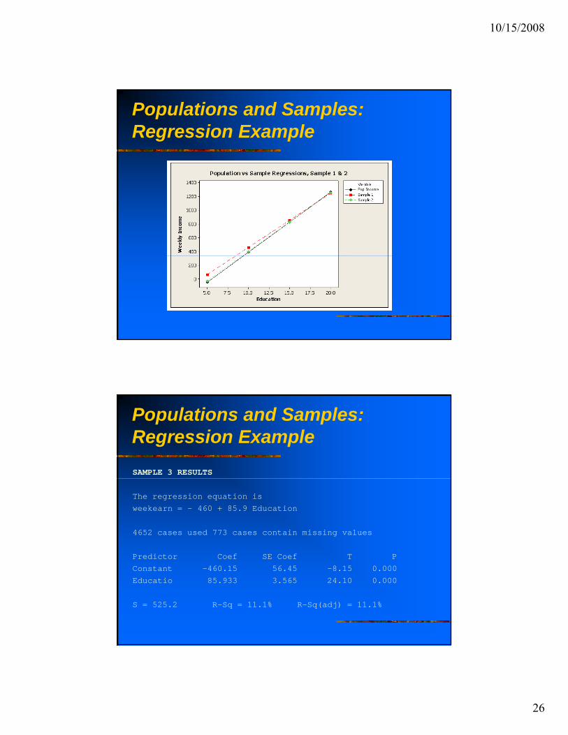
Populations and Samples: Regression ExampleSAMPLE 3 RESULTS
The regression equation isweekearn = - 460 + 85.9 Education
4652 cases used 773 cases contain missing values
Predictor Coef SE Coef T PConstant -460.15 56.45 -8.15 0.000Educatio 85.933 3.565 24.10 0.000
S = 525.2 R-Sq = 11.1% R-Sq(adj) = 11.1%
10/15/2008
27
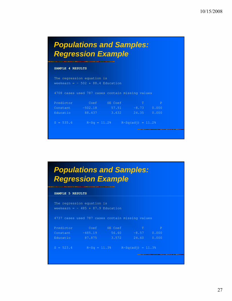
Populations and Samples: Regression ExampleSAMPLE 4 RESULTS
The regression equation isweekearn = - 502 + 88.4 Education
4708 cases used 787 cases contain missing values
Predictor Coef SE Coef T PConstant -502.18 57.51 -8.73 0.000Educatio 88.437 3.632 24.35 0.000
S = 535.6 R-Sq = 11.2% R-Sq(adj) = 11.2%
Populations and Samples: Regression ExampleSAMPLE 5 RESULTS
The regression equation isweekearn = - 485 + 87.9 Education
4737 cases used 787 cases contain missing values
Predictor Coef SE Coef T PConstant -485.19 56.60 -8.57 0.000Educatio 87.875 3.572 24.60 0.000
S = 523.4 R-Sq = 11.3% R-Sq(adj) = 11.3%

10/15/2008
28
Populations and Samples: Regression Example
Populations and Samples: A Recap of the Example
Estimate β0 (Intercept)β1 (Coefficient on Education)
POPULATION -484.57 87.49Sample 1 -333.24 79.21Sample 2 488 51 88 16Sample 2 -488.51 88.16Sample 3 -460.15 85.93Sample 4 -502.18 88.44Sample 5 -485.19 87.88

10/15/2008
29
Populations and Samples: A Recap of the Example
The sample estimates are not exactly equal toThe sample estimates are not exactly equal to the population estimates.Different samples produce different estimates of the slope and intercept.
Ordinary Least Squares (OLS): How We Determine the Estimates
The residual is a measure of what we do not know.The residual is a measure of what we do not know.ei = yi - b0 + b1 x1iWe want ei to be as small as possible
How do we choose (b0, b1)? AKA: Criteria for the sample regression:
Chose among lines so that: Th l f th id l i
eii
n=
=∑ 0
1
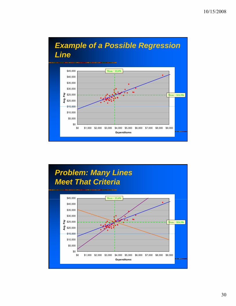
The average value of the residual is zero.Statistically, this occurs through any line that passes through the means (X-bar, Y-bar).Problem: there are an infinity of lines which meet this criteria.
10/15/2008
30
Example of a Possible Regression Line
$45,000 Mean = $3,696
$15 000
$20,000
$25,000
$30,000
$35,000
$40,000
$ ,
Avg.
Pay Mean = $24,356
,
$0
$5,000
$10,000
$15,000
$0 $1,000 $2,000 $3,000 $4,000 $5,000 $6,000 $7,000 $8,000 $9,000
Expenditures
Problem: Many Lines Meet That Criteria
$45,000 Mean = $3,696
$15 000
$20,000
$25,000
$30,000
$35,000
$40,000
$ ,
Avg.
Pay Mean = $24,356
,
$0
$5,000
$10,000
$15,000
$0 $1,000 $2,000 $3,000 $4,000 $5,000 $6,000 $7,000 $8,000 $9,000
Expenditures
10/15/2008
31
OLS: Choosing the Coefficients
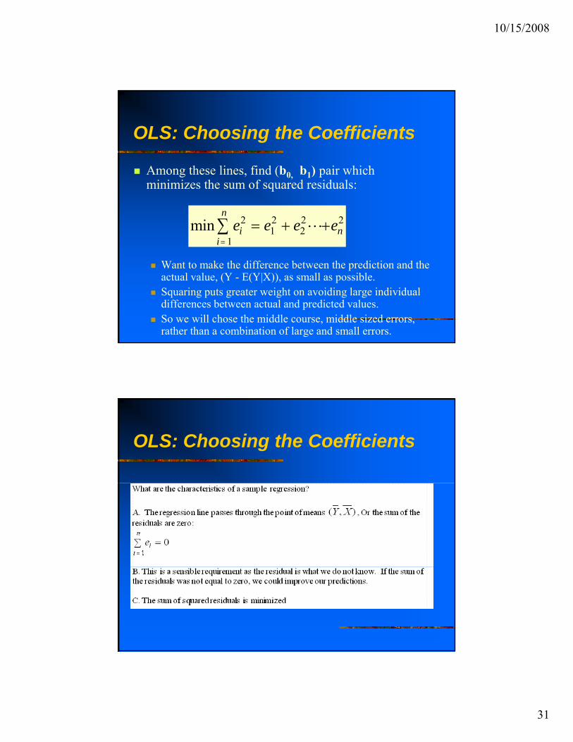
Among these lines, find (b0 b1) pair whichAmong these lines, find (b0, b1) pair which minimizes the sum of squared residuals:
min e e e eii
n
n2
112
22 2
=∑ = + +L
Want to make the difference between the prediction and the actual value, (Y - E(Y|X)), as small as possible.Squaring puts greater weight on avoiding large individual differences between actual and predicted values.So we will chose the middle course, middle sized errors, rather than a combination of large and small errors.
OLS: Choosing the Coefficients
10/15/2008
32
OLS: Choosing the Coefficients
What are the characteristics of a sample regression?What are the characteristics of a sample regression?D. It can be shown that, if these two conditions hold, our regression line is:
BestLinearUnbiasedUnbiasedEstimator (or B-L-U-E)
This is called the: Gauss-Markov Theorem
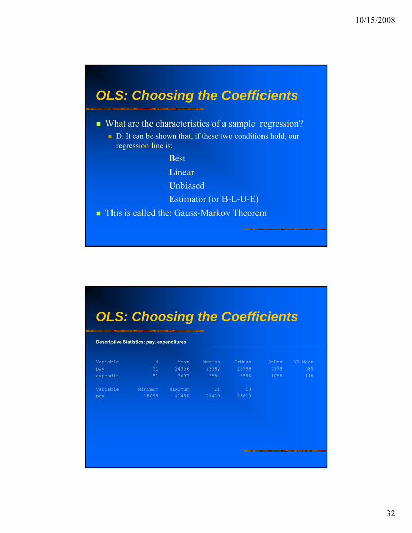
OLS: Choosing the CoefficientsDescriptive Statistics: pay, expenditures
Variable N Mean Median TrMean StDev SE Meanpay 51 24356 23382 23999 4179 585expendit 51 3697 3554 3596 1055 148
Variable Minimum Maximum Q1 Q3pay 18095 41480 21419 26610
10/15/2008
33
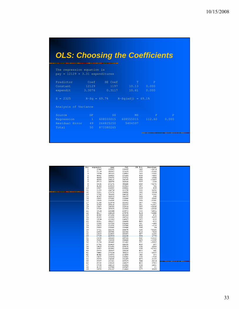
OLS: Choosing the CoefficientsThe regression equation ispay = 12129 + 3.31 expenditures
Predictor Coef SE Coef T PConstant 12129 1197 10.13 0.000expendit 3.3076 0.3117 10.61 0.000
S = 2325 R-Sq = 69.7% R-Sq(adj) = 69.1%
Analysis of Variancey
Source DF SS MS F PRegression 1 608555015 608555015 112.60 0.000Residual Error 49 264825250 5404597Total 50 873380265

10/15/2008
34
OLS: Choosing the Coefficients
Mean of the residuals equal to zero?ea o t e es dua s equa to e o
Descriptive Statistics: Residual
Variable N Mean Median TrMean StDev SE MeanResidual 51 -0 -218 -107 2301 322
Variable Minimum Maximum Q1 Q3Residual -3848 5529 -2002 1689
OLS: Choosing the CoefficientsPasses Through the Point of Means?
pay = 12129 + 3.3076 expenditures
Variable N Mean pay 51 24356 expendit 51 3697
$24,356 = 12129 + 3.3076*3697
$24,356 = 12129 + 12,122.20
$24,356 = $24357.2 Not too bad with rounding!
10/15/2008
35
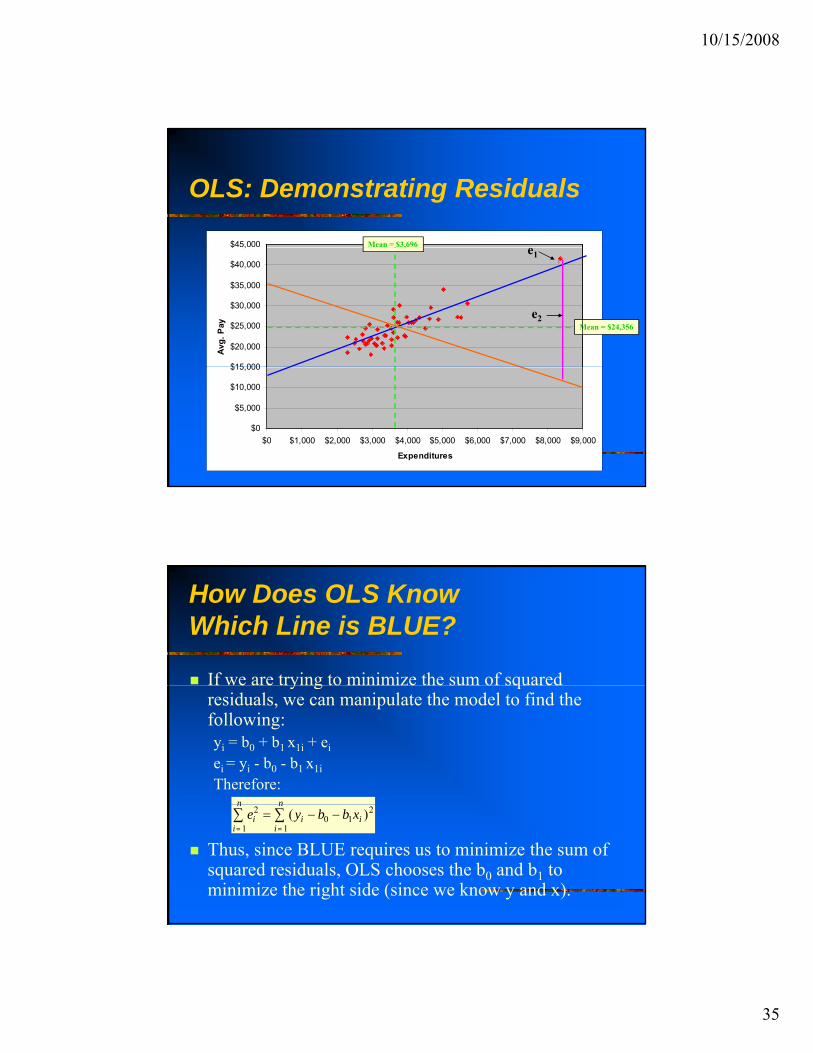
OLS: Demonstrating Residuals
$45,000 Mean = $3,696
$15 000
$20,000
$25,000
$30,000
$35,000
$40,000
$ ,
Avg.
Pay Mean = $24,356
, e1
e2
$0
$5,000
$10,000
$15,000
$0 $1,000 $2,000 $3,000 $4,000 $5,000 $6,000 $7,000 $8,000 $9,000
Expenditures
How Does OLS Know Which Line is BLUE?
If we are trying to minimize the sum of squaredIf we are trying to minimize the sum of squared residuals, we can manipulate the model to find the following:yi = b0 + b1 x1i + eiei = yi - b0 - b1 x1iTherefore:
n n
Thus, since BLUE requires us to minimize the sum of squared residuals, OLS chooses the b0 and b1 to minimize the right side (since we know y and x).
e y b b xii
n
ii
n
i2
10
11
2
= =∑ ∑= − −( )

10/15/2008
36
How Does OLS Calculate the Coefficients?
The formulas used for the coefficients are asThe formulas used for the coefficients are as follows:
byx
x yx
x x y yx x
xy
x
i i
ii
n
1 2 21
= = = =− −
−=∑Δ
Δcov( , )
var( )( )( )
( )σσ
b y b x0 1= −
Illustrative Example: Attendance and Output
Attendance Output8 40
We want to build a model of output based on attendance. We hypothesize the following:
output = β0 + β1*attendance + ε
8 403 282 206 394 28
10/15/2008
37
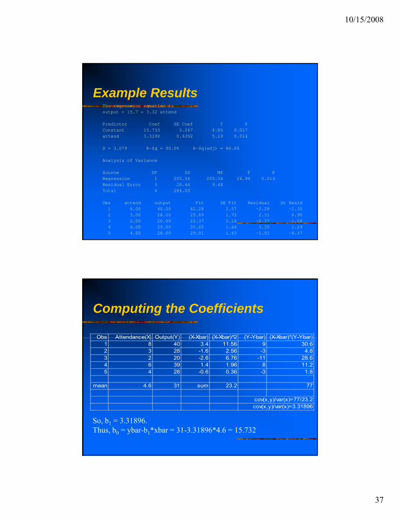
Example ResultsThe regression equation isoutput = 15.7 + 3.32 attend
Predictor Coef SE Coef T PConstant 15.733 3.247 4.85 0.017attend 3.3190 0.6392 5.19 0.014
S = 3.079 R-Sq = 90.0% R-Sq(adj) = 86.6%
Analysis of Variance
Source DF SS MS F PRegression 1 255.56 255.56 26.96 0.014Residual Error 3 28.44 9.48Total 4 284.00
Obs attend output Fit SE Fit Residual St Resid1 8.00 40.00 42.28 2.57 -2.28 -1.35 2 3.00 28.00 25.69 1.72 2.31 0.90 3 2.00 20.00 22.37 2.16 -2.37 -1.08 4 6.00 39.00 35.65 1.64 3.35 1.29 5 4.00 28.00 29.01 1.43 -1.01 -0.37
Computing the Coefficients
Obs Attendance(X) Output(Y) (X-Xbar) (X-Xbar)^2 (Y-Ybar) (X-Xbar)*(Y-Ybar)Obs Attendance(X) Output(Y) (X-Xbar) (X-Xbar) 2 (Y-Ybar) (X-Xbar) (Y-Ybar)1 8 40 3.4 11.56 9 30.62 3 28 -1.6 2.56 -3 4.83 2 20 -2.6 6.76 -11 28.64 6 39 1.4 1.96 8 11.25 4 28 -0.6 0.36 -3 1.8
mean 4.6 31 sum 23.2 77
cov(x,y)/var(x)=77/23.2cov(x,y)/var(x)=3.31896
So, b1 = 3.31896.Thus, b0 = ybar-b1*xbar = 31-3.31896*4.6 = 15.732

10/15/2008
38
Example: Residual AnalysisVariable N Mean Median TrMean StDev SE MeanC15 5 0.00 -1.01 0.00 2.66 1.19
Variable Minimum Maximum Q1 Q3C15 -2.37 3.35 -2.33 2.83
Exercise
We are interested in the relationship between theWe are interested in the relationship between the number of weeks an employee has been in some firm sponsored training course and output. We have data on three employees. Thus, compute the coefficients for the following model:
output = β0 + β1*training + εp β0 β1 g
Weeks Training Outputemployee 1 10 590employee 2 20 400employee 3 30 430
10/15/2008
39
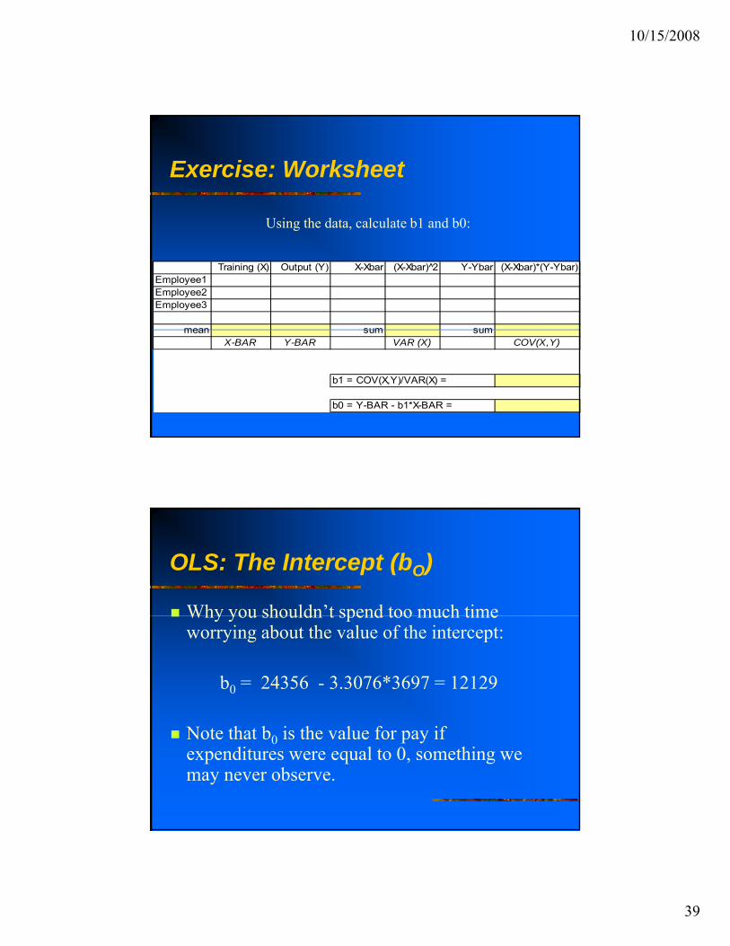
Exercise: Worksheet
Using the data calculate b1 and b0:
Training (X) Output (Y) X-Xbar (X-Xbar) 2̂ Y-Ybar (X-Xbar)*(Y-Ybar)Employee1Employee2Employee3
mean sum sum
Using the data, calculate b1 and b0:
mean sum sumX-BAR Y-BAR VAR (X) COV(X,Y)
b1 = COV(X,Y)/VAR(X) =
b0 = Y-BAR - b1*X-BAR =
OLS: The Intercept (bO)
Why you shouldn’t spend too much timeWhy you shouldn t spend too much time worrying about the value of the intercept:
b0 = 24356 - 3.3076*3697 = 12129
Note that b0 is the value for pay if expenditures were equal to 0, something we may never observe.
10/15/2008
40
Multiple Regression
Few outcomes are determined by a single factor:y g1. We know that gender plays an important role in determining pay. Is gender the only factor? 2. What is likely to matter in determining attendance at a work site:
our programholidaysholidaysweatherillnessdemographics of the labor force
Multiple Regression
A complete model of an outcome will dependA complete model of an outcome will depend not only on inclusion of our explanatory variable of interest, but also including other variables which we believe influence our outcome.
Getting the “correct” estimates of our coefficients depends on specifying the balance of the equation correctly. This raises the bar in our work.
10/15/2008
41
Multiple Regression: Example
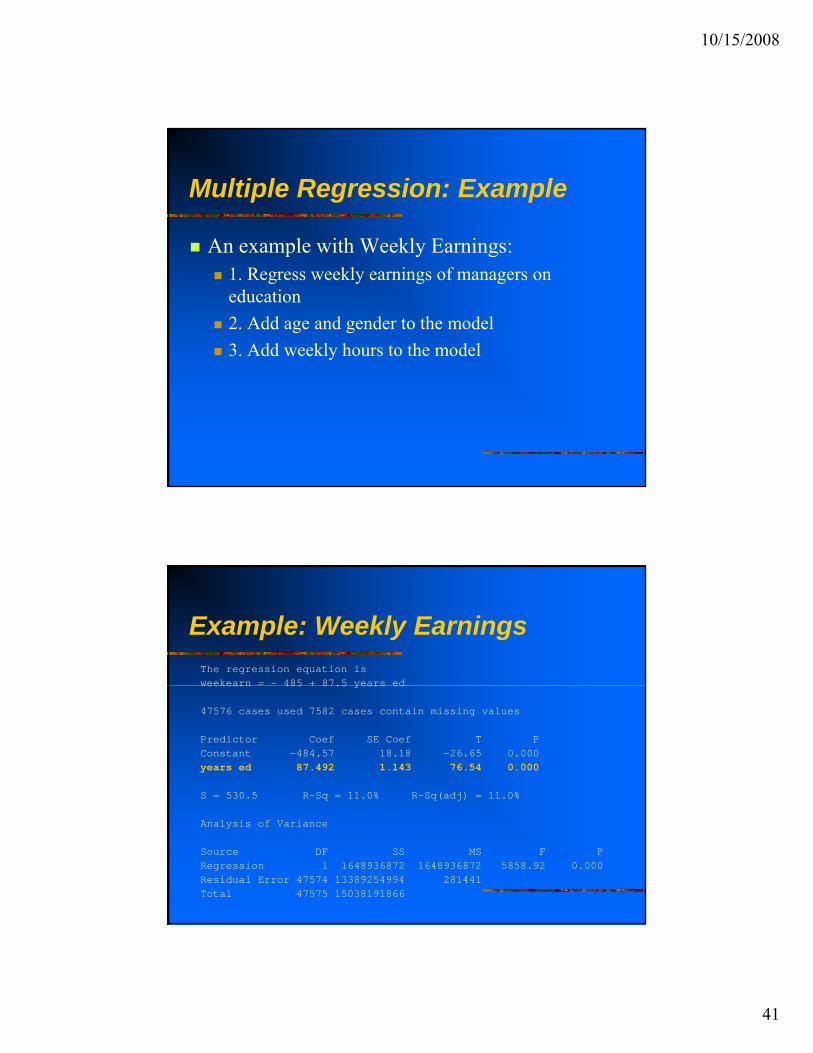
An example with Weekly Earnings:An example with Weekly Earnings:1. Regress weekly earnings of managers on education2. Add age and gender to the model3. Add weekly hours to the model
Example: Weekly EarningsThe regression equation isweekearn = - 485 + 87.5 years edweekearn 485 + 87.5 years ed
47576 cases used 7582 cases contain missing values
Predictor Coef SE Coef T PConstant -484.57 18.18 -26.65 0.000years ed 87.492 1.143 76.54 0.000
S = 530.5 R-Sq = 11.0% R-Sq(adj) = 11.0%
Analysis of Variance
Source DF SS MS F PRegression 1 1648936872 1648936872 5858.92 0.000Residual Error 47574 13389254994 281441Total 47575 15038191866
10/15/2008
42
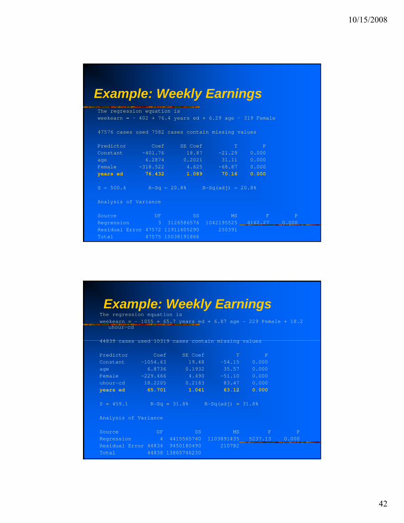
Example: Weekly EarningsThe regression equation isweekearn = - 402 + 76.4 years ed + 6.29 age - 319 Female
47576 cases used 7582 cases contain missing values
Predictor Coef SE Coef T PConstant -401.76 18.87 -21.29 0.000age 6.2874 0.2021 31.11 0.000Female -318.522 4.625 -68.87 0.000years ed 76.432 1.089 70.16 0.000
S = 500.4 R-Sq = 20.8% R-Sq(adj) = 20.8%
Analysis of Variance
Source DF SS MS F PRegression 3 3126586576 1042195525 4162.27 0.000Residual Error 47572 11911605290 250391Total 47575 15038191866
Example: Weekly EarningsThe regression equation isweekearn = - 1055 + 65.7 years ed + 6.87 age - 229 Female + 18.2
uhour-cd
44839 cases sed 10319 cases contain missing al es44839 cases used 10319 cases contain missing values
Predictor Coef SE Coef T PConstant -1054.63 19.48 -54.15 0.000age 6.8736 0.1932 35.57 0.000Female -229.466 4.490 -51.10 0.000uhour-cd 18.2205 0.2183 83.47 0.000years ed 65.701 1.041 63.12 0.000
S = 459.1 R-Sq = 31.8% R-Sq(adj) = 31.8%
Analysis of Variance
Source DF SS MS F PRegression 4 4415565740 1103891435 5237.13 0.000Residual Error 44834 9450180490 210782Total 44838 13865746230

10/15/2008
43
Example: Weekly Earnings
In the last model how does age affect weeklyIn the last model, how does age affect weekly earnings? How does gender affect weekly earnings? How do average weekly hours of work affect weekly earnings?How does the estimated effect of education change as we add these “control variables”?
Interpreting the Coefficients
In the last model, the coefficient on education indicates that ,for every additional year of education a manager earnings an additional 65.09 per month, holding their age, gender, and hours of work constant.
E(Weekly Income|education,age, gender, hours of work)
Alternatively it is the difference in weekly earnings betweenAlternatively, it is the difference in weekly earnings between two individuals who, except for a one year difference in years of education, are the same age and gender and work the same weekly hours (otherwise equivalent managers)

10/15/2008
44
Interpreting the Coefficients
The coefficient on gender indicates that women managers earn g g$229.79 less than male managers who are otherwise similar in education, age and weekly hours of work.Note the similarity to the comparative static exercises in labor economics in which we attempt to tease out the effect of one factor holding all other factors constant.
What is the effect of raising the demand for labor, holding supply of g , g pp ylabor constant?What is the effect on the wage of an improvement in working conditions, holding other compensation related factors constant (Theory of compensating differentials).
The Effect of Adding Variables
The addition of factors to a model don’tThe addition of factors to a model don t always make a difference.
Example: Model of teacher pay as a function of expenditures per pupil. Does region make a difference.
10/15/2008
45
The Effect of Adding Variables
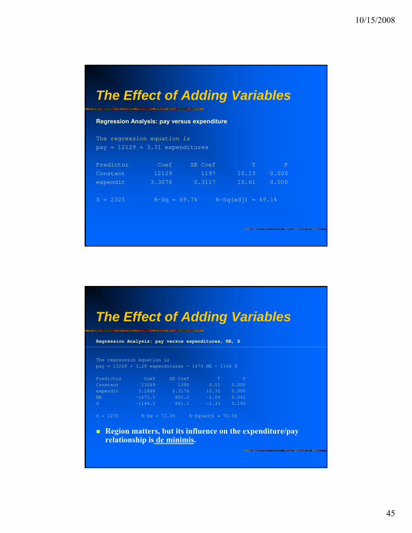
Regression Analysis: pay versus expenditure
The regression equation ispay = 12129 + 3.31 expenditures
Predictor Coef SE Coef T PConstant 12129 1197 10.13 0.000expendit 3.3076 0.3117 10.61 0.000
S = 2325 R-Sq = 69.7% R-Sq(adj) = 69.1%
The Effect of Adding VariablesRegression Analysis: pay versus expenditures, NE, S
The regression equation ispay = 13269 + 3.29 expenditures - 1674 NE - 1144 S
Predictor Coef SE Coef T PConstant 13269 1395 9.51 0.000expendit 3.2888 0.3176 10.35 0.000NE -1673.5 801.2 -2.09 0.042S -1144.2 861.1 -1.33 0.190
S = 2270 R-Sq = 72.3% R-Sq(adj) = 70.5%
Region matters, but its influence on the expenditure/pay relationship is de minimis.

10/15/2008
46
Evaluating the Results
We will consider a number of criteria inWe will consider a number of criteria in analyzing a regression equation.
Before touching the dataIs the equation supported by sound theory?Are all the obviously important variables included in the model?model?Should we be using OLS to estimate this Model (what is OLS)?Has the correct form been used to estimate the model?
Evaluating the Results
The data itself:The data itself:Is the data set a reasonable size and accurate?
The results:How well does the estimated regression fit the data?Do the estimated coefficients correspond to the expectations developed by the researcher before the p p ydata was collected?Does the regression appear to be free of major econometric problems?

10/15/2008
47
Evaluating the Results: R-Squared (Goodness of Fit)
R2 (also seen as r2) the Coefficient ofR (also seen as r ), the Coefficient of Determination:
We would like a simple measure which tells us how well our equation fits out data. This is R2 ( Coefficient of Determination)For example: in our teacher pay model: R2 = 69.7%For attendance/output: R2 = 86.6%For our weekly earnings model R2 varies from 10.6% to 31.9%
R-Squared (Goodness of Fit)
What is R2? The percentage of the totalWhat is R ? The percentage of the total movement of the dependent variable around its mean (variance *n) explained by the explanatory variable.
10/15/2008
48
R-Squared (Goodness of Fit)
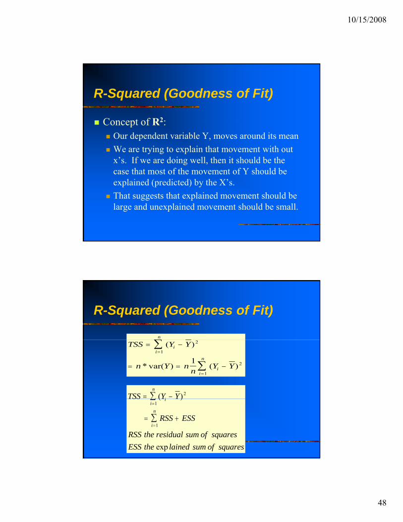
Concept of R2:Concept of R :Our dependent variable Y, moves around its mean We are trying to explain that movement with out x’s. If we are doing well, then it should be the case that most of the movement of Y should be explained (predicted) by the X’sexplained (predicted) by the X s. That suggests that explained movement should be large and unexplained movement should be small.
R-Squared (Goodness of Fit)
n
∑TSS Y Y
n Y nn
Y Y
ii
ii
n
= −
= = −
=
=
∑
∑
( )
* var( ) ( )
2
1
2
1
1
TSS Y Yi
n
= −∑ ( )2SS
RSS ESS
RSS the residual sum of squaresESS the lained sum of squares
ii
i
n
= +
=
=
∑
∑
( )
exp
1
1

10/15/2008
49
R-Squared (Goodness of Fit)
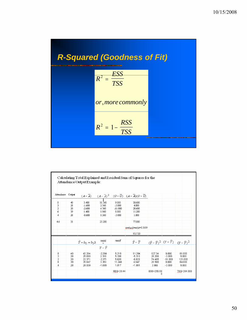
R ESS lained sum of squares2 = =exp
Note: 0 < R2 < 1Suppose that we a regression which explains nothing. Then the ESS = 0 and the measure is equal to zero.
RTSS total sum of squares
= =
Now suppose we have a model which fits the data exactly. Every movement in y is correctly predicted. Then the ESS = TSS and our measure is equal to 1.
R-Squared (Goodness of Fit)
In other words as we approach R2=1 ourIn other words, as we approach R =1, our ability to explain movement in the dependent variable increases.
Most of our results will fall into the middle range between 0 and 1.
10/15/2008
50
R-Squared (Goodness of Fit)
ESS2RESSTSS
or morecommonly
2 =
,
RRSSTSS
2 1= −

10/15/2008
51
Returning to Weekly Earnings of Managers ExamplesThe regression equation isweekearn = - 485 + 87.5 years ed [equation with
dependent variable]
47576 cases used 7582 cases contain missing values [number of observations and number with missing data - why
is the latter important]
Predictor Coef SE Coef T PConstant -484.57 18.18 -26.65 0.000years ed 87.492 1.143 76.54 0.000[detailed information on estimated coefficients, standard
error, t against a null of zero, and a p against a null of 0]
S = 530.5 R-Sq = 11.0% R-Sq(adj) = 11.0% [two goodness of fit measures]
Returning to Weekly Earnings of Managers ExamplesRegression Analysis: weekearn versus Education
The regression equation isweekearn = - 442 + 85.2 Education
47576 cases used 7582 cases contain missing values
Predictor Coef SE Coef T PConstant -442.42 17.99 -24.59 0.000Educatio 85.228 1.136 75.01 0.000
S = 531.7 R-Sq = 10.6% R-Sq(adj) = 10.6%
Analysis of Variance
Source DF SS MS F PRegression 1 1590256151 1590256151 5625.76 0.000Residual Error 47574 13447935715 282674Total 47575 15038191866

10/15/2008
52
Returning to Weekly Earnings of Managers ExamplesRegression Analysis: weekearn versus Education, age, female
The regression equation isweekearn = - 382 + 75.0 Education + 6.53 age - 320 female
47576 cases used 7582 cases contain missing values
Predictor Coef SE Coef T PConstant -382.38 18.78 -20.36 0.000Educatio 74.967 1.079 69.45 0.000age 6.5320 0.2020 32.34 0.000female -319.952 4.628 -69.14 0.000
S = 500.9 R-Sq = 20.6% R-Sq(adj) = 20.6%
Analysis of Variance
Source DF SS MS F PRegression 3 3103974768 1034658256 4124.34 0.000Residual Error 47572 11934217098 250866Total 47575 15038191866
Returning to Weekly Earnings of Managers ExamplesRegression Analysis: weekearn versus Education, age, female, hours
The regression equation isweekearn = - 1053 + 65.1 Education + 7.07 age - 230 female + 18.3
hours
44839 cases used 10319 cases contain missing values
Predictor Coef SE Coef T PConstant -1053.01 19.43 -54.20 0.000Educatio 65.089 1.029 63.27 0.000age 7.0741 0.1929 36.68 0.000female -229.786 4.489 -51.19 0.000hours 18.3369 0.2180 84.11 0.000
S = 459.0 R-Sq = 31.9% R-Sq(adj) = 31.9%
10/15/2008
53
Returning to Weekly Earnings of Managers Examples
So the fit of the final model with a control forSo the fit of the final model, with a control for hours of work, is considerably better than the fit for a model which added gender and age and much better than the fit of a model with just education as an explanatory variable.
Adjusted R-Squared (“R-bar Squared”)
First limitation of R2:First limitation of R1. As we add variables, the magnitude of ESS never falls and typically increases. If we just use R2 as a criteria for adding variables to a model, we will keep adding infinitum. R2 never falls and usually increases as one adds variablesusually increases as one adds variables.2. Instead use the measure R-bar squared. This measure is calculated as:
10/15/2008
54
Adjusted R-Squared (“R-bar Squared”)
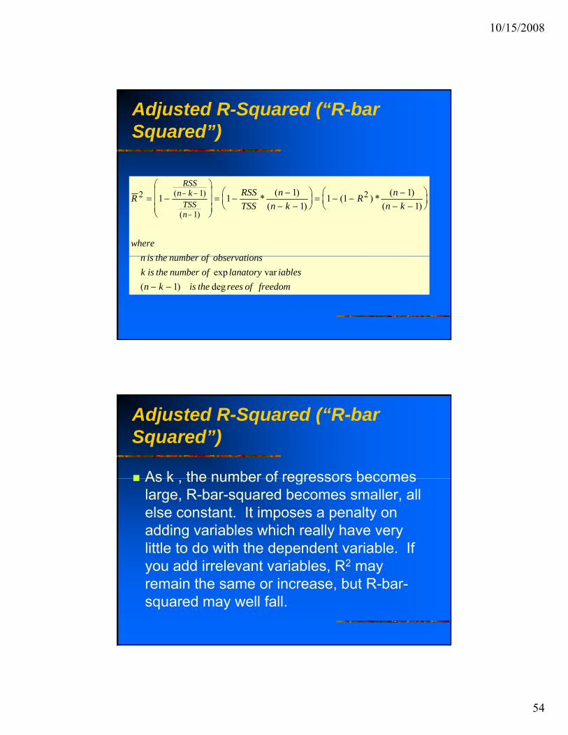
R RSSTSS
nn k
R nn k
wherei th b f b ti
RSSn k
TSSn
2 1
1
21 1 11
1 1 11
= −⎛
⎝
⎜⎜⎜
⎞
⎠
⎟⎟⎟= −
−− −
⎛⎝⎜
⎞⎠⎟ = − −
−− −
⎛⎝⎜
⎞⎠⎟
− −
−
( )
( )
* ( )( )
( ) * ( )( )
n is the number of observationsk is the number of lanatory iablesn k is the rees of freedom1− −
exp var( ) deg
Adjusted R-Squared (“R-bar Squared”)
As k the number of regressors becomesAs k , the number of regressors becomes large, R-bar-squared becomes smaller, all else constant. It imposes a penalty on adding variables which really have very little to do with the dependent variable. If
dd i l t i bl R2you add irrelevant variables, R2 may remain the same or increase, but R-bar-squared may well fall.

10/15/2008
55
Adjusted R-Squared (“R-bar Squared”)Regression Analysis: pay versus expenditure
The regression equation ispay = 12129 + 3.31 expenditures
Predictor Coef SE Coef T PConstant 12129 1197 10.13 0.000expendit 3.3076 0.3117 10.61 0.000
S = 2325 R-Sq = 69.7% R-Sq(adj) = 69.1%
Adjusted R-Squared (“R-bar Squared”)Regression Analysis: pay versus expenditures, NE, S
The regression equation ispay = 13269 + 3.29 expenditures - 1674 NE - 1144 S
Predictor Coef SE Coef T PConstant 13269 1395 9.51 0.000expendit 3.2888 0.3176 10.35 0.000expendit 3.2888 0.3176 10.35 0.000NE -1673.5 801.2 -2.09 0.042S -1144.2 861.1 -1.33 0.190
S = 2270 R-Sq = 72.3% R-Sq(adj) = 70.5%

10/15/2008
56
Adjusted R-Squared (“R-bar Squared”)
Note that the increase in R-bar-squared isNote that the increase in R-bar-squared is more modest than the increase in R2. This is because the explanatory power of region is modest and the effect of that power in reducing the RSS is being counter-balanced by h i i h b fthe increase in the number of parameters.
Adjusted R-Squared (“R-bar Squared”)
Need to be careful in the use of toR or R2 2Need to be careful in the use of to compare regressions.
It can be good in comparing specifications such as with the variables in our specification for managers. Confirms our view that weekly pay in influenced education but also by age, gender and h ( h b h d b i )hours (note that both r and r-bar increase).It is not good for comparing different equations with different data sets.

10/15/2008
57
Example: Teachers’ PayOur model using state average earnings and expenditures has a R-sq of 72.3%
Regression Analysis: pay versus expenditures, NE, S
The regression equation ispay = 13269 + 3.29 expenditures - 1674 NE - 1144 S
Predictor Coef SE Coef T PConstant 13269 1395 9.51 0.000expendit 3.2888 0.3176 10.35 0.000NE -1673.5 801.2 -2.09 0.042S -1144.2 861.1 -1.33 0.190
S = 2270 R-Sq = 72.3% R-Sq(adj) = 70.5%
Example: Teachers’ Pay
Now consider a micro-data model:
Use our CPS data set for 2000 and merge the expenditure data into data on individual teachers. Using STATE DATA:
. reg teacherpay expenditures
Source | SS df MS Number of obs = 51-------------+------------------------------ F( 1, 49) = 112.60
Model | 608555015 1 608555015 Prob > F = 0.0000Model | 608555015 1 608555015 Prob > F 0.0000Residual | 264825250 49 5404596.94 R-squared = 0.6968
-------------+------------------------------ Adj R-squared = 0.6906Total | 873380265 50 17467605.3 Root MSE = 2324.8
------------------------------------------------------------------------------teacherpay | Coef. Std. Err. t P>|t| [95% Conf. Interval]
-------------+----------------------------------------------------------------expenditures | 3.307585 .3117043 10.61 0.000 2.681192 3.933978
_cons | 12129.37 1197.351 10.13 0.000 9723.205 14535.54------------------------------------------------------------------------------
10/15/2008
58
Example: Teachers’ Pay
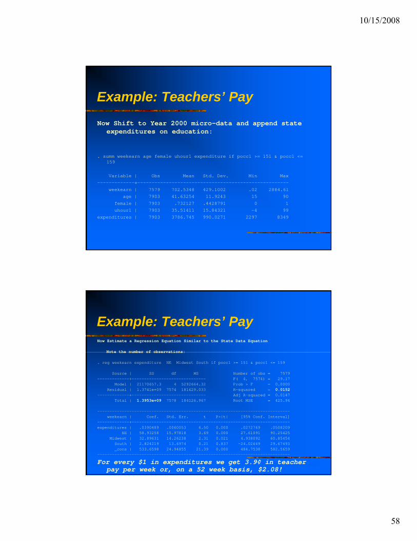
Now Shift to Year 2000 micro-data and append state expenditures on education:
. summ weekearn age female uhour1 expenditure if pocc1 >= 151 & pocc1 <= 159
Variable | Obs Mean Std. Dev. Min Max-------------+-----------------------------------------------------
k | 7579 702 5348 429 1002 02 2884 61weekearn | 7579 702.5348 429.1002 .02 2884.61age | 7903 41.63254 11.9243 15 90
female | 7903 .732127 .4428791 0 1uhour1 | 7903 35.51411 15.84321 -4 99
expenditures | 7903 3786.745 990.0271 2297 8349
Example: Teachers’ PayNow Estimate a Regression Equation Similar to the State Data Equation
Note the number of observations:Note the number of observations:
. reg weekearn expenditure NE Midwest South if pocc1 >= 151 & pocc1 <= 159
Source | SS df MS Number of obs = 7579-------------+------------------------------ F( 4, 7574) = 29.17
Model | 21170657.3 4 5292664.32 Prob > F = 0.0000Residual | 1.3741e+09 7574 181429.033 R-squared = 0.0152
-------------+------------------------------ Adj R-squared = 0.0147Total | 1.3953e+09 7578 184126.967 Root MSE = 425.94
------------------------------------------------------------------------------weekearn | Coef. Std. Err. t P>|t| [95% Conf. Interval]
-------------+----------------------------------------------------------------expenditures | .0390489 .0060053 6.50 0.000 .0272769 .0508209
NE | 58.93258 15.97818 3.69 0.000 27.61091 90.25425Midwest | 32.89631 14.26238 2.31 0.021 4.938092 60.85454
South | 2.824219 13.6974 0.21 0.837 -24.02649 29.67493_cons | 533.6598 24.94855 21.39 0.000 484.7538 582.5659
------------------------------------------------------------------------------
For every $1 in expenditures we get 3.9¢ in teacher pay per week or, on a 52 week basis, $2.08!

10/15/2008
59
Example: Teachers’ PayBuild a more suitable model and R-sq increases.
. reg weekearn expenditure female black NE Midwest South age coned if pocc1 >= 151 & pocc1 <= 159
Source | SS df MS Number of obs = 7479 -------------+------------------------------ F( 8, 7579) = 16.17
Model | 19477648.0 8 2434706.00 Prob > F = 0.0000Residual | 61297869.1 407 150609.015 R-squared = 0.2411
-------------+------------------------------ Adj R-squared = 0.2262Total | 80775517.1 415 194639.80 Root MSE = 388.08
------------------------------------------------------------------------------weekearn | Coef. Std. Err. t P>|t| [95% Conf. Interval]
-------------+----------------------------------------------------------------expenditures | .0636406 .0726116 0.88 0.381 -.0791 .2063811
female | -88.36832 43.00688 -2.05 0.041 -172.9117 -3.824972black | 72.28883 48.35753 1.49 0.136 -22.77287 167.3505
NE | -84.77944 116.1567 -0.73 0.466 -313.1213 143.5625Midwest | -38.8376 54.29961 -0.72 0.475 -145.5803 67.9051
South | -.8350449 48.33866 -0.02 0.986 -95.85964 94.18955age | 8.797438 1.653155 5.32 0.000 5.547649 12.04723
coned | 81.40359 11.48141 7.09 0.000 58.83332 103.9739_cons | -1089.701 300.7268 -3.62 0.000 -1680.873 -498.5296
------------------------------------------------------------------------------
Example: Teachers’ Pay
Why the difference in R-sq?Why the difference in R sq?Different levels of aggregation of data lead to different total variance.
Micro-data has much more variance than state average data (why might this be)?Times Series data often has r-sq of .98 or .99.A lt t R t th ltAs a result, we cannot use R-sq to compare the results across different data sets or types of regressions. It can be useful to compare specifications within a particular model.

10/15/2008
60
Correlation & R-Squared
R2 and ρ: What is the relationship?R and ρ: What is the relationship?ρ is the population value of the correlation, in the sample the symbol for correlation is r.If r is the correlation between X and Y, then R2, the goodness of fit measure of a regression equation is r2.N t th t thi ONLY h ld f bi i t l ti hiNote that this ONLY holds for bi-variate relationships.An example for the relationship between education expenditures and teacher pay:
Correlation & R-Squared: ExampleResults for: Teacher Expenditure.MTW
Correlations: pay, expenditures
Pearson correlation of pay and expenditures = 0.835P-Value = 0.000
Regression Analysis: pay versus expenditures
The regression equation ispay = 12129 + 3.31 expenditures
Predictor Coef SE Coef T PConstant 12129 1197 10.13 0.000expendit 3.3076 0.3117 10.61 0.000
S = 2325 R-Sq = 69.7% R-Sq(adj) = 69.1%
r2 = .8352 =.697225 = R2