Registration of Combined Range-Intensity

Scans: Initialization Through Verification

Eric R. Smith, Bradford J. King, Charles V. Stewart, Richard J. Radke

Rensselaer Polytechnic InstituteTroy, NY 12180

Abstract

This paper presents an automatic registration system for aligning combined range-intensity scan pairs. The overall approach is designed to handle several challengesincluding extensive structural changes, large viewpoint differences, repetitive struc-ture, illumination differences, and flat regions. The technique is split into threestages: initialization, refinement, and verification. During initialization, intensitykeypoints are backprojected into the scans and matched to form candidate trans-formations, each based on a single match. We explore methods of improving thisimage-based matching using the range data. For refinement, we extend the Dual-Bootstrap ICP algorithm for alignment of range data and introduce novel geometricconstraints formed by backprojected image-based edgel features. The verificationstage determines if a refined transformation is correct. We treat verification as aclassification problem based on accuracy, stability, and a novel boundary alignmentmeasure. Experiments with 14 scan pairs show both the overall effectiveness of thealgorithm and the importance of its component techniques.

Key words: range registration, iterative closest point, keypoint, decision criteria,physical changes

1 Introduction

This paper addresses the problem of automatically computing a three-dimensionalrigid transformation that aligns two range datasets, a problem that frequently

Email addresses: smithe4,kingb2,stewart@cs.rpi.edu,rjradke@ecse.rpi.edu (Eric R. Smith, Bradford J. King, Charles V. Stewart,Richard J. Radke).

Preprint submitted to Elsevier 10 August 2007

arises in three-dimensional (3D) modeling of large-scale environments and instructural change detection. We present a robust algorithm that can accuratelyestimate and verify this transformation even in the presence of widely-differingscanning viewpoints (leading to low overlap between scans) and substantialstructural changes in the environment between scans. Figure 1 illustrates twoexamples of challenging scans successfully registered using our framework.The first example shows the alignment of two scans of a building taken fromsubstantially different viewpoints, with trees occluding much of the commonstructure. The second example shows two scans of a parking lot and a build-ing taken four hours apart, with different vehicles appearing between the twoscans. Later in the paper, we demonstrate the alignment of a scan taken insidea room with one taken through a doorway looking into the room, as well asan alignment of two scans of a building where most of the common structureis repetitive (Figure 9).

We assume a range scanner that has an associated, calibrated camera ac-quires the datasets, producing point measurements in 3D and essentially-simultaneous intensity images. Many current range scanners have this dataacquisition capability, and it can be added to older scanners. Our registrationframework effectively exploits the information available in the range data, theintensity images, and the relationship between the two. It requires neitherexternal measurements such as GPS coordinates nor manual intervention.

Our fully automatic approach to registration involves three distinct stages— initialization, estimation, and verification — exploiting the combination ofrange and intensity information at each stage. During initialization, intensitykeypoints and their associated SIFT descriptors [39] are extracted from theimages and backprojected onto the range data. A three-dimensional coordi-nate system is established for each keypoint using its backprojected intensitygradient direction and its locally computed range surface normal. Keypointsare then matched using their SIFT descriptors. We explore several techniquesthat use the range data to improve the success of matching intensity keypoints.

Since each keypoint has an associated 3D coordinate system, each match pro-vides an initial rigid transformation estimate. This eliminates the need fora RANSAC-style search for minimal subsets of matches in order to gener-ate transformation estimates. Instead, the keypoint matches are rank-orderedbased on a distinctiveness measure, and each is then tested using the estima-tion and refinement procedures. As we will show, this approach is particularlyeffective for some of the most challenging image pairs because they have veryfew correct keypoint matches.

During the estimation stage, initial estimates are refined using a robust formof the Iterative Closest Points (ICP) algorithm [6, 14], starting with pointstaken only from the region surrounding the match in the two scans. The re-

2

Fig. 1. Two example challenging pairs that our algorithm registers (DCC and MRCParking lot). The top and center of the left column show a pair of scans taken fromvastly different viewpoints, in which trees occlude much of the common structure.The top and center of the right column show two scans of a parking lot and buildingwhere all of the vehicles are different between the two scans. In both cases, as shownon the bottom, the algorithm automatically and accurately aligned the scans. Thespheres in the figures indicate the scanner’s location.

3

gion is gradually expanded to eventually cover the overlap between the datasets. Region growth is controlled by the uncertainty in the parameter estimategenerated by ICP, with more certain estimates leading to faster growth. Thebasic structure is adapted from the Dual-Bootstrap algorithm previously pro-posed for 2D image registration [63,69], but incorporates several innovations torobustly solve the 3D rigid registration problem. For example, ICP correspon-dences are generated between range points and also between backprojectedintensity features. The latter produce constraints tangential to the range sur-faces, complementing the surface normal distance constraints generated fromthe range data. As we show experimentally, the growth and refinement pro-cedure nearly always converges to an accurate alignment given a reasonablyaccurate initial keypoint match. This shows further why a RANSAC-stylesearch is unnecessary.

The final part of the algorithm is a verification test to decide whether a refinedtransformation estimate is correct. This test uses a simple, yet effective, linearclassifier to combine measurements of alignment accuracy for both image andrange features, a measure of the stability of the estimate, and a measure ofthe consistency in the position of range boundaries. These measures, espe-cially the boundary measure, are more sophisticated than have been used inthe past [32], but are necessary for effective decisions when the scans involvephysical changes, simple geometries, and repetitive structures. Moreover, theireffectiveness enables a simple, greedy method of processing the rank-orderedinitial keypoint matches. That is, the matches are tested one-by-one; as soonas a candidate estimate passes the verification test, the result is accepted asa “correct” alignment. If all of the top M matches are rejected, the algorithmstops and reports that the scans cannot be aligned.

The overall algorithm is summarized in Figure 2 and described in detail in theremainder of the paper. Section 2 outlines related research. Section 3 discussesthe range/image data and the preprocessing of this data. Section 4 presentsthe initialization technique based on detection and matching of augmentedkeypoints. Section 5 describes the region-growing refinement algorithm basedon both range correspondences and backprojected intensity correspondences.Section 6 formulates the verification criterion. The overall effectiveness of thealgorithm, together with a detailed analysis of the individual components, ispresented in Section 7. Section 8 discusses the results, summarizes our contri-butions, and concludes the paper.

2 Related Work

The problem we address is a variation on the range scan registration problemthat has been studied extensively over the past several decades [12, 55, 56],

4

with solutions used in contexts as diverse as object modeling [4, 7], the studyof architecture [1], digitization of cultural artifacts [5, 38], and industrial in-spection [48]. Work on range image registration can be roughly divided intotechniques for (1) initial registration or coarse alignment of a pair of scans,(2) fine registration of scan pairs, and (3) simultaneous registration of mul-tiple scans given the results of pairwise scan registration. While the latteris an important problem [4, 7, 32, 51, 59], we focus here on the problems ofinitialization and refinement for a scan pair, while adding the substantial-but-not-well-studied issue of determining when the scans are well-aligned or caneven be aligned at all.

A wide variety of techniques have been proposed for initial registration ofrange scans. All are based on extracting and matching summary descriptionsof the scans. Some methods use extraction and matching of distinctive loca-tions, such as points of high curvature [15] or other extremal locations [66].Other feature-based methods have been developed for specific contexts, forexample exploiting the presence of windows and building corners in the regis-tration of architectural scans [13,61]. A second set of approaches, mostly usedfor aligning scans of single, smooth objects, includes methods that extractand match summary descriptions over small regions of the data. These in-clude point signatures [16], “splashes” [62] and the more recent integral pointdescriptors [23]. A third set is comprised of methods that summarize largerregions or even the entire scan as the basis for registration and 3D objectrecognition. This includes work on extended Gaussian images (EGIs) [31] andspherical attribute images (SAIs) [29], where shapes are described using amapping of a scan onto a sphere based on estimated surface normals. Thiswork has mostly been superseded by spin images [33, 35], extensions of theshape-context work [2] to 3D [21], and tensor-based methods [43]. Recently,Makadia et al. [40] resurrected the use of EGIs by reducing the EGI to a“constellation” of peak locations on the Gaussian sphere and matching theseconstellations between scans. This matching leads to the generation of severalrelative pose hypotheses between scans, each of which is then tested. Thistheme of hypothesis generation and testing is echoed in our approach.

When calibrated intensity images are available in addition to range scans,intensity features may be combined with range information to develop differentinitialization methods. One approach is to augment large region descriptorssuch as spin images with intensity data, producing a hybrid descriptor [11]. Amore common approach is to build on the rapid progress that has been maderecently in the matching of intensity keypoints between images taken over largechanges in viewpoint [45, 46]. Proposed keypoint detection techniques havebeen based on the Laplacian-of-Gaussian operator [39], information theory[36], Harris corners [44], and intensity region stability measures [41]. Followingdetection, summary descriptions of keypoints are constructed as the basis formatching. While a number of methods have been proposed [2, 20, 25, 39], the

5

SIFT descriptor [39], a spatial histogram of intensity gradients, has proved themost effective [45]. Several authors have proposed combinations of keypointdescriptor methods with range data for the initialization problem. Roth [53]used a combinatorial search to match keypoints that have been backprojectedinto 3D, but did not exploit the intensity information in the matching process.Wyngaerd and Van Gool [67] extracted and matched combined intensity andrange feature vectors, computed at the intersection of a sphere with the rangesurface. Bendels et al. [3] matched 2D SIFT features, backprojected them ontothe range data, and then used RANSAC on these points in 3D to identify aninitial rigid transformation and filter incorrect matches. This does not exploit3D information during the computation of the SIFT descriptor, as has beenshown in [57] as well as our own earlier work [37]. In particular, Seo et al. [57]used 3D geometry to eliminate keypoints in non-planar regions and to rectifySIFT regions prior to computing the descriptor. We explore similar techniqueshere and also analyze in detail the effectiveness of this method.

We now turn to the refinement stage of registering a pair of range scans. In theliterature, refinement usually depends on application of the well-known itera-tive closest point (ICP) algorithm [6,14,42]. ICP starts from an initial trans-formation estimate, and uses this to map points from one scan (the “moving”scan) onto the second scan (the “fixed” scan) in order to establish temporarycorrespondences between points in the two scans. These correspondences arethen used to refine the estimate. The process iterates until a convergence cri-terion is met. The simplest and most common basis for establishing correspon-dence is the original idea of minimizing geometric distance between points, al-though a variety of shape properties has been exploited as well [58]. Distancemetrics used in the estimation step of ICP have focused on the Euclideandistance and point-to-plane distance (“normal distance”) measures, but morerecently, quadratic approximations [47] have been proposed. Efficient varia-tions of ICP have been studied extensively [55]. Earlier work [17, 70] studiedrobustness to missing components of scans due to differences in viewpoints.The matching and refinement loops of ICP were cast into a Expectation Max-imization (EM) framework in [26]. Genetic algorithms have been applied toimprove the domain of convergence of ICP [10]. Convergence properties ofICP were studied recently by Pottmann et al. [50]. This work clearly showsthe advantage of using normal distances instead of Euclidean distances, andsuggests even faster convergence with higher-order distance approximations.A version of normal-distance ICP that is robust to mismatches and missingstructures is at the core of our refinement algorithm.

Several researchers have combined intensity information with ICP. In one ap-proach, color is treated as an additional geometric attribute to be combinedwith position in the determination of correspondences in ICP matching [19,34].An alternative approach uses intensity and other geometric attributes to filterclosest point matches [24, 49]. Projection-based methods have been proposed

6

as well, using image-based optical flow for matching [68] and, more recently,using color and depth differences in 2D coordinate systems to drive 3D regis-tration [52]. Overall, two difficulties arise when combining range and intensityinformation to drive ICP that are especially significant in our particular prob-lem domain: (1) intensity/color information and range data have differentmetric properties, and (2) intensities can change substantially between scans.We address both of these problems below through a novel technique that usesgeometric constraints derived from matching backprojected image features.

The final concern is the problem of determining if two scans are actuallywell-aligned. This issue has received much less attention than initializationand refinement, in large part because of the limited domain in which fullyautomatic registration has been applied. Silva, Bellon and Boyer proposed an“interpenetration measure” that checks the fine alignment of two surfaces [60].The most extensive work is that of Huber and Hebert [32] whose algorithmtests both alignment accuracy and the fraction of mismatches that do notviolate visibility constraints. In our context, visibility constraints must becarefully defined to accommodate for the possibility of changes between scans.Our approach does not exploit visibility directly, but instead looks at measuresof accuracy, stability, and the alignment of visible depth discontinuities. Ourdecision measures substantially extend our earlier work both for range imageregistration [37] and intensity image registration [69]. Finally, in registrationand mosaic construction based on keypoint matching, combinatorial analysisof keypoint match count provides a probabilistic measure of correctness [8].Such an approach does not work here due to the low number of correct keypointmatches in difficult scan pairs.

3 Preprocessing and Feature Extraction

This section discusses Steps 1 and 2 of our algorithm (Fig. 2), the preprocess-ing of the range data and the intensity images, including backprojection ofintensity features onto surfaces approximated from the range data.

We denote the set of points associated with a scan as P , and the individualpoint locations as Pi ∈ P . As mentioned above, we assume a range scan-ner that has an associated, calibrated camera acquires the datasets. Since allpoints in a scan are acquired from a single viewpoint, the points can be easilymapped into a spherical coordinate system and binned in two dimensions us-ing the spherical angles. One use of this binning structure is to find the nearestscan point Pi to any backprojected image point, which is straightforward be-cause the image and range scanner viewpoints nearly coincide. A second useis to accelerate matching through computation of approximate closest pointsas in [55].

7

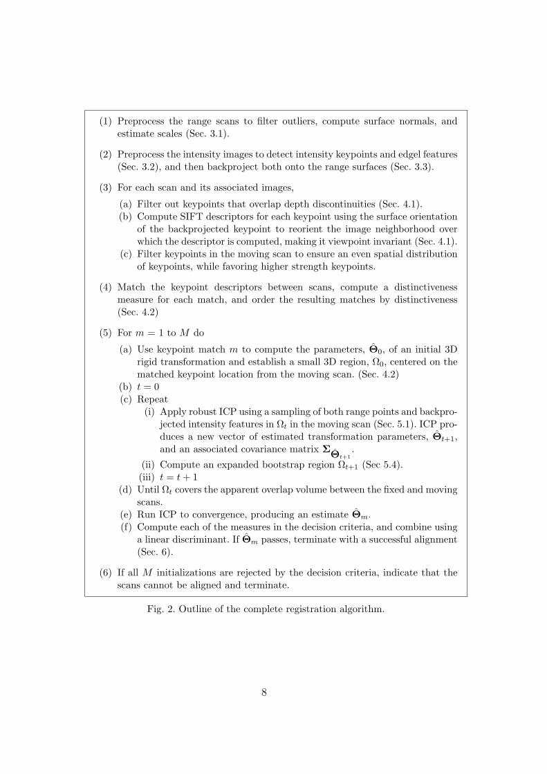
(1) Preprocess the range scans to filter outliers, compute surface normals, andestimate scales (Sec. 3.1).

(2) Preprocess the intensity images to detect intensity keypoints and edgel features(Sec. 3.2), and then backproject both onto the range surfaces (Sec. 3.3).

(3) For each scan and its associated images,

(a) Filter out keypoints that overlap depth discontinuities (Sec. 4.1).(b) Compute SIFT descriptors for each keypoint using the surface orientation

of the backprojected keypoint to reorient the image neighborhood overwhich the descriptor is computed, making it viewpoint invariant (Sec. 4.1).

(c) Filter keypoints in the moving scan to ensure an even spatial distributionof keypoints, while favoring higher strength keypoints.

(4) Match the keypoint descriptors between scans, compute a distinctivenessmeasure for each match, and order the resulting matches by distinctiveness(Sec. 4.2)

(5) For m = 1 to M do

(a) Use keypoint match m to compute the parameters, Θ0, of an initial 3Drigid transformation and establish a small 3D region, Ω0, centered on thematched keypoint location from the moving scan. (Sec. 4.2)

(b) t = 0(c) Repeat

(i) Apply robust ICP using a sampling of both range points and backpro-jected intensity features in Ωt in the moving scan (Sec. 5.1). ICP pro-duces a new vector of estimated transformation parameters, Θt+1,and an associated covariance matrix Σ ˆΘt+1

.

(ii) Compute an expanded bootstrap region Ωt+1 (Sec 5.4).(iii) t = t + 1

(d) Until Ωt covers the apparent overlap volume between the fixed and movingscans.

(e) Run ICP to convergence, producing an estimate Θm.(f) Compute each of the measures in the decision criteria, and combine using

a linear discriminant. If Θm passes, terminate with a successful alignment(Sec. 6).

(6) If all M initializations are rejected by the decision criteria, indicate that thescans cannot be aligned and terminate.

Fig. 2. Outline of the complete registration algorithm.

8

3.1 Range Scan Preprocessing

The scan points in 3D are preprocessed to eliminate outliers, to estimate asurface normal, ηi, associated with each point, and to estimate the uncer-tainty in feature position along this normal in real units, represented as ascale (standard deviation) σi. The normal estimation algorithm uses a ro-bust least-squares approach applied over a small, adaptive neighborhood thatavoids rounding of sharp edges. The values of the scale estimates depend onboth the noise in the scanner (2-4 mm for our scanner) and the degree towhich the surface varies from planarity. The latter is particularly importantbecause the intersample spacing is relatively high (e.g. 2-5 cm) and surfacesin outdoor scenes can be quite rough. Thus, the estimated scale values tendto vary across the data set and can be as high as 1-2 cm. This consideration isimportant because even for perfectly-aligned scans, “correct” correspondencesmay be separated by up to half the sample spacing on the surface; there-fore, interpreting any measure of distance between corresponding points mustconsider this locally-estimated scale.

The final step in preprocessing the range scans is to locate non-trivial depthdiscontinuities. Adjacent discontinuity locations in the scan grid are linked toform chains; the very short chains and smaller discontinuities are discarded. Inoutdoor scans, these discarded points usually correspond to boundaries in treesor grass, which are unlikely to be stable in subsequent scans. The remainingboundaries are used in the verification tests, as discussed in Section 6.

3.2 Keypoint and Intensity Feature Detection

Next, keypoints are located in the intensity images. These will be used as thebasis for initialization of the transformation estimate. We also locate intensityfeatures, which will be used in ICP refinement of the transformation estimate.

We define keypoints as scale-space peak locations in the magnitude of theLaplacian-of-Gaussian operator, as in the well-known SIFT algorithm [39].We use techniques similar to those in [9] to ensure widespread feature distri-butions. In particular, the minimum spacing between keypoints is set to belinearly proportional to the product of the field of view angles of the scanner.This ensures a sufficient number of keypoints for small fields of view withoutgenerating an overly large number of keypoints for larger fields of view.

At the end of the keypoint computation, each keypoint has an associatedlocation uj, gradient direction gj and detection scale sj, all measured in imagecoordinates.

9

The intensity features are sampled edge elements (edgels) — image locationshaving a significant peak in the gradient magnitude along the gradient direc-tion. The detection technique is similar to the edge detection method proposedin [27]. Adaptive thresholding is used to ensure a widespread distribution offeatures. Just as with keypoints, each feature has an associated normal direc-tion nj, location uj, measured to subpixel accuracy along nj, and detectionscale sj.

3.3 Backprojection

Pj

uj

gj

Uj

scanner / camera

image plane

scene patch

Fig. 3. Keypoints and associated image gradients are backprojected to form a 3Dcoordinate frame around each backprojected point.

Both keypoints and features are backprojected into 3D as illustrated in Fig-ure 3. The line of sight associated with image point uj is found and the closestscan point Pj is found to this line of sight. The intersection of the line of sightwith the plane defined by Pj and its normal ηj determines the backprojectedlocation, Uj. The backprojection of gj is the unique direction vector, γj, thatis normal to ηj and projects into the image at uj parallel to gj. A 3D coordi-nate system is established at Uj by making γj the x axis, ηj the z axis andηj × γj the y axis. Finally a scale Sj is computed from sj by backprojectingthe point uj +sjgj onto the plane and computing the distance of the resultingpoint to Uj. This is the physical analog to the detection scale in the image.

10

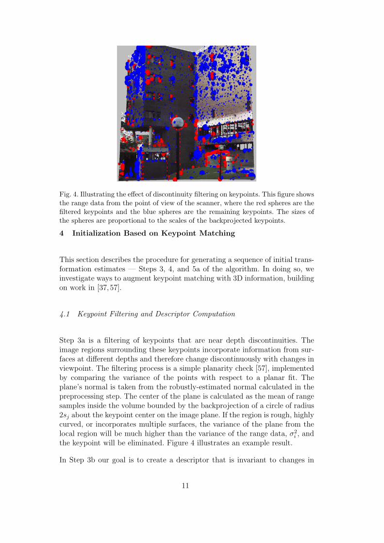
Fig. 4. Illustrating the effect of discontinuity filtering on keypoints. This figure showsthe range data from the point of view of the scanner, where the red spheres are thefiltered keypoints and the blue spheres are the remaining keypoints. The sizes ofthe spheres are proportional to the scales of the backprojected keypoints.

4 Initialization Based on Keypoint Matching

This section describes the procedure for generating a sequence of initial trans-formation estimates — Steps 3, 4, and 5a of the algorithm. In doing so, weinvestigate ways to augment keypoint matching with 3D information, buildingon work in [37,57].

4.1 Keypoint Filtering and Descriptor Computation

Step 3a is a filtering of keypoints that are near depth discontinuities. Theimage regions surrounding these keypoints incorporate information from sur-faces at different depths and therefore change discontinuously with changes inviewpoint. The filtering process is a simple planarity check [57], implementedby comparing the variance of the points with respect to a planar fit. Theplane’s normal is taken from the robustly-estimated normal calculated in thepreprocessing step. The center of the plane is calculated as the mean of rangesamples inside the volume bounded by the backprojection of a circle of radius2sj about the keypoint center on the image plane. If the region is rough, highlycurved, or incorporates multiple surfaces, the variance of the plane from thelocal region will be much higher than the variance of the range data, σ2

i , andthe keypoint will be eliminated. Figure 4 illustrates an example result.

In Step 3b our goal is to create a descriptor that is invariant to changes in

11

Fig. 5. Illustrating the computation of the augmented keypoint descriptor. The affinemapping from the surface tangent plane to the image plane determines a mappingbetween a square grid on the surface and an affine grid in the image. On the leftthe augmented keypoint descriptor is shown on the range plane it is computed on –the affine approximation is visible here since the descriptor region is not a perfectsquare. The right image shows the descriptor region projected into the image plane.

viewpoint. Our strategy is to compute a SIFT descriptor [39] using the planarsurface centered at the backprojected keypoint (see Sec. 3.3) to create an affinere-mapping of the image region. Algorithms that work with intensity imagesalone use the image data itself to infer such an affine mapping [46].

Recall that the SIFT descriptor is formed as a 4 × 4 spatial grid of orien-tation histograms, with 8 orientation bins per histogram. Concatenating thehistograms and normalizing gives the 128-component descriptor vector. In ourtechnique, the SIFT 4× 4 square grid is aligned with the x and y axes of thekeypoint’s backprojected coordinate system and the size of the grid is deter-mined by the backprojected detection scale. Using an affine approximation tothe mapping between this tangent plane and the image plane, the boundariesof this grid are mapped into the image plane, and the image locations andgradients falling within these boundaries are mapped back onto the surface.The backprojected locations are used to assign the points to one of the 4× 4SIFT grids and the affine-mapped gradient vectors are entered into the 8-bin orientation histogram associated with each grid block. After all gradientshave been entered into the histograms, each histogram entry is divided by theamount of interpolated weight that its grid block received. The 128-componentdescriptor is then extracted, and it is normalized in the same way as in [39].Modulo sampling and other imaging artifacts, the resulting descriptor shouldbe invariant to image scaling and to rotation and translation in 3D. This is asimilar approach to Seo et al [57]; however, we use only affine approximationand do not resample the actual intensities. The process is illustrated in Figure5.

12

4.2 Matching and Initialization

The keypoints extracted from two scans are matched based on the SIFT de-scriptors of the keypoints as in [39]. The backprojected scales of the keypointsare approximate physical scales and therefore, in theory, should be invariantto the position of the scanner. A keypoint match is only allowed if the ratio ofthe larger to the smaller scale is less than a constant. (This type of comparisonis possible because the constraints are based on back-projected and thereforephysical scale measurements.) We have experimentally determined an effectivevalue of this constant to be 2.0, reflecting the uncertainty in the estimates ofscale due to sampling and the lack of affine correction of the scale estimate.

For each keypoint from one scan, among the matches allowed by the scaleratio test, the two keypoints whose descriptor vectors are closest in Euclideannorm are located. We define the distinctiveness measure of the best match asthe ratio of the best to the second best descriptor distance [39].

The keypoint matches are ordered by increasing value of the distinctivenessmeasure and tested in this order in the next step. For each match tested,simply computing the transformation between the backprojected coordinatesystems of the two keypoints generates an initial 3D rigid transformation.The initial region, Ω0, starts as a cube aligned with the axes of the movingscanner’s coordinate system, with side length 8 times the maximum of thepoint spacing and the backprojected pixel spacing on the surface. This initialregion is expanded if necessary to contain at least 100 range points.

5 Refinement

The goal of refinement is to substantially improve the initial keypoint-basedalignment between scans. This is done iteratively by alternating steps of (a) re-estimating the transformation using only matches for points in the bootstrapregion Ωt and (b) expanding the bootstrap region. Several iterations of refine-ment are illustrated in Fig. 6. Aside from this region growth procedure, themost important novel contribution in this section is the combination of rangescan correspondences and back-projected intensity feature correspondences inestimating the rigid transformation parameters.

13

Fig. 6. Several iterations of ICP estimation and region growth of a relatively easypair called “VCC North”. The colored regions represent the area inside the currentbootstrap region, Ωt. The first frame shows the initial alignment of the scans andthe initial region. Subsequent frames show the alignment and the region followingiterations 1, 2, 5, 8, and 14 respectively. The correction of the strong initial mis-alignment can be clearly seen. Regions that are solidly one color or the other wereonly seen from the viewpoint of one scan.

5.1 Robust ICP

The core idea of ICP is well known. An initial transformation estimate is usedto map points from the moving scan to the fixed scan. For each mapped point,the closest point in the fixed scan is located and these two points are usedto form a temporary correspondence. The set of all such correspondences isused to re-estimate the parameters of the transformation. The whole processthen iterates until some convergence criterion is met. In our refinement step,we do not wait for ICP to converge for each bootstrap region Ωt, but insteadstop and expand the region after two ICP iterations. After region growth hasconverged ICP continues to run until convergence.

Let Θ be the current parameter estimate and, for moving point Pi, let

P′i = T(Pi; Θ).

be the mapped point. Next, let Qj be the closest point, in Euclidean distance,to P′

i. This forms the correspondence (Pi,Qj). Let ηj be the precomputed(unit) surface normal at Qj. The objective function for estimating the param-

14

eters from this set of correspondences is

F (Θ) =∑

(Pi,Qj)

ρ([T(Pi; Θ)−Qj]>ηj/σi,j), (1)

where[T(Pi; Θ)−Qj]

>ηj (2)

is the “normal distance” — the distance from T(Pi; Θ) to the plane throughQj with normal ηj — and ρ is a robust loss function. We use the Cauchy ρfunction,

ρ(u) =C2

2log

(1 +

u2

C2

), (3)

with C = 2.5 (consistent with typical values from the statistics literature [30]).Finally, σ2

i,j is the variance in the normal distance alignment error of the match.Estimation of σ2

i,j is discussed in detail below.

Minimization of F (Θ) to produce the next estimate Θ is accomplished usingiteratively reweighted least squares (IRLS) [64], with weight function

wi,j =1

σ2i,j

ρ′(ui,j)

ui,j

=1

σ2i,j(1 + u2/C2)

(4)

where ui,j = [T(Pi; Θ)−Qj]>ηj/σi,j, and weighted least-squares formulation

Fw(Θ) =∑

(Pi,Qj)

wi,j[(T(Pi; Θ)−Qj)>ηj]

2 (5)

In each iteration of IRLS, the update to the parameter estimate is achievedusing the small-angle approximation to the rotation matrix. Since the incre-mental changes to the parameters tend to be small, this approximation workswell. At the end of these two iterations the covariance matrix, ΣΘ, of the trans-formation parameters is estimated from the inverse Hessian of (5). See [22,65]for more details.

5.2 Backprojected Intensity Constraints

The algorithm description thus far has not included constraints from matchingbackprojected intensity features. A novel step in our work is to use these asgeometric constraints in the same way as correspondences from range pointmatching. Our goal is to create constraints on the 3D rigid transformation thatcomplement the constraints from range matches. Since the latter are based ondistances normal to surfaces, we design the intensity constraints to operatetangentially to surfaces (Fig. 7). The importance of this is most easily seen inthe extreme case of aligning scans of a single, patterned, planar surface: range

15

correspondences would only determine three degrees of freedom (DoF) of thetransformation, leaving two translational and one rotational DoF in the plane.The intensity feature correspondences are designed to determine these threeDoF.

Range Constraints Intensity Constraints Combined Constraints

Fig. 7. Illustrating the complementary role of constraints from matching range pointsand from matching backprojected intensity features. Range matches provide con-straints normal to the surface, while backprojected intensity feature matches provideconstraints in the tangent plane of the surface. The top row shows the features pro-viding constraints. The bottom row shows constraints placed on a rigid transformby each group of features. Circles represent rotational degrees of freedom and linesrepresent translational degrees of freedom. Highlighted circles and lines indicatethose that are constrained.

As mentioned earlier, within the 2D image, each intensity feature has a loca-tion and a normal. These are backprojected onto the estimated surface in 3D,giving a location Uj, and direction γj. The latter is in the tangent plane ofthe surface. When this backprojected feature is correctly matched to a back-projected feature Vi from the moving scan and the transformation correctlyaligns the points, then (ignoring noise) we should have

[T(Vi; Θ)−Uj]>γj = 0. (6)

Since this has the same form as the normal distance constraint (2), we canmatch backprojected image features and use them to constrain the estimateof transformation parameters in the same manner as range correspondencesand their constraints. This makes implementation straightforward.

There are several important details to making this approach succeed. The

16

first and the most important issue is estimating the variance σ2i,j of the align-

ment error for both types of correspondences. This is used both to separateinliers from outliers and to assign relative strength to the two types of con-straints — larger variances on one type of constraint lead to lower overallweight (4), even for inliers, and therefore less influence on the transformationparameter estimate. Estimation of variance is discussed in detail in the nextsection. Second, when sampling points in the current moving scan region Ωt

to form matches and thereby constraints on the transformation, the algorithmattempts to choose the same number of each type of feature. We rely on thecomputation of the variances and the resulting robust weights (4) to balancethe relative influence of the two types of constraints. Finally, for intensityfeature matches, we use the Beaton-Tukey biweight function

ρ(u) =

(1− u2/B2)3 |u| < B

0 |u| ≥ B, (7)

as in [69], in place of the Cauchy loss function (3), with B = 4.5 (consistentwith parameters developed in the statistics literature [30]). The Beaton-Tukeyfunction more aggressively downweights potential outliers, which is more ap-propriate for image-based constraints where there tend to be more outliers —mostly due to viewpoint and illumination changes — and the alignment errorsof these outliers tends to be only marginally higher than that of the inliers.

5.3 Correspondence Variances

When estimating the rigid transformation parameters for a fixed set of matches,the variance in the alignment error, through its effect on the weight function(4), is used to eliminate the influence of outlier matches and to balance theinfluence of constraints from range point correspondences and from backpro-jected image feature correspondences. This prominent role of the variancemarks a different approach to robustness than prior work on range registra-tion [17,70], but it is consistent with traditional robust estimation methods [64]as well as our own prior work on registration [69]. The particular challengefaced here is that the variance must be treated as both unknown and varyingfrom point to point. The latter follows from two observations: (1) as discussedin Sec. 3.1, due to intersample spacing, surface roughness and surface curva-ture, the variance in the locally-estimated planar surface approximation tendsto change substantially from range point to range point, and (2) the variancein the positions of backprojected intensity features tends to increase with dis-tance from the scanner.

In order to make the problem of estimating the alignment error variancestractable, we make two simplifying assumptions. First, the alignment error

17

variance is assumed to be proportional to the sum of the variances of the pointpositions along their normal direction. Thus, if σ2

i and σ2j are the variances of

the moving and fixed points, Pi and Qj respectively, then the variance in thenormal distance alignment error, [T(Pi; Θ)−Qj]

>ηj, is modeled as

σ2i,j = k2

c (σ2i + σ2

j ), (8)

with kc as yet unknown. This assumption (which also depends on the pointposition errors in the two scans being independent of each other and primarilyalong the surface normal directions) is reasonably accurate at convergence,when the surfaces’ normals are aligned and the primary factor in the remainingerror is due to point position errors rather than uncertainty in the parameterestimate. Moreover, since the parameter estimate tends to be quite accuratewithin the bootstrap region throughout the computation, the approximationholds during all iterations. Indeed, we have found experimentally that theestimated value of kc stays quite close to 1.0 for range feature correspondences.

The second assumption is that the error in the true position of the image fea-tures in the image coordinate systems is proportional to the image smoothingscale at which they are detected. This ignores a number of properties of theimaging process and the imaged surfaces; focusing only on the well-knowneffect that smoothing has on edge-position uncertainty. We have found thisassumption to be a reasonable first approximation both in past work [69]and in the algorithm described here. Given this assumption, the variance ofa backprojected image feature at location Ui is k2

eS2i along the backprojected

direction γi (which is in the surface tangent plane), where Si is the backpro-jection of the smoothing scale for image feature i. Combining this with (8)yields the variance for correspondences between backprojected image featuresas

σ2i,j = k2

ck2e(S2

i + S2j ) = k′c

2(S2

i + S2j ). (9)

In the latter, we have combined the two unknowns into a single value k′c.Thus, we have the same form for the variance in the normal-distance alignmenterror for both range point correspondences and backprojected intensity featurecorrespondences.

The Appendix describes how the scaling factor kc is estimated from a givenset of correspondences. Estimation of k′c is identical, and we never explicitlyestimate ke.

5.4 Region Growth

The region growth technique is a simple extension of the region growth tech-nique for two-dimensional images used in the Dual-Bootstrap algorithm [63,69]. As mentioned earlier, the region is an axis-aligned rectangular solid in

18

3D, and all computation is done in a coordinate system centered on this solid.Growth occurs by considering the location Y in the center of each face of thesolid, and computing the transfer error covariance [28, Ch. 4] of the mappingof this point. If the Jacobian of the mapping function is J = ∂T/∂Y, thetransfer error covariance matrix of the mapped point Y′ = T(Y; Θ) is

ΣY′ = JΣθJ>. (10)

Here, the rotation component of the transformation is parameterized usingthe small angle approximation, making Σθ a 6×6 matrix, the Jacobian 3×6,and the resulting transfer error covariance, ΣY′ 3 × 3. The latter covarianceis projected onto the outward face normal of the rotated Ωt at Y′. Growthis inversely proportional to the resulting scalar variance value. Each side isallowed to expand by up to 50% of its distance from the center, indicatingthat the solid can at most double in size in each dimension. This only occurswhen there is a great deal of confidence in the estimate, and growth is typicallyslower earlier in the computation.

5.5 Iterations and Convergence

Since normal-distance ICP does not provably converge, neither does our over-all refinement algorithm. However, we have not encountered a problem thatdoes not converge in practice. Our criterion for region growth convergenceis that Ωt has expanded sufficiently to cover the region of overlap (as com-puted from the estimated transformation) between the two scans. Our crite-rion for ICP convergence is that the mapping of points on the region boundarydoes not change substantially between ICP iterations. Region growth typicallyconverges in about 10 iterations, and ICP converges almost immediately af-terward. Since many of the earlier iterations occur with significantly fewercorrespondences, overall convergence is quite fast (see Section 7.4).

6 Decision Criteria

After the refinement procedure converges, the algorithm checks the result todetermine if the alignment is sufficiently accurate and reliable to be consideredcorrect. The challenge in doing so is handling potential structural/illuminationchanges as well as low scan overlap. Thus, measures such as Huber’s visibilitytest [32], which assumes no changes between the scans, cannot be used. Ourtest incorporates seven measures: accurate alignment of both image featureand range correspondences; accurate alignment of normal directions for bothimage feature and range correspondences; stability of the transformation es-timate; and two novel boundary alignment measures. These are all combined

19

using a linear classifier to determine whether the registration is correct orincorrect.

6.1 Positional Accuracy

Accuracy is the most natural measure. We use the normal-distance alignmenterror of the correspondences from the last iteration of refinement after regiongrowth has converged. For range scan correspondences this is

PAR =

∑(Pi,Qj)

wi,j[(T(Pi; Θ)−Qj)>ηj]

2k2c (σ2

i + σ2j )/

∑(Pi,Qj)

wi,j

1/2

. (11)

An identical measure, denoted by PAI , is used for image feature correspon-dences.

6.2 Angular Accuracy

The angular accuracy measure ensures that the feature directions — rangesurface normals and backprojected feature normals — are well-aligned, com-plementing the positional accuracy measure. This is most effective for testingimage feature correspondences, since their normal directions vary much morequickly than the normals of smooth surfaces. For any correspondence (Pi,Qj)from the final ICP iteration, let wi,j be the final weight, let η′i be the mappingof Pi’s normal direction into the fixed image, and let αi,j be the angle betweenη′i and ηj. Then the angular accuracy measure is

AAR =∑

(Pi,Qj)

wi,j|αi,j| /∑

(Pi,Qj)

wi,j. (12)

The analogous measure AAI is computed for image feature correspondences,except that the angles are mapped into [0 . . . π/2) prior to computing AAI toaccount for the possibility of contrast reversals [69].

6.3 Stability

Incorrect transformations tend to be less stable than correct ones, especiallywhen low inter-scan overlaps are allowed. Stability is measured using the trans-fer error covariance computation, which was already used for region growthin a previous stage (Sec. 5.4). A bounding box is placed in the moving scan

20

around the points that have correspondences with non-zero weight. The traceof the transfer error covariance ΣY′

i(Eqn. 10) is then maximized over this box,

with the result being the stability measure, ST. The trace is used because itcaptures the uncertainty in any direction.

6.4 Boundary Alignment Check

While the four accuracy measures and the stability measure are strong indi-cators of correctness, they still produce false positives, most notably in scenesinvolving repetitive structure. A common example is aligning two scans of theface of a building that has regularly-spaced windows. An estimated alignmentthat produces a shift in the scans by the inter-window spacing looks very sim-ilar to a correct alignment. If we could assume that there were no changes inthe scene between the two scans, then this misalignment could be caught byHuber’s visibility test [32]. Since we are considering the potential for structuralscene changes (along with small overlap and substantial viewpoint changes),a more sophisticated test is needed.

The test we propose is based on surface boundaries, detected as part of thepreprocessing step (3.1). We do not take the natural step of establishing cor-respondences between boundary points in the two scans, in large part becauseviewpoint differences may cause a boundary (a depth discontinuity) in onescan to be missed in the other. Instead, each sampled boundary point, j, fromthe moving scan is tested as follows (see Figure 8). Two boxes are formed: Bi

on the surface interior, where samples occur, and Be on the surface exterior,where no points are measured. If the two scans are properly aligned, thenwhen Bi is mapped into the fixed scan, it should contain fixed-scan points,whereas when Be is mapped into the fixed scan, it should be empty. Whenboth mapped boxes contain fixed-scan points, this is evidence of a misalign-ment, whereas when both are empty, this is evidence of either a misalignmentor a structural change. Since there is one box per boundary point and thespacing between boundary points is at the sampling resolution of the scanner,upwards of several thousand boundary boxes are formed per scan, allowing foran aggregate computation of our boundary measures and tolerance to changesand transient objects that may affect the measure in a small number of boxes.

Here are details on the formation of surface interior box Bi and exterior boxBe for one boundary point. The axes of Bi are the estimated surface normalat the boundary, the boundary chain direction (lies on the estimated surface),and a third axis perpendicular to the other two. This construction ensures theinclusion of sample points. For Be, one axis is parallel to the edge tangent,one is parallel to the scanner’s line of sight at the boundary, and the thirdis perpendicular to the other two. By orienting Be in this way, it should be

21

empty in the fixed scan regardless of the type of boundary — a true surfacediscontinuity, a crease edge, or a location where the surface is tangent to thescanner’s line of sight. The boxes are both wide enough (in the tangentialdirections) to accommodate sample spacing in the fixed scan and tall enoughto account for noise (8).

Three different boundary point counts are formed: N is the total number ofboundary points tested; Ni is the number of boundary points, j, such thatj has at least a minimum number of fixed points in its interior box Bi aftermapping into the fixed scan; Nie is the number of boundary points, j, suchthat (a) j is counted in Ni and (b) j’s exterior box Be is also (nearly) empty inthe fixed scan. 1 In other words, boundary points counted in Nie have occupiedinterior boxes and empty exterior boxes in the fixed scan. The three countsare used to form two boundary measures for a given alignment: BT1 = Nie/Ni

and BT2 = Nie/N . Ideally, both scores will be near 1, but when there aresubstantial structural changes between scans, BT2 may be low. On the otherhand, BT1 cannot be used alone because severe misalignments can cause it tobe high and BT2 to be very low. We let the linear classifier determine the trade-off between these measures (and the other decision measures) automatically.

FixedFixed

Moving

OcclusionBoundary

Fixed

Occludedwithout

Boundary

Moving Moving

ViolationNo Violation

Bi

Be

Bi

Be

Bi

Be

Fig. 8. Construction and use of the boundary test boxes. In the moving scan (topleft), Bi, the interior box, is aligned with and centered on the surface near to but notoverlapping the boundary, and Be, the exterior box, is aligned with the line-of-sightdirection and centered at the depth of the boundary point. When these boxes aremapped into the fixed scan (top right), Bi should contain surface points and Be

should be empty, even when the location corresponding to the boundary point isalong an edge and the surfaces on both sides of the edge are visible. The bottom leftand right images illustrate cases with no violation and violation of the boundaryconstraints, respectively.

1 Be will not always be completely empty, even for correct boundaries, because ofboundary curvature and because scanners tend to produce points that interpolatebetween foreground and background surfaces at discontinuities.

22

6.5 Classification

For each rigid transformation parameter estimate produced by the refinementprocedure, seven measures are computed from the parameters, the parametercovariance matrix, the matches and the boundary points — the two positionalaccuracy measures, PAR and PAI , the two orientation accuracy measures, AAR

and AAI , the stability measure, ST, and the two boundary measures BT1 andBT2. These are each computed with neither re-matching nor re-estimation.The values are input into a linear classifier, which outputs a binary accept /reject decision. This classifier is trained using the Ho-Kashyap algorithm [18]on the data described below.

7 Experimental Evaluation

Our experiments evaluate both the overall effectiveness of the algorithm andthe importance of the individual algorithm components. We collected a set of14 test scan pairs exhibiting many challenging aspects of range scan registra-tion, including three with substantial illumination differences, four with largechanges in viewpoint, four with changes in structure, two having low overlap,one taken of an entirely planar scene, and three dominated by repetitive struc-tures. Only three of the scan pairs, all taken outdoors, would be considered“easy”. Two “hard” pairs and their resulting alignments are shown in Fig. 1,and four other “hard” pairs are shown in Fig. 9. The remaining eight pairs areshown in Fig. 10. The abbreviations indicated in the figures are used in theresult tables below. Six of the 14 pairs were used for tuning the initializationand refinement parameters. Six pairs are also used for the training involvedwith the decision criteria (Section 7.3). There were no substantial differencesin the results for the training and test sets, so the results are lumped togetherfor the sake of brevity.

The range scans were collected using a Leica HDS 3000 scanner. The scans inour experiments were typically acquired at 2-5 cm linear sample spacing onthe surfaces. The RMS error of the measured points is 2-4mm, independent ofdepth, on matte planar surfaces. The scanner acquires intensity images usinga fixed, bore-sighted camera and a rotating set of mirrors to effect differentcamera orientations. The resulting images overlap to cover the field of viewof the scanner. Our algorithms automatically partition the images to avoidredundancy in the intensity keypoints and features.

For each scan pair we are able to manually verify alignments. Any transfor-mation estimated by our algorithm may then be compared to this manually-verified alignment by computing the RMS mapping error between the two

23

(a)

(b)

(c)

(d)

Fig. 9. These are the (a) BioTech, (b) Sci Center, (c) Lab Changes, and (d) M301into M336 scan pairs. Scan pairs (a) and (b) have highly repetitive structure; the pair(b) is further complicated by illumination differences. Scan pair (c) demonstratesthe algorithm’s ability to register scans with many changes; the right-hand pictureis tinted to show the changes between the scans. The only overlapping parts betweenthe two original scans are the walls and the water cooler. Scan pair (d) demonstratesthe registration of the inside of a room and the same room seen through a doorway.

transformations taken over the interscan region of overlap. When the RMSerror is within a few standard deviations of the sensor noise, the estimatedtransformation is considered “correct”.

As described in Figure 2, the algorithm runs until either (a) one estimate isrefined and verified by the decision criteria, or (b) M initial estimates havebeen tested (for our experiments M = 50). In the latter case, the scan pair isrejected. For the purposes of evaluating the performance of various stages ofthe algorithm, all of the top M initial estimates were refined and run throughthe verification procedure, as described below.

Overall, the algorithm aligned all 14 scan pairs correctly, and verified 13 ofthe 14 registrations as correct. The decision criteria were unable to verify the

24

(a) (b)

(c) (d)

(e) (f)

(g) (h)

Fig. 10. (a) JEC – highly repetitive structure and large viewpoint difference. (b)Whiteboard – a flat scan that demonstrates the power of image-feature matching.(c) VCC West – easy pair, but has noisier images due to rain during the scanning.(d) VCC South – illumination differences and smaller overlap. (e) VCC North –easy pair, has one main overlapping face that provides many good initializations.(f) Lab Regular – indoor scan with varying viewpoints and smaller overlap. (g) LabLarge – indoor scan with varying viewpoints. (h) M336 into M301 – a difficult scanpair, it has a large sample spacing difference between scans, also a doorway blockspart of one scan’s view.

correct alignment of the BioTech scans. In the fixed scan the front face of thebuilding is almost perpendicular to line of sight, resulting in sample spacingof nearly half a meter on the far part of the face. This led to incorrectly highvalues in the accuracy and stability measurements.

7.1 Initialization and Keypoint Matching

The first round of experiments focuses on the effectiveness of keypoint match-ing, including three enhancements: (a) discontinuity filtering, (b) computing

25

each keypoint descriptor on the backprojected surface plane rather than in theoriginal image, and (c) using physical scale in keypoint matching and filter-ing. Each of these techniques may be added or removed from the algorithm,so we can explore the effectiveness of each separately. In our evaluation, thetop 50 matches are examined for each test pair and each is marked “correct”or “incorrect” based on applying the manually-verified transformation to thebackprojected moving image keypoint and comparing to its matched, back-projected keypoint in the fixed scan. If the positions are within 4 standarddeviations, and both the gradient directions and surface normals are within15 degrees, the match is considered correct.

The results for all scan pairs are shown in Table 1. The scan pairs are orderedtop-to-bottom, by increasing difficulty, with the last row providing the totalsacross all scan pairs. The columns of the table show all combinations of acti-vating the enhancements, with the left showing all enhancements on and theright showing all enhancements off. The abbreviations used in the table are(a) “disc flt” for discontinuity filters, (b) “aff-dscr” for computing the affine-mapped descriptor on the planar surface of the scan, and (c) “phys scl” forusing the physical scale in matching.

Several inferences may be drawn from the Table:

• The overall percentage of correct matches on our data set increases by 33%using all of the enhancements, compared to using no enhancements. This isless than we expected overall.• The number of correct matches varies dramatically between scans, reflecting

our intuition that some pairs are quite easy, while others are very difficult.• As can be seen by comparing the left four columns with the right four

columns, discontinuity filtering has very little overall effect on the effective-ness of keypoint matching. We attribute this to the simple observation thatthe descriptors for keypoints found along depth discontinuities change somuch between views that they are unlikely to be matched anyway.• While the general trend is an improvement in the number of matches when

the other two enhancements are added, this is not monotonic for all scans(e.g. “Lab Normal”).• Finally and most importantly, the enhancements do have an impact for the

most difficult scans shown at the bottom of the table. The enhancementsproduce enough keypoint matches to allow our algorithm to align thesescans accurately, even when a random-sampling search [8,57] would fail dueto an insufficient number and density of correct matches.

We have three possible explanations for why the improvements are not moresubstantial. First, when computing scale we do not adjust for affine distortionsin the original image computation, as in [46]. We have avoided this expensivecomputation in favor of simpler enhancements. Second, since the ranking of

26

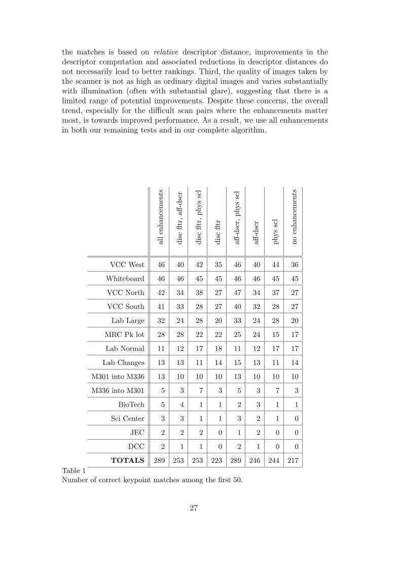
the matches is based on relative descriptor distance, improvements in thedescriptor computation and associated reductions in descriptor distances donot necessarily lead to better rankings. Third, the quality of images taken bythe scanner is not as high as ordinary digital images and varies substantiallywith illumination (often with substantial glare), suggesting that there is alimited range of potential improvements. Despite these concerns, the overalltrend, especially for the difficult scan pairs where the enhancements mattermost, is towards improved performance. As a result, we use all enhancementsin both our remaining tests and in our complete algorithm.

all

enha

ncem

ents

disc

fltr,

aff-d

scr

disc

fltr,

phys

scl

disc

fltr

aff-d

scr,

phys

scl

aff-d

scr

phys

scl

noen

hanc

emen

ts

VCC West 46 40 42 35 46 40 44 36

Whiteboard 46 46 45 45 46 46 45 45

VCC North 42 34 38 27 47 34 37 27

VCC South 41 33 28 27 40 32 28 27

Lab Large 32 24 28 20 33 24 28 20

MRC Pk lot 28 28 22 22 25 24 15 17

Lab Normal 11 12 17 18 11 12 17 17

Lab Changes 13 13 11 14 15 13 11 14

M301 into M336 13 10 10 10 13 10 10 10

M336 into M301 5 3 7 3 5 3 7 3

BioTech 5 4 1 1 2 3 1 1

Sci Center 3 3 1 1 3 2 1 0

JEC 2 2 2 0 1 2 0 0

DCC 2 1 1 0 2 1 0 0

TOTALS 289 253 253 223 289 246 244 217Table 1Number of correct keypoint matches among the first 50.

27

7.2 Refinement

In evaluating the refinement algorithms, we focus on the effectiveness of (a)starting registration from a single keypoint match, (b) region growth duringestimation and refinement, and (c) using image features in the registrationprocess. In testing these, we ran the refinement process on all 50 initial key-point matches.

The results are summarized in Table 2. The first column of results is thenumber of “correct” keypoint matches in the top 50 and is included as a basisfor comparison. The second column, “no reg grow” indicates that there is noregion growth and no image feature correspondences are used. In other words,robust ICP is run scan-wide starting from the initial estimate generated fromthe single keypoint match. The third column indicates that image featurecorrespondences were added, but region growth was still not used. In thefourth and fifth columns, region growth was added.

As before, we make several important observations about these results:

• Clearly, the addition of both image features and region growth substantiallyimproves the number of successful alignments, with region growth playingthe more substantial role. More importantly, adding region growth allowsthe alignment of three of the most challenging pairs. However, we note thatrobust ICP initialized from a single match can accurately align the scans ina surprising number of cases.• Using image feature correspondences is most helpful on scans involving sub-

stantial planar regions (“Whiteboard” and “Lab Changes”). In most otherscans, the effect of image features is negligible. This is partially due to thefact that variations in surface orientation generate constraints in similardirections to the image-feature constraints, making the image features lessnecessary. Another reason is that the low image quality renders the imagefeature constraints less reliable.• The total number of successful final alignments is larger than the number of

correct keypoint matches. This means not only that nearly all initializationsfrom these matches are refined to correct final estimates, but also that somematches that are too far off to be considered correct are actually refined toa correct final estimate. More than anything, this demonstrates the powerof using image features and region growth during the refinement stage.

An additional experiment was performed to determine how well the initial-ization and refinement stages perform as the amount of noise in the scansincreases. We chose five scan pairs representing a range of difficulties, andadded independent, normally-distributed noise to each measurement along itsline of sight. We then ran the algorithm on the resulting scans. Figure 11 plots

28

#kp

tm

atch

es

nore

ggr

ow

nore

ggr

ow+

img

ft

reg

grow

reg

grow

+im

gft

VCC West 46 23 20 47 47

Whiteboard 46 18 36 12 38

VCC North 42 27 19 43 43

VCC South 41 11 21 42 42

Lab Large 32 29 16 32 31

MRC Pk lot 28 9 19 29 30

Lab Normal 11 11 15 19 17

Lab Changes 13 2 14 6 14

M301 into M336 13 16 15 19 18

M336 into M301 5 4 7 6 7

BioTech 5 0 0 1 2

Sci Center 3 0 0 3 3

JEC 2 2 2 2 2

DCC 2 0 0 2 3

TOTALS 289 152 184 263 297Table 2Number of correct alignments produced by the refinement stage when applied tothe top 50 keypoint matches.

the number of initial estimates in the top 50 that the algorithm refines to acorrect transformation as the standard deviation of the added noise increasesfrom 0 to 5 cm (recall that the noise in the scanner is 2 mm). The resultsclearly demonstrate that adding noise to the scans does not substantially af-fect the number of successful registrations. There is a noticeable downwardtrend for several of the scan pairs, mostly on the easier pairs. However, sincethe algorithm only needs a single success, the decrease in the easier scans isinsignificant. Furthermore, the more difficult scans were not greatly affectedby the noise, because their difficulty lies in initialization and not in refinement.

29

Fig. 11. Investigating the effect of additional noise on the performance of the algo-rithm. The number of registration successes in the top 50 initializations is plottedas a function of the standard deviation of the added noise variance for five repre-sentative scan pairs. The additional noise has little effect on the overall power ofthe algorithm because only a single success is needed per scan pair.

7.3 Decision

A linear discriminant combining the seven decision measures was trained usingsix of the scan pairs and the top 50 keypoint match refinements, each comparedto the manually-verified transformation. The results were then tested on all 14pairs, again using the top 50 matches and refinements for all pairs as the basisfor testing. Out of the resulting 700 alignments, there were 3 false negatives,no false positives, and 294 true positives. Unfortunately, as discussed above,two of the false negatives are on the BioTech scan and these are the only twoalignments. Therefore, we cannot claim that this scan was aligned.

When one or more of the measures is removed and the linear discriminant isretrained, performance degrades. Results for these experiments are summa-rized in Table 3. The first four rows of results measure the performance ofthe basic building blocks of the decision criteria, including from top to bot-tom (1) using position accuracy, PAR only, (2) using both range criteria, PAR

and AAR, and the stability measure, ST, (3) using the image-feature-basedcriteria, PAI and AAI , and the stability measure, ST, and (4) just using theboundary measures, BT1 and BT2. Row (1) shows that using the alignmentaccuracy measure alone produces a significant number of false positives, whilerow (4) shows that the boundary measures alone have nearly equivalent per-formance to alignment accuracy. Both are insufficient overall. The remainingrows show, in order, (5) leaving out only the boundary measures, (6) leavingout only the image-feature measures, (7) leaving out only the range measures,and (8) using all measures. It is clear from these results that all criteria are

30

Table 3Verification results of total number of false positives, false negatives, true positives,and true negatives over all scans in Top 50.

Measures Used False Pos. False Neg. True Pos. True Neg.

PAR 19 34 263 384

PAR, AAR, ST 2 106 191 401

PAI , AAI , ST 68 44 253 335

BT1, BT2 22 43 254 381

all but BT1 and BT2 4 8 289 399

all but PAI , AAI 8 7 290 395

all but PAR and AAR 28 7 290 375

all 0 3 294 403

needed, including both the image-feature measures and boundary measures.In addition, it is interesting to note that the image features play a significantoverall role, as can be seen by comparing rows (6) and (8) of the results.

7.4 Performance

The time that it takes to align two preprocessed scan pairs is mainly dependenton the rank of the first initialization that can be refined to a verified alignment.For our experiments, 9 of 14 scan pairs are correctly aligned and verified onthe first ranked initialization. The other four first successes are on the 2nd,6th, 8th, and 37th ranked initializations. It should be noted that many of thefailure refinements before the first success are quickly terminated because ofextremely poor initialization.

We evaluated the performance of the algorithm on our full dataset using aPC with a 3.2GHz Pentium 4 processor and 2 gigabytes of RAM. The sizesof the scans range from 13K to 1.2M points and 2K to 73K intensity features.The preprocessing step of the algorithm is currently the slowest, taking from2.5min up to 10.7min per scan, largely because of large number of overlapping,redundant and sometimes useless images produced by the scanner — we arecurrently working on dramatic speed improvements here. The keypoint match-ing and initialization calculation takes on average 26.4s. The average runningtime of a single registration and verification over all scans is 11.5s with an8.7s standard deviation. Finally, the median time from initialization until theverification detects a successful alignment is 8.7s. Of the four scans whose firstsuccess is not on the first keypoint match the total registration times are 1.9s,2.7min, 1.5min, and 10.2min. Many steps of the algorithm can be trivially par-

31

allelized, which would decrease registration time on multiprocessor machines,especially when the first successful alignment is poorly ranked.

8 Conclusion

We have presented a three-stage algorithm for fully automated 3D rigid reg-istration of combined range/intensity scans that is extremely effective in thepresence of substantial viewpoint differences and structural changes betweenscans. The algorithm succeeds through the combination of (a) the matchingof intensity keypoints that have been backprojected onto range scans, (b) theinitialization of registration estimates from single keypoint matches, (c) an es-timation and refinement procedure that combines robust ICP, region growthand a novel combination of intensity feature and range point correspondences,and (d) a decision criteria that includes measures of positional and orienta-tion alignment accuracy, stability, and a novel boundary-based measure, allcombined using a linear discriminant trained from a subset of the test data.

While the primary contributions of our work are the overall algorithm andits demonstrated effectiveness, we also have several more specific contribu-tions, including (1) an experimental evaluation of the effectiveness of keypointmatching based on backprojected surface information, (2) adapting the Dual-Bootstrap approach — starting from preliminary alignments between smallregions of the data — for range scan registration, (3) a novel method forcombining constraints based on intensity edges and on range points duringestimation, and (4) novel, sophisticated decision criteria for automatically de-termining when two scans are well-aligned despite structural changes.

In terms of the individual stages of our algorithm, we can conclude from ourexperiments that:

• Matching of backprojected keypoints which have been affine-corrected basedon the 3D planar surface is an improvement over matching the keypointsbased on image information algorithm alone. However, the improvementsare not as dramatic as might be expected. The most important effect is inthe most difficult scans where only a small number of correct matches areobtained. Further improvements may be possible using a better estimationof viewpoint-invariant scale.• Region growth and the use of image-feature correspondences both play an

important role in registration, especially on scans of near-planar surfacesand the scan pairs involving the most difficult viewpoint differences andstructural changes.• The combined decision criteria produced no false positives on our data set

and only three false negatives out of 700 tests. While the accuracy measures

32

are important, our novel boundary measures play a crucial role, especiallyon repetitive structures and scans involving structural changes.

As an additional note, we have shown the important role that image featuresplay at all stages of the alignment process, including initialization, refinementand verification. In each stage, backprojected features contribute to the algo-rithm’s success despite substantial viewpoint and/or illumination differencesbetween scans.

Finally, as compared to other approaches, our experiments, including the ad-dition or removal of specific features of our algorithm, have shown that (1)on particularly challenging scan pairs, using matching of backprojected key-points alone [8,57], perhaps followed by robust ICP, is not enough to registerthe scans effectively, (2) just running a robust version of ICP [6, 14, 17, 70] ,initialized using a transformation obtained from a keypoint match, does notconverge to the correct solution reliably, and (3) more sophisticated decisioncriteria [32] than just using alignment error are indeed necessary.

The weakest point of our algorithm is initialization, since we have shownthat once an initial estimate is obtained, region growth and re-estimationnearly always converge to a correct alignment. One area of future investigation,therefore, is new methods for initialization, most likely using range data inaddition to image data [33, 40]. Preliminary results along these lines werepresented in [37]. Aside from initialization, the next stage of our research isextending the algorithm to multiscan registration and automatic detection ofstructural changes. Here the decision criteria will be even more important,as shown in [32] for static scenes, perhaps necessitating more sophisticatedmeasures and non-linear classifiers.

A Modeling Variances in Correspondences

Recall that the variance in a scan point correspondence is modeled as σ2i,j =

k2c (σ2

i + σ2j ), with σ2

i and σ2j being the previously-estimated feature position

variances and kc being an unknown constant multiplier (Equation 8). We usethe fact that kc is the same for all correspondences to estimate its value for eachset of correspondences and transformation parameters. For a correspondencebetween Pi and Qj, let di,j = (T(Pi; Θ) − Qj)

>ηj be the signed normaldistance measured in the fixed scan’s coordinate system. Suppose the valuesof di,j are each normally-distributed, with variance σ2

i,j. Although σ2i,j varies

across the matches, the values di,j/√σ2

i + σ2j are i.i.d. with variance k2

c . Since kc

is the only unknown, we can form the set of values di,j/√σ2

i + σ2j and robustly

compute the variance to estimate kc. In the very first iteration of matching in

33

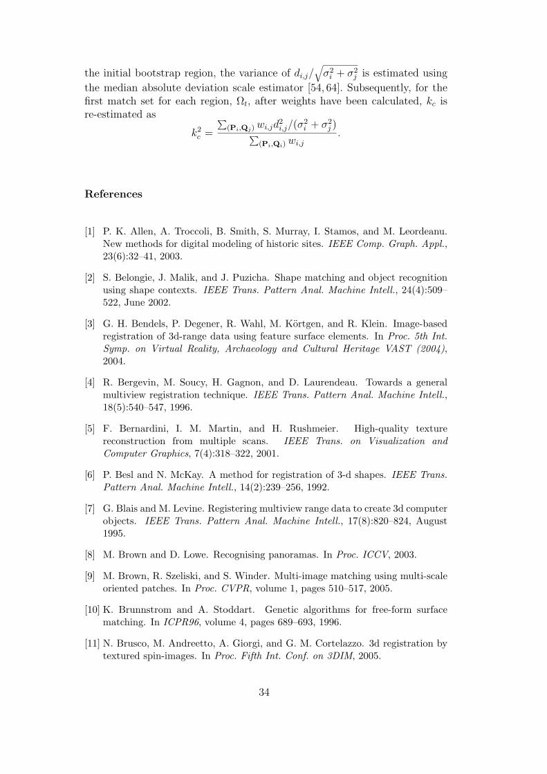
the initial bootstrap region, the variance of di,j/√σ2

i + σ2j is estimated using

the median absolute deviation scale estimator [54, 64]. Subsequently, for thefirst match set for each region, Ωt, after weights have been calculated, kc isre-estimated as

k2c =

∑(Pi,Qj)wi,jd

2i,j/(σ

2i + σ2

j )∑(Pi,Qi)wi,j

.

References

[1] P. K. Allen, A. Troccoli, B. Smith, S. Murray, I. Stamos, and M. Leordeanu.New methods for digital modeling of historic sites. IEEE Comp. Graph. Appl.,23(6):32–41, 2003.

[2] S. Belongie, J. Malik, and J. Puzicha. Shape matching and object recognitionusing shape contexts. IEEE Trans. Pattern Anal. Machine Intell., 24(4):509–522, June 2002.

[3] G. H. Bendels, P. Degener, R. Wahl, M. Kortgen, and R. Klein. Image-basedregistration of 3d-range data using feature surface elements. In Proc. 5th Int.Symp. on Virtual Reality, Archaeology and Cultural Heritage VAST (2004),2004.

[4] R. Bergevin, M. Soucy, H. Gagnon, and D. Laurendeau. Towards a generalmultiview registration technique. IEEE Trans. Pattern Anal. Machine Intell.,18(5):540–547, 1996.

[5] F. Bernardini, I. M. Martin, and H. Rushmeier. High-quality texturereconstruction from multiple scans. IEEE Trans. on Visualization andComputer Graphics, 7(4):318–322, 2001.

[6] P. Besl and N. McKay. A method for registration of 3-d shapes. IEEE Trans.Pattern Anal. Machine Intell., 14(2):239–256, 1992.

[7] G. Blais and M. Levine. Registering multiview range data to create 3d computerobjects. IEEE Trans. Pattern Anal. Machine Intell., 17(8):820–824, August1995.

[8] M. Brown and D. Lowe. Recognising panoramas. In Proc. ICCV, 2003.

[9] M. Brown, R. Szeliski, and S. Winder. Multi-image matching using multi-scaleoriented patches. In Proc. CVPR, volume 1, pages 510–517, 2005.

[10] K. Brunnstrom and A. Stoddart. Genetic algorithms for free-form surfacematching. In ICPR96, volume 4, pages 689–693, 1996.

[11] N. Brusco, M. Andreetto, A. Giorgi, and G. M. Cortelazzo. 3d registration bytextured spin-images. In Proc. Fifth Int. Conf. on 3DIM, 2005.

34

[12] R. J. Campbell and P. J. Flynn. A survey of free-form object representationand recognition techniques. Comput. Vis. Image Und., 81:166–210, Feb. 2001.

[13] C. Chao and I. Stamos. Semi-automatic range to range registration: a feature-based method. In Proc. Fifth Int. Conf. on 3DIM, 2005.

[14] Y. Chen and G. Medioni. Object modeling by registration of multiple rangeimages. IVC, 10(3):145–155, 1992.

[15] C. Chua and R. Jarvis. 3d free-form surface registration and object recognition.Int. J. Comp. Vis., 17(1):77–99, 1996.

[16] C. Chua and R. Jarvis. Point signatures: A new representation for 3d objectrecognition. Int. J. Comp. Vis., 25:63–85, 1997.

[17] G. Dalley and P. Flynn. Pair-wise range image registration: A study in outlierclassification. Comput. Vis. Image Und., 87:104–115, 2002.

[18] R. O. Duda, P. E. Hart, and D. G. Stork. Pattern Classification. John Wileyand Sons, 2001.

[19] J. Feldmar, J. Declerck, G. Malandain, and N. Ayache. Extension of the ICPalgorithm to nonrigid intensity-based registration of 3d volumes. Comput. Vis.Image Und., 66(2):193–206, May 1997.

[20] W. T. Freeman and E. H. Adelson. The design and use of steerable filters.IEEE Trans. Pattern Anal. Machine Intell., 13(9):891–906, September 1991.

[21] A. Frome, D. Huber, R. Kolurri, T. Buelow, and J. Malik. Recognizing objectsin range data using regional point descriptors. In Proc. Eigth ECCV, 2004.

[22] N. Gelfand, L. Ikemoto, S. Rusinkiewicz, and M. Levoy. Geometrically stablesampling for the ICP algorithm. In Proc. Fourth Int. Conf. on 3DIM, pages260–267, 2003.

[23] N. Gelfand, N. J. Mitra, L. J. Guibas, and H. Pottmann. Robust globalregistration. In Eurographics Symposium on Geometry Processing, 2005.

[24] G. Godin, D. Laurendeau, and R. Bergevin. A method for the registration ofattributed range images. In Proc. Third Int. Conf. on 3DIM, pages 179–186,2001.

[25] L. V. Gool, T. Moons, and D. Ungureanu. Affine/ photometric invariants forplanar intensity patterns. In Proc. 4th ECCV, 1996.

[26] S. Granger and X. Pennec. Multi-scale EM-ICP: A fast and robust approachfor surface registration. In Proc. Seventh ECCV, pages 418–432, 2002.

[27] C. Harris and M. Stephens. A combined corner and edge detector.In Proceedings of The Fourth Alvey Vision Conference, pages 147–151,Manchester, UK, 1988.

[28] R. Hartley and A. Zisserman. Multiple View Geometry. Cambridge UniversityPress, 2000.

35

[29] K. Higuchi, M. Hebert, and K. Ikeuchi. Building 3-d models from unregisteredrange images. GMIP, 57(4):315–333, 1995.

[30] P. W. Holland and R. E. Welsch. Robust regression using iteratively reweightedleast-squares. Commun. Statist.-Theor. Meth., A6:813–827, 1977.

[31] E. Horn and N. Kiryati. Toward optimal structured light patterns. IVC,17(2):87–97, 1999.

[32] D. F. Huber and M. Hebert. Fully automatic registration of multiple 3d datasets. IVC, 21:637–650, 2003.

[33] A. Johnson and M. Hebert. Surface matching for object recognition in complex3-dimensional scenes. IVC, 16(9-10):635–651, July 1998.

[34] A. Johnson and S. Kang. Registration and integration of textured 3-d data.IVC, 17(2):135–147, 1999.

[35] A. E. Johnson and M. Hebert. Using spin images for efficient object recognitionin cluttered 3d scenes. IEEE Trans. Pattern Anal. Machine Intell., 21(5):433–449, 1999.

[36] T. Kadir, A. Zisserman, and M. Brady. An affine invariant salient regiondetector. In Proc. Eigth ECCV, 2004.

[37] B. J. King, T. Malisiewicz, C. V. Stewart, and R. J. Radke. Registration ofmultiple range scans as a location recognition problem: Hypothesis generation,refinement and verification. In Proc. Fifth Int. Conf. on 3DIM, pages 180–187,2005.

[38] M. Levoy, K. Pulli, B. Curless, S. Rusinkiewicz, S. Anderson, J. Davis,J. Ginsberg, J. Shade, and D. Fulk. The Digital Michelango Project: 3d scanningof large statues. In SIGGRAPH, pages 131–144, New Orleans, July 2000.

[39] D. G. Lowe. Distinctive image features from scale-invariant keypoints. Int. J.Comp. Vis., 60(2):91–110, November 2004.

[40] A. Makadia, A. Patterson IV, and K. Daniilidis. Fully automatic registrationof 3d point clouds. In Proc. CVPR, New York, NY, USA, 2006.

[41] J. Matas, O. Chum, M. Urban, and T. Pajdla. Robust wide-baseline stereofrom maximally stable extremal regions. IVC, 22(10):761–767, Sept. 2004.

[42] C.-H. Menq, H.-T. Yau, and G.-Y. Lai. Automated precision measurementof surface profile in CAD-directed inspection. IEEE Trans. on Robotics andAutomation, 8(2):268–278, 1992.

[43] A. Mian, M. Bennamoun, and R. Owens. A novel representation and featurematching algorithm for automatic pairwise registration of range images. Int. J.Comp. Vis., 66(1):19–40, 2006.

[44] K. Mikolajczyk and C. Schmid. Scale and affine invariant interest pointdetectors. Int. J. Comp. Vis., 60(1):63–86, 2004.

36

[45] K. Mikolajczyk and C. Schmid. A performance evaluation of local descriptors.IEEE Trans. Pattern Anal. Machine Intell., 27(10):1615–1630, 2005.

[46] K. Mikolajczyk, T. Tuytelaars, C. Schmid, A. Zisserman, J. Matas,F. Schaffalitzky, T. Kadir, and L. V. Gool. A comparison of affine regiondetectors. Int. J. Comp. Vis., 65(1–2):43–72, 2005.

[47] N. J. Mitra, N. Gelfand, H. Pottmann, and L. Guibas. Registration ofpoint cloud data from a geometric optimization perspective. In EurographicsSymposium on Geometry Processing, 2004.

[48] V.-D. Nguyen, V. Nzomigni, and C. Stewart. Fast and robust registration of 3dsurfaces using low curvature patches. In Proc. 2nd Int. Conf. on 3DIM, pages201–208, 1999.

[49] I. S. Okatani and A. Sugimoto. Registration of range images that preserveslocal surface structures and color. In Proc. 3DPVT, 2004.

[50] H. Pottmann, Q.-X. Huang, Y.-L. Yang, and S.-M. Hu. Geometry andconvergence analysis of algorithms for registration of 3d shapes. Int. J. Comp.Vis., 67(3):277–296, May 2006.

[51] K. Pulli. Multiview registration for large data sets. In Proc. 2nd Int. Conf. on3DIM, pages 160–168, 1999.

[52] K. Pulli, S. Piiroinen, T. Duchamp, and W. Stuetzle. Projective surfacematching of colored 3d scans. In Proc. Fifth Int. Conf. on 3DIM, 2005.

[53] G. Roth. Registering two overlapping range images. In Proc. 2nd Int. Conf. on3DIM, pages 191–200, 1999.

[54] P. J. Rousseeuw. Least median of squares regression. J. Amer. Stat. Assoc.,79:871–880, 1984.

[55] S. Rusinkiewicz and M. Levoy. Efficient variants of the ICP algorithm. In Proc.Third Int. Conf. on 3DIM, pages 224–231, 2001.

[56] J. Salvi, C. Matabosch, D. Fofi, and J. Forest. A review of recent range imageregistration methods with accuracy evaluation. IVC, 26, 2006.

[57] J. K. Seo, G. C. Sharp, and S. W. Lee. Range data registration usingphotometric features. In Proc. CVPR, 2005.

[58] G. Sharp, S. Lee, and D. Wehe. ICP registration using invariant features. IEEETrans. Pattern Anal. Machine Intell., 24(1):90–102, 2002.

[59] G. Sharp, S. Lee, and D. Wehe. Multiview registration of 3d scenes byminimizing error between coordinate frames. IEEE Trans. Pattern Anal.Machine Intell., 26(8):1037–1050, 2004.

[60] L. Silva, O. R. P. Bellon, and K. L. Boyer. Enhanced, robust genetic algorithmsfor multiview range image registration. In 3DIM, pages 268–275, 2003.

37

[61] I. Stamos and M. Leordeanu. Automated feature-based range registration ofurban scenes of large scale. In Proc. CVPR, pages II:555–561, 2003.

[62] F. Stein and G. Medioni. Structural indexing: Efficient 3-d object recognition.IEEE Trans. Pattern Anal. Machine Intell., pages 1198–1204, 1992.

[63] C. Stewart, C.-L. Tsai, and B. Roysam. The Dual-Bootstrap Iterative ClosestPoint algorithm with application to retinal image registration. IEEE Trans.Med. Imag., 22(11):1379–1394, 2003.

[64] C. V. Stewart. Robust parameter estimation in computer vision. SIAM Rev.,41(3):513–537, 1999.

[65] C. V. Stewart. Uncertainty-driven, point-based image registration. In Y. C.Nikos Paragios and O. Faugeras, editors, Handbook of Mathematical Models inComputer Vision, pages 221–236. Springer, 2006.

[66] J. Vanden Wyngaerd and L. Van Gool. Automatic crude patch registration:Toward automatic 3d model building. Comput. Vis. Image Und., 87:8–26, 2002.

[67] J. Vanden Wyngaerd and L. Van Gool. Combining texture and shape forautomatic crude patch registration. In Proc. Fourth Int. Conf. on 3DIM, pages179–186, 2003.

[68] S. Weik. Registration of 3-d partial surface models using luminance and depthinformation. In Proc. Int. Conf. on 3DIM, pages 93–100, 1997.

[69] G. Yang, C. V. Stewart, M. Sofka, and C.-L. Tsai. Alignment of challengingimage pairs: Refinement and region growing starting from a single keypointcorrespondence. IEEE Trans. Pattern Anal. Machine Intell., 2007. Acceptedfor publication.

[70] Z. Zhang. Iterative point matching for registration of free-form curves andsurfaces. Int. J. Comp. Vis., 13(2):119–152, 1994.

38