
Regionalism versus Globalization in the Americas - Agricultural and
47
10/28/2001 1 DRAFT – Do Not Quote Regionalism versus Globalization in the Americas: Empirical Evidence on Opportunities and Challenges David Roland-Holst † and Dominique van der Mensbrugghe October, 2001 ABSTRACT Trade liberalization across the Americas holds the potential to substantially improve living standards and present a successful model of North-South regionalism. In this paper, we use a global CGE model to assess the effects of such an arrangement for both member and non-member economies. We also evaluate a number of other issues, including incentive compatibility of the regional agreement for individual members and its structural compatibility with the larger agenda of global trade liberalization. Our results support the notion that regionalism in the Americas is beneficial to member economies, but we note important ways in which it may diverge from the path to global free trade. Generally speaking, our results reveal the complexity of adjustments and indirect effects arising from large trade initiatives of this kind. This serves to remind policy makers of the advantage of detailed empirical analysis over simplified theory, general rules of thumb, or intuition alone. † Paper presented at the international symposium on “Impacts of Trade Liberalization Agreements on Latin America and the Caribbean,” sponsored by the Inter-American Development Bank and the Centre d’Etudes Prospectives et d’Information Internationales, November 5-6, Inter-American Development Bank, Washington, D.C. David Roland-Holst is the James Irvine Professor of Economics at Mills College and Dominique van der Mensbrugghe is a Senior Economist at the World Bank. Opinions expressed here are those of the authors and should not be attributed to their affiliated institutions.
Transcript of Regionalism versus Globalization in the Americas - Agricultural and

10/28/2001 1 DRAFT – Do Not Quote
Regionalism versus Globalization in the Americas: Empirical Evidence on Opportunities and Challenges
David Roland-Holst†
and
Dominique van der Mensbrugghe
October, 2001
ABSTRACT Trade liberalization across the Americas holds the potential to substantially improve living standards and present a successful model of North-South regionalism. In this paper, we use a global CGE model to assess the effects of such an arrangement for both member and non-member economies. We also evaluate a number of other issues, including incentive compatibility of the regional agreement for individual members and its structural compatibility with the larger agenda of global trade liberalization. Our results support the notion that regionalism in the Americas is beneficial to member economies, but we note important ways in which it may diverge from the path to global free trade. Generally speaking, our results reveal the complexity of adjustments and indirect effects arising from large trade initiatives of this kind. This serves to remind policy makers of the advantage of detailed empirical analysis over simplified theory, general rules of thumb, or intuition alone.
† Paper presented at the international symposium on “Impacts of Trade Liberalization Agreements on
Latin America and the Caribbean,” sponsored by the Inter-American Development Bank and the Centre d’Etudes Prospectives et d’Information Internationales, November 5-6, Inter-American Development Bank, Washington, D.C. David Roland-Holst is the James Irvine Professor of Economics at Mills College and Dominique van der Mensbrugghe is a Senior Economist at the World Bank. Opinions expressed here are those of the authors and should not be attributed to their affiliated institutions.
10/28/2001 2 DRAFT – Do Not Quote
1. Introduction
Two decades of regional initiatives have changed the landscape of trade relations
in the Americas. During this period, the region has evolved from an eclectic mosaic of
inward, outward, and post-colonial policy regimes toward a more harmonious blend of
negotiated strategies, giving rise to free trade agreements that set new standards for
North-South and South-South regionalism. With the realization of the NAFTA and
MERCOSUR, economies of the Americas are seeing new patterns of specialization
emerge from more open multilateralism, and this experience is inspiring ambitious plans
to extend free trade across two continents.
In this paper, we use a global CGE model to evaluate several aspects of more
liberal trade across the Americas. In the first instance, we assess the consequences for
individual country trade and real GDP growth when intra-regional import tariffs are
abolished in a Free Trade Across the Americas Agreement (FTAA). As expected, our
results indicate significant long term aggregate gains for member countries, but more
dramatic (in percentage terms) structural adjustments ensuing at the sectoral level. We
also note trade diversion away from extra-regional partners equal to about half the total
growth in intra-regional trade.
Taking the regional perspective as our starting point, we then compare it with two
other reference cases, globalization and unilateralism. Considered as worldwide tariff
abolition, we find that global trade liberalization (GTL) would increase overall trade
more that ten times as much as the FTAA, and trade growth for the regional economies
would be about five times greater. In terms of aggregate real GDP, the regional
economies would experience about double the benefit of FTAA under GTL. From this we
infer that the main impetus toward regionalism is its relative certainty and expedience by
comparison to WTO-based GTL. In other words, the risk-adjusted present value of the
FTAA is higher for regional members. To the extent that and FTAA and GTL are not

10/28/2001 3 DRAFT – Do Not Quote
mutually exclusive, one might also advocate “intermediate regionalism” for the
precedence, institution building and standard setting it confers on member countries.1
A long debate has been carried in the trade literature about the incentive
compatibility of regional agreements, and we examine also this issue below in the context
of the Americas. The basic argument is that, for prospective members of a regional trade
liberalization (RTL) agreement, unilateral trade liberalization (UTL) usually dominates
the RTL and thus the agreement must be designed to include special incentives. This
assertion has been supported with highly simplified theoretical models (3 countries, 2-3
goods), that take no account of terms-of-trade effects or more complex patterns of
adjustment. Our CGE model captures just such effects, and does so in a much more
disaggregated framework. Furthermore, our results indicate that the RTL incentive
problem is empirically vacuous. In no case that we examine for the Americas does
unilateralism even approach the benefits of multilateral liberalization, either at the
regional or global level. Thus we conclude that the FTAA agenda should be sustainable
on basic voluntary principles of market openness.
Whether or not the global or unilateral regimes are in fact compatible with
regionalism is another matter, however, and we also examine this issue in the present
paper. More precisely, comparing aggregate national gains from GTL, RTL, and UTL
reveals nothing about the detailed structural adjustments ensuing from these policy
regimes. These adjustments are of paramount interest to policy makers, however, since
they will exert a strong influence on political evolution, and it is precisely such detailed
structural effects, that CGE models are designed to elucidate. For this reason, we
compare the three types of trade regime in terms of a concept we call structural
congruence (defined precisely below), reflecting the similarity in patterns of real output
adjustment ensuing from different policies.
Our empirical results indicate that, for the majority of member countries, FTAA
type regionalism differs sharply from GTL and UTL in terms of both trade and sectoral
output adjustment, and in many cases we see significant reversals. This implies two
1 These fringe benefits are espoused by a variety of authors, and the general issues are synthesized nicely in
World Bank (2000). Compare also Hoekman adn Leidy (1993) and Lawrence (1996).
10/28/2001 4 DRAFT – Do Not Quote
important things for policy makers. 1) There is no first-mover advantage for countries in
the regional context, meaning they will likely face additional adjustment costs it they
liberalize “ahead” of the regional agenda. 2) There are important ways in which an FTAA
agenda is structurally inconsistent with broader globalization. This portends nontrivial
adjustment costs and political economy considerations that can be expected impede
progress from RTL to GTL.
The path to regionalism in the Americas has been laid out, largely paved with
agreements in fact or in principle and, in many places, is already well-trodden. Whether
or not it points toward or diverges from the path to globalization, it is already conferring
gains on its members and can be expected to do more of this with regional extension and
deepening. It is clear from our results, however, that more attention to the structural
details of liberalization, adjustment, and growth will be needed to realize the full
potential of regional trade and to facilitate an eventual transition to more liberal global
trade. Empirical simulation models of the kind presented here can support this evolving
policy in essential ways, identifying both the opportunities and challenges that lie ahead
for more open multilateralism.
In the next section, we give a brief overview of the global CGE model. This is
followed in section 3 by discussion of the baseline data and forward scenario to which the
model was calibrated. Section 4 presents the basic results of the paper, followed by
concluding remarks in Section 5.
2. Model Summary This paper uses a version of the LINKAGE Model, a global, multi-region, multi-
sector, dynamic applied general equilibrium model.2 The base data set—GTAP3 Version
5.0—is defined across 66 country/region groupings, and 57 economic sectors. For this
paper, the model has been defined for an aggregation of 16 country/regions and 18
2 The LINKAGE model is directly inspired by RUNS Model (see Burniaux and van der Mensbrugghe,
1994), and the OECD GREEN Model (see van der Mensbrugghe, 1994). Full model specification is available from the authors.
3 GTAP refers to the Global Trade Analysis Project based at Purdue University. For more information see Hertel, 1997.

10/28/2001 5 DRAFT – Do Not Quote
sectors including sectors of importance to the poorer developing countries—grains,
textiles, and apparel. The regional and sectoral concordances can be found in Tables 2.1
and 2.2. The remainder of this section outlines briefly the main characteristics of supply,
demand, and the policy instruments of the model.
2.1. Production
All sectors are assumed to operate under constant returns to scale and perfect
competition. Production in each sector is modeled by a series of nested CES production
functions which are intended to represent the different substitution and complementarity
relations across the various inputs in each sector. There are material inputs which
generate the input/output table, as well as factor inputs representing value added.
Three different production archetypes are defined in the model—crops, livestock,
and all other goods and services. The CES nests of the three archetypes are graphically
depicted in Figures A-1 through A-3. Within each production archetype, sectors will be
differentiated by different input combinations (share parameters) and different
substitution elasticities. The former are largely determined by base year data, and the
latter are given values by the modeler.
The key feature of the crop production structure is the substitution between
intensive cropping versus extensive cropping, i.e. between fertilizer and land (see
Figure A-1).4 Livestock production captures the important role played by feed versus
land, i.e. between ranch- versus range-fed production (see Figure A-2).5 Production in
the other sectors more closely matches the traditional role of capital/labor substitution,
with energy introduced as an additional factor of production (see Figure A-3).
In each period, the supply of primary factors—capital, labor, and land—is
usually predetermined. However, the supply of land is assumed to be sensitive to the
contemporaneous price of land. Land is assumed to be partially mobile across agricultural
4 In the original GTAP data set, the fertilizer sector is identified with the crp sector, i.e. chemicals, rubber,
and plastics. 5 Feed is represented by three agricultural commodities in the base data set: wheat, other grains, and oil
seeds.

10/28/2001 6 DRAFT – Do Not Quote
sectors. Given the comparative static nature of the simulations which assumes a longer
term horizon, both labor and capital are assumed to be perfectly mobile across sectors
(though not internationally).6
Model current specification has an innovation in the treatment of labor resources.7
The GTAP data set identifies two types of labor skills—skilled and unskilled. Under the
standard specification, both types of labor are combined together in a CES bundle to form
aggregate sectoral labor demand, i.e. the two types of labor skills are directly
substitutable. In the new specification, a new factor of production has been inserted
which we call human capital. It is combined with capital to form a physical cum human
capital bundle, with an assumption that they are complements. On input, the user can
specify what percentage of the skilled labor factor to allocate to the human capital factor.
Once the optimal combination of inputs is determined, sectoral output prices are
calculated assuming competitive supply (zero-profit) conditions in all markets.
2.2. Consumption and closure rules
All income generated by economic activity is assumed to be distributed to a single
representative household. The single consumer allocates optimally his/her disposable
income among the consumer goods and saving. The consumption/saving decision is
completely static: saving is treated as a “good” and its amount is determined
simultaneously with the demands for the other goods, the price of saving being set
arbitrarily equal to the average price of consumer goods.8
Government collects income taxes, indirect taxes on intermediate and final
consumption, taxes on production, tariffs, and export taxes/subsidies. Aggregate
6 This can be contrasted with, e.g. Fullerton (1983). 7 This feature is not invoked in results reported here. Because of increased interest in labor markets and
human capital in the Latin American context (see e.g. World Bank (2001)), we have developed this modeling capacity and are using it experimentally. For indications about modeling in this context, see Collado et al (1995), Maechler and Roland-Holst (1997), and van der Mensbrugghe (1998).
8 The demand system used in LINKAGE is a version of the Extended Linear Expenditure System (ELES) which was first developed by Lluch (1973). The formulation of the ELES used in LINKAGE is based on atemporal maximization—see Howe (1975). In this formulation, the marginal propensity to save out of supernumerary income is constant and independent of the rate of reproduction of capital.

10/28/2001 7 DRAFT – Do Not Quote
government expenditures are linked to changes in real GDP. The real government deficit
is exogenous. Closure therefore implies that some fiscal instrument is endogenous in
order to achieve a given government deficit. The standard fiscal closure rule is that the
marginal income tax rate adjusts to maintain a given government fiscal stance. For
example, a reduction or elimination of tariff rates is compensated by an increase in
household direct taxation, ceteris paribus.
Each region runs a current-account surplus (deficit) that is fixed (in terms of the
model numéraire). The counterpart of these imbalances is a net outflow (inflow) of
capital, subtracted from (added to) the domestic flow of saving. In each period, the model
equates gross investment to net saving (equal to the sum of saving by households, the net
budget position of the government and foreign capital inflows). This particular closure
rule implies that investment is driven by saving. The fixed trade balance implies an
endogenous real exchange rate. For example, removal of tariffs which induces increased
demand for imports is compensated by increasing exports which is achieved through a
real depreciation.
2.3. Foreign Trade
The world trade block is based on a set of regional bilateral flows. The basic
assumption in LINKAGE is that imports originating in different regions are imperfect
substitutes (see Figure A-4). Therefore in each region, total import demand for each good
is allocated across trading partners according to the relationship between their export
prices. This specification of imports—commonly referred to as the Armington9
specification—implies that each region faces a downward-sloping demand curve for its
exports. The Armington specification is implemented using two CES nests. At the top
nest, domestic agents choose the optimal combination of the domestic good and an
aggregate import good consistent with the agent’s preference function. At the second
9 See Armington, 1969 and compare, e.g. de Melo and Robinson (1989) and Rutherford and Tarr (2001).

10/28/2001 8 DRAFT – Do Not Quote
nest, agents optimally allocate demand for the aggregate import good across the range of
trading partners.10
The bilateral supply of exports is specified in parallel fashion using a nesting of
constant-elasticity-of-transformation (CET) functions. At the top level, domestic
suppliers optimally allocate aggregate supply across the domestic market and the
aggregate export market. At the second level, aggregate export supply is optimally
allocated across each trading region as a function of relative prices.11
Trade variables are fully bilateral and include both export and import
taxes/subsidies. Trade and transport margins are also included, therefore world prices
reflect the difference between FOB and CIF pricing.
2.4. Prices
The LINKAGE model is fully homogeneous in prices, i.e. only relative prices are
identified in the equilibrium solution. The price of a single good, or of a basket of goods,
is arbitrarily chosen as the anchor to the price system. The price (index) of OECD
manufacturing exports has been chosen as the numéraire, and is set to 1.
2.5. Elasticities
Production elasticities are relatively standard and are available from the authors.
Aggregate labor and capital supplies are fixed, and within each economy they are
perfectly mobile across sectors.
10 The GTAP data set allows each agent of the economy to be an Armington agent, i.e. each column of
demand in the input/output matrix is disaggregated by domestic and import demand. (The allocation of imports across regions can only be done at the national level). For the sake of space and computing time, the standard model specification adds up Armington demand across domestic agents and the Armington decomposition between domestic and aggregate import demand is done at the national level, not at the individual agent level.
11 A theoretical analysis of this trade specification can be found in de Melo and Robinson, 1989.
10/28/2001 9 DRAFT – Do Not Quote
3. Baseline Data and Scenario
As has already been mentioned the model is calibrated to a 1997 reference global
database obtained from GTAP Version 5. While these data are generally available to the
research community, we reproduce some of this information in the present section for the
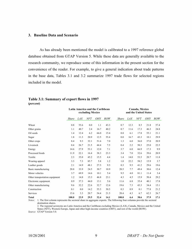
convenience of the reader. For example, to give a general indication about trade patterns
in the base data, Tables 3.1 and 3.2 summarize 1997 trade flows for selected regions
included in the model.
Table 3.1: Summary of export flows in 1997 (percent)
Latin America and the Caribbean
excluding Mexico Canada, Mexico
and the United States
Share LAX NFT OHY ROW Share LAX NFT OHY ROW
Wheat 0.8 55.6 0.0 1.1 43.3 0.7 12.3 8.5 21.8 57.4 Other grains 1.1 40.7 2.4 16.7 40.2 0.7 11.6 17.3 46.3 24.8 Oil seeds 1.4 12.4 6.2 66.0 15.4 0.8 6.1 17.8 55.1 21.1 Sugar 1.8 11.3 20.9 12.5 55.4 0.0 16.7 43.3 10.1 29.9 Other crops 8.4 9.3 32.1 51.6 7.0 1.3 6.0 36.0 37.0 20.9 Livestock 0.4 26.7 21.5 44.4 7.5 0.4 2.2 50.3 25.0 22.5 Energy 14.6 27.9 53.1 12.0 7.1 3.7 6.0 66.9 17.3 9.9 Processed foods 11.9 22.1 16.4 38.3 23.3 3.4 7.0 32.6 39.6 20.9 Textile 2.3 35.0 45.2 15.5 4.4 1.4 14.0 53.5 20.7 11.8 Wearing apparel 3.3 7.3 85.7 5.8 1.2 1.0 22.2 58.2 15.9 3.7 Leather goods 2.1 14.9 48.1 27.5 9.5 0.3 9.5 41.2 29.6 19.6 Basic manufacturing 20.8 33.9 24.5 30.7 10.9 20.5 7.7 49.4 30.6 12.4 Motor vehicles 3.7 69.9 14.6 10.1 5.4 9.5 4.0 81.1 11.4 3.4 Other transportation equipment 1.2 14.8 15.3 46.8 23.1 4.3 4.5 15.9 50.4 29.2 Electronic equipment 0.9 37.3 44.0 13.1 5.6 11.6 6.8 35.4 40.1 17.8 Other manufacturing 9.6 32.2 22.6 32.7 12.6 19.6 7.3 43.3 34.4 15.1 Construction 0.1 0.0 14.2 55.3 30.5 0.3 0.9 0.1 77.8 21.2 Services 15.6 3.3 20.7 54.4 21.5 20.4 4.3 6.7 62.3 26.7 Total 100.0 23.9 29.5 32.4 14.1 100.0 6.4 38.6 37.9 17.1 Notes: 1. The first column represents the sectoral share in aggregate exports. The following four columns provide the sectoral
destination shares. 2. The regional acronyms are Latin America and the Caribbean excluding Mexico (LAX), Canada, Mexico and the United
States (NFT), Western Europe, Japan and other high-income countries (OHY), and rest of the world (ROW). Source: GTAP Version 5.0.

10/28/2001 10 DRAFT – Do Not Quote
Table 3.2: Summary of import flows in 1997 (percent)
Latin America and the Caribbean
excluding Mexico Canada, Mexico
and the United States
Share LAX NFT OHY ROW Share LAX NFT OHY ROW
Wheat 0.8 44.1 48.5 7.4 0.0 0.1 0.0 98.1 0.0 1.9 Other grains 0.8 46.2 46.6 1.0 6.1 0.1 2.9 74.3 3.6 19.2 Oil seeds 0.4 39.6 60.4 0.0 0.0 0.1 9.4 84.6 4.0 1.9 Sugar 0.2 87.1 10.1 2.8 0.0 0.1 56.4 9.1 17.7 16.8 Other crops 1.4 47.7 27.2 6.8 18.3 1.1 37.3 37.0 6.7 19.0 Livestock 0.2 49.4 28.1 17.7 4.8 0.3 4.4 71.5 15.1 9.0 Energy 7.2 46.7 14.8 10.3 28.2 6.4 19.3 36.0 10.4 34.3 Processed foods 4.8 45.9 24.0 27.5 2.7 2.7 11.4 37.4 35.0 16.2 Textile 3.0 22.5 32.1 15.4 30.0 2.1 7.8 33.0 26.2 33.0 Wearing apparel 1.9 10.6 57.2 6.4 25.8 3.1 14.6 17.5 18.8 49.1 Leather goods 0.9 29.4 14.2 11.5 44.9 1.7 9.5 6.1 17.5 66.9 Basic manufacturing 22.0 26.5 34.6 30.8 8.1 18.9 4.3 49.3 33.3 13.2 Motor vehicles 7.8 27.6 23.8 41.3 7.4 11.9 0.7 59.7 37.5 2.0 Other transportation equipment 5.4 2.7 17.2 65.2 14.8 1.8 1.6 34.8 56.9 6.8 Electronic equipment 7.1 3.7 53.2 28.2 14.9 14.5 0.4 26.2 45.5 28.0 Other manufacturing 19.7 13.0 35.0 43.5 8.5 19.8 1.7 39.5 42.4 16.3 Construction 0.1 0.0 10.6 69.1 20.3 0.1 1.6 0.4 68.1 29.9 Services 16.4 2.6 25.7 51.8 19.9 15.1 3.4 8.4 64.2 24.1 Total 100.0 19.8 31.1 35.6 13.4 100.0 4.7 35.5 39.7 20.1 Notes: 1. The first column represents the sectoral share in aggregate imports. The following four columns provide the sectoral
shares by region of origin. 2. The regional acronyms are Latin America and the Caribbean excluding Mexico (LAX), Canada, Mexico and the United
States (NFT), Western Europe, Japan and other high-income countries (OHY), and rest of the world (ROW). Source: GTAP Version 5.0.
Second only to trade flows in their importance for determining the policy
outcomes we consider in this paper are prior patterns of import protection. The next three
tables present this information in different ways to elucidate a variety of perspectives on
trade price distortions. For selected regions, Tables 3.3 and 3.4 give import protection
levels by origin and destination, respectively. This helps reveal asymmetries in market
openness for the aggregate commodity groups in the current database. Table 3.5, on the
other hand, gives a matrix of trade weighted import barriers by country and region,
indicating (fairly significant) asymmetries in overall domestic market access under
current (1997) patterns of trade. Table 3.6 summarizes the country and regional
abbreviations used in tables throughout the paper.

10/28/2001 11 DRAFT – Do Not Quote
It is essential to note, even in passing, that we are not modeling significant
agricultural protection in the present exercise. This means our results will generally
understate the effects of trade liberalization at the aggregate level and do not fully capture
sectoral adjustments, particularly in primary activities. This will be the subject of further
research.12
Table 3.3: Applied tariffs by region of origin (percent)
Latin America and the Caribbean
excluding Mexico Canada, Mexico
and the United States
LAX NFT OHY ROW Total LAX NFT OHY ROW Total
Wheat 6.6 8.3 0.0 .. 7.0 .. 32.1 .. 0.0 31.5 Other grains 12.4 13.9 0.0 14.9 13.2 0.0 20.2 0.0 2.9 15.5 Oil seeds 4.1 6.2 .. .. 5.4 8.6 4.4 0.0 0.0 4.6 Sugar 13.3 12.3 0.0 .. 12.8 46.4 45.0 24.1 51.5 43.1 Other crops 9.2 9.7 7.3 5.4 8.5 13.3 7.4 11.7 15.5 11.5 Livestock 0.0 7.6 0.0 0.0 2.1 0.0 4.1 0.0 0.0 2.9 Energy 6.4 5.0 2.6 4.3 5.2 0.9 0.0 0.7 0.5 0.4 Processed foods 15.5 16.0 17.8 12.2 16.2 12.1 17.4 15.0 11.7 15.0 Textile 14.4 17.3 13.3 13.5 14.9 14.4 0.0 11.3 11.3 7.9 Wearing apparel 17.1 24.9 13.4 14.2 20.5 13.9 0.0 14.1 13.7 11.5 Leather goods 13.6 14.6 8.1 17.0 14.8 8.8 0.0 9.4 15.3 12.8 Basic manufacturing 10.7 9.8 10.2 9.0 10.1 3.0 0.0 3.8 3.6 1.9 Motor vehicles 32.6 22.2 22.6 26.7 25.6 2.9 0.0 3.0 2.1 1.2 Other transportation equipment 11.0 3.7 12.7 9.5 10.6 1.7 0.0 1.5 3.1 1.1 Electronic equipment 9.8 10.5 10.7 12.4 10.8 3.4 0.0 1.4 1.5 1.1 Other manufacturing 12.0 11.5 12.4 14.6 12.2 2.8 0.0 2.8 2.5 1.7 Construction .. 0.0 3.9 0.0 2.7 0.0 0.0 0.0 0.0 0.0 Services 0.0 1.1 0.9 0.8 0.9 0.0 0.0 0.0 0.0 0.0 Total 12.8 10.5 10.1 8.8 10.6 5.9 0.8 2.7 4.1 2.5 Agriculture & food 12.6 12.7 16.0 8.3 13.0 14.9 13.7 14.2 13.1 14.0 Energy 6.4 5.0 2.6 4.3 5.2 0.9 0.0 0.7 0.5 0.4 Textile & apparel 14.7 21.0 12.6 14.5 16.7 13.0 0.0 12.0 13.8 10.8 Other manufacturing 15.2 11.3 13.0 13.0 12.8 2.9 0.0 2.7 2.4 1.5 Other goods & services 0.0 1.1 1.0 0.8 1.0 0.0 0.0 0.0 0.0 0.0 Notes: 1. Tariffs applied by LAX and NFT. The tariffs are weighted by import values. 2. The regional acronyms are Latin America and the Caribbean excluding Mexico (LAX), Canada, Mexico and the United
States (NFT), Western Europe, Japan and other high-income countries (OHY), and rest of the world (ROW). Source: GTAP Version 5.0.
12 See, e.g. OECD (1990), Goldin, Knudsen, and van der Mensbrugghe (1993), and van der Mensbrugghe
and Guerrero (1998) for indications about treatment of agricultural liberalization in this framework.

10/28/2001 12 DRAFT – Do Not Quote
Table 3.4: Applied tariffs by region of destination (percent)
Latin America and the Caribbean
excluding Mexico Canada, Mexico
and the United States
LAX NFT OHY ROW Total LAX NFT OHY ROW Total
Wheat 6.6 .. 64.8 32.6 18.5 8.3 32.1 170.6 34.0 60.6 Other grains 12.4 0.0 47.4 49.6 33.3 13.9 20.2 31.6 90.8 42.6 Oil seeds 4.1 8.6 15.0 66.0 21.1 6.2 4.4 29.8 78.6 34.6 Sugar 13.3 46.4 83.0 17.9 31.6 12.3 45.0 88.9 23.7 37.4 Other crops 9.2 13.3 10.4 34.7 13.0 9.7 7.4 17.6 26.2 15.3 Livestock 0.0 0.0 8.2 0.0 3.7 7.6 4.1 19.9 10.4 9.6 Energy 6.4 0.9 2.2 2.8 2.7 5.0 0.0 0.5 4.1 0.8 Processed foods 15.5 12.1 31.1 38.4 26.4 16.0 17.4 32.8 43.4 29.1 Textile 14.4 14.4 5.9 6.7 12.7 17.3 0.0 7.2 14.7 5.8 Wearing apparel 17.1 13.9 5.5 0.0 13.5 24.9 0.0 10.8 19.7 8.1 Leather goods 13.6 8.8 5.2 2.1 7.9 14.6 0.0 7.6 12.0 6.1 Basic manufacturing 10.7 3.0 1.8 7.2 5.7 9.8 0.0 2.6 9.5 2.8 Motor vehicles 32.6 2.9 6.4 16.3 24.7 22.2 0.0 5.2 15.7 2.1 Other transportation equipment 11.0 1.7 0.5 2.0 2.5 3.7 0.0 1.1 4.3 2.0 Electronic equipment 9.8 3.4 2.4 0.0 5.4 10.5 0.0 2.2 6.0 2.7 Other manufacturing 12.0 2.8 0.5 3.1 4.9 11.5 0.0 2.1 9.6 3.0 Construction .. 0.0 0.0 0.0 0.0 0.0 0.0 0.0 0.0 0.0 Services 0.0 0.0 0.0 0.2 0.1 1.1 0.0 0.0 0.4 0.1 Total 12.8 5.9 8.2 16.2 9.8 10.5 0.8 4.3 9.9 4.3 Agriculture & food 12.6 14.9 22.1 35.8 21.8 12.7 13.7 35.9 45.1 30.3 Energy 6.4 0.9 2.2 2.8 2.7 5.0 0.0 0.5 4.1 0.8 Textile & apparel 14.7 13.0 5.5 3.2 11.8 21.0 0.0 8.3 14.9 6.7 Other manufacturing 15.2 2.9 1.5 5.9 7.3 11.3 0.0 2.3 8.3 2.7 Other goods & services 0.0 0.0 0.0 0.2 0.1 1.1 0.0 0.0 0.3 0.1 Notes: 1. Tariffs faced by exports from LAX and NFT. The tariffs are weighted by import values. 2. The regional acronyms are Latin America and the Caribbean excluding Mexico (LAX), Canada, Mexico and the United
States (NFT), Western Europe, Japan and other high-income countries (OHY), and rest of the world (ROW). Source: GTAP Version 5.0.

10/28/2001 13 DRAFT – Do Not Quote
Table 3.5: Bilateral, Trade Weighted Tariffs (percent) Exporter
Import usa can mex arg bra chl col ven xsm eur rhy jpn chn xea sas row Total hiy liy wsh nft lax
usa 0.4 0.5 4.6 5.2 3.4 7.1 1.1 9.4 2.2 2.8 2.3 5.7 3.8 7.0 2.1 2.4 0.6 3.1 2.9 1.7 3.3 can 0.8 0.5 6.9 4.2 13.3 0.0 1.5 3.2 3.8 5.3 3.7 8.7 3.6 8.9 2.1 2.0 0.8 4.1 4.1 3.6 4.2 mex 1.8 8.2 9.8 8.2 11.7 0.0 7.2 8.3 7.3 9.9 8.7 13.6 9.6 6.5 4.1 3.8 2.0 7.9 8.3 9.9 8.1 arg 9.6 8.7 14.9 15.4 12.8 0.0 0.0 8.2 11.7 7.4 10.9 16.8 12.7 6.1 4.2 11.6 12.6 10.8 11.6 10.1 11.8 bra 10.4 6.1 14.7 21.8 6.8 0.0 5.8 8.1 10.4 7.7 13.9 15.1 13.3 5.3 4.2 11.0 13.5 9.6 12.7 17.7 11.1 chl 9.2 7.7 10.3 9.8 9.5 7.5 11.0 9.0 8.4 6.6 9.1 10.2 8.7 0.0 6.5 8.9 9.4 8.4 8.8 9.3 8.7 col 8.6 1.9 11.8 9.3 9.7 10.0 14.8 14.5 6.0 2.7 12.8 5.0 13.8 0.0 4.1 8.8 8.6 9.0 8.6 8.1 8.6 ven 10.4 15.7 14.8 12.4 15.3 3.3 15.8 10.6 7.3 5.6 15.7 12.0 9.7 0.0 1.9 10.4 11.7 9.0 9.6 11.6 9.1 xsm 11.8 9.1 8.4 10.7 10.9 11.8 10.3 7.9 11.5 9.2 9.4 12.6 13.5 10.3 3.1 4.7 10.6 11.2 10.2 10.6 9.4 10.8
eur 2.7 3.3 3.1 15.9 7.0 4.5 4.2 2.5 10.1 0.5 4.7 3.6 5.7 4.6 7.3 4.4 1.9 3.2 1.8 1.4 5.2 1.2 rhy 2.0 1.4 0.3 4.1 1.6 1.3 0.0 0.0 1.0 2.6 1.5 2.8 2.9 1.5 2.9 0.9 2.1 2.0 2.2 2.3 1.5 2.4 jpn 9.3 19.4 5.0 13.8 11.0 10.0 10.4 0.0 14.6 3.7 10.4 8.6 6.7 10.2 1.8 7.0 10.3 5.8 6.7 10.2 5.9 chn 13.9 22.6 5.9 22.9 36.6 1.0 0.0 0.0 7.3 11.0 15.7 15.2 16.0 9.5 5.3 14.0 16.0 13.6 14.4 15.7 13.8 xea 9.3 3.9 6.1 34.3 11.0 6.6 5.1 0.0 6.8 5.8 7.6 9.8 18.4 9.2 8.0 4.4 8.3 9.2 8.1 8.8 8.0 9.0 sas 15.5 7.6 8.7 25.5 20.7 15.7 7.3 0.0 5.1 18.8 17.4 27.0 27.4 25.3 19.5 24.5 21.0 15.3 21.8 21.0 17.7 21.6 row 8.7 12.7 5.0 25.9 19.0 16.2 4.8 4.3 10.3 11.1 8.7 8.6 14.4 11.0 13.9 8.2 10.3 10.1 10.3 11.1 10.1 11.1
Total 5.1 2.6 1.7 17.4 10.5 6.7 6.7 3.4 9.6 3.1 6.9 6.1 8.3 6.5 8.7 5.1 4.8 4.9 4.7 4.7 6.4 4.4
hiy 2.1 0.5 0.8 17.3 8.9 6.3 6.2 1.7 8.9 3.5 3.4 2.9 6.4 4.4 7.1 2.4 3.2 1.9 3.8 3.9 2.9 4.1 liy 6.2 8.3 5.3 17.5 11.3 6.8 6.9 6.2 10.2 3.0 8.0 7.5 9.1 7.1 9.3 5.5 5.2 6.9 4.9 4.9 8.3 4.5 wsh 5.3 7.6 4.8 16.1 10.7 6.7 5.9 4.7 10.0 1.6 7.9 7.3 8.5 6.7 8.0 4.6 4.3 5.9 4.0 3.9 8.0 3.5 nft 2.3 3.0 5.0 5.3 11.7 6.1 0.0 4.8 5.2 4.0 2.1 3.3 3.6 2.0 3.3 1.4 3.0 2.9 3.0 3.1 2.3 3.3 lax 6.3 8.3 4.8 17.2 10.4 6.9 6.3 4.7 10.5 1.5 9.1 8.7 9.7 8.3 8.6 4.9 4.5 6.8 4.1 4.0 9.2 3.5

10/28/2001 14 DRAFT – Do Not Quote
Table 3.6: Regional Definitions
eur Western Europe rhy Rest of high-income can Canada usa United States jpn Japan chn China xea Rest of East Asia sas South Asia arg Argentina bra Brazil mex Mexico col Colombia ven Venezuela chl Chile xsm Rest of Latin America and the Caribbean row Rest of the World hiy High-income countries liy Low- and middle-income countries wlt World total lac Latin America and the Caribbean lix Developing countries excluding LAC nft NAFTA wsh Western Hemisphere lax Latin America excluding Mexico
As mentioned in the previous section, the dynamic CGE model is calibrated to a
baseline time series reflecting a business-as-usual (BAU) scenario over the period 1997-
2015. For reference, Table 3.7 below presents these baseline values of selected variables
in the initial and terminal years.

10/28/2001 15 DRAFT – Do Not Quote
Table 3.7: Summary of baseline scenario ($1997 billions unless otherwise stated)
High-income
Low- and middle-income
Latin America and the
Caribbean x/ Mexico
Canada, Mexico, and United States
Rest of high income
Rest of the World World total
Aggregate statistics in base year (1997) Real GDP 22,181 6,802 1,587 8,965 13,605 4,827 28,983 Population (millions) 867 4,946 396 396 566 4,456 5,814 Labor force 12,049 2,888 693 5,333 6,825 2,086 14,937 Capital stock1 8,468 3,088 758 3,475 5,226 2,097 11,557 Exports 4,492 1,704 206 1,199 3,409 1,383 6,196 Imports 4,586 1,820 258 1,341 3,346 1,461 6,406 GDP per capita ($1997) 25,575 1,375 4,010 22,648 24,048 1,083 4,985 GDP share (percent of world total) 76.5 23.5 5.5 30.9 46.9 16.7 100.0 Population share (percent of world total) 14.9 85.1 6.8 6.8 9.7 76.7 100.0 Parity index2 513 28 80 454 482 22 100 Aggregate statistics in final year (2015) Real GDP 35,206 14,476 2,757 15,092 20,909 10,925 49,683 Population (millions) 911 6,199 498 464 568 5,580 7,110 Labor force 12,516 3,911 919 6,116 6,555 2,836 16,427 Capital stock 14,850 7,024 1,362 6,379 8,904 5,230 21,875 Exports 7,155 3,591 407 2,111 5,260 2,968 10,745 Imports 7,519 3,642 447 2,310 5,409 2,996 11,161 GDP per capita ($1997) 38,634 2,335 5,535 32,544 36,789 1,958 6,988 GDP share (percent of world total) 70.9 29.1 5.5 30.4 42.1 22.0 100.0 Population share (percent of world total) 12.8 87.2 7.0 6.5 8.0 78.5 100.0 Parity index 553 33 79 466 526 28 100 Average annual growth rate, 1997-2015 (percent)
Real GDP 2.6 4.3 3.1 2.9 2.4 4.6 3.0 Population 0.3 1.3 1.3 0.9 0.0 1.3 1.1 Labor force 0.2 1.7 1.6 0.8 -0.2 1.7 0.5 Capital stock 3.2 4.7 3.3 3.4 3.0 5.2 3.6 Exports 2.6 4.2 3.9 3.2 2.4 4.3 3.1 Imports 2.8 3.9 3.1 3.1 2.7 4.1 3.1 GDP per capita ($1997) 2.3 3.0 1.8 2.0 2.4 3.3 1.9 GDP share3 -5.7 5.7 0.1 -0.6 -4.9 5.3 0.0 Population share3 -2.1 2.1 0.2 -0.3 -1.7 1.8 0.0 Parity index3 39.9 5.8 -1.2 11.4 44.1 6.3 0.0 Notes: 1. Capital stock is normalized to base year prices. 2. Parity index measures the ratio of per capita income relative to the average world per capita income. 3. The share and index numbers represent differences between the base and final years, not the growth rate. Source: GTAP 5.0 and model simulation results. See Hertel (1997) and Ianchovichna and MsDougall (2000) for documentation.

10/28/2001 16 DRAFT – Do Not Quote
4. Simulation Results
Using the multi-country model and baseline information discussed above, we
conducted a series of policy experiments reflecting more liberal trade regimes at the
global, regional, bilateral, and national levels. In particular, in the first pair of
experiments we compare detailed differences between tariff removal within the Americas
and global tariff abolition. The results obtained indicate both the potential rewards of
further liberalization and the very complex incentives facing participants in regional and
global negotiations. Two general results are worthy of emphasis:
• Global trade liberalization (GTL) confers greater aggregate gains, not only
on the world but on each country and sub-region in the Americas.
• Regional trade liberalization (RTL) or free trade across the Americas
(FTAA) would, in the absence of other negotiating initiatives, benefit
member countries in the region but induce significant trade diversion away
from the rest of the world.
While these conclusions (particularly on a bilateral basis) have interesting
implications for trade negotiations, FTAA and globalization are not considered to be
mutually exclusive, and many hope the former will simply provide impetus to be
superceded by the latter. Trade divergence and discrimination (de jure or de facto) induce
real economic adjustments, however, and they can complicate the larger negotiating
environment in nontrivial ways. If the credibility of global free trade is limited, however,
there appear to be substantial incentives to expedite regionalism.13 Unfortunately, as we
shall see later, this may itself undermine global initiative.
At the national level, we also examine unilateral liberalization for a number of
larger economies in Latin America. These results are then compared to a case where
bilateral partners reciprocate, conferring free market access on the country removing all
its tariff barriers. Not surprisingly, these two alternatives differ in important respects,
depending upon prior protection patterns and domestic resource constraints. Although
there are important general characteristics of the individual country scenarios, our results
13 On the former issue, see e.g. Hoekman and Kostecki (1995).

10/28/2001 17 DRAFT – Do Not Quote
suggest that the choice between unilateral and negotiated tariff removal should be made
on a case by case basis. Indeed, unilateral removal would rarely be optimal, but
negotiated liberalization should be informed by more detailed analysis of partner- and
sector-specific trade issues.
4.1. Adjustments in Trade Patterns
Turning to the detailed results, Table 4.1 presents bilateral trade flow adjustments
in response to global tariff removal, expressed in both constant (1997 billions of) dollars
and as percentage changes with respect to the baseline levels forecast for 2015. By the
terminal year of these projections, tariff abolition is estimated to increase global trade by
$1.771 trillion 1997 dollars or 16.5%. At the same time, multilateral liberalization will
create a highly variegated landscape of bilateral trade adjustments, ranging from a
expansion of 274.4% (Brazil’s exports to China) to contraction of -67.1% (Venezuela’s
exports to East Asia). While global trade is expanding by 16.5% in real terms, most non-
OECD countries experience total export growth well in excess of this figure. Latin
American countries in particular see trade rising sharply, with Argentine and Brazilian
exports rising 58% and imports going up by 60% and 50%, respectively.14 Chile,
Colombia, Venezuela, and the Rest of LAC are all above the global average, with only
Mexico below average because of its low rates of prior protection.
While the general impression is one of trade growth, with 216 (84%) of the 256
bilateral flows expanding, some bilateral ties will remain fairly constant or even contract.
Net changes in bilateral trade are the result of shifting relative real exchange rates, which
in turn result from differences in prior protection levels (Table 3.5). Thus it is worth
noting that, even in the case of multilateral tariff abolition, trade diversion still results
because of asymmetries in prior protection patterns. Fortunately, the diversionary effects
are relatively small in this global free trade scenario, and they are far outweighed by trade
creation at each national level and, therefore, in the aggregate.
14 Differences here are due to differences in real exchange rate adjustments. Because of Brazil’s higher
prior protection (Table 3.5), their real exchange rate rises less and the purchasing power of their exports, under the BOP closure constraint, allows a smaller increase in imports.

Table 4.1: Bilateral Trade Flows - Global Trade Liberalization(changes in 2015)
Exporters 1997 BillionsImporters usa can mex arg bra chl col ven xsm eur jpn rhy chn xea sas row TotalUnited States usa .0 -18.1 4.0 -.2 2.0 .6 .3 1.5 6.3 47.8 -1.8 -15.6 66.0 14.7 20.9 21.5 149.9Canada can -18.0 .0 .7 .0 .1 .3 .1 .1 .1 12.6 2.3 .2 7.7 1.7 1.6 2.5 12.0Mexico mex -22.6 .4 .0 .1 2.4 .8 .0 .6 .5 14.9 3.3 1.7 6.7 4.6 1.3 1.9 16.4Argentina arg 3.2 .2 1.3 .0 12.0 1.1 .0 .0 .7 8.0 .4 .2 4.1 1.5 .4 .8 33.9Brazil bra 9.5 .2 2.7 15.9 .0 .3 .0 .6 .9 13.7 2.0 .4 9.1 7.2 .8 3.3 66.6Chile chl 1.3 .1 .7 .2 .6 .0 .1 .1 .5 2.2 .0 -.1 2.0 .4 .0 .3 8.2Colombia col .8 -.1 .5 .0 .1 .1 .0 1.5 .7 .7 .0 -.2 .2 .7 .0 .2 5.2Venezuela ven 1.0 .2 .7 .1 1.0 -.1 .9 .0 .3 .8 .2 -.1 .8 .4 .0 .1 6.4Rest of LAC xsm 10.3 .6 1.5 .8 2.1 1.0 1.2 1.5 .0 4.5 1.5 .1 5.0 .8 .1 .7 36.4Western Europe eur 26.0 12.6 4.2 8.8 11.2 1.8 1.9 .5 18.2 .0 10.6 30.4 72.7 32.2 38.3 175.7 247.8Rest of hi-income jpn 11.1 2.6 1.4 .0 .6 1.2 .3 .0 .8 20.0 .0 14.8 39.6 18.9 6.8 17.4 135.5Japan rhy 12.5 1.0 .5 .2 .4 .4 .1 .0 .4 31.8 3.7 .0 26.4 9.6 6.9 9.3 91.7China chn 30.9 6.0 .3 1.5 16.6 -.6 .0 .0 -1.3 48.3 49.8 41.9 .0 73.2 3.5 7.0 277.0Rest of East Asia xea 26.4 1.3 1.2 .4 .5 .7 .4 -.1 1.2 37.9 29.1 1.5 55.1 .0 7.6 16.6 247.6South Asia sas 4.5 -.1 .0 .4 .3 .1 .1 -.1 -.1 22.0 6.5 -.6 18.1 11.3 .0 32.8 99.3Rest of the World row 29.5 6.2 1.7 6.3 16.2 1.1 .5 .2 4.0 117.4 2.4 2.1 39.6 17.0 29.3 .0 337.3
Total 126.5 13.1 21.3 34.4 65.9 8.8 5.9 6.4 38.0 185.5 110.0 65.0 353.1 261.8 121.7 353.7 1771.1Percentages
United States usa .0 -6.6 2.6 -5.9 9.9 12.1 2.7 9.3 17.8 13.2 -1.2 -12.2 33.8 9.8 67.0 17.4 9.0Canada can -7.8 .0 8.9 8.3 7.2 75.4 9.9 14.9 4.5 24.7 19.3 1.5 59.6 11.5 67.1 19.7 3.3Mexico mex -16.9 17.5 .0 10.1 103.0 84.1 -3.4 66.1 36.6 59.1 50.9 36.6 179.6 68.2 136.3 37.0 8.4Argentina arg 29.5 33.8 102.9 .0 91.6 85.2 13.7 -8.1 31.9 52.0 29.5 8.3 127.7 62.4 83.9 31.2 59.5Brazil bra 30.5 6.4 118.9 122.3 .0 12.8 -4.6 38.0 15.9 35.9 42.4 7.2 117.5 102.0 72.3 28.5 49.4Chile chl 14.1 15.0 29.0 6.5 21.1 .0 35.0 45.7 35.5 24.0 -1.9 -8.2 46.0 14.7 -6.5 17.1 20.3Colombia col 7.7 -21.0 44.2 -.6 4.7 18.0 .0 70.0 51.6 9.5 2.6 -20.4 31.3 54.8 -5.7 12.7 16.8Venezuela ven 9.8 24.0 51.1 22.5 66.4 -27.1 85.9 .0 31.0 13.7 25.3 -10.1 82.4 48.7 4.1 5.5 23.8Rest of LAC xsm 26.6 32.1 25.6 18.0 26.9 51.6 36.6 39.3 .0 19.7 12.3 2.3 62.3 10.8 13.3 14.5 26.4Western Europe eur 6.5 32.0 22.2 69.0 39.4 17.2 18.7 12.9 56.8 .0 8.8 25.0 43.9 21.1 77.3 37.8 6.5Rest of hi-income jpn 8.8 18.7 27.4 -1.0 9.6 19.7 26.7 1.0 14.2 15.7 .0 24.8 38.9 19.4 69.6 25.7 21.5Japan rhy 9.4 10.8 14.8 14.3 8.8 13.8 19.8 4.8 13.2 21.1 3.8 .0 30.5 6.2 69.0 21.9 11.7China chn 38.0 75.6 18.0 47.7 274.4 -29.6 6.3 -24.2 -26.2 47.2 49.8 28.7 .0 66.9 31.4 15.7 44.7Rest of East Asia xea 18.6 9.7 41.5 13.2 7.7 15.6 55.1 -17.3 26.8 22.7 24.8 1.2 69.9 .0 55.4 20.7 28.6South Asia sas 27.9 -7.4 -6.5 38.9 31.8 11.0 34.8 -67.1 -17.1 48.8 92.5 -4.0 129.8 59.8 .0 95.7 61.1Rest of the World row 21.5 47.7 23.7 59.9 145.2 85.3 28.2 17.3 44.2 23.0 6.0 3.9 65.8 25.6 98.9 .0 28.2
Total 8.4 3.4 9.9 57.9 58.0 21.7 18.4 19.9 31.1 4.9 16.3 8.5 47.4 29.2 72.7 31.0 16.5

10/28/2001 19 DRAFT – Do Not Quote
Now we compare the globalization results with those in Table 4.2, showing the
same kind of adjustments in response tariff abolition across the Americas and Caribbean,
labeled Free Trade in the Americas. The most arresting feature of these results is of
course the scope and magnitude of trade diversion. Because we have ordered the regions
with the Americas concentrated in the right columns, there is a distinct block diagonal
character to the qualitative results. As one would expect with a regional agreement, trade
expands within the region, but at a significant expense of trade with respect to and within
the rest of the world. There is nearly uniform expansion of bilateral trade ties across the
Americas, and many individual bilateral flows expand more than under globalization.
Despite this, however, no country experiences more total export or import growth than it
would under global free trade.
For this reason, it is reasonable to ask why an FTAA would be preferable to the
first scenario. The most obvious answer has to do with uncertainty and risk aversion, two
of the main features of the multilateral negotiating environment that sustain regionalism
in an era of globalization. In particular, many countries view a smaller, more certain (and
perhaps more expedient) payoff from regional liberalization as preferable to a more
hypothetical prospect for global free trade. The relative transparency and tractability of
regional accords alone might make them preferable to global ones, but of course they
need not even be perceived as mutually exclusive.15 In fact, some advocates of
regionalism, particularly of the North-South variety, argue that they offer important
precedence for more comprehensive global negotiations, both in terms of negotiating
standards and domestic adjustments arising from conformity. Whether and to what extent
the FTAA can be seen as a precursor to global free trade will be discussed in more detail
below.
15 See, e.g. World Bank (2000) for extensive discussion of the incentive properties of regional and
multilateral agreements.

Table 4.2: Bilateral Trade Flows - Free Trade Across the Americas(changes in 2015)
Exporters 1997 BillionsImporters usa can mex arg bra chl col ven xsm eur jpn rhy chn xea sas row TotalUnited States usa .0 4.6 1.3 .7 8.1 .8 .9 .8 20.0 3.8 2.1 .2 .2 -.8 -1.1 .7 42.4Canada can 3.7 .0 .4 .1 .7 .4 .0 .0 .7 .2 .3 -.1 .1 -.2 -.1 -.1 6.2Mexico mex 3.7 .4 .0 .2 3.7 1.1 .0 .6 .8 -.1 .1 -.1 .1 .1 .0 .0 10.4Argentina arg 6.9 .4 1.6 .0 20.4 1.4 .0 .0 .9 -3.9 -.3 -.2 -.8 -.5 -.1 -.2 25.7Brazil bra 21.5 .8 3.3 25.5 .0 .7 .0 .8 1.5 -8.5 -1.2 -.6 -1.5 -1.6 -.1 -.8 39.8Chile chl 4.3 .2 1.2 .8 1.9 .0 .2 .2 .7 -1.8 -.5 -.2 -.7 -.7 -.1 -.2 5.4Colombia col 2.9 -.1 .7 .0 .5 .1 .0 2.3 1.2 -1.6 -.6 -.1 -.1 -.5 .0 -.3 4.4Venezuela ven 3.3 .6 .9 .3 1.9 -.1 1.3 .0 .5 -1.3 -.4 -.1 -.2 -.3 .0 -.1 6.2Rest of LAC xsm 21.1 .7 2.0 1.3 5.6 1.2 1.3 1.7 .0 -4.7 -1.8 -.6 -2.6 -1.6 -.1 -1.0 28.9Western Europe eur -12.0 -.4 -.2 -2.0 .4 .0 .8 -.2 -1.4 .0 .1 .1 1.0 .6 .4 -.5 -9.0Rest of hi-income jpn -3.5 .0 .0 -.2 .0 .0 .1 .0 -.3 .6 .0 .2 .8 .6 .1 .0 -1.8Japan rhy -4.1 -.1 .0 -.3 .0 .0 .0 .0 -.1 .8 .4 .0 .6 1.0 .1 .0 -1.3China chn -2.6 -.1 .0 -.6 .0 .0 .0 .0 -.2 .2 .0 -.2 .0 .3 .1 -.1 -3.2Rest of East Asia xea -4.3 -.1 .0 -.5 .0 .1 .0 .0 -.1 .6 .2 .2 .5 .0 .1 -.1 -2.9South Asia sas -.5 .0 .0 -.2 .0 .0 .0 .0 .0 .0 .0 .0 .0 .1 .0 -.1 -.8Rest of the World row -3.6 .0 -.1 -1.6 .2 .0 .2 -.1 -.3 1.9 .1 .2 .4 .4 .3 .0 -2.0
Total 36.9 6.9 10.9 23.5 43.2 6.0 4.9 6.0 30.0 -9.5 -1.6 -1.2 -2.1 -2.6 -.6 -2.4 148.4Percentages
United States usa .0 1.7 .9 15.8 40.6 16.9 8.2 4.9 56.9 1.0 1.4 .1 .1 -.5 -3.6 .6 2.6Canada can 1.6 .0 4.6 45.2 37.6 105.1 2.7 5.8 23.5 .4 2.3 -.9 .7 -1.4 -2.4 -.5 1.7Mexico mex 2.8 17.3 .0 31.5 159.6 109.6 4.0 75.0 52.9 -.4 .9 -2.0 2.0 1.2 .4 .1 5.4Argentina arg 63.2 60.6 127.5 .0 155.2 115.2 9.3 -10.7 39.0 -25.2 -20.0 -10.1 -23.3 -21.8 -16.9 -6.2 45.1Brazil bra 68.7 26.6 148.0 196.1 .0 31.5 3.0 45.7 26.8 -22.1 -25.4 -12.6 -19.0 -22.8 -9.8 -7.3 29.5Chile chl 48.1 39.3 53.7 28.5 67.4 .0 59.7 64.9 51.0 -19.6 -27.7 -19.0 -15.2 -26.1 -12.9 -14.6 13.4Colombia col 28.3 -22.3 60.2 9.5 44.2 24.4 .0 107.5 82.6 -21.9 -38.8 -16.5 -20.0 -39.7 -22.7 -17.2 14.3Venezuela ven 33.1 56.6 64.7 40.8 125.2 -21.3 113.3 .0 52.5 -22.6 -41.8 -17.0 -26.2 -34.2 -9.8 -5.9 23.0Rest of LAC xsm 54.6 40.0 33.5 28.3 71.7 62.8 42.1 45.1 .0 -20.6 -15.1 -20.0 -31.9 -21.5 -20.6 -19.4 20.9Western Europe eur -3.0 -.9 -1.3 -15.7 1.6 .5 7.8 -6.3 -4.2 .0 .1 .1 .6 .4 .7 -.1 -.2Rest of hi-income jpn -2.8 -.2 -.9 -14.4 -.4 .7 5.1 -3.7 -5.3 .5 .0 .3 .8 .6 1.0 .1 -.3Japan rhy -3.0 -.6 -1.2 -16.8 .1 1.6 6.4 -7.7 -2.4 .5 .4 .0 .7 .6 .8 .1 -.2China chn -3.2 -.9 -1.6 -18.6 -.6 .6 3.3 -5.9 -4.9 .2 .0 -.1 .0 .2 .6 -.2 -.5Rest of East Asia xea -3.0 -.9 -1.3 -15.3 -.3 1.2 5.6 -7.5 -1.9 .3 .2 .2 .6 .0 .7 -.1 -.3South Asia sas -3.4 -1.3 -1.8 -17.2 -1.7 1.2 6.5 -10.4 -3.3 .0 -.2 -.1 .3 .3 .0 -.4 -.5Rest of the World row -2.6 -.2 -1.7 -15.4 1.7 -.7 9.3 -7.4 -3.8 .4 .2 .3 .7 .5 1.1 .0 -.2
Total 2.4 1.8 5.1 39.6 38.0 14.8 15.3 18.7 24.6 -.2 -.2 -.2 -.3 -.3 -.3 -.2 1.4

10/28/2001 21 DRAFT – Do Not Quote
Apart from the many issues related to uncertainty, impetus for a regional
agreement comes from two very practical considerations. First, except for the United
States (and including Canada), the FTAA confers on all its members more than 50% of
the total import and export growth they would experience under global free trade. Thus a
regional agreement, in many ways easier and more certain to negotiate, gives it members
over half the total trade gain that globalization might offer. An essential caveat, however,
is that the composition of this trade can be very different, and much of it is bought at the
expense of relations with partners outside the region. Thus we can see that regionalism is
substantially beneficial, but not how it constitutes a path to globalization or, ultimately,
can be reconciled with it.
Patterns of adjustment outside the region are complex, with both trade creation
and diversion. The removal of an extensive set of tariffs within one region creates a new
set of (de facto) trade preferences within the rest of the world, and we see offsetting ex-
Americas trade growth in most cases, but only in modest quantities. Occasionally,
however, small reductions in bilateral trade outside the region are probably induced by
trade contraction with respect to the Americas (see e.g. ROW). Generally speaking,
economies outside the Americas stand by and watch regional trade expand in the region
and contract with respect to them, with only negligible adjustments to their other bilateral
ties. Thus most of the trade growth within the Americas is offset by diversion. For
countries in the Americas (including their trade with ex-regional economies), GTL
induces trade growth of $605 billion, while FTAA expands trade by only $125 billion.
Net global trade under GTL was $1,771 billion, but under FTAA it falls to $148 billion or
1.4%, less than ten percent of the global gains.16
4.2. Incentive Compatibility
Since the seminal work of Viner on this subject over fifty years ago, there has
been sustained debate about the incentive compatibility of regional arrangements, both 16 Results at the regional and global level can be compared with, e.g. Brown et al (2001, 1992), Anderson,
Francois, Hertel, Hoekman, and Martin (2000), Martin and Winters (1996), and Collado et al (1995)
10/28/2001 22 DRAFT – Do Not Quote
with respect to larger universes of liberalization and, especially, with respect to UTL.17
Using theoretical models with two or three goods and three countries, a number of
authors have argued that regional arrangements are generally dominated, for individual
countries, by unilateral liberalization, and that incentives must therefore be devised to
effect voluntary participation in RTL.18 In this section, we present results that both
support and directly contradict this conclusion, indicating that the FTAA can dominate or
be dominated by unilateralism, depending upon the participating economy under
consideration. On the basis of this and other evidence presented in this paper, we
recommend that the efficacy of trade agreements be decided empirically rather than with
rules-of-thumb inferred from simplified theoretical models.
To better understand the perspective of a prospective FTAA member, we ran a
series of policy simulations to estimate the effects of two kinds of unilateralism. In the
first case, the country under consideration abolishes tariffs unilaterally and without
negotiated or ex poste concessions from trading partners. This scenario we refer to simply
as UTL. In the second case, we look at an extreme negotiating outcome, where the
country abolishes its own tariffs and each of its trading partners reciprocates bilaterally,
with the latter maintaining their other external tariffs at baseline levels (called UTLR for
UTL Reciprocated). We see these two cases as bracketing the potential outcomes of
unilateral tariff abolition for the country in question.
For this discussion, we confine ourselves to the cases of Argentina and Brazil.
The results for the former, in terms of bilateral trade flow adjustments, are presented in
Table 4.3. The GTL and RTL results here are the same as in Tables 4.1 and 4.2,
respectively, but the UTL and UTLR results help complete the picture of policy
incentives facing the FTAA entrant. In particular, note that in terms of both total exports
and imports, UTL yields the highest growth while, contrary to the incentive paradox
alluded to above, RTL dominates UTL. It is noteworthy that the rather unrealistic UTLR
scenario comes second to GTL, and this is hardly surprising since the market access
enjoyed by Argentina would significantly exceed that of the FTAA. The credibility of
17 See e.g. Viner (1950), or a more modern statement in Kemp and Wan (1976). 18 For recent writing in this vein, see e.g. de Melo, Panagariya, and Rodrik (1993), Hoekman and Leidy
(1993), and Whalley (1996).

10/28/2001 23 DRAFT – Do Not Quote
this negotiating outcome, however, is even more tenuous than that of global tariff
abolition, and it would not be realistic for most countries to aspire to this outcome.

Table 4.3: Unilateral Trade Liberalization for Argentina(changes in 2015)
Exports Imports 1997 BillionsGTL FTAA UTL UTLR GTL FTAA UTL UTLR
United States usa -.2 .7 1.3 -1.9 3.2 6.9 1.2 6.3Canada can .0 .1 .1 .0 .2 .4 .1 .4Mexico mex .1 .2 .2 -.1 1.3 1.6 .6 .8Argentina arg .0 .0 .0 .0 .0 .0 .0 .0Brazil bra 15.9 25.5 4.6 9.3 12.0 20.4 5.0 10.3Chile chl .2 .8 .8 -1.0 1.1 1.4 .4 .9Colombia col .0 .0 .1 -.1 .0 .0 .0 .1Venezuela ven .1 .3 .2 -.1 .0 .0 .0 .1Rest of LAC xsm .8 1.3 1.5 -1.5 .7 .9 .3 1.6Western Europe eur 8.8 -2.0 3.6 5.3 8.0 -3.9 3.0 9.4Rest of hi-income jpn .0 -.2 .4 .9 .4 -.3 .3 .7Japan rhy .2 -.3 .5 -.9 .2 -.2 .2 1.1China chn 1.5 -.6 1.0 3.2 4.1 -.8 1.9 2.0Rest of East Asia xea .4 -.5 .8 4.9 1.5 -.5 .9 1.4South Asia sas .4 -.2 .3 .6 .4 -.1 .0 .3Rest of the World row 6.3 -1.6 2.8 9.3 .8 -.2 -.1 1.6
Total 34.4 23.5 18.0 27.8 33.9 25.7 13.9 36.9Exports Imports Percentages
United States usa -5.9 15.8 32.3 -45.2 29.5 63.2 11.2 57.3Canada can 8.3 45.2 30.2 -10.8 33.8 60.6 11.2 61.2Mexico mex 10.1 31.5 32.6 -27.5 102.9 127.5 50.1 66.3Argentina arg .0 .0 .0 .0 .0 .0 .0 .0Brazil bra 122.3 196.1 35.7 71.5 91.6 155.2 38.2 78.7Chile chl 6.5 28.5 29.1 -38.8 85.2 115.2 34.7 68.3Colombia col -.6 9.5 28.3 -36.0 13.7 9.3 -24.7 76.1Venezuela ven 22.5 40.8 26.0 -21.1 -8.1 -10.7 -29.7 81.7Rest of LAC xsm 18.0 28.3 32.2 -32.8 31.9 39.0 14.3 71.4Western Europe eur 69.0 -15.7 28.1 41.9 52.0 -25.2 19.7 60.8Rest of hi-income jpn -1.0 -14.4 26.1 61.4 29.5 -20.0 22.0 56.1Japan rhy 14.3 -16.8 30.0 -56.1 8.3 -10.1 11.7 55.6China chn 47.7 -18.6 34.0 105.7 127.7 -23.3 60.0 62.2Rest of East Asia xea 13.2 -15.3 26.2 167.1 62.4 -21.8 36.5 59.0South Asia sas 38.9 -17.2 29.1 56.6 83.9 -16.9 -4.8 71.5Rest of the World row 59.9 -15.4 26.3 88.5 31.2 -6.2 -2.0 61.6
Total 57.9 39.6 30.3 46.7 59.5 45.1 24.4 64.9

Table 4.4: Unilateral Trade Liberalization for Brazil(changes in 2015)
Exports Imports 1997 BillionsGTL FTAA UTL UTLR GTL FTAA UTL UTLR
United States usa 2.0 8.1 9.3 -8.4 9.5 21.5 6.1 12.9Canada can .1 .7 .7 -.7 .2 .8 -.1 1.2Mexico mex 2.4 3.7 1.3 -.3 2.7 3.3 1.7 1.0Argentina arg 12.0 20.4 7.5 3.8 15.9 25.5 11.6 7.3Brazil bra .0 .0 .0 .0 .0 .0 .0 .0Chile chl .6 1.9 1.4 -.3 .3 .7 -.2 1.1Colombia col .1 .5 .6 .1 .0 .0 -.1 .1Venezuela ven 1.0 1.9 .9 1.3 .6 .8 .3 .8Rest of LAC xsm 2.1 5.6 3.4 -.4 .9 1.5 .7 2.1Western Europe eur 11.2 .4 10.2 -2.2 13.7 -8.5 5.5 15.9Rest of hi-income jpn .6 .0 2.0 1.2 2.0 -1.2 2.2 1.9Japan rhy .4 .0 1.5 -2.2 .4 -.6 .9 2.0China chn 16.6 .0 2.1 22.4 9.1 -1.5 4.7 3.7Rest of East Asia xea .5 .0 2.2 -.6 7.2 -1.6 5.0 3.0South Asia sas .3 .0 .3 .6 .8 -.1 .1 .5Rest of the World row 16.2 .2 3.8 25.2 3.3 -.8 .2 5.1
Total 65.9 43.2 47.2 39.4 66.6 39.8 38.6 58.6Exports Imports Percentages
United States usa 9.9 40.6 46.6 -41.9 30.5 68.7 19.5 41.1Canada can 7.2 37.6 39.3 -35.5 6.4 26.6 -4.8 42.7Mexico mex 103.0 159.6 55.9 -12.4 118.9 148.0 75.6 45.6Argentina arg 91.6 155.2 57.1 28.9 122.3 196.1 89.3 55.8Brazil bra .0 .0 .0 .0 .0 .0 .0 .0Chile chl 21.1 67.4 48.5 -11.6 12.8 31.5 -8.3 44.5Colombia col 4.7 44.2 50.7 5.2 -4.6 3.0 -28.8 45.2Venezuela ven 66.4 125.2 58.6 85.5 38.0 45.7 19.7 48.4Rest of LAC xsm 26.9 71.7 43.8 -5.4 15.9 26.8 12.4 38.3Western Europe eur 39.4 1.6 36.0 -7.8 35.9 -22.1 14.4 41.6Rest of hi-income jpn 9.6 -.4 35.3 20.7 42.4 -25.4 45.8 40.4Japan rhy 8.8 .1 33.3 -48.5 7.2 -12.6 17.5 38.9China chn 274.4 -.6 34.6 369.6 117.5 -19.0 60.8 48.2Rest of East Asia xea 7.7 -.3 34.7 -9.0 102.0 -22.8 71.1 42.3South Asia sas 31.8 -1.7 31.1 75.1 72.3 -9.8 4.9 46.3Rest of the World row 145.2 1.7 34.2 225.6 28.5 -7.3 1.9 44.4
Total 58.0 38.0 41.5 34.7 49.4 29.5 28.7 43.5

10/28/2001 26 DRAFT – Do Not Quote
The case of Brazil (Table 4.4) is more ambiguous, with import growth under the
RTL dominating unilateralism but the opposite outcome for exports. To understand the
difference in these results, we must take a closer look at adjustments in the real exchange
rate. Under UTL, both Argentina and Brazil experience significant real depreciation
because they abolish tariffs alone. When their partners reciprocate, the net effect on the
real exchange rate depends on the prior asymmetry between protection they maintained
and faced. Given that both country’s imports rise more than exports (under the fixed BOP
closure), both are experiencing real appreciation under UTLR, so it is apparent that both
faced higher barriers to their own exports. This real exchange rate appreciation effect
retards Brazilian export growth under the UTLR, and the same forces limit depreciation
under the FTAA. Brazil’s UTL, however, has a dramatic depreciation effect, allowing
more competitive exports to expand a full (41.5-28.7) 12.8 percentage points higher that
imports. The net trade effect of depreciation under FTAA is only (38.0-29.5) 8.5 points,
this because FTAA members also drop tariffs against Brazilian exports.
Thus it becomes apparent that protection patterns exert very complex influences
on the incentives governing trade negotiation. While this fact is hardly surprising, the net
effect of in terms of real exchange rate adjustment would be very difficult to predict
without detailed empirical analysis. Models of the type used here have the advantage of
being calibrated to detailed data of this kind and capture a myriad of indirect effects that
give rise to the structural adjustments we are talking about. Because they use consistent
economywide data sets, they can also produce aggregate measures of adjustment and
welfare, and these are most often used in the literature to assess national policies.
We have focused on real structural adjustments until now because the political
economy of trade policy is often determined, not from the top down, but from the bottom
up. For this reason, considerations of aggregate welfare can often be subordinated to
sectoral or other more narrow economic interests. Whether these considerations
ultimately decide policy at the unilateral, bilateral, regional, or global level is less
important than the ability of policy makers to recognize and anticipate detailed
adjustment costs and benefits. For this reason, the main emphasis of the paper is on
structural adjustment patterns. Beneath the smooth veneer of aggregate social welfare
functions, there is often significant give and take across the economy. Although these

10/28/2001 27 DRAFT – Do Not Quote
might be offsetting in the aggregate, the real trade-offs involved command much of the
attention of policy makers.
Having said this, it is still reasonable to examine the RTL incentive paradox from
an aggregate perspective. In Table 4.5, we present aggregate equivalent variation (EV)
national income measures corresponding to each of the scenarios discussed above, in
addition to a few more unilateral scenarios for other FTAA participants.19 In addition to
the country measures, we also reproduce EV calculations for five aggregates at the
bottom of the table.
As would be expected, GTL confers the most uniform gains upon all countries.
Likewise, conventional intuition about the FTAA is borne out, with members benefiting,
generally speaking, at the expense of nonmembers. Despite these tradeoffs, however, it is
noteworthy that all the aggregate groups benefit from the FTAA, including the world as a
whole and the Developing Countries (DCs), excluding Latin America and the Caribbean
(LAC).20 Also relevant from an incentive viewpoint is the fact that, for only one member
country (Mexico) is the FTAA more beneficial in the aggregate than GTL. It is worth
reiterating, however, that global traded negotiations are a very uncertain affair, and the
risk-adjusted EV of the GTL might be well below the estimates given here. Even if the
RTL is not seen as milestone on the way to GTL, it could be preferred for its relative
certainty. As was already mentioned, the characteristics of proximity, shared history, and
other institutional congruity are big advantages for the regional agenda.
19 Equivalent Variation income is a price-adjusted measure of aggregate welfare, subject to many
definitions in the economic literature. The version we are using is described in detail in the appendix. 20 Compare these results to those for the Uruguay Round in Martin and Winters (1996) and, more
specifically, Harrison, Rutherford, and Tarr (1996) and Francois, McDonald, and Nordstrom (1996).

Table 4.5: Equivalent Variation National Income Effects (percent of 2015 baseline income)
Mexico Argentina Brazil Chile Colombia Venezuela Rest of LACGTL FTAA UTL UTLR UTL UTLR UTL UTLR UTL UTLR UTL UTLR UTL UTLR UTL UTLR
United States usa .2 .1 .0 .0 .0 .0 .0 .0 .0 .0 .0 .0 .0 .0 .0 .0Canada can .3 .1 .0 .0 .0 .0 .0 .0 .0 .0 .0 .0 .0 .0 .0 .0Mexico mex .1 .4 .4 .9 .0 .0 .1 .0 .0 .0 .0 .0 .4 .0 .0 .0Argentina arg 1.2 .6 .0 -.1 -.3 3.7 .8 -.4 .0 .0 .0 .0 .0 .0 .0 .0Brazil bra 1.6 .5 .0 -.1 .2 -.2 .2 3.3 .0 .0 .0 .0 .0 .0 .0 -.1Chile chl .6 .1 .1 -.2 .2 -.3 .1 -.2 -.5 4.1 .0 .0 .1 .0 .1 -.1Colombia col .2 .1 .0 -.1 .0 .0 .0 -.1 .0 .0 -.3 1.9 .0 -.3 .2 -.2Venezuela ven 1.5 1.2 .1 -.2 .0 -.1 .2 -.2 .0 .0 .2 -.1 .1 1.5 .1 .1Rest of LAC xsm 1.9 1.0 .0 -.2 .0 -.1 .1 -.3 .0 -.1 .0 -.1 .0 -.1 .2 5.9Western Europe eur .8 .0 .0 .0 .0 .0 .0 .0 .0 .0 .0 .0 .0 .0 .0 .0Rest of hi-income jpn .8 .0 .0 .0 .0 .0 .0 .0 .0 .0 .0 .0 .0 .0 .0 .0Japan rhy 2.3 -.1 .0 .0 .0 .0 .0 .0 .0 .0 .0 .0 .0 .0 .0 .0China chn 1.1 -.1 .0 .0 .0 .0 .0 -.1 .0 .0 .0 .0 .0 .0 .0 .0Rest of East Asia xea 2.8 -.1 .0 .0 .0 -.1 .1 -.1 .0 .0 .0 .0 .0 .0 .0 .0South Asia sas .5 -.1 .0 .0 .0 .0 .0 .0 .0 .0 .0 .0 .0 .0 .0 .0Rest of the World row 1.0 .0 .0 .0 .0 -.1 .0 -.1 .0 .0 .0 .0 .0 .0 .0 -.1High-income countries hiy .4 .1 .0 .0 .0 .1 .1 .2 .0 .0 .0 .0 .0 .0 .0 .0Low- and mid-income liy 1.1 .0 .0 .0 .0 .0 .0 .0 .0 .0 .0 .0 .0 .0 .0 .0World total wlt .8 .0 .0 .0 .0 .0 .0 .1 .0 .0 .0 .0 .0 .0 .0 .0LAC Only lac 1.1 .0 .0 .0 .0 .0 .0 .0 .0 .0 .0 .0 .0 .0 .0 .1DCs Excluding LAC lix .9 .0 .0 .0 .0 -.1 .0 -.1 .0 .1 .0 .1 .0 .0 .0 -.1

10/28/2001 29 DRAFT – Do Not Quote
Of more specific interest to the present discussion are the UTL and UTLR results.
From an aggregate welfare perspective, it would appear that the RTL-UTL incentive
paradox is vacuous. No country considered here would be better off liberalizing
unilaterally than joining the FTAA, except in the very improbable event it could negotiate
tariff remission with all its bilateral partners around the world. In many cases, the real
exchange rate effects of UTL actually reduce real national income. Thus we see that the
ultimate effect of unilateral liberalization, whether it is detrimental, beneficial, or even
more beneficial than regionalism, is clearly a case-by-case policy question.
The results for UTLR are thought provoking, however, since they imply that there
might be some optimal level of regionalism. This is because the EV gains under UTLR
exceed both FTAA and GTL in every case considered. The large EV gains in this
scenario are mainly the result of increased national purchasing power resulting from real
exchange rate appreciation. It is tempting to wonder if there some kind of regional
enlargement would capture some of these gains and increase those of FTAA. This
process would be unlikely to ever exceed the gains of GTL, however, simply because of
the fallacy of composition. The real exchange rate appreciation under UTLR is so great
only because one country enjoys de facto preferences from all its partners. This benefit
cannot be aggregated.
4.3. Sequencing and Structural Congruence
Advocates of regionalism often argue that it can be an expedient and even
necessary step in the ultimate evolution to globalization. This assertion is supported and
contested from many angles, but across the vast literature that has emerged on the
subject, there are few landmark conclusions or sweeping generalities. On one hand, there
are intense debates about the welfare economics of sequencing of and choice between
regimes of trade liberalization, most of which are unresolved. On the other, there is a
general recognition of the constructive role that regionalism plays in raising awareness
about the benefits of more liberal trade. Certainly, it is true that regionalism is often
easier to effect because of shared history, institutions, and generally lower transactions
costs, both in the bargaining process and in the economics of the new steady state. It is
also true that consummation of a regional agreement can be an important precedent,

10/28/2001 30 DRAFT – Do Not Quote
building public and private institutional capacity and general readiness for more
collaborative (and statutory) approaches to external economic relations.
Whether an individual country’s membership in a regional arrangement is a
logical stepping stone to globalization, however, also depends in an essential way on the
patterns of structural adjustment arising from the two trade regimes. This is clearly a
country and region specific issue, and again is best decided on empirical grounds. Using
the model and simulations already discussed in this section, we examine this question for
the GTL, FTAA, and UTL liberalization scenarios. Our findings indicate that the
compatibility of these regimes is limited, but most seriously so in the case of
unilateralism. Generally speaking, regionalism as reflected in the FTAA can probably
make the transition to more global free trade with out too much intermediate structural
distortion. It is also apparent, however, that there is not much of a first-mover advantage
for individual countries to preempt regionalism with unilateralism, because for most this
would mean structural changes in direction incompatible with comparative advantages
under FTAA or GTL.
To assess the compatibility of trade regimes, we have decided to focus on a
concept which we term structural congruence. By this we mean similarity in the
composition of real sectoral output within a country under two different policy regimes.
For example, two policies will lead to different percentage changes in the vector of
sectoral output. If these percent change vectors are a positive scalar multiple of one
another, we say the two policies are structurally congruent. In other words, the policies
differ in their output composition effect only by a uniform (positive) aggregate growth
factor. A weaker congruence would allow for negative scalar multiples, meaning output
can increase or decrease, but maintains the same structural composition. The basic logic
of this is that two congruent trade regimes will only affect the level of growth, and
transition between them will not induce significant structural adjustment. Incongruent
policies can, on the other hand, expand and contract completely different activities, and
the transition between them would have much higher adjustment costs for the same
macroeconomic growth benefit.
10/28/2001 31 DRAFT – Do Not Quote
Ideally, a larger agenda for trade liberalization would be a congruent extension of
an intermediate one. This is the explicit or implicit logic behind many of the arguments
for reducing tariff rate dispersion, as well as the tariffication and phase-out approaches to
liberalization: Get the imbalances out of relative prices first and then wind down the
aggregate external bias uniformly. Unfortunately, in a second-best world these
approaches can have unanticipated consequences, so again rules-of-thumb are of limited
utility. What we do instead is to estimate the induced sectoral adjustments and appraise
the congruence of trade regimes directly. The results, not surprisingly, are highly
variegated.
In Table 4.6, we give percent output changes (with respect to baseline levels in
2015) for selected FTAA countries and five aggregated sectors (there are 18 in the
model), as these would be induced by nine different trade regimes. The latter policies are
the now familiar GTL, FTAA, as well as unilateral (unreciprocated) trade liberalization
(UTL) for Mexico, Argentina, Brazil, Chile, Colombia, Venezuela, and Rest of LAC. It is
immediately apparent from these results that the FTAA has limited structural congruence
with GTL. For the United States, for example, only one of the three aggregate sectors (Ag
and Food) moves in the same direction, expanding output under both regimes. The U.S.
Textile and Apparel sector would actually expand slightly (with respect to 2015) under
the FTAA, while it would contract significantly under GTL. The relatively small percent
effects for the U.S. under FTAA might make these qualitative differences less troubling,
but in all the cases discussed here, it is essential to keep in mind the political economy of
trade policy. Very different interests will be mobilized under a regime that realizes
sectoral expansion, compared to those arising when sectors contract. This implies a
policy landscape between regionalism and multilateralism that is full of obstacles and
pitfalls, offsetting and in some cases nullifying the benefits of regionalism in terms of
precedence, institution building, etc.21 Of course, the net benefits of regional integration
remain, but these results indicate that the FTAA will introduce new impediments to
realizing the larger gains from globalization.
21 For discussion of this in another regional context, see Lee, Roland-Holst, and van der Mensbrugghe
(1999).
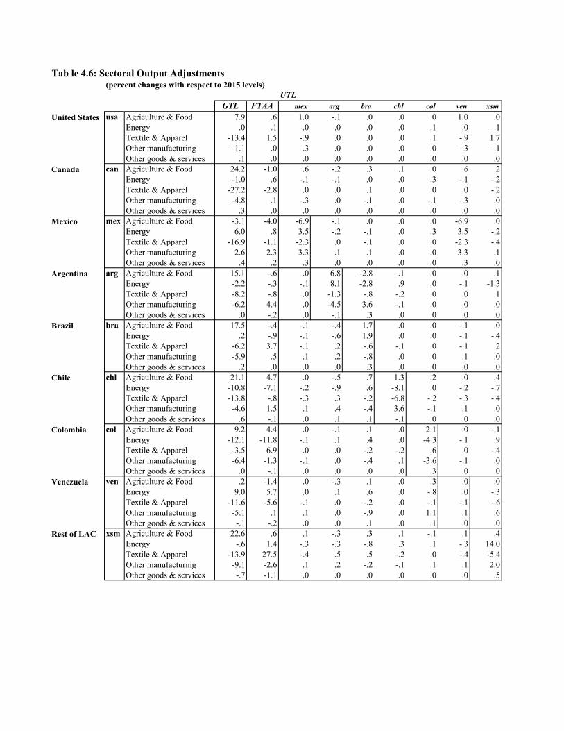
Tab le 4.6: Sectoral Output Adjustments(percent changes with respect to 2015 levels)
UTLGTL FTAA mex arg bra chl col ven xsm
United States usa Agriculture & Food 7.9 .6 1.0 -.1 .0 .0 .0 1.0 .0Energy .0 -.1 .0 .0 .0 .0 .1 .0 -.1Textile & Apparel -13.4 1.5 -.9 .0 .0 .0 .1 -.9 1.7Other manufacturing -1.1 .0 -.3 .0 .0 .0 .0 -.3 -.1Other goods & services .1 .0 .0 .0 .0 .0 .0 .0 .0
Canada can Agriculture & Food 24.2 -1.0 .6 -.2 .3 .1 .0 .6 .2Energy -1.0 .6 -.1 -.1 .0 .0 .3 -.1 -.2Textile & Apparel -27.2 -2.8 .0 .0 .1 .0 .0 .0 -.2Other manufacturing -4.8 .1 -.3 .0 -.1 .0 -.1 -.3 .0Other goods & services .3 .0 .0 .0 .0 .0 .0 .0 .0
Mexico mex Agriculture & Food -3.1 -4.0 -6.9 -.1 .0 .0 .0 -6.9 .0Energy 6.0 .8 3.5 -.2 -.1 .0 .3 3.5 -.2Textile & Apparel -16.9 -1.1 -2.3 .0 -.1 .0 .0 -2.3 -.4Other manufacturing 2.6 2.3 3.3 .1 .1 .0 .0 3.3 .1Other goods & services .4 .2 .3 .0 .0 .0 .0 .3 .0
Argentina arg Agriculture & Food 15.1 -.6 .0 6.8 -2.8 .1 .0 .0 .1Energy -2.2 -.3 -.1 8.1 -2.8 .9 .0 -.1 -1.3Textile & Apparel -8.2 -.8 .0 -1.3 -.8 -.2 .0 .0 .1Other manufacturing -6.2 4.4 .0 -4.5 3.6 -.1 .0 .0 .0Other goods & services .0 -.2 .0 -.1 .3 .0 .0 .0 .0
Brazil bra Agriculture & Food 17.5 -.4 -.1 -.4 1.7 .0 .0 -.1 .0Energy .2 -.9 -.1 -.6 1.9 .0 .0 -.1 -.4Textile & Apparel -6.2 3.7 -.1 .2 -.6 -.1 .0 -.1 .2Other manufacturing -5.9 .5 .1 .2 -.8 .0 .0 .1 .0Other goods & services .2 .0 .0 .0 .3 .0 .0 .0 .0
Chile chl Agriculture & Food 21.1 4.7 .0 -.5 .7 1.3 .2 .0 .4Energy -10.8 -7.1 -.2 -.9 .6 -8.1 .0 -.2 -.7Textile & Apparel -13.8 -.8 -.3 .3 -.2 -6.8 -.2 -.3 -.4Other manufacturing -4.6 1.5 .1 .4 -.4 3.6 -.1 .1 .0Other goods & services .6 -.1 .0 .1 .1 -.1 .0 .0 .0
Colombia col Agriculture & Food 9.2 4.4 .0 -.1 .1 .0 2.1 .0 -.1Energy -12.1 -11.8 -.1 .1 .4 .0 -4.3 -.1 .9Textile & Apparel -3.5 6.9 .0 .0 -.2 -.2 .6 .0 -.4Other manufacturing -6.4 -1.3 -.1 .0 -.4 .1 -3.6 -.1 .0Other goods & services .0 -.1 .0 .0 .0 .0 .3 .0 .0
Venezuela ven Agriculture & Food .2 -1.4 .0 -.3 .1 .0 .3 .0 .0Energy 9.0 5.7 .0 .1 .6 .0 -.8 .0 -.3Textile & Apparel -11.6 -5.6 -.1 .0 -.2 .0 -.1 -.1 -.6Other manufacturing -5.1 .1 .1 .0 -.9 .0 1.1 .1 .6Other goods & services -.1 -.2 .0 .0 .1 .0 .1 .0 .0
Rest of LAC xsm Agriculture & Food 22.6 .6 .1 -.3 .3 .1 -.1 .1 .4Energy -.6 1.4 -.3 -.3 -.8 .3 .1 -.3 14.0Textile & Apparel -13.9 27.5 -.4 .5 .5 -.2 .0 -.4 -5.4Other manufacturing -9.1 -2.6 .1 .2 -.2 -.1 .1 .1 2.0Other goods & services -.7 -1.1 .0 .0 .0 .0 .0 .0 .5

10/28/2001 33 DRAFT – Do Not Quote
The lack of structural congruence is more dramatic among other FTAA members.
Canada has two sectors moving in the same direction, two in sharply and one in
moderately opposing directions. Mexico exhibits the highest congruence of the group,
with complete qualitative agreement and surprisingly homogeneous quantitative shifts.
Argentina would experience a reversal of fortune in Agriculture and Food by moving
from FTAA to GTL, with a small contraction leading to a large (15.1%) expansion of real
output. Adjustments in Brazil are diametrically opposed between the FTAA and GTL,
with large opposing shifts in four of five aggregate sectors. Chile, Colombia, and
Venezuela all show higher levels of FTAA-GTL congruence, with notable exceptions.
The latter include Textiles and Apparel in Colombia, which would expand under FTAA
but contract under GTL. The same reversal would be even more dramatic for Rest of
LAC. These results particularly reinforce the perception of regionalism as de facto
discriminatory mechanism, effecting trade diversion incompatible with extension to
global free trade. Clearly, Textiles and Apparel in Brazil, Colombia, and Rest of LAC are
benefiting from a competitive disadvantage that FTAA confers on Asian exporters.
Comparison with the UTL results is instructive for a variety of reasons. Firstly,
we can compare the congruence of UTL with the GTL and FTAA regimes to better
interpret incentive properties. The greater the structural congruence, the easier it might be
to transition from most expedient unilateralism to eventual globalization. It can also be
argued that congruence between UTL and FTAA confers a first-mover advantage on the
country in question. The underlying political economy of adjustment being similar, they
can implement UTL and realize its gains quickly, making the transition to FTAA without
too much more structural or political adjustment. Unfortunately, there are no general
tendencies apparent in these results to support either reasoning. In some cases (Mexico,
Chile, Colombia), UTL is fairly congruent with FTAA, while in some (Mexico and
Brazil) it is more congruent with GTL. Only Mexico has high congruence across all three
regimes, but in most cases unilateralism would be a false start toward regionalism,
globalization, or both.

10/28/2001 34 DRAFT – Do Not Quote
4.4. Endogenous Productivity Growth
One final issue we want to address in these scenarios is that of endogenous
productivity growth. It has been strenuously argued in recent years that one of the
primary benefits of greater outward orientation is the internalization of factors, practices,
and processes that embody every higher productivity standards. These can be infused into
domestic economic activities through a myriad of channels, including foreign partnership,
technology transfer, access to foreign education and institutions, and even policy reform
conferred by official bilateral and multilateral ties. Whatever the mechanisms, most are
thought to affect domestic productivity in a way that is positively correlated with
economic openness.
To assess the empirical significance of these influences, we have incorporated
endogenous productivity growth in our model and recast the GTL and FTAA scenarios
using median case estimates of the relevant structural parameters.22 The results are
summarized for aggregate welfare in Table 4.7. As one might reasonably expect, the real
gains from liberalization can be significantly greater, but the make much more difference
in the transition to globalization than to the outcome of FTAA. The reason for this is
primarily the scope of trade expansion, which is over four times greater under GTL (see
Table 4.1). It should be noted that some countries (Brazil, Colombia, and Venezuela)
attain a much larger percentage of their GTL gains, under FTAA, with productivity
growth than without it. This is because the productivity boost is greatest for countries
removing the most prior protection.
22 This specification is discussed more detail in the appendix.

Table 4.7: Equivalent Variation Effects - Endogenous Productivity (percent of 2015 baseline income)
GTL FTAANeutral P-shock Neutral P-shock
United States usa .2 .5 .1 .1Canada can .3 .4 .1 .1Mexico mex .1 .5 .4 .5Argentina arg 1.2 2.0 .6 1.9Brazil bra 1.6 3.1 .5 1.5Chile chl .6 .8 .1 .2Colombia col .2 1.0 .1 .7Venezuela ven 1.5 2.0 1.2 1.6Rest of LAC xsm 1.9 2.3 1.0 1.3Western Europe eur .8 1.2 .0 .0Rest of hi-income jpn .8 1.5 .0 .0Japan rhy 2.3 2.1 -.1 .0China chn 1.1 5.3 -.1 -.1Rest of East Asia xea 2.8 3.7 -.1 -.1South Asia sas .5 3.1 -.1 .0Rest of the World row 1.0 2.4 .0 .0High-income countries hiy .4 .7 .1 .3Low- and mid-income liy 1.1 2.1 .0 .0World total wlt .8 1.6 .0 .1LAC Only lac 1.1 2.0 .0 .0DCs Excluding LAC lix .9 2.3 .0 .0
10/28/2001 36 DRAFT – Do Not Quote
5. Conclusions and Extensions
In this paper, we use a global empirical simulation model to examine a variety of
trade liberalization scenarios for the Americas. In particular, we compare global trade
liberalization (GTL) that abolishes all tariffs, regional tariff liberalization (RTL) that
eliminates tariffs within the Americas and Caribbean, and unilateral trade liberalization
(UTL) by selected Latin American countries. Our results are consistent with some
conventional intuition, but in other ways contradict conclusions obtained from simplified
theoretical models. For example, we find that GTL yields the greatest benefit, both for
the rest of the world and for RTL members, while an FTAA arrangement is beneficial to
all members, expands intra-regional trade fivefold, but induces significant trade diversion
away from nonmembers. Despite the fact that GTL gains are many times those of the
RTL for members, one might still expect to see the latter negotiated because of
uncertainties about realization of GTL and because members may not see the RTL and
GTL as mutually exclusive.
Our results do not support the theoretical suggestion, around since the 1950’s, that
unilateralism generally dominates RTL membership, or its corollary that prospective
members must be induced to join by incentives written into the RTL agreement. Indeed,
in most cases we study, prospective members gain significantly less from UTL and would
probably experience structural reversals by pursuing this as a first move toward RTL
participation, thus reducing the net benefit of the latter. The only UTL that generally
dominates RTL is one where each of the country’s trading partners reciprocates by
eliminating (only) bilateral tariffs. Not only is this a very implausible scenario, but such
benefits do not aggregate into anything representing a larger regional agreement,
reflecting none other than the fallacy of composition.
We also examine the issue of structural congruence between the three levels of
trade liberalization, meaning the extent to which different policies induce harmonious
shifts in output structure. Our findings indicate that, for most countries, GLT, RTL, and
UTL induce resource pulls and shifts in output composition in significantly different
directions. This implies that, in a hypothetical transition from UTL to RTL to GTL (or
any pair wise transition), output in many sectors would reverse themselves and

10/28/2001 37 DRAFT – Do Not Quote
sometimes significantly so. This in turn would give rise to very different regimes of
political economy, depending on the beginning and ending policy scenarios. Thus, for
example, it may not be reasonable to see the FTAA as a milestone on the way to GTL,
apart from general learning and institution building in the domains of multilateralism
generally and trade negotiation in particular.
The most salient lesson from this preliminary work, however, may be the essential
role that detailed empirical analysis can play in support of strategic trade policy. It is
obvious from the complexity of influences giving rise to our results that policy makers
relying on economic theory, intuition, or rules of thumb alone are unlikely to adequately
foresee the consequences of their actions. Not only are the magnitudes of induced
adjustments difficult to ascertain because of the scope of indirect effects, but qualitative
outcomes often directly contradict intuition or the predictions of highly simplified
models, leading to the opposite results from the intended ones. Fortunately, models and
data of the kind used here are now well established research tools. They can now be
applied to a large universe of issues to better elucidate the economic consequences of
policy before it is implemented.

10/28/2001 38 DRAFT – Do Not Quote
6. References Anderson, Kym, Joe Francois, Tom Hertel, Bernard Hoekman and Will Martin (2000), “Potential
gains from trade reform in the new millennium,” Paper presented at the Third Annual Conference on Global Economic Analysis, held at Monash University, 27-30 June. (Available at http://www.monash.edu.au/policy/conf/65Anderson.pdf )
Armington, Paul (1969), “A Theory of Demand for Products Distinguished by Place of Production,” IMF Staff Papers, Vol. 16, pp. 159-178.
Brown, Drusilla K., Alan V. Deardorff and Robert M. Stern (1992), “A North American Free Trade Agreement: Analytical Issues and a Computational Assessment” The World Economy, 15, pp. 15-29. (See also http://www.spp.umich.edu/rsie/model/analytics.html for model specification )
Brown, Drusilla K., Alan V. Deardorff and Robert M. Stern (2001), “CGE Modeling and Analysis of Multilateral and Regional Negotiating Options,” Research Seminar in International Economics Discussion Paper, No. 468, School of Public Policy, The University of Michigan, Ann Arbor. (Available at http://www.spp.umich.edu/rsie/workingpapers/papers451-475/r468.pdf )
Burniaux, Jean-Marc, and Dominique van der Mensbrugghe (1994), “The RUNS Global Trade Model,” Economic & Financial Modelling, Autumn/Winter, pp. 161-282.
Burniaux, Jean-Marc, Giuseppe Nicoletti and Joaquim Oliveira-Martins (1993), “GREEN: A Global Model for Quantifying the Costs of Policies to Curb CO2 Emissions,” OECD Economic Studies: Special Issue on The Economic Costs of Reducing CO2 Emissions, No. 19, Winter 1992, pp. 49-92.
Collado, Juan Carlos, David Roland-Holst and Dominique van der Mensbrugghe (1995), “Latin America Employment Prospects in a More Liberal Trading Environment,” in Social Tensions, Job Creation and Economic Policy in Latin America, David Turnham, Colm Foy and Guillermo Larrain, editors, OECD, Paris.
de Melo, Jaime, and Sherman Robinson (1989), “Product Differentiation and the Treatment of Foreign Trade in Computable General Equilibrium Models of Small Economies,” Journal of International Economics, Vol. 27, pp. 47-67.
Deaton, Angus, and John Muellbauer (1980), Economics and Consumer Behaviour, Cambridge University Press, Cambridge, UK.
Derviş, Kemal, Jaime de Melo and Sherman Robinson (1982), General equilibrium models for development policy, A World Bank Research Publication, Cambridge University Press, New York, NY.
Dessus, Sébastien, Kiichiro Fukasaku and Raed Safadi (1999), “Multilateral Tariff Liberalisation and the Developing Countries,” OECD Development Centre Policy Brief, No. 18, Paris. (Available at http://www.oecd.org/dev/ENGLISH/publication/Policy-B/pb18a.pdf )
10/28/2001 39 DRAFT – Do Not Quote
Francois, Joseph and Kenneth Reinert (1997), Applied Methods for Trade Policy Analysis : A Handbook, Cambridge University Press, New York, NY.
Francois, Joseph F., Bradley McDonald and Häkan Nordström (1996), “The Uruguay Round: a numerically based qualitative assessment,” in W. Martin and L. A. Winters, ed., The Uruguay Round and the developing countries, Cambridge University Press, Cambridge, UK.
Fullerton, Don (1983), “Transition Losses of Partially Mobile Industry-specific Capital,” Quarterly Journal of Economics, Vol. 98, February, pp. 107-125.
Goldin, Ian, Odin Knudsen and Dominique van der Mensbrugghe (1993), Trade Liberalization: Global Economic Implications, OECD/The World Bank, Paris.
Harrison, Glenn W., Thomas F. Rutherford and David Tarr (1996), “Quantifying the Uruguay Round,” in W. Martin and L. A. Winters, ed., The Uruguay Round and the developing countries, Cambridge University Press, Cambridge, UK.
Hertel, Thomas W., editor (1997), Global Trade Analysis: Modeling and Applications, Cambridge University Press, New York, NY.
Hoekman, B and M. Kostecki (1995), The Political Economy of the World Trading System: From GATT to WTO, New York/Oxford, Oxford University Press.
Hoekman, B. and Leidy (1993), “Holes and Loopholes in Regional Integration Agreements,” in K. Anderson and R. Blackhurst (eds.), Regional Integration. London: Harvester-Wheatsheaf.Howe, Howard (1975), “Development of the Extended Linear Expenditure System from Simple Savings Assumptions,” European Economic Review, Vol. 6, pp. 305-310.
Ianchovichina, Elena, and Robert McDougall (2000), “Theoretical Structure of Dynamic GTAP,” GTAP Technical Paper, No. 17, Center for Global Trade Analysis, Department of Agricultural Economics, Purdue University. (Available at http://www.agecon.purdue.edu/gtap/resources/download/160.pdf )
Kemp, M.C. and H.Y. Wan (1976) “An Elementary Proposition Concerning the Formation of Customs Unions,” in M.C. Kemp, Three Topics in the Theory of International Trade, Amsterdam: North Holland.
Lawrence, Robert Z. (1996), Regionalism, Multilateralism and Deeper Integration. Washington DC: Brookings Institution.
Lee, Hiro, David Roland-Holst and Dominique van der Mensbrugghe (1999), “APEC Trade Liberalization and Structural Adjustment: Policy Assumptions,” APEC Discussion Paper Series, APEC Study Center, Graduate School of International Development, Nagoya University, March.
Lluch, Constantino (1973), “The Extended Linear Expenditure System,” European Economic Review, Vol. 4, pp. 21-32.
10/28/2001 40 DRAFT – Do Not Quote
Maechler, A.M. and David Roland-Holst (1997), “Labor Market Specification for Empirical General Equilibrium Analysis,” in J.F. Francois and K.A. Reinert (eds.), op. cit.
Martin, Will, and L. Alan Winters, editors (1996), The Uruguay Round and the developing countries, Cambridge University Press, Cambridge, UK.
Melo, J. de, A. Panagariya, and D. Rodrik (1993) “The New Regionalism: A Country Perspective,” in Melo, J. de and A. Panagariya (eds.), New Dimensions in Regional Integration, London: Centre for Economic Policy Research and Cambridge UP.
OECD (1990), OECD Economic Studies: Special Issue on Modelling the Effects of Agricultural Policies, No. 13, Winter 1989/90, Paris.
OECD (1998), “Economic Modelling of Climate Change,” OECD Workshop Report, 17-18 September, 1998, Paris. (Summary available at http://www.oecd.org/dev/news/Environment/summary.pdf )
Reinert, K.W., Ricuarte, M., and D. Roland-Holst (1998), “Qué diferencia un país? Efectos de los loops abiertos y cerrados en la América del Norte,” El Trimestre Económico, Vol. LXV (4), Núm. 260, 505-518,1998.
Rutherford, Thomas F., and David G. Tarr (2001), “Trade liberalization, product variety and growth in a small open economy: a quantitative assessment,” Journal of International Economics, forthcoming.
van der Mensbrugghe, Dominique (1994), “GREEN: The Reference Manual”, OECD Economics Department Working Papers, No. 143, OECD, Paris.
van der Mensbrugghe, Dominique (1998), “Trade, Employment and Wages: What Impact from 20 More Years of Rapid Asian Growth?” in The Future of Asia in the World Economy, Colm Foy, Francis Harrigan, and David O’Connor, editors, OECD, Paris.
van der Mensbrugghe, Dominique (2001), “LINKAGE Technical Reference Document,” Economic Policy and Prospects Group, The World Bank, Processed, October. (Available at http://www.worldbank.org/prospects/pubs/TechRef.pdf ),
van der Mensbrugghe, Dominique, and Ramiro Guerrero (1998), “Free Trade Arrangements in the Americas: Quid for Agriculture?” paper presented at a joint IPEA/IDB conference on FTAA and MERCOSUR: The Brazilian Economy and the Process of Regional and Subregional Integration, Brasilia, 5-6 October.
Viner, J. (1950), The Customs Union Issue, New York: Carnegie Endowment for International Peace.
Whalley, John (1996), “Why Do Countries Seek Regional Trade Agreements?”, Chapter 3 in Frankel, J. (ed.) The Regionalization of the World Economy, Chicago, Chicago UP.
World Bank. (2000). Trade Blocs. Policy Research Report. World Bank/Oxford UP.
World Bank (2000), From Natural Resources to the Knowledge Economy: Trade and Job Quality. Policy Research Report, World Bank, processed, 229pp.

10/28/2001 41 DRAFT – Do Not Quote
7. Appendix
7.1. Equivalent Variation Aggregate National Income
Aggregate income gains and/or losses summarize the extent trade distortions are
hindering growth prospects and the ability of economies to use the gains to help those
whose income could potentially decline.
Real income is summarized by Hicksian equivalent variation (EV). This
represents the income consumers would be willing to forego to achieve post-reform well-
being (up) compared to baseline well-being (ub) at baseline prices (pb):
( ) ( )bbpb upEupEEV ,, −=
where E represents the expenditure function to achieve utility level u given a vector of
prices p (the b superscript represents baseline levels, and p the post-reform levels). The
model uses the extended linear expenditure system (ELES), which incorporates savings
in the consumer’s utility function. See Lluch (1973) and Howe (1975). The ELES
expenditure function is easy to evaluate at each point in time. (Unlike the OECD
treatment of EV, we use baseline prices in each year rather than base year prices. See
Burniaux et al. (1993)). The discounted real income uses the following formula:
( ) ( )∑∑=
−
=
−=2015
2005
20042015
2005
2004 /t
dt
t
t
at
t YEVCEV ββ
where CEV is the cumulative measure of real income (as a percent of baseline income), β
is the discount factor (equal to 1/(1+r) where r is the subjective discount rate), Yd is real
disposable income, and EVa is adjusted equivalent variation. The adjustment to EV
extracts the component measuring the contribution of household saving, since this
represents future consumption. Without the adjustment, the EV measure would be double
counting. The saving component is included in the EV evaluation for the terminal year.
Similar to the OECD, a subjective discount rate of 1.5 percent is assumed in the
cumulative expressions.

10/28/2001 42 DRAFT – Do Not Quote
7.2. Specification of Endogenous Productivity Growth
Productivity in manufacturing and services is the sum of three components:
• a uniform factor used as an instrument to target GDP growth in the
baseline simulation
• a sector-specific fixed shifter which allows for relative differentials across
sectors (for example, manufacturing productivity two percentage points
higher than productivity in the services sectors)
• a component linked to sectoral openness as measured by the export-to-
output ratio
The latter takes the following functional form:
(1) η
χγ
=
i
ii
ei X
E0
where γe is the growth in sectoral productivity due to the change in openness, χ0 is a
calibrated parameter, E and X represent respectively sectoral export and output, and η is
the elasticity. The parameter χ0 has been calibrated so that (on average) openness
determines roughly 40 percent of productivity growth in the baseline simulation, and the
elasticity has been set to 1.
In agriculture, productivity is fixed in the baseline, set to 2.5 percent per annum in
most developing countries (based on estimates found in Martin and Mitra, 19xx).
However, a share of the fixed productivity is attributed to openness, using equation (1).
In the baseline, GDP growth is given. Agricultural productivity is similarly given,
and equation (1) is simply used to calibrate the shift parameter, χ0, so that a share of
agricultural productivity is determined by sectoral openness. Average productivity in the
manufacturing and services sectors is endogenous and is calibrated in the baseline to
achieve the given GDP growth target. The economy-wide (excluding agriculture)
productivity parameter is endogenous. Equation (1) is used to calibrate the same χ0

10/28/2001 43 DRAFT – Do Not Quote
parameter, under the assumption that some share of sectoral productivity is determined
by openness, for example 40 percent.
In policy simulations, the economy-wide productivity factor, along with other
exogenous productivity factors (sector-specific shifters) are held fixed, but the openness-
related part of productivity is endogenous and responds to changes in the sectoral export-
to-output ratio. In the manufacturing and services sectors, the elasticity is set at 1. In the
agricultural sectors it is set to 0.5.
Say sectoral productivity is 2.5 percent, and that 40 percent of it can be explained
by openness, i.e. 1.0 percent, with the residual 1.5 percent explained by other factors.
Assume sectoral openness increases by 10 percent. If the elasticity is 1, this implies that
the openness-related productivity component will increase to 1.1 percent and total
sectoral productivity will increase to 2.6 percent (implying that the total sectoral
productivity increases by 4 percent with respect to the 10 percent increase in sectoral
openness).
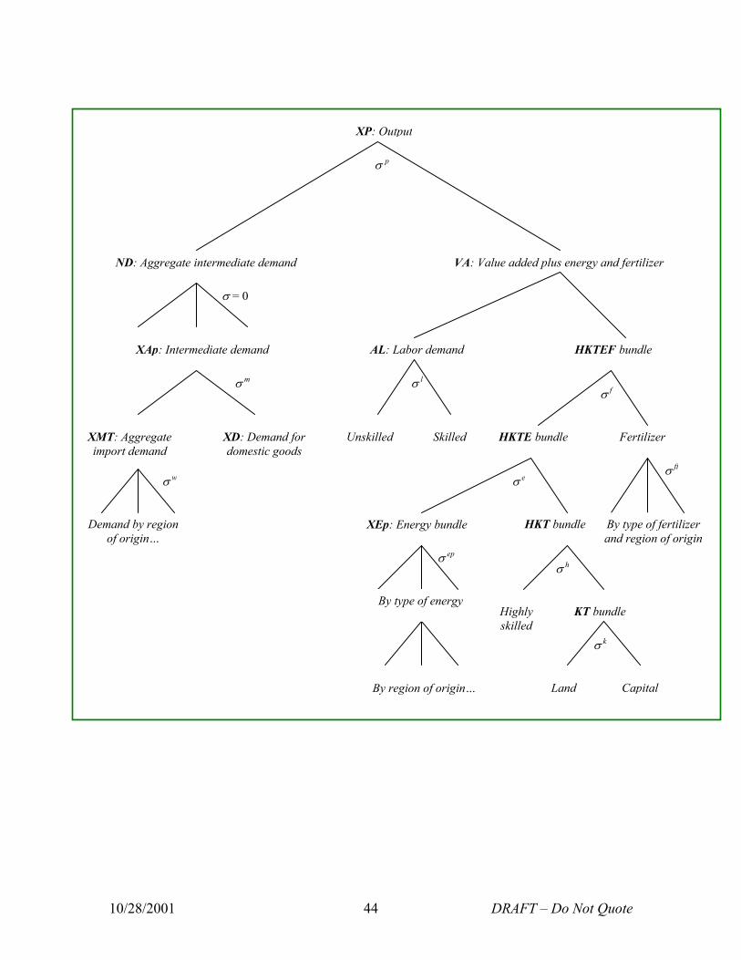
10/28/2001 44 DRAFT – Do Not Quote
σ p
Highly skilled
KT bundle
Land Capital
σ = 0
σ m
σ w
σ ep
σ k
σ h
σ l
σ e σ ft
σ f
HKT bundle
VA: Value added plus energy and fertilizer
XMT: Aggregate import demand
ND: Aggregate intermediate demand
XP: Output
XAp: Intermediate demand
Demand by region of origin…
XD: Demand for domestic goods
AL: Labor demand
Unskilled Skilled
HKTEF bundle
HKTE bundle Fertilizer
By type of fertilizer and region of origin
XEp: Energy bundle
By type of energy
By region of origin…

10/28/2001 45 DRAFT – Do Not Quote
σ = 0
σ ep
σ h
σ fd
σ f
σ eσ l
σ v
σ w
σ m
Feed AL: Labor demand
XMT: Aggregate import demand
XP: Output
ND: Aggregate intermediate demand
XAp: Intermediate demand
XD: Demand for domestic goods
WTF: Demand by region of origin
VA: Value added plus energy and feed
TFD: Land and feed bundleKTEL bundle
HKTE bundle
XEp: Energy bundle
HKT bundle
Unskilled Skilled
Energy demand by type of energy and
region of origin
Feed demand by type of feed and region of origin
Capital Highly skilled
Land
σ p
σ = 0

10/28/2001 46 DRAFT – Do Not Quote
XP: Output
ND: Aggregate intermediate demand VA: Value added plus energy
XAp: Intermediate demand
XD: Demand for domestic goods
XMT: Aggregate import demand
WTF: Demand by region of origin
AL: Labor demand
Unkilled Skilled
HKTE bundle
HKT bundleXEp: Energy bundle
KT bundle Highly skilled
By type of energy
By region of origin…
σ p
Sector-specific factor
σ v
σ e
σ hσ ep
σ m
σ w
σ l
σ = 0
σ k
Capital

10/28/2001 47 DRAFT – Do Not Quote
XA: Armington demand
XD d: Domestic demand for domestic production
XD s: Local production supplied to domestic market
XMT: Aggregate import demand
WTF d: Import demand by region of origin
WTF s: Local production supplied by region of destination
ES: Aggregate export supply
σ m
σ w
σ x
σ z
XP: Domestic supply
Constant-elasticity-of-transformation supply
specification
Constant-elasticity-of-substitution demand
specification