15

Regional precipitation climates of Iran

Reza ModarresIsfahan University of Technology, Isfahan, Iran

Journal of Hydrology (NZ) 45 (1): 15-, 2006© New Zealand Hydrological Society (2006)

AbstractRainfall in Iran is complex, with unpredict­able fluctuations from year to year and from region to region. At­site frequency analysis is inadequate for regional planning. Thus, it is important to determine regional rainfall frequencies. Hierarchical cluster analysis and L­moments regional frequency analysis were used in this study to find homogeneous rainfall groups and regional rainfall frequency distributions. The study showed eight homogeneous rainfall regions within Iran, which correspond with areas with differing geography and climate. A regional homogeneity measure, H1, showed that a 3­parameter log­normal distribution describes the overall distribution of rainfall within Iran, but because of substantial variations in precipitation patterns within the country, the distribution is not applicable for individual regions. Z­statistics, which are based on L­moments, were used to select the distribution that best fitted rainfall records in each homogeneous region.

Key WordsRainfall frequency analysis, cluster analysis, Ward’s method, L­moments, Iran

IntroductionRainfall frequency analysis is important for atmospheric research, flood estimation models and hydrologic design, planning and management. Rainfall variation within

Iran is complex, with unpredictable rainfall fluctuations from year to year and from region to region. To simplify hydrologic calculations and reduce masses of observa­tions and variables for frequency analysis, meteorologists and hydrologists have tried to group spatial and temporal patterns to define homogenous rainfall regions within Iran.

Several methods are commonly used for the regionalization of hydrologic phenomena such as rainfall, streamflow and other components of the water cycle, to determine if an area has hydrologically homogeneous regions. Multivariate techniques can be powerful tools for classifying meteorological data such as rainfall. Principle component analysis, factor analysis and different types of cluster analysis have been used to classify daily rainfall patterns and their relationship to atmospheric circulation (Romero et al., 1999), flood and drought years (Singh, 1999), and streamflow drought (Stahl and Demuth, 1999). Gottschalk (1985) suggested the application of multivariate methods to classify hydrologic events on a national scale. Guttman (1993) applied L­moments and cluster analysis to determine regional rainfall climates within conterminous United States; he defined 104 homogeneous precipitation regions there.

One of the first efforts on rainfall regional­ization in Iran was carried out by Vaziri (1997), who divided Iran into seven groups based on rainfall intensity­duration curves. Recently, Masoodian (1998) and Domroes et al. (1998) have applied multivariate principle

16

component techniques to classify rainfall patterns in Iran; they found six and five precipitation groups across Iran, respectively.

This study examines rainfall frequency distributions in Iran to find regional patterns. Because of the variation of rainfall pattern, we first classify rainfall spatial groups in Iran through cluster analysis, and then apply L­moment procedures for regional frequency analysis within the homogeneous areas defined by the cluster analysis.

Rainfall dataThe annual and monthly rainfall of 28 main cities of the provinces of Iran are used as the data set to determine Iran’s rainfall spatial patterns. The World Meteorological Organization (WMO) suggests using 30­year rainfall periods for rainfall analysis, but when analysing variations over time, data for shorter periods (10 or 20 years) can also be used (Moron, 1997; Salinger and Mullan, 1999; Ramos, 2001). The data set

of this study contains annual and monthly rainfalls with record lengths ranging from 13 to 30 years. Masoodian (1998) showed that the average annual rainfall of Iran is 260 mm, with a maximum rainfall along the margin of the Caspian Sea in the north of Iran: the main city of Guilan province, Rasht, is representative of this region. Figure 1 shows the spatial distribution of the stations in Iran used in this study. The boundary of each province is also illustrated.

Cluster analysisCluster analysis for hydrologic regionalization involves the grouping of observations or variables into clusters, with each cluster containing observations or variables with highly similar hydrologic characteristics, such as geographical, physical, statistical or stochastic features. Mosley (1981) used hierarchical clusters for the rivers in New Zealand and Tasker (1982) compared methods of defining homogeneous regions, including

Figure 1 – Provinces of Iran and the location of the selected rainfall stations in each province.

17

cluster analysis, with a complete linkage algorithm. Acreman (1985) and Acreman and Sinclair (1986) concluded that cluster analysis is useful for explaining observed variation in their data. Gottschalk (1985) applied cluster and principal component analysis to data from Sweden and found that cluster analysis is suitable to use on a national scale for a country with heterogeneous hydrological regimes. Nathan and McMahon (1990) used hierarchical cluster analysis to predict low­flow characteristics in southeastern Australia. They found that Ward’s method, with a dissimilarity measure based on the squared Euclidean distance, is the best method for classification.

The commonly used dissimilarity Euclidean distance measure is written as follows:

drs2 = (xrj – xsj )

2

j=1

p

∑ (1)

where rth and sth rows of the data matrix, X, are denoted by (xr1, xr2, …,xrp) and (xs1, xs2, …, xsp) respectively. These two rows correspond to the observations on two objects for all P variables. The quantity drs

2 is referred to as the squared Euclidean distance (Jobson, 1992). The Euclidean distance of dissimilarity is then used in the cluster techniques.

In this study, we apply the hierarchical cluster technique described by Kaufman and Rousseuw (1990). Several methods have been proposed for hierarchical cluster analysis, including single, average and complete linkage, and Ward’s minimum variance method; both average linkage and Ward’s method are widely used (Milligan, 1980; Jackson and Weinand, 1995; Ramos, 2001). Nathan and McMahon (1990), Masoodian (1998) and Domroes et al. (1998) indicate that Ward’s method gives better results, so we have used Ward’s method for cluster analysis of rainfall data in this study.

Ward’s method calculates the distance between two clusters as the sum of squares between two clusters, added up over all variables. At each generation, the sum of squares is minimized. If CK and CL are two rainfall clusters that merged to form the cluster CM, the distance between the new cluster and another cluster CJ is:

dJ.M =((nJ + nK ))djk + (nJ + nL )dJL – nJdKL )

nJ + nM (2)

where nJ, nK, nL and nM are the number of the rainfall stations in clusters J, K, L and M, respectively, and dJK, dJL and dKL represent the distances between the rainfall observations in the clusters J and K, J and L, and K and L, respectively. To select a suitable number of rainfall clusters, two statistics are used: pseudo F and t 2 statistics (SAS,1999) (not shown here).

Based on the Ward’s method and using the annual and monthly rainfall (1+12 variables) of the selected rainfall stations, eight clusters can be found, based on the greatest similarity (smallest dissimilarity):1) Yazd, Zahedan, Isfahan, Semnan, Kerman

and Ghom;2) Arak, Shahrecord, Ghazvin, Tehran,

Mashhad and Hameda;3) Oroomieh, Ardabil, Zanjan and Tabriz;4) Ahwaz, Bushehr, Shiraz, and with a small

difference, Bandarabbas;5) Kermanshah, Sanandaj and Khoramabad;6) Ghaemshahr and Gorgan;7) Ilam and Yasuj;8) Rasht.

These eight clusters cover 90 per cent of the rainfall variance within Iran. The first group is the largest: it includes stations in arid and semi­arid regions in the centre of Iran. The second group is stations located in the highland margins of regions in the first group. Another group includes stations in the northwestern cold region – Oroomieh, Ardabil, Zanjan and Tabriz stations (called

18

the ‘Azari’ group by Masoodian (1998)). The fourth group includes stations along the margin of the Persian Gulf in the south of Iran, while the sixth and the eighth groups are areas located along the margin of the Caspian Sea. The major difference between the sixth and eighth groups in the north of Iran is the amount of rainfall, which decreases from west (Rasht) to east (Ghaemshahr and Gorgan). The fifth and seventh groups are regions in the Zagros Mountains, with the amount of rainfall higher in the seventh group. The geographic distribution of the eight groups is shown in Figure 2. Once these cluster­ based groups were distinguished, we applied L­moments to check the homogeneity of each group and to find the regional frequency distribution for each one.

Regional frequency analysisHydrologists have proposed several methods for regional frequency analysis. Perhaps the most popular method is L­moments.

Figure 2 – Spatial distribution of rainfall groups over Iran.

Greenwood et al. (1979) introduced the concept of probability­weighted moments. Hosking (1990) defined L­moments as equivalent to probability­weighted moments, as L­moments can be expressed by linear combinations of probability­weighted moments (Rao and Hamed, 1997). Hosking and Wallis (1993) extended the use of L­moments and developed useful statistics for regional frequency analysis to measure discordancy, regional homogeneity and goodness of fit.

Homogeneity and discordancy testHosking and Wallis (1993) derived two statistics to test the homogeneity of a region. The first statistic (Hi, i=1, 2 and 3) is used as a measure of homogeneity. A region is homogenous if Hi is less than 1, possibly heterogeneous if Hi is between 1 and 2, and definitely heterogeneous if Hi is greater than 2 (Hosking and Wallis, 1993). In this study,

19

we use H1 to measure regional homogeneity, as suggested by Rao and Hamed (1997). H1 is more effective in determining homogenous regions than H2 and H3. H1 is based on L­Cv only. Using the FORTRAN computer program developed by Hosking (1991), the homogeneity measure for all 28 stations is H1=8.43. Based on this statistic, rainfall across Iran is definitely heterogeneous, because of large geographic and climatic differences within the country.

The second statistic is used as a measure of discordancy. If the discordancy measure (D) is larger than 3, the site is considered to be discordant. The results of discordancy analysis for all the stations are presented in Table 1. Only Yazd station has a value of (D) greater than 3. We then calculated the homogeneity measure for each group derived from the cluster analysis to see if these groups are homogenous. Table 2 summarises the homogeneity measures of each group.

Table 1 – Descriptive and L­moments statistics of the rainfall at selected stations

Sample No. size Station name MEAN STDEV L-Cv L-Cs L-Ck D

1 30 Ahwaz 213.30 86.30 0.18 ­0.13 0.07 0.56 2 30 Arak 345.00 92.78 0.15 ­0.28 ­0.09 1.72 3 23 Ardabil 309.00 88.02 0.15 ­0.13 ­0.07 0.91 4 30 Bandarabbas 192.00 121.80 0.31 0.04 0.03 2.75 5 30 Bushehr 275.60 118.81 0.22 0.04 0.05 0.52 6 30 Ghaemshahr 752.30 116.68 0.08 ­0.28 ­0.01 1.33 7 25 Gorgan 612.10 102.83 0.09 ­0.39 ­0.01 0.78 8 30 Ghazvin 315.90 89.48 0.15 ­0.08 ­0.02 0.47 9 23 Hamedan 316.20 76.57 0.13 ­0.20 ­0.06 0.52 10 30 Isfahan 121.40 40.10 0.17 ­0.23 ­0.03 1.47 11 13 Ilam 627.90 170.69 0.14 ­0.44 ­0.10 0.42 12 30 Oroomieh 349.30 98.40 0.16 0.0 0.02 0.99 13 13 Ghom 149.00 47.10 0.17 ­0.41 ­0.26 1.72 14 30 Zahedan 94.80 40.14 0.26 0.11 ­0.04 1.92 15 30 Zanjan 317.60 72.60 0.13 ­0.28 0.01 0.56 16 30 Yazd 62.10 27.88 0.67 0.75 0.59 3.32 17 13 Yasuj 822.90 183.02 0.11 ­0.58 ­0.15 0.32 18 30 Tehran 229.20 63.92 0.14 ­0.18 ­0.04 0.27 19 30 Tabriz 293.30 68.05 0.14 ­0.17 ­0.06 0.44 20 30 Shiraz 344.70 99.69 0.16 ­0.25 ­0.03 0.92 21 30 Shahrecord 319.00 86.57 0.14 ­0.16 ­0.08 0.65 22 30 Semnan 139.90 54.22 0.20 ­0.06 0.03 0.16 23 30 Sanandaj 471.00 118.78 0.13 ­0.28 0.12 2.00 24 30 Rasht 1353.00 279.35 0.11 ­0.16 ­0.03 1.07 25 30 Mashhad 257.50 77.41 0.16 ­0.13 ­0.06 0.48 26 30 Khoramabad 515.10 125.61 0.12 ­0.33 0.06 1.50 27 30 Kermanshah 450.80 120.40 0.14 ­0.20 ­0.02 0.15 28 25 Kerman 158.90 50.18 0.17 ­0.13 0.02 0.07

STDEV: Standard Deviation; L-Cv: Measure of Variation; L-Cs: Measure of skewness; L-Ck: Measure of Kurtosis; D: Discordancy measure

20

Table 2 – Homogeneity measure (H1) of the derived groups (H1* shows homogeneity measure after removing discordant station)

Group 1 Group 2 Group 3 Group 4 Group 5 Group 6 Group 7

H1 1.08 ­1.65 ­0.9 2.47 ­0.96 ­0.52 ­0.53 H1* 0.06 – – 0.55 – – –

Discordant station Yazd – – Bandarabbas – – –

As group 8 has only one station, we could not calculate H statistics for this group. There are two discordant stations: Yazd in group 1 and Bandarabbas in group 4. Yazd lies the middle of the central arid zone of Iran and Bandarabbas is a harbor city next to the Persian Gulf. Their rainfall patterns are thus very different from patterns of other stations in their groups. If we remove these stations from the groups and recalculate H1 statistics, groups 1 and 4 are homogeneous. Except for groups 1 and 4, the negative values of H1 in other groups indicate less heterogeneity (more homogeneity) of the group. All stations in group 4 are affected by sea moisture, but Ahwaz and Shiraz stations are far from sea, in the highlands of the mountainous area. Similarly, for the stations in group 1, Yazd station is located in the centre of the arid region of Iran, while the other stations are within the semi­arid margin of the central arid zone.

Quantile estimation and goodness-of-fit-testsQuantile estimation is the main goal of hydrologic frequency analysis. Quantiles are estimated by applying a frequency distribution function. An easy way to find the frequency distribution is the moment ratio diagram. L­moment diagrams provide a visual comparison of the sample estimates with the population values of L­moments (Stedinger et al., 1993) and are always preferable to product moment ratio diagrams for a goodness­of­fit

test (Vogel and Fennessey, 1993). Figure 3 shows moment ratio diagrams for all selected stations and three of the most common 3­parameter distributions, namely, Generalized Extreme Value, Generalized Logistic, 3­parameter Log Normal and Pearson type 3 distributions. The figure was drawn using the FREQ program in MATLAB, developed by Rao and Hamed (2000). The discordant Yazd station shows different conditions, according to the LCv­LCs and LCs­LCk diagrams: it lies in the middle of Iran’s arid region, where rainfall variation is significantly higher than in other regions.

To find the best at­site and regional frequency distributions, we use the residual mean square error (RMSE) (Rao and Hamed, 1997) and an L­moment­based goodness­of­fit test procedure (Hosking and Wallis, 1993). The goodness­of­fit­test measure, ZDIST, (Hosking and Wallis, 1993) was calculated, using a FORTRAN computer program developed by Hosking (1991), for each homogeneous region resulting from the cluster analysis. If the absolute value of ZDIST is smaller than 1.64 ( ZDist <1.64), the goodness of a distribution is accepted. Table 3 shows the goodness­of fit­test measures, ZDIST, for the most important 3­ parameter distributions in seven groups of rainfall. For Groups 1, 3 and 4, all 3­parameter distributions are accepted. For Group 5, none of them is accepted and for groups 2, 6 and 7, some are accepted and the rest are not.

21

Figure 3 – Moment ratio diagrams of the selected stations.

Table 3 – The goodness­of­fit­test measure (ZDIST) for homogeneous rainfall groups within Iran (numbers in bold indicate distributions that are accepted).

Distributions Iran G1 G2 G3 G4 G5 G6 G7

Generalized Logistic 1.80 0.34 2.68 0.56 -0.30 ­2.30 -0.89 -1.09Generalized Extreme Value ­1.93 -0.73 0.56 -0.60 -1.50 3.89 ­1.83 ­1.723­parameter Log Normal -1.51 -0.84 0.87 -0.55 -1.35 ­3.47 ­1.7 -1.62Pearson type III ­1.81 -1.17 0.76 -0.73 -1.44 ­3.48 ­1.76 ­1.66

22

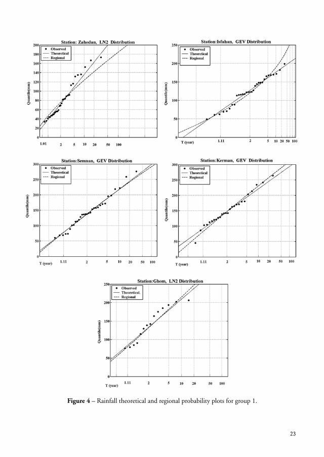
Based on the goodness­of­fit­test measure, for the entire country, a 3­parameter log normal distribution seems a better fit than the other distributions. However, because of the heterogeneity of the country, this distribution is not applicable for individual regions. For each homogeneous region, a different 3­parameter distribution can be accepted. The only reliable conclusion is that for different groups, there is no single parent distribution. This indicates substantial variation of rainfall and climate, even within each homogeneous rainfall group. The result of the at­site frequency analysis also shows this rainfall spatio­temporal dissimilarity. The best at­site frequency distribution for each station is presented in Figures 4 to 11, after removing discordant stations (Yazd and Bandarabbas).

DiscussionCluster analysisBecause of the varying spatio­temporal characteristics of rainfall across the country, a hierarchical cluster analysis was first applied to distinguish homogeneous regions. It showed that a hierarchical Ward’s method could classify the rainfall spatial pattern across the country. The derived rainfall groups and geographical conditions match each other very well, with differing rainfall clusters imply varying rainfall regimes. The central arid zone of Iran (group 1) has a high coefficient of variation and low rainfall; the cold region of northwestern Iran has a high ratio of snow to rainfall (group 3). The impact of the Zagros Mountains on rainfall is evident in western Iran (group 5), with some within­region spatial variation (group 7). Other groups encompass the lowland margins of the Caspian Sea (groups 6 and 8) and the coastal stations of the Persian Gulf, except for Shiraz station (group 4). These varying rainfall groups show that the spatial pattern of rainfall of Iran is influenced by

elevation, latitude and proximity to the sea (Masoodian, 1998; Domroes et al., 1998). This study adds several new regions to those defined by Masoodian (1998) and Domroes (1998). The present study distinguishes two regions along the margin of the Caspian Sea, while Masoodian (1998) showed only one region. Domroes et al. (1998) defined two regions in the Zagros Mountains in the west of Iran, while the present study showed that this region could be divided into at least three homogeneous regions.

Frequency AnalysisThe homogeneity measure showed that a 3­parameter log normal distribution can describe the overall rainfall distribution within Iran, but because of substantial variations in rainfall patterns, it is better to apply regional frequency analysis to individ­ual homogeneous rainfall groups. However, the results showed that we cannot select a single parent distribution for each group. The regional rainfall frequency analysis indicated that different distributions can represent the different climate characteristics of rainfall groups within Iran. The Generalised Extreme Value (GEV) distribution fits the rainfall of the very high mountain stations of group 7, a region with varied mechanisms for generating rainfall, but a 2­parameter log normal (LN2) distribution fits to the high mountain stations of group 5, where there is more uniformity in rainfall generation.

A GEV distribution also fits the Persian Gulf margin and the central arid zone of Iran, which has high rainfall variation. On the other hand, the 2­parameter log normal (LN2) distribution is a better fit for rainfall in the flat humid margin of the Caspian Sea. Different at­site frequency distributions in group 2 also suggest more complex rainfall­generating mechanisms, resulting in different rainfall spatio­temporal patterns. At­site frequency analysis also indicates that frequency distributions match the rainfall

23

Figure 4 – Rainfall theoretical and regional probability plots for group 1.

24

Figure 5 – Rainfall theoretical and regional probability plots for group 2.

25

Figure 6 – Rainfall theoretical and regional probability plots for group 3.

26

Figure 7 – Rainfall theoretical and regional probability plots for group 4.

Figure 8 – Rainfall theoretical and regional probability plots for group 5.

27

Figure 9 – Rainfall theoretical and regional probability plots for group 6.

Figure 10 – Rainfall theoretical and regional probability plots for group 7

Figure 11 – Rainfall theoretical and regional probability plots for group 8.

28

distribution very well mainly in the range of 2­year to 10­year return periods. Outside of this range, however, the differences between the observed and predicted values increase for both at­site and regional values. The higher difference (uncertainties) for the upper and lower tail of each frequency curve could be the result of small sample size (Hosking, 1993), but these departures are frequently observed in groups with an adequate sample size (n=30), but located at the coastal margins. This may imply the influence of the sea and greater rainfall tempo­spatial variation in these regions. There is not a large difference between the observed and predicted rain­ fall values for interior stations, even those in group 7 (with n=13). This may confirm that there is less variation in climate con­ditions in the interior’s homogeneous rainfall regions, except for Yazd station in the central arid zone.

ConclusionAlthough homogeneity measures suggest a 3­parameter log normal (LN3) distribution for rainfall over the entire country, the considerable variation due to climatic and geographic conditions indicates this distribution is unsuitable for individual regions. It is also difficult to select a parent distribution for individual homogeneous groups due to the high degree of rainfall variation within groups. The hypothesis of the effect of geographic conditions on the type of frequency distribution can be proved in future research using a larger database. The general conclusion of this study is that three major distributions can represent rainfall frequency distributions over the country, i.e., 2­parameter log normal, Pearson type­III and GEV distributions. Thus, we can conclude that the spatial distribution of the type of the rainfall frequency distribution is not uniformly and regularly influenced by the geographic conditions. It will be a

matter of ongoing investigation to develop a rainfall map of Iran for each return period to overcome the problem of the regional boundaries. Developing a dataset with more stations in each homogeneous region to improve reliability is essential for future studies, but may be difficult in some regions due to an insufficient number of stations.

AcknowledgementsThe author is grateful to K. Hamed for sending the frequency analysis program, N. B. Guttman for sending papers and R. M. McCuen for the comments on a very early version of this manuscript. The author is also grateful for the thoughtful, constructive, and encouraging review comments by two anonymous reviewers, the Editor and Assistant Editor. The improvements to the analyses and presentation are gratefully appreciated.

ReferencesAcreman, M.C. 1985: Predicting the mean annual

flood from basin characteristics in Scotland. Hydrological Sciences Journal 30: 37­49.

Acreman, M.C.; Sinclair, C.D. 1986: Classification of drainage basins according to their physical characteristics: an application for flood frequency analysis in Scotland. Journal of Hydrology 84: 365­380.

Domroes, M.; Kaviani, M.; Schaefer, D. 1998: An Analysis of Regional and Intra­annual Precipitation Variability over Iran using Multivariate Statistical Methods. Theoretical and Applied Meteorology 61: 151­159.

Gottschalk, L. 1985: Hydrological regionalization of Sweden. Hydrological Sciences Journal 30: 65­83.

Greenwood, J.A.; Landwahr, J.M.; Matalas, N.C.; Wallis, J.R. 1979: Probability weighted moments: Definition and relation to parameters of several distributions expressible in inverse form. Water Resources Research 15(5): 1049­1054.

29

Guttman, N.B. 1993: The use of L­Moments in the determination of regional precipitation climates. Journal of Climate 6 (12): 2309­2325.

Hosking, J.R.M.; Wallis, J.R. 1993: Some statistical useful in regional frequency analysis. Water Resources Research 29(2): 271­281.

Hosking, J.R.M. 1990: L­moments: analyzing and estimation of distributions using linear combinations of order statistics. Journal of Royal Statistical Society B 52: 105­124.

Hosking, J.R.M. 1991: Fortran Routines for use with the method of L­moments, Version 2, Res. Rep. RC 17097, IBM Research Division, York Town Heights, NY 10598.

Jackson, I.J.; Weinand, H. 1995: Classification of tropical rainfall stations: a comparison of clustering techniques. International Journal of Climatolology 15: 985­994.

Jobson, J.D. 1992: Applied Multivariate Data Analysis, Vol. II: Categorical and Multivariate Methods. Springer­Verlag, 731 pp.

Kaufman, L.; Rousseuw P.J. 1990: Finding groups in data: An introduction to cluster analysis. Wiley, New York, 344 pp.

Masoodian, S.A. 1998: An analysis of Tempo­Spatial variation or precipitation in Iran. Ph.D. thesis in climatology, University of Isfahan, Iran.

Milligan, G.W. 1980: An Examination of the Effect of Six Types of Error Perturbation on Fifteen Clustering Algorithms, Psychometrika 45, 325­342.

Moron, V. 1997: Trend, decadal and interannual variability in annual rainfall of subequatorial and tropical North Africa (1990­1994). Inter­national. Journal of Climatology 17: 785­805.

Mosley, M.P. 1981: Delimitation of New Zealand hydrology regions. Journal of Hydrology 49: 173­192.

Nathan, R.J.; McMahon, T.A. 1990: Identification of homogeneous regions for the purpose of re­gionalization. Journal of Hydrology 121: 217­238.

Ramos, M.C. 2001: Divisive and hierarchical clustering techniques to analyze variability of rainfall distribution patterns in a Mediterranean region. Journal of Hydrology 57: 123­138.

Rao, A.R.; Hamed, K.H. 1997: Regional frequency analysis of Wabash river flood data by L­moments. Journal of Hydrologic Engineering 2(4): 169­179.

Rao, A.R.; Hamed, K. H. 2000: Flood Frequency Analysis. CRC Press, Boca Raton, Florida.

Romero, R.; Summer, G.; Ramis, C.; Genoves, A. 1999: A classification of the atmospheric circulation patterns producing significant daily rainfall in the Spanish Mediterranean area. International Journal of Climatology 19: 765­785.

Salinger, M.J.; Mullan, A.B. 1999: New Zealand: Temperature and precipitation variations and their links with atmospheric circulation 1930­1994. International Journal of Climatology 18: 1049­1071.

SAS/STAT, User’s Guide, Version 8, 1999. SAS Institute Inc., Cary, North Carolina, USA.

Singh, C.V. 1999: Principal components of monsoon rainfall in normal, flood and drought years over India. International Journal of Climatology 19: 639­952.

Stahl, K.; Demuth, S. 1999: Methods for regional classification of streamflow drought series: Cluster analysis. Technical report to the ARIDE project, No. 1.

Stedinger, J.R.; Vogel, R.M.; Foufoula­Georgiou, E. 1993: Frequency analysis of extreme events, In: Hand book of Hydrology, D.R. Maidment (ed.), McGraw Hill, New York, NY, 18.1­18.66.

Tasker, G.D. 1982: Comparing methods of hydrologic regionalization. Water Resources Bulletin 18: 965­970.

Vaziri, F. 1997: Computation of rainfall intensity duration curve and data base of rainfall intensity in Iran. K. N. Toosi University of Technology.

Vogel, R.M.; Fennessey, N.M. 1993: L­moment dia­gram should replace product moment diagram. Water Resources Research 29(6): 1745­1752.

Manuscript received ????; revised; accepted for publication ????