Regional Economics - DDCE, Utkal

Regional Economics(M.A. Economics - Elective Code: 1310304111)

Suman Kalyan Chakraborty

Directorate of Distance and Continuing EducationUtkal University, Bhubaneswar - 751 007

© No part of this publication should be reproduced, stored in a retrieval system, or transmitted in any form or by any means,electronic, mechanical photocopying, recording and/or otherwise without the prior written permission of the author and thepublisher.

Printed and Published by:Mrs. Meena PandeyHimalaya Publishing House Pvt. Ltd."Ramdoot", Dr. Bhalerao Marg, Girgaon, Mumbai - 400 004.Phones: 23860170 & 23863863, Fax: 022-23877178Email: [email protected]; Website: www.himpub.com

For:Directorate of Distance and Continuing EducationUtkal University, Vani Vihar, Bhubaneswar - 751 007.Website: www.ddceutkal.org

DIRECTORATE OF DISTANCE AND CONTINUING EDUCATIONUTKAL UNIVERSITY : VANI VIHAR

BHUBANESWAR – 751 007

From the Director’s Desk

The Directorate of Distance & Continuing Education, originally established as the University Evening Collegeway back in 1962, has travelled a long way in the last 52 years. ‘EDUCATION FOR ALL’ is our motto.Increasingly, the Open and Distance Learning Institutions are aspiring to provide education for anyone, anytimeand anywhere. DDCE, Utkal University has been constantly striving to rise up to the challenges of Open DistanceLearning system. Nearly one lakh students have passed through the portals of this great temple of learning. Wemay not have numerous great tales of outstanding academic achievements, but we have great tales of success inlife, of recovering lost opportunities, tremendous satisfaction in life, turning points in career and those who feelthat without us they would not be where they are today. There are also flashes when our students figure in best tenin their Honours subjects. Our students must be free from despair and negative attitude. They must be enthusiastic,full of energy and confident of their future. To meet the needs of quality enhancement and to address the qualityconcerns of our stakeholders over the years, we are switching over to self-instructional material printed courseware.We are sure that students would go beyond the courseware provided by us. We are aware that most of you areworking and have also family responsibility. Please remember that only a busy person has time for everything anda lazy person has none. We are sure, that you will be able to chalk out a well planned programme to study thecourseware. By choosing to pursue a course in distance mode, you have made a commitment for self-improvementand acquiring higher educational qualification. You should rise up to your commitment. Every student must gobeyond the standard books and self-instructional course material. You should read number of books and use ICTlearning resources like the internet, television and radio programmes, etc. As only limited number of classes willbe held, a student should come to the personal contact programme well prepared. The PCP should be used forclarification of doubt and counseling. This can only happen if you read the course material before PCP. You canalways mail your feedback on the courseware to us. It is very important that one should discuss the contents of thecourse materials with other fellow learners.

We wish you happy reading.

DIRECTOR

SYLLABUS

Regional Economics

UNIT I1. Important of Regional Analysis in Developed and Backward Economics.2. Definitional Problems in Region: (a) Physical or Geographical, (b) Demographic, (c) Planning

Regions and (d) Model Regions (Analysis for Identification of a Region, Regional Approach to theProblems of Backward Economy).

UNIT II3. Location of Agglomeration: Agglomeration Economic Weber and Locational Agglomeration,

Transport Cost and Location, Locational Interdependence, Location and Decision Criteria.

UNIT III4. Nodal Hierarchy, Central Place Theory, The Central Place Hierarchy and the Rank Size Rule,

Gravity Model Growth Poles.

UNIT IV5. Federalism and Economic Growth: Theory of Federalism, Division of Sources of Revenue between the

Central and State Governments with Special Reference to Indian Adjusting Mechanism, Problems ofResources Mobilization at the Regional Level.

UNIT V6. Regional Aspects of Stabilization and Growth Policy: Post-war Regional Cyclical Behaviour and

Policy Measures for Stabilization, Theories to Explain Regional Differences in Growth, FiscalProgrammes, Tax and Transfer Programmes, Fiscal Responses of Power Level Governments,Regional Orientation to Policy Programmes and Central Responsibility.

CONTENTS

UNIT I: INTRODUCTION

CHAPTER 1: CONCEPT OF REGIONAL ECONOMICS............................................................................... 1 – 40

1.1 Importance of Regional Analysis in Developed and Backward Economies1.2 Regional Disparities in India1.3 Socio-economic Development in India (A Regional Analysis)1.4 Summary1.5 Self Assessment Questions1.6 Key Terms1.7 Key to Check Your Answer

Chapter 2: STRATEGIES TO DEAL WITH REGIONAL ANALYSIS........................................................ 41 – 73

2.1 Definitional Problems in Regions: (a) Physical or Geographical, (b) Demographic(c) Planning Regions and (d) Model Regions (Analysis for Identification of a Region)

2.2 Regional Approach to the Problems of Backward Economy2.3 Summary2.4 Self Assessment Questions2.5 Key Terms2.6 Key to Check Your Answer

UNIT II: STRATEGY OF AGGLOMERATION AND ITS IMPACT ON LOCATION ANALYSIS

CHAPTER 3: AGGLOMERATION, TRANSPORTATION AND LOCATIONAL ANALYSIS.............. 74 – 125

3.1 Location of Agglomeration3.2 Agglomeration Economic Weber [Agglomeration Economies and Location

Decision-making of Firms in Location-triangle Approach]3.3 Locational Agglomeration (Agglomeration Benefits and Location Choice)

Theories of Localization3.4 Transport Cost and Location3.5 Locational Interdependence3.6 The Importance of Transport in Business’ Location Decisions

(Location and Decision Criteria)3.7 Summary3.8 Self Assessment Questions3.9 Key Terms

3.10 Key to Check Your Answer

UNIT III: BASIS OF CENTRAL PLACE THEORY AND GROWTH POLES

CHAPTER 4: THE CENTRAL PLACE THEORY, GRAVITY MODEL AND GROWTH POLES ......126 – 173

4.1 Central Place Theory (Christaller’s)4.2 The Rank Size Rule4.3 Gravity Model4.4 Growth Poles4.5 Summary4.6 Self Assessment Questions4.7 Key Terms4.8 Key to Check Your Answer

UNIT IV: FEDERALISM AND ECONOMIC GROWTH

CHAPTER 5: INFLUENCE OF FEDERALISM IN INDIAN ECONOMY ................................................ 174 –189

5.1 Federalism5.2 Economic Growth5.3 Theory of Federalism5.4 Division of Sources of Revenue between the Central and State Governments with Special

Reference to Indian Adjusting Mechanism5.5 Problems of Resources Mobilization at the Regional Level5.6 Summary5.7 Self Assessment Questions5.8 Key Terms5.9 Key to Check Your Answer

UNIT V: STABILIZATION AND GROWTH

CHAPTER 6: REGIONAL DISPARITY AND STABILIZATION MEASURES ..................................... 190 – 240

6.1 Regional Aspects of Stabilization and Growth Policy6.2 Post-war Regional Cyclical Behaviour and Policy Measure for Stabilization6.3 Theories to Explain Regional Differences in Growth6.4 Fiscal Programmes6.5 Tax6.6 Transfer Programmes6.7 Fiscal Responses of Power Level Governments6.8 Regional Orientation to Policy Programmes and Central Responsibility6.9 Summary

6.10 Self Assessment Questions6.11 Key Terms6.12 Key to Check Your Answer

UNIT I: INTRODUCTION

1Chapter

ObjectivesThis Chapter is focused on the following objectives:

Importance of regional analysis in developed and backward economies Regional disparities in India Socio-economic Development in India (A Regional Analysis)

Structure:1.1 Importance of Regional Analysis in Developed and Backward Economies1.2 Regional Disparities in India1.3 Socio-economic Development in India (A Regional Analysis)1.4 Summary1.5 Self Assessment Questions1.6 Key Terms1.7 Key to Check Your Answer

1.1 IMPORTANCE OF REGIONAL ANALYSIS IN DEVELOPED ANDBACKWARD ECONOMIES

Blair (1995) attempts to separate economic growth from development. He argues thatgrowth can be beneficial or detrimental. For instance, growth might occur if a new factorywas opened but if it paid very low wages, imported all its raw material and sent its profitsoverseas, the result may be that average incomes fall in the region where it locates. Therefore,though the population and income of the region may have grown, the quality of life has fallen.He suggests that development implies that welfare of residents is improving either, onaverage, or the more disadvantaged are gaining more than the rest. He sees communitydevelopment as being particularly important.

Regeneration suggests that something is not quite right with the local economy andneeds to be improved or made better. Roberts (2000) concentrates on urban regeneration andsuggests that it is a wide-ranging and integrated vision backed up by action that leads aresolution of urban problems in a way that brings about a lasting improvement in theeconomic, social, environmental and physical condition of an area. The impression is giventhat regeneration is a more holistic approach than development. It is not just about physicalplanning and inward investment, it is about building communities and providingopportunities for individuals. The reality is that most of the effort is driven by the public

CONCEPT OF REGIONALECONOMICS

NOTES

2 Regional Economics

sector. Significant amounts of public money are earmarked for regeneration before privateinvestment is forthcoming and the jargon has drifted away from development and is directedmore towards regeneration.

Is regional economics a pure science? Regional and local economics is a study ofpolitical economy. Therefore, it cannot be separated from the political questions of the day.Thus, it can be argued that regional and local economics, at the macro level, is conditioned asmuch by political ideology, as by the science of economics itself. The main theories thatunderpin the analysis are rooted in the various political economy schools of thought likeinterventionist (Mainstream or Keynesian); free market (Conservative or Monetarist); andMarxist. Not surprisingly, the policy prescriptions usually also fit the relevant political andeconomic ideologies. Therefore, local economies are seen as working in a similar fashion to anational economy – they are just smaller at the micro level, the divide is not so evident.Traditional demand and supply theory is used coupled with the theory of the firm, etc. Thereare indications that a consensus has been building for several years about the types of policiesthat ought to be employed, particularly as there is increasing acceptance that a range of toolsrather than one or two policy prescriptions are inevitable to address regional problems. Forinstance, the solution to chronic unemployment is not just about the level of demand orcapital investment, it includes supply-side questions such as vocational training, life skills,education, mobility and migration, technological advancement and also entrepreneurialactivity.

Is it relevant? Given the above, it is not surprising that regional and local economicanalysis is concerned with real questions about the real economy. Whilst there is a theoreticalunderpinning and much debate about the merits and demerits of particular theories andmodels, practitioners use a range of available and emerging tools to try and answer thequestions for which policy makers seek solutions. These are as hereunder:

1. Forecasting the impact of an event such as the start-up or closure of a significantenterprise on a local economy.

2. Quantifying the direct and indirect benefits of an existing enterprise on the localeconomy or determining the spatial impact of the decline of a whole industry on aregional economy.

3. Identifying significant clusters of economic activity within a locality.4. Tracking the progress of a local or regional labour market or benchmarking aregion’s competitiveness.

Why is regional or local analysis important and who is interested? Regional andlocal economic analysis is important to a number of groups in society, some of which arementioned below. Apart from that, it has a strong tradition in the academic community andhas spawned a number of successful research centres and units. The Centre for Local andRegional Economic Analysis, carries out academic research and commercial consultancywork. Clients include businesses, government, (local and national) and other institutions(such as, Learning and Skills Councils, not-for-profit organizations and national industrybodies).

Armstrong and Taylor views: Armstrong and Taylor suggest there are six importantissues that economists might be interested in, i.e.,

1. What factors determine output and employment levels in a region?2. Why are living standards higher in some regions than others?

NOTES

Concept of Regional Economics 3

3. Why does labour productivity vary so much between regions?4. What factors determine regional specialisation and inter-regional trade?5. Whether the migration of people between regions be explained by economicfactors?

6. Why some regions have persistently high levels of unemployment?

Interest of the physical planner: The physical planner might be interested in:

1. Land requirements for new homes, commercial and industrial use and social capital.2. Re-use of derelict land, refurbishment of infrastructure etc.3. Transport routes, congestion, waste disposal, natural resource consumption andenvironmental degradation.

4. Facilitating foreign direct investment and encouraging entrepreneurship andindigenous industrial growth.

Interest of governments and other public policy makers: Governments and otherpublic policy makers are interested in:

1. The policy prescriptions that enable more efficient use of resources and economicassets (is the economic potential of the country, region, local area being realised oris it being held back).

2. The affect on public expenditure and social cohesion of economicunderperformance (i.e., crime, transfer payments, i.e., benefits and urban and ruraldecay).

3. Ameliorating the effect of integrated markets (European single market) byattempting to narrow the gap between the leading and the lagging regions. It is thesecond most important policy sphere after agriculture, accounting for over one-third of EU expenditure.

Putting in place policy to enable individuals to realize their economic potential (i.e.,local and national training initiatives, encouragement of entrepreneurial activity), industryand commerce need to be aware of relative performance because:

1. It has an effect on market demand (i.e., is the region a growing or declining one).2. They need to know the availability and price of inputs (i.e., labour, materials,supply chain etc.).

3. The costs of congestion and the ease of access to markets.4. The availability of subsidies and advice to counter disadvantage.

What is a regional or local economy? There are a number of definitions, butfundamentally the regional and local economy is all economic activity taking place in aspecific geographically defined area. This suggests that the regional or local economist isconcerned with the both the broad and particular aspects of the regional or local economysuch as the labour market, factor markets, industrial activity and productivity. Most areconcerned with the differences in the performance of these markets between different regionsor localities.

Definitions in the Economic TextArmstrong and Taylor adopt a pragmatic Approach: In its broadest sense, a

regional economy is a geographical sub-set of the national economy. It may be as large as a

NOTES


state or province or as small as a local authority area. The choice, in terms of analysis, isoften governed by the availability of data.

McDonald, J., Fundamentals of Urban Economics, 1997, American View: The fieldof urban (local) economics is closely related to its sister field, regional economics. Bothurban and regional economists are interested in the variety of economic experience that canoccur within a single nation. Both study economic units that are defined geographically, asopposed to industry units, demographic groups, occupational groups, or any other possibledisaggregations of the entire economy. Indeed because both fields study geographic sub-unitsof the national economy, urban and regional economics makes use of some of the sameeconomic models and methods.

Marion Temple, Regional Economics (1994): Depicts the regional and localeconomies graphically as a series of concentric circles with the local economy at the centreand the international economy at the extremity. She concedes that in both the UK and EU, thedefinition of a region remains essentially complex and qualitative in many respects,influenced by convention and custom as well as by administrative convenience or even –sometimes – economic cohesion.

Griffiths and Wall, Applied Economics: Define a region, thus, a region is a portion ofthe earth’s surface that possesses certain characteristics (physical, economic, political, etc)which give it a measure of unity and differentiate it from surrounding areas, enabling us todraw boundaries around it. They then go on to describe how the geographical boundaries ofregions in the UK have changed over time with the latest revision in 1994.

Concept of Regional and Local Economies: Most people will be more familiar withtheir local area be it a city, town or village. They may also identify with a larger spatial area,e.g., country, particularly if it has tax raising powers. Standard planning regions are often lessfamiliar and represent the spatial aggregation at which government tends to work. Clearly, theregional and local economy are part of the larger economic system. Regions viewed from“top down” are subdivisions of the nation’s economic space. Viewed from the “bottom up”,they are aggregations of urban and rural areas. Local and regional economies are usuallydefined by administrative boundaries.

Functions at the Standard Planning Regions1. Main Government departments work through regional offices and it co-ordinates the

work of other government departments in every region. These are Department forCommunities and Local Government, Department for Transport, Department of Trade andIndustry, Department of the Environment, Food and Rural Affairs, Department for Educationand Skills, Home Office Department of Culture, Media and Sport, Department of Work andPensions, Cabinet Office and Department of Health.

2. Subsequently, regional development agencies were set up and these business-ledagencies are funded by government but can also generate profits from land development.They are arms-length organizations, answerable to government but not directly controlled bythem.

3. Health Care was organized on a regional basis.4. Regional physical planning is generally undertaken by Regional Offices in

conjunction with local authorities.

5. Local government sometimes organizes regionally.

NOTES


6. Education and housing are not organized on a regional scale. These are theresponsibility of local government although the Department for Education and Skills doesrelease information on a regional basis.

Features of a Regional or Local Economy: Regional analysis is mostly based on thetheories and analytical tools developed for national economies. Many models are based onthe assumption that similar sorts of fundamental components and relationships exit at theregional or local level as are present at the national level. This is often a second-best optionbrought about by the lack of hard data at the sub-national level. Researchers are well awarethat regional dynamics will be different from national dynamics. For instance, production ofone unit of output in a given industry may involve a greater proportion of imported inputs inone local economy (a) than an adjacent local economy (b). Hence, increases in demand forthe given product nationally will be more beneficial in income and employment terms to localeconomy (b) than local economy (a).

Whereas national governments and policy makers are able to exercise a degree ofcontrol over external trade, domestic consumption, private domestic investment andgovernment expenditure, than that of regional or local government. External trade plays amore crucial part in the economic life of a regional/local economy than the national economy.For a start, by definition, region or local firms may be exporters (and importers) both withinthe country and outside it. Viewed in national terms, only external trade is classified asimports or exports. Therefore, regional or local economies are much more open than nationaleconomies.

Regions also tend to be much more specialized than national economies. Further, factorsof production also flow more easily between regional and local economies than they dobetween national economies for the following reasons.

Barriers to trade are missing at the local level: It implies:

1. Distance to market is shorter – transportation costs (lower).2. Labour and capital are more mobile within the region than between countries.3. There are no defence or political considerations.4. Cultural and language differences do not exist.5. Legal tools – tariffs – quotas etc. (restrictions to trade) are not present.

In the region, income is largely determined by what happens outside the region, e.g.,government spending, taxation, national wage rates etc.; import and export flows are large;factors of production are mobile; taxes and savings may be lost to the region; thus leakagesare higher, and consequently multipliers lower.

Regional or local economies are unique entities: It implies smaller and more openthan that of national economy, more specialized and less hampered by political, legal andcultural diversity.

Measures to analyze the regional or local economy: Highlighting and differentiatingregional and local economic performance requires an understanding of the processes andinterconnections of the various markets that comprise the economy and often, significantamounts of data. The economist job is to inform policy makers, so that they can make policydecisions based on sound, impartial analysis, free from vested interest. Further, the researcherhas basically three different perspectives from which to view the economy – Past, Present andFuture.

NOTES


Past: This is probably the most used (sometimes referred to as driving forward whilstlooking in the rear-view mirror), the reason for this is that data is usually readily available. Tothe researcher, examination of long-run time-series data is helpful in understanding why someeconomies persistently out-perform or under-perform against the national average, and whythese trends persist. They may also wish to examine the effectiveness of policy with thebenefit of hindsight under the assumption that past patterns (under realistic assumptions) willprobably repeat themselves into the future. Past data can be used to extrapolate trends as abasic tool for forecasting. For more sophisticated forecasting, time-series data may be used toexamine the relationship between variables usually using some form of regression analysis(e.g., interest rates and unemployment) or to construct models of economic behaviour.

Present: The researcher is often required to compare and contrast a regional or localeconomy against some benchmark. Essentially, it implies building a profile of the localeconomy using the most up-to-date data available (although in practice this may be little out-of-date, e.g., census of employment data usually lags by two years). Because data is either notavailable or may be lagged, researchers will often use surveys to obtain local primary data.This can be used in profiling, for fine-tuning forecasting models (determining inter-sectorlinkages) and providing the raw data for impact analysis (expenditure patterns).

Future: This is the domain of the modeller. Researchers construct econometric, socialaccounting matrices and input-output models of regional and local economies to enable themto produce informed forecasts of future economic behaviour under tightly definedassumptions (e.g., expected growth in national GDP, interest rate parameters etc.). Modelsare used to forecast such variables as output, employment and occupational structures. Somemodels make point forecasts for the short-run and others make range forecasts for the longer-run. Whilst there is a certain amount of controversy surrounding the effectiveness of models,as it is claimed some assumptions are too restrictive and some other factors are ignored, theyrepresent the cutting edge of regional and local economic analysis. More importantly, theoutput from them has a value in the marketplace with demand from government and business.

Tools used: Now, question arises what tools do we use?

Profiles: Snapshot views of the economy of an area based on secondary data.Essentially looking backwards at what has happened in an area, usually comparing the localeconomy with some reference point (e.g., the national economy). This could include relativeindices and shift-share analysis and be used to drive SWOT analyses.

Econometric Models: Used to forecast the outcomes to an economy, based on well laidout assumptions, that may themselves be derived from extensive analysis of primary andsecondary data to determine the cause and effect of phenomena, e.g., the affect of interest ratechanges on local employment patterns.

Input-output Analysis: Used to simulate the effect of a shock to the local economy anddetermine its full impact on output and employment after the inter-industry linkages are takeninto account.

Cost Benefit Analysis: Used to compare and contrast the expected outcomes ofcompeting policy prescriptions or projects over time, e.g., rival bids to build a new factory ina given area.

Surveys: Although local data is often available for variables such as unemployment andemployment, the researcher often requires more detailed knowledge of the local area and thishas to be provided via local surveys. This is particularly important in determining the

NOTES


specification of models and the magnitude of sector inter-linkages, e.g., expenditure patterns,location of suppliers and training penetration.

What is the Political Background (Concept)?: It is probably useful to define the mainpolitical policy responses to the problems of regional or local economies. Each of which isassociated with a particular political ideology. McDonald suggests that because of differingethical objectives are embedded in schools of economic thought, the type and range of datacollected and the specification of models may differ. Thus, concludes that urban or localeconomics is conditional analysis and he looks at two main schools; Mainstream andConservative.

Mainstream: Primary objective is the maximization of utility for members of society,with utility dependent on consumption of goods and services and the usage of time. This isconstrained by the availability of resources such as land, capital and time. Optimal outcomesare where marginal benefit (price) is equivalent to marginal cost. Its main features are thatallocation is generally by markets. Government intervention is only valid to ameliorateagainst monopoly, externalities, and to provide public goods. They acknowledge that themarket economy produces an unequal distribution of income and favour public policydesigned to reduce income inequality (tolerate some inefficiency as the price for greaterequity). Monetary and fiscal policy is to be used in the short-run to ensure growth in thelonger-run.

Conservative: The underlying proposition is that the pursuit of social goals limitsindividual freedom (Hayek). They hypothesize that essentially arbitrary decisions are made(by government) with the force of law resulting in administrative discretion rather than therule of law and this is then justified as judging cases on their merit. The goal of theconservative is to enhance human and economic freedom, which are the necessary pre-conditions for political freedom. They argue that the scope of government should be limitedand that government power should be dispersed rather than concentrated at the centre.Government activity should be limited to actions that support the competitive marketeconomy, i.e., the provision of pure public goods, law and order, enforcement of contracts,property rights and maintenance of a monetary system. The role of government is not tocorrect externalities or alleviate poverty; however, in the transitional stage, the poor should becompensated by measures such as negative income tax.

1.2 REGIONAL DISPARITIES IN INDIA

I. Historical TrendsIndia has had a glorious past. Our cultural heritage is comparable to that of China or

Egypt. We had great kings and kingdoms. Half of the major world religions had their originin India. We had produced great thinkers and philosophers who contributed to severalbranches of knowledge.

But most of our history before 1500 AD is in oral traditions. Indians, by and large, werenot good at record keeping. This is especially true about hard facts and data relating tovarious aspects of life. Even for the period 1500 to 1750 AD, data are rudimentary.

Mughal Period (1500-1750): India during Akbar’s time was considered as prosperousa country as the best in the world. Though mainly agrarian, India was a leadingmanufacturing nation at least at par with pre-industrial Europe. She lost her relativeadvantage only after Europe achieved a revolution in technology.

NOTES


The economy was village-based. Though under Muslim rule for over 500 years, thesociety continued to be organized in Hindu traditions. Caste system was intact. The socialdisparity often added another dimension to economic exploitation. While the Jajmani systemensured social security, the caste system ensured social immobility.

However, flexibility of the Jajmani system ensured that the artisans working under itwere not completely cut-off from the market. They were free to sell outside the village thesurplus goods left after the fulfillment of community obligations. The traditional economicsystem based on agriculture and small-scale industries was not disrupted either by the activityof native capital or by the penetration of the foreign merchant capital.

There is historical evidence to indicate that there were food surplus and deficit regionsas trade in foodgrains between regions took place. This contradicts the postulate that auniform pattern of self-sufficiency for the entire sub-continent existed. For instance, rice wasbeing purchased from Konkan coast to be transported through sea to Kerala. Likewise,Bengal rice was sent up the Ganges to Agra via Patna, to Coramandel and round the Cape toKerala and the various port towns of the West Coast. The best mangoes in Delhi’s MughalCourt came from Bengal, Golconda and Goa. Salt to Bengal was imported from Rajputana.

Domestic trade was facilitated by a fairly developed road network. Sher Shah Suriduring his short regime laid the foundation of a highway system in India. He alone had built1700 sarais for the convenience of travellers, mainly traders, on the highways.

India exported common foods like rice and pulses, wheat and oil, for which there wasconsiderable demand abroad. Bengal, Orissa and Kanara coast north of Malabar were themajor grain surplus regions. Besides, Bengal exported sugar and raw silk, Gujarat exportedraw cotton, while Malabar sent out its pepper and other spices.

The Indian merchant lived in a keenly competitive world but he accepted importantsocial limits to competition. Business was organized around the family with an occasionaltrading partner from the same social group.

Agra during Akbar and Delhi during the reign of Shahjahan were no lesser cities thatLondon and Paris of those days. Foreign travellers who visited India during the sixteenth andseventeenth centuries present a picture of a small group of ruling class living in great luxury,in sharp contrast to the miserable condition of the masses. Indigenous sources do not disagree;they often dwell on the luxurious life of the upper classes, and occasionally refer to theprivations of the ordinary people. Such sharp inequality in living standards was not peculiarto India; it existed in a greater or lesser degree everywhere, including Europe.

The Indian village was highly segmented both socially and economically. There wassignificant inequality in distribution of farm land, though there was plenty of cultivablewaste-land available which could be brought under plough if capital, labour and organizationwere forthcoming.

Share of produce retained by different classes of peasants varied. The general Mughalformula for the authorized revenue demand was one-third or one-half. The precise sharedepended on a number of factors—nature of the soil, relationship of the peasant with theZamindar of the area, traditions, etc. Caste might have also played a role. For instance, insome parts of Rajasthan, members of the three upper castes—the Brahmans, the Kshetriyas orRajputs and the Vaishyas or Mahajans paid land revenue at concessional rates. Because ofthese factors, one would expect considerable inequality within the village. In any case, theclass and caste distinctions superimposed on each other made the rural society extremelycomplex and unequal.

NOTES


In comparison to the rural rich, the urban rich especially the merchants in coastal townswere much wealthier. Some of the merchants of Bengal and Gujarat had stupefying wealth.The pattern of life of the nobility and the upper class in Mughal India has become a bywordfor luxury and ostentation. There is hardly any evidence to show that the puritan style set upby Aurangzeb had any marked effect on the lives of the nobility. Of course, this consumerismcreated demand for a horde of luxury items which generated employment, income andgeneral prosperity.

The British Period (1757-1947): The debate concerning the level of India’s economicdevelopment in the pre-colonial era is unlikely to ever reach a satisfactory conclusion as thebasic quantitative information is absent.

Dadabhai Naoroji was the first one to make an attempt to estimate national and percapita income in India. He placed per capita income of India at ` 30 in 1870 compared to thatof England of ` 450. However, since necessities in India cost only about one-third ascompared to England at that time, the real difference in terms of purchasing power parity wasnot fifteen times but only five times.

The statistical reporter of the ‘Indian Economist’ ran a series of articles on the standardof living in India in 1870. One of the items which was given regionwise was value of percapita agricultural output for 1868-69. According to that, it varied from ` 21.7 in CentralProvince to as low as ` 11.1 in Madras. Others were Bombay (` 20.0), United Provinces(` 12.1), Punjab (` 17.4) and Bengal, including Bihar and Orissa (` 15.9).

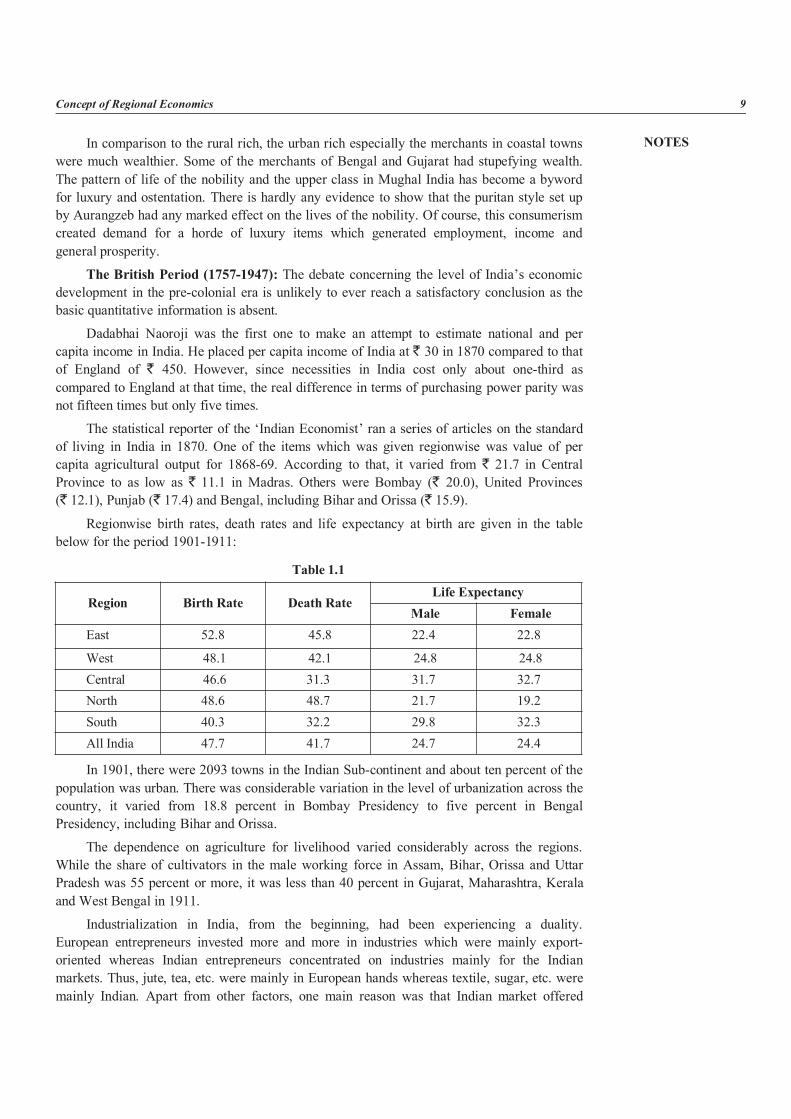
Regionwise birth rates, death rates and life expectancy at birth are given in the tablebelow for the period 1901-1911:

Table 1.1

Region Birth Rate Death RateLife Expectancy

Male FemaleEast 52.8 45.8 22.4 22.8

West 48.1 42.1 24.8 24.8Central 46.6 31.3 31.7 32.7North 48.6 48.7 21.7 19.2South 40.3 32.2 29.8 32.3All India 47.7 41.7 24.7 24.4

In 1901, there were 2093 towns in the Indian Sub-continent and about ten percent of thepopulation was urban. There was considerable variation in the level of urbanization across thecountry, it varied from 18.8 percent in Bombay Presidency to five percent in BengalPresidency, including Bihar and Orissa.

The dependence on agriculture for livelihood varied considerably across the regions.While the share of cultivators in the male working force in Assam, Bihar, Orissa and UttarPradesh was 55 percent or more, it was less than 40 percent in Gujarat, Maharashtra, Keralaand West Bengal in 1911.

Industrialization in India, from the beginning, had been experiencing a duality.European entrepreneurs invested more and more in industries which were mainly export-oriented whereas Indian entrepreneurs concentrated on industries mainly for the Indianmarkets. Thus, jute, tea, etc. were mainly in European hands whereas textile, sugar, etc. weremainly Indian. Apart from other factors, one main reason was that Indian market offered

NOTES


higher profit margins which Indian industrialists found easier to penetrate. Not surprisingly,this tendency continues even today.

The benefit of irrigation development was mainly concentrated in northern, western andsouthern provinces during British period. Central and Eastern India were relatively neglected.This has had serious implications in the post-independence period also. While the formerareas were ripe for benefiting from the green revolution package, the latter could not.

From its beginning in 1853, India’s railway system expanded rapidly to become, by1910, the fourth-largest in the world. This network which covered most of the Sub-continent,radically altered India’s transportation system.

Railways vastly increased the speed, availability and reliability of transportation,reduced the cost, allowed regional specialization and expansion of trade. For attractingprivate investors, Government of British India assured guaranteed return. Under this scheme,which was used in other parts of the world to build railways, if a company did not attain aminimum rate of return of five percent, it received compensation for the difference from theGovernment. Stimulated by an assured rate of return, British investors swiftly made theircapital available to the private railway companies. By 1947, all but a few remote districts infar-flung remote regions were served by railways.

The fiscal system during the British rule gradually evolved into a federal system from ahighly centralized control. Over the years, relations between the centre and the provinceswere made more elastic but not much more systematic. In particular, there was no attempt toequalize provincial levels of public services, or the tax burdens on similar classes of taxpayers in different States. There were enormous differences in tax incidence and standards ofpublic services in the beginning, and these differences were perpetuated since precedent wasfollowed rather than any principle.

The main source of differences in tax burdens was the variation in the system of landrevenue, the largest source of public revenue. This also explained one source of difference inexpenditure. Bombay spent much more per head on nearly every head of expenditure than theothers. The other provinces clamoured for less inequality but to little effect. Bombaycontinued to spend far more on every major head than the other provinces, and Bihar andOrissa far less. The poverty of these provinces became evident when they were separatedfrom Bengal in 1912-13.

Many critics also argued that the system did not even encourage economy, but ratherextravagance, since the actual expenditure in one period formed the basis of allocations fromthe centre in the next. For the same reason, the provinces had little incentive to try to raisetheir tax revenues. A more or less similar situation exists in India even today when theFinance Commissions assess the revenue gaps of the States and try to fill such gaps byincreased transfers.

Post-Independence Period: Government’s economic policies during the colonialperiod were more to protect the interests of the British economy rather than for advancing thewelfare of the Indians. The primary concerns of the Government were law and order, taxcollection and defence. As for development, Government adopted a basically laissez-faireattitude. Of course, railways, irrigation systems, road network and modern education systemwere developed during this period. Railways and road network were more to facilitatemovements of goods and defence personnel and to facilitate better administrative control.Irrigation canal system was mainly to fight repeated droughts and famines and to boost land

NOTES


revenue. Education, to begin with, was developed mainly to train lower-ranking functionariesfor the colonial administration.

Particularly lacking was a sustained positive policy to promote indigenous industry.Indeed, it is widely believed that government policies, far from encouraging development,were responsible for the decline and disappearance of much of India’s traditional industry.

Altogether, the pre-independence period was a period of near stagnation for the Indianeconomy. The growth of aggregate real output during the first half of the twentieth century isestimated at less than two percent per year, and per capita output by half of a percent a yearor less.

There was hardly any change in the structure of production or in productivity levels. Thegrowth of modern manufacturing was probably neutralized by the displacement of traditionalcrafts, and in any case, was too small to make a difference to the overall picture.

Along with an impoverished economy, independent India also inherited some usefulassets in the form of a national transport system, an administrative apparatus in working order,a shelf of concrete development projects and a comfortable level of foreign exchange. Whileit is arguable whether the administrative apparatus built by the British helped or hindereddevelopment since 1947, there is little doubt that its existence was a great help in coping withthe massive problems in the wake of independence such as restoring civil order, organizingrelief and rehabilitation for millions of refugees and integrating the Princely States to theUnion.

The development projects initiated in 1944 as a part of the Post-war ReconstructionProgramme was of particular value to Independent India’s first government. Under theguidance of the Planning and Development Department created by the Central Government, agreat deal of useful work was done before Independence to outline the broad strategy andpolicies for developing major sectors and to translate them into programmes and projects. Bythe time of Independence, several of these were already under way or ready to be taken up.They included programmes and projects in agriculture, irrigation, fertilizer, railways,newsprint and so on. Though the first Five Year Plan began in 1950-51, with theestablishment of Planning Commission, a well-rounded planning framework was in placeonly with the second Five Year Plan after five years. By and large, the basis of the first FiveYear Plan was the groundwork done before independence. Most of the principal projectswere continuations and major efforts were made to complete them early.

II. Recent TrendsIndian economy has experienced an average annual growth rate of around 6 percent

during the last two decades. Though, moderate compared to the performance of several EastAsian economies during the same period, this was quite impressive compared to theperformance of Indian economy during the preceding three decades when the average growthlogged 3.5 percent per annum. Even the growth rate of 3.5 percent experienced during thefirst three decades of the republic had been spectacularly better that the virtual stagnation ofthe Indian economy during the first half of the Twentieth century. In terms of per capitaincome, the improvement has been even more remarkable — around 4 percent per annum inthe recent period as compared to less than 1.5 percent in the earlier period. Further, during therecent period, there has been a steady acceleration in the growth performance over the years.The average compound growth per annum was 5.7 percent during the Sixth Five Year Plan(1980-85), 6.0 percent during the Seventh Plan (1985-90), 6.6 percent during the Eighth Plan(1992-97) and subsequently 8 percent during Twelfth Plan (2012-17). While the growth rate

NOTES


dropped to 3.1 percent during the two-year period 1990-92 in the wake of internationalpayment crisis and the introduction of major economic reforms, the growth process picked upfast in the subsequent years. Indeed, the growth averaged about 7.5 percent during the three-year period ending 1996-97, which is impressive by any standards. The growth rate has beensomewhat lower in the subsequent three years. In contrast to stagnation or negative growth ofmost of the East Asian economies, India’s performance, however, is remarkable. The WorldBank and other international agencies have characterized India as one of the fastest growingeconomies of the world. With the economy slowing down and figures for the year notoptimistic, the Planning Commission plans to seek a lowering of the growth rate for the12th Five Year Plan to 8 percent at the meeting of the National Development Council (NDC)in Delhi. Core objective is that we should be going in for a more optimistic scenario andprobably if we reflect, what we now know is that instead of 8.2 percent, it would be better topitch it at 8 percent.

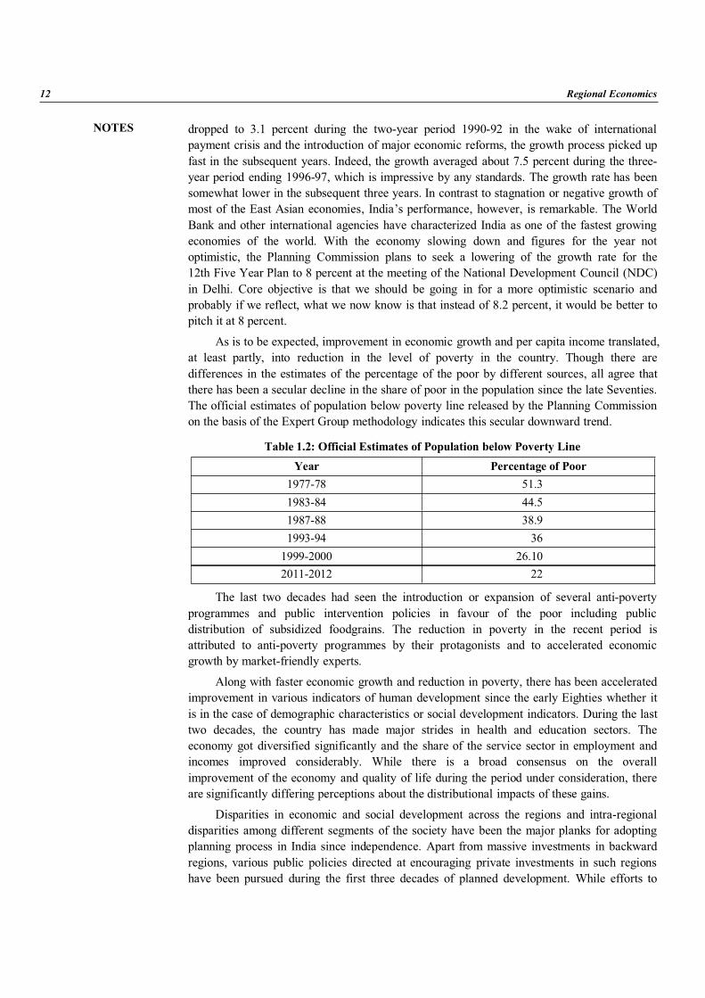
As is to be expected, improvement in economic growth and per capita income translated,at least partly, into reduction in the level of poverty in the country. Though there aredifferences in the estimates of the percentage of the poor by different sources, all agree thatthere has been a secular decline in the share of poor in the population since the late Seventies.The official estimates of population below poverty line released by the Planning Commissionon the basis of the Expert Group methodology indicates this secular downward trend.

Table 1.2: Official Estimates of Population below Poverty LineYear Percentage of Poor

1977-78 51.31983-84 44.51987-88 38.91993-94 36

1999-2000 26.102011-2012 22

The last two decades had seen the introduction or expansion of several anti-povertyprogrammes and public intervention policies in favour of the poor including publicdistribution of subsidized foodgrains. The reduction in poverty in the recent period isattributed to anti-poverty programmes by their protagonists and to accelerated economicgrowth by market-friendly experts.

Along with faster economic growth and reduction in poverty, there has been acceleratedimprovement in various indicators of human development since the early Eighties whether itis in the case of demographic characteristics or social development indicators. During the lasttwo decades, the country has made major strides in health and education sectors. Theeconomy got diversified significantly and the share of the service sector in employment andincomes improved considerably. While there is a broad consensus on the overallimprovement of the economy and quality of life during the period under consideration, thereare significantly differing perceptions about the distributional impacts of these gains.

Disparities in economic and social development across the regions and intra-regionaldisparities among different segments of the society have been the major planks for adoptingplanning process in India since independence. Apart from massive investments in backwardregions, various public policies directed at encouraging private investments in such regionshave been pursued during the first three decades of planned development. While efforts to

NOTES


reduce regional disparities were not lacking, achievements were not often commensurate withthese efforts. Considerable level of regional disparities remained at the end of the Seventies.The accelerated economic growth since the early Eighties appears to have aggravatedregional disparities. The ongoing economic reforms since 1991 with stabilization andderegulation policies as their central pieces seem to have further widened the regionaldisparities. The seriousness of the emerging acute regional imbalances has not yet receivedthe public attention it deserves.

Most of the studies on inter-country and inter-regional differences in levels of living andincome are done within the theoretical framework of neoclassical growth models. Thesemodels, under plausible assumptions, demonstrate convergence of incomes. Three notablerecent studies, however, indicate that in the Indian context these convergence theories do notexplain the ground realities.

The scope of analysis in this section is restricted to a comparative analysis of theemerging trends in fifteen major States in respect of a few key parameters which have anintrinsic bearing on social and economic development. The variables chosen for examinationinclude those which have a bearing on gender and equity issues. The fifteen States togetheraccount for 95.5 percent of the population of India. The remaining 4.5 percent of thepopulation is spread out in 10 smaller States and seven Union Territories including theNational Capital Territory of Delhi. Leaving out these States and UTs from detailed study ismainly due to non-availability of all relevant data and also to keep the data sets analyticallyand logistically manageable. The fifteen States taken up for the detailed study have beengrouped into two – a forward group and a backward group. The forward group consists ofAndhra Pradesh, Gujarat, Haryana, Karnataka, Kerala, Maharashtra, Punjab and Tamil Nadu.The backward group comprises of Assam, Bihar, Madhya Pradesh, Orissa, Rajasthan, UttarPradesh and West Bengal.

Geographically, the forward group of States fall in the Western and Southern parts ofthe country and are contiguous except for Punjab and Haryana which are separated byRajasthan from the rest of the States in this group. The group of backward States are in theEastern and Northern parts of the country and are geographically contiguous. Another notablegeographical feature is that while six out of eight States, except Haryana and Punjab, in thefirst group have vast sea coasts, only two out of the seven in the second group, viz., Orissaand West Bengal are littoral. While the forward group of States account for about 40.4 percentof the national population, the backward group accounts for as much as 55.1 percent of thepopulation of the country according to 2001 census. In terms of natural resources includingmineral wealth, water resources and quality of soil, the latter has definite edge over theformer.

A limitation of inter-regional analysis using States as units is the fact that this may notbe able to capture the significant intra-State disparities in economic and social development,which exists today. The larger States in both the groups have regions within themselves,which are vastly different in terms of various indicators of development. There areidentifiable distinct regions, at different stages of development, in several States.

Demographic and Social Characteristics: As noted earlier, the group of eight forwardStates together accounted for 40.4 percent of the population of the country whereas the groupof seven backward States together accounted for as much as 55.17 percent of the populationof the country according to 2001 census. However, the contribution of the group of forwardStates to the country’s population growth during the last decade was much higher at59.2 percent. On the other hand, the contribution of the group of backward States was as low

NOTES


as 33.8 percent. All the States, except Assam and Orissa, in the backward group had a highercontribution to population growth than their share in population. Thus, Uttar Pradesh’scontribution to population growth was 18.8 percent against its population share of16.2 percent and Bihar’s contribution was 10.1 against its share of population of 8.17 percent.

In contrast, out of the eight States in the forward group, all except Maharashtra, Gujaratand Haryana had a lower contribution to population growth during the last decade than theirrespective shares in the population. Indeed, Kerala’s contribution to population growth was aslow as 1.5 percent against its share in the population of 3.1 percent and Tamil Nadu’scontribution to population growth was as low as 3.4 percent against its share in the populationof 6.1 percent.

To broadly characterize, the two groups of States are at different stages of demographictransition. States like Kerala and Tamil Nadu which have already reduced their birth rates tolevels are comparable to those of developed countries and achieved the replacement level oftotal fertility rate (TFR) of 2.1. All the remaining six States of the forward group are expectedto reach the replacement level of TFR by 2025, one year in advance of the projected year ofattainment of replacement level of TFR by the country. On the other hand, the seven States inthe backward group are at different stages of demographic transition. Some of them like UttarPradesh, Bihar, Madhya Pradesh and Rajasthan continue to experience high rate of birth ratesand fairly low levels of death rates and a significantly high level of TFR. On the other hand,States like Assam, Orissa and West Bengal have somewhat moderate birth and death ratesand relatively moderate TFR. These three States are expected to reduce their TFR toreplacement level well before the country’s TFR comes down to that level. As against this,Bihar is expedited to reduce TFR to replacement level by 2039, Rajasthan by 2048, MadhyaPradesh by 2060 and Uttar Pradesh beyond 2100.

According to 2001 census, the literacy rate for the country is 65.4 percent. All States inthe forward group, except Andhra Pradesh, have literacy rates above the national average. Theirrates vary from 90.9 percent in Kerala to 67.0 percent in Karnataka. The level of literacy inAndhra Pradesh is only 61.1 percent. In the backward group, all except West Bengal haveliteracy rates below national average. They vary from 64.3 percent in Assam to as low as 47.5percent in Bihar. The level of literacy in West Bengal is 69.2 percent.

Census 2001 indicates that the gender gap in literacy has come down for the countryfrom 24.8 percentage points in 1991 to 21.7 percentage points in 2001. Now, the maleliteracy is 76.0 percent and female literacy is 54.3. On the whole, the literacy gap is lower inthe forward group of States as compared to the backward group of States. Six out of eightStates in the first group, except Haryana and Gujarat, have literacy gaps below the nationalaverage. On the other hand, all States except Assam and West Bengal have gender gap inliteracy higher than the national average. The gender gap in literacy is as low as 6.3percentage points in Kerala and as high as 32.1 percentage points in Rajasthan. There appearsto exist a strong inverse relationship between the gender gap in literacy and the status ofwomen in society. Also, there is a fairly well-established inverse empirical relationshipbetween the female literacy and TFR. The national as well as international experience is thatwith higher female literacy rate, birth rate come down irrespective of the social backgrounds,religious beliefs and income levels.

The group of backward States account for 63.3 percent of the illiterate females in thecountry, a share which far exceeds its population share. On the other hand, the group offorward States account for only 34.4 percent of the illiterate in the country, a share far less

NOTES


than its population share. In this group, Andhra Pradesh is the only State where the share ofilliterate females is higher than the share of population.

Income and Property: The most common indicator of the economic development of asociety is the per capita annual income generated by it. The level of poverty or the share ofpopulation which do not have minimum income to meet its basic requirements is an indicatorof the level of economic development as well as the inequality in the income distribution.

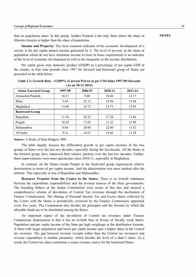
Per capita gross state domestic product (GSDP) as a percentage of per capita GDP ofthe country at four time periods since 1997 for forward and backward group of States arepresented in the table below:

Table 1.3: Growth Rate – GSDP% (Current Prices) as per CSO Data 1997-98 Onwards(As on 30-11-2014)

States Forward Group 1997-98 2006-07 2010-11 2013-14Arunachal Pradesh 10.31 9.40 20.66 14.17Bihar 3.44 22.12 24.94 15.84Meghalaya 13.60 18.72 14.75 15.03Backward GroupRajasthan 11.38 20.25 27.28 11.86Punjab 10.20 17.02 21.22 12.90Maharashtra 8.84 20.08 22.60 11.52All India N.A 16.67 18.66 11.54

Source:A Study of State Budgets: RBI.

The table sharply focuses the differential growth in per capita incomes of the twogroups of States over the last two decades, especially during the last decade. All the States inthe forward group, have improved their relative position over the last two decades. Further,these improvements were more spectacular since 2010-11, especially in Meghalaya.

In contrast, all the States except Punjab in the backward group experienced relativedeterioration in terms of per capita income. And the deterioration was more marked after thereforms. This especially is true of Rajasthan and Maharashtra.

Resource Transfer from the Centre to the States: There is an in-built imbalancebetween the expenditure responsibilities and the revenue sources of the State governments.The founding fathers of the Indian Constitution were aware of this fact and ensured acomprehensive scheme of devolution of Central Tax revenues through the mechanism ofFinance Commissions. The sharing of Personal Income Tax and Excise duties collected bythe Centre with the States is periodically reviewed by the Finance Commission appointedevery five years. The Commission also decides the principles and the formula by which theallocable funds are to be distributed among the States.

An important aspect of the devolution of Central tax revenues under FinanceCommission dispensation is that it has an in-built bias in favour of fiscally weak States.Population and per capita income of the State get high weightage in the distribution formula.A State with larger population and lower per capita income gets a higher share in the Centraltax revenues. The gap between revenue receipts (other than the Central tax revenues) andrevenue expenditure is another parameter, which decides the level of a State’s share. As aresult, the Central tax share constitutes a major revenue source for the backward States.

NOTES


A second channel of resources flow from the Centre to the States is PlanningCommission, which provides Central Assistance for State Plans. The State plans are financedpartly by States’ own resources and the balance by Central Assistance. Central assistance isprovided as a block assistance of which 30 percent is grant and the remaining 70 percent is along-term loan. The rationale for this grant-loan proportion is imbedded in the fact that about30 percent of the plan expenditure was of revenue nature and 70 percent was of capital naturewhen this proportion was decided in the late Sixties. Since plan expenditure of revenue natureis not expected to yield any financial returns for servicing the loan, this share was provided asgrant by the Centre.

The distribution of Plan assistance to the States has been governed by ‘Gadgil Formula’since the Fourth Five Year Plan (1969-74). As in the case of Finance Commission devolution,‘Gadgil Formula’ which is administered by the Planning Commission also has its built-in biasin favour of backward States. Population and per capita income together account for85 percent of the weight in the formula. The remaining 15 percent weightage is equallydivided between State performance in the achievement of certain priority national objectivesand the special problems of the States. Central assistance constituted about 45 percent of theState Plans when all States are taken together. While the share of Central assistanceconstitutes less than 25 percent of the Plan finances of the more developed States, itaccounted for the major share of Plan finances of the backward States. Indeed, the Plans ofthe most backward States, especially the Special Category States, have been fully financed byCentral Assistance.

In the wake of the foreign exchange crisis in the early nineties, the Centre has beenencouraging States to seek and absorb more and more external aid for development projects.The external aid to the States is routed through Central budget and devolved as additionalCentral Assistance for State plan on the same terms and conditions as the normal Centralassistance to the State Plans. From the early Nineties, there has been a substantial increase inaid flows to the States. However, the major share of such flows have been absorbed by a fewdeveloped States. As a result, during the nineties, there has been an apparent increase in theCentral assistance to the more developed States. While ‘Gadgil Formula’ based normalCentral assistance continued to be positively discriminating towards backward States,additional Central assistance for externally aided projects was skewed towards better offStates. Indeed, external aid accounted for 40 to 60 percent of Central Plan assistance to someof the developed States, while such assistance contributed less than 10 percent of the CentralPlan assistance to most of the backward States.

However, although it is true that resource flows through the Finance Commission andPlanning Commission account for a substantial share of State resources, whose overallimpacts are highly beneficial to the fiscal health of the tates, yet there are certain adverseeffects of such flows on the State finances. First, since the Finance Commission approach torevenue deficit is basically a gap-filling approach, this diminishes the incentive of the Statesto raise revenue receipts and reduce revenue expenditure. In other words, there is an implicitpremium on fiscal profligacy. Second, continuing expenditure on plan schemes beyond theFive Year Plans became the committed expenditure of the States and add to their fiscalburden. Since there is a premium on plan expenditure, State governments have a tendency tounder-fund maintenance expenditure to inflate the plan size. This results in poor maintenanceof public assets created in the past and poor quality of public services, which are outside theplan. A further complication is due to steep increase in the revenue component of planexpenditure over the years. While the grant-loan ratio of Central assistance is still 30 : 70, the

NOTES


revenue share of State Plan expenditure has reached almost 60 percent. As a result, the debt-servicing burden of the States has gone up significantly.

Pattern of Private Investment: In the wake of economic reforms initiated in 1991, therole of private investment has acquired a special significance in the context of economicdevelopment of various States of the Indian Union. Indeed, there has been an element ofcompetition among States ever since for attracting private investment, both domestic andforeign. Some of the States have been offering various tax concessions and other specialfacilities to new investors on a competitive basis.

The total investment proposals received by all the States and UTs since the inception ofeconomic reforms in August 1991 till the end of March, 2000 are worth ` 9,08,888 crore.Disparities are obvious. States like Andhra Pradesh, Gujarat and Haryana accounted for two-third of the amount while states such as Assam, Madhya Pradesh, Uttar Pradesh accountedfor just over 27 percent of the amount. Indeed, Gujarat and Maharashtra together accountedfor 39 percent of the investment proposals, which is significantly more than the totalinvestment proposals received by States such as Assam, Madhya Pradesh and Uttar Pradesh.While Gujarat which accounted for less than 5 percent of the population of the country,received over 17 percent of the private investment proposals, Bihar which accounts for morethan 10 percent of the population of the country, received just a little over one percent of suchproposals. This is a clear pointer to the direction of private investment in the coming years.

As regards shares of different States in bank deposits, it is found inter-State and regionaldisparities. While states like Andhra Pradesh, Gujarat, Haryana, Karnataka, Kerala etc.account for over 54 percent of the bank deposits, on contrary States like Assam, Rajasthanand Uttar Pradesh accounts for only about 31 percent of the bank deposits. Maharashtra aloneaccounts for about 20 percent of the bank deposits.

The distribution of bank credit across the States given shows that bank creditdistribution is even more skewed than bank deposit distribution. It implies that a part of thedeposits mobilized in the backward States is getting transferred to the advanced States. Whilethe first group of States accounted for about 65 percent of the bank credit, the second groupof States could receive only about 21 percent of the bank credit. Indeed, Maharashtra aloneaccounted for more bank credit than all the seven States in the second group put together.Similarly, all the States in the second group, except Uttar Pradesh and West Bengal, puttogether received less bank credit than Tamil Nadu. The implications of such skeweddistribution of bank credit across the States on economic growth and income distribution inthe coming years are obvious. The fact that Maharashtra and Tamil Nadu have major metrosin them might have helped them to get higher share of bank credit. Having Calcutta as theState capital might have helped West Bengal also somewhat. In this context, it may be ofinterest to note that all the 15 States considered together which account for 96.5 percent of thepopulation of the country accounted for only around 85 percent of bank deposit and bankcredit. The fact that the remaining 15 percent have gone to the minor States and UTs may besomewhat surprising. This, however, is because of NCT of Delhi accounting for over10 percent of bank deposits and bank credit.

Apart from that, so far as credit-deposit ratios for different States are concerned, itcaptures the discrepancy in credit absorption vis-a-vis deposit mobilization. Exceptions apart,credit-deposit ratios are much more favourable to the States like Andhra Pradesh, Gujarat,Haryana etc.as compared to States like Assam, Rajasthan, Uttar Pradesh etc..

NOTES


III. Intra-state DisparitiesIn the foregoing sections, we have studied various dimensions of inter-State disparities.

An important aspect of regional disparities in India, which could not be covered by thisapproach, is the significant level of regional disparities, which exist within different States.An important cause of regional tensions which lead to popular agitation and at times militantactivities is such regional disparities in economic and social development which exist withinsome of the States. Indeed, creation of some of the States in the past was in the wake ofpopular agitation based on perceived neglect of certain backward regions in some of thebigger States. The best instances of such cases are the creation of Andhra Pradesh andGujarat in the Fifties and creation of Punjab, Haryana and Himachal Pradesh in the Sixties.The latest example is the creation of three new States caved out from an existing larger State,viz., Madhya Pradesh, Bihar and Uttar Pradesh respectively. Past experience, by and large, isthat when two or more States are carved out from an existing one or a new State is created bycombining parts from more than one State on the basis of some homogeneity criterion likelanguage or some other common heritage, the newly created States develop faster than thepre-partition States.

A number of States included in our analysis have clearly identifiable regions which areat different stages of development and which have distinct problems to tackle. Creation ofnew States, certainly, may not be a solution to such regional disparities. At the same time, itis important to recognize such intra-state regional disparities explicitly and tackle themthrough special efforts. As we have noted in an earlier section, Maharashtra is a typicalexample of a State where overall development is quite good in terms of almost all indicators,but extreme regional disparities exist. Andhra Pradesh has three distinct regions which are atdifferent stages of socio-economic development, viz., Coastal Andhra, Telangana andRayalaseema. Similarly, North Bihar and South Bihar before State reorganization in 2000were at different stages of development with entirely different problems. Uttar Pradesh, evenafter caving out Uttaranchal, has at least three regions with varying problems and differentlevels of socio-economic development. Other States like Gujarat, Karnataka, Madhya Pradesh,Orissa, Rajasthan and West Bengal also have regions with distinct characteristics ofbackwardness.

A closer examination of the nature of backward regions in each State will indicatespecific reasons for their backwardness. The major cause of backwardness of Vidharba andMarathwada in Maharashtra, Rayalaseema and Telangana in Andhra Pradesh and NorthernKarnataka is the scarcity of water due to lower precipitation and lack of other perennialsources of water. On the other hand, backwardness of certain regions in Gujarat, MadhyaPradesh, Bihar and Orissa can be associated with the distinct style of living of the inhabitantsof such regions who are mostly tribals and the neglect of such regions by the ruling elite.Topography of a region could also constrain the development of that region; the desert regionof Rajasthan is an example of such a case. Historical factors like the attitude of rulers of theformer Princely States towards development could have significantly affected thedevelopment of a region. For example, the distinctly higher level of social development of theTravancore and Cochin regions of Kerala can be traced back to the enlightened attitude of theformer rulers of the Princely States of Travancore and Cochin. On the other hand, the poorsocial development of Telangana region of AP and certain other parts of the Deccan could betraced back to the absence of visionary rulers in the respective princely States.

An important question, however, is why after 50 years of planned development efforts,such intra-State disparities remain unattended? Often, the answer depends on whether it is

NOTES


given by people who are the victims of underdevelopment or not. The representatives of thebackward regions often attribute the cause of their backwardness as neglect on the part of therulers of the State, who are often from the well heeled regions. The ruling class may come upwith any number of explanations for the underdevelopment of backward regions, which arebeyond their control. Indeed, there are specific institutional arrangements for development ofbackward regions in some of the States. Maharashtra and Uttar Pradesh (before Statereorganization) are two such instances. In Maharashtra, there are separate regional plans forthe backward regions. In Uttar Pradesh, there was a separate regional plan for the hill regionwhich is characterised as Uttarakhand.

Besides the State-specific efforts for reducing intra-State regional disparities, a numberof Centrally Sponsored Programmes have been in operation for the last two to three decadesfor taking care of specific aspects of backwardness of such regions. The Tribal DevelopmentProgramme, the Hill Area Development Programme, the Western Ghat DevelopmentProgramme, the Drought Prone Area Programme and Desert Development Programme areexamples of such ongoing efforts. The evaluation studies of some of these programmes haveindicated clearly identifiable benefits of such programmes, though at the same time criticizedthese programmes for their cost-ineffectiveness due to various drawbacks in their design,planning and implementation. Often they are conceived, planned and implemented by thebureaucracy without any involvement of the local people. More often, discontent andagitation on the basis of perceived neglect of the backward regions by the rulers at the Statelevel and at the Centre are led by local leaders who demand some form of autonomy todetermine their own destiny. Even those who demand separate State for their region are oftenwilling to settle for autonomous regions within the existing State with considerable financialand administrative powers. The problem, however, is that the State level rulers are generallyunwilling to part with their own power of patronage. Those who demand more autonomy forthe States from the Centre are often unwilling to share power, either administrative orfinancial, with the elected local bodies. Indeed, with the 73rd Amendment Act of theConstitution, the Panchayat Raj Institutions were expected to function as local governmentswith sufficient finances and functions to take care of most of the developmental functions. Ifthey are allowed to function as responsible self-governing local governments, considerableground can be covered to reduce the regional disparities within the States.

Before concluding this Section, we may mention a few successful cases, where intra-State regional disparities have been reduced considerably through public policies. First, in1956 when Kerala was formed at the time of State reorganization, there was substantialdisparity in the social development of Malabar region vis-a-vis the Travancore-Cochin region.Over the last four decades, there has been remarkable improvement in the social indicators ofMalabar to catch up with the rest of Kerala as a result of appropriate public policies. Thedevelopment of the drought prone districts of Haryana through irrigation is anotherremarkable example of reduction in economic disparities across the regions within a State.Provision of educational, health and communication facilities even in the remotest villages ofHimachal Pradesh is a third example of successful public policies in reduction of regionaldisparities within a State. Overall, Tamil Nadu could be considered as one State which ismost successful in reducing regional disparities in economic and social development evenwhen there was substantial variation in the natural endowments in different parts of the State.This was achieved by a combination of public policies and private initiatives. In other States,especially in Maharashtra, Gujarat and Rajasthan, there are a number of successful cases ofNGOs which succeeded in transforming pockets of destitution into areas enjoying very highlevels of socio-economic development.

NOTES


IV. Profile of Regional Disparities for Different Growth Scenarios 2025An analysis of the historical trends, especially the more recent trends, leads to the

inevitable inference that regional disparities are bound to aggregate in the coming decades.Regions, which are characterized as backward in our foregoing discussions, have very weakgrowth impulses.

Their demographic disadvantage is implicit in the fact that major States in this region,viz., Bihar, Madhya Pradesh, Rajasthan and Uttar Pradesh are likely to have fertility ratesexceeding the replacement level well beyond 2025, a level which some of the forward Stateslike Kerala and Tamil Nadu have already achieved and others are expected to achieve withina decade or so. We have noted that if the current trend is projected, Madhya Pradesh willreach replacement level only by 2060, and Uttar Pradesh only by 2100.

The implications of these divergent demographic trends on population density,employment opportunities, social sector investments and the overall development can beextremely grave. One of the major objectives of development planning initiated immediatelyafter Independence has been, among others, reduction of regional disparities in social andeconomic development. Direct investment by the Central Government and Centrally directedinvestment of the private sector have been two powerful instruments to achieve this objective.

During the first four decades of development planning, most of the large units in basicand heavy industries were set up in the public sector in a regionally well-balanced manner.Indeed, their location, other things being equal, was biased towards backward regions asnatural endowments such as mineral deposits were concentrated in those regions. Massivepublic investments have been made to provide economic and social infrastructure in thebackward regions to accelerate their overall development.

The natural tendency of the private sector is to set up industries and other relatedactivities in developed regions. To counter-balance this tendency, various incentive anddisincentive schemes have been introduced as public policies to direct private investments tobackward regions. Fright equalization scheme was just one of them. The efforts of the firstfour decades of planned development to reduce various imbalances across the regions havebeen only partially successful. At best, they have ensured that regional disparities in terms ofvarious indicators of development are not aggravating. Of course, even this is no meanachievement.

Economic reforms initiated in 1991 implied among, other things, that the private sectorwould be the principal engine of economic growth. Most of the restrictions on privateinvestment have been removed. Mounting debt burden of the government has imposed a capon public investment. As a result, while there was significant increase in the quantum ofprivate investment, there was a sharp fall in the public investment over the last decade.

The flow of private investment, both domestic and foreign, has been extremely biased infavour of the more developed regions of the country. This has enabled the developed regionsto achieve accelerated economic growth during the 1990s. On the other hand, backwardregions of the country, which were unable to attract any significant private investment flows,experienced decelerated economic growth during this period.

The net result of this divergent growth performance of the developed and backwardregions has been a widening of the regional disparities in the country in terms of per capitaincome and other indicators of well-being of the people.

The ability of the governments at the Centre and in the States to counter this trend byeffecting countervailing public investment also has been reduced considerably. In the context

NOTES


of macroeconomic stabilization policies initiated in 1991, the ability of the Centre to financepublic investment by borrowings has been severely constrained. Revenues of the Centre alsoexperienced reduced buoyancy in the wake of tax reforms especially due to reduction incustoms tariff to levels comparable to those of our trading partners.

The factors which attracted more and more private investments to developed regionshave been their better developed economic and social infrastructure as well as more efficientand investor friendly State governments. The backward regions, to be attractive to the privateinvestors, have to improve their infrastructure facilities, both economic and social,considerably. This needs substantial public investment. The State governments in thebackward regions are, however, strapped for funds even to meet the current expenditure.

Almost all the State governments in the backward regions find that their entire revenuesare not sufficient to meet even the committed revenue expenditure like interest liability,salaries and pensions. A sizable share of their borrowings is diverted to fill the gap betweenthe revenue receipts and revenue expenditure. There are several States where borrowingshave been steadily increasing, but investments have been decreasing secularly.

The adverse impacts of the deteriorating State finances are much more severe for thebackward States as compared to the developed States, where investments of the past havecreated adequate social and economic infrastructure to attract private investments. Thebackward States are facing multiple dilemma. They are not able to attract investments due tolack of infrastructure. They are not in a position to provide these facilities on their own due tolack of investible funds. Unlike in the past, Centre is not in a position to help them either asthe Centre itself has a serious fiscal constraint.

Along with social and economic infrastructure, efficiency of administration and thequality of governance including law and order situation are important factors in attractingprivate investment. Studies conducted by NCAER and some of the apex associations ofindustries have indicated that prospective investors give higher weightage to these factorsthan various incentives, including fiscal incentives offered by the State governments. Indeed,there are enough evidences to the effect that the investors don’t mind paying speed money toget things done fast. In other words, a corrupt but efficient regime is preferred to an honestbut inefficient regime in the context of investment decisions. Other aspects of governancelike the law and order situation, trade union activism, etc. are also important factors affectingthe flow of private investments.

On almost all indicators of governance discussed above, the backward States are at adisadvantage. Indeed, even perceptions about the governance issues based on past may hauntthe States in such matters. The cases of Kerala and West Bengal are typical in this regard. Allthe efforts of these two States during the last decade to woo the investors, both domestic andforeign, have not yielded any significant results. This was mainly on account of the generalperception of investors that these States are dens of militant trade union activism, though inreality such militancy, of late, has been significantly subdued in these States.

To conclude this section, it will be appropriate to state that there are hardly any signs ofreversing the recent trend of accentuating regional disparities in the country in the comingdecades. Indeed, almost all the relevant forces are such that the disparities are likely to widenderiving the next quarter century. It will require Herculean tasks on the part of the Centre andthe leadership in the concerned regions to ensure that the gap does not widen further.

NOTES


V. Impact on Political, Social and Economic StabilityIt comes out clearly from the discussions in the preceding section that if the past trends,

especially those of the recent past continued for the next two decades or so, India will be ahighly uneven nation in terms of various dimensions of public life. Incomes and livingstandards will vary considerably across the nation. People in most of the southern andwestern parts of the country will be enjoying fairly high per capita incomes, which may becomparable to those of middle income developed countries today. More than half of thepeople in this part of the country will be living in cities and towns with all modern facilities.Even in rural areas, amenities of modern life and reasonably efficient civic facilities will beavailable. Almost all the children of school-going ages will be attending schooling. There willbe hardly any difference between boys and girls in school. The gender difference in literacywill have almost disappeared. Population growth might have come down below replacementlevel in all the States in this region. A few States like Kerala and Tamil Nadu might havereached stable population level. The average health and nutrition level might have increasedsignificantly. Life expectancy in all States of this region might have crossed 70, both for menand women.

The sectoral employment and incomes will have changed considerably. The share ofagriculture in the State domestic product will be 10 to 20 percent in different States and thepopulation dependent on agriculture will be 20 to 40 percent. The share of tertiary sector inemployment and income will have increased significantly and accounting for 30 to 40 percentof employment and 50 to 60 percent of income. Secondary sector will account for the balance.

On the whole, productivity of labour will be increased substantially in all the sectorsmainly on account of new technologies and skill-endowed labour forces. As a result ofsecular economic growth of 8 to 10 percent for over two decades and negligible populationgrowth, per capita incomes in the region will have nearly quadrupled as compared to today.Even in agriculture, which would have been highly diversified and market-oriented, incomeswill have gone up significantly. Also, because of effective watershed management, even inthe drought prone areas, yearly fluctuations of agricultural output will have been minimal.

Abject poverty and deprivations will be unheard of. An effective food security andsocial security administered by the Village Panchayats takes care of the needs of the poor.The Panchayats will administer most of the civic facilities as well as social and economicinfrastructure and services. A similar situation will prevail in the urban areas also. One of themajor problems in the larger cities, however, will be ensuring civic facilities and housing forthe migrant labour from the other parts of the country.

VI. Policy Initiatives for Balanced Regional GrowthWe shall initiate the discussion on initiatives for balanced regional growth by

illustrating two instances of initiatives in the past. One relates to agriculture and the otherrelates to industry, the two most important sectors of our economy. The strategy to boostagricultural production and to ensure food security was evolved in the mid-Sixties when thecountry faced a grim situation following two consequent years of severe drought. Thestrategy consisted of various incentives to farmers to adopt high yielding seeds of wheat andpaddy along with complimentary inputs, assured minimum support prices for the output,buffer stocking of the foodgrains and supplying the same to the States to distribute throughthe public distribution system (PDS) to the consumers, especially in the deficit regions. Toback up this strategy, institutions like Agricultural Prices Commission (APC), FoodCorporation of India (FCI) and Warehousing Corporation of India and other ancillary

NOTES


institutions were established. Arrangements were made to spread the message of highyielding seeds and the associated package of inputs and practices.

The above strategy ushered in a green revolution, which resulted in doubling of wheatand rice production in the country over a short period. Adequate foodgrains surpluses weregenerated to build up the needed buffer stock. India was no more a basket case.

The initial success of green revolution strategy was restricted to Punjab, Haryana andwestern Uttar Pradesh where assured irrigation networks already existed. Subsequently, itwas extended to a few irrigation commands in the South and West also. It was, however,expected that with the expansion of assured irrigation, the green revolution would spread toother parts of the country soon. In the event, this did not happen. Even today, almost theentire foodgrain surpluses are generated by the small region, which benefited initially.Though massive public funds are spent on food subsidies, very little is spent on spreadingirrigation. Besides food subsidies, large implicit subsidies to farmers for power, diesel, canalirrigation, fertilizer and credit are borne by public exchequer at the Centre and in the States.Agricultural Price Policy which was evolved by APC to ensure adequate protection to theinterests of the producers and consumers has been ‘hijacked’ to serve the interests of the largefarmers who produce for the market. It hardly serves the interests of farmers in the emergingsurplus regions. The distinction between support price and procurement price is no morethere. Similarly, the Food Corporation of India and the associated procurement agenciesoperate, by and large, only in the traditional surplus regions and farmers in newly emergingsurplus regions almost invariably end up selling their surpluses in distress.

Today, the foodgrain management and the food security system is near collapse. Asagainst a total requirement of 24 million tonnes of foodgrain for buffer stock and PDStogether, the public stock is over 60 million tonnes as on July 1, 2001. A substantial share ofthis is not even properly stored and may not be suitable for human consumption. On the otherhand, due to severe drought conditions, large-scale unemployment and hunger are reportedfrom several States. Per capita net availability in the market has come down. PDS system hasvirtually collapsed. Poor people cannot afford the ‘so-called economic price’ of foodgrainsavailable in the PDS shops.

This is a classic case of a public policy evolved with much thought and resulted insignificant gains for the country, as a whole, for several years initially but gone soresubsequently. Instead of adjusting the agricultural and food security policies to expand thescope of green revolution technology to the other regions of the country, they were allowed tobe hijacked by vested interests.

The other example of a major public policy, which had gone sore after initial success isthe industrial policy. In the Fifties, when India initiated a policy of import substitution bystarting various industries in key sectors, there were very few critics both within the countryand abroad. Indeed, the industrial policy embedded in the second Five Year Plan, givingemphasis to basic and heavy industries, was lauded equally by Russian experts as well aswestern experts. That policy enabled the country to lay the foundations of an industrial base.

Gradually, the ills of public sector undertakings and the stifling effects of a marketwithout competition became more and more evident. By late Sixties and early Seventies,several perceptive observers noted that there was need to deregulate the industrial sector toallow competition. Government, instead, went ahead with nationalization of more and morekey sectors of the economy and also further throttling of private sector to control

NOTES


concentration of wealth and industrial power. The result was further retrogression andimmiserization of the economy.

The above two examples have been described in some detail to make the importantpoint that major public policies initiated with thought and foresight and which initiallyyielded results, subsequently generated into fiefdom of powerful vested interests who will tryall the tribes in their trade to frustrate corrective measures. Kulaks and the so-called ‘Deshi’industrialists who benefited from ‘licence permit raj’ are not the only vested interests whostand in the way of programmes and reduction in regional disparities. The list includespoliticians, trade unions, bureaucracy, various monopolists in the economy and the educatedintelligent who occupy positions of power and patronage. Most of them collect one kind of‘rent’ or other which they are not willing to give up only when there is crisis they will loosentheir stranglehold, that too only a little which will suffice to defuse the crisis.

The economic reforms initiated in 1991 was also essentially crisis driven. It was theinternational payment crisis which forced the country to carry out deregulation of trade andindustry. Again, once the crisis was overcome reforms also slowed down. There are severalvital areas of reforms, which we have been talking about for the last one decade withoutdoing much — public sector reforms, reform of labour laws, reform of the legal system,establishment of effective regulatory bodies and so on. Again, it is the politicians, thebureaucrats, the ‘Deshi’ industrialists and the trade union leaders who are standing in the way.They do not want to give up the powers, perks and monopoly profits, which they have beenenjoying.

The main interest of the foreigners in India is its large potential market. Unless the ruralincomes grow, especially in the backward regions, this potential market will not be realized.Corporate India must realize that its future lies with the masses. Raising rural incomes shouldno longer be looked upon only as a philanthropic objective.

Also reduction of regional disparities should be looked upon as a national objective. Thestrength of a building depends on the strength of its weakest pillar. In a similar way, thestrength of the Indian economy depends on the strength of the economy of Bihar. Similarly,the bottomline of India’s human development will depend on the incomes and socio-demographic indicators of development in northern and eastern India.

While the development of depressed regions is a national responsibility, the solutionmainly rests with the local leadership. Unless the local leadership — political, bureaucraticand intellectual — resolve to usher in development based on sharing the gains on egalitarianbasis with the masses, results will be hard to come by. Resources are not the real constraint. Itis the way resources are spent. Large sums are spent on education and health care in thebackward States. But the results are not there. This happens because the teachers and medicalpersonnel who are expected to provide the requisite services draw their salaries but providepoor services or no services. Unless this kind of work culture in public services changes,funds alone will not solve the problems.

Lastly, with divergent trends in various sectors of development, there emerges aresistance to vertical and horizontal fund transfers to the backward regions by forwardregions. Immediately after the report of the Eleventh Finance Commission, there was anuproar from the so-called ‘performing States’ against increased tax revenue devolution to thebackward States. One of the main arguments was that non-performing States are rewarded fortheir non-performance. It is imperative that Centre and the leadership of the backward States

NOTES


should evolve institutional arrangements to ensure that funds transferred result in the best usein terms of development.

1.3 SOCIO-ECONOMIC DEVELOPMENT IN INDIA (A REGIONALANALYSIS)

Development is a multi-dimensional phenomenon. Some of its major dimensionsinclude — level of economic growth, level of education, level of health services, degree ofmodernization, status of women, level of nutrition, quality of housing, distribution of goodsand services and access to communication. In India, progress of socio-economic developmentamong major states is not uniform. Here, we shall study the existing variability of inter-Statedevelopment. Instead of studying the variability of a particular variable across states, acomposite index based on several indicators has been developed using principal componentanalysis and states are arranged according to the indices derived using four broadly acceptedcomponents (a) economic production and economic condition or alternatively level ofeconomic development; (b) common minimum needs; (c) health and health-related servicesand (d) communication. Findings of the analysis support the general perception about thestates. The states in India are marked with wide disparity in socio-economic development.Factors which are found out to be more important for the overall development process, relateto basic needs such as education, availability of food, minimum purchasing power andfacilities like safe drinking water, health care infrastructure and so on. It is also found thatenrollment ratio cannot be raised unless minimum needs of the common people are satisfied.Thus, true development requires government action to improve elementary education, safedrinking water facilities and health care and to remove barriers against social minorities,especially women. The role of social development such as literacy (especially female literacy)to promote basic capabilities emerges as the prerequisite to overall development. Theseresults emphasize the role of well-functioning public actions to improve overall livingconditions of the people. Though economic growth in the sense of expanding gross nationalproduct and other related variables is one of the most fundamental input to the overalldevelopment process, the basic objective of development should focus on the expansion ofhuman capabilities which has been neglected long in India.

Since Independence in 1947, India has made enormous strides towards the progress ofthe nation. The concerted and co-ordinated efforts of the national governments through FiveYear Plans, starting from 1951, have changed the economic scenario of the countryconsiderably. Agriculture production has risen steadily and progress of industrialization hasincreasingly played a role in India’s economic development. During 1950-51, agriculturecontributed about 50 percent of the country’s Gross Domestic Product but in 1992-93 itsshare reduced to 26 percent. There are indeed many areas of economic development andsocial development in which India’s achievements have been creditable. However, overallsuccess in reducing poverty, ignorance and inequality has been quite limited. From 350 millioninhabitants in 1952, India’s population had grown to 593 million by 1974, 900 million by1992 and probably it will cross the one billion mark by the next decade. But a largeproportion of the population continues to fall far short of minimum basic needs. The averageper capita income for the year 1991-92 stood as low as ` 5,529 per annum. The sheer numberof people, together with the instability and inability of the economy to provide them witheven a bare level of subsistence, along with the unprecedented population increases, is anongoing threat to India’s economic development. The faster movement of the population

NOTES


growth compared to economic growth never allows India to come out of the vicious circle ofper capita contributions. At the same time, the enormous size of the country, its cultural,ethnic and religious traditions, social backwardness, its paucity of communication and varietyof climate, geographical and socio-economic activities, make nation-wide solutionsincomparably difficult to devise and implement.

One of the most important aspect of India’s development progress is its remarkableregional disparity in eliminating basic deprivations. The economy suffers from large andincessant inequalities. The majority of the poor people live in rural areas and belong to thecategory of landless labourers and the land continues to be highly inequitably distributed. Onthe other hand, underemployment and unemployment are standard features of urban life. Therural population below the poverty line in some of the relatively economically developedstates is about 21 percent, while in some of the other states, more than 65 percent. The ruralpopulation is below the poverty line. In terms of social development, this contrast is evensharper. For instance, female literacy of the major Indian states differs from 20 percent to86 percent. Other indicators relates to health,nutrition etc. also registered significant internaldiversities.

Several factors such as the level of literacy, female education, nutritional standards,infant mortality, morbidity, employment, income distribution, public distribution system,political commitments etc., and their corresponding interactions, contribute to these strikingvariations among states in the livelihood of common people. It may be mentioned that broadstate level comparison may not be able to capture fully the extent of diversities among severalindicators characterizing several facets of development. Nevertheless, state level indicatorsare constitutionally defined as state subjects, to be handled by the individual states rather thanthe central government or a concurrent subjects involving both state and central governments.This provides a strong motivation for studying the variability of inter-State development andthereby identifying the indicators responsible for existing diversity in development. In thiscontext, any State-level policy action on the issues relating to human livelihood necessarilydepends on the proper measurement of development process and the suitability of the choiceof the indicators affecting development. In this part, we shall focus on the propermeasurement and derivation of a composite index of developmental process and therebystudying the variability existing among major Indian states.

The specific objectives of this section as alluded to earlier are as follows:

(a) Sectoral identification of the developmental process into some category byidentifying the dynamics from the outcome of the process;

(b) To develop a composite index for each sector of the development process andthereby constructing the overall indices of development of individual states;

(c) To identifying the relative hierarchy of states in the sectoral and overalldevelopment by identifying the variables responsible for the hierarchy.

Data and Selection of Variables: After the Second World War, the study of economicdevelopment of the economically backward countries grew very rapidly with the issue ofeconomic needs and deprivation of the common people as central importance. Studies in thisrespect and subsequently in the area of human development and physical quality of lifeparticularly in the context of India are voluminous. Various authors used the methodologygiven by the UNDP to construct the composite index of development. Irrespective of thearguments and debate regarding the methods to pursue the policy, there remains the questionof how to measure the progress of development. As the major object of this part is to study

NOTES


the socio-economic differential and related behaviour in a developmental perspective, themacro-level country characteristics and individual State-level variables affecting quality oflife, directly or indirectly, through developmental process have to be identified. The IndianSub-continent, with its large size, wide structure and eco-social disparities is betterunderstood and better interpreted while studied at the regional level. Analysis of data isdisaggregated by narrowing down the variability and enables better identification of specialcharacteristics. Accordingly, the country is divided into five different regions of 16 majorstates, which account for 95 percent of the total population. The Northern region is comprisedof four states, i.e., Punjab, Haryana, Himachal Pradesh and Rajasthan; western region iscomprised of two states, i.e., Maharashtra and Gujarat; eastern region is comprised of fourstates, i.e., West Bengal, Assam, Orissa and Bihar; and the central region is comprised of twostates, i.e., Uttar Pradesh and Madhya Pradesh; and finally southern region is comprised offour states, i.e., Andhra Pradesh, Kerala, Tamil Nadu and Karnataka.

Development can be viewed as a multi-dimensional phenomenon. Some of its majordimensions include level of economic development, level of education, level of healthservices, degree of modernization, status of woman, level of nutrition, quality of housing,distribution of goods and services and access to communication. Again, it is not possible tostudy one particular factor mentioned above. Movements of indicators specifying variouslevels of socio-economic development among states are not uniform. Thus, instead ofstudying the variability of a particular variable across states, a composite index based onseveral indicators is being developed and then the States are arranged according to the indicesderived. Although this method of composite index for ranking of the regions is widelypopular in development economics, there are few attempts made in the field of demography.None of these studies has received the general endorsement of the international communityand none of the studies include a range of available modernization measures. However, manyof these categories are problematic to measure and there is no internationally accepted rule tomeasure such categories.

Indicators Relating to Economic Development: The selected variables for level ofeconomic development are – (1) GDP per capita at constant price (1980-81 = 100) (PCGDP);(2) Per capita consumption expenditure for 30 days (PCCONSU); (3) Percentage of peopleabove poverty line (ABOVE) and (4) Employment Rate (EMPL). Of the many choicesavailable for measuring economic production, State level GDP per capita is the most widelyaccepted and commonly available indicator. The State level GDP (State Domestic Product –SDP) figures are available from the Directorate of Economics and Statistics of respectivestate governments. One major aspect of economic health of the people in the nation is thecapacity of their expenditures towards consumable goods to the extent possible. It isuniversally accepted that income and consumption vary in the same direction. Therefore, percapita consumption expenditures of states can be taken as a proxy index of States’ incomestandard too. The National Sample Survey Organization (NSSO) published in their 43rdround survey, the State level per capita consumption expenditure for 30 days. Those figureshave been used here. Several planning strategies are being implemented to meet thechallenges to eradicate poverty. It is perceived that the foremost priority in eradication ofpoverty is to meet the common basic needs of the people. Poverty has to be identified withdeficiency in total level of living and total level of living includes not only energyrequirements but also balanced diet needed for health and the other components of basicneeds essential for human existence at a tolerable level. The percentage of people below thepoverty line of the State shows their level of output, income and distribution of necessarygoods and services irrespective of the debate of determining the poverty line. Another

NOTES


important indicators for economic development is the employment rate. It is an indicator ofthe ability of the economy to create and cater jobs. This particular variable is not only anindex of the overall economic development but also serves a s a crucial link between socialand demographic determinants.

Indicators Relating to Common Minimum Needs (CMN): Selected variables for thisgroup are — (1) Literacy (Enrollment Ratio) (ENROL); (2) Percentage of households havingsafe drinking water (WATER); (3)Percentage of houses having electric facility (ELEC) and(4) Percentage of households living in pucca house (HOUSE). Education is one of theprinciple attributes of the quality of a population. It plays an important link between socialand economic development processes. For the education component of the developmentalprocess, two types of indicators are generally used. One type is cumulative and measures theproportion of the population with certain characteristics relates to educational attainment,such as the percentage of the population literate or the percentage with primary schoolingcompleted. The other type of measure is current and measures the proportion of the student-age population currently enrolled in school. Therefore, the percentage literate is a measure ofthe stock of education in the population at a moment in time, while the enrollment ratio is ameasure of the current input to that stock. Because the developmental process is dynamic andsocio-economic change may be rapid, the measures reflecting the current situation areconsidered preferable. Thus, enrollment ratios are selected a being more representative of thecurrent situation than literacy rates. Indicators selected is the gross enrolled at the primaryand secondary levels, regardless of age, divided by the population within the age groupsnormally attending these schooling levels. The net enrollment ratio that includes only thoseenrolled students in the appropriate age group would have been preferable, but comparabledata were not available for all States.

In India, even after 50 years of independence, a majority of the people do not have asafe drinking water facility. There is a wide disparity among states in this respect. A villagewith a safe drinking water facility does not necessarily mean that all households in the villagehave a safe drinking water facility. Therefore, percentage of households having a safedrinking water facility is a better indicator than percentage of villages having safe drinkingwater. Other than this, one major component of daily amenities is the household electricity. Itmay be mentioned that availability of these two infrastructure facilities is mainly dependenton the public (government) actions and political commitments.

Indicators Relating to Health: One vital component of human development is theaccess and availability of primary health services. In this category, six variables have beenselected – (1) Expectancy of life at birth (EXP), (2) Doctors per lakh population (DOCPL),(3) Hospital bed per lakh population (HOSBPL), (4) percentage people not morbid(NMORBI), (5) Children survival rate per thousand birth (CSR) and (6) Hospital per lakhpopulation (HOSPL). Decline in the death rate and reduction in infant mortality is directlyrelated to the level of existing health standard. These are related to other socio-economicindicators too. Therefore, expectation of life at birth (EXP) can be taken as an indicator of thehealth of the country. It may be mentioned that expectation of life at birth (EXP) is one of themost widely used variables in the field of human development.

Another indicator for availability of health services relates to the number of hospitalbeds. Accordingly, hospital beds per lakh population are taken as an indicator of healthservices facilities, particularly characterizing the level of infrastructure and accommodationfacilities of health available in a state. But, all hospitals in a country extend their servicestowards the outdoor patients on a regular basis. Therefore, number of hospitals per lakh

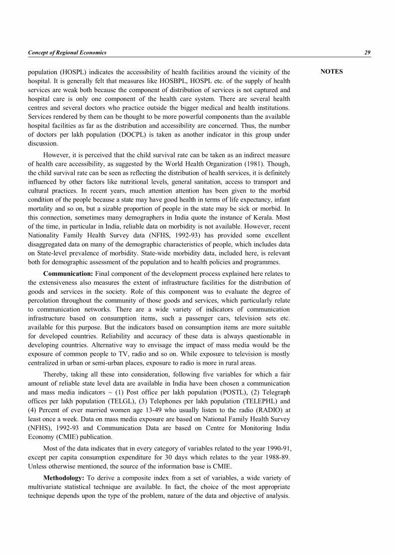
NOTES


population (HOSPL) indicates the accessibility of health facilities around the vicinity of thehospital. It is generally felt that measures like HOSBPL, HOSPL etc. of the supply of healthservices are weak both because the component of distribution of services is not captured andhospital care is only one component of the health care system. There are several healthcentres and several doctors who practice outside the bigger medical and health institutions.Services rendered by them can be thought to be more powerful components than the availablehospital facilities as far as the distribution and accessibility are concerned. Thus, the numberof doctors per lakh population (DOCPL) is taken as another indicator in this group underdiscussion.

However, it is perceived that the child survival rate can be taken as an indirect measureof health care accessibility, as suggested by the World Health Organization (1981). Though,the child survival rate can be seen as reflecting the distribution of health services, it is definitelyinfluenced by other factors like nutritional levels, general sanitation, access to transport andcultural practices. In recent years, much attention attention has been given to the morbidcondition of the people because a state may have good health in terms of life expectancy, infantmortality and so on, but a sizable proportion of people in the state may be sick or morbid. Inthis connection, sometimes many demographers in India quote the instance of Kerala. Mostof the time, in particular in India, reliable data on morbidity is not available. However, recentNationality Family Health Survey data (NFHS, 1992-93) has provided some excellentdisaggregated data on many of the demographic characteristics of people, which includes dataon State-level prevalence of morbidity. State-wide morbidity data, included here, is relevantboth for demographic assessment of the population and to health policies and programmes.

Communication: Final component of the development process explained here relates tothe extensiveness also measures the extent of infrastructure facilities for the distribution ofgoods and services in the society. Role of this component was to evaluate the degree ofpercolation throughout the community of those goods and services, which particularly relateto communication networks. There are a wide variety of indicators of communicationinfrastructure based on consumption items, such a passenger cars, television sets etc.available for this purpose. But the indicators based on consumption items are more suitablefor developed countries. Reliability and accuracy of these data is always questionable indeveloping countries. Alternative way to envisage the impact of mass media would be theexposure of common people to TV, radio and so on. While exposure to television is mostlycentralized in urban or semi-urban places, exposure to radio is more in rural areas.

Thereby, taking all these into consideration, following five variables for which a fairamount of reliable state level data are available in India have been chosen a communicationand mass media indicators ~ (1) Post office per lakh population (POSTL), (2) Telegraphoffices per lakh population (TELGL), (3) Telephones per lakh population (TELEPHL) and(4) Percent of ever married women age 13-49 who usually listen to the radio (RADIO) atleast once a week. Data on mass media exposure are based on National Family Health Survey(NFHS), 1992-93 and Communication Data are based on Centre for Monitoring IndiaEconomy (CMIE) publication.

Most of the data indicates that in every category of variables related to the year 1990-91,except per capita consumption expenditure for 30 days which relates to the year 1988-89.Unless otherwise mentioned, the source of the information base is CMIE.

Methodology: To derive a composite index from a set of variables, a wide variety ofmultivariate statistical technique are available. In fact, the choice of the most appropriatetechnique depends upon the type of the problem, nature of the data and objective of analysis.

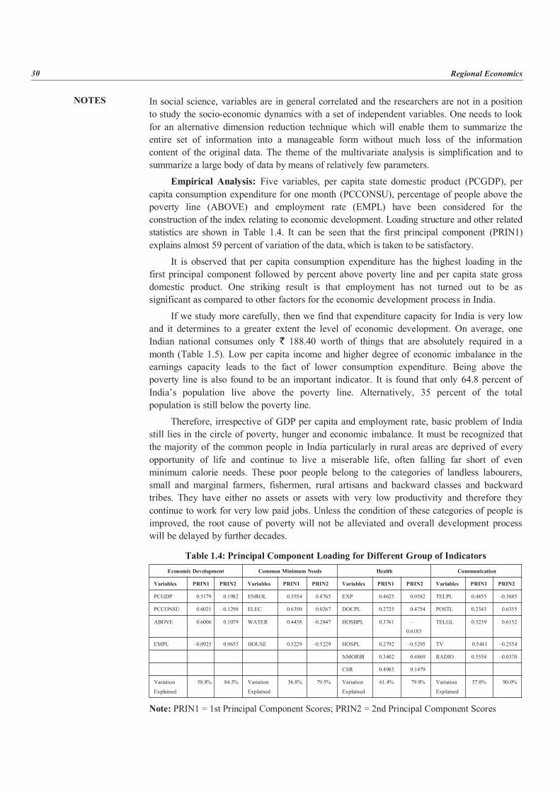
NOTES


In social science, variables are in general correlated and the researchers are not in a positionto study the socio-economic dynamics with a set of independent variables. One needs to lookfor an alternative dimension reduction technique which will enable them to summarize theentire set of information into a manageable form without much loss of the informationcontent of the original data. The theme of the multivariate analysis is simplification and tosummarize a large body of data by means of relatively few parameters.

Empirical Analysis: Five variables, per capita state domestic product (PCGDP), percapita consumption expenditure for one month (PCCONSU), percentage of people above thepoverty line (ABOVE) and employment rate (EMPL) have been considered for theconstruction of the index relating to economic development. Loading structure and other relatedstatistics are shown in Table 1.4. It can be seen that the first principal component (PRIN1)explains almost 59 percent of variation of the data, which is taken to be satisfactory.

It is observed that per capita consumption expenditure has the highest loading in thefirst principal component followed by percent above poverty line and per capita state grossdomestic product. One striking result is that employment has not turned out to be assignificant as compared to other factors for the economic development process in India.

If we study more carefully, then we find that expenditure capacity for India is very lowand it determines to a greater extent the level of economic development. On average, oneIndian national consumes only ` 188.40 worth of things that are absolutely required in amonth (Table 1.5). Low per capita income and higher degree of economic imbalance in theearnings capacity leads to the fact of lower consumption expenditure. Being above thepoverty line is also found to be an important indicator. It is found that only 64.8 percent ofIndia’s population live above the poverty line. Alternatively, 35 percent of the totalpopulation is still below the poverty line.

Therefore, irrespective of GDP per capita and employment rate, basic problem of Indiastill lies in the circle of poverty, hunger and economic imbalance. It must be recognized thatthe majority of the common people in India particularly in rural areas are deprived of everyopportunity of life and continue to live a miserable life, often falling far short of evenminimum calorie needs. These poor people belong to the categories of landless labourers,small and marginal farmers, fishermen, rural artisans and backward classes and backwardtribes. They have either no assets or assets with very low productivity and therefore theycontinue to work for very low paid jobs. Unless the condition of these categories of people isimproved, the root cause of poverty will not be alleviated and overall development processwill be delayed by further decades.

Table 1.4: Principal Component Loading for Different Group of IndicatorsEconomic Development Common Minimum Needs Health Communication

Variables PRIN1 PRIN2 Variables PRIN1 PRIN2 Variables PRIN1 PRIN2 Variables PRIN1 PRIN2

PCGDP 0.5179 0.1982 ENROL 0.3554 0.8765 EXP 0.4625 0.0582 TELPL 0.4855 –0.3885

PCCONSU 0.6021 –0.1298 ELEC 0.6350 0.0267 DOCPL 0.2725 0.4754 POSTL 0.2343 0.6355

ABOVE 0.6006 0.1079 WATER 0.4438 –0.2847 HOSBPL 0.3761 –0.6183

TELGL 0.3239 0.6152

EMPL –0.0925 0.9655 HOUSE 0.5229 –0.5229 HOSPL 0.2792 –0.5295 TV 0.5441 –0.2554

NMORBI 0.3402 0.4869 RADIO 0.5554 –0.0370

CSR 0.4985 0.1479

Variation

Explained

58.8% 84.5% Variation

Explained


Explained


Explained

57.0% 90.0%

Note: PRIN1 = 1st Principal Component Scores; PRIN2 = 2nd Principal Component Scores

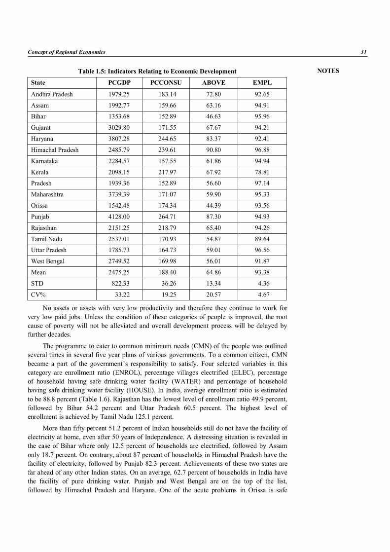
NOTES


Table 1.5: Indicators Relating to Economic Development

State PCGDP PCCONSU ABOVE EMPL

Andhra Pradesh 1979.25 183.14 72.80 92.65

Assam 1992.77 159.66 63.16 94.91

Bihar 1353.68 152.89 46.63 95.96

Gujarat 3029.80 171.55 67.67 94.21

Haryana 3807.28 244.65 83.37 92.41

Himachal Pradesh 2485.79 239.61 90.80 96.88

Karnataka 2284.57 157.55 61.86 94.94

Kerala 2098.15 217.97 67.92 78.81

Pradesh 1939.36 152.89 56.60 97.14

Maharashtra 3739.39 171.07 59.90 95.33

Orissa 1542.48 174.34 44.39 93.56

Punjab 4128.00 264.71 87.30 94.93

Rajasthan 2151.25 218.79 65.40 94.26

Tamil Nadu 2537.01 170.93 54.87 89.64

Uttar Pradesh 1785.73 164.73 59.01 96.56

West Bengal 2749.52 169.98 56.01 91.87

Mean 2475.25 188.40 64.86 93.38

STD 822.33 36.26 13.34 4.36

CV% 33.22 19.25 20.57 4.67

No assets or assets with very low productivity and therefore they continue to work forvery low paid jobs. Unless the condition of these categories of people is improved, the rootcause of poverty will not be alleviated and overall development process will be delayed byfurther decades.

The programme to cater to common minimum needs (CMN) of the people was outlinedseveral times in several five year plans of various governments. To a common citizen, CMNbecame a part of the government’s responsibility to satisfy. Four selected variables in thiscategory are enrollment ratio (ENROL), percentage villages electrified (ELEC), percentageof household having safe drinking water facility (WATER) and percentage of householdhaving safe drinking water facility (HOUSE). In India, average enrollment ratio is estimatedto be 88.8 percent (Table 1.6). Rajasthan has the lowest level of enrollment ratio 49.9 percent,followed by Bihar 54.2 percent and Uttar Pradesh 60.5 percent. The highest level ofenrollment is achieved by Tamil Nadu 125.1 percent.

More than fifty percent 51.2 percent of Indian households still do not have the facility ofelectricity at home, even after 50 years of Independence. A distressing situation is revealed inthe case of Bihar where only 12.5 percent of households are electrified, followed by Assamonly 18.7 percent. On contrary, about 87 percent of households in Himachal Pradesh have thefacility of electricity, followed by Punjab 82.3 percent. Achievements of these two states arefar ahead of any other Indian states. On an average, 62.7 percent of households in India havethe facility of pure drinking water. Punjab and West Bengal are on the top of the list,followed by Himachal Pradesh and Haryana. One of the acute problems in Orissa is safe

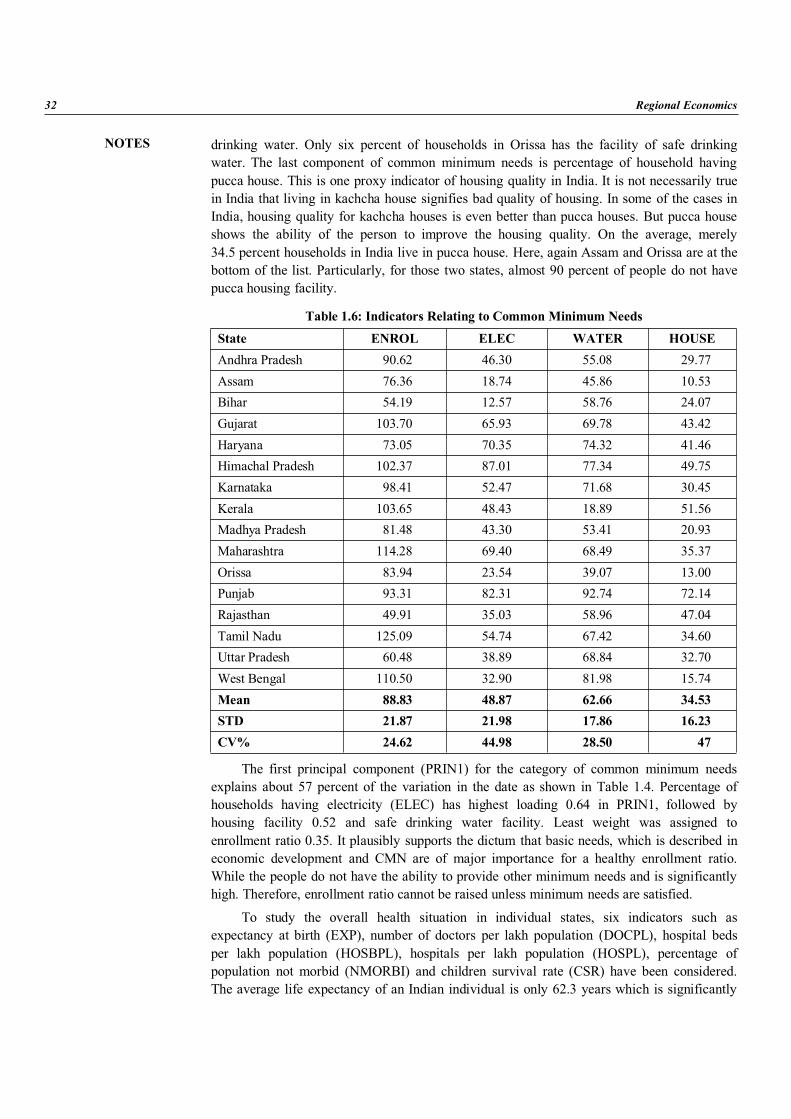
NOTES


drinking water. Only six percent of households in Orissa has the facility of safe drinkingwater. The last component of common minimum needs is percentage of household havingpucca house. This is one proxy indicator of housing quality in India. It is not necessarily truein India that living in kachcha house signifies bad quality of housing. In some of the cases inIndia, housing quality for kachcha houses is even better than pucca houses. But pucca houseshows the ability of the person to improve the housing quality. On the average, merely34.5 percent households in India live in pucca house. Here, again Assam and Orissa are at thebottom of the list. Particularly, for those two states, almost 90 percent of people do not havepucca housing facility.

Table 1.6: Indicators Relating to Common Minimum Needs

State ENROL ELEC WATER HOUSEAndhra Pradesh 90.62 46.30 55.08 29.77Assam 76.36 18.74 45.86 10.53Bihar 54.19 12.57 58.76 24.07Gujarat 103.70 65.93 69.78 43.42Haryana 73.05 70.35 74.32 41.46Himachal Pradesh 102.37 87.01 77.34 49.75Karnataka 98.41 52.47 71.68 30.45Kerala 103.65 48.43 18.89 51.56Madhya Pradesh 81.48 43.30 53.41 20.93Maharashtra 114.28 69.40 68.49 35.37Orissa 83.94 23.54 39.07 13.00Punjab 93.31 82.31 92.74 72.14Rajasthan 49.91 35.03 58.96 47.04Tamil Nadu 125.09 54.74 67.42 34.60Uttar Pradesh 60.48 38.89 68.84 32.70West Bengal 110.50 32.90 81.98 15.74Mean 88.83 48.87 62.66 34.53STD 21.87 21.98 17.86 16.23CV% 24.62 44.98 28.50 47

The first principal component (PRIN1) for the category of common minimum needsexplains about 57 percent of the variation in the date as shown in Table 1.4. Percentage ofhouseholds having electricity (ELEC) has highest loading 0.64 in PRIN1, followed byhousing facility 0.52 and safe drinking water facility. Least weight was assigned toenrollment ratio 0.35. It plausibly supports the dictum that basic needs, which is described ineconomic development and CMN are of major importance for a healthy enrollment ratio.While the people do not have the ability to provide other minimum needs and is significantlyhigh. Therefore, enrollment ratio cannot be raised unless minimum needs are satisfied.

To study the overall health situation in individual states, six indicators such asexpectancy at birth (EXP), number of doctors per lakh population (DOCPL), hospital bedsper lakh population (HOSBPL), hospitals per lakh population (HOSPL), percentage ofpopulation not morbid (NMORBI) and children survival rate (CSR) have been considered.The average life expectancy of an Indian individual is only 62.3 years which is significantly

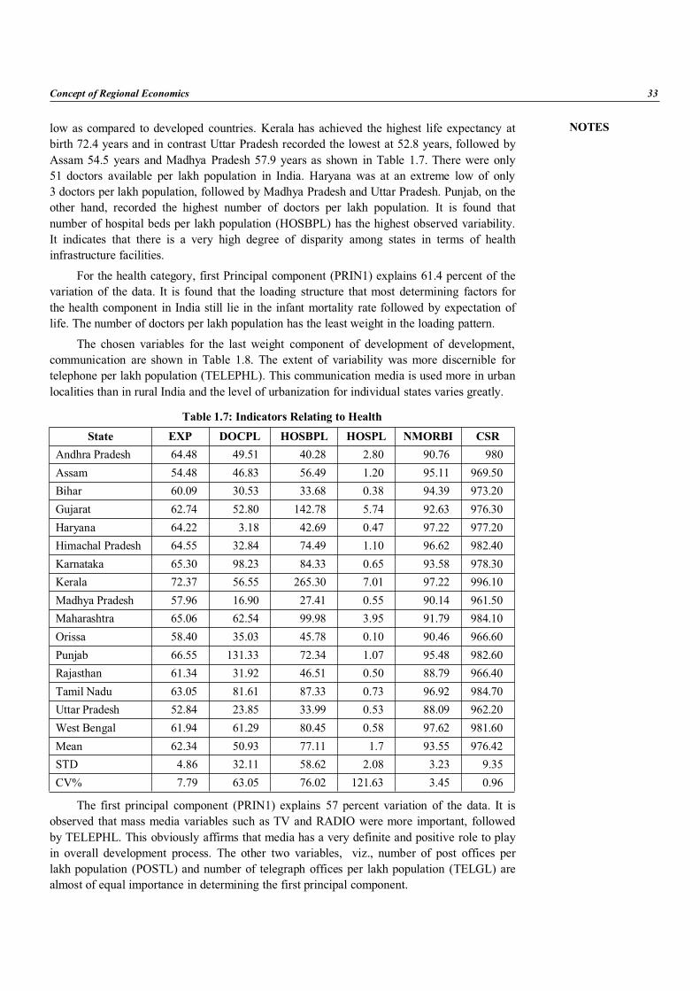
NOTES


low as compared to developed countries. Kerala has achieved the highest life expectancy atbirth 72.4 years and in contrast Uttar Pradesh recorded the lowest at 52.8 years, followed byAssam 54.5 years and Madhya Pradesh 57.9 years as shown in Table 1.7. There were only51 doctors available per lakh population in India. Haryana was at an extreme low of only3 doctors per lakh population, followed by Madhya Pradesh and Uttar Pradesh. Punjab, on theother hand, recorded the highest number of doctors per lakh population. It is found thatnumber of hospital beds per lakh population (HOSBPL) has the highest observed variability.It indicates that there is a very high degree of disparity among states in terms of healthinfrastructure facilities.

For the health category, first Principal component (PRIN1) explains 61.4 percent of thevariation of the data. It is found that the loading structure that most determining factors forthe health component in India still lie in the infant mortality rate followed by expectation oflife. The number of doctors per lakh population has the least weight in the loading pattern.

The chosen variables for the last weight component of development of development,communication are shown in Table 1.8. The extent of variability was more discernible fortelephone per lakh population (TELEPHL). This communication media is used more in urbanlocalities than in rural India and the level of urbanization for individual states varies greatly.

Table 1.7: Indicators Relating to Health

State EXP DOCPL HOSBPL HOSPL NMORBI CSRAndhra Pradesh 64.48 49.51 40.28 2.80 90.76 980Assam 54.48 46.83 56.49 1.20 95.11 969.50Bihar 60.09 30.53 33.68 0.38 94.39 973.20Gujarat 62.74 52.80 142.78 5.74 92.63 976.30Haryana 64.22 3.18 42.69 0.47 97.22 977.20Himachal Pradesh 64.55 32.84 74.49 1.10 96.62 982.40Karnataka 65.30 98.23 84.33 0.65 93.58 978.30Kerala 72.37 56.55 265.30 7.01 97.22 996.10Madhya Pradesh 57.96 16.90 27.41 0.55 90.14 961.50Maharashtra 65.06 62.54 99.98 3.95 91.79 984.10Orissa 58.40 35.03 45.78 0.10 90.46 966.60Punjab 66.55 131.33 72.34 1.07 95.48 982.60Rajasthan 61.34 31.92 46.51 0.50 88.79 966.40Tamil Nadu 63.05 81.61 87.33 0.73 96.92 984.70Uttar Pradesh 52.84 23.85 33.99 0.53 88.09 962.20West Bengal 61.94 61.29 80.45 0.58 97.62 981.60Mean 62.34 50.93 77.11 1.7 93.55 976.42STD 4.86 32.11 58.62 2.08 3.23 9.35CV% 7.79 63.05 76.02 121.63 3.45 0.96

The first principal component (PRIN1) explains 57 percent variation of the data. It isobserved that mass media variables such as TV and RADIO were more important, followedby TELEPHL. This obviously affirms that media has a very definite and positive role to playin overall development process. The other two variables, viz., number of post offices perlakh population (POSTL) and number of telegraph offices per lakh population (TELGL) arealmost of equal importance in determining the first principal component.

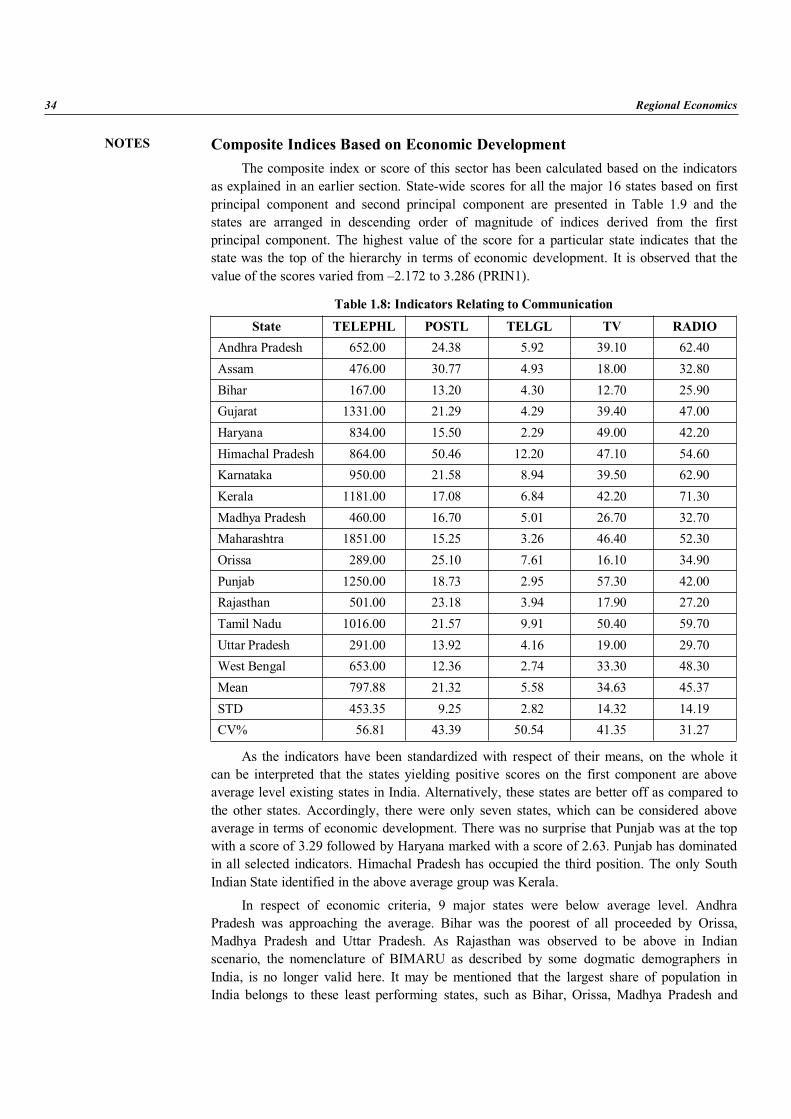
NOTES


Composite Indices Based on Economic DevelopmentThe composite index or score of this sector has been calculated based on the indicators

as explained in an earlier section. State-wide scores for all the major 16 states based on firstprincipal component and second principal component are presented in Table 1.9 and thestates are arranged in descending order of magnitude of indices derived from the firstprincipal component. The highest value of the score for a particular state indicates that thestate was the top of the hierarchy in terms of economic development. It is observed that thevalue of the scores varied from –2.172 to 3.286 (PRIN1).

Table 1.8: Indicators Relating to Communication

State TELEPHL POSTL TELGL TV RADIOAndhra Pradesh 652.00 24.38 5.92 39.10 62.40Assam 476.00 30.77 4.93 18.00 32.80Bihar 167.00 13.20 4.30 12.70 25.90Gujarat 1331.00 21.29 4.29 39.40 47.00Haryana 834.00 15.50 2.29 49.00 42.20Himachal Pradesh 864.00 50.46 12.20 47.10 54.60Karnataka 950.00 21.58 8.94 39.50 62.90Kerala 1181.00 17.08 6.84 42.20 71.30Madhya Pradesh 460.00 16.70 5.01 26.70 32.70Maharashtra 1851.00 15.25 3.26 46.40 52.30Orissa 289.00 25.10 7.61 16.10 34.90Punjab 1250.00 18.73 2.95 57.30 42.00Rajasthan 501.00 23.18 3.94 17.90 27.20Tamil Nadu 1016.00 21.57 9.91 50.40 59.70Uttar Pradesh 291.00 13.92 4.16 19.00 29.70West Bengal 653.00 12.36 2.74 33.30 48.30Mean 797.88 21.32 5.58 34.63 45.37STD 453.35 9.25 2.82 14.32 14.19CV% 56.81 43.39 50.54 41.35 31.27

As the indicators have been standardized with respect of their means, on the whole itcan be interpreted that the states yielding positive scores on the first component are aboveaverage level existing states in India. Alternatively, these states are better off as compared tothe other states. Accordingly, there were only seven states, which can be considered aboveaverage in terms of economic development. There was no surprise that Punjab was at the topwith a score of 3.29 followed by Haryana marked with a score of 2.63. Punjab has dominatedin all selected indicators. Himachal Pradesh has occupied the third position. The only SouthIndian State identified in the above average group was Kerala.

In respect of economic criteria, 9 major states were below average level. AndhraPradesh was approaching the average. Bihar was the poorest of all proceeded by Orissa,Madhya Pradesh and Uttar Pradesh. As Rajasthan was observed to be above in Indianscenario, the nomenclature of BIMARU as described by some dogmatic demographers inIndia, is no longer valid here. It may be mentioned that the largest share of population inIndia belongs to these least performing states, such as Bihar, Orissa, Madhya Pradesh and

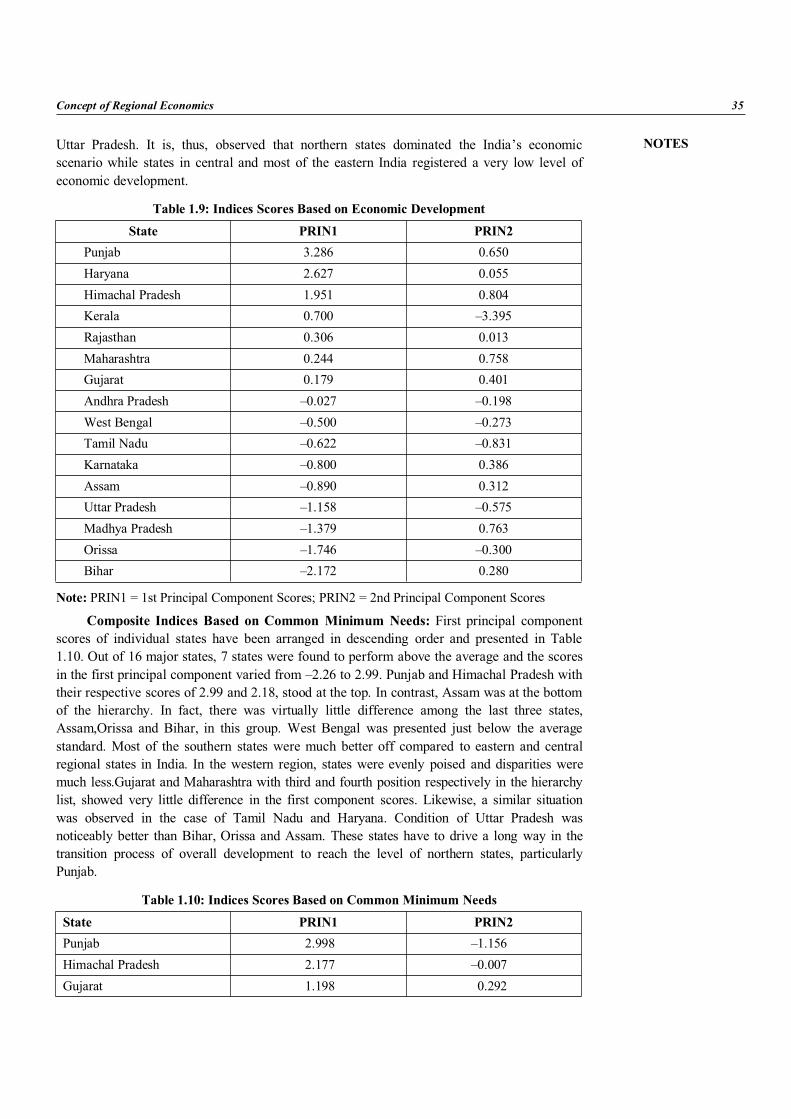
NOTES


Uttar Pradesh. It is, thus, observed that northern states dominated the India’s economicscenario while states in central and most of the eastern India registered a very low level ofeconomic development.

Table 1.9: Indices Scores Based on Economic Development

State PRIN1 PRIN2Punjab 3.286 0.650Haryana 2.627 0.055Himachal Pradesh 1.951 0.804Kerala 0.700 –3.395Rajasthan 0.306 0.013Maharashtra 0.244 0.758Gujarat 0.179 0.401Andhra Pradesh –0.027 –0.198West Bengal –0.500 –0.273Tamil Nadu –0.622 –0.831Karnataka –0.800 0.386Assam –0.890 0.312Uttar Pradesh –1.158 –0.575Madhya Pradesh –1.379 0.763Orissa –1.746 –0.300Bihar –2.172 0.280


Composite Indices Based on Common Minimum Needs: First principal componentscores of individual states have been arranged in descending order and presented in Table1.10. Out of 16 major states, 7 states were found to perform above the average and the scoresin the first principal component varied from –2.26 to 2.99. Punjab and Himachal Pradesh withtheir respective scores of 2.99 and 2.18, stood at the top. In contrast, Assam was at the bottomof the hierarchy. In fact, there was virtually little difference among the last three states,Assam,Orissa and Bihar, in this group. West Bengal was presented just below the averagestandard. Most of the southern states were much better off compared to eastern and centralregional states in India. In the western region, states were evenly poised and disparities weremuch less.Gujarat and Maharashtra with third and fourth position respectively in the hierarchylist, showed very little difference in the first component scores. Likewise, a similar situationwas observed in the case of Tamil Nadu and Haryana. Condition of Uttar Pradesh wasnoticeably better than Bihar, Orissa and Assam. These states have to drive a long way in thetransition process of overall development to reach the level of northern states, particularlyPunjab.

Table 1.10: Indices Scores Based on Common Minimum Needs

State PRIN1 PRIN2Punjab 2.998 –1.156Himachal Pradesh 2.177 –0.007Gujarat 1.198 0.292

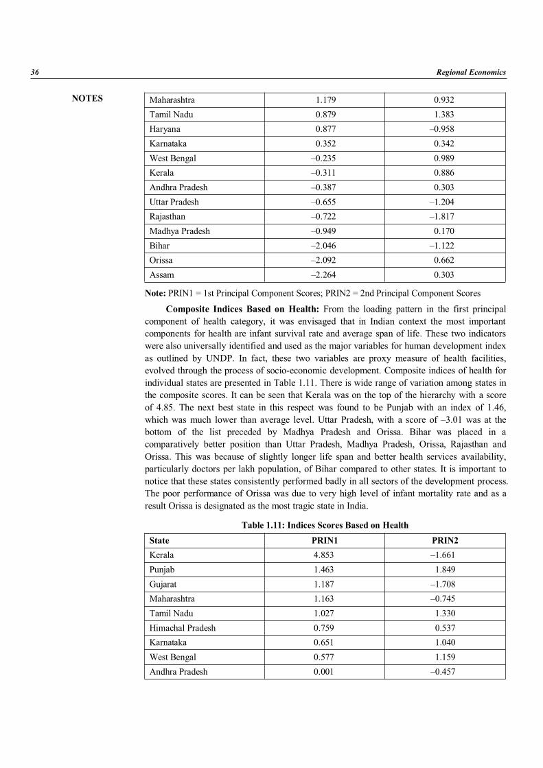
NOTES


Maharashtra 1.179 0.932Tamil Nadu 0.879 1.383Haryana 0.877 –0.958Karnataka 0.352 0.342West Bengal –0.235 0.989Kerala –0.311 0.886Andhra Pradesh –0.387 0.303Uttar Pradesh –0.655 –1.204Rajasthan –0.722 –1.817Madhya Pradesh –0.949 0.170Bihar –2.046 –1.122Orissa –2.092 0.662Assam –2.264 0.303


Composite Indices Based on Health: From the loading pattern in the first principalcomponent of health category, it was envisaged that in Indian context the most importantcomponents for health are infant survival rate and average span of life. These two indicatorswere also universally identified and used as the major variables for human development indexas outlined by UNDP. In fact, these two variables are proxy measure of health facilities,evolved through the process of socio-economic development. Composite indices of health forindividual states are presented in Table 1.11. There is wide range of variation among states inthe composite scores. It can be seen that Kerala was on the top of the hierarchy with a scoreof 4.85. The next best state in this respect was found to be Punjab with an index of 1.46,which was much lower than average level. Uttar Pradesh, with a score of –3.01 was at thebottom of the list preceded by Madhya Pradesh and Orissa. Bihar was placed in acomparatively better position than Uttar Pradesh, Madhya Pradesh, Orissa, Rajasthan andOrissa. This was because of slightly longer life span and better health services availability,particularly doctors per lakh population, of Bihar compared to other states. It is important tonotice that these states consistently performed badly in all sectors of the development process.The poor performance of Orissa was due to very high level of infant mortality rate and as aresult Orissa is designated as the most tragic state in India.

Table 1.11: Indices Scores Based on Health

State PRIN1 PRIN2Kerala 4.853 –1.661Punjab 1.463 1.849Gujarat 1.187 –1.708Maharashtra 1.163 –0.745Tamil Nadu 1.027 1.330Himachal Pradesh 0.759 0.537Karnataka 0.651 1.040West Bengal 0.577 1.159Andhra Pradesh 0.001 –0.457

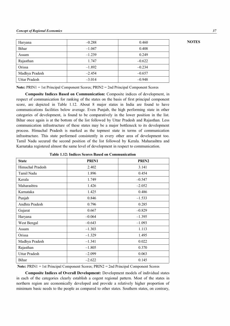
NOTES


Haryana –0.288 0.460Bihar –1.047 0.408Assam –1.239 0.249Rajasthan 1.747 –0.622Orissa –1.892 –0.234Madhya Pradesh –2.454 –0.657Uttar Pradesh –3.014 –0.948


Composite Indices Based on Communication: Composite indices of development, inrespect of communication for ranking of the states on the basis of first principal componentscore, are depicted in Table 1.12. About 8 major states in India are found to havecommunications facilities below average. Even Punjab, the high performing state in othercategories of development, is found to be comparatively in the lower position in the list.Bihar once again is at the bottom of the list followed by Uttar Pradesh and Rajasthan. Lesscommunication infrastructure of these states may be a major bottleneck to its developmentprocess. Himachal Pradesh is marked as the topmost state in terms of communicationinfrastructure. This state performed consistently in every other area of development too.Tamil Nadu secured the second position of the list followed by Kerala. Maharashtra andKarnataka registered almost the same level of development in respect to communication.

Table 1.12: Indices Scores Based on Communication

State PRIN1 PRIN2Himachal Pradesh 2.402 3.141Tamil Nadu 1.896 0.454Kerala 1.749 –0.547Maharashtra 1.426 –2.052Karnataka 1.425 0.486Punjab 0.846 –1.533Andhra Pradesh 0.796 0.285Gujarat 0.667 –0.829Haryana –0.064 –1.395West Bengal –0.643 –1.093Assam –1.303 1.113Orissa –1.329 1.495Madhya Pradesh –1.341 0.022Rajasthan –1.805 0.370Uttar Pradesh –2.099 0.063Bihar –2.622 0.145Note: PRIN1 = 1st Principal Component Scores; PRIN2 = 2nd Principal Component Scores

Composite Indices of Overall Development: Development models of individual statesin each of the categories clearly establish a cogent regional pattern. Most of the states innorthern region are economically developed and provide a relatively higher proportion ofminimum basic needs to the people as compared to other states. Southern states, on contrary,

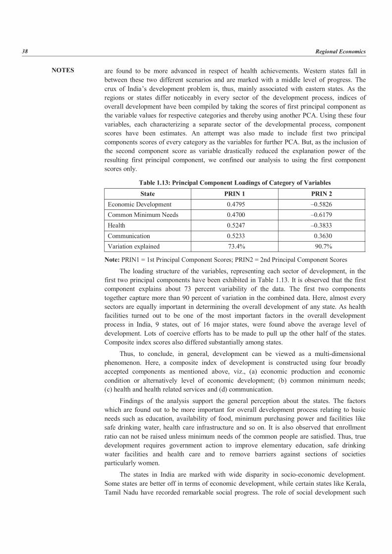
NOTES


are found to be more advanced in respect of health achievements. Western states fall inbetween these two different scenarios and are marked with a middle level of progress. Thecrux of India’s development problem is, thus, mainly associated with eastern states. As theregions or states differ noticeably in every sector of the development process, indices ofoverall development have been compiled by taking the scores of first principal component asthe variable values for respective categories and thereby using another PCA. Using these fourvariables, each characterizing a separate sector of the developmental process, componentscores have been estimates. An attempt was also made to include first two principalcomponents scores of every category as the variables for further PCA. But, as the inclusion ofthe second component score as variable drastically reduced the explanation power of theresulting first principal component, we confined our analysis to using the first componentscores only.

Table 1.13: Principal Component Loadings of Category of Variables

State PRIN 1 PRIN 2Economic Development 0.4795 –0.5826Common Minimum Needs 0.4700 –0.6179Health 0.5247 –0.3833Communication 0.5233 0.3630Variation explained 73.4% 90.7%


The loading structure of the variables, representing each sector of development, in thefirst two principal components have been exhibited in Table 1.13. It is observed that the firstcomponent explains about 73 percent variability of the data. The first two componentstogether capture more than 90 percent of variation in the combined data. Here, almost everysectors are equally important in determining the overall development of any state. As healthfacilities turned out to be one of the most important factors in the overall developmentprocess in India, 9 states, out of 16 major states, were found above the average level ofdevelopment. Lots of coercive efforts has to be made to pull up the other half of the states.Composite index scores also differed substantially among states.

Thus, to conclude, in general, development can be viewed as a multi-dimensionalphenomenon. Here, a composite index of development is constructed using four broadlyaccepted components as mentioned above, viz., (a) economic production and economiccondition or alternatively level of economic development; (b) common minimum needs;(c) health and health related services and (d) communication.

Findings of the analysis support the general perception about the states. The factorswhich are found out to be more important for overall development process relating to basicneeds such as education, availability of food, minimum purchasing power and facilities likesafe drinking water, health care infrastructure and so on. It is also observed that enrollmentratio can not be raised unless minimum needs of the common people are satisfied. Thus, truedevelopment requires government action to improve elementary education, safe drinkingwater facilities and health care and to remove barriers against sections of societiesparticularly women.

The states in India are marked with wide disparity in socio-economic development.Some states are better off in terms of economic development, while certain states like Kerala,Tamil Nadu have recorded remarkable social progress. The role of social development such

NOTES


as literacy and more particularly female literacy to promote basic capabilities emerges as theprerequisite to overall development. Entitlements to basic commodities and services alsovaries significantly among states. These results emphasize the role of well functioning publicactions in improving the overall living conditions of the people. The disparity in entitlementof basic necessities among states mainly emanates from the scope and quality of a wide rangeof public services like schooling facilities, basic health care and public food distributionsystem. Indeed, Kerala’s success may be attributed to the role of public action to promote arange of social opportunities relates to elementary education, status of women in society andprovisions for health care and other services. The condition of BOUMAR states, on contraryis the result of incessant public neglect of the same opportunities. Therefore, the overall resultof incessant public neglect of the same opportunities. Hence, the overall results evidentlyshows that economic reforms alone are not adequate for overall development unless it isaccompanied by social and political commitments. Faster development necessitatesgovernment action to improve elementary education, particularly for the younger generation.Kerala has set up the instance and has clearly progressed. It has a sluggish economy and ahigh level of unemployment. Though economic growth in the sense of expanding grossnational product and other related variables is one of the most fundamental input to theoverall development process, the basic objective of development should focus on theexpansion of human capabilities which has been neglected for too long in India.

1.4 SUMMARY

1. Blair (1995) attempts to separates economic growth from development.2. Regional and local economics is a study of political economy.3. Main theories that underpin the analysis are rooted in the various political economy

schools of thought like interventionist (Mainstream or Keynesian); free market(Conservative or Monetarist); and Marxist.

4. Fundamentally, the regional and local economy is all economic activity takingplace in a specific geographically defined area.

5. Regional analysis is mostly based on the theories and analytical tools developed fornational economies.

1.5 SELF ASSESSMENT QUESTIONS

I. Fill in the Blanks1. Government departments work through ________ and it co-ordinates the work of

other government departments in ________.2. Models are based on the ________ that similar sorts of ________.

II. True and False1. National governments and policy makers are able to exercise a degree of control

over external trade.2. In the region, income is largely determined by what happens outside the region,

e.g., government spending, taxation, national wage rates etc.

NOTES


III. Multiple Choice Questions1. Barriers to trade are missing at the local level. It implies ________.

(a) Distance to market is shorter – transportation costs (lower)(b) Labour and capital are more mobile within the region than between countries(c) There are no defence or political considerations(d) All of the above

2. A composite index based on several indicators has been developed using principalcomponent analysis and states are arranged according to the indices derived usingfour broadly accepted components ________.(a) Economic production and economic condition or alternatively level of

economic development(b) Common minimum needs(c) Health and health-related services(d) Communication(e) All of the above

Short Answer Questions1. Explain in brief about the tools used in regional analysis.2. Define Econometric Models and Cost Benefit Analysis.

Long Answer Questions1. Explain in detail about the ‘importance of regional analysis in developed and

backward economies’ in the Indian context.2. Critically analyze the strategy of the Socio-economic Development in India.

1.6 KEY TERMS

DemographicImmiserizationInterventionistMainstreamRegression analysis

1.7 KEY TO CHECK YOUR ANSWER

I. 1. regional offices, every region, 2. assumption, fundamental components.II. 1. True, 2. True.

III. 1. (d), 2. (e).

2Chapter


Definitional problems in regions: (a) Physical or Geographical, (b) Demographic(c) Planning regions and, (d) Model Regions (analysis for identification of a region)Regional approach to the problems of backward economy.

Structure:2.1 Definitional Problems in Regions: (a) Physical or Geographical, (b) Demographic

(c) Planning Regions and (d) Model Regions (Analysis for Identification of a Region)2.2 Regional Approach to the Problems of Backward Economy2.3 Summary2.4 Self Assessment Questions2.5 Key Terms2.6 Key to Check your Answer

2.1 DEFINITIONAL PROBLEMS IN REGIONS: (A) PHYSICAL ORGEOGRAPHICAL, (B) DEMOGRAPHIC (C) PLANNING REGIONSAND (D) MODEL REGIONS (ANALYSIS FOR IDENTIFICATIONOF A REGION)

Definitional Problems in Regions

(a) Physical or Geographical:Defining Regions: With the end of the Cold War and the trend towards economic

globalization as well as the increasing complexity of international relations, the conceptregion risks becoming an empty idea. These forces have redefined the structural and agentiverelationships between the global, regional and national contexts. Moreover, they are leadingus to re-examine the theoretical foundations of the study of regionalism. Our regional imagesare often based on unexamined and outdated metageographical conceptions of the world — aperspective dubbed the ‘‘jigsawpuzzle view’’ that assumes discrete, sharply bounded, staticcontinental units fit together in an unambiguous way. Yet, the world is not structured in sucha neat manner; to the contrary, regions disappear and reappear as they are transformed byvarious economic, political, and cultural factors.

STRATEGIES TO DEALWITHREGIONAL ANALYSIS

NOTES


Key Distinctions: Often those engaged in defining the concept region are content to listphysical, political and economic criteria without embarking on theory development. Forinstance, Edward Mansfield and Helen Milner emphasize geographical proximity andspecificity as the key defining traits of a region. Further, researchers refer to early conceptualanalyses and essentially leave the concept undefined. Scholars in history and political scienceseem to think that they will know a region when they see one. For economists, the choice iseven easier, region is coextensive with a preferential trading agreement or a customs union.

Therefore, L. Alan Winters explains in detail the concept of multilateralism but takes itscounterpart, regionalism, almost for granted. For him, it refers to any policy designed toreduce trade barriers between a sub-set of countries, regardless of whether those countries areactually contiguous or even close to each other.

These are inadequate solutions to the definitional problem because both the character andfunctions of regions have recently experienced a major transformation. One change hasoccurred in the relative weights given various levels of analysis — global, regional, nationaland the links between them. During the Cold War, most regions were either political ormercantile clusters of neighbouring countries that had a place in the larger international system.Occasionally, political and military motives fostered the establishment of super regions such asthe North Atlantic Treaty Organization (NATO) and the Organization of African Unity (OAU).

However, since the late 1980s, sub-regional and micro-regional organizations havebecome more common, for example, the Baltic Council of Ministers, the Visegrad Group, theShanghai Group, and Mercosur. This trend is, in part, a response to the fragmentation ofgreat-power blocs, especially in Eastern Europe and Central Asia, but it also reflects the needto react to the pressures created by economic globalization through local means.

A second change is the growing differentiation between physical (geographical andstrategic) regions and functional (economic, environmental, and cultural) regions. Thistransformation appears linked to the first change. Increasing emphasis on the global-regionalrelationship has led to paying more attention to functional and subregional relations, eventhough the nation-region nexus is still predominantly viewed in physical and State-centric terms.

Distinction between physical and functional regions is reminiscent of Manuel Castellsdifferentiation between a space of places and a space of flows. He defined a place as a localewhose form, function and meaning are self-contained within the boundaries of physicalcontiguity. Places are historically rooted yet reshaped increasingly by the flows ofinformation and people. The space of flows refers to the ‘material organization of the time-sharing social practices that work through flows and networks’.

A number of scholars have tried to link the physical and functional conceptions ofregions by focusing on the boundary-eroding consequences of globalization and identityformation and the extra-territorial challenges to sovereignty that these forces unleash. Theysuggest that physical and functional definitions of regions may be viewed as a sequence inwhich territory gradually gives way to space. Indeed, the transition from physical tofunctional regionalism is due to the increase in the interaction capacity of the system. In alow-capacity international system, physical vicinity matters; states are linked with theirneighbours by economic and security concerns and international relations are subsystemdominant. An increase in the interaction capacity of the system helps the actors reach beyondtheir immediate neighbourhoods; these new contacts give rise to more system-dominantinternational relations.

NOTES

Strategies to Deal with Regional Analysis 43

Regionalism and the End of the Cold War: During the Cold War, bipolarity andnuclear weapons created contextual effects that contributed to the emergence of a semi-globalsystem. In Europe, in particular, extended US nuclear deterrence and Soviet political-militarycontrol of its eastern half limited the autonomy of individual states and made them parts of alarger whole. Local security systems existed, but they were overshadowed by the ability ofexternal powers to move directly into the local security complex with the effect ofsuppressing the indigenous security dynamic. The end of the Cold War has reduced theeffects of the global system on regional security dynamics and national decisions. Thus, anend to the bipolar cleavage has led to a restoration of regional sovereignty and to theestablishment of several regional powers dominating their geographical areas .

Changes in the international structure and new security challenges were expected topush the development of regionalism, providing order and stability in the regions andcertainly in Africa, the Middle East and Southeast Asia, one can discern tendencies toward adiminution in the presence of the major powers, especially the USSR. Indeed, Arthur Steinand Steven Lobell have argued that even during the Cold War, regional security was notglobalized. Though the United States was a significant player in most regional securityarrangements, it, too, remained reluctant to participate in African and Asian conflicts thatwere not considered central to its interests.

In the post-Cold War international system, even though there has been an increasingdemand for external intervention and crisis management for humanitarian and other politicalreasons, neither the United States nor any other major power has shown a willingness toshoulder the full responsibility for managing these regional crises. As a solution to thisdilemma, some have suggested the establishment of a concert of powers to replace globalhegemony which is thought to be unattainable and a balance-of-power system which isconsidered unstable. Indeed, a central theme of David Lake and Patrick Morgan’s book‘Regional Orders’ is the advocacy of regional concerts and the assessment of their feasibility.

Globalization and Regionalization: In the security sphere, the weakness of globalarrangements has given priority to the national and regional levels and as major powers,particularly the United States, wield decisive unilateral and multilateral influence, thenational-regional linkage continues to dominate international security relations. If concertsbetween major powers are established at all, they are informal arrangements focusing on themanagement of a particular crisis rather than, as traditional theories suggest, comprehensivearrangements to produce collective security. The Contact Group, dealing originally withBosnia and then other parts of the former Yugoslavia, is an instance of a new type of concertof major powers.

In the economic sphere, however, the situation is quite different. The process ofglobalization, although partial and variable in nature, is creating an increasingly autonomouseconomic reality that interacts directly with both national and regional economies. Theformation of regions takes place at the interface between global economic and technologicalforces and national realities. National actors may, in fact, perceive regionalism as a defensemechanism against the competitive pressures arising from the globalization process.Moreover, regions are shaped by the spillover of domestic conditions across borders. Despitethat connection, the new regionalism cannot be linked solely with national factors andseparated from the global context. Instead, the two processes of globalization andregionalization are articulated within the same larger process of global structural change.

The mutual interdependence or dialectic between globalization and regionalization iswidely accepted; indeed, among radical political economists the point is uncontested.

NOTES


According to Samir Amin, the historical development of capitalism has been to graduallymove from the local level to the global, and at each step to create new polarizing tendencies.To be able to improve their economic positions, peripheral countries have had to delinkthemselves from the global system and adopt alternative, countervailing strategies, one ofwhich is regionalization. James Mittelman also considers ‘transformative regionalism acounterthrust to neoliberal globalization. His view of regionalism is more nuanced thanAmin’s noting that the tendency toward flexible specialization in global production networksgives rise to many different types of regional and transborder arrangements. Mittelman warnsagainst a too strict contrast between globalization and regionalism. This point has been mademore specifically by Ralph Pettman who reminds us that such a simple dichotomy has bothanalytical and political costs. Analytically, one may ask what’s the point of dichotomizingregionalism and globalism when they would seem to be points along a continuum and notreally opposed? Politically, the counterposing of these two categories can lead to anantagonistic impression that the West is global and the East regional.

Relationship between globalization and regionalization has been extensively studied anddebated by mainstream economists. The basic question underlying this research and currentdebates is stated well by Bhagwati when he asks – Were the preferential free trade areas andcustoms unions belonging to the second regionalism of the 1980s building blocs or stumblingblocs for the multilateral economic order? In his view, due to the dominating effects of tradediversion, regionalism became a stumbling bloc, slowing down progress toward multilateralism.

One of the few exceptions is Robert Lawrence who argues that economic globalizationdoes, in fact, demand deeper regional integration. He rejects the traditional view that foreigndirect investment (FDI) and trade are substitutes for each other. Instead, Lawrence observesthe growing role of FDI and the need it creates to restructure, specialize, and engage innetwork production. The expansion of FDI has led to regional production and service clustersintended to improve efficiency and reduce transaction costs. Due to the globalization of FDI,regional integration has become progressively deeper and moved beyond preferential tradingarrangements.

Political-Military Regions: Given our discussion to this point concerning global-regional security linkages, especially from the viewpoint of concert theory, it is possible toconclude not only that this linkage is relatively weak but that the theory itself is conceptuallymuddled and empirically of limited value. Therefore, alternative formulations are needed tocreate a proper spatial context for security theories. This task seems all the more importantbecause defining region and regionalism using the concepts of traditional security theoriesdoes not appear to be of much help. Neorealism – with its focus on anarchy, risks of defection,and relative gains – does not take spatial dimensions seriously. The same applies to neoliberalinstitutionalism in which spatial concepts find hardly any place at all. Instead, institutions aretreated almost exclusively as analytical and non-spatial phenomena. Only in discussions ofoffensive realism do we find strong geopolitical undertones as a result of its concentration ongreat-power competition.

Externalities: The problematic status of regionalism in mainstream internationalrelations theories may explain why their supporters introduce the spatial dimension onlyindirectly by using general concepts such as externalities. An illustrative externality is theconcept regional security complex, defined as a group of states whose primary securityconcerns link sufficiently closely that their national securities cannot realistically beconsidered apart from one another. These complexes are kept together by the negative orpositive security links between states.

NOTES


The externality approach does not address the conceptual transition from the study ofregional systems to regional orders that is a common weakness in the theory of regionalsecurity complexes. In fact, the approach seems to lead to the study of coalition formation asthe operative mechanism in region formation, reinforced by the emphasis on transaction costs.One can assume that actors use externalities as grounds for making decisions on theirparticipation in regional security arrangements. Furthermore, it seems likely that actorsaffected by the same external effects are inclined to deepen their co-operation for mutualprotection. The traditional example is, of course, the establishment of a defensive coalitionagainst a common external threat. This reaction tends to exclude sources of negativeexternalities from the regional system. Against this backdrop, one can define a regionalsecurity system as a coalition in which positive externalities are maximized and negativeexternalities minimized. This choice helps give size and a spatial domain to the regionalsystem. This theory of externalities can help us differentiate among security orders.Integration and the building of security communities are principal intra-regional strategiesthat facilitate the development of a local security order, but hegemony, concert, and balanceof power almost always involve extra-regional powers. As it may be misleading to excludeexternal factors from the analysis of regional security, a potential next step would be toexplore the relationship between the intra- and extra-regional dimensions of security orders.Such an analysis would benefit from the specification of the kinds of externalities thatdifferent security orders produce, for instance, the externalities of hegemony (limitation ofthe domestic autonomy of smaller states) compared with those involved in the balance ofpower (breakdowns that can lead to war).

Functional Regionalism

Social Spaces: The social definition of region focuses on functional exchanges as thesource of spatiality and can be traced back to Jean Gottman’s distinction betweeniconography and circulation, between places and flows to use today’s terminology. Anothermajor contributor to the definition of spatiality was Robert Sack who distinguished betweenterritoriality used to control a spatial political organization and non-territorial action; heconsidered territoriality as the attempt to affect, influence or have control over a specific area.Later on, Sack realized that territory is usually contested and started to stress the importanceof access to it. The distribution of territorial power is rarely equitable because actors havedifferent abilities to control and enter a particular territory. With this in mind, Sack redefinedterritoriality as a “strategy to establish differential access to people, things, and relationships”.

Economic Regions: Economic regionalization appears to depend on both politicaldecisions at the regional level and the locational decisions made by firms. In effect, regionsare viewed as an appropriate unit in which to organize governance and stimulate politicalparticipation. But often, as in the European Union, regional governance has remained weak.In fact, its regional dimension has been more manifest in the rise of economic pivot regionsand of capital- and technology-intensive cities that support local development. There isevidence to suggest that, at least in Europe, differences in regional growth rates havedepended on a combination of local conditions and their linkages to the world economy.Neither the state nor regional government alone can assure regional success that is based onthe interrelationship among local resources, transnational capital, and public-privateinteractions. Loose policy initiatives and regional networks cannot save a regional project ifits market incentives are inadequate.

Regional specialization and growth are due both to expanding trade and investment aswell as endogenous factors. Decreasing transaction costs play a role in the relocation of

NOTES


production within and between countries. The result is a center-periphery division thatchanges as development spurts integrate new regions into the center. Due to backward andforward linkages, production tends to agglomerate to areas where there is already similarproduction, irrespective of the intensity of trade relations.

(b) Demographic:The term Demography implies – studies of a population based on factors such as age,

race, sex, economic status, level of education, income level and employment, among others.Demographics are used by governments, corporations and non-government organizations tolearn more about a population’s characteristics for many purposes, including policydevelopment and economic market research. Demographic trends are also important, as thesize of different demographic groups will change over time as a result of economic, culturaland political circumstances.

Health

Maternal Health in India: India continues to contribute about a quarter of all globalmaternal deaths. WHO defines maternal mortality as the death of a woman during pregnancyor in the first 42 days after the birth of the child due to causes directly or indirectly linkedwith pregnancy.

Fast Facts: Globally, every year over 500,000 women die of pregnancy related causesand 99 percent of these occur in developing countries. The Maternal Mortality Ratio (MMR)in India is 254 per 100,000 live births according to Sample Registration System (SRS) Reportfor 2004-2006. This is a decline from the earlier ratio of 301 during 2001-2003. MMR in Chinastands at 45, Sri Lanka at 58, Bangladesh at 570, Nepal at 830 and Pakistan at 320 in 2006.

Wide disparities exist across states in India. The MMR ranges from 95 in Kerala to 480in Assam.

UNICEF in Action: Building on the achievements of the Government of India’sNational Rural Health Mission (NRHM), UNICEF continues to support health programmessuch as the Village Health and Nutrition Days (VHND), to reach out to pregnant women inunderserved areas, ensuring that they receive the three essential antenatal check-ups andsensitizing them about the importance of institutional deliveries. UNICEF is working closelywith National Rural Health Mission programmes such as Janani Suraksha Yojana toencourage women to have institutional deliveries.UNICEF follows the continuum of careapproach to ensure that both mother and newborn receive necessary services. This involves achain of interventions that begin with complete and comprehensive antenatal care, increasingskilled attendance at birth, ensuring that first referral units are equipped to deal withemergency obstetric care and ensuring that both the mother and newborn are followed up postpartum.

Neonatal Health in India: Child mortality is a sensitive indicator of a country’sdevelopment. In India, the Infant Mortality Rate (IMR) (under one year) has shown a modestdecline in recent years. The average decline of IMR per year between the years 2004 to 2008has been about 1 percent per year. In 2008, the IMR was 53/1,000 live births. Eight statescontribute to 75 per cent of infant mortality: Uttar Pradesh, Bihar, Madhya Pradesh,Rajasthan, Andhra Pradesh, Orissa, Gujarat and Assam. At the current rate of decline, Indiawill miss the XI Plan goal of reduction in IMR and the Millennium Development Goal-4 onchild survival. About 70 percent of the childhood under-five is caused by perinatal conditions

NOTES


(33.1 percent), respiratory infections (22 percent) and diarrhea (13.8 percent). Malnutrition isan underlying cause responsible for about one-third of all deaths in childhood.

Fast Facts: Averting neonatal deaths is pivotal to reducing child mortality. TheNewborn period is the period starting from birth and continues throughout 28 days of life.Neonatal mortality rate (mortality in the newborn period) stands at 35/1000 lives births, andcontributes to 65 percent of all deaths in the first year of life.

Between 2004-2008, neonatal mortality has moved from 37/1000 live births to 35/1000 only.

56 percent of all newborn deaths occur in five states: Uttar Pradesh, Rajasthan, Orissa,Madhya Pradesh and Andhra Pradesh.

Three major causes contribute to about 60 percent of all deaths in the newborn period:pre-maturity and low birth weight, birth asphyxia and infections.

UNICEF in Action: UNICEF partners with the Government of India, stategovernments and communities, promote simple interventions which can significantlyimprove newborn survival. UNICEF encourages home-based care of all newborns through itssupport to the Integrated Management of Newborn and Childhood Illness (IMNCI)programme. The programme equips frontline workers with the required skills and supplies.Following training on IMNCI, frontline workers (ASHAs and AWWs) visit newborns at theirhouseholds three times in the first week of life. During the visits, the workers assess thenewborns, promote healthy practices, manage simple problems and refer those with seriousillnesses. UNICEF supports intensive behaviour change communication efforts through allchannels to promote key practices that improve survival of newborns. UNICEF raisesawareness of media and elected representatives on issues related to newborn and childsurvival. UNICEF supports setting up and managing of Special Care Newborn Units (SCNUs)that provide state-of-the-art care for newborns in some of the least developed districts of thecountry.

Measles in India: The respiratory disease measles remains a leading cause of deathamong young children, despite the fact that a safe and effective vaccine has been available for40 years. Measles is an acute illness caused by a virus of the paramyxo virus family. It is oneof the most contagious diseases and many children who do not have sufficient immunitycontract measles if exposed. During the first few weeks after contracting measles, a child’simmune system becomes weakened, and a normal cold or diarrhoea can become a lifethreatening illness.

UNICEF/WHO Actions: The global reduction in death from measles reflects support andcommitment by the Measles Initiative to boosting immunization coverage and by nationalgovernments to following the World Health Organization (WHO)/UNICEF comprehensivestrategy for reducing measles mortality. This strategy consists of four key components:

1. Providing at least one dose of measles vaccine at routine vaccination coverage of atleast 90 per cent of children, administered at nine months of age.

2. Giving all children a second opportunity for measles vaccination.3. Establishing effective surveillance.4. Improving clinical management of complicated cases – including Vitamin A

supplementation

India Celebrates Victory over Polio: Completing three full years without reportingany case of polio, India celebrated a landmark achievement in public health on 11 February2014 – the victory over polio. India has not reported any case of polio since a two-year old

NOTES


girl got polio paralysis on 13 January 2011 in Howrah district of West Bengal. India’s victoryover polio paves the way for polio-free certification of the Southeast Asia region of WHO inMarch end. This is an unprecedented progress for a country, which reported more than halfthe global polio cases until the year 2009. Experts always predicted India would be the last tostop polio as its endemic pockets in parts of Uttar Pradesh and Bihar were among the mostdifficult places in the world for polio eradication. India overcame huge challenges, with astrong commitment that matched $2 billion allocation over the years to stop polio.Implementing innovative strategies, the programme reaches an incredible 99 percentcoverage in polio campaigns, ensuring every child, even in the remotest corner of the countryis protected against polio.

India introduced the oral polio vaccine in 1985 in the Universal ImmunizationProgramme in the backdrop of over 200,000 cases of polio annually (as per estimates of theIndian Academy of Pediatrics). In 1995, the first national polio immunization campaign washeld; since then two national and multiple sub-national campaigns are rolled out every yearfor children up to 5 years of age. In each national polio campaign, 2.3 million lakhvaccinators, led by 155,000 supervisors, visit 209 million households to immunize 170 millionchildren up to the age of 5 years.

Nutrition: The level of child undernutrition remains unacceptable throughout the world,with 90 percent of the developing world’s chronically undernourished (stunted) childrenliving in Asia and Africa.

Detrimental and often undetected until severe, undernutrition undermines the survival,growth and development of children and women, and diminishes the strength and capacity ofnations. With persistently high levels of undernutrition in the developing world, vitalopportunities to save millions of lives are being lost, and many more millions of children arenot growing and developing to their full potential.

Nutrition is a core pillar of human development and concrete, large-scale programmingnot only can reduce the burden of undernutrition and deprivation in countries but also canadvance the progress of nations.

UNICEF ActionUNICEF supports the Government in its objectives to reduce and prevent malnutrition,

and to improve the development of children under three-years old, especially those inmarginalized groups. UNICEF is assisting the government to further expand and enhance thequality of ICDS in various ways: by improving the training of anganwadi workers; bydeveloping innovative communication approaches with mothers; helping to improvemonitoring and reporting systems; providing essential supplies; and by developingcommunity based early childcare interventions. UNICEF supports iron supplementation foradolescent girls and Vitamin A supplementation for children. It encourages the universal useof adequately iodized salt by educating the general population and collaborating with the saltindustry. UNICEF’s programme contributes to reducing hunger and malnutrition rates,especially among the three most vulnerable groups of children (0-35 months old), children ofeconomically disadvantaged populations and children of socially excluded groups.

Water, Environment and Sanitation: UNICEF’s long standing support for improvingwater supply, sanitation and hygiene stems from a firm conviction and based on soundevidence that these are central to ensuring the rights of children. In fact, it is essential forchildren to survive, grow and develop into healthy and fulfilled citizens of the world. In the

NOTES


broader context, UNICEF’s activities in Water, Sanitation and Hygiene (WASH) contributeto the achievement of the Millennium Development Goals.

Sanitation: It is estimated that only 31 percent of India’s population use improvedsanitation (2008).

In rural India, 21 percent use improved sanitation facilities (2008).One hundred forty-five million people in rural India gained access to improved

sanitation between 1990-2008.

Two hundred and eleven million people gained access to improved sanitation in wholeof India between 1990-2008. India is home to 594 million people defecating in the open; over50 percent of the population.

In Bangladesh and Brazil, only seven percent of the population defecate in the open. InChina, only four percent of the population defecate in the open.

Water: 88 percent of the population of 1.2 billion has access to drinking water fromimproved sources in 2008, as compared to 68 percent in 1990. Only a quarter the totalpopulation in India has drinking water on their premise.

Women, who have to collect the drinking water, are vulnerable to a number of unsafepractices. Only 13 per cent of adult males collect water. Sixty-seven percent of Indianhouseholds do not treat their drinking water, even though it could be chemically or bacteriallycontaminated.

Hygiene: According to the Public Health Association, only 53 percent of the populationwash hands with soap after defecation, 38 percent wash hands with soap before eating andonly 30 percent wash hands with soap before preparing food. Only 11 percent of the Indianrural families dispose child stools safely. 80 percent children’s stools are left in the open orthrown into the garbage. Only 6 percent of rural children less than five years of age usetoilets. Wash interventions significantly reduce diarrhoeal morbidity; statistically, it has beenshown that:

1. Handwashing with soap reduces it by 44 percent.2. Household water treatment by 39 percent.3. Sanitation by 36 percent.4. Water supply by 23 percent.5. Source water treatment by 11 percent.Key Issues:

1. Newborn infants: Handwashing by birth attendants before delivery has beenshown to reduce mortality rates by 19 percent while a 4 percent reduction in riskof death was found if mothers washed their hands prior to handling theirnewborns.

2. Children under five years: Poor wash causes diarrhoea, which is the secondbiggest cause of death in children under five years. Diarrhoea is an immediatecause of undernutrition.

3. School-aged children: Children prefer to attend schools having adequate andprivate wash facilities. Schools provide an excellent opportunity for children tolearn about hygiene practices.

4. Older girls: Giving girls the knowledge and facilities necessary for goodmenstrual hygiene is key to their dignity, their privacy, their educational

NOTES


achievement and their health. Adolescent girls are empowered through improvedmenstrual hygiene management.

5. Mothers and caregivers: Handwashing with soap at critical times is important forprotecting the health of the whole family. By being a role model, mothers andcaregivers can also help instill in their children the good hygiene practices whichwill serve them for life.

6. Children in emergencies: During emergencies, children are especially vulnerableto the effects of inadequate access to water and sanitation services. Wash is a keycomponent of any emergency response.

Chemical contamination in water ensuring water quality at the source is crucial. In India,there is a widespread natural occurrence of arsenic and fluoride in the groundwater. UNICEFis supporting Government of India programmes on arsenic and fluoride mitigation andidentifying water quality testing technologies which are appropriate for use in field situations.All emergencies cause disruption to basic services. People are less likely to be able to drinksafe water, use basic sanitation facilities and maintain improved hygiene practices. Children,especially those under the age of five, are particularly vulnerable to the diseases which canresult during emergencies. These diseases include diarrhoea, cholera, typhoid, respiratoryinfections, skin and eye infections which are all likely to occur when water supplies andsanitation services are disrupted. UNICEF has set out minimum standards of response for anyemergency situation. These describe the life-saving actions which UNICEF will take withinthe first six to eight weeks of an emergency, along with the longer term role in the subsequentweeks and months.

UNICEF Action: UNICEF supports the national and state governments in developingand implementing a range of replicable intervention models for sanitation, hygiene and watersupply. UNICEF’s Childs Environment Programme in India supports the government’sflagship programmes of Total Sanitation Campaign to improve access to and use of sanitationfacilities and the National Rural Drinking Water Programme to provide adequate safe waterto every rural household in India. The Child’s Environment Programme also works withSarva Shiksha Abhiyan and Integrated Child Development Services, to promote hygienewater and sanitation services in schools, anganwadi centers and health centers with lastingoutcomes.

HIV/AIDS: The National AIDS Control Programme (NACP) III 2007-2012 has theoverall goal of halting and reversing the epidemic in India. Over 99 percent of the populationin the country is free from infection. NACP III places highest priority on prevention whileseeking to integrate care, support and treatment for those affected by HIV/AIDS.

Fast Facts: Global, Regional and India Estimates

1. An estimated 33.4 million people worldwide were living with HIV (2008).2. Approximately 2.1 million children under 15 were living with HIV (2007).3. An estimated 2.1 million people died of AIDS-related causes (2007).4. An estimated 290,000 children under 15 died of AIDS-related causes (2007)5. India has a low HIV prevalence of 0.34 percent. Yet in terms of individuals infected,

India is home to the third largest number of people living with HIV in the world.6. The vast majority of HIV infections in India occur through sexual transmission

(85.6 percent).7. Nearly five percent of infections are attributable to parent-to-child transmission.

NOTES


8. The epidemic disproportionately affects women, who account for 40 percent of thetotal infections in the country.

9. In India, the epidemic is more pronounced in urban areas than rural ones anddecreases with increasing education levels.

Key Issues:

The Four Ps: The global and country level response to HIV is based on acomprehensive approach that includes the following four strategic elements, or the four Ps:

1. Preventing HIV transmission from women living with HIV to their infants2. Primary prevention of HIV infection among couples of child bearing age3. Preventing unintended pregnancies among women living with HIV4. Providing appropriate protection to children affected by HIV and their families

Prevention of Parent-to-Child Transmission (PPTCT): In India, the transmission ofthe virus from the mother-to-child during pregnancy, labour and delivery or breastfeeding iscalled parent-to-child-transmission to emphasize the role of the father in both thetransmission of the virus and management of the infected mother and child. Nearly fivepercent of infections are attributable to parent-to-child-transmission. It is estimated that out of27 million pregnancies every year, nearly 49,000 occur in HIV-positive mothers. As ofDecember 2008, only 16 percent of pregnant women were tested for HIV, while 22 percent ofthe children born to the estimated 49,000 HIV-positive women were receiving anti-retroviralprophylaxis. The number of facilities offering HIV testing and counselling went up from4,269 in 2007 to 4,817 in 2008 and stands at 4,987 as of March 2009. In 2009, only 11,489 ofan estimated 49,000 pregnant women living with HIV received anti-retroviral treatment toprevent parent-to-child transmission. This is because of multiple factors including socialcustoms, lack of family support and financial barriers, which constrain women from availingof institutional care necessary for administering treatment. PPTCT services have also notbeen scaled up in remote areas with lower HIV prevalence. One of the best practices inPPTCT in India is the outreach approach, used by the ICTC to ensure that HIV-positivewomen who are tested are followed up before, during and after an institutional delivery, andprovided with anti-retroviral prophylaxis. The core principle of this approach rests on thecontinuum of care for women, children and their families – a chain of interventions that beginbefore pregnancy and continue through pregnancy, labour and delivery and subsequently as partof routine or specialized chronic care services for after the child is born.

Pediatric Care and Treatment: It is estimated that 70,000 children below the age of15 are living with HIV in India and 21,000 children are infected every year through parent-to-child transmission. A small proportion are also infected by unsafe injections and infected byblood transfusions. Most children are infected with the virus while still in the womb, duringbirth. The National Pediatric Anti-retroviral Treatment (ART) Initiative was launched in 2006.A total of 40,000 children living with HIV will be provided ART by the end of NACP III. Atotal of 375 ART centres shall be equipped to offer pediatric ART in the country. Follow-upof HIV exposed infants, according to the Indian Guidelines, begins at six weeks. The Road toHealth Card for these children includes information on maternal HIV status, co-trimoxazoleprophylaxis, infant HIV diagnosis and infant feeding information. To reach more mother-infant pairs, the Reproductive and Child Health (RCH) Programme is linked to the PPTCTand Pediatric HIV Programme in order to provide for and incorporate HIV care into thepackage of services for mothers and children.

NOTES


Preventing Infection among Young Adolescents and Young People: In India, theprevalence of HIV among 15-19 year olds is 0.04 percent and that among 20-24 year olds is0.18 percent. By the end of the NACP III, about 25 million students will have been reachedthrough the Adolescent Education Programme. The NACP III will also bring HIV preventionskills education programmes and related services to 70 million young people who are not inschool, including, street children, children of CSWs, children in institutions, child labourersand other vulnerable youth.

Protection, Care and Support for Children Affected by AIDS: In the short term,NACP III will reach out to as many children living with HIV as possible to provide them withthe treatment and the care and support services that they need. In the long term, NACP IIIaims to ensure that every child has access to the same comprehensive set of basic health,education and social protection services, regardless of their HIV status or that of any memberof their family.

UNICEF in Actions: UNICEF supports the Government in its effort to halt and reversethe HIV/AIDS epidemic in India, and mitigate its impact on affected children and women.UNICEF is assisting the government to further expand and enhance the quality ofprogrammes to reduce the transmission of HIV from infected mothers to their children and toincrease the access of these mothers and their children to treatment in various ways: byproviding strategic supplies of drugs and commodities, improving the capacity of staff; bydeveloping innovative communication approaches for prevention and care; and helping toimprove monitoring and reporting systems. UNICEF supports efforts to reduce stigma anddiscrimination against children and people affected by HIV and for commitment on ensuringtheir equal access to essential health, social welfare and educational services. UNICEF’sprogramme contributes to increasing knowledge, dispelling myths and misconceptionsrelating to HIV transmission and prevention, and behaviours among vulnerable young people.

Child Protection: UNICEF India’s programmatic approach to child protection aims tobuild a protective environment in which children can live and develop in the full respect oftheir fundamental rights. Translated into action, this approach led to a multi-layeredprogramme whose scope is to understand and address the multiple vulnerabilities of childrenin need of special protection rather than tackle only their immediate manifestations. UNICEFChild Protection Programme in India focuses mainly on three areas of intervention: childlabour, child trafficking, and children in difficult circumstances. UNICEF India’sprogrammatic approach to child protection aims to build a protective environment in whichchildren can live.

In the area of Child Labour, projects implemented in various states of the country adoptan essentially holistic approach, combining strategies aimed not only to the withdrawal ofchildren from work, but also to enhance communities’ awareness, ownership and collectiveaction for the protection and promotion of children rights. Existing strategies include:(a) Promotion of education as both, key preventive measure and essential component for therehabilitation of released children; (b) Addressing poverty related factors through thepromotion of self-help groups; (c) Advocacy and social mobilisation for the elimination ofchild labour. In Uttar Pradesh, for instance, this strategy led to an increase of more than47 percent in school enrollment and attendance among the villages targeted by the ongoingUNICEF child labour elimination intervention. Over 120 Alternative Learning Centers (ALC)have been established in order to facilitate mainstreaming of out-of-school children intoformal education and through them more than 24,000 children have been able to go back toschool. Moreover, over 1000 Self-help Groups have been established and they are now

NOTES


playing a crucial role in reducing indebtedness among poor rural families. Women’sempowerment is also showing to be instrumental to the well-being of children as a whole.With the support of UNICEF, for example, 50 percent of targeted villages have adopted threekey-friendly practices, namely an immunization coverage of more than 80 percent, a schoolenrollment rate of more than 90 percent and a sensible increase in the age of marriage. In thearea of child trafficking, UNICEF India supports the Government with a twofold strategyaimed to strengthen rescue mechanisms and reduce at the same time, children’s vulnerabilityto trafficking through a special focus on preventive action. For this purpose, a NationalCommunication Strategy on child trafficking has been developed and is now beingimplemented at community level through UNICEF state offices. Manuals have beendeveloped for social workers, judiciary, and counsellors working on issues of childtrafficking in order to enable rescue and rehabilitation processes which are in the best interestof the child. As a part of its efforts to formulate strategies and legislations on issues related tochild protection, UNICEF also supports the Ministry of Women and Child Development,Government of India, to undertake a national level study on children affected by violence andto conduct regional and national consultations on child marriage and to hold dialogues onOffences against Children Bill. In the efforts to improve the implementation of the JuvenileJustice System in the country, UNICEF is also supporting the government with thedevelopment of training materials for the judiciary and various other functionaries of thesystem like the child welfare committee members, police and care-takers in the variousinstitutions under the Act. UNICEF is also collaborating with the Ministry of Women andChild Development on the creation of a website for Missing Children to facilitate tracing andreintegration of lost children.

Education: The Education Programme supports and strengthens government efforts toprovide quality education by reducing gender and other social and economic disparities at thenational and state levels. The Ministry of Human Resource Development is the nodalministry for UNICEF’s Education Programme.

Through a close and productive partnership with MHRD and the Department of SchoolEducation and Literacy along with civil society, the programme has been supporting theGovernment of India’s flagship programme Sarva Shiksha Abhiyan (Education for All)1 toensure greater access to education, enrollment and improved learning outcomes for the mostmarginalized groups of children. While retaining a focus on elementary education forchildren aged 6-14 years under the Right of Children to Free and Compulsory Education Act(RTE), the programme is now covering a wider gamut – starting from early childhoodeducation through elementary up to Grade 10. Child friendly schools and systems are beingpromoted and capacities of teachers strengthened to ensure children’s right to learn.Convergence with other programmes to combat child labour and child marriage, anduniversal access to improved water, sanitation and hygiene facilities, is also ensured. Theprogramme aims to improve equitable access to quality early childhood education. It includes:

1. Accelerate implementation of the Right to Education Act and child friendly schools2. Enhance capacities of teachers and pre-school functionaries to deliver quality

education3. Mobilize communities to demand equitable access to quality education4. Increase access to secondary education for adolescents with a focus on reducing

gender and social disparities.

NOTES


(c) Planning Regions:Economic and Developmental Challenges in India

Sustainable growth: The United Nations describes sustainable growth as a process thatfulfills the needs of the present without compromising the ability of future generations tomeet their own needs. This year, academics working on India questioned whether Indiangrowth was truly sustainable or whether the country had failed to utilize resources generatedby recent economic growth by investing much more in education and health care anddeveloping infrastructure in an environmentally responsible way. Heading into 2014, Indiamust better assess how to enhance economic growth together with low-carbon developmentinitiatives including ways to improve food and water security.

Inclusive growth: For Indian growth to be sustainable, it must be inclusive to coverissues related to inequalities between castes (including tribal children and elderly peopleliving in remote areas), colour, disability, gender, regions (rural-urban as well as differencesbetween states), and more. While the gender gap in employment and political participationhas been narrowing, there is much more to be done for the health and safety of girls and women.India needs to do more to ensure inclusive growth, particularly by improving social protectionpolicies. Good examples such as ‘Amma’s canteen’, which was recently introduced in TamilNadu and sells highly subsidized nutritious meals, are worth expanding to other states to solveproblems related to high malnutrition levels.

Demographic dividend: Approximately 200 million Indians are between the ages of15 and 24 and India is well positioned to make the most of a growing population of workingage. However, to reap the demographic dividend, India will have to manage the demand andsupply of skills and labour carefully. While the government has introduced policies toimprove access to education, much more needs to be done to improve the quality of education,standards of teaching, methods of examination, development of skills, vocationalprogrammes, etc. In order to make Right to Education policy effective, the country shouldalso address the challenges of bridging the gaps between children from disadvantaged andadvantaged backgrounds being able to study together and better understand, respect andbefriend each other. In the new year, India should look to develop public-private partnershipsand social entrepreneurship programmes that can ensure livelihoods for its young population.

Inflation: The issue of high inflation is uppermost in the minds of politicians,policymakers and the people. Consumer prices in India have risen at an average annual paceof 10 percent during the past five years, and Indian households are bracing for another13 percent increase next year. To check inflation, the Reserve Bank of India has raisedinterest rates and will review India’s monetary policy framework in line withrecommendations by the Urjit Patel Committee, which is expected to submit its report at theend of the year. It is also essential to manage artificially induced national and internationalmechanisms. The Central Bank and Ministry of Finance are working together to analyze andunderstand the reasons and find ways to encourage investment and curb inflation.

Rapid urbanization: Indian cities are growing at an unprecedented rate—the country’surban population is expected to grow to 590 million people by 2030. This rapid urbanizationis also expected to drive economic growth. According to some estimates, cities couldgenerate up to 70 percent of new jobs created until 2030 and produce 70 percent of IndianGDP. To reap the economic advantages of urbanization, the Indian government must developbetter policies to meet urban infrastructure needs through sustainable means and addressgrowing urban poverty and inequality.

NOTES


Land reforms: The Land Acquisition Act passed this year received mixed views. Thereare concerns that the new law will drive up costs across the economy and make severalindustrial and real estate projects unviable, without necessarily delivering justice to farmersand landowners whose lands are acquired. These and other challenges related to landreform – particularly in the context of urbanization and the growing need for low-incomeurban housing – mean that India will have to continue drafting land related legislation toensure sustainable and equitable growth.

Centre-state dynamics: The evident role of states in influencing economic growth,governance and policies has increasingly become more prominent. States are drivinglocalized growth, enhancing their own investments, and developing models that are beingreplicated across the country. But the centre needs to do more to facilitate state-stateinteraction and the states should also be proactive in sharing of knowledge of best practicesamong themselves. The central government should also seek to do more to balancethe uneven growth between states.

Older citizens: While India seeks to harness its young population to drive growth, itmust also start planning for increased expenditure on health and welfare services for theelderly. Fertility rates in India are declining as life expectancy increases. There will be morethan 300 million Indians over the age of 60 by 2050. ‘Indians never seem to retire’ has beensaid of people in various sectors, particularly in urban areas, as many continue to work forseveral years after retirement. Nevertheless, the shifting demographics will add to the burdenof inadequate healthcare, welfare services, and families. Elderly women, who will outnumbermen, are expected to be the most vulnerable. In addition, there are interesting opportunitiesand challenges of elderly parents remaining in India while their children have migrated. Totackle these challenges, India must develop policies to ensure that its older citizens too havehealthy and happy lives.

India-China trade: Despite various diplomatic standoffs this year, the governments ofboth India and China remain eager to boost bilateral trade to US$100 billion in the next fewyears. No doubt, trade with China is a significant component of India’s economy. But traderelations remain one-way, with more Indian consumers buying Chinese goods than the otherway around. India will have to address this trade deficit in the new year by improving itsexport competitiveness and identifying more goods, services and policies to enhancebalanced trade with to China.

India-Pakistan trade: In the past decade, India-Pakistan trade has increased fromUS$370 million per year to US$2.4 billion. But this is just a start. According to some estimates,the volume of a normalized bilateral trade regime could be as high as US$40 billion. The onusfor progress on bilateral trade relations currently rests with Pakistan. Despite repeated calls forimproved India-Pakistan ties, Prime Minister Nawaz Sharif, who was elected to power in May,has yet to grant India Most Favoured Nation status. While there is little India can do to boosttrade until Pakistan takes this key step, New Delhi should continue its support for increasedbilateral trade, as it would be for the benefit of the economies of both India and Pakistan whilealso helping to improve the political relations between the two countries.

(d) Model Regions (Analysis for Identification of a Region):Guidelines for development of Regional Model Competency Standards (RMCS)

Regional Skills and Employability Programme (SKILLS-AP): National skill standardsplay an important and increasing role in vocational training and recognition in the Asia-Pacific region as they do in many other parts of the world. They are a guide to the scope of

NOTES


skills and knowledge required for a whole industry and can be flexibly combined into jobs oroccupations. Skill standards are now the common basis for vocational training programmes,and testing and certification in many countries. This Guideline is for development ofRegional Model Competency Standards (RMCS) that can be used in various ways tounderpin efficient and effective skill development in the Asia-Pacific region.

The future of work is changing: The nature of work is changing rapidly due to newtechnology and work organization innovations. This has a dual effect by tending todramatically reduce the number of low or unskilled positions available globally andadditionally putting emphasis on the need to extend worker’s skills over a shorter and shortertime frame. It is no longer sufficient to only have initial skills in say, a recognized trade as thechanging nature of work will require individuals to regularly upgrade their skills or addcompletely new ones in order to remain fully employable. Most of this upgrading or additionof skills can be gained in a training centre or within the workplace but irrespective of howcompetency has been achieved it should be formally recognized in the same way as the initialtrade skills were. RMCS can provide a flexible benchmark for the whole range of skillsneeded in an industry and so support recognition, upgrade training and certificationirrespective of where or how the skills were gained.

Work or qualification levels across the region: Skill standards developed in differentcountries have levels or hierarchies used to group the skills defined. In the Asia-Pacificregion, these are usually based upon occupational classification structures and the particularqualification framework for that country. However, both of these vary considerably across theAsia-Pacific region and worldwide in terms of the number of occupational definitions, levelsof qualifications and terminology used. For example, common references to concepts such as‘basic’ or ‘advanced’ are used as occupation or qualification descriptors in a number ofcountries but the definition of these terms is not consistent internationally. As most countriesin the region will have a level or classification system for their own particular qualificationsor skill recognition credentials, RMCS must allow for this. So, RMCS do not definequalification levels but rather clusters competencies in logical groupings that can betranslated into each country’s classification system as required. As the movement of labouracross borders increases every year, it is important to have a common translation tool such asRMCS to allow the skills of migrant workers to be evaluated simply no matter whatqualification they hold.

Benefits of Regional Model Competency Standards (RMCS): RMCS are valuablefor the following reasons:

1. Changes in the labour market must be duly reflected in new regional skill standards.The ongoing effects of globalization and technological development have aprofound impact on jobs. The skill requirements for most jobs change rapidly soreflecting these changes and providing a basis for regional co-operation isnecessary.

2. Companies can use regional model competency standards to describe the skillsthey need in a common language. Existing workforces can be evaluated againstmodel standards to determine whether the necessary range of skills and knowledgeis held by workers and where any gaps may be.

3. The approach to describing workplace needs for human resources in competencystandards can accommodate rapid changes in skill requirements, as the process ismore closely linked to the needs of industry than course based learning outcomesand curriculum.

NOTES


4. Previous skill description systems such as Model Occupational Skill Standards(MOSS) used traditional occupations as a basis for clustering competencies.

The new competency-based model standards are designed for broader industry, industrysub-sector or occupational cluster coverage and so have a wider application and are quickerto develop for industry:

(i) where there is migration of skilled workers;(ii) where there is strong economic development; and

(iii) where work is service focussed and not only traditional manufacturing trades.

RMCS are simply developed sets of competency standards in streams of occupational orindustry sector groupings. It is up to users in any particular economy to determine which ofthe standards should make up local qualifications or other recognition tools such as licensing.In most countries that use competency standards across their training system, it has beenfound that whole qualifications are not always the only, or best way to aggregatecompetencies. Increasingly, smaller sets of skills make up highly valued job roles and assistindividual workers not wanting or needing lengthy ‘trade’ style qualifications.

In today’s faster paced world of work, even existing workers with respectedqualifications still need to upgrade frequently to keep abreast of new technologies and workplacepractices. They need to access short, sharp training programmes that put together valuablenew competencies that complement each other. There are also many new portfolio workerswho undertake a variety of jobs across various occupational sectors according to demand.

An industry focus for RMCS: The RMCS concept deals with a whole industry ormajor industry sectors not single occupations. This does not mean, however, that recognizedoccupations, including traditional trades are not covered by RMCS. All the functions andskills to work effectively in an industry or discrete industry sector can be described in acommon, competency based format. To do this, the RMCS format is designed to allowvarious combinations of work functions to be put together to describe whole jobs. Thisapproach can also show combinations of competencies that are the equivalent of existingtrade or other occupations. Well-designed RMCS, therefore, accommodate industry jobrequirements and cross-industry or trade requirements from within the same framework ofdescriptors. In other words, everyone can get something useful from them as a tool for:

(i) describing new jobs for any industry;(ii) designing vocational training or testing materials for all work, including trades;

(iii) conducting skills audits at the enterprise or national level, i.e., for assessing theskills of migrant workers;

(iv) restructuring an enterprise or industry sector for development of new services andmanufactures;

(v) planning for multi-skilling of a workforce; and(vi) introduction of team based approaches to work.

The economic success of any countries’ businesses will be through high value technicalapplication, innovation, customer service, business acumen and enterprise. Workers in theemerging world economy must be more knowledgeable about their industry culture andenterprise needs and utilize this knowledge to contribute to innovation. The correlationshipbetween technical skills, knowledge (technical and vocational), innovation and business/self-management looks like this:

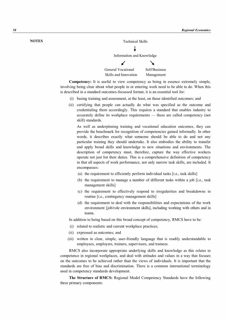
NOTES


Technical Skills

Information and Knowledge

General Vocational Self/BusinessSkills and Innovation Management

Competency: It is useful to view competency as being in essence extremely simple,involving being clear about what people in or entering work need to be able to do. When thisis described in a standard outcomes-focussed format, it is an essential tool for:

(i) basing training and assessment, at the least, on those identified outcomes; and(ii) certifying that people can actually do what was specified as the outcome and

credentialing them accordingly. This requires a standard that enables industry toaccurately define its workplace requirements — these are called competency (notskill) standards.As well as underpinning training and vocational education outcomes, they canprovide the benchmark for recognition of competencies gained informally. In otherwords, it describes exactly what someone should be able to do and not anyparticular training they should undertake. It also embodies the ability to transferand apply broad skills and knowledge to new situations and environments. Thedescription of competency must, therefore, capture the way effective workersoperate not just list their duties. This is a comprehensive definition of competencyin that all aspects of work performance, not only narrow task skills, are included. Itencompasses:(a) the requirement to efficiently perform individual tasks [i.e., task skills](b) the requirement to manage a number of different tasks within a job [i.e., task

management skills](c) the requirement to effectively respond to irregularities and breakdowns in

routine [i.e., contingency management skills](d) the requirement to deal with the responsibilities and expectations of the work

environment [job/role environment skills], including working with others and inteams.

In addition to being based on this broad concept of competency, RMCS have to be:

(i) related to realistic and current workplace practices;(ii) expressed as outcomes; and

(iii) written in clear, simple, user-friendly language that is readily understandable toemployees, employers, trainers, supervisors, and trainees.

RMCS also incorporate appropriate underlying skills and knowledge as this relates tocompetence in regional workplaces, and deal with attitudes and values in a way that focuseson the outcomes to be achieved rather than the views of individuals. It is important that thestandards are free of bias and discrimination. There is a common international terminologyused in competency standards development.

The Structure of RMCS: Regional Model Competency Standards have the followingthree primary components:

NOTES


1. Industry Descriptor and Coverage2. Primary Functions3. Units

The third component – Units – are structured with four sub-components:

Performance CriteriaEvidence requirementsCritical Skills and Essential KnowledgeRange Statement

Let’s look at each component and sub-component in turn with examples of how they areused and drafted.

Industry Descriptor and Coverage: A Regional Model Competency Standard for say,the air-conditioning industry might include the following information in its description andcoverage statement:

The intention of this opening RMCS statement is to describe succinctly and clearly whatthe whole set of model standards covers in industry or industry sector terms. It is importantnot to simply go to occupational descriptions because one industry may use skills from manyoccupations and, conversely, occupations can cross a number of different industries. Thedescriptor and coverage needs careful consideration because it defines the parameters of themodel standards being developed and sets the boundaries of the skills defined.

Primary Functions: Continuing with this example of an RMCS Industry, descriptionand coverage, one of the primary functions for our air-conditioning industry could be:

Primary Function: Install, test and commission domestic air-conditioning systems.This is a broad range of work that occurs after specifications for an air-conditioning systemhave been determined. The system has been built or acquired and is now ready for installation.It would be broken down into a number of different actions and each will require a range ofskills to be used. This is where the RMCS Unit structure comes in.

Units: Again using the above example of a Primary Function in Air-conditioninginstallation, some of the relevant Units could be:

1. Planning work to meet all requirements of installation drawings and technicalspecifications;

2. Installing with minimal structural displacement, to a clean finish and withinrelevant building codes of practice;

3. Connecting the system to domestic power supply in a safe manner which meetsapplicable electrical regulations;

4. Testing and adjusting system to ensure flow rates, noise levels, and filtering meetsystem specifications and customer requirements;

5. Commission system and hand over to customer with appropriate warrantydocumentation, operating instructions and maintenance schedules accuratelycompleted and explained.

Performance Criteria: The first example Unit above would have a number ofPerformance Criteria describing real work outcomes. They are drafted to describe in detailthe skills a worker applies when undertaking the work defined in the Unit. While quiteconcise, they must set out fully what is done, how well the work should be performed and

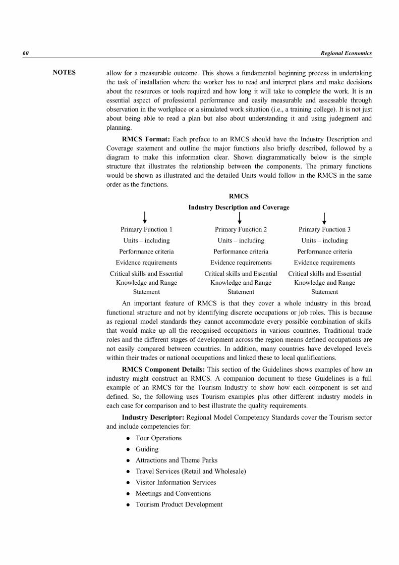
NOTES


allow for a measurable outcome. This shows a fundamental beginning process in undertakingthe task of installation where the worker has to read and interpret plans and make decisionsabout the resources or tools required and how long it will take to complete the work. It is anessential aspect of professional performance and easily measurable and assessable throughobservation in the workplace or a simulated work situation (i.e., a training college). It is not justabout being able to read a plan but also about understanding it and using judegment andplanning.

RMCS Format: Each preface to an RMCS should have the Industry Description andCoverage statement and outline the major functions also briefly described, followed by adiagram to make this information clear. Shown diagrammatically below is the simplestructure that illustrates the relationship between the components. The primary functionswould be shown as illustrated and the detailed Units would follow in the RMCS in the sameorder as the functions.

RMCSIndustry Description and Coverage

Primary Function 1 Primary Function 2 Primary Function 3Units – including Units – including Units – including

Performance criteria Performance criteria Performance criteriaEvidence requirements Evidence requirements Evidence requirements

Critical skills and Essential Critical skills and Essential Critical skills and EssentialKnowledge and Range Knowledge and Range Knowledge and Range

Statement Statement Statement

An important feature of RMCS is that they cover a whole industry in this broad,functional structure and not by identifying discrete occupations or job roles. This is becauseas regional model standards they cannot accommodate every possible combination of skillsthat would make up all the recognised occupations in various countries. Traditional traderoles and the different stages of development across the region means defined occupations arenot easily compared between countries. In addition, many countries have developed levelswithin their trades or national occupations and linked these to local qualifications.

RMCS Component Details: This section of the Guidelines shows examples of how anindustry might construct an RMCS. A companion document to these Guidelines is a fullexample of an RMCS for the Tourism Industry to show how each component is set anddefined. So, the following uses Tourism examples plus other different industry models ineach case for comparison and to best illustrate the quality requirements.

Industry Descriptor: Regional Model Competency Standards cover the Tourism sectorand include competencies for:

Tour OperationsGuidingAttractions and Theme ParksTravel Services (Retail and Wholesale)Visitor Information ServicesMeetings and ConventionsTourism Product Development

NOTES


The scope of the standards is for entry level to middle management and encompassescommon sector skills in the areas of customer relations, tourism product development, salesand bookings, travel and tour operations and tourist attractions. There is also inclusionthroughout of competencies that are not exclusive to the Tourism industry but are commonskills that could apply to many different workplaces. These include:

Customer ServiceHygiene, Health, Safety and SecurityGeneral AdministrationFinancial AdministrationComputer TechnologyTechnical and Maintenance ServicesMerchandise SalesTrainingManagement and Leadership.

Primary Functions: Every RMCS will have a number of primary functions. How manyof these are there depends upon the particular industry or occupational cluster covered by theRMCS. Each primary function describes the major type of work involved – administrative,technical and so on with a range of contexts for its application. Careful construction of theprimary functions is necessary as they determine the utility of the whole RMCS. This is themajor difference between defining a set of model standards for an industry or a similarexercise for an occupation. Occupations are definitions of sets of skills with broaddescriptions of how they are applied but they do not easily show what skills are brought tobear in any particular industry or enterprise. Working from what occurs in an industry allowsall the work functions to be defined not just those covered in traditional trades or well-knownjobs. It shows how work interrelates across an industry and what the full range of skillsnecessary are.

Units: RMCS should provide the basis for skill formation now, and in the future.Capturing the ability to apply skills in new situations and changing work organization ratherthan only reflecting the tasks currently performed. Each primary function has a number ofUnits describing the work in more detail. These are statements about what particular work isdone – utilizing certain technology or materials, working with others or alone, operatingwithin certain regulatory requirements and so on – and the performance measures that applyto a competent worker. It is vital that these are in outcome terms and do not simply describe aprocess or input. Each begins with a brief statement of what the Unit covers. As industriesdevelop RMCS, it is important to pinpoint current and likely changes, and identify the skillrequirements emerging from these in the coverage statement. It is one of the most vitalaspects of making model standards really useful and ‘futureproof’.

Performance Criteria: Performance criteria are evaluative statements in a Unit whichspecify what is to be done in the work environment and the required level of performance. Itis here that the activities, skills, knowledge and understanding which provide the evidence ofcompetent performance, are specified as outcomes within the Unit. Considering the followingprinciples and examples will support development of good performance criteria. Breadth andprecision in expression is essential.

Evidence: The next component of the RMCS is guidance on the sort of evidence thatwould support an assessment process and determine if an individual really held the

NOTES


competencies described. Evidence covers the sort of broad activities that should be observedor simulated in an assessment to reliably attest to a person being able to apply a competencyin a realistic workplace environment and include the modes of evidence that are best for thecompetency:

(i) direct observation for some units;(ii) written or oral testing for others; or

(iii) evaluation of longer term work or practice outcomes such as complete products,service records and so on.

An RMCS Evidence requirement needs to provide information on the ways in whichcompetency can be reliably determined – as previously noted, it is particularly important tocover aspects of work that are not easily observable in routine situations. In the TourismRMCS, one of the primary functions covers tour guiding. A Unit might deal with guiding agroup of tourists in remote or potential hazardous situations. An Evidence statement might,therefore, be required which ensures a trainer or assessor evaluates whether the potential tourguide understands the safety and environmental aspects of guiding their clients.

Critical Skills and Essential Knowledge: Skills and knowledge are integrated into allcompetency standards although how this is done can vary. The practical skills to bedemonstrated in an occupation or job are best interwoven into the performance criteria ratherthan separately referred to but a list of what might be termed ‘critical’ skills can be noted.Using our Tourism RMCS, a Primary Function component is promoting and attractingtourists to events such as sporting tournaments, concerts and so on. A Unit dealing withcommunicating with clients to ascertain their needs in this regard would have Critical Skillaspects to be assessed.

Critical applications of competency might also include having sufficient theoreticalknowledge to source alternative options/strategies, based on the evidence, i.e., problemsolving skills including knowledge of some broad process. This is illustrated in a competencyfrom an RMCS for Automotive Service and Repair dealing with the technical skill ofdiagnosing faults in vehicles.

Essential Knowledge: The application of knowledge is usually the key to the transferof competency to new situations. In addition, underpinning knowledge has to be assessed inorder to ensure that the person understands the ‘why’ as well as the ‘how’ in the work theyperform. Knowledge and understanding this implies should always be placed in the context ofactual workplace operations and not treated as a separate aspect of performance such as beingexhibited in tests. For RMCS, essential knowledge may best be developed as a separate listand although it must be specific to the functions and units being described it and should beindicative rather than overly prescriptive.

Range Statement: An important information source in RMCS is a Range Statementcovering the many possible ways in which the work could be performed. A range descriptionis beneficial where different technologies are used regionally or within a country foressentially the same work outcomes, or where legislation is likely to apply but will differaccording to the country where the work is carried out. The Range Statement sets theparameters for application of the competency and usually tries to capture the types of work,resources, services and so on that would come into play when the competency was being used.An example would be a Unit that dealt with the common function of collecting, ordering andstoring data. Clearly, there are unchanging aspects of competency for this work that requiresunderstanding of the process and outcomes such as:

NOTES


(i) accurate interpretation of the data gathered for classification purposes;(ii) systematic collation of the data in logical groups; and perhaps

(iii) accurate transcription and secure recording.

But what may be different in applying the function is the means of handling,manipulating and storing the data which could in some cases be paper-based and manual, butalso possibly fully computerized or even a mix of both at various stages. A Range Statementthat noted the competency could be applied in these various ways is therefore valuable anddoes not confine it to particular techniques or technology. Full achievement of thecompetency may, of course, need to demonstrate in one or all possible modes of application.

Developing RMCS: The first stage of drafting an RMCS is specifying a discreteindustry or industry sector and then managing the process of identifying its competency needs.This may be done through a variety or combination of techniques, including DACUM ormodified DACUM, Functional Analysis, Nominal Group Technique and Critical IncidentAnalysis. These data gathering techniques require an expert focus group approach to qualify,order and group competency requirements for an industry, sector or enterprise. This is oftenthe most difficult part of the process, as it requires reaching consensus on what industryfuture work requirements may be rather than simply reordering data about what currentlyoccurs. A Delphic type approach is, therefore, sometimes an aspect of the development workalthough full, iterative Delphi surveys are not commonly used in the development process.

Focus groups should include:

(i) representatives from typical enterprises across the industry(ii) employer bodies and associations representing major aspects of the work covered

(iii) worker’s organizations(iv) expert employee representatives(v) professional associations where they exist

(vi) regulatory or licensing bodies where relevant(vii) educators and trainers with special expertise

(viii) other industry bodies with existing similar or potentially overlapping standards

The groups will need an expert facilitator – who may or may not have experience in theindustry for which the standards are being developed. The facilitator must, however, fullyunderstand the format and underpinning principles of the RMCS and be adept at synthesizingthe data provided by the industry experts into coherent and useable standards.

Relationships between Work Roles, Progression and Portable Recognition: It isusually the case that workers, even acknowledged ‘experts’, see their own particular job insharp focus and this view may possibly extend to a few closely associated colleagues,subordinates and supervisors. Their understanding and appreciation of the work of mostothers in an organization is usually much less clear, however. Thus, opportunities forextending workplace networks, working in more harmonious and productive ways andperhaps understanding career progression options can be lacking. RMCS must try to captureall the interrelated work roles in an industry by gathering data from everyone and giving thisa broad perspective. They should show all work interrelationships, and make transparent thework roles and responsibilities of others.

Through good RMCS, individuals will be able to see their potential for job and careersatisfaction may not necessarily rely upon a vertical progression through a narrow stream of

NOTES


expertise. In the modern enterprise’s flatter structure, traditional vertical career progression isless likely and may in any case entail a complete shift of skill and knowledge application.Progression may well be through multi-skilling or holding a pivotal, even rotating role in ateam-based organizational structure.

Validating RMCS: After developing each component of the RMCS that expressesthese industry requirements clearly and comprehensively, the draft RMCS should then beagreed as accurate by a peak national group representing the industry. This might be anespecially convened steering group from the RMCS development project, or an existing bodythat has credibility in the industry or sector. Ensuring the RMCS are in a consistent formatand validated by a broad representative industry body means users of the standards are able totrust, understand and consistently interpret what is presented. Users include employers,agencies assessing skill development and recognizing trade level achievement, and traininginstitutions needing to use the standards for training programmes. To ensure the success ofthe validation process, it is worthwhile developing a validation approach that takes intoaccount the following:

(i) the size and geographic distribution of the industry so that representativeenterprises can be involved;

(ii) the diversity of the industry in terms of technology utilized and products produced;(iii) the worker profile to ensure all competencies are included not just those of a few

recognized trades;(iv) the costs of validating so that the process – important as it is – does not become too

expensive to undertake; and(v) the timeframe available, which cannot be extended indefinitely if the RMCS are to

be made available.

In essence, the final draft of the standards should be presented to as wide an audience aspossible. Validation also requires more in depth involvement from participants than justproviding editorial comment on copies of draft standards. Validators should be encouraged tocritique all aspects of the standards – their structure, functional breakdown, performancecriteria, knowledge requirements, bias and discrimination and so on.

2.2 REGIONAL APPROACH TO THE PROBLEMS OF BACKWARDECONOMY

Regional Balance and PlanningIssue of regional balance has been an integral component of almost every Five Year

Plan. Adoption of planning and a strategy of State-led industrialisation with plans andpolicies designed to facilitate more investments in the relatively backward areas wereintended to lead to a more balanced growth in the country. It was expected that, over time,inter-state disparities would be minimized. However, the perception is that regionalimbalances have actually got accentuated, particularly over the past 15 years. This is notaltogether surprising. Different parts of the country are in different stages of development anddevelopment has not been uniform at any point of history. Even the problem of intra-stateinequalities has not been adequately addressed, with regional disparities persisting within allstates (including the relatively prosperous ones) to a greater or lesser degree. The Centre hasan important role to play in promoting balanced development in which all states, and regionswithin states, have the opportunity to develop evenly. This equity promoting role demands

NOTES


that greater efforts be made to remove the gaps in the provision of human development andbasic services and infrastructure so that no region or sub-region and no group remainsdeprived of the fruits of development and at least attains a minimum standard of living. Theequity-promoting role of Central planning assumes added importance in the wake of theemerging policy environment. With the opening up of the economy and removal of controls,the play of market forces may tend to exacerbate disparities. As the economy getsincreasingly integrated with the global economy, the Centre may be required to play astronger equity-promoting role and to secure sufficient space for all the federal units to workout their own strategies of development, harnessing global regimes or forces for the purpose,rather than being overwhelmed by them. Centre would also be required to ensure suitable amacroeconomic policy framework for the growth of the economy to meet the aspirations ofthe people. The Tenth Five Year Plan had recognized that the concept of regional disparitieswould need to go beyond economic indicators and encompass social dimensions as well.Furthermore, the focus on inter-state disparities masked the incidence of intra-state disparities.The Tenth Plan had, accordingly, advocated a multi-pronged approach to provide additionalfunding to backward regions in each state, coupled with governance and institutional reforms.Midway through the Plan, the Mid-term Appraisal seeks to take a fresh look at the key issuesinvolved and strengthen/refocus strategies as warranted by the present situation and thelessons gained through experience.

Issues and StrategiesThere is no clear historical consensus on the best mechanism for reducing regional

disparities. For several years, direct investment in public sector units and capital and othersubsidies for the private sector in backward regions was seen as the best way of addressingregional imbalance through capital formation as well as income and employment generation.Other mechanism, which continues till date, is ensuring a greater share in Central finances forbackward regions through the transfer formulae used by the Planning Commission andFinance Commission. Two broad approaches emerge from the lessons of past experience. Thefirst involves proper identification of backward areas and targeting them with additionalresources and investments to help them overcome the infrastructural deficiencies that contributeto their backwardness. Ideally, the policy directions and strategies adopted should seek toredress iniquitous policies and support the innate strengths of these areas. The second approachwould be to seek to improve the overall environment for the economic growth of less developedstates and areas through a combination of major infrastructure interventions, institutionalreforms and appropriate incentive structures. Key issues and directions are set out below.

National Goals and TargetingThe Central Plans have traditionally focused on setting only national targets. However,

recent experiences suggest that the performance of different states varies considerably due tovariations in potentials and constraints. For instance, although the growth of the economy as awhole has accelerated, the growth rates of different states have varied and has evendecelerated in some of the poorest states. It is important to recognize that the sharp increasein the growth rate and significant improvement in the social indicators that are beingcontemplated for the Tenth Plan will be possible only if there is a corresponding improvementin the performance of the relatively backward states. Indeed, if the higher targets were sought tobe achieved simultaneously with the relatively slower progress in some of the most populousstates, it would necessarily imply a very large increase in inter-state inequality.

NOTES


Geographical FeaturesMost of the more developed states seem to be located in the western and southern parts

of the country and have vast coastal areas. The group of relatively backward states are in theeastern and northern parts of the country and are mostly in the hinterland. Studies have shownthat India’s growth has been urban-led, favouring those states where urbanization is alreadyhigh, perhaps due to coastal access (e.g., Maharashtra, Gujarat, Tamil Nadu) or where there isrelatively high productivity of agriculture (e.g., Punjab, Haryana). Even with faster overallgrowth, the inland areas are likely to continue to grow more slowly than coastal areas,widening the gap between fast and slow growing regions. This may lead to increasing internalmigration from rural areas to cities and from interiors to coastal areas. Another distinctgeographical region that remains less developed is the north-east. The economicbackwardness of the north-eastern states is a special feature that seems to have a lot to dowith their geographically disadvantageous location. However, the political, social, cultural,educational and security aspects also seem to have a bearing on the region’s economic growth.The states located in the hilly terrains face additional per capita costs of providing developmentservices due to what may be termed as a divergence between the surface area and thegeographical area of the state. For example, even though Himachal Pradesh and Punjab haveidentical geographical areas, the surface area of the former is double that of the latter. Hence,more resources are required to deliver services to a hilly state as compared to a state in theplains. Distance from the markets adds to the economic backwardness of hilly states.

Natural Resources ForestsThe contemporary economic perspective on the preservation of forests is that it is an

environmental public good, generating positive externalities for multiple stakeholders beyondthe local level. There are costs, including opportunity costs, associated with forest preservation,which are borne by local stakeholders while benefits accrue to a dispersed group ofstakeholders (the country and the world at large). For instance, the ban on green felling hasmeant that many states with large forest cover have had to forego revenues from this source.These also happen to be mostly less developed states, such as Himachal Pradesh, Uttaranchal,Chhattisgarh and the north-eastern hill states. It is possible to quantify the costs and benefitsof forest preservation. If regional balance is to be encouraged by leveraging the innatestrengths of the less developed states, there is no reason why these already relatively backwardstates alone should bear the country’s economic burden of environmental conservation.Consideration needs to be given to evolve a suitable mechanism to compensate. In some way,these backward states with a high proportion of land under verified forest cover, for providingthis public good. This would be a pro-equity entitlement that would create a level playingfield and reduce the inherent economic disadvantages of backward, forested states.

MineralsSimilarly, mineral-rich states like Bihar, Jharkhand, Orissa, Madhya Pradesh,

Chhattisgarh, Andhra Pradesh and West Bengal are all also relatively backward states. Largeconcentrations of tribal population live in the mineral-rich areas of these states; these alsotend to be amongst the most deprived groups and the poorest areas within the state. Due toshortcomings in the existing royalty system, lateral transfers are, in effect, taking place fromthese backward states to the rest of the country, accentuating regional imbalances. Royaltyrates are, unfortunately, fixed with the well-being of the public sector coal industry being theprimary concern of State policy. The key issue is the linkage of royalty on coal with thecompetitiveness of the coal industry. It would be rational and just to delink royalty from the

NOTES


performance of coal companies. In case the Central government feels that warranted increasesin the royalty rate might be injurious to the health of coal companies, and desires to propthem up nevertheless, it should subsidize these companies in a transparent manner. Becauseof the implications of this policy for the mineral-rich, backward states, this step alone wouldgo a long way in redressing past inequalities and sending a strong signal indicating thecommitment of the Centre for regional balance.

Infrastructure EndowmentsMany of the less developed states have had less favourable initial infrastructure

endowments relative to other states. This is evident in the Index of Social and EconomicInfrastructure prepared by the Eleventh Finance Commission. Bihar, Madhya Pradesh, Orissa,Rajasthan and most of the north-eastern states are ranked low in the Index. On the other hand,more developed states like Goa, Punjab and Gujarat, to name just three, have betterinfrastructure endowments. There is, arguably, a greater need for higher levels of investmentin social services and infrastructure in the relatively backward states as compared to the moredeveloped states. The governments of the backward states tend to be fiscally weaker and are,therefore, unable to find enough resources to meet the huge investment requirements neededto catch up.

On the other hand, the more developed states are fiscally better off and, therefore, ableto improve their social and economic infrastructure further and thus attract private investment,both domestic and foreign. Conversely, the backward states are caught in a vicious cycle ofbeing unable to attract private investments because of the unfavourable investment climateand poor infrastructure and not having resources to improve the infrastructure. The challengeis to break this vicious circle.

The Bharat Nirman announced by the Finance Minister in his Budget Speech for2005-06 is an over-arching vision to build infrastructure especially in rural India. Conceived as abusiness plan to be implemented over four years, Bharat Nirman has six components namely,irrigation, roads, water supply, housing, rural electrification and rural telecom connectivity.

Public InvestmentIn the past, especially during the first three decades of planned development, a major

catalyst for the development of backward regions was the massive central investment in keysectors. Though these investments might not have triggered regional development, they had apositive impact in a number of backward regions in various states. Since the early 1980s, thescope and role of such direct Central investment have been steadily declining. Theliberalization process, reforms in financial and industrial sectors and budgetary constraints ofthe Union government have further reduced the scope of such Central investments. The maininstruments of Central support for less developed states now are resource flows to the statesvia Finance Commission awards and Planning Commission allocations. These are likely toremain largely equity based and in favour of backward states.

The Gadgil Formula for transfers of Plan funds (normal Central assistance) to states hasbeen in force for over 30 years. The Formula has ensured a predictable flow of non-discretionary financial resources from the Centre to support the development of the states.However, it should be recognized that while equity would have been a major consideration indrawing up the Formula, its operation does not seem to have noticeably mitigated regionaldisparities. The actual flow of funds to backward states resulting from the operation of theFormula till date needs to be analyzed and the Formula may need to be revisited in the

NOTES


present-day context. In particular, all such formulae and transfer mechanisms should bereviewed to ensure that not only are they transparent but also that the instruments to tackleregional disparities have in-built mechanisms to ensure that a State’s own efforts towardsbringing about regional balance are rewarded. More importantly, the formulae should notpromote perverse incentives, that is. the incentive to remain poor.

Capital FlowsIn the early Plans, capital flows, whether public or private, were largely regulated and

directed in nature. However, post-liberalization, and in particular during the last two Plans,private, institutional and external capital flows have tended to become more and moremarket-determined. The pattern of distribution of these flows is a subject of increasinginterest. There is a correlation between per capita capital inflows and the state ofinfrastructure. States attracting relatively larger per capita capital flows are also better placedin the infrastructure index. Of the various kinds of capital flows, those arising out ofdisbursement from externally aided projects (EAPs) require special mention. This is because,in the present era of resource constraints, it is imperative for state governments to maximizeadditionalities to their domestic resources to the extent possible. EAPs are the single mostimportant potential source of augmenting the State’s resources because, typically, between70 percent and 90 percent of expenditures on EAPs are reimbursed to the state in the form ofAdditional Central Assistance (ACA) and there is no ceiling on the amount a state can receiveas ACA. The amount of ACA received by a state by way of external assistance depends onlyon the efforts made by the state, primarily in terms of efficiency of project implementation,preparation of project proposals keeping in view donor agency requirements, aggressivefollow-up of proposals, and projection of a positive perception of the state, specially inmatters relating to governance and reforms. This appears to be the only window in which it ispossible for less developed states to attract financing for developmental efforts, even if theyare not so well off or well endowed in terms of infrastructure. Both Andhra Pradesh andOrissa, among the top five states receiving highest levels of per capita per annum assistanceduring the Ninth Plan, are cases in point. In absolute terms, less developed states like UttarPradesh and West Bengal, to a large extent, and Madhya Pradesh and Rajasthan, to a lesserextent, have also done well. The link between capital flows and high income/infrastructurelevels seems to be the weakest in EAPs in relation to other forms of capital flows, and thisindicates considerable scope for state initiative.

Intra-state DisparitiesSome of the factors explaining inter-state disparities do not automatically apply in the

consideration of intra-state disparities. States are administratively homogenous units.Favourable treatment to, or alleged neglect of, a state by the Central government cannot be anexplanation for uneven development between regions within a state. Nor can financialconstraints faced by a state be a reason. These factors are neutral within a state. Yet, moststates have large intra-state disparities. Interestingly, some of the most prosperous states havethe largest intra-state disparities. While particular areas may have certain limitations andconstraints in making very rapid progress on human development, owing to geography andlimitations of natural resources, an entitlement in terms of a minimum standard should beattainable for all. There is, thus, a case for setting of public policy goals for achieving definedminimum standards in key indicators of human development for the entire state. One way ofstarting would be to focus attention on the districts lagging behind, establish feasible anddoable levels of desired human development outcomes, and direct priority attention as well as

NOTES


an adequate flow of public resources to those districts. This approach could be encouragedand monitored in the Planning Commission’s dialogue with the states on State Plan priorities.

The Commission should also consider putting into place a mechanism to financially orotherwise reward states (whether more or less developed) that have achieved a significantlevel of intra-state regional balance as assessed by objective district-level indicators.Alternately, there could be a disincentive mechanism that would apply to better-off states thathave large regional disparities, in order to encourage all states to proactively strive for greaterregional balance.

Tribal AreasThe tribal areas, in particular those in the central India, are arguably amongst the most

backward areas of the country. The planning system has attempted to address the specialfinancial and developmental requirements of these areas through the Tribal Sub Plan (TSP),adopted since the Fifth Plan. The TSP enables the development of special strategies and theearmarking of funds (proportionate to the tribal population of the state) within the State Planfor the tribal areas.

The idea was to provide a thrust to development of the tribal areas, to improvelivelihood opportunities and fill critical gaps based on the special needs of the population ofthese areas. However, in practice, TSP has become a loosely-knit agglomeration of schemesprepared by line departments and driven more by departmental priorities rather than anybroad philosophy or thrust on tribal development. People’s participation is conspicuous by itsabsence. There is no objective assessment or evaluation of earlier efforts. The programmeachievements are measured in financial terms, and not in outcome terms. The TSP needs tobe looked at as an integrated pool of funds that should be deployed only in a few key priorityareas and activities that are needed to achieve minimum norms of human development in thetarget areas and raise income levels of the scheduled tribes residing there. The TSP should bereviewed, revamped, energized and taken seriously. This will also go a long way towardsimproving regional balance, and reducing intra-state disparities.

Decentralization and Local InitiativesLocal ownership and initiative are critical for the successful implementation of

development programmes. Externally imposed plans are unlikely to lead to successfuloutcomes unless they are supplemented by local initiatives. Enabling local decision-makingon development issues will also reduce the likelihood of neglect of certain regions or districtsdue to centralised State-level compulsions. Decentralized decision-making structures,therefore, have to be vigorously promoted, and the Constitutional provisions relating todistrict planning and panchayati raj institutions (PRIs) implemented with the activeencouragement of the Planning Commission. There is absolutely no reason why non-compliance of these Constitutional provisions should be allowed to persist for so long.Decentralization of funds, functions and functionaries to the third tier of governance needs tobe closely monitored and linked with allocation decisions.

Governance ReformsThe quality of governance is an important factor influencing the pace of socio-economic

progress of a state. Successful implementation of development programmes requires adequatefunds, an appropriate policy framework, formulation of suitable Plan schemes, and effectivedelivery machinery. Past experiences suggest that availability of funds, though important,

NOTES


may not alone be adequate to tackle the problems of poverty, backwardness and low humandevelopment. What is equally important is the capability of the delivery system to effectivelyutilize these funds and implement schemes on the ground. There are deficiencies in bothrespects. Governance reform needs to be at the centre-stage of development planning, sincewithout good governance and programme implementation, much of the vast quantityresources being spent for development is wasted. Governance reforms have, in recent years,been the focus of the Planning Commission’s development strategies. The Tenth Plandocument had outlined an agenda for governance reforms. It includes a multifaceted strategybased on decentralization, civil service renewal, open and responsive government, tacklingcorruption and strengthening the rule of the law, and fiscal and environmental sustainability.These directions remain relevant today. The administrative framework needs to be significantlystrengthened particularly in the north-eastern states. The reach of the administrative network isweak in several of these states, leading to difficulties in implementation of most developmentschemes. Funds continue to flow through the defunct autonomous districts councils whereelections have not been held for a long time. As a precursor to development initiatives, theunfinished agenda of strengthening the administrative framework in the region needs to beaddressed and satisfactorily resolved on priority.

Single Economic SpaceAnother fiscal issue that needs to be addressed urgently is that of the distortions in

incentive structures caused by existing competitive policies, particularly in the industrialsector in the form of industrial incentive policies, as well as the negative impact of theexisting economic barriers between states. Subsidies, whether based on capital investment orinterest, cause a direct outflow from the exchequer. Tax concessions and exemptions carry acost in terms of revenue foregone. This, it is argued, is a short-run sacrifice for the long-termobjective of enhancing the State’s taxable capacity by attracting industrial investment.Evidence from different states so far, however, seems to indicate that the claimed benefits ofsuch policies are suspect, and usually not commensurate with the losses to the state exchequer.That is something that cash-strapped backward states in particular can ill afford. Similarly,inter-state trade barriers exist in the form of border check posts and octroi/local taxes. Thesebarriers inhibit the free flow of commerce and reduce income generation. There needs to be aconsensus on the idea of a single economic space in the country, to maximize efficiencies andproductive potential of business and commerce, which would also give a fillip to theeconomies of the less developed states according to their comparative advantages. Thevarying sales tax regimes in different states also distort market incentives and lead to loss ofrevenues on various counts. There is consensus that the implementation of value-added tax(VAT) is an important step forward in the rationalization of the indirect tax regime and onethat will stimulate economic activity and help increase revenues of all states. There is a needto recognise the commonality of interests of states and work together towards the objective ofcreating a common economic space, which can release growth-enhancing efficiencies for allstates, thus equalizing economic opportunities.

Reform-linked Targeted Funding InitiativesThe Tenth Plan had stated that a core element in the Planning Commission’s strategy

towards reducing regional disparities is the targeting of less developed areas with funds forcapital investments and innovative delivery mechanisms linked to institutional reforms. TheRashtriya Sam Vikas Yojana (RSVY) was initiated in 2002-03 with a view to assist thedevelopment of backward areas through additional grants for developmental programmes that

NOTES


would help reduce imbalances, speed up development and help these areas overcome poverty,besides facilitating the states to take up productivity enhancing reforms. Although yet to befully operationalized in all the targeted districts, RSVY has got off to a promising start, andthe concept needs to be developed further in the light of experience.

The Tenth Plan had also proposed that RSVY funding should be available to a stateonly if the concerned state government undertakes an agreed set of reforms. Reforms in theadministrative and fiscal structure, in policies related to the day-to-day life of the ordinarypeople and in the way financial and administrative powers are delegated are needed tosupplement the flow of funds. While the targeting of funds to certain identified mostbackward districts and certain conditionalities on good administrative practices in the targeteddistricts have been operationalized, the economic reform linkage has not. Admittedly, state-level institutional and economic reforms are needed to enhance the growth potential of states.However, while these reforms may be desirable in themselves, they may not necessarily helpredress inter-state and intrastate regional disparities. In fact, the impact of reforms in theinitial stages may even be to widen these disparities. The focus of the RSVY approach needsto be kept on the issue of regional balance, and the scheme modified and strengthenedaccording to this focus. The criteria for identification of backward districts under RSVY alsoneed to be revisited. Human development indicators like the literacy rate and the infantmortality rate (IMR), which are now universally and nationally recognised as better indicatorsin assessing the level of living of the people of an area, should also be included.

Policy ConsiderationsThe directions outlined above would help in addressing the problem of growing regional

disparities. Directed flow of financial support to less developed states remains the primaryinstrument available to the Centre for the purpose. However, a key issue is the approach to betaken if, despite this, the desired development does not occur, governance andimplementation does not improve, and the states remain backward. It could be argued thatpreferential funding should be made strictly conditional on reforms. At the same time, it isprobably not an equitable or feasible option to actually curtail or reduce the flow of additionalresources to less developed areas. Rather, it will be necessary to continue directing additionalflows to these areas in the most effective way that is possible. This is a challenge that needsto be recognized and addressed in the formulation of any approach towards bringing aboutgreater regional balance.

Basic approach has to be an outcome driven one. Additional funding must be seen asonly the instrument to achieve the desired outcomes, and not as an end in itself. It should bepossible to define nationally acceptable minimum norms of human development andinfrastructure development that every district in the country must attain, and direct policies,initiatives and funds to fill the normative gaps and achieve these standards. Central initiativessuch as the Sarva Shiksha Abhiyan and the proposed employment guarantee legislation areexamples of such normative approaches.

This will require changes in the pattern of providing Central assistance to State Plans. Ifthe intention is to sharpen the focus of planning for the states towards improving regionalbalance, the idea of providing significant allocations out of this Central assistance for fundingto support regional balance initiatives needs to be considered. The question of how thesesignificant allocations are to be provided needs to be considered. Since the total Centralassistance is likely to increase only incrementally from year to year, these allocations have tobe found from within the existing flows, by reorienting their present content and direction.

NOTES


Presently, block loans or grants in the form of normal Central assistance to support StatePlans are provided as non-discretionary flows according to the Gadgil Formula. The Formulacan be modified only though a consensus in the National Development Council. Recentproposals for modification have not been able to generate the required consensus amongstates. It appears that normal Central assistance is likely to continue in its present form in thenear term. However, this is not the only channel for Central Plan assistance to states. Morethan half of such assistance is allocated through a number of sector-specific schemes ofspecial central assistance or ACA. Some of these schemes are area development programmestargeting hill areas, tribal areas or the north-eastern region. Such area development schemestend to be consistent with regional balance objectives. Apart from these few schemes, a largenumber of the ACAs are essentially discretionary flows tied to a particular programme orsector reform initiative of the Central government, generally relating to subjects in thejurisdiction of the states. Most of these are indistinguishable in intent and content fromcentrally sponsored schemes. It could be argued that if these ACAs are truly necessary forachieving desirable sectoral objectives, they could well be continued by the Central ministriesand departments as centrally sponsored schemes.

2.3 SUMMARY

1. Our regional images are often based on unexamined and outdatedmetageographical conceptions of the world — a perspective dubbed the“jigsawpuzzle view” that assumes discrete, sharply bounded, static continentalunits fit together in an unambiguous way.

2. Increasing emphasis on the global-regional relationship has led to paying moreattention to functional and subregional relations, even though the nation-regionnexus is still predominantly viewed in physical and state-centric terms.

3. The study of regionalism is also undergoing a methodological renewal that ismanifested in the new divide between rationalist and constructivist researchagendas regarding the processes of region formation.

4. The process of globalization, although partial and variable in nature, is creating anincreasingly autonomous economic reality that interacts directly with both nationaland regional economies.


I. Fill in the Blanks1. __________ and __________ emphasize geographical proximity and specificity as

the key defining traits of a region.2. The study of __________ is also undergoing a methodological renewal that is

manifested in the new divide between __________ and __________ researchagendas regarding the processes of region formation.

II. True and False1. During the cold war, bipolarity and nuclear weapons created contextual effects that

contributed to the emergence of a semi-global system.

NOTES


2. In the last couple years, it has become clear that unilateralism rather than concertbehaviour is the main rule in this area of the world.

III. Multiple Choice Questions1. Regional Model Competency Standards have the following three primary

components __________.(a) Industry Descriptor and Coverage(b) Primary Functions(c) Units(d) All of the above

2. Well-designed RMCS, therefore, accommodate industry job requirements andcross-industry or trade requirements from within the same framework ofdescriptors. In other words, everyone can get something useful from them as a toolfor __________.(a) Describing new jobs for any industry(b) Designing vocational training or testing materials for all work, including

trades(c) Conducting skills audits at the enterprise or national level, i.e., for assessing

the skills of migrant workers(d) All of the above

Short Answer Questions1. Define the term ‘Demography’.2. Define the term ‘Neonatal Health’.

Long Answer Questions1. Critically analyze in detail about the ‘Model Regions (analysis for identification of

a region)’.2. Explain in detail about the ‘Regional approach to the problems of backward

economy’.

2.5 KEY TERMS

DemographyNeonatal HealthUnilateralism


I. 1. Edward Mansfield, Helen Milner, 2. Regionalism, rationalist, constructivist.II. 1. True, 2. (b) True.

III. 1. (d), 2. (d).

UNIT II: STRATEGY OF AGGLOMERATION AND ITSIMPACT ON LOCATION ANALYSIS

3Chapter


Location of agglomeration Agglomeration economic Weber [Agglomeration economies and Locationdecision-making of firms in Location-triangle Approach]

Locational agglomeration (Agglomeration benefits and location choice) theories oflocalization

Transport cost and location Locational interdependence The importance of transport in business’ location decisions (location and decisioncriteria)

Structure:3.1 Location of Agglomeration3.2 Agglomeration Economic Weber [Agglomeration Economies and Location

Decision-making of Firms in Location-triangle Approach]3.3 Locational Agglomeration (Agglomeration Benefits and Location Choice) Theories

of Localization3.4 Transport Cost and Location3.5 Locational Interdependence3.6 The Importance of Transport in Business’ Location Decisions (Location and

Decision Criteria)3.7 Summary3.8 Self Assessment Questions3.9 Key Terms3.10 Key to Check Your Answer

3.1 LOCATION OF AGGLOMERATION

Agglomeration EconomiesAgglomeration economies or external economies of scale refer to the benefits from

concentrating output and housing in particular areas. If an area specializes in the production

AGGLOMERATION,TRANSPORTATION ANDLOCATIONAL ANALYSIS

NOTES

Agglomeration, Transportation and Locational Analysis 75

of a certain type of good, all firms can benefit from various factors like: (i) Good supplychannels; (ii) Supply of trained workers and (iii) Infrastructure built specifically for theindustry. Due to agglomeration economies, people and firms often concentrate in particularareas. For instance, people tend to move to cities where there is greater choice of jobs, socialactivities and specialist services. However, there is always the risk of diseconomies of scale,where firms become too big and average costs start to rise.

Economies of AgglomerationThe term economies of agglomeration is used in urban economies to describe the

benefits that firms obtain by locating near each other (agglomerating). This concept relates tothe idea of economies of scale and network effects. Simply put, as more firms in related fieldsof business cluster together, their costs of production may decline significantly (firms havecompeting multiple suppliers, greater specialization and division of labour). Even whilecompeting firms in the same sector cluster, there may be advantages because the clusterattracts more suppliers and customers than a single firm could achieve alone. Cities form andgrow to exploit economies of agglomeration.

The term diseconomies of agglomeration refers to the opposite case. Additionalcompetition drives down pricing power. For instance, spatially concentrated growth inautomobile-oriented fields may create problems of crowding and traffic congestion. It is thistension between economies and diseconomies that allows cities to grow while keeping themfrom becoming too large.

Agglomeration economies are closely associated with economies of scale and thenetwork effects mentioned above. It is important to understand that a positive outcome ofagglomeration economies will only be achieved if the benefits outweigh the disadvantages.The ultimate end to agglomeration economies is the formation and growth of a city. Theprocesses and factors contributing to the formation and growth of cities are considered here inthe types of economies that are formed, their sources that are the contributing factor, networklinkages, and the advantages and disadvantages that may or may not occur in the growth andformation of cities.

In simple terms, the basic concept of agglomeration economies is that production isfacilitated when there is a clustering of economic activity. Although this may be true, thereality is that the existence of agglomeration economies is central to the explanation of howcities increase in size and population, which places this phenomenon on a larger scale. Thisconcentration of economic activity in cities is the reason for their existence and they canpersist and grow throughout time only if their advantages outweigh the disadvantages. It issignificant to understand why these advantages allow for the persistence of cities.

AdvantagesWhen firms form clusters of economic activity, there are particular development

strategies that flow in and throughout this area of economic activity. This helps to accumulateinformation and the flow of new and innovative ideas among firms for the achievement ofwhat economists call increasing returns to scale. Increasing returns to scale, and economies ofscale, are internal to a firm and may allow for the establishment of more of the same firmoutside the area or region. Economies of scale external to a firm are the result of spatialproximity and are referred to as agglomeration economies of scale.

NOTES


Agglomeration Economies and Well-being: Evidence from IndiaIn the process of economic development, urbanization and industrialization share a

close nexus, not only industrialization leads to urbanization but also urbanization hasproductivity-augmenting effects on industry. While production was predominantlyagricultural in pre-industrial society, it occurred outside the cities. This pattern got reversedas the industrial revolution progressed — manufacturing production emerged as the majoractivity occurring in inner city areas. On the whole, economic development not only caused ashift in the composition of growth and occupational structure but also manifested itself interms of locational shift of the population resulting in urbanization. Within the urban areas,large cities because of agglomeration economies, manifesting themselves in terms of higherlevels of productivity and technical efficiency are again considered better than the medium-sized or small towns.

In relation to this view, it has been widely noted that economic growth variesconsiderably across space; even within India, states have recorded different growth rates,which do not seem to have any tendency towards convergence in the long run. Amongseveral factors that influence economic growth, industrial performance has been treated as theengine of growth implying that equalization of industrial productivity can bring inequalization of economic growth across space. And also states with higher rates ofurbanization reported higher rates of economic growth, thus bringing out a close connectionbetween industry and urban.

In the context of agglomeration economies, it is noted that some industries induceconcentration of economic activity as they exhibit high economies of scale in operation andthere are others which benefit from concentration because of these external economies.Concentration not only strengthens the forward and backward linkages, but also reduces thecost of operation by developing complementary services. The effective price of infrastructureservices declines if there is concentration of users of these services. In all, interdependence ofindustries in terms of input-output linkages, ancillarization and availability of infrastructurecontribute to the growth of agglomeration economies. The benefits of concentration can beattributed to the following factors: (a) substantial economies of investment expenditure – theinvestment for the whole complex is less than the sum of investment for each enterpriseplanned and located in isolation, (b) efficient production due to advantages of specialization,economies of large-scale operation and organization of common managerial andinfrastructural facilities, (c) possibility of jointly exploiting of the natural and raw materialresources of the area of location, and (d) opportunities for close contact, rapid diffusion oftechnological innovations, and rapid overall development of the economy. The externaleconomies, in general, are divided into two categories: (a) urbanization economies and(b) localization economies, resulting in productivity augmenting effects. Agglomerationeffects are usually captured in terms of total population or workforce or employment in agiven industry or all industries.

Since the large cities are characterized by higher levels of productivity, the real wagesare also higher therein. Even in the informal sector, the wages due to forward and backwardlinkages between the sectors are higher. In fact, in a general equilibrium framework, it can beconveniently demonstrated how the gains in the high productivity segments get transmitted toother sectors in the economy.

The technological progress that the world is witnessing at a rapid pace is now accessibleto all areas thanks to the communication technology. However, its implementation andutilization at the fullest level is possible only when the support structure in terms of highly

NOTES


skilled manpower, adequate infrastructural facilities and the overall governance existssignificantly. Since the large cities are usually better off from this angle, the outcomes arealso more profitable. Ancillarization and subcontracting possibilities are sizeable in largecities as the number of firms is large and they tend to encourage interdependency in anattempt to pursue super-specialization and reduce cost.

It has been widely observed that among the low-income households, the existence ofsocial networks for accessing job market information is widely prevalent. In fact, thesenetworks are the basis of their survival strategy. However, it has been observed whenindividuals operate through close relatives and other informal networks along the lines ofcaste and kinship bonds, they end up creating excess supplies of labour in certain pockets andthus the possibility for upward mobility becomes highly limited for both the contact personand the new entrant. But in large cities, the possibility of diversifying the networks at a laterstage subsequent to the entry is much higher as new contacts develop through new friends,employers and so on.

The visibility of the civil society, the general awareness of the public and the watchfulrole played by the media help cultivate new networks and also assure higher returns to thenetworks pursued by the low income households. In large cities, there are usually a number oflabour recruitment centres (informal), and as the new contacts develop, individuals tend toaccess more than one labour recruitment centres simultaneously, which in turn raises theoptions leading to occupational mobility and the possibility of accessing higher incomes.Better connectivity, cheap transport system and the availability of alternative modes oftransport help individuals commute faster, which does not restrict them to secure jobs in theneighbourhood of where they reside. Labour exploitation in large cities is less as unions andvarious voluntary organizations in some form or the other safeguard the interest of thegeneral public. The anonymity of individuals particularly from the point of view of those whobelong to disadvantaged castes helps break the legacy of the caste-based occupations in alarge city. The sense of urbanism is supposedly more prevalent in large cities which helppeople overcome the barriers of caste and other social hindrances and follow a more market-oriented approach. From all this, it may be inferred that individuals across various socio-economic sections benefit in terms of accessing sustainable livelihood more in a large urbansettlement vis-a-vis small towns.

These views are, however, one-sided. There is an equally strong contestable literaturesuggesting considerable overlaps between informal sector employment and poverty in largecities. Since it is the urban economy which is usually supposed to provide opportunities forraising productivity by generating employment in the high productivity industrial sector andcontributing towards eradicating abject poverty, rural to urban migration is usually directedtowards the large cities. The economy-wide consequences of excess supplies of labour inrelation to demand are manifested in the form of open unemployment, underemployment andlow productivity, leading to large-scale poverty in the cities. The rapid spread of slumsresulting not merely from the shortage of housing but also from the low earnings of theworkers engaged in low productivity activities has become an endemic feature of theurbanization process in the developing countries. Also, the large cities are often pressed byseveral diseconomies of scale including congestion costs and greater land-rent prices.

Undermining the importance of agglomeration economies, it is noted that the territorialdivision of labour between the urban and the rural areas is on the decline, in the developedcountries especially. Similarly, the differences between the economic structure in large urbansettlements and that in medium-sized towns are about to disappear, lending little relevance to

NOTES


the agglomeration literature. However, within the countries of Asia and the Pacific, despite adecline in poverty across the region, there are significant disparities between urban and ruralareas and between regions within countries. In the Indian context, the rural-urbanoccupational distribution of labour is significantly different; while agriculture is stilldominant in the rural areas, most of the large-scale manufacturing and modern service sectorfirms are concentrated in the urban localities. In the backdrop of globalization, the rural-urbandistinction in sources of livelihood has grown much sharper. Economic globalization in anattempt to reap the cost advantages has motivated firms to diversify the production baseacross different countries depending on resource availability and this has led today to theemergence of a multi-centric world economy, as opposed to a centre and a periphery modelof the earlier phase, and the increasingly pronounced convergence of emerging countries, ledby China, India and Brazil. However, this has not resulted in any reduction in rural-urbangrowth differential in India and the differences in the sources of growth across rural andurban areas. Activities associated with economic globalization are highly dependent oninfrastructure and human capital endowment, which are not evenly distributed across space.Even within the urban areas, the spatial inequalities in infrastructure availability are sharp,leading to greater concentration of activities in a handful of cities. Industrial and serviceshubs have emerged in a few locations which already had rich infrastructural base and couldsubsequently attract further investment in those areas. Bangalore and Hyderabad are some ofthe glaring examples of this phenomenon. On the whole, economic globalization particularlyin the Indian context has contributed to concentration of non-agricultural activities in theurban areas and again within the urban localities, the external economies of scale areoperating only in a few locations due to unequal distribution.

Given the possibilities of higher returns to investment and per capita incomes in largecities, the present paper tries to verify if the well-being levels of those in the lower rungs arehigher there compared to their counterparts in small towns. The direct and indirect linkages(including the secondary effects) exist through which the growth effects from one sector canpercolate down to reach other peripheral sectors. The secondary effects are not just confinedto the domain of employment generation: they may have spillover effects in the areas ofeducation and health as well. As workers in large cities can afford better quality educationand health, the private suppliers of these services are also motivated to situate their firms inthese locations. Though perfect competition does not prevail to bring down the prices of theseservices, oligopoly structure ensures reduction in supernormal profits. All this results inhigher well-being levels of the residents in large cities, including the ones placed at thebottom of the socio-economic ladder.

Urbanization in IndiaThe level of urbanization in the Indian context unlike the historical experience of

several developed countries at comparable levels of per capita income and growth has beenquite low. It increased sluggishly from 17.29 percent in 1951 to 27.79 percent in 2001 and31.16 percent in 2011 (Table 3.1). However, the rate of growth of urban population has beenquite high notwithstanding a nominal increase in the percent urban (Table 3.2).Demographers are quite concerned about this high rate of growth of urban population as ittends to create significant pressure on the infrastructure base. The number of cities and townshas also gone up considerably over the years, particularly over the last decade from 5161 in2001 to 7935 in 2011.

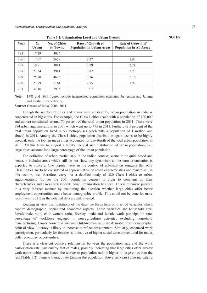
NOTES


Table 3.1: Urbanization Level and Urban Growth

Year %Urban

No. of Citiesor Towns

Rate of Growth ofPopulation in Urban Areas

Rate of Growth ofPopulation in All Areas

1951 17.29 3035

1961 17.97 2657 2.37 1.97

1971 19.91 3081 3.29 2.24

1981 23.34 3981 3.87 2.23

1991 25.70 4615 3.16 2.16

2001 27.79 5161 2.75 1.97

2011 31.16 7935 2.7

Note: 1981 and 1991 figures include interpolated population estimates for Assam and Jammuand Kashmir respectively.

Source: Census of India, 2001, 2011.

Though the number of cities and towns went up steadily, urban population in India isconcentrated in big cities. For example, the Class I cities (each with a population of 100,000and above) constituted around 70 percent of the total urban population in 2011. There were384 urban agglomerations in 2001 which went up to 475 in 2011. Further, 42.5 percent of thetotal urban population lived in 53 metropolises (each with a population of 1 million andabove) in 2011. Among the Class I cities, population distribution again seems to be highlyunequal: only the top ten mega cities accounted for one-fourth of the total urban population in2011. All this tends to suggest a highly unequal size distribution of urban population, i.e.,large cities account for a large percentage of the urban population.

The definition of urban, particularly in the Indian context, seems to be quite broad andhence, it includes areas which still do not show any dynamism as the term urbanization isexpected to indicate. One popular view in the context of urbanization suggests that onlyClass I cities are to be considered as representative of urban characteristics and dynamism. Inthis section, we, therefore, carry out a detailed study of 380 Class I cities or urbanagglomerations (as per the 2001 population census) in order to comment on theircharacteristics and assess how vibrant Indian urbanization has been. This is of course pursuedin a very indirect manner by examining the question whether large cities offer betteremployment opportunities and a better demographic profile. This could not be done for morerecent year (2011) as the detailed data are still awaited.

Keeping in view the limitations of the data, we focus here on a set of variables whichcapture demographic, social and economic aspects. These variables are household size,female-male ratio, child-woman ratio, literacy, male and female work participation rate,percentage of workforce engaged in non-agriculture activities excluding householdmanufacturing. Lower household size and child-woman ratio are desirable from demographicpoint of view. Literacy is likely to increase to reflect development. Similarly, enhanced workparticipation, particularly for females is indicative of higher social development and for males,better economic opportunities.

There is a clear-cut positive relationship between the population size and the workparticipation rate, particularly that of males, possibly indicating that large cities offer greaterwork opportunities and hence, the worker to population ratio is higher in large cities than therest (Table 3.2). Female literacy rate (among the population above six years) also indicates a

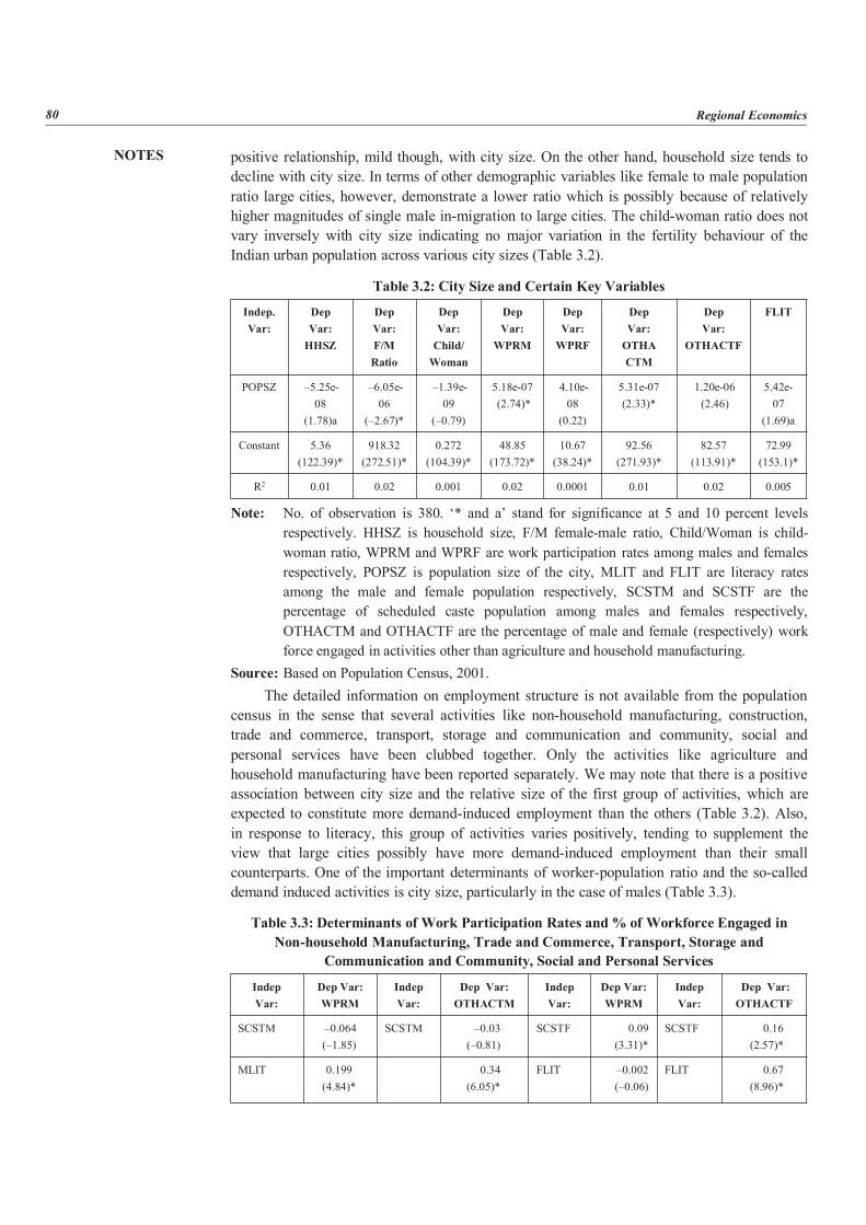
NOTES


positive relationship, mild though, with city size. On the other hand, household size tends todecline with city size. In terms of other demographic variables like female to male populationratio large cities, however, demonstrate a lower ratio which is possibly because of relativelyhigher magnitudes of single male in-migration to large cities. The child-woman ratio does notvary inversely with city size indicating no major variation in the fertility behaviour of theIndian urban population across various city sizes (Table 3.2).

Table 3.2: City Size and Certain Key Variables

Indep.Var:

DepVar:HHSZ

DepVar:F/MRatio

DepVar:Child/Woman

DepVar:WPRM

DepVar:WPRF

DepVar:OTHACTM

DepVar:

OTHACTF

FLIT

POPSZ –5.25e-08

(1.78)a

–6.05e-06

(–2.67)*

–1.39e-09

(–0.79)

5.18e-07(2.74)*

4.10e-08(0.22)

5.31e-07(2.33)*

1.20e-06(2.46)

5.42e-07

(1.69)a

Constant 5.36(122.39)*

918.32(272.51)*

0.272(104.39)*

48.85(173.72)*

10.67(38.24)*

92.56(271.93)*

82.57(113.91)*

72.99(153.1)*

R2 0.01 0.02 0.001 0.02 0.0001 0.01 0.02 0.005

Note: No. of observation is 380. ‘* and a’ stand for significance at 5 and 10 percent levelsrespectively. HHSZ is household size, F/M female-male ratio, Child/Woman is child-woman ratio, WPRM and WPRF are work participation rates among males and femalesrespectively, POPSZ is population size of the city, MLIT and FLIT are literacy ratesamong the male and female population respectively, SCSTM and SCSTF are thepercentage of scheduled caste population among males and females respectively,OTHACTM and OTHACTF are the percentage of male and female (respectively) workforce engaged in activities other than agriculture and household manufacturing.

Source: Based on Population Census, 2001.The detailed information on employment structure is not available from the population

census in the sense that several activities like non-household manufacturing, construction,trade and commerce, transport, storage and communication and community, social andpersonal services have been clubbed together. Only the activities like agriculture andhousehold manufacturing have been reported separately. We may note that there is a positiveassociation between city size and the relative size of the first group of activities, which areexpected to constitute more demand-induced employment than the others (Table 3.2). Also,in response to literacy, this group of activities varies positively, tending to supplement theview that large cities possibly have more demand-induced employment than their smallcounterparts. One of the important determinants of worker-population ratio and the so-calleddemand induced activities is city size, particularly in the case of males (Table 3.3).

Table 3.3: Determinants of Work Participation Rates and% of Workforce Engaged inNon-household Manufacturing, Trade and Commerce, Transport, Storage and

Communication and Community, Social and Personal Services

IndepVar:

Dep Var:WPRM

IndepVar:

Dep Var:OTHACTM

IndepVar:

Dep Var:WPRM

IndepVar:

Dep Var:OTHACTF

SCSTM –0.064(–1.85)

SCSTM –0.03(–0.81)

SCSTF 0.09(3.31)*

SCSTF 0.16(2.57)*

MLIT 0.199(4.84)*

0.34(6.05)*

FLIT –0.002(–0.06)

FLIT 0.67(8.96)*

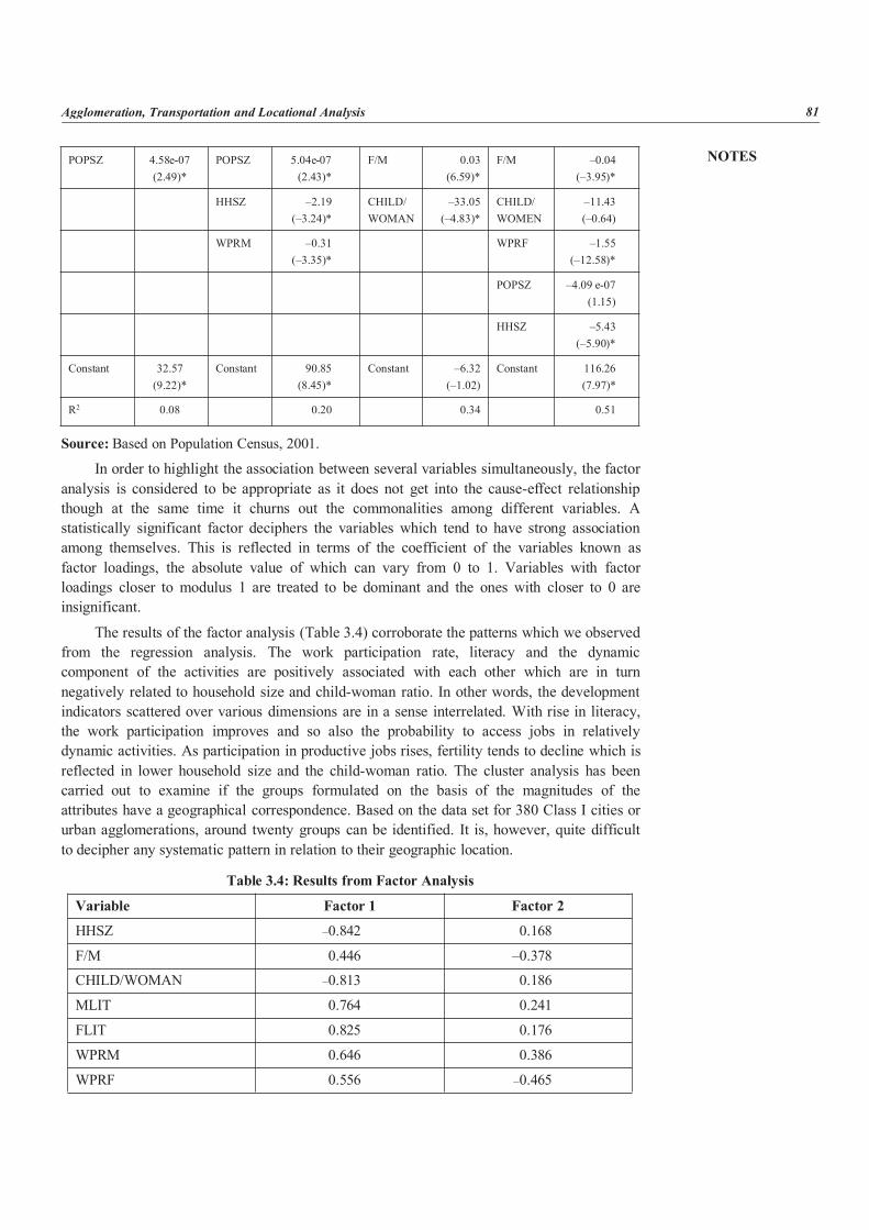
NOTES


POPSZ 4.58e-07(2.49)*

POPSZ 5.04e-07(2.43)*

F/M 0.03(6.59)*

F/M –0.04(–3.95)*

HHSZ –2.19(–3.24)*

CHILD/WOMAN

–33.05(–4.83)*

CHILD/WOMEN

–11.43(–0.64)

WPRM –0.31(–3.35)*

WPRF –1.55(–12.58)*

POPSZ –4.09 e-07(1.15)

HHSZ –5.43(–5.90)*

Constant 32.57(9.22)*

Constant 90.85(8.45)*

Constant –6.32(–1.02)

Constant 116.26(7.97)*

R2 0.08 0.20 0.34 0.51

Source: Based on Population Census, 2001.

In order to highlight the association between several variables simultaneously, the factoranalysis is considered to be appropriate as it does not get into the cause-effect relationshipthough at the same time it churns out the commonalities among different variables. Astatistically significant factor deciphers the variables which tend to have strong associationamong themselves. This is reflected in terms of the coefficient of the variables known asfactor loadings, the absolute value of which can vary from 0 to 1. Variables with factorloadings closer to modulus 1 are treated to be dominant and the ones with closer to 0 areinsignificant.

The results of the factor analysis (Table 3.4) corroborate the patterns which we observedfrom the regression analysis. The work participation rate, literacy and the dynamiccomponent of the activities are positively associated with each other which are in turnnegatively related to household size and child-woman ratio. In other words, the developmentindicators scattered over various dimensions are in a sense interrelated. With rise in literacy,the work participation improves and so also the probability to access jobs in relativelydynamic activities. As participation in productive jobs rises, fertility tends to decline which isreflected in lower household size and the child-woman ratio. The cluster analysis has beencarried out to examine if the groups formulated on the basis of the magnitudes of theattributes have a geographical correspondence. Based on the data set for 380 Class I cities orurban agglomerations, around twenty groups can be identified. It is, however, quite difficultto decipher any systematic pattern in relation to their geographic location.

Table 3.4: Results from Factor Analysis

Variable Factor 1 Factor 2

HHSZ –0.842 0.168

F/M 0.446 –0.378

CHILD/WOMAN –0.813 0.186

MLIT 0.764 0.241

FLIT 0.825 0.176

WPRM 0.646 0.386

WPRF 0.556 –0.465

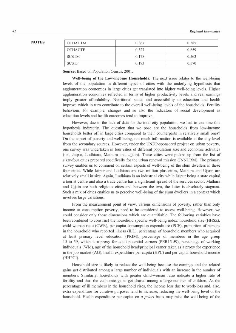
NOTES


OTHACTM 0.367 0.585

OTHACTF 0.327 0.659

SCSTM 0.178 0.563

SCSTF 0.193 0.570

Source: Based on Population Census, 2001.

Well-being of the Low-income Households: The next issue relates to the well-beinglevels of the population in different types of cities with the underlying hypothesis thatagglomeration economies in large cities get translated into higher well-being levels. Higheragglomeration economies reflected in terms of higher productivity levels and real earningsimply greater affordability. Nutritional status and accessibility to education and healthimprove which in turn contribute to the overall well-being levels of the households. Fertilitybehaviour, for example, changes and so also the indicators of social development aseducation levels and health outcomes tend to improve.

However, due to the lack of data for the total city population, we had to examine thishypothesis indirectly. The question that we pose are the households from low-incomehouseholds better off in large cities compared to their counterparts in relatively small ones?On the aspect of poverty and well-being, not much information is available at the city levelfrom the secondary sources. However, under the UNDP-sponsored project on urban poverty,one survey was undertaken in four cities of different population size and economic activities(i.e., Jaipur, Ludhiana, Mathura and Ujjain). These cities were picked up from the list ofsixty-four cities prepared specifically for the urban renewal mission (JNNURM). The primarysurvey enables us to comment on certain aspects of well-being of the slum dwellers in thesefour cities. While Jaipur and Ludhiana are two million plus cities, Mathura and Ujjain arerelatively small in size. Again, Ludhiana is an industrial city while Jaipur being a state capital,a tourist centre and also a trade centre has a significant spread of the services sector. Mathuraand Ujjain are both religious cities and between the two, the latter is absolutely stagnant.Such a mix of cities enables us to perceive well-being of the slum dwellers in a context whichinvolves large variations.

From the measurement point of view, various dimensions of poverty, rather than onlyincome or consumption poverty, need to be considered to assess well-being. However, wecould consider only those dimensions which are quantifiable. The following variables havebeen combined to construct the household specific well-being index: household size (HHSZ),child-woman ratio (CWR), per capita consumption expenditure (PCE), proportion of personsin the household who reported illness (ILL), percentage of household members who acquiredat least primary level education (PRIM), percentage of members in the age group15 to 59, which is a proxy for adult potential earners (PER15-59), percentage of workingindividuals (WM), age of the household head/principal earner taken as a proxy for experiencein the job market (AG), health expenditure per capita (HPC) and per capita household income(HHPCI).

Household size is likely to reduce the well-being because the earnings and the relatedgains get distributed among a large number of individuals with an increase in the number ofmembers. Similarly, households with greater child-woman ratio indicate a higher rate offertility and thus the economic gains get shared among a large number of children. As thepercentage of ill members in the household rises, the income loss due to work-loss and, also,extra expenditure for curative purposes tend to increase, reducing the well-being level of thehousehold. Health expenditure per capita on a priori basis may raise the well-being of the

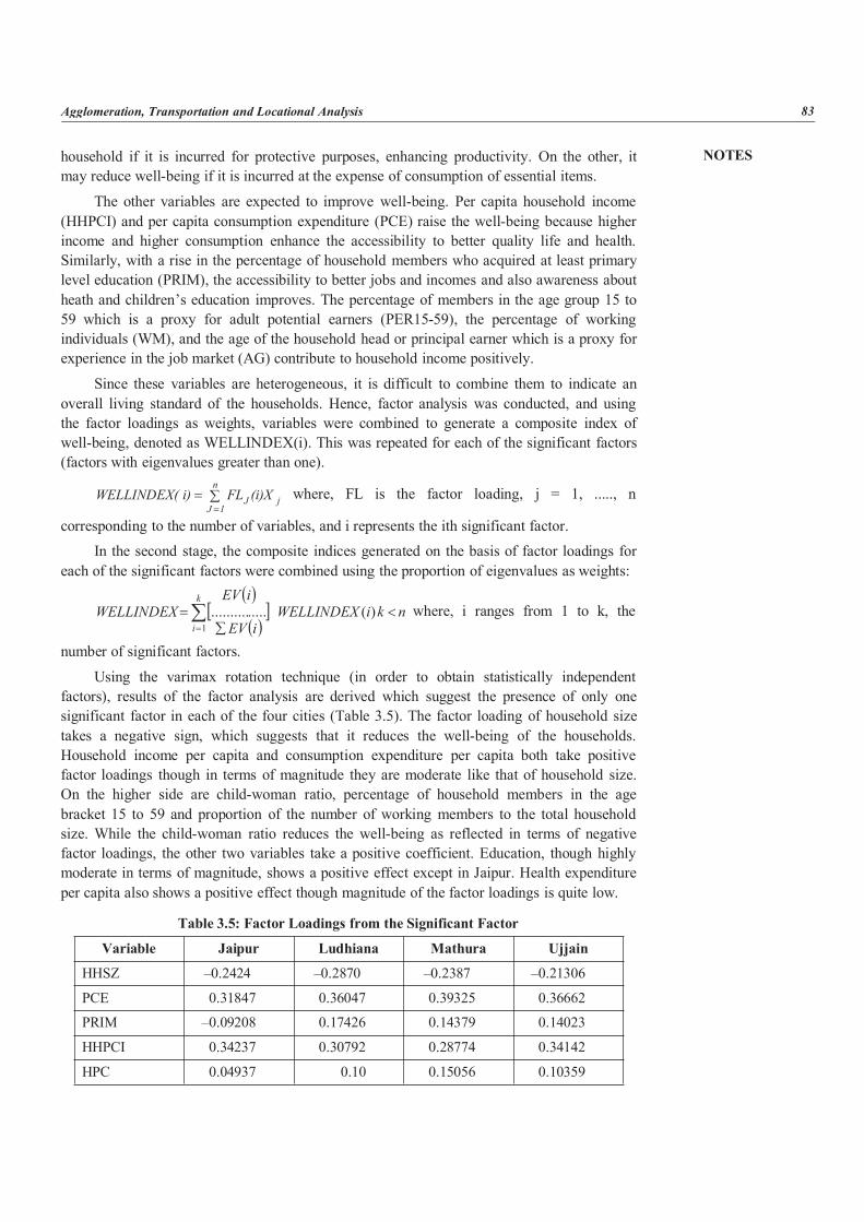
NOTES


household if it is incurred for protective purposes, enhancing productivity. On the other, itmay reduce well-being if it is incurred at the expense of consumption of essential items.

The other variables are expected to improve well-being. Per capita household income(HHPCI) and per capita consumption expenditure (PCE) raise the well-being because higherincome and higher consumption enhance the accessibility to better quality life and health.Similarly, with a rise in the percentage of household members who acquired at least primarylevel education (PRIM), the accessibility to better jobs and incomes and also awareness aboutheath and children’s education improves. The percentage of members in the age group 15 to59 which is a proxy for adult potential earners (PER15-59), the percentage of workingindividuals (WM), and the age of the household head or principal earner which is a proxy forexperience in the job market (AG) contribute to household income positively.

Since these variables are heterogeneous, it is difficult to combine them to indicate anoverall living standard of the households. Hence, factor analysis was conducted, and usingthe factor loadings as weights, variables were combined to generate a composite index ofwell-being, denoted as WELLINDEX(i). This was repeated for each of the significant factors(factors with eigenvalues greater than one).

n

1JjJ (i)XFLi)WELLINDEX( where, FL is the factor loading, j = 1, ....., n

corresponding to the number of variables, and i represents the ith significant factor.In the second stage, the composite indices generated on the basis of factor loadings for

each of the significant factors were combined using the proportion of eigenvalues as weights:

nkiWELLINDEXiEV

iEVWELLINDEX

k

i

)(...............

1where, i ranges from 1 to k, the

number of significant factors.

Using the varimax rotation technique (in order to obtain statistically independentfactors), results of the factor analysis are derived which suggest the presence of only onesignificant factor in each of the four cities (Table 3.5). The factor loading of household sizetakes a negative sign, which suggests that it reduces the well-being of the households.Household income per capita and consumption expenditure per capita both take positivefactor loadings though in terms of magnitude they are moderate like that of household size.On the higher side are child-woman ratio, percentage of household members in the agebracket 15 to 59 and proportion of the number of working members to the total householdsize. While the child-woman ratio reduces the well-being as reflected in terms of negativefactor loadings, the other two variables take a positive coefficient. Education, though highlymoderate in terms of magnitude, shows a positive effect except in Jaipur. Health expenditureper capita also shows a positive effect though magnitude of the factor loadings is quite low.

Table 3.5: Factor Loadings from the Significant Factor

Variable Jaipur Ludhiana Mathura Ujjain

HHSZ –0.2424 –0.2870 –0.2387 –0.21306

PCE 0.31847 0.36047 0.39325 0.36662

PRIM –0.09208 0.17426 0.14379 0.14023

HHPCI 0.34237 0.30792 0.28774 0.34142

HPC 0.04937 0.10 0.15056 0.10359

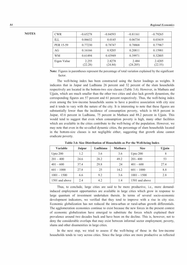
NOTES


CWR –0.65278 –0.84593 –0.81161 –0.79265

ILL 0.06632 0.0145 0.06734 0.03419

PER 15-59 0.77230 0.78747 0.78868 0.77967

AG 0.16166 0.9205 0.20811 0.15901

WM 0.61494 0.43949 0.39971 0.32805

Eigen Value 2.255(22.28)

2.8278(24.84)

2.484(24.205)

2.4205(22.55)

Note: Figures in parentheses represent the percentage of total variation explained by the significantfactor.

The well-being index has been constructed using the factor loadings as weights. Itindicates that in Jaipur and Ludhiana 26 percent and 32 percent of the slum householdsrespectively are located in the bottom-two size classes (Table 3.6). However, in Mathura andUjjain, which are much smaller than the other two cities and also lack growth dynamism, thecorresponding figures are 57 percent and 61 percent respectively. Thus, the well-being indexeven among the low-income households seems to have a positive association with city sizeand it tends to vary with the nature of the city. It is interesting to note that these figures aresubstantially lower than the incidence of consumption poverty, which is 66.8 percent inJaipur, 43.6 percent in Ludhiana, 75 percent in Mathura and 88.2 percent in Ujjain. Thiswould tend to suggest that even when consumption poverty is high, many other facilitieswhich are available in the cities contribute to the well-being of the population. However, wemay note that even in the so-called dynamic cities, the percentage of slum households locatedin the bottom-size classes is not negligible either, suggesting that growth alone cannoteradicate poverty.

Table 3.6: Size Distribution of Households as Per the Well-being Index

Variable Jaipur Ludhiana Mathura Size Ujjain

Upto 200 1.2 3.6 3.6 Upto 200 8

201 – 400 24.6 28.2 49.2 201- 400 53

401 – 600 37.4 29.8 24 401 – 600 27.4

601 – 1000 27.8 25 14.2 601 – 1000 8.8

1001 – 1500 6.6 9.2 3.6 1001 – 1500 2.8

1501 and above 2.4 4.2 1.4 1501 and above

Thus, to conclude, large cities are said to be more productive, i.e., more demand-induced employment opportunities are available in large cities which grow in response tolarge quantum of investment undertaken therein. In terms of several socio-economicdevelopment indicators, we verified that they tend to improve with a rise in city size.Economic globalization has not reduced the intra-urban or rural-urban growth differentials.The agglomeration economies continue to exist because the new forces in the present contextof economic globalization have emerged to substitute the forces which explained theirprevalence around two decades back and have been on the decline. This is, however, not todeny the considerable overlaps that may exist between informal sector employment, poverty,slums and other disamenities in large cities.

In the next step, we tried to assess if the well-being of those in the low-incomehouseholds tends to vary across cities. Since the large cities are more productive as reflected

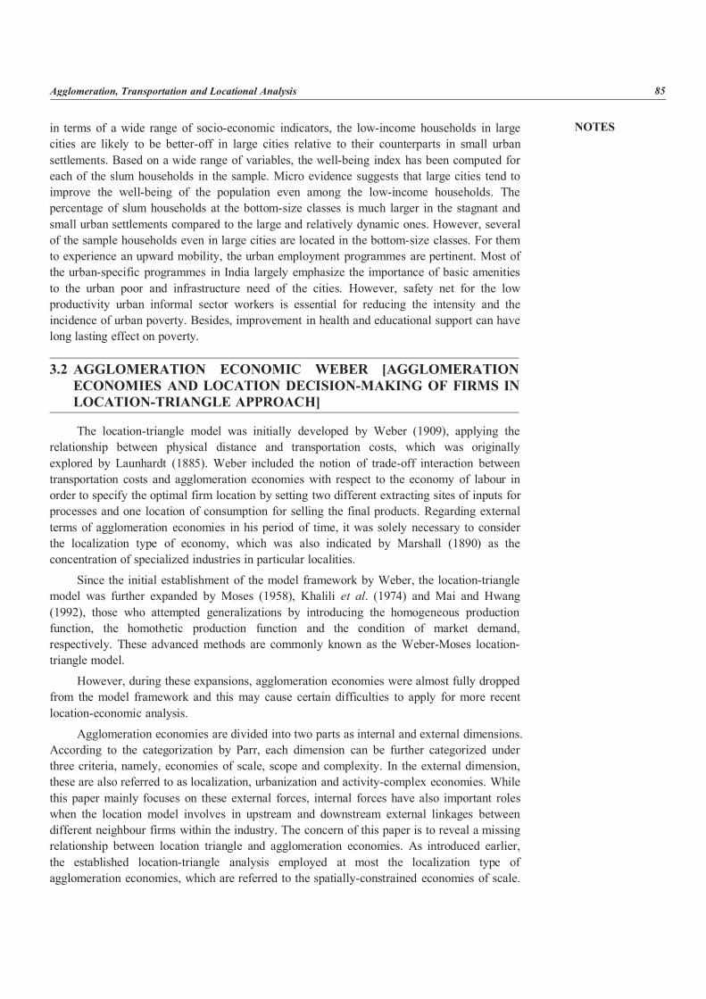
NOTES


in terms of a wide range of socio-economic indicators, the low-income households in largecities are likely to be better-off in large cities relative to their counterparts in small urbansettlements. Based on a wide range of variables, the well-being index has been computed foreach of the slum households in the sample. Micro evidence suggests that large cities tend toimprove the well-being of the population even among the low-income households. Thepercentage of slum households at the bottom-size classes is much larger in the stagnant andsmall urban settlements compared to the large and relatively dynamic ones. However, severalof the sample households even in large cities are located in the bottom-size classes. For themto experience an upward mobility, the urban employment programmes are pertinent. Most ofthe urban-specific programmes in India largely emphasize the importance of basic amenitiesto the urban poor and infrastructure need of the cities. However, safety net for the lowproductivity urban informal sector workers is essential for reducing the intensity and theincidence of urban poverty. Besides, improvement in health and educational support can havelong lasting effect on poverty.

3.2 AGGLOMERATION ECONOMIC WEBER [AGGLOMERATIONECONOMIES AND LOCATION DECISION-MAKING OF FIRMS INLOCATION-TRIANGLE APPROACH]

The location-triangle model was initially developed by Weber (1909), applying therelationship between physical distance and transportation costs, which was originallyexplored by Launhardt (1885). Weber included the notion of trade-off interaction betweentransportation costs and agglomeration economies with respect to the economy of labour inorder to specify the optimal firm location by setting two different extracting sites of inputs forprocesses and one location of consumption for selling the final products. Regarding externalterms of agglomeration economies in his period of time, it was solely necessary to considerthe localization type of economy, which was also indicated by Marshall (1890) as theconcentration of specialized industries in particular localities.

Since the initial establishment of the model framework by Weber, the location-trianglemodel was further expanded by Moses (1958), Khalili et al. (1974) and Mai and Hwang(1992), those who attempted generalizations by introducing the homogeneous productionfunction, the homothetic production function and the condition of market demand,respectively. These advanced methods are commonly known as the Weber-Moses location-triangle model.

However, during these expansions, agglomeration economies were almost fully droppedfrom the model framework and this may cause certain difficulties to apply for more recentlocation-economic analysis.

Agglomeration economies are divided into two parts as internal and external dimensions.According to the categorization by Parr, each dimension can be further categorized underthree criteria, namely, economies of scale, scope and complexity. In the external dimension,these are also referred to as localization, urbanization and activity-complex economies. Whilethis paper mainly focuses on these external forces, internal forces have also important roleswhen the location model involves in upstream and downstream external linkages betweendifferent neighbour firms within the industry. The concern of this paper is to reveal a missingrelationship between location triangle and agglomeration economies. As introduced earlier,the established location-triangle analysis employed at most the localization type ofagglomeration economies, which are referred to the spatially-constrained economies of scale.

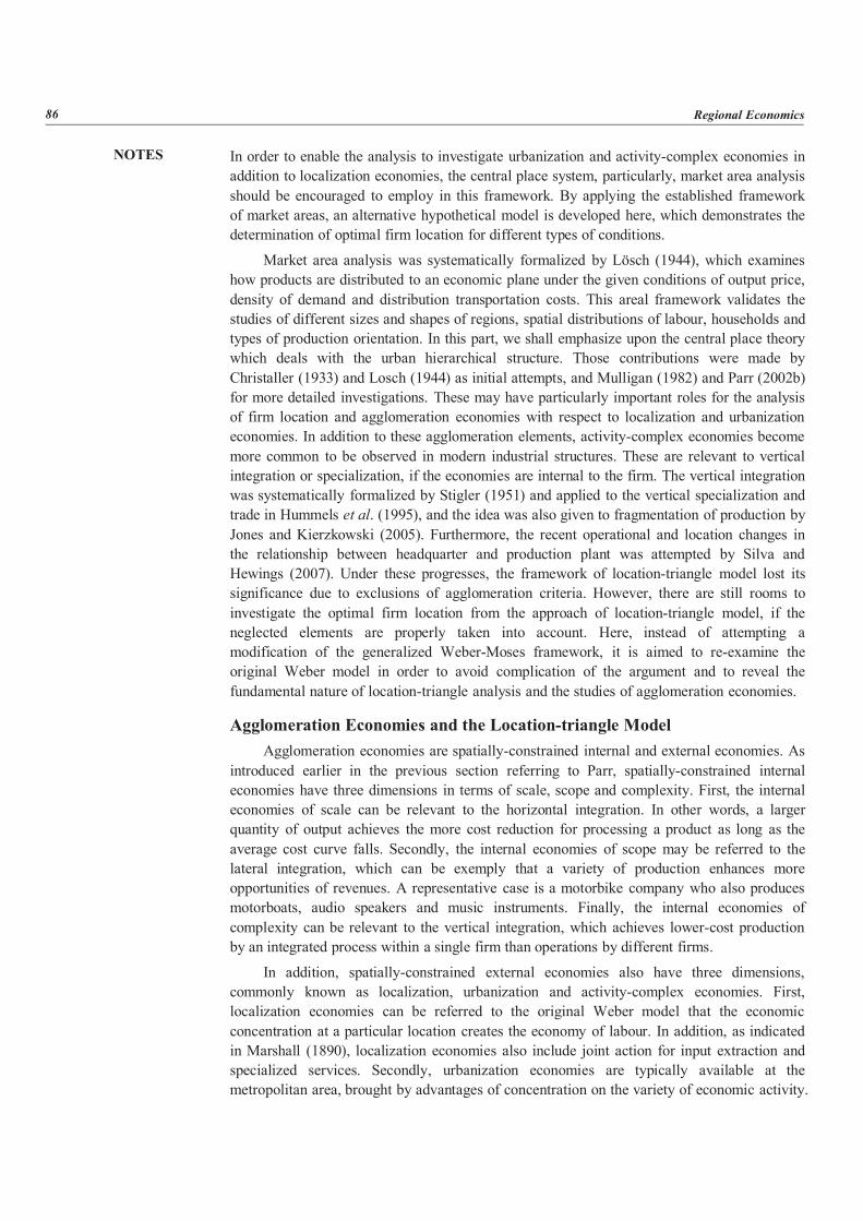
NOTES


In order to enable the analysis to investigate urbanization and activity-complex economies inaddition to localization economies, the central place system, particularly, market area analysisshould be encouraged to employ in this framework. By applying the established frameworkof market areas, an alternative hypothetical model is developed here, which demonstrates thedetermination of optimal firm location for different types of conditions.

Market area analysis was systematically formalized by Lösch (1944), which examineshow products are distributed to an economic plane under the given conditions of output price,density of demand and distribution transportation costs. This areal framework validates thestudies of different sizes and shapes of regions, spatial distributions of labour, households andtypes of production orientation. In this part, we shall emphasize upon the central place theorywhich deals with the urban hierarchical structure. Those contributions were made byChristaller (1933) and Losch (1944) as initial attempts, and Mulligan (1982) and Parr (2002b)for more detailed investigations. These may have particularly important roles for the analysisof firm location and agglomeration economies with respect to localization and urbanizationeconomies. In addition to these agglomeration elements, activity-complex economies becomemore common to be observed in modern industrial structures. These are relevant to verticalintegration or specialization, if the economies are internal to the firm. The vertical integrationwas systematically formalized by Stigler (1951) and applied to the vertical specialization andtrade in Hummels et al. (1995), and the idea was also given to fragmentation of production byJones and Kierzkowski (2005). Furthermore, the recent operational and location changes inthe relationship between headquarter and production plant was attempted by Silva andHewings (2007). Under these progresses, the framework of location-triangle model lost itssignificance due to exclusions of agglomeration criteria. However, there are still rooms toinvestigate the optimal firm location from the approach of location-triangle model, if theneglected elements are properly taken into account. Here, instead of attempting amodification of the generalized Weber-Moses framework, it is aimed to re-examine theoriginal Weber model in order to avoid complication of the argument and to reveal thefundamental nature of location-triangle analysis and the studies of agglomeration economies.

Agglomeration Economies and the Location-triangle ModelAgglomeration economies are spatially-constrained internal and external economies. As

introduced earlier in the previous section referring to Parr, spatially-constrained internaleconomies have three dimensions in terms of scale, scope and complexity. First, the internaleconomies of scale can be relevant to the horizontal integration. In other words, a largerquantity of output achieves the more cost reduction for processing a product as long as theaverage cost curve falls. Secondly, the internal economies of scope may be referred to thelateral integration, which can be exemply that a variety of production enhances moreopportunities of revenues. A representative case is a motorbike company who also producesmotorboats, audio speakers and music instruments. Finally, the internal economies ofcomplexity can be relevant to the vertical integration, which achieves lower-cost productionby an integrated process within a single firm than operations by different firms.

In addition, spatially-constrained external economies also have three dimensions,commonly known as localization, urbanization and activity-complex economies. First,localization economies can be referred to the original Weber model that the economicconcentration at a particular location creates the economy of labour. In addition, as indicatedin Marshall (1890), localization economies also include joint action for input extraction andspecialized services. Secondly, urbanization economies are typically available at themetropolitan area, brought by advantages of concentration on the variety of economic activity.

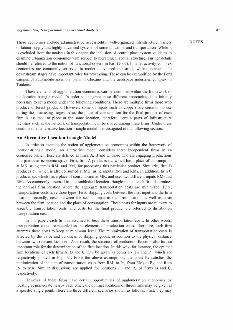
NOTES


These economies include administrative accessibility, well-organized infrastructure, varietyof labour supply and highly-advanced systems of communication and transportation. While itis excluded from the analysis in this paper, the inclusion of central place system validates toexamine urbanization economies with respect to hierarchical spatial structure. Further detailsshould be referred to the notion of functional system in Parr (2007). Finally, activity-complexeconomies are commonly observed in modern advanced industries, where upstream anddownstream stages have important roles for processing. These can be exemplified by the Fordcampus of automobile-assembly plant in Chicago and the aerospace industries complex inToulouse.

Those elements of agglomeration economies can be examined within the framework ofthe location-triangle model. In order to integrate these different approaches, it is initiallynecessary to set a model under the following conditions. There are multiple firms those whoproduce different products. However, some of inputs such as coppers are common to useduring the processing stages. Also, the place of consumption for the final product of eachfirm is assumed to place at the same location, therefore, certain parts of infrastructurefacilities such as the network of transportation can be shared among these firms. Under theseconditions, an alternative location-triangle model is investigated in the following section.

An Alternative Location-triangle ModelIn order to examine the notion of agglomeration economies within the framework of

location-triangle model, an alternative model considers three independent firms in aneconomic plane. These are defined as firms A, B and C, those who are engaging productionsin a particular economic space. First, firm A produces qA, which has a place of consumptionat MK, using inputs RM1 and RM2 for processing this particular product. Similarly, firm Bproduces qB, which is also consumed at MK, using inputs RM2 and RM3. In addition, firm Cproduces qC, which has a place of consumption at MK, and uses two different inputs RM2 andRM4. As commonly assumed in the established location-triangle model, each firm determinesthe optimal firm location where the aggregate transportation costs are minimized. Here,transportation costs have three types. First, shipping costs between the first input and the firmlocation, secondly, costs between the second input to the firm location as well as costsbetween the firm location and the place of consumption. These costs for inputs are relevant toassembly transportation costs, and costs for the final product are referred to distributiontransportation costs.

In this paper, each firm is assumed to bear these transportation costs. In other words,transportation costs are regarded as the elements of production costs. Therefore, each firmattempts these costs to keep at minimum level. The minimization of transportation costs isaffected by the value and bulkiness of shipping goods, in addition to the physical distancebetween two relevant locations. As a result, the structure of production function also has animportant role for the determination of the firm location. In this way, for instance, the optimalfirm locations of each firm A, B and C may be given as points PA, PB and PC, which arerespectively plotted in Fig. 3.1. From the above assumptions, the point PA satisfies theminimization of the sum of transportation costs from RM1 to PA, from RM2 to PA, and fromPA to MK. Similar discussions are applied for locations PB and PC of firms B and C,respectively.

However, if these firms have certain opportunities of agglomeration economies bylocating at immediate nearby each other, the optimal locations of three firms may be given ata specific single point. There are three different scenarios shown as follows. First, they may

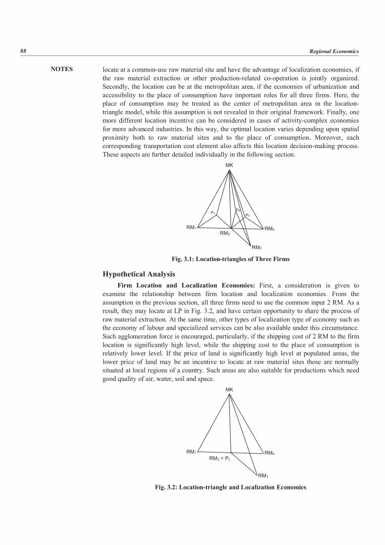
NOTES


locate at a common-use raw material site and have the advantage of localization economies, ifthe raw material extraction or other production-related co-operation is jointly organized.Secondly, the location can be at the metropolitan area, if the economies of urbanization andaccessibility to the place of consumption have important roles for all three firms. Here, theplace of consumption may be treated as the center of metropolitan area in the location-triangle model, while this assumption is not revealed in their original framework. Finally, onemore different location incentive can be considered in cases of activity-complex economiesfor more advanced industries. In this way, the optimal location varies depending upon spatialproximity both to raw material sites and to the place of consumption. Moreover, eachcorresponding transportation cost element also affects this location decision-making process.These aspects are further detailed individually in the following section.

MK

RM1RM2

RM4

RM3

PAPB

PC

Fig. 3.1: Location-triangles of Three Firms

Hypothetical AnalysisFirm Location and Localization Economies: First, a consideration is given to

examine the relationship between firm location and localization economies. From theassumption in the previous section, all three firms need to use the common input 2 RM. As aresult, they may locate at LP in Fig. 3.2, and have certain opportunity to share the process ofraw material extraction. At the same time, other types of localization type of economy such asthe economy of labour and specialized services can be also available under this circumstance.Such agglomeration force is encouraged, particularly, if the shipping cost of 2 RM to the firmlocation is significantly high level, while the shipping cost to the place of consumption isrelatively lower level. If the price of land is significantly high level at populated areas, thelower price of land may be an incentive to locate at raw material sites those are normallysituated at local regions of a country. Such areas are also suitable for productions which needgood quality of air, water, soil and space.

RM1

MK

RM2 = PLRM4

RM3

Fig. 3.2: Location-triangle and Localization Economies

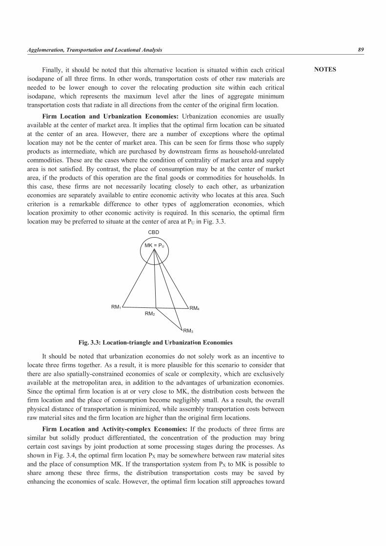
NOTES


Finally, it should be noted that this alternative location is situated within each criticalisodapane of all three firms. In other words, transportation costs of other raw materials areneeded to be lower enough to cover the relocating production site within each criticalisodapane, which represents the maximum level after the lines of aggregate minimumtransportation costs that radiate in all directions from the center of the original firm location.

Firm Location and Urbanization Economies: Urbanization economies are usuallyavailable at the center of market area. It implies that the optimal firm location can be situatedat the center of an area. However, there are a number of exceptions where the optimallocation may not be the center of market area. This can be seen for firms those who supplyproducts as intermediate, which are purchased by downstream firms as household-unrelatedcommodities. These are the cases where the condition of centrality of market area and supplyarea is not satisfied. By contrast, the place of consumption may be at the center of marketarea, if the products of this operation are the final goods or commodities for households. Inthis case, these firms are not necessarily locating closely to each other, as urbanizationeconomies are separately available to entire economic activity who locates at this area. Suchcriterion is a remarkable difference to other types of agglomeration economies, whichlocation proximity to other economic activity is required. In this scenario, the optimal firmlocation may be preferred to situate at the center of area at PU in Fig. 3.3.

RM4

RM3

RM2

MK = PU

RM1

CBD

Fig. 3.3: Location-triangle and Urbanization Economies

It should be noted that urbanization economies do not solely work as an incentive tolocate three firms together. As a result, it is more plausible for this scenario to consider thatthere are also spatially-constrained economies of scale or complexity, which are exclusivelyavailable at the metropolitan area, in addition to the advantages of urbanization economies.Since the optimal firm location is at or very close to MK, the distribution costs between thefirm location and the place of consumption become negligibly small. As a result, the overallphysical distance of transportation is minimized, while assembly transportation costs betweenraw material sites and the firm location are higher than the original firm locations.

Firm Location and Activity-complex Economies: If the products of three firms aresimilar but solidly product differentiated, the concentration of the production may bringcertain cost savings by joint production at some processing stages during the processes. Asshown in Fig. 3.4, the optimal firm location PX may be somewhere between raw material sitesand the place of consumption MK. If the transportation system from PX to MK is possible toshare among these three firms, the distribution transportation costs may be saved byenhancing the economies of scale. However, the optimal firm location still approaches toward

NOTES


the center MK, if the joint cost-saving distribution is significantly high level. By contrast, ifthe assembly transportation contains bulky and high-cost structure, they are locating close toraw material sites.

Also, the presence of CBD also leads to a similar outcome. namely, the larger CBDlocates the firm away from the center in order to avoid highly price of land, congestion andpollution. It can be refereed to the centrifugal forces of urbanization economies or moresimply urbanization diseconomies. In this way, agglomeration economies and transportationcosts have important roles to solve the problem of optimal firm location.

RM4

RM3

RM2

MK

RM1

CBD

PX

Fig. 3.4: Location-triangle and Activity-complex Economies

Policy ImplicationsIn order to generalize the alternative framework, the following cost function of a

representative firm is given:

Min C = ((wi + ti.di) xi + (wj + tj.dj) xj + α.tk dk.qk). β .....(1)

where wi = price of input i, ti = transportation cost rate for i, di = distance from the inputsite i to the firm location, xi = the amount of input i, wj = price of input j, tj = transportationcost rate for j, dj = distance from the input site j to the firm location, xj = the amount of input j, (0 < < 1) = cost saving index by sharing the distribution transportation system, tk =distribution transportation rate, dk = distance from the firm location to the place ofconsumption, qk = the quantity of product, and (0 < < 1) = index of the economies ofagglomeration.

Here, and are zero, if each firm establishes their plant location separately. In thatcase, each firm can minimize the sum of distance di, dj and dk. By contrast, the sum ofdistance cannot be minimized when a firm locates together with other two firms in order toobtain opportunities of agglomeration economies and shared distribution costs. In that case, and are set non-zero and certain cost saving may be available. This is a trade-off interactionbetween agglomeration economies and physical distance in Weber sense. However, aremarkable difference is that this analysis also includes the cost-saving opportunity ofdistribution transportation costs. The evaluation can be provided as follows. First, each firmdoes not locate together, if the benefit of and are less than the cost increase by additionaldistance of di, dj and dk. Otherwise, each firm locates together and the optimal firm locationvaries depend on the conditions given in Table 3.1.

As an exception, it should be noted that these firms are not locating at the place ofconsumption, if the diseconomies of urbanization are set significantly high level. In that case,

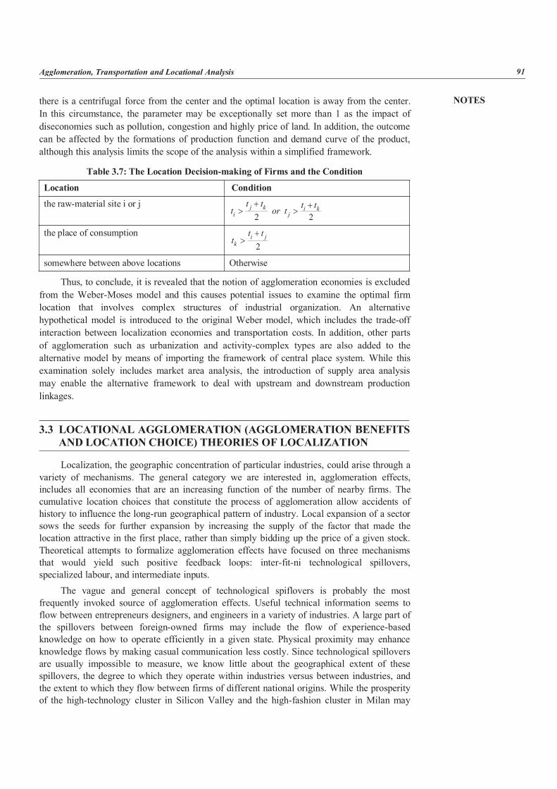
NOTES


there is a centrifugal force from the center and the optimal location is away from the center.In this circumstance, the parameter may be exceptionally set more than 1 as the impact ofdiseconomies such as pollution, congestion and highly price of land. In addition, the outcomecan be affected by the formations of production function and demand curve of the product,although this analysis limits the scope of the analysis within a simplified framework.

Table 3.7: The Location Decision-making of Firms and the Condition

Location Condition

the raw-material site i or j22

kij

kji

ttt or tt

t

the place of consumption2

jik

ttt

somewhere between above locations Otherwise

Thus, to conclude, it is revealed that the notion of agglomeration economies is excludedfrom the Weber-Moses model and this causes potential issues to examine the optimal firmlocation that involves complex structures of industrial organization. An alternativehypothetical model is introduced to the original Weber model, which includes the trade-offinteraction between localization economies and transportation costs. In addition, other partsof agglomeration such as urbanization and activity-complex types are also added to thealternative model by means of importing the framework of central place system. While thisexamination solely includes market area analysis, the introduction of supply area analysismay enable the alternative framework to deal with upstream and downstream productionlinkages.

3.3 LOCATIONAL AGGLOMERATION (AGGLOMERATION BENEFITSAND LOCATION CHOICE) THEORIES OF LOCALIZATION

Localization, the geographic concentration of particular industries, could arise through avariety of mechanisms. The general category we are interested in, agglomeration effects,includes all economies that are an increasing function of the number of nearby firms. Thecumulative location choices that constitute the process of agglomeration allow accidents ofhistory to influence the long-run geographical pattern of industry. Local expansion of a sectorsows the seeds for further expansion by increasing the supply of the factor that made thelocation attractive in the first place, rather than simply bidding up the price of a given stock.Theoretical attempts to formalize agglomeration effects have focused on three mechanismsthat would yield such positive feedback loops: inter-fit-ni technological spillovers,specialized labour, and intermediate inputs.

The vague and general concept of technological spiflovers is probably the mostfrequently invoked source of agglomeration effects. Useful technical information seems toflow between entrepreneurs designers, and engineers in a variety of industries. A large part ofthe spillovers between foreign-owned firms may include the flow of experience-basedknowledge on how to operate efficiently in a given state. Physical proximity may enhanceknowledge flows by making casual communication less costly. Since technological spilloversare usually impossible to measure, we know little about the geographical extent of thesespillovers, the degree to which they operate within industries versus between industries, andthe extent to which they flow between firms of different national origins. While the prosperityof the high-technology cluster in Silicon Valley and the high-fashion cluster in Milan may

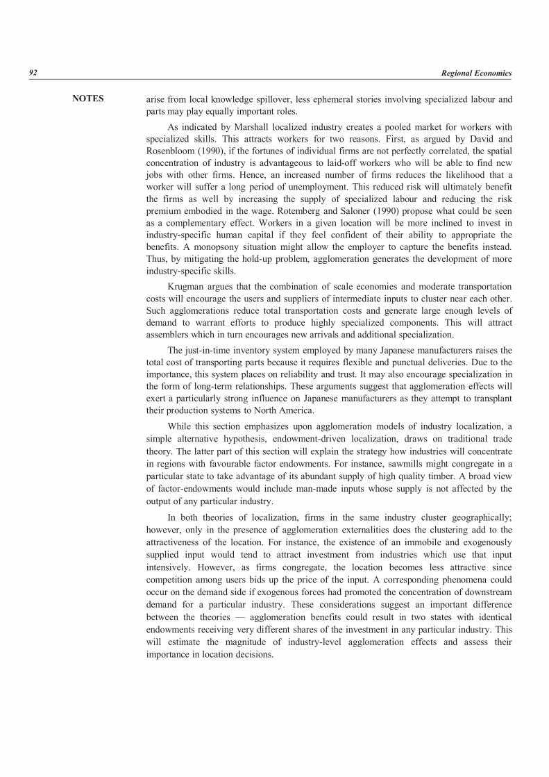
NOTES


arise from local knowledge spillover, less ephemeral stories involving specialized labour andparts may play equally important roles.

As indicated by Marshall localized industry creates a pooled market for workers withspecialized skills. This attracts workers for two reasons. First, as argued by David andRosenbloom (1990), if the fortunes of individual firms are not perfectly correlated, the spatialconcentration of industry is advantageous to laid-off workers who will be able to find newjobs with other firms. Hence, an increased number of firms reduces the likelihood that aworker will suffer a long period of unemployment. This reduced risk will ultimately benefitthe firms as well by increasing the supply of specialized labour and reducing the riskpremium embodied in the wage. Rotemberg and Saloner (1990) propose what could be seenas a complementary effect. Workers in a given location will be more inclined to invest inindustry-specific human capital if they feel confident of their ability to appropriate thebenefits. A monopsony situation might allow the employer to capture the benefits instead.Thus, by mitigating the hold-up problem, agglomeration generates the development of moreindustry-specific skills.

Krugman argues that the combination of scale economies and moderate transportationcosts will encourage the users and suppliers of intermediate inputs to cluster near each other.Such agglomerations reduce total transportation costs and generate large enough levels ofdemand to warrant efforts to produce highly specialized components. This will attractassemblers which in turn encourages new arrivals and additional specialization.

The just-in-time inventory system employed by many Japanese manufacturers raises thetotal cost of transporting parts because it requires flexible and punctual deliveries. Due to theimportance, this system places on reliability and trust. It may also encourage specialization inthe form of long-term relationships. These arguments suggest that agglomeration effects willexert a particularly strong influence on Japanese manufacturers as they attempt to transplanttheir production systems to North America.

While this section emphasizes upon agglomeration models of industry localization, asimple alternative hypothesis, endowment-driven localization, draws on traditional tradetheory. The latter part of this section will explain the strategy how industries will concentratein regions with favourable factor endowments. For instance, sawmills might congregate in aparticular state to take advantage of its abundant supply of high quality timber. A broad viewof factor-endowments would include man-made inputs whose supply is not affected by theoutput of any particular industry.

In both theories of localization, firms in the same industry cluster geographically;however, only in the presence of agglomeration externalities does the clustering add to theattractiveness of the location. For instance, the existence of an immobile and exogenouslysupplied input would tend to attract investment from industries which use that inputintensively. However, as firms congregate, the location becomes less attractive sincecompetition among users bids up the price of the input. A corresponding phenomena couldoccur on the demand side if exogenous forces had promoted the concentration of downstreamdemand for a particular industry. These considerations suggest an important differencebetween the theories — agglomeration benefits could result in two states with identicalendowments receiving very different shares of the investment in any particular industry. Thiswill estimate the magnitude of industry-level agglomeration effects and assess theirimportance in location decisions.

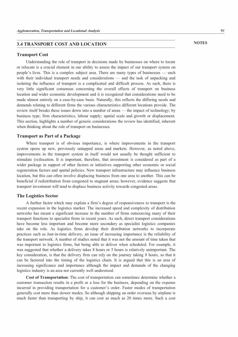
NOTES


3.4 TRANSPORT COST AND LOCATION

Transport CostUnderstanding the role of transport in decisions made by businesses on where to locate

or relocate is a crucial element in our ability to assess the impact of our transport system onpeople’s lives. This is a complex subject area. There are many types of businesses — eachwith their individual transport needs and considerations — and the task of unpacking andisolating the influence of transport is a complicated and difficult process. As such, there isvery little significant consensus concerning the overall effects of transport on businesslocation and wider economic development and it is recognized that considerations need to bemade almost entirely on a case-by-case basis. Naturally, this reflects the differing needs anddemands relating to different firms the various characteristics different locations provide. Thereview itself breaks these issues down into a number of areas — the impact of technology; bybusiness type; firm characteristics, labour supply; spatial scale and growth or displacement.This section, highlights a number of generic considerations the review has identified, inherentwhen thinking about the role of transport on businesses.

Transport as Part of a PackageWhere transport is of obvious importance, is where improvements in the transport

system opens up new, previously untapped areas and markets. However, as noted above,improvements in the transport system in itself would not usually be thought sufficient tostimulate (re)location. It is important, therefore, that investment is considered as part of awider package in support of other factors or initiatives supporting other economic or socialregeneration factors and spatial policies. New transport infrastructure may influence businesslocation, but this can often involve displacing business from one area to another. This can bebeneficial if redistribution from congested to stagnant areas; however, evidence suggests thattransport investment will tend to displace business activity towards congested areas.

The Logistics SectorA further factor which may explain a firm’s degree of responsiveness to transport is the

recent expansion in the logistics market. The increased speed and complexity of distributionnetworks has meant a significant increase in the number of firms outsourcing many of theirtransport functions to specialist firms in recent years. As such, direct transport considerationshave become less important and become more secondary as specialist logistics companiestake on the role. As logistics firms develop their distribution networks to incorporatepractices such as Just-in-time delivery, an issue of increasing importance is the reliability ofthe transport network. A number of studies noted that it was not the amount of time taken thatwas important to logistics firms, but being able to deliver when scheduled. For example, itwas suggested that whether a delivery takes 8 hours or 5 hours is relatively unimportant. Thekey consideration, is that the delivery firm can rely on the journey taking 8 hours, so that itcan be factored into the timing of the logistics chain. It is argued that this is an area ofincreasing significance and importance although the impact and demands of the changinglogistics industry is an area not currently well understood.

Cost of Transportation: The cost of transportation can sometimes determine whether acustomer transaction results in a profit or a loss for the business, depending on the expenseincurred in providing transportation for a customer’s order. Faster modes of transportationgenerally cost more than slower modes. So although shipping an order overseas by airplane ismuch faster than transporting by ship, it can cost as much as 20 times more. Such a cost

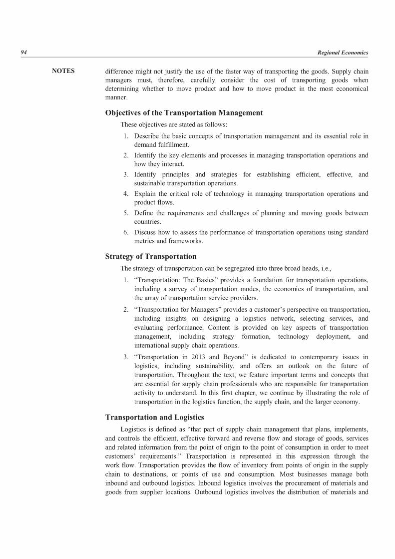
NOTES


difference might not justify the use of the faster way of transporting the goods. Supply chainmanagers must, therefore, carefully consider the cost of transporting goods whendetermining whether to move product and how to move product in the most economicalmanner.

Objectives of the Transportation ManagementThese objectives are stated as follows:1. Describe the basic concepts of transportation management and its essential role indemand fulfillment.

2. Identify the key elements and processes in managing transportation operations andhow they interact.

3. Identify principles and strategies for establishing efficient, effective, andsustainable transportation operations.

4. Explain the critical role of technology in managing transportation operations andproduct flows.

5. Define the requirements and challenges of planning and moving goods betweencountries.

6. Discuss how to assess the performance of transportation operations using standardmetrics and frameworks.

Strategy of TransportationThe strategy of transportation can be segregated into three broad heads, i.e.,

1. “Transportation: The Basics” provides a foundation for transportation operations,including a survey of transportation modes, the economics of transportation, andthe array of transportation service providers.

2. “Transportation for Managers” provides a customer’s perspective on transportation,including insights on designing a logistics network, selecting services, andevaluating performance. Content is provided on key aspects of transportationmanagement, including strategy formation, technology deployment, andinternational supply chain operations.

3. “Transportation in 2013 and Beyond” is dedicated to contemporary issues inlogistics, including sustainability, and offers an outlook on the future oftransportation. Throughout the text, we feature important terms and concepts thatare essential for supply chain professionals who are responsible for transportationactivity to understand. In this first chapter, we continue by illustrating the role oftransportation in the logistics function, the supply chain, and the larger economy.

Transportation and LogisticsLogistics is defined as “that part of supply chain management that plans, implements,

and controls the efficient, effective forward and reverse flow and storage of goods, servicesand related information from the point of origin to the point of consumption in order to meetcustomers’ requirements.” Transportation is represented in this expression through thework flow. Transportation provides the flow of inventory from points of origin in the supplychain to destinations, or points of use and consumption. Most businesses manage bothinbound and outbound logistics. Inbound logistics involves the procurement of materials andgoods from supplier locations. Outbound logistics involves the distribution of materials and

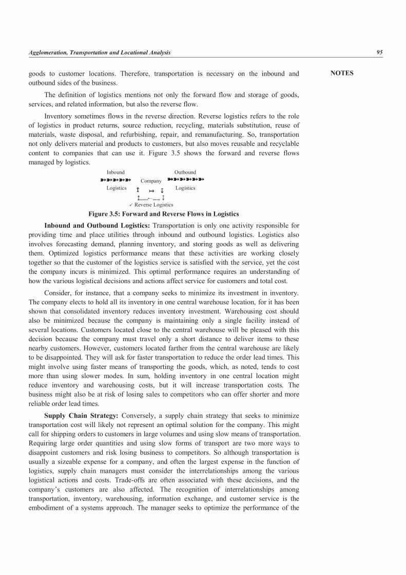
NOTES


goods to customer locations. Therefore, transportation is necessary on the inbound andoutbound sides of the business.

The definition of logistics mentions not only the forward flow and storage of goods,services, and related information, but also the reverse flow.

Inventory sometimes flows in the reverse direction. Reverse logistics refers to the roleof logistics in product returns, source reduction, recycling, materials substitution, reuse ofmaterials, waste disposal, and refurbishing, repair, and remanufacturing. So, transportationnot only delivers material and products to customers, but also moves reusable and recyclablecontent to companies that can use it. Figure 3.5 shows the forward and reverse flowsmanaged by logistics.

Inbound OutboundCompany

Logistics Logistics

↙ Reverse Logistics

Figure 3.5: Forward and Reverse Flows in Logistics

Inbound and Outbound Logistics: Transportation is only one activity responsible forproviding time and place utilities through inbound and outbound logistics. Logistics alsoinvolves forecasting demand, planning inventory, and storing goods as well as deliveringthem. Optimized logistics performance means that these activities are working closelytogether so that the customer of the logistics service is satisfied with the service, yet the costthe company incurs is minimized. This optimal performance requires an understanding ofhow the various logistical decisions and actions affect service for customers and total cost.

Consider, for instance, that a company seeks to minimize its investment in inventory.The company elects to hold all its inventory in one central warehouse location, for it has beenshown that consolidated inventory reduces inventory investment. Warehousing cost shouldalso be minimized because the company is maintaining only a single facility instead ofseveral locations. Customers located close to the central warehouse will be pleased with thisdecision because the company must travel only a short distance to deliver items to thesenearby customers. However, customers located farther from the central warehouse are likelyto be disappointed. They will ask for faster transportation to reduce the order lead times. Thismight involve using faster means of transporting the goods, which, as noted, tends to costmore than using slower modes. In sum, holding inventory in one central location mightreduce inventory and warehousing costs, but it will increase transportation costs. Thebusiness might also be at risk of losing sales to competitors who can offer shorter and morereliable order lead times.

Supply Chain Strategy: Conversely, a supply chain strategy that seeks to minimizetransportation cost will likely not represent an optimal solution for the company. This mightcall for shipping orders to customers in large volumes and using slow means of transportation.Requiring large order quantities and using slow forms of transport are two more ways todisappoint customers and risk losing business to competitors. So although transportation isusually a sizeable expense for a company, and often the largest expense in the function oflogistics, supply chain managers must consider the interrelationships among the variouslogistical actions and costs. Trade-offs are often associated with these decisions, and thecompany’s customers are also affected. The recognition of interrelationships amongtransportation, inventory, warehousing, information exchange, and customer service is theembodiment of a systems approach. The manager seeks to optimize the performance of the

NOTES


logistics system instead of optimizing a singular element of the system. This book, therefore,treats transportation as one important element of the logistics system.

Selection of the RegionSelecting a region for setting up an enterprise is dependent on the following factors:

Availability of Raw Materials: The availability of good quality raw materials inrequired quantity at close hand is very crucial for the success of a new enterprise. The regionmust have abundant supplies of atleast the chief raw material required by the firm. Such alocation helps to ensure continuity of production and reduces the transport costs. Few rawmaterials such as minerals, perishable food, cotton etc. play a vital role in influencing thelocation of the plant. For e.g., paper manufacturing plants require a regular supply of a largequantity of pure water and are, therefore, generally located near river banks.

Supply of Labour: The availability of the required grade of labour, i.e., skilled, semi-skilled or unskilled is an important factor influencing the location of the industry. Besides,the cost and productivity of labour, attitude of trade unions and the state of industrial relationsin a particular region are also important. This also explains concentration of certain industriesin certain states.

Proximity to the Product Market: An industry should ideally be located close to themarket for the product produced by the firm. This on one hand reduces the cost oftransporting the finished product to the market. On the other hand, it ensures maximization ofprofits by selling the goods at a competitive price. Generally, in case of the industries havingnational and international markets, plants are spread over wide geographical areas to haveclose proximity to all markets. In case of regional demand, plants are located near to theimmediate market.

Availability of Transport Facilities: A factory requires transport facilities both forgetting its raw materials as well as for reaching its finished products to the market. Hence,location is to be chosen in such a way that its total transport cost is the lowest. Of the twoelements of transport cost, which one will have a decisive influence on the decision oflocation will depend on the characteristics of the raw materials and the nature of themanufacturing process. If the factory requires bulky commodities like iron ore, limestone,etc., it should be situated nearer to the source of these raw material. But, if the manufacturingprocess is such that the raw materials loose a substantial part of its weight like in the case ofthe chemical and pharmaceutical products, the factory should be located nearer to the market.Therefore, a region which provides adequate transport facilities attracts industrialists.

Supply of Power: With increased mechanization, a location which ensures a regularand adequate supply of power and fuel for the business has become an indispensablerequirement.

Climatic Factors: Certain types of industries require a particular type of climate, e.g.,flour mills need a dry climate while cotton mills require a humid climate. Natural factors areparticularly important in extractive industries like plantations, fishing, agriculture, etc.Climate influences even the capacity to work on the part of the workers. But, thetechnological advancements like artificial humidification and air conditioning have reducedthe importance of climate as a factor.

Government Regulations and Policies: Central Government and the StateGovernments have made several policy announcements from time to time in order toencourage development of industries. Various incentive schemes have been provided to

NOTES


attract investment especially in backward areas. All this has become an important factorwhile selecting a suitable location.

Law and Order: Every entrepreneur is concerned about law and order as well as thepolitical stability of the area around which he wants to set up his industry. It is only naturalfor every entrepreneur to locate his unit in those areas which are not subject to riots andpolitical disturbances. No industrialist can ignore such national and strategic considerationswhile selecting the location of the industry.

Existence of Complementary and Competitive Industries: Such a location on onehand provides backward and forward linkages for the industries and on the other hand itprovides a competitive environment for them. It increases the supply of the required rawmaterials and enhances the demand for the goods produced. It improves the labour market byattracting both skilled and unskilled manpower. It also improves the banking, credit andcommunication facilities in the area. It brings into existence various commercial services likewarehousing, packing, forwarding, grading, appraising, advertising, etc. which helps in thegrowth and expansion of all the business firms in the particular area.

3.5 LOCATIONAL INTERDEPENDENCE

Changes in the Business EnvironmentThe environment within which different businesses operate is complex and ever

changing. Advances in ICT provision has altered this context in a number of significant wayswhich have an impact on the way the world and transport is viewed and utilized.Improvement in Communication Technology (ICT) has allowed us to develop new ways ofworking and communicating instantaneously with a large number of people, spread across arange of physical locations and distances and provided us with the potential flexibility towork wherever and whenever we want. This is a complex interrelationship with bettercommunication potentially reducing the need for travel, but on the other hand reinforcing orpossibly expanding travel demand as new markets and localities are opened. This is still arelatively nascent area of study and not surprisingly, there is little hard evidence — norconsensus — over the potential impacts that ICT has on travel demand.

A Necessary, But Not a Sufficient ConditionCompiled from business surveys, important factors commonly cited as important in

considering a location include:(i) the quality and scope of physical and business infrastructures;(ii) factor cost and supply, especially labour;(iii) market demand and links to international markets;(iv) institutional infrastructure and networks;(v) a culture supporting civicness and entrepreneurship;(vi) indigenous company growth;(vii) agglomeration economies;(viii) technological development;(ix) as well as more social factors such as climate, lifestyle, image and crime rates.Although some of these have an element of transport within these, none directly relate

to transport per se.

NOTES


As a general rule, studies suggest that transport is only an important factor, once thedecision to set up in an area has been taken. This is thought to be attributable to a number offactors:

(i) The review notes that — within certain parameters, such as, access to airportsinterchanges where absolutely necessary — levels of transport provision aregenerally seen as ubiquitous within developed countries and as such, transport isseen as a necessary, but not a sufficient condition for influencing business location.

(ii) Transportation costs are typically found to be only a very small proportion offirms’ total costs — usually less than 5 percent. As such, any improvements to thetransport infrastructure is likely to yield small cost savings and gains to firms.

(iii) The decision to move may be prompted by transport difficulties and inaccessibility.However, it is argued that the transactions cost to any change in transport may betoo high to enable the firm to respond fully to a change in transport costs.Therefore, the review notes that businesses are likely to change operations indiscrete steps, and it is only when certain cost thresholds are reached that itbecomes efficient to the firm to revise its number or location of depots.

It should be noted therefore that although influential, transport costs are not the primarybusiness location driver on an international and national scale. An interesting conclusion tobe drawn from the review is that on the one hand, transport being such a small proportion of afirm’s costs implies that minor changes in provision and function of the infrastructure islikely to have little impact on businesses. Improvements in transport provision, therefore, areonly likely to have a limited impact since firms are only making savings on a smallproportion of cost. However, this assumes firms have perfect information on their costs. Thereview identified that current and expected levels of services provided by transportinfrastructure (e.g., the quality, reliability, time, the width of the supplier or customer marketand financial costs of journeys using it etc.) are a crucial component in the actual locationdecisions themselves. To this end, perceptions of improved travel time were considered animportant factor in considering business investment. It is important to note, however, thatresearch has historically tended to focus on the provision of new transport – opening up newmarkets and opportunities for businesses – rather than improving existing provision and thislatter issue requires further investigation.

Urban and Regional PoliciesA number of issues arise regarding the modelling of urban and regional policies. The

issue of whether infrastructure investment or transport policy will consolidate firms in theirexisting locations or encourage reorganization or restructuring. SACTRA (1999) states thatthe spatially differentiated production model offers a possibility of estimating this effect. It isexceptionally difficult to measure the degree of embeddedness of an airport in its localeconomy and to assess the supply linkages and chains to the local economy and employment.It seems logical, however, to argue that smaller regional airports are much less capable ofstimulating additional jobs in their regions. We would ask what the impacts are of locationdevelopment policies on the long-term market stability of the industrial company. This isconsidered in more detail below.

Location Policies and Long-term Market StabilityThe question of market stability is specific to impacts of policies on stability of

industrial companies, and by extension to market segments. Policies that attract business to a

NOTES


location, through subvention or other incentive, act to influence the market for services, andthe choices made by companies in location. Similarly, policies that influence the locationrather than the company will also have a knock-on effect on the economics of the location forincoming investment. Various sources refer to this as dynamic macroeconomics and employequilibrium models to predict impacts for location and best location for company operation.

A number of strands emerge in the literature; these concern concepts of Globalization,Business Cycle, Market Stability and Equilibrium Modelling. In its global context, companiesare increasingly seeking incentives to locate in a particular location (Bates, 1996). As theflexibility of the company increases, often technology led so the ability to seek financial andoperation incentives increases. Regions and authorities compete to invest in locationattractors, in some instances modelling costs and gains against other government services.(LOCI – the Location Impact Model cited in Bates provides a review of the competingdemands on investment). The situation appears inherently unstable, with companies movingin where greatest incentives are offered. Moshirian (2003) talks in terms of global financialforces, and argues that a holistic approach may be required to achieve financial stability.Business cycle research tends toward a company-based approach. Ireland (2003) sees theconcept of macroeconomic stability as linked to business cycle stability. There being a linkbetween the stability of the company, and the stability of the location. Cogley and Nelson(1995) suggesting that GNP growth appears to have a trend-reverting as companies seekinginvestment, incentive and growth.

Modelling and impact assessment appears widely in the literature, and should provide amethodological basis for assessment of policy impacts. Much analysis centres on EquilibriumModelling (Ingram and Whiteman 1994, DeJonga et al., 2000) identifying correlationbetween inputs to a neo-classical business cycle model and external environment, policyapplication and incentive. Sudden change ‘shock’ to the marginal efficiency of investment, aspotentially resulting from incentive or change in incentive, provides a significant catalyst tobusiness fluctuation. Greenwood et al. (1998) shocks and transmission mechanism may beimportant elements of business cycles. According to Guo (2003), a positive spending shockcan lead to simultaneous increases in output, consumption, investment, employment and realwage.

A positive investment results in positive benefit, also noted in Aiyagari et al. (1992) arepositive benefits from input, while uncertainty of incentive and fluctuation provide negativeconcerns and may result in movement or churn the impact on output and employment of apersistent change exceeds temporary change.

Concerning variability, the impact of following one or a range of policies affectingbusiness location varies by location and dependent upon external economic and productivefactors. However, it is equally clear that policies attract businesses to a specific location willhave an impact on the market, and may in turn affect the long-term stability of the companyand market sector, as well as impacting on the region or country concerned.

Areas of Common and Generic Measures for Policy ImplicationsMarket Stability (Macroeconomic Stability) is seen to relate to any factor that influences

the ability of a market to operate within a given sphere. Policies which affect businesslocation may impact directly on markets, changing the nature of competition within themarket or indirectly, by changing the nature of markets for alternative or substitutableproducts. Regions with established intervention may also recognize that reduction or changein intervention may impact on market stability. An example for change in intervention is

NOTES


apparent in European subvention of Agriculture (Common Agricultural Policy) and as aresult of trade negotiations of the GATT. Impacts can be identified in three areas: thosedependant upon type of policy being applied, those dependent upon regional characteristicsand those de pendant upon company characteristics.

Policy Type and ImpactsTrends arising as a result of differences in regional and national policies:

Transport, Services/Infrastructure, Investment, Taxation, Region Type and Impacts,Urban Planning Policy Zoning Restrictive access, Compact patterns of urban development,Local Tax Incentive, Local Rent Incentive, Local Services Incentive, Industry type andimpacts, Quality Control, Quantity Control, Environment Control Training or EducationPolicy. Further, there is a need to relate to issues planning policies need to consider indeveloping longer-term spatial patterns, specifically:

(i) What issues are specific to company stability(ii) What issues are specific to market stability(iii) How are they defined(iv) How are they measured(v) How are they evaluated

Research DevelopmentThe quantification of impacts resulting from corporate and market instability and the

relationship between incentive or policy and markets is significant in assessing the impacts ofindividual policies. Literature addresses various issues pertinent to this assessment but willneed to be drawn out further to establish linkages and measurable dependencies.

Two areas of common measurement exist: equilibrium analysis and business cycleanalysis. Both include external factors, cost, location dependencies, and could form the basisof methodology for wider analysis.

These might be seen as a bottom-up approach — what does a company seek toencourage development, and what are the impacts of location-based changes in these factors?

We would suggest the following specific areas.

(i) A principal area of study would be to investigate the impact that continuallychanging incentive and counterincentive has on the ability of the companyor/market to function.

(ii) Issues that planning policies need to consider in developing longer term spatialpatterns.

(iii) What methodologies may be required to define, measure and evaluate these patterns?

3.6 THE IMPORTANCE OF TRANSPORT IN BUSINESS’ LOCATIONDECISIONS (LOCATION AND DECISION CRITERIA)

Business location has been taken to involve each of the various components of locationchange, involving businesses that move all or part of their activities into or away from an area(relocation), but also businesses that start up or stay in an area (location). The decision tolocate (or relocate) will be influenced by specific pressures on the business (e.g., externalfactors such as the state of the economy; or internal factors such as lack of space to expand),

NOTES


as well as the range of alternatives that the business has (location, logistic, production, orfinancial alternatives etc.).

Internationally mobile firms will usually have a wider range of alternative locations, whilesmall businesses usually relocate nearby so as not to lose staff and customers. The definition ofbusiness can cover not just commercial businesses but also other organizations (e.g., third-sector or government). Change is usually measured in terms of numbers of firms oremployment (and type of employment; e.g., full- or part-time; quality of jobs etc.) but could bemeasured in other terms (e.g., turnover). It can be useful to disaggregate the differing effects oftransport in terms of each component of change, although most of the applications of thetheories or models considered below focus primarily on change in total employment or firmnumbers.

Theoretical UnderpinningBusiness Location and Firms’ Decision-making Processes: Determinants of business

location are multifaceted, complex and interactive. However, it is necessary to provide aframework in which these can be classified. Within a national context, businesses will locatewhere they have best access to markets and factors of production. Access to markets andinputs (including employees, links to suppliers, knowledge of and access to production andproduct technology changes, market knowledge), and their availability, quality and costs, willbe influenced by transport infrastructure, and increasingly by telecommunications or ICTinfrastructure.

There may also be other financial factors like taxes, government grants or perceived orreal non-economic factors influencing location such as — quality of the physical environment;low crime rates; and access to quality school and leisure facilities etc. When faced withinternational location decisions, businesses are also likely to take into account factors likecurrent and expected political stability, regulations, exchange rates, taxation and freedomfrom restrictive legislation etc.

Thus, however, successful cities require proximity factors and those factors which aremost effective in influencing the location decisions of organizations, i.e.,

(i) existing institutions specialising in innovations in technology and work practices;(ii) good transport links;(iii) access to risk and venture capital;(iv) a lifestyle that may attract highly mobile knowledge workers.

In addition to the attraction of a location (pull factors), there may be push factors whichlead to a business moving, all or in part, from an area (e.g., due to expansion or congestionetc.). Let us now outline few theoretical approaches to business location. At a policy level,emphasis has generally been given to location factors. During the last decade, Porter’sCompetitiveness Model has been prominent amongst regional development and nationalpolicy makers, though the model has been criticized. Porter’s model emphasizes transport andcommunications as important factors that affect the competitiveness of a region and ofbusinesses within the region. It gives greater prominence to one factor that has arguably beenrelatively neglected by policy makers — i.e., the effect of transport on internationalcompetitiveness for any country as a whole and also for the international competitiveness ofindividual regions. Of increasing importance is likely to be the effect of changing logistics onbusiness organizations and their location and how transport influences this, although there isrelatively little published evidence on how these interact. Policy makers have also implicitly

NOTES


and explicitly used export base theory, as government support has generally been restricted toexport industries (i.e., exporting from the region, which would exclude local retailers andservice providers from getting assistance) although this does not necessarily have an explicittransport element.

Classification of Theoretical Approaches: There are many overlapping approaches,theories or models concerned with the location of business and the influence of differentfactors on this. Some examples are:

(i) neo-classical models based upon free;(ii) behaviouralist models focusing mainly on the individual business behaviour and

assuming that decisions are made with limited information, resulting in the choiceof satisficing, not optimal, locations;

(iii) institutional models which argue that economic activities are the result of externalfactors such as values and institutions. Factors such as mergers and take-overs areimportant in influencing the location of business;

(iv) economic base models focusing upon industries that export form the region orlocality;

(v) location theories considering different specific factors and the importance ofagglomerations of economic activity and regional characteristics;

(vi) cumulative causation theory where success breeds success (or lack of success canlead to a downward spiral for an area);

(vii) core-periphery models which focus on the different functions of regions andparticularly the relationships between core regions and peripheral ones. Access andtransport often being crucial as to whether one is within the core or determining aregion’s relationship to the core; industrial district models focusing on theimportance of networks, entrepreneurship, innovation, co-operation, flexibleproduction and specialization that help to make a successful regional economy —initially using the example of the success of northern Italy;

(viii) innovative milieu models focus upon the importance of the cultural and institutions(i.e., wide synergies among local actors which give rise to fast innovationprocesses) in successful regional economies; and

(ix) the competitive advantage theory of Porter;

Useful overviews of neo-classical and behaviouralist models can be found in McCann(2001) and comparisons of theoretical approaches in McCann (1998).

Importance of Location CharacteristicsThe characteristics of the region and the interaction and synergy of these characteristics

are key to identifying the likely attractiveness and development of a location. For example,industrial structure, the quality and scope of physical and business infrastructures, factor costand supply, market demand including links to international markets, institutionalinfrastructure and networks, a ‘culture’ supporting ‘civicness’ and entrepreneurship,indigenous company growth, agglomeration economies (incorporating static and dynamicexternalities) and technological development, are all important to the development of regions.In addition, inter-regional relationships (e.g., in terms of transport and communication costs)and overlapping intra-regional factors such as inputs, agglomeration economies andproduction networks need to be fully considered.

NOTES


Importance of non-economic factors, such as climate, crime rates and other quality oflife measures have also been highlighted as important in attracting business investment. Thepleasant working and living climate of the Mediterranean ‘Arc’ or ‘European Sunbelt’ hascontributed to the attraction of new high-tech and service businesses.

Further evidence for the importance of non-economic factors is also considered.Effectiveness of regional development agencies may also be important. Abilities to developand utilize new technologies (products and production processes) are important for a firm andaffects location choice.

Research on the Development of Successful Technological RegionsTechnological change includes access to new technologies and help in utilizing them,

propensity to innovate and opportunities for skilled staff so that they may be retained in theregion. Hence, the competitive advantages for firms and people in regions are based onvarious, overlapping, factors according to different authors but based around forms ofagglomeration economies or clusters of industries; flexible production and specialization;competition with rival firms, pressure from customers, specialized suppliers and factor inputssuch as labour and technology; economies of scale and also dynamic inter-industry clusters.Networks of formal and informal relations between organizations are important for regionalgrowth as well as wider untraded interdependencies such as labour markets, publicinstitutions and locally or nationally derived rules of action, customs, understanding andvalues. Hence, policies need to address these issues as well as the physical and direct businesssupport and labour supply issues, particularly in peripheral regions with limited levels ofeconomic development and where large historic out migration may weaken the institutionalbase. Relative effectiveness of regions in providing the necessary economic, social andphysical infrastructure is important to maximise the opportunities presented by the existingand future industrial structure and development opportunities.

Cluster Theory and CompetitivenessThe nature of business competition and co-operation in an area or region will have

implications for business location decisions. Level of competitiveness of differentgeographical areas varies considerably. A competitive environment will allow more firms tooperate and therefore attract business or assist the expansion of existing or new indigenousbusinesses. Good transport provision in an area will increase effective market size andcompetition in any given area, thus allowing a greater number of businesses to operate.Without good transport links, markets are likely to become segmented (separated), thusreducing competition and the potential for new businesses to enter.

Role of Transport in Business Location DecisionsThis sub-section aims to focus on the theory of transport-related drivers of business

location. It provides an overview of literature examining whereby, and mechanisms by which,changes in transport infrastructure and costs impact upon business decisions. To put this incontext, SACTRA noted that changes in transport costs have economic effects through:

(i) the location decisions of firms;(ii) their influence on regional patterns of commerce;(iii) incentives to invest and to innovate;(iv) the commuting and migration decisions of households.

NOTES


Transport improvements can influence location decisions through market andcompetitiveness changes, such as costs of delivery or increased reliability of logistics systemsand lower costs of access to supplies; labour market impacts through access to a larger poolof labour, which might have efficiency benefits; land and property impacts arising throughaccess to land for business development and expansion or the attraction of mobile investment.

Looking at some of the mechanisms behind these effects, investments in transportinfrastructure can have a direct economic effect by reducing transportation costs for firms andincreasing the effective size of regional and local markets. This in turn creates new growthopportunities for successful companies and increases the attractiveness of an area to newbusinesses. The Treasury (2001) state that falling transportation costs may allow someeconomic activities to move to lower growth regions, as this enables firms to reorganize andoutsource certain aspects of their production to take advantage of lower costs of production inperipheral, low-wage regions.

Empirical EvidenceHere, we shall study more recent empirical evidence drawn from a range of reports and

academic studies. It examines the empirical evidence for the relative importance of factorsthat influence business location and the specific role of transport within these. These are oftenbehaviouralist type studies, asking businesses what factors influence their choices.

Drivers of LocationFirms have to determine the availability of a suitable labour force at an appropriate cost

as part of their location decisions. Firms may choose a location based on the cost and qualityof labour, and market accessibility, balanced against other transport costs. The survey of localauthority economic development officers indicates that issues such as the availability ofsuitable sites and a skilled workforce are as important as transport, if not more so, to investorswhen they choose where to locate. However, following are the most important factors indeciding where to locate. These are — availability of qualified staff; easy access to markets;external transport links; quality of telecommunications; availability of office space; internaltransport; and number of languages spoken; the availability of a technologically skilled andcustomer-service-focused workforce; property availability at a reasonable cost was also afactor; the college and university systems are a definite asset to a growing company; and theavailability of excellent public transport adds to the effective size of the labour market.

Role of TransportRoad Infrastructure: As regards the most important factors cited by businesses when

making the decision to locate were:

(i) cost of premises;(ii) quality of site environment;(iii) access to customers;(iv) availability of suitable sized site.

A study by the Welsh Economy Research Unit (1997) on economic development inMerthyr implies that improved road access has been an important factor in influencing thelocation decisions of recent investors. As a result, in addition to direct transport cost savingsfor existing businesses, there have been even greater wider benefits in terms of income andemployment from new business investment. However, recent Welsh Government evidencehas highlighted the importance of putting transport factors in context, citing cases where

NOTES


labour quality issues have deterred new business investment in the valleys, despite thepresence of new road transport infrastructure.

Ernst & Young (1996) found that congestion and the unreliability of trips adds tobusiness costs, particularly for companies in the service sector and those serving urban areas.Although they note that through improvements in logistics, transportation unit costs havefallen in real terms over the past 5 years for many businesses. SACTRA (1999) argues that toovercome these problems, substantial investment is needed to improve the existing networkto ensure competitiveness, primarily road, heavy rail, urban public transport and airports.

Transport InterchangesMcCalla studied 196 manufacturing and wholesaling firms in the areas around eight

Canadian inter-modal freight terminals — three seaports, three airports and two rail yards.They found that transportation land use dominated other industrial land use, and crucially,that linkages between industry and the transport hubs were weak, i.e., businesses in proximityto the terminals make relatively little use of the facilities and very few businesses indicatedthat proximity to the terminal was a primary location consideration. They found that theindustrial location-transport terminal relationship was indirect, business was located therebecause of the high level of accessibility found in the terminal zones.

Accessibility and Labour SupplyThe OECD (2002) report concludes that accessibility is one of the wider benefits from

transport infrastructure investment, and that improvements in accessibility can increase themarket size for labour. This finding is backed up by Trinder (2001), who argues that this maybe due to reductions in job search time, cost and accessibility (e.g., convenience, comfort,reliability and safety of travel). Trinder also states that although other factors such asplanning and other urban policies have an effect, transport efficiency does influence thelocation of both firms and workers. SACTRA (1999) notes that transport affects not justlabour as an input to production (commuting), but also as an input to other activities (social,leisure, etc.) that constitute the final demand for an increasing set of activities and thereforeinfluence the market for goods and services. This will affect a business through direct, andinduced demand. There is, therefore, evidence that the influence of transport on labour supplycan be an important component of business location.

While transport is a factor in determining labour supply for businesses, there is moredebate over whether labour supply itself is elastic to changes in transport. In other words, areimprovements in transport in a given area likely to induce workers to move to or from thatarea? If not, this makes the choice of business location all the more important. SACTRA(1999) finds that in most studies carried out, transport factors were not a major influence incausing people to move either employment or residential locations, although it may influencechoice of location once the decision to move has been taken. So, transport may influencelocal moves rather than, for instance, inter-regional moves. So, it is important to distinguishthe different spatial scale of choice. Trinder (2002) argues that workers may be encouraged tomigrate into an area with improved transport to take advantage of lower house prices madepossible by the extension of the effective commuting area, and may also be attracted byimproved living conditions that the transport improvements bring. This is supported bySACTRA (1999), which states that transport acts as an input to both commuting and other(social and leisure) activities. EEDA (2000) note that infrastructure investment might alter theperceived accessibility of places, thereby attracting inward investment, regardless of anychange in actual accessibility. This is also noted by others in relation to air and rail

NOTES


infrastructure. They also state that transport infrastructure can play an important role insupporting industry clusters by increasing labour catchment areas and enhancing intra-areainteractions. In relation to inward investment, they find transport investment to be animportant factor in firms’ location decisions, and therefore a useful policy for regionscompeting for mobile investment.

Limitations of the Influence of Transport on LocationThere is further evidence that points to the limitations of transport-related factors in

influencing business location decisions. SACTRA (1999) notes that traditional approacheshave suggested that because transport costs are generally a relatively small proportion of totalbusiness costs, we can expect the response to any change in transport costs to be small,although transport costs might have a larger role if we assume that they are more variablethan other costs of production, thus increasing the relative their impact. However, thetransactions cost to any change in transport may be too high to enable the firm to respondfully to a change in transport costs. Therefore, businesses are likely to change operations indiscrete steps, and it is only when certain cost thresholds are reached that it becomes efficientto the firm to revise its number or location of depots.

Ernst & Young (1996) note that fixed costs, such as terminal and vehicle standing costs,can make up a large proportion of transport operating costs and therefore improvements totransport infrastructure will reduce only the variable (i.e., transport movement) elements ofcost. This implies that transport infrastructure improvements will have a limited effect onbusiness location decisions as other factors such as land costs, vehicle purchase price anddepreciation will also be major decision criteria. Indeed, SACTRA argues that it is notsensible in general to attribute any product market benefits and hence any price or costmargin benefits, to individual road and transport schemes. Alternatively, transportimprovements alone are unlikely to boost the market share, turnover or profitability ofbusinesses. An exception to this is where the new link makes possible economic activitiesthat are inherently fixed in location and for which transport costs are a significant proportionof total costs, for instance, mining, quarrying, forestry and fishing. In this case, transportinvestments may reduce costs to the threshold where it becomes commercially viable toengage in a new activity.

Lawless and Gore (1999) argue that transport, in particular public transport, is of fairlyminimal importance in explaining business location decisions, with only 7 percent of theirSheffield case study sample of 300 indicating that public transport was a main push factor inlocation. In this case, they were considering primarily relatively local (re)location. Majorityof businesses in the LRT investment area indicated that they did not believe that theinvestment would change the amount of business they had and this increased only slightly ina follow-up survey 2 years later. Good road access was listed as important by over 30 percentof respondents; however, the study was not designed to test the impact of a new road scheme.

There is also evidence, although somewhat speculative, to support the argument thatcertain types of transport infrastructure development may cause businesses to relocate out ofan area, particularly at the micro level. For example, the Scottish Executive (2000) reporthighlights that many local businesses in Edinburgh blame new style bus lanes for a decreasein turnover, mainly due to parking restrictions. Similar concerns have also been raisedregarding congestion charging.

Thus, to sum up, there is a wide body of knowledge stretching back to the 19th centuryoutlining the theoretical transport-related drivers of business location, taking into account a

NOTES


range of economic and non-economic theories. This initial review indicates that transport is afactor in business location decisions but is neither the only, nor the most important factor.There are cases where the linkages between transport investment in isolation and industriallocation appear to be weak or indirect. However, there is strong evidence to suggest thatwhile not sufficient, adequate transport may be a necessary condition for business location.Of fundamental importance is the need to distinguish the influence of transport on longdistance (re)locations (e.g., long distance intra-regional, inter-regional or international) andrelatively local business location decisions where transport infrastructure changes are likelyto be more influential. It is, therefore, important to address in more depth the followingquestions regarding the precise relationship of the nature of the linkages between transportand business location. In other words, there is a need to ‘unpack’ the role of transport indetermining business location in different circumstances.

Because the factors influencing location are inherently dynamic in nature, theories thatignore them, or treat them as static, are likely to be incomplete. Some of the questions that areraised help form the basis of our literature review in the following chapter. In particular, thefollowing factors influence the relationship between transport and business location decisions:

(i) Changing business organization due to changing circumstances, globalization andcomplexity, including the role of logistics to business location, technology andtransport provision and requirements.

(ii) The spatial scale that the decision is taken at (international, national, inter-regional,intra-regional and local) including the merits of different regions.

(iii) Firm characteristics (e.g., size, sector, ownership, function).(iv) The issue of growth versus redistribution, i.e., do transport investments generate

new activity or merely cause relocation of existing activity? This is strongly linkedto the scale of the analysis, as inter-regional moves may be considered as growthfor one region, but redistribution at a national level.

Role of Transport in Business LocationIn order to assist in identification of issues relevant to current policy issues, summaries

are separated into Air Transport and Infrastructure; Strategic Networks; and LocalizedNetworks. Further, it is divided into six sections considering the influence of transportaccording to: changes in business organization, firm characteristics, labour supply, travel towork and social inclusion; spatial scale and growth versus displacement.

Changes in Business Organization and TechnologyThe interaction between transport provision, business and infrastructure is an

established element of the production cycle. As the markets for production and consumptiondevelop, so do the demands on transport provision and use. Recent changes in businessorganization and structure are affected by a range of factors ranging from an increasedreliance on a global marketplace and new technologies, in particular ICT to local and intra-regional issues of access to retail services. Similarly, transport provision and the nature of therelationships between the supplier of transport services and the consumer has developed. Thisis in part as a result of the changes in the global marketplace and in part as a driver of thedecisions that allow for the development of wider market opportunities.

Transport of raw materials, semi-finished goods and products between points ofproduction and consumption forms the basis of the supply chain, while further elements ofretail consumption include consumer access to goods and services.

NOTES


Theoretical approaches relate spatial location to systems, including those of production,in which movement of goods and people is a function of distance, cost and need. Classictheories (Von Thunen; Alonso and Losch) provide relevant concepts of distance and costequilibrium within which the role of transport can be clearly identified. Complex businessstructures have emerged as a result of changes in world markets, the emergence of globalcorporations, and increasing expectations of suppliers. Development of world and regionalmarkets in turn increases dependencies on the transport infrastructure facilitating movement.Outman (1975) identifies three areas of this relationship: economic activity, demographicactivity and transportation facilities. As the nature of business develops, so the demand andneed for transport services change, but so do demands on the workforce. This in turn impactson the use and needs of personal transport. Shared commercial and personal infrastructure(e.g., Highways) can be impacted upon by either transport form, the one impacting upon theother. Equally, developments in the provision of transport services, their reliability and theperception of accessibility all play a part in the location decisions of the company, itssuppliers and consumers of its product(s). Transport is not a separate element in businessdecision-making, but an integrated and vital component of the logistics of operating abusiness, impacting upon and influenced by changes in the business, business economies,location-specific demographics and existing travel patterns.

Changes Because of GlobalizationChange in the structure of businesses is an inherent facet of the business economy.

Recent changes range significantly from an increased reliance on a global marketplace, tolocal and intra-regional issues of access to retail services. Similarly, transport provision andthe nature of the relationships between the supplier of transport services and the consumerhas developed. This is in part as a result of the changes in the global marketplace, and partlyas a driver of the decisions that allow for the development of the wider market opportunities.Gillis and Casavant (1994) observe a shift in manufacturing and secondary industrial marketsfrom own account to contracted and third party service provision, i.e., an increasing relianceon the use of externally contracted services. In transport terms, this is witnessed by thegrowth of the logistics and total distribution providers including express freight and logisticsservices companies. Economies of scale achieved within the transport sector by logisticsproviders act to reduce the costs of provision of the transport element of a business, togetherwith increased complexity and benefit of using Intelligent Transport Systems (ITS) in thedelivery of the logistics ‘product’.

Key to the increasing globalization of industry is the provision of quality air transport.Air services have a vital role in reducing travel times, increasing accessibility and thereforeimproving economic efficiency and productivity. Critical factors in companies’ decisions tolocate near an airport include the need for rapid delivery of products (air freight) and forinternational business travel. Airports serve an important role in attracting inward investment,particularly from overseas, help to stimulate and sustain the growth of local businesses byopening up new markets and supply chains. Of course of particular importance for airtransport is the level of services provided (e.g., direct flights to relevant locations at suitabletimes or good interconnections) and surface access as well as the actual physicalinfrastructure.

Businesses in computing, software, research and development, biotechnology and somefood manufactures as well as the banking, finance and insurance are heavily dependent on airfreight and air services. However, research has shown that the most important factor

NOTES


governing whether a company needs to be near an airport appears to be the degree to whichthe company is involved in multinational trading or contacts.

Airports can promote the ‘clustering’ of businesses, whereby a number of interlinkedmanufacturing and service activities are concentrated in one place. Airports are frequently thefocus of clusters of businesses serving the aviation industry directly or requiring easy andfrequent access to air services, and to freight-oriented businesses and business parks.Companies in many clusters are directly related to air-dependent services, such as aircraftmaintenance or the manufacture of aeronautical parts. Wider clusters may develop ofindustries dependent on frequent air transport such as business services and high technologymanufacturing. Additionally smaller, more localized clusters of businesses may develop inareas such as catering, cleaning and security that may provide accessible employment forlocal people.

Transport of Goods as an Element in the Supply ChainMcCann (1998) notes that transport costs are only part of logistics costs, estimating this

at between 10 percent and 30 percent. He concludes, transport costs, although central toclassical location theory, are empirically of very little significance in explaining overall costsfaced by firms. Having said that, it is important to examine where and how transport fits in tothe logistics process, as other transport factors such as timing, reliability and perception ofcost can be as important as cost itself. Movement of goods both upstream and downstream ofelements of the manufacturing process has become typified by inclusion within the widerproduction process. The transport elements of the production become internalized to the costsand pressures of the wider supply structure. Tighter control of delivery and use of stock, Just-in-time (JIT) practices, and a demand for added value in components (part finished andpartial component assembly) increases demands on the logistics elements of the supply chain.

Possibly as a result of this, the way transport and logistics companies operate hasdeveloped with a reappraisal of modal combinations. As an example, traditional rail usingindustries, such as the Royal Mail have moved in a large part to road and air transport. Speedof delivery and distance attainable are improved, benefiting from the faster mode(s), whilefacility requirements change as a result. Transhipment points between the old and the newinfrastructures may be required, introducing a further element of potential delay and costs.Transshipment and the accuracy of information exchange may be a particular issue wherethird party facilities are used, airports, shipping terminals and/or railway services handlemany differing operators shipments and may add delay in the total logistics chain.

Demands placed on businesses and supply are also changing, in line with increasedaccuracy and flow of information, and in terms of consumer expectations. Multinational andlarge firms have maintained and increased the complexity of their operations while reducingown account transport requirements, while many smaller-sized companies have developedaround geographical and technical clusters resulting in changed demand and reducing costs oftransport provision. Ellison and Glaeser (1997) observe that the presence of one firm in alocation reduces transport costs for subsequent firms and this forms a driver for geographicconcentrations. There are also secondary transport influences that impact on the reliabilityand costs of transport within the logistics chain. ITS and communication systems haveimpacted on the perceived and actual reliability of the transport element. Ability forcustomers to track and trace products in real time improves the reliability and reduces theneed for stock holding, while internet and automated ordering and customer handling reducesthe costs of provision.

NOTES


Further Development of Logistics ‘Models’ and Changing Impacts uponTransport

Role of Transport Firms in LocationAs firms increasingly outsource transport services, it is the impact of transport

infrastructure upon freight companies, rather than actual manufacturers or service companies,that becomes key in many circumstances. For instance, a firm may not be concerned withtransport as once the goods leave the factory it is up to the freight company to deliver. So, theunit of analysis may most appropriately be the freight companies and their networks,economies of scale, scope etc. (and it may be these economies of scale, scope etc. of thefreight companies that may influence overall transport costs in a region, rather than thesimple transport costs of a single manufacturer). The existing and potential, networks of thesefreight companies may then be a necessary, but not sufficient, condition for a firm’s location.

Widening Role of Assembly and Transport

Changing pattern of logistics especially (but not solely) in manufacturing has potentiallyprofound implications for the role and impact of transport upon employment location(consumer service companies are also greatly affected by logistics changes but front linepremises are more dependent upon the best customer location, although warehousing may beaffected by logistical changes). Taking logistics to mean the management and flow of inputsthrough an organization, then the operation and control of logistics is undergoing change.Just-in-time production has been used for some decades (some argue that its originalintroduction was based upon Japanese firms trying to reduce the cost of inventories and not todo with transport per se). Just-in-time does not necessarily imply close geographicalproximity between supply source and customer, but rather factors such as certainty andprecise timing of delivery. The increase in Build-to-order products or requirements for rapidadjustments to changing sales, often on a national or supra-national scale, suggests thatsupplying and transporting components needs to improve in terms of speed and flexibility.Also increasing emphasis is given to small batch deliveries to dispersed customers. Furthermoves have been made to reduce storage and other inventory costs and also, importantly,administration costs, through delivery direct to the production line, so that inputs do not needto be stored, but also they do not need to be counted as any shortfall or surplus of inputs willbe identified at the end of the production process. Strict quality penalties can also furthertransfer risk and obligations to the suppliers. Increasingly, this has moved even further withsuppliers responsible for pre-assembly (including packaging) of components, so a partiallyassembled component is delivered to the production line. In addition, many firms have beenmoving towards global sourcing, so only one (or perhaps two to avoid over-reliance) firmsneeds to supply components, or services, globally. This can force smaller firms into difficultchoices (e.g., one Scottish firm had to decide whether to set up a new supply centre inCalifornia as its main customer in Scotland had moved towards single global sourcing. Thisinvolved important risks for the firm, but if it did not expand overseas, it would lose a majorcustomer). This trend could be moved to dealing with other inputs such as staff, where asubcontractor may be responsible for ensuring that a particular function is provided for withina wider production process (i.e., an intense form of outsourcing). This may have profoundimpacts upon transport and transport firms. First, increased speed, reliability and certainty oftransport links between firms and suppliers, and firms and their final customers isincreasingly important. Also transport firms may have to get increasingly involved in thepreassembly of components (or assemblers or suppliers need to become more involved withtransport services). This is likely to influence the location of their depots and possibly the

NOTES


merging of depots and assembly functions. In either case, this should affect the location ofemployment. The global sourcing also forces firms to reorganize their entire firm anddistribution system and leads to consolidation in the freight industry and an increase inassembly.

Role of Changing Technology in Business LocationThere has been a considerable amount of research, stretching back several decades,

concerning the potential for changing technology, in particular the implementation ofInformation and Communication Technologies (ICTs) to facilitate e-working or teleworkingfrom remote locations. Arguments by Weber (1909, 1929), Castells (1993, 1996) andCairncross (1997) have suggested that the rise of technology will diminish the importance ofbusiness location as communication over distance becomes easier. ICTs can also lower costsof communication and can lead to improved efficiencies in production and logistics.Implemented in parallel to the development of traditional transport services, ICTs have hadan impact on location and transport choices and this is expected to increase.

E-workingHuws and O'Regan (2001) define e-work as — any work which is carried out away

from an establishment and managed from that establishment using information technologyand a telecommunications link for receipt or delivery of the work. A study by the EuropeanCommission (2002) highlighted the results of the EU EMERGENCE Project which showedthat under current technology, approximately 10 million new e-workers are likely by 2010,however, if changes in technology continue at the current rate, this is likely to reach27 million by 2010. The study found that the most common forms of e-work have becomeuse of remote offices, such as call centres, and employment of multi-locational workers,rather than fully home-based e-work. The study found that the single biggest (and mostrapidly growing) sector is outsourcing driven by the search for technical expertise, cost andquality. Huws and O'Regan (2001) identified eight factors that appear to influence e-worklocation. These are — relative service sector salaries; graduate availability; language; timezone; telecommunications infrastructure; trust or previous contact; internet literacy; economicdevelopment and ‘openness’.

Studies have shown that workers in lighter industries are more able to engage in e-work,i.e., telecommute, work from home or split work between locations (Graham, 1998), althoughCorporation of London (2002) notes that video conferencing and other technologies provideuseful communication aids, but are not a substitute for face-to-face meetings when it comesto client relationship building. E-work can also involve the outsourcing of work en masse toremote locations, for instance, to take advantage of low rates of taxation and/or labour costs.A commonly cited example would be the outsourcing software production to India andbusiness services to the Cayman Islands.

There are, however, arguments as to the extent to which e-work can influence locationand substitute for conventional travel. Huws and O'Regan (2001) argue from the results of anempirical study that the skills of the workforce and technical expertise in a region are themost important drivers of location and that this leads to a clustering of similar firms. Theyargue that transport factors play a minimal role; therefore the potential for e-work toinfluence location through substitution is limited. A study by the Home Office Partnershipand Hague Consulting Group (1997) estimated that uptake of teleworking in the Cambridgearea could result in traffic reduction of between 4 percent and 8 percent, mainly in themorning peak, which is a significant but modest figure. A similar study by Amárach

NOTES


Consulting (1999) estimated traffic reduction figures from telecommuting in Dublin to bearound 1 to 1.5 percent.

A report by HOP Associates (2000) states that problems expanding telecommutingresult partly from an industrial age culture, i.e., an inherited model of work that involvesbelonging to a company, having a designated workplace and commuting. Other problemsidentified were social isolation, quality issues, and lack of employer support.

Technology, Production and LogisticsFreeman (2002) states that ICTs have had a significant impact on the location and

transport choices through lower costs of communication and can lead to improvedefficiencies both in terms of production and in terms of logistics. This does, however, varydependent upon the nature of ICT application. In addition, evidence from Greenaway andNelson (2000), and Venables (1998) implies that changes in the firm, use of automatedproduction, differing patterns of labour forces and fragmentation of the production processhas increased the need for carriage over distance in some elements of the production process,and led to the development of new trade theories.

Influence of Transport Varies by Firm CharacteristicsParticular types of firms have particular needs for transport. Historically, the movement

of perishable goods by train increased the range of their market and for example, encouragingthe development of dairy sectors in the South and West of England. Current transport speedand service levels are more evenly distributed across a wider spatial area. However, differingfirm types still demand differing transport provision, and are influenced differently by theinfrastructure and transport operations. Nicolaidis and Dobson (1975) model clusters ofhomogenous populations, including industries, on the basis of common pattern of preferences.Changes in the firm, use of automated production, differing patterns of labour forces and afragmentation of the production process has increased the need for carriage over distance insome elements of the production process. These led to the development of new trade theoriesand models in the 1980s including increasing distance trade barrier and market access issues.Individual sectors are also documented in terms of their dependencies on transport as a factorof production.

Sectoral DifferencesThe Business Service Sector: Phelps (2001) identify transport and communication as

first ranked factor in choice of location for business service sectors. Analysis suggests that thebanking, finance and insurance sectors are heavily dependent on air freight and air services.As well as requirements for rapid delivery by air, business travel is also a critical factor inmany companies’ decision to be near an airport. This highlights the importance of air travelto business investment as a whole.

Retail: Retail business location differs significantly from manufacturing and industrialrequirements, as it is normally the consumer that collects goods, rather than the producer thatdelivers them. Transport influences on location have as much to do with consumeraccessibility as producer supplier requirements. Typically, mass retailing has seen a moveaway from city centres, where access for private vehicles may be restricted, to peripherallocations where access is increased . The result has been a proliferation in many westerneconomies of out-of-town’ retail centres easily accessible to the private motorist and equallyto the supplier delivering goods to outlets. However, a number of factors have developed

NOTES


against this trend. As with the most of the western nations, has experienced a split betweenmass retail — tending to become established in ‘Out of Town’ shopping locations on theurban periphery, and specialist sale within the central area. What Audretsch (1998) sees as aparadox — the importance of local proximity precisely at a time where scale appears todominate economic activity — highlights the divergent pressures on the location ofbusinesses by type influenced by and impacting upon transport facilities and use. The citycentre location is, therefore, experiencing a comeback, both in terms of the specialist retailerfor whom mass access by private transport is not as significant a factor, and as a result ofreaction against out-of-town shopping by consumers and legislators.

Manufacturing: Manufacturing investment remains an important component of overallFDI, although its relative share has declined in recent years. Manufacturing and technologyindustries have also experienced location-specific pressures identifiable by sector.Agglomerations (concentrations) of industries, and the benefits of proximity of similarindustries and their suppliers and or consumers is noticeable in different sectors. Ellison andGlaeser (1997) identify a propensity to agglomeration, in specified Standard IndustrialClassification (SIC) codes, i.e., a clustering of business of a given industry in the samelocation. Natural propensity exists in industry types dependent on natural resources (shipbuilding is given as an example), while benefits of reducing transport costs are often cited asfactors in the location of similar industries in the same location. Almeida and Kogut (1997)argue that choice of location is particularly important to manufacturing businesses, citingSilicon Valley semiconductor manufacturers as an example. Such businesses require beinglocated in the proximity of businesses in the same cluster to allow face-to-face networkingand ensure competitiveness. In this sub-sector, transport is a secondary location factor.

Light industrial and electronics sector companies appear to favour new computing parkswith particular characteristics. These are often located at the periphery of the city and in openand preserved greenland. Examples of this can be found in most countries, including the UK,such as Cambridge Technology Park and Tandem (formerly Wang and Compaq) in Sterling.The location and form of these parks often leads to the production of reverse commuting frominner cities to the outer sub-urban locations. Also there is often a spatial mismatch betweensome labour tasks to company location. In terms of FDI, IT and communications equipmentsector accounts for only around 3 percent of total investment flows, although the value of thismay be higher.

Gillis and Casavant (1994) highlight the following regarding manufacturing location:

(i) Investment in road infrastructure is a key to the location values of light industrialand commercial businesses;

(ii) Air freight has an increasing impact on the development of some areas ofmanufacturing;

(iii) Development of a regional economy should encompass parallel ICT and ITS.

Analysis suggests that computing, software, research and development, biotechnologyand certain food manufactures are heavily dependent on air freight and air services. Many ofthese sectors are producers of high-value, low-weight products, with an internationalcustomer base that demands rapid delivery. Typically these companies are in high-tech,knowledge-intensive industries. Sectors with a high degree of research activity, such asbiotechnology and pharmaceuticals, need easy access to air services, because their staff areoften highly mobile and their competitive position depends on accessing external sources ofexpertise and information. The manufacturing sector only accounts for around 15 percent of

NOTES


demand for inter-industry air services, although much of this demand can be accounted for bythe higher order activities within the sector that the regions are trying to attract. In addition,research has shown air transport links to be important for manufacturing businesses thatrequire face-to-face meetings and that the quality of air transport provision is an importantdeterminant of perceived location quality Electronics and computing industry businessesremain the most adaptable to ICT and other electronic developments. Evidence suggests,however, that the benefits of agglomeration are significant to these industries. In contrast,heavy industry is likely to incur the highest transport costs, and have the highest locationdependencies. The workforce is less likely to telecommunication than in lighter industry andservice sectors.

Tourism: In tourism, although natural assets are fixed, transport infrastructure caninfluence the viability of investments that maximize the economic potential of these assets.An example might be a road leading to a mountain area that allows development of a skiresort. In addition to road access, the importance of air transport in tourism has beenhighlighted. SACTRA notes regarding tourist attractions that as natural assets are fixed inlocation, transport costs are a significant proportion of total costs and tourism is important tomany peripheral economies. It is also important to cities (e.g., cheaper air travel has permittedgreater inward and outward short stay and other tourism). However, transport costs in thiscase are borne mainly by the consumer, not the service provider. In some case, slow transportmay be part of the tourist experience (e.g., single track roads or ferries), but this only operatesat a local level and good access to the region is still required. It also notes that there areproblems in measuring the effect of transport on tourism, as the tourist ‘industry’ iscomprised of multiple sectors. SACTRA recommends that further research be undertakeninto the effects of transportation on tourism due to the importance that this industry plays inthe economic performance of many fragile economies.

Firm Size: It is suggested that the impacts of transport infrastructure reflect the scale ofthe business itself. A multinational enterprise necessarily needs to move products acrossnational boundaries and is influenced the most by the ability to operate on a large scaleinternationally. This does not, however, remain the case for smaller scale companies sourcinginternationally, in which international movements are often contracted to either supplier orthird party. The same can be demonstrated downstream of production, in which small- andmedium-sized enterprises are considered more likely to contract to third parties than operateown account. An exception to this exists at the local urban level where retailers with acommunity or neighbourhood district are providing delivery to consumers, such as localsupermarket delivery services. Mairel and Sedillot identify a correlation between physicalsize of business and scale of location, including access to raw materials for manufacturingproduction; historical possession and location possession for secondary industry; knowledgeand concentration for technology industry.

Button et al. (1995) in an empirical study based on a survey of 939 firms in newpremises in west-central Scotland found bus links had a greater importance for large firms(probably for travel-to-work for lower skilled workers). They found that the quality oftransport infrastructure did not induce firm migration but influenced location decisions oncefirms had decided to move.

Ownership of Business: Leitham et al. (2000) carried out an empirical statedpreference study of 40 firms in west-central Scotland. They found that different types of firms(e.g., foreign inward investors, UK inward investors and local firms) varied in their views asto the importance of transport and of different modes and of different proposed transport

NOTES


infrastructure investments. Specifically firm location factors were found to vary according tothe origin of the firm — classified as local relocations; foreign inward investors and branchplants sourced from national bases. The importance of road links to location choice variedconsiderably between these groups with the latter rating motorway links the highest of any ofthe groups of firms. In contrast, overseas sourced branch firms found road links largelyunimportant, being outweighed primarily by considerations of workforce and premises. Localrelocations fell into two distinct groups with respect to the importance attached to road links(between relatively important and non-important), whilst considering the other factorssimultaneously.

Similarly, using different data, Button et al. (1995) found that there were importantdifferences in the type influence of different types of transport infrastructure investment onfirm location. Road and air infrastructure had a greater impact on inward investment thanendogenous firms (with roads particularly important for inward investment and airports foroverseas inward investment). Because of the importance of air transport to foreign inwardinvestors, it is useful to examine the effects of air transport provision in more detail. In this,air transport study drew upon consultation with a wide range of interested organizations andindividuals. The study examined, among other issues, the effects of developing air transporton business and the economy. Feedback on positive effects linked to business investment areas follows:

(i) good air transport links to and from regional airports are an important factor indecisions about inward investment and location of business;

(ii) airports brought in tourism and inward investment;(iii) airports boosted GDP and provided many thousands of jobs;(iv) airports provided arteries for trade and investment in the global economy.

There were some concerns raised regarding negative effects of air transport that couldimpact on business location decisions including:

(i) overheating of local economies in areas of high employment (such as the SouthEast), leading to labour shortages, wage inflation, increased land and house prices;

(ii) damage to small firms;(iii) road congestion;(iv) regional imbalance caused by concentration in the South East;(v) accessibility to skilled workforce and road links, rather than air links, are more

important for air links and cause less environmental damage, in particular for shortand medium trips.

Labour Supply, Travel to Work and Social Inclusion: Access to labour is often citedas the most important determinant of business location. Conversely, the location of firms andthe subsequent ways they source their labour supply can also have an effect on transportefficiency and job accessibility. Because of this, it is important to identify:

(i) how do transport factors influence business’ ability to source labour?(ii) what are the impacts of business location on travel to work and commuting?(iii) does firm location and transport provision impact on the ability of socially

excluded people to access employment?

NOTES


Labour Accessibility: In this section, we shall study the evidence examining howtransport affects business’ ability to access labour supply and how this in turn can influencelocation.

The Influence of Transport on Labour Supply: There exists a body of literatureassessing the impact of transport infrastructure on labour accessibility. The OECD (2002)report found accessibility to be one of the wider benefits from transport infrastructureinvestment. It stated that improvements in accessibility can increase the market size forlabour, but noted that this could have positive or negative implications for the region inquestion (for example, if an area of high unemployment was opened up to increased labourmarket competition). Additionally, EEDA (2000) stated that transport infrastructure can playan important role in supporting industry clusters by increasing labour catchment areas andenhancing intra-area interactions. Bruinsma et al. (1997) found that road construction wasbeneficial to travel and perceived travel times; this would increase the effective labour supplyof businesses in the area. Trinder puts forward evidence that investment in transportinfrastructure can reduce the search time for job seekers, which will increase the potentiallabour supply for businesses in the area. Felsenstein (2002) argues that suburbanization of thelabour supply, i.e., a movement of the residential population from the city to the suburbs, hasresulted from changes in the accessibility or cost equilibrium and is largely related totransport infrastructure. In other words, transport factors do not just increase firms’ access toan existing fixed supply of labour, but can be instrumental in inducing labour itself to move.Although such labour migration has been found to be selective with lower skilled people leftbehind.

The Influence of Labour Supply on Location: Looking at evidence for themechanisms by which labour accessibility can influence location, Phelps et al. (2001) arguethat part of the reason for the recent urban to rural shift in location experienced in the UK canbe explained by companies retaining a large majority of labour inputs from immediate andlocal vicinity. They argue some elements of an observed urban-rural shift may centre on thephenomenon of borrowed size — the formation of agglomeration of firms and other factors(including labour) with similar interests. Small firms may locate in small settlements whilehaving access to specialized labour from nearby conurbations.

Whereas Phelps (2001) consider the impacts of borrowed scale as positive to labourproduction, Keeble and Tyler (1995) suggest the ‘Ruralization’ of a business as anopportunity for reducing workforce size. Their study provides a review of a shift, seen asgeneric, of industry away from city centre locations to urban periphery and rural locations.

Felsenstein (2002) from the theory of suburbanization argues that move of populationout of the centre, impacts on the move of some industry sectors to the periphery partly as aresult of following the population for market share. At the city scale, the factors that impacton the residential population are driving forces for the light industrial and commercialbusinesses with limited barriers to movement. This finding is significant, as a disparate bodyof empirical evidence suggests the opposite sequence, i.e., people follow jobs. However, it isimportant to distinguish literature that refers to short distance migration (e.g., intra-regionalor within a city) and long distance (inter-regional) migration. High technology flagshipemployment centres such as science parks and government laboratories have been creditedwith producing the seeds of metropolitan expansion.

Travel plans: A recent policy tool used by the government has been the promotion ofTravel Plans, formerly known as Green Transport Plans. Travel Plans are basically packagesof practical measures to encourage staff to use alternative commuting methods to single

NOTES


occupancy cars, and to reduce the need to travel to work or as part of work, at all. A report bythe Department showed that the take up of Travel Plans has been limited among privatesector businesses, but more successful in certain areas of the public sector. Among thefindings were that:

(i) 24 percent of local authorities, 61 percent of hospitals and 50 percent of highereducation establishments had a travel plan in place;

(ii) however only 7 percent of the businesses surveyed had a travel plan in place orwere developing one, and only 4 percent were considering one.

The figure for businesses is low, but the report highlighted that that 22 percent ofbusinesses might be encouraged to implement a travel plan if provided with more assistanceby the local authority in their development. The report concludes that there may be a case formore Central Government guidance for local authorities in helping businesses to implementplans. The reasons for take up, or lack of take up of travel plans was also examined in theDepartment for Transport report. It concluded that, the main motivation for local authoritieswas to ‘lead by example’ – they felt that they could best to persuade businesses to take uptravel plans if they had one of their own, i.e.,

(i) the main incentive for hospitals was pressures on parking space;(ii) the main reason for higher education establishments was to gain planning

permission — those who did not develop one reported lack of funding and time tobe the main obstacles.

(iii) the primary motive for businesses was environmental reasons, and the mainimpediments were lack of financial support from Central Government.

The report noted that one possible method to increase the attractiveness of travel plansto businesses would be to offer employees a tax-free sum for surrendering their parking space.It was also noted that there were currently tax disincentives for companies running workbuses.

Transport, Business Location and Social Inclusion: The right employment locationand transport provision can have positive social inclusion impacts by connecting workers andpotential workers in vulnerable social circumstances to employment. Conversely, the wronglocation or lack of transport can reduce employment accessibility, with negative inclusionimpacts. For instance, the location of a bank call centre in an out-of-town location with amplecar parking but poor public transport to the site will limit the employment opportunities forthose without private transport. The OECD (2002) Report concluded that transportinfrastructure investment could have positive (through increased accessibility and mobility)or negative effects on social inclusion within a region.

The Policy Agenda: The ODPM Social Exclusion Unit report highlights theimportance of accessibility planning in reducing social exclusion. Accessibility planning isthe co-ordinated transport, business and inclusion planning to identify those most at risk andtake action to increase employment access. The report identifies the following issues, i.e.,

(i) People may be prevented from accessing employment and services because theyare socially excluded. In particular, the lack of access to private transport is abarrier;

(ii) Inappropriate location of employment and services combined with poor transportprovision act to reinforce social exclusion;

NOTES


(iii) Negative transport externalities also impact on socially excluded people as they areoften affected by traffic noise and pollution.

Groups at Risk: Specific groups at risk have been highlighted. Hamilton and Jenkins(2000) in an analysis of secondary data sourced mainly from UK government statistics, foundthat poor transport limits women’s employment and quality of life, as women rely more upontrip-chaining and off-peak travel (due to part-time work). They suggest that reforming publictransport to meet the needs of women would have commercial, inclusion and environmentalbenefits. In addition, evidence shows that women can face constraints in their travel patterns,and hence employment opportunities, due to household responsibility — the ‘householdresponsibility hypothesis’ — has been advocated by Pickup (1989) and Turner and Niemeier(1997). McQuaid (2001) found that socio-economic factors such as females, havingdependent children and low education levels were more influential in determining shorterpotential travel times of job seekers (and hence the chance of gaining employment) thanprovision of public transport, accessibility or access to private transport. The SelectCommittee on Education and Employment (1998) reported that lone parents were at adisadvantage in getting to work as only 35 percent have access to a car, compared with90 percent of couples with children. Similarly, McGregor (1998) found that travel problems,connected with child care, low wages and part-time work can act as a barrier to employmentand that some employers also discriminated on travel-to-work grounds. Residents of ruralareas are at risk from exclusion, particularly if they do not have access to private transport. Asurvey of unemployed job seekers in the north of Scotland highlighted that despite themajority of these job seekers holding current driving licences, relatively few had access totheir own transport. The cost of owning and running a vehicle was cited as the main reasonfor this. For 54 percent of long-term unemployed, the sample of the costs associated withprivate transport were viewed as an important barrier to work.

Business Relocation: Houston (2001) conducted a retrospective longitudinal study offirms who relocated to decentralized locations within the Glasgow conurbation. He found thatwhen firms relocated to decentralized locations difficulties were created for certain groups ofworkers that could not relocate or move house, particularly lower paid and lower skilledworkers and those dependent on public transport, especially women. Houston stated thatimprovements in transport infrastructure would partially alleviate this, however, there is aproblem in that decentralized locations are more difficult to service by public transport.

Studies in the US have identified the problem of employment shift to sub-urban areasnot served by public transport. This creates problems for inner-city residents, particularlyblack and manual workers. Likewise, in the US, Goldenberg in a US study of unemployedand evaluation of a project to link transport measures into employment initiatives, found thatproblems exist where jobs move from urban centres to outlying areas not served by publictransport.

Tackling the Problem: The ODPM Report states that promoting inclusion throughaccessibility will involve improvements to the planning and delivery of local transport andthe location of employment and key services in accessible locations. Existing planning policyguidelines are designed to promote the location of employment in accessible areas byensuring that new business developments that employ large numbers of people are located inurban centres and/or near public transport interchanges. A number of micro-level studies havesought to evaluate specific investments in addressing social inclusion. Grant (2001) examinesthe role of transport in combating exclusion in Liverpool. He argues that because of thespecific nature of transport demands by each community, transport planning must involve

NOTES


early engagement with the community to ensure that such demands can be properly examinedand realistic aspirations established. He also notes that due to the complexity of journeydemands, investment in smaller-scale community-based transport projects may be the mosteffective solution to transport exclusion. He gives the example of flexible demand-responsivetransport at below taxi cost, running alongside main line services. Other evidence comes fromGoldenberg who found that in several demonstration projects, the transportation servicesprovided through the initiative enabled individuals to get a job or to increase work to a full-time basis. Zenou (2000) used a theoretical model based on the residence of workers relativeto employment in a monocentric city and found that improving transport by subsidizingcommuting costs of all workers reduces urban unemployment, but increases inequality,whereas a policy of subsidizing transport for only the unemployed reduces inequality butincreases unemployment. Hine and Mitchell (2001) argued that improvements to transportservices can help promote social inclusion, particularly among the elderly, those without a carwho live in peripheral estates, low income groups, bus users and women.

Grants for driving lessons and even towards the cost of a car have been used to reducesocial exclusion caused by lack of accessibility. Stafford found that possession of a drivinglicence increased the chance of finding work among men and women aged 18-24. This maybe because of travel-to-work issues, but also because a driving licence is often an essentialpart of an employer’s person specification and/or is seen as a proxy for motivation.

Around the UK, regional airports are seen as a potential focus for local economicdevelopment and regeneration and can help to boost previously rundown areas as part ofwider regeneration strategies. Airports can facilitate the generation of business clustering andhelp to attract inward investment and boost tourism. While the presence and growth of anairport near deprived areas is only one of a whole host of fact that can contribute toregeneration, it is nevertheless an important one for improving employment prospects andpromoting economic growth in local communities. The inward investment and tourism thatairports attract can also help to regenerate areas, as with the new McCausland hotel, theHilton and Posthouse Hotels that have recently opened in the heart of Belfast. It has beenestimated that around 180,000 people are employed directly by the aviation sector in the UKand a further 200,000 indirect jobs are supported by the sector .The study estimates that, onaverage, 1.3 indirect jobs are created for every direct job in the aviation sector, although thiswill vary from airport to airport and with circumstances. Induced employment multipliers forregional airports have been produced by ECOTEC (2001). These estimate jobs not directlyrelated to the aviation industry that are generated by the aviation sector. The multiplier variesbetween regions and airports, but evidence points to an average figure of around 0.3 inducedjobs created for every direct job at UK regional airports.

There is also evidence to suggest that Information and Communication Technology(ICT) may be of use in order to overcome problems of social exclusion caused by lack ofmobility. Examples include SACTRA (1999), which reported that telematics could substitutefor journeys, facilitate initiatives such as community car clubs, provide on demand specialtransport and improve information on public transport routes and times. Grieco argued thatICT may be able to enhance the mobility of excluded people through: quality information andtimetabling; intelligent and in-home reservation systems; on-demand transport for thoseworking unsociable hours; expanding the role of the third sector through private car usewhere deregulated bus services fall short of service requirements; and through the extensionof car clubs to cover low-income areas. In addition, Carter and Grieco (2000) note that ICT

NOTES


provides possibilities for breaking down gender, class and racial boundaries, assisting indelivery of the New Deal and improving the transport environment.

Influence of Transport Varies by Spatial ScaleThe geographic scale of analysis influences the apparent impact of transport and the

significance of its constituent elements. Similarly, the role that transport plays in providinglocational advantage differs by spatial scale, type of company and time dependencies ofproduct elements. SACTRA states the case put forward by business for transport investment,that an efficient transport network is vital to a strong economy at local, regional and nationallevel, by providing access to labour, suppliers and customers. Transport costs can, therefore,influence the location of economic activity between towns, regions and countries. The needsand determinants of the relationship between business and transport vary further by the natureof spatial distribution, whether in terms of upstream input supply, distributed production orextent of the spatial distribution of consumers.

Linkages between Spatial Scale and Transport:What Audretsch sees as a paradox —the importance of local proximity and geographic clusters precisely at a time whenglobalization seems to dominate economic activity — and highlights divergent pressures onlocation of businesses influenced by and impacting upon transport facilities and use.Transport and its influence on business location varies by the spatial scale of the markets ofproduction and supply. Significant are the distances required to source materials, the spatialdistribution of the business itself, and the distances required to transport products downstreamto customers.

Storper identifies within trade and location theory forces that could lead to locationaldispersion (comparative advantage) or locational concentration (scale economies) in the faceof global markets. Spatial scale impacts on the role and importance placed on transport in thechoice of location, while access to infrastructure will in turn impact on the competitiveadvantage of the location. Transport influences are addressed equally as contributors tolocational advantage — a driver of globalization, and influenced by regional businesslocation — a driver of comparative advantage. Fujita (1999) provides the broad picture oflinkages between both approach and discipline with reference to the work of Walter Isard. AnEconomic Geography approach to location and spatial economy defines the theory of locationand space economy, as embracing the total array of economic activities, with attention paid tothe geographic distribution of inputs and outputs and the geographical variations in prices andcosts. The influence of space and location are allied to the cost of locating, and implicitly theavailability of transport facilities.

Cost elements are also explicit factors in the Lösch spatial equilibrium model (Paelinckand Kulkarni, 1999). The desire to minimize transport costs equates to profit maximizingbehaviour of the company. Scale is significant to cost and contributory to benefits inproduction. The needs and determinants of the relationship vary both by company complexityand geographical scale. This varies further by the nature of spatial distribution, whether interms of upstream input supply, distributed production or extent of the spatial distribution ofconsumers or customers. It is not, however, appropriate to seek a general equilibrium ofproduction. The prevailing concepts of general equilibrium in the tradition of Walras, Pareto,and Hicks fail to consider spatial dimensions explicitly. More importantly, the framework ofsuch a general equilibrium analysis based on perfect competition is not comprehensiveenough to incorporate the particular effects of transport and spatial costs on the distribution ofeconomic activities in space. As the scale of production is increased, complexity of transport,

NOTES


and its costs increase. Extended transport chains contain monopolistic elements, reducedchoice of transhipment locations, access to airports etc.

Transport supply and effective performance of the differing modes is significantlyaffected by the scale and distances being covered. International travel that necessarily crossesoceans necessitates particular forms of transport services, air or sea rely on the efficiencies ofthe port and transfer facilities typical of those transport modes, while land based international,national and regional scales are influenced by more localized factors. The following sectionsexplain these points in more detail.

International Scale: Dimitrios provides an extensive analysis of the location decisionsacross national boundaries. International trade issues and spatial modelling were examined byseveral studies, including Benson and Hartigan (1983, 1984, 1987), Stegman (1983), Porter(1984) Hatzipanayotu (1991), and Herander (1997) who employ Hotelling-type spatialmodels. (Spatial models recognize that distance separates households and firms andincorporate a cost in economic transactions among them.) These models add a geographicaldimension to economic activity both within and cross-national borders in order to provide aconvenient mean to examine the issue at hand. Factors that are likely to impact upon the costand efficiency of the operation include the following:

(i) Availability of air and sea routes;(ii) Transport costs and extent/impact of competition in transport market;(iii) Efficiencies of interchange points, perceived and actual delay;(iv) Efficiencies of routes taken, non-stop, direct and hubbed services.

Role of Transport: The Pieda (1984) study reported the findings of a major survey ofmanufacturing businesses in three peripheral regions of Europe (Scotland, Northern Irelandand the Republic of Ireland) and one central location (the Ruhr in Germany). The studyexamined the role of transport costs on business location decisions and sought to determinewhat, if any, disadvantages were faced by peripheral regions seeking to attract businessinvestment. The research produced a number of interesting findings. Businesses in peripheralregions did not face substantially higher transport costs, i.e.,

(i) Most businesses did not regard transport costs as a major factor in locationdecisions.

(ii) Most businesses regarded transport costs as relatively unimportant tocompetitiveness compared with other factors, e.g., Marketing.

(iii) Where transport was mentioned, the most important factors were reliability, withspeed and cost less important.

(iv) Peripheral areas were not generally perceived to have higher transport costs thanthe central region.

(v) Where transport was mentioned as a significant factor, potential shipment distancewas the main determinant of businesses perceptions of transport costs.

(vi) Strength of the knowledge based economy;(a) cosmopolitanism and culture;(b) social polarization;(c) environmental sustainability and;(d) fragmentation of governance and resource allocation.

Notable from the above list is the absence of any factors related directly to transport,although environmental sustainability could be seen as depending partly on an adequate

NOTES


public transport network. As a cautionary note, it should also be recognized that the dominantproportion of FDI flows (e.g., over 80 percent to Scotland in 1999) are accounted for by non-contestable (in location terms) mergers and acquisitions (Scottish Executive, 2002) andtherefore, transport factors are likely to be able to influence a maximum of around 20 percentof capital inflow decisions. In other words, the majority of inward investment decisions aretriggered by factors other than the desire to physically relocate operations; therefore, thepotential of transport to attract FDI is limited. This does not mean that transport has no role inattracting FDI, just that the impact of transport investments is likely to be small whenmeasured as a percentage of total FDI into a country.

Supra-national Scale: The supra-national scale is applied to groups of countriesoperating free trade areas, or with multinational agreements for free movement withinspecified areas. These included the EU, EEA and North American Free Trade areas. Combesaand Linnemer (2000) observe that the development of free trade areas have impacted on thelocation of businesses and (partially as a result of this) led to the development of newtransport priorities. Influence from supra-national authorities, such as the Commission of theEuropean Communities may also impact on the direction and influence of transport within theEU and include the following:

(i) Reducing the impact of each mode through cleaner engines, cleaner fuels, newfuels and in the case of road freight, energy efficient truck design;

(ii) Action on driver’s training and behaviour;(iii) Switching to environmentally friendly modes of transport, e.g., rail, coastal

shipping, waterways and any of these in combination with road transport;(iv) Reducing the actual number of vehicles running, vehicle kilometres and tonne

kilometres by increasing load factors (reducing empty or partly loaded running oflorries);

(v) Improving routing, utilizing new information technology to maximize backloading,consolidate deliveries, sharing loads and pick-up deliveries with other companies.

National and Inter-regional Scale: Transport factors may influence the location ofbusinesses within a nation state, in other words between regions of a country. Factors likelyto influence location decisions include the following:

(i) Extent and nature of competition in transport market(ii) Efficiencies of interchange points(iii) Efficiencies of modes(iv) Policy impacts on transport operations

Intra-regional and Local: While the evidence for the role of transport in inter-regionallocation decisions is conflicting, there appears to be more conviction that transport may beable to influence location decisions at an intra-regional level. Businesses may chose to locatein a given region due to a wide range of economic conditions such as labour supply, access tomarkets. Factors likely to influence location decisions include the following:

(i) Location specific(ii) Historical bias in infrastructure(iii) Impacts of micro-level infrastructure change(iv) Regional and local restrictions on traffic movement

NOTES


Growth versus DisplacementThe OECD (2002) Report highlights the need to distinguish between overall growth and

the redistribution of benefits following a transport infrastructure investment in order to avoiddouble counting. To expand on this, an investment in transport is likely to have two impactson the immediate locality:

(i) there will be genuine additional economic growth brought about through lowertravel costs, increased efficiency, extra employment and social inclusion, and theindirect and induced impacts of these;

(ii) there will also be a movement, or ‘displacement’ of economic activity away fromareas with less well developed infrastructure, or where investment has not beenmade.

In the latter case, there is no net economic benefit, ceteris paribus, as the activity hasmerely been moved from one geographical location to another. Any benefit will be dependenton the nature of the areas in question, e.g., a redistribution of activity from one group toanother or from a congested area to a less well developed area will help spread growth evenlyand help ease inflationary or capacity pressures. Other prominent studies also raise this issue.SACTRA makes the point that the role of transport in influencing business location impliesdisplacement from one area to another and therefore not all jobs created can be regarded asadditional. The STAG report argues that few transport infrastructure investments in Scotlandare likely to have a net impact at a Scottish level, because they will usually induce movementof economic activity, such as business location, from one area to another.

Thus, to conclude, transport is an influential, but not the only or even the mostimportant, reason for business location decisions. Good transport links, both internal andexternal, are part of a portfolio of area assets that potential investors consider when makinglocation decisions. It is also clear that the importance and effect of transport varies dependingon firm characteristics, characteristics of the locality and external conditions. Most studiesthat we identified focused on the effects of new transport infrastructure in a before and afterscenario. There appears to be much less literature examining the impact of existinginfrastructure and infrastructure management.

Although specific findings are highlighted above, it is worth bringing out a number ofkey issues that have emerged from above explanation:

(i) Evidence has shown that transport costs are often a relatively small proportion oftotal costs, but that it is perceived costs, in terms of money, reliability and time thatare equally or more likely to influence location decisions.

(ii) Related to the above point, it is the location of specialist logistics firms, rather thantransport infrastructure, that may increasingly attract other businesses. Transporthas an increasing influence on these specialist firms but less influence onmanufacturing and service firms.

(iii) The location of FDI in the UK (particularly business service and high-techmanufacturing), is influenced by air transport, workforce and premises, whereasdomestic investment is more dependent on road transport.

(iv) Measures to increase accessibility are most likely to be effective if addressed at alocal level, for instance, improvements to local public transport and grants fordriving lessons.

(v) Relocation of business to suburban and other decentralized areas createsaccessibility problems and also makes retrospective public transport provisionmore difficult.

NOTES


(vi) Something that emerged as a strong finding was that the effectiveness of urbantransport schemes is dependent on complementary urban development policies.Evidence suggests either policy in isolation to be less effective.

(vii) Transport factors are more likely to influence intra-regional than inter-regionallocation decisions. In other words, they influence the decision of where to locatewithin a region once that region has been chosen.

(viii) New transport infrastructure can often involve displacing business and employmentfrom one area to another, even within a region.

3.7 SUMMARY

1. Agglomeration economies or external economies of scale refer to the benefits fromconcentrating output and housing in particular areas.

2. In the process of economic development, urbanization and industrialization share aclose nexus, not only industrialization leads to urbanization but also urbanizationhas productivity-augmenting effects on industry.

3. The level of urbanization in the Indian context unlike the historical experience ofseveral developed countries at comparable levels of per capita income and growthhas been quite low.

4. In order to highlight the association between several variables simultaneously, thefactor analysis is considered to be appropriate as it does not get into the cause-effect relationship though at the same time it churns out the commonalities amongdifferent variables.

5. Economic globalization has not reduced the intra-urban or rural-urban growthdifferentials.


I. Fill in the Blanks1. The location-triangle model was initially developed by __________.2. Agglomeration economies are divided into two parts as __________ and__________.

II. True and False1. Regarding external terms of agglomeration economies, it was solely necessary toconsider the localization type of economy.

2. Transportation costs are regarded as the elements of production costs; therefore,each firm attempts these costs to keep at minimum level.

III. Multiple Choice Questions1. Factors likely to influence location decisions include __________.

(a) Extent and nature of competition in transport market(b) Efficiencies of interchange points(c) Efficiencies of modes and policy impacts on transport operations(d) All of the above

NOTES


2. Factors that are likely to impact upon the cost and efficiency of the operationinclude the following __________.(a) Availability of air and sea routes(b) Transport costs and extent/impact of competition in transport market(c) Efficiencies of interchange points, perceived and actual delay and efficiencies

of routes taken, non-stop, direct and hubbed services(d) All of the above

Short Answer Questions1. Explain in brief about the ‘Supra-national Scale’.2. Write short notes on ‘Linkages between Spatial Scale and Transport’.

Long Answer Questions1. Critically illustrate ‘Agglomeration Economies and Location Decision-making ofFirms in Location-triangle Approach’.

2. Explain in detail about the importance of Transport in Business’ LocationDecisions.

3.9 KEY TERMS

Agglomeration Urbanization Well-being Index


I. 1. Weber, 2. internal; external dimensions.II. 1. True, 2. True.III. 1. (d), 2. (d).

UNIT III: BASIS OF CENTRAL PLACE THEORY ANDGROWTH POLES

4Chapter


Central Place Theory (Christaller’s)The rank size ruleGravity ModelGrowth Poles

Structure:4.1 Central Place Theory (Christaller’s)4.2 The Rank Size Rule4.3 Gravity Model4.4 Growth Poles4.5 Summary4.6 Self Assessment Questions4.7 Key Terms4.8 Key to Check Your Answer

4.1 NODAL HIERACHY: CENTRAL PLACE THEORY (HIERARCHY)(CHRISTALLER’S)

Central Place Theory (CPT) is an attempt to explain the spatial arrangement, size andnumber of settlements. The theory was originally published in 1933 by a German geographerWalter Christaller who studied the settlement patterns in southern Germany. In the flatlandscape of southern Germany, Christaller noticed that towns of a certain size were roughlyequidistant. By examining and defining the functions of the settlement structure and the sizeof the hinterland, he found it possible to model the pattern of settlement locations usinggeometric shapes.

Assumptions

Explanation of Some Terms: Central Place, Low Order, High Order, Sphereof Influence

1. A Central Place is a settlement which provides one or more services for thepopulation living around it.

THE CENTRAL PLACE THEORY,GRAVITY MODEL ANDGROWTH POLES

NOTES

The Central Place Theory, Gravity Model and Growth Poles 127

2. Simple basic services (e.g., grocery stores) are said to be of low order whilespecialized services (e.g., universities) are said to be of high order.

3. Having a high order service implies there are low order services around it, but notvice versa.

4. Settlements which provide low order services are said to be low order settlements.Settlements that provide high order services are said to be high order settlements.

5. The sphere of influence is the area under influence of the Central Place.

Details of the TheoryThe theory consists of two basic concepts:

1. threshold – the minimum population that is required to bring about the provision of certain2. range of good or services – the average maximum distance people will travel to

purchase goods and services

Fig. 4.1: Basic Concept of Central Place Theory

From these two concepts, the lower and upper limits of goods or services can be found.With the upper and the lower limits, it is possible to see how the central places are arrangedin an imaginary area (fig. 4.1).

Arrangement of the Central Places/SettlementsAs transport is equally easy in all direction, each central place will have a circular

market area as shown in C in the following diagram, i.e., fig. 4.2.:

Fig. 4.2: Arrangement of the Central Places

ThresholdRange

C

D

A

B

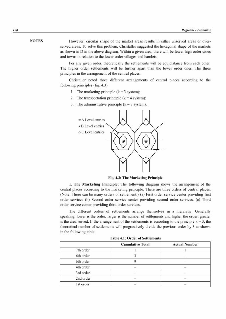
NOTES


However, circular shape of the market areas results in either unserved areas or over-served areas. To solve this problem, Christaller suggested the hexagonal shape of the marketsas shown in D in the above diagram. Within a given area, there will be fewer high order citiesand towns in relation to the lower order villages and hamlets.

For any given order, theoretically the settlements will be equidistance from each other.The higher order settlements will be further apart than the lower order ones. The threeprinciples in the arrangement of the central places:

Christaller noted three different arrangements of central places according to thefollowing principles (fig. 4.3):

1. The marketing principle (k = 3 system);2. The transportation principle (k = 4 system);3. The administrative principle (k = 7 system).

Fig. 4.3: The Marketing Principle

1. The Marketing Principle: The following diagram shows the arrangement of thecentral places according to the marketing principle. There are three orders of central places.(Note: There can be many orders of settlement.) (a) First order service center providing firstorder services (b) Second order service center providing second order services. (c) Thirdorder service center providing third order services.

The different orders of settlements arrange themselves in a hierarchy. Generallyspeaking, lower is the order, larger is the number of settlements and higher the order, greateris the area served. If the arrangement of the settlements is according to the principle k = 3, thetheoretical number of settlements will progressively divide the previous order by 3 as shownin the following table:

Table 4.1: Order of SettlementsCumulative Total Actual Number

7th order 1 16th order 3 –6th order 9 –4th order – –3rd order – –2nd order – –1st order – –

A Level entriesB Level entries

O C Level entries

NOTES


One high order central place is serving three (including itself) of the next lower ordercentral places. The relationship of the market area between a lower order center and thecenters of the higher level can also be indicated by the value 3.

2. The Transportation Principle: Christaller pointed out that the marketing principle isan awkward arrangement in terms of connecting different levels of the hierarchy. As analternate arrangement, Christaller suggested that central places could be organized accordingto what he called the transport principle The traffic principles states that the distribution ofcentral places is most favourable when as many important places as possible lie on one trafficroute between two important towns, the route being established as straightly and as cheap aspossible. The more unimportant places may be left aside. According to the transport principle,the central places would thus be lined up on straight traffic routes which fan out from thecentral point. When central places are arranged according to the traffic principle, the lowerorder centers are located at the midpoint of each side of the hexagon rather than at the corner.Thus, the transport principle produces a hierarchy organized in a k = 4 arrangement in whichcentral places are nested according to the rule of four.

Fig. 4.4: The Transportation Principle

The following table shows how the k = 4 principle can be interpreted:

Table 4.2: Level of Hierarchy Equivalent Number of Central Places

Equivalent Number ofMarker Areas

Dominated by Higher OrderCenter

Dominated by Higher OrderCenter

1. Metropolis 1 1

2. City 3 4

3. Town 12 16

4. Village 48 64

5. Hamlet 192 256

3. The Administrative Principle: Christaller’s other suggested organizing principlewas based upon the realization that from a political or administrative viewpoint centers, itwas unrealistic for centers to be ‘shared’. Any pattern of control which cuts throughfunctional units is potentially problematical. Christaller suggested that an arrangementwhereby lower order centers were entirely with the hexagon of the higher order center wouldobviate such problems. Such a pattern is shown in the following diagram. All the six lowerorder centers are fully subordinate to the higher order center which, therefore, dominates theequivalent of seven market areas at the next lowest level as shown in fig. (4.5).

A Centre

B Centre

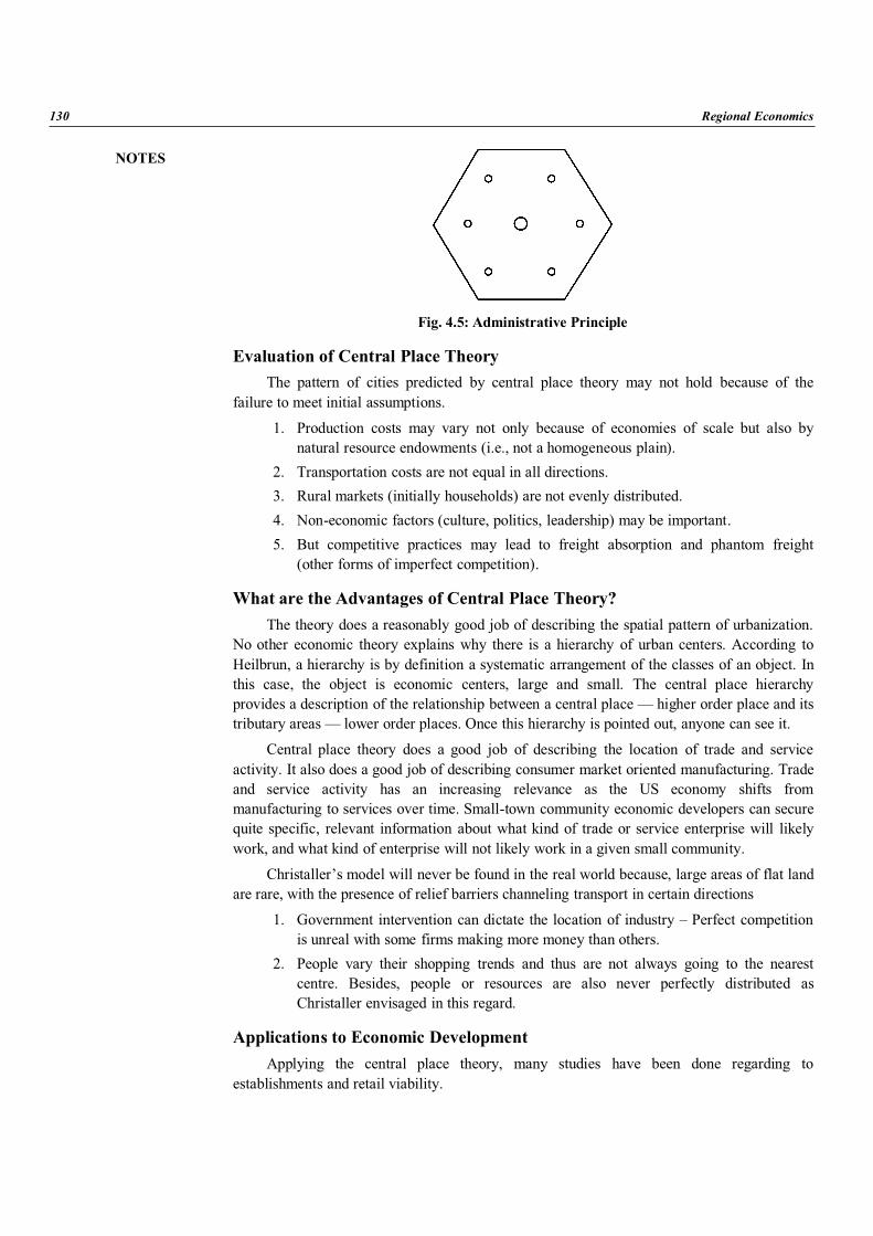
NOTES


Fig. 4.5: Administrative Principle

Evaluation of Central Place TheoryThe pattern of cities predicted by central place theory may not hold because of the

failure to meet initial assumptions.

1. Production costs may vary not only because of economies of scale but also bynatural resource endowments (i.e., not a homogeneous plain).

2. Transportation costs are not equal in all directions.3. Rural markets (initially households) are not evenly distributed.4. Non-economic factors (culture, politics, leadership) may be important.5. But competitive practices may lead to freight absorption and phantom freight

(other forms of imperfect competition).

What are the Advantages of Central Place Theory?The theory does a reasonably good job of describing the spatial pattern of urbanization.

No other economic theory explains why there is a hierarchy of urban centers. According toHeilbrun, a hierarchy is by definition a systematic arrangement of the classes of an object. Inthis case, the object is economic centers, large and small. The central place hierarchyprovides a description of the relationship between a central place — higher order place and itstributary areas — lower order places. Once this hierarchy is pointed out, anyone can see it.

Central place theory does a good job of describing the location of trade and serviceactivity. It also does a good job of describing consumer market oriented manufacturing. Tradeand service activity has an increasing relevance as the US economy shifts frommanufacturing to services over time. Small-town community economic developers can securequite specific, relevant information about what kind of trade or service enterprise will likelywork, and what kind of enterprise will not likely work in a given small community.

Christaller’s model will never be found in the real world because, large areas of flat landare rare, with the presence of relief barriers channeling transport in certain directions

1. Government intervention can dictate the location of industry – Perfect competitionis unreal with some firms making more money than others.

2. People vary their shopping trends and thus are not always going to the nearestcentre. Besides, people or resources are also never perfectly distributed asChristaller envisaged in this regard.

Applications to Economic DevelopmentApplying the central place theory, many studies have been done regarding to

establishments and retail viability.

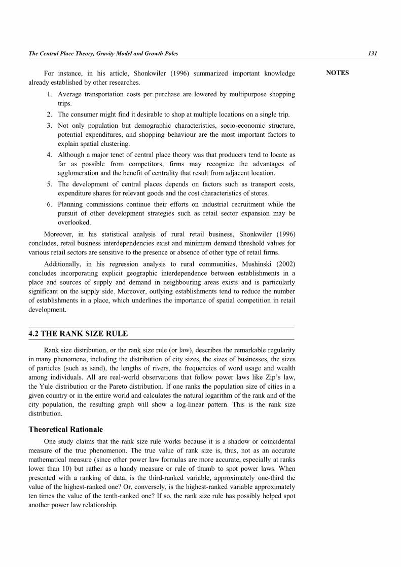
NOTES


For instance, in his article, Shonkwiler (1996) summarized important knowledgealready established by other researches.

1. Average transportation costs per purchase are lowered by multipurpose shoppingtrips.

2. The consumer might find it desirable to shop at multiple locations on a single trip.3. Not only population but demographic characteristics, socio-economic structure,

potential expenditures, and shopping behaviour are the most important factors toexplain spatial clustering.

4. Although a major tenet of central place theory was that producers tend to locate asfar as possible from competitors, firms may recognize the advantages ofagglomeration and the benefit of centrality that result from adjacent location.

5. The development of central places depends on factors such as transport costs,expenditure shares for relevant goods and the cost characteristics of stores.

6. Planning commissions continue their efforts on industrial recruitment while thepursuit of other development strategies such as retail sector expansion may beoverlooked.

Moreover, in his statistical analysis of rural retail business, Shonkwiler (1996)concludes, retail business interdependencies exist and minimum demand threshold values forvarious retail sectors are sensitive to the presence or absence of other type of retail firms.

Additionally, in his regression analysis to rural communities, Mushinski (2002)concludes incorporating explicit geographic interdependence between establishments in aplace and sources of supply and demand in neighbouring areas exists and is particularlysignificant on the supply side. Moreover, outlying establishments tend to reduce the numberof establishments in a place, which underlines the importance of spatial competition in retaildevelopment.

4.2 THE RANK SIZE RULE

Rank size distribution, or the rank size rule (or law), describes the remarkable regularityin many phenomena, including the distribution of city sizes, the sizes of businesses, the sizesof particles (such as sand), the lengths of rivers, the frequencies of word usage and wealthamong individuals. All are real-world observations that follow power laws like Zip’s law,the Yule distribution or the Pareto distribution. If one ranks the population size of cities in agiven country or in the entire world and calculates the natural logarithm of the rank and of thecity population, the resulting graph will show a log-linear pattern. This is the rank sizedistribution.

Theoretical RationaleOne study claims that the rank size rule works because it is a shadow or coincidental

measure of the true phenomenon. The true value of rank size is, thus, not as an accuratemathematical measure (since other power law formulas are more accurate, especially at rankslower than 10) but rather as a handy measure or rule of thumb to spot power laws. Whenpresented with a ranking of data, is the third-ranked variable, approximately one-third thevalue of the highest-ranked one? Or, conversely, is the highest-ranked variable approximatelyten times the value of the tenth-ranked one? If so, the rank size rule has possibly helped spotanother power law relationship.

NOTES


Simple Rank Size DistributionsIn case of city populations, resulting distribution in a country, a region or the world will

be characterized by its largest city, with other cities decreasing in size respective to it,initially at a rapid rate and then more slowly. It results in a few large cities and a much largernumber of cities orders of magnitude smaller. For instance, a rank 3 city would have one-third the population of a country’s largest city, a rank 4 city would have one-fourth thepopulation of the largest city and so on.

While any log-linear factor is ranked, the ranks follow the Lucas numbers, that consistof the sequentially additive numbers 1, 3, 4, 7, 11, 18, 29, 47, 76, 123, 199, etc. Like the morefamous Fibonacci sequence, each number is approximately 1.618 (the Golden ratio) times thepreceding number. For instance, the third term in the sequence above, 4, is approximately1.6183, or 4.236; the fourth term, 7, is approximately 1.6184, or 6.854; the eighth term, 47, isapproximately 1.6188, or 46.979. With higher values, the figures converge. An equiangularspiral is sometimes used to visualize such sequences.

Known Exceptions to Simple Rank Size DistributionsWhile Zipf’s law works well in many cases, it tends to not fit the largest cities in many

countries. A 2002 study found that Zipf’s Law was rejected for 53 of 73 countries, far morethan would be expected based on random chance. The study also found that variations of thePareto exponent are better explained by political variables than by economic geographyvariables like proxies for economies of scale or transportation costs. A 2004 study showedthat Zipf’s law did not work well for the five largest cities in six countries. In the richercountries, the distribution was flatter than predicted. For instance, in the United States,although its largest city, New York City, has more than twice the population of second-place Los Angeles, the two cities’ metropolitan areas (also the two largest in the country) aremuch closer in population. In metropolitan area population, New York City is only 1.3 timeslarger than Los Angeles. In case of other countries, the largest city would dominate muchmore than expected. For instance, in the Democratic Republic of the Congo, thecapital, Kinshasa is more than eight times larger than the second-largest city, Lubumbashi.When considering the entire distribution of cities, including the smallest ones, the rank sizerule does not hold. Instead, the distribution is log-normal. This follows from Gibrat’s law ofproportionate growth.

Because exceptions are so easy to find, the function of the rule for which analyzes citiestoday is to compare the city systems in different nations. The rank size rule is a commonstandard by which urban primacy is established. A distribution such as that in the UnitedStates or China does not exhibit a pattern of primacy, but countries with a dominant primatecity distinctly vary from the rank size rule in the opposite manner. Thus, the rule helps toclassify national (or regional) city systems according to the degree of dominance thatexhibited by the largest city. Countries with a primate city, for example, have typically had acolonial history that accounts for that city pattern. Now, if a normal city distribution pattern isexpected to follow the rank size rule (i.e., if the rank size principle correlates with centralplace theory), then it suggests that those nations or regions with distributions that do notfollow the rule have experienced some conditions that have altered the normal distributionpattern. For instance, the presence of multiple regions within large countries like that ofChina and the United States tends to favour a pattern in which more large cities appear thanwould be predicted by the rule. By contrast, small countries that had been connected (e.g.,colonially or economically) to much larger areas will exhibit a distribution in which the

NOTES


largest city is much larger than would fit the rule, compared with the other cities — theexcessive size of the city theoretically stems from its connection with a larger system ratherthan the natural hierarchy that central place theory would predict within that one country orregion alone.

4.3 GRAVITY MODEL

The gravity model in economics was until relatively recently an intellectual orphan,unconnected to the rich family of economic theory. This review is a tale of the orphan’sreunion with its heritage and the benefits that continue to flow from connections to moredistant relatives.

Gravity has long been one of the most successful empirical models in economics,ordering remarkably well the enormous observed variation in economic interaction acrossspace in both trade and factor movements. The good fit and relatively tight clustering ofcoefficient estimates in the vast empirical literature suggested that some underlying economiclaw must be at work, but in the absence of an accepted connection to economic theory, mosteconomists ignored gravity. The authoritative survey of Leamer and Levinsohn (1995)captures the mid-90’s state of professional thinking: These estimates of gravity have beenboth singularly successful and singularly unsuccessful. They have produced some of theclearest and most robust empirical findings in economics. But, paradoxically, they have hadvirtually no effect on the subject of international economics. Textbooks continue to be writtenand courses designed without any explicit references to distance, but with the very strangeimplicit assumption that countries are both infinitely far apart and infinitely close, the formerreferring to factors and the latter to commodities. Subsequently, gravity first appeared intextbooks in 2004 (Feenstra, 2004), following on success in connecting gravity to economictheory.

Reviews are not intended to be surveys. The gravity model licensed to be idiosyncratic,scants or omits some topics that others have found important while it emphasizes some topicsthat others have scanted. Major emphases and omissions are intended to guide the orphan tomaturity. An adoptive parent’s biases may have contaminated my judgement, caveat emptor,incorporating the theoretical foundations of gravity into recent practice has led to richer andmore accurate estimation and interpretation of the spatial relations described by gravity. Theharvest reaped from empirical work applying the gravity model is recently surveyedelsewhere.

From a modelling standpoint, gravity is distinguished by its parsimonious and tractablerepresentation of economic interaction in a many country world. Most international economictheory is concentrated on two country cases, occasionally extended to three country caseswith special features. The tractability of gravity in the many country case is due to itsmodularity: the distribution of goods or factors across space is determined by gravity forcesconditional on the size of economic activities at each location. Modularity readily allows fordisaggregation by goods or regions at any scale and permits inference about trade costs notdependent on any particular model of production and market structure in full generalequilibrium. The modularity theme recurs often below, but is missing from some otherprominent treatments of gravity in the literature.

NOTES


Traditional GravityThe story begins with setting out the traditional gravity model and noting clues to

uniting it with economic theory. The traditional gravity model drew on analogy withNewton’s Law of Gravitation. A mass of goods or labour or other factors of productionsupplied at origin i, Yi, is attracted to a mass of demand for goods or labour at destination j, Ej,but the potential flow is reduced by distance between them, dij. Strictly applying the analogy,

Xij – YiEj – d2ij

gives the predicted movement of goods or labour between i and j, Xij. Ravensteinpioneered the use of gravity for migration patterns in the 19th century UK. Tinbergen (1962)was the first to use gravity to explain trade flows. Departing from strict analogy, traditionalgravity allowed the coefficients of 1 applied to the mass variables and of 2 applied to bilateraldistance to be generated by data to fit a statistically inferred relationship between data onflows and the mass variables and distance. Generally, across many applications, the estimatedcoefficients on the mass variables cluster close to 1 and the distance coefficients cluster closeto –1 while the estimated equation fits the data very well: most data points cluster close to thefitted line in the sense that 80-90 percent of the variation in the flows is captured by the fittedrelationship. This fitted relationship of traditional gravity improved while supplemented withother proxies for trade frictions, like the effect of political borders, common language and thelike.

Notice that bilateral frictions alone would appear to be inadequate to fully explain theeffects of trade frictions on bilateral trade, because the sale from i to j is influenced by theresistance to movement on i’s other alternative destinations and by the resistance onmovement to j from j’s alternative sources of supply. Prodded by this intuition, the traditionalgravity literature recently developed remoteness indexes of each country’s average effectivedistance to or from its partners idij/Yi was commonly defined as the remoteness of country j)and used them as further explanatory variables in the traditional gravity model, with somestatistical success.

The general problem posed by the intuition behind remoteness indexes is analogous tothe N-body problem in Newtonian gravitation. An economic theory of gravity is required foran adequate solution. Because there are many origins and many destinations in anyapplication, a theory of the bilateral flows must account for the relative attractiveness oforigin-destination pairs. Each sale has multiple possible destinations and each purchase hasmultiple possible origins: any bilateral sale interacts with all others and involves all otherbilateral frictions. This general equilibrium problem is neatly solved with structural gravitymodels. For expositional ease, the discussion will focus on goods movements from now onexcept when migration or investment are specifically treated.

Frictionless Gravity Lessons: Taking a step toward structure, an intuitively appealingstarting point is the description of a completely smooth homogeneous world in which allfrictions disappear. Developing the implications of this structure yields a number of usefulinsights about the pattern of world trade. A frictionless world implies that each good has thesame price everywhere. In a homogeneous world, economic agents everywhere might bepredicted to purchase goods in the same proportions when faced with the same prices. In thenext section, the assumptions on preferences and/or technology that justify this plausibleprediction will be the focus, but here the focus is on what the implications are for tradepatterns. In a completely frictionless and homogeneous world, the natural benchmarkprediction is that Xij / Ej – Yi / Y, the proportion of spending by j on goods from i is equal to

NOTES


the global proportion of spending on goods from i, where Y denotes world spending. Anytheory must impose adding up constraints, which for goods requires that the sum of sales toall destinations must equal Yi, the total sales by origin i, and the sum of purchases from allorigins must equal Ej, the total expenditure for each destination j. Total sales andexpenditures must be equal, i.e.,

i Yi – j Ej – Y

One immediate pay-off is an implication for inferring trade frictions. Multiplying bothsides of the frictionless benchmark prediction, Xi/Ej – Yi/Y by Ej yields predicted frictionlesstrade YiEj/Y. The ratio of observed trade Xij to predicted frictionless trade YiEj/Y representsthe effect of frictions along with random influences. (Bilateral trade data is notoriously rifewith measurement error.) Fitting the statistical relationship between the ratio of observed tofrictionless trade and various proxies for trade costs is justified by this simple theoreticalstructure as a proper focus of empirical gravity models.

Thus far, the treatment of trade flows has been of a generic good which most of theliterature has implemented as an aggregate: the value of aggregate bilateral trade in goods forexample. But the model applies more naturally to disaggregated goods (and factors) becausethe frictions to be analyzed below are likely to differ markedly by product characteristics. Theextension to disaggregated goods, indexed by k, is straightforward.

kki

kik

kjj

ijk Ybs

Y

EY X

..... (1)

Here, ski – Yki /Yk is country i’s share of the world’s sales of goods class k andbki – Ekj/Yk is country j’s share of the world spending on k, equal to world sales of k, Yk.

The notation and logic also readily apply to disaggregation of countries into regions andindeed a prominent portion of the empirical literature has examined bilateral flows betweencity pairs or regions, motivated by the observation that much economic interaction isconcentrated at very short distances in aggregate gravity applications (i.e., most applications),it has been common to use origin and destination mass variables equal to Gross DomesticProduct (GDP). This is conceptually inappropriate and leads to inaccurate modelling unlessthe ratio of gross shipments to GDP is constant (in which case the ratio goes into a constantterm). A possible direction for aggregate modelling is to convert trade to the same valueadded basis as GDP, but this seems more problematic than using disaggregated gravity toexplain the pattern of gross shipments and then uniting estimated gravity models within asuperstructure to connect to GDP. That is the strategy of the structural gravity model researchprogram reviewed here. Equation (1) generates a number of useful implications:

1. big producers have big market shares everywhere,2. small sellers are more open in the sense of trading more with the rest of the world,3. the world is more open the more similar in size are countries and the more

specialized are countries,4. the world is more open the greater the number of countries, and5. world openness rises with convergence under the simplifying assumption of

balanced trade.

As for implication 1 big producers have big market shares everywhere, this followsbecause, reverting to the generic notation and omitting the k superscript, the frictionlessgravity prediction is that:

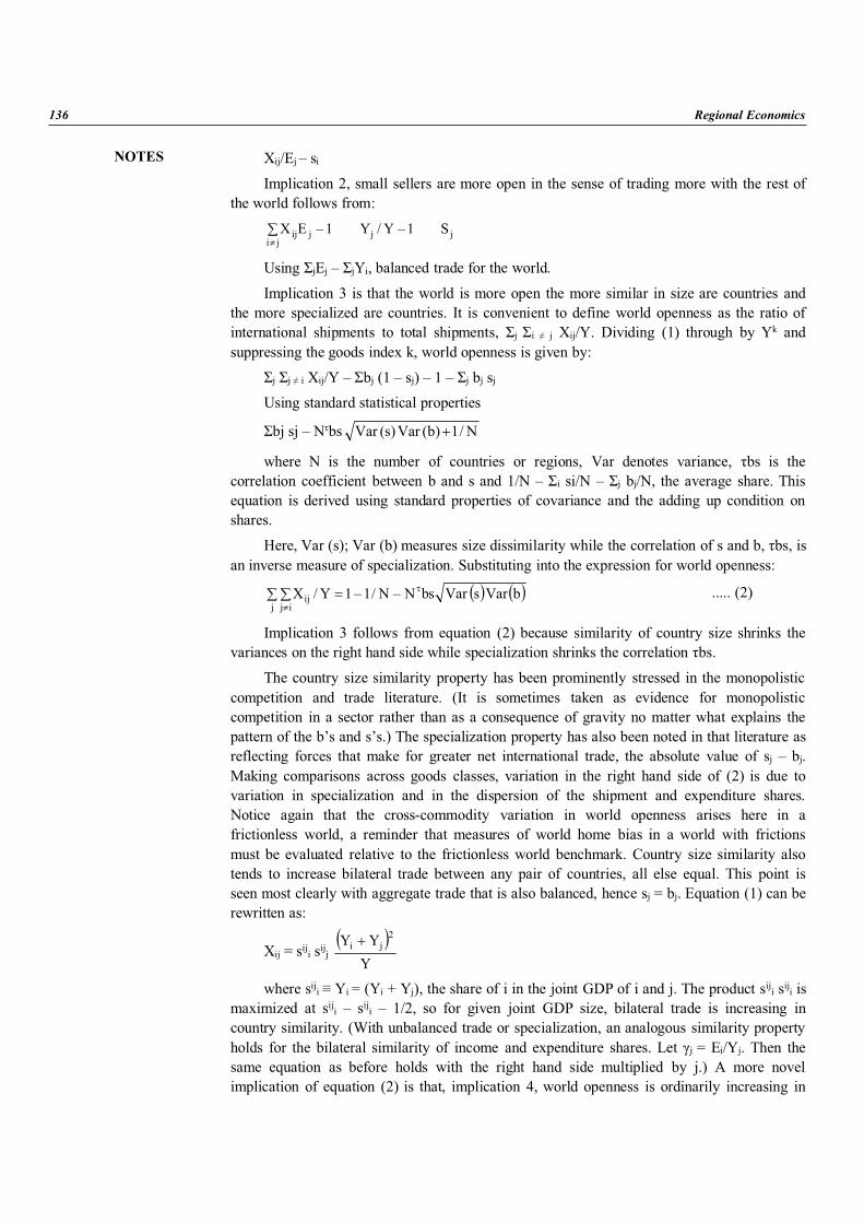
NOTES


Xij/Ej – si

Implication 2, small sellers are more open in the sense of trading more with the rest ofthe world follows from:

jji

jjij S1–Y/Y1–EX

Using jEj – jYi, balanced trade for the world.

Implication 3 is that the world is more open the more similar in size are countries andthe more specialized are countries. It is convenient to define world openness as the ratio ofinternational shipments to total shipments, j i j Xij/Y. Dividing (1) through by Yk andsuppressing the goods index k, world openness is given by:

j j i Xij/Y – bj (1 – sj) – 1 – j bj sj

Using standard statistical properties

bj sj – N bs N/1)b(Var)s(Var

where N is the number of countries or regions, Var denotes variance, bs is thecorrelation coefficient between b and s and 1/N – i si/N – j bj/N, the average share. Thisequation is derived using standard properties of covariance and the adding up condition onshares.

Here, Var (s); Var (b) measures size dissimilarity while the correlation of s and b, bs, isan inverse measure of specialization. Substituting into the expression for world openness:

j ijij bVarsVarbsN–N/1–1Y/X ..... (2)

Implication 3 follows from equation (2) because similarity of country size shrinks thevariances on the right hand side while specialization shrinks the correlation bs.

The country size similarity property has been prominently stressed in the monopolisticcompetition and trade literature. (It is sometimes taken as evidence for monopolisticcompetition in a sector rather than as a consequence of gravity no matter what explains thepattern of the b’s and s’s.) The specialization property has also been noted in that literature asreflecting forces that make for greater net international trade, the absolute value of sj – bj.Making comparisons across goods classes, variation in the right hand side of (2) is due tovariation in specialization and in the dispersion of the shipment and expenditure shares.Notice again that the cross-commodity variation in world openness arises here in africtionless world, a reminder that measures of world home bias in a world with frictionsmust be evaluated relative to the frictionless world benchmark. Country size similarity alsotends to increase bilateral trade between any pair of countries, all else equal. This point isseen most clearly with aggregate trade that is also balanced, hence sj = bj. Equation (1) can berewritten as:

Xij = siji sijjY

YY 2ji

where siji Yi = (Yi + Yj), the share of i in the joint GDP of i and j. The product siji siji ismaximized at siji – siji – 1/2, so for given joint GDP size, bilateral trade is increasing incountry similarity. (With unbalanced trade or specialization, an analogous similarity propertyholds for the bilateral similarity of income and expenditure shares. Let j = Ei/Yj. Then thesame equation as before holds with the right hand side multiplied by j.) A more novelimplication of equation (2) is that, implication 4, world openness is ordinarily increasing in

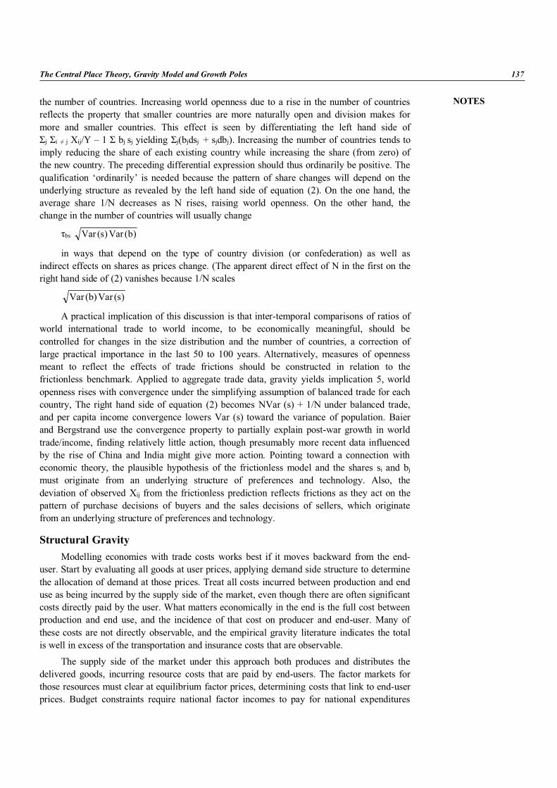
NOTES


the number of countries. Increasing world openness due to a rise in the number of countriesreflects the property that smaller countries are more naturally open and division makes formore and smaller countries. This effect is seen by differentiating the left hand side of

j i j Xij/Y – 1 bj sj yielding j(bjdsj + sjdbj). Increasing the number of countries tends toimply reducing the share of each existing country while increasing the share (from zero) ofthe new country. The preceding differential expression should thus ordinarily be positive. Thequalification ‘ordinarily’ is needed because the pattern of share changes will depend on theunderlying structure as revealed by the left hand side of equation (2). On the one hand, theaverage share 1/N decreases as N rises, raising world openness. On the other hand, thechange in the number of countries will usually change

bs )b(Var)s(Var

in ways that depend on the type of country division (or confederation) as well asindirect effects on shares as prices change. (The apparent direct effect of N in the first on theright hand side of (2) vanishes because 1/N scales

)s(Var)b(Var

A practical implication of this discussion is that inter-temporal comparisons of ratios ofworld international trade to world income, to be economically meaningful, should becontrolled for changes in the size distribution and the number of countries, a correction oflarge practical importance in the last 50 to 100 years. Alternatively, measures of opennessmeant to reflect the effects of trade frictions should be constructed in relation to thefrictionless benchmark. Applied to aggregate trade data, gravity yields implication 5, worldopenness rises with convergence under the simplifying assumption of balanced trade for eachcountry, The right hand side of equation (2) becomes NVar (s) + 1/N under balanced trade,and per capita income convergence lowers Var (s) toward the variance of population. Baierand Bergstrand use the convergence property to partially explain post-war growth in worldtrade/income, finding relatively little action, though presumably more recent data influencedby the rise of China and India might give more action. Pointing toward a connection witheconomic theory, the plausible hypothesis of the frictionless model and the shares si and bj

must originate from an underlying structure of preferences and technology. Also, thedeviation of observed Xij from the frictionless prediction reflects frictions as they act on thepattern of purchase decisions of buyers and the sales decisions of sellers, which originatefrom an underlying structure of preferences and technology.

Structural GravityModelling economies with trade costs works best if it moves backward from the end-

user. Start by evaluating all goods at user prices, applying demand side structure to determinethe allocation of demand at those prices. Treat all costs incurred between production and enduse as being incurred by the supply side of the market, even though there are often significantcosts directly paid by the user. What matters economically in the end is the full cost betweenproduction and end use, and the incidence of that cost on producer and end-user. Many ofthese costs are not directly observable, and the empirical gravity literature indicates the totalis well in excess of the transportation and insurance costs that are observable.

The supply side of the market under this approach both produces and distributes thedelivered goods, incurring resource costs that are paid by end-users. The factor markets forthose resources must clear at equilibrium factor prices, determining costs that link to end-userprices. Budget constraints require national factor incomes to pay for national expenditures

NOTES


plus net lending or transfers including remittances. Below the national accounts, individualeconomic agents also meet budget constraints. Goods markets clear when prices are foundsuch that demand is equal to supply for each good. The full general equilibrium requires a setof bilateral factor prices and bilateral goods prices such that all markets clear and all budgetconstraints are met.

This standard description of general economic equilibrium is too complex to yieldsomething like gravity. A hugely useful simplification is modularity, subordinating theeconomic determination of equilibrium distribution of goods within a class under thesuperstructure determination of distribution of production and expenditure between classes ofgoods. Anderson and van Wincoop call this property trade separability. Observing that goodsare typically supplied from multiple locations, even within fine census commodity classes, itis natural to look for a theoretical structure that justifies grouping in this way. The structuralgravity model literature has uncovered two structures that work, one on the demand side andone on the supply side.

Modularity (trade separability) permits the analyst to focus exclusively on inferenceabout distribution costs from the pattern of distribution of goods (or factors) without havingto explain at the same time what determines the total supplies of goods to all destinations orthe total demand for goods from all origins. This is a great advantage for two reasons. First, itsimplifies the inference task enormously. Second, the inferences about the distribution ofgoods or factors is consistent with a great many plausible general equilibrium models ofnational (or regional) production and consumption. Modularity also requires a restriction ontrade costs, so that only the national aggregate burden of trade costs within a goods classmatters for allocation between classes. The most popular way to meet this requirement is torestrict the trade costs so that the distribution of goods uses resources in the same proportionas the production of those same goods. Samuelson (1952) invented iceberg melting tradecosts in which the trade costs were proportional to the volume shipped, as the amount meltedfrom the iceberg is proportional to its volume.

The iceberg metaphor still applies when allowing for a fixed cost, as if a chunk of theiceberg breaks off as it parts from the mother glacier. Mathematically, the generalized icebergtrade cost is linear in the volume shipped. Economically, distribution continues to requireresources to be used in the same proportion as in production. Fixed costs are realistic andpotentially play an important role in explaining why many potential bilateral flows are equalto zero. More general non-linear trade cost functions continue to satisfy the productionproportionality restriction and thus meet the requirements of modularity, but depart from theiceberg metaphor. Bergstrand derived a joint cost function that is homogeneous of degree onewith Constant Elasticity of Transformation (CET). This setup allows for substitution effectsin costs between destinations rather than the cost independence due to fixed coefficients inthe iceberg model. Bilateral costs have a natural aggregator that is an iceberg cost facingmonopolistically competitive firms. A nice feature of the joint cost model is its econometrictractability under the hypothesis of profit maximizing choice of destinations. Whilepotentially more realistic, the joint cost refinement turns out to make relatively littledifference empirically.

Arkolakis (2008) develops a non-linear (in volume) trade cost function in whichheterogeneous customers are obtained by firms with a marketing technology featuring a fixedcost component (running a national advertisement) and a variable cost component (leaflettingor telemarketing) subject to diminishing returns as the less likely customers are encountered.Because of the Ricardian production and distribution technology, resource requirements in

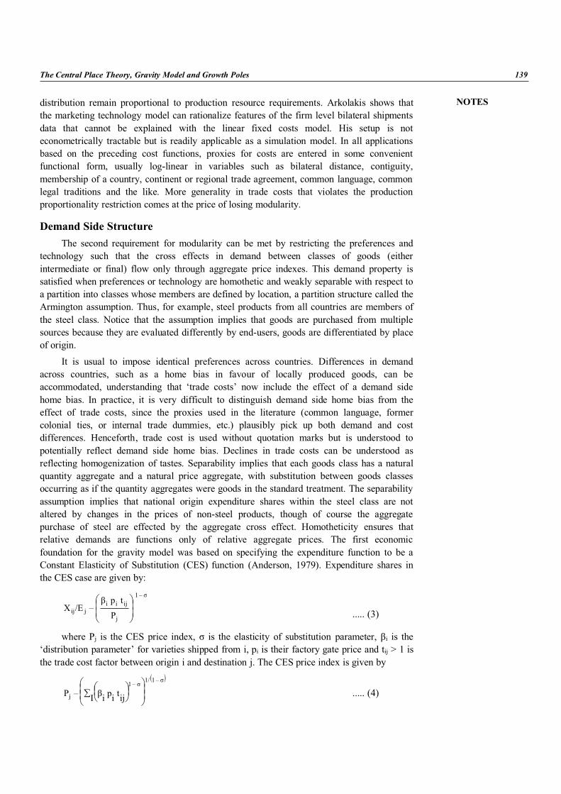
NOTES


distribution remain proportional to production resource requirements. Arkolakis shows thatthe marketing technology model can rationalize features of the firm level bilateral shipmentsdata that cannot be explained with the linear fixed costs model. His setup is noteconometrically tractable but is readily applicable as a simulation model. In all applicationsbased on the preceding cost functions, proxies for costs are entered in some convenientfunctional form, usually log-linear in variables such as bilateral distance, contiguity,membership of a country, continent or regional trade agreement, common language, commonlegal traditions and the like. More generality in trade costs that violates the productionproportionality restriction comes at the price of losing modularity.

Demand Side StructureThe second requirement for modularity can be met by restricting the preferences and

technology such that the cross effects in demand between classes of goods (eitherintermediate or final) flow only through aggregate price indexes. This demand property issatisfied when preferences or technology are homothetic and weakly separable with respect toa partition into classes whose members are defined by location, a partition structure called theArmington assumption. Thus, for example, steel products from all countries are members ofthe steel class. Notice that the assumption implies that goods are purchased from multiplesources because they are evaluated differently by end-users, goods are differentiated by placeof origin.

It is usual to impose identical preferences across countries. Differences in demandacross countries, such as a home bias in favour of locally produced goods, can beaccommodated, understanding that ‘trade costs’ now include the effect of a demand sidehome bias. In practice, it is very difficult to distinguish demand side home bias from theeffect of trade costs, since the proxies used in the literature (common language, formercolonial ties, or internal trade dummies, etc.) plausibly pick up both demand and costdifferences. Henceforth, trade cost is used without quotation marks but is understood topotentially reflect demand side home bias. Declines in trade costs can be understood asreflecting homogenization of tastes. Separability implies that each goods class has a naturalquantity aggregate and a natural price aggregate, with substitution between goods classesoccurring as if the quantity aggregates were goods in the standard treatment. The separabilityassumption implies that national origin expenditure shares within the steel class are notaltered by changes in the prices of non-steel products, though of course the aggregatepurchase of steel are effected by the aggregate cross effect. Homotheticity ensures thatrelative demands are functions only of relative aggregate prices. The first economicfoundation for the gravity model was based on specifying the expenditure function to be aConstant Elasticity of Substitution (CES) function (Anderson, 1979). Expenditure shares inthe CES case are given by:

– 1

j

ijiijij P

tp –/EX ..... (3)

where Pj is the CES price index, is the elasticity of substitution parameter, i is the‘distribution parameter’ for varieties shipped from i, pi is their factory gate price and tij > 1 isthe trade cost factor between origin i and destination j. The CES price index is given by

– 11/– 1

j ij tip iI –P ..... (4)

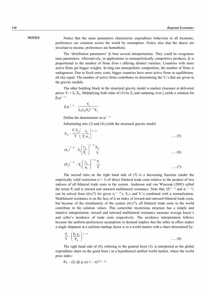
NOTES


Notice that the same parameters characterize expenditure behaviour in all locations;preferences are common across the world by assumption. Notice also that the shares areinvariant to income, preferences are homothetic.

The ‘distribution parameters’ i bear several interpretations. They could be exogenoustaste parameters. Alternatively, in applications to monopolistically competitive products, i isproportional to the number of firms from i offering distinct varieties. Countries with moreactive firms get bigger weights. In long-run monopolistic competition, the number of firms isendogenous. Due to fixed entry costs, bigger countries have more active firms in equilibrium,all else equal. The number of active firms contributes to determining the Yi’s that are given inthe gravity module.

The other building block in the structural gravity model is market clearance at deliveredprices Yi = j Xij. Multiplying both sides of (3) by Ej and summing over j yields a solution for

i pi1 –

j– 1

jijJ

i– 1ii

E)/P(t

Y – p

Define the denominator as i1 –

Substituting into (3) and (4) yields the structural gravity model:

– 1

ij

ijjij

P

t

YiYE

–X..... (5)

YE

P t ij

– 1

j

ijj–

– 1i )(

..... (6)

YY

t

–)(P i– 1

i

iji

– 1j ..... (7)

The second ratio on the right hand side of (5) is a decreasing function (under theempirically valid restriction > 1) of direct bilateral trade costs relative to the product of twoindexes of all bilateral trade costs in the system. Anderson and van Wincoop (2003) calledthe terms Pj and i inward and outward multilateral resistance. Note that {Pj1 – and i 1 – }can be solved from (6)-(7) for given tij1 – ’s, Ej’s and Yi’s combined with a normalization.Multilateral resistance is on the face of it an index of inward and outward bilateral trade costs,but because of the simultaneity of the system (6)-(7), all bilateral trade costs in the worldcontribute to the solution values. This somewhat mysterious structure has a simple andintuitive interpretation: inward and outward multilateral resistance measure average buyer’sand seller’s incidence of trade costs respectively. The incidence interpretation followsbecause the uniform preferences assumption in demand implies that the seller in effect makesa single shipment at a uniform markup factor i to a world market with a share determined by:

– 1

w

iii p

–YY

P ..... (8)

The right hand side of (8), referring to the general form (3), is interpreted as the globalexpenditure share on the good from i in a hypothetical unified world market, where the worldprice index:

PW – ( i ( i pi i) 1 – )1/(1 – )

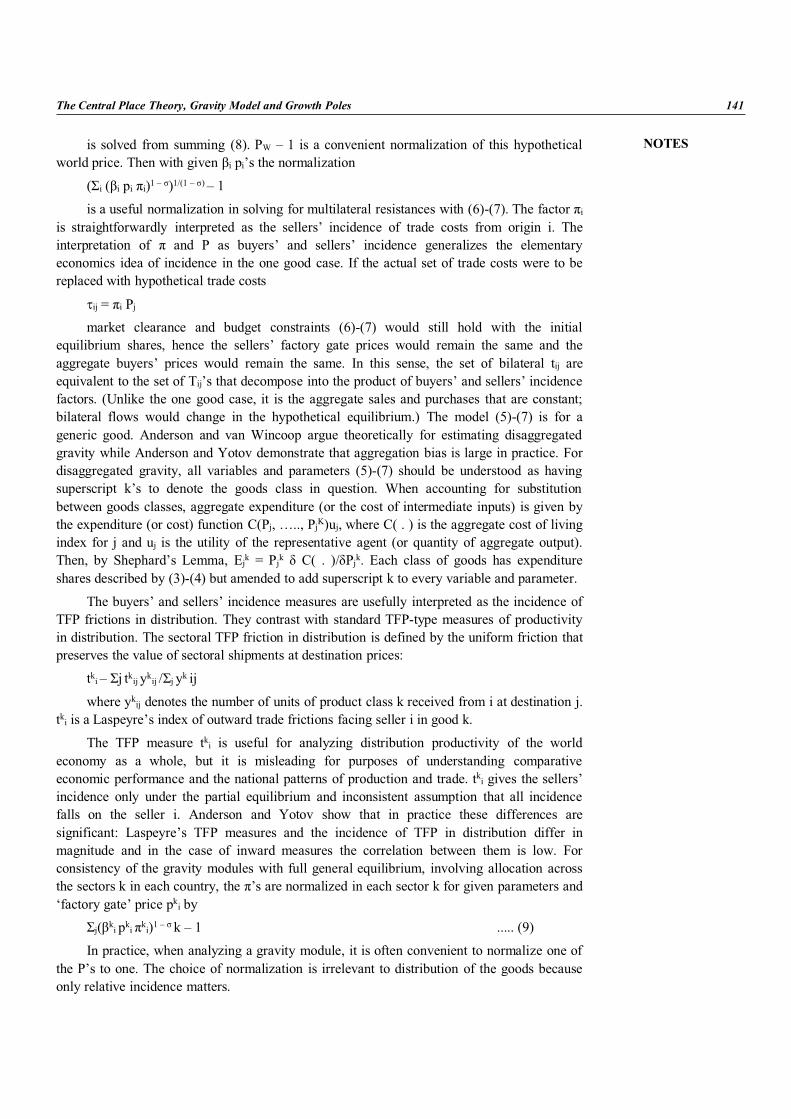
NOTES


is solved from summing (8). PW – 1 is a convenient normalization of this hypotheticalworld price. Then with given i pi’s the normalization

( i ( i pi i)1 – )1/(1 – ) – 1

is a useful normalization in solving for multilateral resistances with (6)-(7). The factor i

is straightforwardly interpreted as the sellers’ incidence of trade costs from origin i. Theinterpretation of and P as buyers’ and sellers’ incidence generalizes the elementaryeconomics idea of incidence in the one good case. If the actual set of trade costs were to bereplaced with hypothetical trade costs

ij = i Pj

market clearance and budget constraints (6)-(7) would still hold with the initialequilibrium shares, hence the sellers’ factory gate prices would remain the same and theaggregate buyers’ prices would remain the same. In this sense, the set of bilateral tij areequivalent to the set of Tij’s that decompose into the product of buyers’ and sellers’ incidencefactors. (Unlike the one good case, it is the aggregate sales and purchases that are constant;bilateral flows would change in the hypothetical equilibrium.) The model (5)-(7) is for ageneric good. Anderson and van Wincoop argue theoretically for estimating disaggregatedgravity while Anderson and Yotov demonstrate that aggregation bias is large in practice. Fordisaggregated gravity, all variables and parameters (5)-(7) should be understood as havingsuperscript k’s to denote the goods class in question. When accounting for substitutionbetween goods classes, aggregate expenditure (or the cost of intermediate inputs) is given bythe expenditure (or cost) function C(Pj, ….., PjK)uj, where C( . ) is the aggregate cost of livingindex for j and uj is the utility of the representative agent (or quantity of aggregate output).Then, by Shephard’s Lemma, Ejk = Pjk C( . )/ Pjk. Each class of goods has expenditureshares described by (3)-(4) but amended to add superscript k to every variable and parameter.

The buyers’ and sellers’ incidence measures are usefully interpreted as the incidence ofTFP frictions in distribution. They contrast with standard TFP-type measures of productivityin distribution. The sectoral TFP friction in distribution is defined by the uniform friction thatpreserves the value of sectoral shipments at destination prices:

tki – j tkij ykij / j yk ij

where ykij denotes the number of units of product class k received from i at destination j.tki is a Laspeyre’s index of outward trade frictions facing seller i in good k.

The TFP measure tki is useful for analyzing distribution productivity of the worldeconomy as a whole, but it is misleading for purposes of understanding comparativeeconomic performance and the national patterns of production and trade. tki gives the sellers’incidence only under the partial equilibrium and inconsistent assumption that all incidencefalls on the seller i. Anderson and Yotov show that in practice these differences aresignificant: Laspeyre’s TFP measures and the incidence of TFP in distribution differ inmagnitude and in the case of inward measures the correlation between them is low. Forconsistency of the gravity modules with full general equilibrium, involving allocation acrossthe sectors k in each country, the ’s are normalized in each sector k for given parameters and‘factory gate’ price pki by

j( ki pki ki)1 – k – 1 ..... (9)

In practice, when analyzing a gravity module, it is often convenient to normalize one ofthe P’s to one. The choice of normalization is irrelevant to distribution of the goods becauseonly relative incidence matters.

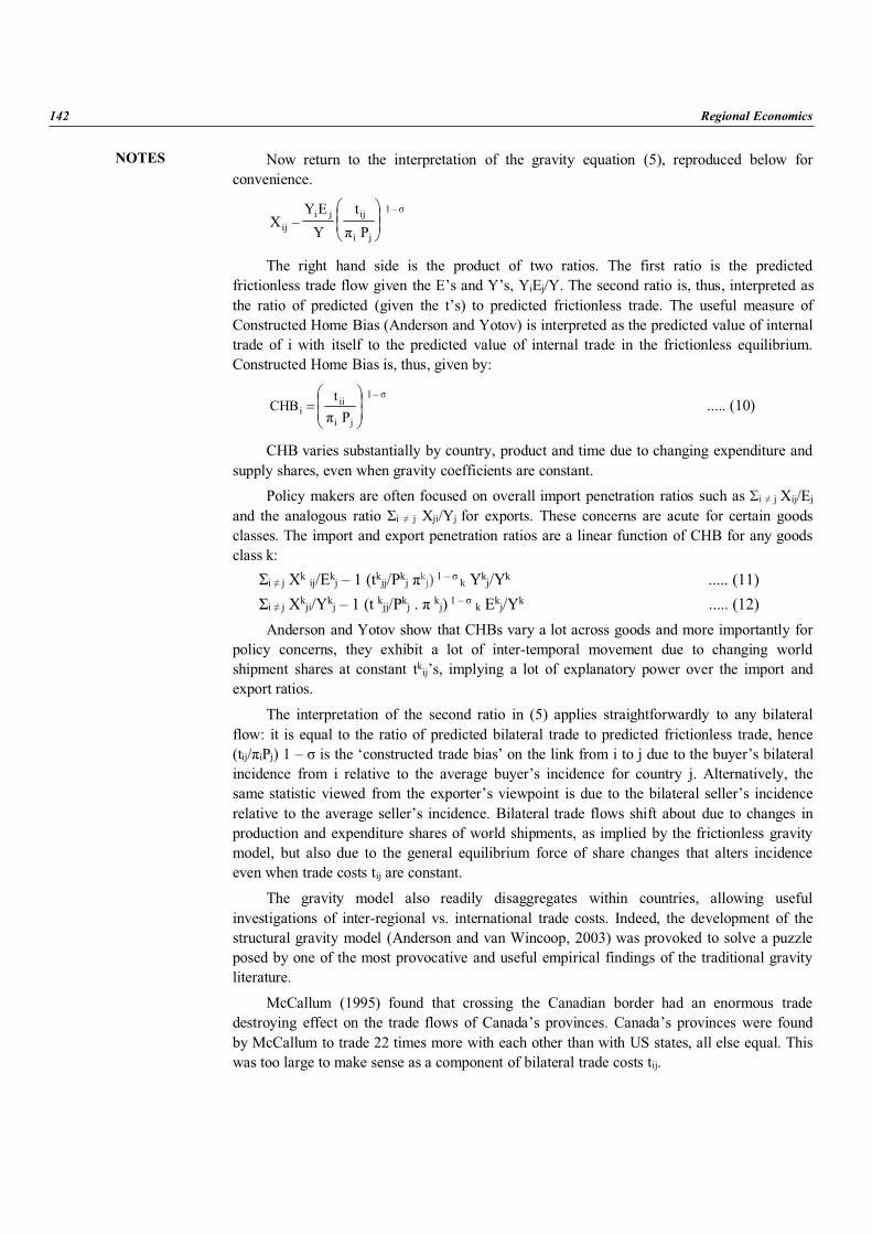
NOTES


Now return to the interpretation of the gravity equation (5), reproduced below forconvenience.

– 1

ji

ijjiij

P t

YEY

– X

The right hand side is the product of two ratios. The first ratio is the predictedfrictionless trade flow given the E’s and Y’s, YiEj/Y. The second ratio is, thus, interpreted asthe ratio of predicted (given the t’s) to predicted frictionless trade. The useful measure ofConstructed Home Bias (Anderson and Yotov) is interpreted as the predicted value of internaltrade of i with itself to the predicted value of internal trade in the frictionless equilibrium.Constructed Home Bias is, thus, given by:

– 1

ji

iii

t CHB

P ..... (10)

CHB varies substantially by country, product and time due to changing expenditure andsupply shares, even when gravity coefficients are constant.

Policy makers are often focused on overall import penetration ratios such as i j Xij/Ej

and the analogous ratio i j Xji/Yj for exports. These concerns are acute for certain goodsclasses. The import and export penetration ratios are a linear function of CHB for any goodsclass k:

i j Xk ij/Ekj – 1 (tkjj/Pkj kj) 1 – k Ykj/Yk ..... (11)i j Xkji/Ykj – 1 (t kjj/Pkj . kj) 1 – k Ekj/Yk ..... (12)Anderson and Yotov show that CHBs vary a lot across goods and more importantly for

policy concerns, they exhibit a lot of inter-temporal movement due to changing worldshipment shares at constant tkij’s, implying a lot of explanatory power over the import andexport ratios.

The interpretation of the second ratio in (5) applies straightforwardly to any bilateralflow: it is equal to the ratio of predicted bilateral trade to predicted frictionless trade, hence(tij/ iPj) 1 – is the ‘constructed trade bias’ on the link from i to j due to the buyer’s bilateralincidence from i relative to the average buyer’s incidence for country j. Alternatively, thesame statistic viewed from the exporter’s viewpoint is due to the bilateral seller’s incidencerelative to the average seller’s incidence. Bilateral trade flows shift about due to changes inproduction and expenditure shares of world shipments, as implied by the frictionless gravitymodel, but also due to the general equilibrium force of share changes that alters incidenceeven when trade costs tij are constant.

The gravity model also readily disaggregates within countries, allowing usefulinvestigations of inter-regional vs. international trade costs. Indeed, the development of thestructural gravity model (Anderson and van Wincoop, 2003) was provoked to solve a puzzleposed by one of the most provocative and useful empirical findings of the traditional gravityliterature.

McCallum (1995) found that crossing the Canadian border had an enormous tradedestroying effect on the trade flows of Canada’s provinces. Canada’s provinces were foundby McCallum to trade 22 times more with each other than with US states, all else equal. Thiswas too large to make sense as a component of bilateral trade costs tij.

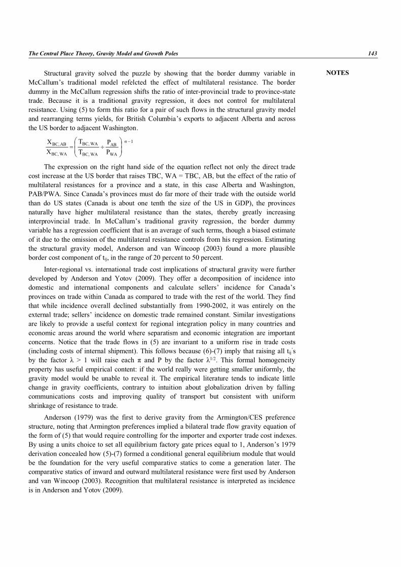
NOTES


Structural gravity solved the puzzle by showing that the border dummy variable inMcCallum’s traditional model refelcted the effect of multilateral resistance. The borderdummy in the McCallum regression shifts the ratio of inter-provincial trade to province-statetrade. Because it is a traditional gravity regression, it does not control for multilateralresistance. Using (5) to form this ratio for a pair of such flows in the structural gravity modeland rearranging terms yields, for British Columbia’s exports to adjacent Alberta and acrossthe US border to adjacent Washington.

1–

WA

AB

WABC,

WABC,

WABC,

AB BC, XX

PP

TT

The expression on the right hand side of the equation reflect not only the direct tradecost increase at the US border that raises TBC, WA = TBC, AB, but the effect of the ratio ofmultilateral resistances for a province and a state, in this case Alberta and Washington,PAB/PWA. Since Canada’s provinces must do far more of their trade with the outside worldthan do US states (Canada is about one tenth the size of the US in GDP), the provincesnaturally have higher multilateral resistance than the states, thereby greatly increasinginterprovincial trade. In McCallum’s traditional gravity regression, the border dummyvariable has a regression coefficient that is an average of such terms, though a biased estimateof it due to the omission of the multilateral resistance controls from his regression. Estimatingthe structural gravity model, Anderson and van Wincoop (2003) found a more plausibleborder cost component of tij, in the range of 20 percent to 50 percent.

Inter-regional vs. international trade cost implications of structural gravity were furtherdeveloped by Anderson and Yotov (2009). They offer a decomposition of incidence intodomestic and international components and calculate sellers’ incidence for Canada’sprovinces on trade within Canada as compared to trade with the rest of the world. They findthat while incidence overall declined substantially from 1990-2002, it was entirely on theexternal trade; sellers’ incidence on domestic trade remained constant. Similar investigationsare likely to provide a useful context for regional integration policy in many countries andeconomic areas around the world where separatism and economic integration are importantconcerns. Notice that the trade flows in (5) are invariant to a uniform rise in trade costs(including costs of internal shipment). This follows because (6)-(7) imply that raising all tij’sby the factor > 1 will raise each and P by the factor 1/2. This formal homogeneityproperty has useful empirical content: if the world really were getting smaller uniformly, thegravity model would be unable to reveal it. The empirical literature tends to indicate littlechange in gravity coefficients, contrary to intuition about globalization driven by fallingcommunications costs and improving quality of transport but consistent with uniformshrinkage of resistance to trade.

Anderson (1979) was the first to derive gravity from the Armington/CES preferencestructure, noting that Armington preferences implied a bilateral trade flow gravity equation ofthe form of (5) that would require controlling for the importer and exporter trade cost indexes.By using a units choice to set all equilibrium factory gate prices equal to 1, Anderson’s 1979derivation concealed how (5)-(7) formed a conditional general equilibrium module that wouldbe the foundation for the very useful comparative statics to come a generation later. Thecomparative statics of inward and outward multilateral resistance were first used by Andersonand van Wincoop (2003). Recognition that multilateral resistance is interpreted as incidenceis in Anderson and Yotov (2009).

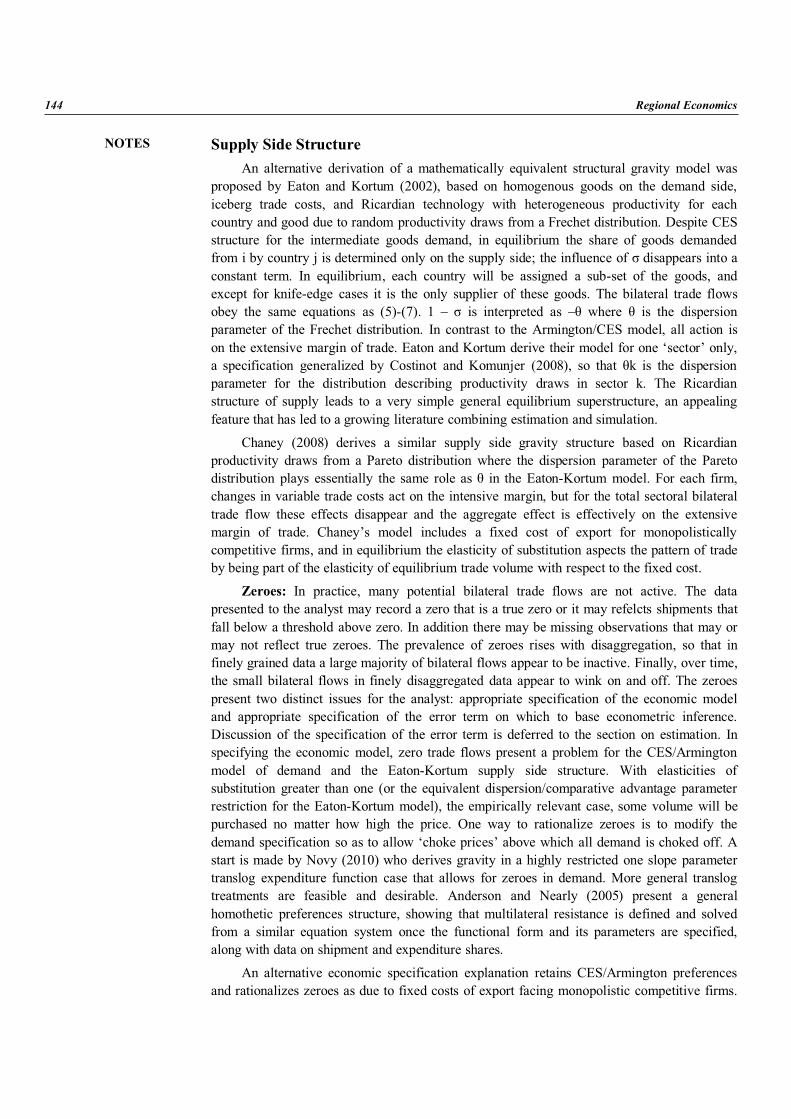
NOTES


Supply Side StructureAn alternative derivation of a mathematically equivalent structural gravity model was

proposed by Eaton and Kortum (2002), based on homogenous goods on the demand side,iceberg trade costs, and Ricardian technology with heterogeneous productivity for eachcountry and good due to random productivity draws from a Frechet distribution. Despite CESstructure for the intermediate goods demand, in equilibrium the share of goods demandedfrom i by country j is determined only on the supply side; the influence of disappears into aconstant term. In equilibrium, each country will be assigned a sub-set of the goods, andexcept for knife-edge cases it is the only supplier of these goods. The bilateral trade flowsobey the same equations as (5)-(7). 1 – is interpreted as – where is the dispersionparameter of the Frechet distribution. In contrast to the Armington/CES model, all action ison the extensive margin of trade. Eaton and Kortum derive their model for one ‘sector’ only,a specification generalized by Costinot and Komunjer (2008), so that k is the dispersionparameter for the distribution describing productivity draws in sector k. The Ricardianstructure of supply leads to a very simple general equilibrium superstructure, an appealingfeature that has led to a growing literature combining estimation and simulation.

Chaney (2008) derives a similar supply side gravity structure based on Ricardianproductivity draws from a Pareto distribution where the dispersion parameter of the Paretodistribution plays essentially the same role as in the Eaton-Kortum model. For each firm,changes in variable trade costs act on the intensive margin, but for the total sectoral bilateraltrade flow these effects disappear and the aggregate effect is effectively on the extensivemargin of trade. Chaney’s model includes a fixed cost of export for monopolisticallycompetitive firms, and in equilibrium the elasticity of substitution aspects the pattern of tradeby being part of the elasticity of equilibrium trade volume with respect to the fixed cost.

Zeroes: In practice, many potential bilateral trade flows are not active. The datapresented to the analyst may record a zero that is a true zero or it may refelcts shipments thatfall below a threshold above zero. In addition there may be missing observations that may ormay not reflect true zeroes. The prevalence of zeroes rises with disaggregation, so that infinely grained data a large majority of bilateral flows appear to be inactive. Finally, over time,the small bilateral flows in finely disaggregated data appear to wink on and off. The zeroespresent two distinct issues for the analyst: appropriate specification of the economic modeland appropriate specification of the error term on which to base econometric inference.Discussion of the specification of the error term is deferred to the section on estimation. Inspecifying the economic model, zero trade flows present a problem for the CES/Armingtonmodel of demand and the Eaton-Kortum supply side structure. With elasticities ofsubstitution greater than one (or the equivalent dispersion/comparative advantage parameterrestriction for the Eaton-Kortum model), the empirically relevant case, some volume will bepurchased no matter how high the price. One way to rationalize zeroes is to modify thedemand specification so as to allow ‘choke prices’ above which all demand is choked off. Astart is made by Novy (2010) who derives gravity in a highly restricted one slope parametertranslog expenditure function case that allows for zeroes in demand. More general translogtreatments are feasible and desirable. Anderson and Nearly (2005) present a generalhomothetic preferences structure, showing that multilateral resistance is defined and solvedfrom a similar equation system once the functional form and its parameters are specified,along with data on shipment and expenditure shares.

An alternative economic specification explanation retains CES/Armington preferencesand rationalizes zeroes as due to fixed costs of export facing monopolistic competitive firms.

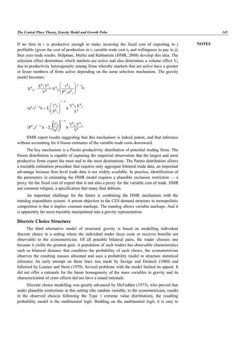
NOTES


If no firm in i is productive enough to make incurring the fixed cost of exporting to jprofitable (given the cost of production in i, variable trade cost tij and willingness to pay in j),then zero trade results. Helpman, Melitz and Rubinstein (HMR, 2008) develop this idea. Theselection effect determines which markets are active and also determines a volume effect Vij

due to productivity heterogeneity among firms whereby markets that are active have a greateror lesser numbers of firms active depending on the same selection mechanism. The gravitymodel becomes:

k Y

Y E– X

– 1

ik

jk

ijk

ijk

ki

kjk

ijk

Pt

V

kjk

ijk

– 1

jkijk

j– 1

ik

Y E Vk

Pt k)( –

kj

kij

k– 1

ikijk

I– 1

jk

Y Y V

kt

–k )(P

HMR report results suggesting that this mechanism is indeed potent, and that inferencewithout accounting for it biases estimates of the variable trade costs downward.

The key mechanism is a Pareto productivity distribution of potential trading firms. ThePareto distribution is capable of capturing the empirical observation that the largest and mostproductive firms export the most and to the most destinations. The Pareto distribution allowsa tractable estimation procedure that requires only aggregate bilateral trade data, an importantadvantage because firm level trade data is not widely available. In practice, identification ofthe parameters in estimating the HMR model requires a plausible exclusion restriction — aproxy for the fixed cost of export that is not also a proxy for the variable cost of trade. HMRuse common religion, a specification that many find dubious.

An important challenge for the future is combining the HMR mechanism with thetranslog expenditure system. A potent objection to the CES demand structure in monopolisticcompetition is that it implies constant markups. The translog allows variable markups. And itis apparently far more tractably manipulated into a gravity representation.

Discrete Choice StructureThe third alternative model of structural gravity is based on modelling individual

discrete choice in a setting where the individual trader faces costs or receives benefits notobservable to the econometrician. Of all possible bilateral pairs, the trader chooses onebecause it yields the greatest gain. A population of such traders has observable characteristicssuch as bilateral distance that condition the probability of each choice, the econometricianobserves the resulting masses allocated and uses a probability model to structure statisticalinference An early attempt on these lines was made by Savage and Deutsch (1960) andfollowed by Leamer and Stern (1970). Several problems with the model limited its appeal. Itdid not offer a rationale for the linear homogeneity of the mass variables in gravity and itscharacterization of cross effects did not have a sound rationale.

Discrete choice modelling was greatly advanced by McFadden (1973), who proved thatunder plausible restrictions in this setting (the random variable, to the econometrician, resultsin the observed choices following the Type 1 extreme value distribution), the resultingprobability model is the multinomial logit. Building on the multinomial logit, it is easy to

NOTES


generate a structural gravity model. This reasoning has rationalized recent work on models ofmigration (e.g., Grogger and Hanson, 2008, and Beine, Docquier and Ozden, 2009). It isstraightforward to combine the discrete choice setup with the market clearance conditions toderive the buyers’ and sellers’ incidence of trade costs exactly as in the preceding models.The development is postponed to the next section, but is noted here because exactly the samereasoning applies to goods traders making discrete choices where to sell or buy their goods.Thus, the discrete choice probability model rationalizes structural gravity equally well. It maybe fruitful to explore the applicability of two-sided matching models in the trade context aswell as the job market context.

EstimationAs an empirical model, gravity is fundamentally about inferring trade costs in a setting

where much of what impedes trade is not observable to the econometrician. What isobservable are the trade flows and a set of proxies for various types of trade costs, along withdirect measures of some components of trade costs. Most issues with modelling trade costsare discussed in Anderson and van Wincoop (2004). Since that time, there have been severalnotable advances in modelling and inferring trade costs. Two of the advances deal with theimplications of zeroes in the bilateral trade flow data. One view of zeroes is that they standfor flows too small to report, an interpretation that indeed represents reporting practices ofgovernment trade ministries. Interpreting zeroes in this way, it is legitimate to drop the zeroobservations from estimation because there is no economic significance to the zeroes relativeto the non-zero observations.

In the presence of heteroskedastic errors, Santos-Silva and Tenreyro (2006) point outthat inconsistent estimation arises from the usual econometric gravity practice usinglogarithmic transforms of (5) augmented with a normal disturbance term and estimated withOrdinary Least Squares (OLS). Since the data has a lot of zeroes, the disturbance term musthave a substantial mass at very small values, violating the normal distribution assumption.They propose instead to model the disturbance term as generated from a Poisson distribution,leading to estimation with a Poisson Pseudo-Maximum Likelihood (PPML) technique. Theirresults show that PPML leads to smaller estimates of trade costs compared to OLS. Theheteroskedastic error problem identified by Santos-Silva and Tenreyro is important, but theirsolution has not convinced all researchers. Martin and Pham (2008) argue based on MonteCarlo simulations that when heteroskedasticity is properly controlled, Tobit estimatorsoutperform PPML when zeroes are common. Heteroskedasticity is likely to be attenuatedusing size-adjusted trade Xij/YiEj as the dependent variable, as advocated by Anderson andvan Wincoop.

An alternative view of zeroes, encountered above, is that economically meaningfulselection generates the zeroes. All firms in origin i face fixed costs of entering exporting toany particular destination j, and only the sufficiently productive ones can accord to pay thefixed cost. When a destination j is so expensive to reach that no firm in i can accord the fixedcost, zeroes are generated in the data. In this case, OLS estimation without accounting forselection is biased for two reasons; the standard left censored selection reason and alsobecause, for bilateral pairs with positive flows, there is a volume effect due to selection offirms along with the bilateral trade cost tij that is the object of investigation in OLS or PPMLestimation. HMR find that their technique also results in lower cost estimates than does OLS.(They report that estimation with Poisson error terms as opposed to normal ones does notalter their findings.)

NOTES


In principle, an economic model of zeroes is attractive, but many researchers aresuspicious of the exclusion restriction used by HMR to identify their volume effect. Theyassume that common religion affects the fixed cost of export but not the variable cost tij.Moreover, the tractability of the HMR model depends on a restrictive distributionalassumption on the productivity draws distribution of firms, which in turn is a specialization ofa particular model of monopolistic competition that is not applicable to all sectors.

Anderson and Yotov (2010) report that estimation with PPML, HMR or OLS leads toessentially identical results for buyers’ and sellers’ resistance and Constructed Home Biasbecause it leads to gravity coefficients that are almost perfectly correlated. The homogeneityproperty of (5)-(7) implies that only relative trade costs can be inferred by gravity, hence thedifferences in techniques effectively amount to different implicit normalizations. Andersonand Yotov report this near perfect correlation finding based on estimation with the threetechniques over 183 digit manufacturing sectors, 76 countries and 13 years of data.

TraditionalSome researchers continue to use a traditional form of the gravity model, presumably in

the belief that the structural model featured above is not sufficiently well established. It seemsuseful to review a generic traditional model along with my objections. A typical traditionalgravity model regresses the log of bilateral trade on log trade costs proxied by a vector ofbilateral variables that are not at issue here, log GDP for origin and destination, and logpopulation for origin and destination. In addition, a number of authors include remotenessindexes of each countries distance from its partners, a theoretic measures that are inadequateattempts to control for multilateral resistance, report significant differences between gravityestimated with remoteness and with multilateral resistance.)

The first objection to the traditional model is its aggregation, which causes twoproblems. There is aggregation bias due to sectorally varying trade costs and sectorallyvarying elasticities of trade with respect costs, for analysis and Anderson and Yotov, forevidence on downward bias). The second aggregation problem is specification bias becauseGDP is a value added concept with a variable relationship to gross trade flows. Much recentattention to the vertical disintegration of production and its international aspect emphasizesthe variable inter-temporal relationship of gross trade to GDP and its variation acrosscountries is also significant. Disaggregation and use of the appropriate sectoral output andexpenditure variables fixes both problems.

The second objection is omitted variable bias from the perspective of the structuralgravity model — the traditional model leaves out multilateral resistance. Multilateralresistance has only low correlation with remoteness indexes, and the omitted variable will becorrelated with the other right hand side variables and thus bias estimation. The traditionalmodel’s inclusion of mass variables such as GDP and population presumably picks up a partof the missing explanatory power of multilateral resistance, since Anderson and Yotov’swork shows that multilateral resistance is associated with country size. Estimation withcountry fixed effects controls appropriately for all these issues.

StructuralAnderson and van Wincoop (2003) combine (6)-(7) with the stochastic version of (5) to

form a full information estimator of the coefficients of the proxies for trade cost such asdistance and international borders. Utilizing the unitary elasticities on the E’s and Y’s, their

NOTES


dependent variable is Xij / YiEj , size-adjusted trade. An alternative fixed effects estimatorcontrols for the unobservable multilateral resistances and activity variables

Xij – i mj tij 1 – ij ..... (13)

where ij is the random error term, i is the fixed effect for country i as an exporter andmj is the fixed effect for country j as an importer. (13) is less efficient than a full informationestimator but seems preferable to most subsequent investigators. Feenstra argues for the fixedeffects estimator because it does not require custom coding, but another and perhaps betterreason is that researchers should be suspicious that there may be other country specificunobservables that the fixed effects pick up, but which full information estimation woulddrive toward spurious results.

A major drawback to fixed effects estimation is its demolition of structure: theeconometrician blows up the building to get at the safe inside containing the inferred bilateraltrade costs. Fortunately, in the case of structural gravity, it is feasible to reconstruct thebuilding like an archaeologist, using structural principles in the form of (6)-(7). Thus,Anderson and Yotov use fixed effects to estimate (5) in its stochastic form, but then calculatethe multilateral resistances by calculating the fitted tij’s and plugging them into (6)-(7).

This technique is used to ‘test’ the structural gravity model by comparing the estimatesof fixed effects (ximj) with the structural gravity term (YiEj i – 1 Pj – 1). The results areremarkably close in an economic sense (the fitted regression line has an estimated elasticityaround 0.96, compared to the theoretical value of 1.0) across 76 countries and18 manufacturing sectors over 13 years. While this result suggests that the constraints thatlegitimize full information methods are very close to being valid, fixed effects estimation stillseems the better, more cautious practice to follow. Baier and Bergstrand (2009) propose analternative direct estimator of multilateral resistance based on a Taylor’s series approximationof (5). They report reasonably good results, but many researchers will be wary of theapproximation error. In contrast, the method of Anderson and Yotov avoids approximationerror. As Baier and Bergstrand emphasize, the advantage of their method relative to panelestimation with fixed effects is that it avoids the upper bound on the number of fixed effectsimposed by typical econometric packages at this writing. (STATA currently imposes a limitof 11,000 independent variables, while 100 countries over 10 years require approximately200,000 fixed effects and even yearly estimation requires 20,000.) In principle, the Baier andBergstrand estimator could be used to construct tij’s and then combined with data on the Y’sand E’s using (6)-(7) in order to obtain the incidence measures and perform comparativestatics with them. The constructed multilateral resistances in Baier and Bergstrand’s methodcan be compared to the point estimates, differences being attributed to random error andapproximation error.

Foreign Affiliate Sales: A large share of international trade is sales by foreign affiliatesof multinational firms. Standard trade gravity models include this trade along with that ofdomestically owned firms. If the trade costs are the same for both types of firms, thistreatment is entirely appropriate. There is reason to believe, however, that the trade coststructure facing foreign affiliate sales differs from that facing domestic firms. For trade inintermediate inputs, information and other transactions costs are reduced for intra-firm trade,but even for horizontal trade there are likely to be transactions cost advantages when aforeign affiliate sells into its home country. This reasoning suggests splitting the home andforeign firms into separate ‘sectors’ for more accurate and informative inference about tradecosts.

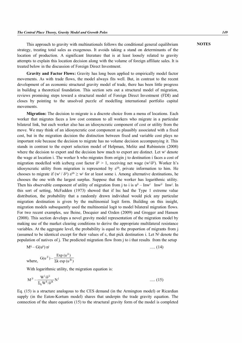
NOTES


This approach to gravity with multinationals follows the conditional general equilibriumstrategy, treating total sales as exogenous. It avoids taking a stand on determinants of thelocation of production. A significant literature that is at least loosely related to gravityattempts to explain this location decision along with the volume of foreign affiliate sales. It istreated below in the discussion of Foreign Direct Investment.

Gravity and Factor Flows: Gravity has long been applied to empirically model factormovements. As with trade flows, the model always fits well. But, in contrast to the recentdevelopment of an economic structural gravity model of trade, there has been little progressin building a theoretical foundation. This section sets out a structural model of migration,reviews promising steps toward a structural model of Foreign Direct Investment (FDI) andcloses by pointing to the unsolved puzzle of modelling international portfolio capitalmovements.

Migration: The decision to migrate is a discrete choice from a menu of locations. Eachworker that migrates faces a low cost common to all workers who migrate in a particularbilateral link, but each worker also has an idiosyncratic component of cost or utility from themove. We may think of an idiosyncratic cost component as plausibly associated with a fixedcost, but in the migration decision the distinction between fixed and variable cost plays noimportant role because the decision to migrate has no volume decision accompanying it. Thisstands in contrast to the export selection model of Helpman, Melitz and Rubinstein (2008)where the decision to export and the decision how much to export are distinct. Let wi denotethe wage at location i. The worker h who migrates from origin j to destination i faces a cost ofmigration modelled with iceberg cost factor ji > 1, receiving net wage (wi/ ji). Worker h’sidiosyncratic utility from migration is represented by jih, private information to him. Hechooses to migrate if (wi / ji) jih wj for at least some i. Among alternative destinations, hechooses the one with the largest surplus. Suppose that the worker has logarithmic utility.Then his observable component of utility of migration from j to i is uji – Inwi Inwji Inwj. Inthis sort of setting, McFadden (1973) showed that if ln had the Type 1 extreme valuedistribution, the probability that a randomly drawn individual would pick any particularmigration destination is given by the multinomial logit form. Building on this insight,migration models subsequently used the multinomial logit to model bilateral migration flows.For two recent examples, see Beine, Docquier and Ozden (2009) and Grogger and Hanson(2008). This section develops a novel gravity model representation of the migration model bymaking use of the market clearing conditions to derive the appropriate multilateral resistancevariables. At the aggregate level, the probability is equal to the proportion of migrants from j(assumed to be identical except for their values of , that pick destination i. Let Nj denote thepopulation of natives of j. The predicted migration flow from j to i that results from the setup

Mij – G(uji) nj ..... (14)

where, )(u exp )(u Exp

– )G(u jk

jiji

With logarithmic utility, the migration equation is:

jjkk

k

jiiji N

/W /W – M ..... (15)

Eq. (15) is a structure analogous to the CES demand (in the Armington model) or Ricardiansupply (in the Eaton-Kortum model) shares that underpin the trade gravity equation. Theconnection of the share equation (15) to the structural gravity form of the model is completed

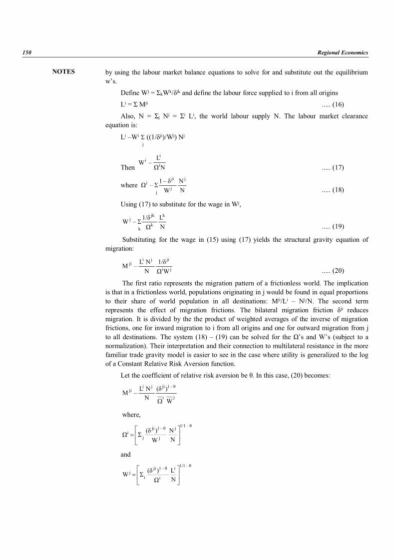
NOTES


by using the labour market balance equations to solve for and substitute out the equilibriumw’s.

Define Wj = kWk/ jk and define the labour force supplied to i from all origins

Li = Mji ..... (16)

Also, N = j Nj = i Li, the world labour supply N. The labour market clearanceequation is:

Li –Wi

j((1/ ji)/Wj) Nj

Then N L

– W i

ii

..... (17)

whereNN

W – 1 –

j

j

ji

j

i

..... (18)

Using (17) to substitute for the wage in Wj,

NL 1/ – W

k

k

jk

k

j

..... (19)

Substituting for the wage in (15) using (17) yields the structural gravity equation ofmigration:

ji

jijiji

W1/

N N L – M

..... (20)

The first ratio represents the migration pattern of a frictionless world. The implicationis that in a frictionless world, populations originating in j would be found in equal proportionsto their share of world population in all destinations: Mji/Li – Nj/N. The second termrepresents the effect of migration frictions. The bilateral migration friction ji reducesmigration. It is divided by the the product of weighted averages of the inverse of migrationfrictions, one for inward migration to i from all origins and one for outward migration from jto all destinations. The system (18) – (19) can be solved for the ’s and W’s (subject to anormalization). Their interpretation and their connection to multilateral resistance in the morefamiliar trade gravity model is easier to see in the case where utility is generalized to the logof a Constant Relative Risk Aversion function.

Let the coefficient of relative risk aversion be . In this case, (20) becomes:

ji

– 1jijiji

W

)(N

N L – M

where,– 1/1j

j

– 1ji j

i

NN

W)(

and– 1/1i

i

– 1ji i

j

NL )( W

NOTES


Here, i and Wj are CES price indexes of migration frictions, one for inward ( i) andone for outward (Wj) migration frictions. These equations are exactly analogous to Andersonand van Wincoop’s gravity, inward( i) and outward (Wj) multilateral resistance equations fortrade, but applied to migration. As with the trade gravity model, outward multilateralresistance gives the sellers’ incidence of the migration costs on average while the inwardmultilateral resistance gives the ‘buyers’ incidence of migration costs. (18)-(20) results fromthe special case = 2.

and W are general equilibrium concepts as is clear because their solution in thesimultaneous systems above involves every bilateral migration cost in the world. They areconditional general equilibrium concepts because the L’s are endogenous in a full generalequilibrium. It is possible in a Ricardian production setting to combined the migration systemwith the trade gravity model to derive equilibrium labour supplies that are functions of theincidence of both migration frictions and trade frictions.

As with trade gravity models, ’s and W’s can be computed once the ’s areeconometrically constructed and the labour supplies Li and population stocks Nj are observed.A normalization is needed.

A similar model has been applied to services trade by Head, Mayer and Ries (2009).Instead of actually changing locations, the foreign worker does the job in his home location.The cost of migration becomes the cost of monitoring the distant worker. Workerproductivities in each location have the Frechet distribution, as in the Eaton-Kortum model.The firm selects workers so as to minimize the log of the delivered unit labour cost. Then thedistribution of log productivities takes the Gumbel form. The fraction of service jobs in origini going to workers in location j has the multinomial logit form. The total numbers of workersand of jobs in each location enter the model in the same way as in the migration model. Isuspect that the choice between off-shoring the service job and migrating the worker can befruitfully addressed with some combination of the two models.

The preceding treatment applies to a stationary equilibrium where the L’s are the resultof M’s fully adjusting labour supplied at each location to its equilibrium value given theinitial stocks of labour (Nj) and the set of migration frictions, the ’s. In adapting the model tofit actual data, the N’s, L’s and M’s are observed at points in time, and with panel data theobservations are linked over time.

If the sequence of observations is regarded as reaching the static equilibrium eachperiod, the observed migration is just that amount needed to reach the equilibrium in eachperiod. This model would be consistent with naive expectations about future wages, or with apure guest worker model in which migration is determined by contemporaneous variablesonly.

So in principle, under this interpretation, the preceding model could be applied at eachdate, all variables now having a time subscript. The alternative is a dynamic model in whichthe migrants form expectations about the sequence of future wages based on underlyingexpectations about the future evolution of the distribution of trade frictions, the populations,and, as we will see following the development of the integrated trade and migration model,variables that predict the demand for labour at all locations. This sophistication requires a bigincrease in complexity, with dubious applicability of rational expectations to unskilledworkers. The other issue raised by thinking of dynamics is the issue of partial adjustment-migration in any one year may not suffice to reach the static equilibrium of the preceding

NOTES


section. In this case, the standard ad hoc approach of partial adjustment due to quadraticadjustment costs might be applied without too large an increase in complexity.

Foreign Direct Investment: Foreign direct investment has been successfully explainedby gravity structures without a theoretical foundation. More recent work has made progresson foundations. Satisfactory foundations are more difficult to find for at least two reasons.First, the location of production question must be answered in an upper level generalequilibrium model, which requires taking a stand on one of many possible production,preference and market structures restricted so as to produce tractable results. Second, thedeterminants of location depend on whether the good in question is vertically or horizontallylinked to other sources of firm profits.

A key element in explaining the location of horizontally linked production is theproximity concentration trade-off: a firm with fixed cost reduces per unit production cost byconcentrating production at one location but can save distribution costs by allocatingproduction in proximity to markets. Even under strong restrictions, the models obtained so farare non-linear and require approximation to be taken to data. Helpman, Melitz and Yeaple(2004) model interaction between horizontally linked exports and foreign affiliate sales,where the firm chooses between exporting from home or investing abroad and selling from aforeign plant. They are able to draw inferences from aggregate data by modellingheterogeneous productivity of firms with a Pareto distribution. Fixed costs of export and ofinvesting abroad serve to select firms into non-traders, exporters and multinationals withratios that vary market by market due to trade costs modeled as transport costs and tariffsonly, omitting the usual gravity variables. Their empirical application with US data obtainsfairly good results in explaining the ratio of exports to foreign affiliate sales with a linearapproximation to their underlying non-linear model. The model fits much less well thanstandard export gravity equations, not surprising because the dependent variable is differentand the question addressed is more difficult to answer. Kleinert and Toubal (2010) extendHelpman, Melitz and Yeaple to allow for fixed setup costs that rise with distance, a wrinklethat can explain why foreign affiliate sales can fall rather than rise with distance as the earlierproximity-concentration trade-off suggested. They also derive a gravity-type relationshipfrom two other structures, a vertical integration model and a two country factor proportionsmodel of fragmentation.

Bergstrand and Egger (2007) offer a gravity model of FDI derived from the knowledgebased capital theory of horizontal multi-national enterprises. Their objective is a full generalequilibrium model that can explain trade, foreign affiliate sales and foreign direct investment.They simulate a theoretical model that generates non-linear relationships between exports,affiliate sales and their exogenous determinants. Then they fit an approximate empiricalrelationship to the generated data and take the same relationship to actual data, with somesuccess. A limitation of their model is that, though the factor proportions model with threefactors is used to explain simultaneous exports and affiliate sales, the countries in theirsimulation setup have identical endowment proportions and differ only in size.

Keller and Yeaple (2009) develop a gravity model of vertically integrated intra-firmtrade featuring trade costs with two elements, a standard iceberg trade cost and acommunication cost that rises with the complexity of the firm’s technology. Input complexityraises technology transfer costs while the costs of embodied technology transfer areindependent of complexity and increasing in trade costs. An increase in trade costs reducesforeign affiliate sales and this effect is strongest in the most complex sectors. In contrast, anincrease in trade costs reduces the imports of foreign affiliates and this effect is weakest in

NOTES


the most complex sectors. Like the standard trade gravity model, Keller and Yeaple’s modelof foreign affiliate sales permits inference about trade costs from observable trade flows.

Keller and Yeaple report fairly good results estimating the model using confidential dataon US multinational firm activity from the Bureau of Economic Analysis. The role played bycommunication cost interacting with technological complexity, thus, appears likely to behelpful in explaining the rising share (in total trade) of intra-firm trade and also the risingshare of trade in intermediates.

An alternative strategy along the lines of the conditional general equilibrium approachoutlined above for migration appears useful. The migration decision model could apply toFDI since the location decision for a plant is similar to the location decision of a migrant.(Unlike migration but like trade, FDI involves a volume decision along with a participationdecision.) The rate of return on investment could be taken as exogenous in a conditionalgeneral equilibrium approach just as wages are taken as exogenous in the migration gravitymodel, while market clearing conditions apply just as in the migration model. Idiosyncraticcost factors would apply to the various investment projects, just as they do to the individualmigrants. The Keller-Yeaple model of vertically integrated intra-firm trade offers a structurefor identifying one type of cost. A weakness in the extension by analogy is in riskdiversification. Migrants cannot diversify their risks, but firms can, though with limitedpossibilities that may be very limited for FDI. The potential risk diversification would modifythe utility derived from each location choice. The discrete choice approach faces trulyformidable modelling challenges in endogenizing the investment rates of return, unlike thewage equation suggested by the migration model.

A promising start on these lines is by Head and Ries (2008). Potential acquisitions go tothe highest bidder, who bids based on his anticipated return net of monitoring costs that risewith distance and other standard gravity variables. The probability of the winning bid goingto source country i takes the multinomial logit form. The mass variables are the stocks ofprojects in each host country and each source country’s share of world bidders.

Portfolio Investment: Martin and Rey (2004) offer the first gravity type model ofinternational portfolio investment. The coefficient of relative risk aversion plays the role, inequilibrium, of the elasticity of substitution in the CES demand specification. Whileappealing as a rationale for the gravity application of Portes and Rey (2005), the Martin andRey model does not provide a fully satisfactory foundation for gravity models of investmentflows because: (i) trade is assumed to be frictionless, (ii) investment costs are uniform, and(iii) most important, the analysis is restricted to two countries. The third party effects thatplay a big role in the gravity model of trade (and of migration) cannot be treated.

Integrated Superstructure: The gravity model nests inside a general equilibriumsuperstructure. As pointed out in Anderson and van Wincoop (2004), modularity implies thatthe problem of resource and expenditure allocation across sectors in the general equilibriumsuperstructure can be treated separably from the gravity module problem of distributionwithin sectors to destinations or from origins. Consistency between the two levels of theproblem requires fixed point calculations in general, but the economy of thought andcomputation due to separability is extremely useful, and in particular makes it possible tointegrate gravity with a wide class of general equilibrium production models. So far, onlyvery simple production models have been used for full general equilibrium comparativestatics, but I anticipate that this situation will change.

NOTES


The simplest production structure is an endowments economy. Anderson and vanWincoop (2003) use the endowments model to calculate the effect of eradicating theUS-Canada border on their estimated gravity model of trade between US states, Canadianprovinces and the aggregated rest of the world.

Another attractive candidate is the Ricardian production model. Eaton and Kortum(2002) nest gravity inside a Ricardian model of production, a choice followed by a host ofsubsequent researchers such as Arkolakis (2008). An important feature of these models is theaction on the extensive margin, as industries arise or disappear. In the Eaton-Kortum modelof 2002, the extensive margin is the only margin. Arkolakis and others have variants in whichboth extensive and intensive margins are active. This is an important feature becausedisaggregated trade data and especially firm level data indicate that both margins are active.

Between the two extremes of zero and infinite elasticity of transformation of theendowments and Ricardian models lie a host of more complex production structures in whichaction occurs on the intensive margin of production when relative prices change, leading toanother channel of interaction between the gravity modules in each sector (and resultingbuyers’ and sellers’ incidences) and the pattern of production. Consistency between themodules is achieved by using (9) to normalize the ’s in each sector. I think the future willsee work with these more complex general equilibrium features.

Migration of labour and capital in the form of FDI has been given a complete gravityrepresentation in this essay. In the integrated superstructure, it can be treated simultaneouslywith the trade modules. In this setting, multilateral resistance in trade has significant effectson migration and vice versa. I anticipate that development of this link will be useful.

A number of authors have constructed integrated models that motivate econometricwork aimed at discriminating between one or another specification of the upper levelproduction and market structure. A summary of work on these lines is in Feenstra (2004),Chapter 5, where the main focus is on the link between gravity and increasing returns to scale.Research has continued on these lines, but I will not review it here.

So, the gravity model is a poor vehicle for inferences about returns to scale, marketstructure and the global general equilibrium links between economies. Under suchcircumstances, gravity is about the distribution of given amounts of goods in each origindrawn by given amounts of expenditure in each destination, enabling inference about tradecosts from the deviation of observed distribution from the frictionless equilibrium. Thedeterminants of total shipments and total expenditures are irrelevant to this inference becausecountry fixed effects are a consistent control that does not require taking a stand on anyparticular production or market structure model. Conversely, the cross-section variation ofbilateral trade does not seem likely to have much useful information about the determinationof national total shipments or expenditure. Interdependence is so deeply wound between thesevariables in the full general equilibrium model that inference about structure seemsimplausible. In contrast, simulation models look reasonably promising as a source of insight.

This idiosyncratic review of work on the gravity model suggests that the story is notover, so a conclusion can only point to potential future chapters. Distribution broadly definedconsumes a very large share of the world’s resources and gravity has proven to be the mostgenerally useful empirical model for understanding the distribution of goods and factors ofproduction. It appears to work well at almost any scale. The progress in structural modellingof gravity has yielded three distinct rationales for the same observationally equivalent modelof the distribution of economic flows between origins and destinations, one based on the

NOTES


demand side (the CES/Armington model), one based on the supply side (the Eaton-Kortummodel), and one based on a discrete choice model of the individual actor transferring thegoods or factors. Further work may suggest ways to discriminate between these. Thestructural modelling of gravity imposes trade separability, permitting gravity modules to benested inside a wide range of general equilibrium superstructures. Future work withsimulation models may suggest which of many candidate general equilibrium productionmodels do better.

The problem of zeroes in the trade and factor flows data has been addressed with somesuccess, particularly by Helpman, Melitz and Rubinstein. But I expect future work to dobetter. The CES framework (with elasticity of substitution greater than one) is unsuitable fordescribing small amounts of trade. The translog cost function, in particular, seems likely toyield better descriptions and better understanding of why so many potential flows are equal tozero. This is so even if, as in HMR, fixed export costs play an important role in selectingfirms to export. Incidence measures produced by Anderson and Yotov have been featured inthis review. If the profession agrees that they are as interesting and useful as they appear tome, more work is needed to see how believable the measures are. As it stands, they arecompletely reliant on CES structure. How well does the CES do in representing the worldeconomy? This is an especially important question in light of the zeroes question in thepreceding paragraph.

4.4 GROWTH POLES

Growth-pole Strategies in Regional Economic Planning: A RetrospectiveView, Origins and Advocacy

One of the more intriguing aspects of the analysis and practice of regional economicplanning over the past several decades has been the changing attitude towards the growth-pole strategy. This strategy or family of strategies has been proposed in a variety of settings,and is therefore not easily generalized. Certain common features can be identified, however.The growth-pole strategy typically involves the focusing of investment at a limited number oflocations (usually as part of a deliberate effort to modify regional spatial structure), in anattempt to encourage economic activity and thereby raise levels of welfare within a region.By the mid-1960s, the growth-pole strategy had emerged as the object of considerablefascination and enthusiasm, and was viewed as an idea in good currency, to use the borrowedphrase of Lasue An. Indeed, a newcomer to the field at that time could have been excused forthinking that no matter what the nature of the regional problem, it would be most effectivelyovercome by the adoption of a growth-pole strategy. Doubters subsequently emerged,including Gilbert (1974) and Moseley (1973), but they were few in number and theirwarnings went largely unheeded; such was the spirit of the times. Large areas within the fieldof regional terms of the growth-pole strategy. Commenting later on this trend, Kuklinski(1978, tellingly observed: Sometimes the judgement is expressed that growth-pole theory isthe closest approximation to the general theory of regional development.

The period from the mid-1960s to the mid-1970s saw a rapid expansion of academicinterest in growth-pole strategies, with numerous conference sessions, collected volumes andjournal articles devoted to the subject. Coinciding with this, and probably not unrelated to it,were the many attempts to apply the strategy in a variety of settings within developing as wellas developed economies, the nations of Latin America being among the early adopters. In thelight of subsequent experience, however, the strategy can only be judged to have been

NOTES


unsuccessful, at least in the sense that it failed to achieve the primary objectives of policywithin the time-interval envisaged. There were, it is true, cases where it was broadlysuccessful, either by design or good fortune, and other cases where certain facets of thestrategy achieved a measure of success. Nevertheless, the instances where the strategy wasimplemented in a consistent manner and carried through to fruition are few in number. In fact,the recent history of regional economic planning in many parts of the world is littered withexamples of growth-pole strategies having failed or having been prematurely abandoned. It ishardly surprising therefore that present-day attitudes towards growth-pole strategies stand inmarked contrast to those of the 1960s. Despite spirited and cogently argued defences of thegrowth-pole strategy during the intervening years (Boisier, 1980; Hansen, 1975; Richardson,1978), it has fallen from favour. Governments have largely turned their backs on it(Breathnach, 1982; Conroy, 1973), and among planners it tends to be regarded as passe or assome relic of earlier planning practice. Frequently, it is rejected out of hand, and some eventake the view that the strategy represents a fundamentally inappropriate approach to regionaleconomic problems. Gore (1984) and Lipton (1977), for instance, come very close to thisposition. Among others, the notion of a growth-pole strategy has aroused a suspicion, if nothostility, on ideological grounds (Coraggio, 1973). Such a volte face within the field ofregional economic planning over an interval of not much more than three decades isdisquieting. It suggests at the very least a superspeciality of approach and more seriouslyperhaps an inability or an unwillingness to subject new concepts to close scrutiny.

Enough time has probably elapsed for the chequered career of the growth-pole strategyto be placed into perspective. If it were simply a case of a particular planning strategy havingshown itself to be ineffective, then the episode could simply be written up in the annals ofplanning history in the usual manner. Useful as such an account might be, the examination ofgrowth-pole strategy should extend beyond the purely historical, if only because the reasonssurrounding its frequent failure go to the very heart of regional economic planning, and havepowerful implications for virtually every form of policy intervention at the regional scale. Inother words, the kinds of questions that needed to be asked of growth-pole strategy (but, aswe shall see, were not) are the very questions that should be asked of any other strategy oremphasis in regional economic planning. The analysis of growth-pole strategy thus has arelevance and generality which extend far beyond the strategy itself. As will be apparent, thearguments to follow represent neither a dismissal of growth-pole strategy nor an attempt torehabilitate it. Rather, the concern is with drawing attention to its complex and highlyconditional nature. What will also become evident is the absence of an adequate frameworkor general theory of regional economic policy, within which the growth-pole strategy couldhave been evaluated, either conceptually or operationally. In fact, the absence of such aframework goes a long way to explaining not only the initial enthusiasm towards the growth-pole strategy, but also the more recent rejection of it. There were also a number of confusionsthat have bedevilled the conceptualization of growth-pole strategy from the very beginningand attention now turns to certain of these.

Some Underlying ConfusionsMuch of the early writing on growth-pole strategies failed to make a clear distinction

between the growth pole as a feature of a dynamic space economy and the growth pole as akey element in a strategy designed to improve the performance of a regional economicsystem, i.e., a distinct ion between the natural or spontaneous’ growth pole and the ‘planned’or ‘induced’ growth pole. The concept of the natural growth pole derives directly from thework of Perroux (1955), who viewed growth within an economy as stemming from the

NOTES


effects of disequilibrium and domination, and necessarily occurring unevenly. To quote awell-known passage from Perroux (1955) in this connection — Growth does not appeareverywhere at the same time; it appears at points or poles of growth with varying intensity; itspreads along various channels and with differing overall effects on the whole economy. To alarge extent, Perroux couched his argument in terms of abstract economic space, a conceptthat he had developed earlier (Perroux, 1950). Within such a space, polarization wasmeasured with respect to the intensity of inter-industry transactions. Nevertheless, Perrouxfully recognized the possibility that a growth pole in economic space might also exist as aterritorial entity and considered the implications of this. Thus, he drew attention to thereinforcing influences of spatial concentration, the effects on inter-regional disparities and theimpact of the growth pole on its environment; such an emphasis was also present in hisearlier work on the Ruhr district of Germany as well as in his later contributions.

The concept of the growth pole in geographical space was subsequently developed byHansen (1967) and Hermansen (1972), following the lead of various Francophone economists,most notably Paelinck (1965, 1968), Aydalot (1965) and Boudeville (1966). But this was notalways undertaken satisfactorily. For example, one definition of a growth pole ingeographical space, in many respects typical of the period, involved a set of expandingindustries located in an urban area and inducing further development of economic activitythroughout its zone of influence.

Such a definition immediately raises the following questions: If an urban centre withexpanding industries does not induce favourable effects throughout its zone of influence (acommon occurrence), does this imply that it cannot be regarded as a growth pole? And canthe growth poles of London, New York and Paris in the 19th century, or Atlanta, Lyon andMunich in the 20th century, be satisfactorily defined in these terms?

Definitions of this kind reflected a tendency at the time to treat the growth pole ingeographical space as an urban centre which possessed the attributes of the growth pole inabstract economic space. However, this represents an unjustified and analytically unhelpfulrestriction, which robs the concept of much of its usefulness in regional economic analysis. Infact, a case can be made for viewing the growth pole in geographical space as any urbancentre (above some minimum threshold) which displays specified growth characteristics (inabsolute and relative terms), with no presumption about the bases of growth or about theeffects on its zone of influence (Parr, 1973). Contrary to the opinion of a number of writers,there is no unambiguous correspondence between abstract economic space and geographicalspace. Reality is such that a given structure (a given level of polarization) in economic spacecan translate into a variety of structures in geographical space, and vice versa. The growthpole in geographical space is an entity in its own right, which may have differingmanifestations in economic space and needs to be analyzed accordingly.

By the early 1960s, this notion of the growth pole in geographical space began toassume a normative aspect. Attention was given to the possibility of pursuing a growth-polestrategy, the cornerstone of which would be the activation of planned or induced growth poles.Two rather different strands of thinking lay behind this. First, it had been recognized for sometime that development in a regional or national economy was associated in a causal sensewith a tendency towards concentration and polarization, and the historical evidence for thiswas abundant. It, therefore, followed that the deliberate focusing of investment at a limitednumber of centres would satisfy a necessary condition for development.

Such arguments recognized the important fact that development was not independent ofthe nature of the spatial structure of the economy and that in many regional economies an

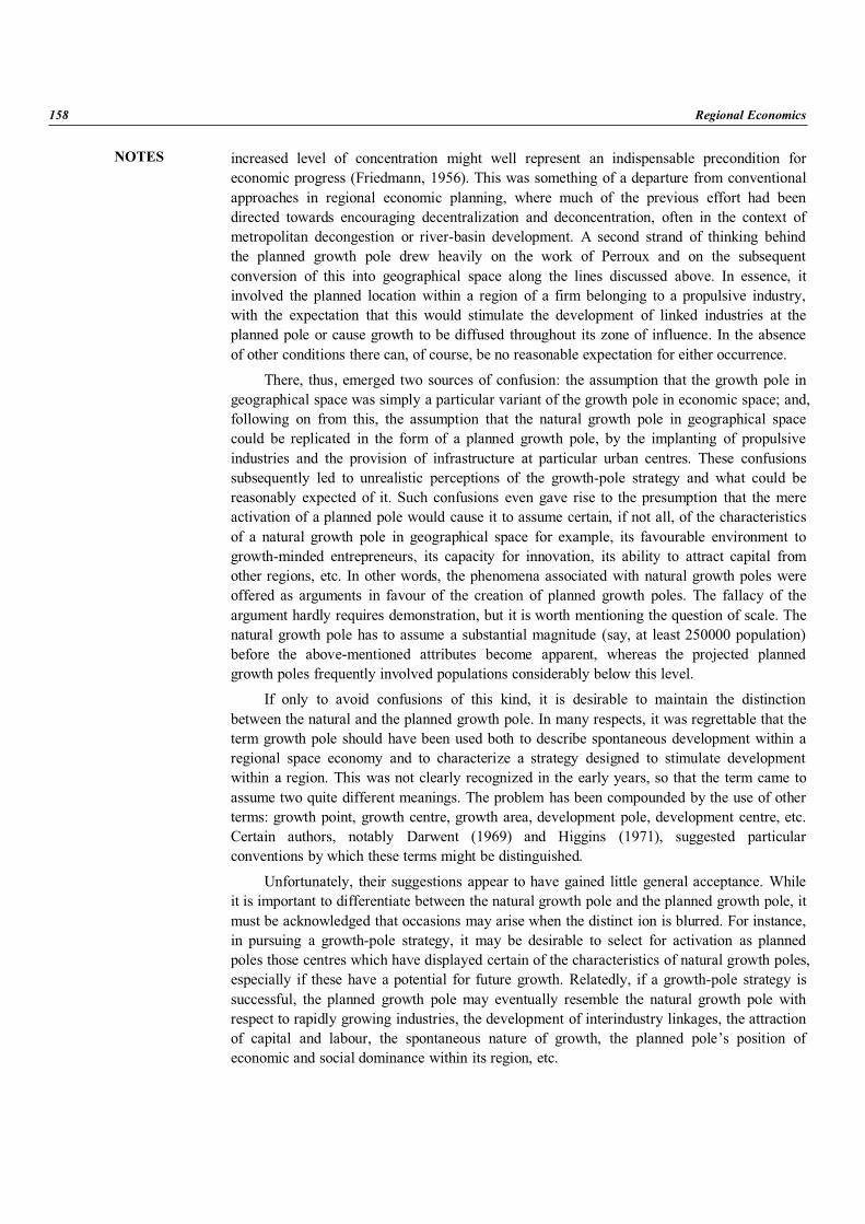
NOTES


increased level of concentration might well represent an indispensable precondition foreconomic progress (Friedmann, 1956). This was something of a departure from conventionalapproaches in regional economic planning, where much of the previous effort had beendirected towards encouraging decentralization and deconcentration, often in the context ofmetropolitan decongestion or river-basin development. A second strand of thinking behindthe planned growth pole drew heavily on the work of Perroux and on the subsequentconversion of this into geographical space along the lines discussed above. In essence, itinvolved the planned location within a region of a firm belonging to a propulsive industry,with the expectation that this would stimulate the development of linked industries at theplanned pole or cause growth to be diffused throughout its zone of influence. In the absenceof other conditions there can, of course, be no reasonable expectation for either occurrence.

There, thus, emerged two sources of confusion: the assumption that the growth pole ingeographical space was simply a particular variant of the growth pole in economic space; and,following on from this, the assumption that the natural growth pole in geographical spacecould be replicated in the form of a planned growth pole, by the implanting of propulsiveindustries and the provision of infrastructure at particular urban centres. These confusionssubsequently led to unrealistic perceptions of the growth-pole strategy and what could bereasonably expected of it. Such confusions even gave rise to the presumption that the mereactivation of a planned pole would cause it to assume certain, if not all, of the characteristicsof a natural growth pole in geographical space for example, its favourable environment togrowth-minded entrepreneurs, its capacity for innovation, its ability to attract capital fromother regions, etc. In other words, the phenomena associated with natural growth poles wereoffered as arguments in favour of the creation of planned growth poles. The fallacy of theargument hardly requires demonstration, but it is worth mentioning the question of scale. Thenatural growth pole has to assume a substantial magnitude (say, at least 250000 population)before the above-mentioned attributes become apparent, whereas the projected plannedgrowth poles frequently involved populations considerably below this level.

If only to avoid confusions of this kind, it is desirable to maintain the distinctionbetween the natural and the planned growth pole. In many respects, it was regrettable that theterm growth pole should have been used both to describe spontaneous development within aregional space economy and to characterize a strategy designed to stimulate developmentwithin a region. This was not clearly recognized in the early years, so that the term came toassume two quite different meanings. The problem has been compounded by the use of otherterms: growth point, growth centre, growth area, development pole, development centre, etc.Certain authors, notably Darwent (1969) and Higgins (1971), suggested particularconventions by which these terms might be distinguished.

Unfortunately, their suggestions appear to have gained little general acceptance. Whileit is important to differentiate between the natural growth pole and the planned growth pole, itmust be acknowledged that occasions may arise when the distinct ion is blurred. For instance,in pursuing a growth-pole strategy, it may be desirable to select for activation as plannedpoles those centres which have displayed certain of the characteristics of natural growth poles,especially if these have a potential for future growth. Relatedly, if a growth-pole strategy issuccessful, the planned growth pole may eventually resemble the natural growth pole withrespect to rapidly growing industries, the development of interindustry linkages, the attractionof capital and labour, the spontaneous nature of growth, the planned pole’s position ofeconomic and social dominance within its region, etc.

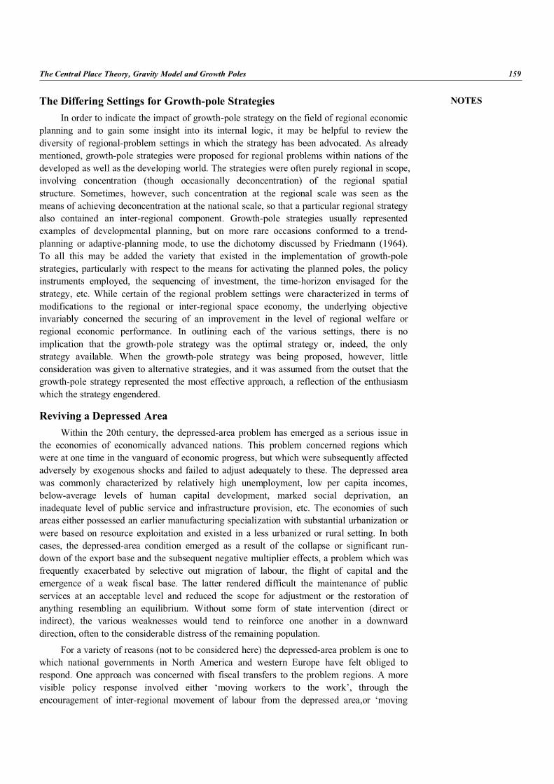
NOTES


The Differing Settings for Growth-pole StrategiesIn order to indicate the impact of growth-pole strategy on the field of regional economic

planning and to gain some insight into its internal logic, it may be helpful to review thediversity of regional-problem settings in which the strategy has been advocated. As alreadymentioned, growth-pole strategies were proposed for regional problems within nations of thedeveloped as well as the developing world. The strategies were often purely regional in scope,involving concentration (though occasionally deconcentration) of the regional spatialstructure. Sometimes, however, such concentration at the regional scale was seen as themeans of achieving deconcentration at the national scale, so that a particular regional strategyalso contained an inter-regional component. Growth-pole strategies usually representedexamples of developmental planning, but on more rare occasions conformed to a trend-planning or adaptive-planning mode, to use the dichotomy discussed by Friedmann (1964).To all this may be added the variety that existed in the implementation of growth-polestrategies, particularly with respect to the means for activating the planned poles, the policyinstruments employed, the sequencing of investment, the time-horizon envisaged for thestrategy, etc. While certain of the regional problem settings were characterized in terms ofmodifications to the regional or inter-regional space economy, the underlying objectiveinvariably concerned the securing of an improvement in the level of regional welfare orregional economic performance. In outlining each of the various settings, there is noimplication that the growth-pole strategy was the optimal strategy or, indeed, the onlystrategy available. When the growth-pole strategy was being proposed, however, littleconsideration was given to alternative strategies, and it was assumed from the outset that thegrowth-pole strategy represented the most effective approach, a reflection of the enthusiasmwhich the strategy engendered.

Reviving a Depressed AreaWithin the 20th century, the depressed-area problem has emerged as a serious issue in

the economies of economically advanced nations. This problem concerned regions whichwere at one time in the vanguard of economic progress, but which were subsequently affectedadversely by exogenous shocks and failed to adjust adequately to these. The depressed areawas commonly characterized by relatively high unemployment, low per capita incomes,below-average levels of human capital development, marked social deprivation, aninadequate level of public service and infrastructure provision, etc. The economies of suchareas either possessed an earlier manufacturing specialization with substantial urbanization orwere based on resource exploitation and existed in a less urbanized or rural setting. In bothcases, the depressed-area condition emerged as a result of the collapse or significant run-down of the export base and the subsequent negative multiplier effects, a problem which wasfrequently exacerbated by selective out migration of labour, the flight of capital and theemergence of a weak fiscal base. The latter rendered difficult the maintenance of publicservices at an acceptable level and reduced the scope for adjustment or the restoration ofanything resembling an equilibrium. Without some form of state intervention (direct orindirect), the various weaknesses would tend to reinforce one another in a downwarddirection, often to the considerable distress of the remaining population.

For a variety of reasons (not to be considered here) the depressed-area problem is one towhich national governments in North America and western Europe have felt obliged torespond. One approach was concerned with fiscal transfers to the problem regions. A morevisible policy response involved either ‘moving workers to the work’, through theencouragement of inter-regional movement of labour from the depressed area,or ‘moving

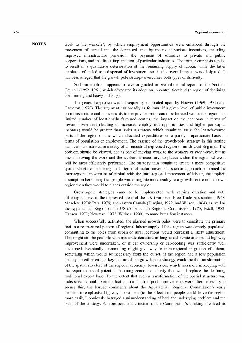
NOTES


work to the workers’, by which employment opportunities were enhanced through themovement of capital into the depressed area by means of various incentives, includingimproved infrastructure provision, the payment of subsidies to private and publiccorporations, and the direct implantation of particular industries. The former emphasis tendedto result in a qualitative deterioration of the remaining supply of labour, while the latteremphasis often led to a dispersal of investment, so that its overall impact was dissipated. Ithas been alleged that the growth-pole strategy overcomes both types of difficulty.

Such an emphasis appears to have originated in two influential reports of the ScottishCouncil (1952, 1961) which advocated its adoption in central Scotland (a region of decliningcoal mining and heavy industry).

The general approach was subsequently elaborated upon by Hoover (1969, 1971) andCameron (1970). The argument ran broadly as follows: if a given level of public investmenton infrastructure and inducements to the private sector could be focused within the region at alimited number of locationally favoured centres, the impact on the economy in terms ofinward investment (leading to increased employment opportunities and higher per capitaincomes) would be greater than under a strategy which sought to assist the least-favouredparts of the region or one which allocated expenditures on a purely proportionate basis interms of population or employment. The essence of the growth-pole strategy in this settinghas been summarized in a study of an industrial depressed region of north-west England: Theproblem should be viewed, not as one of moving work to the workers or vice versa, but asone of moving the work and the workers if necessary, to places within the region where itwill be most efficiently performed. The strategy thus sought to create a more competitivespatial structure for the region. In terms of factor movement, such an approach combined theinter-regional movement of capital with the intra-regional movement of labour, the implicitassumption here being that people would migrate more readily to a growth centre in their ownregion than they would to places outside the region.

Growth-pole strategies came to be implemented with varying duration and withdiffering success in the depressed areas of the UK (European Free Trade Association, 1968;Moseley, 1974; Parr, 1979) and eastern Canada (Higgins, 1972; and Wilson, 1964), as well asthe Appalachian Region of the US (Appalachian Regional Commission, 1970; Estall, 1982;Hansen, 1972; Newman, 1972; Widner, 1990), to name but a few instances.

When successfully activated, the planned growth poles were to constitute the primaryfoci in a restructured pattern of regional labour supply. If the region was densely populated,commuting to the poles from urban or rural locations would represent a likely adjustment.This might still be possible with moderate densities, as long as deliberate attempts at highwayimprovement were undertaken, or if car ownership or car-pooling was sufficiently welldeveloped. Eventually, commuting might give way to intra-regional migration of labour,something which would be necessary from the outset, if the region had a low populationdensity. In either case, a key feature of the growth-pole strategy would be the transformationof the spatial structure of the regional economy, towards one which was more in keeping withthe requirements of potential incoming economic activity that would replace the decliningtraditional export base. To the extent that such a transformation of the spatial structure wasindispensable, and given the fact that radical transport improvements were often necessary tosecure this, the barbed comments about the Appalachian Regional Commission’s earlydecision to emphasise highway investment (to the effect that ‘people could leave the regionmore easily’) obviously betrayed a misunderstanding of both the underlying problem and thebasis of the strategy. A more pertinent criticism of the Commission’s thinking involved its

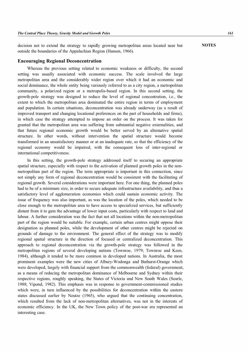
NOTES


decision not to extend the strategy to rapidly growing metropolitan areas located near butoutside the boundaries of the Appalachian Region (Hansen, 1966).

Encouraging Regional DeconcentrationWhereas the previous setting related to economic weakness or difficulty, the second

setting was usually associated with economic success. The scale involved the largemetropolitan area and the considerably wider region over which it had an economic andsocial dominance, the whole entity being variously referred to as a city region, a metropolitancommunity, a polarized region or a metropolis-based region. In this second setting, thegrowth-pole strategy was designed to reduce the level of regional concentration, i.e., theextent to which the metropolitan area dominated the entire region in terms of employmentand population. In certain situations, deconcentration was already underway (as a result ofimproved transport and changing locational preferences on the part of households and firms),in which case the strategy attempted to impose an order on the process. It was taken forgranted that the metropolitan area was suffering from substantial negative externalities, andthat future regional economic growth would be better served by an alternative spatialstructure. In other words, without intervention the spatial structure would becometransformed in an unsatisfactory manner or at an inadequate rate, so that the efficiency of theregional economy would be impaired, with the consequent loss of inter-regional orinternational competitiveness.

In this setting, the growth-pole strategy addressed itself to securing an appropriatespatial structure, especially with respect to the activation of planned growth poles in the non-metropolitan part of the region. The term appropriate is important in this connection, sincenot simply any form of regional deconcentration would be consistent with the facilitating ofregional growth. Several considerations were important here. For one thing, the planned poleshad to be of a minimum size, in order to secure adequate infrastructure availability, and thus asatisfactory level of agglomeration economies which could sustain economic activity. Theissue of frequency was also important, as was the location of the poles, which needed to beclose enough to the metropolitan area to have access to specialized services, but sufficientlydistant from it to gain the advantage of lower input costs, particularly with respect to land andlabour. A further consideration was the fact that not all locations within the non-metropolitanpart of the region would be suitable. For example, certain urban centres might oppose theirdesignation as planned poles, while the development of other centres might be rejected ongrounds of damage to the environment. The general effect of the strategy was to modifyregional spatial structure in the direction of focused or centralized deconcentration. Thisapproach to regional deconcentration via the growth-pole strategy was followed in themetropolitan regions of several developing nations (Townroe, 1979; Townroe and Keen,1984), although it tended to be more common in developed nations. In Australia, the mostprominent examples were the new cities of Albury-Wodonga and Bathurst-Orange whichwere developed, largely with financial support from the commonwealth (federal) government,as a means of reducing the metropolitan dominance of Melbourne and Sydney within theirrespective regions, roughly speaking, the States of Victoria and New South Wales (Searle,1988; Vipond, 1982). This emphasis was in response to government-commissioned studieswhich were, in turn influenced by the possibilities for deconcentration within the easternstates discussed earlier by Neutze (1965), who argued that the continuing concentration,which resulted from the lack of non-metropolitan alternatives, was not in the interests ofeconomic efficiency. In the UK, the New Town policy of the post-war era represented aninteresting case.

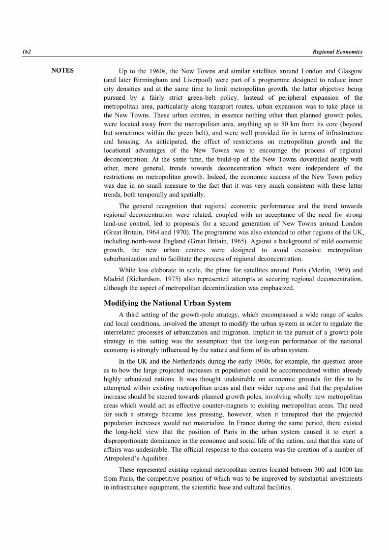
NOTES


Up to the 1960s, the New Towns and similar satellites around London and Glasgow(and later Birmingham and Liverpool) were part of a programme designed to reduce innercity densities and at the same time to limit metropolitan growth, the latter objective beingpursued by a fairly strict green-belt policy. Instead of peripheral expansion of themetropolitan area, particularly along transport routes, urban expansion was to take place inthe New Towns. These urban centres, in essence nothing other than planned growth poles,were located away from the metropolitan area, anything up to 50 km from its core (beyondbut sometimes within the green belt), and were well provided for in terms of infrastructureand housing. As anticipated, the effect of restrictions on metropolitan growth and thelocational advantages of the New Towns was to encourage the process of regionaldeconcentration. At the same time, the build-up of the New Towns dovetailed neatly withother, more general, trends towards deconcentration which were independent of therestrictions on metropolitan growth. Indeed, the economic success of the New Town policywas due in no small measure to the fact that it was very much consistent with these lattertrends, both temporally and spatially.

The general recognition that regional economic performance and the trend towardsregional deconcentration were related, coupled with an acceptance of the need for strongland-use control, led to proposals for a second generation of New Towns around London(Great Britain, 1964 and 1970). The programme was also extended to other regions of the UK,including north-west England (Great Britain, 1965). Against a background of mild economicgrowth, the new urban centres were designed to avoid excessive metropolitansuburbanization and to facilitate the process of regional deconcentration.

While less elaborate in scale, the plans for satellites around Paris (Merlin, 1969) andMadrid (Richardson, 1975) also represented attempts at securing regional deconcentration,although the aspect of metropolitan decentralization was emphasized.

Modifying the National Urban SystemA third setting of the growth-pole strategy, which encompassed a wide range of scales

and local conditions, involved the attempt to modify the urban system in order to regulate theinterrelated processes of urbanization and migration. Implicit in the pursuit of a growth-polestrategy in this setting was the assumption that the long-run performance of the nationaleconomy is strongly influenced by the nature and form of its urban system.

In the UK and the Netherlands during the early 1960s, for example, the question aroseas to how the large projected increases in population could be accommodated within alreadyhighly urbanized nations. It was thought undesirable on economic grounds for this to beattempted within existing metropolitan areas and their wider regions and that the populationincrease should be steered towards planned growth poles, involving wholly new metropolitanareas which would act as effective counter-magnets to existing metropolitan areas. The needfor such a strategy became less pressing, however, when it transpired that the projectedpopulation increases would not materialize. In France during the same period, there existedthe long-held view that the position of Paris in the urban system caused it to exert adisproportionate dominance in the economic and social life of the nation, and that this state ofaffairs was undesirable. The official response to this concern was the creation of a number ofAtropolesd’e Aquilibre.

These represented existing regional metropolitan centres located between 300 and 1000 kmfrom Paris, the competitive position of which was to be improved by substantial investmentsin infrastructure equipment, the scientific base and cultural facilities.

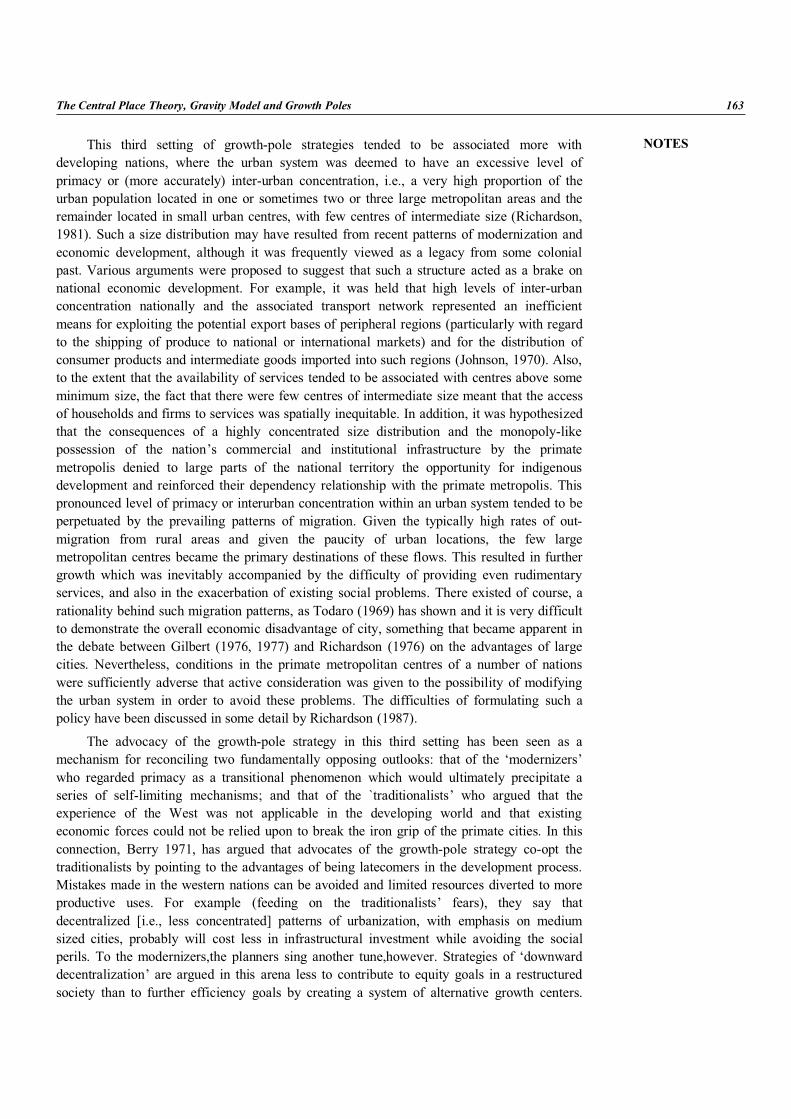
NOTES


This third setting of growth-pole strategies tended to be associated more withdeveloping nations, where the urban system was deemed to have an excessive level ofprimacy or (more accurately) inter-urban concentration, i.e., a very high proportion of theurban population located in one or sometimes two or three large metropolitan areas and theremainder located in small urban centres, with few centres of intermediate size (Richardson,1981). Such a size distribution may have resulted from recent patterns of modernization andeconomic development, although it was frequently viewed as a legacy from some colonialpast. Various arguments were proposed to suggest that such a structure acted as a brake onnational economic development. For example, it was held that high levels of inter-urbanconcentration nationally and the associated transport network represented an inefficientmeans for exploiting the potential export bases of peripheral regions (particularly with regardto the shipping of produce to national or international markets) and for the distribution ofconsumer products and intermediate goods imported into such regions (Johnson, 1970). Also,to the extent that the availability of services tended to be associated with centres above someminimum size, the fact that there were few centres of intermediate size meant that the accessof households and firms to services was spatially inequitable. In addition, it was hypothesizedthat the consequences of a highly concentrated size distribution and the monopoly-likepossession of the nation’s commercial and institutional infrastructure by the primatemetropolis denied to large parts of the national territory the opportunity for indigenousdevelopment and reinforced their dependency relationship with the primate metropolis. Thispronounced level of primacy or interurban concentration within an urban system tended to beperpetuated by the prevailing patterns of migration. Given the typically high rates of out-migration from rural areas and given the paucity of urban locations, the few largemetropolitan centres became the primary destinations of these flows. This resulted in furthergrowth which was inevitably accompanied by the difficulty of providing even rudimentaryservices, and also in the exacerbation of existing social problems. There existed of course, arationality behind such migration patterns, as Todaro (1969) has shown and it is very difficultto demonstrate the overall economic disadvantage of city, something that became apparent inthe debate between Gilbert (1976, 1977) and Richardson (1976) on the advantages of largecities. Nevertheless, conditions in the primate metropolitan centres of a number of nationswere sufficiently adverse that active consideration was given to the possibility of modifyingthe urban system in order to avoid these problems. The difficulties of formulating such apolicy have been discussed in some detail by Richardson (1987).

The advocacy of the growth-pole strategy in this third setting has been seen as amechanism for reconciling two fundamentally opposing outlooks: that of the ‘modernizers’who regarded primacy as a transitional phenomenon which would ultimately precipitate aseries of self-limiting mechanisms; and that of the `traditionalists’ who argued that theexperience of the West was not applicable in the developing world and that existingeconomic forces could not be relied upon to break the iron grip of the primate cities. In thisconnection, Berry 1971, has argued that advocates of the growth-pole strategy co-opt thetraditionalists by pointing to the advantages of being latecomers in the development process.Mistakes made in the western nations can be avoided and limited resources diverted to moreproductive uses. For example (feeding on the traditionalists’ fears), they say thatdecentralized [i.e., less concentrated] patterns of urbanization, with emphasis on mediumsized cities, probably will cost less in infrastructural investment while avoiding the socialperils. To the modernizers,the planners sing another tune,however. Strategies of ‘downwarddecentralization’ are argued in this arena less to contribute to equity goals in a restructuredsociety than to further efficiency goals by creating a system of alternative growth centers.

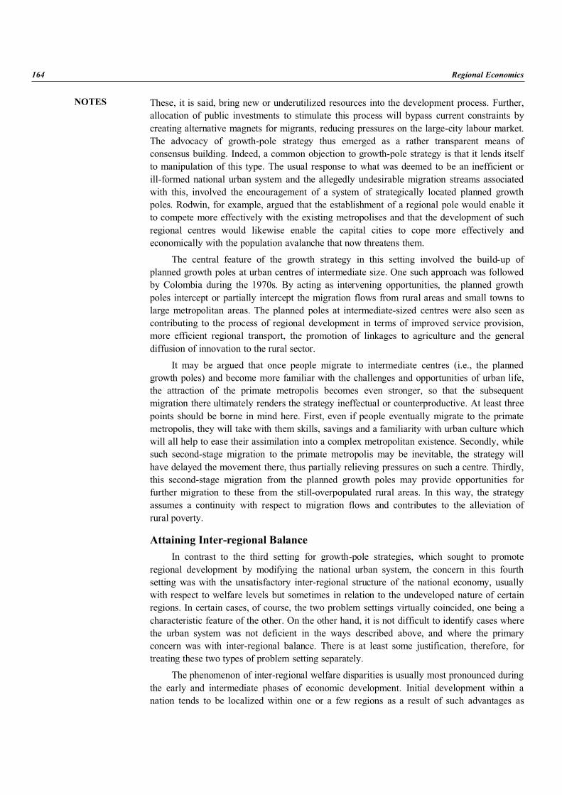
NOTES


These, it is said, bring new or underutilized resources into the development process. Further,allocation of public investments to stimulate this process will bypass current constraints bycreating alternative magnets for migrants, reducing pressures on the large-city labour market.The advocacy of growth-pole strategy thus emerged as a rather transparent means ofconsensus building. Indeed, a common objection to growth-pole strategy is that it lends itselfto manipulation of this type. The usual response to what was deemed to be an inefficient orill-formed national urban system and the allegedly undesirable migration streams associatedwith this, involved the encouragement of a system of strategically located planned growthpoles. Rodwin, for example, argued that the establishment of a regional pole would enable itto compete more effectively with the existing metropolises and that the development of suchregional centres would likewise enable the capital cities to cope more effectively andeconomically with the population avalanche that now threatens them.

The central feature of the growth strategy in this setting involved the build-up ofplanned growth poles at urban centres of intermediate size. One such approach was followedby Colombia during the 1970s. By acting as intervening opportunities, the planned growthpoles intercept or partially intercept the migration flows from rural areas and small towns tolarge metropolitan areas. The planned poles at intermediate-sized centres were also seen ascontributing to the process of regional development in terms of improved service provision,more efficient regional transport, the promotion of linkages to agriculture and the generaldiffusion of innovation to the rural sector.

It may be argued that once people migrate to intermediate centres (i.e., the plannedgrowth poles) and become more familiar with the challenges and opportunities of urban life,the attraction of the primate metropolis becomes even stronger, so that the subsequentmigration there ultimately renders the strategy ineffectual or counterproductive. At least threepoints should be borne in mind here. First, even if people eventually migrate to the primatemetropolis, they will take with them skills, savings and a familiarity with urban culture whichwill all help to ease their assimilation into a complex metropolitan existence. Secondly, whilesuch second-stage migration to the primate metropolis may be inevitable, the strategy willhave delayed the movement there, thus partially relieving pressures on such a centre. Thirdly,this second-stage migration from the planned growth poles may provide opportunities forfurther migration to these from the still-overpopulated rural areas. In this way, the strategyassumes a continuity with respect to migration flows and contributes to the alleviation ofrural poverty.

Attaining Inter-regional BalanceIn contrast to the third setting for growth-pole strategies, which sought to promote

regional development by modifying the national urban system, the concern in this fourthsetting was with the unsatisfactory inter-regional structure of the national economy, usuallywith respect to welfare levels but sometimes in relation to the undeveloped nature of certainregions. In certain cases, of course, the two problem settings virtually coincided, one being acharacteristic feature of the other. On the other hand, it is not difficult to identify cases wherethe urban system was not deficient in the ways described above, and where the primaryconcern was with inter-regional balance. There is at least some justification, therefore, fortreating these two types of problem setting separately.

The phenomenon of inter-regional welfare disparities is usually most pronounced duringthe early and intermediate phases of economic development. Initial development within anation tends to be localized within one or a few regions as a result of such advantages as

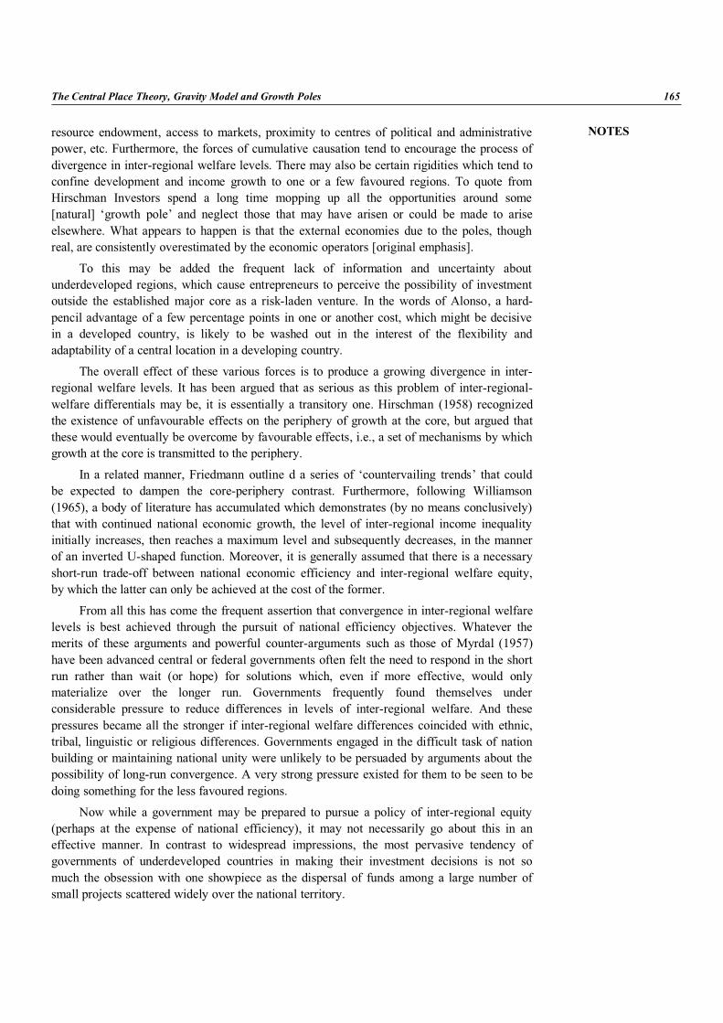
NOTES


resource endowment, access to markets, proximity to centres of political and administrativepower, etc. Furthermore, the forces of cumulative causation tend to encourage the process ofdivergence in inter-regional welfare levels. There may also be certain rigidities which tend toconfine development and income growth to one or a few favoured regions. To quote fromHirschman Investors spend a long time mopping up all the opportunities around some[natural] ‘growth pole’ and neglect those that may have arisen or could be made to ariseelsewhere. What appears to happen is that the external economies due to the poles, thoughreal, are consistently overestimated by the economic operators [original emphasis].

To this may be added the frequent lack of information and uncertainty aboutunderdeveloped regions, which cause entrepreneurs to perceive the possibility of investmentoutside the established major core as a risk-laden venture. In the words of Alonso, a hard-pencil advantage of a few percentage points in one or another cost, which might be decisivein a developed country, is likely to be washed out in the interest of the flexibility andadaptability of a central location in a developing country.

The overall effect of these various forces is to produce a growing divergence in inter-regional welfare levels. It has been argued that as serious as this problem of inter-regional-welfare differentials may be, it is essentially a transitory one. Hirschman (1958) recognizedthe existence of unfavourable effects on the periphery of growth at the core, but argued thatthese would eventually be overcome by favourable effects, i.e., a set of mechanisms by whichgrowth at the core is transmitted to the periphery.

In a related manner, Friedmann outline d a series of ‘countervailing trends’ that couldbe expected to dampen the core-periphery contrast. Furthermore, following Williamson(1965), a body of literature has accumulated which demonstrates (by no means conclusively)that with continued national economic growth, the level of inter-regional income inequalityinitially increases, then reaches a maximum level and subsequently decreases, in the mannerof an inverted U-shaped function. Moreover, it is generally assumed that there is a necessaryshort-run trade-off between national economic efficiency and inter-regional welfare equity,by which the latter can only be achieved at the cost of the former.

From all this has come the frequent assertion that convergence in inter-regional welfarelevels is best achieved through the pursuit of national efficiency objectives. Whatever themerits of these arguments and powerful counter-arguments such as those of Myrdal (1957)have been advanced central or federal governments often felt the need to respond in the shortrun rather than wait (or hope) for solutions which, even if more effective, would onlymaterialize over the longer run. Governments frequently found themselves underconsiderable pressure to reduce differences in levels of inter-regional welfare. And thesepressures became all the stronger if inter-regional welfare differences coincided with ethnic,tribal, linguistic or religious differences. Governments engaged in the difficult task of nationbuilding or maintaining national unity were unlikely to be persuaded by arguments about thepossibility of long-run convergence. A very strong pressure existed for them to be seen to bedoing something for the less favoured regions.

Now while a government may be prepared to pursue a policy of inter-regional equity(perhaps at the expense of national efficiency), it may not necessarily go about this in aneffective manner. In contrast to widespread impressions, the most pervasive tendency ofgovernments of underdeveloped countries in making their investment decisions is not somuch the obsession with one showpiece as the dispersal of funds among a large number ofsmall projects scattered widely over the national territory.

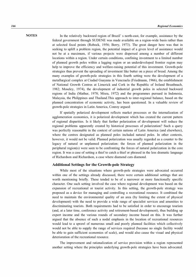
NOTES


In the relatively backward region of Brazil’ s north-east, for example, assistance by thefederal government through SUDENE was made available on a region-wide basis rather thanat selected focal points (Robock, 1956; Berry, 1973). The great danger here was that inseeking to uplift a problem region, the potential impact of a given level of assistance wouldnot be at a maximum, if various projects were dispersed among a number of differentlocations within a region. Under certain conditions, confining investment to a limited numberof planned growth poles within a lagging region or an underdeveloped frontier region mayhelp to improve the efficiency and welfare-raising potential of this investment. Growth-polestrategies thus prevent the spreading of investment like butter on a piece of bread. Among themany examples of growth-pole strategies in this fourth setting were the development of ametallurgical complex at Ciudad Guayana in Venezuela (Friedmann, 1966), the establishmentof National Growth Centres at Limerick and Cork in the Republic of Ireland Breathnach,1982; Moseley, 1974), the development of industrial growth poles in selected backwardregions of India (Mathur, 1978; Misra, 1972) and the programmes pursued in Indonesia,Malaysia, the Philippines and Thailand.This approach to inter-regional balance, based on theplanned concentration of economic activity, has been questioned. In a valuable review ofgrowth-pole strategies in Latin America, Conroy argued:

If spatially polarized development reflects market processes or the internalization ofagglomeration economies, it is polarized development which has created the current patternof regional disparities. Is it likely that further polarization of development will reduce theregional problems apparently created by historical processes of polarization? Such a querywas perfectly reasonable in the context of certain nations of Latin America (and elsewhere),where the centres designated as planned poles included natural poles. In other contexts,however, it would not be valid. Planned polarization was usually regarded as a counter to thelegacy of natural or unplanned polarization: the forces of planned polarization in theperipheral region(s) were seen to be confronting the forces of natural polarization in the coreregion. It was a case of setting a thief to catch a thief or phrased in the less dramatic languageof Richardson and Richardson, a case where diamond cuts diamond.

Additional Settings for the Growth-pole StrategyWhile most of the situations where growth-pole strategies were advocated occurred

within one of the settings already discussed, there were certain additional settings that areworth mentioning briefly. These tended to be of a narrower or more functionally specificcharacter. One such setting involved the case where regional development was based on theexpansion of recreational or tourist activity. In this setting, the growth-pole strategy wasproposed as a device for managing and controlling a recreational resource. It combined theneed to maintain the environmental quality of an area (by limiting the extent of physicaldevelopment) with the need to provide a wide range of specialist services and amenities todiscriminating tourists. Both requirements had to be satisfied in order to encourage tourism(and, at a later time, conference activity and retirement-based development), thus building upexport income and the various rounds of secondary income based on this. It was furtherargued that the absence of such a nodal emphasis in the location of recreational resourceswould lead to a sprawl of numerous small and poorly planned facilities which collectivelywould not be able to supply the range of services required (because no single facility wouldbe able to gain sufficient economies of scale), and would also cause the visual and physicaldeterioration of the recreational resource.

The improvement and rationalization of service provision within a region representedanother setting where the principles underlying growth-pole strategies have been advocated.

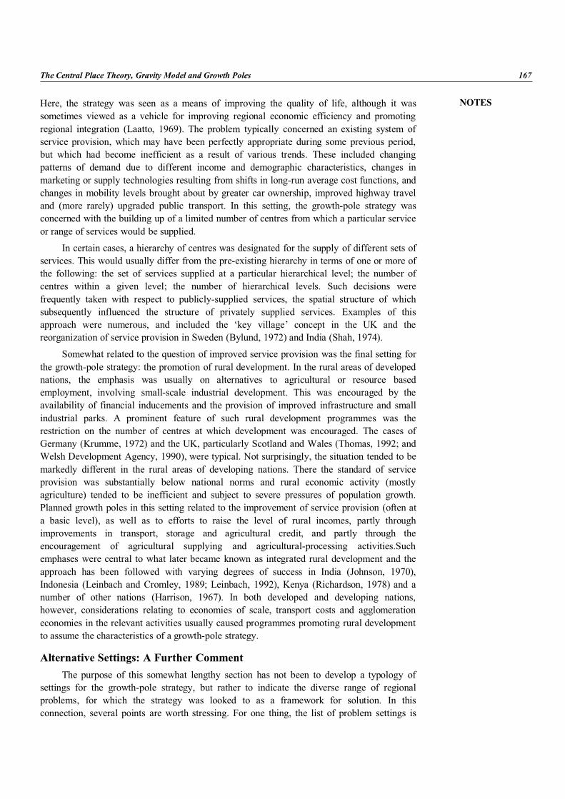
NOTES


Here, the strategy was seen as a means of improving the quality of life, although it wassometimes viewed as a vehicle for improving regional economic efficiency and promotingregional integration (Laatto, 1969). The problem typically concerned an existing system ofservice provision, which may have been perfectly appropriate during some previous period,but which had become inefficient as a result of various trends. These included changingpatterns of demand due to different income and demographic characteristics, changes inmarketing or supply technologies resulting from shifts in long-run average cost functions, andchanges in mobility levels brought about by greater car ownership, improved highway traveland (more rarely) upgraded public transport. In this setting, the growth-pole strategy wasconcerned with the building up of a limited number of centres from which a particular serviceor range of services would be supplied.

In certain cases, a hierarchy of centres was designated for the supply of different sets ofservices. This would usually differ from the pre-existing hierarchy in terms of one or more ofthe following: the set of services supplied at a particular hierarchical level; the number ofcentres within a given level; the number of hierarchical levels. Such decisions werefrequently taken with respect to publicly-supplied services, the spatial structure of whichsubsequently influenced the structure of privately supplied services. Examples of thisapproach were numerous, and included the ‘key village’ concept in the UK and thereorganization of service provision in Sweden (Bylund, 1972) and India (Shah, 1974).

Somewhat related to the question of improved service provision was the final setting forthe growth-pole strategy: the promotion of rural development. In the rural areas of developednations, the emphasis was usually on alternatives to agricultural or resource basedemployment, involving small-scale industrial development. This was encouraged by theavailability of financial inducements and the provision of improved infrastructure and smallindustrial parks. A prominent feature of such rural development programmes was therestriction on the number of centres at which development was encouraged. The cases ofGermany (Krumme, 1972) and the UK, particularly Scotland and Wales (Thomas, 1992; andWelsh Development Agency, 1990), were typical. Not surprisingly, the situation tended to bemarkedly different in the rural areas of developing nations. There the standard of serviceprovision was substantially below national norms and rural economic activity (mostlyagriculture) tended to be inefficient and subject to severe pressures of population growth.Planned growth poles in this setting related to the improvement of service provision (often ata basic level), as well as to efforts to raise the level of rural incomes, partly throughimprovements in transport, storage and agricultural credit, and partly through theencouragement of agricultural supplying and agricultural-processing activities.Suchemphases were central to what later became known as integrated rural development and theapproach has been followed with varying degrees of success in India (Johnson, 1970),Indonesia (Leinbach and Cromley, 1989; Leinbach, 1992), Kenya (Richardson, 1978) and anumber of other nations (Harrison, 1967). In both developed and developing nations,however, considerations relating to economies of scale, transport costs and agglomerationeconomies in the relevant activities usually caused programmes promoting rural developmentto assume the characteristics of a growth-pole strategy.

Alternative Settings: A Further CommentThe purpose of this somewhat lengthy section has not been to develop a typology of

settings for the growth-pole strategy, but rather to indicate the diverse range of regionalproblems, for which the strategy was looked to as a framework for solution. In thisconnection, several points are worth stressing. For one thing, the list of problem settings is

NOTES


not exhaustive, in the obvious sense that additional settings can be identified, although theseare likely to be of a rather specific nature. Also, the problems of a particular region maycontain elements of more than one setting, and mention has already been made of the possibleoverlap between modifying the national urban system and attaining inter-regional balance.Another overlap could involve the reviving of a depressed area and the encouragement ofregional deconcentration from a dominant metropolitan area, as in the case of CentralScotland in the 1960s (Great Britain, 1963). Furthermore, it is entirely possible for growth-pole strategies to be adopted simultaneously in regions with quite different problem settings.An obvious danger lurks here, to the extent that pursuing the strategy in one region may notbe consistent with the adoption of the strategy in another region with a different problemsetting. It is likely, however, that such a conflict would arise if alternative strategies wereapplied, conflicts of this kind being part of the more general problem of national ormultiregional co-ordination.

The Nature of the Growth-pole Strategy and its RationaleIn spite of the wide diversity of problem settings in which the growth-pole strategy has

been proposed, it is possible to identify the following set of characteristic features of thestrategy, this being common to all settings.

First, the strategy involves encouraging the growth of employment and populationwithin a region at particular locations or planned poles over some specified period. This doesnot necessarily imply that growth will be absent from other parts of the region, but theplanned poles are usually seen as the primary focus for regional investment, whether publicor private and whether based on a key industry, an industrial complex or some alternativeeconomic-activity set.

Secondly, the strategy imposes a definite limitation on the number of locations orcentres which are designated as planned poles and this will vary from setting to setting. Forexample, a policy aimed at stimulating rural development within a region might requirerelatively many planned poles, while a policy designed to attain inter-regional balance wouldinvolve relatively few. The limitation on pole frequency is also likely to be related to the typeof economic activity to be located within the region.

Thirdly, the strategy necessarily requires spatial discrimination or selectivity amonglocations. This discrimination is usually concerned with the identification of centres whichhave the potential for sustaining a given range of economic activity and is based on suchfactors as inter-regional or intra-regional locational advantage, hierarchical level within theurban system or (less satisfactorily perhaps) past growth record.

Fourthly, the strategy inevitably involves a modification of the spatial structure ofemployment and population within a region. Indeed, an important foundation of the growth-pole strategy is the proposition that the existing spatial structure represents an impediment toregional economic expansion, and that policy objectives can only be realized if inter alia thespatial structure is modified, usually in the direction of concentration. Such a modification ofthe spatial structure is primarily with respect to employment and, except for certain specialcircumstances (where reliance is placed on commuting), this will inevitably result in amodification of the spatial-structure of population.

It is possible, however, that the attempt at spatial-structure modification may be directedin the first instance to population, in the expectation that a more concentrated spatial structureof employment will evolve. All four of these characteristics are present to some degree in thevarious settings for the growth-pole strategy considered.

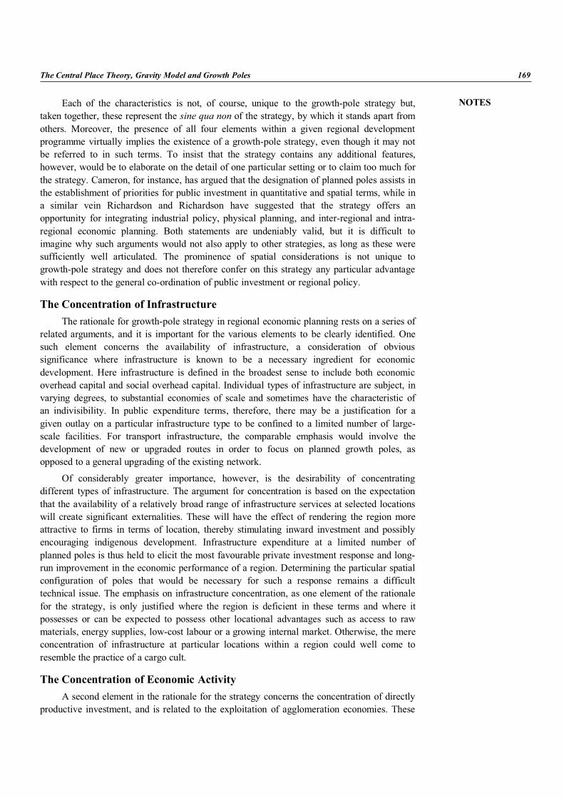
NOTES


Each of the characteristics is not, of course, unique to the growth-pole strategy but,taken together, these represent the sine qua non of the strategy, by which it stands apart fromothers. Moreover, the presence of all four elements within a given regional developmentprogramme virtually implies the existence of a growth-pole strategy, even though it may notbe referred to in such terms. To insist that the strategy contains any additional features,however, would be to elaborate on the detail of one particular setting or to claim too much forthe strategy. Cameron, for instance, has argued that the designation of planned poles assists inthe establishment of priorities for public investment in quantitative and spatial terms, while ina similar vein Richardson and Richardson have suggested that the strategy offers anopportunity for integrating industrial policy, physical planning, and inter-regional and intra-regional economic planning. Both statements are undeniably valid, but it is difficult toimagine why such arguments would not also apply to other strategies, as long as these weresufficiently well articulated. The prominence of spatial considerations is not unique togrowth-pole strategy and does not therefore confer on this strategy any particular advantagewith respect to the general co-ordination of public investment or regional policy.

The Concentration of InfrastructureThe rationale for growth-pole strategy in regional economic planning rests on a series of

related arguments, and it is important for the various elements to be clearly identified. Onesuch element concerns the availability of infrastructure, a consideration of obvioussignificance where infrastructure is known to be a necessary ingredient for economicdevelopment. Here infrastructure is defined in the broadest sense to include both economicoverhead capital and social overhead capital. Individual types of infrastructure are subject, invarying degrees, to substantial economies of scale and sometimes have the characteristic ofan indivisibility. In public expenditure terms, therefore, there may be a justification for agiven outlay on a particular infrastructure type to be confined to a limited number of large-scale facilities. For transport infrastructure, the comparable emphasis would involve thedevelopment of new or upgraded routes in order to focus on planned growth poles, asopposed to a general upgrading of the existing network.

Of considerably greater importance, however, is the desirability of concentratingdifferent types of infrastructure. The argument for concentration is based on the expectationthat the availability of a relatively broad range of infrastructure services at selected locationswill create significant externalities. These will have the effect of rendering the region moreattractive to firms in terms of location, thereby stimulating inward investment and possiblyencouraging indigenous development. Infrastructure expenditure at a limited number ofplanned poles is thus held to elicit the most favourable private investment response and long-run improvement in the economic performance of a region. Determining the particular spatialconfiguration of poles that would be necessary for such a response remains a difficulttechnical issue. The emphasis on infrastructure concentration, as one element of the rationalefor the strategy, is only justified where the region is deficient in these terms and where itpossesses or can be expected to possess other locational advantages such as access to rawmaterials, energy supplies, low-cost labour or a growing internal market. Otherwise, the mereconcentration of infrastructure at particular locations within a region could well come toresemble the practice of a cargo cult.

The Concentration of Economic ActivityA second element in the rationale for the strategy concerns the concentration of directly

productive investment, and is related to the exploitation of agglomeration economies. These

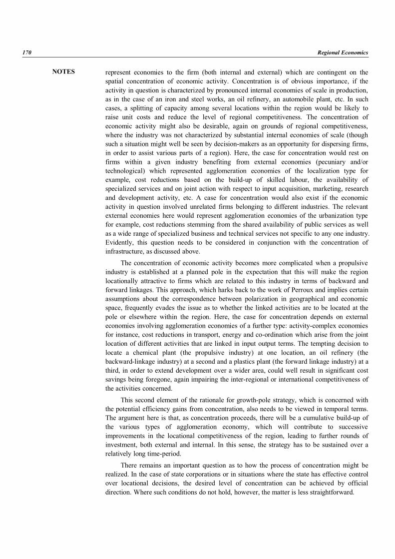
NOTES


represent economies to the firm (both internal and external) which are contingent on thespatial concentration of economic activity. Concentration is of obvious importance, if theactivity in question is characterized by pronounced internal economies of scale in production,as in the case of an iron and steel works, an oil refinery, an automobile plant, etc. In suchcases, a splitting of capacity among several locations within the region would be likely toraise unit costs and reduce the level of regional competitiveness. The concentration ofeconomic activity might also be desirable, again on grounds of regional competitiveness,where the industry was not characterized by substantial internal economies of scale (thoughsuch a situation might well be seen by decision-makers as an opportunity for dispersing firms,in order to assist various parts of a region). Here, the case for concentration would rest onfirms within a given industry benefiting from external economies (pecuniary and/ortechnological) which represented agglomeration economies of the localization type forexample, cost reductions based on the build-up of skilled labour, the availability ofspecialized services and on joint action with respect to input acquisition, marketing, researchand development activity, etc. A case for concentration would also exist if the economicactivity in question involved unrelated firms belonging to different industries. The relevantexternal economies here would represent agglomeration economies of the urbanization typefor example, cost reductions stemming from the shared availability of public services as wellas a wide range of specialized business and technical services not specific to any one industry.Evidently, this question needs to be considered in conjunction with the concentration ofinfrastructure, as discussed above.

The concentration of economic activity becomes more complicated when a propulsiveindustry is established at a planned pole in the expectation that this will make the regionlocationally attractive to firms which are related to this industry in terms of backward andforward linkages. This approach, which harks back to the work of Perroux and implies certainassumptions about the correspondence between polarization in geographical and economicspace, frequently evades the issue as to whether the linked activities are to be located at thepole or elsewhere within the region. Here, the case for concentration depends on externaleconomies involving agglomeration economies of a further type: activity-complex economiesfor instance, cost reductions in transport, energy and co-ordination which arise from the jointlocation of different activities that are linked in input output terms. The tempting decision tolocate a chemical plant (the propulsive industry) at one location, an oil refinery (thebackward-linkage industry) at a second and a plastics plant (the forward linkage industry) at athird, in order to extend development over a wider area, could well result in significant costsavings being foregone, again impairing the inter-regional or international competitiveness ofthe activities concerned.

This second element of the rationale for growth-pole strategy, which is concerned withthe potential efficiency gains from concentration, also needs to be viewed in temporal terms.The argument here is that, as concentration proceeds, there will be a cumulative build-up ofthe various types of agglomeration economy, which will contribute to successiveimprovements in the locational competitiveness of the region, leading to further rounds ofinvestment, both external and internal. In this sense, the strategy has to be sustained over arelatively long time-period.

There remains an important question as to how the process of concentration might berealized. In the case of state corporations or in situations where the state has effective controlover locational decisions, the desired level of concentration can be achieved by officialdirection. Where such conditions do not hold, however, the matter is less straightforward.

NOTES


On the surface at least, it would seem that, if the various types of agglomerationeconomies at the planned poles were significant, then private corporations would have anobvious incentive to concentrate there, unless there were compelling locational reasons fordoing otherwise. Yet the problem of unrelated investment decisions (taken over slightlydifferent periods, under different market conditions and with incomplete information) maywell result in an undesirably low level of concentration, with the attendant disadvantages. Inthese circumstances, there seems to be a case for securing the appropriate level ofconcentration by making any financial assistance to private corporations conditional upontheir location at the planned pole(s), although it has been claimed that this restriction isundesirable.

The Planned Poles and the RegionThere exists a third element in the rationale for the strategy, and this concerns those

parts of the region which have not been designated as planned growth poles. Here, however,the rationale for the strategy appears to follow two diverging paths. One view holds thatgrowth at the planned poles will be transmitted by a variety of mechanisms to the remainderof the region, the unstated assumptions being that growth in the rest of the region is not onlygreater than would occur under some alternative strategy, but is also greater than any possibledisadvantages caused by growth at the planned poles. An alternative view states that thespatial structure of the region undergoes a radical long run reshaping, by which growth at theplanned poles is accompanied (and partially facilitated) by a major redistribution ofpopulation and employment towards such centres. This view of the strategy inevitablyinvolves the running down, if not the virtual abandonment, of certain parts of the region, anapproach which is justified in terms of a more efficient utilization of the region’s existingfactor endowment. The presence of a labour force in sufficiently large pools consolidates theadvantage of low-cost labour and permits improvements in the provision of consumer andbusiness services.

All this helps to render the region more attractive to inward investment and under themost favourable of conditions may assist the process of indigenous development.

In this way, the focusing of population and employment on planned poles becomes themeans by which a more competitive spatial structure can be attained, leading to an improvedregional economic performance.

We thus have two contrasting views of the role of planned poles in relation to the rest ofthe region, a further reflection of the fact that the strategy has been proposed in a diversity ofsettings. It was sometimes the case, however, that the growth-pole strategy was designed withboth emphases in mind, i.e., the expectation of some favourable impact of the planned polesthroughout the region, as well as the encouragement of a more concentrated spatial structurefocusing on the planned poles. Such a mixing of emphases may have been appropriate incertain situations, but there were other occasions when it reflected an uncertainty on the partof planners or an unwillingness to come to terms with the underlying demands of the strategy.

The Rationale in ContextThese three categories of argument, which collectively form the rationale for the

growth-pole strategy, are insufficient for the policy-maker, however. To establish a rationalefor a strategy is neither to provide a justification for its adoption, nor to demonstrate itssuperiority over other strategies. The arguments are conditional, in as much that these arebased on assertions and suppositions which in any proposed application of the strategy would

NOTES


need to be demonstrated. And even if such arguments can be shown to be valid and consistentin a particular proposed application, there remain important questions which go beyond thescope of the rationale. These involve such issues as the budgetary requirements of thestrategy, the economic and administrative instruments by which it can be implemented, thedesirability of the anticipated outcomes in terms of intra-regional equity and balance, theexistence of secondary objectives of policy, the acceptability of the strategy, etc. More thananything else, it was the failure of the zealots (whether theorists or practitioners) to place therationale within the context of these other issues that led initially to the widespreadacceptance of the strategy.

4.5 SUMMARY

1. Central Place Theory (CPT) is an attempt to explain the spatial arrangement, sizeand number of settlements.

2. Christaller pointed out that the marketing principle is an awkward arrangement interms of connecting different levels of the hierarchy.

3. Christaller’s other suggested organizing principle was based upon the realizationthat from a political or administrative viewpoint centers it was unrealistic forcenters to be ‘shared’.

4. Rank size distribution, or the rank size rule (or law), describes the remarkableregularity in many phenomena, including the distribution of city sizes, the sizes ofbusinesses, the sizes of particles (such as sand), the lengths of rivers, thefrequencies of word usage and wealth among individuals.

5. The gravity model in economics was until relatively recently an intellectual orphan,unconnected to the rich family of economic theory. This review is a tale of theorphan’s reunion with its heritage and the benefits that continue to flow fromconnections to more distant relatives.


I. Fill in the Blanks1. From a modelling standpoint, __________ is distinguished by its __________ and

______ representation of economic interaction in a many country world.2. The __________ model drew on __________ with __________ of gravitation.

II. True and False1. Gravity has long been one of the most successful empirical models in economics.2. From a modelling standpoint, gravity is distinguished by its parsimonious and

tractable representation of economic interaction in a many country world.

III. Multiple Choice Questions1. A frictionless world implies that __________.

(a) Each good has the same price everywhere(b) Each good has different prices

NOTES


(c) Both (a) and (b)(d) Sometimes prices remain same and sometimes differ

2. Strategy of the structural gravity model research programme generates implicationslike __________.(a) Big producers have big market shares everywhere(b) Small sellers are more open in the sense of trading more with the rest of the

world(c) The world is more open the more similar in size are countries and the more

specialized are countries(d) All of the above

Short Answer Questions1. Explain in brief the term Traditional Gravity.2. Define the term ‘Frictionless Gravity’.

Long Answer Questions1. Explain in detail Gravity Model.2. Critically analyze Growth Poles.

4.7 KEY TERMS

Gravity ModelHierarchyRank Size DistributionThreshold


I. 1. gravity, parsimonious, tractable, 2. traditional gravity, analogy, Newton’s Law.II. 1. True, 2. True.

III. 1. (a), 2. (d).

UNIT IV: FEDERALISM AND ECONOMIC GROWTH

5Chapter


Federalism and Economic Growth: Theory of federalism, division of sources ofrevenue between the Central and State governments with special reference to Indianadjusting mechanism, problems of resources mobilization at the regional levelFederalismTheory of federalismDivision of sources of revenue between the Central and State governments withspecial reference to Indian adjusting mechanismProblems of resources mobilization at the regional level

Structure:5.1 Federalism5.2 Economic Growth5.3 Theory of Federalism5.4 Division of Sources of Revenue between the Central and State Governments with

Special Reference to Indian Adjusting Mechanism5.5 Problems of Resources Mobilization at the Regional Level5.6 Summary5.7 Self Assessment Questions5.8 Key Terms5.9 Key to Check your Answer

5.1 FEDERALISM

Federalism is a political concept in which a group of members are bound together bycovenant Latin: foedus, covenant) with a governing representative head. The term“federalism” is also used to describe a system of government in whichsovereignty is constitutionally divided between a central governing authority and constituentpolitical units (such as states or provinces). Federalism is a system basedupon democratic rules and institutions in which the power to govern is shared betweennational and provincial/state governments, creating what is often called a federation. Theterm federalist describes several political beliefs around the world. Also, it may refer to theconcept of parties; its members or supporters called themselves Federalists.

INFLUENCE OF FEDERALISM ININDIAN ECONOMY

NOTES

Influence of Federalism in Indian Economy 175

European vs. American FederalismIn Europe, “Federalist” is sometimes used to describe those who favour a common

federal government, with distributed power at regional, national and supranational levels.Most European federalists want this development to continue within the European Union.European federalism originated in post-war Europe; one of the more important initiativeswas Winston Churchill’s speech in Zurich in 1946.

In the United States, federalism originally referred to belief in a stronger centralgovernment. When the US Constitution was being drafted, the Federalist Party supported astronger central government, while “Anti-federalists” wanted a weaker central government.This is very different from the modern usage of “federalism” in Europe and the United States.The distinction stems from the fact that “federalism” is situated in the middle of the politicalspectrum between a confederacy and a unitary state. The US Constitution was written as areaction to the Articles of Confederation, under which the United States was a looseconfederation with a weak central government. Further, during the American Civil War,members of the Confederate States of America, which seceded in favor of a weaker centralgovernment, referred to pro-Union soldiers of the United States government as “Federals.”Thus, in the United States, “federalism” argued for a stronger central government, relative toa confederacy.

In contrast, Europe has a greater history of unitary states than North America, thus,European “federalism” argues for a weaker central government, relative to a unitary state.The modern American usage of the word is much closer to the European sense. As the powerof the Federal government has increased, some people have perceived a much more unitarystate than they believe the Founding Fathers intended. Most people politically advocating“federalism” in the United States argue in favour of limiting the powers of the federalgovernment, especially the judiciary.

In Canada, federalism typically implies opposition to sovereigntist movements (mostcommonly Quebec separatism).

The governments of Argentina, Australia, Brazil, India, and Mexico, among others, arealso organized along federalist principles.

Federalism may encompass as few as two or three internal divisions, as is the casein Belgium or Bosnia and Herzegovina. In general, two extremes of federalism can bedistinguished: at one extreme, the strong federal state is almost completely unitary, with fewpowers reserved for local governments; while at the other extreme, the national governmentmay be a federal state in name only, being a confederation in actuality.

In 1999, the Government of Canada established the Forum of Federations as aninternational network for exchange of best practices among federal and federalizing countries.Headquartered in Ottawa, the Forum of Federations partner governments include Australia,Brazil, Canada, Ethiopia, Germany, India, Mexico, Nigeria and Switzerland.

Some Christian denominations are organized on federalist principles; in these churchesthis is known as ecclesiastic or theological federalism.

Indian Federalism: The Government of India (referred to as the Union Government)was established by the Constitution of India and is the governing authority of a federalunion of 29 states and 7 union territories. Though, Andhra Pradesh was divided into twostates, Telangana and a residual Andhra Pradesh on 2 June 2014. Hyderabad, located entirelywithin the borders of Telangana, is to serve as joint capital for both states for a period of timenot exceeding ten years.

NOTES


In August 2014, the Government of Andhra Pradesh announced that Vijayawada willserve as the de facto administrative capital for Andhra Pradesh.

The government of India is based on a tiered system, in which the Constitution ofIndia delineates the subjects on which each tier of government has executive powers. TheConstitution originally provided for a two-tier system of government, the Union Government(also known as the Central Government), representing the Union of India, and the StateGovernments. Later, a third tier was added in the form of Panchayats and Municipalities. Inthe current arrangement, The Seventh Schedule of the Indian Constitution delimits thesubjects of each level of governmental jurisdiction, dividing them into three lists:

1. Union List includes subjects of national importance such as defence of the country,foreign affairs, banking, communications and currency. The Union Government alone canmake laws relating to the subjects mentioned in the Union List.

2. State List contains subjects of State and local importance such as police, trade,commerce, agriculture and irrigation. The State Governments alone can make laws relating tothe subjects mentioned in the State List.

3. Concurrent List includes subjects of common interest to both the Union Governmentas well as the State Governments, such as education, forest, trade unions, marriage, adoptionand succession. Both the Union as well as the State Governments can make laws on thesubjects mentioned in this list. If their laws conflict with each other, the law made by theUnion Government will prevail.

Asymmetric Federalism: A distinguishing aspect of Indian federalism is that unlikemany other forms of federalism, it is asymmetric. Article 370 makes special provisions forthe state of Jammu and Kashmir as per its Instrument of Accession. Article 371 makes specialprovisions for the states of Andhra Pradesh, Arunachal Pradesh, Assam, Goa, Mizoram,Manipur, Nagaland and Sikkim as per their accession or state-hood deals. Also one moreaspect of Indian federalism is system of President’s Rule in which the central government(through its appointed Governor) takes control of state’s administration for certain monthswhen no party can form a government in the state or there is violent disturbance in the state.

Coalition Politics: Although the Constitution does not say so, India is now amultilingual federation. India has a multi-party system,with political allegiances frequentlybased on linguistic, regional and caste identities, necessitating coalition politics, especially atthe Union Level.

Federalism as the Anarchist and Libertarian Socialist Mode of PoliticalOrganization: Anarchists are against the State but are not against political organization or“governance” — so long as it is self-governance utilizing direct democracy. The mode ofpolitical organization preferred by anarchists, in general, is federalismor confederalism. However, the anarchist definition of federalism tends to differ from thedefinition of federalism assumed by pro-state political scientists. The following is a briefdescription of federalism from Section I.5 of An Anarchist.

The social and political structure of anarchy is similar to that of the economic structure,i.e., it is based on a voluntary federation of decentralized, directly democratic policy-makingbodies. These are the neighbourhood and community assemblies and their confederations. Inthese grassroots political units, the concept of “self-management” becomes that of“self-government”, a form of municipal organization in which people take back control oftheir living places from the bureaucratic state and the capitalist class whose interests it serves.

NOTES


The key to that change, from the anarchist standpoint, is the creation of a network ofparticipatory communities based on self-government through direct, face-to-face democracyin grassroots neighbourhood and community assemblies [meetings for discussion, debate, anddecision-making].

Since not all issues are local, the neighbourhood and community assemblies will alsoelect mandated and recallable delegates to the larger-scale units of self-government in orderto address issues affecting larger areas, such as urban districts, the city or town as a whole,the county, the bio-region, and ultimately the entire planet. Thus, the assemblies willconfederate at several levels in order to develop and co-ordinate common policies to dealwith common problems.

This need for co-operation does not imply a centralized body. To exercise yourautonomy by joining self-managing organizations and, therefore, agreeing to abide by thedecisions you help make is not a denial of that autonomy (unlike joining a hierarchicalstructure, where you forsake autonomy within the organization). In a centralized system, wemust stress, power rests at the top and the role of those below is simply to obey (it matters notif those with the power are elected or not, the principle is the same). In a federal system,power is not delegated into the hands of a few (obviously a “federal” government or state is acentralized system). Decisions in a federal system are made at the base of the organizationand flow upwards so ensuring that power remains decentralized in the hands of all. Workingtogether to solve common problems and organize common efforts to reach common goals isnot centralization and those who confuse the two make a serious error – they fail to understandthe different relations of authority each generates and confuse obedience with co-operation.

Christian Church: Federalism also finds expression in ecclesiology (the doctrine of thechurch). For example, Presbyterian church governance resembles parliamentaryrepublicanism (a form of political federalism) to a large extent. In Presbyteriandenominations, the local church is ruled by elected elders, some of which are ministerial.Each church then sends representatives or commissioners to presbyteries and further toa general assembly. Each greater level of assembly has ruling authority over its constituentmembers. In this governmental structure, each component has some level of sovereignty overitself. As in political federalism, in presbyterian ecclesiology there is shared sovereignty.

Other ecclesiologies also have significant representational and federalistic components,including the more anarchic congregational ecclesiology, and even in more hierarchicalepiscopal ecclesiology.

Some Christians argue that the earliest source of political federalism (or federalism inhuman institutions; in contrast to theological federalism) is the ecclesiastical federalism foundin the Binle. They point to the structure of the early Christian Church as described (and tomany, prescribed) in the New Testament. This is particularly demonstrated in the Council ofJerusalem, described in Acts Chapter 15, where the Apostles and elders gathered together togovern the Church; the Apostles being representatives of the universal Church, and eldersbeing such for the local church. To this day, elements of federalism can be found in almostevery Christian denomination, some more than others.

Constitutional StructureDivision of Powers: In a federation, the division of power between federal and regional

governments is usually outlined in the constitution. It is in this way that the right to self-government of the component states is usually constitutionally entrenched. Component states

NOTES


often also possess their own constitutions which they may amend as they see fit, although inthe event of conflict the federal constitution usually takes precedence.

In almost all federations, the central government enjoys the powers of foreign policyand national defense. Were this not the case a federation would not be a single sovereign state,per the UN definition. Notably, the states of Germany retain the right to act on their ownbehalf at an international level, a condition originally granted in exchange for the Kingdom ofBavaria’s agreement to join the German Empire in 1871. Beyond this the precise division ofpower varies from one nation to another. The constitutions of Germany and the UnitedStates provide that all powers not specifically granted to the federal government are retainedby the states. The Constitution of some countries like Canada and India, on the other hand,state that powers not explicitly granted to the provincial governments are retained by thefederal government. Much like the US system, the Australian Constitution allocates to theFederal government (the Commonwealth of Australia) the power to make laws about certainspecified matters which were considered too difficult for the States to manage, so that theStates retain all other areas of responsibility. Under the division of powers of the EuropeanUnion in the Lisbon Treaty, powers which are not either exclusively of European competenceor shared between EU and state are retained by the constituent states.

Where every component state of a federation possesses the same powers, we are said tofind ‘symmetric federalism’. Asymmetric federalism exists where states are granted differentpowers, or some possess greater autonomy than others do. This is often done in recognition ofthe existence of a distinct culture in a particular region or regions. In Spain,the Basques and Catalans, as well as the Galicians, spearheaded a historic movement to havetheir national specificity recognized, crystallizing in the “historical communities” suchas Navarre, Galicia, Catalonia and the Basque Country. They have more powers than the laterexpanded arrangement for other Spanish regions, or the Spain of the autonomouscommunities (called also the “coffee for everyone” arrangement), partly to deal with theirseparate identity and to appease peripheral nationalist leanings, partly out of respectto specific rights they had held earlier in history. However, strictly speaking, Spain is not afederalism, but a decentralized administrative organization of the state.

It is common that during the historical evolution of a federation there is a gradualmovement of power from the component states to the centre, as the federal governmentacquires additional powers, sometimes to deal with unforeseen circumstances. Theacquisition of new powers by a federal government may occur through formal constitutionalamendment or simply through a broadening of the interpretation of a government’s existingconstitutional powers given by the courts.

Usually, a federation is formed at two levels: the central government and the regions(states, provinces, territories), and little to nothing is said about second or third leveladministrative political entities. Brazil is an exception, because the 1988 Constitutionincluded the municipalities as autonomous political entities making the federation tripartite,encompassing the Union, the States, and the municipalities. Each state is divided intomunicipalities (municípios) with their own legislative council (camara de vereadores) and amayor (prefeito), which are partly autonomous from both Federal and State Government.Each municipality has a “little constitution”, called “organic law” (lei organica). Mexico is anintermediate case, in that municipalities are granted full autonomy by the federal constitutionand their existence as autonomous entities (municipio libre, “free municipality”) isestablished by the federal government and cannot be revoked by the states’ constitutions.Moreover, the federal constitution determines which powers and competencies belong

NOTES


exclusively to the municipalities and not to the consultant states. However, municipalities donot have an elected legislative assembly.

Federations often employ the paradox of being a union of states, while still being states(or having aspects of statehood) in themselves. For example, James Madison (author ofthe US Constitution) wrote in Federalist Paper No. 39 that the US Constitution is in strictnessneither a national nor a federal constitution; but a composition of both. In its foundation, it isfederal, not national; in the sources from which the ordinary powers of the Government aredrawn, it is partly federal, and partly national. This stems from the fact that states in the USmaintain all sovereignty that they do not yield to the federation by their own consent. Thiswas reaffirmed by the Tenth Amendment to the United States Constitution, which reserves allpowers and rights that are not delegated to the Federal Government as left to the States and tothe people.

Organs of Government: The structures of most federal governments incorporatemechanisms to protect the rights of component states. One method, known as intrastatefederalism, is to directly represent the governments of component states in federal politicalinstitutions. Where a federation has a bicameral legislature, the upper house is often used torepresent the component states while the lower house represents the people of the nation as awhole. A federal upper house may be based on a special scheme of apportionment, as is thecase in the senates of the United States and Australia, where each state is represented by anequal number of senators irrespective of the size of its population.

Alternatively, or in addition to this practice, the members of an upper house may beindirectly elected by the government or legislature of the component states, as occurred in theUnited States prior to 1913, or be actual members or delegates of the state governments, as,for example, is the case in the German Bundesrat and in the Council of the European Union.The lower house of a federal legislature is usually directly elected, with apportionment inproportion to population, although states may sometimes still be guaranteed a certainminimum number of seats.

In Canada, the provincial governments represent regional interests and negotiatedirectly with the central government. A First Ministers conference of the prime minister andthe provincial premiers is the de facto highest political forum in the land, although it is notmentioned in the constitution.

Federations often have special procedures for amendment of the federal constitution. Aswell as reflecting the federal structure of the state, this may guarantee that the self-governingstatus of the component states cannot be abolished without their consent. An amendment tothe constitution of the United States must be ratified by three-quarters of either the statelegislatures, or of constitutional conventions specially elected in each of the states, before itcan come into effect. In referendums to amend the constitutions of Australia and Switzerland,it is required that a proposal be endorsed not just by an overall majority of the electorate inthe nation as a whole, but also by separate majorities in each of a majority of the states orcantons. In Australia, this latter requirement is known as a double majority.

Some federal constitutions also provide that certain constitutional amendments cannotoccur without the unanimous consent of all states or of a particular state. The US constitutionprovides that no state may be deprived of equal representation in the senate without itsconsent. In Australia, if a proposed amendment will specifically impact one or more states,then it must be endorsed in the referendum held in each of those states. Any amendment tothe Canadian constitution that would modify the role of the monarchy would require

NOTES


unanimous consent of the provinces. The German Basic Law provides that no amendment isadmissible at all that would abolish the federal system.

Other Technical Terms: Fiscal federalism – federalism involving the transfer of fundsbetween different levels of government.

Formal federalism (or ‘constitutional federalism’) – the delineation of powers isspecified in a written constitution.

Executive federalism (also known as ‘administrative federalism’).

Federalism as a Political Philosophy: The meaning of federalism, as a politicalmovement, and of what constitutes a ‘federalist’, varies with country and historicalcontext. Movements associated with the establishment or development of federations canexhibit either centralizing or decentralizing trends.

5.2 ECONOMIC GROWTH

Economic Growth: Economic growth is a long-term process involving a period ofmany decades. Economic growth is accompanied by substantial rise both in the totalpopulation as well as real national income. In other words, Economic Growth impliestransformation of an economy from a state of underdevelopment to a state of development,from an agrarian to a highly industrialized society, from a low saver to a high saver and froma predominantly rural to a highly urbanized society. This transformation is mainly reflected ina sustained and steady rise in national and per capita incomes. In the words of Peterson,Economic Growth involves an increase over time in the actual output of goods and servicesas well as an increase in the economy’s capability to produce goods and services. Therefore,Economic Growth implies increase in per capita income of the country at constant prices. Ahigher per capita income would mean that people are better off and enjoy a higher standard ofliving. The increase in national or per capita income must be maintained for a long time isimplicit in the theory of economic growth. Literally, economic growth means an increase inthe countries Net National Product (NNP).

Economic Development: The term economic development is a process whereby aneconomy’s real national income increases over a long period of time. Alternatively, the termeconomic development may be defined with reference to a set of criteria or values or desiredconditions in society. So, economic development is a normative concept. It means more thanwhat economic growth connotes. According to Streeten, development implies modernizationand modernization implies transformation of human beings. Development as an objective anddevelopment as a process both embrace a change in fundamental attitudes to life, work insocial, cultural and political institutions. Streeten views about development as an interrelatedprocess of several dimensions which include output and incomes, conditions of production,levels of living (i.e., nutrition, housing,health and education), attitudes to work, institutionsand policies. The well-known ‘Basic Needs Approach’ to development is derived from hisconcept. According to this approach, development is to be measured with reference to theextent to which the basic needs of the people are satisfied.

Differences between Economic Growth and Economic DevelopmentGrowth and development are often used synonymously in economic discussion. But

question is – What is economic growth? What is economic development? Thus, beforeexplaining in detail about economic growth in this chapter, let us first of all clear the basicconcept of this two important terms here.

NOTES


Factors Affecting Economic Growth: The primary driving force of economic growthis the growth of productivity, which is the ratio of economic output to inputs such as capital,labour, energy, materials and business services. Increase in productivity lowers the cost ofgoods, which is called a shift in supply. According to John W. Kendrick’s estimate, three-quarters of increase in US per capita GDP from 1889 to 1957 was due to increasedproductivity. Over the 20th century, the real price of many goods declined by over 90 percent.Lower prices create an increase in aggregate demand, but demand for individual goods andservices is subject to diminishing marginal utility. Additional demand is created by new orimproved products.

Demographic factors influence growth by changing the employment to population ratioand the labour force participation rate. Because of their spending patterns the working agepopulation is an important source of aggregate demand. Other factors affecting economicgrowth include the quantity and quality of available natural resources, including land.

Measuring Economic Growth: Measures of National Income and Output: Varietyof measures of national income and output are used in economics to estimate total economicactivity in a country or region, including gross domestic product (GDP), gross nationalproduct (GNP), net national income (NNI), and adjusted national income (NNI adjusted fornatural resource depletion). All are specially concerned with counting the total amount ofgoods as well as services produced within some ‘boundary’. The boundary is usually definedby geography or citizenship and may also restrict the goods and services that are counted. Forexample, some measures count only goods and services that are exchanged for money,excluding bartered goods, while other measures may attempt to include bartered goodsby imputing monetary values to them.

National Accounts: National accounts or national account systems (NAS) areimplementation of complete and consistent accounting techniques for measuring economicactivity of a nation, which include detailed underlying measures that rely on double-entryaccounting. Such accounting makes the totals on both sides of an account equal even thoughthey each measure different characteristics, for instance production and income from it. Asa technique, the subject is termed as national accounting or social accounting. Alternatively,national accounts as systems may be distinguished from the economic data associated withthose systems. While sharing several common principles with business accounting, nationalaccounts are based upon economic concepts. One conceptual construct for representing flowsof all economic transactions that takes place in an economy is a social accounting matrix withaccounts in every respective row-column entry.

National accounting has developed in tandem with macroeconomics from 1930s, withits relation of aggregate demand to total output through interaction of such broad expenditurecategories as consumption and investment. Economic data from national accounts are alsoused for empirical analysis of economic growth and development.

Economic Growth versus the Business Cycle: Economists differentiate betweenshort-run economic changes in production and long-run economic growth. Short-run variationin economic growth is known as business cycle. Business cycle is made up of booms anddrops in production that takes place over a period of months or even years. Usually,economists attribute the ups and downs in the business cycle to fluctuations in aggregatedemand.

In contrast, the topic of economic growth is concerned with the long-run trend inproduction due to structural causes like technological growth and factor accumulation.Business cycle moves up and down, creates fluctuations around the long-run trend ineconomic growth.

NOTES


5.3 THEORY OF FEDERALISM

Indian Federalism: A Critical AppraisalWith remarkable prescience, the framers of the Indian constitution have equipped the

Indian state to respond to the demands for autonomy through the double mechanism ofindividual and group rights, as well as the federal construction of political power.

During the first phase of India’s constitutional development, some of these instrumentswere useful in empowering political majorities below the level of the national state throughthe effective enactment of provincial administrations.

The second phase of constitutional development through the states reorganization of1956-57, which created linguistically homogeneous states and counter-balanced the likelychauvinism through the promotion of the tree language formula, requiring the use of Hindi,English, and the regional language, made it possible to institutionalize the multiculturalnature of the Indian state, albeit with regional divergences of successes and failures in itsimplementation.

In its third phase, the same process of constitutional development of federalism in the1990s, India has witnessed the deepening of the principle of power sharing by theconstitutional and statutory powers accorded to village councils after 1993. One extremepoint of view is that India is definitely unifederal. As Prof. K.P. Mukherjee contends thatIndian constitution is definitely unifederal or a unitary constitution. Likewise, K. Santhanamhas remarked that by means of this provision the fundamental principal that a federationdepends upon the territorial integrity of states seems to have been forgotten. K.V. Raoobserves that the Units are very weak compared with the Centre. According to him, whileArticles 1 and 2 guarantee the existence of the States and this granted by the Constitutionitself, the continued existence of the Units, and especially their inclusion in a particular partin the First Schedule, is at the mercy of the Centre, nay, at the mercy of a bare majority of theParliament (Article 4). The other extreme view is of designating India as extremely federal.Likewise, C.H. Alexandrowicz opines — It is undoubtedly a federation in which theattributes of sovereignty are shared between the Centre and the States. In between these twointerpretations, we have a plethora of moderate interpreters. Granville Austin advocates thethesis of co-operative federalism. He believes that the very concept of co-operativefederalism implies a strong Centre; provincial governments are largely administrativeagencies for central policies. Secondly, Prof. Morris Jones talks of Indian federalism asbargaining federalism. He says — whereas the emphasis in the Constitution is ondemarcation, that of political relations is on co-operative bargaining. He points out that theFinance Commission declined in relative importance as compared with the rise of a system ofmatching grants which are made under Article 282 of the Constitution. Hard competitivebargaining keeps on going between the Centre and States of getting these matching grants.

The new group of regional leaders of India, drawing on their power bases in the states,often consisting of people from India’s periphery (in terms of religion, elite caste status, orgeographic distance from the Centre), are able to generate a different and new construction ofthe Indian nation state. In terms of the actual policies of the state, the regionalists are muchmore willing and (in view of their social base) able to listen to the minorities, to regions withhistorical grievances, to sections of society that entered post-Independence politics withunsolved, pre-Independence grievances.

NOTES


The horizontal and vertical expansion of the federal process has brought greaterlegitimacy to the Indian state and cohesion to the India nation. Rather than grand design, theprocess has been based on a series of ad hoc decision, based on the perceived benefits of therespective political actors of the day, sometimes against the advice if specialists who havemade the conventional arguments based on the imperatives of modernization and the logic ofeconomic viability.

One important weakness of institutional design and the federal process is clearly thelack of effective mechanisms for a coordinated interest aggregation of states versus theCentral government. Co-ordination mechanisms, such as the informal conference of ChiefMinisters and to some extent, also the Interstate Council, have largely proven to be limited intheir effectiveness. Nevertheless, coordination among Chief Ministers belonging to partiesnot included in the Central government coalition has taken place, as have collusion andcoordination between the Central government and many of those Chief Ministers belongingto parties which support the Central government in the Lok Sabha. In its own way, therefore,the Indian experience with the unprecedented and unconventional expansion of the federalprinciple serves to enrich the theory of federalism in confirming or disconfirming receivedknowledge about the strengths and weaknesses of federal systems the world over.

5.4 DIVISION OF SOURCES OF REVENUE BETWEEN THE CENTRALAND STATE GOVERNMENTS WITH SPECIAL REFERENCE TOINDIAN ADJUSTING MECHANISM

In all federations of the world, the centre is financially stronger than the states.Allocation of resources has been done in a manner as to give the centre a proportionatelymuch larger share of revenues than that of states. Further, sources of revenue at the disposalof the federal authority are more elastic than those with the states. This has been so in olderfederations and almost all the new federations have copied this arrangement. The centralgovernment has responsibility for economic development and stability. Financial stability andstrength at centre is necessary for discharge of these functions. Centre has, therefore, beengiven fiscal powers appropriate for this purpose.

Under such circumstances, transfer of resources from centre to states are essential partof the financial arrangements in a federation. There are three problems which give rise to theneed for such transfers. Firstly, there is an imbalance of revenue between the centre and thestates. Allocation of the sources of revenue is such that those with the centre are more paying,e.g., customs and excises. Secondly, all states in a federation have not reached the same stageof development. There is not enough base for taxation in some states. Thirdly, welfare anddevelopment activities have to be undertaken by states, for which means available to them arenot adequate and transfer of resources from Centre become, indispensable. Transfers usuallytake three forms: (1) Division of proceeds of certain taxes, (2) Grants by the Centre to Statesand (3) Loans given by the Centre to the States.

1. Division of the Proceeds of Certain Taxes: Proceeds of certain taxes are sharedbetween centre and states. In India, this is done in respect of income tax and excise. In manycases, there are certain taxes levied and collected by centre but proceeds of those are whollydistributed to states. These taxes could as well be levied and collected by states but centralmanagement is for uniformity in rates and coverage. Estate duty in India is a standingexample. There are certain other taxes which are levied by centre but which are collected andappropriated by states.

NOTES


The sharing is so done that the centre has a larger share sufficient for its requirementsand rest is distributed among states. There are three principles which are suggested fordistribution:

(i) States’ share may be on the principle of compensation for loss of revenue onaccount of federalization and federal policies. This is difficult to determine,particularly in the case of federations that have come into being as a consequenceof devolution of powers by a unitary centre.

(ii) Another principle is requirement needs of the states. These may be measured interms of population or policies and schemes adopted by states.

(iii) Backwardness of a state may also be a criterion for which some kind of an index ofbackwardness has to be worked out.

Complete justice and satisfaction to all states is impossible under any system ofdistribution. There are always pulls and pushes from states for the adoption and rejection ofspecific criteria. It is difficult to estimate requirements of states by any objective criterion.Perhaps, best scheme is for a commission to go into the state budgets, examine their plans fordevelopment and welfare and only thereafter suggest a suitable basis for distribution.

Distribution of tax revenues has certain disadvantages. Sometimes, rates of federal taxeshave to be kept unduly high to meet financial requirements of states. Other effects of thesetaxes are ignored. Further, while collecting, government incurs all unpopularity while statesthat receive shares get benefits. There is also no inducement for states to effect economies intheir expenditure.

2. Grants by the Centre to the States: Sometimes transfers take the form of grants.These are given primarily on the basis necessity of the states. Requirements have to becarefully estimated in relation to the resources of the states and grants are given to them.Requirements are measured in terms of population, percentage of collection, plans for welfareand development, and backwardness of states. These grants bring about a certain measure ofuniformity in resources available to states.

Grants are given to enable centre to exercise a certain measure of influence uponpolicies and schemes adopted by states. Centre can persuade units to adopt measures whichserve certain national purposes. Centre may also encourage grant receiving states to adoptschemes for their own benefit but which fit into general national plan.

Grants are based on two principles. One is authority transferring resources may retainresponsibility for their proper use. These are called ‘Conditional Grants’ and are given forspecific purposes. Other, ‘Unconditional Grants’ are given unconditionally but are to be spentin conformity with general principles of sound finance. Actual arrangements may be between,these two extremes. Centre gives both these grants. There are some grants to which nospecific conditions are attached. There are others which have to be spent by states for specificpurposes such as education, public health, housing, improvements of certain industries, etc. Indeveloping countries, some grants are given to implement specific programmes ofdevelopment.

3. Loans Given by the Centre to the States: States raise loans in the capital market,but they also get short-term and long-term loans from the central government. Loans may befor specific schemes or for general purposes. Like other kinds of transfer of resources, thisform also necessitates a central watch over the purpose and use for which states borrow.

NOTES


5.5 PROBLEMS OF RESOURCES MOBILIZATION AT THEREGIONAL LEVEL

Regarding demarcation of sources of revenue between centre and state, yet, financialarrangement between two are utmost important. As governments have their own allocatedfunctions, thus, they must possess sufficient or adequate resource to fulfill those needs.Alternatively, division of function pre-supposes division of resources. Constitutions of eachfederal state has distinct provision in this regard.

So far as basis of such division of resources are concerned, taxes and other sourcesprovides as base extending over entire nation, which mark its impact upon economic life of acountry included in the federal list. But, on contrary, other taxes those are based in individualstates and impacts of that seldom crosses beyond boundaries of a state are allocated in thatrespective state only. For instance, suppose customs duties which is related to trade of entirecountry are generally a central head of revenue. But taxes on land and other immovableproperty which is concerned to states only are usually sources of revenue in the hands ofrespective states only.

Distribution of resources in all federations aims at providing fiscal independence to allgovernments. Central and state authorities are given sources of income to fulfill their needs.Government should manage its resources efficiently to make its optimum utilization. Alongwith this, it should also maintain expenditure at a specific level so that it remains within themean available to it. It shows a sense of responsibility at the hand of units which is inevitablefor effective operations of federal system.

Financial arrangement in most federation in fact desirable from both economic as wellas political point of view. It makes units dependent upon centre and reduces fiscal autonomyto a mere ideal, which is difficult to achieve. Therefore, various adjustments are requiredbesides a mere distribution of revenue resources have to be in financial relations betweencentre and state units.

India has a federal form of Government, and hence federal finance system. Essence of afederal form of Government is that Central and State Governments should be independent ofeach in their respective, constitutionally demarcated spheres of action. Once the functions ofthe Governments are spelt out, it becomes equally important that each Governments shouldbe provided with sources of raising adequate revenue to discharge functions entrusted to them.For successful operation of federal form of Government financial independence and adequacyform the backbone.

Evolution of the finance system in India can be traced to the Government of India Act,1935. This Act was based upon general principle of financial independence for provinces.The constitution of India accepted this basic principle of federal finance and apart from thattried to achieve a few more principles among them first and the foremost is achievement of afinancially strong Centre. This is done by adopting the following measures: (a) Powers ofconcurrent taxation has been avoided; (b) Centre has been assigned more elastic and highyielding sources of revenues; (c) Centre has been given the subjects of money ana banks,currency and coinage; and powers to resort to deficit financing; (d) Centre has been providedwith certain exclusive sources of revenue; and (e) Residuary powers lies with the centre.

Secondly, the constitution has divided the various functions into three lists, viz.,(a) Union List, (b) States’ List and (c) Concurrent List. Financial powers have likewise beendivided between the Centre and the States.

NOTES


Thirdly, the constitution has made provision for transfer of resources. This is to beachieved by three means, viz., (a) tax sharing, (b) grants and (c) loans. These are sometimesreferred as “balancing factors” to correct inter-regional inequalities of income. One basicprinciple of federal finance is functions and resources should go together. However, in mostfederation, there is always a gap between functions to be discharged and financial resourcesneeded to discharge them. Hence, regional imbalances constitute a source of conflict and thisconflict is solved by the use of the balancing factors.

Fourthly, there exists a flexibility in transfer of resources. The reason is, resource aretransferred from the Centre to the States according to recommendations of the financecommission constituted by the President under the provisions of Article 280 of theconstitution. The Commission does not have any set procedure to go by. It has to make itsown choice. It lends flexibility to the system. Appointment of the Finance Commission is ofgreat importance for it enables the financial relation between the Centre and the States to bealtered in accordance with changes in need and circumstances.

Constitutional provisions relating to federal finance are segregated into three broadheads: i.e., (A) distribution of financial powers, (B) mechanism of resource transfers and(C) finance commissions.

A. Distribution of Financial Powers: The constitution makes a clear division offinancial resources between Centre and States. Sources of revenue can be grouped under twoheads, viz., (a) Sources of revenue for Centre and (b) Sources of revenue for States.

Sources of revenue to Centre are: (1) sources of tax revenue; and (2) sources of non-taxrevenue. Sources of tax revenue include 12 items like taxes on income other than agriculturalincome, corporation tax etc. The non-tax resources are: (1) borrowings; (2) income fromGovernment undertakings and monopolies; (3) income from Government property andincome arising out of the exercise of various Governmental functions and rights; (4) interestearnings on loans as well as advances to State Governments’ commercial and non-commercialundertakings; (5) gifts, donations etc; (6) fees in respect of any of the matters in the UnionList but not including fees taken in any court; and (7) fees taken in the Supreme court.

Similarly, the sources of revenue to the State Governments can be divided into:(a) sources of tax revenue; and (b) sources of non-tax revenue. Under constitution, Stateshave been given independent tax powers and the State list contains 19 items like land revenue,taxes on agricultural income, sales tax etc. The non-tax revenue includes: (a) fees taken in allcourts except the Supreme court; (b) income from undertakings owned partly or fully byrespective State Governments; (c) income earned from property owned by State Governments;(d) borrowings from within the country; (e) royalty from mines, forests, etc.; (f) grants-in-aidfrom centre; and (g) other grants from the Central Government.

Various taxes imposed by the Central Government are divided as follows:1. Taxes and duties which accrue wholly to the Union Government, e.g., customs

duties including export duties, corporation taxes etc.2. Taxes levied and collected by the Union but which may be shared with States

(Article 272 of the constitution).3. Taxes and duties levied and collected by centre but the proceeds of which are

assigned to States (Article 269 of the constitution), e.g., succession duty in respectof property other than agricultural land, terminal tax etc.

4. Taxes and duties levied by Centre but collected and appropriated by Stateconcerned (Article 268 of the constitution), e.g., stamp duties and excise duties,duties on medicinal and toilet preparations etc.

NOTES


This sort of the division of tax powers reflects on operational distinction made betweenlevying, collection and appropriation of tax proceeds. Each part has been decided on the basisof maximum efficiency expected under the constitution.

B. Mechanism of Resource Transfer: Important means of resource transfer are:(a) assignments; (b) tax-sharing; (c) grants-in-aid and (d) loans.

C. Finance Commissions: Specific provision has been made in the constitution for theappointment of a finance commission every five years or earlier. Under Section 280 of theconstitution, the President is empowered to appoint a finance commission at the expiry ofevery fifth year or earlier which shall consist of a chairman and four other members.

The finance commission makes recommendations to the President in regarding:(1) distribution of net proceeds of taxes to be shared between Union and States and allocationof shares of such proceeds among States; (2) principles which should govern the grants-in-aidto the revenues of States out of consolidated Fund of India; and (3) any other matter thefinance commission may deem fit. Important recommendations of all the ten commissions sofar reported have been accepted and acted upon by the Central Government, in the spirit ofthe constitution.

Centre-State Conflict on Finances: Financial relations between Centre and States areof vital importance for smooth functioning of a federation. Since last few years, there hasbeen growing conflict and tension between Indian Union and States. This conflict has beenaggravated by political and ideological differences among different parties governing theCentre and States. In the first place, the financial provisions of the constitution gave veryextensive financial resources to the Union and on the other hand, State Governments weregiven important responsibilities but inelastic and unproductive resources. This has been amajor reason of conflict between the Centre and States.

Secondly, under the weight of successive plans of economic and social development,there is a growing divergence between responsibilities arising from original distribution ofpowers and fiscal capacities between the Union and States.

Thirdly, there have been serious regional imbalances in economic development so muchso that some States have been left behind while others have made considerable economicprogress.

However, it must be stated that the amount of imbalance between regions is inevitablein a large country like ours. But Central Government did not use its financial resources or itspolicy of economic planning to bring about balanced development of all regions. Naturally,the backward and neglected States clamour for more powers and more financial resources.

Finally, the Indian Constitution provided for inter-governmental grants and loans, sothat the Centre might come to the help of those States which were in difficulties and also tobring about balanced development among different regions. Use of grants and loans in thelast 40 years or so, however, has resulted in complete domination and control of the States bythe Centre and utter dependence, and to a certain extent even financial irresponsibility andindiscipline on the part of the States. A stage has now been reached that while Centre-Statesfinancial relations will have to be reviewed thoroughly. The Thavaraj Committee (Report ofthe Taxation Enquiry Committee, Kerala government), the Rajamannar Committee onCentre-State relations appointed by the DMK Government of Tamil Nadu and the documenton Centre-State relations adopted by the West Bengal cabinet led by the CPI(M) UnitedFront — all these have the same theme, i.e., political and financial autonomy for States anddrastic restriction upon power as well as financial resources of the Centre.

NOTES


5.6 SUMMARY

1. Federalism is a political concept in which a group of members are bound togetherby covenant Latin: foedus, covenant) with a governing representative head.

2. Federalist is sometimes used to describe those who favour a common federalgovernment, with distributed power at regional, national and supranational levels.

3. In Canada, federalism typically implies opposition to sovereigntist movements(most commonly Quebec separatism).

4. The term economic development is a process whereby an economy’s real nationalincome increases over a long period of time.

5. The primary driving force of economic growth is the growth of productivity, whichis the ratio of economic output to inputs such as capital, labour, energy, materialsand business services.


I. Fill in the Blanks1. A distinguishing aspect of Indian federalism is that unlike many other forms of

federalism, it is __________.2. In a federation, the division of power between __________ and __________ is

usually outlined in the constitution.

II. True and False1. In almost all federations, the central government enjoys the powers of foreign

policy and national defense.2. Usually, a federation is formed at two levels: the central government and the

regions (states, provinces, territories), and little to nothing is said about second orthird level administrative political entities.

III. Multiple Choice Questions1. In economics, a production-possibility frontier (PPF), sometimes called __________.

(a) Production-possibility curve(b) Production-possibility boundary curve(c) Product transformation curve(d) All of the above

2. Economic growth is __________.(a) A long-term process involving a period of many decades(b) A short-term process(c) A periodic study(d) None of the above

Short Answer Questions1. Explain in brief the term ‘Economic Growth’.2. What are the measures of the economic growth?

NOTES


Long Answer Questions1. Critically analyze the term ‘Federalism’. What are its constitutional structure?2. Explain the neo-classical growth model.

5.8 KEY TERMS

EcclesiologiesFederalismFederalistProduction-possibility frontier


I. 1. asymmetric, 2. federal, regional governments.II. 1. True, 2. True.

III. 1. (d), 2. (a)

UNIT V: STABILIZATION AND GROWTH

6Chapter


Regional aspects of stabilization and growth policy Post- war regional cyclical behaviour and policy measure for stabilization Theories to explain regional differences in growth Fiscal programmes Tax Transfer programmes Fiscal responses of power level governments Regional orientation to policy programmes and central responsibility

Structure:6.1 Regional Aspects of Stabilization and Growth Policy6.2 Post -war Regional Cyclical Behaviour and Policy Measure for Stabilization6.3 Theories to Explain Regional Differences in Growth6.4 Fiscal Programmes6.5 Tax6.6 Transfer Programmes6.7 Fiscal Responses of Power Level Governments6.8 Regional Orientation to Policy Programmes and Central Responsibility6.9 Summary6.10 Self Assessment Questions6.11 Key Terms6.12 Key to Check Your Answer

6.1 REGIONAL ASPECTS OF STABILIZATION AND GROWTHPOLICY

Indian Economy stabilizes, but high inflation, slow growth key concerns India hasrestored macroeconomic and financial stability, but structural impediments to growth andpersistently high inflation remain key concerns. Over recent months, India has takensubstantive measures to narrow external and fiscal imbalances, tighten monetary policy,

REGIONAL DISPARITY ANDSTABILIZATION MEASURES

NOTES

Regional Disparity and Stabilization Measures 191

move forward on structural reforms and address market volatility. This has reduced itsvulnerability to shocks. Though spillovers from global financial market volatility continue topose a significant risk, Indian economy is now better placed to handle financial shocks. Thecurrent account deficit has contracted, the fiscal deficit target has been met and investmentproject approvals are accelerating. In addition to that, India has significant foreign exchangereserves to deploy in the event of external financing pressures. Exchange rate flexibility, atightening of liquidity conditions and limited foreign exchange interventions, had servedIndia well in responding to the present volatility.

Handling External Pressures: The report stressed the need to foster an environmentconducive to foreign direct investment to finance India’s current account deficit. In the eventof a resurgence of market volatility, the IMF stressed the importance of a well-communicatedpackage of policy measures to minimize disruptive movements in the currency and bolstermarket confidence. This would involve continued flexibility in the rupee, complemented bythe judicious use of reserves, tightening of monetary conditions, additional fiscalconsolidation efforts, and further easing of constraints on capital inflows.

Growth Eases: India’s growth, although among the highest in the world, has slowed inthe last two years. Growth is projected at 4.6 percent in 2013-14, but with a modest pick up to5.4 percent in 2014-15, helped by slightly stronger global growth, improving exportcompetitiveness, a favourable monsoon and a confidence boost from recent policy actions.India’s growth is expected to rise to its medium-term growth potential of about 6¾ percentonce recently approved investment projects are implemented and as global growth improves.Several important policy decisions have been made that should help revive investmentactivities, so that India can easily go back to an 8 percent growth trajectory if furtherstructural reforms, particularly in the fields of energy, agriculture and also the labour market.

Inflation Remains Elevated: Persistently high inflation is a key macroeconomicchallenge for India. Over the past several years, it has induced double-digit inflationexpectations and given rise to a high demand for gold. It has also eroded households’financial savings and undermined the stability of the rupee. Achieving a sustained reductionin inflation requires a tightening of the monetary stance, possibly over a protracted period. Itwill also be critical in achieving sustained, robust and inclusive growth. Food and fuel priceshocks propagate rapidly into core inflation and inflation expectations and wage formationare closely linked to CPI inflation.

Challenges and Policy Priorities: The IMF in its report commended the authorities’resolve to meet the budget deficit target despite slowing growth, but highlighted the need toimprove the quality of fiscal consolidation and make it more growth friendly. While themedium-term fiscal targets and resulting pace of consolidation are broadly appropriate,measures still need to be articulated and implemented to underpin the targeted fiscaladjustment. The report praised the progress made in tying India’s social safety net to theAadhaar (India’s Unique Identification Programme). The report said that achieving durablemedium-term fiscal adjustment will require more efficient taxation (including through theintroduction of the goods and services tax) and better allocation of spending (includingthrough reforms to fuel and fertilizer subsidies).

Further, raising the tax-to-GDP ratio to the pre-crisis level and reforming fuel andfertilizer subsidies will help reorient spending toward social priorities in health and education.According to the IMF’s assessment, India’s financial system remains well capitalized andsupervised, but slowing growth is highlighting corporate vulnerabilities and leading todeteriorating bank asset quality.

NOTES


IMF in its report welcomed the Reserve Bank of India’s recent initiatives to increaseprovisioning and capital requirements for bank lending to firms with sizeable foreigncurrency exposures and for improving the recognition of restructured advances on bankbalance sheets. Although no firm has come under severe stress so far, there is a keyinformation gap about the extent of unhedged foreign currency exposure of large firms,which needs to be rectified. Improvements in the legal and institutional insolvencyframework will also help deepen domestic capital markets.

6.2 POST-WAR REGIONAL CYCLICAL BEHAVIOUR AND POLICYMEASURE FOR STABILIZATION

Economic Fluctuations and Stabilization Policies (Post-war): Growth, stability anddistribution are the three principal concerns of economics. Since economics deals with thematerial well-being alone, the growth is defined in terms of the growth in real nationalincome, the stability in terms of the fluctuations in real national income or in the rate ofunemployment and in the (general) price level (inflation or deflation) and the distribution interms of the income distribution across households. Economists are unanimous in eachcountry aiming at a high growth rate, high stability and a fair, though not equal, distribution.But, most economists believe that the growth and price stability are incompatible goals in theshort run (Phillips’ curve) and thus, an ideal mix of the two is a debatable issue. The famousKuznets’ curve suggests that the growth and desired income distribution do not always movein tandem. The basic purpose of this discussion is basically addressed to economicfluctuations and their monitoring through the application of stabilization policies. Time seriesdata on economic fluctuations and the indicators of stabilizing policies in selected countriesare analyzed to examine the depth and spread of these fluctuations and the actual uses of thecorresponding policies. Inherent limitations of these policies are highlighted to appreciatetheir less than perfect role in taming business cycles.

Economic Fluctuations: Economic fluctuations are fact of life. All countries havesuffered from these, though the booms and busts have not always synchronized acrosscountries and neither the length nor the amplitude have been uniform. The average growthrate in these countries during the last about 40 years (1964-1997) has fluctuated between thelow of 2.3 percent in UK and the high of 9.2 percent in China, with the standard deviations of2.2 percent and 6.7 percent, respectively. For the world as a whole, while the average growthrate during the said period stood at 3.7 percent, the standard deviation of that turned out to be1.4 percent, giving a coefficient of variation of 38 percent. These indicate a fairly high degreeof volatility both over space and time. The maximum fluctuations in the growth rate were inChina, in the unemployment rate in UK, and in the inflation rate in India. In India, thedrought of 1979-80 (when the agriculture output fell by 12 percent) left that year the worstwith a negative growth rate of 6 percent and the mild reforms induced prosperity (whenindustrial output went up by 9.6 percent and finance, insurance, real estate and businessservices output was up by 11.4 percent) of the second half of the 1980s took the growth rateto its peak rate of around 10 percent in 1988-89. Some striking examples of extremefluctuations in the globe are cited below:

(a) The Great Depression of 1929-33 was fairly widespread across all countries. Duringthese four years, the GDP fell by about 29 percent in USA, 22 percent in Australia,18 percent in Czechoslovakia, 16 percent in Germany, 11 percent in each of France and

NOTES


Hungary, 9 percent in Sweden, 6 percent in UK and so on. The unemployment rates werehigh accordingly and most countries had experienced fairly high rates of deflation.

(b). The hyper-inflation (inflation over 1000 percent/year) plagued several Europeancountries, including Germany, Hungary, Austria and Poland, during the 1920s and againHungary during August 1945 to July 1946. Several Latin American countries, includingArgentina, Bolivia, Brazil, Nicaragua, Peru and Ukraine, have suffered from this diseaseduring the 1980s and 1990s.

(c) The stagflation during 1974-75 and 1979-82 was fairly widespread throughout theworld. Growth rate in the world output fell monotonously from 5.8 percent in 1973 to0.7 percent in 1975 and from 4.1 percent in 1978 to 0.4 percent in 1982. The world inflationrate stood at the two-digit levels in all these years. Several countries including USA and UKhad experienced negative growth rates in most of these years and the rest had lower than theirrespective trend rates in all these years. Most of the countries had suffered a two-digitinflation rate or a high one-digit rate.

(d) The fast growing prosperity was witnessed in Japan during the 1950s and 1960s.The Japanese economy is currently suffering from recession for over a decade. China hadexperienced a relatively high growth rate (two-digit level) during the most of the 1960s(barring 1967, during the worst recession), and the 1980s and 1990s. USA suffered the worstrecession after the Great Depression during 1979-82 but has performed reasonably wellduring the most of the 1990s. India has had a negative growth rate in 1956-57, 1964-65,1972-73, and 1979-80 (maximum at –6.0 percent) and a maximum growth rate of about10 percent in 1988-89. Most of the South-East Asian nations have achieved high growth ratesduring 1986 through 1996 until they were caught up by the recent financial crisis. Thebusiness cycles are found in Europe as well as the growth rates in those countries were eithernegative or low during the periods of stagflation (1974-75, 1979-82) as well as the early1990s and better in most other years. African countries and Latin American countries havewitnessed even worse cycles. The world recorded the highest growth rate at 6.2 percent in1964 and the lowest at 0.4 percent in 1982. In general, the 1980s and 1990s have been thedecades of a relatively good performance in most countries.

(e) Since the early 2001, most regions in the world are experiencing a recession, whichis in terms of a fall in the growth rate rather than a negative growth rate. This recession, likethe Great Depression of the early 1930s, and the stagflation of the mid-Seventies and earlyEighties is well spread across countries. However, the inflation rate has been quite modestlately in most countries. The unemployment and inflation further demonstrate the recurrenceof business cycles. According to the Arthur Okun’s law, the unemployment figures are justthe mirror image of the growth rate. The average inflation rate during 1964-2000 fluctuatedbetween 3.2 percent in Germany and 9.1 percent in India, with a standard deviation of1.8 percent and 2.8 percent respectively. The said figures for the world turned out to be11.1 percent and 5.9 percent, respectively. Therefore, the standard deviation of inflation wasfairly high as well.

3. Fluctuations in the real income and inflation rate have not been uniform through thevarious cycles. During the great depression, both the real income as well as the price fell.During the stagflation, the former fell while the latter rose. The same trend was witnessed,though at very different rates, during the hyper-inflation. During the last decade, theprosperity was accompanied with mild inflation. While inflation was perhaps the number oneeconomic ill during the stagflation and hyper-inflation, currently it is very much within thedesired range in most parts of the world.

NOTES


4. The fundamental factors behind these fluctuations are shocks in aggregate demand(AD) and aggregate supply (AS). These can be caused by changes in one or more of theexogenous variables (policy or non-policy ones) and the behavioural parameters of thedecision-makers, viz., consumers, input suppliers and firms. The non-policy variables thataffect AD include autonomous components of consumption, investment, export and imports,which, in turn, are guided by the confidence and expectations of consumers and firms, bothdomestic and foreign. The policy variables that have bearings on AD include money supply(or the high-powered money), government fiscal operations like government expenditure,taxation and transfer payments, and the foreign exchange rate, tariffs and quotas. Theclassists (supply siders) believe that direct taxes (personal income tax, corporate tax and therebates on saving and investment) affect AS as well, through incentives or disincentives tosupply more labour and save and invest more or less.

Besides, the behavioural parameters affecting AD include propensities to consume orsave, invest and import, interest sensitiveness of investment and money demands, priceelasticities of import and export, etc. Workers’ leisure-work preference, firms’ attitudetowards risk and profit, industrial relations and riots, etc. constitute the behaviouralparameters that affect AS. While the behavioural parameters are fairly constant in the shortrun, the non-policy and policy variables do change even in the short run. Therefore, the shiftsin AD and AS could be caused by a variety of factors even in the short run and any one ormore of them could have triggered or reinforced a particular contraction or recovery.

Economists are unanimous with regard to the downward sloping of the AD curve, whichis caused by the Keynesian, Pigou and international trade effects, though these are partlyoffset by the income redistribution and price expectations’ effects. Apart from that, there is anear consensus even about the slope of the AS curve, which is upward sloping up to thepotential (natural level of) output in the short-run and vertical thereafter and vertical at thepotential output in the long run. However, different schools attach varying significance forthe reasons behind this slope. For instance, the classists think that the short-run AS curveslopes upward primarily because of the mis-perceptions about the real wage and relativeprices, the Keynesians think the shape is largely due to the nominal wage-price rigidity. Whathad caused the Great Depression, hyper-inflation, stagflation, relative prosperity of the 1980sand 1990s and recent recession? Obviously, not a single factor but may be one could talk ofthe major factor behind each of these big events. Hitherto, economists used to distinguishbetween the real and monetary business cycles, the former caused by the supply factors(classists) and the latter by the demand factors (Keynesians). However, today, we have theconvergence of these two schools and the unified theory, called the eclectic or heterodoxapproach, recognizing the role of both kinds of such factors. Of course, even today, thedifferent schools attach varying emphasis on the main factors behind the cycles. In particular,while the classicalists, postulating the wage-price flexibility and market clearing, argue forthe technological changes, inter-temporal substitution of leisure, and misperfections about thereal wage and relative prices as the principal factors behind fluctuations, the Keynesiansconsider the nominal wage-price rigidity as the main source of business cycles.

Lack of effective demand has been identified as the single most important factor thatcaused the Great Depression. The stock market crashed on October 29, 1929 (Monday) withthe Dow Jones Industrial Average (DJIA) falling by 12 percent in a single day. The wealth ofthe households got eroded, which affected consumption expenditure adversely. Banks gotinto the problem of recovering their loans and thereby, their non-performing assets mounted,thus, investment suffered. The confidence of both the consumers and firms shattered. The fall

NOTES


in demand led to poor sales, causing high level of inventories, which prompted firms to cutproductions and lay-off of the workers. The unemployment grew and the vicious circle led toa deep recession. Since USA happens to be an economic power, it got spread across othercountries and there was the Great Depression. As it was demand caused, both output andprice fell simultaneously.

The stagflation was triggered by the formation of a cartel by oil exporters (OPEC),leading to the restricted oil supply and significant increases in the crude oil price. Theincrease in the energy cost led to increase in the production cost of all goods and all over theworld. The firms were forced to jack up their prices, and hence the AS curve shifted upward.This being an adverse supply shock, while the output fell, prices went up. In consequence, theworld for the first time experienced the twin evils of unemployed and inflation at the sametime.

The hyper-inflation of Europe in the 1920s was triggered by the war time damages andtheir reconstruction, causing heavy debts. While the debt became unsustainable, thosecountries fell on financing the deficits through increasing the high-powered (base) money(and thereby money supply) more and more, giving rise to hyper-inflation. The LatinAmerica’s hyper-inflation was caused by their attempts to grow through debts and when debtbecame unsustainable, some of the countries got into external debt crisis and all of themresorted to excessive printing of currency, causing hyper-inflation. Needless to say, all thesehyper-inflations were accompanied by the equally high growths in the high-powered money.

The prosperity of the 1980s and 1990s could be credited to the spread of globalization,technical progress and the proper handling of stabilizing policies. The countries, whichliberalized the trade and international capital flows, grew faster than the others. The South-East Asian countries and China provide enough evidence to this hypothesis. The collapse ofthe USSR and the poor experience of the African countries offer the added support. The partshifting of the production base from the high cost North American, Japanese and Europeanregions to the low-cost Asian and Latin American regions has helped tamming the inflationthroughout the world. The telecommunication and computerization boom resulted into astructural shift from the traditional industries to the knowledge-based industries and services.The busting of this boom and the speculations in foreign exchange, causing the Asianfinancial crisis of the 1997-98, are considered to be among the main factors responsible forthe current growth recession. The growing terrorism, fluctuating monsoons andenvironmental hazards have added fuel to the fire in aggravating the recession.

III. Stabilization Policies: The built-in (automatic) stabilizers, viz., progressive directtaxes and social security system, are never enough to counter business cycles. Fiscal policy,monetary policy and the foreign exchange rate system provide the necessary tools in thehands of the policy makers to tame economic fluctuations. Governments’ fiscal operations,viz., government expenditure and taxation affect aggregate demand both directly andindirectly and aggregate supply indirectly. Government expenditure is a component of AD,and taxation reduces private income, thereby the private consumption and investment. Part ofthe effect of the expansionary fiscal policy is crowded out through the reduction in privateinvestment and net exports, as increased government expenditure leads to increase in interestrate and through that the appreciation of the exchange rate (if the economy is on a floatingrate system). The fiscal policy is more effective in a closed economy than in an openeconomy with floating forex rate and free movements of capital. In addition, tax cuts provideincentives to work longer and harder, and to save and invest more, thereby to increaseaggregate supply.

NOTES


The monetary policy operates through regulating the supply of money via its control onthe high-powered money, and the other instruments like the bank rate, open marketoperations, cash reserve requirements and statutory liquidity ratio. It affects the interest rate,which, in turn, exert influence on investment (Keynes effect) and net export (via forex rate, iffloating). The real balance (Pigou) effect provides yet another source for the effectiveness ofmonetary policy. The foreign exchange rate exerts its influence on the relative price in thecountry in relation to abroad and thereby affects net export, which is a component of AD.

If all these policies are there, how is it that these did not work to counter businesscycles? Two reasons. One, each of these policies is subject to some inherent limitations, andtwo, the respective governments may have failed to use them appropriately. Taking up thespecific policy-wise limitations first, the fiscal policy suffers from the following:

(a) Fiscal expansion leads to fiscal deficits, which add to the public debt. Obviously,debt is sustainable only upto a limit.

(b) Ricardo-Barro equivalence theorem suggests that if people have bequest motiveand no liquidity constraint, tax financed government expenditure is tantamount todebt financed government expenditure, and the either is mostly crowded outthrough cuts in private expenditure, leaving little impact on AD.

(c) Open economies with the floating exchange rate have additional crowding out offiscal expansion through contraction in net export, via forex rate appreciation.

(d) Public has little tolerance to cuts in government expenditure and increases in taxrates, and this limits the operations of fiscal policy in restricting the unsustainablerecovery or prosperity. In other words, fiscal policy is asymmetric.

(e) If the interest sensitiveness of money demand is low, and/or that of investment ishigh, fiscal policy is of little use.

The monetary policy also suffers from some unique factors:

(a) In some countries, monetary tools subserve the fiscal instruments. This happenswhen the central bank is required to monetize some part of fiscal deficit. The USFederal Reserve Bank is independent in this regard and the Reserve Bank of Indiais theoretical independent lately only.

(b) In countries where the exchange rate is fixed and there are significance restrictionson the movements of capital in or out, the tools of monetary policy are notavailable to mitigate economic fluctuations. This is what is called, the internationaltrilemma or impossible trinity. The Euro region of Europe, thus, does not enjoy thepower of regulating their money supply. So are countries like Hong Kong andUAE, which are on the Currency Board and Panama and Equador, which have“dollarized” (USA) their medium of exchange.

(c) The counter policy changes in the income velocity of money or liquidity preferencecould also frustrate the efforts of monetary authorities.

(d) The low interest sensitiveness of investment and high that of money demand actsas yet another constraints in the effectiveness of monetary policy.

The forex rate policy suffers from the limitations like:

(a) Low price elasticities of exports and imports.(b) Counter reactions from other countries, as devaluation and re-valuation are

components of “beggar-thy-neighbour” tools.

NOTES


(c) Considerations, which suggest the adoption of the fixed exchange ratesystem/currency board/currency union or the dollarization (US $), which prohibitthe use of the exchange rate policy.

In addition to the above policy specific constraints, all the stabilization policies sufferfrom following limitations:

(a) Policy lags, inside and outside, which are long and variable.(b) Errors in forecasting the exact magnitude of the recession or recovery.(c) Changing structure, causing the multipliers to be dynamic and not quite known.(d) Political costs of hard policies.

The basic question now is, why these policies really failed to check the significantbusiness cycles? Analyzing first the Great Depression, we can safely say that the fiscal policywas not adequately applied, monetary authorities than had only limited powers to regulate themoney supply, and the flexibility in the forex rate was not available due to the presence of thegold standard. If one examines the US data, the government expenditure as a proportion ofGNP increased from 10 percent in 1929 to 19.2 percent in 1933 and the fiscal deficitincreased from –1 percent (surplus of 1 percent) to 2.5 percent of GNP during the period.This limited use was due to the then prevailing classical belief in the non-interventionistpolicy, and the policy makers over riding concern of ensuring the balanced budget operations.The beauty of the fiscal policy, especially during the recession, was then hardly known.

During the four year period of the Great Depression, the nominal money supply in theUS actually fell by over 25 percent, though leaving the real money supply practicallyunchanged. Interest rate hardly moved to the either direction. Being on the gold standard, theFederal Reserve Bank did not possess the flexibility in issuing the high-powered money. Dueto bank failures and non-availability of insurance against bank deposits, households andbanks’ preferences for the currency and reserves went up, which adversely affected thedeposit money (money multiplier). Further, the low level of interest rate augmented theliquidity preference, which, in turn, reduced the effectiveness of monetary policy.

Stabilizing policies suffered the set back during the stagflation, as they operate basicallythrough aggregate demand. These policies could attack unemployment through being used asaccommodating or inflation through being extinguishing. However, counteringunemployment leads to aggravate inflation and tamming inflation worsens unemployment. Tosome extent, this hypothesis was modified by the “supply-side economics”, which recognizesthe effect of these policies on aggregate supply. Prompted by the latter possibility, manygovernments resorted to tax cuts and tax breaks on saving and investment. The results wereonly partially successful and accordingly there were ups and downs in unemployment andinflation during the said period. The recognition of the natural rate of output andunemployment, policy lags and rational expectations hypothesis, further limited the scope ofall stabilizing policies in taming business cycles.

Stabilizing policies have helped rescue the debt and foreign exchange crises faced byseveral countries, including Mexico, Argentina, Thailand and Indonesia during the 1980s and1990s. Currently, these tools are being applied successfully in many countries, includingUSA and India to tame the growth recession and to come out of the serious problem.

Economists differ with regard to the relative effectiveness of different stabilizingpolicies. The classists favour the monetary policy over the fiscal instruments, as they believedthat the demand for money and the other behavioural functions are relatively stable. Incontrast, the Keynesians favour the fiscal policy, particularly to check recession, when the

NOTES


interest rate hardly responds to fiscal deficit. Both schools believe that for policies to beeffective, they have to be credible.

The foreign exchange rate policy has not been used much in stabilizing the economy.The other two have been applied with varied success. Further, the improvements in theknowledge base, technology and transparency in policies and recognition of the significanceof macro economic (fiscal) balance in economic growth, among other factors, are responsiblefor the inadequate effectiveness of policies in countering the current growth recession. Insummary, one can now simply state that policies exist to counter economic fluctuations, butthese policies even today are not good enough to do away with business cycles entirely.Pump priming is desirable during recessions and thus easy fiscal-monetary policy mix is agood policy currently in operation in many countries.

Thus, to conclude, economic fluctuations have occurred, would continue to recur andthey are not entirely bad. There are ups and downs in all walks of life and economicperformance can not be an exception. There is nothing perfect in real life and so policies cannot guarantee full freedom from fluctuations. Recessions provide opportunities to introspect,relax, learn the motivated to revolutionize macroeconomic theory and policy on experiencingthe Great Depression? As also, Milton Friedman to counter the inadequacy of the Keynesiantheory to account for the stagflation through his hypotheses of price expectations, natural rateof unemployment and policy lags. His ideas got the added support from Robert Lucas andothers, through their advancement of the rational expectations’ hypothesis. The newKeynesians accepted the rational expectations’ theory and rationalized the wage-price rigidityhypothesis of the old Keynesian school. These, among others, have enriched ourunderstanding of the economy and accordingly economic fluctuations are now betterunderstood and managed than ever before. The discoveries of new products, newtechnologies and trends towards mergers and globalization, etc. have been inspired by thebusiness cycles.

Deep or long recessions and unsustainable prosperity are of course, not good. Theformer brings undue hardship, resulting into both economic and social or psychological loss.The latter tends to raise the standard of living, which no one likes to reverse. Fortunately,atleast one of the three stabilizing policies analyzed above, is effective under any condition toatleast partially counter fluctuations. It is because of this that the world has not seen any deeprecession since 1929-33 and one can safely state that such a great depression would never bethere in future. Countries have faced the slow down but they have all been short-lived andrelatively shallow. The credit for this goes squarely to the development in macroeconomicsand its application by policy makers across the globe. These policies have been applied in thereal world with varying successes. The lack of full success has been partly due to the inherentlimitations of these policies and partly due to their poor applications. Needless to say, theinternational organizations, like the World Bank and IMF have helped the member nations toimplement the effective counter cyclical policies, though the literature provides examples oftheir poor guidance or force as well. The policies do have side effects, some of which may beundesirable, but a judicious combination of the various tools can minimize the bad effects.For instance, a proper mix of an expansionary fiscal and an expansionary monetary policywould tend to raise output without raising interest rate. Also, if an expansionary fiscal ormonetary policy were accompanied with a devaluation of the foreign exchange rate, wewould have higher output without endangering the trade balance.

NOTES


6.3 THEORIES TO EXPLAIN REGIONAL DIFFERENCES IN GROWTH

Regional Disparities in Economic GrowthIn India, regional imbalance has been one of the major concerns before policy makers

and planners. There had been a huge gap between active and vibrant regions and hinterlandduring pre-independence period in terms of availability of facilities and this has resulted inthe form of unequal levels of development both in terms of economic and human. Afterindependence, reduction in inter-state disparities has been emphasized during successive FiveYear Plans, but the menace continued unabated. For instance, the World Bank (2006) in itsreported entitled, “India – Inclusive Growth and Service Delivery: Building of India’sSuccess” has observed sharp differentiation across states since the early 1990s reflectsacceleration of growth in some states but declaration in others. The report further adds thatmore worryingly, growth failed to pick up in states such as Bihar, Orissa and Uttar Pradeshthat were initially poor to start with, with the result that the gap in performance betweenIndia’s rich and poor states widened dramatically during the 1990s. The World Bank (2008)again in its recent release “The Growth Report Strategies for Sustained Growth and InclusiveDevelopment” has mentioned that disparity in income distribution in India has risen during1993-2005 which is revealed by fact that Gini coefficient in this connection has risen from0.3152 in 1993-94 to 0.3676 in 2004-05. The Draft Eleventh Five Year Plan (2007-2012,Vol. I), has also admitted that regional disparities have continued to grow and the gap havebeen accentuated as the benefits of economic growth have been largely confined to the betterdeveloped areas.

In this section, we shall discuss against this backdrop. In order to accomplished the task,inter-state disparity in total as well as per capita SDP for 20 major Indian states for the period1980-2002 has been examined with the help of inequality indices that are based on propertiesof Lorenz curve, Atkinson’s social welfare function, Herfindahl’s concentration indices etc.Inter-state inequality trend has also been examined through ‘convergence hypothesis’ as

-convergence and -convergence. Empirical results revealed disparity among states in termsof total or per capita SDP has risen sharply as inequality indices like Gini, Theil’s index,RMD, Kakwani’s as well as Atkinson’s indices have shown surge, especially after theeconomic reforms of 1991.

The nexus in between and inequality has been debated extensively by the scholars interms of theory as well as empirical investigators. For example, starting with the classicaleconomists, Ricardo’s two-sector model which mainly concentrated on growth anddistribution within agriculture and industry addressed the shares of rent and profits andgrowth process eventually approaching the steady state of zero growth due to diminishingreturns in agriculture (Boyer, 1996). Karl Marx also believed that capitalist developmentwould inherently result in uneven distribution of wealth and capitalist have an incentive forpushing wages to the subsistence level (Martin and Sunley, 1998; Dunford and Smith 2000).The neo-classical growth models for closed economies [Solow (1956, 1957, 1970), Cass(1965) and Koopmans (1965)] state that per capita growth rate tends to be inversely related tothe starting level of output/income per head and if economies are similar in respect ofpreferences and technologies, then poor economies grow faster than rich ones. The neo-classicals, however, were more optimistic about market forces and postulated that regionalinequality is a passing phase and that market forces would ensure that the returns to allfactors of production would approach their marginal products (Smith, 1975). Neo-Keynesianssuch as Kalechi (1954, 71), Steindl (1952), Kaldor (1955-6, 60) and Pasinetti (1962, 77, 81)

NOTES


have explained the interrelationship between income distribution and economic growth. Byand large, Neo-Keynesian growth models have concluded that reduction in concentrationraises the real wage and provides a redistribution of income which leads to higher capacityutilization and higher rate of economic growth.

The link between inequality and average well-being for two-sector economy is knownas Kuznet’s hypothesis (1955, 1963) which maintains that given a two-sector economy withnot too distinct degrees of sectoral mean incomes, a perennial shift of population from onesector to another will initially raise aggregate inequality and it will decrease at later stage.This formulation has been labelled as the “Inverted U” (I-U) hypothesis or Kuznet’s cycle(Branlke, 1983). Regional concentration or diversification has also been examined through‘convergence hypothesis’ which has primarily emerged due to seminal theoreticalcontributions on endogenous growth models by Romer (1986, 1987, 1990, 1992, 1993) andLucas (1988). The hypothesis asserts that differences in contemporaneous per capita incomebetween any pair of regions will be transitory so long as the two regions contain identicaltechnologies, preferences and population growth (Bernard and Durlauf, 1966). The bulk ofthe new theoretical literature on growth and inequality has focused on models which generatedivergence across nations. The theoretical as well as empirical presentation by Barro, Robert J.(1990, 1991, 1999), Borro, Robert J. and Jong-Wha Lee (1994), Barro, Robert J., N. GregoryMankiw, and Xavier Sala-i-Martin (1991, 1992a, 1992b, 1992c, 1997, 2007) etc. deal withprocess of convergence or divergence at national as well as international level.

In India, inter-state or region inequality has been one of the major concerns beforepolicy makers and planners. There had been a huge gap between active and vibrant regionand the hinterland during the pre-independence period in terms of availability of facilities andthis manifested itself in the form of unequal levels of development both in terms of economicand human. After independence, reduction in inter-state or region disparities has beenemphasized during the successive five year plans. Apart from that, the issue has beenexamined, in depth, by the scholars like Chattopadhyaya, R.N. and M.N. Pal (1972), Rao,S.K. (1973), Nair, K.R.G. (1973, 1982), Sampat, R.K. (1977), Mohapatra, A.C. (1978),Mathur, Ashok (1983, 1987, 1992), Datt and Ravallion (1993, 1998, 2002), Dreeze and Sen(1995), Dreeze and Srinivasan (1996), Marie-Ange Veganzones (1998), Rao etc. For instance,according to Dreze and Sen (1995), enormous variations in regional experiences andachievements coupled with the even sharper contrasts in some fields of social developmenthave resulted in remarkable internal diversities in India. Furthermore, the long-term progressin raising rural living standards has been diverse across Indian states (Datt and Ravallion,1998). Such disparities are responsible for various states having different capacities forpoverty reduction (Datt and Ravallion, 2002). Similarly, Rajarshi Majumdar (2004) in hispaper entitled “Human Development in India: Regional Pattern and Policy Issues” hasexplained that states like Kerala, Maharashtra and Himachal Pradesh put up consistently goodperformance regarding social and human development indicators. However, Kerala has notbeen able to convert its social development into economic progress. On the other hand,Gujarat, in spite of its having low Human Development (HD) ranks, have consistently goodranking in per capita Net State Domestic Product (PCNSDP).

The National Human Development Report 2001 for India reveals considerabledifferences in human development among Indian states during 1981-2001. The report notesthat in the early eighties, states like Bihar, Uttar Pradesh, Madhya Pradesh, Rajasthan andOrissa had HDI close to just half that of Kerala’s. The inter-state differences in humanpoverty are quite striking and report notes that while there have been improvements in the

NOTES


human development index and human poverty index during the 1980s, the inter-statedisparities and the relative position of the states has practically remained the same. Factsshow that inter-state disparity as measured in terms of standard deviation in humandevelopment index stood 0.083 for 1981 which further increased and stood at 0.100 in 1991[Tenth Five Year Plan (2002-2007), Vol. III]. The World Bank (2006) in its report entitled,“India – Inclusive Growth and Service Delivery: Building on India’s Success” has observedsharp differentiation across states since the early 1990s reflects acceleration of growth insome states but deceleration in others. The report further adds that more worryingly, growthfailed to pick up in states such as Bihar, Orissa and Uttar Pradesh that were initially poor tostart with, with the result that the gap in performance between India’s rich and poor stateswidened dramatically during the 1990s. An approach to the 11th Five Year Plan (PlanningCommission, Government of India, 2006) has also acknowledged regional backwardness asan issue of concern. The differences across states have long been a cause of concern andtherefore, we cannot let large parts of the country be trapped in a prison of discontent,injustice and frustration that will only breed extremism. The World Bank (2008) in its recentrelease “The Growth Report Strategies for Sustained Growth and Inclusive Development” hasmentioned that disparity in income distribution in India has risen during 1993-2005.

According to the report, Gini coefficient stood at 0.3152 during 1993-94 whichincreased later on and was recorded at 0.3676 in the year 2004-05.

The data on State Domestic Product (Total as well as Per Capita) for twenty majorIndian States has been taken for the period 1980-2002. Inter-state disparity in SDP has beenexamined with the help of several inequality indices that are based on properties of LorenzCurve, Atkinson’s Social Welfare Function, Herfindahl’s indices followed by traditionalmeasures like, CV and Log-normal Distribution. In addition, ‘convergence hypothesis’ as

-convergence and -convergence has been tasted to detect inter-state disparities during theperiod 1980-2002. Section II deals with data and methodology (technical note) whileempirical results are contained in Section III. Concluding remarks and policy observations arecontained in Section IV.

Data and MethodologyThe present study attempts to examine inter-state disparities in terms of state domestic

product (SDP) and per capita state domestic product (PC SDP) over the period 1980-81 to2001-02. Significant to mention that state income and per capita income have their limitationsin any study of inter-state comparisons (Bhattacharya and Sakthivel, 2004). Inter-statecomparison of SDP is also hampered by the quality of statistics provided by different statesand the CSO has revised the base year from 1980-81 to 1993-94. The modifications in thenew GDP and SDP series have been done in terms of price, production boundaries for manysectors etc. and hence, any comparison of inter-state income levels and growth rate based on1980-81 base series upto 1993-94 base series may not yield the correct picture. In view of this,an important task before analyzing the trends in income disparities is to evolve a comparableincome series with a single base year. This has been done through the technique of baseshifting and SDP data onwards 1998-99 up to 2001-02 at the base 1993-94 has beenconverted at the base 1980-81 in order to prepare inter-state SDP from 1980-81 to 2001-02 atthe base 1980-81. In the present paper, Net State Domestic Product (at current prices – base1980-81) and per capita Net State Domestic Product (at current prices – base 1980-81) fortwenty major Indian states have been taken for the period 1980-81 to 2001-02.

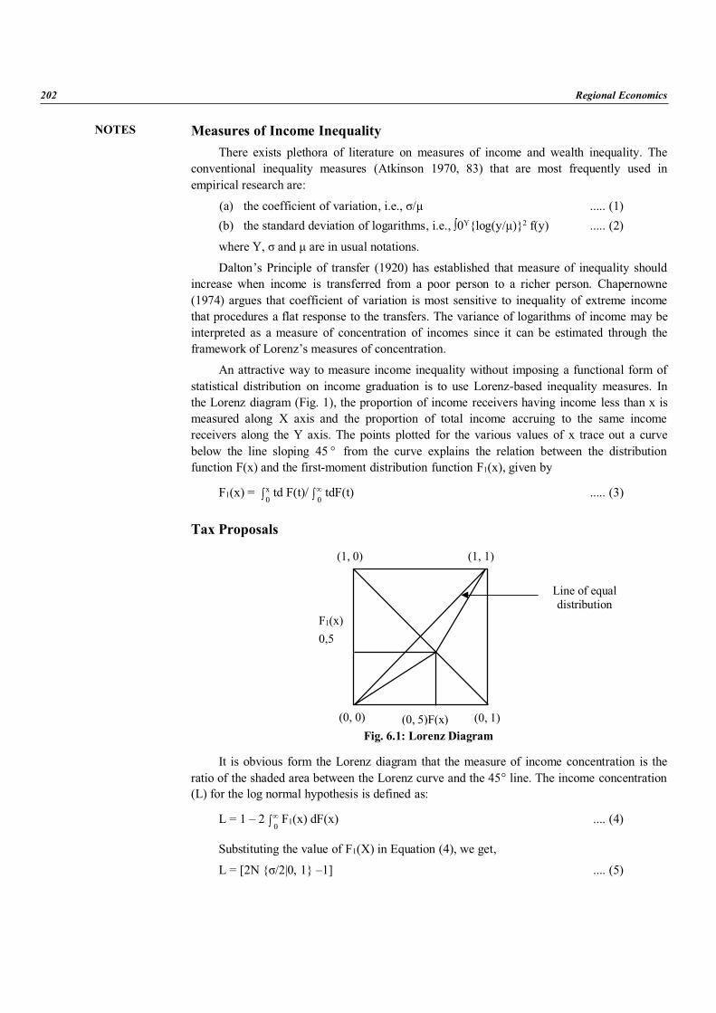
NOTES


Measures of Income InequalityThere exists plethora of literature on measures of income and wealth inequality. The

conventional inequality measures (Atkinson 1970, 83) that are most frequently used inempirical research are:

(a) the coefficient of variation, i.e., / ..... (1)(b) the standard deviation of logarithms, i.e., 0Y{log(y/ )}2 f(y) ..... (2)

where Y, and are in usual notations.

Dalton’s Principle of transfer (1920) has established that measure of inequality shouldincrease when income is transferred from a poor person to a richer person. Chapernowne(1974) argues that coefficient of variation is most sensitive to inequality of extreme incomethat procedures a flat response to the transfers. The variance of logarithms of income may beinterpreted as a measure of concentration of incomes since it can be estimated through theframework of Lorenz’s measures of concentration.

An attractive way to measure income inequality without imposing a functional form ofstatistical distribution on income graduation is to use Lorenz-based inequality measures. Inthe Lorenz diagram (Fig. 1), the proportion of income receivers having income less than x ismeasured along X axis and the proportion of total income accruing to the same incomereceivers along the Y axis. The points plotted for the various values of x trace out a curvebelow the line sloping 45 from the curve explains the relation between the distributionfunction F(x) and the first-moment distribution function F1(x), given by

F1(x) =0x td F(t)/

0tdF(t) ..... (3)

Tax Proposals

Fig. 6.1: Lorenz Diagram

It is obvious form the Lorenz diagram that the measure of income concentration is theratio of the shaded area between the Lorenz curve and the 45 line. The income concentration(L) for the log normal hypothesis is defined as:

L = 1 – 20

F1(x) dF(x) .... (4)

Substituting the value of F1(X) in Equation (4), we get,

L = [2N { /2|0, 1} –1] .... (5)

(1, 0) (1, 1)

F1(x)0,5

(0, 1)(0, 0) (0, 5)F(x)

Line of equaldistribution

NOTES


Obviously, the measure of concentration (L) is monotonically related to value of 2 andthus the parameter 2 (variance of logarithms of the income) may well be interpreted as ameasure of income inequality.

The Lorenz curve may again be generated by defining the income earner units, say,quintile shares where qi, i = 1, 2, ....., n reveals the share of ith income earner. Let, incomesare arranged in ascending order, i.e.,

0 q1 q2 ..... qi ..... qn 1 ..... (6)

From the order of the incomes as shown by Equation (6), several well-known incomeinequality measures may be derived. For example, the Gini (1912) measure of incomeinequality is given by the order of the incomes by Equation (6), several well-known

1– n

1 iiq i)– (n 2/n – 1/n – 1 G ..... (7)

and the relative mean deviationn

1 ii 1/n– q 1– n/n 1/2 R ..... (8)

On contrary, the Gini coefficient suffer with serious drawbacks, such as the simpleaging of a populations will raise income inequality. Gini coefficient is also insensitivity tonon-money components and differential price indices between states which exaggerateincome inequality in rural areas. The Gini ratio measures a property of distribution inequalitythat varies in direct proportion to the area of the closed geometric representation as shown inFig. 6.1.

Results and Interpretation: In order to study inter-state disparities in economic growth,total as well as per capita State Domestic Product (SDP) at current prices for the period 1980-2002 has been taken. State income are available from 1980-81 to 1998-99 at 1980-81 baseand later on it is available at 1993-94 base year. Thus, in order to evolve a comparable SDPwith a single base year, technique of base shifting has been applied for SDP data onwardsupto 1998-99 upto 2001-02 and SDP data for this period at base 1993-94 has been convertedat the base 1980-81 to prepare inter-state SDP from 1980-81 to 2001-02 at the base of1980- 81.

Average annual growth in total SDP for 1980-02 has been examined in the semi-logmodel with the help of slope-dummy and intercept-dummy technique with dummy variablefor year 1991, in order to detect any Kink, if any, in per annum growth in SDP around year1991, i.e., the period when economic reforms where introduced in India. Actually, per annumgrowth in total SDP has fallen for 20 states during reform period (1990-02). Disparity in totalSDP during this period has widen as per annum growth for relatively developed states likeGujarat (11.6 percent), Haryana (10.5 percent) and Maharashtra (10.9 percent) has beenfound higher than poor states like Bihar (7.4 percent), Madhya Pradesh (9.4 percent), Orissa(8.7 percent) and Uttar Pradesh (8.8 percent). Likewise, during reform period, per annumgrowth in total SDP were found lower for hill states as Assam (7.6 percent), HimachalPradesh (7.2 percent), Jammu & Kashmir (7.4 percent), Manipur (9.9 percent) and Tripura(7.8 percent) as compared to developed states like Gujarat, Haryana and Maharashtra.Widening economic disparities among states in terms of total as well as per capita SDP iscorroborated through enhancement in inequality indices over the period. Facts reveal thatGini index, RMD index, Theil’s index and Kakwani’s index for total SDP during 1980-81stood at 0.4409, 0.3372, 0.1147 and 0.1804 respectively and they remained almost stagnant

NOTES


upto 1990-91. But later on, these indices have risen and were recorded at 0.4558, 0.3459,0.1237 and 0.1929 respectively during 2001-02. Similarly, for per capita SDP, Gini index,RMD-index, Theil’s index and Kakwani’s index stood at 0.1493, 0.1177, 0.0124 and 0.0215respectively in 1980-81 and with mild enhancement these indices stood at 0.1596, 0.1164,0.0144 and 0.0248 respectively in 1990-91. Later on, a surge was found among theseinequality indices and finally these stood at 0.2171, 0.1660, 0.0249 and 0.0429 respectively in2001-02. Inequality indices pertaining to total as well as per capita SDP for 1980-2002 revealthe harsh inequalities at aggregate as well as per capita level have increased with is evident inincreasing values of inequality indices as mentioned above. These inequalities have beenmuch more prominent during the reform (1991-2002) period. Different measures ofconvergence/divergence, for instance -convergence and -convergence, have also beenestimated for the period 1980-2002 in order to examine the trends and issues pertaining tointer-state income disparities among twenty major Indian states. The estimated beta-coefficient are found positive and significant for all three periods, i.e., 1980-81 to 1990-91,1991-92 to 2001-02 and 1980-81 to 2001-02. Beta coefficients for reform period (1991-2002)as compared to pre-reform (1980-91) period suggest that economic reforms have resulted inwidening of inter-state disparities. As -coefficient for total as well as per capita SDP werefound negative (insignificant) during pre-reform (1980-1991) period indicating weakconvergence in state income during this period. However, Beta coefficient were foundpositive and significant for total as well as per capita SDP during reform (1991-2002) periodrevealing the fact that divergence in state income (total/per capita) resulting in increasinginter-state disparities has occurred after the reforms of 1991 have been introduced.

Thus, to conclude, the empirical results pertaining to interstate disparity in terms of totalas well as per capita for 20 major Indian states during the period 1980-2002 are quite patheticand alarming. Inequality indices for total SDP in terms of Gini ratio, RMD, Theil’s index andKakwani index stood at 0.4409, 0.3372, 0.1147 and 0.1804 respectively during 1980-81 andthese indices have risen, however moderately, and stood at 0.4558, 0.3459, 0.1237 and0.1929 respectively in 2001-02. These indices for per capita SDP were noted at 0.1493,0.1177, 0.0124 and 0.0215 respectively during 1980-81 and these indices have risen drasticallylater on and were observed at 0.2171, 0.1660, 0.0249 and 0.0429 in the year 2001-02.Widening gap in terms of income among rich and poor states, especially after 1991 has alsobeen established through empirical results based on -convergence and -convergence. Thisis indeed an alarming situation and a potential threat for stability of a federation like India.Redressal of horizontal economic disparity happens to be an important objective in anyscheme of federal devolution of funds among federating states.In India, this task is done bythe Planning Commission and Finance Commission. The Thirteenth Finance Commission(2010-15) should assign due weight age to this factor in its scheme of devolution of taxes orgrants for states such that inter-state economic disparities may be rectified effectively.

6.4 FISCAL PROGRAMMES

Fiscal policy deals with the taxation and expenditure decisions of the government.Monetary policy deals with the supply of money in the economy and the rate of interest.These are the main policy approaches used by economic managers to steer the broad aspectsof the economy. In most modern economies, the government deals with fiscal policy whilethe central bank is responsible for monetary policy. Fiscal policy is composed of several parts.These include tax policy, expenditure policy, investment or disinvestment strategies and debtor surplus management. Fiscal policy is an important constituent of the overall economic

NOTES


framework of a country and is therefore intimately linked with its general economic policystrategy.

Fiscal policy also feeds into economic trends and influences monetary policy. When thegovernment receives more than it spends, it has a surplus. If the government spends morethan it receives, it runs a deficit. To meet the additional expenditures, it needs to borrow fromdomestic or foreign sources, draw upon its foreign exchange reserves or print an equivalentamount of money. This tends to influence other economic variables. On a broadgeneralization, excessive printing of money leads to inflation. If the government borrows toomuch from abroad, it leads to a debt crisis. If it draws down on its foreign exchange reserves,a balance of payments crisis may arise. Excessive domestic borrowing by the governmentmay lead to higher real interest rates and the domestic private sector being unable to accessfunds resulting in the crowding out of private investment. Sometimes, a combination of thesecan occur. In any case, the impact of a large deficit on long-run growth and economic well-being is negative. Therefore, there is broad agreement that it is not prudent for a governmentto run an unduly large deficit. However, in case of developing countries, where the need forinfrastructure and social investments may be substantial, it sometimes argued that runningsurpluses at the cost of long-term growth might also not be wise. The challenge then for mostdeveloping country governments is to meet infrastructure and social needs while managingthe government’s finances in a way that the deficit or the accumulating debt burden is not toogreat.

Here, we shall study the trajectory of India’s fiscal policy with particular focus onhistorical trends, the development of fiscal discipline frameworks, the recent experience offiscal response to the global financial crisis and subsequent return to a fiscal consolidationpath. The initial years of India’s planned development strategy were characterized by aconservative fiscal policy whereby deficits were kept under control. The tax system wasgeared to transfer resources from the private sector to fund the large public sector drivenindustrialization process and also cover social welfare schemes. Indirect taxes were a largersource of revenue than direct taxes. However, growth was anaemic and the system was proneto inefficiencies. In the 1980s, some attempts were made to reform particular sectors andmake some changes in the tax system. But the public debt increased, as did the fiscal deficit.Triggered by higher oil prices and political uncertainties, the balance of payments crisis of1991 led to economic liberalization. The reform of the tax system commenced with directtaxes increasing their share in comparison to indirect taxes. The fiscal deficit was broughtunder control. When the deficit and debt situation again threatened to go out of control in theearly 2000s, fiscal discipline legalizations were instituted at the central level and in moststates. The deficit was brought under control and by 2007-08 a benign macro-fiscal situationwith high growth and moderate inflation prevailed. The global financial crisis tested the fiscalpolicy framework and it responded with counter-cyclical measures including tax cuts andincreases in expenditures. The post-crisis recovery of the Indian economy is witnessing acorrection of the fiscal policy path towards a regime of prudence. In the future, the focuswould probably be on bringing in new tax reforms and better targeting of social expenditures.

Basic ConceptsAt the outset, it is important to clarify certain basic concepts. The most elementary is

perhaps the difference between revenue and capital flows, be they receipts or expenditures.While there are various complex legal and formal definitions for these ideas, presenting somesimplified and stylized conceptual clarifications is deemed appropriate. A spending item is acapital expenditure if it relates to the creation of an asset that is likely to last for a

NOTES


considerable period of time and includes loan disbursements. Such expenditures are generallynot routine in nature. By the same logic, a capital receipt arises from the liquidation of anasset including the sale of government shares in public sector companies (disinvestments), thereturn of funds given on loan or the receipt of a loan. This again usually arises from acomparatively irregular event and is not routine. In contrast, revenue expenditures are fairlyregular and generally intended to meet certain routine requirements like salaries, pensions,subsidies, interest payments, and the like. Revenue receipts represent regular earnings, forinstance, tax receipts and non-tax revenues including from sale of telecom spectrums.

There are various ways to represent and interpret a government’s deficit. The simplest isthe revenue deficit which is just the difference between revenue receipts and revenueexpenditures.

Revenue Deficit = Revenue Expenditure – Revenue Receipts (i.e., Tax + Non-taxRevenue)

A more comprehensive indicator of the government’s deficit is the fiscal deficit. This isthe sum of revenue and capital expenditure less all revenue and capital receipts other thanloans taken. This gives a more holistic view of the government’s funding situation since itgives the difference between all receipts and expenditures other than loans taken to meet suchexpenditures.

Fiscal Deficit = Total Expenditure (i.e., Revenue Expenditure + Capital Expenditure) –(Revenue Receipts + Recoveries of Loans + Other Capital Receipts (i.e., all Revenue andCapital Receipts other than loans taken))

The gross fiscal deficit (GFD) of government is the excess of its total expenditure,current and capital, including loans net of recovery, over revenue receipts (including externalgrants) and non-debt capital receipts. The net fiscal deficit is the gross fiscal deficit reducedby net lending by government. The gross primary deficit is the GFD less interest paymentswhile the primary revenue deficit is the revenue deficit less interest payments.

India’s Fiscal Policy ArchitectureThe Indian Constitution provides the overarching framework for the country’s fiscal

policy. India has a federal form of government with taxing powers and spendingresponsibilities being divided between the Central and the State Governments according tothe Constitution. There is also a third tier of government at the local level. Since the taxingabilities of the states are not necessarily commensurate with their spending responsibilities,some of the centre’s revenues need to be assigned to the state governments. To provide thebasis for this assignment and give medium term guidance on fiscal matters, the Constitutionprovides for the formation of a Finance Commission (FC) every five years. Based on thereport of the FC, the central taxes are devolved to the state governments. The Constitutionalso provides that for every financial year, the government shall place before the legislature astatement of its proposed taxing and spending provisions for legislative debate and approval.This is referred to as the Budget. The central and the state governments each have their ownbudgets.

The central government is responsible for issues that usually concern the country as awhole like national defence, foreign policy, railways, national highways, shipping, airways,post and telegraphs, foreign trade and banking. The state governments are responsible forother items including, law and order, agriculture, fisheries, water supply and irrigation, andpublic health. Some items for which responsibility vests in both the Centre and the States

NOTES


include forests, economic and social planning, education, trade unions and industrial disputes,price control and electricity. There is now increasing devolution of some powers to localgovernments at the city, town and village levels. The taxing powers of the central governmentencompass taxes on income (except agricultural income), excise on goods produced (otherthan alcohol), customs duties, and inter-state sale of goods. The state governments are vestedwith the power to tax agricultural income, land and buildings, sale of goods (other than inter-state), and excise on alcohol.

Besides the annual budgetary process, since 1950, India has followed a system of fiveyear plans for ensuring long-term economic objectives. This process is steered by thePlanning Commission for which there is no specific provision in the Constitution. The mainfiscal impact of the planning process is the division of expenditures into plan and non-plancomponents. The plan components relate to items dealing with long-term socio-economicgoals as determined by the ongoing plan process. They often relate to specific schemes andprojects. Furthermore, they are usually routed through central ministries to state governmentsfor achieving certain desired objectives. These funds are generally in addition to theassignment of central taxes as determined by the Finance Commissions. In some cases, thestate governments also contribute their own funds to the schemes. Non-plan expendituresbroadly relate to routine expenditures of the government for administration, salaries, and thelike.

While these institutional arrangements initially appeared adequate for driving thedevelopment agenda, the sharp deterioration of the fiscal situation in the 1980s resulted in thebalance of payments crisis of 1991, which would be discussed later. Following economicliberalization in 1991, when the fiscal deficit and debt situation again seemed to head towardsunsustainable levels around 2000, a new fiscal discipline framework was instituted. At thecentral level, this framework was initiated in 2003 when the Parliament passed the FiscalResponsibility and Budget Management Act (FRBMA).

Taxes are the main source of government revenues. Direct taxes are so named sincethey are charged upon and collected directly from the person or organization that ultimatelypays the tax (in a legal sense). Taxes on personal and corporate incomes, personal wealth andprofessions are direct taxes. In India, the main direct taxes at the central level are the personaland corporate income tax. Both are till date levied through the same piece of legislation, theIncome Tax Act of 1961. Income taxes are levied on various heads of income, namely,incomes from business and professions, salaries, house property, capital gains and othersources (like interest and dividends). Other direct taxes include the wealth tax and thesecurities transactions tax. Some other forms of direct taxation that existed in India from timeto time but were removed as part of various reforms include the estate duty, gift tax,expenditure tax and fringe benefits tax. The estate duty was levied on the estate of a deceasedperson. The fringe benefits tax was charged on employers on the value of in-kind non-cashbenefits or perquisites received by employees from their employers. Such perquisites are nowlargely taxed directly in the hands of employees and added to their personal income tax.Some states charge a tax on professions. Most local governments also charge property ownersa tax on land and buildings.

Indirect taxes are charged and collected from persons other than those who finally endup paying the tax. For instance, a tax on sale of goods is collected by the seller from the buyer.The legal responsibility of paying the tax to government lies with the seller, but the tax ispaid by the buyer. The current central level indirect taxes are the central excise (a tax onmanufactured goods), the service tax, the customs duty (a tax on imports) and the central

NOTES


sales tax on inter-state sale of goods. The main state level indirect tax is the post-manufacturing (that is wholesale and retail levels) sales tax (now largely a value added taxwith intra-state tax credit). The complications and economic inefficiencies of this multiplecascading taxation across the economic value chain (necessitated by the constitutionalassignment of taxing powers) are discussed later in the context of the proposed Goods andServices Tax (GST).

Evolution of Indian Fiscal Policy till 1991India commenced on the path of planned development with the setting up of the

Planning Commission in 1950. That was also the year when the country adopted a FederalConstitution with strong unitary features giving the central government primacy in terms ofplanning for economic development. The subsequent planning process laid emphasis onstrengthening public sector enterprises as a means to achieve economic growth and industrialdevelopment. The resulting economic framework imposed administrative controls on variousindustries and a system of licensing and quotas for private industries. Consequently, the mainrole of fiscal policy was to transfer private savings to cater to the growing consumption andinvestment needs of the public sector. Other goals included the reduction of income andwealth inequalities through taxes and transfers, encouraging balanced regional development,fostering small-scale industries and sometimes influencing the trends in economic activitiestowards desired goals.

In terms of tax policy, this meant that both direct and indirect taxes were focussed onextracting revenues from the private sector to fund the public sector and achieveredistributive goals. The combined centre and state tax revenue to GDP ratio increased from6.3 percent in 1950-51 to 16.1 percent in 1987-88. For the central government, this ratio was4.1 percent of GDP in 1950-51 with the larger share coming from indirect taxes at 2.3 percentof GDP and direct taxes at 1.8 percent of GDP. Given their low direct tax levers, the stateshad 0.6 percent of GDP as direct taxes and 1.7 percent of GDP as indirect taxes in 1950-51.

The government authorized a comprehensive review of the tax system culminating inthe Taxation Enquiry Commission Report of 1953. However, the government then invited theBritish economist Nicholas Kaldor to examine the possibility of reforming the tax system.Kaldor found the system inefficient and inequitable given the narrow tax base and inadequatereporting of property income and taxation. He also found the maximum marginal income taxrate at 92 percent to be too high and suggested it be reduced to 45 percent. In view of hisrecommendations, the government revived capital gains taxation, brought in a gift tax, awealth tax and an expenditure tax (which was not continued due to administrativecomplexities).

Despite Kaldor’s recommendations, income and corporate taxes at the highest marginalrate continued to be extraordinarily high. In 1973-74, the maximum rate taking into accountthe surcharge was 97.5 percent for personal income above ` 0.2 million. The system was alsocomplex with as many as eleven tax brackets. The corporate income tax was differential forwidely held and closely held companies with the tax rate varying from 45 to 65 percent forsome widely held companies. Though the statutory tax rates were high, given a large numberof special allowances and depreciation, effective tax rates were much lower. The DirectTaxes Enquiry Committee of 1971 found that the high tax rates encouraged tax evasion.Following its recommendations in 1974-75, the personal income tax rate was brought downto 77 percent but the wealth tax rate was increased. The next major simplification was in

NOTES


1985-86 when the number of tax brackets was reduced from eight to four and the highestincome tax rate was brought down to 50 percent.

In indirect taxes, a major component was the central excise duty. This was initially usedto tax raw materials and intermediate goods and not final consumer goods. But by 1975-76, itwas extended to cover all manufactured goods. The excise duty structure at this time wascomplicated and tended to distort economic decisions. Some commodities had specific dutieswhile others had ad valorem rates. The tax also had a major cascading effect since it wasimposed not just on final consumer goods but also on inputs and capital goods. In effect, thetax on the input was again taxed at the next point of manufacture resulting in double taxationof the input. Considering that the states were separately imposing sales tax at the post-manufacturing wholesale and retail levels, this cascading impact was considerable. TheIndirect Tax Enquiry Report of 1977 recommended introduction of input tax credits toconvert the cascading manufacturing tax into a manufacturing value added tax (MANVAT).Instead, the modified value added tax (MODVAT) was introduced in a phased manner from1986 covering only selected commodities.

The other main central indirect tax is the customs duty. Given that imports into Indiawere restricted, this was not a very large source of revenue. The tariffs were high anddifferentiated. Items at later stages of production like finished goods were taxed at higherrates than those at earlier stages, like raw materials. Rates also differed on the basis ofperceived income elasticities with necessities taxed at lower rates than luxury goods.In 1985-86, the government presented its Long-term Fiscal Policy stressing on the need toreduce tariffs, have fewer rates and eventually remove quantitative limits on imports. Somereforms were attempted but due to revenue raising considerations, the tariffs in terms of theweighted average rate increased from 38 percent in 1980-81 to 87 percent in 1989-90. By1990-91, the tariff structure had a range of 0 to 400 percent with over 10 percent of importssubjected to tariffs of 120 percent or more. Further complications arose from exemptionsgranted outside the budgetary process.

In 1970-71, direct taxes contributed to around 16 percent of the central government’srevenues, indirect taxes about 58 percent and the remaining 26 percent came from non-taxrevenues. By 1990-91, the share of indirect taxes had increased to 65 percent, direct taxesshrank to 13 percent and non-tax revenues were at 22 percent. India’s expenditure normsremained conservative till the 1980s. From 1973-74 to 1978-79 the central governmentcontinuously ran revenue surpluses. Its gross fiscal deficit also showed a slow growth withcertain episodes of downward movements. The state governments also ran revenue surplusesfrom 1974-75 to 1986-87, barring only 1984-85. Thereafter, limited reforms in specific areasincluding trade liberalization, export promotion and investment in modern technologies wereaccompanied by increased expenditures financed by domestic and foreign borrowings. Thecentral revenue deficit climbed from 1.4 percent of GDP in 1980-81 to 2.44 percent of GDPby 1989-90. Across the same period, the centre’s gross fiscal deficit (GFD) climbed from5.71 percent to 7.31 percent of GDP. Though the external liabilities of the centre fell from7.16 percent of GDP in 1982-83 to 5.53 percent of GDP by 1990-91, in absolute terms, theliabilities were large. Across the same period, the total liabilities of the centre and the statesincreased from 51.43 percent of GDP to 64.75 percent of GDP.

This came at the cost of social and capital expenditures. The interest component ofaggregate central and state government disbursements reflects this quite clearly. The capitaldisbursements decreased from around 30 percent in 1980-81 to about 20 percent by 1990-91.In contrast, the interest component increased from around 8 percent to about 15 percent

NOTES


across the same period. Within revenue expenditures, in 1970-71, defence expenditures hadthe highest share of 34 percent, interest component was 19 percent while subsidies were only3 percent. However, by 1990-91, the largest component was the interest share of 29 percentwith subsidies constituting 17 percent and defence only 15 percent. Therefore, besides theburden of servicing the public debt, the subsidy burden was also quite great.

While India’s external debt and expenditure patterns were heading for unsustainablelevels, the proximate causes of the balance of payments crisis came from certain unforeseenexternal and domestic political events. The First Gulf War caused a spike in oil prices leadingto a sharp increase in the government’s fuel subsidy burden. Furthermore, the assassination offormer Prime Minister Rajiv Gandhi increased political uncertainties leading to thewithdrawal of some foreign funds. The subsequent economic reforms changed the Indianeconomy forever.

Liberalization, Growth, Inclusion and Fiscal Consolidation (1991-2008)Following the balance of payments crisis of 1991, the government commenced on a

path of economic liberalization whereby the economy was opened up to foreign investmentand trade, the private sector was encouraged and the system of quotas and licences wasdismantled. Fiscal policy was reoriented to cohere with these changes.

The Tax Reforms Committee provided a blueprint for reforming both direct and indirecttaxes. Its main strategy was to reduce the proportion of trade taxes in total tax revenue,increase the share of domestic consumption taxes by converting the excise into a VAT andenhance the contribution of direct taxes to total revenue. It recommended reducing the ratesof all major taxes, minimizing exemptions and deductions, simplifying laws and procedures,improving tax administration and increasing computerization and information systemmodernization.

As a part of the subsequent direct tax reforms, the personal income tax brackets werereduced to three with rates of 20, 30 and 40 percent in 1992-93. Financial assets wereremoved from the imposition of wealth tax and the maximum rate of wealth tax was reducedto 1 percent. Personal income tax rates were reduced again to 10, 20, and 30 percent in 1997-98. The rates have largely remained the same since with the exemption limit being increasedand slab structure raised from time to time. A subsequent 2 percent surcharge to fundeducation was later made applicable to all taxes. The basic corporate tax rate was reduced to50 percent and the rates for different closely held companies made uniform at 55 percent. In1993-94, the distinction between the closely held and the widely held companies wasremoved and the uniform tax rate was brought down to 40 percent. The rate was furtherreduced to 35 percent with a 10 percent tax on distributed dividends in 1997-98.

Despite these reforms, the tax system continued to have preferential exemptions anddeductions as tax incentives for various socio-economic goals including location of industriesin backward areas, export promotion and technology development. This led to thephenomenon of zero-tax companies whereby imaginative arrangements were use to leverageall these tax incentives with an intent to minimize tax liabilities. To counter this trend, theMinimum Alternative Tax (MAT) was introduced in 1996-97. It required a company to pay aminimum of 30 percent of book profits as tax. Further attempts to expand the tax base andincrease revenues were the introduction of the securities transaction tax (STT) in 2004 andthe fringe benefit tax (FBT) in the budget of 2005-06.

In indirect taxes, the MODVAT credit system for excise was expanded to cover mostcommodities and provide a comprehensive credit system by 1996-97. The eleven rates were

NOTES


merged into three with a few luxury items subject to additional non-rebatable tax in1999-2000. In 2000-01, the three rates were merged in to a single rate and renamed as centralVAT (CENVAT). There remained three additional excises of 8, 16 and 24 percent. In case ofcustom duties, in 1991-92, all duties on non-agriculture goods that were above 150 percentwere brought down to this rate. The peak rate was brought down to 40 percent in 1997-98,30 percent in 2002-03, 25 percent in 2003-04, and 15 percent in 2005-06. The number ofmajor duty rates was also brought down from 22 in 1990-91 to 4 in 2003-04. These four ratescovered almost 90 percent of customs collected from items. This period also saw theintroduction of the service tax in 1994-95, which was subsequently expanded to cover moreand more services. Given that the Indian economy was having an increasingly large servicecomponent, this increasingly became a major source of revenue. Eventually, provisions weremade for allowing input tax credits for both goods and services at the central indirect taxlevel.

Despite the reforms in central taxes, even after the economic reforms of 1991, stategovernment tax reforms were inadequate and sporadic. A major move in this direction wasthe co-ordinated simplification of the state sales tax system in 1999. This eventually led to theintroduction of a VAT in 21 states in 2005. The value added tax gives credit to taxes paid oninputs and provides relief from cascading. Implemented at the retail level, this replaced thecascading sales tax providing great relief to consumers and traders alike while enhancing therevenues of the state government. The administrative design of the VAT ensures reporting ofinputs and outputs resulting in substantial reduction in tax evasion. The basic features of thetax include two rates of 4 percent for common consumption commodities and inputs and12.5 percent for the others. Some essential items are exempted and precious metals are taxedat 1 percent. The credit system covers inputs and purchases as also capital goods formanufacturers as well as dealers. Credit for capital goods taxes can be availed over threeyears of sales. The tax credit operates fully only for intra-state sales. This is a majorhindrance to the formation of a smooth nationwide market and is to be addressed by theproposed Goods and Services Tax (GST).

In consonance with the tax reform plans, the sources of central government revenueshifted from indirect taxes towards direct taxes. In 1995-96, about 54 percent of revenuescame from indirect taxes while around 20 percent were from direct taxes. In 2000-01, theshare of indirect taxes had gone down dramatically to around 45 percent while thecontribution from direct taxes had increased to about 26 percent. By 2005-06, indirect taxesaccounted for approximately 43 percent while the direct taxes share was about 35 percent.The post-1991 expenditure strategy focussed on reducing subsidies and cutting down on non-capital expenditures. However, the large debt burden meant that the interest componentwould take a long time to ebb. In 1995-96, of the central government’s revenue expenditures,9 percent went to subsidies, 13 percent to defence and 36 percent to interest.

Five years later in 2000-01, defence and interest remained at 13 percent and 36 percent,respectively, while subsidies increased slightly to 10 percent. This reveals that thecomposition of government expenditure generally does not change very fast. By 2005-06, theinterest component had come down to 30 percent and defence and subsidies each took up11 percent. As a component of aggregate disbursements of the central and state governments,the interest component continued to rise till around 2002-03 and then started to decline.Capital disbursements showed just the opposite trend falling till around 2002-03 and thenrising till 2007-08.

NOTES


The rising revenues from tax administration reforms and expenditure control resulted inthe deficits being brought under control. The central government’s revenue deficit went downto 2.37 percent of GDP in 1996-97 while the GFD was 4.84 percent. The government wasalso more prudent about its external debt. The debt to GDP ratio went down to 4.3 percent ofGDP in 1995-96 and reached a further low point of 2.99 percent in 1999-00. However,government debt and fiscal discipline again seemed to give way in the early 2000s. Thecentral government’s revenue deficit climbed up to 4.4 percent of GDP in 2002-03 while theGFD was at 5.91 percent of GDP. By 2003-04, the combined liabilities of the centre and thestates were up at 81.09 percent of GDP from 70.59 percent in 2000-01. The externalliabilities were, however, kept under control at only 1.67 percent of GDP in 2003-04.

It was obvious that a new fiscal discipline framework was urgently required. Afteraround three years of discussions, the FRBMA was adopted in 2003. This Act gave amedium-term target for balancing current revenues and expenditures and set overall limits tothe fiscal deficit at 3 percent of GDP to be achieved according to a phased deficit reductionroadmap. The FRBMA enhanced budgetary transparency by requiring the government toplace before the Parliament on an annual basis reports related to its economic assessments,taxation and expenditure strategy and three-year rolling targets for the revenue and fiscalbalance. It also required quarterly progress reviews to be placed in Parliament. A largenumber of state governments also brought out their own fiscal discipline legislations.

These fiscal discipline legislations seemed to have had good impact at both the centraland state levels. The year before the global financial crisis in 2007-08, the centralgovernment’s revenue deficit came down to 1.06 percent of GDP while the GFD was3.33 percent. The state governments achieved a revenue surplus of 0.58 percent of GDP and aGFD of 1.81 percent of GDP by 2006-07. Even in the year of the crisis, in 2008-09, they hada small revenue surplus of 0.19 percent of GDP and a GFD of 3.2 percent of GDP. This fiscaldiscipline fed into other economic variables in a positive manner. The aggregatedisbursements of the central and state governments showed an increase in capital outlaysfrom 11.87 percent in 2002-03 to 18.59 percent in 2007-08. Inflation was moderate andgrowth was buoyant at 9.6 percent in 2006-07. This benign macroeconomic environment wasdisturbed by the global financial crisis.

Crisis and Return to Fiscal Consolidation: The Maturing of Indian FiscalPolicy

The global financial crisis that erupted around September 2008 saw Indian fiscal policybeing tested to its limits. The policy makers had to grapple with the impact of the crisis thatwas affecting the Indian economy through three channels: contagion risks to the financialsector; the negative impact on exports; and the effect on exchange rates. Somewhatserendipitously, the government already had an expansionary fiscal stance in view of a ruralfarm loan waiver scheme, the expansion of social security schemes under the National RuralEmployment Guarantee Act (NREGA) and the implementation of revised salaries andcompensations for the central public servants as per the recommendations of the Sixth PayCommission. Furthermore, the parliamentary elections of 2008 also resulted in furthergovernment expenditures.

As the crisis unfolded, the government activated a series of stimulus packages on7th December 2008, 2nd January 2009 and 24th February 2009. Actions included an overallcentral excise duty cut of 4 percent, ramping up additional plan expenditure of about ` 200billion, further state government borrowings for planned expenditure amounting to around

NOTES


` 300 billion, interest subsidies for export finance to support certain export oriented industries,a further 2 percent reduction of central excise duties and service tax for export industries (thatis a total 6 percent central excise reduction). The impact of these measures is estimated to bearound 1.8 percent of GDP in 2008-09. If the increase in public expenditure across thebudgets of 2007-08 and 2008-09 is taken together, it amounted to about 3 percent of GDP.

Given its inherent strengths like a strong and prudently regulated financial sector, a wellmanaged capital account policy, large foreign exchange reserves, strong domesticconsumption and effective fiscal policy interventions, the Indian economy weathered thefinancial crisis rather well. GDP growth declined to 5.8 percent (year-on-year) in the secondhalf of 2008-09 compared to 7.8 percent in the first half. By 2009-10, India’s GDP wasgrowing at 8 percent (quick estimates (QE)). This increased to 8.5 percent in 2010-11(revised estimates (RE)).

It was now important that the process of fiscal consolidation be reinstated. This was adelicate process where the fiscal tightening had to be achieved without prematurely chokingoff the growth process. The Thirteenth Finance Commission (13th FC) in its report waskeenly conscious of the need to return to the path of fiscal prudence and provided a road mapcharting a set of desired fiscal deficit targets. The budget of 2010-11 adopted a calibrated exitpolicy targeting a fiscal deficit of 5.5 percent of GDP in 2010-11 from a level of 6.5 percent(inclusive of bonds in lieu of securities) in 2009-10 (Ministry of Finance, 2011).

In course of 2010-11, the non-tax revenues from auction of telecom spectrum (3G andbroadband) resulted in higher than anticipated receipts. A conscious decision was taken toincrease allocation to priority sectors while adhering to the fiscal deficit target. Ultimately,the fiscal deficit for 2010-11 declined to a better than targeted 5.1 percent of GDP. This wasalso an improvement over the 13th FC roadmap target of 5.7 percent. The government’smedium-term fiscal policy statement as mandated by the FRBMA for the annual Budget2011-12 projected continuing on a path of gradual adjustment at a pace faster than thatprescribed by the 13th FC. The 2011-12 fiscal deficit target was set at 4.6 percent of GDP asagainst the 13th FC target of 4.8 percent. The rationale for this was that reducing the debt toGDP ratio at an accelerated pace would unlock more resources for use in developmentalprogrammes instead of debt servicing (Ministry of Finance, 2011).

By 2009-10, direct taxes were contributing around 48 percent of revenues while theindirect taxes share was about 32 percent. In the Budget of 2011-12, the share of direct taxeswas about 47 percent of the central government’s projected revenue while the indirect taxescontribution was around 37 percent. The move to increase the share of direct taxes asenvisaged in 1991 had therefore been achieved.

In terms of tax policy, after the conscious slackening of the tax to GDP ratio in the wakeof the crisis, a tightening was seen to be desirable. The Budget of 2011-12 aimed atdovetailing both direct and indirect tax policy with medium-term objectives of fiscalconsolidation and the proposed adoption of major new tax legislations; the Direct Tax Code(DTC) for direct taxes and the Goods and Services Tax (GST) in case of indirect taxes. Inindirect taxes, among major proposals, the central excise merit rate was increased from4 percent to 5 percent, branded ready made garments were subjected to excise duty of10 percent, and few additional services were brought in under the service tax net. In the caseof direct taxes, the personal income tax exemption limit was increased. and the surcharge oncorporate income tax for domestic companies was reduced from 7.5 percent to 5 percentresulting in the overall rate coming down from 33.2 percent to 32.4 percent. Certain changes

NOTES


were also made to the Minimum Alternate Tax (MAT) provisions to maintain revenueneutrality and preserve horizontal equity as far as possible.

The government’s expenditure management initiatives also seemed to have gatheredmomentum with a focus on outcomes rather than allocations. For this, select departments aremandated to develop their Result Framework Document with an emphasis on trackingmeasurable outcomes. In 2009-10, defence expenditures made up around 10 percent,subsidies 16 percent and interest 23 percent of revenue expenditures. The situation remainedmore or less the same in the Budget of 2011-12, revealing once again the largely slowchanging nature of the composition of government expenditures. Of the government’sprojected revenue expenditures for 2011-12, defence constitutes 9 percent, subsidies13 percent and interest 24 percent.

It now appears that fiscal prudence and the desire to limit the public debt through betterrevenue and expenditure outcomes has been fairly institutionalized in the Indian policymatrix. This is probably partly attributable to the anchoring role played by the FRBMA andthe deficit reduction roadmaps put forward by the 13th Finance Commission. Despite thetemporary deviation from stringent fiscal consolidation targets necessitated by the globalfinancial crisis, Indian fiscal policy is being steered rapidly back to the path of prudence. Thedetermination displayed by policy makers to set for themselves strict deficit reduction targets,often exceeding those mandated by the 13th FC appear to demonstrate that fiscal discipline ishere to stay.

Recent developments indicate that policy makers have come to accept strict budgetaryconstraints, while attempting to maximize resources for developmental activities. ThePlanning Commission abundantly reveals this in its preparatory reports for the 12th Five YearPlan (2012-17). The approach paper to the plan while projecting the centre’s fiscal resourcesassiduously envisages an average fiscal deficit of 3.25 percent of GDP for the entire planperiod with the fiscal deficit projected to come down from 4.1 percent in 2012-13 to3.5 percent in 2013-14. It is then expected to remain at 3 percent of GDP for the next threefinancial years. The gross budgetary support for the plan is kept realistic. It is projected toincrease from 4.92 percent of GDP in 2011-12 to 5.75 percent by the end of the 12th Plan.Similarly, revenue targets are projected at conservative levels. Net tax revenue for the centreis expected to increase from 7.4 percent of GDP in 2011-12 to 8.91 percent in 2016-17. Thegross tax to GDP ratio is projected to be 10.36 percent of GDP in 2011-12 rising to12.3 percent by 2016-17. This is somewhat optimistic given that this ratio previously peakedat 11.9 percent in 2007-08. It appears that the planners are relying on critical tax reforms,especially the GST to deliver the much-needed revenue boost. Since chances of large non-taxrevenues like spectrum auctions are unlikely, such revenues are expected to fall from1.4 percent of GDP in 2011-12 to 0.88 percent of GDP in 2016-17. Similarly, non-debtcapital receipts (mainly proceeds from disinvestment) are expected to fall (PlanningCommission, 2011).

Rather than rely on revenue performance alone, expenditure reforms with effectivetargeting of subsidies appears to be a major policy strategy. For the 12th Plan with regard tonon-plan expenditure, defence expenditure is projected to fall from 1.83 percent of GDP inthe base year (2011-12) to 1.56 percent in the final year (2016-17). Subsidies are forecast todecline from 1.6 percent of GDP in 2011-12 to 1.24 percent of GDP in 2016-17. They wouldstill account for 18.8 percent of total projected non-plan expenditure during the 12th Plan.The ability to control subsidies would hinge critically on global oil prices and the success ofplanned measures to target subsidies through improved delivery mechanisms. While the

NOTES


former is beyond the control of policy makers, the latter would then be a key focus area(Planning Commission, 2011). Looking ahead, the government would probably focus onreforms on both the tax and expenditure fronts. With regard to tax policy, changes can beexpected in terms of legislation as well as administrative reforms to improve efficiency. Themain legislative proposals are the DTC and the GST both of which are in various stages oflegislative consultation. The DTC seeks to simplify the tax code, revamp the system of taxdeductions and remove ambiguities of law. The GST aims at bringing a fairly unified systemof input tax credits across the value chain and at an inter-state level. Currently, the centralexcise and service taxes have limited credit facilities up to the manufacturing stage. The stateVAT is not geared to provide inter-state input tax credits. It is proposed to institute a dualGST structure with separate central and state GSTs. This would require a constitutionalamendment to allow both the central and state governments to have concurrent jurisdictionover the entire value chain. Inter-state GST credit and full credit for the central GST isenvisaged. This would also require an advanced information technology (IT) infrastructure(Empowered Committee, 2009). It is also likely to be further leveraged for improving thedirect tax administration. Moves in this direction include increasing the number ofCentralized Processing Centres (CPCs) that carry out bulk processing functions from one tofour. The number of taxpayer help centres and web-based taxpayer interface facilities are alsoto be increased substantially (Ministry of Finance, 2011).

It also appears that there are moves to improve social expenditure outcomes and targetsubsidies in a better manner. With respect to energy related subsidies in particular, given theIntegrated Energy Policy of 2009, the basic principle would be to equalize the prices ofdomestic energy with that of imported energy while targeting subsidies to the poor and needy(Planning Commission, 2011). Much of this would hinge on the adoption of new techniquesand technologies including IT based identification systems as proposed by the Aadhar UniqueIdentification system.

Thus, to sum up, it is found that the major developments in India’s fiscal policy fromthe early stages of planned development in the 1950s, through the country’s balance ofpayments crisis of 1991, the subsequent economic liberalization and rapid growth phase, theresponse to the global financial crisis of 2008 and the recent post-crisis moves to return to apath of fiscal consolidation. India’s fiscal policy in the phase of planned developmentcommencing from the 1950s to economic liberalization in 1991 was largely characterized bya strategy of using the tax system to transfer private resources to the massive investments inthe public sector industries and also achieve greater income equality. The result was highmaximum marginal income tax rates and the consequent tendency of tax evasion. The publicsector investments and social expenditures were also not efficient. Given these apparentinadequacies, there were limited attempts to reform the system in the 1980s. However, thepath of debt-induced growth that was pursued partly contributed to the balance of paymentscrisis of 1991.

Following the crisis of 1991, the government charted out a path of economicliberalization. Tax reforms focussed on lowering of rates and broadening of the tax base.There were attempts to curb subsidies and disinvest the government holdings in the publicsector industries. While initially the fiscal deficit and public debt were brought under control,the situation again started to deteriorate in the early 2000s. This induced the adoption of fiscalresponsibility legislations at the central and state levels. There were also reforms in the statelevel tax system with the introduction of VAT. Consequently, there were majorimprovements in the public finances. This probably contributed to the benign macro-fiscalenvironment of high growth, low deficits and moderate inflation that prevailed around 2008.

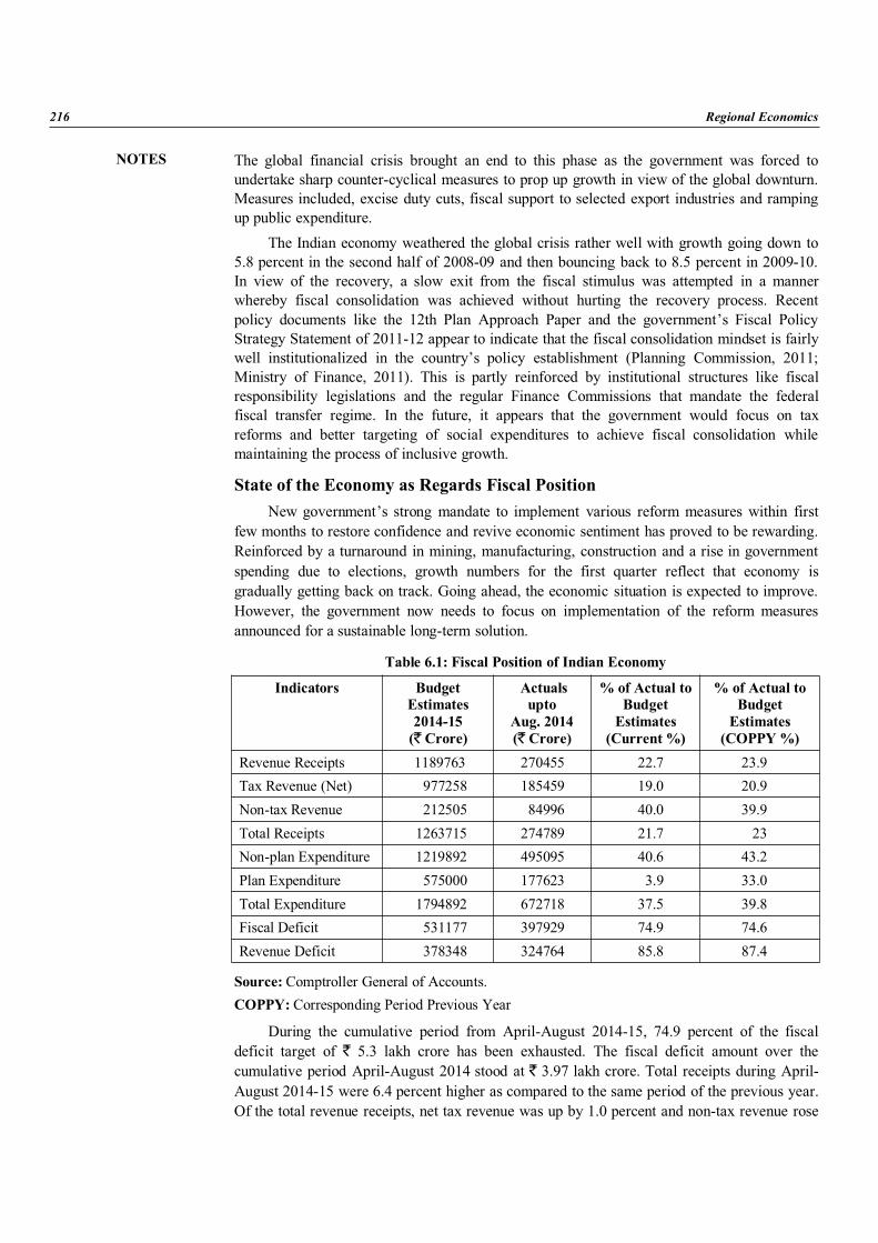
NOTES


The global financial crisis brought an end to this phase as the government was forced toundertake sharp counter-cyclical measures to prop up growth in view of the global downturn.Measures included, excise duty cuts, fiscal support to selected export industries and rampingup public expenditure.

The Indian economy weathered the global crisis rather well with growth going down to5.8 percent in the second half of 2008-09 and then bouncing back to 8.5 percent in 2009-10.In view of the recovery, a slow exit from the fiscal stimulus was attempted in a mannerwhereby fiscal consolidation was achieved without hurting the recovery process. Recentpolicy documents like the 12th Plan Approach Paper and the government’s Fiscal PolicyStrategy Statement of 2011-12 appear to indicate that the fiscal consolidation mindset is fairlywell institutionalized in the country’s policy establishment (Planning Commission, 2011;Ministry of Finance, 2011). This is partly reinforced by institutional structures like fiscalresponsibility legislations and the regular Finance Commissions that mandate the federalfiscal transfer regime. In the future, it appears that the government would focus on taxreforms and better targeting of social expenditures to achieve fiscal consolidation whilemaintaining the process of inclusive growth.

State of the Economy as Regards Fiscal PositionNew government’s strong mandate to implement various reform measures within first

few months to restore confidence and revive economic sentiment has proved to be rewarding.Reinforced by a turnaround in mining, manufacturing, construction and a rise in governmentspending due to elections, growth numbers for the first quarter reflect that economy isgradually getting back on track. Going ahead, the economic situation is expected to improve.However, the government now needs to focus on implementation of the reform measuresannounced for a sustainable long-term solution.

Table 6.1: Fiscal Position of Indian Economy

Indicators BudgetEstimates2014-15(` Crore)

Actualsupto

Aug. 2014(` Crore)

% of Actual toBudgetEstimates(Current %)

% of Actual toBudgetEstimates(COPPY%)

Revenue Receipts 1189763 270455 22.7 23.9Tax Revenue (Net) 977258 185459 19.0 20.9Non-tax Revenue 212505 84996 40.0 39.9Total Receipts 1263715 274789 21.7 23Non-plan Expenditure 1219892 495095 40.6 43.2Plan Expenditure 575000 177623 3.9 33.0Total Expenditure 1794892 672718 37.5 39.8Fiscal Deficit 531177 397929 74.9 74.6Revenue Deficit 378348 324764 85.8 87.4

Source: Comptroller General of Accounts.COPPY: Corresponding Period Previous Year

During the cumulative period from April-August 2014-15, 74.9 percent of the fiscaldeficit target of ` 5.3 lakh crore has been exhausted. The fiscal deficit amount over thecumulative period April-August 2014 stood at ` 3.97 lakh crore. Total receipts during April-August 2014-15 were 6.4 percent higher as compared to the same period of the previous year.Of the total revenue receipts, net tax revenue was up by 1.0 percent and non-tax revenue rose

NOTES


by 23.6 percent during the period from April-August 2014-15. There has been a decline inplan expenditure by 3.0 percent over the five-month period and it stood at ` 1.8 lakh crore.Non-plan expenditure, however, expanded by 3.2 percent to ` 4.9 lakh crore during April-August 2014-15. With regard to the revenue deficit, 85.8 percent of the budgetary estimatedamount has been exhausted till August 2014.

6.5 TAX

Taxation System in IndiaIndia has a well-developed tax structure with clearly demarcated authority between

Central and State Governments and local bodies. Central Government levies taxes on income(except tax on agricultural income, which the State Governments can levy), customs duties,central excise and service tax. Value Added Tax (VAT), stamp duty, state excise, landrevenue and profession tax are levied by the State Governments. Local bodies are empoweredto levy tax on properties, octroi and for utilities like water supply, drainage etc. Indiantaxation system has undergone tremendous reforms during the last decade. The tax rates havebeen rationalized and tax laws have been simplified resulting in better compliance, ease of taxpayment and better enforcement. The process of rationalization of tax administration isongoing in India.

Direct Taxes: In case of direct taxes (income tax, wealth tax, etc.), the burden directlyfalls on the taxpayer.

Income Tax: According to Income Tax Act 1961, every person, who is an assessee andwhose total income exceeds the maximum exemption limit, shall be chargeable to the incometax at the rate or rates prescribed in the Finance Act. Such income tax shall be paid on thetotal income of the previous year in the relevant assessment year. Assessee means a person bywhom (any tax) or any other sum of money is payable under the Income Tax Act, andincludes:

(a) Every person in respect of whom any proceeding under the Income Tax Act hasbeen taken for the assessment of his income (or assessment of fringe benefits) or ofthe income of any other person in respect of which he is assessable or of the losssustained by him or by such other person, or of the amount of refund due to him orto such other person;

(b) Every person who is deemed to be an assessee under any provisions of the IncomeTax Act;

(c) Every person who is deemed to be an assessee in default under any provision of theIncome Tax Act.

Where a person includes:

(i) Individual(ii) Hindu Undivided Family (HUF)

(iii) Association of persons (AOP)(iv) Body of individuals (BOI)(v) Company

(vi) Firm(vii) A local authority and,

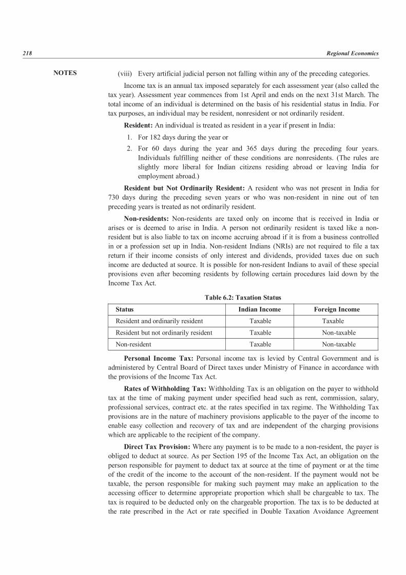
NOTES


(viii) Every artificial judicial person not falling within any of the preceding categories.

Income tax is an annual tax imposed separately for each assessment year (also called thetax year). Assessment year commences from 1st April and ends on the next 31st March. Thetotal income of an individual is determined on the basis of his residential status in India. Fortax purposes, an individual may be resident, nonresident or not ordinarily resident.

Resident: An individual is treated as resident in a year if present in India:

1. For 182 days during the year or2. For 60 days during the year and 365 days during the preceding four years.Individuals fulfilling neither of these conditions are nonresidents. (The rules areslightly more liberal for Indian citizens residing abroad or leaving India foremployment abroad.)

Resident but Not Ordinarily Resident: A resident who was not present in India for730 days during the preceding seven years or who was non-resident in nine out of tenpreceding years is treated as not ordinarily resident.

Non-residents: Non-residents are taxed only on income that is received in India orarises or is deemed to arise in India. A person not ordinarily resident is taxed like a non-resident but is also liable to tax on income accruing abroad if it is from a business controlledin or a profession set up in India. Non-resident Indians (NRIs) are not required to file a taxreturn if their income consists of only interest and dividends, provided taxes due on suchincome are deducted at source. It is possible for non-resident Indians to avail of these specialprovisions even after becoming residents by following certain procedures laid down by theIncome Tax Act.

Table 6.2: Taxation Status

Status Indian Income Foreign Income

Resident and ordinarily resident Taxable Taxable

Resident but not ordinarily resident Taxable Non-taxable

Non-resident Taxable Non-taxable

Personal Income Tax: Personal income tax is levied by Central Government and isadministered by Central Board of Direct taxes under Ministry of Finance in accordance withthe provisions of the Income Tax Act.

Rates of Withholding Tax:Withholding Tax is an obligation on the payer to withholdtax at the time of making payment under specified head such as rent, commission, salary,professional services, contract etc. at the rates specified in tax regime. The Withholding Taxprovisions are in the nature of machinery provisions applicable to the payer of the income toenable easy collection and recovery of tax and are independent of the charging provisionswhich are applicable to the recipient of the company.

Direct Tax Provision:Where any payment is to be made to a non-resident, the payer isobliged to deduct at source. As per Section 195 of the Income Tax Act, an obligation on theperson responsible for payment to deduct tax at source at the time of payment or at the timeof the credit of the income to the account of the non-resident. If the payment would not betaxable, the person responsible for making such payment may make an application to theaccessing officer to determine appropriate proportion which shall be chargeable to tax. Thetax is required to be deducted only on the chargeable proportion. The tax is to be deducted atthe rate prescribed in the Act or rate specified in Double Taxation Avoidance Agreement

NOTES


whichever is beneficial to the assessee. Any person making a payment to any non-residentshall be liable to deduct tax at the rates specified.

Rates of Withholding Tax: Current rates for withholding tax for payment to non-residents are:

1. Interest: 20 percent2. Dividends paid by domestic companies: Nill3. Royalties: 10 percent4. Technical Services: 10 percent5. Any other services:

• Individuals: 30 percent of the income• Companies: 40 percent of the net income.

The above rates are general and are applicable in respect of countries with which Indiadoes not have a Double Taxation Avoidance Agreement (DTAA).

Tax upon Capital GainsCorporate Tax

Definition of a Company: A company has been defined as a juristic person having anindependent and separate legal entity from its shareholders. Income of the company iscomputed and assessed separately in the hands of the company. However, the income of thecompany, which is distributed to its shareholders as dividend, is assessed in their individualhands. Such distribution of income is not treated as expenditure in the hands of company; theincome so distributed is an appropriation of the profits of the company.

Residence of a Company

A company is said to be a resident in India during the relevant previous year if:

1. It is an Indian company.2. If it is not an Indian company but, the control and the management of its affairs is

situated wholly in India.3. A company is said to be non-resident in India if it is not an Indian company and

some part of the control and management of its affairs is situated outside India.

Corporate Sector Tax: The taxability of a company’s income depends on its domicile.Indian companies are taxable in India on their worldwide income. Foreign companies aretaxable on income that arises out of their Indian operations or in certain cases, income that isdeemed to arise in India. Royalty, interest, gains from sale of capital assets located in India(including gains from sale of shares in an Indian company), dividends from Indian companiesand fees for technical services are all treated as income arising in India.

Different Kinds of Taxes Relating to a CompanyMinimum Alternative Tax (MAT): Normally, a company is liable to pay tax on the

income computed in accordance with the provisions of the Income Tax Act, but the Profit andLoss Account of the company is prepared as per provisions of the Companies Act. Therewere large number of companies who had book profits as per their Profit and Loss Accountbut were not paying any tax because income computed as per provisions of the Income TaxAct was either nil or negative or insignificant. In such case, although the companies wereshowing book profits and declaring dividends to the shareholders, they were not paying any

NOTES


income tax. These companies are popularly known as Zero Tax companies. In order to bringsuch companies under the Income Tax Act net, Section 115JA was introduced w.e.f.assessment year 1997-98.

A new tax credit scheme is introduced by which MAT paid can be carried forward forset-off against regular tax payable during the subsequent five year period subject to certainconditions, as under:

1. When a company pays tax under MAT, the tax credit earned by it shall be anamount, which is the difference between the amount payable under MAT and theregular tax. Regular tax, in this case, means the tax payable on the basis of normalcomputation of total income of the company.

2. MAT credit will be allowed carry forward facility for a period of five assessmentyears immediately succeeding the assessment year in which MAT is paid.Unabsorbed MAT credit will be allowed to be accumulated subject to the five-yearcarry forward limit.

3. In the assessment year when regular tax becomes payable, the difference betweenthe regular tax and the tax computed under MAT for that year will be set-offagainst the MAT credit available.

4. The credit allowed will not bear any interest.

Fringe Benefit Tax (FBT): The Finance Act, 2005 introduced a new levy, namelyFringe Benefit Tax (FBT) contained in Chapter XIIH (Sections 115W to 115WL) of theIncome Tax Act, 1961.

Fringe Benefit Tax (FBT) is an additional income tax payable by the employers onvalue of fringe benefits provided or deemed to have been provided to the employees. TheFBT is payable by an employer who is a company; a firm; an association of personsexcluding trusts or a body of individuals; a local authority; a sole trader, or an artificialjuridical person. This tax is payable even where employer does not otherwise have taxableincome. Fringe Benefits are defined as any privilege, service, facility or amenity directly orindirectly provided by an employer to his employees (including former employees) by reasonof their employment and includes expenses or payments on certain specified heads.

The benefit does not have to be provided directly in order to attract FBT. It may still beapplied if the benefit is provided by a third party or an associate of employer or by under anagreement with the employer.

The value of fringe benefits is computed as per provisions under Section 115WC. FBTis payable at prescribed percentage on the taxable value of fringe benefits. Besides, surchargein case of both domestic and foreign companies shall be leviable on the amount of FBT. Onthese amounts, education cess shall also be payable.

Every company shall file return of fringe benefits to the Assessing Officer in theprescribed form by 31st October of the assessment year as per provisions of Section 115WD.If the employer fails to file return within specified time limit specified under the said section,he will have to bear penalty as per Section 271FB.

The scope of Fringe Benefit Tax is being widened by including the employees stockoption as fringe benefit liable for tax. The fair market value of the share on the date of thevesting of the option by the employee as reduced by the amount actually paid by him orrecovered from him shall be considered to be the fringe benefit. The fair market value shallbe determined in accordance with the method to be prescribed by the CBDT.

NOTES


Dividend Distribution Tax (DDT): Under Section 115-O of the Income Tax Act, anyamount declared, distributed or paid by a domestic company by way of dividend shall bechargeable to dividend tax. Only a domestic company (not a foreign company) is liable forthe tax. Tax on distributed profit is in addition to income tax chargeable in respect of totalincome. It is applicable whether the dividend is interim or otherwise. Also, it is applicablewhether such dividend is paid out of current profits or accumulated profits.

The tax shall be deposited within 14 days from the date of declaration, distribution orpayment of dividend, whichever is earliest. Failing to this deposition will require payment ofstipulated interest for every month of delay under Section 115-P of the Act.

Rate of dividend distribution tax to be raised from 12.5 percent to 15 percent ondividends distributed by companies; and to 25 percent on dividends paid by money marketmutual funds and liquid mutual funds to all investors.

Banking Cash Transaction Tax (BCTT): The Finance Act 2005 introduced theBanking Cash Transaction Tax (BCTT) w.e.f. June 1, 2005 and applies to the whole of Indiaexcept in the state of Jammu and Kashmir. BCTT continues to be an extremely useful tool totrack unaccounted monies and trace their source and destination. It has led the Income TaxDepartment to many money laundering and hawala transactions.

BCTT is levied at the rate of 0.1 percent of the value of following ‘taxable bankingtransactions’ entered with any scheduled bank on any single day:

1. Withdrawal of cash from any bank account other than a saving bank account; and2. Receipt of cash on encashment of term deposit(s).

However, Banking Cash Transaction Tax (BCTT) has been withdrawn with effect fromApril 1, 2009.

Securities Transaction Tax (STT): Securities Transaction Tax or turnover tax, as isgenerally known, is a tax that is leviable on taxable securities transaction. STT is leviable onthe taxable securities transactions with effect from 1st October, 2004 as per the notificationissued by the Central Government. The surcharge is not leviable on the STT.

Wealth Tax: Wealth tax, in India, is levied under Wealth Tax Act, 1957. Wealth tax isa tax on the benefits derived from property ownership. The tax is to be paid year after year onthe same property on its market value, whether or not such property yields any income. Underthe Act, the tax is charged in respect of the wealth held during the assessment year by thefollowing persons:

1. Individual2. Hindu Undivided Family (HUF)3. Company

Chargeability to tax also depends upon the residential status of the assessee same as theresidential status for the purpose of the Income Tax Act.

Wealth tax is not levied on productive assets; hence, investments in shares, debentures,UTI, mutual funds, etc. are exempt from it. The assets chargeable to wealth tax are guesthouse, residential house, commercial building, motor car, jewellery, bullion, utensils of gold,silver, yachts, boats and aircrafts, urban land and cash in hand (in excess of ` 50,000 forIndividual and HUF only). However, following will not be included in assets:

1. Assets held as stock in trade.2. A house held for business or profession.

NOTES


3. Any property in nature of commercial complex.4. A house let out for more than 300 days in a year.5. Gold deposit bond.6. A residential house allotted by a company to an Employee, or an Officer, or a

Whole-time Director (gross salary, i.e., excluding perquisites and before StandardDeduction of such Employee, Officer or Director should be less than ` 5,00,000).

The assets exempt from Wealth Tax are ‘Property held under a trust’, Interest of theassessee in the coparcenary property of a HUF of which he is a member, ‘Residentialbuilding of a former ruler’, ‘Assets belonging to Indian repatriates’, one house or a part ofhouse or a plot of land not exceeding 500 sq. mts. (for individual and HUF assessee)

Wealth tax is chargeable in respect of Net wealth corresponding to valuation date whereNet wealth is all assets less loans taken to acquire those assets and valuation date is31st March of immediately preceding the assessment year. In other words, the value of thetaxable assets on the valuation date is clubbed together and is reduced by the amount of debtowed by the assessee. The net wealth so arrived at is charged to tax at the specified rates.Wealth tax is charged @ 1 percent of the amount by which the net wealth exceeds ` 15 lakhs.

Tax Rebates for Corporate Tax: The classical system of corporate taxation isfollowed in India. Domestic companies are permitted to deduct dividends received from otherdomestic companies in certain cases. Inter-company transactions are honoured if negotiatedat arm’s length. Special provisions apply to venture funds and venture capital companies.Long-term capital gains have lower tax incidence. There is no concept of thin capitalization.Liberal deductions are allowed for exports and the setting up on new industrial undertakingsunder certain circumstances. There are liberal deductions for setting up enterprises engaged indeveloping, maintaining and operating new infrastructure facilities and power-generatingunits. Business losses can be carried forward for eight years, and unabsorbed depreciation canbe carried indefinitely. No carry back is allowed. Dividends, interest and long-term capitalgain income earned by an infrastructure fund or company from investments in shares or long-term finance in enterprises carrying on the business of developing, monitoring and operatingspecified infrastructure facilities or in units of mutual funds involved with the infrastructureof power sector is proposed to be tax exempt.

Capital Gains Tax: A capital gain is income derived from the sale of an investment. Acapital investment can be a home, a farm, a ranch, a family business, work of art etc. In mostyears, slightly less than half of taxable capital gains are realized on the sale of corporate stock.The capital gain is the difference between the money received from selling the asset and theprice paid for it. Capital gain also includes gain that arises on ‘transfer’ (includes sale,exchange) of a capital asset and is categorized into short-term gains and long-term gains. Thecapital gains tax is different from almost all other forms of taxation in that it is a voluntarytax. Since the tax is paid only when an asset is sold, taxpayers can legally avoid payment byholding on to their assets—a phenomenon known as the lock-in effect. The scope of capitalasset is being widened by including certain items held as personal effects such asarchaeological collections, drawings, paintings, sculptures or any work of art. Presently, nocapital gain tax is payable in respect of transfer of personal effects as it does not fall in thedefinition of the capital asset. To restrict the misuse of this provision, the definition of capitalasset is being widened to include those personal effects such as archaeological collections,drawings, paintings, sculptures or any work of art. Transfer of above items shall now attractcapital gain tax the way jewellery attracts despite being personal effect as on date.

NOTES


Short-term and Long-term Capital Gains: Gains arising on transfer of a capital assetheld for not more than 36 months (12 months in the case of a share held in a company orother security listed on recognized stock exchange in India or a unit of a mutual fund) prior toits transfer are “short term”. Capital gains arising on transfer of capital asset held for a periodexceeding the aforesaid period are “long term”. Section 112 of the Income Tax Act providesfor the tax on long-term capital gains, at 20 percent of the gain computed with the benefit ofindexation and 10 percent of the gain computed (in case of listed securities or units) withoutthe benefit of indexation.

Double Taxation Relief: Double Taxation means taxation of the same income of aperson in more than one country. This results due to countries following different rules forincome taxation. There are two main rules of income taxation, i.e., (a) Source of income ruleand (b) Residence rule.

As per source of income rule, the income may be subject to tax in the country where thesource of such income exists (i.e., where the business establishment is situated or where theasset/property is located) whether the income earner is a resident in that country or not. Onthe other hand, the income earner may be taxed on the basis of the residential status in thatcountry. For instance, if a person is resident of a country, he may have to pay tax on anyincome earned outside that country as well. Further, some countries may follow a mixture ofthe above two rules. Therefore, problem of double taxation arises if a person is taxed inrespect of any income on the basis of source of income rule in one country and on the basis ofresidence in another country or on the basis of mixture of above two rules.

In India, the liability under the Income Tax Act arises on the basis of the residentialstatus of the assessee during the previous year. In case the assessee is resident in India, healso has to pay tax on the income, which accrues or arises outside India, and also receivedoutside India. The position in many other countries being also broadly similar. It frequentlyhappens that a person may be found to be a resident in more than one country or that the sameitem of his income may be treated as accruing, arising or received in more than one countrywith the result that the same item becomes liable to tax in more than one country. Reliefagainst such hardship can be provided mainly in two ways: (a) Bilateral relief, and(b) Unilateral relief.

(a) Bilateral Relief: The Governments of two countries can enter into DoubleTaxation Avoidance Agreement (DTAA) to provide relief against such DoubleTaxation, worked out on the basis of mutual agreement between the two concernedsovereign states. This may be called a scheme of ‘bilateral relief’ as bothconcerned powers agree as to the basis of the relief to be granted by either of them.

(b) Unilateral Relief: The above procedure for granting relief will not be sufficient tomeet all cases. No country will be in a position to arrive at such agreement with allthe countries of the world for all time. The hardship of the taxpayer, however, is acrippling one in all such cases. Some relief can be provided even in such cases byhome country irrespective of whether the other country concerned has anyagreement with India or has otherwise provided for any relief at all in respect ofsuch double taxation. This relief is known as unilateral relief.

Double Taxation Avoidance Agreement (DTAA)Following are the list of grounds with which India has signed Double Taxation

Avoidance Agreement:

(i) DTAA Comprehensive Agreements with respect to taxes on income.

NOTES


(ii) DTAA Limited Agreement with respect to income of airlines or merchant shipping.(iii) Limited Multilateral Agreement(iv) DTAA Other Agreements or Double Taxation Relief Rules.(v) Specified Associations Agreement

(vi) Tax Information Exchange Agreement (TIEA)

Indirect TaxationSales Tax

Central Sales Tax (CST): Central Sales tax is generally payable on the sale of allgoods by a dealer in the course of inter-state trade or commerce or, outside a state or, in thecourse of import into or, export from India. The ceiling rate on central sales tax (CST), a taxon inter-state sale of goods, has been reduced from 4 percent to 3 percent in the current year.

Value Added Tax (VAT): VAT is a multi-stage tax on goods that is levied acrossvarious stages of production and supply with credit given for tax paid at each stage of valueaddition. Introduction of state level VAT is the most significant tax reform measure at statelevel. The state level VAT has replaced the existing State Sales Tax. The decision toimplement state level VAT was taken in the meeting of the Empowered Committee (EC) ofState Finance Ministers held on June 18, 2004, where a broad consensus was arrived at tointroduce VAT from April 1, 2005. Accordingly, all states/UTs have implemented VAT.

The Empowered Committee, through its deliberations over the years, finalized a designof VAT to be adopted by the States, which seeks to retain the essential features of VAT,while at the same time, providing a measure of flexibility to the States, to enable them tomeet their local requirements. Some salient features of the VAT design finalized by theEmpowered Committee are as follows:

The rates of VAT on various commodities shall be uniform for all the States/UTs. Thereare 2 basic rates of 4 percent and 12.5 percent, besides an exempt category and a special rateof 1 percent for a few selected items. The items of basic necessities have been put in the zerorate bracket or the exempted schedule. Gold, silver and precious stones have been put in the1 percent schedule. There is also a category with 20 percent floor rate of tax, but thecommodities listed in this schedule are not eligible for input tax rebate/set-off. This categorycovers items like motor spirit (petrol), diesel, aviation turbine fuel, and liquor.

There is provision for eliminating the multiplicity of taxes. In fact, all the State taxes onpurchase or sale of goods (excluding Entry Tax in lieu of Octroi) are required to be subsumedin VAT or made VATable.

Provision has been made for allowing ‘Input Tax Credit (ITC)’, which is the basicfeature of VAT. However, since the VAT being implemented is intra-state VAT only anddoes not cover inter-state sale transactions, ITC will not be available on inter-state purchases.Exports will be zero-rated, with credit given for all taxes on inputs/purchases related to suchexports. There are provisions to make the system more business-friendly. For instance, thereis provision for self-assessment by the dealers. Likewise, there is provision of a thresholdlimit for registration of dealers in terms of annual turnover of ` 5 lakh. Dealers with turnoverlower than this threshold limit are not required to obtain registration under VAT and areexempt from payment of VAT. There is also provision for composition of tax liability up toannual turnover limit of ` 50 lakh. Regarding the industrial incentives, the States have been

NOTES


allowed to continue with the existing incentives, without breaking the VAT chain. However,no fresh sales tax/VAT based incentives are permitted.

Roadmap towards GST: The Empowered Committee of State Finance Ministers hasbeen entrusted with the task of preparing a roadmap for the introduction of national levelgoods and services tax with effect from 01 April 2007. The move is towards the reduction ofCST to 2 percent in 2008, 1 percent in 2009 and 0 percent in 2010 to pave way for theintroduction of GST (Goods and Services Tax).

Excise Duty: Central Excise duty is an indirect tax levied on goods manufactured inIndia. Excisable goods have been defined as those, which have been specified in the CentralExcise Tariff Act as being subjected to the duty of excise.

There are three types of Central Excise duties collected in India, viz.,

1. Basic Excise Duty: This is the duty charged under Section 3 of the Central Excisesand Salt Act,1944 on all excisable goods other than salt which are produced ormanufactured in India at the rates set forth in the schedule to the Central ExciseTariff Act,1985.

2. Additional Duty of Excise: Section 3 of the Additional duties of Excise (Goods ofSpecial Importance) Act, 1957 authorizes the levy and collection in respect of thegoods described in the Schedule to this Act. This is levied in lieu of Sales Tax andshared between Central and State Governments. These are levied under differentenactments like medicinal and toilet preparations, sugar etc. and other industriesdevelopment etc.

3. Special Excise Duty: As per the Section 37 of the Finance Act, 1978, SpecialExcise Duty was attracted on all excisable goods on which there is a levy of BasicExcise Duty under the Central Excises and Salt Act,1944. Since then, each year,the relevant provisions of the Finance Act specifies that the Special Excise Dutyshall be or shall not be levied and collected during the relevant financial year.

Customs Duty: Custom or import duties are levied by the Central Government of Indiaon the goods imported into India. The rate at which customs duty is leviable on the goodsdepends on the classification of the goods determined under the Customs Tariff. The CustomsTariff is generally aligned with the Harmonized System of Nomenclature (HSL). In line withaligning the customs duty and bringing it at par with the ASEAN level, government hasreduced the peak customs duty from 12.5 percent to 10 percent for all goods other thanagriculture products. However, the Central Government has the power to generally exemptgoods of any specified description from the whole or any part of duties of customs leviablethereon. In addition, preferential/concessional rates of duty are also available under thevarious Trade Agreements.

Service Tax: Service tax was introduced in India way back in 1994 and started withmere three basic services, viz., general insurance, stock broking and telephone. Today, thecounter services subject to tax have reached over 100. There has been a steady increase in therate of service tax. From a mere 5 percent, service tax is now levied on specified taxableservices at the rate of 12 percent of the gross value of taxable services. However, on accountof the imposition of education cess of 3 percent, the effective rate of service tax is at12.36 percent.

Union Budget 2013-14: Latest Union Budget for the year 2013-14 has been announcedby the Financed Minister on 28th of February 2013. Here are the highlights of the keyfeatures of Direct and Indirect Tax Proposals:

NOTES


Tax ProposalsDirect Taxes: According to the Finance Minister, there is a little room to give away tax

revenues or raise tax rates in a constrained economy. Even a moderate increase in thethreshold exemption will put hundreds of thousands of taxpayers outside Tax Net. However,relief for taxpayers in the first bracket of USD 0.004 million to USD 0.009 million. A taxcredit of USD 36.78 to every person with total income upto USD 0.009 million. Surcharge of10 percent on persons (other than companies) whose taxable income exceed USD 0.18million to augment revenues. Increase surcharge from 5 percent to 10 percent on domesticcompanies whose taxable income exceed USD 1.84 million. In case of foreign companieswho pay a higher rate of corporate tax, surcharge to increase from 2 to 5 percent, if thetaxable income exceeds USD 1.84 million. In all other cases such as dividend distribution taxor tax on distributed income, current surcharge increased from 5 to 10 percent. Additionalsurcharges to be in force for only one year. Education cess to continue at 3 percent.Permissible premium rate increased from 10 percent to 15 percent of the sum assured byrelaxing eligibility conditions of life insurance policies for persons suffering from disabilityand certain ailments. Contributions made to schemes of Central and State Governmentssimilar to Central Government Health Scheme, eligible for Section 80D of the Income TaxAct. Donations made to National Children Fund eligible for 100 percent deduction.Investment allowance at the rate of 15 percent to manufacturing companies that invest morethan USD 1.84 million in plant and machinery during the period 1st April 2013 to 31st March2015. Eligible date for projects in the power sector to avail benefit under Section 80-IAextended from 31st March, 2013 to 31st March, 2014. Concessional rate of tax of 15 percenton dividend received by an Indian company from its foreign subsidiary proposed to continuefor one more year. Securitization Trust to be exempted from Income Tax. Tax to be levied atspecified rates only at the time of distribution of income for companies, individual, HUF etc.No further tax on income received by investors from the Trust. Investor Protection Fund ofdepositories exempt from income tax in some cases. Parity in taxation between IDF-MutualFund and IDF-NBFC. A Category IAIF set up as Venture capital fund allowed pass throughstatus under Income Tax Act. TDS at the rate of 1 percent on the value of the transfer ofimmovable properties where consideration exceeds USD 0.092 million. Agricultural land tobe exempted. A final withholding tax at the rate of 20 percent on profits distributed byunlisted companies to shareholders through buyback of shares. Proposal to increase the rateof tax on payments by way of royalty and fees for technical services to non-residents from 10percent to 25 percent. Reductions made in rates of Securities Transaction Tax in respect ofcertain transaction. Proposal to introduce Commodity Transaction Tax (CTT) in a limitedway. Agricultural commodities will be exempted. Modified provisions of GAAR will comeinto effect from 1st April, 2016. Rules on Safe Harbour will be issued after examining thereports of the Rangachary Committee appointed to look into tax matters relating toDevelopment Centres and IT sector and Safe Harbour rules for a number of sectors. Fifthlarge taxpayer unit to open at Kolkata shortly. A number of administrative measures such asextension of refund banker system to refund more than USD 918.86, technology basedprocessing, extension of e-payment through more banks and expansion in the scope ofannual information returns by Income Tax Department.

Indirect Taxes1. No change in the normal rates of 12 percent for excise duty and service tax.2. No change in the peak rate of basic customs duty of 10 percent for non-agricultural

products.

NOTES


Customs: Period of concession available for specified part of electric and hybridvehicles extended upto 31st March, 2015. Duty on specified machinery for manufacture ofleather and leather goods including footwear reduced from 7.5 to 5 percent. Duty onpre-forms precious and semi-precious stones reduced from 10 to 2 percent. Export duty onde-oiled rice bran oil cake withdrawn. Duty of 10 percent on export of unprocessed ilmeniteand 5 percent on export on ungraded ilmenite. Concessions to aircraft maintenance, repairand overhaul (MRO) industry. Duty on Set Top Boxes increased from 5 to 10 percent. Dutyon raw silk increased from 5 to 15 percent. Duties on Steam Coal and Bituminous Coalequalized and 2 percent custom duty and 2 percent CVD levied on both kinds coal. Duty onimported luxury goods such as high-end motor vehicles, motor cycles, yachts and similarvessels increased. Duty free gold limit increased to USD 918.86 in case of male passengerand USD 1,837.47 in case of a female passenger subject to conditions.

Excise Duty: Central Excise duty is an indirect tax levied on those goods which aremanufactured in India and are meant for home consumption. The taxable event is‘manufacture’ and the liability of central excise duty arises as soon as the goods aremanufactured. It is a tax on manufacturing, which is paid by a manufacturer, who passes itsincidence on to the customers.

The term “excisable goods” means the goods which are specified in the First Scheduleand the Second Schedule to the Central Excise Tariff Act,1985 , as being subject to a duty ofexcise and includes salt.

The term “manufacture” includes any process, incidental or ancillary to the completionof a manufactured product and which is specified in relation to any goods in the section orchapter notes of the First Schedule to the Central Excise Tariff Act,1985 as amounting tomanufacture or which, in relation to the goods specified in the Third Schedule, involvespacking or repacking of such goods in a unit container or labelling or re-labelling ofcontainers including the declaration or alteration of retail sale price on it or adoption of anyother treatment on the goods to render the product marketable to the consumer.

As incidence of excise duty arises on production or manufacture of goods, the law doesnot require the sale of goods from place of manufacture, as a mandatory requirement.Normally, duty is payable on ‘removal’ of goods. The Central Excise Rules provide thatevery person who produces or manufactures any ‘excisable goods’, or who stores such goodsin a warehouse, shall pay the duty leviable on such goods in the manner provided in rules orunder any other law. No excisable goods, on which any duty is payable, shall be ‘removed’without payment of duty from any place, where they are produced or manufactured, or from awarehouse, unless otherwise provided. The word ‘removal’ cannot be necessarily equatedwith sale. Here, the removal may be for Sale, Transfer to depot etc., Captive consumption,Transfer to another unit, Free distribution. Thus, it can be seen that duty becomes payableirrespective of whether the removal is for sale or for some other purpose.

Service Tax

1. Maintain stability in tax regime. Vocational courses offered by institutes affiliatedto the State Council of Vocational Training and testing activities in relation toagricultural produce also included in the negative list for service tax. Exemption ofService Tax on copyright on cinematography limited to films exhibited in cinemahalls. Proposals to levy Service Tax on all air conditioned restaurant.

NOTES


2. For homes and flats with a carpet area of 2,000 sq.ft. or more or of a value of USD0.18 million or more, which are high-end constructions, where the component ofservices is greater, rate of abatement reduced from from 75 to 70 percent.

3. Out of nearly 1.7 million registered assesses under Service Tax only 0.7 millionfile returns regularly. Need to motivate them to file returns and pay tax dues. Aone-time scheme called ‘Voluntary Compliance Encouragement Scheme’ proposedto be introduced. Defaulter may avail of the scheme on condition that he filestruthful declaration of Service Tax dues since 1st October, 2007.

4. Tax proposals on Direct Taxes side estimated to yield to USD 2,444.32 million andon the Indirect Tax side USD 863.68 million.

Good and Services Tax: A sum of USD 1,653.78 million towards the first installmentof the balance of CST compensation provided in the budget. Work on draft GSTConstitutional Amendment Bill and GST Law expected to be taken forward.

6.6 TRANSFER PROGRAMMES (INTERNATIONAL TECHNOLOGYTRANSFER PROGRAMME)

Objectives and Nature of ActivitiesThe objective of International Technology Transfer Programme (ITTP) is to promote

international technology transfer and trade with India as focus. Activities under theprogramme are focused in the following three areas.

Documentation of Technology Export Performance and Capabilities: Readilyavailable and updated documentation on technology related export performance andcapabilities of our industrial units, R&D organizations and other export promotion agencieshelps in policy formulation, technology related business promotion, keeping track of pastperformances, course correction and setting targets for the future. Documents andpublications serve as the basic form of visible output of any activity. The programmesupports activities towards preparation of such documentation.

Showcasing and Demonstration of Technology Export Capabilities: It is essential towidely publicize our technological capabilities for promotion of business ventures abroad andformulation of technology transfer projects involving foreign agencies. Sensitization of tradepromotion bodies and industry associations towards enhanced thrust on technology and valueadded technology intensive products is important in view of the rapidly growing globalcompetition. The programme supports organization of technology based trade fairs,participation of technology intensive organizations in such fairs, setting up of TechnologyTrade Facilitation Centres, organization of Training-cum-Awareness Programmes foroverseas participants, etc.

Facilitation of Technology Transfer and Trade at the Firm Level: Besides broad-based support provided under the above two categories, it is essential to provide hand-holdingand support at the firm level in order to facilitate technology transfer negotiations, draft/finalize MOUs/Agreements and materialize business deals and contracts. The programmesupports organization of area-specific buyer-seller meets in India and abroad which provide aplatform for one-to-one interactions between interested business partners.

NOTES


Projects/ActivitiesCompendium on Technology Exports – An Illustrative Compilation of Exported

and Exportable Technologies from India: The publication brought out in collaborationwith Indian Institute of Foreign Trade (IIFT), New Delhi, contains information ontechnologies actually exported as well as technologies having potential for exports. Out of the377 organizations covered in the recent publication, 248 organizations have reportedtechnology intensive exports of ` 156,849 million during 2001-02 and the remainingorganizations have claimed to be in possession of exportable technologies/projects.According to the findings of the publication, growth rate of high technology exports is higher,compared to medium and low technology exports and average exports of high technologyexporting organizations are also higher than medium and low technology exportingorganizations. The organizations engaged in high technology exports also have a high R&Dintensity. Among the 248 exporting organizations covered in the publication,94 organizations entered into foreign collaborations.

Newsletter on Technology Exports: Publication of a quarterly Newsletter onTechnology Exports, initiated by IIFT during the year 1998-99 with the support of DSIR wascontinued during the year. The newsletter is being compiled by Indian Institute of ForeignTrade, New Delhi under the guidance of an Editorial Board, comprising of representativesfrom DSIR, IIFT, Exim Bank, Ministry of External Affairs and ITPO. The contents ofnewsletter include details on technology export related policies, technology developments –globally as well as within the country, joint-ventures abroad, India’s achievements intechnology related exports, technology offers and requests etc. and thereby appreciated byindustry, embassies/missions, export promotion councils and other international bodies.

Technology Trade Pavilion at India International Trade Fair, New Delhi: Theobjective of setting up a Technology Trade Pavilion is to promote display and disseminationof information related to technological capabilities, high value added products andtechnologies of companies and organizations including R&D laboratories, academicinstitutions, product design institutions, consultants etc. The Technology Trade Pavilion wassetup jointly by DSIR and India Trade Promotion Organization (ITPO) for the eighth time insuccession since 1997. Awards for Technology Innovation and Best Display were alsoannounced. In order of merit, technology innovation awards were bagged by CSIR, IIT-Bombay and Dip Craft Industries and best display awards were bagged by Coral Industries,National Productivity Council and National Research Development Corporation. TheTechnology Trade Pavilion helped in promoting one-to-one interactions and businessnegotiations between the participating organizations displaying their technology intensiveproducts, technologies, machinery, services, etc. and potential customers of Indiantechnology and services.

Technology Export Development Organization: The main objective of theTechnology Export Development Organization (TEDO) – a Cell jointly setup by DSIR andCII in April 2000, is to promote and support technology and technology intensive exportsthrough collaborative efforts of government, industry, research and academic institutions,financial institutions and other export promotion agencies. TEDO focuses on four areas,namely Agro/Food Processing, Light Engineering, Indian Systems of Medicine andHomeopathy and Chemicals and Pharmaceuticals. Nature of TEDO activities range fromstudies, training and awareness programmes to missions, fairs, seminars and technologydemonstrations.

NOTES


Strategic Approach to Strengthening the International Competitiveness ofKnowledge-based Industries: Objectives of the research study carried out by Research andInformation Systems for the Non-aligned and Other Developing Countries were to examine:India’s export structure in terms of its knowledge intensity compared to some of the South-East Asian countries; emerging patterns of FDI inflows and the participation of MNCs inknowledge-based industries; outward investments by Indian enterprises in knowledge-basedindustries; and export oriented manufacture by MNCs and draw up strategies forstrengthening the international competitiveness of knowledge-based industries in the country.

Centre for International Trade in Technology (CITT): The main objective of theCentre is to conduct research on the emerging issues relating to technology trade agreementsof WTO and other international arrangements such as, TRIPs, TBT, GATS, etc. and toidentify specific technology related export opportunities for India and to develop trainingexpertise in the area of technology export management. An agreement on the Centre betweenDSIR and IIFT was signed on June 4, 2001.

International Programme on Design as Strategy for Development and Quality ofLiving: The above programme was organized by National Institute of Design (NID),Ahmedabad during January 17-21, 2005 with the support of DSIR. The objective was toproject India as the outsourcing destination for industrial and product design services. Thefaculty for the programme was drawn from National Institute of Design (NID) and practicingdesign entrepreneurs, experts and consultants. The programme was attended by around25 participants, who were drawn from South Africa, Iran, Tanzania, Sri Lanka etc. Theparticipants were given a glimpse of industrial design capabilities and achievements of ourdesign institutions, which unfolded opportunities for design collaborations between Indianagencies and foreign participants.

National Awareness-cum-Training Programme on Competitive Advantagethrough Design: The above programme was organized by National Institute of Design (NID),Ahmedabad with the support of DSIR. The objective was to demonstrate the potential ofindustrial design in achieving competitive advantage. The programme included lecturesessions by expert faculty drawn from NID and professional design organizations and fieldvisits to industrial units which have successfully demonstrated the potential of industrial andproduct design in fetching rich dividends.

Technology Trade Facilitation Centre at National Research DevelopmentCorporation (NRDC): A Technology Trade Facilitation Centre was set up at NRDC in July2003 with the support of DSIR. Technology Trade Facilitation Centre is a proactive approachto catalyze technology intensive and high value added exports from Indian industry/R&Destablishments and is expected to provide an exposure to small and medium enterprises(willing to export their hi-tech products and processes) to look at international customers andforeign markets requirements. The following criteria is used for selection of companies inTechnology Trade Facilitation Centre.:

(i) Any company that is manufacturing a hi-tech product/equipment/machinery whichis being exported or has export potential.

(ii) Any company that has commercialized a technology and is willing tolicense/transfer it, within the country or abroad.

(iii) Any organization which can offer a complete technology package or a technologyproject on a turnkey basis.

NOTES


During the year, 10 new companies were selected for participation in the TechnologyTrade Facilitation Centre. These companies were: Sahajanand Laser Technology, Ahmedabad;International Tractors Ltd., Hoshiarpur; etc.

Profiles of Exportable Technologies from SMEs in the Delhi Region: NationalFoundation of Indian Engineers (NAFEN), New Delhi carried out a project on Compilationof Profiles of Exportable Technologies from SMEs in and around Delhi including Faridabad,Gurgaon, Noida and Ghaziabad with the support of DSIR. A report containing 22 profiles ofexportable technologies/projects from SMEs in the targeted region was brought out. TheProfiles contain information such as brief technology description, profile of the companyincluding details such as installed capacity, production, turnover, exports, manpower, usage ofraw material, etc. and a profile of project based on exportable technology, including detailssuch as estimated project cost, land, machinery, manpower and raw material requirements, etc.

Study on Exploring Commercialization of Patents Taken Abroad by Indians –WITT: The study was conducted by Waterfalls Institute of Technology Transfer (WITT),New Delhi with the support of DSIR. It aimed at collecting and analyzing data relating topatents filed abroad by Indians, with a view to study their potential for earlycommercialization and suggest measures for more effective patent commercialization. Thetarget population for the study was around 200 R&D organizations, institutions, in-houseR&D units of export oriented industries and individuals.

6.7 FISCAL RESPONSES OF POWER LEVEL GOVERNMENTS

Contagion from the global crisis necessitated use of fiscal stimulus measures in Indiaduring 2008-10 in order to contain a major slowdown in economic growth. Given the usualdownward inflexibility of fiscal deficit once it reaches a high level, as has been experiencedby India in the past, there could be medium-term implications for the future Inflation path,which must be recognized while designing the timing and speed of fiscal exit. Inflation, attimes, may become effectively a fiscal phenomenon, since the fiscal stance could influencesignificantly the overall monetary conditions. Fiscal deficit could be seen to influence theInflation process either through growth of base money created by the RBI (i.e., net RBI creditto the Government) or through higher aggregate demand associated with an expansionaryfiscal stance (which could increase growth in broad money). The potential Inflation riskshould work as an important motivating factor to ensure a faster return to the fiscalconsolidation path in India, driven by quality of adjustment with appropriate rationalizationof expenditure, rather than waiting for revenue buoyancy associated with sustained robustgrowth to do the job automatically. The importance of fiscal space in the India specificcontext needs to be seen in terms of not only the usual output stabilization role of fiscalpolicy but also the occasional need for use of fiscal measures to contain such Inflationarypressures that may arise from temporary but large supply shocks.

Fiscal stimulus emerged as the key universal instrument of hope in almost every countryaround the world, when the financial crisis in the advanced economies snowballed into asynchronized global recession.

In India, the fiscal response to the global crisis was swift and significant, even thoughIndia clearly avoided a financial crisis at home and also continued to be one of the fastestgrowing economies in the world in a phase of deep global recession. Despite the absence ofany need to bailout the financial system, it is the necessity to partly offset the impact ofdeceleration in private consumption and investment demand on economic growth, which

NOTES


warranted adoption of an expansionary fiscal stance. One important consequence of this,though, was the significant deviation from the fiscal consolidation path and the resultantincrease in the fiscal deficit levels over two consecutive years (2008-10).

The immediate impact of the higher levels of fiscal deficit on Inflation in India could beseen as almost negligible, since: (a) the expansionary fiscal stance was only a partial offsetfor the deceleration in private consumption and investment demand, as the output gap largelyremained negative, indicating no risk to Inflation in the near term; and (b) despite largeincrease in the borrowing programme of the Government to finance the deficit, there was nocorresponding large expansion in money growth, since demand for credit from the privatesector remained depressed. Thus, neither aggregate demand nor monetary expansionassociated with larger fiscal deficits posed any immediate concern on the Inflation front.

The future risks to Inflation in India from fiscal stimulus, thus, could arise from thedownward inflexibility of the deficit levels and with revival in demand for credit from theprivate sector and consolidation of growth around the potential, the fiscal constraint could bemanifested in the form of pressures on both aggregate demand and money supply. Surges incapital flows could complicate the situation further. Macroeconomic variables are generallyinterrelated in a complex manner. Therefore, a deeper understanding of Inflation dynamicswould involve analyzing its relationship with macroeconomic variables such as deficit,money supply, public debt, external balance, exchange rate, output gap, global inflation andcommodity prices, and interest rates. In the literature, particularly in the developing countrycontext, simple models are, however, often used to analyze the Inflationary impact of fiscaldeficit. This largely reflects the role of fiscal dominance, which has often been a phenomenonin many developing countries. Thus, fiscal-based theories of Inflation are more common inthe literature of developing countries. On the other hand, for developed countries, fiscalpolicy is often considered to be unimportant for inflation determination, at least on theoreticalgrounds, as the desire to obtain seigniorage revenue plays no obvious role in the choice ofmonetary policy.

In the Indian context also, there are several studies analyzing the nexus betweengovernment deficits, money supply and Inflation. The findings of these studies generallypoint to a self-perpetuating process of deficit-induced inflation and inflation-induced deficit,besides the overall indication that government deficits represent an important determinant ofInflation However, extending the period of analysis further beyond the automaticmonetization phase, Ashra et al. found no-long relationship between fiscal deficit and netRBI credit to the Government and the latter with broad money supply. Thus, they concludedthat there is no more any rationale for targeting fiscal deficit as a tool for stabilization. On theother hand, according to Khundrakpam and Goyal, recent data and ARDL approach inanalysis, it is found that government deficit continues to be a key factor causing incrementalreserve money creation and overall expansion in money supply, which lead to Inflation.

The Challenge of Fiscal Exit – What is Important for India?

The unprecedented stimulus that was used across countries to avert another GreatDepression is widely believed to have shown the seeds of the next crisis. Public debt levels inthe advanced economies are projected to explode to levels never seen during peacetime,leaving almost no fiscal space for managing other shocks to the economies in future, besidessignificantly constraining normalization of overall macroeconomic conditions. Some of theprojected debt figures look uncomfortably high – revealing in true sense the trade-offsinvolved in policy options. A better today ensured through policy interventions could enhancerisks for the future. In the case of sub-prime crisis, the impact on the world economy will be

NOTES


permanent and is expected to persist over several decades through the channel of high publicdebt.

What then is the dimension of the challenge we are facing today? IMF projectionsindicate that in the G-20 advanced economies, Government debt would reach 118 percent ofGDP in 2014, which will be 40 percent higher than the pre-crisis levels. Consolidating thelevel to about 60 percent of GDP by 2030 would require raising the average structuralprimary balance by 8 percent of GDP, which is not easy, though not impossible. But thisorder of adjustment will involve other costs. One could first see why the adjustment optionsmay not be easy and then what other costs could result from sustained high levels of publicdebt.

The Costs of Sustained High Levels of Public Debt: A critical part of the policychallenge associated with high public debt is to recognize upfront the costs for the economy,without being too alarmist. Some of the costs seem obvious, even though because of the non-linearity in the relationships between key evolving macroeconomic variables, it may not beeasy to quantify them. Some of these obvious costs could be:

(a) Lack of fiscal space to deal with future shocks, including future downturns inbusiness cycles.

(b) Pressure on interest rates and crowding-out of resources from the private sector.This effect is not visible as yet because of weak private demand and expansionarymonetary policies. As private demand recovers and monetary policy cycles turnaround, potential risks will materialize. Three specific channels could exertpressure on the interest rate: (i) larger fiscal imbalances would imply lowerdomestic savings, (ii) increase in risk premia, as market would differentiatebetween debt levels and expect a premium in relation to the perceived risk, whichis already evident after the experience of Dubai World and Greece, and (iii) higherinflation expectations that would invariably result from high levels of debt, whichwill be reflected in the nominal interest rates.

(c) Pressure on central banks to dilute their commitment to and focus on price stability.In this context, one may see the Inflation tolerance levels of central banks rising.The IMF’s argument that raising the Inflation target in advanced economies from2 percent to 4 percent may not add significant distortions to the economies shouldalso be carefully examined by central banks. One must recognize why some feelthat return to pre-crisis levels of central bank independence with focus on pricestability would be critical to improve the future macroeconomic conditions, giventhe large debt overhang. Price stability will be critical to ensure high growth, whichin turn can effectively contribute to debt consolidation without imposing costs ofadjustments through other options. The extent of dilution of central bankindependence may also increase if financial stability is made an explicit mandate ofcentral banks.

Fiscal Exit in India: India was on a sustained path of fiscal consolidation prior to theglobal crisis, conditioned by the discipline embodied in the Fiscal Responsibility and BudgetManagement (FRBM) Act, 2003. The FRBM rules required phased reduction in fiscal deficitto 3 percent of GDP by end-March 2009, with commitment to also eliminate revenue deficitby that time. The progress on fiscal consolidation turned out to be faster than initiallyexpected, as high growth during the five year period 2003-08 ensured better revenuebuoyancy. Fiscal deficit as percentage of GDP fell from 4.5 percent in 2003-04 to 2.6 percentin 2007-08, leading to attainment of the target one year before what was initially set under the

NOTES


FRBM rules in 2004. Revenue deficit also declined from 3.6 percent of GDP to 1.1 percent ofGDP during the corresponding period. The FRBM, thus, had created considerable fiscal space,led by revenue buoyancy, when the impact of the global recession on domestic activitieswarranted introduction of anti-crisis fiscal response. Some have viewed the fiscalconsolidation as a favourable macroeconomic condition that contributed to India’s shift to thehigher growth trajectory, even though it is a fact that fiscal consolidation resulted primarilybecause of high growth.

When the global crisis started to spread, despite perceptions of decoupling and a soundfinancial system at home, there was a clear risk of slowdown in Indian growth, which had tobe arrested through the appropriate policy response. Because of the heightened uncertaintyand the black swan nature of the series of adverse developments that unfolded after thebankruptcy of Lehman Brothers, the Indian policy response had to be swift and significant,with a heavy accent on adequate precaution. Two major fiscal decisions that were takenearlier, i.e., the farm debt waiver scheme and the Sixth Pay Commission award, worked likeexpansionary stimulus, where the decision lag was almost zero, since the decisions had beentaken and partly implemented even before the crisis-led need for fiscal stimulus wasrecognized. The subsequent crisis related fiscal stimulus was delivered in the form of tax cutsas well as higher expenditure, dominated by revenue expenditure, as the deceleration inprivate consumption expenditure turned out to be significant, which needed to be partly offsetby higher government expenditure. Reflecting the expansionary fiscal stance – involving adeliberate deviation from the fiscal consolidation path – the fiscal deficit of the CentralGovernment rose from 2.6 percent of GDP in 2007-08 to 5.9 percent in 2008-09 and furtherto 6.7 percent in 2009-10. Even the State Governments, which were progressing well onfiscal consolidation – driven partly by the incentives from the Twelfth Finance Commission –experienced a setback to the process, resulting primarily from pressures on revenues andcentral transfers associated with the economic slowdown as well as the compelling demand tomatch the pay revision already announced for Central Government employees. Gross fiscaldeficit of the states, which had improved to 1.5 percent of GDP by 2007-08, expanded to3.2 percent of GDP in 2009-10.

The role of the expansionary fiscal stance adopted by both the Central and the StateGovernments has to be seen in the context of the fact that private consumption demand,which accounts for close to 60 percent of aggregate demand, exhibited sharp deceleration ingrowth, from 9.8 percent in 2007-08 to 6.8 percent and 4.1 percent in the subsequent twoyears. Government consumption expenditure, which accounts for just about 10 percent ofaggregate demand, had to be stepped up significantly to partially offset the impact of thesharp deceleration in the growth of private consumption demand. Reflecting the fiscalstimulus, growth in government consumption expenditure was as high as 16.7 percent in2008-09, as a result of which the contribution of government expenditure to the overallgrowth in aggregate demand rose almost threefold – from 10.4 percent in 2007-08 to33.6 percent in 2008-09. The fiscal stance, thus, had a clear role in arresting sharperslowdown in economic growth.

Given the possibility of a weak fiscal position operating as a drag on economic growthin the medium-run – through crowding-out pressures, besides the scope for causing higherInflation – the need for faster return to fiscal consolidation path was recognized quite early inIndia, which was articulated and emphasized by the Reserve Bank in its policy statements, assigns of stronger recovery in growth started to emerge. By the time the Budget for 2010-11was announced in February 2010, better evidence on broad-based momentum in recovery

NOTES


created the space for gradual roll back of some of the fiscal measures that were taken inresponse to the crisis. At the macro level, while gross fiscal deficit has been budgeted lowerat 5.5 percent of GDP, net market borrowing programme has also been scaled down by morethan 10 percent. In terms of specific measures, some of the stimulus-led tax cuts have beenrolled back, greater non-tax revenue from disinvestments and auction of 3-G/BWA spectrumhas been realized and growth in non-plan expenditure has been significantly curtailed to4.1 percent in 2010-11 from 26.0 percent in the previous year, much of which will result fromrationalization of subsidies. More importantly, indicating the resolve to return to the fiscalconsolidation process, a Medium Term Fiscal Policy Statement (MTFPS) has been issuedalong with plans for tax reforms, both direct and indirect. As per the MTFPS, there will beannual rolling targets for revenue deficit and gross fiscal deficit so as to reach 2.7 percent and4.1 percent of GDP, respectively, by 2012-13. Goods and Services Tax (GST) and Direct TaxCode (DTC), to be implemented in 2011-12, will be critical components of the fiscalconsolidation, which could help in improving the tax to GDP ratio from 10.8 percent in2010-11 to 11.8 percent in 2012-13. Reflecting the planned fiscal consolidation, total debtliabilities of the Central Government could also be expected to moderate from 51.5 percent ofGDP in 2009-10 to 48.2 percent of GDP in 2012-13. The Indian approach to fiscal exit – interms of both adoption of specific fiscal consolidation measures in sync with the recovery andannouncement of medium-term targets for phased consolidation – reflects the recognition inthe sphere of policy-making of the importance of a disciplined fiscal environment forsustainable high growth.

The quality of fiscal adjustment, however, must receive greater attention, given themedium-term double digit growth objective. Like the previous phase of fiscal consolidationduring 2004-08, stronger recovery in growth will improve revenue buoyancy. Moreover,given the fact that a large part of the government borrowing (excluding the part invested byFIIs) is financed domestically, the sovereign risk concerns would also remain contained.These favourable aspects, however, should not dilute the focus on consolidation from theexpenditure side. Even if gross fiscal deficit for 2010-11 has been budgeted to decline to5.5 percent of GDP from 6.7 percent in the previous year, that may not signal any majormove in the direction of structural consolidation, if one removes the one-off componentsfrom the revenue and expenditure sides. Adjusted for disinvestment and 3-G/BWA auctionproceeds on the revenue side, and farm debt waiver and Sixth Pay Commission arrears on theexpenditure side, the reduction in gross fiscal deficit as percent of GDP would be much less,i.e., by 0.3 percent as against 1.2 percent envisaged in the Budget. The magnitude and qualityof fiscal adjustment could have a significant conditioning influence on India’s medium-termgrowth prospects.

In the absence of faster and better quality fiscal adjustment, at least four major risks tomacroeconomic conditions could be envisaged: (a) the decline in domestic savings, led by thefall in public sector savings, which will lower the potential output path, (b) higher overallinterest rates, when the revival in demand for credit from the private sector starts competingwith the borrowing programme of the government, (c) limit the capacity to manage theexchange rate and the domestic liquidity impact of possible surges in capital flows, since theuse of sterilization options like the MSS could exert further pressures on the interest rates,and thereby lead to even higher inflows, and (d) may even force reversal of reforms, such asuse of higher SLR requirements for banks or even introduction of SLR for non-bankingentities in the financial system to create a captive market for the government borrowingprogramme. These possible potential implications signify why fiscal discipline is so critical ina market based economy. Often, in the search for easy solutions, direct or indirect

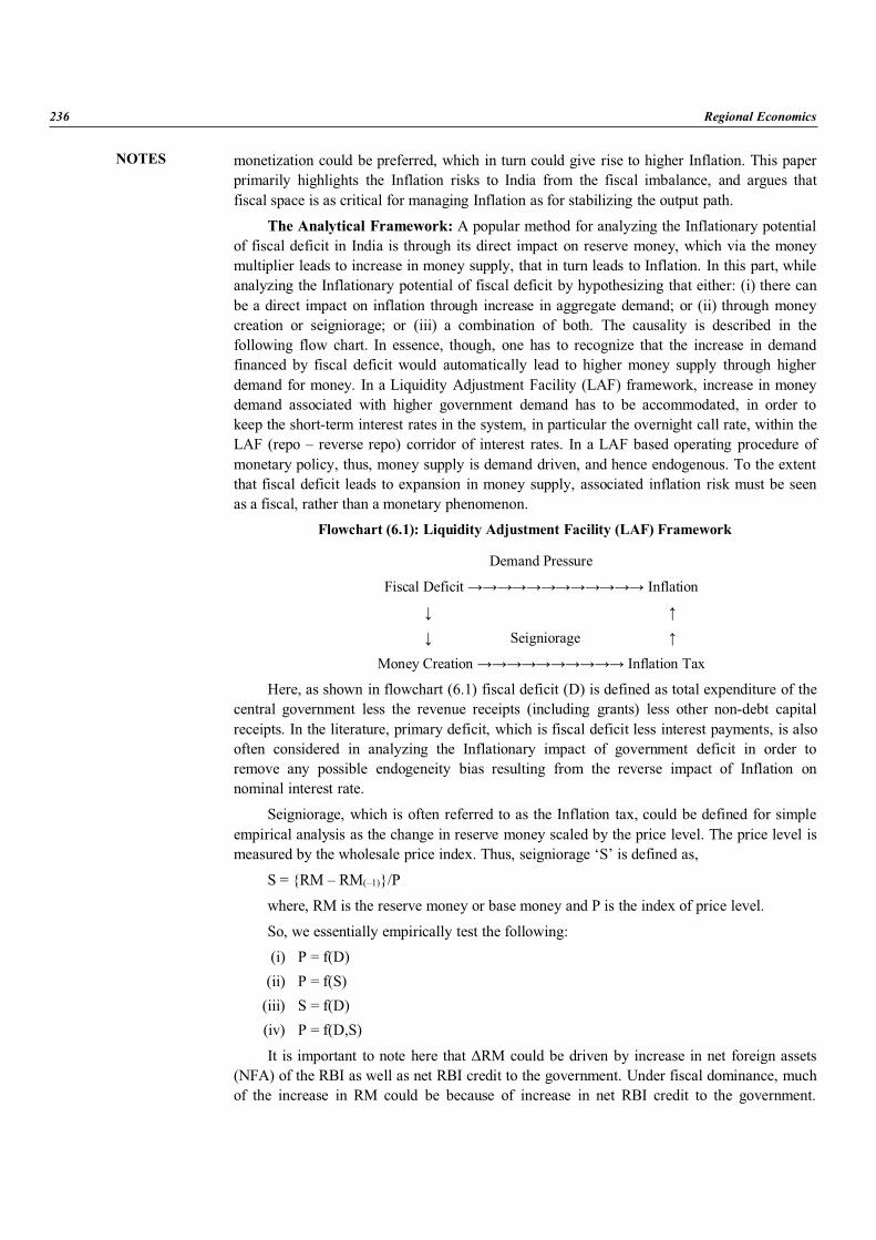
NOTES


monetization could be preferred, which in turn could give rise to higher Inflation. This paperprimarily highlights the Inflation risks to India from the fiscal imbalance, and argues thatfiscal space is as critical for managing Inflation as for stabilizing the output path.

The Analytical Framework: A popular method for analyzing the Inflationary potentialof fiscal deficit in India is through its direct impact on reserve money, which via the moneymultiplier leads to increase in money supply, that in turn leads to Inflation. In this part, whileanalyzing the Inflationary potential of fiscal deficit by hypothesizing that either: (i) there canbe a direct impact on inflation through increase in aggregate demand; or (ii) through moneycreation or seigniorage; or (iii) a combination of both. The causality is described in thefollowing flow chart. In essence, though, one has to recognize that the increase in demandfinanced by fiscal deficit would automatically lead to higher money supply through higherdemand for money. In a Liquidity Adjustment Facility (LAF) framework, increase in moneydemand associated with higher government demand has to be accommodated, in order tokeep the short-term interest rates in the system, in particular the overnight call rate, within theLAF (repo – reverse repo) corridor of interest rates. In a LAF based operating procedure ofmonetary policy, thus, money supply is demand driven, and hence endogenous. To the extentthat fiscal deficit leads to expansion in money supply, associated inflation risk must be seenas a fiscal, rather than a monetary phenomenon.

Flowchart (6.1): Liquidity Adjustment Facility (LAF) Framework

Demand Pressure

Fiscal Deficit Inflation

Seigniorage

Money Creation Inflation Tax

Here, as shown in flowchart (6.1) fiscal deficit (D) is defined as total expenditure of thecentral government less the revenue receipts (including grants) less other non-debt capitalreceipts. In the literature, primary deficit, which is fiscal deficit less interest payments, is alsooften considered in analyzing the Inflationary impact of government deficit in order toremove any possible endogeneity bias resulting from the reverse impact of Inflation onnominal interest rate.

Seigniorage, which is often referred to as the Inflation tax, could be defined for simpleempirical analysis as the change in reserve money scaled by the price level. The price level ismeasured by the wholesale price index. Thus, seigniorage ‘S’ is defined as,

S = {RM – RM(–1)}/P

where, RM is the reserve money or base money and P is the index of price level.

So, we essentially empirically test the following:(i) P = f(D)

(ii) P = f(S)(iii) S = f(D)(iv) P = f(D,S)

It is important to note here that RM could be driven by increase in net foreign assets(NFA) of the RBI as well as net RBI credit to the government. Under fiscal dominance, muchof the increase in RM could be because of increase in net RBI credit to the government.

NOTES


Under an exchange rate policy that aims at avoiding excessive volatility, surges in capitalflows and the associated increase in NFA of the RBI could drive the growth in RM from thesources side. As a result, inflation may still exhibit a stronger relationship with money growth,but the underlying driving factors behind money growth could be the fiscal stance and theexchange rate policy.

The fiscal response in India to the severe contagion from the global crisis wasconditioned by the need to minimize the adverse impact on the domestic economy. In theprocess, however, India’s fiscal deficit expanded again to the pre-FRBM level. Given India’spast experience, in terms of fiscal consolidation resulting only over a number of years,downward inflexibility of the post-crisis high fiscal deficit level could emerge as a potentialsource of risk to India’s future path of Inflation.

6.8 REGIONAL ORIENTATION TO POLICY PROGRAMMES ANDCENTRAL RESPONSIBILITY

The concept of regional development is based on the development of specific regions. Itis generally undertaken where regional differences exist and where a particular is to bedeveloped. Regional Development is carried through the regional planning which is atechnique to evaluate the potential of sub-natural areas and to develop them to the bestadvantages of the nation as a whole.

Like the national planning, the regional planning also has the objective of acceleratingthe process of social advancement of the community through the technique of economic andsocial planning, though it is restricted to the given region area of the country. The majorobjective of the regional development is to remove regional disparities in respect of economicand social development and bring out the region at par with other regions of the country.

It is a significant means to remove regional backwardness, meet regional aspirations anddemands, make optimum and judicious use of regional resources, solve regional problem andinvolve local people in plan formulation and implementation. It may also help in conservingthe environment and cultural heritage of a particular region.

The planning for regional development involves identifying the regionalism present,demarcating the region, determining the need of the region, formulating the plan,implementing the plan within the framework of government setup and reviewing theimplementation of the plan.

Such planning should also take into account the problems to be tackled, objectives ofthe planning, availability of the resources, policy alternatives and their impacts, type ofinvestment needed, cost of planning, planning priorities, design and layout, policy decisionand the implementing authority.

Regional development has two dimensions, i.e., (i) conceptual base, and (ii) implementationof development plans and policies. The need for regional development was felt since thebeginning of the planning era in the country.

That is why during the first and second five-year plans, special attention was given todevelop backward areas. A number of new industrial centers were located in backward areasto provide boost up to the regional economy and create employment opportunities for localpeople. During the Third Five Year Plan, it was decided to accelerate the industrial andagricultural activities on the regional basis to achieve the goal of balanced regional

NOTES


development. But at the end of the plan, it was realized that there has not been considerableprogress in realizing the objective of balanced regional development.

The Fourth Five Year Plan marks a watershed in Indian planning, as it spelt out, for thefirst time, some distinct regional policies and took certain concrete steps towards balancedregional development. Since the Fourth Plan, it was realized that in order to reach the socialand economic goals of development, a greater diffusion and growth of activity andemployment at local levels would be needed. Hence, some attempts were made todecentralize the planning process to the sub-national and sub-state levels.

This change may be seen as a shift towards more enlightened approach to theunderstanding of regional problems, assessment of local and regional needs and initiationprogrammes that may benefit local areas or ergot.

Another compulsion which stimulated regional thinking at this time was the greatconcern the widening inter-regional disparities in the country. For instance, during the decadebetween 1960 and 1970, the difference in per capita net domestic product among states hadalso increased. But such wide regional disparities in the country had their politicalrepercussions in some areas, which brought the problem of backward areas into sharp focus.

Among the backward areas, the need to accelerate development of areas inhabited bycertain social groups like the tribals, who had been bypassed during the development process,had become a priority issue. Simultaneously, the need was felt for directing effort towardsbuilding elements of special assistance to small and marginal farmers and agriculturallabourers in the area development programmers.

These considerations led to the evolution of a definite target area and target groupapproach in planning, which must be seen as important developments since the Fourth Plan.Therefore, in the Fourth Plan, measures were initiated: (i) to consider backward regions inthe allocation of financial assistance to the states, (ii) to install central projects in thebackward areas, (iii) to make provision of financial support to medium and small industries inthe backward areas and (iv) to provide special financial assistance to small and marginalfarmers and agricultural labourers in rural areas.

The measures introduced during the Fourth Plan have been continued and even enlargedduring the Fifth Plan. During the Sixth Plan, programmes of technology upgradation andtechnology transfer were initiated to strengthen the resource base of the region. Presently, theconcept is to develop the backward regions as an integral part of the overall planning process.

The salient features of the policy or programme which are guiding regionaldevelopment include: (1) An inter-regional allocation policy tilted in favour of backwardStates, (2) An incentive policy designed to attract investments in industrially backwardregions and areas, (3) A sub-plan approach for some special problem areas to ensure thatinvestments from the State and Central sectors flow to such areas in a coordinated manner toundertake programme and schemes specially designed to their interests and needs, and (4) Asocial justice approach towards provision of minimum needs so that the disadvantaged areasmay achieve parity in items of social consumption.

6.9 SUMMARY

1. India has taken substantive measures to narrow external and fiscal imbalances,tighten monetary policy, move forward on structural reforms and address marketvolatility. This has reduced its vulnerability to shocks.

NOTES


2. The IMF in its report commended the authorities’ resolve to meet the budget deficittarget despite slowing growth, but highlighted the need to improve the quality offiscal consolidation and make it more growth friendly.

3. Growth, stability and distribution are the three principal concerns of economics.4. The average growth rate in these countries during the last about 40 years (1964-1997)

has fluctuated between the low of 2.3 percent in UK and the high of 9.2 percent inChina, with the standard deviations of 2.2 percent and 6.7 percent, respectively.

5. India was on a sustained path of fiscal consolidation prior to the global crisis,conditioned by the discipline embodied in the Fiscal Responsibility and BudgetManagement (FRBM) Act, 2003.


I. Fill in the Blanks1. __________, __________ and the __________ provide the necessary tools in the

hands of the policymakers to tame economic fluctuations.2. Stabilizing policies suffered the set back during the __________, as they operate

basically through aggregate demand.

II. True and False1. The built-in (automatic) stabilizers, viz., progressive direct taxes and social

security system, are never enough to counter business cycles.2. The fiscal policy is more effective in a closed economy than in an open economy

with floating forex rate and free movements of capital.

III. Multiple Choice Questions1. The forex rate policy suffers from the limitations like __________.

(a) Low price elasticities of exports and imports(b) Counter reactions from other countries, as devaluation and revaluation are

components of “beggar-thy-neighbour” tools(c) Considerations, which suggest the adoption of the fixed exchange rate

system/currency board/currency union or the dollarization (US $), whichprohibit the use of the exchange rate policy

(d) All of the above2. Any stabilization policies suffer from following limitations __________.

(a) Policy lags, inside and outside, which are long and variable(b) Errors in forecasting the exact magnitude of the recession or recovery(c) Changing structure, causing the multipliers to be dynamic and not quite

known(d) All of the above

Short Answer Questions1. Define the term Fiscal Policy?2. Write a brief note on “Value Added Tax” (VAT).

NOTES


Long Answer Questions1. Critically analyze the Concept “Fiscal Responses of Power Level Governments”.2. Explain in detail about the taxation policy of Government in India.

6.11 KEY TERMS

SynchronizedHyperinflationHeterodoxStagflation


I. 1. Fiscal policy, monetary policy and the foreign exchange rate system, 2. stagflation.II. 1. True, 2. True.

III. 1. (d), 2. (d).

Regional Economics - DDCE, Utkal

Documents

Transcript of Regional Economics - DDCE, Utkal