Regional Conduction Velocity Calculation based on Local Activation Times: A Simulation Study on Clinical Geometries

Bhawna Verma1, Axel Loewe1, Armin Luik2, Claus Schmitt2, Olaf Dössel1

1Institute of Biomedical Engineering, Karlsruhe Institute of Technology, Karlsruhe, Germany 2Städtisches Klinikum Karlsruhe, Karlsruhe, Germany

Abstract

Atrial arrhythmia is the most common cardiac arrhythmia. Parameters such as conduction velocity (CV), CV restitution etc. are under analysis in order to understand the cardiac arrhythmias. A number of methods have been proposed for CV calculation in simulation as well as clinical environments. Regional CV gives the information about the magnitude and direction of the propagating depolarization wavefronts on the atrium with homogeneous and heterogeneous tissue. The CV in different regions can provide important quantitative electrophysiological information about the underlying tissue. In this work the regional CV has been calculated using simulated local activation times (LAT) on clinical atrial geometries. Regions with homogeneous and heterogeneous propagation were manually selected for LAT simulation and later the regional CV has been calculated. The calculated CV for both the homogeneous and heterogeneous cases for all the clinical cases have been visualized on the atrial geometries. The visualization of the CV on the atrium represents insight into the regional behavior of the atrial substrate. The benefit of the region-specific study in clinical context is that it could enable the localization of critical sites in the patient specific atrial anatomies. Thus, this could aid physicians in cardiac therapies.

1. Introduction

The most common cardiac arrhythmia is atrial fibrillation (AF) [1]. The incidence of AF increases with age and can lead to stroke as well as reduced quality of life [4]. CV is a parameter that represents the magnitude and direction of the propagation of depolarization wavefronts on the atrium and the calculation of CV is a measure for the atrial substrate [1,2]. The analysis of regional CV gives insight into the behavior of the tissues beneath that region. There exist methods to calculate the CV in clinical as well as simulated environments [1-3]. In this work the regional CV has been calculated for

simulated LAT on clinical geometries. The LATs were simulated using the fast marching (FaMa) [5,6] method and the CV is calculated using the triangulation method [7]. The CV magnitude and directions were visualized on the atrium giving a good understanding of the atrial substrate and the propagation pattern of the depolarization wavefront.

2. Methods

2.1. Clinical geometries

Figure 1: Clinical geometries obtained from the 3D electroanatomical mapping system. These geometries were used for LAT simulation and CV calculation.

The recordings of the clinical cases have been carried out at Städtisches Klinikum Karlsruhe with a written informed consent. EnSite Velocity mapping system (St. Jude medical, USA) has been used for the 3D electroanatomical mapping of the left atrium (LA). Spiral 10 pole and 20 pole LASSO catheters (Biosense Webster) have been used for recording. Figure 1 represents the four clinical geometries of the left atrium used for LAT simulation. The triangular surface mesh geometry was obtained from the velocity mapping system. In the pre-processing step, densification of the triangular surface

Computing in Cardiology 2016; VOL 43 ISSN: 2325-887X DOI:10.22489/CinC.2016.285-253

mesh has been done. The number of nodes on the trimesh obtained from the clinic was around 1500, while made dense up to around 6000 nodes. This has been done without disturbing the existing clinical geometries.

2.2. LAT simulation

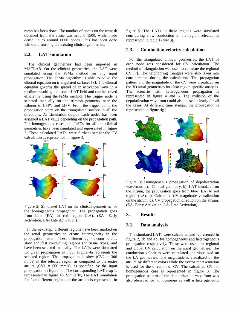
The clinical geometries had been imported in MATLAB. On the clinical geometries, the LAT were simulated using the FaMa method for any input propagation. The FaMa algorithm is able to solve the eikonal equation on triangulated surfaces [8]. The eikonal equation governs the spread of an activation wave in a medium resulting in a scalar LAT field and can be solved efficiently using the FaMa method. The trigger node is selected manually on the trimesh geometry near the isthmus of LSPV and LIPV. From the trigger point, the propagation starts on the triangulated surface in all the directions. As simulation output, each nodes has been assigned a LAT value depending on the propagation path. For homogeneous cases, the LATs for all the clinical geometries have been simulated and represented in figure 2. These calculated LATs, were further used for the CVcalculation as represented in figure 3.

Figure 2: Simulated LAT on the clinical geometries for the homogeneous propagation. The propagation goes from blue (EA) to red region (LA). (EA- Early Activation, LA- Late Activation).

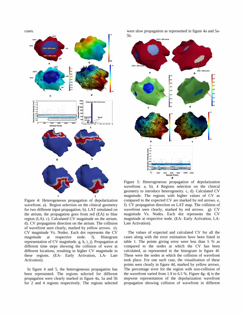
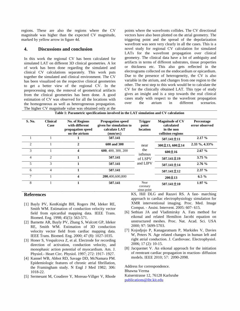
In the next step, different regions have been marked on the atrial geometries to create heterogeneity in the propagation pattern. These different regions contribute as slow and fast conducting regions (or tissue types) and have been selected manually. The LATs were simulated for given propagation as input. Figure 4a represents the selected region. The propagation is slow (CV2 = 300 mm/s) in the selected region as compared to the entire atrium (CV1 = 600 mm/s), as specified by the input propagation in figure 4a. The corresponding LAT map is represented in figure 4b. Similarly, The LAT simulation for four different regions on the atrium is represented in

figure 5. The LATs in these regions were simulated considering slow conduction in the region selected as represented in table 1 (row 3).

2.3. Conduction velocity calculation

For the triangulated clinical geometries, the LAT of each node was considered for CV calculation. The method of triangulation was used to calculate the regional CV [7]. The neighboring triangles were also taken into consideration during the calculation. The propagation pattern and the magnitude of the CV were visualized on the 3D atrial geometries for clear region-specific analysis. The scenario with heterogeneous propagation is represented in figure 4 and 5. The collision of the depolarization wavefront could also be seen clearly for all the cases. At different time stamps, the propagation is represented in figure 4g-j.

Figure 3: Homogeneous propagation of depolarization wavefront. a). Clinical geometry. b). LAT simulated on the atrium, the propagation goes from blue (EA) to red region (LA). c). Calculated CV magnitude visualization on the atrium. d). CV propagation direction on the atrium. (EA- Early Activation, LA- Late Activation).

3. Results

3.1. Data analysis

The simulated LATs were calculated and represented in figure 2, 3b and 4b, for homogeneous and heterogeneous propagation respectively. These were used for regional and global CV calculation on the atrial geometries. The conduction velocities were calculated and visualized on the LA geometries. The magnitude is visualized on the atrium by different colors while the vector representation is used for the direction of CV. The calculated CV for homogeneous case is represented in figure 3. The propagation pattern of the depolarization wavefront was also observed for homogeneous as well as heterogeneous

cases.

Figure 4: Heterogeneous propagation of depolarization wavefront. a). Region selection on the clinical geometry for two different input propagation. b). LAT simulated on the atrium, the propagation goes from red (EA) to blue region (LA). c). Calculated CV magnitude on the atrium. d). CV propagation direction on the atrium. The collision of wavefront seen clearly, marked by yellow arrows. e). CV magnitude Vs. Nodes. Each dot represents the CV magnitude at respective node. f). Histogram representation of CV magnitude. g, h, i, j). Propagation at different time steps showing the collision of wave at different locations, resulting in higher CV magnitude in these regions. (EA- Early Activation, LA- Late Activation).

In figure 4 and 5, the heterogeneous propagation has been represented. The regions selected for different propagation were clearly marked in figure 4a, 5a and 5b for 2 and 4 regions respectively. The regions selected

were slow propagation as represented in figure 4a and 5a- 5b.

Figure 5: Heterogeneous propagation of depolarization wavefront. a, b). 4 Regions selection on the clinical geometry to introduce heterogeneity. c, d). Calculated CV magnitude. The regions with higher values of CV as compared to the expected CV are marked by red arrows. e, f). CV propagation direction on LAT map. The collision of wavefront seen clearly, marked by red arrows. g). CV magnitude Vs. Nodes. Each dot represents the CV magnitude at respective node. (EA- Early Activation, LA- Late Activation).

The values of expected and calculated CV for all the cases along with the error estimation have been listed in table 1. The points giving error were less than 5 % as compared to the nodes at which the CV has been calculated, as represented in the histogram in figure 4f. These were the nodes at which the collision of wavefront took place. For one such case, the visualization of these points seen clearly in figure 4d, marked by yellow arrows. The percentage error for the region with non-collision of the wavefront varied from 1.9 to 6.5 %. Figure 4g- 4j is the stepwise representation of the depolarization wavefront propagation showing collision of wavefront in different

regions. These are also the regions where the CV magnitude was higher than the expected CV magnitude, marked by yellow arrow in figure 4d.

4. Discussions and conclusion

In this work the regional CV has been calculated for simulated LAT on different 3D clinical geometries. A lot of work has been done regarding the simulated and clinical CV calculations separately. This work puts together the simulated and clinical environment. The CV has been visualized on the respective clinical geometries to get a better view of the regional CV. In the preprocessing step, the removal of geometrical artifacts from the clinical geometries has been done. A good estimation of CV was observed for all the locations with the homogeneous as well as heterogeneous propagation. The higher CV magnitude value was obtained only at the

points where the wavefronts collides. The CV directional vectors have also been plotted on the atrial geometry. The triggering point and the spread of the depolarization wavefront was seen very clearly in all the cases. This is a novel study for regional CV calculation for simulated LATs for the wavefront propagation over clinical geometry. The clinical data have a lot of ambiguity and artifacts in terms of different substrates, tissue properties or thickness etc. This also gets reflected in the electrograms collected on the endocardium or epicardium. Due to the presence of heterogeneity, the CV is also variable in the atrium, and changes from one region to the other. The next step to this work would be to calculate the CV for the clinically obtained LAT. This type of study gives an insight and is a step towards the real clinical cases study with respect to the wavefront propagation over the atrium in different scenarios.

Table 1: Parametric specifications involved in the LAT simulation and CV calculation

S. No. Clinical Case

No. of Regions with different

propagation speed on the atrium

Propagation speed given for simulation to

calculate LAT (mm/sec)

Trigger point

location

Magnitude of CV calculated in the non

collision regions

Percentage error observed

1 1 1 507.141

near the

isthmus of LSPV and LIPV

507.141土11 2.17 %

2 1 2 600 and 300 300土13, 600土14 2.33 %, 4.33%

3 1 4 600, 400, 300, 200 600土16 2.67 %

4 2 1 507.141 507.141土19 3.75 %

5 3 1 507.141 507.141土14 2.76 %

6 4 1 507.141 507.141土12 2.37 %

7 1 4 200,400,600,800 200土13 6.5 %

8 1 1 507.141 Near coronary

sinus point

507.141土10 1.97 %

References

[1] Bayly PV, KenKnight BH, Rogers JM, Ideker RE, Smith WM. Estimation of conduction velocity vector field from epicardial mapping data. IEEE Trans. Biomed. Eng. 1998; 45(5): 563-571.

[2] Barnette AR, Bayly PV, Zhang S, Walcott GP, Ideker RE, Smith WM. Estimation of 3D conduction velocity vector field from cardiac mapping data. IEEE Trans. Biomed. Eng. 2000; 47 (8): 1027-1035.

[3] Honer S, Vespalcova Z, et al. Electrode for recording direction of activation, conduction velocity, and monophasic action potential of myocardium. Am. J. Physiol.- Heart Circ. Physiol. 1997; 272: 1917- 1927.

[4] Kannel WB, Abbot RD, Savage DD, McNamara PM. Epidemiologic features of chronic atrial fibrillation, the Framingham study. N Engl J Med 1982; 306: 1018-22.

[5] Sermesant M, Coudiere Y, Moreau-Villger V, Rhode

KS, Hill DLG and Razavi RS. A fast- marching approach to cardiac electrophysiology simulation for XMR interventional imaging. Proc. Med. Image Comput. - Assist. Intervent. 2005: 607- 615.

[6] Sethian JA and Vladimirsky A. Fats method for eikonal and related Hemilton Jacobi equation on unstructured meshes. Proc. Nat. Acad. Sci. USA 2000; 97: 5699-5703.

[7] Kojodjojo P, Kanagaratnam P, Markides V, Davies W, Peters N. Age related changes in human left and right atrial conduction. J. Cardiovasc. Electrophysiol. 2006; 17 (2): 10-15.

[8] Jacquemet V. An eikonal approach for the initiation of reentrant cardiac propagation in reaction- diffusion models. IEEE 2010; 57: 2090-2098.

Address for correspondence. Bhawna Verma Kaiserstrasse 12, 76128 Karlsruhe publications@ibt.kit.edu