Mathematical programming Linear programming problems Model ...

Reformulations in Mathematical Programming: AComputational Approach
Leo Liberti, Sonia Cafieri, and Fabien Tarissan
LIX, Ecole Polytechnique, Palaiseau, 91128 Franceliberti,cafieri,[email protected]
Summary. Mathematical programming is a language for describing optimization problems; it is based onparameters, decision variables, objective function(s) subject to various types of constraints. The presenttreatment is concerned with the case when objective(s) and constraints are algebraic mathematical expres-sions of the parameters and decision variables, and therefore excludes optimization of black-box functions.A reformulation of a mathematical program P is a mathematical program Q obtained from P via symbolictransformations applied to the sets of variables, objectives and constraints. We present a survey of existingreformulations interpreted along these lines, some example applications, and describe the implementationof a software framework for reformulation and optimization.
1 Introduction
Optimization and decision problems are usually defined by their input and a mathematical de-scription of the required output: a mathematical entity with an associated value, or whether agiven entity has a specified mathematical property or not. These mathematical entities and prop-erties are expressed in the language of set theory, most often in the ZFC axiomatic system [62].The scope of set theory language in ZFC is to describe all possible mathematical entities, and itslimits are given by Godel’s incompleteness theorem.
Optimization and decision problems are special in the sense that they are closely linked to aparticular algorithmic process designed to solve them: more precisely, although the algorithm isnot directly mentioned in the problem definition, the main reason why problems are formally castis that a solution to the problem is desired. In this respect the usual set theoretical language, withall its expressive powers, falls short of this requirement: specifically, no algorithm is so “generic”that it can solve all problems formulated in terms of set theory. Just to make an example, all LinearProgramming (LP) problems can be expressed in a language involving real numbers, variables, alinear form to be minimized, a system of linear equations to be satisfied, and a set of non-negativityconstraints on the variables. This particular language is not as expressive as the set-theoreticallanguage used in ZFC. On the other hand, there exists an algorithm, namely the simplex algorithm[26], which is generic enough to solve any LP problem, and which performs well in practice.
In its most general terms, a decision problem can be expressed as follows: given a set W and asubset D ⊆ W , decide whether a given x ∈ W belongs to D or not. Even supposing that W hasfinite cardinality (so that the problem is certainly decidable), the only algorithm which is genericenough to solve this problem is complete enumeration, which is rendered practically useless by itslow efficiency. Informally speaking, when discussing decidable problems and solution algorithms,there is a trade-off between how expressive is the language in which the problem is formulated,and how efficient is the associated solution algorithm.
Mathematical programming can be seen as a language which is powerful enough to expressalmost all practically interesting optimization and decision problems. Mathematical programmingformulations can be categorized according to various properties, and rather efficient solution algo-rithms exist for many of the categories. The semantic scope of mathematical programming is to

2 Leo Liberti, Sonia Cafieri, and Fabien Tarissan
define optimization and decision problems: as this scope is narrower than that of the set theoreti-cal language of ZFC, according to the trade-off principle mentioned above, the associated genericalgorithms are more efficient.
As in most languages, the same semantics can be conveyed by many different syntacticalexpressions. In other words, there are many equivalent formulations for each given problem (whatthe term “equivalent” means in this context will be defined later). Furthermore, solution algorithmsfor mathematical programming formulations often rely on solving a sequence of different problems(often termed auxiliary problems) related to the original one: although these are usually not fullyequivalent to the original problem, they may be relaxations, projections, liftings, decompositions(among others). The relations between the original and auxiliary problems are expressed in theliterature by means of logical, algebraic and/or transcendental expressions which draw on the samefamiliar ZFC language. As long as theoretical statements are being made, there is nothing wrongwith this, for people are usually able to understand that language. There is, however, a big gapbetween understanding the logical/algebraic relations among sets of optimization problems, andbeing able to implement algorithms using these problems in various algorithmic steps. Existingdata structures and code libraries usually offer numerical rather than symbolic manipulation tools.Symbolic algorithms and libraries exist, but they are not purpose-built to deal with optimizationand decision problems.
Consider for example the Kissing Number Problem (KNP) in D dimensions [60], i.e. the de-termination of the maximum number of unit D-dimensional spheres that can be arranged arounda central unit D-dimensional sphere. As all optimization problems, this can be cast (by using abisection argument) as a sequence of decision problems on the cardinality of the current spheresconfiguration. Namely, given the positive integers D (dimension of Euclidean space) and N , isthere a configuration of N unit spheres around the central one? For any fixed D, the answer willbe affirmative or negative depending on the value of N . The highest N such that the answer isaffirmative is the kissing number for dimension D. The decision version of the KNP can be castas a nonconvex Nonlinear Programming (NLP) feasibility problem as follows. For all i ≤ N , letxi = (xi1, . . . , xiD) ∈ RD be the center of the i-th sphere. We look for a set of vectors xi | i ≤ Nsatisfying the following constraints:
∀ i ≤ N ||xi|| = 2
∀ i < j ≤ N ||xi − xj || ≥ 2
∀ i ≤ N − 2 ≤ xi ≤ 2.
It turns out that this problem is numerically quite difficult to solve, as it is very unlikely that thelocal NLP solution algorithm will be able to compute a feasible starting solution. Failing to findan initial feasible solution means that the solver will immediately abort without having made anyprogress. Most researchers with some practical experience in NLP solvers (such as e.g. SNOPT[40]), however, will immediately reformulate this problem into a more computationally amenableform by squaring the norms to get rid of a potentially problematic square root, and treating thereverse convex constraints ||xi − xj || ≥ 2 as soft constraints by multiplying the right hand sidesby a non-negative scaling variable α, which is then maximized:
maxα (1)
∀ i ≤ N ||xi||2 = 4 (2)
∀ i < j ≤ N ||xi − xj ||2 ≥ 4α. (3)
∀ i ≤ N − 2 ≤ xi ≤ 2 (4)
α ≥ 0. (5)
In this form, finding an initial feasible solution is trivial; for example, xi = (2, 0, . . . , 0) for all i ≤ Nwill do. Subsequent solver iterations will likely be able to provide a better solution. Should thecomputed value of α be ≥ 1, the solution would be feasible in the hard constraints, too. Currently,we are aware of no optimization language environment that is able to perform the described

Reformulations in Mathematical Programming: A Computational Approach 3
reformulation automatically. Whilst this is not a huge limitation for NLP experts, people whosimply wish to model a problem and get its solution will fail to obtain one, and may even be ledinto thinking that the formulation itself is infeasible.
Another insightful example of the types of limitations we refer to can be drawn from the KNP.We might wish to impose ordering constraints on some of the spheres to reduce the number ofsymmetric solutions. Ordering spheres packed on a spherical surface is hard to do in Euclideancoordinates, but it can be done rather easily in spherical coordinates, by simply stating that thevalue of a spherical coordinate of the i-th sphere must be smaller than the corresponding value inthe j-th sphere. We can transform a Euclidean coordinate vector x = (x1, . . . , xD) in D-sphericalcoordinates (ρ, ϑ1, . . . , ϑD−1) such that ρ = ||x|| and ϑ ∈ [0, 2π]D−1 by means of the followingequations:
ρ = ||x|| (6)
∀k ≤ D xk = ρ sinϑk−1
D−1∏
h=k
cosϑh (7)
(this yields another NLP formulation of the KNP). Applying the D-spherical transformation issimply a matter of term rewriting and algebraic simplification, and yet no optimization languageenvironment offers such capabilities. By pushing things further, we might wish to devise an algo-rithm that dynamically inserts or removes constraints expressed in either Euclidean or sphericalcoordinates depending on the status of the current solution, and re-solves the (automatically) re-formulated problem at each iteration. This may currently be done (up to a point) by optimizationlanguage environments such as AMPL [38], provided all constraints are part of a pre-specifiedfamily of parametric constraints. Creating new constraints by term rewriting, however, is not atask that can currently be carried out automatically.
The limitations emphasized in the KNP example illustrate a practical need for very sophisti-cated software including numerical as well as symbolic algorithms, both applied to the unique goalof solving optimization problems cast as mathematical programming formulations. The currentstate of affairs is that there are many numerical optimization solvers and many Computer AlgebraSystems (CAS) — such as Maple or Mathematica — whose efficiency is severely hampered by thefull generality of their capabilities. In short, we would ideally need (small) parts of the symbolickernels driving the existing CASes to be combined with the existing optimization algorithms, plusa number of super-algorithms capable of making automated, dynamic decisions on the type ofreformulations that are needed to improve the current search process.
Although the above paradigm might seem far-fetched, it does in fact already exist in the formof the hugely successful CPLEX [51] solver targeted at solving Mixed-Integer Linear Program-ming (MINLP) problems. The initial formulation provided by the user is automatically simplifiedand improved with a sizable variety of pre-processing steps which attempt to reduce the numberof variables and constraints. Thereafter, at each node of the Branch-and-Bound algorithm, theformulation may be tightened as needed by inserting and removing additional valid constraints,in the hope that the current relaxed solution of the (automatically obtained) linear relaxation isimproved. Advanced users may of course decide to tune many parameters controlling this process,but practitioners needing a practical answer can simply use default parameters and to let CPLEXdecide what is best. Naturally, the task carried out by CPLEX is greatly simplified by the assump-tion that both objective function and constraints are linear forms, which is obviously not the casein a general nonlinear setting.
In this chapter we attempt to move some steps in the direction of endowing general mathemat-ical programming with the same degree of algorithmic automation enjoyed by linear programming.We propose: (a) a theoretical framework in which mathematical programming reformulations canbe formalized in a unified way, and (b) a literature review of the most successful existing refor-mulation and relaxation techniques in mathematical programming. Since an all-comprehensiveliterature review in reformulation techniques would extend this chapter to possibly several hun-dreds (thousands?) pages, only a partial review has been provided. In this sense, this should beseen as “work in progress” towards laying the foundations to a computer software which is capable
4 Leo Liberti, Sonia Cafieri, and Fabien Tarissan
of reformulating mathematical programming formulations automatically. Note also that for thisreason, the usual mathematical notations have been translated to a data structure frameworkthat is designed to facilitate computer implementation. Most importantly, “functions” — whichas mathematical entities are interpreted as maps between sets — are represented by expressiontrees: what is meant by the expression x+ y, for example, is really a directed binary tree on thevertices +, x, y with arcs (+, x), (+, y). For clarity purposes, however, we also provide theusual mathematical languages.
One last (but not least) remark is that reformulations can be seen as a new way of expressinga known problem. Reformulations are syntactical operations that may add or remove variables orconstraints, whilst keeping the fundamental structure of the problem optima invariant. When somenew variables are added and some of the old ones are removed, we can usually try to re-interpret thereformulated problem and assign a meaning to the new variables, thus gaining new insights to theproblem. One example of this is given in Sect. 3.5. One other area in mathematical programmingthat provides a similarly clear relationship between mathematical syntax and semantics is LPduality with the interpretation of reduced costs. This is important insofar as it offers alternativeinterpretations to known problems, which gains new and useful insights.
The rest of this chapter is organized as follows. In Section 2 we propose a general theoreticalframework of definitions allowing a unified formalization of mathematical programming reformu-lations. The definitions allow a consistent treatment of the most common variable and constraintmanipulations in mathematical programming formulations. In Section 3 we present a systematicstudy of a set of well known reformulations. Most reformulations are listed as symbolic algorithmsacting on the problem structure, although the equivalent transformation in mathematical termsis given for clarity purposes. In Section 4 we present a systematic study of a set of well knownrelaxations. Again, relaxations are listed as symbolic algorithms acting on the problem structurewhenever possible, the equivalent mathematical transformation being given for clarity. Section 5describes the implementation of ROSE, a Reformulation/Optimization Software Engine.
2 General framework
In Sect. 2.1 we formally define what a mathematical programming formulation is. In Sect. 2.2we discuss the expression tree function representation. Sect. 2.3 lists the most common standardforms in mathematical programming.
2.1 A data structure for mathematical programming formulations
In this chapter we give a formal definition of a mathematical programming formulation in suchterms that can be easily implemented on a computer. We then give several examples to illustratethe generality of our definition. We refer to a mathematical programming problem in the mostgeneral form:
min f(x)g(x) ⋚ bx ∈ X,
(8)
where f, g are function sequences of various sizes, b is an appropriately-sized real vector, and X isa cartesian product of continuous and discrete intervals.
The precise definition of a mathematical programming formulation lists the different formu-lation elements: parameters, variables having types and bounds, expressions depending on theparameters and variables, objective functions and constraints depending on the expressions. Welet P be the set of all mathematical programming formulations, and M be the set of all matrices.This is used in Defn. 1 to define leaf nodes in mathematical expression trees, so that the conceptof a formulation can also accommodate multilevel and semidefinite programming problems. No-tationwise, in a digraph (V,A) for all v ∈ V we indicate by δ+(v) the set of vertices u for which(v, u) ∈ A and by δ−(v) the set of vertices u for which (u, v) ∈ A.

Reformulations in Mathematical Programming: A Computational Approach 5
Definition 1. Given an alphabet L consisting of countably many alphanumeric names NL andoperator symbols OL, a mathematical programming formulation P is a 7-tuple (P,V, E ,O, C,B, T ),where:
• P ⊆ NL is the sequence of parameter symbols: each element p ∈ P is a parameter name;• V ⊆ NL is the sequence of variable symbols: each element v ∈ V is a variable name;• E is the set of expressions: each element e ∈ E is a Directed Acyclic Graph (DAG) e = (Ve, Ae)
such that:(a) Ve ⊆ L is a finite set(b) there is a unique vertex re ∈ Ve such that δ−(re) = ∅ (such a vertex is called the root vertex)(c) vertices v ∈ Ve such that δ+(v) = ∅ are called leaf vertices and their set is denoted by λ(e);
all leaf vertices v are such that v ∈ P ∪ V ∪ R ∪ P ∪M
(d) for all v ∈ Ve such that δ+(v) 6= ∅, v ∈ OL
(e) two weight functions χ, ξ : Ve → R are defined on Ve: χ(v) is the node coefficient and ξ(v)is the node exponent of the node v; for any vertex v ∈ Ve, we let τ(v) be the symbolic termof v: namely, v = χ(v)τ(v)ξ(v).
elements of E are sometimes called expression trees; nodes v ∈ OL represent an operation onthe nodes in δ+(v), denoted by v(δ+(v)), with output in R;
• O ⊆ −1, 1 × E is the sequence of objective functions; each objective function o ∈ O has theform (do, fo) where do ∈ −1, 1 is the optimization direction (−1 stands for minimization,+1 for maximization) and fo ∈ E;
• C ⊆ E × S × R (where S = −1, 0, 1) is the sequence of constraints c of the form (ec, sc, bc)with ec ∈ E , sc ∈ S, bc ∈ R:
c ≡
ec ≤ bc if sc = −1ec = bc if sc = 0ec ≥ bc if sc = 1;
• B ⊆ R|V| × R|V| is the sequence of variable bounds: for all v ∈ V let B(v) = [Lv, Uv] withLv, Uv ∈ R;
• T ⊆ 0, 1, 2|V| is the sequence of variable types: for all v ∈ V, v is called a continuous variableif T (v) = 0, an integer variable if T (v) = 1 and a binary variable if T (v) = 2.
We remark that for a sequence of variables z ⊆ V we write T (z) and respectively B(z) to meanthe corresponding sequences of types and respectively bound intervals of the variables in z. Givena formulation P = (P,V, E ,O, C,B, T ), the cardinality of P is |P | = |V|. We sometimes refer to aformulation by calling it an optimization problem or simply a problem.
Definition 2. Any formulation Q that can be obtained by P by a finite sequence of symbolicoperations carried out on the data structure is called a problem transformation.
Examples
In this section we provide some explicitly worked out examples that illustrate Defn. 1.
A quadratic problem
Consider the problem of minimizing the quadratic form 3x21+2x2
2+2x23+3x2
4+2x25+2x2
6−2x1x2−2x1x3 − 2x1x4 − 2x2x3 − 2x4x5 − 2x4x6 − 2x5x6 subject to x1 + x2 + x3 + x4 + x5 + x6 = 0 andxi ∈ −1, 1 for all i ≤ 6. For this problem,
• P = ∅;• V = (x1, x2, x3, x4, x5, x6);• E = (e1, e2) where e1, e2 are the graphs shown in Fig. 1;• O = (−1, e1);• C = ((e2, 0, 0));• B = ([−1, 1], [−1, 1], [−1, 1], [−1, 1], [−1, 1], [−1, 1]);• T = (2, 2, 2, 2, 2, 2).

6 Leo Liberti, Sonia Cafieri, and Fabien Tarissan
^ ^ ^ ^ ^ ^
+
××××××
×
×
×
×
×
×
×
×
×
×
×
×
×
×
33 2222
222222
−2−2−2−2−2−2−2
x1
x1x1x1 x2x2
x2
x3x3
x3
x4x4x4
x4
x5x5
x5
x6x6
x6
+
x1 x2 x3 x4 x5 x6
Fig. 1. The graphs e1 (above) and e2 (below) from Example 2.1.
Balanced graph bisection
Example 2.1 is a (scaled) mathematical programming formulation of a balanced graph bisectionproblem instance. This problem is defined as follows.
Balanced Graph Bisection Problem (BGBP). Given an undirected graph G = (V,E)without loops or parallel edges such that |V | is even, find a subset U ⊂ V such that
|U | = |V |2 and the set of edges C = u, v ∈ E | u ∈ U, v 6∈ U is as small as possible.
The problem instance considered in Example 2.1 is shown in Fig. 2. To all vertices i ∈ V we
associate variables xi =
1 i ∈ U−1 i 6∈ U
. The number of edges in C is counted by 14
∑
i,j∈E
(xi − xj)2.
The fact that |U | = |V |2 is expressed by requiring an equal number of variables at 1 and -1,
i.e.∑6
i=1 xi = 0.
1
2
3
4
5
6
Fig. 2. The BGBP instance in Example 2.1.
We can also express the problem in Example 2.1 as a particular case of the more generaloptimization problem:
minx x⊤Lx
s.t. x1 = 0x ∈ −1, 16,

Reformulations in Mathematical Programming: A Computational Approach 7
where
L =
3 −1 −1 −1 0 0−1 2 −1 0 0 0−1 −1 2 0 0 0−1 0 0 3 −1 −10 0 0 −1 2 −10 0 0 −1 −1 2
and 1 = (1, 1, 1, 1, 1, 1)⊤
. We represent this class of problems by the following mathematicalprogramming formulation:
• P = (Lij | 1 ≤ i, j ≤ 6);• V = (x1, x2, x3, x4, x5, x6);• E = (e′1, e2) where e′1 is shown in Fig. 3 and e2 is shown in Fig. 1 (below);• O = (−1, e′1);• C = ((e2, 0, 0));• B = ([−1, 1], [−1, 1], [−1, 1], [−1, 1], [−1, 1], [−1, 1]);• T = (2, 2, 2, 2, 2, 2).
^
2
^
2
^
2
^
2
^
2
^
2
+
××××××
×
×
×
×
×
×
×
×
×
×
×
×
×
×
L11 L22 L33 L44 L55 L66
L′12
L′13
L′14 L′
23L′
45 L′46 L′
56
x1
x1x1x1 x2x2
x2
x3x3
x3
x4x4x4
x4
x5x5
x5
x6x6
x6
Fig. 3. The graph e′1 from Example 2.1. L′
ij = Lij + Lji for all i, j.
The Kissing Number Problem
The kissing number problem formulation (1)-(5) is as follows:
• P = (N,D);• V = (xik | 1 ≤ i ≤ N ∧ 1 ≤ k ≤ D) ∪ α;• E = (f, hj , gij | 1 ≤ i < j ≤ N), where f is the expression tree for α, hj is the expression tree
for ||xj ||2 for all j ≤ N , and gij is the expression tree for ||xi − xj ||
2 − 4α for all i < j ≤ N ;• O = (1, f);• C = ((hi, 0, 4) | i ≤ N) ∪ ((gij , 1, 0) | i < j ≤ N);• B = [−2, 2]ND;• T = 0ND.

8 Leo Liberti, Sonia Cafieri, and Fabien Tarissan
As mentioned in Chapter 1, the kissing number problem is defined as follows.
Kissing Number Problem (KNP). Find the largest number N of non-overlapping unitspheres in RD that are adjacent to a given unit sphere.
The formulation of Example 2.1 refers to the decision version of the problem: given integers Nand D, is there an arrangement of N non-overlapping unit spheres in RD adjacent to a given unitsphere?
2.2 A data structure for mathematical expressions
Given an expression tree DAG e = (V,A) with root node r(e) and whose leaf nodes are elementsof R or of M (the set of all matrices), the evaluation of e is the (numerical) output of the operationrepresented by the operator in node r applied to all the subnodes of r (i.e. the nodes adjacent tor); in symbols, we denote the output of this operation by r(δ+(r)), where the symbol r denotesboth a function and a node. Naturally, the arguments of the operator must be consistent with theoperator meaning. We remark that for leaf nodes belonging to P (the set of all formulations), theevaluation is not defined; the problem in the leaf node must first be solved and a relevant optimalvalue (e.g. an optimal variable value, as is the case with multilevel programming problems) mustreplace the leaf node.
For any e ∈ E, the evaluation tree of e is a DAG e = (V , A) where V = v ∈ V | |δ+(v)| >0 ∨ v ∈ R ∪ x(v) | |δ+(v)| = 0 ∧ v ∈ V (in short, the same as V with every variable leaf nodereplaced by the corresponding value x(v)). Evaluation trees are evaluated by Alg. 1. We can nownaturally extend the definition of evaluation of e at a point x to expression trees whose leaf nodesare either in V or R.
Definition 3. Given an expression e ∈ E with root node r and a point x, the evaluation e(x) ofe at x is the evaluation r(δ+(r)) of the evaluation tree e.
Algorithm 1 The evaluation algorithm for expression trees.
double Eval(node v) double ρ;if (v ∈ OL)
// v is an operatorarray α[|δ+(v)|];∀ u ∈ δ+(v)
α(u) =Eval(u);ρ = χ(v)v(α)ξ(v);
else // v is a constant valueρ = χ(v)vξ(v);
return ρ;
We consider a sufficiently rich operator set OL including at least +,×, power, exponential,logarithm, and trigonometric functions (for real arguments) and inner product (for matrix argu-ments). Note that since any term t is weighted by a multiplier coefficient χ(t) there is no need toemploy a − operator, for it suffices to multiply χ(t) by −1 = ξ(v) in the appropriate term(s) t; adivision u/v is expressed by multiplying u by v raised to the power −1. Depending on the problemform, it may sometimes be useful to enrich OL with other (more complex) terms. In general, weview an operator in OL as an atomic operation on a set of variables with cardinality at least 1.

Reformulations in Mathematical Programming: A Computational Approach 9
A standard form for expressions
Since in general there is more than one way to write a mathematical expression, it is useful toadopt a standard form; whilst this does not resolve all ambiguities, it nonetheless facilitates thetask of writing symbolic computation algorithms acting on the expression trees. For any expressionnode t in an expression tree e = (V,A):
• if t is a sum:1. |δ+(t)| ≥ 22. no subnode of t may be a sum (sum associativity);3. no pair of subnodes u, v ∈ δ+(t) must be such that τ(u) = τ(v) (i.e. like terms must be
collected); as a consequence, each sum only has one monomial term for each monomial type4. a natural (partial) order is defined on δ+(t): for u, v ∈ δ+(t), if u, v are monomials, u, v are
ordered by degree and lexicographically• if t is a product:
1. |δ+(t)| ≥ 22. no subnode of t may be a product (product associativity);3. no pair of subnodes u, v ∈ δ+(t) must be such that τ(u) = τ(v) (i.e. like terms must be
collected and expressed as a power)• if t is a power:
1. |δ+(t)| = 22. the exponent may not be a constant (constant exponents are expressed by setting the
exponent coefficient ξ(t) of a term t)3. the natural order on δ+(t) lists the base first and the exponent later.
The usual mathematical nomenclature (linear forms, polynomials, and so on) applies to ex-pression trees.
2.3 Standard forms in mathematical programming
Solution algorithms for mathematical programming problems read a formulation as input andattempt to compute an optimal feasible solution as output. Naturally, algorithms which exploitproblem structure are usually more efficient than those that do not. In order to be able to exploitthe structure of the problem, solution algorithms solve problems that are cast in a standard formthat emphasizes the useful structure. In this section we review the most common standard forms.
Linear Programming
A mathematical programming problem P is a Linear Programming (LP) problem if (a) |O| = 1(i.e. the problem only has a single objective function); (b) e is a linear form for all e ∈ E ; and (c)T (v) = 0 (i.e. v is a continuous variable) for all v ∈ V.
An LP is in standard form if (a) sc = 0 for all constraints c ∈ C (i.e. all constraints are equalityconstraints) and (b) B(v) = [0,+∞] for all v ∈ V. LPs are expressed in standard form whenevera solution is computed by means of the simplex method [26]. By contrast, if all constraints areinequality constraints, the LP is known to be in canonical form.
Mixed Integer Linear Programming
A mathematical programming problem P is a Mixed Integer Linear Programming (MILP) problemif (a) |O| = 1; and (b) e is a linear form for all e ∈ E .
A MILP is in standard form if sc = 0 for all constraints c ∈ C and if B(v) = [0,+∞] for allv ∈ V. The most common solution algorithms employed for solving MILPs are Branch-and-Bound(BB) type algorithms [51]. These algorithms rely on recursively partitioning the search domain ina tree-like fashion, and evaluating lower and upper bounds at each search tree node to attempt to
10 Leo Liberti, Sonia Cafieri, and Fabien Tarissan
implicitly exclude some subdomains from consideration. BB algorithms usually employ the simplexmethod as a sub-algorithm acting on an auxiliary problem, so they enforce the same standard formon MILPs as for LPs. As for LPs, a MILP where all constraints are inequalities is in canonicalform.
Nonlinear Programming
A mathematical programming problem P is a Nonlinear Programming (NLP) problem if (a)|O| = 1 and (b) T (v) = 0 for all v ∈ V.
Many fundamentally different solution algorithms are available for locally solving NLPs, andmost of them require different standard forms. One of the most widely used is Sequential QuadraticProgramming (SQP) [40], which requires problem constraints c ∈ C to be expressed in the formlc ≤ c ≤ uc with lc, uc ∈ R ∪ −∞,+∞. More precisely, an NLP is in SQP standard form if forall c ∈ C (a) sc 6= 0 and (b) there is c′ ∈ C such that ec = ec′ and sc = −sc′ .
Mixed Integer Nonlinear Programming
A mathematical programming problem P is a Mixed Integer Nonlinear Programming (MINLP)problem if |O| = 1. The situation as regards MINLP standard forms is generally the same asfor NLPs, save that a few more works have appeared in the literature about standard forms forMINLPs [114, 115, 96, 72]. In particular, the Smith standard form [115] is purposefully constructedso as to make symbolic manipulation algorithms easy to carry out on the formulation. A MINLPis in Smith standard form if:
• O = do, eo where eo is a linear form;• C can be partitioned into two sets of constraints C1, C2 such that c is a linear form for all c ∈ C1
and c = (ec, 0, 0) for c ∈ C2 where ec is as follows:1. r(ec) is the sum operator2. δ+(r(ec)) = ⊗, v where (a) ⊗ is a nonlinear operator where all subnodes are leaf nodes,
(b) χ(v) = −1 and (c) τ(v) ∈ V.
Essentially, the Smith standard form consists of a linear part comprising objective functions and aset of constraints; the rest of the constraints have a special form ⊗(x1, . . . , xp)−v = 0 for some p ∈N, with v, x1, . . . , xp ∈ V(P ) and ⊗ a nonlinear operator in OL. By grouping all nonlinearities in aset of equality constraints of the form “variable = operator(variables)” (called defining constraints)the Smith standard form makes it easy to construct auxiliary problems. The Smith standard formcan be constructed by recursing on the expression trees of a given MINLP [113] and is an opt-reformulation.
Solution algorithms for solving MINLPs are usually extensions of BB type algorithms [115, 72,69, 125, 95].
Separable problems
A problem P is in separable form if (a) O(P ) = (do, eo), (b) C(P ) = ∅ and (c) eo is such that:
• r(eo) is the sum operator• for all distinct u, v ∈ δ+(r(eo)), λ(u) ∩ λ(v) = ∅,
where by slight abuse of notation λ(u) is the set of leaf nodes of the subgraph of eo whoseroot is u. The separable form is a standard form by itself. It is useful because it allows a veryeasy problem decomposition: for all u ∈ δ+(r(eo)) it suffices to solve the smaller problems Qu
with V(Qu) = λ(v) ∩ V(P ), O(Qu) = (do, u) and B(Qu) = B(P )(v) | v ∈ V(Qu). Then⋃
u∈δ+(r(eo))
x(V(Qu)) is a solution for P .

Reformulations in Mathematical Programming: A Computational Approach 11
Factorable problems
A problem P is in factorable form [91, 131, 112, 125] if:
1. O = (do, eo)2. r(eo) ∈ V (consequently, the vertex set of eo is simply r(eo))3. for all c ∈ C:• sc = 0• r(ec) is the sum operator• for all t ∈ δ+(r(ec)), either (a) t is a unary operator and δ+(t) ⊆ λ(ec) (i.e. the only
subnode of t is a leaf node) or (b) t is a product operator such that for all v ∈ δ+(t), v isa unary operator with only one leaf subnode.
The factorable form is a standard form by itself. Factorable forms are useful because it is easyto construct many auxiliary problems (including convex relaxations, [91, 3, 112]) from problemscast in this form. In particular, factorable problems can be reformulated to emphasize separability[91, 125, 95].
D.C. problems
The acronym “d.c.” stands for “difference of convex”. Given a set Ω ⊆ Rn, a function f : Ω → R isa d.c. function if it is a difference of convex functions, i.e. there exist convex functions g, h : Ω → R
such that, for all x ∈ Ω, we have f(x) = g(x)− h(x). Let C,D be convex sets; then the set C\Dis a d.c. set. An optimization problem is d.c. if the objective function is d.c. and Ω is a d.c. set. Inmost of the d.c. literature, however [130, 117, 49], a mathematical programming problem is d.c. if:
• O = (do, eo);• eo is a d.c. function;• c is a linear form for all c ∈ C.
D.C. programming problems have two fundamental properties. The first is that the space ofall d.c. functions is dense in the space of all continuous functions. This implies that any continu-ous optimization problem can be approximated as closely as desired, in the uniform convergencetopology, by a d.c. optimization problem [130, 49]. The second property is that it is possible togive explicit necessary and sufficient global optimality conditions for certain types of d.c. prob-lems [130, 117]. Some formulations of these global optimality conditions [116] also exhibit a veryuseful algorithmic property: if at a feasible point x the optimality conditions do not hold, thenthe optimality conditions themselves can be used to construct an improved feasible point x′.
Linear Complementarity problems
Linear complementarity problems (LCP) are nonlinear feasibility problems with only one nonlinearconstraint. An LCP is defined as follows [29], p. 50:
• O = ∅;• there is a constraint c′ = (e, 0, 0) ∈ C such that (a) t = r(e) is a sum operator; (b) for all
u ∈ δ+(t), u is a product of two terms v, f such that v ∈ V and (f, 1, 0) ∈ C;• for all c ∈ C r c′, ec is a linear form.
Essentially, an LCP is a feasibility problem of the form:
Ax ≥ bx ≥ 0
x⊤(Ax− b) = 0,
where x ∈ Rn, A is an m× n matrix and b ∈ Rm.Many types of mathematical programming problems (including MILPs with binary variables
[29, 53]) can be recast as LCPs or extensions of LCP problems [53]. Furthermore, some types ofLCPs can be reformulated to LPs [86] and as separable bilinear programs [87]. Certain types ofLCPs can be solved by an interior point method [58, 29].
12 Leo Liberti, Sonia Cafieri, and Fabien Tarissan
Bilevel Programming problems
The bilevel programming (BLP) problem consists of two nested mathematical programmingproblems named the leader and the follower problem.
A mathematical programming problem P is a bilevel programming problem if there exist twoprogramming problems L,F (the leader and follower problem) and a subset ℓ 6= ∅ of all leaf nodesof E(L) such that any leaf node v ∈ ℓ has the form (v,F) where v ∈ V(F ).
The usual mathematical notation is as follows [31, 12]:
miny F (x(y), y)minx f(x, y)
s.t. x ∈ X, y ∈ Y,
(9)
where X,Y are arbitrary sets. This type of problem arises in economic applications. The leaderknows the cost function of the follower, who may or may not know that of the leader; but thefollower knows the optimal strategy selected by the leader (i.e. the optimal values of the decisionvariables of L) and takes this into account to compute his/her own optimal strategy.
BLPs can be reformulated exactly to MILPs with binary variables and vice-versa [12], wherethe reformulation is as in Defn. 6. Furthermore, two typical Branch-and-Bound (BB) algorithmsfor the considered MILPs and BLPs have the property that the the MILP BB can be “embedded”in the BLP BB (this roughly means that the BB tree of the MILP is a subtree of the BB tree ofthe BLP); however, the contrary does not hold. This seems to hint at a practical solution difficultyranking in problems with the same degree of worst-case complexity (both MILPs and BLPs areNP-hard).
Semidefinite Programming problems
Consider known symmetric n×n matrices C,Ak for k ≤ m, a vector b ∈ Rm and a symmetric n×nmatrix X = (xij) where xij is a problem variable for all i, j ≤ n. The following is a semidefiniteprogramming problem (SDP) in primal form:
minX C •X∀k ≤ m Ak •X = bk
X 0,
(10)
where X 0 is a constraint that indicates that X should be symmetric positive semidefinite, andC •X = tr(C⊤X) =
∑
i,j cijxij . We also consider the SDP in dual form:
maxy,S b⊤y∑
k≤m ykAk + S = C
S 0,
(11)
where S is a symmetric n × n matrix and y ∈ Rm. Both forms of the SDP problem are convexNLPs, so the duality gap is zero. Both forms can be solved by a particular type of polynomial-timeinterior point method (IPM), which means that solving SDPs is practically efficient [7, 126]. SDPsare important because they provide tight relaxations to (nonconvex) quadratically constrainedquadratic programming problems (QCQP), i.e. problems with a quadratic objective and quadraticconstraints (see Sect. 4.3).
SDPs can be easily modelled with the data structure described in Defn. 1, for their expressiontrees are linear forms where each leaf node contains a symmetric matrix. There is no need toexplicitly write the semidefinite constraints X 0, S 0 because the solution IPM algorithmswill automatically find optimal X,S matrices that are semidefinite.

Reformulations in Mathematical Programming: A Computational Approach 13
3 Reformulations
In this section we define some types of reformulations and establish some links between them(Sect. 3.1) and we give a systematic study of various types of elementary reformulations (Sect. 3.2)and exact linearizations (Sect. 3.3). Sect. 3.5 provides a few worked out examples. In this summary,we tried to focus on two types of reformulations: those that are in the literature, but may not beknown to every optimization practitioner, and those that represent the “tricks of the trade” ofmost optimization researchers but have never, or rarely, been formalized explicitly; so the maincontributions of this section are systematic and didactic. Since the final aim of automatic refor-mulations is let the computer arrive at an alternative formulation which is easier to solve, weconcentrated on those reformulations which simplified nonlinear terms into linear terms, or whichreduced integer variables to continuous variables. By contrast, we did not cite important refor-mulations (such as the LP duality) which are fundamental in solution algorithms and alternativeproblem interpretation, but which do not significantly alter solution difficulty.
3.1 Reformulation definitions
Consider a mathematical programming formulation P = (P,V, E ,O, C,B, T ) and a function x :V → R|V| (called point) which assigns values to the variables.
Definition 4. A point x is type feasible if:
x(v) ∈
R if T (v) = 0Z if T (v) = 1Lv, Uv if T (v) = 2
for all v ∈ V; x is bound feasible if x(v) ∈ B(v) for all v ∈ V; x is constraint feasible if for allc ∈ C we have: ec(x) ≤ bc if sc = −1, ec(x) = bc if sc = 0, and ec(x) ≥ bc if sc = 1. A point x isfeasible in P if it is type, bound and constraint feasible.
A point x feasible in P is also called a feasible solution of P . A point which is not feasible is calledinfeasible. Denote by F(P ) the feasible points of P .
Definition 5. A feasible point x is a local optimum of P with respect to the objective o ∈ O ifthere is a non-empty neighbourhood N of x such that for all feasible points y 6= x in N we havedofo(x) ≥ dofo(y). A local optimum is strict if dofo(x) > dofo(y). A feasible point x is a globaloptimum of P with respect to the objective o ∈ O if dofo(x) ≥ dofo(y) for all feasible points y 6= x.A global optimum is strict if dofo(x) > dofo(y).
Denote the set of local optima of P by L(P ) and the set of global optima of P by G(P ). IfO(P ) = ∅, we define L(P ) = G(P ) = F(P ).
Example 1. The point x = (−1,−1,−1, 1, 1, 1) is a strict global minimum of the problem in Ex-ample 2.1 and |G| = 1 as U = 1, 2, 3 and V r U = 4, 5, 6 is the only balanced partition of Vleading to a cutset size of 1.
It appears from the existing literature that the term “reformulation” is almost never formallydefined in the context of mathematical programming. The general consensus seems to be thatgiven a formulation of an optimization problem, a reformulation is a different formulation havingthe same set of optima. Various authors make use of this definition without actually making itexplicit, among which [108, 115, 101, 81, 33, 43, 19, 98, 53, 29]. Many of the proposed reformula-tions, however, stretch this implicit definition somewhat. Liftings, for example (which consist inadding variables to the problem formulation), usually yield reformulations where an optimum inthe original problem is mapped to a set of optima in the reformulated problem (see Sect. 3.2).Furthermore, it is sometimes noted how a reformulation in this sense is overkill because the refor-mulation only needs to hold at global optimality [1]. Furthermore, reformulations sometimes really
14 Leo Liberti, Sonia Cafieri, and Fabien Tarissan
refer to a change of variables, as is the case in [93]. Throughout the rest of this section we givevarious definitions for the concept of reformulation, and we explore the relations between them.We consider two problems
P = (P(P ),V(P ), E(P ),O(P ), C(P ),B(P ), T (P ))
Q = (P(Q),V(Q), E(Q),O(Q), C(Q),B(Q), T (Q)).
Reformulations have been formally defined in the context of optimization problems (whichare defined as decision problems with an added objective function). As was noted in Sect. 1, wesee mathematical programming as a language used to describe and eventually solve optimizationproblems, so the difference is slim. The following definition is found in [12].
Definition 6. Let PA and PB be two optimization problems. A reformulation B(·) of PA as PB
is a mapping from PA to PB such that, given any instance A of PA and an optimal solution ofB(A), an optimal solution of A can be obtained within a polynomial amount of time.
This definition is directly inspired to complexity theory and NP-completeness proofs. In the morepractical and implementation oriented context of this chapter, Defn. 6 has one weak point, namelythat of polynomial time. In practice, depending on the problem and on the instance, a polynomialtime reformulation may just be too slow; on the other hand, Defn. 6 may bar a non-polynomialtime reformulation which might be actually carried out within a practically reasonable amountof time. Furthermore, a reformulation in the sense of Defn. 6 does not necessarily preserve localoptimality or the number of global optima, which might in some cases be a desirable reformulationfeature. It should be mentioned that Defn. 6 was proposed in a paper that was more theoretical innature, using an algorithmic equivalence between problems in order to attempt to rank equivalentNP-hard problems by their Branch-and-Bound solution difficulty.
The following definition was proposed by H. Sherali [105].
Definition 7. A problem Q is a reformulation of P if:
• there is a bijection σ : F(P )→ F(Q);• |O(P )| = |O(Q)|;• for all p = (ep, dp) ∈ O(P ), there is a q = (eq, dq) ∈ O(Q) such that eq = f(ep) where f is a
monotonic univariate function.
Defn. 7 imposes a very strict condition, namely the bijection between feasible regions of theoriginal and reformulated problems. Although this is too strict for many useful transformationsto be classified as reformulations, under some regularity conditions on σ it presents some addedbenefits, such as e.g. allowing easy correspondences between partitioned subspaces of the feasibleregions and mapping sensitivity analysis results from reformulated to original problem.
In the rest of the section we discuss alternative definitions which only make use of the conceptof optimum (also see [74]). These encompass a larger range of transformations as they do notrequire a bijection between the feasible regions, the way Defn. 7 does.
Definition 8. Q is a local reformulation of P if there is a function ϕ : F(Q) → F(P ) such that(a) ϕ(y) ∈ L(P ) for all y ∈ L(Q), (b) ϕ restricted to L(Q) is surjective. This relation is denotedby P ≺ϕ Q.
Informally, a local reformulation transforms all (local) optima of the original problem into optimaof the reformulated problem, although more than one reformulated optimum may correspond tothe same original optimum. A local reformulation does not lose any local optimality informationand makes it possible to map reformulated optima back to the original ones; on the other hand,a local reformulation does not keep track of globality: some global optima in the original problemmay be mapped to local optima in the reformulated problem, or vice-versa (see Example 2).
Example 2. Consider the problem P ≡ minx∈[−2π,2π]
x+ sin(x) and Q ≡ minx∈[−2π,2π]
sin(x). It is easy to
verify that there is a bijection between the local optima of P and those of Q. However, althoughP has a unique global optimum, every local optimum in Q is global.

Reformulations in Mathematical Programming: A Computational Approach 15
Definition 9. Q is a global reformulation of P if there is a function ϕ : F(Q)→ F(P ) such that(a) ϕ(y) ∈ G(P ) for all y ∈ G(Q), (b) ϕ restricted to G(Q) is surjective. This relation is denotedby P ϕ Q.
Informally, a global reformulation transforms all global optima of the original problem into globaloptima of the reformulated problem, although more than one reformulated global optimum maycorrespond to the same original global optimum. Global reformulations are desirable, in the sensethat they make it possible to retain the useful information about the global optima whilst ignoringlocal optimality. At best, given a difficult problem P with many local minima, we would like tofind a global reformulation Q where L(Q) = G(Q).
Example 3. Consider a problem P with O(P ) = f. Let Q be a problem such that O(Q) = f
and F(Q) = conv(F(P )), where conv(F(P )) is the convex hull of the points of F(P ) and f is
the convex envelope of f over the convex hull of F(P ) (in other words, f is the greatest convexfunction underestimating f on F(P )). Since the set of global optima of P is contained in the setof global optima of Q [48], the convex envelope is a global reformulation.
Unfortunately, finding convex envelopes in explicit form is not easy. A considerable amount ofwork exists in this area: e.g. for bilinear terms [91, 6], trilinear terms [92], fractional terms [123],monomials of odd degree [80, 67] the envelope is known in explicit form (this list is not exhaustive).See [120] for recent theoretical results and a rich bibliography.
Definition 10. Q is an opt-reformulation (or exact reformulation) of P (denoted by P < Q) ifthere is a function ϕ : F(Q)→ F(P ) such that P ≺ϕ Q and P ϕ Q.
This type of reformulation preserves both local and global optimality information, which makes itvery attractive. Even so, Defn. 10 fails to encompass those problem transformations that eliminatesome global optima whilst ensuring that at least one global optimum is left. Such transformationsare specially useful in Integer Programming problems having several symmetric optimal solutions:restricting the set of global optima in such cases may be beneficial. One such example is thepruning of Branch-and-Bound regions based on the symmetry group of the problem presented in[89]: the set of cuts generated by the procedure fails in general to be a global reformulation in thesense of Defn. 9 because the number of global optima in the reformulated problem is smaller thanthat of the original problem.
Lemma 1. The relations ≺,, < are reflexive and transitive, but in general not symmetric.
Proof. For reflexivity, simply take ϕ as the identity. For transitivity, let P ≺ Q ≺ R with functionsϕ : F(Q)→ F(P ) and ψ : F(R)→ F(Q). Then ϑ = ϕ ψ has the desired properties. In order toshow that ≺ is not symmetric, consider a problem P with variables x and a unique minimum x∗
and a problem Q which is exactly like P but has one added variable w ∈ [0, 1]. It is easy to showthat P ≺ Q (take ϕ as the projection of (x,w) on x). However, since for all w ∈ [0, 1] (x∗, w) is anoptimum of Q, there is no function of a singleton to a continuously infinite set that is surjective,so Q 6≺ P .
Given a pair of problems P,Q where ≺,, < are symmetric on the pair, we call Q a symmetricreformulation of P . We remark also that by Lemma (1) we can compose elementary reformulationstogether to create chained reformulations (see Sect. 3.5 for examples).
Definition 11. Any problem Q that is related to a given problem P by a formula f(Q,P ) = 0where f is a computable function is called an auxiliary problem with respect to P .
Deriving the formulation of an auxiliary problem may be a hard task, depending on f . The mostuseful auxiliary problems are those whose formulation can be derived algorithmically in timepolynomial in |P |.
We remark that casting a problem in a standard form is an opt-reformulation. A good reformu-lation framework should be aware of the available solution algorithms and attempt to reformulategiven problems into the most appropriate standard form.

16 Leo Liberti, Sonia Cafieri, and Fabien Tarissan
3.2 Elementary reformulations
In this section we introduce some elementary reformulations in the proposed framework.
Objective function direction
Given an optimization problem P , the optimization direction do of any objective function o ∈ O(P )can be changed by simply setting do ← −do. This is an opt-reformulation where ϕ is the identity,and it rests on the identity min f(x) = −max−f(x). We denote the effect of this reformulationcarried out on each objective of a set O ⊆ O by ObjDir(P,O).
Constraint sense
Changing constraint sense simply means to write a constraint c expressed as ec ≤ bc as −ec ≥ −bc,or ec ≥ bc as −ec ≤ −bc. This is sometimes useful to convert the problem formulation to a givenstandard form. This is an opt-reformulation where ϕ is the identity. It can be carried out on theformulation by setting χ(r(ec))← −χ(r(ec)), sc ← −sc and bc = −bc. We denote the effect of thisreformulation carried out for all constraints in a given set C ⊆ C by ConSense(P,C).
Liftings, restrictions and projections
We define here three important classes of auxiliary problems: liftings, restrictions and projections.Essentially, a lifting is the same as the original problem but with more variables. A restriction isthe same as the original problem but with some of the variables replaced by either parameters orconstants. A projection is the same as the original problem projected onto fewer variables. Whereasit is possible to give definitions of liftings and restrictions in terms of symbolic manipulations tothe data structure given in Defn. 1, such a definition is in general not possible for projections.Projections and restrictions are in general not opt-reformulations nor reformulations in the senseof Defn. 7.
Lifting
A lifting Q of a problem P is a problem such that: P(Q) ) P(P ), V(Q) ) V(P ), O(Q) = O(P ),E(Q) ) E(P ), C(Q) = C(P ), B(Q) ) B(P ), T (Q) ) T (P ). This is an opt-reformulation where ϕis a projection operator from V(Q) onto V(P ): for y ∈ F(Q), let ϕ(y) = (y(v) | v ∈ V(P )). Wedenote the lifting with respect to a new set of variables V by Lift(P, V ).
Essentially, a lifting is obtained by adding new variables to an optimization problem.
Restriction
A restriction Q of a problem P is such that:
• P(Q) ⊇ P(P )• V(Q) ( V(P )• |O(Q)| = |O(P )|• |C(Q)| = |C(P )|• for each e ∈ E(P ) there is e′ ∈ E(Q) such that e′ is the same as e with any leaf node v ∈V(P ) r V(Q) replaced by an element of P(Q) ∪ R.
We denote the restriction with respect to a sequence of variable V with a corresponding sequenceof values R by Restrict(P, V,R).
Essentially, a restriction is obtained by fixing some variables at corresponding given values.

Reformulations in Mathematical Programming: A Computational Approach 17
Projection
A projection Q of a problem P is such that:
• P(Q) ⊇ P(P )• V(Q) ( V(P )• E ,O, C,B, T (Q) are so that for all y ∈ F(Q) there is x ∈ F(P ) such that x(v) = y(v) for all
v ∈ V(Q).
In general, symbolic algorithms to derive projections depend largely on the structure of the expres-sion trees in E. If E consists entirely of linear forms, this is not difficult (see e.g. [14], Thm. 1.1).We denote the projection onto a set of variables V = V(Q) as Proj(P, V ).
Essentially, F(Q) = y | ∃x (x, y) ∈ F(P ).
Equations to inequalities
Converting equality constraints to inequalities may be useful to conform to a given standard form.Suppose P has an equality constraint c = (ec, 0, bc). This can be reformulated to a problem Q asfollows:
• add two constraints c1 = (ec,−1, bc) and c2 = (ec, 1, bc) to C;• remove c from C.
This is an opt-reformulation denoted by Eq2Ineq(P, c).Essentially, we replace the constraint ec = bc by the two constraints ec ≤ bc, ec ≥ bc.
Inequalities to equations
Converting inequalities to equality constraints is useful to convert problems to a given standardform: a very well known case is the standard form of a Linear Programming problem for use withthe simplex method. Given a constraint c expressed as ec ≤ bc, we can transform it into an equalityconstraint by means of a lifting operation and a simple symbolic manipulation on the expressiontree ec, namely:
• add a variable vc to V(P ) with interval bounds B(vc) = [0,+∞] (added to B(P )) and typeT (vc) = 0 (added to T (P ));
• add a new root node r0 corresponding to the operator + (sum) to ec = (V,A), two arcs(r0, r(ec)), (r0, v) to A, and we then set r(ec)← r0;
• set sc ← 0.
We denote this transformation carried out on the set of constraints C by Slack(P,C). Naturally,for original equality constraints, this transformation is defined as the identity.
Performing this transformation on any number of inequality constraints results into an opt-reformulation.
Proposition 1. Given a set of constraints C ⊆ C(P ), the problem Q = Slack(P,C) is an opt-reformulation of P .
Proof. We first remark that V(P ) ⊆ V(Q). Consider ϕ defined as follows: for each y ∈ F(Q) letϕ(y) = x = (y(v) | v ∈ V(P )). It is then easy to show that ϕ satisfies Defn. 10.
Absolute value terms
Consider a problem P involving a term e = (V,A) ∈ E where r(e) is the absolute value operator| · | (which is continuous but not differentiable everywhere); since this operator is unary, there isa single expression node f such that (r(e), f) ∈ A. This term can be reformulated so that it isdifferentiable, as follows:

18 Leo Liberti, Sonia Cafieri, and Fabien Tarissan
• add two continuous variables t+, t− with bounds [0,+∞];• replace e by t+ + t−;• add constraints (f − t+ − t−, 0, 0) and (t+t−, 0, 0) to C.
This is an opt-reformulation denoted by AbsDiff(P, e).Essentially, we replace all terms |f | in the problem by a sum t+ + t−, and then add the
constraints f = t+ + t− and t+t− = 0 to the problem.
Product of exponential terms
Consider a problem P involving a product g =∏
i≤k hi of exponential terms, where hi = efi forall i ≤ k. This term can be reformulated as follows:
• add a continuous variable w to V with T (w) = 0 and bounds B(w) = [0,+∞];• add a constraint c = (ec, 0, 0) where ec =
∑
i≤k fi − log(w) to C;• replace g with w.
This is an opt-reformulation denoted by ProdExp(P, g). It is useful because many nonlinear terms(product and exponentials) have been the reduced to only one (the logarithm).
Essentially, we replace the product∏
i efi by an added nonnegative continuous variable w and
then add the constraint log(w) =∑
i fi to the problem.
Binary to continuous variables
Consider a problem P involving a binary variable x ∈ V with (T (x) = 2). This can be reformulatedas follows:
• add a constraint c = (ec, 0, 0) to C where ec = x2 − x;• set T (x) = 0.
This is an opt-reformulation denoted by Bin2Cont(P, x). Since a binary variable x ∈ V can onlytake values in 0, 1, any univariate equation in x that has exactly x = 0 and x = 1 as solutionscan replace the binary constraint x ∈ 0, 1. The most commonly used is the quadratic constraintx2 = x, sometimes also written as x(x− 1) ≥ 0 ∧ x ≤ 1 [119].
In principle, this would reduce all binary problems to nonconvex quadratically constrainedproblems, which can be solved by a global optimization (GO) solver for nonconvex NLPs. Inpractice, GO solvers rely on an NLP subsolver to do most of the computationally intensive work,and NLP solvers are generally not very good in handling nonconvex/nonlinear equality constraintssuch as x2 = x. This reformulation, however, is often used in conjunction with the relaxation ofbinary linear and quadratic problems (see Sect. 4.4).
Integer to binary variables
It is sometimes useful, for different reasons, to convert general integer variables to binary (0-1)variables. One example where this yields a crucial step into a complex linearization is given inSect. 3.5. There are two established ways of doing this: one entails introducing binary assignmentvariables for each integer values that the variable can take; the other involves the binary represen-tation of the integer variable value. Supposing the integer variable value is n, the first way employsO(n) added binary variables, whereas the second way only employs O(log2(n)). The first way issometimes used to linearize complex nonlinear expressions of integer variables by transformingthem into a set of constants to choose from (see example in Sect. 3.5). The second is often usedin an indirect way to try and break symmetries in 0-1 problems: by computing the integer valuesof the binary representation of two 0-1 vectors x1, x2 as integer problem variables v1, v2, we canimpose ordering constraints such as v1 ≤ v2 +1 to exclude permutations of x1, x2 from the feasiblesolutions.

Reformulations in Mathematical Programming: A Computational Approach 19
Assignment variables
Consider a problem P involving an integer variable v ∈ V with type T (v) = 1 and boundsB(v) = [Lv, Uv] such that Uv−Lv > 1. Let V = Lv, . . . , Uv be the variable domain. Then P canbe reformulated as follows:
• for all j ∈ V add a binary variable wj to V with T (wj) = 2 and B(wj) = [0, 1];• add a constraint c = (ec, 0, 1) where ec =
∑
j∈V wj to C;• add an expression e =
∑
j∈V jwj to E ;• replace all occurrences of v in the leaf nodes of expressions in E with e.
This is an opt-reformulation denoted by Int2Bin(P, v).Essentially, we add assignment variables wj = 1 if v = j and 0 otherwise. We then add an
assignment constraint∑
j∈V wj = 1 and replace v with∑
j∈V jwj throughout the problem.
Binary representation
Consider a problem P involving an integer variable v ∈ V with type T (v) = 1 and boundsB(v) = [Lv, Uv] such that Uv−Lv > 1. Let V = Lv, . . . , Uv be the variable domain. Then P canbe reformulated as follows:
• let b be the minimum exponent such that |V | ≤ 2b;• add b binary variables w1, . . . , wb to V such that T (wj) = 2 and B(wj) = [0, 1] for all j ≤ b;• add an expression e = Lv +
∑
j≤b wj2j
• replace all occurrences of v in the leaf nodes of expressions in E with e.
This is an opt-reformulation denoted by BinaryRep(P, v).Essentially, we write the binary representation of v as Lv +
∑
j≤b wj2j .
Feasibility to optimization problems
The difference between decision and optimization problems in computer science reflects in math-ematical programming on the number of objective functions in the formulation. A formulationwithout objective functions models a feasibility problem; a formulation with one or more objec-tive models an optimization problem. As was pointed out by the example in the introduction(see Sect. 1, p. 2), for computational reasons it is sometimes convenient to reformulate a feasibil-ity problem in an optimization problem by introducing constraint tolerances. Given a feasibilityproblem P with O = ∅, we can reformulate it to an optimization problem Q as follows:
• add a large enough constant M to P(Q);• add a continuous nonnegative variable ε to V(Q) with T (ǫ) = 0 and B(ǫ) = [0,M ];• for each equality constraint c = (ec, 0, bc) ∈ C, apply Eq2Ineq(P, c);• add the expression ε to E(Q);• add the objective function o = (ε,−1) to O(Q);• for each constraint c = (ec, sc, bc) ∈ C (we now have sc 6= 0), let e′c = ec+scε and c′ = (e′c, sc, bc);
add c′ to C(Q).
As the original problem has no objective function, the usual definitions of local and global optimado not hold. Instead, we define any point in F(P ) to be both a local and a global optimum (seeparagraph under Defn. 5). Provided the original problem is feasible, this is an opt-reformulationdenoted by Feas2Opt(P ).
Proposition 2. Provided F(P ) 6= ∅, the reformulation Feas2Opt(P ) is an opt-reformulation.
Proof. Let F be the projection of F(Q) on the space spanned by the variables of P (i.e. allvariables of Q but ε, see Sect. 3.2), and let π be the projection map. We then have F(P ) ⊆ F(this is because the constraints of Q essentially define a constraint relaxation of P , see Sect. 4.1and Defn. 14). Let x′ ∈ F(P ). We define ψ : F → F(P ) to be the identity on F(P ) and trivially

20 Leo Liberti, Sonia Cafieri, and Fabien Tarissan
extend it to F(Q) r F by setting ψ(z) = x′ for all z ∈ F(Q) r F . The function φ = ψ π mapsF(Q) to F(P ), and preserves local minimality by construction, as per Defn. 8. Since ε is boundedbelow by zero, and the restriction (see Sect. 3.2) of Q to ε = 0 is exactly P , any x′ ∈ G(Q) is alsoin F(P ). Moreover, by definition G(P ) = F(P ) as O(P ) = ∅, showing that the identity (projectedon F ) preserves global minimality in the sense of Defn. 9.
3.3 Exact linearizations
Definition 12. An exact linearization of a problem P is an opt-reformulation Q of P where allexpressions e ∈ E(P ) are linear forms.
Different nonlinear terms are linearized in different ways, so we sometimes speak of a linearizationof a particular nonlinear term instead of a linearization of a given problem.
Piecewise linear objective functions
Consider a problem P having an objective function o = (do, eo) ∈ O(P ) and a finite set ofexpressions ek for k ∈ K such that eo = do min
k∈Kdoek (this is a piecewise linear objective function
of the form min maxk ek or max mink ek depending on do). This can be linearized by adding onevariable and |K| constraints to the problem as follows:
• add a continuous variable t to V bounded in [−∞,+∞];• for all k ∈ K, add the constraint ck = (ek − t, do, 0) to C.
This is an opt-reformulation denoted by MinMax(P ).Essentially, we can reformulate an objective function min maxk∈K ek as min t by adding a
continuous variable t and the constraints ∀k ∈ K t ≥ ek to the problem.
Product of binary variables
Consider a problem P where one of the expressions e ∈ E(P ) is∏
k∈K
vk, where vk ∈ V(P ), B(vk) =
[0, 1] and T (vk) = 2 for all k ∈ K (i.e. vk are binary 0-1 variables). This product can be linearizedas follows:
• add a continuous variable w to V bounded in [0, 1];• add the constraint (
∑
k∈K vk − w,−1, |K| − 1) to C;• for all k ∈ K add the constraint (w − vk,−1, 0) to C.
This is an opt-reformulation denoted by ProdBin(P, K).Essentially, a product of binary variables
∏
k∈K vk can be replaced by an added continuousvariable w ∈ [0, 1] and added constraints ∀k ∈ K w ≤ vk and w ≥
∑
k∈K vk − |K|+ 1.
Proposition 3. Given a problem P and a set K ⊂ N, the problem Q = ProdBin(P, K) is anopt-reformulation of P .
Proof. Suppose first that ∀k ∈ K, vk = 1. We have to prove that w = 1 in that case. It comesfrom the hypothesis that
∑
k∈K vk − |K|+ 1 = 1 which implies by the last constraint that w = 1.The other constraints are all reduced to w ≤ 1 which are all verified.Suppose now that at least one of the binary variable is equal to zero and call i the index of thisvariable. Since ∀k ∈ K w ≤ vk, we have in particular the constraint for k = i. This leads to w = 0which is the expected value. Besides, it comes that
∑
k∈K vk − |K| ≤ −1. We deduced from thisinequality that the last constraint is verified by the value of w.

Reformulations in Mathematical Programming: A Computational Approach 21
As products of binary variables model the very common AND operation, linearizations ofbinary products are used very often. Hammer and Rudeanu [45] cite [36] as the first publishedappearance of the above linearization for cases where |K| = 2. For problems P with products vivj
for a given set of pairs i, j ∈ K where vi, vj are all binary variables, the linearization consists of|Q| applications of Prodbin(P, i, j) for each i, j ∈ K. Furthermore, we replace each squaredbinary variable v2
i by simply vi (as v2i = vi for binary variables vi). We denote this linearization
by ProdSet(P,K).
Product of binary and continuous variables
Consider a problem P involving products vivj for a given set K of ordered variable index pairs(i, j) where vi is a binary 0-1 variable and vj is a continuous variable with B(vj) = [Lj , Uj ]. Theproblem can be linearized as follows:
• for all (i, j) ∈ K add a continuous variable wij bounded by [Lj , Uj ] to V;• for all (i, j) ∈ K replace the product terms vivj by the variable wij ;• for all (i, j) ∈ K add the constraints
(wij ,−1, Ujvi), (wij , 1, Ljvi), (wij ,−1, vj − (1− vi)Lj), (wij , 1, vj − (1− vi)Uj) to C.
This is an opt-reformulation denoted by ProdBinCont(P,K).Essentially, a product of a binary variable vi and a continuous variable vj bounded by [Lj , Uj ]
can be replaced by an added variable wij and added constraints:
wij ≤ Ujvi
wij ≥ Ljvi
wij ≤ vj − (1− vi)Lj
wij ≥ vj − (1− vi)Uj
Proposition 4. Given a problem P and a set K of ordered variable index pairs (i, j), the problemQ = ProdBinCont(P,K) is an opt-reformulation of P .
Proof. We have to prove that the reformulation ensures wij = vivj for all possible values for vi
and vj . We do it by cases on the binary variable vi. Suppose first that vi = 0. Then the two firstconstraints implies that wij = 0 which corresponds indeed to the product vivj . It remains to seethat the two other constraints don’t interfere with this equality. In that case, the third constraintbecomes wij ≤ vj −Lj . Since vj ≥ Lj by definition, we have vj −Lj ≥ 0 implying that wij is lessor equal to a positive term. With a similar reasoning, it comes from the fourth constraint that wij
is greater or equal to a negative term. Thus, for the case vi = 0, the constraints lead to wij = 0.Suppose now that vi = 1. The two first inequalities lead to Li ≤ wij ≤ Uj which correspondsindeed to the range of the variable. The two last constraints become wij ≥ vj and wij ≤ vj . Thisimplies wij = vj which is the correct result.
Complementarity constraints
Consider a problem P involving constraints of the form c = (ec, 0, 0) where (a) r(ec) is the sumoperator, (b) for each node e outgoing from ec, e is a product operator, (c) each of these productnodes e has two outgoing nodes f, g. We can linearize such a constraint as follows:
• for each product operator node e outgoing from r(ec) and with outgoing nodes f, g:1. add a (suitably large) constant parameter M > 0 to P;2. add a binary variable w to V with T (v) = 2 and B = [0, 1]3. add the constraints (f −Mw,−1, 0) and (g +Mw,−1,M) to C
• delete the constraint c.

22 Leo Liberti, Sonia Cafieri, and Fabien Tarissan
Provided we set M as an upper bound to the maximum values attainable by f and g, this is anopt-reformulation which is also a linearization. We denote it by CCLin(P ).
Essentially, we linearize complementarity constraints∑
k∈K fkgk = 0 by eliminating the con-straint, adding 0-1 variables wk for all k ∈ K and the linearization constraints fk ≤ Mwk andgk ≤ M(1 − wk). This reformulation, together with AbsDiff (see Sect. 3.2), provides an exactlinearization (provided a suitably large but finite M exists) of absolute value terms.
Minimization of absolute values
Consider a problem P with a single objective function o = (do, eo) ∈ O where eo = (−do)∑
k∈K
ek
where the operator represented by the root node r(ek) of ek is the absolute value | · | for allk ∈ K ⊆ K. Since the absolute value operator is unary, δ+(r(ek)) consists of the single elementfk. Provided fk are linear forms, this problem can be linearized as follows. For each k ∈ K:
• add continuous variables t+k , t−k with bounds [0,+∞];
• replace ek by t+k + t−k ;• add constraints (fk − t
+k − t
−k , 0, 0) to C.
This is an opt-reformulation denoted by MinAbs(P,K).Essentially, we can reformulate an objective function min
∑
k∈K |fk| as min∑
k∈K(t+k + t−k )
whilst adding constraints ∀k ∈ K fk = t+k + t−k to the problem. This reformulation is related toAbsDiff(P, e) (see Sect. 3.2), however the complementarity constraints t+k t
−k = 0 are not needed
because of the objective function direction: at a global optimum, because of the minimization oft+k + t−k , at least one of the variables will have value zero, thus implying the complementarity.
Linear fractional terms
Consider a problem P where an expression in E has a sub-expression e with a product operatorand two subnodes e1, e2 where ξ(e1) = 1, ξ(e2) = −1, and e1, e2 are affine forms such thate1 =
∑
i∈V aivi + b and e2 =∑
i∈V civi + d, where v ⊆ V and T (vi) = 0 for all i ∈ V (in other
words e is a linear fractional term a⊤v+bc⊤v+d
on continuous variables v). Assume also that the variablesv only appear in some linear constraints of the problem Av = q (A is a matrix and q is a vectorin P). Then the problem can be linearized as follows:
• add continuous variables αi, β to V (for i ∈ V ) with T (αi) = T (β) = 0;• replace e by
∑
i∈V aiαi + bβ;• replace the constraints in Av = q by Aα− qβ = 0;• add the constraint
∑
i∈V ciαi + dβ = 1;• remove the variables v from V.
This is an opt-reformulation denoted by LinFract(P, e).Essentially, αi plays the role of vi
c⊤v+d, and β that of 1
c⊤v+d. It is then easy to show that e
can be re-written in terms of α, β as a⊤α + bβ, Av = q can be re-written as Aα = qβ, and thatc⊤α + dβ = 1. Although the original variables v are removed from the problem, their values canbe obtained by α, β after the problem solution, by computing vi = αi
βfor all i ∈ V .
3.4 Advanced reformulations
In this section we review a few advanced reformulations in the literature.
Reformulations in Mathematical Programming: A Computational Approach 23
Hansen’s Fixing Criterion
This method applies to unconstrained quadratic 0-1 problems of the form minx∈0,1n
x⊤Qx where Q
is an n× n matrix [46], and relies on fixing some of the variables to values guaranteed to providea global optimum.
Let P be a problem with P = n ∈ N, qij ∈ R | 1 ≤ i, j ≤ n, V = xi | 1 ≤ i ≤ n,E = f =
∑
i,j≤n qijxixj, O = (f,−1), C = ∅, B = [0, 1]n, T = 2. This can be restricted (seeSect. 3.2) as follows:
• initialize two sequences V = ∅, A = ∅;• for all i ≤ n:
1. if qii +∑
j<i min(0, qij) +∑
j>i min(0, qij) > 0 then append xi to V and 0 to A;2. (else) if qii +
∑
j<i max(0, qij) +∑
j>i max(0, qij) < 0 then append xi to V and 1 to A;• apply Restrict(P, V,A).
This opt-reformulation is denoted by FixQB(P ).Essentially, any time a binary variable consistently decreases the objective function value when
fixed, independently of the values of other variables, it is fixed.
Compact linearization of binary quadratic problems
This reformulation concerns a problem P with the following properties:
• there is a subset of binary variables x ⊆ V with |x| = n, T (x) = 2,B(x) = [0, 1]n;• there is a set E = (i, j) | 1 ≤ i ≤ j ≤ n in P such that the terms xixj appear as sub-
expressions in the expressions E for all (i, j) ∈ E;• there is an integer K ≤ n in P and a covering Ik | k ≤ K of 1, . . . , n such that
(∑
i∈Ikxi, 0, 1) is in C for all k ≤ K;
• there is a covering Jk | k ≤ K of 1, . . . , n such that Ik ⊆ Jk for all k ≤ K such that, lettingF = (i, j) | ∃k ≤ K((i, j) ∈ Ik × Jk ∨ (i, j) ∈ Jk × Ik), we have E ⊆ F .
Under these conditions, the problem P can be exactly linearized as follows:
• for all (i, j) ∈ F add continuous variables wij with T (wij) = 0 and B(wij) = [0, 1];• for all (i, j) ∈ E replace sub-expression xixj with wij in the expressions E ;• for all k ≤ K, j ∈ Jk add the constraint (
∑
i∈Ikwij − xj , 0, 0) to C.
• for all (i, j) ∈ F add the constraint wij = wji to C.
This opt-reformulation is denoted by RCLin(P,E). It was shown in [73] that this linearization isexact and has other desirable tightness properties. See [73] for examples.
Reduced RLT Constraints
This reformulation concerns a problem P with the following properties:
• there is a subset x ⊆ V with |x| = n and a set E = (i, j) | 1 ≤ i ≤ j ≤ n in P such that theterms xixj appear as sub-expressions in the expressions E for all (i, j) ∈ E;
• there is a number m ≤ n, an m × n matrix A = (aij) and an m-vector b in P such that(∑
j≤n aijxj , 0, bi) ∈ C for all i ≤ m.
Let F = (i, j) | (i, j) ∈ E ∨ ∃k ≤ m(akj 6= 0. Under these conditions, P can be reformulated asfollows:
• for all (i, j) ∈ F add continuous variables wij with T (wij) = 0 and B(wij) = [−∞,+∞];• for all (i, j) ∈ E replace sub-expression xixj with wij in the expressions E ;• for all i ≤ n, k ≤ m add the constraints (
∑
j≤n akjwij−bkxi, 0, 0) to C: we call this linear systemthe Reduced RLT Constraint System (RCS) and (
∑
j≤n akjwij , 0, 0) the companion system;• let B = (i, j) ∈ F | wij is basic in the companion;

24 Leo Liberti, Sonia Cafieri, and Fabien Tarissan
• let N = (i, j) ∈ F | wij is non-basic in the companion;• add the constraints (wij − xixj , 0, 0) for all (i, j) ∈ N .
This opt-reformulation is denoted by RedCon(P ), and its validity was shown in [71]. It is im-portant because it effectively reduces the number of quadratic terms in the problem (only thosecorresponding to the set N are added). This reformulation can be extended to work with sparsesets E [81], namely sets E whose cardinality is small with respect to 1
2n(n+ 1).Essentially, the constraints wij = xixj for (i, j) ∈ B are replaced by the RCS ∀i ≤ n (Awi =
xi), where wi = (wi1, . . . , win).
3.5 Advanced examples
We give in this section a few advanced examples that illustrate the power of the elementaryreformulations given above.
The Hyperplane Clustering Problem
As an example of what can be attained by combining these simple reformulations presented inthis chapter, we give a MINLP formulation to the
Hyperplane Clustering Problem (HCP) [28, 23]. Given a set of points p = pi | 1 ≤i ≤ m in Rd we want to find a set of n hyperplanes w = wj1x1 + . . . + wjd = w0
j | 1 ≤
j ≤ n in Rd and an assignment of points to hyperplanes such that the distances from thehyperplanes to their assigned points are minimized.
We then derive a MILP reformulation. For clarity, we employ the usual mathematical notationinstead of the notation given Defn. 1.
The problem P can be modelled as follows:
• Parameters. The set of parameters is given by p ∈ Rm×d,m, n, d ∈ N.• Variables. We consider the hyperplane coefficient variables w ∈ Rn×d, the hyperplane constants
w0 ∈ Rn, and the 0-1 assignment variables x ∈ 0, 1m×n.• Objective function. We minimize the total distance, weighted by the assignment variable:
min∑
i≤m
∑
j≤n
|wjpi − w0j |xij .
• Constraints. We consider assignment constraints: each point must be assigned to exactly onehyperplane:
∀i ≤ m∑
j≤n
xij = 1,
and the hyperplanes must be nontrivial:
∀j ≤ n∑
k≤d
|wjk| = 1,
for otherwise the trivial solution with w = 0, w0 = 0 would be optimal.
This is a MINLP formulation because of the presence of the nonlinear terms (absolute values andproducts in the objective function) and of the binary assignment variables. We shall now applyseveral of the elementary reformulations presented in this chapter to obtain a MILP reformulationQ of P .
Let K = (i, j) | i ≤ m, j ≤ n.

Reformulations in Mathematical Programming: A Computational Approach 25
1. Because x is nonnegative and because we are going to solve the reformulated MILP to globaloptimality, we can apply an reformulation similar to MinAbs(P,K) (see Sect. 3.3) to obtainan opt-reformulation P1 as follows:
min∑
i,j
(t+ijxij + t−ijxij)
s.t. ∀i∑
j
xij = 1
∀j |wj |1 = 1
∀i, j t+ij − t−ij = wjpi − w
0j ,
where t+ij , t−ij ∈ [0,M ] are continuous added variables bounded above by a (large and arbitrary)
constantM which we add to the parameter set P. We remark that this upper bound is enforcedwithout loss of generality because w,w0 can be scaled arbitrarily.
2. Apply ProdBinCont(P1,K) (see Sect. 3.3) to the products t+ijxij and t−ijxij to obtain aopt-reformulation P2 as follows:
min∑
i,j
(y+ij + y−ij)
s.t. ∀i∑
j
xij = 1
∀j |wj |1 = 1
∀i, j t+ij − t−ij = wjpi − w
0j
∀i, j y+ij ≤ min(Mxij , t
+ij)
∀i, j y+ij ≥ Mxij + t+ij −M
∀i, j y−ij ≤ min(Mxij , t−ij)
∀i, j y−ij ≥ Mxij + t−ij −M,
where y+ij , y
−ij ∈ [0,M ] are continuous added variables.
3. For each term ejk = |wjk| apply AbsDiff(P2, ejk) to obtain an opt-reformulation P3 as follows:
min∑
i,j
(y+ij + y−ij)
s.t. ∀i∑
j
xij = 1
∀i, j t+ij − t−ij = wjpi − w
0j
∀i, j y+ij ≤ min(Mxij , t
+ij)
∀i, j y+ij ≥ Mxij + t+ij −M
∀i, j y−ij ≤ min(Mxij , t−ij)
∀i, j y−ij ≥ Mxij + t−ij −M
∀j∑
k≤d
(u+jk + u−jk) = 1
∀j, k u+jk − u
−jk = wjk
∀j, k u+jku
−jk = 0,
where u+jk, u
−jk ∈ [0,M ] are continuous variables for all j, k. Again, the upper bound does not
enforce loss of generality. P3 is an opt-reformulation of P : whereas P was not everywheredifferentiable because of the absolute values, P3 only involves differentiable terms.

26 Leo Liberti, Sonia Cafieri, and Fabien Tarissan
4. We remark that the last constraints of P3 are in fact complementarity constraints. We applyCCLin(P3) to obtain the reformulated problem Q:
min∑
i,j
(y+ij + y−ij)
s.t. ∀i∑
j
xij = 1
∀i, j t+ij − t−ij = wjpi − w
0j
∀i, j y+ij ≤ min(Mxij , t
+ij)
∀i, j y+ij ≥ Mxij + t+ij −M
∀i, j y−ij ≤ min(Mxij , t−ij)
∀i, j y−ij ≥ Mxij + t−ij −M
∀j∑
k≤d
(u+jk + u−jk) = 1
∀j, k u+jk − u
−jk = wjk
∀j, k u+jk ≤ Mzjk
∀j, k u−jk ≤ M(1− zjk),
where zjk ∈ 0, 1 are binary variables for all j, k. Q is a MILP reformulation of P (seeSect. 2.3).
This reformulation allows us to solve P by using a MILP solver — these have desirable prop-erties with respect to MINLP solvers, such as numerical stability and robustness, as well as scal-ability and an optimality guarantee. A small instance consisting of 8 points and 2 planes in R2,with p = (1, 7), (1, 1), (2, 2), (4, 3), (4, 5), (8, 3), (10, 1), (10, 5) is solved to optimality by the ILOGCPLEX solver [51] to produce the following output:
Normalized hyperplanes:
1: (0.452055) x_1 + (-1.20548) x_2 + (1.50685) = 0
2: (0.769231) x_1 + (1.15385) x_2 + (-8.84615) = 0
Assignment of points to hyperplanar clusters:
hyp_cluster 1 = 2 3 4 8
hyp_cluster 2 = 1 5 6 7 .
Selection of software components
Large software systems consist of a complex architecture of interdependent, modular softwarecomponents. These may either be built or bought off-the-shelf. The decision of whether to buildor buy software components influences the cost, delivery time and reliability of the whole system,and should therefore be taken in an optimal way [25].
Consider a software architecture with n component slots. Let Ii be the set of off-the-shelfcomponents and Ji the set of purpose-built components that can be plugged in the i-th componentslot, and assume Ii∩Ji = ∅. Let T be the maximum assembly time andR be the minimum reliabilitylevel. We want to select a sequence of n off-the-shelf or purpose-built components compatible withthe software architecture requirements that minimize the total cost whilst satisfying delivery timeand reliability constraints. This problem can be modelled as follows.
• Parameters:1. Let N ∈ N;2. for all i ≤ n, si is the expected number of invocations;3. for all i ≤ n, j ∈ Ii, cij is the cost, dij is the delivery time, and µij the probability of failure
on demand of the j-th off-the-shelf component for slot i;

Reformulations in Mathematical Programming: A Computational Approach 27
4. for all i ≤ n, j ∈ Ji, cij is the cost, tij is the estimated development time, τij the averagetime required to perform a test case, pij is the probability that the instance is faulty, andbij the testability of the j-th purpose-built component for slot i.
• Variables:1. Let xij = 1 if component j ∈ Ij ∪ Ji is chosen for slot i ≤ n, and 0 otherwise;2. Let Nij ∈ Z be the (non-negative) number of tests to be performed on the purpose-built
component j ∈ Ji for i ≤ n: we assume Nij ∈ 0, . . . , N.• Objective function. We minimize the total cost, i.e. the cost of the off-the-shelf components cij
and the cost of the purpose-built components cij(tij + τijNij):
min∑
i≤n
∑
j∈Ii
cijxij +∑
jinJi
cij(tij + τijNij)xij
.
• Constraints:1. assignment constraints: each component slot in the architecture must be filled by exactly
one software component
∀i ≤ n∑
j∈Ii∪Ji
xij = 1;
2. delivery time constraints: the delivery time for an off-the-shelf component is simply dij ,whereas for purpose-built components it is tij + τijNij
∀i ≤ n∑
j∈Ii
dijxij +∑
j∈Ji
(tij + τijNij)xij ≤ T ;
3. reliability constraints: the probability of failure on demand of off-the shelf components isµij , whereas for purpose-built components it is given by
ϑij =pijbij(1− bij)
(1−bij)Nij
(1− pij) + pij(1− bij)(1−bij)Nij,
so the probability that no failure occurs during the execution of the i-th component is
ϕi = esi
P
j∈Ii
µijxij+P
j∈Ji
ϑijxij
!
,
whence the constraint is∏
i≤n
ϕi ≥ R;
notice we have three classes of reliability constraints involving two sets of added variablesϑ, ϕ.
This problem is a MINLP with no continuous variables. We shall now apply several reformulationsto this problem (call it P ).
1. Consider the term g =∏
i≤n ϕi and apply ProdExp(P, g) to P to obtain P1 as follows:

28 Leo Liberti, Sonia Cafieri, and Fabien Tarissan
min∑
i≤n
∑
j∈Ii
cijxij +∑
j∈Ji
cij(tij + τijNij)xij
∀i ≤ n∑
j∈Ii∪Ji
xij = 1
∀i ≤ n∑
j∈Ii
dijxij +∑
j∈Ji
(tij + τijNij)xij ≤ T
pijbij(1− bij)(1−bij)Nij
(1− pij) + pij(1− bij)(1−bij)Nij= ϑij
w ≥ R
∑
i≤n
si
∑
j∈Ii
µijxij +∑
j∈Ji
ϑijxij
= log(w),
and observe that w ≥ R implies log(w) ≥ log(R) because the log function is monotonically in-creasing, so the last two constraints can be grouped into a simpler one not involving logarithmsof problem variables:
∑
i≤n
si
∑
j∈Ii
µijxij +∑
j∈Ji
ϑijxij
≥ log(R).
2. We now make use of the fact that Nij is an integer variable for all i ≤ n, j ∈ Ji,and apply Int2Bin(P,Nij). For k ∈ 0, . . . , N we add assignment variables νk
ij so that
νkij = 1 if Nij = k and 0 otherwise. Now for all k ∈ 0, . . . , N we compute the constants
ϑk =pijbij(1−bij)
(1−bij)k
(1−pij)+pij(1−bij)(1−bij)k , which we add to the problem parameters. We remove the con-
straints defining ϑij in function of Nij : since the following constraints are valid:
∀i ≤ n, j ∈ Ji
∑
k≤N
νkij = 1 (12)
∀i ≤ n, j ∈ Ji
∑
k≤N
kνkij = Nij (13)
∀i ≤ n, j ∈ Ji
∑
k≤N
ϑkνkij = ϑij , (14)
the second constraints are used to replace Nij and the third to replace ϑij . The first constraintsare added to the formulation. We obtain:
min∑
i≤n
∑
j∈Ii
cijxij +∑
j∈Ji
cij(tij + τij∑
k≤N
kνkij)xij
∀i ≤ n∑
j∈Ii∪Ji
xij = 1
∀i ≤ n∑
j∈Ii
dijxij +∑
j∈Ji
(tij + τij∑
k≤N
kνkij)xij ≤ T
∑
i≤n
si
∑
j∈Ii
µijxij +∑
j∈Ji
xij
∑
k≤N
ϑkνkij
≥ log(R)
∀i ≤ n, j ∈ Ji
∑
k≤N
νkij = 1.
Reformulations in Mathematical Programming: A Computational Approach 29
3. We distribute products over sums in the formulation to obtain the binary product setsxijν
kij | k ≤ N for all i ≤ n, j ∈ Ji: by repeatedly applying the ProdBin reformulation
to all binary products of binary variables, we get a MILP opt-reformulation Q of P where allthe variables are binary.
We remark that the MILP opt-reformulation Q derived above has a considerably higher cardinalitythan |P |. More compact reformulations are applicable in step 3 because of the presence of theassignment constraints (see Sect. 3.4).
Reformulation Q essentially rests on linearization variables wkij which replace the quadratic
terms xijνkij throughout the formulation. A semantic interpretation of step 3 is as follows. We
notice that for i ≤ n, j ∈ Ji, if xij = 1, then xij =∑
k νkij (because only one value k will be
selected), and if xij = 0, then xij =∑
k νkij (because no value k will be selected). This means that
∀i ≤ n, j ∈ Ji xij =∑
k≤N
νkij (15)
is a valid problem constraint. We use it to replace xij everywhere in the formulation where itappears with j ∈ Ii, obtaining a opt-reformulation with xij for j ∈ Ii and quadratic terms νk
ijνhlp.
Now, because of (12), these are zero when (i, j) 6= (l, p) or k 6= h and are equal to νkij when
(i, j) = (l, p) and k = h, so they can be linearized exactly by replacing them by either 0 or νkij
according to their indices. What this really means is that the reformulation Q, obtained througha series of automatic reformulation steps, is a semantically different formulation defined in termsof the following decision variables:
∀i ≤ n, j ∈ Ii xij =
1 if j ∈ Ii is assigned to i0 otherwise.
∀i ≤ n, j ∈ Ji, k ≤ N νkij =
1 if j ∈ Ji is assigned to i and there are k tests to be performed0 otherwise.
This is an important hint to the importance of automatic reformulation in problem analysis: it isa syntactical operation, the result of which, when interpreted, can suggest a new meaning.
4 Relaxations
Loosely speaking, a relaxation of a problem P is an auxiliary problem of P whose feasible regionis larger; often, relaxations are obtained by simply removing constraints from the formulation.Relaxations are useful because they often yield problems which are simpler to solve yet theyprovide a bound on the objective function value at the optimum.
Such bounds are mainly used in Branch-and-Bound type algorithms, which are the most com-mon exact or ε-approximate (for a given ε > 0) solution algorithms for MILPs, nonconvex NLPsand MINLPs. Although the variants for solving MILPs, NLPs and MINLPs are rather different,they all conform to the same implicit enumeration search type. Lower and upper bounds are com-puted for the problem over the current variable domains. If the bounds are sufficiently close, aglobal optimum was found in the current domain: store it if it improves the incumbent (i.e. the cur-rent best optimum). Otherwise, partition the domain and recurse over each subdomain in the parti-tion. Should a bound be worse off than the current incumbent during the search, discard the domainimmediately without recursing on it. Under some regularity conditions, the recursion terminates.The Branch-and-Bound algorithm has been used on combinatorial optimization problems sincethe 1950s [5]. Its first application to nonconvex NLPs is [32]. More recently, Branch-and-Boundhas evolved into Branch-and-Cut and Branch-and-Price for MILPs [94, 134, 51], which have beenused to solve some practically difficult problems such as the Travelling Salesman Problem (TSP)[11]. Some recent MINLP-specific Branch-and-Bound approaches are [102, 9, 3, 4, 115, 125, 72].

30 Leo Liberti, Sonia Cafieri, and Fabien Tarissan
A further use of bounds provided by mathematical programming formulations is to evaluatethe performance of heuristic algorithms without an approximation guarantee [27]. Bounds aresometimes also used to guide heuristics [99].
In this section we define relaxations and review the most useful ones. In Sect. 4.1 we givesome basic definitions. We then list elementary relaxations in Sect. 4.2 and more advanced onesin Sect. 4.3. We discuss relaxation strengthening in Sect. 4.4.
4.1 Definitions
Consider an optimization problem P = (P,V, E ,O, C,B, T ) and let Q be such that: P(Q) ⊇ P(P ),V(Q) = V(P ), E(Q) ⊇ E(P ) and O(Q) = O(P ).
We first define relaxations in full generality.
Definition 13. Q is a relaxation of P if (a) F(P ) ⊆ F(Q); (b) for all (f, d) ∈ O(P ), (f , d) ∈ O(Q)and x ∈ F(P ), df(x) ≥ df(x).
Defn. 13 is not used very often in practice because it does not say anything on how to constructQ. The following elementary relaxations are more useful.
Definition 14. Q is a:
• constraint relaxation of P if C(P ) ( C(Q);• bound relaxation of P if B(P ) ( B(Q);• a continuous relaxation of P if ∃v ∈ V(P ) (T (v) > 0) and T (v) = 0 for all v ∈ V(Q).
4.2 Elementary relaxations
We shall consider two types of elementary relaxations: the continuous relaxation and the convexrelaxation. The former is applicable to MILPs and MINLPs, and the latter to (nonconvex) NLPsand MINLPs. They are both based on the fact that whereas solving MILPs and MINLPs is consid-ered difficult, there are efficient algorithms for solving LPs and convex NLPs. Since the continuousrelaxation was already defined in Defn. 14 and trivially consists in considering integer/discretevariables as continuous ones, in the rest of this section we focus on convex relaxations.
Formally (and somewhat obviously), Q is a convex relaxation of a given problem P if Q is arelaxation of P and Q is convex. Associated to all sBB in the literature there is a (nonconvex)NLP or MINLP in standard form, which is then used as a starting point for the convex relaxation.
Outer approximation
Outer approximation (OA) is a technique for defining a polyhedral approximation of a convexnonlinear feasible region, based on computing tangents to the convex feasible set at suitableboundary points [30, 34, 57]. An outer approximation relaxation relaxes a convex NLP to anLP, (or a MINLP to a MILP) and is really a “relaxation scheme” rather than a relaxation: sincethe tangents to all boundary points of a convex set define the convex set itself, any choice of(finite) set of boundary points of the convex can be used to define a different outer approximation.OA-based optimization algorithms identify sets of boundary points that eventually guarantee thatthe outer approximation will be exact near the optimum. In [57], the following convex MINLP isconsidered:
min L0(x) + cys.t. L(x) +By ≤ 0
xL ≤ x ≤ xU
y ∈ 0, 1q,
(16)
where L0 : Rn → R, L : Rn → Rm are convex once-differentiable functions, c ∈ Rq, B is an m× qmatrix. For a given y′ ∈ 0, 1q, let P (y′) be (16) with y fixed at y′. Let yj be a sequence of

Reformulations in Mathematical Programming: A Computational Approach 31
binary q-vectors. Let T = j | P (yj) is feasible with solution xj. Then the following is a MILPouter approximation for (16):
minx,y,η η∀j ∈ T L0(x
j) +∇L0(xj)(x− xj) + cy ≤ η
∀j L(xj) +∇L(xj)(x− xj) +By ≤ 0xL ≤ x ≤ xU
y ∈ 0, 1q,
where xj is the solution to F (yj) (defined in [34]) whenever P (yj) is infeasible. This relaxation isdenoted by OuterApprox(P, T ).
αBB convex relaxation
The αBB algorithm [9, 3, 4, 35] targets single-objective NLPs where the expressions in the objectiveand constraints are twice-differentiable. The convex relaxation of the problem P :
minx f(x)s.t. g(x) ≤ 0
h(x) = 0xL ≤ x ≤ xU
(17)
is obtained as follows.
1. Apply the Eq2Ineq reformulation (see Sect. 3.2) to each nonlinear equality constraint in C,obtaining an opt-reformulation P1 of P .
2. For every nonconvex inequality constraint c = (ec, sc, bc) ∈ C(P1):a) if the root node r of the expression tree ec is a sum operator, for every subnode s ∈ δ+(r) re-
place s with a specialized convex underestimator if s is a bilinear, trilinear, linear fractional,fractional trilinear, univariate concave term. Otherwise replace with α-underestimator;
b) otherwise, replace r with a specialized if s is a bilinear, trilinear, linear fractional, fractionaltrilinear, univariate concave term. Otherwise replace with α-underestimator.
The specialized underestimators are as follows: McCormick’s envelopes for bilinear terms [91, 6],the second-level RLT bound factor linearized products [109, 108, 104] for trilinear terms, and asecant underestimator for univariate concave terms. Fractional terms are dealt with by extendingthe bilinear/trilinear underestimators to bilinear/trilinear products of univariate functions andthen noting that x/y = φ1(x)φ2(y) where φ1 is the identity and φ2(y) = 1/y [88]. Recently, theconvex underestimator for trilinear terms have been replaced with the convex envelopes [92].
The general-purpose α-underestimator:
α(xL − x)⊤
(xU − x) (18)
is a quadratic convex function that for suitable values of α is “convex enough” to overpower thegeneric nonconvex term. This occurs for
α ≥ max0,−1
2min
xL≤x≤xUλ(x),
where minλ(x) is the minimum eigenvalue of the Hessian of the generic nonconvex term in functionof the problem variables.
The resulting αBB relaxation Q of P is a convex NLP. This relaxation is denoted byαBBRelax(P ).

32 Leo Liberti, Sonia Cafieri, and Fabien Tarissan
Branch-and-Contract convex relaxation
The convex relaxation is used in the Branch-and-Contract algorithm [135], targeting nonconvexNLPs with twice-differentiable objective function and constraints. This relaxation is derived es-sentially in the same way as for the αBB convex relaxation. The differences are:
• the problem is assumed to only have inequality constraints of the form c = (ec,−1, 0);• each function (in the objective and constraints) consists of a sum of nonlinear terms including:
bilinear, linear fractional, univariate concave, and generic convex.
The convex relaxation is then constructed by replacing each nonconvex nonlinear term in theobjective and constraints by a corresponding envelope or relaxation. The convex relaxation forlinear fractional term had not appeared in the literature before [135].
Symbolic reformulation based convex relaxation
This relaxation is used in the symbolic reformulation spatial Branch-and-Bound algorithm pro-posed in [114, 115]. It can be applied to all NLPs and MINLPs for which a convex underestimatorand a concave overestimator are available. It consists in reformulating P to the Smith standardform (see Sect. 2.3) and then replacing every defining constraint with the convex and concaveunder/over-estimators. In his Ph.D. thesis [113], Smith had tried both NLP and LP convex relax-ations, finding that LP relaxations were more reliable and faster to compute, although of coursewith slacker bounds. The second implementation of the sBB algorithm he proposed is described in[70, 72] and implemented in the ooOPS software framework [82]. Both versions of this algorithmconsider under/overestimators for the following terms: bilinear, univariate concave, univariate con-vex (linear fractional being reformulated to bilinear). The second version also included estimatorsfor piecewise convex/concave terms. One notable feature of this relaxation is that it can be adaptedto deal with more terms. Some recent work in polyhedral envelopes, for example [120], gives con-ditions under which the sum of the envelopes is the envelope of the sum: this would yield a convexenvelope for a sum of terms. It would then suffice to provide for a defining constraint in the Smithstandard form linearizing the corresponding sum. The Smith relaxation is optionally strengthenedvia LP-based optimality and feasibility based range reduction techniques. After every range re-duction step, the convex relaxation is updated with the new variable ranges in an iterative fashionuntil no further range tightening occurs [113, 70, 72].
This relaxation, denoted by SmithRelax(P ) is at the basis of the sBB solver [72] in the ooOPSsoftware framework [82], which was used to obtain solutions of many different problem classes:pooling and blending problems [47, 81], distance geometry problems [60, 63], and a quantumchemistry problem [64, 78].
BARON’s convex relaxation
BARON (Branch And Reduce Optimization Navigator) is a commercial Branch-and-Bound basedglobal optimization solver (packaged within the GAMS [22] modelling environment) which is oftenquoted as being the de facto standard solver for MINLPs [125, 124]. Its convex relaxation isderived essentially in the same way as for the symbolic reformulation based convex relaxation.The differences are:
• better handling of fractional terms [121, 122]• advanced range reduction techniques (optimality, feasibility and duality based, plus a learning
reduction heuristic)• optionally, an LP relaxation is derived via outer approximation.
4.3 Advanced relaxations
In this section we shall describe some more advanced relaxations, namely the Lagrangian re-laxation, the semidefinite relaxation, the reformulation-linearization technique and the signomialrelaxation.

Reformulations in Mathematical Programming: A Computational Approach 33
Lagrangian relaxation
Consider a MINLPf∗ = minx f(x)
s.t. g(x) ≤ 0x ∈ X ⊆ Rn,
(19)
where f : Rn → R and g : Rn → Rm are continuous functions and X is an arbitrary set. TheLagrangian relaxation consists in “moving” the weighted constraints to the objective function,namely:
L(µ) = infx f(x) + µ⊤g(x)x ∈ X ⊆ Rn,
for some nonnegative µ ∈ Rm+ . For all x ∈ X with g(x) ≤ 0, we have µ⊤g(x) ≤ 0, which implies
L(µ) ≤ f∗ for all µ ≥ 0. In other words, L(µ) provides a lower bound to (19) for all µ ≥ 0. Thus,we can improve the tightness of the relaxation by solving the Lagrangian problem
maxµ≥0
L(µ), (20)
(namely, we attempt to find the largest possible lower bound). If (19) is an LP problem, it is easyto show that the Lagrangian problem (20) is the dual LP problem. In general, solving (20) is not acomputationally easy task [95]. However, one of the nice features of Lagrangian relaxations is thatthey provide a lower bound for each value of µ ≥ 0, so (20) does not need to be solved at optimality.Another useful feature is that any subset of problem constraints can be relaxed, for X can bedefined arbitrarily. This is useful for problems that are almost block-separable, i.e. those problemsthat can be decomposed in some independent subproblems bar a few constraints involving all theproblem variables (also called complicating constraints). In these cases, one considers a Lagrangianrelaxation of the complicating constraints and then solves a block-separable Lagrangian problem.This approach is called Lagrangian decomposition.
The Lagrangian relaxation has some interesting theoretical properties: (a) for convex NLPs itis a global reformulation [21]; (b) for MILPs, it is at least as tight as the continuous relaxation[134]; (c) for MINLPs, under some conditions (i.e. some constraint qualification and no equalityconstraints) it is at least as tight as any convex relaxation obtained by relaxing each nonconvexterm or each constraint one by one [50], such as all those given in Sect. 4.2. Further material onthe use of Lagrangian relaxation in NLPs and MINLPs can be found in [95, 50].
Consider a problem P such that O(P ) = (eo, do) and a subset of constraints C ⊆ C(P ). ALagrangian relaxation of C in P (denoted by LagRel(P,C)) is a problem Q defined as follows.
• V(Q) = V(P ), B(Q) = B(P ), T (Q) = T (P ),• P(Q) = P(P ) ∪ µc | c ∈ C,• C(Q) = C(P ) r C,• O(Q) = (e′o, d
′o), where e′o = eo +
∑
c∈C µcc.
The Lagrangian problem cannot itself be defined in the data structure of Defn. 1, for the maxoperator is only part of OL as long as it has a finite number of arguments.
Semidefinite relaxation
As was pointed out in Sect. 2.3, SDPs provide very tight relaxations for quadratically constrainedquadratic MINLPs (QCQP). A QCQP in general form is as follows [10]:
minx x⊤Q0x+ a⊤0 x
∀i ∈ I x⊤Qix+ a⊤i x ≤ bi∀i ∈ E x⊤Qix+ a⊤i x = bi
xL ≤ x ≤ xU
∀j ∈ J xi ∈ Z,
(21)
34 Leo Liberti, Sonia Cafieri, and Fabien Tarissan
where I ∪E = 1, . . . ,m, J ⊆ 1, . . . , n, x ∈ Rn, Qi is an n×n symmetric matrix for all i ≤ m.For general matrices Qi and J 6= ∅, the QCQP is nonconvex. Optionally, the integer variablescan be reformulated exactly to binary (see Int2Bin, Sect. 3.2) and subsequently to continuous(see Bin2Cont, Sect. 3.2) via the introduction of the constraints x2
i − xi = 0 for all i ∈ J :since these constraints are quadratic, they can be accommodated in formulation (21) by suitablymodifying the Qi matrices. Many important applications can be modelled as QCQPs, includinggraph bisection (see Sect. 2.1) and graph partitioning [73], scheduling with communication delays[27], distance geometry problems such as the KNP (see Sect. 2.1) [60] and the Molecular DistanceGeometry Problem (MDGP) [63, 77], pooling and blending problems from the oil industry [47, 81]and so on.
The SDP relaxation of the QCQP, denoted by SDPRelax(P ) is constructed as follows:
• replace all quadratic products xixj in (21) with an added linearization variable Xij
• form the matrix X = (Xij) and the variable matrix
X =
(
1 x⊤
x X
)
• for all 0 ≤ i ≤ m form the matrices
Qi =
(
−bi a⊤i /2
ai/2 Qi
)
• the following is an SDP relaxation for QCQP:
minX Q0 • X∀i ∈ I Qi • X ≤ 0∀i ∈ E Qi • X = 0
xL ≤ x ≤ xU
X 0.
(22)
As for the SDP standard form of Sect. 2.3, the SDP relaxation can be easily represented by thedata structure described in Defn. 1.
Reformulation-Linearization Technique
The Reformulation-Linearization Technique (RLT) is a relaxation method for mathematical pro-gramming problems with quadratic terms. The RLT linearizes all quadratic terms in the prob-lem and generates valid linear equation and inequality constraints by considering multiplicationsof bound factors (terms like xi − xL
i and xUi − xi) and constraint factors (the left hand side
of a constraint such as∑n
j=1 ajxj − b ≥ 0 or∑n
j=1 ajxj − b = 0). Since bound and con-straint factors are always non-negative, so are their products: this way one can generate setsof valid problem constraints. In a sequence of papers published from the 1980s onwards (seee.g. [106, 109, 111, 108, 103, 112, 110]), RLT-based relaxations were derived for many differentclasses of problems, including IPs, NLPs, MINLPs in general formulation, and several real-lifeapplications. It was shown that the RLT can be used in a lift-and-project fashion to generate theconvex envelope of binary and general discrete problems [107, 2].
Basic RLT
The RLT consists of two symbolic manipulation steps: reformulation and linearization. The refor-mulation step is a reformulation in the sense of Defn. 10. Given a problem P , the reformulationstep produces a reformulation Q′ where:
• P(Q′) = P(P );• V(Q′) = V(P );• E(Q′) ⊇ E(P );

Reformulations in Mathematical Programming: A Computational Approach 35
• C(Q′) ⊇ C(P );• O(Q′) = O(P );• B(Q′) = B(P );• T (Q′) = T (P );• ∀x, y ∈ V(P ), add the following constraints to C(Q′):
(x− Lx)(y − Ly) ≥ 0 (23)
(x− Lx)(Uy − y) ≥ 0 (24)
(Ux − x)(y − Ly) ≥ 0 (25)
(Ux − x)(Uy − y) ≥ 0; (26)
• ∀x ∈ V(P ), c = (ec, sc, bc) ∈ C(P ) such that ec is an affine form, sc = 1 and bc = 0 (we remarkthat all linear inequality constraints can be easily reformulated to this form, see Sect. 3.2), addthe following constraints to C(Q′):
ec(x− Lx) ≥ 0 (27)
ec(Ux − x) ≥ 0; (28)
• ∀x ∈ V(P ), c = (ec, sc, bc) ∈ C(P ) such that ec is an affine form, sc = 0 and bc = 0 (we remarkthat all linear equality constraints can be trivially reformulated to this form), add the followingconstraint to C(Q′):
ecx = 0. (29)
Having obtained Q′, we proceed to linearize all the quadratic products engendered by (23)-(29). We derive the auxiliary problem Q from Q′ by reformulating Q′ to Smith’s standard form(see Sect. 2.3) and then performing a constraint relaxation with respect to all defining constraints.Smith’s standard form is a reformulation of the lifting type, and the obtained constraint relax-ation Q is a MILP whose optimal objective function value f is a bound to the optimal objectivefunction value f∗ of the original problem P . The bound obtained in this way is shown to domi-nate, or be equivalent to, several other bounds in the literature [2]. This relaxation is denoted byRLTRelax(P ).
We remark in passing that (23)-(26), when linearized by replacing the bilinear term xy withan added variable w, are also known in the literature as McCormick relaxation, as they werefirst proposed as a convex relaxation of the nonconvex constraint w = xy [91], shown to be theconvex envelope [6], and widely used in spatial Branch-and-Bound (sBB) algorithms for globaloptimization [115, 3, 4, 125, 72]. RLT constraints of type (29) have been the object of furtherresearch showing their reformulating power [68, 69, 71, 81, 73] (also see Sect 3.4, where we discusscompact linearization of binary quadratic problems and reduced RLT constraints).
RLT Hierarchy
The basic RLT method can be extended to provide a hierarchy of relaxations, by noticing that wecan form valid RLT constraints by multiplying sets of bound and constraint factors of cardinalityhigher than 2, and then projecting the obtained constraints back to the original variable space. In[107, 2] it is shown that this fact can be used to construct the convex hull of an arbitrary MILP P .For simplicity, we only report the procedure for MILP in standard canonical form (see Sect. 2.3)where all discrete variables are binary, i.e. T (v) = 2 for all v ∈ V(P ). Let |V(P )| = n. For allinteger d ≤ n, let Pd be the relaxation of P obtained as follows:
• for all linear constraint c = (ec, 1, 0) ∈ C(P ), subset V ⊆ V(P ) and finite binary sequence Bwith |V | = |B| = d such that Bx is the x-th term of the sequence for x ∈ V , add the validconstraint:
ec
∏
x∈V
Bx=0
x
∏
x∈V
Bx=1
(1− x)
≥ 0; (30)
we remark that (30) is a multivariate polynomial inequality;

36 Leo Liberti, Sonia Cafieri, and Fabien Tarissan
• for all monomials of the forma
∏
x∈J⊆V(P )
x
with a ∈ R in a constraint (30), replace∏
x∈J
x with an added variable wJ (this is equivalent to
relaxing a defining constraint wJ =∏
x∈J
in the Smith’s standard form restricted to (30)).
Now consider the projection Xd of Pd in the V(P ) variable space (see Sect. 3.2). It can be shownthat
conv(F(P )) ⊆ F(Xn) ⊆ F(Xn−1) . . . ⊆ F(X1) ⊆ F(P ).
We recall that for a set Y ⊆ Rn, conv(Y ) is defined as the smallest convex subset of Rn containingY .
A natural practical application of the RLT hierarchy is to generate relaxations for polynomialprogramming problems [103], where the various multivariate monomials generated by the RLThierarchy might already be present in the problem formulation.
Signomial programming relaxations
A signomial programming problem is an optimization problem where every objective function is asignomial function and every constraint is of the form c = (g, s, 0) where g is a signomial functionof the problem variables, and s 6= 0 (so signomial equality constraints must be reformulated topairs of inequality constraints as per the Eq2Ineq reformulation of Sect. 3.2). A signomial is aterm of the form:
aK∏
k=1
xrk
k , (31)
where a, rk ∈ R for all k ∈ K, and the rk exponents are assumed ordered so that rk > 0 for allk ≤ m and rk < 0 for m ≤ k ≤ K. Because the exponents of the variables are real constants, thisis a generalization of a multivariate monomial term. A signomial function is a sum of signomialterms. In [18], a set of transformations of the form xk = fk(zk) are proposed, where xk is a problemvariable, zk is a variable in the reformulated problem and fk is suitable function that can be eitherexponential or power. This yields an opt-reformulation where all the inequality constraints areconvex, and the variables z and the associated (inverse) defining constraints xk = fk(zk) areadded to the reformulation for all k ∈ K (over each signomial term of each signomial constraint).
We distinguish the following cases:
• If a > 0, the transformation functions fk are exponential univariate, i.e. xk = ezk . Thisreformulates (31) as follows:
a eP
k≤m rkzk
Q
Kk=m+1 x
|rk|
k
∀k ≤ K xk = ezk .
• If a < 0, the transformation functions are power univariate, i.e. xk = z1R
k for k ≤ m and
xk = z− 1
R
k for k > m, where R =∑
k≤K |rk|. This is also called a potential transformation.This reformulates (31) as follows:
a∏
k≤K z|rk|
R
k
∀k ≤ m xk = z1R
k
∀k > m xk = z− 1
R
k
R =∑
k≤K |rk|.

Reformulations in Mathematical Programming: A Computational Approach 37
This opt-reformulation isolates all nonconvexities in the inverse defining constraints. These aretransformed as follows:
∀k ≤ K xk = ezk → ∀k ≤ K zk = log xk
∀k ≤ m zk = xRk
∀k > m zk = x−Rk ,
and then relaxed using a piecewise linear approximation as per Fig. 4. This requires the introduc-tion of binary variables (one per turning point).
Fig. 4. Piecewise linear underestimating approximations for concave (left) and convex (right) univariatefunctions.
The signomial relaxation is a convex MINLP; it can be further relaxed to a MILP by outerapproximation of the convex terms, or to a convex NLP by continuous relaxation of the discretevariables. This relaxation is denoted by SignomialRelax(P ).
4.4 Valid cuts
Once a relaxation has been derived, it should be strengthened (i.e. it should be modified so thatthe deriving bound becomes tighter). This is usually done by tightening the relaxation, i.e. byadding inequalities. These inequalities have the property that they are redundant with respect tothe original (or reformulated) problem but they are not redundant with respect to the relaxation.Thus, they tighten the relaxation but do not change the original problem. In this section we discusssuch inequalities for MILPs, NLPs and MINLPs.
Definition 15. Given an optimization problem P and a relaxation Q, a valid inequality is aconstraint c = (ec, sc, bc) such that the problem Q′ obtained by Q from adding c to C(Q) hasF(P ) ⊆ F(Q′).
Naturally, because Q can be seen as a constraint relaxation of Q′, we also have F(Q′) ⊆ F(Q). Lin-ear valid inequalities are very important as adding a linear inequality to an optimization problemusually does not significantly alter the solution time.
For any problem P and any c ∈ C(P ), let Fc be the set of points in Rn that satisfy c. Let Qbe a relaxation of P .
Definition 16. A linear valid inequality c is a valid cut if there exists y ∈ Q such that y 6∈ Fc.
Valid cuts are linear valid inequalities that “cut away” a part of the feasible region of the relax-ation. They are used in two types of algorithms: cutting plane algorithms and Branch-and-Boundalgorithms. The typical iteration of a cutting plane algorithm solves a problem relaxation Q (saywith solution x′), derives a valid cut that cuts away x′; the cut is then added to the relaxation

38 Leo Liberti, Sonia Cafieri, and Fabien Tarissan
and the iteration is repeated. Convergence is attained when x′ ∈ F(P ). Cutting plane algorithmswere proposed for MILPs [42] but then deemed to be too slow for practical purposes, and replacedby Branch-and-Bound. Cutting plane algorithms were also proposed for convex [56] and bilinear[59] NLPs, and pseudoconvex MINLPs [133, 132].
Valid cuts for MILPs
This is possibly the area of integer programming where the highest number of papers is publishedannually. It would be outside the scope of this chapter to relate on all valid cuts for MILPs, so welimit this section to a brief summary. The most effective cutting techniques usually rely on problemstructure. See [94], Ch. II.2 for a good technical discussion on the most standard techniques,and [89, 90, 54] for recent interesting group-theoretical approaches which are applicable to largesubclasses of IPs. Valid inequalities are generated by all relaxation hierarchies (like e.g. Chvatal-Gomory [134] or Sherali-Adams’ [108]). The best known general-purpose valid cuts are the Gomorycuts [42], for they are simple to define and can be written in a form suitable for straightforwardinsertion in a simplex tableau; many strengthenings of Gomory cuts have been proposed (seee.g. [65]). Lift-and-project techniques are used to generate new cuts from existing inequalities [14].Families of valid cuts for general Binary Integer Programming (BIP) problems have been derived,for example, in [15, 84], based on geometrical properties of the definition hypercube 0, 1n. In[15], inequalities defining the various faces of the unit hypercube are derived. The cuts proposedin [84] are defined by finding a suitable hyperplane separating a unit hypercube vertex x fromits adjacent vertices. Intersection cuts [13] are defined as the hyperplane passing through theintersection points between the smallest hypersphere containing the unit hypercube and n half-lines of a cone rooted at the current relaxed solution of Q. Spherical cuts are similar to intersectioncuts, but the considered sphere is centered at the current relaxed solution, with radius equal tothe distance to the nearest integral point [75]. In [20], Fenchel duality arguments are used to findthe maximum distance between the solution of Q and the convex hull of the F(P ); this gives riseto provably deep cuts called Fenchel cuts. See [24] for a survey touching on the most importantgeneral-purpose MILP cuts, including Gomory cuts, Lift-and-project techniques, Mixed IntegerRounding (MIR) cuts, Intersection cuts and Reduce-and-split cuts.
Valid cuts for NLPs
Valid cuts for NLPs with a single objective function f subject to linear constraints are describedin [49] (Ch. III) when an incumbent x∗ with f(x∗) = γ is known, in order to cut away feasiblepoints x′ with f(x′) > γ. Such cuts are called γ-valid cuts. Given a nondegenerate vertex x′ ofthe feasible polyhedron for which f(x′) > γ, we consider the n polyhedron edges emanating fromx′. For each i ≤ n we consider a point xi on the i-th edge from x′ such that f(xi) ≥ γ. Thehyperplane passing through the intersection of the xi is a γ-valid cut (see Fig. 5). More precisely,let Q be the matrix whose i-th column is xi− x′ and e the unit n-vector. Then by [49] Thm. III.1eQ−1(x−x′) ≥ 1 defines a γ-valid cut. Under some conditions, we can find xi such that f(x) = xi
and define the strongest possible γ-valid cut, also called concavity cut.The idea for defining γ-valid cuts was first proposed in [129]; this was applied to 0-1 linear
programs by means of a simple reformulation in [100]. It is likely that this work influenced theinception of intersection cuts [13] (see Sect. 4.4), which was then used as the basis for current workon Reduce-and-Split cuts [8].
Some valid cuts for pseudoconvex optimization problems are proposed in [133]. An optimizationproblem is pseudoconvex if the objective function is a linear form and the constraints are in theform c = (g,−1, 0) where g(x) is a pseudoconvex function of the problem variable vector x. Afunction g : S ⊆ Rn → R is pseudoconvex if for all x, y ∈ S, g(x) < g(y) implies ∇g(y)(x− y) < 0.So it follows that for each x, y ∈ S with g(y) > 0, there is a constant α ≥ 1 such that
g(y) + α(∇g(y))(x− y) ≤ g(x) (32)

Reformulations in Mathematical Programming: A Computational Approach 39
x′
x1
x2
f(x) = γ
Fig. 5. A γ-valid cut.
is a (linear) outer approximation to the feasible region of the problem. If g is convex, α = 1 suffices.In [95], Ch. 7 presents a non-exhaustive list of NLP cuts, applicable to a MINLP standard
form ([95] Eq. (7.1): minimization of a linear objective subject to linear inequality constraints andnonlinear inequality constraints): linearization cuts (outer approximation, see Sect. 4.2), knapsackcuts (used for improving loose convex relaxations of given constraints), interval-gradient cuts(a linearization carried out on an interval where the gradient of a given constraint is defined),Lagrangian cuts (derived by solving Lagrangian subproblems), level cuts (defined for a givenobjective function upper bound), deeper cuts (used to tighten loose Lagrangian relaxation; theyinvolve the solution of separation problems involving several variable blocks).
Another NLP cut based on the Lagrangian relaxation is proposed in [125]: consider a MINLP inthe canonical form ming(x)≤0 f(x) and let L(·, µ) = f(x)+µ⊤g(x) be its Lagrangian relaxation. Letf be a lower bound obtained by solving L and f be an upper bound computed by evaluating f at a
feasible point x′. From f ≤ f(x)+µ⊤g(x) ≤ f+µ⊤g(x) one derives the valid cut gi(x) ≥ −1µi
(f−f)
for all i ≤ m (where g : Rn → Rm).
Valid cuts for MINLPs
Naturally, both MILP and NLP cuts may apply to MINLPs. Some more specific MINLP cutscan be derived by reformulating integer variables to binary (see Sect. 3.2) and successively tocontinuous (see Sect. 3.2). The added quadratic constraints may then be relaxed in a Lagrangian(see Sect. 4.3) or SDP fashion (see Sect. 4.3) [98]: any of the NLP cuts described in Sect. 4.4applied to such a reformulation is essentially a specific MINLP valid cut.
5 Reformulation/Optimization Software Engine
Although specific reformulations are carried out by most LP/MILP preprocessors [52, 44], anda few very simple reformulations are carried out by some mathematical programming languageenvironments [38, 22], there is no software optimization framework that is able to carry out re-formulations in a systematic way. In this section we describe the Reformulation/OptimizationSoftware Engine (ROSE), a C++ software framework for optimization that can reformulate andsolve mathematical programs of various types. ROSE is work in progress; currently, it is morefocused on reformulation than optimization, but it has nonetheless a few native solvers (e.g. aVariable Neighbourhood Search (VNS) based algorithm for nonconvex NLPs [76]) and wrappersto various other external solvers (e.g. the LP solver GLPK [85] and the local NLP solver SNOPT[40]). In our research, we currently use ROSE’s reformulation capabilities with AMPL’s consider-able set of numerical solvers in order to obtain solutions of complex MINLPs.

40 Leo Liberti, Sonia Cafieri, and Fabien Tarissan
ROSE consists of a set of interfaces with external clients (currently, it has a direct user interfaceand an AMPL [38] interface), a problem class, a virtual solver class with many implementations,and an expression tree manipulation library called Ev3 (see Sect. 5.3). Reformulations may occurwithin the problem class, within the solvers, or within Ev3. Solvers may embed either a numericalsolution algorithm or a symbolic reformulation algorithm, or both. The problem class builds theproblem and simplifies it as much as possible; solvers are generally passed one or more problemtogether with a set of configuration parameters, and provide either a numerical solution or areformulation. Reformulation solvers usually change the structure of their input problems; there isa special dedicated reformulation solver that makes an identical copy of the input problem. Mostreformulation solvers acting on the mathematical expressions call specific methods within Ev3.
5.1 Development history
ROSE has a long history. Its “founding father” is the GLOP software ([72] Sect. 3.3), conceived andused by E. Smith to write his Ph.D. thesis [113] at CPSE, Imperial College, under the supervisionof Prof. Pantelides. GLOP was never publically released, although test versions were used byCPSE students and faculty over a number of years. GLOP, however, was not so much a softwareframework rather than an implementation of the reformulation-based sBB algorithm describedin [115]. The same algorithm (in a completely new implementation) as well as some other globaloptimization algorithms were put together in the ooOPS (object-oriented OPtimization System)software framework ([72] Sect. 3.4), coded by the first author of this chapter during his Ph.D. thesis[70] at CPSE, Imperial College, and drawing a few software architecture ideas from its MILPpredecessor, ooMILP [128, 127]. The ooOPS software framework [82] includes an sBB algorithmfor MINLPs (which has a few glitches but works in a lot of instances), a VNS algorithm fornonconvex NLPs, a wrapper to the GO solver SobolOpt [61], and a wrapper to SNOPT. ooOPSwas used to compile the results of several research papers, but unfortunately Imperial College nevergranted the rights to distribute its source publically. Besides, ooOPS used binary expression trees,which made it much more difficult to reformulate sums and products with more than two operands.The MINLP Object-oriented Reformulation/Optimization Navigator (MORON) was conceived toaddress these two limitations. MORON has an extensive API for dealing with both reformulationand optimization and includes: a prototypical Smith reformulator and convexifier ([72], Sect. 2.3and 7.3); a preliminary version of the sBB algorithm; a wrapper to SNOPT. A lot of work wasput into the development of Ev3, a separate expression tree library with reformulating capabilities[66]. Unfortunately, due to lack of time, development of MORON was discontinued. ROSE isMORON’s direct descendant: it has a leaner API, almost the same software architecture (themain classes being Problem and Solver), and it uses Ev3 to handle expression trees. We expectto be able to publically distribute ROSE within the end of 2008; for using and/or contributing toits development, please contact the first author. We also remark that many of the ideas on whichooOPS’s and MORON’s sBB solvers are built are also found in Couenne [17], a modern sBBimplementation coded by P. Belotti within a CMU/IBM project, targeted at general MINLPs,and publically distributed within COIN-OR [83].
5.2 Software architecture
The ROSE software relies on two main classes: Problem and Solver. The standard expectedusage sequence is the following. The client (either the user or AMPL) constructs and configuresa problem, selects and configures a solver, then solves a problem using the selected solver, andfinally collects the output from the problem.
The Problem class has methods for reading in a problem, access/modify the problem descrip-tion, perform various reformulations to do with adding/deleting variables and constraints, evaluatethe problem expressions and their first and second derivatives at a given point, and test for feasi-bility of a given point in the problem. The Solver class is a virtual class that serves as interface forvarious solvers. Implementations of the solver class are passed a pointer to a Problem object and

Reformulations in Mathematical Programming: A Computational Approach 41
a set of user-defined configuration parameters. Solver implementations may either find numericalsolutions and/or change the problem structure. Numerical solvers normally re-insert the numeri-cal solution found within the Problem object. The output of a reformulation solver is simply thechange carried out on the problem structure. Every action carried out on a mathematical expres-sion, be it a function evaluation or a symbolic transformation, is delegated to the Ev3 library (seeSect. 5.3).
The Problem class
ROSE represents optimization problems in their flat form representation; i.e. variables, objectivefunctions and constraints are arranged in simple linear lists rather than in jagged arrays of variousdimensions. The reason for this choice is that languages such as AMPL and GAMS already doan excellent job of translating structured form problem formulations to their flat counterparts.Problems are defined in problem.h and problem.cxx.
This class rests on three structs defining variables, objectives and constraints.
• struct Variable, storing the following information concerning decision variables.– ID, an integer (int) storing an ID associated to the variable. This ID does not change
across reformulations, except in case of reformulations which delete variables. In this case,when a variable is deleted the IDs of the successive variables are shifted. The lists storingvariable objects do not make any guarantee on the ordering of IDs across the list.
– Name, a string (std::string) storing the variable name. This is only used for printingpurposes.
– LB, a floating point number (double) storing the variable lower bound.– UB, a floating point number (double) storing the variable upper bound.– IsIntegral, a flag (bool) set to 1 if the variable is integer and 0 otherwise. Binary variables
occur when IsIntegral is set to 1, LB to 0, and UB to 1.– Persistent, a flag (bool) set to 1 if the variable cannot be deleted by reformulation
algorithms, and 0 otherwise.– Optimum, a floating point number (double) storing a value for the variable. Notwithstanding
the name, this is not always the optimum value.• struct Objective, storing the following information concerning objective functions.
– ID, an integer (int) storing an ID associated to the objective. This ID does not changeacross reformulations, except in case of reformulations which delete objectives. In this case,when an objective is deleted the IDs of the successive objectives are shifted. The lists storingobjective objects do not make any guarantee on the ordering of IDs across the list.
– Name, a string(std::string) storing the objective name. This is not currently used.– Function, the expression tree (Expression) of the objective function.– FunctionFET, a fast evaluation expression tree (see Sect. 5.3 on p. 47) pointer (FastEval-
Tree*) corresponding to Function.– NonlinearPart, the expression tree (Expression) of the nonlinear part of Function. This
may contain copies of subtrees of Function. The nonlinear part of an expression includes allsubexpressions involving variables that appear nonlinearly at least once in the expression.For example, the nonlinear part of x+ y + z + yz is y + z + yz.
– NonlinearPartFET, a fast evaluation expression tree pointer (FastEvalTree*) correspond-ing to NonlinearPart.
– OptDir, a label (int) which is 0 if the objective is to be minimized and 1 if it is to bemaximized.
– Diff, the first-order partial derivatives (std::vector<Expression>) of Function.– DiffFET, the fast evaluation tree pointers (std::vector<FastEvalTree*>) corresponding
to the first-order partial derivatives.– Diff2, the second-order partial derivatives (std::vector<std::vector<Expression> >)
of Function.
42 Leo Liberti, Sonia Cafieri, and Fabien Tarissan
– Diff2FET, the fast evaluation tree pointers (std::vector<std::vector<FastEvalTree*>>) corresponding to second-order partial derivatives.
• struct Constraint, storing the following information concerning constraints.– ID, an integer (int) storing an ID associated to the constraint. This ID does not change
across reformulations, except in case of reformulations which delete constraints. In thiscase, when a constraint is deleted the IDs of the successive constraints are shifted. The listsstoring constraint objects do not make any guarantee on the ordering of IDs across the list.
– Name, a string(std::string) storing the constraint name. This is not currently used.– Function, the expression tree (Expression) of the constraint function.– FunctionFET, a fast evaluation expression tree (see Sect. 5.3 on p. 47) pointer (FastEval-
Tree*) corresponding to Function.– NonlinearPart, the expression tree (Expression) of the nonlinear part of Function. This
may contain copies of subtrees of Function. The nonlinear part of an expression includes allsubexpressions involving variables that appear nonlinearly at least once in the expression.For example, the nonlinear part of x+ y + z + yz is y + z + yz.
– NonlinearPartFET, a fast evaluation expression tree pointer (FastEvalTree*) correspond-ing to NonlinearPart.
– LB, a floating point number (double) storing the constraint lower bound.– UB, a floating point number (double) storing the constraint upper bound.– Diff, the first-order partial derivatives (std::vector<Expression>) of Function.– DiffFET, the fast evaluation tree pointers (std::vector<FastEvalTree*>) corresponding
to the first-order partial derivatives.– Diff2, the second-order partial derivatives (std::vector<std::vector<Expression> >)
of Function.– Diff2FET, the fast evaluation tree pointers (std::vector<std::vector<FastEvalTree*>
>) corresponding to second-order partial derivatives.We remark that Constraint objects are expressed in the form LB ≤ Function ≤ UB; in orderto deactivate one constraint side, use the defined constant MORONINFINITY (1× 1030).
Indexing of problem entities
Pointers to all variable, objective and constraint objects (also called entities) in the problem arestored in STL vectors. Thus, on top of the entity indexing given by the ID property, we also havethe natural indexing associated to these vectors, referred to as local indexing. Whereas ID-basedindices are constant throughout any sequence of reformulations, local indices refer to the currentproblem structure. Direct and inverse mappings between indices and local indices are given by thefollowing Problem methods:
• int GetVariableID(int localindex)
• int GetVarLocalIndex(int varID)
• int GetObjectiveID(int localindex)
• int GetObjLocalIndex(int objID)
• int GetConstraintID(int localindex)
• int GetConstrLocalIndex(int constrID).
Individual problem entities can be accessed/modified by their ID; a subset of the methods alsoexist in the “local index” version — such methods have the suffix -LI appended to their names.All indices in the API start from 1.
Parameters
The parameter passing mechanism is based on a Parameters class with the following methods.

Reformulations in Mathematical Programming: A Computational Approach 43
class Parameters.
Method name Purpose
int GetNumberOfParameters(void) get number of parametersstring GetParameterName(int pID) get name of parameter pIDint GetParameterType(int pID) get type of parameter pID
(0=int,1=bool,2=double,3=string)int GetParameterIntValue(int pID) get int value of parameter pIDbool GetParameterBoolValue(bool pID) get bool value of parameter pIDdouble GetParameterDoubleValue(double pID) get double value of parameter pIDstring GetParameterStringValue(int pID) get string value of parameter pIDvoid SetIntParameter(string parname, int) set named parameter to int valuevoid SetBoolParameter(string parname, bool) set named parameter to bool valuevoid SetDoubleParameter(string parname, double) set named parameter to double valuevoid SetStringParameter(string parname, string) set named parameter to string valueint GetIntParameter(string parname) get int value of named parameterint GetBoolParameter(string parname) get bool value of named parameterint GetDoubleParameter(string parname) get double value of named parameterint GetStringParameter(string parname) get string value of named parameter
Problem API
The API of the Problem class is given in the tables on pages 44-45. Within the reformulationmethods, the Add- methods automatically call a corresponding New- method to produce the nextavailable ID. The DeleteVariable methods does not eliminate all occurrences of the variablefrom the problem (i.e. this is not a projection). The AMPL-based construction methods weremade possible by an undocumented AMPL solver library feature that allows clients to accessAMPL’s internal binary trees [37, 39].
The Solver virtual class
Solver is a virtual class whose default implementation is an inactive (empty) solver. This is nota pure virtual class because it represent the union of all possible solver implementations, ratherthan the intersection; in other words, not all methods in Solver are implemented across all solvers(check the source files solver*.h, solver*.cxx to make sure).
class UserCut.
Method name Purpose
UserCut(Expression e, double L, double U) constructor
Expression Function cut’s bodyFastEvalTree* FunctionFET fast eval tree of FunctionExpression NonlinearPart nonlinear part of FunctionFastEvalTree* NonlinearPartFET fast eval tree of NonlinearPartdouble LB lower bounddouble UB upper boundbool IsLinear marks a linear cutvector<Expression> Diff derivativesvector<FastEvalTree*> DiffFET corresponding fast eval treesvector<vector<Expression> > Diff2 2nd derivativesvector<vector<FastEvalTree*> > Diff2FET corresponding fast eval trees

44 Leo Liberti, Sonia Cafieri, and Fabien Tarissan
class Problem. Basic methods.
Method name Purpose
Problem(bool nosimplify) constructor with optional nosimplifyvoid SetName(string) set the problem namestring GetName(void) get the problem namebool IsProblemContinuous(void) true if no integer variablesbool IsProblemLinear(void) true if no nonlinear expressionsProblem* GetParent(void) get parent problem in a tree of problemsint GetNumberOfChildren(void) get number of children problemsProblem* GetChild(int pID) get pID-th child in list of children problemsstring GetFormulationName(void) name of reform. assigned to this prob.void SetOptimizationDirection(int oID, int minmax) set opt. dir. of oID-th objectivevoid SetOptimizationDirectionLI(int li, int minmax) local index versionint GetOptimizationDirection(int oID) get opt. dir. of oID-th objectiveint GetOptimizationDirectionLI(int li) local index versionbool HasDeleted(void) true if simplification deleted some entityvoid SetSolved(bool s) mark problem as solved/unsolvedbool IsSolved(void) return solved/unsolved markvoid SetFeasible(int feas) mark problem as feasible/infeasibleint IsFeasible(void) return feasible/infeasible mark
Parameters GetParams(void) returns a copy of the set of parametersParameters& GetParamsRef(void) returns a reference to a set of parametersvoid ReplaceParams(Parameters& prm) replace the current set of parameters
int GetNumberOfVariables(void) return number of variablesint GetNumberOfIntegerVariables(void) return number of integer variablesint GetNumberOfObjectives(void) return number of objectivesint GetNumberOfConstraints(void) return number of constraintsVariable* GetVariable(int vID) return pointer to variable entityVariable* GetVariableLI(int li) local index versionVariable* GetObjective(int vID) return pointer to objective entityVariable* GetObjectiveLI(int li) local index versionVariable* GetConstraint(int vID) return pointer to constraint entityVariable* GetConstraintLI(int li) local index versionvoid SetOptimalVariableValue(int vID, double val) set optimal variable valuevoid SetOptimalVariableValueLI(int li, double val) local index versiondouble GetOptimalVariableValue(int vID) get optimal variable valuedouble GetOptimalVariableValueLI(int li) local index versionvoid SetCurrentVariableValue(int vID, double val) set optimal variable valuevoid SetCurrentVariableValueLI(int li, double val) local index versiondouble GetCurrentVariableValue(int vID) get optimal variable valuedouble GetCurrentVariableValueLI(int li) local index version
bool TestConstraintsFeasibility(int cID, double tol,double& disc) test feas. of current point w.r.t. a constraint
bool TestConstraintsFeasibility(double tol, double& disc) test feasibility of current point in problembool TestVariablesFeasibility(double tol, double& disc) test feasibility of current point in boundsdouble GetStartingPoint(int vID) get starting point embedded in the problemdouble GetStartingPointLI(int localindex) local index versionvoid SetOptimalObjectiveValue(int oID, double val) set optimal obj. fun. valuedouble GetOptimalObjectiveValue(int oID) get optimal obj. fun. valuevoid GetSolution(map<int,double>& ofval,
map<int,double>& soln) get solutionvoid GetSolutionLI(vector<double>& ofval,
vector<double>& soln) local index versiondouble GetObj1AdditiveConstant(void) get additive constant of 1st objective
Implementations of this class may be numerical solvers, working towards finding a solution,or reformulation solvers, working towards analysing or changing the problem structure. Normally,

Reformulations in Mathematical Programming: A Computational Approach 45
class Problem. Evaluation methods.
Method name Purpose
double EvalObj(int oID) evaluate an objectivedouble EvalNLObj(int oID) evaluate the nonlinear part of an objectivedouble EvalObjDiff(int oID, int vID) evaluate the derivative of an obj.double EvalObjDiffNoConstant(int oID, int vID) eval. non-const. part of a deriv.double EvalObjDiff2(int oID, int vID1, int vID2) evaluate 2nd derivative of an obj.double EvalConstr(int cID) evaluate a constraintdouble EvalNLConstr(int cID) evaluate nonlinear part of a constraintdouble EvalConstrDiff(int cID, int vID) evaluate a constr. derivativedouble EvalConstrDiffNoConstant(int cID, int vID) eval. non-const. part of constr. deriv.double EvalConstrDiff2(int cID, int vID1, int vID2) evaluate 2nd constr. derivativebool IsObjConstant(int oID) is the objective a constant?bool IsObjDiffConstant(int oID, int vID) is the obj. derivative a constant?bool IsObjDiff2Constant(int oID, int vID1, int vID2) is the 2nd obj. deriv. a const.?bool IsConstrConstant(int cID) is the constraint a constant?bool IsConstrDiffConstant(int cID, int vID) is the constr. deriv. a constant?bool IsConstrDiff2(int cID, int vID1, int vID2) is the 2nd constr. deriv. a const.?bool IsConstrActive(int cID, double tol, int& LU) is the constraint active L/U bound?
class Problem. Construction methods.
Method name Purpose
void Parse(char* file) parse a ROSE-formatted fileAmpl::ASL* ParseAMPL(char** argv, int argc) parse AMPL-formatted .nl file
class Problem. Reformulation methods.
Method name Purpose
int NewVariableID(void) returns next available variable IDint NewObjectiveID(void) returns next available variable IDint NewConstraintID(void) returns next available variable IDvoid AddVariable(string& n, bool i, bool pers,
double L, double U, double v) adds a new variablevoid AddObjective(string& n, Expression e, int dir, double v) adds a new objectivevoid AddConstraint(string& n, Expression e, double L, double U) adds a new constraintvoid DeleteVariable(int vID) deletes a variablevoid DeleteObjective(int oID) deletes an objectivevoid DeleteConstraint(int cID) deletes a constraint
solvers are initialized and then activated. Problem bounds (both variable and constraint) can bechanged dynamically by a solver without the original problem bounds being modified. Numericalsolvers can add both linear and nonlinear cuts (see Sect. 4.4) to the formulation before solving it.Cuts are dealt with via two auxiliary classes UserLinearCut and UserCut.
class UserLinearCut.
Method name Purpose
UserLinearCut(vector<pair<int,double> >&, double L, double U) C++-style constructorUserLinearCut(int* varIDs, double* coeffs, int size,
double L, double U) C-style constructor
double LB lower bounddouble UB upper boundint Nonzeroes number of nonzeroes in linear formint* Varindices variable indices in rowdouble* Coeffs coefficients of row

46 Leo Liberti, Sonia Cafieri, and Fabien Tarissan
Because of their simplicity, UserLinearCut and UserCut do not offer a full set/get interface,and all their properties are public. Cuts can only be added, never deleted; however, they can beenabled/disabled as needed.
class Solver. Basic and cut-related methods.
Method name Purpose
string GetName(void) get solver namevoid SetProblem(Problem* p) set the problem for the solverProblem* GetProblem(void) get the problem from the solverbool CanSolve(int probtype) can this solve a certain problem type?
(0=LP,1=MILP,2=NLP,3=MINLP)void Initialize(bool force) initialize solverbool IsProblemInitialized(void) is solver initialized?int Solve(void) solve/reformulate the problem
Parameters GetParams(void) get the parameter setParameters& GetParamsRef(void) get a reference to the parametersvoid ReplaceParams(Parameters& p) replace the parameters
void SetOptimizationDirection(int maxmin) set 1st objective opt. dir.int GetOptimizationDirection(void) get 1st objective opt. dir.void GetSolution(map<int,double>& ofval,
map<int,double>& soln) get solutionvoid GetSolutionLI(vector<double>& ofval,
vector<double>& soln) get solution
void SetMaxNumberOfCuts(int) set max number of cutsint GetMaxNumberOfCuts(void) get max number of cutsint GetNumberOfCuts(void) get number of cuts added till nowint AddCut(Expression e, double L, double U) add a nonlienar cutint AddCut(vector<pair<int,double> >&, double L, double U) add a linear cutdouble EvalCut(int cutID, double* xval) evaluate a cutdouble EvalNLCut(int cutID, double* xval) evaluate the nonlinear partdouble EvalCutDiff(int cutID, int vID, double* xval) evaluate derivativesdouble EvalCutDiffNoConstant(int cutID, int vID, double* xval) as above, without constantsdouble EvalCutDiff2(int cutID, int vID1, int vID2, double* xval) evaluated 2nd derivativesbool IsCutLinear(int cutID) is this cut linear?void EnableCut(int cutID) enables a cutvoid DisableCut(int cutID) disables a cutvoid SetCutLB(int cutID, double L) set lower bounddouble GetCutLB(int cutID) get lower boundvoid SetCutUB(int cutID, double U) set upper bounddouble GetCutUB(int cutID) get upper bound
Existing Solver implementations
Each solver implementation consists of a header and an implementation file. Currently, ROSE hasthree functional numerical solvers: VNS solver for nonconvex NLPs [76], a wrapper to SNOPT[41], a wrapper to GLPK [85]; and various reformulator solvers, among which: a problem analyserthat returns problem information to AMPL, a problem copier that simply makes an identical copyof the current problem (for later reformulations), an outer approximation reformulator, a Smithstandard form reformulator (see Sect. 2.3), a Smith convexifier (see Sect. 4.2), a ProdBinCont
reformulator (see Sect. 3.3), and various other partially developed solvers.

Reformulations in Mathematical Programming: A Computational Approach 47
class Solver. Numerical problem information methods.
Method name Purpose
void SetVariableLB(int vID, double LB) set variable lower bounddouble GetVariableLB(int vID) get variable lower boundvoid SetVariableUB(int vID, double UB) set variable upper bounddouble GetVariableUB(int vID) get variable upper boundvoid SetConstraintLB(int cID, double LB) set constraint lower bounddouble GetConstraintLB(int cID) get constraint lower boundvoid SetConstraintUB(int cID, double UB) set constraint upper bounddouble GetConstraintUB(int cID) get constraint upper boundvoid SetVariableLBLI(int li, double LB) local index versiondouble GetVariableLBLI(int li) local index versionvoid SetVariableUBLI(int li, double UB) local index versiondouble GetVariableUBLI(int li) local index versionvoid SetConstraintLBLI(int li, double LB) local index versiondouble GetConstraintLBLI(int li) local index versionvoid SetConstraintUBLI(int li, double UB) local index versiondouble GetConstraintUBLI(int li) local index versionvoid SetStartingPoint(int vID, double sp)void SetStartingPointLI(int li, double sp) local index versiondouble GetStartingPoint(int vID) get starting pointdouble GetStartingPointLI(int li) local index versionbool IsBasic(int vID) is variable basic?bool IsBasicLI(int li) local index version
double GetConstraintLagrangeMultiplier(int cID) get Lagrange multiplier of constraintdouble GetConstraintLagrangeMultiplierLI(int li) local index versiondouble GetCutLagrangeMultiplier(int cutID) get Lagrange multiplier of cutdouble GetBoundLagrangeMultiplier(int varID) get Lagrange multiplier of var. bounddouble GetBoundLagrangeMultiplierLI(int li) local index versionbool IsBasic(int varID) is variable basic?bool IsBasicLI(int li) local index version
5.3 Ev3
Ev3 is a library providing expression tree functionality and symbolic transformations thereof (seeSect. 2.2). This library may also be used stand-alone, and the rest of this section actually refersto the stand-alone version. The only adaptation that was implemented for usage within ROSEwas to provide additional structures for Fast Evaluation Trees (FETs). Ev3’s native trees are veryeasy to change for reformulation needs, but unfortunately turn out to be slow to evaluate byAlg. 1. Since in most numerical algorithms for optimization the same expressions are evaluatedmany times, a specific data structure fevaltree with relative source files (fastexpression.h,fastexpression.cxx) have been added to Ev3. FETs are C-like n-ary (as opposed to binary)trees that have none of the reformulating facilities of their Ev3 counterparts, but which are veryfast to evaluate. Construction and evaluation of FETs is automatic and transparent to the user.
Architecture
The Ev3 software architecture is mainly based on 5 classes. Two of them, Tree and Pointer, aregeneric templates that provide the basic tree structure and a no-frills garbage collection basedon reference count. Each object has a reference counter which increases every time a reference ofthat object is taken; the object destructor decreases the counter while it is positive, only actuallydeleting the object when the counter reaches zero. This type of garbage collecting is due to Collins,1960 (see [55]). Other two classes, Operand and BasicExpression, implement the actual semanticsof an algebraic expression. The last class, ExpressionParser, implements a simple parser (basedon the ideas given in [118]) which reads in a string containing a valid mathematical expressionand produces the corresponding n-ary tree.

48 Leo Liberti, Sonia Cafieri, and Fabien Tarissan
The Pointer class
This is a template class defined as
template<class NodeType> class Pointer
NodeType* node;
int* ncount;
// methods
;
The constructor of this class allocates a new integer for the reference counter ncount and anew NodeType object, and the copy constructor increases the counter. The destructor deletes thereference counter and invokes the delete method on the NodeType object. In order to access thedata and methods of the NodeType object pointed to by node, the -> operator in the Pointer
class is overloaded to return node.A mathematical expression, in Ev3, is defined as a pointer to a BasicExpression object (see
below for the definition of a BasicExpression object):
typedef Pointer<BasicExpression> Expression;
The Tree class
This is a template class defined as
template<class NodeType> class Tree
vector<Pointer<NodeType> > nodes;
// methods
;
This is the class implementing the n-ary tree (subnodes are contained in the nodes vector). No-tice that, being a template, the whole implementation is kept independent of the semantics of aNodeType. Notice also that because pointers to objects are pushed on the vector, algebraic substi-tution is very easy: just replace one pointer with another one. This differs from the implementationof GiNaC [16] where it appears that algebraic substitution is a more convoluted operation.
The Operand class
This class holds the information relative to each expression term, be they constants, variables oroperators.
class Operand
int oplabel; // operator label
double value; // if constant, value of constant
long varindex; // if variable, the variable index
string varname; // if variable, the variable name
double coefficient; // terms can be multiplied by a number
double exponent; // leaf terms can be raised to a number
// methods
;
• oplabel can be one of the following labels (the meaning of which should be clear):
enum OperatorType
SUM, DIFFERENCE, PRODUCT, FRACTION, POWER, PLUS, MINUS, LOG,
EXP, SIN, COS, TAN, COT, SINH, COSH, TANH, COTH, SQRT, VAR,
CONST, ERROR
;

Reformulations in Mathematical Programming: A Computational Approach 49
• value, the value of a constant numeric term, only has meaning if oplabel is CONST;• varindex, the variable index, only has meaning if oplabel is VAR;• every term, (variables, constants and operators), can be multiplied by a numeric coefficient.
This makes it easy to perform symbolic manipulation on like terms (e.g. x+ 2x = 3x).• every leaf term (variables and constants) can be raised to a numeric power. This makes it easy
to perform symbolic manipulation of polynomials.
Introducing numeric coefficients and exponents is a choice that has advantages as well asdisadvantages. GiNaC, for example, does not explicitely account for numeric coefficients. Theadvantages are obvious: it makes symbolic manipulation very efficient for certain classes of basicoperations (operations on like terms). The disadvantage is that the programmer has to explicitelyaccount for the case where terms are assigned coefficients: whereas with a pure tree structurerecursive algorithms can be formulated as “for each node, do something”, this becomes morecomplex when numeric coefficients are introduced. Checks for non-zero or non-identity have tobe performed prior to carrying out certain operations, as well as having to manually account forcases where coefficients have to be used. However, by setting both multiplicative and exponentcoefficients to 1, the mechanism can to a certain extent be ignored and a pure tree structure canbe recovered.
The BasicExpression class
This class is defined as follows:
class BasicExpression :
public Operand, public Tree<BasicExpression>
// methods
;
It includes no data of its own, but it inherits its semantic data from class Operand and its treestructure from template class Tree with itself (BasicExpression) as a base type. This givesBasicExpression an n-ary tree structure. Note that an object of class BasicExpression is not aPointer, only its subnodes (if any) are stored as Pointers to other BasicExpressions. This is thereason why the client code should never explicitely use BasicExpression; instead, it should useobjects Expression, which are defined as Pointer<BasicExpression>. This allows the automaticgarbage collector embedded in Pointer to work.
The ExpressionParser class
This parser originates from the example parser found in [118]. The original code has been exten-sively modified to support exponentiation, unary functions in the form f(x), and creation of n-arytrees of type Expression. For an example of usage, see Section 5.3 below.
Application Programming Interface
The Ev3 API consists in a number of internal methods (i.e., methods belonging to classes) andexternal methods (functions whose declaration is outside the classes). Objects of type class
Expression can be built from strings containing infix-format expressions (like, e.g. "log(2*x*y)+sin(z)") by using the built-in parser. However, they may also be built from scratch using the sup-plied construction methods (see Section 5.3 for examples). Since the fundamental type Expressionis an alias for Pointer<BasicExpression>, and BasicExpression is in turn a mix of differentclasses (including a Tree with itself as a template type), calling internal methods of an Expression
object may be confusing. Thus, for each class name involved in the definition of Expression, wehave listed the calling procedure explicitly in the tables on pages 50-52.
Notes

50 Leo Liberti, Sonia Cafieri, and Fabien Tarissan
Class Operand. Call: ret = (Expression e)->MethodName(args).
Method name Purpose
int GetOpType(void) returns the operator labeldouble GetValue(void) returns the value of the constant leaf (takes
multiplicative coefficient and exponentinto account)
double GetSimpleValue(void) returns the value (takes no notice ofcoefficient and exponent)
long GetVarIndex(void) returns the variable index of the variable leafstring GetVarName(void) returns the name of the variable leafdouble GetCoeff(void) returns the value of the multiplicative coefficientdouble GetExponent(void) returns the value of the exponent (for leaves)void SetOpType(int) sets the operator labelvoid SetValue(double) sets the numeric value of the constant leafvoid SetVarIndex(long) sets the variable index of the variable leafvoid SetVarName(string) sets the name of the variable leafvoid SetExponent(double) sets the exponent (for leaves)void SetCoeff(double) sets the multiplicative coefficientbool IsConstant(void) is the node a constant?bool IsVariable(void) is the node a variable?bool IsLeaf(void) is the node a leaf?bool HasValue(double v) is the node a constant with value v?bool IsLessThan(double v) is the node a constant with value ≤ v?void ConsolidateValue(void) set value to coeff*value*exponent
and set coeff to 1 and exponent to 1void SubstituteVariableWithConstant
(long int varindex, double c) substitute a variable with a constant c
Template class Pointer<NodeType>. Call: ret = (Expression e).MethodName(args).
Method name Purpose
Pointer<NodeType> Copy(void) returns a copy of this nodevoid SetTo(Pointer<NodeType>& t) this is a reference of tvoid SetToCopyOf(Pointer<NodeType>& t) this is a copy of tPointer<NodeType>operator=(Pointer<NodeType> t) assigns a reference of t to this
void Destroy(void) destroys the node (collects garbage)
Template class Tree<NodeType>. Call: ret = (Expression e)->MethodName(args).
Method name Purpose
void AddNode(Pointer<NodeType>) pushes a node at the end of the node vectorvoid AddCopyOfNode(Pointer<NodeType> n) pushes a copy of node n at the end of the node vectorbool DeleteNode(long i) deletes the i-th node,
returns true if successfulvoid DeleteAllNodes(void) empties the node vectorPointer<NodeType> GetNode(long i) returns a reference to the
i-th subnodePointer<NodeType> ∗ GetNodeRef(long i) returns a pointer to the
i-th subnodePointer<NodeType> GetCopyOfNode(long i) returns a copy of the i-th subnodelong GetSize(void) returns the length of the
node vector
• The lists given above only include the most important methods. For the complete lists, see thefiles expression.h, tree.cxx, parser.h in the source code distribution.

Reformulations in Mathematical Programming: A Computational Approach 51
Class BasicExpression (inherits from Operand, Tree<BasicExpression>).Call: ret = (Expression e)->MethodName(args).
Method name Purpose
string ToString(void) returns infix notation expression in a stringvoid Zero(void) sets this to zerovoid One(void) sets this to onebool IsEqualTo(Expression&) is this equal to the argument?bool IsEqualToNoCoeff(Expression&) [like above, ignoring multiplicative coefficient]int NumberOfVariables(void) number of variables in the expressiondouble Eval(double* v, long vsize) evaluate; v[i] contains the value for variable
with index i, v has length vsize
bool DependsOnVariable(long i) does this depend on variable i?int DependsLinearlyOnVariable(long i) does this depend linearly on variable i?
(0=nonlinearly, 1=linearly, 2=no dep.)void ConsolidateProductCoeffs(void) if node is a product, move product of
all coefficients as coefficient of nodevoid DistributeCoeffOverSum(void) if coeff. of a sum operand is not 1,
distribute it over the summandsvoid VariableToConstant(long varindex, double c) substitute a variable with a constant c
void ReplaceVariable(long vi1, long vi2, string vn2) replace occurrences of variable vi1
with variable vi2 having name vn2
string FindVariableName(long vi) find name of variable vi
bool IsLinear(void) is this expression linear?bool GetLinearInfo(...) returns info about the linear partExpression Get[Pure]LinearPart(void) returns the linear partExpression Get[Pure]NonlinearPart(void) returns the nonlinear partdouble RemoveAdditiveConstant(void) returns any additive constant and removes itvoid Interval(...) performs interval arithmetics on the expression
Class ExpressionParser.
Method name Purpose
void SetVariableID(string x, long i) assign index i to variable x;var. indices start from 1 and increase by 1
long GetVariableID(string x) return index of variable x
Expression Parse(char* buf, int& errors) parse buf and return an Expression
errors is the number of parsing errors occcurred
• There exist a considerable number of different constructors for Expression. See their purposeand syntax in files expression.h, tree.cxx. See examples of their usage in file expression.cxx.
• Internal class methods usually return or set atomic information inside the object, or performlimited symbolic manipulation. Construction and extended manipulation of symbolic expres-sions have been confined to external methods. Furthermore, external methods may have anyof the following characteristics:– they combine references of their arguments;– they may change their arguments;– they may change the order of the subnodes where the operations are commutative;– they may return one of the arguments.Thus, it is advisable to perform the operations on copies of the arguments when the expressionbeing built is required to be independent of its subnodes. In particular, all the expressionbuilding functions (e.g. operator+(), . . . , Log(), . . . ) do not change their arguments, whereastheir -Link counterparts do.
• The built-in parser (ExpressionParser) uses linking and not copying (also see Section 5.3) ofnodes when building up the expression.

52 Leo Liberti, Sonia Cafieri, and Fabien Tarissan
Methods outside classes.
Method name Purpose
Expression operator+(Expression a, Expression b) returns symbolic sum of a, b
Expression operator-(Expression a, Expression b) returns symbolic difference of a, b
Expression operator*(Expression a, Expression b) returns symbolic product of a, b
Expression operator/(Expression a, Expression b) returns symbolic fraction of a, b
Expression operatorˆ(Expression a, Expression b) returns symbolic power of a, b
Expression operator-(Expression a) returns symbolic form of −a
Expression Log(Expression a) returns symbolic log(a)Expression Exp(Expression a) returns symbolic exp(a)Expression Sin(Expression a) returns symbolic sin(a)Expression Cos(Expression a) returns symbolic cos(a)Expression Tan(Expression a) returns symbolic tan(a)Expression Sinh(Expression a) returns symbolic sinh(a)Expression Cosh(Expression a) returns symbolic cosh(a)Expression Tanh(Expression a) returns symbolic tanh(a)Expression Coth(Expression a) returns symbolic coth(a)
Expression SumLink(Expression a, Expression b) returns symbolic sum of a, b
Expression DifferenceLink(Expression a, Expression b) returns symbolic difference of a, b
Expression ProductLink(Expression a, Expression b) returns symbolic product of a, b
Expression FractionLink(Expression a, Expression b) returns symbolic fraction of a, b
Expression PowerLink(Expression a, Expression b) returns symbolic power of a, b
Expression MinusLink(Expression a) returns symbolic form of −a
Expression LogLink(Expression a) returns symbolic log(a)Expression ExpLink(Expression a) returns symbolic exp(a)Expression SinLink(Expression a) returns symbolic sin(a)Expression CosLink(Expression a) returns symbolic cos(a)Expression TanLink(Expression a) returns symbolic tan(a)Expression SinhLink(Expression a) returns symbolic sinh(a)Expression CoshLink(Expression a) returns symbolic cosh(a)Expression TanhLink(Expression a) returns symbolic tanh(a)Expression CothLink(Expression a) returns symbolic coth(a)
Expression Diff(const Expression& a, long i) returns derivative of a w.r.t variable i
Expression DiffNoSimplify(const Expression& a, long i) returns unsimplified derivative of a
w.r.t variable i
bool Simplify(Expression* a) apply all simplification rulesExpression SimplifyCopy(Expression* a, bool& has changed) simplify a copy of the expressionvoid RecursiveDestroy(Expression* a) destroys the whole tree and all nodes
• The symbolic derivative routine Diff() uses copying and not linking of nodes when buildingup the derivative.
• The method BasicExpression::IsEqualToNoCoeff() returns true if two expressions areequal apart from the multiplicative coefficient of the root node only. I.e., 2(x + y) wouldbe deemed “equal” to x + y (if 2 is a multiplicative coefficient, not an operand in a product)but x+ 2y would not be deemed “equal” to x+ y.
• The Simplify() method applies all simplification rules known to Ev3 to the expression andputs it in standard form.
• The methods GetLinearInfo(), GetLinearPart(), GetPureLinearPart(), GetNonlinear-Part(), GetPureNonlinearPart() return various types of linear and nonlinear informationfrom the expression. Details concerning these methods can be found in the Ev3 source codefiles expression.h, expression.cxx.
• The method Interval() performs interval arithmetic on the expression. Details concerningthis method can be found in the Ev3 source code files expression.h, expression.cxx.
• Variables are identified by a variable index, but they also know their variable name. Variableindices are usually assigned within the ExpressionParser object, with the SetVariableID()

Reformulations in Mathematical Programming: A Computational Approach 53
method. It is important that variable indices should start from 1 and increase monotonicallyby 1, as variable indices are used to index the array of values passed to the Eval() method.
Copying vs. Linking
One thing that is immediately noticeable is that this architecture gives a very fine-grained controlover the construction of expressions. Subnodes can be copied or “linked” (i.e., a reference to theobject is put in place, instead of a copy of the object — this automatically uses the garbagecollection mechanism, so the client code does not need to worry about these details). Copying anexpression tree entails a set of advantages/disadvantages compared to linking. When an expressionis constructed by means of a copy to some other existing expression tree, the two expressions arethereafter completely independent. Manipulation one expression does not change the other. Thisis the required behaviour in many cases. The symbolic differentiation routine has been designedusing copies because a derivative, in general, exists independently of its integral.
Linking, however, allows for facilities such as “propagated simplification”, where some symbolicmanipulation on an expression changes all the expressions having the manipulated expression treeas a subnode. This may be useful but calls for extra care. The built-in parser has been designedusing linking because the “building blocks” of a parsed expression (i.e. its subnodes of all ranks)will not be used independently outside the parser.
Simplification Strategy
The routine for simplifying an expression repeatedly calls a set of simplification rules acting onthe expression. These rules are applied to the expression as long as at least one of them managesto further simplify it.
Simplifications can be horizontal, meaning that they are carried out on the same list of subnodes(like e.g. x+y+y = x+2y), or vertical, meaning that the simplification involves changing of nodelevel (like e.g. application of associativity: ((x+ y) + z) = (x+ y + z)).
The order of the simplification rules applied to an object Expression e is the following:
1. e->ConsolidateProductCoeffs(): in a product having n subnodes, collect all multiplicativecoefficients, multiply them together, and set the result as the multiplicative coefficient of thewhole product:
n∏
i=1
(cifi) = (
n∏
i=1
ci)(
n∏
i=1
fi).
2. e->DistributeCoeffOverSum(): in a sum with n subnodes and a non-unit multiplicativecoefficient, distribute this coefficient over all subnodes in the sum:
c
n∑
i=1
fi =
n∑
i=1
cfi.
3. DifferenceToSum(e): replace all differences and unary minus with sums, multiplying thecoefficient of the operands by -1.
4. SimplifyConstant(e): simplify operations on constant terms by replacing the value of thenode with the result of the operation.
5. CompactProducts(e): associate products; e.g. ((xy)z) = (xyz).6. CompactLinearPart(e): this is a composite simplification consisting of the following routines:
a) CompactLinearPartRecursive(e): recursively search all sums in the expression and per-form horizontal and vertical simplifications on the coefficients of like terms.
b) ReorderNodes(e): puts each list of subnodes in an expression in standard form (also seeSect. 2.2):
constant + monomials in rising degree + complicated operands
(where complicated operands are sublists of subnodes).

54 Leo Liberti, Sonia Cafieri, and Fabien Tarissan
7. SimplifyRecursive(e): deals with the most common simplification rules, i.e.:• try to simplify like terms in fractions where numerator and denominator are both products;• x± 0 = 0 + x = x;• x× 1 = 1× x = x;• x× 0 = 0× x = 0;• x0 = 1;• x1 = x;• 0x = 0;• 1x = 1.
Differentiation
Derivative rules are the usual ones; the rule for multiplication is expressed in a way that allowsfor n-ary trees to be derived correctly:
∂
∂x
n∏
i=1
fi =
n∑
i=1
∂fi
∂x
∏
j 6=i
fj
.
Algorithms on n-ary Trees
We store mathematical expressions in a tree structure so that we can apply recursive algorithmsto them. Most of these algorithms are based on the following model.
if expression is a leaf node
do something
else
recurse on all subnodes
do something else
end if
In particular, when using Ev3, the most common methods used in the design of recursivealgorithms are the following:
• IsLeaf(): is the node a leaf node (variable or constant)?• GetSize(): find the number of subnodes of any given node.• GetOpType(): return the type of operator node.• GetNode(int i): return the i-th subnode of this node (nodes are numbered starting from 0).• DeleteNode(int i): delete the i-th subnode of this node (care must be taken to deal with
cases where all the subnodes have been deleted — Ev3 allows the creation of operators with 0subnodes, although this is very likely to lead to subsequent errors, as it has no mathematicalmeaning).
• Use of the operators for manipulation of nodes: supposing Expression e, f contain valid math-ematical expressions, the following are all valid expressions (the new expressions are createdusing copies of the old ones).
Expression e1 = e + f;
Expression e2 = e * Log(Sqrt(e^2 - f^2));
Expression e3 = e + f - f; // this is automatically by simplified to e
Ev3 usage example
The example in this section explains the usage of the methods which represent the core, high-levelfunctionality of Ev3: fast evaluation, symbolic simplification and differentiation of mathematicalexpressions.

Reformulations in Mathematical Programming: A Computational Approach 55
The following C++ code is a simple driver program that uses the Ev3 library. Its instructionsshould be self-explanatory. First, we create a “parser object” of type ExpressionParser. Wethen set the mapping variable names / variable indices, and we parse a string containing themathematical expression log(2xy) + sin(z). We print the expression, evaluate it at the point(2, 3, 1), and finally calculate its symbolic derivatives w.r.t. x, y, z, and print them.
#include "expression.h"
#include "parser.h"
int main(int argc, char** argv)
ExpressionParser p; // create the parser object
p.SetVariableID("x", 1) // map between symbols and variable indices
p.SetVariableID("y", 2) // x --> 0, y --> 1, z --> 2
p.SetVariableID("z", 3)
int parsererrors = 0; // number of parser errors
/* call the parser’s Parse method, which returns an Expression
which is then used to initialize Expression e */
Expression e(p.Parse("log(2*x*y)+sin(z)", parsererrors));
cout << "parsing errors: " << parsererrors << endl;
cout << "f = " << e->ToString() << endl; // print the expression
double val[3] = 2, 3, 1;
cout << "eval(2,3,1): " << e->Eval(val, 3) << endl; // evaluate the expr.
cout << "numeric check: " << ::log(2*2*3)+::sin(1) << endl; // check result
// test diff
Expression de1 = Diff(e, 1); // calculate derivative w.r.t. x
cout << "df/dx = " << de1->ToString() << endl; // print derivative
Expression de2 = Diff(e, 2); // calculate derivative w.r.t. y
cout << "df/dy = " << de2->ToString() << endl; // print derivative
Expression de3 = Diff(e, 3); // calculate derivative w.r.t. z
cout << "df/dz = " << de3->ToString() << endl; // print derivative
return 0;
The corresponding output is
parsing errors: 0
f = (log((2*x)*(y)))+(sin(z))
eval(2,3,1): 3.32638
numeric check: 3.32638
df/dx = (1)/(x)
df/dy = (1)/(y)
df/dz = cos(z)
Notes
• In order to evaluate a mathematical expression f(x1, x2, . . . , xn), where xi are the variablesand i are the variable indices (starting from 1 and increasing by 1), we use the Eval() internalmethod, whose complete declaration is as follows:
double Expression::Eval(double* varvalues, int size) const;
The array of doubles varvalues contains size real constants, where size >= n. The vari-able indices are used to address this array (the value assigned to xi during the evaluation isvarvalues[i-1]), so it is important that the order of the constants in varvalues reflects theorder of the variables. This method does not change the expression object being evaluated.
• The core simplification method is an external method with declaration
bool Simplify(Expression* e);
It consists of a number of different simplifications, as explained in Section 5.3. It takes a pointerto Expression as an argument, and it returns true if some simplification has taken place, andfalse otherwise. This method changes its input argument.

56 Leo Liberti, Sonia Cafieri, and Fabien Tarissan
• The symbolic differentiation procedure is an external method:
Expression Diff(const Expression& e, int varindex);
It returns a simplified expression which is the derivative of the expression in the argument withrespect to variable varindex. This method does not change its input arguments.
• External class methods take Expressions as their arguments. According as to whether theyneed to change their input argument or not, the Expression is passed by value, by reference,or as a pointer. This may be a little confusing at first, especially when using the overloaded ->
operator on Expression objects. Consider an Expression e object and a pointer Expression*ePtr = &e. The following calls are possibile:– e->MethodName(args); (*ePtr)->MethodName(args);
Call a method in the BasicExpression, Operand or Tree<> classes.– e.MethodName(args); (*ePtr).MethodName(args); ePtr->MethodName(args);
Call a method in the Pointer<> class.In particular, care must be taken between the two forms e->MethodName() and ePtr->Method-
Name() as they are syntactically very similar but semantically very different.
5.4 Validation examples
As validation examples, we show ROSE’s output on simple input problems by using two kind ofreformulations. In order to ease the reading of the examples, we use an intuitive description formatfor MINLPs problems [72, pages 237–239]. It is worth noticing that the symbol ’<’ stands here for’≤’ and that we use an explicit boundary (1e30) for dealing with infinity.
The first example performs the reformulation of products between continuous and binary vari-ables.
Original Problem
# ROSE problem:
# Problem has 2 variables and 0 constraints
# Variables:
variables = 15 < x1 < 30 / Continuous,
0 < x2 < 1 / Integer;
# Objective Function:
objfun = min [ (x1)*(x2) ];
# Constraints:
constraints = 0;
ROSE Reformulation
# ROSE problem:
# Problem has 3 variables and 4 constraints
# Variables:
variables = 15 < x1 < 30 / Continuous,
0 < x2 < 1 / Integer,
15 < w3 < 30 / Continuous;
# Objective Function:
objfun = min [ w3 ];
# Constraints:
constraints = [ -1e+30 < (-30*x2)+(w3) < 0 ],
[ -1e+30 < (15*x2)+(-1*w3) < 0 ],
[ -1e+30 < (15)+(-1*x1)+(-15*x2)+(w3) < 0 ],
[ -1e+30 < (-30)+(x1)+(30*x2)+(-1*w3) < 0 ];
As presented in Section 3.3, ROSE identifies all the terms involving a continuous and a binaryvariable (respectively x1 and x2 in the example) and add exactly one variable (w3 here) and fourconstraints. The reader might now check that both the objective function and the constraints arelinear terms and that the computed values are similar in the two formulations of the problem.
The second example is an optimization problem whose objective function contains four non-linear terms. We show how ROSE is able to find a convex relaxation for the problem using theconvexifier reformulator (see Section 4.2).
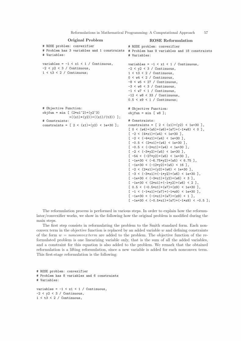
Reformulations in Mathematical Programming: A Computational Approach 57
Original Problem
# ROSE problem: convexifier
# Problem has 3 variables and 1 constraints
# Variables:
variables = -1 < x1 < 1 / Continuous,
-2 < y2 < 3 / Continuous,
1 < t3 < 2 / Continuous;
# Objective Function:
objfun = min [ (2*x1^2)+(y2^3)
+((x1)*(y2))+((x1)/(t3)) ];
ROSE Reformulation
# ROSE problem: convexifier
# Problem has 9 variables and 18 constraints
# Variables:
variables = -1 < x1 < 1 / Continuous,
-2 < y2 < 3 / Continuous,
1 < t3 < 2 / Continuous,
0 < w4 < 2 / Continuous,
-8 < w5 < 27 / Continuous,
-3 < w6 < 3 / Continuous,
-1 < w7 < 1 / Continuous,
-12 < w8 < 33 / Continuous,
0.5 < z9 < 1 / Continuous;
# Objective Function:
objfun = min [ w8 ];
# Constraints:
constraints = [ 2 < (x1)+(y2) < 1e+30 ];
# Constraints:
constraints = [ 2 < (x1)+(y2) < 1e+30 ],
[ 0 < (w4)+(w5)+(w6)+(w7)+(-1*w8) < 0 ],
[ -2 < (4*x1)+(w4) < 1e+30 ],
[ -2 < (-4*x1)+(w4) < 1e+30 ],
[ -0.5 < (2*x1)+(w4) < 1e+30 ],
[ -0.5 < (-2*x1)+(w4) < 1e+30 ],
[ -2 < (-3*y2)+(w5) < 1e+30 ],
[ -54 < (-27*y2)+(w5) < 1e+30 ],
[ -1e+30 < (-6.75*y2)+(w5) < 6.75 ],
[ -1e+30 < (-12*y2)+(w5) < 16 ],
[ -2 < (2*x1)+(y2)+(w6) < 1e+30 ],
[ -3 < (-3*x1)+(-1*y2)+(w6) < 1e+30 ],
[ -1e+30 < (-3*x1)+(y2)+(w6) < 3 ],
[ -1e+30 < (2*x1)+(-1*y2)+(w6) < 2 ],
[ 0.5 < (-0.5*x1)+(w7)+(z9) < 1e+30 ],
[ -1 < (-1*x1)+(w7)+(-1*z9) < 1e+30 ],
[ -1e+30 < (-1*x1)+(w7)+(z9) < 1 ],
[ -1e+30 < (-0.5*x1)+(w7)+(-1*z9) < -0.5 ];
The reformulation process is performed in various steps. In order to explain how the reformu-lator/convexifier works, we show in the following how the original problem is modified during themain steps.
The first step consists in reformulating the problem to the Smith standard form. Each non-convex term in the objective function is replaced by an added variable w and defining constraintsof the form w = nonconvex term are added to the problem. The objective function of the re-formulated problem is one linearizing variable only, that is the sum of all the added variables,and a constraint for this equation is also added to the problem. We remark that the obtainedreformulation is a lifting reformulation, since a new variable is added for each nonconvex term.This first-stage reformulation is the following:
# ROSE problem: convexifier
# Problem has 8 variables and 6 constraints
# Variables:
variables = -1 < x1 < 1 / Continuous,
-2 < y2 < 3 / Continuous,
1 < t3 < 2 / Continuous,

58 Leo Liberti, Sonia Cafieri, and Fabien Tarissan
0 < w4 < 2 / Continuous,
-8 < w5 < 27 / Continuous,
-3 < w6 < 3 / Continuous,
-1 < w7 < 1 / Continuous,
-12 < w8 < 33 / Continuous;
# Objective Function:
objfun = min [ w8 ];
# Constraints:
constraints = [ 2 < (x1)+(y2) < 1e+30 ],
[ 0 < (-1*w4)+(2*x1^2) < 0 ],
[ 0 < (-1*w5)+(y2^3) < 0 ],
[ 0 < (-1*w6)+((x1)*(y2)) < 0 ],
[ 0 < (-1*w7)+((x1)/(t3)) < 0 ],
[ 0 < (w4)+(w5)+(w6)+(w7)+(-1*w8) < 0 ];
Then, each defining constraint is replaced by a convex under-estimator and concave over-estimator of the corresponding nonlinear term. In particular, the term 2*x1^2 is treated as a convexunivariate function f(x) and a linear under-estimator is obtained by considering five tangents to f
at various given points, an over-estimator is obtained by considering the secant through the points(x1^L,f(x1^L)),(x1^U,f(x1^U)), where x1^L,and x1^U are the bounds on x1.For the termy2^3, where the range of y2 includes zero, the linear relaxation given in [80] is used. McCormick’senvelopes are considered for the bilinear term x1*y2.The fractional term is reformulated as bilinearby considering z=1/t3 and McCormick’s envelopes are exploited again. We obtain the followingrelaxation:
# ROSE problem: convexifier
# Problem has 9 variables and 22 constraints
# Variables:
variables = -1 < x1 < 1 / Continuous,
-2 < y2 < 3 / Continuous,
1 < t3 < 2 / Continuous,
0 < w4 < 2 / Continuous,
-8 < w5 < 27 / Continuous,
-3 < w6 < 3 / Continuous,
-1 < w7 < 1 / Continuous,
-12 < w8 < 33 / Continuous,
0.5 < z9 < 1 / Continuous;
# Objective Function:
objfun = min [ w8 ];
# Constraints:
constraints = [ 2 < (x1)+(y2) < 1e+30 ],
[ 0 < (-1*w4)+(2*x1^2) < 0 ],
[ 0 < (-1*w5)+(y2^3) < 0 ],
[ 0 < (-1*w6)+((x1)*(y2)) < 0 ],
[ 0 < (-1*w7)+((x1)/(t3)) < 0 ],
[ 0 < (w4)+(w5)+(w6)+(w7)+(-1*w8) < 0 ],
[ -2 < (4*x1)+(w4) < 1e+30 ],
[ -2 < (-4*x1)+(w4) < 1e+30 ],
[ -0.5 < (2*x1)+(w4) < 1e+30 ],
[ -0.5 < (-2*x1)+(w4) < 1e+30 ],
[ -2 < (-3*y2)+(w5) < 1e+30 ],

Reformulations in Mathematical Programming: A Computational Approach 59
[ -54 < (-27*y2)+(w55) < 1e+30 ],
[ -1e+30 < (-6.75*y2)+(w5) < 6.75 ],
[ -1e+30 < (-12*y2)+(w5) < 16 ],
[ -2 < (2*x1)+(y2)+(w6) < 1e+30 ],
[ -3 < (-3*x1)+(-1*y2)+(w6) < 1e+30 ],
[ -1e+30 < (-3*x1)+(y2)+(w6) < 3 ],
[ -1e+30 < (2*x1)+(-1*y2)+(w6) < 2 ],
[ 0.5 < (-0.5*x1)+(w7)+(z9) < 1e+30 ],
[ -1 < (-1*x1)+(w7)+(-1*z9) < 1e+30 ],
[ -1e+30 < (-1*x1)+(w7)+(z9) < 1 ],
[ -1e+30 < (-0.5*x1)+(w7)+(-1*z9) < -0.5 ];
Finally, the Smith defining constraints are removed, obtaining the final reformulation (of therelaxation type).
6 Conclusion
This chapter contains a study of mathematical programming reformulation and relaxation tech-niques. Section 1 presents some motivations towards such a study, the main being that MixedInteger Nonlinear Programming solvers need to be endowed with automatic reformulation capa-bilities before they can be as reliable, functional and efficient as their industrial-strength MixedInteger Linear Programming solvers are. Section 2 presents a general framework for represent-ing and manipulating mathematical programming formulations, as well as some definitions ofthe concept of reformulation together with some theoretical results; the section is concluded bylisting some of the most common standard forms in mathematical programming. In Section 3 wepresent a partial systematic study of existing reformulations. Each reformulation is presented bothin symbolic algorithmic terms (i.e. a prototype for carrying out the reformulation automaticallyin terms of the provided data structures is always supplied) and in the more usual mathematicalterms. This should be seen as the starting point for a more exhaustive study: eventually, all knownuseful reformulations might find their place in an automatic reformulation preprocessing softwarefor Mixed Integer Nonlinear Programming. In Section 4, we attempt a similar work with respectto relaxations. Section 5 describes the implementation of ROSE, a reformulation/optimizationsoftware engine.
Acknowledgements
Financial support by ANR grant 07-JCJC-0151 and by the EU NEST “Morphex” project grant isgratefully acknowledged. We also wish to thank: Claudia D’Ambrosio and David Savourey for helpon the ROSE implementation; Pierre Hansen, Nenad Mladenovic, Frank Plastria, Hanif Sheraliand Tapio Westerlund for many useful discussions and ideas; Kanika Dhyani and Fabrizio Marinellifor providing interesting application examples.
References
1. Adams, W., Forrester, R., Glover, F.: Comparisons and enhancement strategies for linearizing mixed0-1 quadratic programs. Discrete Optimization 1, 99–120 (2004)
2. Adams, W., Sherali, H.: A hierarchy of relaxations leading to the convex hull representation forgeneral discrete optimization problems. Annals of Operations Research 140, 21–47 (2005)
3. Adjiman, C., Dallwig, S., Floudas, C., Neumaier, A.: A global optimization method, αBB, for generaltwice-differentiable constrained NLPs: I. Theoretical advances. Computers & Chemical Engineering22(9), 1137–1158 (1998)

60 Leo Liberti, Sonia Cafieri, and Fabien Tarissan
4. Adjiman, C.S., Androulakis, I.P., Floudas, C.A.: A global optimization method, αBB, for generaltwice-differentiable constrained NLPs: II. Implementation and computational results. Computers &Chemical Engineering 22(9), 1159–1179 (1998)
5. Aho, A., Hopcroft, J., Ullman, J.: Data Structures and Algorithms. Addison-Wesley, Reading, MA(1983)
6. Al-Khayyal, F., Falk, J.: Jointly constrained biconvex programming. Mathematics of OperationsResearch 8(2), 273–286 (1983)
7. Alizadeh, F.: Interior point methods in semidefinite programming with applications to combinatorialoptimization. SIAM Journal on Optimization 5(1), 13–51 (1995)
8. Andersen, K., Cornuejols, G., Li, Y.: Reduce-and-split cuts: Improving the performance of mixed-integer gomory cuts. Management Science 51(11), 1720–1732 (2005)
9. Androulakis, I.P., Maranas, C.D., Floudas, C.A.: αBB: A global optimization method for generalconstrained nonconvex problems. Journal of Global Optimization 7(4), 337–363 (1995)
10. Anstreicher, K.: SDP versus RLT for nonconvex QCQPs. In: C. Floudas, P. Pardalos (eds.) Proceed-ings of Advances in Global Optimization: Methods and Applications. Mykonos, Greece (2007)
11. Applegate, D., Bixby, R., Chvatal, V., Cook, W.: The Travelling Salesman Problem: a ComputationalStudy. Princeton University Press, Princeton (2007)
12. Audet, C., Hansen, P., Jaumard, B., Savard, G.: Links between linear bilevel and mixed 0-1 pro-gramming problems. Journal of Optimization Theory and Applications 93(2), 273–300 (1997)
13. Balas, E.: Intersection cuts — A new type of cutting planes for integer programming. OperationsResearch 19(1), 19–39 (1971)
14. Balas, E.: Projection, lifting and extended formulation in integer and combinatorial optimization.Annals of Operations Research 140, 125–161 (2005)
15. Balas, E., Jeroslow, R.: Canonical cuts on the unit hypercube. SIAM Journal on Applied Mathematics23(1), 61–69 (1972)
16. Bauer, C., Frink, A., Kreckel, R.: Introduction to the GINaC framework for symbolic computationwithin the C++ programming language. Journal of Symbolic Computation 33(1), 1–12 (2002)
17. Belotti, P., Lee, J., Liberti, L., Margot, F., Wachter, A.: Branching and bounds tightening techniquesfor non-convex MINLPs. Optimization Methods and Software (submitted)
18. Bjork, K.M., Lindberg, P., Westerlund, T.: Some convexifications in global optimization of problemscontaining signomial terms. Computers & Chemical Engineering 27, 669–679 (2003)
19. Bjorkqvist, J., Westerlund, T.: Automated reformulation of disjunctive constraints in MINLP opti-mization. Computers & Chemical Engineering 23, S11–S14 (1999)
20. Boyd, E.: Fenchel cutting planes for integer programs. Operations Research 42(1), 53–64 (1994)21. Boyd, S., Vandenberghe, L.: Convex Optimization. Cambridge University Press, Cambridge (2004)22. Brook, A., Kendrick, D., Meeraus, A.: GAMS, A user’s guide. ACM SIGNUM Newsletter 23(3-4),
10–11 (1988)23. Caporossi, G., Alamargot, D., Chesnet, D.: Using the computer to study the dyamics of the hand-
writing processes. In: DS 2004 Proceedings, LNAI, vol. 3245, pp. 242–254. Springer-Verlag (2004)24. Cornuejols, G.: Valid inequalities for mixed integer linear programs. Mathematical Programming B
112(1), 3–44 (2008)25. Cortellessa, V., Marinelli, F., Potena, P.: Automated selection of software components based on
cost/reliability tradeoff. In: V. Gruhn, F. Oquendo (eds.) EWSA 2006, LNCS, vol. 4344, pp. 66–81.Springer-Verlag (2006)
26. Dantzig, G.: Linear Programming and Extensions. Princeton University Press, Princeton, NJ (1963)27. Davidovic, T., Liberti, L., Maculan, N., Mladenovic, N.: Towards the optimal solution of the multi-
processor scheduling problem with communication delays. In: MISTA Proceedings (2007)28. Dhyani, K.: Personal communication (2007)29. Di Giacomo, L.: Mathematical programming methods in dynamical nonlinear stochastic supply chain
management. Ph.D. thesis, DSPSA, Universita di Roma “La Sapienza” (2007)30. Duran, M., Grossmann, I.: An outer-approximation algorithm for a class of mixed-integer nonlinear
programs. Mathematical Programming 36, 307–339 (1986)31. Falk, J., Liu, J.: On bilevel programming, part I: General nonlinear cases. Mathematical Programming
70, 47–72 (1995)32. Falk, J., Soland, R.: An algorithm for separable nonconvex programming problems. Management
Science 15, 550–569 (1969)33. Fischer, A.: New constrained optimization reformulation of complementarity problems. Journal of
Optimization Theory and Applications 99(2), 481–507 (1998)

Reformulations in Mathematical Programming: A Computational Approach 61
34. Fletcher, R., Leyffer, S.: Solving mixed integer nonlinear programs by outer approximation. Mathe-matical Programming 66, 327–349 (1994)
35. Floudas, C.: Deterministic Global Optimization. Kluwer Academic Publishers, Dordrecht (2000)36. Fortet, R.: Applications de l’algebre de boole en recherche operationelle. Revue Francaise de
Recherche Operationelle 4, 17–26 (1960)37. Fourer, R.: Personal communication (2004)38. Fourer, R., Gay, D.: The AMPL Book. Duxbury Press, Pacific Grove (2002)39. Galli, S.: Parsing AMPL internal format for linear and non-linear expressions (2004). B.Sc. Disser-
tation, DEI, Politecnico di Milano, Italy40. Gill, P.: User’s Guide for SNOPT 5.3. Systems Optimization Laboratory, Department of EESOR,
Stanford University, California (1999)41. Gill, P.: User’s guide for SNOPT version 7. Systems Optimization Laboratory, Stanford University,
California (2006)42. Gomory, R.: Essentials of an algorithm for integer solutions to linear programs. Bulletin of the
American Mathematical Society 64(5), 256 (1958)43. Grant, M., Boyd, S., Ye, Y.: Disciplined convex programming. In: Liberti and Maculan [79], pp.
155–21044. Gueret, C., Prins, C., Sevaux, M.: Applications of optimization with Xpress-MP. Dash Optimization,
Bilsworth (2000)45. Hammer, P., Rudeanu, S.: Boolean Methods in Operations Research and Related Areas. Springer,
Berlin (1968)46. Hansen, P.: Method of non-linear 0-1 programming. Annals of Discrete Mathematics 5, 53–70 (1979)47. Haverly, C.: Studies of the behaviour of recursion for the pooling problem. ACM SIGMAP Bulletin
25, 19–28 (1978)48. Horst, R.: On the convexification of nonlinear programming problems: an applications-oriented ap-
proach. European Journal of Operations Research 15, 382–392 (1984)49. Horst, R., Tuy, H.: Global Optimization: Deterministic Approaches, 3rd edition. Springer-Verlag,
Berlin (1996)50. Horst, R., Van Thoai, N.: Duality bound methods in global optimization. In: C. Audet, P. Hansen,
G. Savard (eds.) Essays and Surveys in Global Optimization, pp. 79–105. Springer, Berlin (2005)51. ILOG: ILOG CPLEX 8.0 User’s Manual. ILOG S.A., Gentilly, France (2002)52. ILOG: ILOG CPLEX 11.0 User’s Manual. ILOG S.A., Gentilly, France (2008)53. Judice, J., Mitra, G.: Reformulation of mathematical programming problems as linear complemen-
tarity problems and investigation of their solution methods. Journal of Optimization Theory andApplications 57(1), 123–149 (1988)
54. Kaibel, V., Pfetsch, M.: Packing and partitioning orbitopes. Mathematical Programming 114(1),1–36 (2008)
55. Kaltofen, E.: Challenges of symbolic computation: My favorite open problems. Journal of SymbolicComputation 29, 891–919 (2000). URL citeseer.nj.nec.com/article/kaltofen99challenge.
html
56. Kelley, J.: The cutting plane method for solving convex programs. Journal of SIAM VIII(6), 703–712(1960)
57. Kesavan, P., Allgor, R., Gatzke, E., Barton, P.: Outer-approximation algorithms for nonconvexmixed-integer nonlinear programs. Mathematical Programming 100(3), 517–535 (2004)
58. Kojima, M., Megiddo, N., Ye, Y.: An interior point potential reduction algorithm for the linearcomplementarity problem. Mathematical Programming 54, 267–279 (1992)
59. Konno, H.: A cutting plane algorithm for solving bilinear programs. Mathematical Programming11, 14–27 (1976)
60. Kucherenko, S., Belotti, P., Liberti, L., Maculan, N.: New formulations for the kissing number prob-lem. Discrete Applied Mathematics 155(14), 1837–1841 (2007)
61. Kucherenko, S., Sytsko, Y.: Application of deterministic low-discrepancy sequences in global opti-mization. Computational Optimization and Applications 30(3), 297–318 (2004)
62. Kunen, K.: Set Theory. An Introduction to Independence Proofs. North Holland, Amsterdam (1980)63. Lavor, C., Liberti, L., Maculan, N.: Computational experience with the molecular distance geometry
problem. In: J. Pinter (ed.) Global Optimization: Scientific and Engineering Case Studies, pp. 213–225. Springer, Berlin (2006)
64. Lavor, C., Liberti, L., Maculan, N., Chaer Nascimento, M.: Solving Hartree-Fock systems with globaloptimization metohds. Europhysics Letters 5(77), 50,006p1–50,006p5 (2007)

62 Leo Liberti, Sonia Cafieri, and Fabien Tarissan
65. Letchford, A., Lodi, A.: Strengthening Chvatal-Gomory cuts and Gomory fractional cuts. OperationsResearch Letters 30, 74–82 (2002)
66. Liberti, L.: Framework for symbolic computation in C++ using n-ary trees. Tech. rep., CPSE,Imperial College London (2001)
67. Liberti, L.: Comparison of convex relaxations for monomials of odd degree. In: I. Tseveendorj,P. Pardalos, R. Enkhbat (eds.) Optimization and Optimal Control. World Scientific (2003)
68. Liberti, L.: Reduction constraints for the global optimization of NLPs. International Transactionsin Operational Research 11(1), 34–41 (2004)
69. Liberti, L.: Reformulation and convex relaxation techniques for global optimization. 4OR 2, 255–258(2004)
70. Liberti, L.: Reformulation and convex relaxation techniques for global optimization. Ph.D. thesis,Imperial College London, UK (2004)
71. Liberti, L.: Linearity embedded in nonconvex programs. Journal of Global Optimization 33(2),157–196 (2005)
72. Liberti, L.: Writing global optimization software. In: Liberti and Maculan [79], pp. 211–26273. Liberti, L.: Compact linearization of binary quadratic problems. 4OR 5(3), 231–245 (2007)74. Liberti, L.: Reformulations in mathematical programming: Definitions. In: R. Aringhieri, R. Cordone,
G. Righini (eds.) Proceedings of the 7th Cologne-Twente Workshop on Graphs and CombinatorialOptimization, pp. 66–70. Universita Statale di Milano, Crema (2008)
75. Liberti, L.: Spherical cuts for integer programming problems. International Transactions in Opera-tional Research 15, 283–294 (2008)
76. Liberti, L., Drazic, M.: Variable neighbourhood search for the global optimization of constrainedNLPs. In: Proceedings of GO Workshop, Almeria, Spain (2005)
77. Liberti, L., Lavor, C., Maculan, N.: Double VNS for the molecular distance geometry problem. In:Proc. of Mini Euro Conference on Variable Neighbourhood Search, Tenerife, Spain (2005)
78. Liberti, L., Lavor, C., Nascimento, M.C., Maculan, N.: Reformulation in mathematical programming:an application to quantum chemistry. Discrete Applied Mathematics (accepted for publication)
79. Liberti, L., Maculan, N. (eds.): Global Optimization: from Theory to Implementation. Springer,Berlin (2006)
80. Liberti, L., Pantelides, C.: Convex envelopes of monomials of odd degree. Journal of Global Opti-mization 25, 157–168 (2003)
81. Liberti, L., Pantelides, C.: An exact reformulation algorithm for large nonconvex NLPs involvingbilinear terms. Journal of Global Optimization 36, 161–189 (2006)
82. Liberti, L., Tsiakis, P., Keeping, B., Pantelides, C.: ooOPS. Centre for Process Systems Engineering,Chemical Engineering Department, Imperial College, London, UK (2001)
83. Lougee-Heimer, R.: The common optimization interface for operations research: Promoting open-source software in the operations research community. IBM Journal of Research and Development47(1), 57–66 (2003)
84. Maculan, N., Macambira, E., de Souza, C.: Geometrical cuts for 0-1 integer programming. Tech.Rep. IC-02-006, Instituto de Computacao, Universidade Estadual de Campinas (2002)
85. Makhorin, A.: GNU Linear Programming Kit. Free Software Foundation,http://www.gnu.org/software/glpk/ (2003)
86. Mangasarian, O.: Linear complementarity problems solvable by a single linear program. Mathemat-ical Programming 10, 263–270 (1976)
87. Mangasarian, O.: The linear complementarity problem as a separable bilinear program. Journal ofGlobal Optimization 6, 153–161 (1995)
88. Maranas, C.D., Floudas, C.A.: Finding all solutions to nonlinearly constrained systems of equations.Journal of Global Optimization 7(2), 143–182 (1995)
89. Margot, F.: Pruning by isomorphism in branch-and-cut. Mathematical Programming 94, 71–90(2002)
90. Margot, F.: Exploiting orbits in symmetric ILP. Mathematical Programming B 98, 3–21 (2003)91. McCormick, G.: Computability of global solutions to factorable nonconvex programs: Part I —
Convex underestimating problems. Mathematical Programming 10, 146–175 (1976)92. Meyer, C., Floudas, C.: Trilinear monomials with mixed sign domains: Facets of the convex and
concave envelopes. Journal of Global Optimization 29, 125–155 (2004)93. Mladenovic, N., Plastria, F., Urosevic, D.: Reformulation descent applied to circle packing problems.
Computers and Operations Research 32(9), 2419–2434 (2005)94. Nemhauser, G., Wolsey, L.: Integer and Combinatorial Optimization. Wiley, New York (1988)

Reformulations in Mathematical Programming: A Computational Approach 63
95. Nowak, I.: Relaxation and Decomposition Methods for Mixed Integer Nonlinear Programming.Birkhauser, Basel (2005)
96. Pantelides, C., Liberti, L., Tsiakis, P., Crombie, T.: Mixed integer linear/nonlinear programminginterface specification. Global Cape-Open Deliverable WP2.3-04 (2002)
97. Pardalos, P., Romeijn, H. (eds.): Handbook of Global Optimization, vol. 2. Kluwer Academic Pub-lishers, Dordrecht (2002)
98. Plateau, M.C.: Reformulations quadratiques convexes pour la programmation quadratique en vari-ables 0-1. Ph.D. thesis, Conservatoire National d’Arts et Metiers (2006)
99. Puchinger, J., Raidl, G.: Relaxation guided variable neighbourhood search. In: Proc. of Mini EuroConference on Variable Neighbourhood Search, Tenerife, Spain (2005)
100. Raghavachari, M.: On connections between zero-one integer programming and concave programmingunder linear constraints. Operations Research 17(4), 680–684 (1969)
101. van Roy, T., Wolsey, L.: Solving mixed integer programming problems using automatic reformulation.Operations Research 35(1), 45–57 (1987)
102. Ryoo, H., Sahinidis, N.: Global optimization of nonconvex NLPs and MINLPs with applications inprocess design. Computers & Chemical Engineering 19(5), 551–566 (1995)
103. Sherali, H.: Global optimization of nonconvex polynomial programming problems having rationalexponents. Journal of Global Optimization 12, 267–283 (1998)
104. Sherali, H.: Tight relaxations for nonconvex optimization problems using the reformulation-linearization/convexification technique (RLT). In: Pardalos and Romeijn [97], pp. 1–63
105. Sherali, H.: Personal communication (2007)106. Adams, W., Sherali, H.: A tight linearization and an algorithm for 0-1 quadratic programming
problems. Management Science 32(10), 1274–1290 (1986)107. Sherali, H., Adams, W.: A hierarchy of relaxations between the continuous and convex hull repre-
sentations for zero-one programming problems. SIAM Journal of Discrete Mathematics 3, 411–430(1990)
108. Sherali, H., Adams, W.: A Reformulation-Linearization Technique for Solving Discrete and Contin-uous Nonconvex Problems. Kluwer Academic Publishers, Dodrecht (1999)
109. Sherali, H., Alameddine, A.: A new reformulation-linearization technique for bilinear programmingproblems. Journal of Global Optimization 2, 379–410 (1992)
110. Sherali, H., Liberti, L.: Reformulation-linearization methods for global optimization. In: C. Floudas,P. Pardalos (eds.) Encyclopedia of Optimization. Springer, New York (to appear)
111. Sherali, H., Tuncbilek, C.: New reformulation linearization/convexification relaxations for univariateand multivariate polynomial programming problems. Operations Research Letters 21, 1–9 (1997)
112. Sherali, H., Wang, H.: Global optimization of nonconvex factorable programming problems. Mathe-matical Programming 89, 459–478 (2001)
113. Smith, E.: On the optimal design of continuous processes. Ph.D. thesis, Imperial College of Science,Technology and Medicine, University of London (1996)
114. Smith, E., Pantelides, C.: Global optimisation of nonconvex MINLPs. Computers & Chemical En-gineering 21, S791–S796 (1997)
115. Smith, E., Pantelides, C.: A symbolic reformulation/spatial branch-and-bound algorithm for theglobal optimisation of nonconvex MINLPs. Computers & Chemical Engineering 23, 457–478 (1999)
116. Strekalovsky, A.: On global optimality conditions for d.c. programming problems. Technical Paper,Irkutsk State University (1997)
117. Strekalovsky, A.: Extremal problems with d.c. constraints. Computational Mathematics and Math-ematical Physics 41(12), 1742–1751 (2001)
118. Stroustrup, B.: The C++ Programming Language, 3rd edition. Addison-Wesley, Reading, MA (1999)119. Sutou, A., Dai, Y.: Global optimization approach to unequal sphere packing problems in 3D. Journal
of Optimization Theory and Applications 114(3), 671–694 (2002)120. Tardella, F.: Existence and sum decomposition of vertex polyhedral convex envelopes. Optimization
Letters 2, 363–375 (2008)121. Tawarmalani, M., Ahmed, S., Sahinidis, N.: Global optimization of 0-1 hyperbolic programs. Journal
of Global Optimization 24, 385–416 (2002)122. Tawarmalani, M., Sahinidis, N.: Semidefinite relaxations of fractional programming via novel tech-
niques for constructing convex envelopes of nonlinear functions. Journal of Global Optimization20(2), 137–158 (2001)
123. Tawarmalani, M., Sahinidis, N.: Convex extensions and envelopes of semi-continuous functions. Math-ematical Programming 93(2), 247–263 (2002)

64 Leo Liberti, Sonia Cafieri, and Fabien Tarissan
124. Tawarmalani, M., Sahinidis, N.: Exact algorithms for global optimization of mixed-integer nonlinearprograms. In: Pardalos and Romeijn [97], pp. 65–86
125. Tawarmalani, M., Sahinidis, N.: Global optimization of mixed integer nonlinear programs: A theo-retical and computational study. Mathematical Programming 99, 563–591 (2004)
126. Todd, M.: Semidefinite optimization. Acta Numerica 10, 515–560 (2001)127. Tsiakis, P., Keeping, B.: ooMILP — A C++ callable object-oriented library and the implementation
of its parallel version using CORBA. In: Liberti and Maculan [79], pp. 155–210128. Tsiakis, P., Keeping, B., Pantelides, C.: ooMILP. Centre for Process Systems Engineering, Chemical
Engineering Department, Imperial College, London, UK, 0.7 edn. (2000)129. Tuy, H.: Concave programming under linear constraints. Soviet Mathematics pp. 1437–1440 (1964)130. Tuy, H.: D.c. optimization: Theory, methods and algorithms. In: R. Horst, P. Pardalos (eds.) Hand-
book of Global Optimization, vol. 1, pp. 149–216. Kluwer Academic Publishers, Dordrecht (1995)131. Wang, X., Change, T.: A multivariate global optimization using linear bounding functions. Journal
of Global Optimization 12, 383–404 (1998)132. Westerlund, T.: Some transformation techniques in global optimization. In: Liberti and Maculan
[79], pp. 45–74133. Westerlund, T., Skrifvars, H., Harjunkoski, I., Porn, R.: An extended cutting plane method for a
class of non-convex MINLP problems. Computers & Chemical Engineering 22(3), 357–365 (1998)134. Wolsey, L.: Integer Programming. Wiley, New York (1998)135. Zamora, J.M., Grossmann, I.E.: A branch and contract algorithm for problems with concave univari-
ate, bilinear and linear fractional terms. Journal of Global Optimization 14, 217:249 (1999)
Index
α-underestimator, 31αBB algorithm, 31
AbsDiff, 18, 22absolute value
minimization, 22affine, 35algorithm, 1
efficient, 30generic, 1heuristic, 30NLP, 2symbolic, 2
alphabet, 5AMPL, 3AND, 21approximation, 30
outer, 30polyhedral, 30
architecture, 26assignment, 24
constraint, 19variable, 19variables, 24
BARON, 32BB, 12bijection, 14bilevel problem, 12bilevel programming, 12bilinear, 15Bin2Cont, 18binary
product, 20representation, 18
BinaryRep, 19BIP, 38bisection, 2blending problem, 34block-separable, 33BLP, 12bound, 29, 30
lower, 33
bound factor, 31, 34boundary point, 30bounds, 5branch-and-bound, 3, 9, 12, 29, 32, 37
pruning, 15spatial, 32, 35
branch-and-contract, 32
cardinality, 1CAS, 3CCLin, 22clustering, 6, 24complementarity
constraints, 21complexity theory, 14complicating constraints, 33ConSense, 16constants, 18constraint, 4, 5
assignment, 24, 27binary, 18complicating, 33defining, 32, 35, 36equality, 17inequality, 17nonconvex, 18nonlinear, 18ordering, 3, 18quadratic, 12, 18qualification, 33relaxation, 35, 37reliability, 27sense, 16soft, 2valid, 34
constraint factor, 34constraint relaxation, 19constraint tolerance, 19convex
envelope, 15function, 15hull, 15
convex envelope, 31, 34, 35

66 Index
coordinatesEuclidean, 3spherical, 3
cost, 26CPLEX, 3, 26cut
deeper, 39Gomory, 38intersection, 38interval-gradient, 39knapsack, 39Lagrangian, 39level, 39linearization, 39NLP, 39spherical, 38valid, 38
cuts, 15MIR, 38Reduce-and-split, 38
cutset, 13cutting plane, 37
convergence, 38
d.c.function, 11problem, 11set, 11
DAG, 5, 8data structure, 33decidable, 1decision problem, 14decomposition, 2dense, 11differentiable, 25distance
minimum, 24distance geometry, 34distribute
products over sums, 29domain
partition, 29duality
Fenchel, 38duality gap, 12
efficiency, 1eigenvalue
minimum, 31enumeration
complete, 1implicit, 29
envelopeconvex, 32polyhedral, 32
equationunivariate, 18
evaluation, 8exponent, 9, 19
exponential, 36expression, 4, 5
nonlinear, 18standard form, 9tree, 5, 8
expression tree, 4
factorbound, 34constraint, 34
factorable, 11Feas2Opt, 19feasible, 13
bounds, 13constraints, 13point, 11, 13region, 37type, 13
feasible regionconvex, 30
FixQB, 23follower, 12form
factorable, 11separable, 10standard, 9, 30
formulation, 1, 8, 9mathematical programming, 4
fractional, 15function
continuous, 33exponential, 36power, 36pseudoconvex, 38signomial, 36transformation, 36univariate, 31
Godel, 1GAMS, 32global
optimality condition, 11optimum, 15
GO, 18Gomory cuts, 38graph
bisection, 6directed acyclic, 5partitioning, 6
graph bisection, 34graph partitioning, 34group
cuts, 38
half-line, 38HCP, 24Hessian, 31heuristic, 30hypercube
Index 67
unit, 38hyperplane, 24, 38Hyperplane Clustering Problem, 24hypersphere, 38
identity, 17, 19ILOG, 26incumbent, 29inequality
linear, 37polynomial, 35
infeasible, 13input, 1Int2Bin, 19interior point method, 12intersection cuts, 38IP, 38IPM, 12iteration, 37
kissing number, 2, 7Kissing Number Problem, 2, 34KNP, 2, 8, 34
Lagrangian decomposition, 33Lagrangian problem, 33Lagrangian relaxation, 33language, 14LCP, 11leader, 12leaf, 8leaf node, 19Lift, 16lift-and-project, 34, 38lifting, 2, 13, 16, 17, 35linear
equation, 1form, 1, 9mixed integer, 9programming, 9
linear complementarity, 11linear fractional, 22linear programming, 1linearization, 20LinFract, 22logarithm, 18, 28LP, 1, 9, 17, 30, 33
standard form, 9
mathematical programming, 14, 19matrix, 4, 8
symmetric, 34McCormick envelopes, 31MDGP, 34MILP, 3, 9, 12, 24, 26, 29, 30, 37
solver, 26standard form, 9
MinAbs, 22minimality
local, 20MINLP, 10, 24, 27, 29, 30, 32, 33
convex, 37quadratic, 33solver, 26standard form, 39
MinMax, 20MIR cuts, 38molecular distance geometry, 34monomial, 36
multivariate, 36odd degree, 15
monotonically increasing, 28multiplier, 8
NLP, 2, 10, 18, 30, 33convex, 12nonconvex, 29standard form, 10
nonconvex, 2, 12, 30, 34nonlinear
mixed integer, 10programming, 10
NP-completeness, 14NP-hard, 12
OA, 30ObjDir, 16objective
linear, 38quadratic, 12
objective function, 4, 5, 14operator, 5, 8
argument, 8max, 33power, 9product, 9sum, 9
opt-reformulation, 15, 19, 36optimality, 33
condition, 11global, 13guarantee, 26local, 14
optimizationdirection, 5, 16global, 18
optimization problem, 14optimum
global, 13, 14, 19, 25local, 13, 19
outer approximation, 30, 32output, 1overestimator
concave, 32
parameter, 4, 5partition
balanced, 13

68 Index
piecewiselinear, 20
point, 13polynomial, 9polynomial time, 14pooling problem, 34potential transformation, 36power, 9, 36problem
auxiliary, 2, 15, 35bilevel, 12binary, 18blending, 32, 34decision, 1, 2, 14, 19distance geometry, 32feasibility, 2, 19follower, 12graph partitioning, 34kissing number, 7Lagrangian, 33leader, 12molecular distance geometry, 34multilevel, 4, 8optimization, 1, 14, 19polynomial, 36pooling, 32, 34pseudoconvex, 38quadratic, 18quantum chemistry, 32reformulated, 36scheduling, 34SDP, 12semidefinite, 4, 12signomial, 36structure, 9, 38
ProdBin, 20ProdBinCont, 21, 56ProdExp, 18product, 9
binary, 29binary and continuous, 21, 56binary variables, 20exponential, 18quadratic, 35
programmingmathematical, 1mixed-integer linear, 3nonlinear, 2
Proj, 17projection, 2, 16, 17, 19, 36pseudoconvex, 38
function, 38problem, 38
QCQP, 12, 33quadratic, 12quadratically constrained, 12
MINLP, 33
range reduction, 32recursion, 29RedCon, 24Reduce-and-split cuts, 38redundant inequality, 37reformulation, 4, 14
automatic, 29cardinality, 29definition, 13global, 15, 33local, 14MILP, 24product, 29step, 34symbolic, 32
relaxation, 2, 29bound, 30constraint, 30, 35continuous, 30, 33convex, 30, 32, 33, 57elementary, 30hierarchy, 35, 38Lagrangian, 32, 33linear, 3LP, 32McCormick, 35RLT, 32scheme, 30semidefinite, 32signomial, 32tightness, 33
reliability, 26Restrict, 16, 23restriction, 16reverse convex, 2RLT, 34, 35
hierarchy, 36second-level, 31
robustnessnumerical, 26
sBB, 30, 32, 35scalability, 26scheduling
communication delays, 34SDP, 12, 33
dual, 12primal, 12
semantic interpretation, 29separable, 10sequential quadratic programming, 10signomial, 36signomial function, 36simplex
tableau, 38simplex method, 9, 10, 17Slack, 17SNOPT, 2software

Index 69
architecture, 26component, 26system, 26
solutionbasic, 38feasible, 18optimal feasible, 9starting, 2symmetry, 15time, 37
solver, 26NLP, 2
sphere, 2spherical cuts, 38SQP, 10stability
numerical, 26standard form, 9
expression, 9LP, 9MILP, 9MINLP, 39NLP, 10Smith, 32, 35, 36
subdomain, 29sum, 9symmetry, 3
breaking, 18group, 15
systemsoftware, 26
tangent, 30term
bilinear, 31, 32, 35fractional, 31, 32linear fractional, 22monomial, 36
nonconvex, 31, 33nonlinear, 18piecewise convex/concave, 32quadratic, 29, 34signomial, 36trilinear, 31univariate, 32univariate concave, 31
transformationpotential, 36
treeBB, 12
trilinear, 15twice-differentiable, 31
underestimatorconvex, 32secant, 31
uniform convergence, 11
valid cut, 37MILP, 38
valid inequality, 37linear, 37
variable, 4, 5added, 35, 36assignment, 18, 28binary, 5, 18bounds, 5continuous, 5, 9, 30discrete, 30domain, 29general integer, 18integer, 5, 28, 30linearization, 29transformation, 14
Zermelo-Frankel, 1ZFC, 1