Working Paper Series

Reformulating Technical Change and Growth TheoryGary Jefferson Economics Department, Brandeis University

2017| 111

1

`

Reformulating Technical Change and Growth Theory*

Gary H. Jefferson jefferson@brandeis.edu

Brandeis University

February 28, 2017

For review and comment only Suggestions will be most welcome

Abstract

This paper clarifies certain errors and inconsistencies that have become embedded in the conventional neoclassical growth model. The paper demonstrates that characterizing technical change in the Solow model as “purely Harrod-neutral labor augmenting” seriously compromises the role of capital and neoclassical principles in framing the process of economic growth. The basic argument of this paper is that by ignoring the actual elements of the so-called “degeneration” of Hicks-neutral or other capital-labor augmenting technical change, conventional presentations of the Solow model have foreclosed avenues for a deeper understanding of key features of economic growth. The paper develops the paradigm of Hick-Harrod technical change that is consistent with steady state growth under a wide range of values of the substitution elasticity, while also enabling a simplification of conditions required for the steady state. By endogenizing significant aspects of the growth process, the model opens the door to possibilities for a more unified theory of neoclassical growth, endogenous growth, and growth accounting.

*The author deeply appreciates the opportunity to have presented portions of this paper in seminars in the Economics Department at Brandeis and at the Department of Economics at the University of Macau. In particular, the author appreciates the helpful suggestions and support of George Hall, as well as suggestions from Michael Coiner, Adam Jaffe, Fung Kwan, James Mirrlees, Dwight Perkins, Tom Rawski, Jian Su, and Tony Yezer. The author alone is responsible for the content of this paper.

2

“There are always aspects of economic life that are left out of any simplified model. There will therefore be problems on which it throws no light at all; worse yet, there

may be problems on which it appears to throw light, but on which it actually propagates error.”

Robert M. Solow (2000, pp. 1,2)

“If I have seen further it is by standing on the shoulders of giants.”

Sir Issac Newton (1676)

3

1. Introduction

The economics literature is amply sprinkled with congratulatory assessments of the

achievements of growth theory. According to Aghion and Howitt (2007, p. 79):

Fifty years after its publication, the Solow model remains the unavoidable benchmark in growth economics, the equivalent of what the Modigliani–Miller theorem is to corporate finance, or the Arrow–Debreu model is to microeconomics….

In Chapter 8 of his tome, Introduction to Modern Economic Growth Theory, Acemoglu (2009)

variously refers to the Solow model as “the workhorse model of macroeconomics” (p. 26) and

“the most important model in macroeconomics” (p. 317). Finally, in their paper, Jones and

Romer (2010, p. 225) assert a conclusive consensus framing the canonical growth model: “There

is no longer any interesting debate about the features that a model must contain to explain [the

Kaldor facts]. These features are embedded in one of the great successes of growth theory in the

1950s and 1960s, the neoclassical growth model.”

Specifically, the model seeks to capture within a single economic framework the

following six stylized facts of growth summarized by Kaldor (1961): output per capita grows

over time; the capital-labor ratio grows over time; capital’s marginal product is roughly constant

over time; the capital output ratio is roughly constant over time; capital and labor’s factor income

shares are roughly constant over time; and the growth of output per capita differs substantially

across countries.

While Solow’s model (1956) explains or is consistent with five of these six stylized facts,

it does an inadequate job of modeling and explaining the last of the facts; that is the difference in

the growth of living standards across countries. As such, it is also largely unable to explain

differences in cross-country levels of output per capita (Romer, 1994b). The inability of the

neoclassical growth model to embed a parameter or equation to explain these differences has

given rise to an abundance of endogenous growth literature, which while rich and diverse has not

yet resulted in a single, widely-accepted account of the creation and diffusion of technical change

comparable to the consensus enjoyed by Solow’s seminal innovation.

In addition, Kaldor’s list of stylized growth facts omits one critical fact of long-run

growth: that is, the phenomenon in which the quality of capital progresses over time. That this

4

measure of technical advance should not be included in an economist’s list of stylized facts is not

altogether surprising, since the sine qua non of the economist’s measure of quality improvement

is the factor’s marginal product. Kaldor correctly notes that over the long-run, capital’s marginal

product and its economic return have remained roughly constant. Yet, through the lens of casual

observation, capital’s constant economic return does not negate the fact that the machinery and

processes driving manufacturing activity, as well as its production outcomes, such as communi-

cation and transportation equipment, including air and space travel, are far more accessible,

efficient, and inexpensive than they had been in the Stone Age. It is precisely this progressive

improvement in the quality of capital, the essence of the Industrial Revolution that has been most

responsible for capital deepening and rising living standards. This critical stylized fact of

economic growth – quality improvements in capital – is entirely absent from Solow’s model.

The ability of the basic neoclassical model to incorporate quality-augmenting technical

change for capital has been seriously impaired by a central principle of steady state growth; that

is the requirement that in the steady state technical change must take the form of “purely labor –

augmenting” Harrod-neutral technical change. This characterization of technical change has its

origins in Uzawa’s Growth Theorem (1961) in which he shows that if in the steady state the

capital-output ratio is fixed and if output and capital together grow faster than the natural growth

of labor, then the “effective” supply of labor must be balanced by labor-augmenting technical

change. Hence, technical change in the steady state must be “represented” as being of the purely

labor-augmenting variety. As elaborated by Jones and Scrimgeour (2005, p. 4), “As is well-

known, in the case of Cobb-Douglas production, capital- and labor-augmenting technical change

are equivalent. One sometimes sees the theorem interpreted as saying that technical change must

be labor augmenting or the production function must be Cobb-Douglas. This is equivalent

to the statement of the (Uzawa) theorem as given.” i.e., that in the steady state technical change

must be represented as labor augmenting (italics added).

Thus, given that with the Cobb-Douglas function, all the alternative forms of technical

change degenerate in the steady state to the labor-augmenting mode and that the Cobb-Douglas

function is limited to the restrictive case of a unitary substitution elasticity (i.e., σ = 1), the

literature has rendered “purely labor-augmenting” Harrod-neutral technical change as a canonical

feature of the neoclassical growth model. Hence, within the environment of a Cobb-Douglas

production function with σ = 1, the growth literature seems to have adopted the presumption of

5

technical change equivalency. Many attempt clarifying explanations for this restrictive

interpretation of technical change. Grossman et al. (2016) explain: “The ‘problem,’ it would

seem, stems from the model’s assumption of an inelastic supply of effective labor that does not

adjust to capital deepening over time.” Jones and Scrimgeour (2005) are more explicit about the

passive role of the capital stock whose function it is to “inherit” or endogenously submit to the

conditions presented to it by exogenous change, which is purely labor-centric.

Hence the “workhorse” of neoclassical growth theory and the “workhorse” of production

technology, the Cobb-Douglas production function, share an uneasy relationship that has resulted

in a deeply unsettling outcome: the basic model of neoclassical growth cannot account for or

accommodate to a fundamental and inescapable stylized fact of long-run economic growth – that

is, quality improvements in the ever-expanding realm of capital goods. Given this dependence of

our basic textbooks account of economic growth as “purely labor augmenting,” it is

understandable why both Solow and Acemoglu have raised serious reservations regarding the

assumption of the nature of technical change in long-run growth. According to Solow (2000, p.

31,32), “…it is possible to give theoretical reasons why technological progress might be forced

to assume the particular form (“called labor-augmenting”) required for the existence of a steady

state. They are excessively fancy reasons, not altogether believable.” Acemogulu (2009, pp. 62)

simply characterizes the assumption as “At some level…distressing.”

Arguably the Solow model co-exists with both a weak-form of the Uzawa Theorem and a

strong form. According to the weak form, within the “neighborhood of the equilibrium path,”

technical change must be represented as labor-augmenting Harrod-neutral technical change.1

Presumably, provided that it “degenerates” to Harrod-neutral technical change within the steady

state, beyond the neighborhood of the steady state, other than a purely labor-augmenting bias is

permissible. The strong form of the Uzawa Theorem, that which generally appears in the

standard textbook presentation, is that in all phases of neoclassical growth, technical change is to

be characterized as of the “purely labor-augmenting” Harrod-neutral variety.

A large literature, of course, has developed that focuses on the role of capital in

endogenous growth; that is, the role of both physical and human capital as inputs to the process

of knowledge production and as outputs of knowledge production. Most of this literature, 1 See, for example, Alp Simsek, MIT, “14.452 Recitation Notes: 1. Solow model with CES production function 2. Uzawa’s Theorem (Recitation 1 on October 30, 2009).”

6

however – notably the AK model – appears to be largely unfettered by the requirement of the

neoclassical growth model that in the steady state technical change be purely labor-augmenting.

Hence, there is a third “workhorse,” not a specific model, rather a genre of research referenced as

“knowledge production” that rounds out the triad of incompatible workhorses: the Solow model

resting on the assumption of purely-labor augmenting technical change, the Cobb-Douglas

production technology embedding the restrictive assumption of a unitary substitution elasticity,

and knowledge production, which largely focuses on varieties of capital-augmenting technical

change.2

Jones (2015) reports that in the U.S. economy, the share of capital and labor in total

factor payments were stable from 1945 through about 2000.3 Extending the analysis to other

countries, others, Brada (2013) included, find much less stability of capital-labor income shares

than that identified in the U.S. national income accounts. These diverse findings, including the

appearance in recent decades in the U.S. of less stability in measures of capital-labor factor

income shares, combined with the “unsettling” exclusion of capital-augmenting technical change

from the basic growth model have motivated investigations into methods of incorporating

capital-related technical change into models that preserve the steady state. Models by Acemoglu

(2000) and Grossman et al. (2016) do this by relaxing the assumption of a unitary elasticity

between effective capital and labor. Acemoglu’s model, however, allows for capital-augmenting

technical change only during transitory episodes when σ < 1, thus allowing for Kennedy (1964)-

Samuelson (1967)-like corrections to deviations from the cost-minimizing factor income shares.

Such factor-augmenting corrections, however, are transitory deviations from the general steady

state condition in which σ = 1 and technical change persists in being purely labor augmenting.

Grossman et al introduce schooling, but also show that consistency with the steady state requires

the restrictive assumption of “…just the right steady gains in education….” (p. 4). While these

models suitably address the challenging issue of the relationship between the capital-labor

substitution elasticity and the bias of technical change, they arguably model idiosyncratic

2 This list omits growth accounting, which starts from the premise of Hick-neutral technical change, thus also estranging it from growth theory, which embeds the Harrod-neutral assumption. 3 Acemoglu (2009), Fig. 2.11, p. 57 shows stability extending back to 1929.

7

conditions that do not hold high promise for having the deep historical and cross-country

applicability to both growth and development theory.4

A central thesis of this paper is that for too long, economists have focused exclusively on

the pure steady state as if it represents a static equilibrium. If non-labor-augmenting forms of

technical change “degenerate” to a simple labor-augmenting or Harrod-neutral representation,

the literature should focus on that on-going process of degeneration, which, arguably, is the

essence of the growth dynamic. This fixation on labor-augmenting technical change, by itself,

represents a seemingly unresolvable obstacle to the integration of the neoclassical growth theory,

production theory with generic technical change, and endogenous growth theory. This paper

seeks to create an avenue for their integration.

We begin with a succinct demonstration of the potentially debilitating implications of the

conventional presentation of the Solow model with its singular focus on a steady state with

purely-labor augmenting technical change. The standard Harrod-neutral version of the Cobb-

Douglas production function is Y = Kα(AL)1-α. Let dL/L = n and dA/A = gA, the natural rates of

growth of the labor force and labor-augmenting technical change respectively. Restrict α = 0, so

that labor’s factor income share is simply unity. In the steady state, now void of capital, the

production technology “degenerates” to Y = AL. It follows that gY = n + gA, and gY - n = gy =

gA.5 This result is precisely the celebrated steady-state result of the Solow model, gy = gA; it

persists regardless of where capital’s output elasticity falls within the range 0 ≤ α < 1.6 Hence,

mathematically, there is nothing intrinsically “neoclassical” about the central result of the

Neoclassical Growth Model.

Given that in the Solow model, technical change, gA, and population growth, n, are

interchangeable, so that each expands the “effective” supply of labor in identical ways, it is not

4 A popular endogenous model of knowledge production is Romer (1990) and Jones and Vollrath (2013), Ch. 5. As with much of the endogenous growth literature, they add a third equation to the Solow model (typically that of a Cobb-Douglas production function with labor-augmenting technical change and the steady state equation). The irony is that knowledge production is modeled as inputs of human capital and outputs of capital-related knowledge, all of which are reproducible forms of capital. Throughout the knowledge production process, the quality and character of neither physical capital, included in the basic production function, nor human capital, omitted from the production function, are referenced or augmented. Capital is left in its original state. 5 I appreciate the simulation, prepared by George Hall, of the standard Solow model with the labor-augmenting Cobb-Douglas production function, the standard equation of motion, and the usual steady-state restrictions, in which he show for α = 0, the simulation yields the same balance growth result as for simulations in which α > 0. 6 For the case in which α > 0, allow, K/Y = V > 0, substitute K = VY into the Harrod neutral version of the Cobb-Douglas function, and solve for Y. The result is Y = (AL)Vα/(1-α) for which the rate of change is Y^ - n = y^ = g + (α/(1-α)V^. Given the steady-state in which V^ = 0, , the well-known result, y^ = g, persists.

8

surprising that in a model that is animated only by a broad definition of labor supply, the role of

capital should be rendered superfluous as the Solow model converges to an AL model, the labor

twin of the capital-centric AK and Harrod-Domar models. Given that the Solow model yields

the same result with and without the existence of capital, the endogenous process of capital

deepening simply “inherits” the exogenous impulses from labor. None of the characteristics of

capital embedded in the parameter, α, matter to the steady state – neither its weight in the

economy, nor its degree of diminishing returns. This paper seeks to elaborate on and resolve this

“distressing” equivalence of “the workhorse model of macroeconomics” with labor

fundamentalism.

This paper is organized around the following arguments:

1. Section 2 introduces the “technology multiplier,” which specifically models the process of

“degeneration” or what we might otherwise characterize as the “steady-state

disequilibrium” in the neoclassical growth process. The Harrod and Hicks versions of

neoclassical growth imply different technology multipliers in which a given degree of

exogenous technological change impacts on growth in fundamentally different ways.

Specifically, as contrasted with Harrod-neutrality, Hicks-neutrality endows capital with a

central role in the growth process in which the degree of capital intensity determines the

magnitude of the cumulative impact of technical change.

2. Section 3 introduces a system of isoquants that demonstrate four insights: i) how the

conventional textbook Harrod-neutral representation of the Solow model can degenerate

into an alpha (α)-indifferent, fixed-proportions or even a single-factor model, ii) that as a

static steady-state condition, Harrod-neutral technical change is a misnomer – it does not

constitute technical change in the way in which economists generally represent technical

change, iii) given that the steady state need only represent the condition of Harrod-

neutrality, not a specific form of technical change, a range of modes of technical change are

consistent with end-state Harrod-neutrality, and iv) the key differences between the

workings of labor-augmenting and Hicks-neutral technical change in terms of their initial

impacts and induced capital-augmenting effects.

3. Section 4 clarifies the inseparability of Hicks’ “invention-neutral” technical change and

Harrod-neutrality, thus introducing the paradigm of Hick-Harrod technical change. This

characterization of technical change embeds within the neoclassical model the two key

9

features of the process of long-run growth: invention followed by capital deepening. It

further allows for explaining the omitted Kaldor fact – progressive improvement in the

quality of capital – and the insufficiently explained Kaldor fact – differing growth rates of

output per capita across countries.

4. Section 5 interprets the conventional steady state condition involving the rates of savings,

depreciation, population growth, and labor-augmenting technical change. It reformulates

and simplifies the steady state condition for the Hicks-Harrod paradigm. Section 5 further

shows that the parameters that constitute the Hicks-Harrod steady state – s, n, and δ –

determine the economy’s relative factor-incomes, i.e., α/(1-α), and thereby determine the

extent of capital deepening resulting from Hicks-Harrod technical change. A key

implication is that contrary to Solow’s finding, the savings rate has important implications

for the balanced growth path.

5. Section 6 demonstrates how using results from the “Non-Identification Theorem” the

Hicks-Harrod technology multiplier can be augmented to account for conditions in which σ

≠ 1. Key findings are that i) Hicks-Harrod technical change does not require σ = 1 and ii) if

technical change is labor augmenting and σ ≠ 1, then it must be paired with capital-

augmenting technical change; otherwise, the system lacks the instruments to enable a

steady state with single-factor technical change and σ ≠ 1.

6. Section 7 concludes the paper with thoughts about the possibilities for using this

reformulation of neoclassical growth theory to more deeply reconcile and integrate the

fields of neoclassical growth theory, endogenous growth theory, and growth accounting.

2. Revising the Solow model

In practice, more often than not, the representation of purely labor augmenting Harrod-

neutral technical change is embedded in a Cobb-Douglas production function,7

Y = Kα(AL)1-α. (1)

7 Robert Solow (1956, 2000) employs the Cobb-Douglas function to illustrate his argument regarding the role of technical change, as do many of the textbook representations of neoclassical growth theory.

10

This production technology, as well as the representation of technical change, is broadly

consistent with Kaldor’s Facts, while also being very user-friendly for deriving and analyzing the

complete neoclassical growth model.

With constant returns to scale, the standard presentation of Solow’s neoclassical growth

model generally converts the level version of the Harrod-neutral production function to intensive,

per capita terms:

y = A1-αkα (2)

in which y = Y/L and k = K/L allow for modeling and analyzing the levels and rates of growth in

per capita terms.

Solow’s most fundamental contribution was to define the essential conditions of balanced,

steady-state growth and to embed these conditions into a general production function most often

taking the form of Eq. (2) and an investment equation of motion, bound by the two fundamental

steady state conditions – a fixed capital-output ratio, K/Y, and a fixed capital-to-effective labor

ratio, K/L~. With CRS, given one of the conditions, the other must hold. Hence, either a fixed

K-Y ratio or a fixed K/L~ ratio, in which L~ = AL, is a sufficient as well as a necessary condition

in the steady state and sufficient to ensure that in the steady state all of the inputs and output

grow at the same rate.

Using the steady-state restriction K/Y = V, we can derive the rates of growth of capital

per capita, gk, and output per capita, gy, as follows:

gk = gA + 1/(1-α)V^ (3a)

gy = gA + α/(1-α)V^ (3b)

We derive V, Solow’s steady state equation, in the following way. The equation of motion is:

dK = sY – δK. (4a)

Dividing by K in Eq. (4a) gives:

11

dK/K = sY – δ. (4b)

Now imposing the steady state condition that the capital stock and supply of effective labor grow

at equal rates, dK/K = n + gA, we arrive at the result:

dK/K = sY/K – δ = n + gA

sY = (n + gA + δ)K (4c)

Two results follow from Eq. (4c). The first is Y/K = V = s/(n + gA + δ), of which the rate of

change version, V^, appears in Eqs. (3a) and (3b). Second, dividing both sides of Eq. (4c) by

AL and setting Y/AL = y~ and K/AL = k~, we arrive at the result:

sy~ = (n + g + δ)k~ (5)

Eq. (5) specifies the equation that appears in Figure 1, the graphic representation of the dynamic

steady-state condition in the Solow model – dynamic in the sense that it allows for the

continuous growth of the effective labor supply. This is the standard representation of the Solow

model that appears in most growth theory textbooks.8

We now derive the Hicks version of the Solow model for which the only difference is

that we embed in the production function Hicks-neutral rather than Harrod-neutral technical

change:

Y = (MK)α(NL)1-α (6)

Such that gM = gN = gH, the measure of Hicks neutral technical change. As with the Harrod case,

in order to derive the steady state representations of the rates of growth of the K/L and Y/L ratios

we impose the steady state requirement K/Y = V. The results are:

gk = [1/(1-α)]gH + 1/(1-α)V^ (7a)

gy = [1/(1-α)]gH + α/(1-α)V^ (7b)

8 A sampling of such textbooks includes Barro (1995, Fig. 1.10, p. 36) and Jones and Vollrath (2013, Fig. 2.9, p. 40).

12

Note that the key difference between the Harrod version of the steady state growth equations

shown in Eqs. (3a) and (3b) and the Hicks version shown in Eqs. (7a) and (7b) is the difference

in the coefficients on the respective measures of technical change – i.e., unity in the case of the

Harrod version of neutral technical change and 1/(1-α) in the case of the Hicks version. That is,

whereas in the Solow model, capital, measured by α, plays no role in the determining the

balanced growth path (BGP), it is an essential feature of the Hicks BGP.

This paper advances two arguments. The first is that the difference between the

coefficients, which we call technology multipliers, is transformative for the interpretation of and

possibilities for modeling growth theory; the second argument, presented in Section 6, is that the

basic structure of Eq. (7b) holds up for production technologies for which the substitution

elasticity is non-unitary.

In the following section, we develop a diagrammatic interpretation of the nature of the

respective types of technical change – purely labor-augmenting and Hicks – and the paths they

follow from the initial animating technical change to the steady state.

3. A graphic representation

This section clarifies certain of the difficulties with the standard neoclassical growth

model. It does this by using Figure 2 to compare the essential differences between the standard

growth model employing Harrod-neutral technology and the alternative – growth with Hicks-

neutral technology. Prior to focusing on Figure 2, however, we use Figure 3 to illustrate the

three basic types of technical change.9 Each involves the shift of an isoquant in which the extent

of the shift is greater for the factor toward which the technical change is biased. Hence, for the

Hicks-neutral change shown in Panel A, the shift is equi-proportional; for Solow-neutral or

capital-augmenting technical change in Panel B, the proportional reduction for required capital is

greater than that for labor, thus causing the wage-rental ratio to fall for a given K-L ratio. Finally,

for Harrod-neutral change shown in Panel C, the proportional reduction for required labor is

greater than that for capital, causing the wage-rental ratio to rise.

9 Figure 3 is drawn from Acemoglu (2009, Fig. 2.12, p. 59). In Figure 3, the rays 0-K/L have been superimposed on the original graph.

13

It is important to note two features of Figure 3. The first is that these are drawn for a

given assumption of σ, that is, Panels B and C are constructed under the assumption that the

underlying capital-labor substitution elasticity, σ = ln(K/L)/ln(w/r), is less than unity. For

example, for the Harrod case in Panel C, along the ray for which the K-L ratio is fixed, the

inward shift of the isoquant, larger for L than for K, shows an increase in the wage-rental ratio

resulting in less than a proportional increase in the K-L ratio. Hence, as drawn, Panel C implies

a value of σ < 1. Likewise, in Panel B, the shift along the K-L ray is associated with a reduction

in the wage-rental ratio, consistent with σ < 1.10 For the case in which σ = 1, shifts in the

isoquants toward the origin, regardless of the factor-augmenting orientation of technical change,

consistently result in equi-proportional increases in the wage-rental ratio and the K-L ratio along

the entire isoquant, thereby maintaining fixed factor income shares, consistent with σ = 1.

The second feature of Figure 3 is that the labeling of the isoquant in Panel C as Harrod-

neutral technical change is mistaken. Harrod-neutrality is a static condition of the steady state in

which the K-Y ratio is fixed; it is not generic labor-augmenting technical change involving the

shift of an entire isoquant along which the factor income ratios may vary. This fundamental

misconception is critical to the interpretation of Harrod-neutral that it exists as a representation

of the end-state condition of a process of technical change; not itself as technical change. As

such, a range of modes of technical change can potentially devolve into an end-state condition in

the steady state with the characteristics of Harrod neutrality. This will become more clear later

in this section.

Figure 2 shows the initial isoquant, Y0Y0, with the initial steady-state equilibrium at A0.

With all the inputs fixed at K = L = A = 1, so that with output Y = 1, the isoquant can represent

the production technology either with the labor-augmenting technology:

Y = Kα(AL)1-α (8a)

or with Hicks-neutral technology:

Y = HKαL1-α.. (8b)

10 Note for Panel C, for the given K/L, the sloe of the shifted isoquant is greater than that for the original isoquant. For Panel B, the opposite condition holds.

14

A measure of the initial technical change can be obtained along the ray 0A0, holding

fixed the initial capital-labor ratio (K/L). At the same time, by substituting a version of the

constant steady state condition K/Y = V = 1 into each of the production functions – Eqs. (8a) and

(8b) – we can also measure the impact of the technical change on the eventual steady state values

of Y and L. In Fig. 2, in which K/Y = 1, for the case of Harrod-neutrality:

Y = AL. (9)

For either purely labor-augmenting or Hicks-neutral technical change, given that the

economy always functions on the isoquant, so that in the steady state K=Y=V=1, the total, or

effective input of labor, L~, must also = 1. In order to generate increases in Y/L over time, g > 0;

therefore, given that dK/K = n+gA = 0, n < 0. As the physical labor force diminishes in size,

labor augmenting technical change must enable the surviving workers to become more efficient,

thereby sustaining the effective labor supply needed to continue to produce one unit of output.

Such an economy with a declining workforce requiring technical change to sustain output might

suitably describe the U.S. automobile industry or the entirety of the Japanese or the Chinese

economy.

For the purpose of exploring the implications of Harrod-neutral technical change in the

steady state, we allow α = ½. We further allow the level of technology, A, to rise from 1 to 2.

Within the degenerated steady-state Harrod version of the Harrod-Uzawa-Solow (H-U-S)

model as shown in Eq. (9), in which the K-Y ratio is continuously fixed at unity and MPK^ = 0,

we represent the increase in A by a horizontal shift along K1B1”B1’A0 toward the capital axis as

shown by the shift from A0 to B1’, where one unit of output continues to be produced with one

unit of effective labor of which ½ is physical labor and ½ is quality-augmented labor. The

effective quantity of capital remains fixed at one. This scenario is consistent with the range of

steady-state requirements for the Solow model, notably the constancy of the capital-output ratio

and the condition in which the rates of growth of the capital stock and the effective supply of

labor are identical, i.e., dK/K = n+gA = 0.

One way to understand the common justification, as well as a key implication of this

degenerative account of the Solow model is given by Jones and Scrimgeour (2005). Explaining

15

their motivation for clarifying Uzawa’s Theorem, Jones and Scrimgeour observe: “… the

modern reader of Uzawa will be struck by two things. First is the lack of a statement and direct

proof of the steady-state growth theorem. Second is the absence of economic intuition, both in

the method of proof and more generally in the paper.” The authors initiate their intuitive direct

proof with the general function:

Y = f(K,L,t), (10a)

which they transform to:

1 = f(K/Y,L/Y ,t). (10b)

By inspection, it is clear that if in the steady state K/Y is fixed, and gY > n, the rate of population

growth, then technical change must be labor augmenting, i.e.

1 = f’(K/Y,AL/Y) (10c)

However, this can also be written as:

1 = f’[(K/L)/Y,A/Y]. (10d)

Eq. (10d) makes clear that A and K/L must grow at the same rate, i.e., gk = gA. That is, given

that in the competitive steady state A = MPL = w and the rate of interest, r, is fixed, σ =

ln(K/L)/ln(A/r) = 1. As Jones and Scrimegour assert, “…capital accumulates and therefore

inherits the trend in AL,” but in order for the inheritance to sustain the steady state, labor

augmenting technical change requires a unitary elasticity of substitution. That is, as assumed in

the capital-centric Harrod-Domar model, the supply of the complementary factor is perfectly

elastic, i.e., labor in the case of the Harrod-Domar model and capital in the case of the Solow

model.

Hence, we find a certain irony for purely labor-augmenting technical change. That is,

Solow’s result, gy = gA is robust regardless of the value of α. As such, the result is also robust

16

for the case in which production is entirely void of capital. For a sustainable steady state in

which the economy does not collapse to α = 0 or explode to α = 1,11 and in which the canonical

steady state conditions K/Y = V and gK = n + gA are satisfied, the assumption of labor-

augmenting technical change needs to be paired with the restriction σ = 1.12 Later, in Section 6,

we show the alternative restriction of pairing labor-augmenting technical change with capital-

augmenting technical change so as to fix values of gM and gN that are consistent with values of σ

≠ 1.

Figure 1, the standard textbook graphic representation of the Solow steady state,

represents a slightly more generous, if ambiguous, account of the growth dynamic implied by the

standard characterization of the steady state. By allowing for a degree of concavity of the saving

function and by extension the associated production function, Figure 1 implies the possibility of

restoring the favored Inada conditions, so as to enable the equilibrium steady state (y~,k~) to be

sustained by the condition of diminishing returns. With generalized exogenous labor-

augmenting technical change that shifts the entire isoquant from A0 to A1’ in Fig. 2, we discard

the limiting assignment of Harrod-neutrality that requires that technical change must proceed

exclusively along K1B1”B1’A1. In addition, at the initial K-L ratio, with σ = 1 capital’s

marginal product rises in proportion to the initial quality-augmenting effect on labor, thereby

motivating capital deepening that entails hiring back the laid-off capital, as the economy

proceeds along the isoquant from A1’ to B1’. At B1’ in the steady state, technical change has

indeed been “purely labor augmenting” and can be represented as Harrod-neutral, with the

marginal product – and quality – of capital unchanged and that of labor augmented. One key

insight garnered from this exercise is that viewed outside the steady state, for σ > 0, labor-

augmenting technical change is not “purely labor augmenting.” With conventional labor-

augmenting technical change, including that mis-characterized in Panel C of Fig. 3, such

technical change augments the “effective supply” of both capital and labor.

11 This condition in which the Solow steady state persists regardless of the value of α can also be shown by taking the rate of change version of the Harrod Cobb-Douglas production function: gY = αgK + (1-α)(n + gA) into which is substituted the steady-state condition: gK = n + gA, which yields gY = α(n + gA) + (1-α)( n + gA) = n + gA. This result holds for any value 0 ≤ α ≤ 1. 12 Note that Masanjala and Papagengiou (2003) find that with a CES production technology, given the addition to the basic Solow linear equation of a quadratic term in the steady state term, i.e., V in this paper, “if σ is significantly different from unity it implies that the basic Solow-CD linear equation is mispecified.”

17

The apparatus at the bottom of Fig. 2, further underscores the incidental role of capital

and the fluid role of its output elasticity, α, in the basic Solow model. To do this, we examine

the case of an economy with a shallow capital stock, i.e. with K1’ as compared with the original

K1. As part of the lower tier of Fig. 2, K1’ implies a substantially smaller K-Y ratio and smaller

α. The shift in the isoquant from A1’ to A2’ demonstrates the central consequence of a shallow

capital economy. That is, in the Solow model, the cumulative impact of technical change is the

same regardless of the K-Y ratio; in both cases, the effect is to reduce physical labor to ½ unit,

while expanding the contribution of efficient labor to ½, thus leaving the effective supply of

labor unchanged. The difference between A0-A1’-B1’ and A0-A2”-B2’ is the composition of the

impact. The larger α, as in the original case, the greater the relative contribution of capital

deepening, i.e., α, whereas the smaller α, the larger the immediate impact of (1-α). Insofar, as

the labor augmenting impact is purely limited to labor, it seems reasonable that the direct impact

of the technical change would be proportional to labor’s factor share, whereas the contribution of

capital would be proportional to its share. The fact that the respective contributions are purely

additive restricts the total impact to unity. One consequence of this condition is that the slope of

the implied production function in Fig. 1 (i.e., α) is immaterial to the impact of technical change

and the rate of steady state growth along the balanced growth path.13 Hence, in Fig. 1, the slope

of the production function is immaterial to y~, the steady-state output-efficient labor ratio.

The condition α → 0 raises the obvious problem that capital is increasingly displaced as a

determinant of economic growth, becoming negligible and then non-existent. As such, economic

growth nonetheless proceeds with little or no capital deepening, while the capital stock fails to

benefit from advances in science and technology. At the other tail of the distribution, i.e., α→1,

the economic intuition is also problematic. Under this condition, although labor accounts for

only a sliver of the national income accounts, the surge in the effective supply of a handful of

workers elevates the marginal product of all manner of capital. Persisting in its primitive state,

the extensive capital deepening heaps rocks, soil, and other gifts of nature’s abundance on but a

few workers.

13 See, for example, Mankiw, Romer, and Weil (1992) in which the addition of human capital increases the factor income share of broad capital (i.e., α + β). While this addition increases the multiplier effect of changes in s, n, gA, and δ on deviations from the steady state, it has no effect of the multiplier effect of gA in the steady state (Eq. 11).

18

We now turn to the third of our possible interpretations of technical change shown in

Figure 2. In order to conform to the requirements of the steady state and the stylized facts of

growth, expanded to include Hicks neutral quality-augmented capital and labor, we require that:

1. Some portion of technical change is capital quality-augmenting.

2. Pursuant to Hicks-neutral technical change, capital deepening ensues, so as to return the

economy to a steady state consistent with Harrod-neutrality, and

3. In the steady state, the economy functions with fixed factor income shares, i.e., σ = 1.

This alternative specification of technical change is not only consistent with Kaldor’s six

included stylized facts of long-run economic growth but also with the seventh omitted fact

referenced in the Introduction – that of progressive improvements in capital’s efficiency and

quality. It is also consistent with the weak form of Uzawa’s Theorem (1961) that in the

neighborhood of the steady-state, technical change must appear to be of the Harrod-neutral

variety. Against the background to the requirements of #1 - #3, Hick’s neutral technical change,

gH, assumed to be of the same magnitude as gA, the Harrod equivalent, now animates growth at

A0. Unlike the purely labor-augmenting case, for which the initial impact of technical change is

(1-α)gA at A1’, by augmenting the quality of all the inputs, Hicks neutrality enables each factor

to contribute gH, weighted by the relevant factor income shares, which sum to unity. Hence, the

initial impact effect of Hicks neutrality alone, shown at A1”, exceeds that of labor-augmenting

technical change by 1:(1-α).

The second phase of the cumulative impact of technical change, the capital deepening,

amounts to α/(1-α), the ratio of the factor intensities versus α for the labor-augmenting case. The

qualitative difference in the capital deepening effect, is that whereas for Hicks neutrality,

increases in α substantially magnify the capital deepening effect and the cumulative impact of

Hicks technical change, for the labor augmenting case, any increase in the direct labor

augmenting impact of technical change come at the cost of reducing the contributions of capital

deepening. Hence, for the case of α = ½, the total cumulative effect of equivalent doses of

technical change are 1/(1-α) = 2 for the Hicks case, consistent with Eq. (7b), and unity regardless

of the value of α for the labor augmenting case as shown in Eq. (3b). so that for the case of the

total impact = 2, twice the impact of the labor-augmenting technical change. That is, for α = ½,

equivalent rates of growth of gA and gH, the latter engenders twice the growth of output per

capita along the relevant balanced growth path. For α < ½. the difference in the shift of the

19

isoquants and subsequent cumulative impact of technical change would be less than a factor of 2;

for α > ½, the differences would be greater than 2.

Figure 4 elaborates on Figure 2. The key difference is that, whereas Figure 2 uses an

isoquant to illustrate a Hicks invention neutral factor-saving shift in an isoquant, Figure 4 uses a

production function in which the effective supplies of capital and labor are both augmented,

enabling output to increase, thus no longer being confined to unity. In Figure 4, an initial Hicks

invention neutral shock to the economy at (y0*,k0

*) elevates the efficiency and marginal

productivities of both capital and labor, shifting output to (y1,k0*) at the initial K-L ratio. The

increase in capital’s marginal product initiates the process of capital deepening, which

propagates the impact of the invention neutrality as the quantities (and perhaps the quality) of

various forms of capital are augmented throughout the economy.

Note that for Fig. 4, representing Hicks-neutral technical change, the slope of the

intensive production function matters to the cumulative impact of technical change. For Fig. 2,

the slope is irrelevant to the cumulative impact of labor-augmenting technical change. Whatever

is gained by capital deepening through α is gained at the expense of the initial impact of gA.

Relative to the conventional Harrod-based account of neoclassical growth, the change that is

most consequential is the introduction of a potentially high-powered Hicks-Harrod technology

multiplier, whose magnitude is determined by the weight of capital in the economy.

The reason for presenting this stripped down account of the Harrod-Solow model is to

underscore several unsettling implications of the Solow model. These include:

1. Figure 2 shows that purely-labor-augmenting Harrod-neutral technical change is not a type

of technical change that is consistent with any of the standard generic forms of technical

change, including that shown in Figure 3. As with Figure 3, technical change is typically

represented graphically as a shift of isoquants in K-L space toward the origin. As such, the

relocated isoquant represents a shift of a locus of production possibilities, along which

factor income are variable. By contrast, in Figure 2, Harrod-neutral technical change is

mapped along a horizontal ray for which the K-Y ratio and K-AL ratio are fixed. This

distinction is critical; it redefines Harrod-neutrality as an end-state steady-state condition

process resulting from isoquant shifts and capital deepening associated with some

unspecified form of technical change, not as technical change that initiates these essential

processes of economic growth.

20

2. While the steady state conforms to the “purely labor augmenting” Harrod-neutral condition,

as represented by the shift in the isoquant to A1’ in Fig. 2 – or Panel C in Fig. 3) –the

technical change is not purely labor augmenting. In both these cases, for σ > 0, by

increasing the marginal product of capital, labor-augmenting technical change is also

capital-augmenting. The difference in the augmentation is that whereas the marginal

product and quality of labor both rise as a result of the technical change, with capital as an

endogenous complement to the enhanced labor, only the marginal product of labor persists

in the steady state. Yet, in the steady, with Hicks neutrality, both labor and capital retain

their quality improvements.

3. The derivation of gy = gA from Y = AL in the steady state in the Introduction and

illustrated in Fig. 2 demonstrates the passive role that capital plays in the Uzawa-Harrod-

neutral steady state. As demonstrated and emphasized in this section, unless, the Solow

model is allowed to degenerate to the condition in which the K-Y is variable and capital

can be reduced to a negligible role in economic growth, labor-augmenting technical change

in Solow model requires σ = 1.

4. As “purely labor augmenting” technical change, Harrod-neutral technical change that

results in leftward shifts of the production function along K1B1”B1’A0 has no effect on the

quality of capital. Thus, in the H-U-S model, steady-state growth is possible with only

primitive vintages of capital satisfying the requirement of a fixed K-Y ratio. While the

steady state account of technical change in Figure 2 resulting in a shrinking physical labor

force could apply to the U.S. manufacturing sector, given that it omits the crucial element

of computers and robots, the account is highly implausible. In order to be a plausible

account of economic growth, the account needs to explicitly incorporate progressive

improvement in the quality of capital, i.e., the critical seventh stylized fact of long-run

growth designated as critical in the Introduction to this paper.

Given the potential for devolving the intricacies and richness of the Solow model to such an

unrealistic account of the essence of economic growth, it is understandable why both Solow and

Acemoglu have raised serious reservations regarding the assumption of technical change being

of the Harrod-neutral labor augmenting variety.

In the following section, we elaborate further on the relationship between Hicks and

Harrod-neutral technical change.

21

4. The Nature of Technical Change and the Technology Multiplier

The analysis in the previous sections is not intended to challenge the conventional

representation, as demonstrated by Uzawa (1961) and Jones and Scrimgeour (2005), that a

steady state must embody the essential features of Harrod neutrality: a roughly constant marginal

product of capital and a rising marginal product of labor. We have, however, challenged the

proposition, embedded in the H-U-S model, that Harrod-neutrality by itself represents a

meaningful and exclusive form of technical change as required for the process of neoclassical

growth. If the steady state were constrained to be purely labor augmenting Harrod-neutral

technical change, then the model would reduce to that represented by the shift of G1, G2, and G3

along K1CBA1, such that technical change would become instantaneously and exclusively labor-

augmenting, void of the process of capital deepening. Alternatively, in the reductionist

representation in Fig. 1 in which technical change is assumed to be labor-augmenting as shown

by the shift of the isoquant in Fig. 2, the underlying production technology would need to be

Cobb-Douglas (i.e., σ = 1). As shown, Fig. 1 does not limit the possibilities regarding the

underlying bias of technical change. Labor-augmenting, Hicks-neutral, or Solow neutral would

all be equally plausible.

One approach to blurring the distinction between capital and labor augmented technical

change is demonstrated by Solow (2000, p. 32). He attempts an expansive interpretation of

Harrod-neutral labor augmenting technical change: “It could in fact be an improvement in the

design of the typewriter that gives one secretary the strength of 1.04 secretaries after a year has

gone.” This example, however, does not make the case for Harrod neutrality. In Solow’s

example, as an initial exogenous technological impulse, the introduction of the quality

improvement in the typewriter should be characterized as Solow-neutral, i.e., embedded in

capital; or if viewed from within the space of a full year, the change is Hicks-neutral, i.e.,

motivating increases in the quality of both capital and labor. Only by blindly ignoring the initial

impulse – the improvement in the design of the typewriter – and focusing solely on the

augmenting effect for the secretary after a full year, subsequent to the proliferation of typewriters

with the new design throughout the economy sufficient to depress their marginal product to that

of the old typewriter, can the event ex post degenerate to be represented as Harrod-neutral.

22

Others have suggested that one compute is the equal of 1,000 abacuses. If such equivalence

holds, it then becomes equally plausible that one abacus equals 1,000 stones. With some creative

shuffling of the stones, it become feasible to calculate that the single computer is the equivalent

of one million stones. Omitting capital-augmenting technical change from such equivalency

claims does not enhance the plausibility of “purely labor augmenting” technical change as the

engine of human progress.

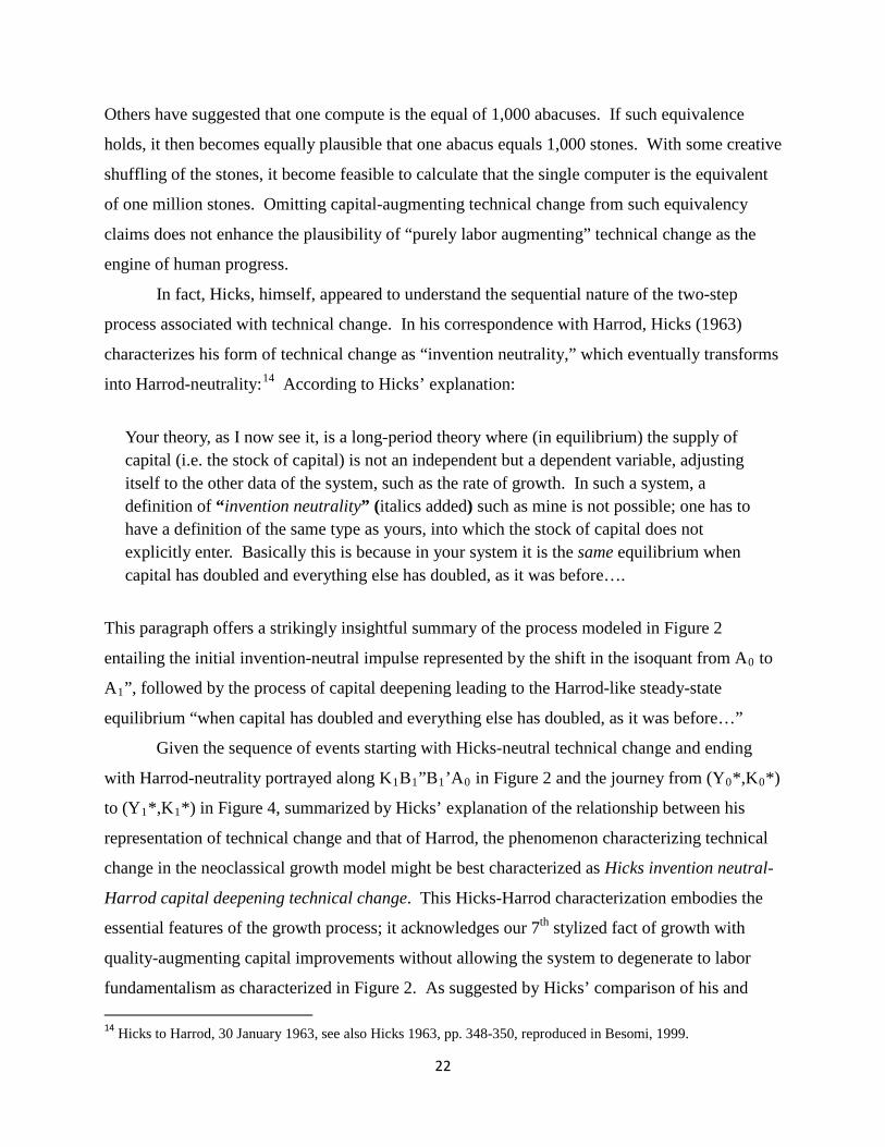
In fact, Hicks, himself, appeared to understand the sequential nature of the two-step

process associated with technical change. In his correspondence with Harrod, Hicks (1963)

characterizes his form of technical change as “invention neutrality,” which eventually transforms

into Harrod-neutrality:14 According to Hicks’ explanation:

Your theory, as I now see it, is a long-period theory where (in equilibrium) the supply of capital (i.e. the stock of capital) is not an independent but a dependent variable, adjusting itself to the other data of the system, such as the rate of growth. In such a system, a definition of “invention neutrality” (italics added) such as mine is not possible; one has to have a definition of the same type as yours, into which the stock of capital does not explicitly enter. Basically this is because in your system it is the same equilibrium when capital has doubled and everything else has doubled, as it was before….

This paragraph offers a strikingly insightful summary of the process modeled in Figure 2

entailing the initial invention-neutral impulse represented by the shift in the isoquant from A0 to

A1”, followed by the process of capital deepening leading to the Harrod-like steady-state

equilibrium “when capital has doubled and everything else has doubled, as it was before…”

Given the sequence of events starting with Hicks-neutral technical change and ending

with Harrod-neutrality portrayed along K1B1”B1’A0 in Figure 2 and the journey from (Y0*,K0*)

to (Y1*,K1*) in Figure 4, summarized by Hicks’ explanation of the relationship between his

representation of technical change and that of Harrod, the phenomenon characterizing technical

change in the neoclassical growth model might be best characterized as Hicks invention neutral-

Harrod capital deepening technical change. This Hicks-Harrod characterization embodies the

essential features of the growth process; it acknowledges our 7th stylized fact of growth with

quality-augmenting capital improvements without allowing the system to degenerate to labor

fundamentalism as characterized in Figure 2. As suggested by Hicks’ comparison of his and 14 Hicks to Harrod, 30 January 1963, see also Hicks 1963, pp. 348-350, reproduced in Besomi, 1999.

23

Harrod’s versions of technical change, for the purpose of understanding economic growth, it is

not sufficient to characterize technical change simply as a shift in an isoquant (e.g., Hicks’

invention neutrality), nor as the end-state of the capital deepening process in which the technical

change becomes absorbed into the relevant factors of production. Both are essential and

inseparable for understanding the impact of technological change on growth. Hence, the term

Hicks-Harrod is appropriate for understanding the cumulative nature of technical change – in the

case of Eq. (7b), both the invention neutrality, gH, and the capital deepening, α/(1-α), that

together consummate in the cumulative impact of 1/(1-α).

One of the several advantages of the Hicks-Harrod paradigm relative to the standard

Harrod paradigm is that, while the latter confounds the exogenous and endogenous elements of

the growth process, the Hicks-Harrod paradigm not only demonstrates the inseparability of

technical change and capital deepening, it clearly distinguishes their respective contributions: the

exogenous component in the form of Hicks invention neutrality from the endogenous component

– the subsequent capital deepening that converges to Harrod neutrality. As such, this preferred

characterization of technical change is transformative in that it delineates the exogenous

phenomenon as invention based, potentially reconstituting the role of innovation as externally-

created technical change that embodies certain of the characteristics of a public good. At the

same time, the Hicks-Harrod sequence clearly endogenizes the phenomenon of Harrod-neutral

capital-deepening, associated with the multiplier, i.e., α/(1-α), involving the adoption and

propagation of new rounds of invention through the investment process. The multiplier effect

opens the door for a relatively uniform set of technologies to be accessed, diffused, and absorbed

to different degrees by different economies.

Here we formally disaggregate the Harrod vs. Hicks technology multipliers into two

separate and discrete events. For labor-augmenting technical change, the first event is the direct

impact of technical change on the effective supply of labor. The second is the capital deepening

that ensues as a result of the endogenous increase in the demand for capital, whose marginal

product now exceeds the rental cost of capital and has been enabled in part by the increase in

output and the outward shift in the savings supply schedule. These distinct channels of technical

change, summing to the total impact, are shown in the following table.

24

For the Hicks case, the neutral technical change raises the effective supplies of both

capital and labor in direct proportion to gH resulting in an immediate increase in the effective

supplies of labor and capital, as well as output. As shown in the last column of the table, for

both the Harrod and Hicks cases, capital’s output elasticity is α. However, as derived in Eqs. (3a)

and (7a), we see that whereas (dk/k)/(dA/A) = 1 for the Harrod case, for the Hicks case it is 1/(1-

α), resulting from the fact that, in contrast with the Harrod case, both the quality and marginal

products of both labor and capital rise directly from the Hick’s neutral technical advance. Hence,

the total multiplier effect for the Hicks case is [α + (1-α)]{1 + α[1/(1-α)]} = 1/(1-α).

Seemingly, the link between the exogenous and endogenous phases of growth as captured

by the Hicks-Harrod invention-capital deepening paradigm has been lost on the growth (and

development) accounting field of research. In his “development accounting” of differences in

the sources of income and growth spanning 94 countries, Caselli (2004, p. 4) writes:

“Furthermore, it (development and growth accounting) has nothing to say on the way factor

accumulation and efficiency influence each other, as they most probably do.” Hopefully, the

distinction between the Harrod and Hicks technology multipliers offers helpful insight regarding

the reasons for this theoretical and empirical not to be so disconnected in the literature.

The differences in the Harrod and Hicks technology multipliers are further illuminated by

the Mankiw, Romer, Weil (MRW, 1992) human-capital augmented Solow model in which α and

β represent the output elasticities of physical capital and human capital respectively, leaving 1-α-

β to represent the output contribution of unschooled, physical labor. In the MRW model, with

purely labor augmenting technical change, the direct impact of gA is limited to augmenting the

effective supply of unskilled or physical labor accounting for (1-α-β)% of economy. It then falls

on this portion of the unschooled economy to motivate the phenomenon of capital deepening

across the remaining (α+β)% of the economy. Whereas for the labor-augmenting case,

broadening the measure of capital has no effect on the multiplier effect of labor-augmenting

Table 1. Comparing labor-augmenting and Hicks-neutral technical change Total impact Direct impact effect Induced capital-deepening (dy/y)/(dA/A) dA/A [(dy/y)/(dk/k)]*[(dk/k)/(dA/A)]

Labor-augmenting 1 1-α α*1 Hicks-neutral (σ=1) 1/(1-α) 1 α*1/(1-α)

25

technical change, for the Hicks-Harrod case, the addition of human capital, expands the total

multiplier to [1/(1-α-β)] and the capital-deepening multiplier to [(α+β)/(1-α-β)]. A further

insight that can be garnered from the MRW (1992) model. As shown in their Eq. (11), whereas

the addition of β expands the measure of broad capital, thereby increasing the multiplier effect of

changes in s, n, gA, and δ on deviations from the steady state, it has no effect of the multiplier

effect of gA in the steady state, again demonstrating the dependence of capital deepening on the

nature of the initial technical change.

Two summary examples can hopefully extend our appreciation of the potential power of

the Hicks-Harrod technology multiplier as a vehicle for understanding differences in country

growth performances. In their review of the history of higher education in the U.S., Thelin et al.

(undated) characterize the period 1945-1970 as “the golden age” of American higher education

in which the GI bill and baby boom led to a dramatic surge in the proportion of the U.S.

workforce acquiring post-secondary education. Gao and Jefferson (2007) characterize this

period of one of “S&T takeoff” for the U.S. and other large OECD economies during which

R&D expenditure as a share of GDP rose rapidly from less than 1% to the vicinity of 2.5%.

Together, the surge in enrollments in higher education and R&D intensity during the 1945-1970

period greatly increased the weight of broad capital in the American economy and the multiplier

effect of technical change.

China during 1980-2015 may be a yet more dramatic illustration. During this period,

even as rates of savings hovered in the vicinity of 50% so as to foster the surge of investment in

infrastructure, factories and services, including a dramatic upswing in secondary and post-

secondary education, thus much increasing the quantities of physical and human capital, the

returns to both public and private investment increased measurably relative to the socialist

period.15 During the reform period in China, α+β, the measure of broad capital’s share,

including human capital’s output elasticity, β, grew measurably while (1-α-β), the factor income

share of unschooled labor diminished.

For both the U.S. and China, these respective eras of rapid growth were periods during

which the share of broad capital, particularly human capital, rose substantially thus expanding

the Hicks-Harrod technology multiplier. Nonetheless, from the perspective of Kaldor’s stylized

15 See, for example, Naughton (2007, Fig. 8.5), who shows the returns to education in urban China rising from 4% per annum in 1988 to 10% in 1999.

26

facts, including the relative constancy of capital and labor’s factor income share, the combined

expansion of β and shrinkage of 1-α-β may not have significantly altered labor’s overall share of

national income. The key insight is that with the introduction of the Hicks-Harrod multiplier, the

neoclassical model acquires the ability to explain differences in levels and rates of growth of

living standards both across and within national economies.

In the next section, we reformulate the steady-state equation to be consistent with Hicks-

Harrod technical change.

5. Revisiting the steady-state equation

As derived in Section 2, the standard representation of the neoclassical growth steady-

state equation under the assumption of purely labor-augmenting technical change is K/Y = k/y =

k~/y~ = s/(n+gA+δ). One feature that unites all four of the steady-state parameters – s, n, gA, and

δ – is that in the steady-state context each is factor-biased. The rates of savings and depreciation

directly affect the rate of accumulation of the net capital stock. The rates of population and

labor-augmenting technical change both augment the effective supply of labor. The parameters s

and δ enter into the equation of motion; n and g define the steady-state rates of growth of capital

and labor.

We now show the implications for the steady state equation of adopting the Hicks-Harrod

version of the neoclassical model rather than the pure Harrod version. In contrast to the

conventional derivation of the steady state equation in which Harrod-neutral technical change is

factor-biased, when our measure of Hicks-neutral technical change, gH, is symmetrically applied

across factors as disembodied technical change, it will exert equivalent effects on capital, labor

and output. To demonstrate this, we write the capital-augmenting version of the equation of

motion:

dK = sY + (gH – δ)K, (11a)

where gH represents the neutral innovation that augments the quality and effective supply of

capital even as it is being depreciated by δ. Hence (gH – δ) represents the rate of net depreciation

27

of the capital stock. Eq. (11a) can be rearranged in the usual manner, so that by dividing through

by K,, Eq. (11a) transforms to:

dK/K, = sY/K, + gH – δ (11b)

Given that in the steady state the capital stock grows at the same rate as the effective supply of

labor, i.e., n + gH, we equate the two:

dK/K, = sY/K, + gH – δ = n + gH. (11c)

Therefore:

K/Y = s/(n – δ). (11d)

For the conventional application of technical change, i.e., as fully disembodied, then Hicks-

Harrod neutrality acts on all factors in a symmetric and equi-proportional manner, so as to be

factor neutral, enabling the measure of technical change to be excluded from the steady state.

Thus, the full measure of our reformulated model of neoclassical growth is:

gy = [1/(1-α)]gH + [α/(1-α)]V^ (12a)

V = K/Y = k~/y~ = s/(n+δ). (12b)

We can identify the mathematical relationship between the steady-state parameters, s, n,

and δ and the economy’s factor intensity by dividing y = Akα by A. which gives

y~ = k~α. (13)

Eq. (11) can be rewritten as:

k~/y~ = k~1-α = s/(n+δ) (14a)

and transformed to:

k~ = K/(AL) = [s/(n+δ)]1/(1-α). (14b)

28

Eq (14b) shows the effect of a change in the steady-state parameters on the ratio of the

factor-income shares in the steady state when A = MPL = w and the interest rate, r, is fixed.

Hence, Eq. (14b) can be written as:

α/(1-α) = [s/(n+δ)]1/(1-α) (14c)

Given that with Hicks-neutral technical change, α/(1-α) determines the extent of capital

deepening following a round of Hicks invention neutral technical change – thus engendering a

total multiplier effect of 1/(1-α) – Eq. (14c) now shows that an increase in the savings rate – or

reduction in either the rate of population growth or depreciation – increases the multiplier effect

of Hicks-neutral technical change.

Given Solow’s finding, which was orthogonal to that of Harrod-Domar, that the saving

rate has no effect on long-run growth, this result is of particular consequence. Furthermore, the

causal relationship between the rate of population growth, capital deepening, and the sustained

growth of living standards, may help to explain the association over the 20th Century between the

Demographic Transition in the OECD countries and the acceleration of living standards as well

as the tendency for the East Asian economies, distinguished by their high and rising rates of

savings and declines in fertility, to have enjoyed surging living standards during the latter half of

the 20th Century carrying over to the current period.16 The Hicks-Harrod proposition is that

changes in key economic/policy parameters, notably s and n, not only have transitory

implications for the rate of growth of output per capita, as shown by Solow, by affecting the

capital-deepening multiplier, α/(1-α), they also exert sustained effects on the steady-state

balanced growth path.

In the next section, we discuss the implications of production technologies for which σ ≠

1 for modeling the bias of technical change and the technology multiplier.

6. Uzawa, CES, and the substitution elasticity

16 This speculation is not intended to diminish the recognition that rising living standards, particularly female labor force participation and rising educational levels, have also been a critical driver of declining fertility (see, for example, T.P Schultz, 1981.

29

Before examining the implications for the steady state balanced growth path of an

economy in which the substitution elasticity deviates from unity, we review the arguments for

retaining the assumption of a Cobb-Douglas production technology in which σ =1:

1. The Cobb-Douglas technology is consistent with the Kaldor Facts, i.e., relatively stable

factor income shares over long-periods of time.

2. So as to avoid α drifting toward 0 or 1 within the steady state, for purely labor-augmenting

technical change, the steady state condition of a fixed capital-output ratio requires σ = 1.

Furthermore, notwithstanding the mistaken argument common in the literature that the

Cobb-Douglas technology with σ = 1 is required for Hick-neutrality but not Harrod-

neutrality, the same literature generally continues to use the solely labor-augmented version

of the Cobb-Douglas functional form.

3. The indifference of the labor-augmenting paradigm to the presence of capital, including the

K-Y ratio, as well as the indifference of its technology multiplier to the magnitudes of σ and

α, does not recommend it as the basic engine of economic growth. These conditions, as

well as the inability of purely labor-augmenting technical change to explain progressive

improvement in the quality of capital, readily support the misgivings of Solow and

Acemoglu.

4. Steady states may come and go. Arguably, the condition that σ approximate unity should

be a requirement of the steady state. In time series data, most documented deviations from

stationary factor income shares have themselves been transitory. The requirement that in

the neighborhood of a true steady state, the economy’s substitution elasticity approximate

unity is a small price to pay for the admission of capital-augmenting technical change.

5. Finally, the Cobb-Douglas with Hicks-neutral technical change may have been

relegated to the dust bin of history due to an error in Solow’s original 1956 article in which,

for Hicks-neutrality in the Cobb-Douglas context, he miscalculated the steady state rate of

growth of the effective labor supply. Due to this miscalculation, Solow mistakenly

concluded that with the Hicks version of the Cobb-Douglas, the K-L and K-Y ratios would

become explosive, thus defying the existence of a steady state.17 Had Solow validated the

existence of a steady state with Hicks neutral technical change, our representation of his

model today may be far different.

17 See Solow (1956), pp. 85-86.

30

Notwithstanding these arguments for adopting the basic model of neoclassical growth as that

with Hicks-neutrality within a Cobb-Douglas function, including the addition of the steady state

condition, σ=1, if needed, we examine more deeply the case in which σ ≠ 1.

In their paper in which they develop the Non-Identification Theorem, Diamond,

McFadden, and Rodriguez (1978) demonstrate that within the context of a given time series of

the growth of output per capita, the underlying substitution elasticity and capital-labor-factor-

augmenting rates of change can assume a range of different, but empirically unobservable,

values. While Diamond et al do not specifically focus on the neoclassical steady state, we can

use their analytical framework to can confirm the known case in which Hicks-neutral technical

change is compatible with σ = 1, as well as the case, contrary to the strong form of Uzawa (1961),

in which neutral factor-augmenting technical change is compatible with production technologies

for which σ ≠ 1. The intuition for this result is that whereas the initial surge of Hicks invention

neutrality may be equal across capital and labor, the impacts that each has on the degree of

capital augmentation differ, so as to compensate for the absence of factor neutrality in the

substitution elasticity (i.e., σ = 1). The non-neutralities that result in the growth process from σ ≠

1 and the mix of factor-augmenting bias can be mutually offsetting.

To demonstrate the various cases that frame their Non-Identifiability Theorem, Diamond

et al differentiate the classical production function, Y = f(AK,BL,t) under constant returns and

competition, in which:

gy = output per capita k = the capital-labor ratio v = y/k (designated previously as K/Y = V) α = capital’s output elasticity s = ratio of factor income shares α/(1-α) 1/σ = dlnp/dlnk p = w/r, the wage-rental ratio A(t) = capital-biased technical change B(t) = labor-biased technical change x = capital-labor ratio in efficiency units, i.e., kA(t)/B(t) T(k,t) = ft/f,

Their calculations result in the following growth equation shown in Diamond et al, Eq. (10a):18 18Derived by Diamond (1965). The caret, ^, represent a rate of growth.

31

gw = B^ + (α/(1-α)(1/σ)A^ - (s/σ)v^.

Although Diamond et al do not relate their results to the Solow steady state, we can

readily see that by imposing the competitive and steady state conditions, x^ = v^ = r^ = 0, so that

s^ = 0 and gy = gw,19 their Eq. (10a) can be written as gy = B^ + (s/σ)A^. Furthermore, we

impose the restriction of Hicks invention neutrality, so that B^ = A^ = gH. As a result:

gY = {1 + [α/(1-α)](1/σ)}gH. (15)

We first note from Eq. (15) that for the case in which σ = 1, i.e., the Cobb-Douglas case,

we obtain the previously derived technology multiplier, i.e., 1(1-α). To help understand the

intuition of the general result in Eq. (15), we have formulated Fig. 5, which shows a comparison

of two economies with different production technologies and different substitution elasticities.

The first is initially represented by the isoquant Y0’Y0’ with σ = 2; for the other, Y0”Y0”, σ = ½.

Assuming α = ½ and gH = 1, the technology multiplier for Y0’ is 3/2, resulting in a shift along

the fixed K/L ratio from A0 to A1’. As a result, Y/L grows by 150%,. Since Y is fixed, the

increase results exclusively from an increase in the efficiency measure of labor, while labor’s

physical measure declines by 2/3. At the same time, the w/r ratio – with r fixed, it is simply the

wage – also rises by 150%, as shown by the increase in the slope of the w/r factor price line

from P0 to P1’. Since r^ = K^ = 0 and gp = gk, reflecting the reduction in the work force, thus

keeping capital and labor’s income shares and K/Y unchanged, the growth achieved by the shift

from A0 to A1’ is consistent with the steady state.

At the same time, for the economy represented by Y0”Y0”, for which σ = ½, the

equivalent 1% increase in gH results in the shift from A0 to A1”, which is twice the distance

along K/L relative to the increase in gw for the economy for which σ = 2. As a result of the

larger technology multiplier associated with σ = ½ as compared with σ = 2, the increase in the

wage as shown by the price line P1” exactly compensates for the relative reduction in the

remaining quantity of physical labor, shown at L0”, thus holding the economy’s labor income

share fixed. 19This case is consistent with case 2a in Table 2 (“Bounds on the elasticity of substitution implied by factor augmenting technical progress”) in Diamond, McFadden, and Rodriguez.

32

Given Eq. (15), we can determine that [∂(gY/gH)/(gY/gH)]/(∂σ/σ) = -sσ-1/(1 + sσ-1) < 0, so

that for α = ½ and σ = 1 a 1% increase in σ results in a 0.5% reduction in the magnitude of the

technology multiplier. For α = ½ and σ = 2, the associated reduction in the growth of output per

capita associated with a given gH is 0.33%.

We can also see from Eq. (15), that [∂(gY/gH)/(gY/gH)]/(∂s/s) = (s/σ)/(1+s/σ) > 0. For σ =

1 and s = ½ (α = 1/3), a 1% increase in s translates to a 0.33% increase in the technology

multiplier. For s = 2 (α = 2/3), the 200% fold increase in s, (i.e., an increase in α from 1/3 to 2/3),

results in a 167% increase in the magnitude of the multiplier.

At first glance, it may seem counter intuitive that for a given level of invention neutrality,

an economy evidencing less substitutability – more rigidity – between capital and labor should

yield higher growth and wages than one in which there would appear to be less flexibility. The

relevant condition, however, is that in the economy in which there is less substitutability and

more complementarity between capital and labor, capital deepening has the effect of elevating

wages and incomes to a greater degree than the economy in which capital-labor substitution is

more pervasive, thus financing greater investment and capital deepening.

Unlike the standard neoclassical model in which an economy’s substitution elasticity is to

be taken as purely exogenous datum embedded in the DNA of a nation’s production technology,

in the generalized version of our technology multiplier, in which the multiplier is highly

responsive to the value of σ, the determinants of an economy’s substitution elasticity value

warrant serious attention.20 Clearly, over time, substitution possibilities change, as presently

there are, for example, with mining, in which the growth of extraction technologies presents a far

wider set of production possibilities combining capital and labor than had existed in the 18th

Century. Today, across countries, within manufacturing, the continuum of capital-labor

substitution possibilities spans physical-labor to robotic-centered assembly across many similar

products. At the same time, within economies, limited degrees of substitutability may be

available for many products, such as pharmaceuticals, semiconductors, and aircraft construction.

As shown in this section, by understanding differences within and across economies in prevailing

factor substitution elasticities, we might begin to more deeply and accurately assess the impact of 20 Hicks (1932, p. 132), for example believed that the substitution elasticity was likely to fall over time: “If capital is increasing more rapidly than the supply of labour (and it may fairly be supposed that this has generally been the case in modern English history), a tendency towards a diminished elasticity of substitution will generally set in as capital grows. This diminution may be counteracted by invention – it is conceivable that it might be counteracted indefinitely – but clearly invention has a progressively harder task as the process goes on. “

33

the relationship between the evolution of production technologies – composition as well as

aggregate measures – and the sources of long-run growth.

Absent a full-fledged theory and empirical test of the factors determining the magnitude

and change in values of σ, revisiting Argument #4 at the beginning of this section, characterizing

the steady state as that in which σ = 1 and roughly constant may be an entirely reasonable and

practical assumption, particularly if, according to Diamond et al (1078), we are unable to

effectively distinguish between the contributions that σ and technical change make to the

appearance in which the economy’s factor income shares are fixed as if the economy were

functioning in accord with a unitary substitution elasticity.

7. Conclusions and further thoughts

This paper formulates a more accurate, complete, and potentially more powerful account

of the process of long-run economic growth than that represented by standard accounts of the

neoclassical growth model. The paper highlights various limitations and contradictions within

the conventional model and inconsistencies with real-world growth phenomena. These include

the following five shortcomings of the existing model. That model:

provides no vehicle for the quality of capital to improve over time – and is therefore

nonsensical, to the extent that its result can be achieved without the existence of capital;

does not represent technical change in the usual sense in which the microeconomics

literature models technical change;

fails to sufficiently appreciate the role of capital, both as a vehicle for technical change and

an avenue for capital deepening, that greatly multiplies the impact of exogenous technical

change; i.e., the impact of labor-augmenting technical change is indifferent to α, the

marginal product of capital and the slope of the intensive production function.

offers a paucity of insight concerning differences in both levels and rates of growth of

living standards among and within countries; and

obfuscates the respective sources of exogenous efficiency gains and endogenous factor

accumulation thereby severely limiting the possibilities for a more integrated, unified

theory and application of neoclassical growth, endogenous growth, and growth accounting.

34

Why did growth theory go down this road? The standard representations of neoclassical

growth as formulated by Solow, Uzawa and others, are giant theoretical innovations creating

shoulders on which many have subsequently stood. Yet, arguably, along the way, the theory has

veered off track. Of note are the following errors and oversights. Kaldor omitted a key stylized

fact from his list – that of progressive quality improvements in capital. Solow mistakenly

nullified the consistency of Hicks-neutral technical change with the final steady-state growth

equilibrium. The Uzawa Theorem more firmly hedged in our appreciation of the array of

possibilities for technical change, instead focusing our pre-occupation on a final-state

equilibrium in which the impetus to growth appears to be an entirely externally-generated, labor-

centered phenomenon that magically appears as manna from heaven. Finally, analysts have

misinterpreted the role of σ in framing steady state growth, without appreciating the fact that in

order to conform with the requirements of the steady state, labor-augmenting technical change

either requires that σ = 1 or that it be paired with capital-augmenting technical change, with or

without σ = 1. These conditions that are no less restrictive than those imposed on Hicks-

neutrality. This paper seeks to explicitly address and remedy this string of interlocking errors

and oversights.

Most likely, these shortcomings arise from a certain fetish that we economists all share

for long-run gratification. In the case of the neoclassical growth model this pre-occupation

drives us to devise various creative formulations of the nature of growth in its steady state,

thereby suppressing attention to the essential details of the growth process. Most importantly the

lesson is that growth is a process that involves multiple economic activities and interactions that

cannot be facilely reduced to a single outcome or stationary diagram. Within the broader field of

growth, the narrow focus on the finality of steady-state convergence has created an unfortunate

separation, even divorce, between neoclassical growth theory, endogenous growth, and growth

accounting. The formulation devised in this paper incorporating both Hicks invention neutrality

and Harrod capital deepening will hopefully open a path to the integration of these disparate

fields of study of growth.

There is a certain urgency to the message of this paper. Eighty years ago, Ronald Coase

stuck his finger in the eye of economists and our discipline by arguing that by embracing the

tenets of the pure neoclassical model – complete, perfect, and frictionless markets and full

information – there was no space in our idealized model for something as commonplace as the

35

firm. As teachers today, we would never walk into the classroom and preach to our students a

doctrine that has such ridiculous implications – or at least not finish the semester letting them

venture into the outer world vulnerable to the ridicule that such a worldview would invite.

Likewise, we should feel some discomfort in setting forth a model of economic growth in which

we represent human creativity as “purely labor augmenting” thus disallowing space for

smartphones or air travel, while also propagating a model in which various logical

inconsistencies arise as we attempt to justify this misplaced model of human progress.

36

Bibliography

Acemoglu, Daron, 2000. “Labor- and Capital Augmenting Technical Change, NBER Working Paper 7544 http://www.nber.org/papers/w7544. Acemoglu, Daron, 2009. Introduction to Modern Economic Growth, Princeton University. Aghion and Howitt, 2007. “Capital, innovation, and growth accounting,” Oxford Review of Economic Policy, Volume 23, Number 1, 2007, pp.79–93 Barro, R.J. and X. Sala-i-Martin, 1995. Economic Growth, New York, McGraw-Hill. Besomi, Daniele, 1999. “Harrod on the classification of technological progress. The origin of a wild-good chase,” BNL Quarterly Review, no. 208, March 1999. Brada, Josef C.,” (2013) The distribution of income between labor and capital is not stable: But why is that so and why does it matter?, Econ.Systems, http://dx.doi.org/10.1016/j.ecosys.2013.04.001 Caselli, Francesco, (draft, 2004). “Accounting for Cross-Country Income Differences,” published in The Handbook of Economic Growth, edited by P. Aghion and S. Durlauf, Ch. 9, 2014. Elsevier. Coase, Ronald, 1937. Economica, New Series, Vol. 4, No. 16. (Nov., 1937), pp. 386-405. Diamond, Peter, 1965, "Technical Change and the Measurement of Capital and Output," Review of Economic Studies, XXXII, October 1965, 289-298. Diamond, Peter, McFadden, Daniel, Rodriguez, Miguel, 1978., “Measurement of the Elasticity of Substitution and the Bias of Technical Change,”, in M. Fuss and D. McFadden, Production Economics: A Dual Approach in Theory and Applications, Ch. 4, Vol. 2, Amsterdam: North Holland,. Domar, Evsey, 1946. "Capital Expansion, Rate of Growth, and Employment,” Econometrica, 14 (2): 137–147. Gao, Jian and G. H. Jefferson, (2007). “Science and Technology Takeoff in China? Sources of Rising R&D Intensity,” 2007, Asia Pacific Business Review, 13,3:357-371. Hahn, F.H. and Matthew, R.C.O., 1964. “The Theory of Economic Growth: A Survey,” The Economic Journal, Vol. 74, No. 296: pp. 779-902. Harrod, Roy F. 1961, “The ‘neutrality’ of improvements,” The Economic Journal, 71: 300-304. Hicks, John Richard, 1963 (1932). The Theory of Wages, Macmillan, London, 2nd edition.

37

Jones, Charles I. and Dean Scrimgeour, 2005. “The Steady-State Growth Theorem: Understanding Uzawa (1961)”, August 16, 2005, https://www.aeaweb.org/assa/2006/0106_1430_0702.pdf Jones, Charles I. and Romer, Paul M., 2010. “The New Kaldor Facts: Ideas, Institutions, Population, and Human Capital,” American Economic Journal: Macroeconomics 2(1), 224-45. Jones, Charles and Dietrich Vollrath, 2013. Introduction to Economic Growth, W.W. Norton & Co., New York and London. Jones, Hywel, 1975. Modern Theories of Economic Growth, Thomas Nelson and Sons, Ltd. Kaldor, Nicholas, 1961, “Capital Accumulation and Economic Growth,” in F. A. Lutz and D. C. Hague, editors, The Theory of Capital. New York: St. Martin's Press. Kennedy Charles (1964), Induced Bias in Innovation and the Theory of Distribution, The Economic Journal, Vol. 74, No. 295, pp. 541-547. Keynes, John M, 1936. The General Theory of Employment, Interest and Money. London: Macmillan (reprinted 2007). Mankiw, Romer, Weil. 1992. “A Contribution to the Empirics of Economic Growth,” Quarterly Journal of Economics. Masanjala, Winford, H. and Chris Papagengiou, 2003. “The Solow Model with CES Technology: Nonlinearities and Parameter Heterogeneity, March 2003. Naughton, Barry (2007). The Chinese Economy: Transitions and Growth, MIT Press, Cambridge, MA. Nordhaus, William, 1992. "Lethal Model 2: The Limits to Growth Revisited." Brookings Papers on Economic Activity, 2: 1-43. Romer, Paul, 1990, “Endogenous Technical Change,” Journal of Political Economy, 98,5: Romer, Paul, 1994b. “Origins of Endogenous Growth,” Journal of Economic Perspectives, 8,1:3-22. Samuelson, Paul, “A Theory of Induced Innovations Along Kennedy-Weisacker Lines” Review of Economics and Statistics, XLVII (1965), 444-464. Schultz, T. Paul, 1981. The Economics of Population, Addison-Wesley, Boston. Solow, Robert M., 1956. “A Contribution to the Theory of Economic Growth.” Quarterly Journal of Economics 70 (1): 65–94.

38

Solow, Robert M., 1957. “Technical Change and the Aggregate Production Function,” Review of Economics and Statistics, pp. 312-20. Solow, Robert M., 2000. Growth Theory: An Exposition, Oxford University Press, New York. Solow, Robert M., 1988. “Growth Theory and After,” The American Economic Review, Vol. 78, No. 3 (Jun., 1988), pp. 307-317. Thelin, John R., Jason R. Edwards, Eric Moyen, Joseph B. Berger, and Maria Vita Calkins (undated), “Higher Education in the United States - HISTORICAL DEVELOPMENT, SYSTEM,” http://education.stateuniversity.com/pages/2044/Higher-Education-in-United-States.html#ixzz4VYGLm2qh. Uzawa, Hirofumi, 1961. “Neutral Inventions and the Stability of Economic Growth,” Review of Economic Studies, 28: 117-124.

39

Figure 1

Jones and Vollrath (2013)

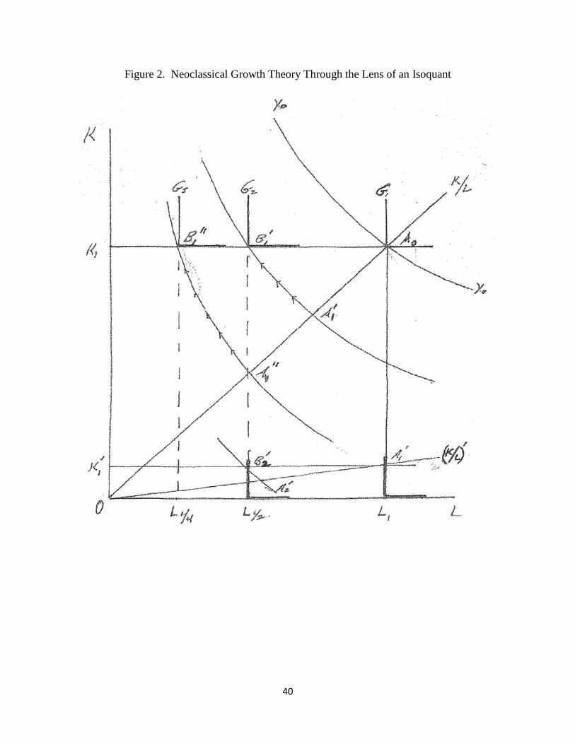
40

Figure 2. Neoclassical Growth Theory Through the Lens of an Isoquant

41

Figure 3. A typology of technical change

Acemoglu (2009), p. 59.

42

Figure 4. The Hicks invention neutrality-Harrod capital deepening version of growth

43

Fugure 5. Implications of σ for the Technology Multiplier in the Steady State