REFERENCE DESIGN REPORT ILC Global Design Effort and … · INTERNATIONALLINEARCOLLIDER...
151
INTERNATIONAL LINEAR COLLIDER REFERENCE DESIGN REPORT ILC Global Design Effort and World Wide Study AUGUST, 2007
Transcript of REFERENCE DESIGN REPORT ILC Global Design Effort and … · INTERNATIONALLINEARCOLLIDER...

INTERNATIONAL LINEARCOLLIDER
REFERENCE DESIGNREPORT
ILC Global Design Effort and
World Wide Study
AUGUST, 2007

Volume 1: EXECUTIVE SUMMARY
Editors:
James Brau, Yasuhiro Okada, Nicholas Walker
Volume 2: PHYSICS AT THE ILC
Editors:
Abdelhak Djouadi, Joseph Lykken, Klaus Monig
Yasuhiro Okada, Mark Oreglia, Satoru Yamashita
Volume 3: ACCELERATOR
Editors:
Nan Phinney, Nobukazu Toge, Nicholas Walker
Volume 4: DETECTORS
Editors:
Ties Behnke, Chris Damerell, John Jaros, Akiya Miyamoto

Reference Design Report Physics at the ILC
August 2007ILC-REPORT-2007-001
international linear collider

AAI-PUB-2007-002BNL-79150-2007CERN-2007-006 CHEP A07-001 (CHEP/KNU) CLNS 07/1991Cockcroft -07-04DESY 07-046FERMILAB-TM-2382-AD-CD-DO-E-FESS-TDJAI-2007- 001JINR Dubna-E9-2007-39JLAB-R-2007-01KEK Report 2007-2LBNL- 62867LNF-07/9(NT)SLAC-R-857
ISSN 0007-8328ISBN 978-92-9083-299-7
http://www.linearcollider.org
P.O. Box 500Batavia, IL60510USA
1-1 Oho,Tsukuba, Ibaraki305-0801Japan
DESY-FLCNotkestrasse 85,22607 HamburgGermany

Volume 2: PHYSICS AT THE ILC
Editors:
Abdelhak Djouadi, Joseph Lykken, Klaus Monig
Yasuhiro Okada, Mark Oreglia, Satoru Yamashita


List of Contributors
Gerald Aarons203, Toshinori Abe290, Jason Abernathy293, Medina Ablikim87,Halina Abramowicz216, David Adey236, Catherine Adloff128, Chris Adolphsen203,
Konstantin Afanaciev11,47, Ilya Agapov192,35, Jung-Keun Ahn187, Hiroaki Aihara290,Mitsuo Akemoto67, Maria del Carmen Alabau130, Justin Albert293, Hartwig Albrecht47,
Michael Albrecht273, David Alesini134, Gideon Alexander216, Jim Alexander43,Wade Allison276, John Amann203, Ramila Amirikas47, Qi An283, Shozo Anami67,B. Ananthanarayan74, Terry Anderson54, Ladislav Andricek147, Marc Anduze50,
Michael Anerella19, Nikolai Anfimov115, Deepa Angal-Kalinin38,26, Sergei Antipov8,Claire Antoine28,54, Mayumi Aoki86, Atsushi Aoza193, Steve Aplin47, Rob Appleby38,265,
Yasuo Arai67, Sakae Araki67, Tug Arkan54, Ned Arnold8, Ray Arnold203,Richard Arnowitt217, Xavier Artru81, Kunal Arya245,244, Alexander Aryshev67,
Eri Asakawa149,67 , Fred Asiri203, David Asner24, Muzaffer Atac54, Grigor Atoian323,David Attie28 , Jean-Eudes Augustin302, David B. Augustine54, Bradley Ayres78,
Tariq Aziz211, Derek Baars150, Frederique Badaud131, Nigel Baddams35,Jonathan Bagger114, Sha Bai87, David Bailey265, Ian R. Bailey38,263, David Baker25,203,Nikolai I. Balalykin115, Juan Pablo Balbuena34, Jean-Luc Baldy35, Markus Ball255,47,
Maurice Ball54, Alessandro Ballestrero103, Jamie Ballin72, Charles Baltay323,Philip Bambade130, Syuichi Ban67, Henry Band297, Karl Bane203, Bakul Banerjee54,
Serena Barbanotti96, Daniele Barbareschi313,54,99, Angela Barbaro-Galtieri137,Desmond P. Barber47,38,263, Mauricio Barbi281, Dmitri Y. Bardin115, Barry Barish23,59,Timothy L. Barklow203, Roger Barlow38,265, Virgil E. Barnes186, Maura Barone54,59,
Christoph Bartels47, Valeria Bartsch230, Rahul Basu88, Marco Battaglia137,239 ,Yuri Batygin203, Jerome Baudot84,301, Ulrich Baur205, D. Elwyn Baynham27,
Carl Beard38,26, Chris Bebek137, Philip Bechtle47, Ulrich J. Becker146, Franco Bedeschi102,Marc Bedjidian299, Prafulla Behera261, Ties Behnke47, Leo Bellantoni54, Alain Bellerive24,
Paul Bellomo203, Lynn D. Bentson203, Mustapha Benyamna131, Thomas Bergauer177,Edmond Berger8, Matthias Bergholz48,17, Suman Beri178, Martin Berndt203,
Werner Bernreuther190, Alessandro Bertolini47, Marc Besancon28, Auguste Besson84,301,Andre Beteille132, Simona Bettoni134, Michael Beyer305, R.K. Bhandari315,
Vinod Bharadwaj203, Vipin Bhatnagar178, Satyaki Bhattacharya248 ,Gautam Bhattacharyya194 , Biplob Bhattacherjee22, Ruchika Bhuyan76, Xiao-Jun Bi87,
Marica Biagini134, Wilhelm Bialowons47, Otmar Biebel144, Thomas Bieler150,John Bierwagen150, Alison Birch38,26, Mike Bisset31, S.S. Biswal74, Victoria Blackmore276,
Grahame Blair192, Guillaume Blanchard131, Gerald Blazey171, Andrew Blue254,Johannes Blumlein48, Christian Boffo54, Courtlandt Bohn171,∗, V. I. Boiko115,
Veronique Boisvert192, Eduard N. Bondarchuk45, Roberto Boni134, Giovanni Bonvicini321,
ILC-Reference Design Report II-i

Stewart Boogert192, Maarten Boonekamp28, Gary Boorman192, Kerstin Borras47,Daniela Bortoletto186 , Alessio Bosco192, Carlo Bosio308, Pierre Bosland28, Angelo Bosotti96,Vincent Boudry50, Djamel-Eddine Boumediene131, Bernard Bouquet130, Serguei Bourov47,
Gordon Bowden203, Gary Bower203, Adam Boyarski203, Ivanka Bozovic-Jelisavcic316 ,Concezio Bozzi97, Axel Brachmann203, Tom W. Bradshaw27, Andrew Brandt288,
Hans Peter Brasser6, Benjamin Brau243, James E. Brau275, Martin Breidenbach203,Steve Bricker150, Jean-Claude Brient50, Ian Brock303, Stanley Brodsky203,
Craig Brooksby138, Timothy A. Broome27, David Brown137, David Brown264,James H. Brownell46, Melanie Bruchon28, Heiner Brueck47, Amanda J. Brummitt27,Nicole Brun131, Peter Buchholz306, Yulian A. Budagov115, Antonio Bulgheroni310,
Eugene Bulyak118, Adriana Bungau38,265, Jochen Burger47, Dan Burke28,24,Craig Burkhart203, Philip Burrows276, Graeme Burt38, David Burton38,136,
Karsten Busser47, John Butler16, Jonathan Butterworth230, Alexei Buzulutskov21,Enric Cabruja34, Massimo Caccia311,96, Yunhai Cai203, Alessandro Calcaterra134,
Stephane Caliier130, Tiziano Camporesi35, Jun-Jie Cao66, J.S. Cao87, Ofelia Capatina35,Chiara Cappellini96,311, Ruben Carcagno54, Marcela Carena54, Cristina Carloganu131,
Roberto Carosi102, F. Stephen Carr27, Francisco Carrion54, Harry F. Carter54,John Carter192, John Carwardine8, Richard Cassel203, Ronald Cassell203,Giorgio Cavallari28, Emanuela Cavallo107, Jose A. R. Cembranos241,269,
Dhiman Chakraborty171, Frederic Chandez131, Matthew Charles261, Brian Chase54,Subhasis Chattopadhyay315, Jacques Chauveau302, Maximilien Chefdeville160,28,
Robert Chehab130, Stephane Chel28, Georgy Chelkov115, Chiping Chen146,He Sheng Chen87, Huai Bi Chen31, Jia Er Chen10, Sen Yu Chen87, Shaomin Chen31,Shenjian Chen157, Xun Chen147, Yuan Bo Chen87, Jian Cheng87, M. Chevallier81,
Yun Long Chi87, William Chickering239, Gi-Chol Cho175, Moo-Hyun Cho182,Jin-Hyuk Choi182, Jong Bum Choi37, Seong Youl Choi37, Young-Il Choi208,
Brajesh Choudhary248, Debajyoti Choudhury248, S. Rai Choudhury109, David Christian54,Glenn Christian276, Grojean Christophe35,29, Jin-Hyuk Chung30, Mike Church54,Jacek Ciborowski294, Selcuk Cihangir54, Gianluigi Ciovati220, Christine Clarke276,Don G. Clarke26, James A. Clarke38,26, Elizabeth Clements54,59, Cornelia Coca2,
Paul Coe276, John Cogan203, Paul Colas28, Caroline Collard130, Claude Colledani84,Christophe Combaret299, Albert Comerma232, Chris Compton150, Ben Constance276,
John Conway240, Ed Cook138, Peter Cooke38,263, William Cooper54, Sean Corcoran318,Remi Cornat131, Laura Corner276, Eduardo Cortina Gil33, W. Clay Corvin203,
Angelo Cotta Ramusino97, Ray Cowan146, Curtis Crawford43, Lucien M Cremaldi270,James A. Crittenden43, David Cussans237, Jaroslav Cvach90, Wilfrid Da Silva302,
Hamid Dabiri Khah276, Anne Dabrowski172, Wladyslaw Dabrowski3, Olivier Dadoun130,Jian Ping Dai87, John Dainton38,263, Colin Daly296, Chris Damerell27, Mikhail Danilov92,
Witold Daniluk219, Sarojini Daram269, Anindya Datta22, Paul Dauncey72, Jacques David302,Michel Davier130, Ken P. Davies26, Sally Dawson19, Wim De Boer304, Stefania De Curtis98,
Nicolo De Groot160, Christophe De La Taille130, Antonio de Lira203, Albert De Roeck35,Riccardo De Sangro134, Stefano De Santis137, Laurence Deacon192, Aldo Deandrea299,
Klaus Dehmelt47, Eric Delagnes28, Jean-Pierre Delahaye35 , Pierre Delebecque128,Nicholas Delerue276, Olivier Delferriere28, Marcel Demarteau54, Zhi Deng31,
Yu. N. Denisov115, Christopher J. Densham27, Klaus Desch303, Nilendra Deshpande275,Guillaume Devanz28, Erik Devetak276 , Amos Dexter38, Vito Di Benedetto107,Angel Dieguez232 , Ralf Diener255, Nguyen Dinh Dinh89,135, Madhu Dixit24,226,
II-ii ILC-Reference Design Report

Sudhir Dixit276, Abdelhak Djouadi133, Zdenek Dolezal36, Ralph Dollan69, Dong Dong87,Hai Yi Dong87, Jonathan Dorfan203, Andrei Dorokhov84, George Doucas276,
Robert Downing188, Eric Doyle203, Guy Doziere84, Alessandro Drago134, Alex Dragt266,Gary Drake8, Zbynek Drasal36, Herbert Dreiner303, Persis Drell203, Chafik Driouichi165,
Alexandr Drozhdin54, Vladimir Drugakov47,11, Shuxian Du87, Gerald Dugan43,Viktor Duginov115, Wojciech Dulinski84, Frederic Dulucq130, Sukanta Dutta249,
Jishnu Dwivedi189, Alexandre Dychkant171, Daniel Dzahini132, Guenter Eckerlin47,Helen Edwards54, Wolfgang Ehrenfeld255,47, Michael Ehrlichman269, Heiko Ehrlichmann47,Gerald Eigen235, Andrey Elagin115,217, Luciano Elementi54, Peder Eliasson35, John Ellis35,George Ellwood38,26, Eckhard Elsen47, Louis Emery8, Kazuhiro Enami67, Kuninori Endo67,
Atsushi Enomoto67, Fabien Eozenou28, Robin Erbacher240, Roger Erickson203,K. Oleg Eyser47, Vitaliy Fadeyev245, Shou Xian Fang87, Karen Fant203, Alberto Fasso203,
Michele Faucci Giannelli192, John Fehlberg184, Lutz Feld190, Jonathan L. Feng241,John Ferguson35, Marcos Fernandez-Garcia95, J. Luis Fernandez-Hernando38,26,
Pavel Fiala18, Ted Fieguth203, Alexander Finch136, Giuseppe Finocchiaro134,Peter Fischer257, Peter Fisher146, H. Eugene Fisk54, Mike D. Fitton27, Ivor Fleck306,Manfred Fleischer47, Julien Fleury130, Kevin Flood297, Mike Foley54, Richard Ford54,
Dominique Fortin242, Brian Foster276, Nicolas Fourches28, Kurt Francis171, Ariane Frey147,Raymond Frey275, Horst Friedsam8, Josef Frisch203, Anatoli Frishman107, Joel Fuerst8,
Keisuke Fujii67, Junpei Fujimoto67, Masafumi Fukuda67, Shigeki Fukuda67,Yoshisato Funahashi67, Warren Funk220, Julia Furletova47, Kazuro Furukawa67,
Fumio Furuta67, Takahiro Fusayasu154, Juan Fuster94, Karsten Gadow47, Frank Gaede47,Renaud Gaglione299, Wei Gai8, Jan Gajewski3, Richard Galik43, Alexei Galkin174,
Valery Galkin174, Laurent Gallin-Martel132 , Fred Gannaway276, Jian She Gao87, Jie Gao87,Yuanning Gao31, Peter Garbincius54, Luis Garcia-Tabares33, Lynn Garren54,
Luıs Garrido232, Erika Garutti47, Terry Garvey130, Edward Garwin203, David Gascon232,Martin Gastal35, Corrado Gatto100, Raoul Gatto300,35, Pascal Gay131, Lixin Ge203,
Ming Qi Ge87, Rui Ge87, Achim Geiser47, Andreas Gellrich47, Jean-Francois Genat302,Zhe Qiao Geng87, Simonetta Gentile308, Scot Gerbick8, Rod Gerig8, Dilip Kumar Ghosh248,
Kirtiman Ghosh22, Lawrence Gibbons43, Arnaud Giganon28, Allan Gillespie250,Tony Gillman27, Ilya Ginzburg173,201, Ioannis Giomataris28, Michele Giunta102,312,
Peter Gladkikh118, Janusz Gluza284, Rohini Godbole74, Stephen Godfrey24,Gerson Goldhaber137,239, Joel Goldstein237, George D. Gollin260,
Francisco Javier Gonzalez-Sanchez95 , Maurice Goodrick246, Yuri Gornushkin115,Mikhail Gostkin115, Erik Gottschalk54, Philippe Goudket38,26, Ivo Gough Eschrich241,
Filimon Gournaris230, Ricardo Graciani232, Norman Graf203, Christian Grah48,Francesco Grancagnolo99, Damien Grandjean84, Paul Grannis206, Anna Grassellino279,
Eugeni Grauges232, Stephen Gray43, Michael Green192, Justin Greenhalgh38,26,Timothy Greenshaw263, Christian Grefe255, Ingrid-Maria Gregor47, Gerald Grenier299,
Mark Grimes237, Terry Grimm150, Philippe Gris131, Jean-Francois Grivaz130,Marius Groll255, Jeffrey Gronberg138, Denis Grondin132, Donald Groom137, Eilam Gross322,Martin Grunewald231, Claus Grupen306, Grzegorz Grzelak294, Jun Gu87, Yun-Ting Gu61,
Monoranjan Guchait211, Susanna Guiducci134, Ali Murat Guler151, Hayg Guler50,Erhan Gulmez261,15, John Gunion240, Zhi Yu Guo10, Atul Gurtu211, Huy Bang Ha135,
Tobias Haas47, Andy Haase203, Naoyuki Haba176, Howard Haber245, Stephan Haensel177,Lars Hagge47, Hiroyuki Hagura67,117, Csaba Hajdu70, Gunther Haller203,
Johannes Haller255, Lea Hallermann47,255, Valerie Halyo185, Koichi Hamaguchi290,
ILC-Reference Design Report II-iii

Larry Hammond54, Liang Han283, Tao Han297, Louis Hand43, Virender K. Handu13,Hitoshi Hano290, Christian Hansen293, Jørn Dines Hansen165, Jorgen Beck Hansen165,
Kazufumi Hara67, Kristian Harder27, Anthony Hartin276, Walter Hartung150,Carsten Hast203, John Hauptman107, Michael Hauschild35, Claude Hauviller35,Miroslav Havranek90, Chris Hawkes236, Richard Hawkings35, Hitoshi Hayano67,
Masashi Hazumi67, An He87, Hong Jian He31, Christopher Hearty238, Helen Heath237,Thomas Hebbeker190, Vincent Hedberg145, David Hedin171, Samuel Heifets203,
Sven Heinemeyer95, Sebastien Heini84, Christian Helebrant47,255, Richard Helms43,Brian Heltsley43, Sophie Henrot-Versille130, Hans Henschel48, Carsten Hensel262,
Richard Hermel128, Atila Herms232, Gregor Herten4, Stefan Hesselbach285,Rolf-Dieter Heuer47,255, Clemens A. Heusch245, Joanne Hewett203, Norio Higashi67,Takatoshi Higashi193, Yasuo Higashi67, Toshiyasu Higo67, Michael D. Hildreth273,Karlheinz Hiller48, Sonja Hillert276, Stephen James Hillier236, Thomas Himel203,
Abdelkader Himmi84, Ian Hinchliffe137, Zenro Hioki289, Koichiro Hirano112,Tachishige Hirose320, Hiromi Hisamatsu67, Junji Hisano86, Chit Thu Hlaing239,
Kai Meng Hock38,263, Martin Hoeferkamp272, Mark Hohlfeld303, Yousuke Honda67,Juho Hong182, Tae Min Hong243, Hiroyuki Honma67, Yasuyuki Horii222, Dezso Horvath70,Kenji Hosoyama67, Jean-Yves Hostachy132, Mi Hou87, Wei-Shu Hou164, David Howell276,
Maxine Hronek54,59, Yee B. Hsiung164, Bo Hu156, Tao Hu87, Jung-Yun Huang182,Tong Ming Huang87, Wen Hui Huang31, Emil Huedem54, Peter Huggard27,
Cyril Hugonie127, Christine Hu-Guo84, Katri Huitu258,65, Youngseok Hwang30,Marek Idzik3, Alexandr Ignatenko11, Fedor Ignatov21, Hirokazu Ikeda111,
Katsumasa Ikematsu47, Tatiana Ilicheva115,60, Didier Imbault302, Andreas Imhof255,Marco Incagli102, Ronen Ingbir216, Hitoshi Inoue67, Youichi Inoue221, Gianluca Introzzi278,
Katerina Ioakeimidi203, Satoshi Ishihara259, Akimasa Ishikawa193, Tadashi Ishikawa67,Vladimir Issakov323, Kazutoshi Ito222, V. V. Ivanov115, Valentin Ivanov54,
Yury Ivanyushenkov27, Masako Iwasaki290, Yoshihisa Iwashita85, David Jackson276,Frank Jackson38,26, Bob Jacobsen137,239, Ramaswamy Jaganathan88, Steven Jamison38,26,
Matthias Enno Janssen47,255, Richard Jaramillo-Echeverria95, John Jaros203,Clement Jauffret50, Suresh B. Jawale13, Daniel Jeans120, Ron Jedziniak54, Ben Jeffery276,
Didier Jehanno130, Leo J. Jenner38,263, Chris Jensen54, David R. Jensen203,Hairong Jiang150, Xiao Ming Jiang87, Masato Jimbo223, Shan Jin87, R. Keith Jobe203,
Anthony Johnson203, Erik Johnson27, Matt Johnson150, Michael Johnston276,Paul Joireman54, Stevan Jokic316, James Jones38,26, Roger M. Jones38,265,
Erik Jongewaard203, Leif Jonsson145, Gopal Joshi13, Satish C. Joshi189, Jin-Young Jung137,Thomas Junk260, Aurelio Juste54, Marumi Kado130, John Kadyk137, Daniela Kafer47,
Eiji Kako67, Puneeth Kalavase243, Alexander Kalinin38,26, Jan Kalinowski295,Takuya Kamitani67, Yoshio Kamiya106, Yukihide Kamiya67, Jun-ichi Kamoshita55,
Sergey Kananov216, Kazuyuki Kanaya292, Ken-ichi Kanazawa67, Shinya Kanemura225,Heung-Sik Kang182, Wen Kang87, D. Kanjial105, Frederic Kapusta302, Pavel Karataev192,
Paul E. Karchin321, Dean Karlen293,226, Yannis Karyotakis128, Vladimir Kashikhin54,Shigeru Kashiwagi176, Paul Kasley54, Hiroaki Katagiri67, Takashi Kato167, Yukihiro Kato119,
Judith Katzy47, Alexander Kaukher305, Manjit Kaur178, Kiyotomo Kawagoe120,Hiroyuki Kawamura191, Sergei Kazakov67, V. D. Kekelidze115, Lewis Keller203,
Michael Kelley39, Marc Kelly265, Michael Kelly8, Kurt Kennedy137, Robert Kephart54,Justin Keung279,54, Oleg Khainovski239, Sameen Ahmed Khan195, Prashant Khare189,Nikolai Khovansky115, Christian Kiesling147, Mitsuo Kikuchi67, Wolfgang Kilian306,
II-iv ILC-Reference Design Report

Martin Killenberg303, Donghee Kim30, Eun San Kim30, Eun-Joo Kim37, Guinyun Kim30,Hongjoo Kim30, Hyoungsuk Kim30, Hyun-Chui Kim187, Jonghoon Kim203, Kwang-Je Kim8,Kyung Sook Kim30, Peter Kim203, Seunghwan Kim182, Shin-Hong Kim292, Sun Kee Kim197,
Tae Jeong Kim125, Youngim Kim30, Young-Kee Kim54,52, Maurice Kimmitt252,Robert Kirby203, Francois Kircher28, Danuta Kisielewska3, Olaf Kittel303,
Robert Klanner255, Arkadiy L. Klebaner54, Claus Kleinwort47, Tatsiana Klimkovich47,Esben Klinkby165, Stefan Kluth147, Marc Knecht32, Peter Kneisel220, In Soo Ko182,
Kwok Ko203, Makoto Kobayashi67, Nobuko Kobayashi67, Michael Kobel214,Manuel Koch303, Peter Kodys36, Uli Koetz47, Robert Kohrs303, Yuuji Kojima67,
Hermann Kolanoski69, Karol Kolodziej284, Yury G. Kolomensky239, Sachio Komamiya106,Xiang Cheng Kong87, Jacobo Konigsberg253, Volker Korbel47, Shane Koscielniak226,Sergey Kostromin115, Robert Kowalewski293, Sabine Kraml35, Manfred Krammer177,
Anatoly Krasnykh203, Thorsten Krautscheid303, Maria Krawczyk295, H. James Krebs203,Kurt Krempetz54, Graham Kribs275, Srinivas Krishnagopal189, Richard Kriske269,
Andreas Kronfeld54, Jurgen Kroseberg245, Uladzimir Kruchonak115, Dirk Kruecker47,Hans Kruger303, Nicholas A. Krumpa26, Zinovii Krumshtein115, Yu Ping Kuang31,
Kiyoshi Kubo67, Vic Kuchler54, Noboru Kudoh67, Szymon Kulis3, Masayuki Kumada161,Abhay Kumar189, Tatsuya Kume67, Anirban Kundu22, German Kurevlev38,265,
Yoshimasa Kurihara67, Masao Kuriki67, Shigeru Kuroda67, Hirotoshi Kuroiwa67,Shin-ichi Kurokawa67, Tomonori Kusano222, Pradeep K. Kush189, Robert Kutschke54,Ekaterina Kuznetsova308, Peter Kvasnicka36, Youngjoon Kwon324, Luis Labarga228,
Carlos Lacasta94, Sharon Lackey54, Thomas W. Lackowski54, Remi Lafaye128,George Lafferty265, Eric Lagorio132, Imad Laktineh299, Shankar Lal189, Maurice Laloum83,
Briant Lam203, Mark Lancaster230, Richard Lander240, Wolfgang Lange48,Ulrich Langenfeld303, Willem Langeveld203, David Larbalestier297, Ray Larsen203,
Tomas Lastovicka276 , Gordana Lastovicka-Medin271 , Andrea Latina35, Emmanuel Latour50,Lisa Laurent203, Ba Nam Le62, Duc Ninh Le89,129, Francois Le Diberder130,
Patrick Le Du28, Herve Lebbolo83, Paul Lebrun54, Jacques Lecoq131, Sung-Won Lee218,Frank Lehner47, Jerry Leibfritz54, Frank Lenkszus8, Tadeusz Lesiak219, Aharon Levy216,
Jim Lewandowski203, Greg Leyh203, Cheng Li283, Chong Sheng Li10, Chun Hua Li87,Da Zhang Li87, Gang Li87, Jin Li31, Shao Peng Li87, Wei Ming Li162, Weiguo Li87,
Xiao Ping Li87, Xue-Qian Li158, Yuanjing Li31, Yulan Li31, Zenghai Li203, Zhong Quan Li87,Jian Tao Liang212, Yi Liao158, Lutz Lilje47, J. Guilherme Lima171, Andrew J. Lintern27,Ronald Lipton54, Benno List255, Jenny List47, Chun Liu93, Jian Fei Liu199, Ke Xin Liu10,
Li Qiang Liu212, Shao Zhen Liu87, Sheng Guang Liu67, Shubin Liu283, Wanming Liu8,Wei Bin Liu87, Ya Ping Liu87, Yu Dong Liu87, Nigel Lockyer226,238, Heather E. Logan24,
Pavel V. Logatchev21, Wolfgang Lohmann48, Thomas Lohse69, Smaragda Lola277,Amparo Lopez-Virto95, Peter Loveridge27, Manuel Lozano34, Cai-Dian Lu87,
Changguo Lu185, Gong-Lu Lu66, Wen Hui Lu212, Henry Lubatti296, Arnaud Lucotte132,Bjorn Lundberg145, Tracy Lundin63, Mingxing Luo325, Michel Luong28, Vera Luth203,
Benjamin Lutz47,255, Pierre Lutz28, Thorsten Lux229, Pawel Luzniak91, Alexey Lyapin230,Joseph Lykken54, Clare Lynch237, Li Ma87, Lili Ma38,26, Qiang Ma87, Wen-Gan Ma283,87,
David Macfarlane203, Arthur Maciel171, Allan MacLeod233, David MacNair203,Wolfgang Mader214, Stephen Magill8, Anne-Marie Magnan72, Bino Maiheu230,
Manas Maity319, Millicent Majchrzak269, Gobinda Majumder211, Roman Makarov115,Dariusz Makowski213,47, Bogdan Malaescu130, C. Mallik315, Usha Mallik261,
Stephen Malton230,192, Oleg B. Malyshev38,26, Larisa I. Malysheva38,263,
ILC-Reference Design Report II-v

John Mammosser220, Mamta249, Judita Mamuzic48,316, Samuel Manen131,Massimo Manghisoni307,101, Steven Manly282, Fabio Marcellini134, Michal Marcisovsky90,
Thomas W. Markiewicz203, Steve Marks137, Andrew Marone19, Felix Marti150,Jean-Pierre Martin42, Victoria Martin251, Gisele Martin-Chassard130, Manel Martinez229,
Celso Martinez-Rivero95, Dennis Martsch255, Hans-Ulrich Martyn190,47,Takashi Maruyama203, Mika Masuzawa67, Herve Mathez299, Takeshi Matsuda67,
Hiroshi Matsumoto67, Shuji Matsumoto67, Toshihiro Matsumoto67, Hiroyuki Matsunaga106,Peter Mattig298 , Thomas Mattison238, Georgios Mavromanolakis246,54 ,
Kentarou Mawatari124, Anna Mazzacane313 , Patricia McBride54, Douglas McCormick203,Jeremy McCormick203, Kirk T. McDonald185, Mike McGee54, Peter McIntosh38,26,
Bobby McKee203, Robert A. McPherson293, Mandi Meidlinger150, Karlheinz Meier257,Barbara Mele308, Bob Meller43, Isabell-Alissandra Melzer-Pellmann47, Hector Mendez280,
Adam Mercer38,265, Mikhail Merkin141, I. N. Meshkov115, Robert Messner203,Jessica Metcalfe272, Chris Meyer244, Hendrik Meyer47, Joachim Meyer47, Niels Meyer47,
Norbert Meyners47, Paolo Michelato96 , Shinichiro Michizono67, Daniel Mihalcea171,Satoshi Mihara106, Takanori Mihara126, Yoshinari Mikami236,
Alexander A. Mikhailichenko43, Catia Milardi134, David J. Miller230, Owen Miller236,Roger J. Miller203, Caroline Milstene54, Toshihiro Mimashi67, Irakli Minashvili115,Ramon Miquel229,80, Shekhar Mishra54, Winfried Mitaroff177, Chad Mitchell266,
Takako Miura67, Akiya Miyamoto67, Hitoshi Miyata166, Ulf Mjornmark145,Joachim Mnich47, Klaus Moenig48, Kenneth Moffeit203, Nikolai Mokhov54,
Stephen Molloy203, Laura Monaco96, Paul R. Monasterio239, Alessandro Montanari47,Sung Ik Moon182, Gudrid A. Moortgat-Pick38,49 , Paulo Mora De Freitas50, Federic Morel84,
Stefano Moretti285, Vasily Morgunov47,92, Toshinori Mori106, Laurent Morin132,Francois Morisseau131, Yoshiyuki Morita67, Youhei Morita67, Yuichi Morita106,
Nikolai Morozov115, Yuichi Morozumi67, William Morse19, Hans-Guenther Moser147,Gilbert Moultaka127, Sekazi Mtingwa146, Mihajlo Mudrinic316, Alex Mueller81,Wolfgang Mueller82, Astrid Muennich190, Milada Margarete Muhlleitner129,35,
Bhaskar Mukherjee47, Biswarup Mukhopadhyaya64, Thomas Muller304, Morrison Munro203,Hitoshi Murayama239,137, Toshiya Muto222, Ganapati Rao Myneni220, P.Y. Nabhiraj315,
Sergei Nagaitsev54, Tadashi Nagamine222, Ai Nagano292, Takashi Naito67, Hirotaka Nakai67,Hiromitsu Nakajima67, Isamu Nakamura67, Tomoya Nakamura290, Tsutomu Nakanishi155,
Katsumi Nakao67, Noriaki Nakao54, Kazuo Nakayoshi67, Sang Nam182, Yoshihito Namito67,Won Namkung182, Chris Nantista203, Olivier Napoly28, Meenakshi Narain20,Beate Naroska255, Uriel Nauenberg247, Ruchika Nayyar248, Homer Neal203,
Charles Nelson204, Janice Nelson203, Timothy Nelson203, Stanislav Nemecek90,Michael Neubauer203, David Neuffer54, Myriam Q. Newman276, Oleg Nezhevenko54,Cho-Kuen Ng203, Anh Ky Nguyen89,135, Minh Nguyen203, Hong Van Nguyen Thi1,89,
Carsten Niebuhr47, Jim Niehoff54, Piotr Niezurawski294, Tomohiro Nishitani112,Osamu Nitoh224, Shuichi Noguchi67, Andrei Nomerotski276, John Noonan8,Edward Norbeck261, Yuri Nosochkov203 , Dieter Notz47, Grazyna Nowak219,Hannelies Nowak48, Matthew Noy72, Mitsuaki Nozaki67, Andreas Nyffeler64,David Nygren137, Piermaria Oddone54, Joseph O’Dell38,26, Jong-Seok Oh182,
Sun Kun Oh122, Kazumasa Ohkuma56, Martin Ohlerich48,17, Kazuhito Ohmi67,Yukiyoshi Ohnishi67, Satoshi Ohsawa67, Norihito Ohuchi67, Katsunobu Oide67,
Nobuchika Okada67, Yasuhiro Okada67,202, Takahiro Okamura67, Toshiyuki Okugi67,Shoji Okumi155, Ken-ichi Okumura222, Alexander Olchevski115, William Oliver227,
II-vi ILC-Reference Design Report

Bob Olivier147, James Olsen185, Jeff Olsen203, Stephen Olsen256, A. G. Olshevsky115,Jan Olsson47, Tsunehiko Omori67, Yasar Onel261, Gulsen Onengut44, Hiroaki Ono168,
Dmitry Onoprienko116, Mark Oreglia52, Will Oren220, Toyoko J. Orimoto239,Marco Oriunno203, Marius Ciprian Orlandea2, Masahiro Oroku290, Lynne H. Orr282,
Robert S. Orr291, Val Oshea254, Anders Oskarsson145, Per Osland235, Dmitri Ossetski174,Lennart Osterman145, Francois Ostiguy54, Hidetoshi Otono290, Brian Ottewell276,
Qun Ouyang87, Hasan Padamsee43, Cristobal Padilla229, Carlo Pagani96, Mark A. Palmer43,Wei Min Pam87, Manjiri Pande13, Rajni Pande13, V.S. Pandit315, P.N. Pandita170,
Mila Pandurovic316, Alexander Pankov180,179, Nicola Panzeri96, Zisis Papandreou281,Rocco Paparella96, Adam Para54, Hwanbae Park30, Brett Parker19, Chris Parkes254,
Vittorio Parma35, Zohreh Parsa19, Justin Parsons261, Richard Partridge20,203,Ralph Pasquinelli54, Gabriella Pasztor242,70, Ewan Paterson203, Jim Patrick54,Piero Patteri134, J. Ritchie Patterson43, Giovanni Pauletta314, Nello Paver309,
Vince Pavlicek54 , Bogdan Pawlik219, Jacques Payet28, Norbert Pchalek47, John Pedersen35,Guo Xi Pei87, Shi Lun Pei87, Jerzy Pelka183, Giulio Pellegrini34, David Pellett240,G.X. Peng87, Gregory Penn137, Aldo Penzo104, Colin Perry276, Michael Peskin203,
Franz Peters203, Troels Christian Petersen165,35, Daniel Peterson43, Thomas Peterson54,Maureen Petterson245,244, Howard Pfeffer54, Phil Pfund54, Alan Phelps286,
Quang Van Phi89, Jonathan Phillips250, Nan Phinney203, Marcello Piccolo134,Livio Piemontese97, Paolo Pierini96, W. Thomas Piggott138, Gary Pike54, Nicolas Pillet84,
Talini Pinto Jayawardena27, Phillippe Piot171, Kevin Pitts260, Mauro Pivi203,Dave Plate137, Marc-Andre Pleier303, Andrei Poblaguev323, Michael Poehler323,Matthew Poelker220, Paul Poffenberger293, Igor Pogorelsky19, Freddy Poirier47,
Ronald Poling269, Mike Poole38,26, Sorina Popescu2, John Popielarski150, Roman Poschl130,Martin Postranecky230, Prakash N. Potukochi105, Julie Prast128, Serge Prat130,
Miro Preger134, Richard Prepost297, Michael Price192, Dieter Proch47,Avinash Puntambekar189, Qing Qin87, Hua Min Qu87, Arnulf Quadt58,
Jean-Pierre Quesnel35, Veljko Radeka19, Rahmat Rahmat275, Santosh Kumar Rai258,Pantaleo Raimondi134, Erik Ramberg54, Kirti Ranjan248, Sista V.L.S. Rao13,
Alexei Raspereza147, Alessandro Ratti137, Lodovico Ratti278,101, Tor Raubenheimer203,Ludovic Raux130, V. Ravindran64, Sreerup Raychaudhuri77,211, Valerio Re307,101,
Bill Rease142, Charles E. Reece220, Meinhard Regler177, Kay Rehlich47, Ina Reichel137,Armin Reichold276, John Reid54, Ron Reid38,26, James Reidy270, Marcel Reinhard50,Uwe Renz4, Jose Repond8, Javier Resta-Lopez276, Lars Reuen303, Jacob Ribnik243,
Tyler Rice244, Francois Richard130, Sabine Riemann48, Tord Riemann48, Keith Riles268,Daniel Riley43, Cecile Rimbault130, Saurabh Rindani181, Louis Rinolfi35, Fabio Risigo96,
Imma Riu229, Dmitri Rizhikov174, Thomas Rizzo203, James H. Rochford27,Ponciano Rodriguez203, Martin Roeben138, Gigi Rolandi35, Aaron Roodman203,
Eli Rosenberg107, Robert Roser54, Marc Ross54, Francois Rossel302, Robert Rossmanith7,Stefan Roth190, Andre Rouge50, Allan Rowe54, Amit Roy105, Sendhunil B. Roy189,Sourov Roy73, Laurent Royer131, Perrine Royole-Degieux130,59 , Christophe Royon28,
Manqi Ruan31, David Rubin43, Ingo Ruehl35, Alberto Ruiz Jimeno95, Robert Ruland203,Brian Rusnak138, Sun-Young Ryu187, Gian Luca Sabbi137, Iftach Sadeh216,
Ziraddin Y Sadygov115, Takayuki Saeki67, David Sagan43, Vinod C. Sahni189,13,Arun Saini248, Kenji Saito67, Kiwamu Saito67, Gerard Sajot132, Shogo Sakanaka67,
Kazuyuki Sakaue320, Zen Salata203, Sabah Salih265, Fabrizio Salvatore192,Joergen Samson47, Toshiya Sanami67, Allister Levi Sanchez50, William Sands185,
ILC-Reference Design Report II-vii

John Santic54,∗, Tomoyuki Sanuki222, Andrey Sapronov115,48, Utpal Sarkar181,Noboru Sasao126, Kotaro Satoh67, Fabio Sauli35, Claude Saunders8, Valeri Saveliev174,
Aurore Savoy-Navarro302 , Lee Sawyer143, Laura Saxton150, Oliver Schafer305,Andreas Schalicke48 , Peter Schade47,255, Sebastien Schaetzel47, Glenn Scheitrum203,
Emilie Schibler299, Rafe Schindler203, Markus Schlosser47, Ross D. Schlueter137,Peter Schmid48, Ringo Sebastian Schmidt48,17, Uwe Schneekloth47,
Heinz Juergen Schreiber48, Siegfried Schreiber47, Henning Schroeder305, K. Peter Schuler47,Daniel Schulte35, Hans-Christian Schultz-Coulon257, Markus Schumacher306,Steffen Schumann215, Bruce A. Schumm244,245, Reinhard Schwienhorst150,
Rainer Schwierz214, Duncan J. Scott38,26, Fabrizio Scuri102, Felix Sefkow47, Rachid Sefri83,Nathalie Seguin-Moreau130, Sally Seidel272, David Seidman172, Sezen Sekmen151,Sergei Seletskiy203, Eibun Senaha159, Rohan Senanayake276, Hiroshi Sendai67,Daniele Sertore96, Andrei Seryi203, Ronald Settles147,47, Ramazan Sever151,
Nicholas Shales38,136, Ming Shao283, G. A. Shelkov115, Ken Shepard8,Claire Shepherd-Themistocleous27, John C. Sheppard203, Cai Tu Shi87, Tetsuo Shidara67,
Yeo-Jeong Shim187, Hirotaka Shimizu68, Yasuhiro Shimizu123, Yuuki Shimizu193,Tetsushi Shimogawa193, Seunghwan Shin30, Masaomi Shioden71, Ian Shipsey186,
Grigori Shirkov115, Toshio Shishido67, Ram K. Shivpuri248, Purushottam Shrivastava189,Sergey Shulga115,60, Nikolai Shumeiko11, Sergey Shuvalov47, Zongguo Si198,
Azher Majid Siddiqui110, James Siegrist137,239, Claire Simon28, Stefan Simrock47,Nikolai Sinev275, Bhartendu K. Singh12, Jasbir Singh178, Pitamber Singh13, R.K. Singh129,
S.K. Singh5, Monito Singini278, Anil K. Sinha13, Nita Sinha88, Rahul Sinha88,Klaus Sinram47, A. N. Sissakian115, N. B. Skachkov115, Alexander Skrinsky21,
Mark Slater246, Wojciech Slominski108, Ivan Smiljanic316, A J Stewart Smith185,Alex Smith269, Brian J. Smith27, Jeff Smith43,203, Jonathan Smith38,136, Steve Smith203,
Susan Smith38,26, Tonee Smith203, W. Neville Snodgrass26, Blanka Sobloher47,Young-Uk Sohn182, Ruelson Solidum153,152, Nikolai Solyak54, Dongchul Son30,Nasuf Sonmez51, Andre Sopczak38,136, V. Soskov139, Cherrill M. Spencer203,
Panagiotis Spentzouris54, Valeria Speziali278, Michael Spira209, Daryl Sprehn203,K. Sridhar211, Asutosh Srivastava248,14, Steve St. Lorant203, Achim Stahl190,
Richard P. Stanek54, Marcel Stanitzki27, Jacob Stanley245,244, Konstantin Stefanov27,Werner Stein138, Herbert Steiner137, Evert Stenlund145, Amir Stern216, Matt Sternberg275,
Dominik Stockinger254, Mark Stockton236, Holger Stoeck287, John Strachan26,V. Strakhovenko21, Michael Strauss274, Sergei I. Striganov54, John Strologas272,
David Strom275, Jan Strube275, Gennady Stupakov203, Dong Su203, Yuji Sudo292,Taikan Suehara290, Toru Suehiro290, Yusuke Suetsugu67, Ryuhei Sugahara67,
Yasuhiro Sugimoto67, Akira Sugiyama193, Jun Suhk Suh30, Goran Sukovic271, Hong Sun87,Stephen Sun203, Werner Sun43, Yi Sun87, Yipeng Sun87,10, Leszek Suszycki3,
Peter Sutcliffe38,263, Rameshwar L. Suthar13, Tsuyoshi Suwada67, Atsuto Suzuki67,Chihiro Suzuki155, Shiro Suzuki193, Takashi Suzuki292, Richard Swent203,
Krzysztof Swientek3, Christina Swinson276, Evgeny Syresin115, Michal Szleper172,Alexander Tadday257, Rika Takahashi67,59, Tohru Takahashi68, Mikio Takano196,Fumihiko Takasaki67, Seishi Takeda67, Tateru Takenaka67, Tohru Takeshita200,
Yosuke Takubo222, Masami Tanaka67, Chuan Xiang Tang31, Takashi Taniguchi67,Sami Tantawi203, Stefan Tapprogge113, Michael A. Tartaglia54,
Giovanni Francesco Tassielli313, Toshiaki Tauchi67, Laurent Tavian35, Hiroko Tawara67,Geoffrey Taylor267, Alexandre V. Telnov185, Valery Telnov21, Peter Tenenbaum203,
II-viii ILC-Reference Design Report

Eliza Teodorescu2, Akio Terashima67, Giuseppina Terracciano99, Nobuhiro Terunuma67,Thomas Teubner263, Richard Teuscher293,291, Jay Theilacker54, Mark Thomson246,
Jeff Tice203, Maury Tigner43, Jan Timmermans160, Maxim Titov28, Nobukazu Toge67,N. A. Tokareva115, Kirsten Tollefson150, Lukas Tomasek90, Savo Tomovic271,John Tompkins54, Manfred Tonutti190, Anita Topkar13, Dragan Toprek38,265,Fernando Toral33, Eric Torrence275, Gianluca Traversi307,101, Marcel Trimpl54,
S. Mani Tripathi240, William Trischuk291, Mark Trodden210, G. V. Trubnikov115,Robert Tschirhart54, Edisher Tskhadadze115, Kiyosumi Tsuchiya67,
Toshifumi Tsukamoto67, Akira Tsunemi207, Robin Tucker38,136, Renato Turchetta27,Mike Tyndel27, Nobuhiro Uekusa258,65, Kenji Ueno67, Kensei Umemori67,
Martin Ummenhofer303, David Underwood8, Satoru Uozumi200, Junji Urakawa67,Jeremy Urban43, Didier Uriot28, David Urner276, Andrei Ushakov48, Tracy Usher203,
Sergey Uzunyan171, Brigitte Vachon148, Linda Valerio54, Isabelle Valin84, Alex Valishev54,Raghava Vamra75, Harry Van Der Graaf160,35, Rick Van Kooten79, Gary Van Zandbergen54,
Jean-Charles Vanel50, Alessandro Variola130, Gary Varner256, Mayda Velasco172 ,Ulrich Velte47, Jaap Velthuis237, Sundir K. Vempati74, Marco Venturini137,
Christophe Vescovi132 , Henri Videau50, Ivan Vila95, Pascal Vincent302, Jean-Marc Virey32,Bernard Visentin28, Michele Viti48, Thanh Cuong Vo317, Adrian Vogel47, Harald Vogt48,
Eckhard Von Toerne303,116, S. B. Vorozhtsov115 , Marcel Vos94, Margaret Votava54 ,Vaclav Vrba90, Doreen Wackeroth205 , Albrecht Wagner47, Carlos E. M. Wagner8,52,Stephen Wagner247, Masayoshi Wake67, Roman Walczak276 , Nicholas J. Walker47,Wolfgang Walkowiak306 , Samuel Wallon133, Roberval Walsh251, Sean Walston138,
Wolfgang Waltenberger177, Dieter Walz203, Chao En Wang163, Chun Hong Wang87,Dou Wang87, Faya Wang203, Guang Wei Wang87, Haitao Wang8, Jiang Wang87,
Jiu Qing Wang87, Juwen Wang203, Lanfa Wang203, Lei Wang244, Min-Zu Wang164,Qing Wang31, Shu Hong Wang87, Xiaolian Wang283, Xue-Lei Wang66, Yi Fang Wang87,
Zheng Wang87, Rainer Wanzenberg47, Bennie Ward9, David Ward246,Barbara Warmbein47,59, David W. Warner40, Matthew Warren230, Masakazu Washio320,
Isamu Watanabe169, Ken Watanabe67, Takashi Watanabe121, Yuichi Watanabe67,Nigel Watson236, Nanda Wattimena47,255 , Mitchell Wayne273, Marc Weber27,
Harry Weerts8, Georg Weiglein49, Thomas Weiland82, Stefan Weinzierl113, Hans Weise47,John Weisend203, Manfred Wendt54, Oliver Wendt47,255, Hans Wenzel54,
William A. Wenzel137, Norbert Wermes303, Ulrich Werthenbach306, Steve Wesseln54,William Wester54, Andy White288, Glen R. White203, Katarzyna Wichmann47,Peter Wienemann303, Wojciech Wierba219, Tim Wilksen43, William Willis41,
Graham W. Wilson262, John A. Wilson236, Robert Wilson40, Matthew Wing230,Marc Winter84, Brian D. Wirth239, Stephen A. Wolbers54, Dan Wolff54,
Andrzej Wolski38,263, Mark D. Woodley203, Michael Woods203, Michael L. Woodward27,Timothy Woolliscroft263,27 , Steven Worm27, Guy Wormser130, Dennis Wright203,Douglas Wright138, Andy Wu220, Tao Wu192, Yue Liang Wu93, Stefania Xella165,
Guoxing Xia47, Lei Xia8, Aimin Xiao8, Liling Xiao203, Jia Lin Xie87, Zhi-Zhong Xing87,Lian You Xiong212, Gang Xu87, Qing Jing Xu87, Urjit A. Yajnik75, Vitaly Yakimenko19,
Ryuji Yamada54, Hiroshi Yamaguchi193, Akira Yamamoto67, Hitoshi Yamamoto222,Masahiro Yamamoto155, Naoto Yamamoto155, Richard Yamamoto146,
Yasuchika Yamamoto67, Takashi Yamanaka290, Hiroshi Yamaoka67, Satoru Yamashita106,Hideki Yamazaki292 , Wenbiao Yan246, Hai-Jun Yang268, Jin Min Yang93, Jongmann Yang53,
Zhenwei Yang31, Yoshiharu Yano67, Efe Yazgan218,35, G. P. Yeh54, Hakan Yilmaz72,
ILC-Reference Design Report II-ix

Philip Yock234, Hakutaro Yoda290, John Yoh54, Kaoru Yokoya67 , Hirokazu Yokoyama126 ,Richard C. York150, Mitsuhiro Yoshida67, Takuo Yoshida57, Tamaki Yoshioka106,
Andrew Young203, Cheng Hui Yu87, Jaehoon Yu288, Xian Ming Yu87, Changzheng Yuan87,Chong-Xing Yue140, Jun Hui Yue87, Josef Zacek36, Igor Zagorodnov47, Jaroslav Zalesak90,
Boris Zalikhanov115, Aleksander Filip Zarnecki294, Leszek Zawiejski219,Christian Zeitnitz298, Michael Zeller323, Dirk Zerwas130, Peter Zerwas47,190,
Mehmet Zeyrek151, Ji Yuan Zhai87, Bao Cheng Zhang10, Bin Zhang31, Chuang Zhang87,He Zhang87, Jiawen Zhang87, Jing Zhang87, Jing Ru Zhang87, Jinlong Zhang8,Liang Zhang212, X. Zhang87, Yuan Zhang87, Zhige Zhang27, Zhiqing Zhang130,
Ziping Zhang283, Haiwen Zhao270, Ji Jiu Zhao87, Jing Xia Zhao87, Ming Hua Zhao199,Sheng Chu Zhao87, Tianchi Zhao296, Tong Xian Zhao212, Zhen Tang Zhao199,
Zhengguo Zhao268,283, De Min Zhou87, Feng Zhou203, Shun Zhou87, Shou Hua Zhu10,Xiong Wei Zhu87, Valery Zhukov304, Frank Zimmermann35, Michael Ziolkowski306,
Michael S. Zisman137, Fabian Zomer130, Zhang Guo Zong87, Osman Zorba72,Vishnu Zutshi171
II-x ILC-Reference Design Report

List of Institutions
1 Abdus Salam International Centre for Theoretical Physics, Strada Costriera 11, 34014Trieste, Italy
2 Academy, RPR, National Institute of Physics and Nuclear Engineering ‘Horia Hulubei’(IFIN-HH), Str. Atomistilor no. 407, P.O. Box MG-6, R-76900 Bucharest - Magurele,
Romania3 AGH University of Science and Technology Akademia Gorniczo-Hutnicza im. Stanislawa
Staszica w Krakowie al. Mickiewicza 30 PL-30-059 Cracow, Poland4 Albert-Ludwigs Universitat Freiburg, Physikalisches Institut, Hermann-Herder Str. 3,
D-79104 Freiburg, Germany5 Aligarh Muslim University, Aligarh, Uttar Pradesh 202002, India
6 Amberg Engineering AG, Trockenloostr. 21, P.O.Box 27, 8105 Regensdorf-Watt,Switzerland
7 Angstromquelle Karlsruhe (ANKA), Forschungszentrum Karlsruhe,Hermann-von-Helmholtz-Platz 1, D-76344 Eggenstein-Leopoldshafen, Germany
8 Argonne National Laboratory (ANL), 9700 S. Cass Avenue, Argonne, IL 60439, USA9 Baylor University, Department of Physics, 101 Bagby Avenue, Waco, TX 76706, USA
10 Beijing University, Department of Physics, Beijing, China 10087111 Belarusian State University, National Scientific & Educational Center, Particle & HEP
Physics, M. Bogdanovich St., 153, 240040 Minsk, Belarus12 Benares Hindu University, Benares, Varanasi 221005, India
13 Bhabha Atomic Research Centre, Trombay, Mumbai 400085, India14 Birla Institute of Technology and Science, EEE Dept., Pilani, Rajasthan, India
15 Bogazici University, Physics Department, 34342 Bebek / Istanbul, 80820 Istanbul, Turkey16 Boston University, Department of Physics, 590 Commonwealth Avenue, Boston, MA
02215, USA17 Brandenburg University of Technology, Postfach 101344, D-03013 Cottbus, Germany18 Brno University of Technology, Antonınska; 548/1, CZ 601 90 Brno, Czech Republic
19 Brookhaven National Laboratory (BNL), P.O.Box 5000, Upton, NY 11973-5000, USA20 Brown University, Department of Physics, Box 1843, Providence, RI 02912, USA
21 Budkar Institute for Nuclear Physics (BINP), 630090 Novosibirsk, Russia22 Calcutta University, Department of Physics, 92 A.P.C. Road, Kolkata 700009, India
23 California Institute of Technology, Physics, Mathematics and Astronomy (PMA), 1200East California Blvd, Pasadena, CA 91125, USA
24 Carleton University, Department of Physics, 1125 Colonel By Drive, Ottawa, Ontario,Canada K1S 5B6
ILC-Reference Design Report II-xi

25 Carnegie Mellon University, Department of Physics, Wean Hall 7235, Pittsburgh, PA15213, USA
26 CCLRC Daresbury Laboratory, Daresbury, Warrington, Cheshire WA4 4AD, UK27 CCLRC Rutherford Appleton Laboratory, Chilton, Didcot, Oxton OX11 0QX, UK
28 CEA Saclay, DAPNIA, F-91191 Gif-sur-Yvette, France29 CEA Saclay, Service de Physique Theorique, CEA/DSM/SPhT, F-91191 Gif-sur-Yvette
Cedex, France30 Center for High Energy Physics (CHEP) / Kyungpook National University, 1370
Sankyuk-dong, Buk-gu, Daegu 702-701, Korea31 Center for High Energy Physics (TUHEP), Tsinghua University, Beijing, China 10008432 Centre de Physique Theorique, CNRS - Luminy, Universiti d’Aix - Marseille II, Campus
of Luminy, Case 907, 13288 Marseille Cedex 9, France33 Centro de Investigaciones Energeticas, Medioambientales y Technologicas, CIEMAT,
Avenia Complutense 22, E-28040 Madrid, Spain34 Centro Nacional de Microelectronica (CNM), Instituto de Microelectronica de Barcelona
(IMB), Campus UAB, 08193 Cerdanyola del Valles (Bellaterra), Barcelona, Spain35 CERN, CH-1211 Geneve 23, Switzerland
36 Charles University, Institute of Particle & Nuclear Physics, Faculty of Mathematics andPhysics, V Holesovickach 2, CZ-18000 Praque 8, Czech Republic
37 Chonbuk National University, Physics Department, Chonju 561-756, Korea38 Cockcroft Institute, Daresbury, Warrington WA4 4AD, UK
39 College of William and Mary, Department of Physics, Williamsburg, VA, 23187, USA40 Colorado State University, Department of Physics, Fort Collins, CO 80523, USA41 Columbia University, Department of Physics, New York, NY 10027-6902, USA
42 Concordia University, Department of Physics, 1455 De Maisonneuve Blvd. West,Montreal, Quebec, Canada H3G 1M8
43 Cornell University, Laboratory for Elementary-Particle Physics (LEPP), Ithaca, NY14853, USA
44 Cukurova University, Department of Physics, Fen-Ed. Fakultesi 01330, Balcali, Turkey45 D. V. Efremov Research Institute, SINTEZ, 196641 St. Petersburg, Russia
46 Dartmouth College, Department of Physics and Astronomy, 6127 Wilder Laboratory,Hanover, NH 03755, USA
47 DESY-Hamburg site, Deutsches Elektronen-Synchrotoron in derHelmholtz-Gemeinschaft, Notkestrasse 85, 22607 Hamburg, Germany
48 DESY-Zeuthen site, Deutsches Elektronen-Synchrotoron in der Helmholtz-Gemeinschaft,Platanenallee 6, D-15738 Zeuthen, Germany
49 Durham University, Department of Physics, Ogen Center for Fundamental Physics,South Rd., Durham DH1 3LE, UK
50 Ecole Polytechnique, Laboratoire Leprince-Ringuet (LLR), Route de Saclay, F-91128Palaiseau Cedex, France
51 Ege University, Department of Physics, Faculty of Science, 35100 Izmir, Turkey52 Enrico Fermi Institute, University of Chicago, 5640 S. Ellis Avenue, RI-183, Chicago, IL
60637, USA53 Ewha Womans University, 11-1 Daehyun-Dong, Seodaemun-Gu, Seoul, 120-750, Korea54 Fermi National Accelerator Laboratory (FNAL), P.O.Box 500, Batavia, IL 60510-0500,
USA55 Fujita Gakuen Health University, Department of Physics, Toyoake, Aichi 470-1192, Japan
II-xii ILC-Reference Design Report

56 Fukui University of Technology, 3-6-1 Gakuen, Fukui-shi, Fukui 910-8505, Japan57 Fukui University, Department of Physics, 3-9-1 Bunkyo, Fukui-shi, Fukui 910-8507, Japan58 Georg-August-Universitat Gottingen, II. Physikalisches Institut, Friedrich-Hund-Platz 1,
37077 Gottingen, Germany59 Global Design Effort
60 Gomel State University, Department of Physics, Ul. Sovietskaya 104, 246699 Gomel,Belarus
61 Guangxi University, College of Physics science and Engineering Technology, Nanning,China 530004
62 Hanoi University of Technology, 1 Dai Co Viet road, Hanoi, Vietnam63 Hanson Professional Services, Inc., 1525 S. Sixth St., Springfield, IL 62703, USA
64 Harish-Chandra Research Institute, Chhatnag Road, Jhusi, Allahabad 211019, India65 Helsinki Institute of Physics (HIP), P.O. Box 64, FIN-00014 University of Helsinki,
Finland66 Henan Normal University, College of Physics and Information Engineering, Xinxiang,
China 45300767 High Energy Accelerator Research Organization, KEK, 1-1 Oho, Tsukuba, Ibaraki
305-0801, Japan68 Hiroshima University, Department of Physics, 1-3-1 Kagamiyama, Higashi-Hiroshima,
Hiroshima 739-8526, Japan69 Humboldt Universitat zu Berlin, Fachbereich Physik, Institut furElementarteilchenphysik, Newtonstr. 15, D-12489 Berlin, Germany
70 Hungarian Academy of Sciences, KFKI Research Institute for Particle and NuclearPhysics, P.O. Box 49, H-1525 Budapest, Hungary
71 Ibaraki University, College of Technology, Department of Physics, Nakanarusawa 4-12-1,Hitachi, Ibaraki 316-8511, Japan
72 Imperial College, Blackett Laboratory, Department of Physics, Prince Consort Road,London, SW7 2BW, UK
73 Indian Association for the Cultivation of Science, Department of Theoretical Physics andCentre for Theoretical Sciences, Kolkata 700032, India
74 Indian Institute of Science, Centre for High Energy Physics, Bangalore 560012,Karnataka, India
75 Indian Institute of Technology, Bombay, Powai, Mumbai 400076, India76 Indian Institute of Technology, Guwahati, Guwahati, Assam 781039, India
77 Indian Institute of Technology, Kanpur, Department of Physics, IIT Post Office, Kanpur208016, India
78 Indiana University - Purdue University, Indianapolis, Department of Physics, 402 N.Blackford St., LD 154, Indianapolis, IN 46202, USA
79 Indiana University, Department of Physics, Swain Hall West 117, 727 E. 3rd St.,Bloomington, IN 47405-7105, USA
80 Institucio Catalana de Recerca i Estudis, ICREA, Passeig Lluis Companys, 23, Barcelona08010, Spain
81 Institut de Physique Nucleaire, F-91406 Orsay, France82 Institut fur Theorie Elektromagnetischer Felder (TEMF), Technische Universitat
Darmstadt, Schloßgartenstr. 8, D-64289 Darmstadt, Germany83 Institut National de Physique Nucleaire et de Physique des Particules, 3, Rue Michel-
Ange, 75794 Paris Cedex 16, France
ILC-Reference Design Report II-xiii

84 Institut Pluridisciplinaire Hubert Curien, 23 Rue du Loess - BP28, 67037 StrasbourgCedex 2, France
85 Institute for Chemical Research, Kyoto University, Gokasho, Uji, Kyoto 611-0011, Japan86 Institute for Cosmic Ray Research, University of Tokyo, 5-1-5 Kashiwa-no-Ha, Kashiwa,
Chiba 277-8582, Japan87 Institute of High Energy Physics - IHEP, Chinese Academy of Sciences, P.O. Box 918,
Beijing, China 10004988 Institute of Mathematical Sciences, Taramani, C.I.T. Campus, Chennai 600113, India89 Institute of Physics and Electronics, Vietnamese Academy of Science and Technology
(VAST), 10 Dao-Tan, Ba-Dinh, Hanoi 10000, Vietnam90 Institute of Physics, ASCR, Academy of Science of the Czech Republic, Division of
Elementary Particle Physics, Na Slovance 2, CS-18221 Prague 8, Czech Republic91 Institute of Physics, Pomorska 149/153, PL-90-236 Lodz, Poland
92 Institute of Theoretical and Experimetal Physics, B. Cheremushkinskawa, 25,RU-117259, Moscow, Russia
93 Institute of Theoretical Physics, Chinese Academy of Sciences, P.O.Box 2735, Beijing,China 100080
94 Instituto de Fisica Corpuscular (IFIC), Centro Mixto CSIC-UVEG, Edificio InvestigacionPaterna, Apartado 22085, 46071 Valencia, Spain
95 Instituto de Fisica de Cantabria, (IFCA, CSIC-UC), Facultad de Ciencias, Avda. LosCastros s/n, 39005 Santander, Spain
96 Instituto Nazionale di Fisica Nucleare (INFN), Laboratorio LASA, Via Fratelli Cervi201, 20090 Segrate, Italy
97 Instituto Nazionale di Fisica Nucleare (INFN), Sezione di Ferrara, via Paradiso 12,I-44100 Ferrara, Italy
98 Instituto Nazionale di Fisica Nucleare (INFN), Sezione di Firenze, Via G. Sansone 1,I-50019 Sesto Fiorentino (Firenze), Italy
99 Instituto Nazionale di Fisica Nucleare (INFN), Sezione di Lecce, via Arnesano, I-73100Lecce, Italy
100 Instituto Nazionale di Fisica Nucleare (INFN), Sezione di Napoli, Complesso Universitadi Monte Sant’Angelo,via, I-80126 Naples, Italy
101 Instituto Nazionale di Fisica Nucleare (INFN), Sezione di Pavia, Via Bassi 6, I-27100Pavia, Italy
102 Instituto Nazionale di Fisica Nucleare (INFN), Sezione di Pisa, Edificio C - PoloFibonacci Largo B. Pontecorvo, 3, I-56127 Pisa, Italy
103 Instituto Nazionale di Fisica Nucleare (INFN), Sezione di Torino, c/o Universita’ diTorino facolta’ di Fisica, via P Giuria 1, 10125 Torino, Italy
104 Instituto Nazionale di Fisica Nucleare (INFN), Sezione di Trieste, Padriciano 99, I-34012Trieste (Padriciano), Italy
105 Inter-University Accelerator Centre, Aruna Asaf Ali Marg, Post Box 10502, New Delhi110067, India
106 International Center for Elementary Particle Physics, University of Tokyo, Hongo 7-3-1,Bunkyo District, Tokyo 113-0033, Japan
107 Iowa State University, Department of Physics, High Energy Physics Group, Ames, IA50011, USA
108 Jagiellonian University, Institute of Physics, Ul. Reymonta 4, PL-30-059 Cracow, Poland
II-xiv ILC-Reference Design Report

109 Jamia Millia Islamia, Centre for Theoretical Physics, Jamia Nagar, New Delhi 110025,India
110 Jamia Millia Islamia, Department of Physics, Jamia Nagar, New Delhi 110025, India111 Japan Aerospace Exploration Agency, Sagamihara Campus, 3-1-1 Yoshinodai,
Sagamihara, Kanagawa 220-8510 , Japan112 Japan Atomic Energy Agency, 4-49 Muramatsu, Tokai-mura, Naka-gun, Ibaraki
319-1184, Japan113 Johannes Gutenberg Universitat Mainz, Institut fur Physik, 55099 Mainz, Germany114 Johns Hopkins University, Applied Physics Laboratory, 11100 Johns Hopkins RD.,
Laurel, MD 20723-6099, USA115 Joint Institute for Nuclear Research (JINR), Joliot-Curie 6, 141980, Dubna, Moscow
Region, Russia116 Kansas State University, Department of Physics, 116 Cardwell Hall, Manhattan, KS
66506, USA117 KCS Corp., 2-7-25 Muramatsukita, Tokai, Ibaraki 319-1108, Japan
118 Kharkov Institute of Physics and Technology, National Science Center, 1,Akademicheskaya St., Kharkov, 61108, Ukraine
119 Kinki University, Department of Physics, 3-4-1 Kowakae, Higashi-Osaka, Osaka577-8502, Japan
120 Kobe University, Faculty of Science, 1-1 Rokkodai-cho, Nada-ku, Kobe, Hyogo 657-8501,Japan
121 Kogakuin University, Department of Physics, Shinjuku Campus, 1-24-2 Nishi-Shinjuku,Shinjuku-ku, Tokyo 163-8677, Japan
122 Konkuk University, 93-1 Mojin-dong, Kwanglin-gu, Seoul 143-701, Korea123 Korea Advanced Institute of Science & Technology, Department of Physics, 373-1
Kusong-dong, Yusong-gu, Taejon 305-701, Korea124 Korea Institute for Advanced Study (KIAS), School of Physics, 207-43
Cheongryangri-dong, Dongdaemun-gu, Seoul 130-012, Korea125 Korea University, Department of Physics, Seoul 136-701, Korea
126 Kyoto University, Department of Physics, Kitashirakawa-Oiwakecho, Sakyo-ku, Kyoto606-8502, Japan
127 L.P.T.A., UMR 5207 CNRS-UM2, Universite Montpellier II, Case Courrier 070, Bat.13, place Eugene Bataillon, 34095 Montpellier Cedex 5, France
128 Laboratoire d’Annecy-le-Vieux de Physique des Particules (LAPP), Chemin duBellevue, BP 110, F-74941 Annecy-le-Vieux Cedex, France
129 Laboratoire d’Annecy-le-Vieux de Physique Theorique (LAPTH), Chemin de Bellevue,BP 110, F-74941 Annecy-le-Vieux Cedex, France
130 Laboratoire de l’Accelerateur Lineaire (LAL), Universite Paris-Sud 11, Batiment 200,91898 Orsay, France
131 Laboratoire de Physique Corpusculaire de Clermont-Ferrand (LPC), Universite BlaisePascal, I.N.2.P.3./C.N.R.S., 24 avenue des Landais, 63177 Aubiere Cedex, France
132 Laboratoire de Physique Subatomique et de Cosmologie (LPSC), Universite JosephFourier (Grenoble 1), 53, ave. des Marthyrs, F-38026 Grenoble Cedex, France
133 Laboratoire de Physique Theorique, Universite de Paris-Sud XI, Batiment 210, F-91405Orsay Cedex, France
134 Laboratori Nazionali di Frascati, via E. Fermi, 40, C.P. 13, I-00044 Frascati, Italy
ILC-Reference Design Report II-xv

135 Laboratory of High Energy Physics and Cosmology, Department of Physics, HanoiNational University, 334 Nguyen Trai, Hanoi, Vietnam
136 Lancaster University, Physics Department, Lancaster LA1 4YB, UK137 Lawrence Berkeley National Laboratory (LBNL), 1 Cyclotron Rd, Berkeley, CA 94720,
USA138 Lawrence Livermore National Laboratory (LLNL), Livermore, CA 94551, USA139 Lebedev Physical Institute, Leninsky Prospect 53, RU-117924 Moscow, Russia
140 Liaoning Normal University, Department of Physics, Dalian, China 116029141 Lomonosov Moscow State University, Skobeltsyn Institute of Nuclear Physics (MSU
SINP), 1(2), Leninskie gory, GSP-1, Moscow 119991, Russia142 Los Alamos National Laboratory (LANL), P.O.Box 1663, Los Alamos, NM 87545, USA
143 Louisiana Technical University, Department of Physics, Ruston, LA 71272, USA144 Ludwig-Maximilians-Universitat Munchen, Department fur Physik, Schellingstr. 4,
D-80799 Munich, Germany145 Lunds Universitet, Fysiska Institutionen, Avdelningen for Experimentell Hogenergifysik,
Box 118, 221 00 Lund, Sweden146 Massachusetts Institute of Technology, Laboratory for Nuclear Science & Center for
Theoretical Physics, 77 Massachusetts Ave., NW16, Cambridge, MA 02139, USA147 Max-Planck-Institut fur Physik (Werner-Heisenberg-Institut), Fohringer Ring 6, 80805
Munchen, Germany148 McGill University, Department of Physics, Ernest Rutherford Physics Bldg., 3600
University Ave., Montreal, Quebec, H3A 2T8 Canada149 Meiji Gakuin University, Department of Physics, 2-37 Shirokanedai 1-chome, Minato-ku,
Tokyo 244-8539, Japan150 Michigan State University, Department of Physics and Astronomy, East Lansing, MI
48824, USA151 Middle East Technical University, Department of Physics, TR-06531 Ankara, Turkey152 Mindanao Polytechnic State College, Lapasan, Cagayan de Oro City 9000, Phillipines153 MSU-Iligan Institute of Technology, Department of Physics, Andres Bonifacio Avenue,
9200 Iligan City, Phillipines154 Nagasaki Institute of Applied Science, 536 Abamachi, Nagasaki-Shi, Nagasaki 851-0193,
Japan155 Nagoya University, Fundamental Particle Physics Laboratory, Division of Particle and
Astrophysical Sciences, Furo-cho, Chikusa-ku, Nagoya, Aichi 464-8602, Japan156 Nanchang University, Department of Physics, Nanchang, China 330031
157 Nanjing University, Department of Physics, Nanjing, China 210093158 Nankai University, Department of Physics, Tianjin, China 300071
159 National Central University, High Energy Group, Department of Physics, Chung-li,Taiwan 32001
160 National Institute for Nuclear & High Energy Physics, PO Box 41882, 1009 DBAmsterdam, Netherlands
161 National Institute of Radiological Sciences, 4-9-1 Anagawa, Inaga, Chiba 263-8555,Japan
162 National Synchrotron Radiation Laboratory, University of Science and Technology ofchina, Hefei, Anhui, China 230029
163 National Synchrotron Research Center, 101 Hsin-Ann Rd., Hsinchu Science Part,Hsinchu, Taiwan 30076
II-xvi ILC-Reference Design Report

164 National Taiwan University, Physics Department, Taipei, Taiwan 106165 Niels Bohr Institute (NBI), University of Copenhagen, Blegdamsvej 17, DK-2100
Copenhagen, Denmark166 Niigata University, Department of Physics, Ikarashi, Niigata 950-218, Japan167 Nikken Sekkai Ltd., 2-18-3 Iidabashi, Chiyoda-Ku, Tokyo 102-8117, Japan
168 Nippon Dental University, 1-9-20 Fujimi, Chiyoda-Ku, Tokyo 102-8159, Japan169 North Asia University, Akita 010-8515, Japan
170 North Eastern Hill University, Department of Physics, Shillong 793022, India171 Northern Illinois University, Department of Physics, DeKalb, Illinois 60115-2825, USA172 Northwestern University, Department of Physics and Astronomy, 2145 Sheridan Road.,
Evanston, IL 60208, USA173 Novosibirsk State University (NGU), Department of Physics, Pirogov st. 2, 630090
Novosibirsk, Russia174 Obninsk State Technical University for Nuclear Engineering (IATE), Obninsk, Russia
175 Ochanomizu University, Department of Physics, Faculty of Science, 1-1 Otsuka 2,Bunkyo-ku, Tokyo 112-8610, Japan
176 Osaka University, Laboratory of Nuclear Studies, 1-1 Machikaneyama, Toyonaka, Osaka560-0043, Japan
177 Osterreichische Akademie der Wissenschaften, Institut fur Hochenergiephysik,Nikolsdorfergasse 18, A-1050 Vienna, Austria
178 Panjab University, Chandigarh 160014, India179 Pavel Sukhoi Gomel State Technical University, ICTP Affiliated Centre & Laboratory
for Physical Studies, October Avenue, 48, 246746, Gomel, Belarus180 Pavel Sukhoi Gomel State Technical University, Physics Department, October Ave. 48,
246746 Gomel, Belarus181 Physical Research Laboratory, Navrangpura, Ahmedabad 380 009, Gujarat, India
182 Pohang Accelerator Laboratory (PAL), San-31 Hyoja-dong, Nam-gu, Pohang,Gyeongbuk 790-784, Korea
183 Polish Academy of Sciences (PAS), Institute of Physics, Al. Lotnikow 32/46, PL-02-668Warsaw, Poland
184 Primera Engineers Ltd., 100 S Wacker Drive, Suite 700, Chicago, IL 60606, USA185 Princeton University, Department of Physics, P.O. Box 708, Princeton, NJ 08542-0708,
USA186 Purdue University, Department of Physics, West Lafayette, IN 47907, USA187 Pusan National University, Department of Physics, Busan 609-735, Korea188 R. W. Downing Inc., 6590 W. Box Canyon Dr., Tucson, AZ 85745, USA189 Raja Ramanna Center for Advanced Technology, Indore 452013, India
190 Rheinisch-Westfalische Technische Hochschule (RWTH), Physikalisches Institut,Physikzentrum, Sommerfeldstrasse 14, D-52056 Aachen, Germany
191 RIKEN, 2-1 Hirosawa, Wako, Saitama 351-0198, Japan192 Royal Holloway, University of London (RHUL), Department of Physics, Egham, Surrey
TW20 0EX, UK193 Saga University, Department of Physics, 1 Honjo-machi, Saga-shi, Saga 840-8502, Japan
194 Saha Institute of Nuclear Physics, 1/AF Bidhan Nagar, Kolkata 700064, India195 Salalah College of Technology (SCOT), Engineering Department, Post Box No. 608,
Postal Code 211, Salalah, Sultanate of Oman196 Saube Co., Hanabatake, Tsukuba, Ibaraki 300-3261, Japan
ILC-Reference Design Report II-xvii

197 Seoul National University, San 56-1, Shinrim-dong, Kwanak-gu, Seoul 151-742, Korea198 Shandong University, 27 Shanda Nanlu, Jinan, China 250100
199 Shanghai Institute of Applied Physics, Chinese Academy of Sciences, 2019 Jiaruo Rd.,Jiading, Shanghai, China 201800
200 Shinshu University, 3-1-1, Asahi, Matsumoto, Nagano 390-8621, Japan201 Sobolev Institute of Mathematics, Siberian Branch of the Russian Academy of Sciences,
4 Acad. Koptyug Avenue, 630090 Novosibirsk, Russia202 Sokendai, The Graduate University for Advanced Studies, Shonan Village, Hayama,
Kanagawa 240-0193, Japan203 Stanford Linear Accelerator Center (SLAC), 2575 Sand Hill Road, Menlo Park, CA
94025, USA204 State University of New York at Binghamton, Department of Physics, PO Box 6016,
Binghamton, NY 13902, USA205 State University of New York at Buffalo, Department of Physics & Astronomy, 239
Franczak Hall, Buffalo, NY 14260, USA206 State University of New York at Stony Brook, Department of Physics and Astronomy,
Stony Brook, NY 11794-3800, USA207 Sumitomo Heavy Industries, Ltd., Natsushima-cho, Yokosuka, Kanagawa 237-8555,
Japan208 Sungkyunkwan University (SKKU), Natural Science Campus 300, Physics Research
Division, Chunchun-dong, Jangan-gu, Suwon, Kyunggi-do 440-746, Korea209 Swiss Light Source (SLS), Paul Scherrer Institut (PSI), PSI West, CH-5232 Villigen
PSI, Switzerland210 Syracuse University, Department of Physics, 201 Physics Building, Syracuse, NY
13244-1130, USA211 Tata Institute of Fundamental Research, School of Natural Sciences, Homi Bhabha Rd.,
Mumbai 400005, India212 Technical Institute of Physics and Chemistry, Chinese Academy of Sciences, 2 North 1st
St., Zhongguancun, Beijing, China 100080213 Technical University of Lodz, Department of Microelectronics and Computer Science, al.
Politechniki 11, 90-924 Lodz, Poland214 Technische Universitat Dresden, Institut fur Kern- und Teilchenphysik, D-01069
Dresden, Germany215 Technische Universitat Dresden, Institut fur Theoretische Physik,D-01062 Dresden,
Germany216 Tel-Aviv University, School of Physics and Astronomy, Ramat Aviv, Tel Aviv 69978,
Israel217 Texas A&M University, Physics Department, College Station, 77843-4242 TX, USA218 Texas Tech University, Department of Physics, Campus Box 41051, Lubbock, TX
79409-1051, USA219 The Henryk Niewodniczanski Institute of Nuclear Physics (NINP), High Energy Physics
Lab, ul. Radzikowskiego 152, PL-31342 Cracow, Poland220 Thomas Jefferson National Accelerator Facility (TJNAF), 12000 Jefferson Avenue,
Newport News, VA 23606, USA221 Tohoku Gakuin University, Faculty of Technology, 1-13-1 Chuo, Tagajo, Miyagi
985-8537, Japan
II-xviii ILC-Reference Design Report

222 Tohoku University, Department of Physics, Aoba District, Sendai, Miyagi 980-8578,Japan
223 Tokyo Management College, Computer Science Lab, Ichikawa, Chiba 272-0001, Japan224 Tokyo University of Agriculture Technology, Department of Applied Physics,
Naka-machi, Koganei, Tokyo 183-8488, Japan225 Toyama University, Department of Physics, 3190 Gofuku, Toyama-shi 930-8588, Japan
226 TRIUMF, 4004 Wesbrook Mall, Vancouver, BC V6T 2A3, Canada227 Tufts University, Department of Physics and Astronomy, Robinson Hall, Medford, MA
02155, USA228 Universidad Autonoma de Madrid (UAM), Facultad de Ciencias C-XI, Departamento de
Fisica Teorica, Cantoblanco, Madrid 28049, Spain229 Universitat Autonoma de Barcelona, Institut de Fisica d’Altes Energies (IFAE),
Campus UAB, Edifici Cn, E-08193 Bellaterra, Barcelona, Spain230 University College of London (UCL), High Energy Physics Group, Physics and
Astronomy Department, Gower Street, London WC1E 6BT, UK231 University College, National University of Ireland (Dublin), Department of
Experimental Physics, Science Buildings, Belfield, Dublin 4, Ireland232 University de Barcelona, Facultat de Fısica, Av. Diagonal, 647, Barcelona 08028, Spain233 University of Abertay Dundee, Department of Physics, Bell St, Dundee, DD1 1HG, UK234 University of Auckland, Department of Physics, Private Bag, Auckland 1, New Zealand
235 University of Bergen, Institute of Physics, Allegaten 55, N-5007 Bergen, Norway236 University of Birmingham, School of Physics and Astronomy, Particle Physics Group,
Edgbaston, Birmingham B15 2TT, UK237 University of Bristol, H. H. Wills Physics Lab, Tyndall Ave., Bristol BS8 1TL, UK
238 University of British Columbia, Department of Physics and Astronomy, 6224Agricultural Rd., Vancouver, BC V6T 1Z1, Canada
239 University of California Berkeley, Department of Physics, 366 Le Conte Hall, #7300,Berkeley, CA 94720, USA
240 University of California Davis, Department of Physics, One Shields Avenue, Davis, CA95616-8677, USA
241 University of California Irvine, Department of Physics and Astronomy, High EnergyGroup, 4129 Frederick Reines Hall, Irvine, CA 92697-4575 USA
242 University of California Riverside, Department of Physics, Riverside, CA 92521, USA243 University of California Santa Barbara, Department of Physics, Broida Hall, Mail Code
9530, Santa Barbara, CA 93106-9530, USA244 University of California Santa Cruz, Department of Astronomy and Astrophysics, 1156
High Street, Santa Cruz, CA 05060, USA245 University of California Santa Cruz, Institute for Particle Physics, 1156 High Street,
Santa Cruz, CA 95064, USA246 University of Cambridge, Cavendish Laboratory, J J Thomson Avenue, Cambridge CB3
0HE, UK247 University of Colorado at Boulder, Department of Physics, 390 UCB, University of
Colorado, Boulder, CO 80309-0390, USA248 University of Delhi, Department of Physics and Astrophysics, Delhi 110007, India
249 University of Delhi, S.G.T.B. Khalsa College, Delhi 110007, India250 University of Dundee, Department of Physics, Nethergate, Dundee, DD1 4HN, Scotland,
UK
ILC-Reference Design Report II-xix

251 University of Edinburgh, School of Physics, James Clerk Maxwell Building, The King’sBuildings, Mayfield Road, Edinburgh EH9 3JZ, UK
252 University of Essex, Department of Physics, Wivenhoe Park, Colchester CO4 3SQ, UK253 University of Florida, Department of Physics, Gainesville, FL 32611, USA
254 University of Glasgow, Department of Physics & Astronomy, University Avenue,Glasgow G12 8QQ, Scotland, UK
255 University of Hamburg, Physics Department, Institut fur Experimentalphysik, LuruperChaussee 149, 22761 Hamburg, Germany
256 University of Hawaii, Department of Physics and Astronomy, HEP, 2505 Correa Rd.,WAT 232, Honolulu, HI 96822-2219, USA
257 University of Heidelberg, Kirchhoff Institute of Physics, Albert Uberle Strasse 3-5,DE-69120 Heidelberg, Germany
258 University of Helsinki, Department of Physical Sciences, P.O. Box 64 (Vaino Auerinkatu 11), FIN-00014, Helsinki, Finland
259 University of Hyogo, School of Science, Kouto 3-2-1, Kamigori, Ako, Hyogo 678-1297,Japan
260 University of Illinois at Urbana-Champaign, Department of Phys., High Energy Physics,441 Loomis Lab. of Physics1110 W. Green St., Urbana, IL 61801-3080, USA
261 University of Iowa, Department of Physics and Astronomy, 203 Van Allen Hall, IowaCity, IA 52242-1479, USA
262 University of Kansas, Department of Physics and Astronomy, Malott Hall, 1251 WescoeHall Drive, Room 1082, Lawrence, KS 66045-7582, USA
263 University of Liverpool, Department of Physics, Oliver Lodge Lab, Oxford St., LiverpoolL69 7ZE, UK
264 University of Louisville, Department of Physics, Louisville, KY 40292, USA265 University of Manchester, School of Physics and Astronomy, Schuster Lab, Manchester
M13 9PL, UK266 University of Maryland, Department of Physics and Astronomy, Physics Building (Bldg.
082), College Park, MD 20742, USA267 University of Melbourne, School of Physics, Victoria 3010, Australia
268 University of Michigan, Department of Physics, 500 E. University Ave., Ann Arbor, MI48109-1120, USA
269 University of Minnesota, 148 Tate Laboratory Of Physics, 116 Church St. S.E.,Minneapolis, MN 55455, USA
270 University of Mississippi, Department of Physics and Astronomy, 108 Lewis Hall, POBox 1848, Oxford, Mississippi 38677-1848, USA
271 University of Montenegro, Faculty of Sciences and Math., Department of Phys., P.O.Box 211, 81001 Podgorica, Serbia and Montenegro
272 University of New Mexico, New Mexico Center for Particle Physics, Department ofPhysics and Astronomy, 800 Yale Boulevard N.E., Albuquerque, NM 87131, USA
273 University of Notre Dame, Department of Physics, 225 Nieuwland Science Hall, NotreDame, IN 46556, USA
274 University of Oklahoma, Department of Physics and Astronomy, Norman, OK 73071,USA
275 University of Oregon, Department of Physics, 1371 E. 13th Ave., Eugene, OR 97403,USA
II-xx ILC-Reference Design Report

276 University of Oxford, Particle Physics Department, Denys Wilkinson Bldg., Keble Road,Oxford OX1 3RH England, UK
277 University of Patras, Department of Physics, GR-26100 Patras, Greece278 University of Pavia, Department of Nuclear and Theoretical Physics, via Bassi 6,
I-27100 Pavia, Italy279 University of Pennsylvania, Department of Physics and Astronomy, 209 South 33rd
Street, Philadelphia, PA 19104-6396, USA280 University of Puerto Rico at Mayaguez, Department of Physics, P.O. Box 9016,
Mayaguez, 00681-9016 Puerto Rico281 University of Regina, Department of Physics, Regina, Saskatchewan, S4S 0A2 Canada282 University of Rochester, Department of Physics and Astronomy, Bausch & Lomb Hall,
P.O. Box 270171, 600 Wilson Boulevard, Rochester, NY 14627-0171 USA283 University of Science and Technology of China, Department of Modern Physics (DMP),
Jin Zhai Road 96, Hefei, China 230026284 University of Silesia, Institute of Physics, Ul. Uniwersytecka 4, PL-40007 Katowice,
Poland285 University of Southampton, School of Physics and Astronomy, Highfield, Southampton
S017 1BJ, England, UK286 University of Strathclyde, Physics Department, John Anderson Building, 107
Rottenrow, Glasgow, G4 0NG, Scotland, UK287 University of Sydney, Falkiner High Energy Physics Group, School of Physics, A28,
Sydney, NSW 2006, Australia288 University of Texas, Center for Accelerator Science and Technology, Arlington, TX
76019, USA289 University of Tokushima, Institute of Theoretical Physics, Tokushima-shi 770-8502,
Japan290 University of Tokyo, Department of Physics, 7-3-1 Hongo, Bunkyo District, Tokyo
113-0033, Japan291 University of Toronto, Department of Physics, 60 St. George St., Toronto M5S 1A7,
Ontario, Canada292 University of Tsukuba, Institute of Physics, 1-1-1 Ten’nodai, Tsukuba, Ibaraki 305-8571,
Japan293 University of Victoria, Department of Physics and Astronomy, P.O.Box 3055 Stn Csc,
Victoria, BC V8W 3P6, Canada294 University of Warsaw, Institute of Physics, Ul. Hoza 69, PL-00 681 Warsaw, Poland
295 University of Warsaw, Institute of Theoretical Physics, Ul. Hoza 69, PL-00 681 Warsaw,Poland
296 University of Washington, Department of Physics, PO Box 351560, Seattle, WA98195-1560, USA
297 University of Wisconsin, Physics Department, Madison, WI 53706-1390, USA298 University of Wuppertal, Gaußstraße 20, D-42119 Wuppertal, Germany
299 Universite Claude Bernard Lyon-I, Institut de Physique Nucleaire de Lyon (IPNL), 4,rue Enrico Fermi, F-69622 Villeurbanne Cedex, France
300 Universite de Geneve, Section de Physique, 24, quai E. Ansermet, 1211 Geneve 4,Switzerland
301 Universite Louis Pasteur (Strasbourg I), UFR de Sciences Physiques, 3-5 Rue del’Universite, F-67084 Strasbourg Cedex, France
ILC-Reference Design Report II-xxi

302 Universite Pierre et Marie Curie (Paris VI-VII) (6-7) (UPMC), Laboratoire de PhysiqueNucleaire et de Hautes Energies (LPNHE), 4 place Jussieu, Tour 33, Rez de chausse, 75252
Paris Cedex 05, France303 Universitat Bonn, Physikalisches Institut, Nußallee 12, 53115 Bonn, Germany
304 Universitat Karlsruhe, Institut fur Physik, Postfach 6980, Kaiserstrasse 12, D-76128Karlsruhe, Germany
305 Universitat Rostock, Fachbereich Physik, Universitatsplatz 3, D-18051 Rostock,Germany
306 Universitat Siegen, Fachbereich fur Physik, Emmy Noether Campus, Walter-Flex-Str.3,D-57068 Siegen, Germany
307 Universita de Bergamo, Dipartimento di Fisica, via Salvecchio, 19, I-24100 Bergamo,Italy
308 Universita degli Studi di Roma La Sapienza, Dipartimento di Fisica, Istituto Nazionaledi Fisica Nucleare, Piazzale Aldo Moro 2, I-00185 Rome, Italy
309 Universita degli Studi di Trieste, Dipartimento di Fisica, via A. Valerio 2, I-34127Trieste, Italy
310 Universita degli Studi di “Roma Tre”, Dipartimento di Fisica “Edoardo Amaldi”,Istituto Nazionale di Fisica Nucleare, Via della Vasca Navale 84, 00146 Roma, Italy
311 Universita dell’Insubria in Como, Dipartimento di Scienze CC.FF.MM., via Vallegio 11,I-22100 Como, Italy
312 Universita di Pisa, Departimento di Fisica ’Enrico Fermi’, Largo Bruno Pontecorvo 3,I-56127 Pisa, Italy
313 Universita di Salento, Dipartimento di Fisica, via Arnesano, C.P. 193, I-73100 Lecce,Italy
314 Universita di Udine, Dipartimento di Fisica, via delle Scienze, 208, I-33100 Udine, Italy315 Variable Energy Cyclotron Centre, 1/AF, Bidhan Nagar, Kolkata 700064, India
316 VINCA Institute of Nuclear Sciences, Laboratory of Physics, PO Box 522, YU-11001Belgrade, Serbia and Montenegro
317 Vinh University, 182 Le Duan, Vinh City, Nghe An Province, Vietnam318 Virginia Polytechnic Institute and State University, Physics Department, Blacksburg,
VA 2406, USA319 Visva-Bharati University, Department of Physics, Santiniketan 731235, India
320 Waseda University, Advanced Research Institute for Science and Engineering, Shinjuku,Tokyo 169-8555, Japan
321 Wayne State University, Department of Physics, Detroit, MI 48202, USA322 Weizmann Institute of Science, Department of Particle Physics, P.O. Box 26, Rehovot
76100, Israel323 Yale University, Department of Physics, New Haven, CT 06520, USA
324 Yonsei University, Department of Physics, 134 Sinchon-dong, Sudaemoon-gu, Seoul120-749, Korea
325 Zhejiang University, College of Science, Department of Physics, Hangzhou, China 310027* deceased
II-xxii ILC-Reference Design Report

Acknowledgements
We would like to acknowledge the support and guidance of the International Committee onFuture Accelerators (ICFA), chaired by A. Wagner of DESY, and the International LinearCollider Steering Committee (ILCSC), chaired by S. Kurokawa of KEK, who established theILC Global Design Effort, as well as the World Wide Study of the Physics and Detectors.
We are grateful to the ILC Machine Advisory Committee (MAC), chaired by F. Willekeof DESY and the International ILC Cost Review Committee, chaired by L. Evans of CERN,for their advice on the ILC Reference Design. We also thank the consultants who particpatedin the Conventional Facilities Review at CalTech and in the RDR Cost Review at SLAC.
We would like to thank the directors of the institutions who have hosted ILC meetings:KEK, ANL/FNAL/SLAC/U. Colorado (Snowmass), INFN/Frascati, IIT/Bangalore, TRI-UMF/U. British Columbia, U. Valencia, IHEP/Beijing and DESY.
We are grateful for the support of the Funding Agencies for Large Colliders (FALC),chaired by R. Petronzio of INFN, and we thank all of the international, regional and nationalfunding agencies whose generous support has made the ILC Reference Design possible.
Each of the GDE regional teams in the Americas, Asia and Europe are grateful forthe support of their local scientific societies, industrial forums, advisory committees andreviewers.
ILC-Reference Design Report II-xxiii

II-xxiv ILC-Reference Design Report

CONTENTS
1 Introduction 1
1.1 Questions about the universe . . . . . . . . . . . . . . . . . . . . . . . . . . . 1
1.2 The new landscape of particle physics . . . . . . . . . . . . . . . . . . . . . . 3
1.3 Running scenarios . . . . . . . . . . . . . . . . . . . . . . . . . . . . . . . . . 5
1.4 Physics and the detectors . . . . . . . . . . . . . . . . . . . . . . . . . . . . . 6
2 Higgs physics 9
2.1 The Higgs sector of the SM and beyond . . . . . . . . . . . . . . . . . . . . . 10
2.1.1 The Higgs boson in the SM . . . . . . . . . . . . . . . . . . . . . . . . 10
2.1.2 The Higgs particles in the MSSM . . . . . . . . . . . . . . . . . . . . . 11
2.1.3 Higgs bosons in non–minimal SUSY models . . . . . . . . . . . . . . . 13
2.1.4 Higgs bosons in alternative models . . . . . . . . . . . . . . . . . . . . 14
2.1.5 The expectations at the LHC . . . . . . . . . . . . . . . . . . . . . . . 15
2.2 The Higgs boson in the Standard Model . . . . . . . . . . . . . . . . . . . . . 17
2.2.1 Higgs decays and production . . . . . . . . . . . . . . . . . . . . . . . 17
2.2.2 Higgs detection at the ILC . . . . . . . . . . . . . . . . . . . . . . . . 20
2.2.3 Determination of the SM Higgs properties . . . . . . . . . . . . . . . . 21
2.3 The Higgs bosons in SUSY theories . . . . . . . . . . . . . . . . . . . . . . . . 29
2.3.1 Decays and production of the MSSM Higgs bosons . . . . . . . . . . . 29
2.3.2 Measurements in the MSSM Higgs sector . . . . . . . . . . . . . . . . 33
2.3.3 The Higgs sector beyond the MSSM . . . . . . . . . . . . . . . . . . . 35
2.4 The Higgs sector in alternative scenarios . . . . . . . . . . . . . . . . . . . . . 37
3 Couplings of gauge bosons 39
3.1 Couplings of gauge bosons to fermions . . . . . . . . . . . . . . . . . . . . . . 40
3.2 Couplings among gauge bosons . . . . . . . . . . . . . . . . . . . . . . . . . . 43
3.2.1 Measurements of the triple couplings . . . . . . . . . . . . . . . . . . . 43
3.2.2 Measurements of the quartic couplings . . . . . . . . . . . . . . . . . . 45
3.3 The strong interaction coupling . . . . . . . . . . . . . . . . . . . . . . . . . . 46
4 Top quark physics 49
4.1 The top quark mass and width . . . . . . . . . . . . . . . . . . . . . . . . . . 50
4.2 Top quark interactions . . . . . . . . . . . . . . . . . . . . . . . . . . . . . . . 52
4.2.1 The coupling to the Higgs boson . . . . . . . . . . . . . . . . . . . . . 52
4.2.2 Couplings to electroweak gauge bosons . . . . . . . . . . . . . . . . . . 52
4.2.3 Couplings to gluons . . . . . . . . . . . . . . . . . . . . . . . . . . . . 55
ILC-Reference Design Report II-xxv

CONTENTS
4.3 New decay modes . . . . . . . . . . . . . . . . . . . . . . . . . . . . . . . . . . 55
5 Supersymmetry 575.1 Introduction . . . . . . . . . . . . . . . . . . . . . . . . . . . . . . . . . . . . . 57
5.1.1 Motivations for supersymmetry . . . . . . . . . . . . . . . . . . . . . . 575.1.2 Summary of SUSY models . . . . . . . . . . . . . . . . . . . . . . . . . 585.1.3 Probing SUSY and the role of the ILC . . . . . . . . . . . . . . . . . . 59
5.2 Precision SUSY measurements at the ILC . . . . . . . . . . . . . . . . . . . . 615.2.1 The chargino/neutralino sector . . . . . . . . . . . . . . . . . . . . . . 615.2.2 The slepton sector . . . . . . . . . . . . . . . . . . . . . . . . . . . . . 635.2.3 The squark sector . . . . . . . . . . . . . . . . . . . . . . . . . . . . . 665.2.4 Measurements in other scenarios/extensions . . . . . . . . . . . . . . . 67
5.3 Determining the SUSY Lagrangian . . . . . . . . . . . . . . . . . . . . . . . . 695.3.1 A summary of measurements and tests at the ILC . . . . . . . . . . . 695.3.2 Determination of the low energy SUSY parameters . . . . . . . . . . . 705.3.3 Reconstructing the fundamental SUSY parameters . . . . . . . . . . . 715.3.4 Analyses in other GUT scenarios . . . . . . . . . . . . . . . . . . . . . 73
6 Alternative scenarios 756.1 General motivation and scenarios . . . . . . . . . . . . . . . . . . . . . . . . . 756.2 Extra dimensional models . . . . . . . . . . . . . . . . . . . . . . . . . . . . . 76
6.2.1 Large extra dimensions . . . . . . . . . . . . . . . . . . . . . . . . . . 766.2.2 Warped extra dimensions . . . . . . . . . . . . . . . . . . . . . . . . . 786.2.3 Universal extra dimensions . . . . . . . . . . . . . . . . . . . . . . . . 80
6.3 Strong interaction models . . . . . . . . . . . . . . . . . . . . . . . . . . . . . 816.3.1 Little Higgs models . . . . . . . . . . . . . . . . . . . . . . . . . . . . . 816.3.2 Strong electroweak symmetry breaking . . . . . . . . . . . . . . . . . . 836.3.3 Higgsless scenarios in extra dimensions . . . . . . . . . . . . . . . . . . 85
6.4 New particles and interactions . . . . . . . . . . . . . . . . . . . . . . . . . . . 866.4.1 New gauge bosons . . . . . . . . . . . . . . . . . . . . . . . . . . . . . 866.4.2 Exotic fermions . . . . . . . . . . . . . . . . . . . . . . . . . . . . . . . 886.4.3 Difermions . . . . . . . . . . . . . . . . . . . . . . . . . . . . . . . . . 896.4.4 Compositeness . . . . . . . . . . . . . . . . . . . . . . . . . . . . . . . 90
7 Connections to cosmology 917.1 Dark matter . . . . . . . . . . . . . . . . . . . . . . . . . . . . . . . . . . . . . 92
7.1.1 DM and new physics . . . . . . . . . . . . . . . . . . . . . . . . . . . . 927.1.2 SUSY dark matter . . . . . . . . . . . . . . . . . . . . . . . . . . . . . 937.1.3 DM in extra dimensional scenarios . . . . . . . . . . . . . . . . . . . . 98
7.2 The baryon asymmetry . . . . . . . . . . . . . . . . . . . . . . . . . . . . . . 1017.2.1 Electroweak baryogenesis in the MSSM . . . . . . . . . . . . . . . . . 1017.2.2 Leptogenesis and right–handed neutrinos . . . . . . . . . . . . . . . . 103
Bibliography 105
List of figures 117
List of tables 119
II-xxvi ILC-Reference Design Report

CHAPTER 1
Introduction
1.1 QUESTIONS ABOUT THE UNIVERSE
• What is the universe? How did it begin?
• What are matter and energy? What are space and time?
Throughout human history, scientific theories and experiments of increasing power and so-phistication have addressed these basic questions about the universe. The resulting knowledgehas revolutionized our view of the world around us, transforming our society and advancingour civilization.
Everyday phenomena are governed by universal laws and principles whose natural realmis at scales of time and distance far removed from our direct experience. Particle physicsis a primary avenue of inquiry into these most basic workings of the universe. Experimentsusing particle accelerators convert matter into energy and back to matter again, exploitingthe insights summarized by the equation E = mc2. Other experiments exploit naturally oc-curring particles, such as neutrinos from the Sun or cosmic rays striking Earth’s atmosphere.Many experiments use exquisitely sensitive detectors to search for rare phenomena or exoticparticles. Physicists combine astrophysical observations with results from laboratory experi-ments, pushing towards a great intellectual synthesis of the laws of the large with laws of thesmall.
The triumph of 20th century particle physics was the development of the Standard Modeland the confirmation of many of its aspects. Experiments determined the particle constituentsof ordinary matter, and identified four forces that hold matter together and transform it fromone form to another. Particle interactions were found to obey precise laws of relativity andquantum theory. Remarkable features of quantum physics were observed, including the realeffects of “virtual” particles on the visible world.
Building on this success, particle physicists are now able to address questions that areeven more fundamental, and explore some of the deepest mysteries in science. The scope ofthese questions is illustrated by this summary from the report Quantum Universe [1]:
1. Are there undiscovered principles of nature?
2. How can we solve the mystery of dark energy?
3. Are there extra dimensions of space?
4. Do all the forces become one?
ILC-Reference Design Report II-1

INTRODUCTION
5. Why are there so many particles?
6. What is dark matter? How can we make it in the laboratory?
7. What are neutrinos telling us?
8. How did the universe begin?
9. What happened to the antimatter?
A worldwide program of particle physics investigations, using multiple approaches, isalready underway to explore this compelling scientific landscape. As emphasized in manyscientific studies [2, 3, 4, 5, 6, 7, 8, 9, 10], the International Linear Collider is expected toplay a central role in what is likely to be an era of revolutionary advances. As alreadydocumented in [11], discoveries from the ILC could have breakthrough impact on many ofthese fundamental questions.
Many of the scientific opportunities for the ILC involve the Higgs particle and relatednew phenomena at Terascale energies. The Standard Model boldly hypothesizes a new formof Terascale energy, called the Higgs field, that permeates the entire universe. Elementaryparticles acquire mass by interacting with this field. The Higgs field also breaks a fundamentalelectroweak force into two forces, the electromagnetic and weak forces, which are observedby experiments in very different forms.
So far, there is no direct experimental evidence for a Higgs field or the Higgs particlethat should accompany it. Furthermore, quantum effects of the type already observed inexperiments should destabilize the Higgs boson of the Standard Model, preventing its op-eration at Terascale energies. The proposed antidotes for this quantum instability mostlyinvolve dramatic phenomena at the Terascale: new forces, a new principle of nature calledsupersymmetry, or even extra dimensions of space.
Thus for particle physicists the Higgs boson is at the center of a much broader program ofdiscovery, taking off from a long list of questions. Is there really a Higgs boson? If not, whatare the mechanisms that give mass to particles and break the electroweak force? If there isa Higgs boson, does it differ from the hypothetical Higgs of the Standard Model? Is theremore than one Higgs particle? What are the new phenomena that stabilize the Higgs bosonat the Terascale? What properties of Higgs boson inform us about these new phenomena?
Another major opportunity for the ILC is to shed light on the dark side of the universe.Astrophysical data shows that dark matter dominates over visible matter, and that almostall of this dark matter cannot be composed of known particles. This data, combined withthe concordance model of Big Bang cosmology, suggests that dark matter is comprised ofnew particles that interact weakly with ordinary matter and have Terascale masses. It istruely remarkable that astrophysics and cosmology, completely independently of the particlephysics considerations reviewed above, point to new phenomena at the Terascale.
If Terascale dark matter exists, experiments at the ILC should be able to produce suchparticles in the laboratory and study their properties. Another list of questions will thenbeckon. Do these new particles really have the correct properties to be the dark matter? Dothey account for all of the dark matter, or only part of it? What do their properties tellus about the evolution of the universe? How is dark matter connected to new principles orforces of nature?
A third cluster of scientific opportunities for the ILC focus on Einstein’s vision of anultimate unified theory. Particle physics data already suggests that three of the fundamentalforces originated from a single “grand” unified force in the first instant of the Big Bang.Experiments at the ILC could test this idea and look for evidence of a related unified origin
II-2 ILC-Reference Design Report

The new landscape of particle physics
of matter involving supersymmetry. A theoretical framework called string theory goes beyondgrand unification to include gravity, extra spatial dimensions, and new fundamental entitiescalled superstrings. Theoretical models to explain the properties of neutrinos, and account forthe mysterious dominance of matter over antimatter, also posit unification at high energies.While the realm of unification is almost certainly beyond the direct reach of experiments,different unification models predict different patterns of new phenomena at Terascale energies.ILC experiments could distinguish among these patterns, effectively providing a telescopicview of ultimate unification. Combined with future data from astrophysics, this view shouldalso give insights about our cosmic origins.
1.2 THE NEW LANDSCAPE OF PARTICLE PHYSICS
During the next few years, experiments at CERN’s Large Hadron Collider will have thefirst direct look at Terascale physics. Like the discovery of an uncharted continent, thisexploration of the Terascale will transform forever the geography of our universe. Equallycompelling will be the interplay of LHC discoveries with other experiments and observations,including those that can probe the fundamental nature of dark matter, neutrinos and sourcesof matter–antimatter asymmetry. Some aspects of the new phenomena may fit well withexisting speculative theoretical frameworks, suggesting a radical rewriting of the laws ofnature. Other aspects may be initially ambiguous or mystifying, with data raising morequestions than it answers. Particle physics should be entering a new era of intellectualferment and revolutionary advance, unparalleled in the past half-century.
No one knows what will be found at the LHC, but the discovery potential of the LHCexperiments is well studied [12, 13]. If there is a Higgs boson, it is almost certain to befound by the ATLAS and CMS experiments. Its mass should be measured with an accuracybetween 0.1 and 1%, and at least one of its decay modes should be observed. If the Higgsparticle decays into more than one type of particle, the LHC experiments should measurethe ratio of the Higgs couplings to those different particles, with an accuracy between about7 and 30%. If there is more than one type of Higgs boson, ATLAS and CMS will have areasonably good chance of seeing both the lighter and heavier Higgs bosons. In favorablecases, these experiments will have some ability to discriminate the spin and CP properties ofthe Higgs particle.
Thus for LHC there are three possible outcomes with respect to the Higgs particle. Thefirst is that a Higgs boson has been found, and at first look its properties seem consistent withthe Standard Model. Then the compelling issue will be whether a more complete and preciseexperimental analysis reveals nonstandard properties. This will be especially compellingif other new phenomena, possibly related to the Higgs sector, have also been discovered.The second possible outcome is that a Higgs boson is found with gross features at variancewith the Standard Model. This variation could be something as simple as a Higgs massof 200 GeV or more, which would conflict with existing precision data without other newphenomena to compensate for it. The variation could also come from a large deviation inthe predicted pattern of Higgs decay or the discovery of multiple Higgs particles. The thirdpossible outcome is that no Higgs boson is discovered. In this case particle physicists willneed either a radical rethink of the origin of mass, or new experimental tools to uncover a“hidden” or “invisible” Higgs boson.
For all of these possible outcomes, the ILC will be essential to move forward on our under-
ILC-Reference Design Report II-3

INTRODUCTION
standing of the Higgs mechanism and of its relation to other new fundamental phenomena.This claim is documented in many detailed studies which are reviewed in this report.
LHC experiments have impressive capabilities to discover new heavy particles, especiallyparticles which are strongly produced in proton-proton collisions, or particles seen as reso-nances in the production of pairs of fermions or gauge bosons. ATLAS and CMS could detecta new Z ′ gauge boson as heavy as 5 TeV [14], and the squarks and gluinos of supersymmetryeven if they are as heavy as 2.5 TeV [12]. New particles associated with the existence of extraspatial dimensions could be seen, if their masses are less than a few TeV [12, 13].
The discovery of a Z ′ particle would indicate a new fundamental force of nature. LHCmeasurements may discriminate somewhat between possible origins of the new force, but thispotential is limited to Z ′ particles lighter than 2.5 TeV in the most optimistic scenarios, and1 TeV in others [14]. Through precision measurements of how the Z ′ interacts with otherparticles, the ILC could determine the properties of this new force, its origins, its relation tothe other forces in a unified framework, and its role in the earliest moments of the Big Bang.
If supersymmetry is responsible for the existence of the Terascale and a light Higgs boson,then signals of superpartner particles should be seen at LHC. Since supersymmetry is anorganizing principle of nature (like relativity), it can be realized in an infinite variety ofways. Thus a supersymmetry signal will raise two urgent issues. The first is whether thenew heavy particles seen at LHC are actually superpartners, with the spins and couplings toother particles predicted by supersymmetry. Some results bearing on this may be availablefrom LHC, but only ILC can provide an unequivocal answer. The second issue involvesa set of fundamental questions: How does supersymmetry manifest itself in nature? Whatmechanism makes it appear as a “broken” symmetry? Is supersymmetry related to unificationat a higher energy scale? How is supersymmetry related to the Higgs mechanism? What roledid supersymmetry play in our cosmic origins? Definitive answers to these questions willrequire precise measurements of the entire roster of superpartner particles as well as theHiggs particles. To achieve this, physicists will need to extract the best possible results fromthe LHC and the ILC in a combined analysis [15], supplemented by signals or constraintsfrom future B physics experiments and other precision measurements.
Supersymmetry is a good example to illustrate the possibility of an exciting interplaybetween different experiments and observations. Missing energy signatures at the LHC mayindicate a weakly interacting massive particle consistent with the lightest neutralino of su-persymmetry. At the same time, next generation direct or indirect dark matter searches maysee a signal for weakly interacting exotic particles in our galactic halo. Are these particlesneutralinos? If so, are neutralinos responsible for all of the dark matter, or only part of it?Does the model for supersymmetry preferred by collider data predict the observed abundanceof dark matter, or do cosmologists need to change their assumptions about the early historyof the universe? For all of these questions, detailed studies show the central importance ofILC measurements.
Other new physics models which might be observed at the next generation colliders couldinvolve extra spatial dimensions or new strong forces. These are exciting possibilities thatcan also lead to confusion, calling for ILC to reveal their true nature. In some scenarios thenew phenomena are effectively hidden from the LHC detectors, but are revealed as smalldeviations in couplings measured at the ILC. In favorable cases the LHC experiments coulduncover strong evidence for the existence of extra dimensions. In this event the ILC will beessential to explore the size, shape, origins and impact of this expanded universe.
II-4 ILC-Reference Design Report
Running scenarios
1.3 RUNNING SCENARIOS
The basic parameters needed for the planned physics program are detailed in Ref. [16] andconfirmed by the machine design. The maximal center of mass energy is designed to be√
s = 500GeV, with a possible upgrade to 1TeV, where physics runs must be possible forevery energy above
√s = 200GeV and some luminosity for calibration runs is needed at√
s = 91GeV. For mass measurements threshold scans are required so that it must bepossible to change the beam energy fast in small steps.
The total luminosity is required to be around 500 fb−1 within the first four years andabout 1000 fb−1 during the first phase of operation. For the electron beam, polarizationwith a degree of larger than ±80% is mandatory. For the positron beam, a polarization ofmore than ±50% is useful [17] which should be relatively easy to achieve with the undulatorpositron source in the present ILC design. To reduce systematic uncertainties, the polariza-tion direction has to be switchable on the train by train basis. Beam energy and polarizationhave to be stable and measurable at a level of about 0.1%.
Contrary to a hadron machine, an e+e− collider produces at a given time events at onefixed center of mass energy
√s and, if polarization should be exploited in the analyses, fixed
polarization. A physics study has to assume a certain value for the integrated luminosityand polarization mix which may be in conflict with other studies. To check whether thisfeature does not prevent the ILC from doing the many precision measurements claimed in theindividual analyses, in a toy study a scenario with many new particles has been performed[18]. This study assumes supersymmetry with all sleptons, the lightest chargino and thelightest two neutralinos in the ILC energy range. In addition, the top quark and a lightHiggs boson are visible. A first run is done at
√s=500GeV to get a first measurement of the
particle masses to optimize the threshold scans. The rest of the time is spent with these scansfor precision measurements. Those analyses that do not require a given beam energy apartfrom being above production thresholds are done during the scans. This applies especiallyto the precision Higgs measurements. It has been shown that in such a scenario, a precisionclose to the one claimed in the isolated studies can be reached for all relevant observables.
A representative set of physics scenarios has been studied and in all cases it has beenfound that a
√s = 500GeV collider adds enough to our physics knowledge to justify the
project. However, in all cases, an upgrade to√
s∼1TeV increases significantly the value ofthe ILC. In the following chapters, also the case for an upgrade to
√s = 1TeV after the first
phase of ILC running will be presented.
In addition to the standard e+e− running at√
s > 200GeV, the ILC offers some optionsthat can be realized with reasonable modifications if required by physics.
In the GigaZ mode, the ILC can run with high luminosity and both beams polarizedon the Z–boson resonance, producing 109 hadronic Z decays in less than a year or at theW–boson pair production threshold to measure the W boson mass with high precision [19].This requires only minor modifications to the machine.
With relatively few modifications, both arms can accelerate electrons resulting in an e−e−
collider [20]. This mode can especially be useful to measure the selectron mass if it exists inthe ILC energy range.
If the electrons are collided with a very intense laser beam about 1 mm in front of theinteraction point, a high energy photon beam can be produced with a similar beam quality asthe undisturbed electron beam. Converting only one or both beams this results in an eγ orγγ collider [21, 22]. This mode requires a larger crossing angle than e+e− and the installation
ILC-Reference Design Report II-5

INTRODUCTION
of a large laser system [23]. The feasibility of such a laser system has not yet been proven.
In the following, it will be assumed that all options are technically possible and they willbe implemented when they are required by the ILC and LHC data.
To exploit fully the physics program of ILC will take a long time of possibly around 20to 30 years. Possible options will certainly be realized only towards the end of the program.
1.4 PHYSICS AND THE DETECTORS
Detectors at the ILC face a very different set of challenges compared to the current state-of-the-art employed for LEP/SLD and hadron colliders [24]. While ILC detectors will enjoylower rates, less background and lower radiation doses than those at the LHC, the ILC willbe pursuing physics that places challenging demands on precision measurements and parti-cle tracking and identification. The reasons for this can be illustrated by several importantphysics processes, namely measuring the properties of a Higgs boson, identifying strong elec-troweak symmetry breaking, identifying supersymmetric (SUSY) particles and their proper-ties, and precision electroweak studies. These are just a few examples taken from benchmarkstudies for ILC detectors [25].
The Higgs boson(s) of the Standard Model (SM), minimal supersymmetric extension ofthe SM (MSSM), or extended models will require precision measurements of their mass andcouplings in order to identify the theory [26]. The golden measurement channel of Higgsproduction is e+e−→ZH → `+`−X, with the Higgs mass measured by its recoil from the Zboson. The mass must be measured to a precision sufficient to cleanly separate the resonancefrom backgrounds – a precision of approximately 50 MeV is usually sufficient. This willrequire a resolution δ(1/p) better than 7×10⁻⁵ GeV−1 for a low mass Higgs boson, and thatrequires tracking performance an order of magnitude better than that achieved by LEP/SLDdetectors. The need for this performance is illustrated in Figure 1.1, which shows the impactof tracker resolution on the significance of signal compared to expected backgrounds. TheHiggs mass measurement also requires precise knowledge of the center of mass energy, andthis requires precision measurement of the luminosity–weighted energy spectrum in order tomeasure the beamstrahlung energy loss (more information on this subject can be found inthe top quark chapter).
Because of the important role played by heavy t, b, c quarks and the tau lepton in theSM and essentially all new physics models, the ILC detectors will require excellent vertexdetection in a challenging high rate environment of low energy e+e− pairs. An even strongerrequirement on the vertex detector is imposed by the desire to measure vertex charge withgood efficiency. This is useful for reducing large combinatoric jet backgrounds and to distin-guish b from b for measurement of forward–backward asymmetries, which are very sensitiveto new physics, or for establishing CP violation. To make the requisite improvements overthe LEP/SLD detectors, the impact parameters will have to be measured to (5 ⊕ 10/p)µm (momentum p in GeV), and this will require putting finely-segmented (20 × 20 µm2)silicon arrays within 1.5 cm of the beamline. Figure 1.2 (left) shows the purity/efficiencyobtained with a 5–layer vertex detector with inner radius 1.5cm, ladder thickness 0.1% X0
and resolution 3.5 µm; this study uses a “fast” version of the simulation program.
Excellent resolution on jet energy, which is essential for the unambiguous identificationof many decay channels, enhances the impact of precision measurements, and lowers theintegrated luminosity needed for many measurements. Figure 1.2 (right) demonstrates the
II-6 ILC-Reference Design Report

Physics and the detectors
FIGURE 1.1. Histogram of mass recoiling from dimuons at√
s = 500 GeV for a Higgs boson mass of120 GeV, for two values of the tracking resolution; from Ref. [27].
efficiency0 0.1 0.2 0.3 0.4 0.5 0.6 0.7 0.8 0.9 1
pu
rity
0.2
0.3
0.4
0.5
0.6
0.7
0.8
0.9
1
bc (b-bkgr)
c
FIGURE 1.2. Left: purity v.s. efficiency for tagging of b and c jets in a simulated VTX detector describedin the text; the points labeled “c (b bkgr)” indicate the case where only b–quark backgrounds are presentin the c–study; from Ref. [28]. Right: purity factor d (for “dilution”) for the process e+e− → ννWW/e+e−ZZ as a function of invariant mass cut for two values of the energy resolution; from Ref. [29].
luminosity dependence on jet energy resolution. Distinguishing WW from ZZ productionat ILC energies is challenging, but essential for matching branching fractions to a model,such as identifying strong electroweak symmetry breaking or supersymmetric parameters.The low ILC backgrounds permit association of tracks and calorimeter clusters, makingpossible unprecedented jet energy measurement. However, to achieve WW/ZZ separation the
ILC-Reference Design Report II-7

INTRODUCTION
detectors must measure jet energy about a factor of two better than the best achieved so far.The jet energy resolution must be roughly 5 GeV , corresponding to an energy resolution of30%/
√(Ejet) for the 100–150 GeV jets common at higher center of mass energies. Depending
on the quark content, jets of these energies deposit roughly 65% of the visible energy in theform of charged particles, 25% in the form of photons, and 10% as neutral hadrons. In therelatively clean environment of ILC, the required energy resolution translates into a factor2 improvement in hadron calorimeter performance over those currently operating. To meetsuch a goal, the method of ”particle flow” association of tracks and calorimeter clusters mustbe validated. Figure 1.3 shows the ”particle flow” for a jet in an ILC detector.
FIGURE 1.3. Simulation of a 100 GeV jet using the MOKKA simulation of the TESLA TDR detector;colors show tracks-cluster associations using PandoraPFA; from Ref. [30].
If low energy supersymmetry is indeed realized, one of the more important tasks for theILC will be to identify SUSY particle spectra and decay chains, and to establish if SUSYparticles could be some or all of the dark matter. Since the lightest SUSY particle willnot be observable, the detectors must be extremely hermetic, particularly at extreme polarangles. To achieve these goals the effect of beam crossing angle, beamstrahlung and machinebackgrounds must be well understood, and development of instrumentation is necessary tomeasure the luminosity spectrum and beam polarization.
II-8 ILC-Reference Design Report

CHAPTER 2
Higgs physics
The search and the study of Higgs bosons is one of the main missions of present and futurehigh–energy colliders. The observation of these particles is of major importance for thepresent understanding of the interactions of the fundamental particles and the generationof their masses. In the Standard Model (SM), the existence of one isodoublet scalar fieldis required, the neutral component of which acquires a non–zero vacuum expectation valueleading to the spontaneous breaking of the electroweak symmetry and the generation of thegauge boson and fermion masses. In this picture, one degree of freedom among the fourdegrees of freedom of the original isodoublet field is left over, corresponding to a physicalscalar particle, the Higgs boson [31]. The discovery of this new type of matter particleis considered as being of profound importance. In fact, despite of its numerous successesin explaining the present data, the SM is not complete before this particle is experimentallyobserved and its fundamental properties studied in detail. Furthermore, even if we understandthat the Higgs field is the source of particle masses, the origin of electroweak symmetrybreaking itself needs to be explained and its dynamics to be clarified. Very little is knownabout this symmetry breaking and important questions include: does the dynamics involvenew strong interactions and/or sizable CP violation, and, if elementary Higgs particles indeedexist in nature, how many fields are there and in which gauge representations do they appear.Theoretical realizations span a wide range of scenarios extending from weak to strong breakingmechanisms. Examples, on one side, are models involving light fundamental Higgs fields,such as the SM and its supersymmetric extensions which include two–Higgs doublets in theminimal version and additional singlet fields or higher representations in extended versions;on the other side, there are new strong interaction and extra–dimensional models without afundamental Higgs field. Furthermore, the electroweak symmetry breaking mechanism mightbe related to other fundamental questions of particle physics and cosmology. For instance,the Higgs sector could play an important role in the annihilation of the new particles thatare responsible of the cosmological dark matter and might shed light on how the baryon–antibaryon asymmetry proceeded in the early universe. It might also explain how and whythe three generations of quarks and leptons are different.
Only detailed investigation of the properties of the Higgs particles will answer thesequestions. The ILC is a unique tool in this context and it could play an extremely importantrole: high–precision measurements would allow to determine with a high level of confidencethe profile of the Higgs bosons and their fundamental properties and would provide a uniqueopportunity to establish experimentally the mechanism that generates the particle masses.
ILC-Reference Design Report II-9

HIGGS PHYSICS
2.1 THE HIGGS SECTOR OF THE SM AND BEYOND
2.1.1 The Higgs boson in the SM
The Standard Model makes use of one isodoublet complex scalar field and, after spontaneouselectroweak symmetry breaking (EWSB), three would–be Goldstone bosons among the fourdegrees of freedom are absorbed to build up the longitudinal components of the W±, Zgauge bosons and generate their masses; the fermion masses are generated through a Yukawainteraction with the same scalar field. The remaining degree of freedom corresponds to theunique Higgs particle of the model with the JPC = 0++ assignment of spin, parity and chargeconjugation quantum numbers [31, 32, 33]. Since the Higgs couplings to fermions and gaugebosons are related to the masses of these particles and the only free parameter of the modelis the mass of the Higgs boson itself; there are, however, both experimental and theoreticalconstraints on this fundamental parameter, as will be summarized below.
The only available direct information on the Higgs mass is the lower limit MH >∼ 114.4GeV at 95% confidence level established at LEP2 [34]. The collaborations have also reporteda small, <∼ 2σ, excess of events beyond the expected SM backgrounds consistent with a SM–like Higgs boson with a mass MH ∼ 115 GeV [34]. This mass range can be tested soon atthe Tevatron if high enough luminosity is collected. Furthermore, the high accuracy of theelectroweak data measured at LEP, SLC and Tevatron [35] provides an indirect sensitivity toMH : the Higgs boson contributes logarithmically, ∝ log(MH/MW ), to the radiative correc-tions to the W/Z boson propagators. A recent analysis, which uses the updated value of thetop quark mass yields the value MH = 76+33
−24 GeV, corresponding to a 95% confidence levelupper limit of MH <∼ 144 GeV [36]. The left–hand side of Fig. 2.1 shows the global fit to theelectroweak data; the Higgs fit has a probability of 15.1%. If the Higgs boson turns out tobe significantly heavier than 150 GeV, there should be an additional new ingredient that isrelevant at the EWSB scale which should be observed at the next round of experiments.
0
1
2
3
4
5
6
10030 300
mH [ GeV]
∆χ2
Excluded Preliminary
∆αhad =∆α(5)
0.02758±0.00035
0.02749±0.00012
incl. low Q2 data
Theory uncertainty
mLimit = 144 GeV
FIGURE 2.1. Left: Global fit to the electroweak precision data within the SM; the excluded region formdirect Higgs searches is also shown [36]. Right: theoretical upper and lower bounds on MH from theassumption that the SM is valid up to the cut–off scale Λ [37].
II-10 ILC-Reference Design Report

The Higgs sector of the SM and beyond
From the theoretical side, interesting constraints can be derived from assumptions onthe energy range within which the SM is valid before perturbation theory breaks down andnew phenomena would emerge. For instance, if the Higgs mass were larger than ∼ 1 TeV,the W and Z bosons would interact very strongly with each other to ensure unitarity intheir scattering at high energies. Imposing the unitarity requirement in the high–energyscattering of gauge bosons leads to the bound MH <∼ 700 GeV [38]. If the Higgs boson weretoo heavy, unitarity would be violated in these processes at energies above
√s >∼ 1.2 TeV and
new phenomena should appear to restore it.
Another important theoretical constraint comes from the fact that the quartic Higgs self–coupling, which at the scale MH is fixed by MH itself, grows logarithmically with the energyscale. If MH is small, the energy cut–off Λ at which the coupling grows beyond any bound andnew phenomena should occur, is large; if MH is large, the cut–off Λ is small. The conditionMH <∼ Λ sets an upper limit on the Higgs mass in the SM, the triviality bound. A naiveone–loop analysis assuming the validity of perturbation theory as well as lattice simulationslead to an estimate of MH <∼ 630 GeV for this limit [39]. Furthermore, loops involving topquarks tend to drive the coupling to negative values for which the vacuum is no longer stable.
Requiring the SM to be extended to, for instance, the GUT scale ΛGUT ∼ 1016 GeV andincluding the effect of top quark loops on the running coupling, the Higgs boson mass shouldlie in the range 130 GeV <∼ MH <∼ 180 GeV [37]; see the right–hand side of Fig. 2.1.
In fact in any model beyond the SM in which the theory is required to be weakly inter-acting up to the GUT or Planck scales the Higgs boson should be lighter than MH <∼ 200GeV. Such a Higgs particle can be produced at the ILC already for center of mass energies of√
s ∼ 300 GeV. However, to cover the entire Higgs mass range in the SM, MH <∼ 700 GeV,c.m. energies close to
√s = 1 TeV would be required.
2.1.2 The Higgs particles in the MSSM
It is well known that there are at least two severe problems in the SM, in particular whentrying to extend its validity to the GUT scale ΛGUT. The first one is the so–called naturalnessproblem: the Higgs boson tends to acquire a mass of the order of these large scales [theradiative corrections to MH are quadratically divergent]; the second problem is that therunning of the three gauge couplings of the SM is such that they do not meet at a singlepoint and thus do not unify at the GUT scale. Low energy supersymmetry solves these twoproblems at once: supersymmetric particle loops cancel exactly the quadratic divergencesand contribute to the running of the gauge couplings to allow their unification at ΛGUT.
The minimal supersymmetric extension of the SM (MSSM), which will be discussed inchapter 5, requires the existence of two isodoublet Higgs fields to cancel anomalies and to givemass separately to up and down–type fermions. Two CP–even neutral Higgs bosons h,H,a pseudoscalar A boson and a pair of charged scalar particles, H±, are introduced by thisextension of the Higgs sector [32, 40]. Besides the four masses, two additional parametersdefine the properties of these particles: a mixing angle α in the neutral CP–even sector and theratio of the two vacuum expectation values tan β, which lies in the range 1 <∼ tan β <∼ mt/mb.
Supersymmetry leads to several relations among these parameters and only two of them,taken in general to be MA and tan β, are in fact independent. These relations impose astrong hierarchical structure on the mass spectrum, Mh < MZ ,MA < MH and MW < MH± ,which however is broken by radiative corrections as the top quark mass is large; see Ref. [41]for a recent review. The leading part of this correction grows as the fourth power of mt and
ILC-Reference Design Report II-11

HIGGS PHYSICS
logarithmically with the SUSY scale or common squark mass MS ; the mixing (or trilinearcoupling) in the stop sector At plays an important role. For instance, the upper bound on themass of the lightest Higgs boson h is shifted from the tree level value MZ to Mh ∼ 130–140GeV in the maximal mixing scenario where Xt = At−µ/ tan β ∼ 2MS with MS = O(1 TeV)[41]; see the left–handed side of Fig. 2.2. The masses of the heavy neutral and charged Higgsparticles are expected to range from MZ to the SUSY breaking scale MS .
tan = 30tan = 3HH
hXt = p6MSM [GeV]
MA [GeV] 500300200100 15050
50030020010015050 tan = 30tan = 3
cos2( ) sin2( )
MA [GeV] 500300200100 15050
10.10.010.001
FIGURE 2.2. The masses (left) and the couplings to gauge bosons (right) of the MSSM Higgs bosons asa function of MA for tan β = 3, 30 with MS = 2 TeV and Xt =
√6MS.
The pseudoscalar Higgs boson A has no tree level couplings to gauge bosons, and itscouplings to down (up) type fermions are (inversely) proportional to tan β. This is also thecase for the couplings of the charged Higgs boson to fermions, which are admixtures of scalarand pseudoscalar currents and depend only on tan β. For the CP–even Higgs bosons h andH, the couplings to down (up) type fermions are enhanced (suppressed) compared to the SMHiggs couplings for tan β > 1. They share the SM Higgs couplings to vector bosons as theyare suppressed by sin and cos(β − α) factors, respectively for h and H; see the right–handside of Fig. 2.2 where the couplings to the W±, Z bosons are displayed.
If the pseudoscalar mass is large, the h boson mass reaches its upper limit [which, de-pending on the value of tan β and stop mixing, is in the range 100–140 GeV] and its couplingsto fermions and gauge bosons are SM–like; the heavier CP–even H and charged H± bosonsbecome degenerate with the pseudoscalar A boson and have couplings to fermions and gaugebosons of the same intensity. In this decoupling limit, which can be already reached forpseudoscalar masses MA >∼ 300 GeV, it is very difficult to distinguish the Higgs sectors of theSM and MSSM if only the lighter h particle has been observed.
Finally, we note that there are experimental constraints on the MSSM Higgs masses,which mainly come from the negative LEP2 searches [42]. In the decoupling limit where theh boson is SM–like, the limit Mh >∼ 114 GeV from the Higgs–strahlung process holds; thisconstraint rules out tan β values smaller than tan β ∼ 3. Combining all processes, one obtainsthe absolute mass limits Mh ∼ MA >∼ MZ and MH± >∼ MW [42].
II-12 ILC-Reference Design Report

The Higgs sector of the SM and beyond
2.1.3 Higgs bosons in non–minimal SUSY models
The Higgs sector in SUSY models can be more complicated than previously discussed if somebasic assumptions of the MSSM, such as the absence of new sources of CP violation, thepresence of only two Higgs doublet fields, or R–parity conservation, are relaxed; see chapter5 for a discussion. A few examples are listed below.
In the presence of CP–violation in the SUSY sector, which is required if baryogenesis isto be explained at the electroweak scale, the new phases will enter the MSSM Higgs sector[which is CP–conserving at tree–level] through the large radiative corrections. The massesand the couplings of the neutral and charged Higgs particles will be altered and, in particular,the three neutral Higgs bosons will not have definite CP quantum numbers and will mix witheach other to produce the physical states H1,H2,H3. The properties of the various Higgsparticles can be significantly affected; for reviews, see e.g. Refs. [43, 44]. Note, however, thatthere is a sum rule which forces the three Hi bosons to share the coupling of the SM Higgsto gauge bosons,
∑i g
2HiV V
= g2HSM
, but only the CP–even component is projected out.
As examples of new features compared to the usual MSSM, we simply mention the possi-bility of a relatively light H1 state with very weak couplings to the gauge bosons which couldhave escaped detection at LEP2 [45] and the possibility of resonant H/A mixing when thetwo Higgs particles are degenerate in mass [46]; an example of the Higgs mass spectrum isshown in Fig. 2.3 (left) as a function of the phase of the coupling At. These features have tobe proven to be a result of CP–violation by, for instance, studying CP–odd observables.
FIGURE 2.3. The spectrum of neutral Higgs particles in a CP–violating MSSM scenario (for tan β =5, MH± = 150 GeV and MS = 0.5 TeV) [44] (left) typical Higgs mass spectrum in the NMSSM as afunction of MA [47] (center) and the upper bound on the lighter Higgs mass in a general SUSY model[48].
The next–to–minimal SUSY extension, the NMSSM, consists of simply introducing a com-plex iso-scalar field which naturally generates a weak scale Higgs–higgsino parameter µ (thussolving the µ problem); the model is more natural than the MSSM and has less fine–tuning[47, 49, 50]. The NMSSM Higgs sector is thus extended to include an additional CP–evenand a CP–odd Higgs particle and an example of a Higgs mass spectrum is shown in Fig. 2.3(center). The upper bound on the mass of the lighter CP–even particle slightly exceeds thatof the MSSM h boson and the negative searches at LEP2 lead to looser constraints.
In a large area of the parameter space, the Higgs sector of the NMSSM reduces to theone of the MSSM but there is a possibility, which is not completely excluded, that one of the
ILC-Reference Design Report II-13
HIGGS PHYSICS
neutral Higgs particles, in general the lightest pseudoscalar A1, is very light with a mass ofa few ten’s of GeV. The light CP–even Higgs boson, which is SM–like in general, could thendecay into pairs of A1 bosons, H1 → A1A1 → 4b, 4τ , with a large branching fraction.
Higgs bosons in GUT theories. A large variety of theories, string theories, grand unifiedtheories, left–right symmetric models, etc., suggest an additional gauge symmetry whichmay be broken only at the TeV scale; see chapter 6. This leads to an extended particlespectrum and, in particular, to additional Higgs fields beyond the minimal set of the MSSM.Especially common are new U(1)’ symmetries broken by the vev of a singlet field (as inthe NMSSM) which leads to the presence of a Z ′ boson and one additional CP–even Higgsparticle compared to the MSSM; this is the case, for instance, in the exceptional MSSM [51]based on the string inspired E6 symmetry. The secluded SU(2) × U(1) × U(1)′ model [52],in turn, includes four additional singlets that are charged under U(1)’, leading to 6 CP–evenand 4 CP–odd neutral Higgs states. Other exotic Higgs sectors in SUSY models [53] are,for instance, Higgs representations that transform as SU(2) triplets or bi–doublets under theSU(2)L and SU(2)R groups in left–right symmetric models, that are motivated by the seesawapproach to explain the small neutrino masses and which lead e.g. to a doubly charged Higgsboson H−−. These extensions, which also predict extra matter fields, would lead to a veryinteresting phenomenology and new collider signatures in the Higgs sector.
In a general SUSY model, with an arbitrary number of singlet and doublet scalar fields[as well as a matter content which allows for the unification of the gauge couplings], a linearcombination of Higgs fields has to generate the W/Z masses and thus, from the trivialityargument discussed earlier, a Higgs particle should have a mass below 200 GeV and significantcouplings to gauge bosons [48]. The upper bound on the mass of the lightest Higgs boson inthis most general SUSY model is displayed in Fig. 2.3 (right) as a function of tan β.
R–parity violating models. Models in which R–parity is spontaneously broken [and whereone needs to either enlarge the SM symmetry or the spectrum to include additional gaugesinglets], allow for an explanation of the light neutrino data [54]. Since 6Rp entails the breakingof the total lepton number L, one of the CP–odd scalars, the Majoron J , remains masslessbeing the Goldstone boson associated to 6L. In these models, the neutral Higgs particles havealso reduced couplings to the gauge bosons. More importantly, the CP–even Higgs particlescan decay into pairs of invisible Majorons, Hi → JJ , while the CP–odd particle can decayinto a CP–even Higgs and a Majoron, Ai → HiJ , and three Majorons, A → JJJ [54].
2.1.4 Higgs bosons in alternative models
There are also many non supersymmetric extensions of the SM which might lead to a differentHiggs phenomenology. In some cases, the Higgs sector would consist of one scalar doubletleading to a Higgs boson which would mimic the SM Higgs, but the new particles that arepresent in the models might alter some of its properties. In other cases, the Higgs sector isextended to contain additional scalar fields leading to the presence of new Higgs particles.Another possibility is a scenario with a composite and strongly interacting Higgs, or whereno Higgs particle is present at all, leading to strong interactions of the W/Z bosons. Manyof these models, such as e.g. extra–dimensional, little Higgs and Higgsless models, will bediscussed in chapter 6. Here will simply give a non exhaustive list of various possible scenarios.
Scenarios with Higgs mixing. In warped extra–dimensional models [55] the fluctuationsof the size of the extra dimension about its stabilized value manifest themselves as a singlescalar field, the radion. In the Randall Sundrum model with a bulk scalar field, it is expected
II-14 ILC-Reference Design Report

The Higgs sector of the SM and beyond
that the radion is the lightest state beyond the SM fields with a mass probably in the rangebetween O(10 GeV) and Λ = O(TeV) [56, 57]. The couplings of the radion are order of1/Λ and are very similar to the couplings of the SM Higgs boson, except for one importantdifference: due to the trace anomaly, the radion directly couples to massless gauge bosons atone loop. Moreover, in the low energy four–dimensional effective theory, the radion can mixwith the Higgs boson. This mixing can lead to important shifts in the Higgs couplings whichbecome apparent in the Higgs decay widths and production cross sections. In large extradimension models [58], mixing of the Higgs boson with graviscalars also occurs [59], leadingto an invisible decay width. Mixing effects also occur if the SM is minimally extended in arenormalizable way to contain a singlet scalar field S that does not couple to the other SMparticles; its main effect would be to alter the scalar potential and to mix with the SM Higgsfield [60] and, in such a case, the Higgs could mainly decay into two invisible S particles.
Scenarios with an extended Higgs/gauge/matter sector. Non–supersymmetric extensionsof the Higgs sector with additional singlet, doublet and higher representation fields havealso been advocated [53]. Examples are the minimal SM extension with a singlet discussedabove, two–Higgs doublet models which potentially include CP–violation, triplet Higgs fieldsin models for light neutrino mass generation, etc... These extensions lead to a rich spectrumof Higgs particles which could be produced at the ILC. In other extensions of the SM, newgauge bosons and new matter particles are predicted and they can affect the properties ofthe SM–like Higgs boson. For instance the new fermions present in little Higgs and extra–dimensional models might contribute to the loop induced Higgs couplings, while new heavygauge bosons could alter the Higgs couplings to W and Z bosons for instance.
Scenarios with a composite Higgs boson. In little Higgs models [61], the dynamical scaleis around Λ = 10 TeV, unlike the traditional Technicolor model [62, 63]. A light Higgs bosoncan be generated as a pseudo Goldstone boson and its mass of order 100 GeV is protectedagainst large radiative corrections individually in the boson and the fermion sectors. Themodels predict a rich spectrum of new particles not only at the scale Λ but also at lowerscales. Axion–type pseudoscalar bosons may be associated with the spontaneous breaking ofU(1) factors in the extra global symmetries [64]. These particles have properties analogous toHiggs bosons and can be produced in e+e− collisions; deviations in the production and decayrates of the SM–like Higgs boson can also be induced by these particles. Note that, recently,a model–independent description of a strongly interacting light Higgs has been given [65].
Higgless models and strong W/Z interactions. The problem of unitarity violation at highenergies in the SM can also be solved, apart from introducing a relatively light Higgs boson,by assuming the W/Z bosons to become strongly interacting at TeV energies, thus dampingthe rise of the elastic W/Z scattering amplitudes. Naturally, the strong forces between themassive gauge bosons may be traced back to new fundamental interactions characterized bya scale of order 1 TeV [62]. Also in theories with extra space dimensions, the electroweaksymmetries can be broken without introducing additional fundamental scalar fields, leadingalso to Higgsless theories [66]. Such scenarios can be studied in massive gauge boson scatteringexperiments, where the W/Z bosons are radiated, as quasi–real particles, off electrons andpositrons in TeV linear colliders [7]. This aspect will be discussed in chapter 6.
2.1.5 The expectations at the LHC
The search for the Higgs boson(s) is the one of the primary tasks of the CMS and ATLASexperiments at the LHC. For the SM Higgs boson, detailed studies have been performed
ILC-Reference Design Report II-15

HIGGS PHYSICS
[12, 13] with the conclusion that a 5σ discovery is possible with an integrated luminosity of30 fb−1 for the entire Higgs mass range. Several production and decay channels can be used forthis purpose; see Fig. 2.4 (left). The spin–zero nature of the Higgs boson can be determinedand a preliminary probe of its CP nature can be performed. Furthermore, information onthe Higgs couplings to gauge bosons and fermions can be obtained with a higher luminosity;the estimated precision for coupling ratios are typically O(10)% with L = 100 fb−1 [67].Because of the small production rates and large backgrounds, the determination of the Higgsself–coupling is too difficult and will require a significantly higher luminosity.
)2
(GeV/cHm
)-1
dis
cove
ry lu
min
osi
ty (
fbσ
5-
1
10
210
100 200 300 500 800
CMSjjνl→WW→qqH, H
ννll→ZZ→qqH, H, NLOννll→WW*/WW→H
4 leptons, NLO→ZZ*/ZZ→H
-τ+τ, γγ →qqH, H inclusive, NLOγγ→H
bb→H, WH, HttCombined channels
ATLAS
LEP 2000
ATLAS
mA (GeV)
tanβ
1
2
3
4
56789
10
20
30
40
50
50 100 150 200 250 300 350 400 450 500
0h
0H A
0 +-H
0h
0H A
0 +-H
0h
0H A
00
h H+-
0h H
+-
0h only
0 0Hh
ATLAS - 300 fbmaximal mixing
-1
LEP excluded
FIGURE 2.4. The required luminosity that is needed to achieve a 5σ discovery signal at LHC using variousdetection channels as a function of MH [13] (left) and the number of Higgs particles that can be detectedin the MSSM [tanβ, MA] parameter space [12] (right).
In the MSSM, all the Higgs bosons can be produced for masses below 1 TeV and largeenough tan β values if a large integrated luminosity, ∼ 300 fb−1, is collected; Fig. 2.4 (right).There is, however, a significant region of the parameter space where only the light SM–likeh boson will be found. In such a case the mass of the h boson may be the only characteristicinformation of the MSSM Higgs sector at the LHC. Nevertheless, there are some situationsin which MSSM Higgs searches at the LHC could be slightly more complicated. This is forinstance the case when Higgs decays into SUSY particles such as charginos and (invisible)neutralinos are kinematically accessible and significant. Furthermore, in the so–called intensecoupling regime where the three neutral Higgs particles are very close in mass and have strongcouplings to b–quarks, not all three states can be resolved experimentally [68].
The search of the Higgs particles can be more complicated in some extensions of theMSSM. For instance, if CP–violation occurs, the lighter neutral H1 boson can escape ob-servation in a small region of the parameter space with low MA and tan β values, whilethe heavier H,A and H± bosons can be accessed in smaller areas than in the usual MSSM[43]. In the NMSSM with a relatively light pseudoscalar A1 particle, the dominant decay ofthe lighter CP–even H1 boson could be H1 → A1A1 → 4b, a signature which is extremelydifficult to detect at the LHC [49]. A possibility that should not be overlooked is that inseveral extensions of the Higgs sector, such as non–minimal SUSY, extra–dimensional modelsand the extension with a singlet scalar field, the Higgs boson might decay invisibly making
II-16 ILC-Reference Design Report

The Higgs boson in the Standard Model
its detection at the LHC very challenging if possible at all. In addition, in some other SMextensions, the rates for the dominant gg → H production can be strongly suppressed.
2.2 THE HIGGS BOSON IN THE STANDARD MODEL
2.2.1 Higgs decays and production
In the SM, the profile of the Higgs particle is uniquely determined once its mass MH is fixed[32, 33]. The decay width, the branching ratios and the production cross sections are givenby the strength of the Yukawa couplings to fermions and gauge bosons, the scale of which isset by the masses of these particles. The trilinear and quartic Higgs self couplings are alsouniquely fixed in terms of the Higgs boson mass.
In the “low Higgs mass” range, MH <∼ 140 GeV, the Higgs boson decays into a largevariety of channels. The main decay mode is by far the decay into bb pairs with a branchingratio of O(80%) followed by the decays into cc and τ+τ− pairs with fractions of O(5%). Alsoof significance, the top–loop mediated Higgs decay into gluons which for MH around 120GeV occurs at the level of ∼ 5%. The top and W–loop mediated γγ and Zγ decay modes arevery rare the branching fractions being of O(10−3). However, these decays are, together withH → gg, theoretically interesting being sensitive to new heavy states such as SUSY particles.
Z ttZZWW
ggssccbb
BR(H)MH [GeV] 1000700500300150100
10.10.010.0010.0001 ,
(H) [GeV]
MH [GeV] 1000700500300150100
10001001010.10.010.001FIGURE 2.5. The decay branching ratios (left) and the total decay width (right) of the SM Higgs bosonas a function of its mass MH ; from Refs. [69, 70].
In the “high Higgs mass” range, MH >∼ 140 GeV, the Higgs bosons decay mostly into
WW (∗) and ZZ(∗) pairs, with one of the gauge bosons being virtual if below the WWthreshold. Above the ZZ threshold, the Higgs boson decays almost exclusively into thesechannels with a branching ratio of 2
3 for H → WW and 13 for H → ZZ decays. The opening
of the tt channel for MH >∼ 350 GeV does not alter this pattern significantly as BR(H → tt)does not exceed the level of 10–15% when kinematically accessible.
In the low mass range, the Higgs boson is very narrow ΓH < 10 MeV, but the widthbecomes rapidly wider for masses larger than 140 GeV, reaching ΓH ∼ 1 GeV at the ZZ
ILC-Reference Design Report II-17

HIGGS PHYSICS
threshold. For large masses, MH >∼ 500 GeV, the Higgs becomes obese since its total widthis comparable to its mass, and it is hard to consider it as a resonance.
In e+e− collisions, the main production mechanisms for the SM Higgs particles are,Fig. 2.6a, the Higgs–strahlung [38, 71] and the WW fusion [72] processes
e+e− → ZH → f fH and e+e− → νeνeH (i)
The final state Hνν is generated in both the fusion and Higgs–strahlung processes. Besidesthe ZZ fusion mechanism [72] e+e− → e+e−H which is similar to WW fusion but with anorder of magnitude smaller cross section, sub–leading Higgs production channels, Fig. 2.6b,are associated production with top quarks e+e− → ttH [73] and double Higgs production[74, 75] in the Higgs–strahlung e+e− → ZHH and fusion e+e− → ννHH processes. Despitethe smaller production rates, the latter mechanisms are very useful when it comes to thestudy of the Higgs fundamental properties. The production rates for all these processes areshown in Fig. 2.7 at energies
√s = 500 GeV and
√s = 1 TeV as a function of MH . Other
sub–leading processes such as associated production with a photon e+e− → Hγ and loopinduced pair production e+e− → HH have even smaller rates and will not be discussed here.
•e−
e+ Z∗
H
Z(a)
•e−
e+
V ∗
V ∗H
νe (e−)
νe (e+)
•e−
e+
H
t
t(b)
•e−
e+ Z∗
H
H
Z
•e−
e+
W ∗
W ∗H
H
νe
νe
FIGURE 2.6. Diagrams for the dominant (a) and subleading (b) Higgs production mechanisms at ILC.
The cross section for Higgs–strahlung scales as 1/s and therefore dominates at low en-ergies, while the one of the WW fusion mechanism rises like log(s/M2
H) and becomes moreimportant at high energies. At
√s ∼ 500 GeV, the two processes have approximately the
same cross sections, O(50 fb) for the interesting Higgs mass range 115 GeV <∼ MH <∼ 200GeV favored by high–precision data. For the expected ILC integrated luminosity L ∼ 500fb−1, approximately 30000 and 40000 events can be collected in, respectively, the e+e− → HZand e+e− → ννH channels for MH ∼ 120 GeV. This sample is more than enough to observethe Higgs particle at the ILC and to study its properties in great detail.
Turning to the sub–leading processes, the ZZ fusion mechanism e+e− → He+e− is similarto WW fusion but has a cross section that is one order of magnitude smaller as a result ofthe smaller neutral couplings compared to the charged current couplings. However, the fullfinal state can be reconstructed in this case. Note that at
√s >∼ 1 TeV, the cross section for
this process is larger than that of Higgs–strahlung for MH <∼ 300 GeV.The associated production with top quarks has a very small cross section at
√s = 500
GeV due to phase space suppression but, at√
s = 800 GeV, it can reach the level of a few
II-18 ILC-Reference Design Report

The Higgs boson in the Standard Model
HHZHttHe+eHZH ps = 500 GeV(e+e ! HX) [fb]
MH [GeV] 500300200160130100
100101
0.1 HHHHZHttHZHe+eH ps = 1 TeV(e+e ! HX) [fb]
MH [GeV] 1000700500300200150100
10001001010.1FIGURE 2.7. Production cross sections of the SM Higgs boson at the ILC as a function of MH for√
s = 500 GeV (left) and√
s = 1 TeV (right); from Ref. [33].
femtobarns. The ttH final state is generated almost exclusively through Higgs–strahlungoff top quarks and the process allows thus the determination of the important gHtt Yukawacoupling in an almost unambiguous way. The electroweak and QCD corrections are knownand are moderate [76], except near the production threshold where large coulombic correctionsoccur and double the production rate [77]. For MH <∼ 140 GeV, the main signal ttH →W+W−bbbb is spectacular and b–quark tagging as well as the reconstruction of the Higgs masspeak are essential to suppress the large backgrounds. For larger Higgs masses, MH >∼ 140GeV, the process leads mainly to Htt → 4Wbb final states which give rise to ten jets if all Wbosons are allowed to decay hadronically to increase the statistics.
The cross section for double Higgs production in the strahlung process, e+e− → HHZ, isat the level of ∼ 1
2 fb at√
s = 500 GeV for a light Higgs boson, MH ∼ 120 GeV, and is smallerat higher energies [75]. It is rather sensitive to the trilinear Higgs–self coupling λHHH : for√
s=500 GeV and MH =120 GeV for instance, it varies by about 20% for a 50% variation ofλHHH . The electroweak corrections to the process have been shown to be moderate [78]. Thecharacteristic signal for MH <∼ 140 GeV consists of four b–quarks to be tagged and a Z bosonwhich needs to be reconstructed in both leptonic and hadronic final states to increase thestatistics. For higher Higgs masses, the dominant signature is Z + 4W leading to multi–jet(up to 10) and/or multi–lepton final states. The rate for double Higgs production in WWfusion, e+e− → νeνeHH, is extremely small at
√s = 500 GeV but reaches the level of 1
2 fbat 1 TeV; in fact, at high energies, only the latter process can be used.
Finally, future linear colliders can be turned to γγ colliders, in which the photon beamsare generated by Compton back–scattering of laser light with c.m. energies and integratedluminosities only slightly lower than that of the original e+e− collider. Tuning the maximumof the γγ spectrum to the value of MH , the Higgs boson can be formed as s–channel reso-nances, γγ → H, decaying mostly into bb pairs and/or WW ∗, ZZ∗ final states. This allowsprecise measurement of the Higgs couplings to photons, which are mediated by loops possibly
ILC-Reference Design Report II-19

HIGGS PHYSICS
involving new particles [22] as well as the CP nature of the Higgs particle [46, 79].
2.2.2 Higgs detection at the ILC
In Higgs–strahlung, the recoiling Z boson is mono–energetic and the Higgs mass can bederived from the Z energy since the initial e± beam energies are sharp when beamstrahlungis ignored (the effects of beamstrahlung must be thus suppressed as strongly as possible). TheZ boson can be tagged through its clean `+`− decays (`=e, µ) but also through decays intoquarks which have a much larger statistics. Therefore, it will be easy to separate the signalfrom the backgrounds, Fig. 2.8 (left). In the low mass range, MH<∼140 GeV, the processleads to bbqq and bb`` final states, with the b quarks being efficiently tagged by micro–vertexdetectors. For MH>∼140 GeV where the decay H → WW ∗ dominates, the Higgs boson canbe reconstructed by looking at the ``+ 4–jet or 6–jet final states, and using the kinematicalconstraints on the fermion invariant masses which peak at MW and MH , the backgroundsare efficiently suppressed. Also the ``qq`ν and qqqq`ν channels are easily accessible.
80 100 120 140 160 180 2000
50
100
150
200
250
300
350
400 X
-+ -e+e
Missing mass(GeV)
No
. o
f e
ve
nts
/1G
eV
=300GeVs-1
500 fb
µµ
0
0.5
1
1.5
2
2.5
3
3.5
118.5 119 119.5 120 120.5 121 121.5 122
230 GeV350 GeV
MH GeV
fb/G
eV 230 GeV350 GeV
FIGURE 2.8. Left: distribution of the µ+µ− recoil mass in e+e− → µ+µ−X ; the background from Z pairproduction and the SM Higgs signals with various masses are shown [8]. Right: differential cross sectionfor e+e− → HZ → Hµ+µ− for two different c.m. energies with MH = 120 GeV [80].
It has been shown in detailed simulations [7, 81] that only a few fb−1 data are needed toobtain a 5σ signal for a Higgs boson with a mass MH <∼ 150 GeV at a 500 GeV collider, evenif it decays invisibly (as it could happen e.g. in the MSSM). In fact, for such small masses,it is better to move to lower energies where the Higgs–strahlung cross section is larger andthe reconstruction of the Z boson is better [80]; for MH ∼ 120 GeV, the optimum energy is√
s = 230 GeV as shown in Fig. 2.8 (right). Moving to higher energies, Higgs bosons withmasses up to MH ∼ 400 GeV can be discovered in the Higgs–strahlung process at an energyof 500 GeV and with a luminosity of 500 fb−1. For even larger masses, one needs to increasethe c.m. energy of the collider and, as a rule of thumb, Higgs masses up to ∼ 80%
√s can
be probed. This means that a 1 TeV collider can probe the entire Higgs mass range that istheoretically allowed in the SM, MH <∼ 700 GeV.
II-20 ILC-Reference Design Report

The Higgs boson in the Standard Model
The WW fusion mechanism offers a complementary production channel. For low MH
where the decay H → bb is dominant, flavor tagging plays an important role to suppress the2–jet plus missing energy background. The e+e− → Hνν → bbνν final state can be sepa-rated [7] from the corresponding one in the Higgs–strahlung process, e+e− → HZ → bbνν,by exploiting their different characteristics in the νν invariant mass which are measurablethrough the missing mass distribution; Fig. 2.9. The polarization of the electron and positronbeams, which allows tuning of the WW fusion contribution, can be very useful to control thesystematic uncertainties. For larger Higgs masses, when the decays H → WW (∗), ZZ(∗) andeven tt are dominant, the backgrounds can be suppressed using kinematical constraints fromthe reconstruction of the Higgs mass peak and exploiting the signal characteristics.
FIGURE 2.9. The missing mass distribution in the ννbb final state at√
s=350 GeV (a) and 500 GeV (b)for MH =120 GeV in WW fusion, Higgs-strahlung, the interference, as well as for the background [7].
2.2.3 Determination of the SM Higgs properties
Once the Higgs boson is found it will be of great importance to explore all its fundamentalproperties. This can be done in great detail in the clean environment of e+e− linear colliders:the Higgs boson mass, its spin and parity quantum numbers and its couplings to fermions,massive and massless gauge bosons as well as its trilinear self–couplings can be measured withvery high accuracies. The measurements would allow to probe in all its facets the electroweaksymmetry breaking mechanism in the SM and probe small manifestations of new physics.
The Higgs mass
Many of the properties of the SM Higgs boson can be determined in a model independent wayby exploiting the recoil mass technique in the Higgs–strahlung process, e+e− → HZ. Themeasurement of the recoil `+`− mass in e+e− → ZH → H`` allows a very good determinationof the Higgs mass [82]. At
√s = 350 GeV and with L = 500 fb−1, a precision of ∆MH ∼ 70
MeV can be reached for MH ∼ 120 GeV. The precision can be increased to ∆MH ∼ 40 MeVby using the hadronic decays of the Z boson in addition [83]. Note that here, running atenergies
√s ∼ MH +100 GeV is more adequate as the production cross section is largest and
the resolution on the Z → `` decays is better [80]. For MH = 150–180 GeV when the Higgs
ILC-Reference Design Report II-21

HIGGS PHYSICS
boson decays mostly into gauge bosons, accuracies of the same order can also be reached.The reconstructed Higgs mass peaks are shown in Fig. 2.2.3 at a c.m. energy of
√s = 350
GeV in the channels HZ → bbqq and HZ → WW ∗qq.
0
500
1000
100 120 140
Mass from 5C fit [GeV]
Eve
nts
/ GeV
Data(a)
Fit result
m H = 120 GeV
0
100
200
120 140 160 180 200
mH [GeV ]
Eve
nts
/ 1 G
eV
Data(c)
Fit result
Signal
mH = 150 GeV
FIGURE 2.10. The Higgs mass peaks reconstructed in different channels with constrained fits for twovalues of MH , a luminosity of 500 fb−1 and
√s = 350 GeV : HZ → bbqq at MH = 120 GeV (left) and
HZ → WW ∗qq at MH = 150 GeV (right); from Ref. [7].
The Higgs spin and parity
The determination of the JP = 0+ quantum number of the SM Higgs boson can also beperformed in the Higgs–strahlung process. The measurement of the rise of the cross sectionnear threshold, σ(e+e− → HZ) ∝ λ1/2, rules out JP = 0−, 1−, 2− and higher spin 3±, · · ·,which rise with higher powers of the velocity λ1/2; the possibilities 1+, 2+ can be ruled outby studying angular correlations [84]. A threshold scan with a luminosity of 20 fb−1 at threec.m. energies is sufficient to distinguish the various behaviors; Fig. 2.11 (left). The angulardistribution of the Z/H bosons in Higgs–strahlung is also sensitive to the spin–zero of theHiggs particle: at high–energies, the Z is longitudinally polarized and the distribution followsthe ∼ sin2 θ law which unambiguously characterizes the production of a JP = 0+ particle.Assuming that the Higgs particle is a mixed CP–even and CP–odd state with η parameterizingthe mixture, the angular distribution can be checked experimentally; Fig. 2.11 (right). TheHiggs JPC quantum numbers can also be checked by looking at correlations in the productione+e− → HZ → 4f or in the decay H → WW ∗, ZZ∗ → 4f processes [85].
The CP nature of the Higgs boson would be best tested in the couplings to fermions,where the scalar and pseudoscalar components might have comparable size. Such tests canbe performed in the decay channel H → τ+τ− for MH <∼ 140 GeV by studying the spincorrelations between the final decay products of the two τ leptons [88]. The acoplanarityangle between the decay planes of the two ρ mesons produced from τ+ and τ−, which canbe reconstructed in the Higgs rest frame using the τ lifetime information, is a very sensitiveprobe, allowing a discrimination between a CP–even and CP–odd state at the 95% CL;additional information from the τ impact parameter is also useful. The CP quantum numbers
II-22 ILC-Reference Design Report

The Higgs boson in the Standard Model
s (GeV)
cros
s se
ctio
n (f
b)
J=0
J=1
J=2
0
5
10
15
210 220 230 240 250-0.2
-0.15
-0.1
-0.05
0
0.05
0.1
0.15
0.2
-0.2 -0.15 -0.1 -0.05 0 0.05 0.1 0.15 0.2η
<O>
<O>
σtot(η)/σtot
SM
σ tot(η
)/σ to
t
SM
0.9
1
1.1
1.2
1.3
1.4
1.5
1.6
1.7
FIGURE 2.11. The e+e− → ZH cross section energy dependence near threshold for MH = 120 GeV forspin 0+, 1− and 2+ bosons [86] (left); the determination of the CP mixture η with the bands showing the1σ errors at
√s = 350 GeV and 500 fb−1 [87] (right).
of the Higgs boson can be determined unambiguously in associated production with top quarkpairs either by looking at regions of phase space which single out the different mass effectsgenerated by scalar and pseudoscalar Higgs production or simply from the very differentthreshold behavior of the cross section as well as the polarization of the final top quarks [89].
The Higgs couplings to gauge bosons
The fundamental prediction that the Higgs couplings to W/Z bosons are proportional to themasses of these particles can be easily verified experimentally since these couplings can bedirectly determined by measuring the production cross sections in the Higgs–strahlung andfusion processes. σ(e+e− → HZ → H`+`−) can be measured by analyzing the recoil massagainst the Z boson and provides a determination of the couplings gHZZ independently ofthe Higgs decay modes. Adding the two lepton channels, one obtains an accuracy of less than3% at
√s ∼ 350 GeV with L = 500 fb−1 [82]. The coupling gHWW for MH<∼2MW can be
determined, once the branching ratio of a visible channel is available, from the measurementof σ(e+e− → Hνν) which, as mentioned previously, can be efficiently separated from thee+e− → HZ → Hνν channel and from the backgrounds; a precision of less than 3% can alsobe achieved for MH = 120 GeV, but at a slightly higher energy
√s ∼ 500 GeV, where the
production rate is larger [90]. The precision on the Higgs couplings is half of these errors,since the cross sections scale as g2
HV V and, thus, a measurement of the HV V couplings can beperformed at the statistical level of 1 to 2% and would allow probing the quantum corrections.
The Higgs decay branching ratios
The measurement of the branching ratios of the Higgs boson [8, 91, 92, 93, 94, 95, 96] is ofutmost importance. For Higgs masses below MH <∼ 140 GeV, a large variety of branchingratios can be measured at the ILC, since the bb, cc and gg final states have significant ratesand can be very efficiently disentangled by means of micro–vertex detectors. The bb, cc andτ+τ− fractions allow to measure the relative couplings of the Higgs boson to these fermions
ILC-Reference Design Report II-23

HIGGS PHYSICS
and to check the prediction of the Higgs mechanism that they are indeed proportional tofermion masses. In particular, BR(H → τ+τ−) ∼ m2
τ/3m2b allows such a test in a rather
clean way. The gluonic branching ratio is indirectly sensitive to the ttH Yukawa couplingand would probe the existence of new strongly interacting particles that couple to the Higgsboson and which are too heavy to be produced directly. The branching ratio of the loopinduced γγ and Zγ Higgs decays are sensitive to new heavy particles and their measurementis thus very important. The branching ratio of the Higgs decays into W bosons starts to besignificant for MH >∼ 120 GeV and allows measurement of the HWW coupling in a modelindependent way. In the mass range 120 GeV <∼ MH <∼ 180 GeV, the H → ZZ∗ fractionis too small to be precisely measured, but for higher masses it is accessible and allows anadditional determination of the HZZ coupling.
TABLE 2.1Expected precision of the Higgs branching ratio measurements at ILC for MH = 120 GeV and a luminosityof 500 fb−1. Ranges of results from various studies are shown with c.m. energies of 300 GeV [8], 350 GeV[93, 94, 95] and 350/500 GeV [96].
Decay mode Relative precision (%) References
bb 1.0–2.4 [8][93] [94][97]
cc 8.1–12.3 [8][93] [94][97]
τ+τ− 4.6–7.1 [8] [93] [94]
gg 4.8–10 [8] [93] [94][97]
WW 3.6–5.3 [8][93] [94] [95]
γγ 23–35 [94] [96]
There are several studies on the sensitivity of the Higgs branching ratios for a light SMHiggs boson at ILC. Although each analysis is based on slightly different assumptions ondetector performance, center-of-mass energy, and analysis method, overall consistent resultsare obtained. The accuracies of the branching ratio measurements for a SM Higgs bosonwith a mass of 120 GeV are listed in Tab. 2.1, while for MH =120, 140 and 160 GeV fromthe simulation study of Ref. [93], they are shown in Fig. 2.12. For MH >∼ 180 GeV, theavailable decay modes are limited as the Higgs boson predominantly decays into two gaugebosons. In such cases, the measurement of at least one Higgs–fermion coupling is importantfor establishing the fermion mass generation mechanism. The H → bb branching ratio canbe determined with a 12%, 17% and 28% accuracy for, respectively, MH = 180, 200 and 220GeV, assuming an integrated luminosity of 1 ab−1 at
√s = 800 GeV [98].
Note that invisible Higgs decays can also be probed with a very good accuracy, thanksto the missing mass technique. One can also look directly for the characteristic signature ofmissing energy and momentum. Recent studies show that in the range 120 GeV <∼ MH <∼160 GeV, an accuracy of ∼ 10% can be obtained on a 5% invisible decay and a 5σ signal canbe seen for a branching fraction as low as 2% [92].
II-24 ILC-Reference Design Report

The Higgs boson in the Standard Model
τ τ-
-+
+
(GeV)
10
10
1
-3
-2
10-1
SM H
iggs
Bra
nchi
ng R
atio
bb
ggcc
γγ
MH
W W
100 110 120 130 140 150 160
FIGURE 2.12. The branching ratio for the SM Higgs boson with the expected sensitivity at ILC. Aluminosity of 500 fb−1 at a c.m. energy of 350 GeV are assumed; from Ref. [93].
The Higgs total decay width
The total decay width of the Higgs boson is large enough, for MH >∼ 2MW GeV, to beaccessible directly from the reconstruction of the Higgs boson lineshape. For this purpose, itis better to run the ILC at relatively low energies. It has been shown in Ref. [80] that, forMH = 175 GeV, a measurement of the width ΓH ∼ 0.5 GeV to a precision of 10% requires100 fb−1 data at
√s = 290 GeV, while at
√s = 500 GeV, one needs 5 times more luminosity.
For smaller Higgs masses, ΓH can be determined indirectly by exploiting the relationbetween the total and partial decay widths for some given final states. For instance, in thedecay H → WW ∗, the width is given by ΓH = Γ(H → WW ∗)/BR(H → WW ∗) and one cancombine the direct measurement of BR(H → WW ∗) and use the information on the HWWcoupling from σ(e+e− → Hνν) to determine the partial width Γ(H → WW ∗). Alternatively,on can exploit the measurement of the HZZ coupling from σ(e+e− → HZ) for which themass reach is higher than in WW fusion, and assume SU(2) invariance to relate the twocouplings, gHWW/gHZZ = 1/ cos θW . The accuracy on the total decay width measurementfollows then from that of BR(H → WW (∗)) and gHWW . In the range 120 GeV <∼ MH <∼ 160GeV, an accuracy ranging from 4% to 13% can be achieved on ΓH if gHWW is measured in thefusion process; Tab. 2.2. This accuracy greatly improves for higher MH values by assumingSU(2) universality and if in addition one measures BR(H → WW ) at higher energies.
TABLE 2.2Relative precision in the determination of the SM Higgs decay width with
∫L = 500 fb−1 at
√s = 350
GeV [7]; the last line shows the improvement which can be obtained when using in addition measurementsat
√s ∼ 1 TeV with
∫L = 1 ab−1 [99].
Channel MH = 120 GeV MH = 140 GeV MH = 160 GeV
gHWW from σ(e+e− → Hνν) 6.1% 4.5% 13.4 %gHWW from σ(e+e− → HZ) 5.6% 3.7% 3.6 %
BR(WW ) at√
s = 1 TeV 3.4% 3.6% 2.0 %
Note that the same technique would allow extraction of the total Higgs decay width using
ILC-Reference Design Report II-25

HIGGS PHYSICS
the γγ decays of the Higgs boson together with the cross section from γγ → H → bb asmeasured at a photon collider. This is particularly true since the measurement of BR(H →γγ) at
√s ∼ 1 TeV is rather precise, allowing the total width to be determined with an
accuracy of ∼ 5% with this method for MH = 120–140 GeV.
The Higgs Yukawa coupling to top quarks
The Higgs Yukawa coupling to top quarks, which is the largest coupling in the electroweakSM, is directly accessible in the process where the Higgs is radiated off the top quarks,e+e− → ttH. Because of the limited phase space, this measurement can only be performedat high energies
√s >∼ 500 GeV. For MH <∼ 140 GeV, the Yukawa coupling can be measured
in the channel WWbbbb with the W bosons decaying both leptonically and hadronically;b–tagging is essential in this mass range [100, 101, 102]. For higher Higgs masses, MH >∼ 140GeV, the complicated channels with bb + 4W have to be considered, with again, at leasttwo W bosons decaying hadronically, leading to 2 leptons plus 6 jets and one lepton plus 8jets, respectively [101]. The next–to–leading QCD corrections to σ(e+e− → ttH) have beenrecently calculated and, at
√s = 500 GeV, it has been shown that the total cross section is
enhanced by a factor of two by threshold dynamics [77].
FIGURE 2.13. Expected accuracies for the measurement of the Htt coupling as a function of MH ine+e− → ttH for
√s = 800 GeV and 1 ab−1 in various decay channels [101].
The expected accuracies on the Htt Yukawa coupling are shown in Fig. 2.13 as a functionof the Higgs mass, for
√s = 800 GeV and a luminosity of 1 ab−1. Assuming a 5% systematical
uncertainty on the normalization of the background, accuracies on the Htt Yukawa couplingof the order of 5% can be achieved for Higgs masses in the low mass range, MH <∼ 140 GeV,when the H → bb decays are dominant; in this case a 500 GeV ILC can reach an accuracyat the 10% level [102]. A 10% measurement of the Yukawa coupling is possible at
√s = 800
GeV up to Higgs masses of the order of 200 GeV, when the H →WW channel takes over.Note that the measurement of this coupling is rather difficult at the LHC; see chapter 4.
II-26 ILC-Reference Design Report

The Higgs boson in the Standard Model
For large masses, MH >∼ 350 GeV, the Htt coupling can be derived by measuring theratio BR(H → tt) with the Higgs boson produced in the Higgs–strahlung and WW fusionprocesses [103]. A detailed simulation [7] shows that once the tt and e+e−tt backgrounds areremoved, an accuracy of 5% (12%) for MH = 400 (500) GeV can be achieved on gHtt, againat a c.m. energy of
√s = 800 GeV and with L ∼ 1 ab−1 data [104].
The trilinear Higgs coupling
The measurement of the trilinear Higgs self–coupling, which is the first non–trivial probe ofthe Higgs potential and, probably, the most decisive test of the EWSB mechanism, is possiblein the double Higgs–strahlung process. For Higgs masses in the range MH <∼ 140 GeV, onehas to rely on the bb decays and the cross section in the e+e− → HHZ → bbbb + `+`− or qqchannels is rather small, while the four and six fermion background are comparatively verylarge. The excellent b–tagging efficiencies and the energy flow which can be achieved at ILCmakes it possible to overcome the formidable challenge of suppressing the backgrounds, whileretaining a significant portion of the signal. Accuracies of about 20% can be obtained on themeasurement of σ(e+e− → HHZ) in the mass range below 140 GeV; see Fig. 2.14. Neuralnetwork analyses allow to improve the accuracy from 17% to 13% at MH = 120 GeV and toobtain a 6σ significance for the signal [105]; see also Ref. [106, 107].
FIGURE 2.14. The separate and combined production cross sections for the ZHH and ννHH processesas a function of
√s [108] (left) and the accuracy in the determination of σ(e+e− → HHZ) for several
Higgs masses at√
s = 500 GeV with L = 1 ab−1 [105] (right).
Since the sensitivity of the process e+e− → HHZ to the trilinear Higgs coupling is dilutedby the additional contributions originating from diagrams where the Higgs boson is emittedfrom the Z boson lines, only an accuracy of ∆λHHH ∼ 22% can be obtained for MH = 120GeV at
√s ∼ 500 GeV with a luminosity of L ∼ 1 ab−1. The accuracy becomes worse
for higher Higgs masses, when the decays H → WW ∗ must be used. In this case, one canproceed to higher energy and take advantage of the fusion process e+e− → HHνν [108]which has a larger cross section, in particular with longitudinally polarized e± beams. Thesensitivity of the triple coupling constant is dominated by Higgs–strahlung at low energy andWW fusion for
√s >∼ 700 GeV. A recent simulation at
√s = 1 TeV which combines both the
e+e− → HHZ and e+e− → HHνν processes with HH → 4b final states, assuming a 80% e−Lpolarization and a luminosity of 1 ab−1, shows that an accuracy of ∆λHHH/λHHH ∼ 12%
ILC-Reference Design Report II-27

HIGGS PHYSICS
for MH = 120 GeV could be be achieved if λHHH is SM–like [109]. The relative phase of thecoupling and its sign, may be also measured from the interference terms [108, 109].
Note that this coupling is not accessible at the LHC unless the integrated luminosity issignificantly increased. The quartic Higgs self–coupling is not accessible at both the LHCand ILC as a result of the very small cross sections for tripe Higgs production.
The two–photon Higgs coupling
At the γγ option of the ILC, when the energy is tuned to MH , the Higgs boson can be formedas an s–channel resonance, γγ → Higgs. This allows a very precise measurement of the loopinduced two–photon Higgs coupling. For a low mass Higgs boson, when the decays H → bbare dominant, the main background γγ → bb can be suppressed by choosing proper helicitiesfor the initial e± and laser photons which maximizes the signal cross section, and eliminatingthe gluon radiation by taking into account only two–jet events. Clear signals can be obtained[110] which allow the measurement of Γ(H → γγ)×BR(H → bb) with a statistical accuracyof 2% for MH = 120 GeV at an energy
√see = 210 GeV and a luminosity Lγγ = 410 fb−1;
Fig. 2.15 (left). Because of the smaller H → bb branching ratio, the accuracy drops to 7%for MH = 160 GeV. For heavier Higgs particles decaying into WW/ZZ final states, thetwo–photon width can be measured with a precision ∆Γγγ ' 3%–10% for MH = 200–350GeV [79]; Fig. 2.15 (right). The relative phase of the coupling can also be measured and, forMH = 200 GeV, one obtains an accuracy of ∆φγγ ∼ 35 mrad [79].
0
250
500
750
1000
1250
1500
1750
2000
2250
80 100 120 140 160
e−e− beams with √see =210.5 GeV
Wcorr (GeV)
Num
ber
of e
vent
s / 2
.5G
eV
Mh = 120 GeVHiggs signal
NLO Background:
bb−(g)
cc−(g)
∆σ/σ = 1.8 %
Total Lγγ = 410 fb-1
Mh [ GeV]
∆Γ
γγ /
Γγγ
2HDM305 GeV
362 GeV
418 GeV
500 GeV
0
0.05
0.1
200 250 300 350 400
FIGURE 2.15. The reconstructed invariant mass distribution of the γγ → H → bb signal and the bb(g) andcc(g) backgrounds [79] (left) and the expected statistical errors in the determination of the Hγγ couplingin γγ → H → WW/ZZ (right) with the yellow (thick light) band showing the prediction in a generaltwo–Higgs doublet model [79].
Impact of Higgs coupling measurements
If we combine the Higgs–strahlung and WW fusion processes for single Higgs production, thedecay branching ratio measurements, associated Higgs production with top quark pairs anddouble Higgs production in the strahlung and WW fusion processes, the various couplingsassociated with the Higgs particle can be determined rather accurately. We can then comparethe magnitudes of these couplings with the the SM and check the fundamental prediction
II-28 ILC-Reference Design Report

The Higgs bosons in SUSY theories
that they are indeed proportional to the particle masses. Relations between various Higgscouplings and particle masses are shown in Fig. 2.16 for the case of a 120 GeV SM Higgsboson with accuracies corresponding to L = 500 fb−1 at
√s=300 GeV for the c, τ, b,W and Z
couplings,√
s = 500 GeV for the λHHH self–coupling and√
s = 700 GeV for the ttH Yukawacoupling. A summary of the various precision measurements at ILC is given in Table 2.3
An important feature of ILC experiments is that absolute values of these coupling con-stants can be determined in a model–independent way. This is crucial in establishing themass generation mechanism for elementary particles and very useful to explore physics be-yond the SM. For instance, radion-Higgs mixing in warped extra dimensional models couldreduce the magnitude of the Higgs couplings to fermions and gauge bosons in a universal way[56, 57] and such effects can be probed only if absolute coupling measurements are possible.Another example is related to the electroweak baryogenesis scenario to explain the baryonnumber of the universe: to be successful, the SM Higgs sector has to be extended to realizea strong first-order phase transition and the change of the Higgs potential can lead to ob-servable effects in the triple Higgs coupling [111, 112]. Finally, the loop induced gluonic andphotonic decay channels are sensitive to scales far beyond the Higgs mass and can probe newparticles that are too heavy to be produced directly [113].
Mass(GeV)
Coupling Mass Relation
c
b
W Z
H t
τ
1 10 100
0.01
0.1
1
Cou
plin
g co
nsta
nt to
Hig
gs b
oson
FIGURE 2.16. The relation between the Higgs couplings and the particle masses as determined from thehigh–precision ILC measurements [4]; on the y axis, the coupling κi of the particle i with mass mi isdefined in a such a way that the relation mi = vκi with v ' 246 GeV holds in the SM.
2.3 THE HIGGS BOSONS IN SUSY THEORIES
2.3.1 Decays and production of the MSSM Higgs bosons
The decay pattern of the Higgs bosons of the MSSM [40] is more complicated than in theSM and depends strongly on the value of tan β and the Higgs masses; see Fig. 2.17 wherethe branching ratios are shown for tan β = 3 and 30. The lightest h boson will decay mainlyinto fermion pairs since its mass is smaller than ∼ 140 GeV, except in the decoupling limitin which it decays like the SM–Higgs boson and thus the WW decays can be dominant.
ILC-Reference Design Report II-29

HIGGS PHYSICS
TABLE 2.3Precision of the Higgs couplings determination for various particles at the ILC from a global fir for MH =120GeV with 500 fb−1 data. For c, τ, b, W, Z couplings,
√s=500 GeV is assumed while
√s=500 (800) GeV
is taken for the HHH (ttH) couplings and 1 ab−1 data is assumed (the measurement of λHHH can beimproved by a factor of two at
√s = 1 TeV). The accuracy for the determination of the Higgs boson mass,
total decay width and CP–mixture at√
s = 350 GeV with 500 fb−1 data, are also shown. From Ref. [7].
coupling λHHH gHWW gHZZ gHtt gHbb gHcc gHττ
accuracy ±0.22 ±0.012 ±0.012 ±0.030 ±0.022 ±0.037 ±0.033
observable MH ΓH CP–mixture
accuracy ±0.00033 ±0.061 ±0.038
The fermionic channels are in general also the dominant decay modes of the heavier scalarH and pseudoscalar A bosons, except for the H boson when it is SM–like. For values oftan β much larger than unity, the main decay modes of the three neutral Higgs bosons aredecays into bb and τ+τ− pairs with the branching ratios being of order ∼ 90% and 10%,respectively. For large masses, the top decay channels H,A → tt open up, yet for large tan βthese modes remain suppressed. If the masses are high enough, the heavy H boson can decayinto gauge bosons or light h boson pairs and the pseudoscalar A particle into hZ final states.However, these decays are strongly suppressed for tan β >∼ 3–5 as is is suggested by the LEP2constraints. The charged Higgs particles decay into fermions pairs: mainly tb and τντ finalstates for H± masses, respectively, above and below the tb threshold. If allowed kinematicallyand for small values of tan β, the H± bosons decay also into hW final states for tan β <∼ 5.
Z ZZWWccggbbtan = 3BR(h)
Mh [GeV] 1301201101009080
10.1
0.010.001 Z
ZZWWcc
gggg
bbtan = 30BR(h)
Mh [GeV] 1401301201101009080
10.1
0.010.001
hhZZWW
WHZAhhAA
ggcc
ttbbtan=3BR(H)
MH [GeV] 500400300200
10.1
0.010.001 WWZZ
WWhhAA
ttgg
bbtan = 30BR(H)
MH [GeV] 500400300200100
10.1
0.010.001tt
hZgg
bb tan = 3BR(A)
MA [GeV] 500400300200100
10.1
0.010.001 ttgg
bbtan = 30BR(A)
MA [GeV] 500400300200100
10.1
0.010.001 csbchWAW
tbtan = 3BR(H)
MH [GeV] 500400300200100
10.1
0.010.001
csbc tbtan = 30BR(H)
MH [GeV] 500400300200100
10.1
0.010.001
FIGURE 2.17. The decay branching ratios of the MSSM Higgs bosons as functions of their masses fortan β = 3 and 30 in the maximal mixing scenario with MS = 2 TeV.
II-30 ILC-Reference Design Report

The Higgs bosons in SUSY theories
Adding up the various decay modes, the widths of all five Higgs bosons remain verynarrow. The total width of one of the CP–even Higgs particles will be close to the SM Higgsboson width, while the total widths of the other Higgs particles will be proportional to tan βand will be of the order of 10 GeV even for large masses and large tan β values.
Other possible decay channels for the MSSM bosons, in particular the heavy H,A andH± states, are decays into supersymmetric particles. In addition to light sfermions, decaysinto charginos and neutralinos could eventually be important if not dominant. Decays of thelightest h boson into the lightest neutralinos (LSP) can be also important in some parts ofthe SUSY parameter space; see Ref. [40] for a recent review. These decays can render thesearch for Higgs particle rather difficult, in particular at hadron colliders.
At the ILC, besides the usual Higgs–strahlung and fusion processes for h and H produc-tion, the neutral Higgs particles can also be produced pairwise: e+e− → A+ h/H [114]. Thecross sections for the Higgs–strahlung and the pair production as well as the cross sectionsfor the production of h and H are mutually complementary, coming either with a coefficientsin2(β − α) or cos2(β − α); Fig. 2.18. The cross section for hZ production is large for largevalues of Mh, being of O(100 fb) at
√s = 500 GeV; by contrast, the cross section for HZ
is large for light h [implying small MH ]. In major parts of the parameter space, the signalsconsist of a Z boson and bb or τ+τ− pairs, which is easy to separate from the backgroundswith b–tagging. For the associated production, the situation is opposite: the cross section forAh is large for light h whereas AH production is preferred in the complementary region. Thesignals consists mostly of four b quarks in the final state, requiring efficient b–quark tagging;mass constraints help to eliminate the QCD jets and ZZ backgrounds. The CP–even Higgsparticles can also be searched for in the WW and ZZ fusion mechanisms.
HHZhhZ Htthtt bbHeehee HZhZHAhA
Hh t!H+bH+Htan = 30ps = 500 GeV(e+e ! X) [fb]
M [GeV] 250200160130100
500100101
0.10.05FIGURE 2.18. Production cross sections of the MSSM Higgs bosons in e+e− collisions as functions of themasses for tan β = 30 and
√s = 500 GeV; from Ref. [40].
In e+e− collisions, charged Higgs bosons can be produced pairwise, e+e− → H+H−,through γ, Z exchange. The cross section depends only on the charged Higgs mass; it is large
ILC-Reference Design Report II-31

HIGGS PHYSICS
almost up to MH± ∼ 12
√s. H± bosons can also be produced in top decays; in the range
1 < tan β < mt/mb, the t → H+b branching ratio and the tt production cross sections arelarge enough to allow for their detection in this mode as will be discussed in chapter 4.
The discussion of SUSY Higgs production at the ILC can be briefly summarized in thefollowing three points.
– The Higgs boson h can be detected in the entire range of the MSSM parameter space,either through the Higgs–strahlung [and WW fusion] process or associated production withthe pseudoscalar A boson. In fact, this conclusion holds true even at a c.m. energy of250 GeV and with a luminosity of a few fb−1. Even if the decay modes of the h bosonare very complicated, missing mass techniques allow for their detection. For instance, thebranching ratios for the invisible h boson decays into the LSP neutralinos can be measuredat the percent level as exemplified in Fig. 2.19 for a 350 GeV ILC. The accuracy can besubstantially improved by running at lower c.m. energies [80]. The same very detailed testsand precision measurements discussed previously for the SM Higgs boson can be performedfor the MSSM h boson, in particular in the decoupling limit.
10-2
10-1
0 0.1 0.2 0.3 0.4 0.5 0.6 0.7 0.8 0.9 1
BR(H→inv.)
∆BR
/ B
R
ind. methodMH = 120 GeVMH = 140 GeVMH = 160 GeV
FIGURE 2.19. The expected accuracy on the invisible decay rate as a function of the branching ratio at√s = 350 GeV with 500 fb−1 data (full lines). The other lines indicate the individual contributions from
the measurement of the invisible rate (dashed lines) and the total Higgs–strahlung cross section (dottedlines); the large dots are the result of the indirect method [7]; from Ref. [92].
– All SUSY Higgs bosons can be discovered at an e+e− collider if the H,A and H± massesare less than the beam energy; for higher masses, one simply has to increase the c.m. energy,√
s >∼ 2MA. The various cross section contours for heavy MSSM Higgs production processesare shown in Fig. 2.20 in the [MA, tan β] plane for
√s = 500 GeV and 1 TeV [115]. As can
be seen, several channels might be observable depending on the value of tan β. Note thatthe additional associated neutral Higgs production processes with tt and bb allow for themeasurement of the Yukawa couplings. In particular, e+e− → bb + h/H/A for high tan βvalues allow for the determination of this important parameter for low MA values.
– If the energy is not high enough to open the HA pair production threshold, the photoncollider option may become the discovery machine for the heavy Higgs bosons [116, 117].Since the A,H bosons are produced as s–channel resonances, the mass reach at a photoncollider is extended compared to the e+e− mode and masses up to 80% of the original c.m.energy can be probed. It has been shown in Ref. [117] that the whole medium tan β regionup to about 500 GeV, where only one light Higgs boson can be found at the LHC, can be
II-32 ILC-Reference Design Report

The Higgs bosons in SUSY theories
1
10
50 100 150 200 250 300 350 400 450 500
M A (GeV)
tanβ
AHbbA
ZH
tnH+
bbH
AH
ννH
Ah
-WH+-+
s = 0.1 ( fb)= 500 (GeV)s
bbA
HH-+
bbH
1
10
100 200 300 400 500 600
M A (GeV)
tan
β
AH
ttH
(ZH
,Ah)
H+
bbH
ttA
ttA
-( AH,HH )
+
ννH
H+
-WH+-+
bbA
σ = 0.1 ( fb)= 1000 (GeV)s
tν
tν_
FIGURE 2.20. Cross section contours of various heavy MSSM Higgs production processes in the plane[MA, tanβ] for
√s = 500 GeV and 1 TeV [115].
covered by the photon collider option with three years of operation with an e−e− c.m. energyof 630 GeV; see Fig. 2.21. The photon collider mode is also important to determine the CPproperties of the heavy Higgs bosons, either by studying angular correlation of Higgs decayproducts or by using initial beam polarization. The discrimination between the scalar andpseudoscalar particles can be performed and CP violation can be unambiguously probed.
FIGURE 2.21. Effective cross sections for the production of the heavier CP–even (left) and the CP–odd(right) Higgs bosons in γγ collisions, σ(γγ → H/A → bb) for several tan β values; from Ref. [117].
2.3.2 Measurements in the MSSM Higgs sector
A number of very important measurements can be performed at the ILC in the MSSM Higgssector. If the heavier H,A and H± states are kinematically accessible, one can measure theirmasses and cross sections times decay branching ratios with a relatively good accuracy. In
ILC-Reference Design Report II-33

HIGGS PHYSICS
the pair production process e+e− → HA, a precision of the order of 0.2% can be achieved onthe H and A masses, while a measurement of the cross sections can be made at the level ofa few percent in the bbbb and ten percent in the bbτ+τ− channels; see Fig. 2.22 (left).
For the charged Higgs boson, statistical uncertainties of less than 1 GeV on its massand less than 15% on its production cross section times branching ratio can be achievedin the channel e+e− → H+H− → tbtb for MH± ∼ 300 GeV with high enough energyand luminosity; Fig. 2.22 (right). These measurements allow the determination of the mostimportant branching ratios, bb and τ+τ− for the H/A and tb and τν for the H± particles,as well as the total decay widths which can be turned into a determination of the value oftan β, with an accuracy of 10% or less. The spin–zero nature of the particles can be easilychecked by looking at the angular distributions which should go as sin2 θ. Several othermeasurements, such as the spin–parity of the Higgs particles in H/A → τ+τ− decays and, infavorable regions of the parameter space, some trilinear Higgs couplings, can be made.
0
25
50
75
100
125
150
120 140 160 180
reconstructed ditau mass [ GeV ]
num
ber
of e
vent
s
0
10
20
30
40
50
60
70
220 240 260 280 300 320 340 360 380 400200
Even
ts /
10 G
eV
Reconstructed mass (GeV)
+-H
+ -
M = 300 GeVH H tb tb
FIGURE 2.22. The reconstructed ττ invariant mass from a kinematic fit in e+e− →HA → bbτ+τ− forMA = 140 GeV and MH = 150 GeV at
√s = 500 GeV with 500 fb−1 data [118] (left) and the di–jet
invariant mass distribution for e+e−→H+H−→tbtb for MH± =300 GeV after applying the intermediateW, t and the equal mass final state constraints for 500 fb−1 data at
√s=800 GeV [7] (right).
The profile of the lighter Higgs boson can be entirely determined. This is particularly thecase close to the decoupling regime where the h boson behaves like the SM Higgs particlebut with a mass below Mh ∼ 140 GeV. This is, in fact, the most favorable mass range forprecision measurements as the Higgs boson has many decay channels that are accessible inthis case. This has been shown in the previous section when we reviewed the precision studiesfor a SM Higgs boson at the ILC.
A detailed analysis of the deviations of the couplings of the h boson with a mass Mh = 120GeV, from the predictions in the SM has been performed in Ref. [7] using a complete scan ofthe MSSM [MA, tan β] parameter space, including radiative corrections. In Fig. 2.23, shownare the 1σ and 95% confidence level contours for the fitted values of various pairs of ratiosof couplings, assuming the experimental accuracies at the ILC discussed in the previoussection. From a χ2 test which compares the deviations, 95% of all MSSM solutions can bedistinguished from the SM case for MA <∼ 600 GeV and this number reduces to only 68% forMA <∼ 750 GeV. In some cases, one is sensitive to MSSM effects even for masses MA∼1 TeV,
II-34 ILC-Reference Design Report

The Higgs bosons in SUSY theories
i.e. beyond the LHC mass reach. If the deviations compared to the SM are large, theseprecision measurements would also allow for an indirect determination of MA; for instance,in the mass range MA = 300–600 GeV an accuracy of 70–100 GeV is possible on the A mass.
gW/gW(SM)
gb/g
b(S
M)
MSSM prediction:200 GeV < mA < 400 GeV
400 GeV < mA < 600 GeV
600 GeV < mA < 800 GeV
800 GeV < mA < 1000 GeV
LC 95% CL (w/o fusion)
LC 1σ (w/o fusion)
LC 95% CL (with fusion)
LC 1σ (with fusion)
mH = 120 GeVc)
0.8
0.85
0.9
0.95
1
1.05
1.1
1.15
1.2
0.8 0.85 0.9 0.95 1 1.05 1.1 1.15 1.2
gtau/gtau(SM)
gb/g
b(S
M)
mH = 120 GeV
200 GeV < mA < 400 GeV
400 GeV < mA < 600 GeV
600 GeV < mA < 800 GeV
800 GeV < mA < 1000 GeV
LC 1σLC 95% CL
MSSM prediction
d)
0.8
0.85
0.9
0.95
1
1.05
1.1
1.15
1.2
0.8 0.85 0.9 0.95 1 1.05 1.1 1.15 1.2
gtau/gtau(SM)
gb/g
b(S
M)
mH = 120 GeV
200 GeV < mA < 400 GeV
400 GeV < mA < 600 GeV
600 GeV < mA < 800 GeV
800 GeV < mA < 1000 GeV
LC 1σLC 95% CL
MSSM prediction
d)
0.8
0.85
0.9
0.95
1
1.05
1.1
1.15
1.2
0.8 0.85 0.9 0.95 1 1.05 1.1 1.15 1.2
gtop/gtop(SM)
gW
/gW
(SM
)
MSSM prediction:
100 GeV < mA < 200 GeV
200 GeV < mA < 300 GeV
300 GeV < mA < 1000 GeV
LHC 1σ
LC 1σLC 95% CL
mH = 120 GeV
0.8
0.85
0.9
0.95
1
1.05
1.1
1.15
1.2
0.8 0.85 0.9 0.95 1 1.05 1.1 1.15 1.2
gtop/gtop(SM)
gW
/gW
(SM
)
MSSM prediction:
100 GeV < mA < 200 GeV
200 GeV < mA < 300 GeV
300 GeV < mA < 1000 GeV
LHC 1σ
LC 1σLC 95% CL
mH = 120 GeV
0.8
0.85
0.9
0.95
1
1.05
1.1
1.15
1.2
0.8 0.85 0.9 0.95 1 1.05 1.1 1.15 1.2
FIGURE 2.23. Determination of the couplings of a SM–like Higgs boson at the ILC and the interpretationwithin the MSSM. The contours are the couplings of a 120 GeV Higgs boson as measured with 500 fb−1
data at√
s = 350 GeV except for gHtt which uses 800 GeV (here the expectation at the LHC is alsoshown); from Ref. [7].
This type of indirect determination cannot be made in a convincing way at the LHC asthe experimental errors in the various measurements are worse than at the ILC; see Fig. 2.23where the ghWW and ghtt contours are displayed. While at the ILC, MSSM effects can beprobed for masses close to MA = 1 TeV, there is practically no sensitivity at the LHC. How-ever, the precision measurements at the ILC can gain enormously from other measurementsthat can be performed only at the LHC. Indeed, the various Higgs couplings are not onlysensitive to the tree–level inputs MA and tan β but also, on parameters that enter throughradiative corrections such as the stop and sbottom masses which could be accessible only atthe LHC. If, in addition, the A boson is seen at the LHC [which means that tan β is large,tan β >∼ 15] and its mass is measured at the level of 10%, the only other important parameterentering the Higgs sector at one–loop is the trilinear coupling At [and to a lesser extent, Ab
and µ] which will be only loosely constrained at the LHC. Nevertheless, using this knowledgeand the fact that the top mass can be measured with a precision of 100 MeV at the ILC, onecan vastly improve the tests of the MSSM Higgs sector that can be performed at the LHC orat the ILC alone; see Ref. [15] for a discussion on the LHC–ILC complementarity.
2.3.3 The Higgs sector beyond the MSSM
In the MSSM with CP–violation, the three neutral Higgs bosons H1,H2,H3 are mixturesof CP–even and CP–odd states. Because of the sum rule for the Higgs couplings to gaugebosons,
∑i g
2HiV V
= g2HSM
, the production cross sections in the Higgs–strahlung and WW fu-sion processes should be large for at least one of the particles and there is a complementaritybetween Hi single and HjHk pair production. In fact, similar to the usual MSSM, the nor-malized couplings are such that |gH1V V | = |gH2H3V | ∼ 1 in the decoupling limit MH± >∼ 200GeV and at least H1 is accessible for
√s >∼ 300 GeV, since MH1
<∼ 130 GeV. If two or thethree Higgs particles are very close in mass, the excellent energy and momentum resolutionon the recoiling Z boson in the Higgs–strahlung process would allow to resolve the coupled
ILC-Reference Design Report II-35

HIGGS PHYSICS
Higgs systems, e.g. from an analysis of the lineshape. The presence of CP–violation canbe unambiguously checked by studying the spin–spin correlations in Higgs decays into taulepton pairs or controlling the beam polarization of the colliding photon beams at the γγoption of the ILC; see Ref. [43] for instance.
In the NMSSM, where a complex iso-scalar field is introduced, leading to an additionalpair of scalar and pseudoscalar Higgs particles, the axion–type or singlino character of thepseudoscalar A1 boson makes it preferentially light and decaying into b quarks or τ leptons[50]. Therefore, in some areas of the NMSSM parameter space, the lightest scalar Higgsbosons may dominantly decay into a pair of light pseudoscalar A1 bosons generating four bquarks or τ leptons in the final state. In fact, it is also possible that H1 is very light with smallV V couplings, while H2 is not too heavy and plays the role of the SM–like Higgs particle; thedecays H2 → H1H1 can also be substantial and will give the same signature as above. Thisis exemplified in Fig. 2.24 where shown are scatter plots for the mass of the SM–like Higgsboson (hH) and the pseudoscalar–like (hL) boson, the ratio of hH coupling to Z bosons (RH)compared to the SM Higgs coupling, and the branching ratio of the heavy to light Higgsdecay (hH → hLhL) [49]. As seen previously, Higgs–strahlung allows for the detection of theCP–even Higgs particles independently of their decay modes, provided that their couplingsto the Z boson are substantial, as it occurs for one CP–even Higgs boson as exemplified inthe middle plot of Fig. 2.24. In fact, thanks to the usual sum rule which relates the CP–evenHiggs couplings to the those of the SM Higgs, a “no–lose theorem” for discovering at leastone Higgs state has been established for ILC while the situation is presently less clear for theLHC and all Higgs particles could escape detection [49, 50].
FIGURE 2.24. Scatter plots for the mass of the hH and hL boson (left), the normalized couplings to thehH boson (middle) and the branching ratio of its decays to lighter hL bosons (right) as function of theHiggs mass; they have been obtained in an NMSSM scan for regions with hH → hLhL decays; from [49].
In a general SUSY model, with an arbitrary number of isosinglet and isodoublet scalarfields (as well as a matter content which allows for the unification of the gauge couplingconstants), a linear combination of Higgs fields has to generate the W/Z boson masses andthus, from the triviality argument discussed earlier, a Higgs particle should have a mass below200 GeV and significant couplings to gauge bosons [48]. This particle should be thereforekinematically accessible at the ILC with a c.m. energy
√s >∼ 350 GeV. It can be detected
in the Higgs–strahlung process independently of its (visible or invisible) decay modes. If itsmass happens to be in the high range, Mh ∼ 200 GeV, at least its couplings to W,Z bosonsand b–quarks (eventually t–quarks at high energies and luminosities), as well as the total
II-36 ILC-Reference Design Report

The Higgs sector in alternative scenarios
decay widths and the spin–parity quantum numbers can be determined.
We should stress again that even in scenarios with invisible Higgs decays, as would bethe case for instance of spontaneously broken R–parity scenarios in which the Higgs particlescould decay dominantly into escaping Majorons, Hi → JJ , at least one CP–even Higgs bosonis light and has sizable couplings to the gauge bosons and should be observed by studyingthe recoil mass spectrum against the Z boson in the Higgs–strahlung process.
From the previous discussions, one can thus conclude that the ILC is the ideal machinefor the SUSY Higgs sector, whatever scenario nature has chosen.
2.4 THE HIGGS SECTOR IN ALTERNATIVE SCENARIOS
As discussed in the introductory section, several non–supersymmetric scenarios beyond theSM predict new features which might significantly affect the Higgs sector. To illustrate thelarge impact that such models can have, we will take as an example the effects of a radion inwarped extra dimensional models. Other possibilities will be discussed in chapter 6.
In Randall–Sundrum models [55], a scalar radion field is introduced to stabilize the dis-tance between the SM and the gravity brane. Carrying the same quantum numbers, theHiggs and radion fields can mix and the properties of the Higgs boson will be altered [56, 57].In particular, Higgs–radion mixing can lead to important shifts in the Higgs couplings whichbecome apparent in the various decay widths. These shifts depend on the radion and Higgsmasses, the mixing parameter ξ which is expected to be of order unity and the ratio of theHiggs vacuum expectation value v to the effective new scale Λ ∼ 1 TeV.
The ratio of Higgs partial decay widths in these models to their SM values is illustratedin the left–hand side of Fig. 2.25 for MH = 125 GeV and various values of the radion massMφ and the ratio v/Λ [56]. As can be seen, while the shifts in the f f/V V and γγ widths arerather similar, the shift in the H → gg partial decay width is different; the width can becomeclose to zero for some values of the mixing. The impact of mixing in f f and V V final statesis in general smaller and the branching ratios will not be significantly affected as these decaysare dominant. This implies that it will be imperative to perform a precise measurement ofthe Higgs total decay width in order to probe the mixing with radions. At the ILC, the shiftin the photon couplings can be probed in γγ → H production while in the e+e− option, theH → gg width can be precisely measured. Since the total decay width can be also measured,the absolute values of the Higgs couplings can be unambiguously determined.
The suppression of the Hgg loop induced coupling can occur in other extensions of the SMas well. Besides the MSSM with light top squarks and large trilinear At couplings, the SU(2)Rpartner of the right–handed top quark in warped extra dimensional models with an extendedleft–right symmetric structure will also contribute to the Hgg vertex and could interferedestructively with the top quark contribution, leading to a much smaller coupling [113]. Inthe strongly interacting light Higgs scenario proposed recently [65], the Higgs couplings togluons, as well as the couplings to fermions and gauge bosons, are also suppressed. Notethat the suppression of the Hgg coupling would lead to a decrease of the cross section for thedominant Higgs production mechanism in proton collisions, gg → H, and would make theHiggs search more complicated at the LHC.
Another important consequence of radion mixing is the decays of the Higgs boson into apair of radions. Indeed, if the radion is relatively light, the decays H → φφ might be kinemat-ically accessible and, for some mixing values, the branching fractions might be substantial.
ILC-Reference Design Report II-37

HIGGS PHYSICS
gg
γγff/V V
10 20 30 40 50 60
-2.18-1.66-1.16-.66
ξ
BR(H φφ)
1
10−1
10−2
10−3
10−4
FIGURE 2.25. Left: the ratio RΓ of Higgs partial widths to their SM values, as a function of the mixingparameter ξ with MH = 125 GeV, Mφ = 300 GeV and v/Λ = 0.2 [56]. Right: the branching fractions forthe decays H → φφ as a function of Mφ for different ξ values and MH = 120 GeV, Λ = 5 TeV [57].
This is exemplified in the right–hand side of Fig. 2.25 where BR(H → φφ) is displayed as afunction of the mixing parameter ξ for MH = 120 GeV and Λ = 5 TeV [57]. As can be seen,the rate can be very large, in particular for the largest |ξ| values when Mφ is close to 1
2MH .The detection of the H → φφ decay mode could provide the most striking evidence for thepresence of non–zero ξ mixing. In the considered mass range, Mφ <∼ 60 GeV, the radion willmainly decay into bb and gg final states, while the γγ branching ratio is very small. Observ-ing these final states will be rather difficult at the LHC while in Higgs–strahlung at the ILC,the final state ZH → Zφφ → Z + 4 jets should be easily detectable. Finally, the reversedecay process φ → HH is also possible for radion masses larger than Mφ >∼ 230 GeV. Thebranching fractions, when this decay occurs, can be rather large. For MH ∼ 120 GeV, theprocess e+e− → Zφ → ZHH → Z + 4b would dramatically increase the ZHH productionrate at the ILC and would lead to spectacular events; see chapter 6.
Note that in models with large extra dimensions [58], the interaction of the Higgs fieldand the Ricci scalar curvature of the induced four–dimensional metric also generates a mixingterm with the closest Kaluza–Klein graviscalar fields [59]. This mixing results in an effectiveHiggs decay width, Γ(H → graviscalar), which is invisible as the graviscalars are weaklyinteracting and mainly reside in the extra dimension while the Higgs is on the TeV brane.These invisible Higgs decays can be largely dominating. In addition, there is the possibility ofHiggs decays into a pair of graviscalars, but the rates are smaller than the ones from mixing.These decays will complicate the Higgs search at the LHC, while they can be easily detectedin Higgs–strahlung at the ILC and the branching fractions precisely measured.
Other models also predict large rates for invisible decays of the Higgs boson. An example,besides decays into the lightest neutralinos and Majorons [54] in non minimal SUSY models,is again given by extra dimensional models in which the Higgs bosons decay into the lightestKaluza–Klein particles which are supposed to form the dark matter in the universe [119].Finally, in the minimal extension of the Higgs sector with a singlet field S, invisible H → SSdecays occur and could be the dominant channels [60].
Thus, one can conclude that also in alternative scenarios to supersymmetry, the ILC willbe a valuable tool to unravel the electroweak symmetry breaking mechanism.
II-38 ILC-Reference Design Report

CHAPTER 3
Couplings of gauge bosons
The Standard Model has been thoroughly tested in the last two decades with the high-precision measurements of LEP, SLC and the Tevatron which have firmly established that itdescribes correctly the electroweak and strong interactions of quarks and leptons. However,many important aspects of the model, besides the electroweak symmetry breaking mechanismfor particle mass generation, need more experimental investigation. This can be done at theILC in the production of fermion antifermion pairs as well as electroweak gauge bosons, inparticular single and pair production of W bosons, which provide the largest cross sectionsleading to event samples of a few million each with the ILC expected luminosity.
An important task is to measure the interactions amongst gauge bosons much moreprecisely than it was possible at LEP and the Tevatron and will be possible at the LHC, forinstance, determine the trilinear self-couplings of the W and Z bosons at the per-mille level.Anomalous values of these couplings are most precisely measured in the clean environment ofan e+e− collider and at the highest possible c.m. energy
√s. The ILC thus allows to constrain
new physics at scales far above the direct reach of the collider through quantum correctionsand, alternatively, to probe small effects from operators in an effective Lagrangian that aresuppressed by powers of s/Λ2 where Λ is the scale at which the new physics sets in. Themeasurement of the quartic gauge boson self-couplings is of utmost importance, especially ifno Higgs particles have been observed at the LHC and ILC. In this scenario, the interactionsbetween massive gauge bosons become strong at energies close to 1TeV and the effective scalefor the new interactions needed to restore quantum-mechanical unitarity can be extractedfrom a precise measurement of anomalous values of these self-couplings.
Another important task, once the top quark and the Higgs boson masses are accuratelyknown, is to measure the value of the effective weak mixing angle sin2 θleff and the W bo-son mass MW and to test more precisely their quantum corrections and the consistency ofthe model in an unambiguous way. These parameters can be determined with an accuracythat is far better than the one presently available by running the high-luminosity ILC nearthe Z boson resonance and near the WW threshold and this test can be performed at anunprecedented level of precision. Then, and only then, virtual effects of new physics beyondthe SM can be probed in an unambiguous way. Furthermore, observables in fermion pairsproduced in e+e− collisions at high energy are sensitive to new physics far beyond the centerof mass energy. As one example, an ILC running at 500GeV is sensitive to effects of a heavyZ ′ boson, that is predicted in many SM extensions, beyond the reach of the LHC and it can,if such a particle has been observed at the LHC, measure its couplings and thus distinguish
ILC-Reference Design Report II-39

COUPLINGS OF GAUGE BOSONS
between the various models where this new Z ′ boson occurs.
Finally, the ILC offers the possibility of testing QCD at high energy scales in the experi-mentally clean and theoretically tractable e+e− environment. In particular, it allow a moreprecise determination of the strong coupling αs, which is presently known with an error ofseveral percent [35], and the measurement of its evolution with the energy scale. Since theweak and electromagnetic couplings are known with a much higher accuracy, this measure-ment is very important as the present error on αs represents the dominant uncertainty on theprediction of the scale for grand unification of the strong, weak and electromagnetic forces.
3.1 COUPLINGS OF GAUGE BOSONS TO FERMIONS
In the SM, fermion pair production, e+e− → f f for f 6= e, proceeds at tree-level via theexchange of photons and Z bosons in the s-channel. These processes can thus be used tomeasure the couplings of fermions to gauge bosons. All cross sections are given by the productof the initial state e+e−V and the final state f fV couplings. Assuming universality, leptonpair production thus measures the leptonic couplings while quark production measures theproduct of the leptonic and the quark couplings.
Since weak interactions violate parity, the vector- (gV,f ) and the axial-vector- (gA,f ) cou-plings can vary independently in general. However they can be disentangled experimentallywithout major problems. The total cross section is proportional to the squared sum of thecouplings (g2
V,f + g2A,f ) while several asymmetries like the left-right asymmetry Af
LR with
polarized beams or the forward-backward asymmetry AfFB measure their ratio gV,f/gA,f .
The fermion couplings to the Z boson have already been measured with great success atLEP and SLD on the Z-boson resonance [120]. The comparison of their precise measurementswith accurate calculations led to the prediction of the top quark mass before it was actuallydiscovered [121] and to the current prediction that the Higgs boson should be light [120].
At√
s ∼ 500GeV, e+e− → f f samples of a few million events are expected so that thecouplings can be measured at the per-mille level accuracy. The main interest in fermionpair production lies in limits on physics beyond the SM. Apart from photons and Z bosons,all other particles that couple to electrons and the final state fermions can be exchangedand thus contribute to the cross section. In a more model independent approach, the virtualeffects of new physics can be parameterized in terms of contact interactions using the effectivehelicity-conserving Lagrangian, with the interaction strength set to g2
∗/4π = 1,
Leff =∑
i,j=L,R
ηij4π
Λ2ij
eiγµei · fjγµfj . (i)
Here, one assumes that the masses of the exchanged particles are so heavy, that details ofthe propagator are not felt and only the Lorenz structure of the couplings remains visible.
In a detailed experimental analysis it has been shown that fermion pair production atthe ILC provides a large sensitivity to the contact interaction scales Λij [122]. The limitson the scales that one can extract from the precision measurements are shown in Fig. 3.1for quark (left) and muon (right) pair production at
√s = 500GeV using 1 ab−1 of data,
e− polarization and various assumptions for the systematical errors; for muon final states,the significant improvement using e+ polarization is also displayed. As can be seen, scalesof the order of Λ = 20 to 100TeV can be reached at this energy, significantly higher than
II-40 ILC-Reference Design Report

Couplings of gauge bosons to fermions
those obtainable at the LHC; this is shown in the e+e− → qq case as the LHC cannot probee+e−µ+µ− couplings. At
√s=1TeV, the limits are expected to be approximately 50% larger.
A model dependent application of the precision measurements of fermion pair production,besides probing for instance fermion compositeness and/or anomalous couplings, leptoquarks,etc., is the search for heavy neutral Z ′ vector bosons. The fermion cross sections and asym-metries are altered by the virtual exchange of the Z ′ boson and are thus sensitive to its massand couplings. In general, the ILC precision measurements at
√s = 500GeV are more or
equally sensitive to the Z ′ mass as the LHC direct mass reach and more sensitivity is gainedat a 1TeV. If a Z ′ boson with a mass MZ′ <∼ 3 − 4TeV has been observed at the LHC, theILC allows to determine the model origin. A more detailed discussion of Z ′ effects and otherapplications of ILC precision measurements is given in chapter 6.
120 80 40 0 40 80 120
[ TeV]
LL
RR
RL
LR
Λ− Λ+
1 ab-1, P-=0.8, P+=0.6, ee→hadrons
∆P/P=0.5% ∆P/P=1.0%ee→qq:ee→uu:ee→dd:
L=100 fb-1 L=10 fb-1LHC:
∆sys=0.1% ∆sys=0.5%
∆ε =15%∆ε =4%
0 20 40 60 80 100 120
[ TeV]Λ
LL
RR
RL
LR
1 ab-1, P-=0.8, e+e−→µ+µ−
Pe+=0.0:
Pe+=0.6:
∆P/P=0.5%
∆sys=0.2%
∆L=0.2%
∆sys=0.5%
∆L=0.5%
FIGURE 3.1. Sensitivities at the 95% CL of a 500 GeV ILC to contact interaction scales Λ for differenthelicities in e+e− → hadrons (left) and e+e− → µ+µ− (right) including beam polarization [122].
Another possibility to measure the fermion couplings to the Z boson is to return to the Z-resonance in the GigaZ option of the ILC [19]. With a luminosity around L = 5·1033cm−2s−1,a billion Z decays can be collected within a few months of running. The most sensitiveobservable to measure the Z-fermion couplings is the left-right polarization asymmetry ALR =1PσL−σR
σL+σR, where σL,R denotes the cross section for left/right handed polarized electron beams
and P the beam polarization. This asymmetry is sensitive to the ratio of the vector to axial-vector coupling of the electron to the Z boson, ALR = 2gV,egA,e/(g
2V,e + g2
A,e), which in turn
measures the effective weak mixing angle in Z decays, gV,e/gA,e = 1 − 4Qe sin2 θleff .If e± polarization is available, the cross section for a given beam polarization is given by
σ = σu [1 − Pe+Pe− + ALR(Pe+ − Pe−)] . (ii)
If the sign of the electron and positron polarization can be flipped independently, four mea-surements with four unknowns are possible, so that ALR can be measured without the need
ILC-Reference Design Report II-41

COUPLINGS OF GAUGE BOSONS
for absolute polarimetry. Polarimeters are, however, still needed to measure a possible po-larization difference between the left- and the right-handed state and to track any timedependences of the polarization which enters in the polarization product of equation (ii).ALR can be measured with a statistical accuracy of about ∆ALR = 3 · 10−5. The largestsystematic uncertainty by far comes from the knowledge of the beam energy. The slope closeto the Z-peak is dALR/d
√s = 2 · 10−2/GeV and is due to the γ−Z interference. Not to
be dominated by this effect the center of mass energy needs to be known to 1MeV relativeto the Z-mass which has to be calibrated by frequent scans. If the beamstrahlung is thesame in the peak running and in the scans for energy calibration, its effect cancels out andbeamstrahlung does not contribute to the systematic uncertainty.
Conservatively, a final error of ∆ALR = 10−4 will be assumed corresponding to ∆ sin2 θleff =1.3·10−6. This is an improvement of more than one order of magnitude compared to the valueobtained at LEP/SLD. To achieve this precision, one also needs to know the fine structureconstant at the scale MZ , α(M2
Z), with a much better precision than presently. Measuringthe cross section σ(e+e− → hadrons) to 1% roughly up to the J/Ψ resonance would reducethe uncertainty of the sin2 θleff prediction to the level of the experimental error [123]. Withmodest upgrades this is possible using present machines.
If absolute values of the couplings are to be measured, one needs to obtain the Z bosonleptonic width Γ`. The peak cross section σ(e+e− → `+`−) for
√s = MZ is proportional to
Γ2`/Γ
2tot. Thus, to measure Γ`, apart from the cross section, the total width of the Z boson
needs to be determined from a scan. Many systematic uncertainties enter the determinationof Γ` and the relative knowledge of the beam energy affects the determination of Γtot whilethe knowledge of the total luminosity and the selection efficiency directly enter the crosssection measurement. The most severe systematics are expected to come from the beamenergy spread and from beamstrahlung. Because the second derivative of a Breit-Wignerdistribution at the peak is very large, the effective peak cross section is strongly reduced bythese effects, which may well limit the Γ` measurement. A probably optimistic estimate [19]shows a possible improvement of a factor two relative to the LEP measurement.
The b-quark, the isospin partner of the top quark, plays a special role in many models.Its forward-backward asymmetry as measured at LEP is one of the few observables thatdeviates from the SM prediction by more than two standard deviations [120], a deviationthat can be explained, e.g. in extra-dimensional models [124]. At GigaZ, the asymmetry
parameter Ab =2gV,bgA,b
g2V,b+g2A,b
can be measured one order of magnitude better than at LEP/SLD
and without a dependence on the Zee couplings, revealing if the current deviation is real orsimply a statistical fluctuation. Also the measurement of the fraction of bb events in hadronicZ decays, Rb, which is proportional to g2
V,b + g2A,b can be improved by a factor five.
In addition to the fermion-Z couplings, the W boson mass can be measured at the ILCwith a threshold scan to a precision around 6MeV [125]. Because of a similar structure ofthe radiative corrections, this observable is usually interpreted together with the couplingmeasurements. Within a wide range of models, the measurement of MW can replace the oneof Γ` which is not accurately determined as mentioned above. However, this measurementtakes one year of running at
√s∼160GeV, where not many physics issues can be addressed.
As a possible application of the precision measurements discussed above, Fig. 3.2 displaysthe projected sin2 θleff and MW measurements under different assumptions compared to theprediction of the SM and its supersymmetric extension, the MSSM [41]. Within the SM, astringent test of the model is possible while for the MSSM the sensitivity is good enough
II-42 ILC-Reference Design Report

Couplings among gauge bosons
80.30 80.35 80.40MW [GeV]
0.2313
0.2314
0.2315
0.2316
0.2317
0.2318
0.2319
sin2 θ ef
f
predictions for MW and sin2θeff
δmtexp
= 2.0 GeV
δmtexp
= 0.1 GeV
Mh = 115 GeV, δ∆αhad = 7 10-5
mt = 171.4 GeVMSSM(SPS1b)
SM
prospective exp. errors 68% CL:
LHC/ILC
GigaZ
FIGURE 3.2. sin2 θleff versus MW for different experimental assumptions compared to the predictions from
the SM and the MSSM [41].
to constrain some of its parameters. It can also be seen that the precise top quark massmeasurement at the ILC is needed for an optimal sensitivity of the comparison.
3.2 COUPLINGS AMONG GAUGE BOSONS
3.2.1 Measurements of the triple couplings
The couplings among the electroweak gauge bosons are directly given by the structure ofthe gauge group. This structure can thus directly be determined by a measurement of thegauge boson interactions. W -boson pair production is an especially interesting process inthis respect. Without gauge interactions, W+W− pairs are produced in e+e− collisionsvia neutrino t-channel exchange. This mechanism violates unitarity and is regulated bythe photon and Z boson s-channel exchange processes which involve the triple gauge bosoncouplings. Since the exact values of the self-couplings, as predicted by the SU(2)L × U(1)Ygauge structure, are needed for unitarity restoration, small changes lead to large variationsof the cross section. For this reason, the e+e− → W+W− process is much more sensitive tothe triple gauge boson couplings than one would naively expect from cross section estimates.
The triple gauge boson couplings are conventionally parameterized as [126]:
LWWV = gWWV
[igV1 Vµ
(W−ν W+
µν − W−µνW
+ν
)+ iκV W−
µ W+ν Vµν + i
λVM2W
W−λµW
+µνVνλ
+ gV4 W−µ W+
ν (∂µVν + ∂νVµ) + gV5 εµνλρ(W−µ ∂λW
+ν − ∂λW
−µ W+
ν
)Vρ
+ iκV W−µ W+
ν Vµν + iλVM2W
W−λµW
+µν Vνλ
], (iii)
using the antisymmetric combinations Vµν =∂µVν−∂νVµ and their duals Vµν = 12εµνρσVρσ. The
overall coefficients are gWWγ = e and gWWZ = e cot θW . Electromagnetic gauge invariance
ILC-Reference Design Report II-43

COUPLINGS OF GAUGE BOSONS
TABLE 3.1Results of the single parameter fits (1σ) to the different triple gauge couplings at the ILC for
√s = 500 GeV
with L = 500 fb−1 and√
s = 800 GeV with L = 1000 fb−1; Pe− = 80% and Pe+ = 60% has been used.
coupling error ×10−4
√s = 500GeV
√s = 800GeV
∆gZ1 15.5 12.6
∆κγ 3.3 1.9
λγ 5.9 3.3
∆κZ 3.2 1.9
λZ 6.7 3.0
gZ5 16.5 14.4
gZ4 45.9 18.3
κZ 39.0 14.3
λZ 7.5 3.0
requires that gγ1 = 1 and gγ5 = 0 at zero momentum transfer. In the SM, one has gV1 = κV = 1,all other couplings are equal to zero. Among the different couplings g1, κ and λ are C- andP-conserving, g5 is C and P-violating but CP-conserving while g4, κ, λ violate CP symmetry.
Experimentally, the different types of couplings can be disentangled by analysing theproduction angle distribution of the W boson and the W polarization structure which canbe obtained from the decay angle distributions. Anomalous WWγ and WWZ couplings givesimilar signals in the final state distributions. However they can be disentangled easily at theILC using beam polarization. Because of the strong dominance of the left-handed electronstate, high polarization values are needed for this analysis. This can also be achieved byincreasing the effective polarization using polarized positron beams.
An analysis using a fast simulation has been performed at the two energies√
s = 500GeVand 800GeV [127] and the results for single parameter fits are shown in Table 3.1. For themulti-parameter fits, the correlations are modest at
√s = 800GeV so that the errors increase
by at most 20%, while at√
s = 500GeV they are much larger and the errors increase by abouta factor two in the multi-parameter fit of the C,P conserving parameters. For the C or Pviolating parameters, the correlations are small at both energies [127]. In scenarios in whichthere is no Higgs boson and new strong interactions at high energies occur, the anomaloustriple gauge couplings translate into a mass scale for the new physics around 10TeV, i.e. farbeyond the energy where unitarity breaks down in this case [7].
Additional information on the triple gauge couplings can be obtained from the eγ andγγ options of the ILC. In this case, only the WWγ couplings can be measured withoutambiguities from the WWZ couplings. It is often claimed that these options are particularlysensitive because of the large cross sections and because the leading contributions depend onthe triple gauge couplings. However, in eγ→W−ν and γγ→W+W−, no gauge cancellationsoccur so that the sensitivity is reduced. Detailed studies have shown that for the couplingκγ , the e+e− mode is by far superior, while for the coupling λγ competitive results can beobtained [128, 129]. Figure 3.3 compares the κγ and λγ measurements at different machines.Particularly for the coupling κ which, because of its lower mass dimension is interesting tostudy, the measurement at the ILC is an order of magnitude better than the one at the LHC.
II-44 ILC-Reference Design Report

Couplings among gauge bosons
10-4
10-3
10-2
∆κγ
κγ
LE
P
Tev
at.
LH
C
ILC
ILC
ILC
ILC
500
800
500
γγ
500
eγ
10-4
10-3
10-2
∆λγ
λγ
LE
P
Tev
at.
LH
C
ILC
ILC
ILC
ILC
500
800
500
γγ
500
eγ
FIGURE 3.3. Comparison of ∆κγ and ∆λγ at different machines. For LHC and ILC three years of runningare assumed (LHC: 300 fb−1, ILC
√s = 500 GeV: 500 fb−1, ILC
√s = 800 GeV: 1000 fb−1). If available
the results from multi-parameter fits have been used.
3.2.2 Measurements of the quartic couplings
In addition to the triple electroweak gauge boson couplings, the ILC is also sensitive tothe quartic couplings. Two processes are important in this context: triple gauge bosonproduction, e+e− → V V V , and vector boson scattering, e+e− → `1`2V V ′ with `1,2 = e, νand V, V ′ = W,Z. In vector boson scattering, the underlying process is the quasi-elasticscattering V1V2 → V3V4. The subprocesses with initial Z bosons are, however, suppressed asa result of the small Zee couplings. Nevertheless WZ → WZ and ZZ → ZZ are of some usein the case where no custodial SU(2) invariance is assumed.
In the SM in which a light Higgs boson is absent, unitarity requires that the interactionamong gauge bosons becomes strong at high energies. In this case, the physics of EWSBbelow the symmetry breaking scale is described by the most general effective Lagrangianfor the Goldstone bosons required by the spontaneous SU(2)L × U(1)Y → U(1)Q breaking.This Lagrangian describes the physics of longitudinal gauge bosons and its parameters canbe probed in their interactions. The most general C and P conserving effective Lagrangiancontains 10 dimension-four interactions L1,..,10 [130]. As the SM accounts for the smalldeviation of the ρ = M2
W /(cos2 θWM2Z) parameter from unity, a custodial SU(2)c symmetry
appears to be conserved and, in a first step, one can restrict the analyses to the five SU(2)cinvariant and linearly breaking operators. Three of them contribute to the triple gauge bosoncouplings, while the remaining two contribute only to the quartic couplings,
L4 = α4 tr(VµVν
)tr
(V µV ν
), L5 = α5 tr
(VµV
µ)
tr(VνV
ν)
. (iv)
where Vµ simplifies to −ig σi
2 W iµ+ig′ σ
3
2 Bµ (B is the hypercharge gauge boson) in the unitaritygauge. The coefficients αi are related to scales of new physics Λ∗
i by naive dimensionalanalysis, αi = (v/Λ∗
i )2. In the absence of resonances that are lighter than 4πv, one expects
a strongly interacting symmetry breaking sector at a scale Λ∗i ≈ 4πv ≈ 3TeV which means
the coefficients αi are of order 1/16π2 unless they are suppressed by some symmetry.Thus, the quartic electroweak gauge couplings can be parameterized in an almost model-
independent way (only the custodial SU(2) symmetry can be assumed for simplicity) by the
ILC-Reference Design Report II-45
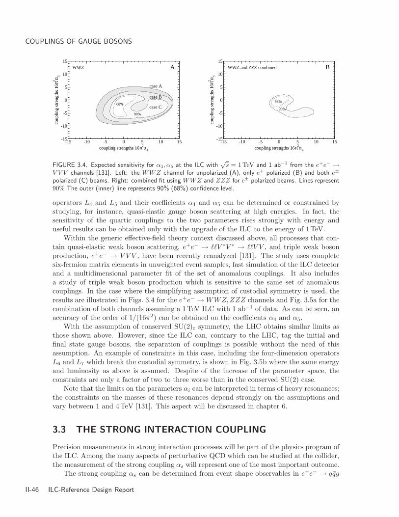
COUPLINGS OF GAUGE BOSONS
-15 -10 -5 0 5 10 15coupling strengths 16π2α
4
-15
-10
-5
0
5
10
15co
uplin
g st
reng
ths
16π2 α 5
WWZ
68%case C
A
case B
case A
90%
-15 -10 -5 0 5 10 15coupling strengths 16π2α
4
-15
-10
-5
0
5
10
15
coup
ling
stre
ngth
s 16
π2 α 5
WWZ and ZZZ combined
68%
B
90%
FIGURE 3.4. Expected sensitivity for α4, α5 at the ILC with√
s = 1 TeV and 1 ab−1 from the e+e− →V V V channels [131]. Left: the WWZ channel for unpolarized (A), only e+ polarized (B) and both e±
polarized (C) beams. Right: combined fit using WWZ and ZZZ for e± polarized beams. Lines represent90% The outer (inner) line represents 90% (68%) confidence level.
operators L4 and L5 and their coefficients α4 and α5 can be determined or constrained bystudying, for instance, quasi-elastic gauge boson scattering at high energies. In fact, thesensitivity of the quartic couplings to the two parameters rises strongly with energy anduseful results can be obtained only with the upgrade of the ILC to the energy of 1TeV.
Within the generic effective-field theory context discussed above, all processes that con-tain quasi-elastic weak boson scattering, e+e− → ``V ∗V ∗ → ``V V , and triple weak bosonproduction, e+e− → V V V , have been recently reanalyzed [131]. The study uses completesix-fermion matrix elements in unweighted event samples, fast simulation of the ILC detectorand a multidimensional parameter fit of the set of anomalous couplings. It also includesa study of triple weak boson production which is sensitive to the same set of anomalouscouplings. In the case where the simplifying assumption of custodial symmetry is used, theresults are illustrated in Figs. 3.4 for the e+e− → WWZ,ZZZ channels and Fig. 3.5a for thecombination of both channels assuming a 1TeV ILC with 1 ab−1 of data. As can be seen, anaccuracy of the order of 1/(16π2) can be obtained on the coefficients α4 and α5.
With the assumption of conserved SU(2)c symmetry, the LHC obtains similar limits asthose shown above. However, since the ILC can, contrary to the LHC, tag the initial andfinal state gauge bosons, the separation of couplings is possible without the need of thisassumption. An example of constraints in this case, including the four-dimension operatorsL6 and L7 which break the custodial symmetry, is shown in Fig. 3.5b where the same energyand luminosity as above is assumed. Despite of the increase of the parameter space, theconstraints are only a factor of two to three worse than in the conserved SU(2) case.
Note that the limits on the parameters αi can be interpreted in terms of heavy resonances;the constraints on the masses of these resonances depend strongly on the assumptions andvary between 1 and 4TeV [131]. This aspect will be discussed in chapter 6.
3.3 THE STRONG INTERACTION COUPLING
Precision measurements in strong interaction processes will be part of the physics program ofthe ILC. Among the many aspects of perturbative QCD which can be studied at the collider,the measurement of the strong coupling αs will represent one of the most important outcome.
The strong coupling αs can be determined from event shape observables in e+e− → qqg
II-46 ILC-Reference Design Report

The strong interaction coupling
16π2α5
16π2α4
16π2α5
16π2α4 16π
2α6
16π2α7
FIGURE 3.5. Limits of α4, α5 assuming SU(2)c conservation (a) and α4 - α7 without this assumption(b) from a combined analysis of three-vector-boson production and of vector-boson scattering assuming1000 fb−1 at
√s = 1 TeV. The dashed line represent 90% c.l. and the solid line 68%.
that are sensitive to the three-jet nature of the particle flow; examples of such observablesare the thrust, jet masses and jet rates. In this method, one usually forms a differentialdistribution, applies corrections for detector and hadronization effects and fits a perturbativeQCD prediction to the data, allowing αs to vary. Measurements from LEP and SLC haveshown that statistical errors below 0.001 can be obtained with samples of a few tens ofthousands hadronic events. With the current ILC design luminosities, hundreds of thousandsof e+e− → qq events can be produced each year and a statistical error on αs(MZ) below0.0005 can be achieved [132, 7]. The systematic error, however, is at present a factor tenlarger than this value and it is not clear, how much it can be improved by higher ordercalculations.
The GigaZ option also provides the possibility for a very accurate determination of thevalue of αs(MZ) via the measurement of the inclusive ratio of the Z boson decay widthsRhad = Γhad/Γ`. The current LEP data sample of 1.6 · 106 Z bosons provides an accuracy∆αs(MZ) = 0.0025 from the ratio Rhad [35]. At GigaZ, the statistical error can be lowered tothe level of 0.0004 but systematic errors arising from the hadronic and leptonic event selectionwill probably limit the precision to ∆αs(MZ) = 0.0008 [133]. This would be a very preciseand reliable measurement from a single and clean observable which is subject to very smalltheoretical uncertainties. Especially Rhad is unaffected by any non-perturbative corrections.
The translation of the measurements of αs(MZ) discussed above to other energies, αs(Q)with Q 6= MZ , requires the assumption that the running of the coupling is determined by theQCD β function. Since the logarithmic decrease of αs with energy is an essential component ofQCD, reflecting the underlying non-Abelian dynamics of the theory, it is important also to testthis energy dependence explicitly. Such a test would be particularly interesting if new coloredparticles were discovered, since deviations from QCD running would be expected at energiesabove the threshold for pair production of the new particles. Furthermore, extrapolation ofαs to very high energies of the order of MU = 1016 GeV can be combined with correspondingextrapolations of the weak and electromagnetic couplings in order to constrain the couplingunification or the GUT scale. Hence, it would be desirable to measure αs in the samedetector, with the same technique and by applying the same treatment to the data, at aseries of different energies Q, so as to maximize the lever-arm for constraining the running.This is shown in Fig. 3.6 where simulated measurements of αs(Q) at Q = 91, 500 and 800GeVare displayed, together with existing measurements in the range 20 ≤ Q ≤ 200GeV [132, 7].
It is therefore clear that ILC data adds significantly to the lever-arm in the energy evo-
ILC-Reference Design Report II-47

COUPLINGS OF GAUGE BOSONS
0
0.02
0.04
0.06
0.08
0.1
0.12
0.14
0.16
0.18
0.2
20 1050100
200
1000 50
0
1000
0
1000
00
1000
000
Deep Inelastic Scattering
Hadron Collisions
e+e− Annihilation
Linear e+e− Collider
Q [ GeV]
α S(Q
2 )
QCD αS(mZ2)=0.119
FIGURE 3.6. The evolution of αs with 1/ lnQ from various measurements; the data points are frompresent ones and the stars denote simulated ILC measurements for
√s = 91, 500 and 800 GeV.
lution of αs and allows a substantially improved extrapolation to the GUT scale. This isexemplified in Fig. 3.7 where the evolution of the three gauge couplings is displayed. Themeasurements at GigaZ will support unification at a scale MU ' 2 × 10¹⁶ GeV, with a pre-cision at the percent level. However, the couplings are not expected to meet exactly becauseof the high threshold effects at the scale MU . The quantitative evaluation of the discrepancywill provide important constraints on the particle content at the GUT scale.
102 106 1010 1014
Q [GeV]
0
10
20
30
40
50
601- 1
2- 1
3- 1
LHC &LC/GigaZ
1015 1016
Q [GeV]
24
25
FIGURE 3.7. Extrapolations of the gauge couplings as measured at ILC to the unification scale [134].
Many other aspects of QCD can be addressed at the ILC. In particular, the γγ and eγoptions offer a broad new area of QCD studies in two-photon interactions at high energy andluminosity. Examples are (see also chapter 4 for QCD studies in the process e+e− → tt) [7]the total cross section, the photon structure function and the annihilation of virtual photonsas a test of BFKL dynamics.
II-48 ILC-Reference Design Report

CHAPTER 4
Top quark physics
The top quark is the heaviest particle in the Standard Model and, thus, the most stronglycoupled to the electroweak symmetry breaking sector; it is therefore expected to play afundamental role in the dynamics behind the symmetry breaking mechanism. It might alsohold clues in solving the longstanding flavor problem and provide clear indications on newphysics beyond the Standard Model. For instance, if the Higgs mechanism should be verified,the measurement of the top quark Yukawa coupling would help to discriminate betweenSM and non–standard Higgs scenarios. If the new physics beyond the SM is sufficientlydecoupled, shifts in the production and decay properties of a SM–like top quark may be theonly evidence for it. With the precision ILC measurements, one could have sensitivity to newphysics at mass scales far above the electroweak symmetry breaking scale. For example, ithas been shown [124, 135] that in warped extra–dimensional models, as the top quark has awavefunction that is near the TeV brane, its production cross section at the ILC can revealKaluza–Klein excitations of gauge bosons with masses up to 10–100 TeV.
Precise and model–independent measurements at the ILC of the top couplings to weakgauge bosons will be sensitive to interesting sources of non–SM physics as many modelspredict anomalous top quark couplings. In Technicolor and other models with a strongly–coupled Higgs sector, non–standard CP–conserving couplings may be induced at the 5–10%level [136]. In supersymmetric and multi–Higgs models, CP–violating couplings may beinduced at the one-loop level, with predictions in the range 10−3–10−2 [137]. Little Higgs ortop–seesaw models predict definite shifts in the top quark couplings to the W and Z bosons.
High–precision measurements of the properties and interactions of the top quark aretherefore mandatory. The ILC will have broad capabilities to outline the top quark profilewith high precision and in a model–independent way. In particular, the tt threshold holdsthe promise of very precise measurements of the top quark mass and total decay width. Bothat threshold and in the continuum, the neutral and charged current interactions of the topquark can be very precisely determined. Its vector and axial–vector couplings to the Z bosonin the production vertex and to the W boson in the decay vertex, as well as its magnetic andelectric dipole moments, could be measured at the one percent level. The high luminosityexpected at the ILC will allow to determine the important top quark Yukawa coupling to theHiggs boson with a precision greatly exceeding that foreseen at the LHC.
Finally, if the threshold of new physics is nearby, new decay channels of the top quark,such as decays into a charged Higgs boson in supersymmetric or multi–Higgs doublet models,may be observed and studied in detail in the clean environment of the ILC.
ILC-Reference Design Report II-49

TOP QUARK PHYSICS
4.1 THE TOP QUARK MASS AND WIDTH
The top quark mass is a fundamental parameter of the SM and also a crucial ingredientof the electroweak precision measurement program, hence the importance to measure it asaccurately as possible [138]. In many extensions to the SM in which the Higgs boson mass canbe calculated, the theoretical prediction for M2
H depends sensitively on mt. For instance, inthe minimal supersymmetric extension of the SM, the radiative corrections grow as m4
t [41]. Inthis case, the expected LHC precision of 1 GeV on mt translates into a similar uncertainty forthe predicted value of the lighter Higgs boson mass Mh [41]. The anticipated accuracy at theILC is more than an order of magnitude better, obtaining a parametric error small enough toallow for a very incisive comparison of theory and measurement. A smaller uncertainty on mt
also improves the sensitivity to new physics causing anomalous W and Z couplings [139, 137].
Because of its large width, Γt ∼ 1.5 GeV, the top quark will decay before it hadronizes,thus non-perturbative effects are expected to be highly suppressed. As a result, the energydependence of the cross section σtt for e+e− → tt can be computed reliably, with an expectedincrease in rate by a factor of ten as the center-of-mass (CM) energy is varied by 5 GeVaround the threshold energy. The location of the rise of the cross section can be used toextract the value of mt, while the shape and normalization yield information about the totalwidth Γt, the strong coupling αs and eventually, the ttH Yukawa coupling gttH [140]. InRef. [141], three threshold observables: σtt, the peak of the top momentum distribution, andthe forward–backward charge asymmetry, were simultaneously fitted to obtain measurementuncertainties on mt, Γt, αs of 19 MeV, 32 MeV, and 0.0012, respectively. However thisstudy did not include a complete evaluation of important systematic uncertainties, such ase.g. the determination of the luminosity spectrum or theoretical uncertainties on differentialobservables. Figure 4.1 (left) demonstrates the sensitivity of the top mass measurementto these observables. It is expected that the top mass can be measured with a statisticaluncertainty of 40 MeV in a modest scan of 10 fb−1, a small fraction of a year at typicaldesign luminosities. A longer scan of about 100 fb−1 can determine the top width to 2%.
The threshold cross section has been calculated including some of the next-to-next-to-leading logarithmic (NNLL) QCD corrections, as shown in Fig. 4.1 (right) [142, 143]. Thefull NNLL contribution is not yet available, but the large size of the corrections relative to theNLL terms [144] suggests that the theoretical uncertainty on the cross section will ultimatelybe approximately δσtt/σtt ∼ ±3%, but the effect on the mass determination is small.
The high-precision measurements of the ILC at the tt threshold will determine a “thresh-old” (or resonance) mass parameter with an accuracy significantly below 100 MeV. Thisthreshold mass can then be translated into another short-distance mass that is useful as atheory input, such as the MS mass. This translation will give rise to an additional theoreticaluncertainty. The current estimate for the combined experimental and theoretical uncertaintyin the determination of the top-quark mass is about 100 MeV [145].
A threshold scan will require precise knowledge of the average c.m. energy and the shapeof the luminosity spectrum dL/dE [146]. Schemes for precision measurement of 〈Ecm〉 includethe use of beam spectrometers or using physics processes such as Z boson pair productionor radiative returns to the Z. The luminosity spectrum is determined by the beam spread,beamstrahlung and initial state radiation (ISR). All three effects will lead to a smearing ofthe tt threshold cross section, resulting in a significant reduction of the effective luminosityand hence the observed cross section, σobs(
√s) = L−1
0
∫ 10 L(x)σ(x
√s) dx.
The influence of the three effects is demonstrated in Fig. 4.2. The beam spread will
II-50 ILC-Reference Design Report
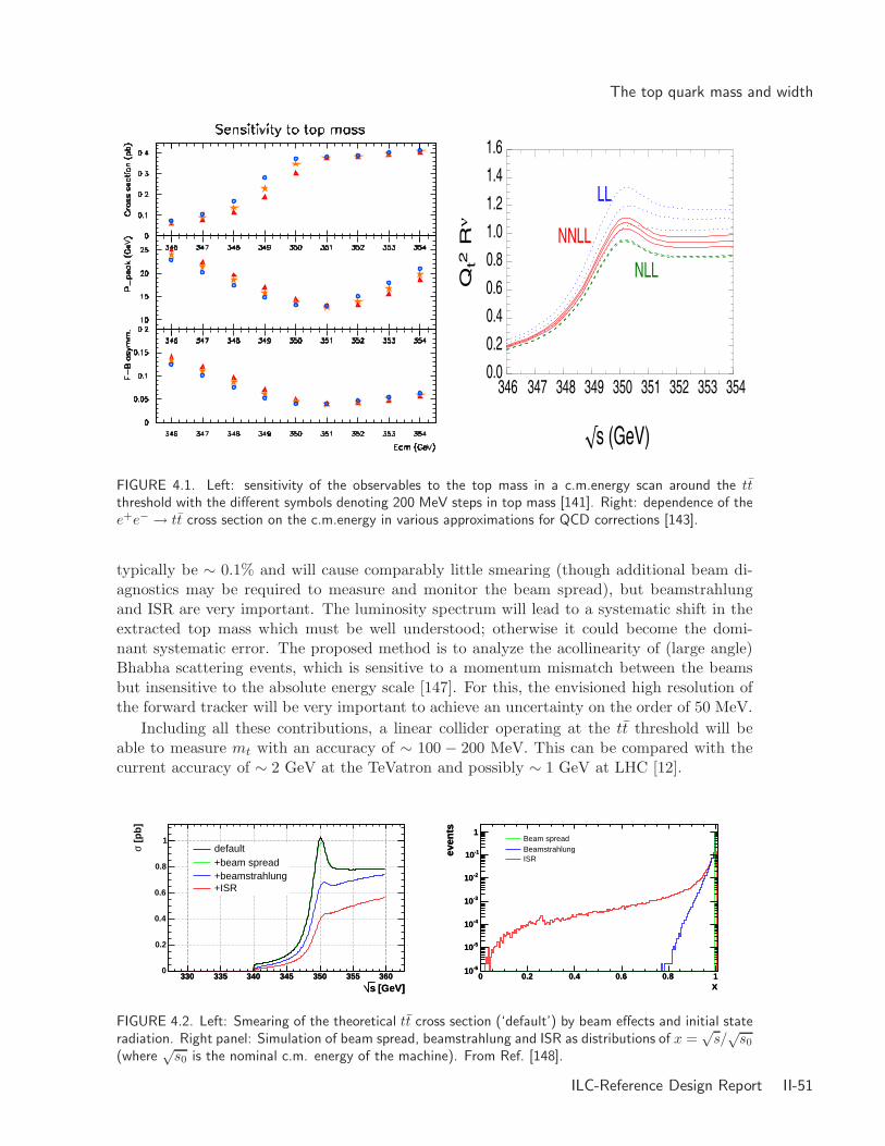
The top quark mass and width
FIGURE 4.1. Left: sensitivity of the observables to the top mass in a c.m.energy scan around the ttthreshold with the different symbols denoting 200 MeV steps in top mass [141]. Right: dependence of thee+e− → tt cross section on the c.m.energy in various approximations for QCD corrections [143].
typically be ∼ 0.1% and will cause comparably little smearing (though additional beam di-agnostics may be required to measure and monitor the beam spread), but beamstrahlungand ISR are very important. The luminosity spectrum will lead to a systematic shift in theextracted top mass which must be well understood; otherwise it could become the domi-nant systematic error. The proposed method is to analyze the acollinearity of (large angle)Bhabha scattering events, which is sensitive to a momentum mismatch between the beamsbut insensitive to the absolute energy scale [147]. For this, the envisioned high resolution ofthe forward tracker will be very important to achieve an uncertainty on the order of 50 MeV.
Including all these contributions, a linear collider operating at the tt threshold will beable to measure mt with an accuracy of ∼ 100 − 200 MeV. This can be compared with thecurrent accuracy of ∼ 2 GeV at the TeVatron and possibly ∼ 1 GeV at LHC [12].
[GeV]s330 335 340 345 350 355 360
[GeV]s330 335 340 345 350 355 360
[p
b]
σ
0
0.2
0.4
0.6
0.8
1default+beam spread+beamstrahlung+ISR
x0 0.2 0.4 0.6 0.8 1
even
ts
-610
-510
-410
-310
-210
-110
1
x0 0.2 0.4 0.6 0.8 1
even
ts
-610
-510
-410
-310
-210
-110
1Beam spreadBeamstrahlungISR
FIGURE 4.2. Left: Smearing of the theoretical tt cross section (‘default’) by beam effects and initial stateradiation. Right panel: Simulation of beam spread, beamstrahlung and ISR as distributions of x =
√s/√
s0
(where√
s0 is the nominal c.m. energy of the machine). From Ref. [148].
ILC-Reference Design Report II-51

TOP QUARK PHYSICS
4.2 TOP QUARK INTERACTIONS
4.2.1 The coupling to the Higgs boson
Near threshold, the tt pair interacts, in addition to the QCD potential, via a Yukawa potentialassociated with Higgs boson exchange. For a low Higgs boson mass, the tt cross sectionis a priori sensitive to the top-Higgs Yukawa coupling, gttH [141]. Even more sensitive isthe measurement of the e+e− → ttH cross section in the continuum, which is essentiallyproportional to g2
ttH as discussed in chapter 2.At the ILC with energies larger than 500 GeV, the process e+e− → ttH with the Higgs
decaying to W+W− or bb has the relatively clean signature of ≥ 6 jets in final state, with4 b–jets and multi–jet invariant mass constraints, but with backgrounds about three ordersof magnitude larger. The dominant backgrounds are radiative top production and/or decay(tt+jets) and irreducible ttZ(Z → bb) [149]. For Higgs bosons with 120–200 GeV masses,studies with events processed through a realistic detector simulation and involving rathersophisticated event selection procedures, have been performed [102, 101]. They demonstratethat one can measure gttH to 6–10% precision at
√s = 800 GeV with 1 ab−1 data [101].
However, even a 500 GeV ILC can significantly improve our knowledge of the the ttH Yukawacoupling and accuracies up to 10% can be achieved in the low Higgs mass range [102].
A recent reexamination of the LHC measurement of the coupling suggests it will bechallenging to reach this level of precision. However, when combined with ILC results at√
s = 500 GeV, LHC does better. ILC precision measurement of BR(H → W+W−) andBR(h → bb) replaces theory assumptions in the LHC measurements and leads to a bettercombined uncertainty of 10-15% or better for a large range of MH values [15, 67, 102].Therefore, for a number of years, the combination of results at the LHC and ILC (500 GeV)would yield the most precise determination of the top quark Yukawa coupling.
4.2.2 Couplings to electroweak gauge bosons
Since the charged electroweak current is involved in the top decay, tt production in e+e−
collisions is sensitive to both the neutral and charged gauge boson couplings of the topquark, and in the neutral case, directly sensitive to both the ttγ and ttZ vertices. Becausethe top quark width, Γt, is much larger than ΛQCD, the decay process is not influenced byfragmentation effects and decay products will provide useful information.
The most general tt(γ, Z) couplings can be written as [150, 151]
Γµtt(γ,Z)
= i e
γµ
[F γ,Z
1V + F γ,Z1A γ5
]+
( pt − pt)µ
2 mt
[F γ,Z
2V + F γ,Z2A γ5
], (i)
where the only form factors different from zero in the SM are
F γ1V =
2
3, FZ
1V =1
4 sin θW cos θW
(1 − 8
3sin2 θW
), FZ
1A = − 1
4 sin θW cos θW. (ii)
(e/mt) · F γ2A is the electric dipole moment form factor of the top quark and (e/mt) · FZ
2A the
weak electric dipole moment; (e/mt)·F γ,Z2V are the electric and weak magnetic dipole moments.
In the SM, the electric and dipole moment terms violate CP and receive contributions onlyat the three–loop level and beyond. The CP–conserving form factors are zero at tree–levelbut receive non–zero O(αs) QCD corrections.
II-52 ILC-Reference Design Report

Top quark interactions
TABLE 4.1The 1σ statistical uncertainties for the real parts of the (γ, Z)tt form factors obtained from an analysis
of the process e+e− → tt → `±+ jets for√
s = 500 GeV. Only one coupling at a time is varied.
Coupling LO SM Value P(e−)∫Ldt (fb−1) 1σ sensitivity
F γ1A 0 ±0.8 100 0.011
FZ1A −0.6 −0.8 100 0.013
F γ1V 2/3 ±0.8 200 0.047
FZ1V 0.2 ±0.8 200 0.012
F γ2A 0 +0.8 100 0.014
FZ2A 0 +0.8 100 0.052
F γ2V 0 ±0.8 200 0.038
FZ2V 0 ±0.8 200 0.009
In Table 4.1 is shown the 1σ sensitivity limits for the real parts of the tt(γ, Z) form factorsobtained from an analysis of the process e+e− → tt → `±+jets at
√s = 500 GeV [9]. Top
quarks are selected and reconstructed, and b quarks are tagged using a detector model withcombined efficiency of 20%, and purity of 88%. To extract limits on F γ,Z
1V and F γ,Z1A , the
angular distribution of the reconstructed top quark can be used. At the the ILC limits onF γ,Z
2A may be obtained from CP–violating angular asymmetries of the decay leptons, withoutassuming the tbW couplings to be vanishing [152]. Longitudinal e− beam polarization canbe used to enhance the sensitivity, as well as to obtain independent limits on F γ
2A and FZ2A,
when both are simultaneously kept nonzero. Combinations of decay lepton energy and angularasymmetries can be made sensitive to anomalous couplings either in the production or thedecay by a suitable choice of cuts on the lepton energy [153].
F γ,Z1V and F γ,Z
2V are derived from the left–right polarization asymmetry ALR and F γ,Z2A
from the angular distribution of the reconstructed top quark and the decay angles of the tand t. The limits shown in Table 4.1 could be strengthened with positron beam polarization,mostly from the increased tt cross section: with Pe+ = 0.5, σ(tt) is about a factor 1.45 larger,improving the precision in the measurement of ALR by nearly a factor of 3 [17]. Increasingthe c.m. energy to
√s = 800 GeV improves the limits by a factor 1.3–1.5 [154].
The most general tbW couplings can be parameterized in the form [151]
ΓµtbW = − g√2
Vtb
γµ
[fL1 PL + fR1 PR
]− i σµν
MW
(pt − pb)ν[fL2 PL + fR2 PR
], (iii)
where PR,L= 12(1±γ5). In the limit mb → 0, fR1 and fL2 vanish and, in the SM, fL1 = 1 and
all other form factors are zero at tree–level. The tbW vertex can be parameterized similarly.The fR2 coupling, corresponding to a V+A tbW interaction, can be measured in tt decays
with a precision of about 0.01 for√
s = 500 GeV and 500 fb−1 if electron and positron beampolarization are available [151]. This quantity can also be measured at the LHC, but theexpected limit is a factor three to eight weaker [155].
The ILC can measure the tbW interaction to significant precision by studying tt produc-tion below threshold [156]. At c.m. energies below 2mt but still above mt, the total rate fore+e− → W+W−bb is dominated by contributions from the virtual tt diagrams in a kinematicconfiguration where one top is on-shell and the other is off-shell. Other contributions include
ILC-Reference Design Report II-53

TOP QUARK PHYSICS
single top quark production and, to a smaller extent, non-resonant interfering backgrounds.The rate becomes very sensitive to the tbW interaction, essentially because the narrow widthapproximation is no longer valid when the top momentum is off-shell.
For simplicity, the analysis focuses on the case of all couplings but fL1 equal to zero anddefines the effective V–A coupling as gtbW = gVtbf
L1 . Only the semi-leptonic six-body final
state where one W boson decays to a pair of jets and the other into an readily tagged lepton(e, µ or τ), is considered. Combining the below-threshold cross section measurement withthe Γt extracted from the threshold scan permits extraction of gtbW and Γt independently.Under the assumption that the width is measured to an accuracy of 100 MeV, gtbW can bemeasured to the 3% level, which would represent better than a factor of two improvementcompared to the LHC.
Figure 4.3 shows the expected bounds on the SM–like top axial ttZ and left–handedtbW interactions and the discriminating power the bounds can place on new physics models.Included in the plot are the 1σ constraints on the independently varied axial ttZ couplingfrom the LHC and ILC [9], and the direct constraints on the left-handed tbW coupling fromthe LHC [155]. Predicted deviations from a few representative models are also superimposed:a Little Higgs model with T-parity, a model of top-flavor, and a model with a sequential fourthgeneration whose quarks mix substantially with the third family. The little Higgs model withT–parity has a heavy top quark partner T with a mass assumed to be mT = 500 GeV (thenumbers on the plot indicate the strength of the hT t interaction); the top–flavor model hasa mixing angle sin φ = 0.9 (numbers indicate the mass of the heavy Z ′). Top–seesaw modelsgenerate the same mixing effect as the little Higgs models and, thus, trace out the same linein the plane of deviations in the ttZ and tbW as the seesaw model parameters are varied.
-0.2 -0.1 0 0.1 0.2∆gLgL HW t bL
-0.2
-0.1
0
0.1
0.2
∆g Ag
AHZ
ttL
LHC
ILC4th Gen.
T-Parity
.5
1
1.5
TopFlavor700
1.0
FIGURE 4.3. Expected bounds on axial ttZ and left–handed tbW couplings from direct LHC (olive) andILC (red) measurements; superimposed are predicted deviations from representative models [156].
Finally, the ILC has excellent reach for the measurement of the tensor coupling tZq;see for instance Ref. [157]. At the ILC, both the anomalous production e+e− → tq anddecay e+e− → tt, t → V q mechanisms can be explored, permitting sensitivity to flavorchanging neutral current interactions. With 45% positron and 80% electron polarization at√
s = 500 GeV, 100 fb−1 of data would result e.g. in a sensitivity to BR(t → γq) of 2× 10⁻⁵.The search sensitivity might be significantly increased if the ILC runs in the γγ mode [158].
II-54 ILC-Reference Design Report

New decay modes
4.2.3 Couplings to gluons
The ILC can be competitive with and complementary to the LHC in the measurement of thestrong top quark coupling to gluons and would allow more refined tests of perturbative QCD[7]. Hard gluon radiation in tt events [159] would allow several tests of the strong dynamicsof the top quark: test of the flavour–independence of strong interactions, limits on anomalouschromo-electric and/or chromo-magnetic dipole moments [160] and the determination of therunning top quark mass. In turn, soft gluon radiation in tt events is expected to be stronglyregulated by the large top mass and width and would provide additional constraints onthe total decay width Γt [161]. Color reconnection and Bose-Einstein correlations are alsoimportant to study precisely [162] as they may affect the precision with which the top quarkmass can be reconstructed kinematically via their multijet decays.
Furthermore, polarized electron and positron beams can be exploited to test symmetriesusing multi–jet final states. For polarized e+e− annihilation to three hadronic jets, one candefine the triple product Se · (k1 × k2), which correlates the e− beam polarization vector Sewith the normal to the three–jet plane defined by k1 and k2, the momenta of the two quarkjets. If the jets are ordered by momentum (flavour), the triple–product is CP–even (odd)and T–odd [163]. In the SM, the contributions to the T–odd form are expected to be verysmall and limits have been set for the bbg system. At the ILC, these observables will providean additional possibility to search for anomalous effects in the ttg system.
4.3 NEW DECAY MODES
Besides the standard channel t → bW , new decays of the top quark can occur in some exten-sions of the SM. The prominent example is the top quark decay into a charged Higgs boson,t → bH+, in supersymmetric extensions of the SM or in multi–Higgs doublet extensions. Thischannel has been mentioned in chapter 2 in the context of the MSSM and in this case, thecoupling of the H± bosons to top and bottom quarks is a mixture of scalar and pseudoscalarcurrents and depend only on the ratio of the vev’s of the two Higgs doublet fields tan β,
gH−tb ∼ mb tan β(1 + γ5) + mtcotβ(1 − γ5) (iv)
The coupling is therefore very strong for small or large tan β values for which the mt
component is not suppressed or the mb component is strongly enhanced. The branchingratio BR(t → bH+) = Γ(t → bH+)/[Γ(t → bW ) + Γ(t → bH+)] is displayed in the left–handside of Fig. 4.4 as a function of MH+ for two values tan β = 3 and 30. As can been seen, itis rather substantial being still at the per–mille level for H+ masses as large as 150 GeV.
Since the cross section for top quark pair production is of the order of σ(e+e− → tt) ∼ 0.5pb at a
√s = 500 GeV ILC, the cross section times the branching ratio for the production
of one charged Higgs boson is rather large if MH± is not too close to mt for the decay notto be suppressed by the small phase space. This is shown in the right–hand side of Fig. 4.4where on can see that, for MH± <∼ 150 GeV, the rates are of the same order of magnitude asthe ones from direct pair production, e+e− → H+H−, which is displayed for comparison.
In the MH± range under consideration, the main two–body decays of the charged Higgsboson will be into τντ and cs pairs with the former being largely dominating for the chosentan β values; see Fig. 2.17. This results in a surplus of τ final states over e, µ final states,an apparent breaking of lepton universality. For low values of tan β, the three–body decay
ILC-Reference Design Report II-55

TOP QUARK PHYSICS
modes H± → hW ∗, AW ∗ → bbW will lead to multi b and W final states. These signals willbe rather easy to be disentangled from the backgrounds in the clean ILC environment.
tan = 330BR(t! H+b)
MH 1701601501401301201101009080
0.10.010.001 tan = 30tan = 3t;t! H e+e ! H+H
ps = 500 GeV(e+e ! H +X) [fb]
MH [GeV] 250200160130
3001001010.3
FIGURE 4.4. Left: the branching ratio for the decay t → H+b as a function of MH+ for tan β = 3 and30 in the MSSM. Right: the cross sections times branching ratio for the production of one charged Higgsboson from top decays, e+e−tt and t → H+b, at the ILC with
√s = 500 GeV; the direct e+e− → H+H−
cross section is shown for comparison. From Ref. [40].
This signal will be first observed at the LHC as it is one of the main discovery channelsfor charged Higgs bosons. However, the ILC will provide a very important information: theprecise measurement of the t → H+b branching ratio would allow to determine the parametertan β which is known to be rather difficult to access otherwise; see chapter 5.
In supersymmetric models, another possible and interesting decay mode of the top quarkwould be into its scalar partner t1 and the lightest neutralino χ0
1 which is supposed to formthe dark matter in the universe, t → t1χ
01. In the minimal supersymmetric extension with
universal masses for the superpartners of the gauge bosons at the high GUT scale, the phasespace for this decay is squeezed by the constraints on the t1 and χ0
1 masses from LEP andthe Tevatron. In non minimal extensions, the decay might be kinematically allowed and, inthis case, branching ratios of the order of a few percent would be possible. Since the maindecay modes of the top squark in this mass range are the loop induced t1 → cχ1
0 and thefour–body t1 → bf fχ1
0 channels, the signal will consist on the missing energy due to theescaping neutralinos. While it is overwhelmed by huge QCD backgrounds at the LHC, thissignature should be easy to detect at the ILC.
Finally, flavor changing neutral current (FCNC) decays of the to quark may be also ob-served. If new quark species exist and do not belong to the standard doublet/singlet assign-ments of isospin multiplets, they will mix with the top quark, breaking the GIM mechanism
and allowing for FCNC top–charm couplings of order√
mtmc/M2X to be induced. In this
case, besides breaking the universality of the V − A chiral Wtb current, FCNC top quarkdecays such as t → cγ or t → cZ may occur at the level of a few permille and can be detectedat the ILC [164]. However, the large number of top quarks produced at the LHC allows tosearch for these rare FCNC decays down to branchings ratio less than 10−4.
II-56 ILC-Reference Design Report

CHAPTER 5
Supersymmetry
5.1 INTRODUCTION
5.1.1 Motivations for supersymmetry
Despite its enormous success in describing almost all known experimental data availabletoday, the Standard Model (SM) is widely believed to be an effective theory valid only atthe presently accessible energies. Besides the fact that it does not say anything about thefourth fundamental force of nature, the gravitational force, and does not explain the patternof fermion masses, it has at least three severe problems which call for new physics. Giventhe high–precision data and the particle content of the SM, the energy evolution of the gaugecoupling constants is such that they fail to meet at a common point, the grand unification(GUT) scale. Moreover, the SM does not include any candidate for a particle that is absolutelystable, fairly massive, electrically neutral and having only weak interactions, which accountsfor the cold dark matter (DM) that makes up ≈ 25% of the present energy of the universe.Finally, in the SM, the radiative corrections to the Higgs boson mass squared are quadraticallydivergent and MH , which is expected to lie in the range of the electroweak symmetry breakingscale, O(100) GeV, prefers to be close to the cut–off scale beyond which the theory ceases tobe valid, the very high GUT or Planck scales.
Supersymmetry (SUSY) [165], which predicts the existence of a partner to every knownparticle that differs in spin by 1
2 , is widely considered as the most attractive extension of theSM. Firstly, SUSY has many theoretical virtues [166]: it is the first non–trivial extensionof the Poincare group in quantum field theory which, when made local, necessarily includesEinsteins’s theory of gravity, and it appears naturally in superstring theories. These featuresmay help to reach the ultimate goal of particle physics: the unification of all forces includ-ing gravity. However, the most compelling arguments for SUSY are phenomenological ones:when it is realized at low energies, it can solve at once all the above three problems of theSM. Indeed, the main reason for introducing low energy supersymmetric theories in particlephysics is their ability to solve naturally the fine–tuning problem [167]: SUSY prevents MH
from acquiring very large radiative corrections as the quadratic divergent loop contributionsof the SM particles are exactly canceled by the corresponding loop contributions of their su-persymmetric partners. In fact, SUSY allows one to understand the origin of the electroweaksymmetry breaking itself in terms of radiative corrections triggered by SUSY breaking [168],which must occur as the newly predicted superparticles have not been observed up to now
ILC-Reference Design Report II-57

SUPERSYMMETRY
and must be thus heavy. In addition, the new SUSY particle spectrum contributes to theevolution of the three gauge couplings and allows their unification at a scale MGUT ' 2·1016
GeV [169]. Finally, a discrete symmetry called R–parity [170] can be naturally present withthe major consequence that the lightest supersymmetric particle (LSP) is absolutely stable; inmany cases, this particle has the right properties and the required cosmological relic densityto account for the cold DM [171, 172].
5.1.2 Summary of SUSY models
The most economical low–energy globally supersymmetric extension of the SM is the minimalsupersymmetric Standard Model (MSSM) [173]. In this model, one assumes the minimal (SM)gauge group, the minimal particle content [i.e., three generations of fermions and their spin–zero partners as well as two Higgs doublet superfields to break the electroweak symmetry ina consistent manner], and R–parity conservation, which makes the LSP absolutely stable. Inorder to explicitly break SUSY, a collection of soft terms is added to the Lagrangian: massterms for the gauginos, the SUSY spin–1
2 partners of the gauge bosons, mass terms for thesfermions, the spin–0 partners of the SM fermions, mass and bilinear terms for the two Higgsfields and trilinear couplings between sfermion and Higgs fields.
In the most general case, the soft SUSY–breaking terms will introduce a huge numberof unknown parameters, O(100). However, in the absence of complex phases and intergen-erational sfermion mixing and if the universality of the two first generations of sfermionsis assumed, to cope in a simple way with the severe experimental constraints, this num-ber reduces to O(20). Furthermore, if the soft SUSY–breaking parameters obey a set ofboundary conditions at a high energy scale, all potential phenomenological problems of thegeneral MSSM can be solved with the bonus that, only a handful of new free parameters arepresent. The underlying assumption is that SUSY–breaking occurs in a hidden sector whichcommunicates with the visible sector only “flavor–blind” interactions, leading to universalsoft breaking terms. This is assumed to be the case in the celebrated minimal supergravity(mSUGRA) model [174] or constrained MSSM (cMSSM) which is often used as a benchmarkscenario in phenomenological analyses.
Besides the GUT scale which is derived from the unification of the three gauge couplingconstants, the cMSSM has only four free parameters plus a sign:
m0, m1/2, A0, tan β, sign(µ) ,
where m0,m1/2 and A0 are, respectively, the common soft terms of all scalar (sfermion andHiggs) masses, gaugino (bino, wino and gluino) masses and trilinear scalar interactions, alldefined at the GUT scale. tan β is the ratio of the vacuum expectation values (vev’s) of thetwo Higgs doublets at the weak scale and µ is the supersymmetric Higgs(ino) mass parameter.As in the MSSM in general, all soft SUSY–breaking parameters at the weak scale are thenobtained via known Renormalization Group Equations (RGEs). The masses of the physicalstates, the spin–1
2 charginos χ±1,2 and neutralinos χ0
1,2,3,4 which are mixtures of the SUSY
partners of the gauge and Higgs bosons, the two scalar partners f1,2 of the SM fermions andthe five MSSM Higgs bosons h,H,A and H± are then obtained by diagonalyzing the relevantmass matrices. In this scenario, the LSP is in general the lightest neutralino χ0
1.
There are also other constrained MSSM scenarios with only a few basic input parameters,two of them being the anomaly (AMSB) [175] and gauge (GMSB) [176] mediated models inwhich SUSY–breaking also occurs in a hidden sector but is transmitted to the visible one by
II-58 ILC-Reference Design Report

Introduction
anomalies or by the SM gauge interactions; in the later case, a very light gravitino is the LSP1.On the other hand, one can slightly depart from the restrictive minimality of the MSSM andinteresting examples are the CP violating MSSM [43] where some SUSY parameters can becomplex, the NMSSM [49] in which the spectrum is extended to include a singlet superfieldand R–parity violating models [178] in which the LSP is not stable.
The Terascale is a mystery that will be revealed by the LHC and the ILC and bothmachines will have an important role to play in deciphering it. In particular the high precisionof the ILC will be necessary to understand the new physics, no matter which scenario naturehas chosen. In this chapter, we will mainly focus on the unconstrained and constrainedMSSMs defined above as they are very well defined and have been studied in great detail.These models provide us with an excellent testground for the opportunities offered by thehigh–energy colliders, the ILC in particular, in reaching out to new physics domains.
5.1.3 Probing SUSY and the role of the ILC
To prove and to probe supersymmetry, one not only needs to produce the new particles butalso, and this is equally important, to verify its most fundamental predictions in a modelindependent way. A detailed investigation of the properties of the SUSY and Higgs particlespectrum is thus required and, in particular, one needs to:
• measure the masses and mixings of the newly produced particles, their decay widthsand branching ratios, their production cross sections, etc...;
• verify that there are indeed the superpartners of the SM particles and, thus, determinetheir spin and parity, gauge quantum numbers and their couplings;
• reconstruct the low–energy soft–SUSY breaking parameters with the smallest numberof assumptions, that is, in as model independent way as possible;
• ultimately, unravel the fundamental SUSY breaking mechanism and shed light on thephysics at the very high energy (GUT, Planck?) scale.
Furthermore, the very precise knowledge of the properties of the lightest SUSY particleand its interactions with the standard and other SUSY particles is mandatory to predictthe cosmological relic density of the DM, as well as its rates in direct and indirect detectionastroparticle experiments. Achieving this goal would be the decisive test that a particularphysics scenario is the solution of the DM puzzle and would lay an additional bridge betweencollider physics and the physics of the early universe.
In most areas of the MSSM parameter space, in particular in cMSSM type scenarios(except in the focus point scenario to be discussed later in chapter 7), the colored squarksand gluinos turn out to be much heavier than the non–colored sparticles, the sleptons aswell as the charginos and neutralinos; see Fig. 5.1. If the masses of the former sparticles dotnot significantly exceed the TeV scale, as required from naturalness arguments, they can becopiously produced at the LHC either in pairs or in association [12, 13]. They will then decayin potentially long chains which end in the LSP neutralino that signals its presence only viamissing energy. These decay chains will involve the other neutralinos and the charginos, andpossibly the sleptons, so that one can have access to these weakly interacting particles aswell. Typically, one faces a situation in which several SUSY particles are present in the sameevent, leading to rather complicated final state topologies which are subject to very large
1In fact, in mSUGRA–like models, one can also have the gravitino being the LSP in large areas of theparameter space [177]; this issue will be discussed in the cosmology chapter.
ILC-Reference Design Report II-59

SUPERSYMMETRY
backgrounds from the SM and, more importantly, from SUSY itself. At the LHC, sparticlemass differences can be determined by measuring the endpoints or edges of invariant massspectra (with some assumptions on particle identification within the chains) and this resultsin a strong correlation between the extracted masses; in particular, the LSP mass can beconstrained only weakly [15]. Therefore, only in specific constrained scenarios with a handfulof input parameters, that some elements of SUSY can be reconstructed in the complicatedenvironment of the LHC.
0
100
200
300
400
500
600
700
m [GeV]SPS1a′ mass spectrum
lR
lLνl
τ1
τ2ντ
χ01
χ02
χ03
χ04
χ±
1
χ±
2
qR
qL
g
t1
t2
b1
b2
h0
H0, A0 H±
200 350 500 1000
100000
10000
1000
100
10
1
0.1
HZ
ZZ
WW
tt
ff (e e ) [fb]σ + -
s[GeV]
χ χ 1 1+ -
t1t1
χ χ 1 20 0
µ µ1 1+ -
FIGURE 5.1. The spectrum of SUSY and Higgs particles in the benchmark SPS1a′ cMSSM point [179](left) and the production cross sections for various SM and SUSY processes in e+e− collisions as a functionof the c.m. energy in this scenario (right).
On the other hand, the non–colored SUSY particles (and certainly the lightest Higgsboson) would be accessible at the ILC with a c.m. energy of
√s = 500 GeV, to be eventually
upgraded to 1 TeV. This is, for instance the case in a cMSSM typical scenario called SPS1a′
[179] as shown in Fig. 5.1. The cross sections for chargino, neutralino and slepton pairproduction, when the states are kinematically accessible, are at the level of 10–100 fb, whichis only a few orders of magnitude below the dominant SM background processes; Fig. 5.1.Given the expected high–luminosity and the very clean environment of the machine, largesamples of events will be available for physics analyses [7, 180]. At the ILC, it will be thuseasy to directly observe and clearly identify the new states which appeared only throughcascade decays at the LHC. Most importantly, thanks to the unique features of the ILC,tunable energy which allows threshold scans, the availability of beam polarization to selectgiven physics channels and additional collider options such as e−e− which allow for newprocesses, very thorough tests of SUSY can be performed: masses and cross sections can bemeasured precisely and couplings, mixing angles and quantum numbers can be determinedunambiguously. Furthermore, the ILC will provide crucial information which can be used asadditional input for the LHC analyses, as would be e.g. the case with the LSP mass. Thecoherent analyses of data obtained at the LHC and the ILC would allow for a better andmodel independent reconstruction of the low energy SUSY parameters, connect weak–scaleSUSY with the more fundamental underlying physics at the GUT scale, and provide thenecessary input to predict the LSP relic density and the connection with cosmology.
II-60 ILC-Reference Design Report

Precision SUSY measurements at the ILC
To highlight the unique abilities of the ILC to address these issues, we will often use forillustration the cMSSM benchmark SPS1a′ point with basic inputs [179]:
m1/2 =250 GeV, m0 =70 GeV, A0 =−300 GeV, tan β=10 and µ > 0,which, using one of the RGE codes (SPHENO) of Ref. [181], leads to the SUSY spectrum ofTab. 5.1. This testcase point is close to the point SPS1a [182] with m0 = −A0 = 100 GeV andthe same m1/2, tan β and µ values, which has been used for detailed LHC [183, 184] as wellas ILC analyses, but is not compatible anymore with all collider or cosmological constraints.
TABLE 5.1Some superparticle and their masses (in GeV) for the cMSSM SPS1a′ and SPS1a reference points.
p/mass χ01 χ0
2 χ±1 e1/µ1 e2/µ2 νe/νµ τ1 τ2 ντ t1 b1
SPS1a′ 97.7 183.9 183.7 125.3 189.9 172.5 107.9 194.9 170.5 366.5 506.3
SPS1a 96.1 176.8 176.4 143.0 202.1 186.0 133.2 206.1 185.1 379.1 491.9
5.2 PRECISION SUSY MEASUREMENTS AT THE ILC
5.2.1 The chargino/neutralino sector
The two charginos χ±1,2 and the four neutralinos χ0
1,2,3,4 are obtained by diagonalyzing themass matrices of the charged and neutral gauginos and higgsinos. For charginos, the matrixdepends on the wino and higgsino mass parameters M2 and µ and on tan β; for neutralinos,the bino mass parameter M1 enters in addition. These parameters determine to a large extentthe production and decay properties of the χ0
i , χ±i states that we will call “inos” for short.
Charginos are produced in pairs, e+e− → χ+i χ−
j , through s–channel γ/Z boson and t–
channel sneutrino exchanges; the latter contribution can be suppressed with polarized e−R/e+L
beams. Neutralino pair production, e+e− → χ0iχ
0j , proceeds through s–channel Z boson and
t– and u–channel eL,R exchanges. The ino states decay into lighter charginos and neutralinosand (possibly virtual) gauge or Higgs bosons as well as sfermion–fermion pairs; for the lighterinos, one would then have the topologies χ±
1 → f f ′χ01 and χ0
2 → f fχ01. These final states can
be easily detected as the production cross sections are sizable and the backgrounds involvinga large amount of missing energy are small.
The chargino masses can be determined in the continuum from the di–jet energy dis-tributions in the process e+e− → χ+
1 χ−1 → `±νqq′χ0
1χ01, which leads to a mass resolution
∆mχ±
1/mχ0
1at the permille level. This can serve to optimize a scan around threshold which,
because of the steep σ ∝ βχ rise of the excitation curve with the velocity, would lead to a massresolution ∆mχ±
1=O(50) MeV for mχ±
1∼170 GeV; Fig. 5.2. The di–jet mass spectrum in χ±
1
decays allows also to determine the chargino–neutralino mass difference with a high preci-sion, ∆(mχ±
1−mχ0
1)=O(50) MeV, from which one can infer the mass of the escaping lightest
neutralino. If the chargino happens to be almost degenerate with the LSP neutralino, as istypically the case in AMSB models, one can use ISR photons in the process e+e− → χ+
1 χ−1 γ
to measure both the χ±1 and χ±
1 − χ01 masses from the spectra of, respectively, the photon
recoil mass which peaks at 2mχ±
1and the energy of the soft pions from χ+
1 → χ01 +πsoft which
peaks at ∆mχ±
1−mχ0
1; Fig. 5.2. An uncertainty of a few percent is obtained in both cases.
ILC-Reference Design Report II-61

SUPERSYMMETRY
300 350 400 450 500M [GeV]rec
0
0.5
1
1.5
2
E [
GeV
]
plo
ns/
0.0
5 G
eV
with beamstrahlung
M = 172.0 GeV
FIGURE 5.2. The cross section for e+Re−L → χ+
1 χ−1 → `±ν`χ
01qq
′χ01 near threshold, with the error bars
obtained with a luminosity of 10 fb−1 per point [185] (left). The initial state radiated photon recoil massfor the process e+
Re−L → χ+1 χ−
1 γ → π+π−γ /E (right) [186].
Similarly to the chargino case, the di–lepton mass and energy spectra in the processe+e− → χ0
2χ01 → `+`−χ0
1χ01, allow to determine the mass difference of the two neutralinos
at the permille level. In the case where the neutralino χ02 decays dominantly via a real or
virtual stau lepton, χ02 → τ1τ → τ+τ−χ0
1, which might occur at high tan β values that leadto light tau sleptons, the resolution on the χ0
2 mass deteriorates to the level of a few percent.The reason is that the energy of the τ ’s cannot be reconstructed because of the missingneutrinos and, in fact, this is also the case for charginos in the decays χ±
1 → τ±1 ντ → τ±ντχ
01.
A better mass resolution, O(100) MeV, can be obtained with a threshold scan in scenarioswhere sleptons are light, even in topologies involving τ ’s. For very heavy selectrons the erroris larger since only the s–channel Z exchange contribution is present, leading to relativelysmaller cross sections and a less steep excitation curve, σ ∝ β3
χ because of the Majorananature of the neutralinos. An exception is when the neutralinos that are produced in mixedpairs have opposite CP parities, in which case the cross section increases steeply in S–waves.
Note that for the verification of the spin–12 character of the neutralinos and charginos,
neither the onset of the excitation curves near threshold nor the angular distributions inthe production processes provide unique signals of the spin [187]. However, decay angulardistributions of polarized neutralinos/charginos that are pair produced with polarized beamsprovide an unambiguous determination of the spin–1
2 character of the particles albeit at theexpense of more involved experimental analyses [187].
The e+e− → χ+i χ−
j production cross sections are binomials in the chargino mixing anglescos 2φL,R and the latter can be determined in a model independent way using polarizedbeams. This is exemplified in the contours shown in Fig. 5.3 for two c.m. energies andassuming Pe− = 0.8 and Pe+ = 0.5. At
√s = 500 GeV, two regions of the plane are selected,
but one of them can be removed by moving to lower c.m. energies. For SPS1a, includingthe uncertainties in the mass measurements, one obtains the 95% CL limited range for themixing angles cos 2φL = [0.62, 0.72] and cos 2φR = [0.87, 0.91]. In the CP conserving MSSM,the information obtained from chargino production and decay processes would be sufficient todetermine the basic parameters entering the χ±–χ0 system with a very good accuracy. Also,we recall that the t–channel ν exchange can be suppressed using polarized beams and mνe
II-62 ILC-Reference Design Report
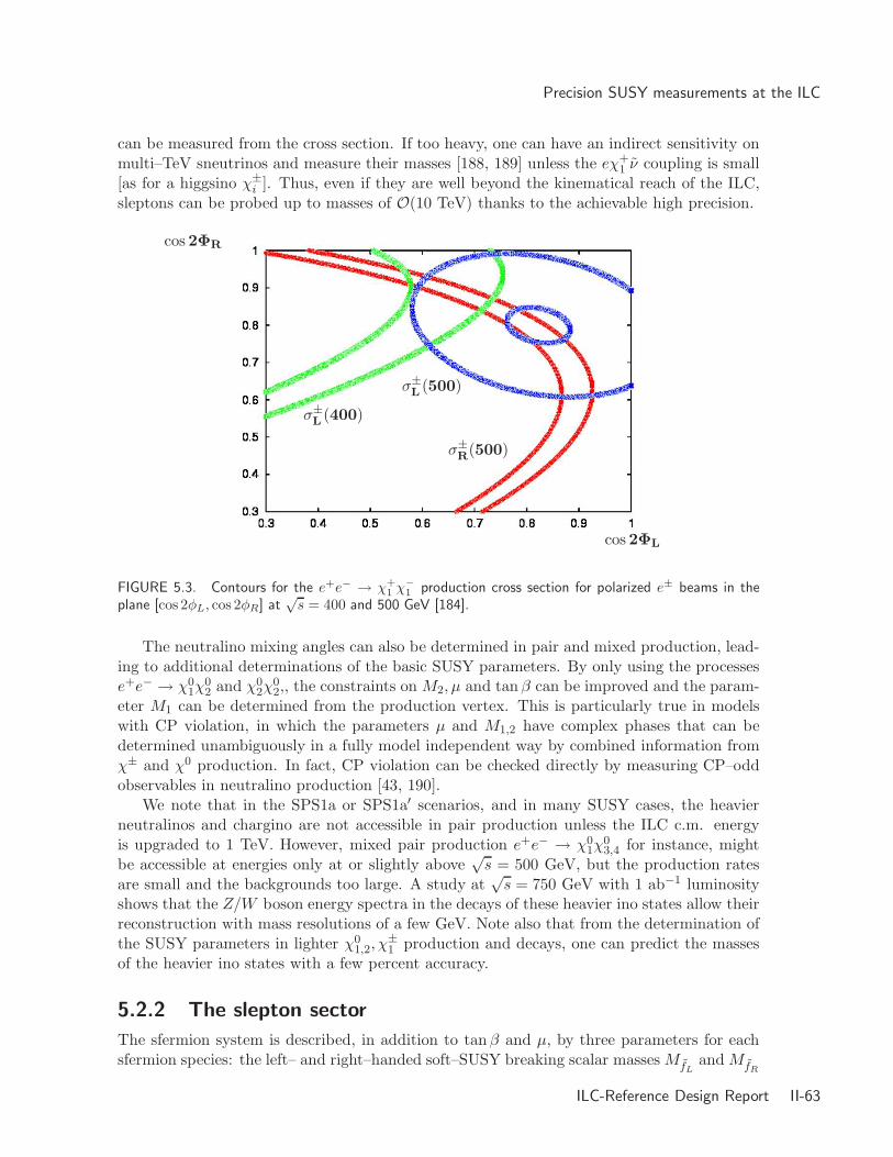
Precision SUSY measurements at the ILC
can be measured from the cross section. If too heavy, one can have an indirect sensitivity onmulti–TeV sneutrinos and measure their masses [188, 189] unless the eχ+
1 ν coupling is small[as for a higgsino χ±
i ]. Thus, even if they are well beyond the kinematical reach of the ILC,sleptons can be probed up to masses of O(10 TeV) thanks to the achievable high precision.
cos 2ΦL
cos 2ΦR
σ±L
(500)
σ±L
(400)
σ±R
(500)
FIGURE 5.3. Contours for the e+e− → χ+1 χ−
1 production cross section for polarized e± beams in theplane [cos 2φL, cos 2φR] at
√s = 400 and 500 GeV [184].
The neutralino mixing angles can also be determined in pair and mixed production, lead-ing to additional determinations of the basic SUSY parameters. By only using the processese+e− → χ0
1χ02 and χ0
2χ02,, the constraints on M2, µ and tan β can be improved and the param-
eter M1 can be determined from the production vertex. This is particularly true in modelswith CP violation, in which the parameters µ and M1,2 have complex phases that can bedetermined unambiguously in a fully model independent way by combined information fromχ± and χ0 production. In fact, CP violation can be checked directly by measuring CP–oddobservables in neutralino production [43, 190].
We note that in the SPS1a or SPS1a′ scenarios, and in many SUSY cases, the heavierneutralinos and chargino are not accessible in pair production unless the ILC c.m. energyis upgraded to 1 TeV. However, mixed pair production e+e− → χ0
1χ03,4 for instance, might
be accessible at energies only at or slightly above√
s = 500 GeV, but the production ratesare small and the backgrounds too large. A study at
√s = 750 GeV with 1 ab−1 luminosity
shows that the Z/W boson energy spectra in the decays of these heavier ino states allow theirreconstruction with mass resolutions of a few GeV. Note also that from the determination ofthe SUSY parameters in lighter χ0
1,2, χ±1 production and decays, one can predict the masses
of the heavier ino states with a few percent accuracy.
5.2.2 The slepton sector
The sfermion system is described, in addition to tan β and µ, by three parameters for eachsfermion species: the left– and right–handed soft–SUSY breaking scalar masses MfL
and MfR
ILC-Reference Design Report II-63

SUPERSYMMETRY
and the trilinear couplings Af . Sfermion mixing turns the current eigenstates fL and fR intothe mass eigenstates f1 and f2, but only in the case of the third generation that this mixing,∝ mf , is important [for the first two sfermion generations, since mf → 0, universality canbe assumed in general as will be done here]. In the case of τs, it is significant at large tan β,leading to a τ1 that is much lighter than the other sleptons.
The production of the second and third generation sleptons in e+e− collisions is mediatedby s–channel γ/Z exchanges in P–waves with a characteristic rise of the excitation curve,σ ∝ β3
˜. The production of selectrons and electronic sneutrinos proceeds, in addition, through
t–channel exchanges of neutralinos or charginos. The channels e+e− → e±Re∓L are generatedin S–waves with a steep threshold excitation curve, σ ∝ β˜. Selectrons can also be producedin e−e− collisions through neutralino exchange, with steep excitation curves for e−Re−R ande−L e−L final states. Thus, different states and their quantum numbers can be disentangled bya proper choice of the beam energy and the polarization. Since in many SUSY scenarios thesleptons are relatively light, their decays are rather simple and involve in general only thelight chargino and neutralinos plus leptons. In SPS1a for instance, the decays of all sleptonsdirectly into the LSP, ˜→ `χ0
1, are the dominant ones.Slepton masses can be measured in threshold scans or in the continuum. At threshold,
˜+L
˜−L and ˜+
R˜−R are excited in a P–wave characterized by a slow rise of the cross section.
The experimental accuracy requires higher order corrections and finite sfermion width effectsto be included. An example of a simulation for the SPS1a point is shown in Fig. 5.4 forµR. Using polarized e+e− beams and L = 50 fb−1, a highly correlated 2–parameter fit gives∆meR
= 0.2 GeV and ∆ΓeR= 0.25 GeV; the resolution deteriorates by a factor of ∼ 2 for
µ+Rµ−
R production. For e−Re−R → e−Re−R, the gain in resolution is a factor ∼ 4 with only a tenthof luminosity, compared to e+e− beams.
286 288 290 292 2940
2
4
6
8
[fb]
s[GeV]
FIGURE 5.4. Slepton mass measurements in SPS1a: Cross sections at threshold for e+Le−R → e+
Re−Rincluding background with 1 fb−1 per point [191] (left). Lepton energy spectra in e−Re+
L → µ−Rµ+
R →µ−χ0
1µ+χ0
1 at√
s=400 GeV and L=200 fb−1 [185] (right).
Above the threshold, slepton masses can be obtained from the endpoint energies ofleptons coming from slepton decays. In the case of two–body decays, ˜± → `±χ0
i andν` → `±χ∓
i , the lepton energy spectrum is flat with the minimum and maximum energiesproviding an accurate determination of the masses of the primary slepton and the secondaryneutralino/chargino. A simulation of the µ energy spectra of µ+
Rµ−R production, including
II-64 ILC-Reference Design Report

Precision SUSY measurements at the ILC
beamstrahlung, initial state radiation, selection criteria and detector resolution, is shown inFig. 5.4 for the point SPS1a [185]. With a moderate luminosity of 200 fb−1 at
√s = 400
GeV, one obtains mµR= 143 ± 0.10 GeV and mχ0
1= 96 ± 0.10 GeV. If mχ0
1is known from
chargino/neutralino production, one can improve the slepton mass determination by a factorof two from reconstructed kinematically allowed slepton minima. Similar results are obtainedin the case of selectron production in e+e− → e−Re−R.
The sneutrino analysis is more involved in scenarios with light states which decay dom-inantly into invisible channels, ν` → ν`χ
01. The ν mass resolution could be optimized by
looking at the channel e+e− → νeνe → νeχ01e
±χ∓1 . This is exemplified in Fig. 5.5 for scenario
SPS1a, where the branching ratio for the νe → χ±1 e∓ decay is about 10%. The sneutrino
mass can be determined to the level ∆mν = 1.2 GeV, which is comparable to the accuracyobtained from a threshold scan.
0 20 40 60 80 100 120 140Energy of Particles
0200400600800
100012001400
even
ts
FIGURE 5.5. Lepton energy spectrum for the sneutrino production and decay processes e+e− → νeνe →νeχ
01e
±χ∓1 → e±µ∓ + /E [192].
The sin2 θ law for the angular distribution in the production of sleptons (for selectronsclose to threshold) is a unique signal of the fundamental spin–zero character; the P–waveonset of the excitation curve is a necessary but not sufficient condition in this case [187].Thus, the slepton spin determination is conceptually very simple at the ILC.
As mentioned previously, large mixing effects are in general expected in the stau sector,making as in SPS1a, τ1 the lightest slepton. The stau masses can be determined using thesame methods as described above and, for SPS1a, one obtains ∆mτ1 = 0.3 GeV. Since inscenarios with tan β >∼ 10, charginos and neutralinos in the decay chain will dominantly leadto additional tau leptons in the final state, it is difficult to disentangle the heavier τ2 fromthe background of the lighter τ1 and the mτ2 measurement is still an open problem. Anothervery difficult region is when τ1 is almost degenerate in mass with the χ0
1 LSP, a possibilitythat is important as it corresponds to the co–annihilation region in which the LSP has therequired cosmological relic density to make the DM. In this case, the final state τ leptons arevery soft and the two–photon processes e+e− → ττee and e+e− → ccee, bbee with the quarksdecaying semi-leptonically, besides e+e− → WW → ττνν, represent very large backgrounds.
ILC-Reference Design Report II-65

SUPERSYMMETRY
It has been nevertheless shown in detailed simulations that the signal can be detected andaccuracies close to 1 GeV can be achieved on the τ mass for scenarios where mτ1 − mχ0
1
>∼a few GeV; the uncertainty drops by a factor of 2 if the c.m. energy is optimized.
In the case of τs, the mixing angle θτ can be extracted from two measurements of thecross section σ(e+e− → τ1τ1) with different beam polarizations [193, 194]. In the SPS1ascenario, one obtains a precision at the percent level, cos 2θτ = −0.84± 0.04 [185]. The valueof θτ and the degree of τ polarization in τ decays depend on the fundamental parametersµ, Aτ and tan β, which can therefore be constrained by these measurements. In fact, thedominant decay mode τ1 → χ0
1τ can also be exploited to determine tan β if it is high enough,by using the polarization of τ leptons which has been shown to be probed at the percentlevel [193, 194]. τ polarization would allow, for instance, to discriminate between differentGUT scenarios [195]. Furthermore, since the trilinear Aτ coupling is enhanced by tan β inthe couplings of the heavier scalar and pseudoscalar Higgs bosons to τ states, this parametercan be measured in the Higgs decays H,A → τ1τ2 [196]. Finally, the important parametertan β can also be measured in ττ fusion to Higgs bosons at the γγ option of the ILC [197].
Note that in SUSY models which incorporate heavy right–handed neutrinos, spectacularflavor violating slepton decays such as τ1 → µχ0
1 may be observed at the ILC [198], in additionto lepton–number changing processes like e+e− → µ±τ∓ [199].
5.2.3 The squark sector
For the third generation squarks, t and b, the mixing is expected to be important and, as aresult of the large top and bottom quark Yukawa couplings, it is possible that the lightesttop or bottom squarks are much lighter than the other squarks and kinematically accessibleat the ILC. This is for instance the case in SPS1a where mt1
= 379.1 GeV and mb1= 491.9
GeV in which case t1, and to a lesser extent b1, can be produced at√
s = 1 TeV. In fact, toachieve electroweak baryogenesis in the MSSM (see chapter 7, the right–handed top squarkmust be lighter than the top quark in order that a strong first order transition is realized,while the other stop eigenstate is very heavy. The t1 state may escape detection at the LHCbecause of the huge backgrounds, while it can easily be observed at the ILC; Fig. 5.6 [200].Thus, there is a possibility that the stop sector can be studied only at the ILC.
The phenomenology of the t and b states is analogous to that of the τ system. Themasses and mixing angles can be extracted from production cross sections measured withpolarized beams. For stop pair production with different beam polarizations, σ(e−Re+
L → t1t1)and σ(e−Le+
R → t1t1) have been studied for t1 → bχ±1 and t1 → cχ0
1 decay modes includingfull statistics SM background. We mention here a simulation using SIMDET in a dedicated“light-stop” scenario with mt1
= 210 GeV and mχ01
= 121.2 GeV [200] for which the decay
t1 → bχ±1 is not open and the SUSY background is thus small. The charm tagging, helps to
enhance the signal from the decay t1 → cχ01. The results, shown in the left panel of Fig. 5.6
provide high accuracies on the t1 mass ∆mt1∼ 0.7 GeV and mixing angle ∆ cos θt ∼ 0.01.
Similarly to the τ case, the measurement of top quark polarization in squark decays canprovide information on tanβ. For this purpose the decay b1 → tχ±
1 is far more useful thant1 → tχ0
i since in the latter the top polarization is only weakly sensitive to high tan β values.A feasibility study of the reaction e+
Le−R → b1b1 → tχ−1 + tχ+
1 has been performed in Ref. [194]
where a fit to the angular distribution with respect to the angle between b1 and a final quarkin the top rest frame, allows for a nice measurement of the polarization. One can then derivethe value of tan β as illustrated in Fig. 5.6 where one obtains tan β=17.5±4.5 in the studied
II-66 ILC-Reference Design Report

Precision SUSY measurements at the ILC
cosθt tanβ
mt [GeV] Pb1→tχ±
1
FIGURE 5.6. Left: Contours of σ(e−Re+L → t1t1) and σ(e−Le+
R → t1t1) as a function of mt1 and cos θt1for
√s = 500 GeV and L = 2 · 500 fb−1 [200]. Right: tan β as a function of top polarization as obtained
from a simulation in Ref. [194].
scenario with an input value of tan β=20. After fixing tan β, measurements of the stop massand mixing angle allows to determine the trilinear coupling At at the 10% level.
Finally, first and second generation squarks, which will be produced copiously and studiedat LHC, might be accessible at ILC only at energies
√s >∼ 1 TeV. Compared to the LHC, q
pair production at the ILC if kinematically possible would allow for better mass measurementsand a check of their charge, spin and chirality numbers.
5.2.4 Measurements in other scenarios/extensions
So far, we have only discussed the prominent features of the MSSM with gravity mediatedSUSY–breaking. Interesting and important studies can also be performed at the ILC invariants of the MSSM in which some underlying basic assumptions are relaxed or in SUSYmodels with different breaking patterns. In the following, we will briefly summarize some ofthe studies which can be made at the ILC.
In Gauge mediated SUSY breaking models [176], the LSP is the lightest gravitino G whichhas a very small mass, leading to NLSP decay lengths ranging from micro–meters to tens ofmeters. This NLSP is in general either the lightest neutralino which decays into a gravitinoand a photon, χ0
1 → Gγ, and produces displaced photons not pointing to the interactionvertex, or the τ1 with decays τ1 → Gτ . The phenomenology of the other SUSY particles,and even that of the NLSP if its lifetime is large and decays outside the detector, is the sameas in gravity mediated models but with different spectra. Detailed simulations [7] show thata signal with displaced photons can be observed for NLSP masses close to the productionkinematical limit and that various techniques [such as tracking, pointing calorimetry andphoton counting] allow to measure the decay length over a large range and determine theSUSY scale. From the rest of the SUSY spectrum, a precise determination of the GMSBparameters is possible. The scenario with τ1 NLSP has also been studied [201] and it hasbeen shown that in many cases that the long τ lifetime allows a precise determination of mG.
In Anomaly mediated SUSY breaking models [175], the most characteristic feature is that
the LSP neutralino is wino like and is nearly mass degenerate with the lightest chargino χ±1 .
ILC-Reference Design Report II-67

SUPERSYMMETRY
As mentioned previously, chargino e+e− → χ+1 χ−
1 production will be then a difficult processand one should rely on new search strategies [186, 188], depending on the χ±
1 lifetime anddecay modes which are related to the small mass difference mχ+
1− mχ0
1. Signatures like ISR
photons, heavy ionizing particle, terminating tracks decaying to pions, etc.., can be used fordetection. Chargino with masses very close to the beam energy can be observed. Anotherinteresting feature of AMSB models is the near mass degeneracy of ˜
L and ˜R which can be
tested precisely at the ILC.
The MSSM with R–parity breaking [178] is an interesting scenario as it provides a niceframework to describe [202] the mass and the mixing patterns of the SM light neutrinos. TheLSP is not anymore stable and does not provide a DM candidate and, since astrophysicalconstraints do not apply, it can be a priori any SUSY particle. Nevertheless, the LSP isgenerally again the χ0
1 or the τ1 and, depending on whether 6Rp couplings are lepton or baryonnumber violating, it will decay either into leptons or jets. For small 6Rp couplings, as requiredby data in the leptonic and light quark sectors, the production and decay characteristicsof the SUSY particles are identical to the usual MSSM, except for the LSP decays whichlead to visible particles and not missing energy. The signatures with multi–lepton or/andmulti–jet final states have been shown to be straightforwardly observable using the over-constrained kinematics of the final states, and easily recognizable from the SM and usualMSSM expectations [7]. For large 6Rp couplings, interesting new signals, such as singleproduction of sneutrinos e+e− → ν → `+`−, νχ0
1, `±χ±
1 might occur and extend significantlythe accessible mass reach of the ILC. Significant 6Rp couplings can be present in the thirdgeneration sfermion sector, in particular for t1, leading to an interesting phenomenology andnew signatures which can be also precisely probed at the ILC.
The next–to minimal SSM, is a very interesting extension of the MSSM as it solves theproblem of the µ parameter, which is a SUSY parameter but with values of the order ofthe SUSY–breaking scale. By adding a singlet superfield S in the superpotential, W ⊃λH1H2S − 1
3κS3 [49]. The scalar component of S develops a vev x = 〈S〉 which generatesan effective µ–term, µ = λx. The fermionic component of the extra superfield, the singlino,will mix with the neutral gauginos and higgsinos, leading to a 5 × 5 neutralino mass matrixwhich will depend on M1, M2, tan β, x and the trilinear couplings λ and κ. In some regionsof the parameter space, the singlino χ0
S may be the LSP and can be searched for in associatedproduction with the usual neutralinos, e+e− → χ0
Sχ0i . If the singlino dominated LSP has
small couplings to the other neutralinos, the usual SUSY production processes will leadto signatures involving displaced vertices due to the decay of the NLSP neutralino into thesinglino which would signal the extended structure [203]. Another possibility of discriminatingthe MSSM from the NMSSM when the spectra look identical but the neutralino–singlinomixing is substantial, would be to study the summed up production cross sections for thefour neutralinos,
∑σ(e+e− → χ0
iχ0i ), if they are all kinematically accessible [204].
The CP violating MSSM [43] has been already mentioned previously. In the charginoand neutralino sectors, the phases of µ,M1 and M2 can be determined from the precise mea-surement of the χ0, χ± masses and mixing angles, even if only the light states are accessiblekinematically; the availability of beam polarization [17] is crucial here. In the sfermion sector,the phases of the trilinear couplings Af and µ can be studied in the production and decaysof the third generation t, b and τ states.
Other scenarios, such as those inspired by superstring models or incorporating right–handed sneutrinos or heavy right–handed neutrinos, have been also discussed.
II-68 ILC-Reference Design Report

Determining the SUSY Lagrangian
5.3 DETERMINING THE SUSY LAGRANGIAN
5.3.1 A summary of measurements and tests at the ILC
Let us first summarize the results of the SPS1a sparticle mass measurements to highlightthe high precision that can be achieved at the ILC. These are displayed in Tab. 5.2 fromRef. [185], where quoted are the best values expected from either production in the continuumor in threshold scans. In most cases, they are based on realistic Monte Carlo and detectorsimulations with reasonable assumptions on the ILC performance. Only for the heavy χ0,χ± and t1 states some plausible estimates are made. Typical accuracies in the percent to thepermille range are expected.
It should be pointed out once more that the ILC provides much more valuable informationthan sparticle masses. Accurate values on sparticle mixing angles and couplings can also beobtained and the spin–quantum numbers can be easily determined. Other aspects, such asthe chirality of the sleptons, the Majorana nature of the neutralinos, the presence of CP–violation, etc.., can be directly verified. All these precision measurements serve as a valuableinput to explore SUSY scenarios in a model independent way. For some of these studies, thepolarization of both electron and positron beams is very important [17].
TABLE 5.2Sparticle masses and their expected accuracies at the ILC in SPS1a′ [185, 179].
m [GeV] ∆m [GeV] Comments
χ±1 183.7 0.55 simulation threshold scan, 100 fb−1
χ±2 415.4 3 estimate χ±
1 χ∓2 , spectra χ±
2 → Zχ±1 , Wχ0
1χ0
1 97.7 0.05 combination of all methodsχ0
2 183.9 1.2 simulation threshold scan χ02χ
02, 100 fb−1
χ03 400.5 3–5 spectra χ0
3 → Zχ01,2, χ0
2χ03, χ
03χ
04, 750 GeV, >∼ 1 ab−1
χ04 413.9 3–5 spectra χ0
4 → Wχ±1 , χ0
2χ04, χ
03χ
04, 750 GeV, >∼ 1 ab−1
eR 125.3 0.05 e−e− threshold scan, 10 fb−1
eL 189.9 0.18 e−e− threshold scan 20 fb−1
νe 172.5 1.2 simulation energy spectrum, 500 GeV, 500 fb−1
µR 125.3 0.2 simulation energy spectrum, 400 GeV, 200 fb−1
µL 189.9 0.5 estimate threshold scan, 100 fb−1
τ1 107.9 0.24 simulation energy spectra, 400 GeV, 200 fb−1
τ2 194.9 1.1 estimate threshold scan, 60 fb−1
t1 366.5 1.9 estimate b-jet spectrum, mmin(t1), 1TeV, 1000 fb−1
A very important test to be performed at the ILC is the fundamental SUSY identitybetween the gauge couplings g and the corresponding gaugino Yukawa couplings g in theelectroweak and strong sectors. The cross sections of the first generation sleptons are sensitiveto the SUSY Yukawa couplings g(eeχ0) and g(eνχ±) and, from the measurement of eR, eLand ν production rates, one can test the SUSY identity in the electroweak sector [191, 192].For e production, beam polarization is crucial for disentangling the SU(2) and U(1) couplings:taking into account uncertainties from the selectron mass and the neutralino parameters, thecouplings g and g′, can be extracted with a precision of 0.7% and 0.2%, respectively, at a500 GeV collider with 500 fb−1 in the SPS1a scenario [192]. Sneutrino production is onlysensitive to the SU(2) coupling g, but here, the dominantly invisible νe decay limits theexpected precision to 5% [192]. The equality of the gauge and SUSY Yukawa couplings in
ILC-Reference Design Report II-69

SUPERSYMMETRY
the SU(3) sector can be checked only if the squarks and gluinos are also relatively light, inwhich case the associated production of squarks and gluinos, e+e− → qqg can be used [192].
Note that the identity between the Yukawa and the electroweak gauge couplings can alsobe tested in chargino/neutralino pair production [204]; this is worth noting as this methodworks also in the case where the sleptons are too heavy to be directly accessible.
5.3.2 Determination of the low energy SUSY parameters
Once masses and mixing angles of superparticles have been measured, the Lagrangian SUSYbreaking parameters can be then determined. We briefly summarize below the procedure,ignoring higher order effects to simplify the picture.
From chargino–neutralino measurements, one obtains M1,2, µ and tan β [204, 205]:
M1 = [Σim2χ0
i− M2
2 − µ2 − 2M2Z ]1/2 , M2 = MW [Σ − ∆[cos 2φR + cos 2φL]]1/2
|µ| = MW [Σ + ∆[cos 2φR + cos 2φL]]1/2 , tan β =[(1 + ∆′)/(1 − ∆′)
]1/2
with ∆=(m2χ±
2
− m2χ±
1
)/4M2W , ∆′=∆(cos 2φR − cos 2φL) and Σ=(m2
χ±
2
+ m2χ±
1
)/2M2W − 1.
It has been demonstrated in detail [204] that using the chargino/neutralino sector, thefour parameters can be determined from the measurement of the ino masses and mixing angleeven if only the light states are accessible kinematically.
The sfermion mass parameters and trilinear couplings are obtained through
m2fL,R
= M2fL,R
+ M2Z cos 2β (I3
L,R − Qf sin2 θW ) + m2f
Af − µ(tan β)−2If3 = (m2
f1− m2
f2)/(2mf ) · sin 2θf
Parameter determination from the Higgs sector is more involved as one needs to includethe large radiative corrections that are present. In any case, the expected precise measurementof the lightest h boson mass at the ILC, ∆Mh ∼ 50 MeV, allows to severely constrain andwith some assumptions to determine some parameters in the stop sector, such as the trilinearcoupling At and the heavier stop mass mt2
(which are difficult to measure at the LHC), ifthey cannot be accessed directly at ILC [138].
In view of the high accuracy that is achievable at the ILC an even more involved approachis required and the radiative corrections to the previous relations need to be implemented.This leads to a highly non–linear system of relations which has to be solved numerically;several codes which do this job [206, 207] are available. In Tab. 5.3, we display valuesof SUSY parameters that can be derived for the general MSSM in SPS1a [206] using massmeasurements at the ILC given previously and the LHC [184] after a global fit. As expected, avery high precision is achieved in the gaugino and slepton sectors, while the gluino and squark(except for t1) sectors are the territory of LHC. However, the precision measurements at theILC also allow for mass predictions for heavier sparticles. Providing such mass predictionslead to an increase in statistical sensitivity for observing these heavier particles in the decaychains at the LHC. Verifying subsequently the predicted particle masses at the LHC leads toa powerful test of the underlying model. On the other hand, fitting this information back tothe ILC analyses enhances the accuracy of the parameter determination [184].
II-70 ILC-Reference Design Report
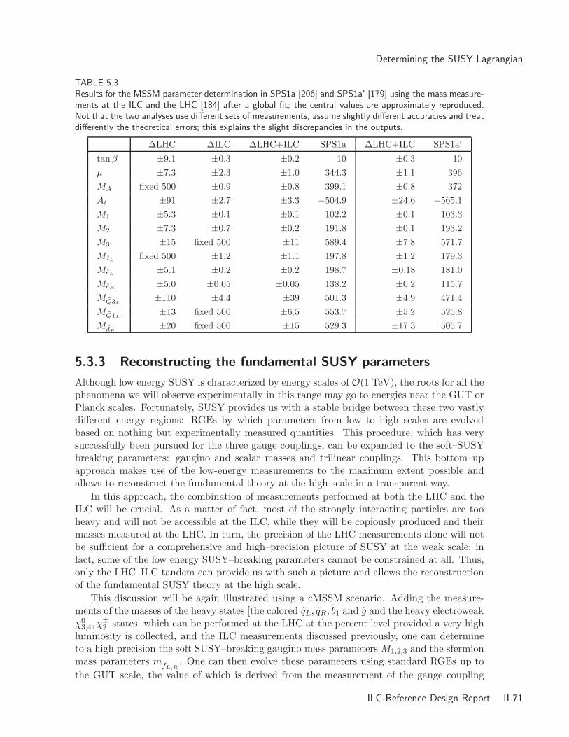
Determining the SUSY Lagrangian
TABLE 5.3Results for the MSSM parameter determination in SPS1a [206] and SPS1a′ [179] using the mass measure-ments at the ILC and the LHC [184] after a global fit; the central values are approximately reproduced.Not that the two analyses use different sets of measurements, assume slightly different accuracies and treatdifferently the theoretical errors; this explains the slight discrepancies in the outputs.
∆LHC ∆ILC ∆LHC+ILC SPS1a ∆LHC+ILC SPS1a′
tan β ±9.1 ±0.3 ±0.2 10 ±0.3 10
µ ±7.3 ±2.3 ±1.0 344.3 ±1.1 396
MA fixed 500 ±0.9 ±0.8 399.1 ±0.8 372
At ±91 ±2.7 ±3.3 −504.9 ±24.6 −565.1
M1 ±5.3 ±0.1 ±0.1 102.2 ±0.1 103.3
M2 ±7.3 ±0.7 ±0.2 191.8 ±0.1 193.2
M3 ±15 fixed 500 ±11 589.4 ±7.8 571.7
MτLfixed 500 ±1.2 ±1.1 197.8 ±1.2 179.3
MeL±5.1 ±0.2 ±0.2 198.7 ±0.18 181.0
MeR±5.0 ±0.05 ±0.05 138.2 ±0.2 115.7
MQ3L±110 ±4.4 ±39 501.3 ±4.9 471.4
MQ1L±13 fixed 500 ±6.5 553.7 ±5.2 525.8
MdR±20 fixed 500 ±15 529.3 ±17.3 505.7
5.3.3 Reconstructing the fundamental SUSY parameters
Although low energy SUSY is characterized by energy scales of O(1 TeV), the roots for all thephenomena we will observe experimentally in this range may go to energies near the GUT orPlanck scales. Fortunately, SUSY provides us with a stable bridge between these two vastlydifferent energy regions: RGEs by which parameters from low to high scales are evolvedbased on nothing but experimentally measured quantities. This procedure, which has verysuccessfully been pursued for the three gauge couplings, can be expanded to the soft–SUSYbreaking parameters: gaugino and scalar masses and trilinear couplings. This bottom–upapproach makes use of the low-energy measurements to the maximum extent possible andallows to reconstruct the fundamental theory at the high scale in a transparent way.
In this approach, the combination of measurements performed at both the LHC and theILC will be crucial. As a matter of fact, most of the strongly interacting particles are tooheavy and will not be accessible at the ILC, while they will be copiously produced and theirmasses measured at the LHC. In turn, the precision of the LHC measurements alone will notbe sufficient for a comprehensive and high–precision picture of SUSY at the weak scale; infact, some of the low energy SUSY–breaking parameters cannot be constrained at all. Thus,only the LHC–ILC tandem can provide us with such a picture and allows the reconstructionof the fundamental SUSY theory at the high scale.
This discussion will be again illustrated using a cMSSM scenario. Adding the measure-ments of the masses of the heavy states [the colored qL, qR, b1 and g and the heavy electroweakχ0
3,4, χ±2 states] which can be performed at the LHC at the percent level provided a very high
luminosity is collected, and the ILC measurements discussed previously, one can determineto a high precision the soft SUSY–breaking gaugino mass parameters M1,2,3 and the sfermionmass parameters mfL,R
. One can then evolve these parameters using standard RGEs up to
the GUT scale, the value of which is derived from the measurement of the gauge coupling
ILC-Reference Design Report II-71

SUPERSYMMETRY
constants at the Giga–Z option of the ILC. In SPS1a′, one obtains (ignoring threshold effects)MGUT = (2.47 ± 0.02) · 1016 GeV, which leads to a common value of α−1
GUT = 24.17 ± 0.06.This is shown in Fig. 5.7, where the thickness of the curves reflect the 1σ errors.
1/Mi [GeV−1]
Q [GeV]
M2
j[103 GeV2]
Q [GeV]
FIGURE 5.7. Evolution from low to high scales of gaugino and scalar mass parameters in the cMSSMpoint SPS1a′; the widths of the bands indicate the 1σ CL [208].
Note that while the parameters are determined accurately in the gaugino and sleptonsectors, the errors are larger for squarks. Nevertheless, one can see that the two sets unifynicely, providing a strong confidence that we are indeed in a cMSSM–type scenario.
One can then derive the basic parameters of the model at the scale MGUT. A global fit ofall the SUSY parameters obtained from measurements at the LHC and the ILC as given inTab. 5.3, can be used to determine the GUT values of the common gaugino and scalar massesm0 and m1/2, the universal trilinear coupling A0 as well as the value of tan β. The result ofa fit performed in Ref. [206] for the SPS1a scenario is shown in Tab. 5.4, with the sign of µfixed to its true value, i.e. µ > 0; for further analyses, see e.g. Ref. [207]. At the LHC, thesefundamental parameters can be determined at the percent level but the ILC improves thedetermination by an order of magnitude; a very accurate picture is achieved when the LHCand ILC data are combined.
TABLE 5.4Summary of the cMSSM fit in SPS1a (with µ > 0 fixed) and SPS1a′ based on the parameter values ofTab. 5.3 at the LHC, ILC and their combination. The same warnings on the differences between the twoanalyses as in the caption of Table 5.3 hold also in this context.
SPS1a LHC ILC LHC+ILC SPS1a′ ∆LHC+ILC
m0 100 100.03± 4.0 100.03± 0.09 100.04 ± 0.08 70 0.2
m1/2 250 249.95± 1.8 250.02± 0.13 250.01 ± 0.11 250 0.2
tan β 10 9.87 ± 1.3 9.98 ± 0.14 9.98 ± 0.14 10 0.3
A0 −100 −99.29± 31.8 −98.26± 4.43 −98.25 ± 4.13 −300 13
II-72 ILC-Reference Design Report
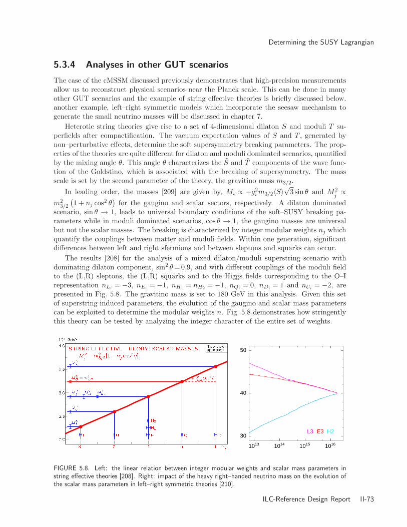
Determining the SUSY Lagrangian
5.3.4 Analyses in other GUT scenarios
The case of the cMSSM discussed previously demonstrates that high-precision measurementsallow us to reconstruct physical scenarios near the Planck scale. This can be done in manyother GUT scenarios and the example of string effective theories is briefly discussed below.another example, left–right symmetric models which incorporate the seesaw mechanism togenerate the small neutrino masses will be discussed in chapter 7.
Heterotic string theories give rise to a set of 4-dimensional dilaton S and moduli T su-perfields after compactification. The vacuum expectation values of S and T , generated bynon–perturbative effects, determine the soft supersymmetry breaking parameters. The prop-erties of the theories are quite different for dilaton and moduli dominated scenarios, quantifiedby the mixing angle θ. This angle θ characterizes the S and T components of the wave func-tion of the Goldstino, which is associated with the breaking of supersymmetry. The massscale is set by the second parameter of the theory, the gravitino mass m3/2.
In leading order, the masses [209] are given by, Mi ∝ −g2im3/2〈S〉
√3 sin θ and M2
j∝
m23/2
(1 + nj cos2 θ
)for the gaugino and scalar sectors, respectively. A dilaton dominated
scenario, sin θ → 1, leads to universal boundary conditions of the soft–SUSY breaking pa-rameters while in moduli dominated scenarios, cos θ → 1, the gaugino masses are universalbut not the scalar masses. The breaking is characterized by integer modular weights nj whichquantify the couplings between matter and moduli fields. Within one generation, significantdifferences between left and right sfermions and between sleptons and squarks can occur.
The results [208] for the analysis of a mixed dilaton/moduli superstring scenario withdominating dilaton component, sin2 θ =0.9, and with different couplings of the moduli fieldto the (L,R) sleptons, the (L,R) squarks and to the Higgs fields corresponding to the O–Irepresentation nLi
= −3, nEi= −1, nH1
= nH2= −1, nQi
= 0, nDi= 1 and nUi
= −2, arepresented in Fig. 5.8. The gravitino mass is set to 180 GeV in this analysis. Given this setof superstring induced parameters, the evolution of the gaugino and scalar mass parameterscan be exploited to determine the modular weights n. Fig. 5.8 demonstrates how stringentlythis theory can be tested by analyzing the integer character of the entire set of weights.
STRING EFFECTIVE THEORY: SCALAR MASSESM2~j = m23=2[1 + n~j cos2 #] Top downapproach
LM2~L-3 U
M2~U
-2 E
M2~EH1
M2H1H2
M2H2
-1 Q0
M2~Q = m23=2
D
m23=2 cos2 #M2~D
1 n~j2.02.53.03.54.0104 GeV2
1013 1014 1015 1016
30
40
50
L3 E3 H2
FIGURE 5.8. Left: the linear relation between integer modular weights and scalar mass parameters instring effective theories [208]. Right: impact of the heavy right–handed neutrino mass on the evolution ofthe scalar mass parameters in left–right symmetric theories [210].
ILC-Reference Design Report II-73

SUPERSYMMETRY
Thus, high-precision measurements at the ILC may provide access to crucial low andhigh–scale parameters which allow to discriminate between various theories beyond the SM.
Another example of model parameterization at the very high scale is provided by left–right symmetric extensions of the SM. The complex structure observed in the neutrino sectorrequires the extension of the MSSM by a superfield including the right–handed neutrino fieldand its scalar partner. If the small neutrino masses are generated by the seesaw mechanism[211], a similar type of spectrum is induced in the scalar sneutrino sector, splitting into lightTeV scale and very heavy masses. The intermediate seesaw scales will affect the evolution ofthe soft mass terms which break the supersymmetry at the high (GUT) scale, particularly inthe third generation with large Yukawa couplings.
If sneutrinos are lighter than charginos and the second lightest neutralino, as encoded inSPS1a′, they decay only to invisible νχ0
1 final states, but sneutrino masses can be measured inchargino decays to sneutrinos and leptons. These decays develop sharp edges at the endpointsof the lepton energy spectrum for charginos produced in e+e− annihilation. Sneutrinos of allthree generations can be explored this way [210]. As seen before, the errors for the first andsecond generation sneutrinos are expected at the level of 400 MeV, doubling for the moreinvolved analysis of the third generation.
This will provide us with the opportunity to measure, indirectly, the intermediate seesawscale of the third generation [210]. This can be illustrated in an SO(10) model in which theYukawa couplings in the neutrino sector are proportional to the up–type quark mass matrix.The masses of the right–handed Majorana neutrinos are hierarchical, ∝ m2
up, and the massof the heaviest neutrino is given by MR3
∼ m2t /mν3 which, for mν3 ∼ 5 × 10⁻² eV, amounts
to ∼ 6 × 10¹⁴ GeV, i.e., a value close to the GUT scale.Since the νR is unfrozen only beyond Q = MνR
the impact of the left–right extension willbe visible in the evolution of the scalar mass parameters only at very high scales. The effect ofνR can be manifest only in the third generation where the Yukawa coupling is large enough;the evolution in the first two generations can thus be used to calibrate the assumption ofuniversality for the scalar mass parameters at the unification scale. In Fig. 5.8 the evolutionof the scalar mass parameters in the third generation and the Higgs mass parameter aredisplayed. The lines include the effects of the right–handed neutrino which induce the kinks.Only the picture including νR, νR is compatible with the assumption of unification.
The kinks in the evolution of M2L3
shift the physical masses [squared] of the τL and ντL
particles of the third generation by the amount ∆ν[MR] compared with the slepton masses ofthe first two generations. The measurement of ∆ν [MR3
] ∝ mν3MR3log(M2
GUT /M2R3
) can beexploited to determine the neutrino seesaw scale of the third generation, MR3
= 3.7–6.9×10¹⁴
GeV [210], in the LR extended SPS1a′ scenario with an initial value of 6 × 10¹⁴ GeV.Thus, this analysis provides us with a unique possibility of indirectly verifying the seesaw
mechanism and estimate of the high-scale νR seesaw mass parameter MR3. This would have
an impact in explaining the baryon asymmetry of the universe if it is triggered by leptogenesisas will be discussed in chapter 7.
II-74 ILC-Reference Design Report

CHAPTER 6
Alternative scenarios
6.1 GENERAL MOTIVATION AND SCENARIOS
Besides supersymmetric models, there are many proposals for physics scenarios beyond theStandard Model. These alternative scenarios involve new dynamics on the electroweak sym-metry breaking and/or new concepts on space–time and their main motivation is, in mostcases, to provide a solution to the naturalness problem. Since this problem is connected withthe stability of the electroweak symmetry breaking scale, and the new ingredients are closelyrelated to the physics of the Higgs sector, its solution necessarily involves new particles and/ornew interactions at the Terascale. Furthermore, these models need to address the questionof the dark matter which calls for a new stable particle with a mass near the EWSB scale.Among the plethora of scenarios which have been proposed, some examples are as follows:
Models with large extra dimensions [58]: If there is an extra dimensional space whereonly gravitons can propagate, the weakness of the gravitational interaction can be explained.In this case, the four–dimensional Planck mass is a fictitious mass scale, and the fundamentalgravity mass scale in the higher dimension can be close to the TeV scale. A characteristiccollider signal is Kaluza–Klein (KK) graviton emission where topologies with missing energyare expected at the LHC and ILC. KK graviton exchange in fermion pair production willplay an important role to confirm the gravitational nature of the new particles.
Warped extra-dimension models [55]: In the setup proposed by Randall and Sundrum(RS), two three–dimensional branes are placed at different points in the fifth dimensionaldirection, and the space–time between two branes is part of a five–dimensional anti–de Sitterspace. In this case, the mass scale on the SM brane is exponentially suppressed compared tothat on the Planck brane. The weakness of gravitation is explained by the suppression of thegraviton wave function at the SM brane. The KK modes of the graviton, however, can couplestrongly to the SM particles, and these may be produced as spin–two resonances at the LHCand ILC. Their effects may also appear indirectly in SM particle production processes. Notethat five–dimensional RS models are dual to strongly coupled four–dimensional models.
Universal extra dimension (UED) models [212]: In these models, all SM particles areassumed to propagate in a flat extra–dimensional space. With a suitable orbifold compact-ification, one can construct a phenomenologically viable model. These models look like abosonic supersymmetric theory since the first KK modes play the role of superpartners inSUSY models but with the wrong spins. One can introduce a KK parity which makes thelightest first KK particle absolutely stable and a potential dark matter candidate.
ILC-Reference Design Report II-75

ALTERNATIVE SCENARIOS
Strong interaction models: Within the SM and its supersymmetric extensions, the Higgsfield is introduced as a fundamental degree of freedom. Dynamical electroweak symmetrybreaking is rooted in new strong interactions, not necessarily involving a Higgs boson [26]. Ifglobal symmetries of these interactions are broken spontaneously, a set of Goldstone bosonswill be generated, such as pions after breaking chiral symmetries in QCD. By absorbingthese Goldstones, longitudinal degrees of freedom and masses are generated for gauge bosons.Several scenarios have been developed along this path quite early [62, 63] as an alternative tothe standard Higgs mechanism and more recently [61] in a variant responding to the successof the light Higgs picture in accounting for the high–precision electroweak data.
Little Higgs models [61]: These are models with a composite Higgs boson but, unliketraditional Technicolor models [63], the dynamical scale is around 10 TeV and the physicalHiggs boson is considered to be a part of composite field. The quadratic divergence of theHiggs boson mass renormalization is canceled at the one–loop level by extra gauge bosons andtop partners with a carefully chosen global and gauge symmetry structure. An interestingclass of little Higgs models are those with T parity [213] in which the new particles can bemuch lighter than 1 TeV without conflict with the precision electroweak data. In particular,the lightest T-odd particle, a heavy photon, can be even lighter than a few hundred GeV.
There is a variety of possibilities in each of the above scenarios. In models with extradimensions, phenomenological implications depend on which particles are allowed to prop-agate in the extra dimensions. The Higgsless model proposed in Ref. [66] is one type of afive–dimensional model. There are also proposals where the idea of extra space dimensions iscombined with low energy supersymmetry. Some models in warped extra dimensions can beconsidered to be the dual description of strongly coupled conformal field theories [214] andcomposite Higgs scenarios have been proposed based on this duality [215].
The above alternative models introduce new particles and interactions at the TeV scaleand new signals are expected at the LHC experiment. If some signals are indeed observed,the nature of the new physics could be determined by various precise measurements at theILC. In this respect, indirect searches for new physics effects in SM and Higgs processes arealso important at the ILC. In the following, typical examples of ILC studies are presented.
6.2 EXTRA DIMENSIONAL MODELS
6.2.1 Large extra dimensions
In the models with large extra dimensions, the effective four–dimensional Planck mass MP
is related to the fundamental gravity mass scale MD in the 4 + δ dimensional space–time byM2P = VδM
2+δD where Vδ is the volume of the extra–dimensional space. For example, taking
MD = 1 TeV, the size of the extra dimension is 0.1 mm to 1 fm for δ = 2 to 6. The KKmodes of the graviton have, therefore, an almost continuous spectrum.
At the ILC, the observation of a single photon with missing energy due to the emission ofa KK graviton in the reaction e+e− → GKKγ is a robust signal of the model. The sensitivityto the scale MD in this channel is shown in Table 6.1 for polarized and unpolarized e± beams.Beam polarization is very effective in this case as the main background process, e+e− → ννγ,can be suppressed significantly. The search limit for the scale MD is similar to that obtainedin gluon and KK graviton emission at the LHC. Note that there are severe cosmologicaland astrophysical [216] bounds on the mass MD in this scenario; a recent analysis [217]
II-76 ILC-Reference Design Report

Extra dimensional models
of astrophysical data sets a lower limit of several hundred TeV in the case of two extradimensions. The limit is weaker for a larger number of extra dimensions and the constraintsare not strong for δ ≥ 4.
TABLE 6.1The sensitivity at the 95% CL in the mass scale MD (in TeV) for direct graviton production in the polarizedand unpolarized e+e− → γGKK process for various δ values assuming a 0.3% normalization error [7].
δ 3 4 5 6
MD(Pe− = Pe+ = 0) 4.4 3.5 2.9 2.5
MD(Pe− = 0.8) 5.8 4.4 3.5 2.9
MD(Pe− = 0.8,Pe+ = 0.6) 6.9 5.1 4.0 3.3
Once the missing energy signal is observed, the next step would be to confirm its gravita-tional nature and determine the number of extra dimensions. The ILC will play an essentialrole here. The number of extra dimensions can be determined from the energy dependenceof the production cross section. In the left–hand side of Fig. 6.1, it is shown that its mea-surement at two collider energies,
√s = 500 GeV and 800 GeV, can discriminate between
scenarios with different numbers of extra dimensions. Additional information on the numberof extra dimensions can also be obtained from the missing mass distribution.
√s (GeV)
σ γG (f
b)
4
56789
10
20
30
40
5060708090
100
200
400 450 500 550 600 650 700 750 800 850 900
FIGURE 6.1. Left: determination of the number of extra-dimensions at the ILC at two center of massenergies
√s = 500 and 800 GeV [218]. Right: the differential azimuthal asymmetry distribution for
e+e− → `+`− at 500 GeV ILC with 500 fb−1 data in the SM (histogram) and in the LED model with acut–off of 1.5 TeV (data points); e± are assumed to be 80% and 60% polarized, respectively [219].
An alternative signal for the presence of extra dimensions is provided by KK–gravitonexchange in processes such as e+e− → f f . The mass reach in this channel is similar to thatobtained in KK–graviton emission. Since many new physics models can generate deviations inthis reaction, it is important to discriminate the extra–dimensional model from other scenar-ios. s–channel KK–graviton exchange has the characteristic signature of spin–two particlein the angular distributions of the e+e− → f f ,WW and HH production processes [220].Furthermore, if both electron and positron are transversely polarized, the azimuthal asym-metry distribution provides a powerful tool to identify the spin–two nature of the virtuallyexchanged particle [17, 219] as shown in the right–hand side of Fig. 6.1.
ILC-Reference Design Report II-77

ALTERNATIVE SCENARIOS
6.2.2 Warped extra dimensions
In the original proposal of Randall and Sundrum [55], only the graviton was assumed topropagate in the extra–dimensional space and the SM fields were confined on the TeV brane.In this model, the mass scales of the dimensionful parameters in the action are set by thePlanck scale, but the physical mass scales on the TeV (or SM) brane are reduced by the warpfactor of e−πkrc where krc ∼ 11 to explain the hierarchy between the weak and Planck scales.A characteristic signal of this extension is the presence of the graviton KK modes near theTeV scale. In fact, the model is specified by two parameters, for instance, the mass of the firstKK mode and k/M∗ where M∗ is the four–dimensional reduced Planck mass. KK gravitonresonances can be searched for through the Drell–Yan process at the LHC and the mass reachcan be 3–4 TeV, covering most of the interesting parameter space of the model [221].
If such resonances are indeed observed at the LHC, one needs to establish their gravita-tional nature. The spin of the resonance can be determined from the angular distributionof the final lepton pairs at the LHC and ILC [221, 222]. The search reach through contactinteractions at the ILC with a c.m. energy of 500 GeV is similar to the LHC direct searchreach and a 1 TeV ILC can significantly extend the discovery limit [15].
Another important property which has to be verified is the universal structure of thegraviton couplings to other particles. For this purpose, the branching ratios of the resonanceshave to be determined precisely. An ultimate confirmation of the model would be providedby the s–channel production of the KK graviton state at the ILC as shown in Fig. 6.2. Fromline–shape analyses, the two independent parameters, the first KK mode mass and the ratiok/M∗, can be precisely determined along with the various decay branching ratios.
FIGURE 6.2. Graviton resonance production at the ILC in e+e−→µ+µ− in the RS model with the massof the first KK mode taken to be 500 GeV; the exchange of a KK tower is included and the ever wideningresonances correspond to increasing the value of k/M∗ in the range of 0.01–0.1. From Ref. [221].
In RS models, one would expect the presence of a radion which will mix with the Higgs bo-son whose properties could be significantly altered. The Higgs couplings to various particles,for instance, could be reduced at the level of a few 10%. These effects can be easily identifiedwith the precision ILC measurements as discussed in chapter 2. The radion has substantialcouplings to the W/Z bosons and can be produced in the Higgs–strahlung e+e− → φZ or
II-78 ILC-Reference Design Report
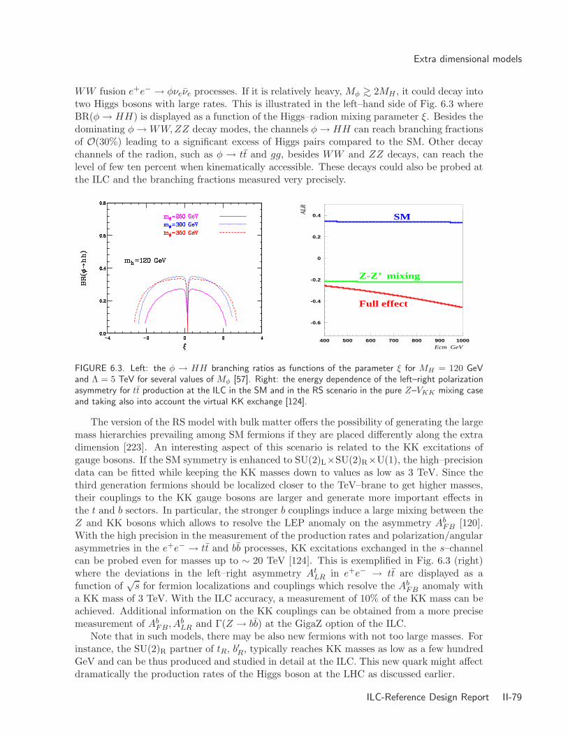
Extra dimensional models
WW fusion e+e− → φνeνe processes. If it is relatively heavy, Mφ >∼ 2MH , it could decay intotwo Higgs bosons with large rates. This is illustrated in the left–hand side of Fig. 6.3 whereBR(φ → HH) is displayed as a function of the Higgs–radion mixing parameter ξ. Besides thedominating φ → WW,ZZ decay modes, the channels φ → HH can reach branching fractionsof O(30%) leading to a significant excess of Higgs pairs compared to the SM. Other decaychannels of the radion, such as φ → tt and gg, besides WW and ZZ decays, can reach thelevel of few ten percent when kinematically accessible. These decays could also be probed atthe ILC and the branching fractions measured very precisely.
-0.6
-0.4
-0.2
0
0.2
0.4
400 500 600 700 800 900 1000Ecm GeV
ALR
Full effect
SM
Z-Z’ mixing
FIGURE 6.3. Left: the φ → HH branching ratios as functions of the parameter ξ for MH = 120 GeVand Λ = 5 TeV for several values of Mφ [57]. Right: the energy dependence of the left–right polarizationasymmetry for tt production at the ILC in the SM and in the RS scenario in the pure Z–VKK mixing caseand taking also into account the virtual KK exchange [124].
The version of the RS model with bulk matter offers the possibility of generating the largemass hierarchies prevailing among SM fermions if they are placed differently along the extradimension [223]. An interesting aspect of this scenario is related to the KK excitations ofgauge bosons. If the SM symmetry is enhanced to SU(2)L×SU(2)R×U(1), the high–precisiondata can be fitted while keeping the KK masses down to values as low as 3 TeV. Since thethird generation fermions should be localized closer to the TeV–brane to get higher masses,their couplings to the KK gauge bosons are larger and generate more important effects inthe t and b sectors. In particular, the stronger b couplings induce a large mixing between theZ and KK bosons which allows to resolve the LEP anomaly on the asymmetry Ab
FB [120].With the high precision in the measurement of the production rates and polarization/angularasymmetries in the e+e− → tt and bb processes, KK excitations exchanged in the s–channelcan be probed even for masses up to ∼ 20 TeV [124]. This is exemplified in Fig. 6.3 (right)where the deviations in the left–right asymmetry At
LR in e+e− → tt are displayed as afunction of
√s for fermion localizations and couplings which resolve the Ab
FB anomaly witha KK mass of 3 TeV. With the ILC accuracy, a measurement of 10% of the KK mass can beachieved. Additional information on the KK couplings can be obtained from a more precisemeasurement of Ab
FB, AbLR and Γ(Z → bb) at the GigaZ option of the ILC.
Note that in such models, there may be also new fermions with not too large masses. Forinstance, the SU(2)R partner of tR, b′R, typically reaches KK masses as low as a few hundredGeV and can be thus produced and studied in detail at the ILC. This new quark might affectdramatically the production rates of the Higgs boson at the LHC as discussed earlier.
ILC-Reference Design Report II-79

ALTERNATIVE SCENARIOS
6.2.3 Universal extra dimensions
Universal extra dimensions (UED) [212] is the model which resembles the most to the originalNordstrom–Kaluza–Klein scenario. All SM particles are assumed to propagate in a flat extra–dimensional space which is compactified to an orbifold. In the minimal version, the extraone–dimensional space is compactified in the form of an S1/Z2 orbifold, where a circle S1
is divided in half by Z2 projection. Viewed as a four dimensional theory, the UED modelintroduces a Kaluza–Klein tower for each SM particle. The common mass of the nth KK statesis roughly given by n/R where R is the compactification radius, but radiative corrections andboundary terms lift the initial mass degeneracy of the nth KK states.
In UED models, momentum conservation in the fifth dimension is replaced by a conservedparity, called KK–parity [224, 225]. The zero modes, i.e. the SM particles, are even underthis parity but the lightest massive modes are odd. This has the major consequence thatthe lightest KK particle (LKP), which in general corresponds to the KK hypercharge gaugeboson, is absolutely stable. It gives missing transverse energy signals at colliders and is agood dark matter candidate as will be discussed in chapter 7. Another important consequenceof this parity is that n = 1 KK particles are only produced in pairs. This suppresses theirvirtual corrections to SM processes, allowing the UED scale 1/R to be as low as 300 GeVwithout conflicting with high–precision electroweak data.
From the previous discussion, one concludes that the situation in UED models is quiteanalogous to the minimal supersymmetric SM extension with conserved R–parity, exceptthat here, the lightest particle is a spin–one particle, a heavy photon. Thus, if only the firstmassive KK modes are produced, UED models would look very much like a subset of SUSYmodels in terms of their collider signatures. Even if one detects a few of the second level KKmodes, it is not obvious that this will discriminate the signatures from an extended SUSYmodel. The crucial discriminators, of course, are the spins of the heavy partner particles.At the LHC, distinguishing these spins is a significant experimental challenge. The ILCwill play an important role in this context as the spin difference between superpartners andKK excitations can be determined in detailed angular distribution studies and thresholdscans. This is exemplified in Fig. 6.4 where the threshold excitation curve and the angulardistribution in the case of e+e− → µ+
R1µ−R1 for the first muon KK excitation in UED models
is compared to smuon pair production in the MSSM, e+e− → µ+Rµ−
R [187].
500 600 700 800 900 1000 1100 1200√s (GeV)
0
50
100
150e
+e
− → ∼µ+R
∼µ−R
σ (fb) :
e+e
− → µ+R1
µ−R1
4 × σ ( ∼µ+R
∼µ−R
)
σ ( µ+R1
µ−R1
)
m∼µR= mµ
R1= 300 GeV
(a)
-1 -0.5 0 0.5 1cosθ
0
10
20
30
40
50
60
70
e+e
− → ∼µ+R
∼µ−R
e+e
− → µ+R1
µ−R1
dσdcosθ :
SUSY : ∼µR
UED : µR1
ILC [1 TeV]
CLIC [3 TeV]
[arbitrary normalization]
(b)
FIGURE 6.4. The threshold excitation for smuons (a) and the angular distribution (b) in the case of smuonsin the MSSM and the first KK excitation µ±
R1 in UED in pair production at the ILC; from Ref. [187].
II-80 ILC-Reference Design Report

Strong interaction models
6.3 STRONG INTERACTION MODELS
6.3.1 Little Higgs models
To interpret the Higgs boson as a (pseudo-)Goldstone boson has been a very attractive ideafor a long time. The interest in this picture has been renewed within the little Higgs scenar-ios [61], that have recently been developed to generate the electroweak symmetry breakingdynamically by new strong interactions. Little Higgs models (LHMs) are based on a complexsystem of symmetries and symmetry breaking mechanisms. Three points are central in real-izing the idea: (i) the Higgs field is a Goldstone field associated with the breaking of a globalsymmetry G at an energy scale of order Λs ∼ 4πf ∼ 10 to 30 TeV, with f characterizingthe scale of the symmetry breaking parameter; (ii) in the same step, the gauge symmetryG0 ⊂ G is broken down to the SM gauge group, generating masses for heavy vector bosonsand fermions which cancel the standard quadratic divergencies in the radiative corrections tothe light Higgs mass; since the masses of these new particles are generated by the breaking ofthe gauge symmetry G0 they are of the intermediate size M ∼ gf ∼ 1 to 3 TeV; (iii) the Higgsbosons acquires a mass finally through radiative corrections at the standard electroweak scaleof order v ∼ g2f/4π ∼ 100 to 300 GeV.
Thus, three characteristic scales are encountered in these models: the strong interactionscale Λs, the new mass scale M and the electroweak breaking scale v, ordered in the hierarchi-cal chain Λs M v. The light Higgs boson mass is protected at small value by requiringthe collective breaking of two symmetries. In contrast to the boson–fermion symmetry thatcancels quadratic divergencies in supersymmetry, the cancellation in LHMs operates in thebosonic and fermionic sectors individually, the cancellation ensured by the symmetries amongthe couplings of the SM fields and new fields to the Higgs field.
A generic feature of LHMs is the existence of extra gauge bosons, Higgs particles andpartners of the top quark. The masses of these new particles are constrained by electroweakprecision measurements. Although the precise values depend on the specific model underconsideration, these are usually beyond a few TeV, so that their direct production is kine-matically not accessible at the ILC. If one introduce T–parity, these masses can be belowthe TeV scale, but T–odd particles should be pair produced. Even if the new particles arebeyond the kinematical reach of the ILC, indirect searches for effects of LHMs is possible inSM processes such as e+e− → f f , tt, ZH and γγ → H.
An example of indirect search of the new states at the ILC is shown in the left–handside of Fig. 6.5. The figure displays the limit on the vev f associated with SU(5) → SO(5)symmetry breaking in LHMs as derived from the e+e− → f f processes with a center of massenergy
√s = 500 GeV and an integrated luminosity of 500 fb−1. Two new mixing angles
s and s′ specify the gauge symmetry breaking of [SU(2) × U(1)]2 → SU(2)L × U(1)Y. Forcomparison, the LHC search reach for the heavy gauge boson ZH is also shown. As canbe seen, the indirect searches at the ILC can extend the LHC search limit substantially. Asimilar search can be performed in the e+e− → ZH process but with less sensitivity.
In order to cancel the quadratic divergence in the Higgs mass in LHMS, the top quarksector has to be extended. The ordinary top quark is identified as one light combinationof the extended top sector so that there could be sizable deviations in the top coupling toW/Z bosons. In Fig. 6.5 (right), the correction to the ttZ coupling is shown in the case ofLHMs with T–parity. The displayed ILC search limit indicates that most of the interestingparameter region is covered by future high–precision top quark measurements.
ILC-Reference Design Report II-81

ALTERNATIVE SCENARIOS
0.2
0.3
0.4
0.5
0.6
0.7
0.8
0.9
1
1 2 3 4 5 6 7 8 9 10
s
f (TeV)
5 σ contours with MAH→ ∞ at √s = 500 GeV
SEARCHREACH
BY LEP IIEXCLUDED
LHC
ILC s’= √3/5
s’ = 0.50
s’= s
s’ = s/2
FIGURE 6.5. Left: the ILC search reach in LHMs, as derived from the process e+e− → f f , is comparedto the LHC reach in heavy Z ′ boson searches; the decoupling limit of the heavy photon is taken [226].Right: the corrections to the ttZ coupling in LHMs with conserved T–parity for two values of the heavytop quark partner compared to the (super)LHC and ILC sensitivities [227].
Even if T–parity is not imposed, a pseudo–axion might be light enough to be accessible atthe ILC in the case where LHMs possess a spontaneously broken approximate U(1) symmetryas in the simplest model [228]. In such a case the pseudo–axion η could be produced inassociation with the Higgs boson, e+e− → Hη and would decay via η → HZ. This isexemplified in Fig. 6.6 (left) where the cross section for the e+e− → ηH → HHZ process isshown as a function of
√s for scenarios with and without the contribution of a Z ′ boson [64].
The new contributions increase the ZHH rate by an order of magnitude compared to theSM. A relatively light η boson could also be produced in association with top quark pairs,e+e− → ttη and the signal in which the η resonance dominantly decays into bb pairs couldbe easily observed at the ILC as shown in Fig. 6.6 (right) for several Mη values.
no Z′
with Z′
SM
σ(e+e− → η
∗H → ZHH) [fb]
400 600 800 1000
0.5
1
1.5
√s [GeV]
FIGURE 6.6. Left: the cross section of double Higgs production with and without Z ′ exchange comparedwith the SM prediction in the simplest LHM for MH ∼ 130 GeV and Mη ∼ 300 GeV. Right: thereconstructed bb invariant mass in the process e+e− → ttη → ttbb compared to the SM background; thepeaks correspond to Z, H production and to the η resonance for several Mη values. From Ref. [64].
II-82 ILC-Reference Design Report

Strong interaction models
6.3.2 Strong electroweak symmetry breaking
If no Higgs boson will be observed with mass below 1 TeV, quantum–mechanical unitaritydemands strong interactions between the electroweak gauge bosons, becoming effective atenergies (8π/
√2GF )1/2 ' 1.2 TeV, to damp the growth of the amplitudes for (quasi–)elastic
massive gauge boson scattering processes [38].
As discussed in chapter 3, the new interactions between the weak bosons can be expandedin a series of effective interaction terms with rising dimensions [130]. Scattering amplitudesare expanded correspondingly in a series characterized by the energy coefficients s/Λ2
∗. De-manding CP and isospin invariance, for instance, only two new dimension–four interactionterms (out of the 10 terms present in the general case) must be included in the expansion,L4 and L5, with coefficients α4,5 = v2/Λ2
∗4,5 with scale parameters bounded from above bythe value 4πv ∼ 3 TeV. The parameters αi can be measured in the quasi–elastic V V scatter-ing processes e+e− → ``V V and triple gauge boson production e+e− → V V V , as the newinteraction terms affect the total cross sections and the final state distributions.
As can be seen from Figs. 3.4 and 3.5 of chapter 3, at√
s = 1 TeV with 1 ab−1 data,the entire range of Λ∗ values can be covered, Λ∗ ≤ 4πv ' 3 TeV. These values can beconveniently re–expressed in terms of the maximal mass of the heavy resonances associatedwith the new interactions the measurement can be sensitive to, under the most favorableconditions; Fig. 6.7 (left). In Table 6.2, displayed are the combined results obtained in thefull analysis of Ref. [131] for the sensitivity on the scale Λ∗ for all possible spin/isospinchannels. In the left–hand side of the table, a conserved SU(2)c is assumed and in this case,only the channels with even I+J couple to weak boson pairs; in the right–hand side, shown arethe results without this constraint. In each case, a single resonance with maximal couplingwas assumed to be present. As one can see, scales from ∼ 1.5 to ∼ 6 TeV can be probed.
TABLE 6.2Accessible scales Λ∗ in TeV for all possible spin/isospin channels from a complete analysis of vector bosonscattering processes at 1 TeV the ILC, assuming a single resonance with optimal properties [131]. Thenumbers in the left–(right–)hand side are with (without) assuming the custodial symmetry.
Spin I=0 I=1 I=2 I=0 I=1 I=2
0 1.55 – 1.95 1.39 1.55 1.951 – 2.49 – 1.74 2.67 –2 3.29 – 4.30 3.00 3.01 5.84
Alternatively, when resonances below the scale Λ∗ are present, the vector boson pairproduction amplitude can be unitarised by a Omnes rescattering factor with one contributionreproducing the low energy theorem δLET(s) = s/(8Λ2
EWSB) for Goldstone boson scatteringat threshold far below any resonance and a second contribution from a resonance δρ(s) =3π/8 · (tanh(s−M2
ρ )/(MρΓρ) + 1). A study performed in Ref. [229] has shown that W+W−
production at the ILC with√
s = 800 GeV and L = 500 fb−1 is competitive with the LHC.As shown in the right–hand side of Fig. 6.7, there is a 6σ exclusion limit for the LET andone can exclude a ρ–like resonance of 2.5 (1.6) TeV at the 16 (33)σ level.
A concrete example of models with a strong EWSB sector is the BESS model [231], whichincludes most Technicolor models [63]. It assumes a triplet of new vector resonances V ±,0,similar to the ρ or techni–ρ, which mix with the W/Z bosons with a mixing ∝ g/g′′, whereg′′ is the self–coupling of the V ±,0 state. The f fV ±,0 couplings are determined by a second
ILC-Reference Design Report II-83
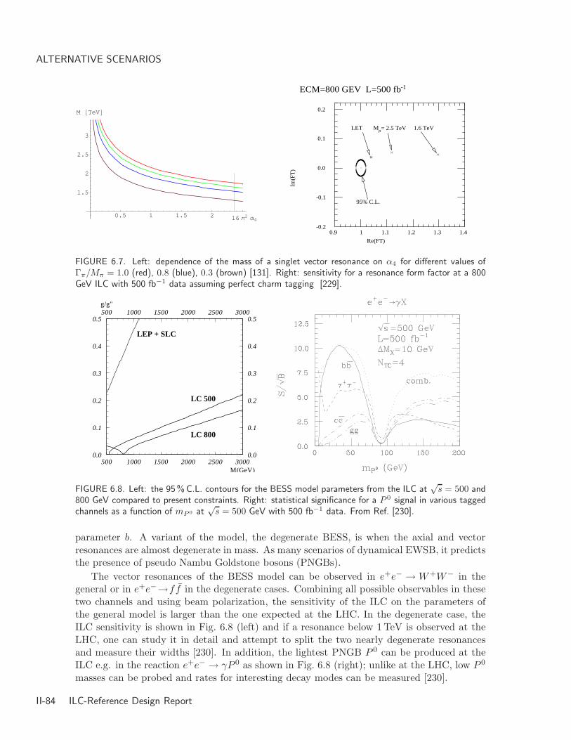
ALTERNATIVE SCENARIOS
0.5 1 1.5 2 16 Π2 Α4
1.5
2
2.5
3
M @TeVD
ECM=800 GEV L=500 fb-1
Re(FT)
Im
(FT
)
5
0.9 1 1.1 1.2 1.3 1.4-0.2
-0.1
0.0
0.1
0.2
55
5
5
1.6 TeV Mρ= 2.5 TeV LET
95% C.L.
555555555555555555555555555555555555555555555555555555555555555555555555555555555555555555555555555555555555555555555555555555555555555555555555555555555555555555555555555555555555555555555555555555555555555555555555555555555555555555555555555555555555555555555555555555555
555555555555555555555555555
55555555555555555555555555555555555555555555555555555555555555555555555555555555555555555555555555555555555555555555555555555555555555555555555555555555555555555555555555555555555555555555555555555555
5555555555555555555555555555555555555555555555555555555555555555555555555555555555555555555555555555
FIGURE 6.7. Left: dependence of the mass of a singlet vector resonance on α4 for different values ofΓπ/Mπ = 1.0 (red), 0.8 (blue), 0.3 (brown) [131]. Right: sensitivity for a resonance form factor at a 800GeV ILC with 500 fb−1 data assuming perfect charm tagging [229].
500 1000 1500 2000 2500 30000.0
0.1
0.2
0.3
0.4
0.5500 1000 1500 2000 2500 3000
0.0
0.1
0.2
0.3
0.4
0.5
M(GeV)
g/g"
LC 500
LEP + SLC
LC 800
FIGURE 6.8. Left: the 95% C.L. contours for the BESS model parameters from the ILC at√
s = 500 and800 GeV compared to present constraints. Right: statistical significance for a P 0 signal in various taggedchannels as a function of mP 0 at
√s = 500 GeV with 500 fb−1 data. From Ref. [230].
parameter b. A variant of the model, the degenerate BESS, is when the axial and vectorresonances are almost degenerate in mass. As many scenarios of dynamical EWSB, it predictsthe presence of pseudo Nambu Goldstone bosons (PNGBs).
The vector resonances of the BESS model can be observed in e+e− → W+W− in thegeneral or in e+e−→f f in the degenerate cases. Combining all possible observables in thesetwo channels and using beam polarization, the sensitivity of the ILC on the parameters ofthe general model is larger than the one expected at the LHC. In the degenerate case, theILC sensitivity is shown in Fig. 6.8 (left) and if a resonance below 1 TeV is observed at theLHC, one can study it in detail and attempt to split the two nearly degenerate resonancesand measure their widths [230]. In addition, the lightest PNGB P 0 can be produced at theILC e.g. in the reaction e+e− → γP 0 as shown in Fig. 6.8 (right); unlike at the LHC, low P 0
masses can be probed and rates for interesting decay modes can be measured [230].
II-84 ILC-Reference Design Report

Strong interaction models
6.3.3 Higgsless scenarios in extra dimensions
Also in theories with extra space dimensions, the electroweak symmetry can be broken with-out introducing a fundamental scalar field, leading to Higgsless theories [66]. Since in five–dimensional theories the wave functions are expanded by a fifth component, the electroweaksymmetry can be broken by applying appropriately chosen boundary conditions to this fieldcomponent. This scalar component of the original five–dimensional gauge field is absorbedto generate the massive KK towers of the gauge fields in four dimensions. The additionalexchange of these towers in WW scattering damps the scattering amplitude of the SM andallows, in principle, to extend the theory to energies beyond the O(1) TeV unitarity bound ofHiggsless scenarios. However, it is presently unclear whether realistic models of this type canbe constructed that give rise to small enough elastic WW scattering amplitudes compatiblewith perturbative unitarity [232].
Higgsless models can be best tested at the ILC if the energy is pushed to its maximum.Unlike for Technicolor models, one expects that the masses of the new vector bosons, collec-tively called V1, are below the TeV scale and thus kinematically accessible. In this case, theycan be produced in the W/Z fusion processes e+e− → V ±
1 e∓νe and e+e− → V 01 νeνe for the
charged and neutral states, respectively. The cross sections for these processes, as well as theone for the associated production process e+e− → V ±W∓, are shown as a function of the V1
mass in the left–hand side of Fig. 6.9 for c.m. energies of√
s = 500 GeV and√
s = 1 TeVand compared to the SM W±W∓Z continuum background [233]. One can see that the ratesare rather large, exceeding the femtobarn level for V1 masses close to MV1
= 800 GeV at a 1TeV c.m. energy, before experimental cuts and efficiencies are applied. Thanks to the cleanenvironment, the dominant hadronic decays of the W/Z bosons can be used and the invariantmasses of the V1 resonances can be easily reconstructed. This provides an extra handle forsuppressing the SM background as shown in the right–hand side of Fig. 6.9 where the WZinvariant mass distribution for the signal of Higgsless models and the SM background arecompared for the same two c.m. energies and several values of the resonance masses. Thus,the ILC has a real potential to test some of the generic predictions of Higgsless models.
FIGURE 6.9. Left: the production cross sections for the new gauge bosons V1 and the continuum SMbackground at the ILC. Right: the WZ invariant mass distribution for the signal in Higgsless models andthe SM background. In both cases, the c.m. energy is
√s = 500 GeV and 1 TeV. From Ref. [233].
ILC-Reference Design Report II-85
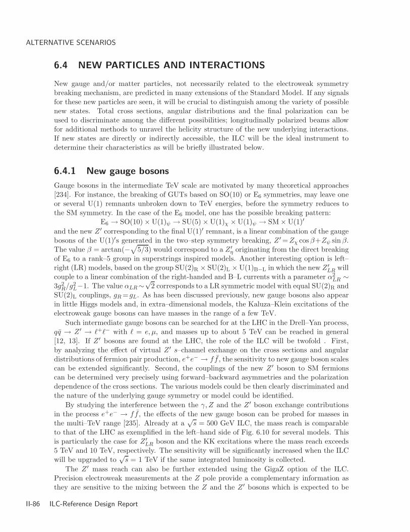
ALTERNATIVE SCENARIOS
6.4 NEW PARTICLES AND INTERACTIONS
New gauge and/or matter particles, not necessarily related to the electroweak symmetrybreaking mechanism, are predicted in many extensions of the Standard Model. If any signalsfor these new particles are seen, it will be crucial to distinguish among the variety of possiblenew states. Total cross sections, angular distributions and the final polarization can beused to discriminate among the different possibilities; longitudinally polarized beams allowfor additional methods to unravel the helicity structure of the new underlying interactions.If new states are directly or indirectly accessible, the ILC will be the ideal instrument todetermine their characteristics as will be briefly illustrated below.
6.4.1 New gauge bosons
Gauge bosons in the intermediate TeV scale are motivated by many theoretical approaches[234]. For instance, the breaking of GUTs based on SO(10) or E6 symmetries, may leave oneor several U(1) remnants unbroken down to TeV energies, before the symmetry reduces tothe SM symmetry. In the case of the E6 model, one has the possible breaking pattern:
E6 → SO(10) × U(1)ψ → SU(5) × U(1)χ × U(1)ψ → SM × U(1)′
and the new Z ′ corresponding to the final U(1)′ remnant, is a linear combination of the gaugebosons of the U(1)′s generated in the two–step symmetry breaking, Z ′ =Zχ cos β+Zψ sin β.The value β = arctan(−
√5/3) would correspond to a Z ′
η originating from the direct breakingof E6 to a rank–5 group in superstrings inspired models. Another interesting option is left–right (LR) models, based on the group SU(2)R × SU(2)L × U(1)B−L in which the new Z ′
LR willcouple to a linear combination of the right-handed and B–L currents with a parameter α2
LR ∼3g2R/g2
L−1. The value αLR∼√
2 corresponds to a LR symmetric model with equal SU(2)R andSU(2)L couplings, gR=gL. As has been discussed previously, new gauge bosons also appearin little Higgs models and, in extra–dimensional models, the Kaluza–Klein excitations of theelectroweak gauge bosons can have masses in the range of a few TeV.
Such intermediate gauge bosons can be searched for at the LHC in the Drell–Yan process,qq → Z ′ → `+`− with ` = e, µ, and masses up to about 5 TeV can be reached in general[12, 13]. If Z ′ bosons are found at the LHC, the role of the ILC will be twofold . First,by analyzing the effect of virtual Z ′ s–channel exchange on the cross sections and angulardistributions of fermion pair production, e+e− → f f , the sensitivity to new gauge boson scalescan be extended significantly. Second, the couplings of the new Z ′ boson to SM fermionscan be determined very precisely using forward–backward asymmetries and the polarizationdependence of the cross sections. The various models could be then clearly discriminated andthe nature of the underlying gauge symmetry or model could be identified.
By studying the interference between the γ, Z and the Z ′ boson exchange contributionsin the process e+e− → f f , the effects of the new gauge boson can be probed for masses inthe multi–TeV range [235]. Already at a
√s = 500 GeV ILC, the mass reach is comparable
to that of the LHC as exemplified in the left–hand side of Fig. 6.10 for several models. Thisis particularly the case for Z ′
LR boson and the KK excitations where the mass reach exceeds5 TeV and 10 TeV, respectively. The sensitivity will be significantly increased when the ILCwill be upgraded to
√s = 1 TeV if the same integrated luminosity is collected.
The Z ′ mass reach can also be further extended using the GigaZ option of the ILC.Precision electroweak measurements at the Z pole provide a complementary information asthey are sensitive to the mixing between the Z and the Z ′ bosons which is expected to be
II-86 ILC-Reference Design Report
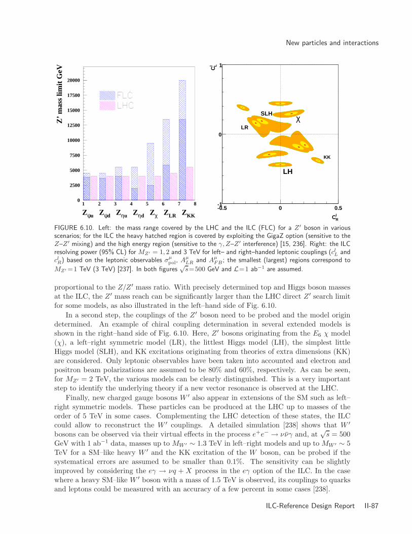
New particles and interactions
0
2500
5000
7500
10000
12500
15000
17500
20000
1 2 3 4 5 6 7 8
Zψu Zψd Zηu Zηd Zχ ZLR ZKK
Z’
mas
s lim
it G
eV
lRC
-0.5 0 0.5l L
C
-1
0
1
LH
LR
KK
χSLH
FIGURE 6.10. Left: the mass range covered by the LHC and the ILC (FLC) for a Z ′ boson in variousscenarios; for the ILC the heavy hatched region is covered by exploiting the GigaZ option (sensitive to theZ–Z ′ mixing) and the high energy region (sensitive to the γ, Z–Z ′ interference) [15, 236]. Right: the ILCresolving power (95% CL) for MZ′ = 1, 2 and 3 TeV for left– and right–handed leptonic couplings (cl
L andclR) based on the leptonic observables σµ
pol, AµLR and Aµ
FB ; the smallest (largest) regions correspond to
MZ′ =1 TeV (3 TeV) [237]. In both figures√
s=500 GeV and L=1 ab−1 are assumed.
proportional to the Z/Z ′ mass ratio. With precisely determined top and Higgs boson massesat the ILC, the Z ′ mass reach can be significantly larger than the LHC direct Z ′ search limitfor some models, as also illustrated in the left–hand side of Fig. 6.10.
In a second step, the couplings of the Z ′ boson need to be probed and the model origindetermined. An example of chiral coupling determination in several extended models isshown in the right–hand side of Fig. 6.10. Here, Z ′ bosons originating from the E6 χ model(χ), a left–right symmetric model (LR), the littlest Higgs model (LH), the simplest littleHiggs model (SLH), and KK excitations originating from theories of extra dimensions (KK)are considered. Only leptonic observables have been taken into accounted and electron andpositron beam polarizations are assumed to be 80% and 60%, respectively. As can be seen,for MZ′ = 2 TeV, the various models can be clearly distinguished. This is a very importantstep to identify the underlying theory if a new vector resonance is observed at the LHC.
Finally, new charged gauge bosons W ′ also appear in extensions of the SM such as left–right symmetric models. These particles can be produced at the LHC up to masses of theorder of 5 TeV in some cases. Complementing the LHC detection of these states, the ILCcould allow to reconstruct the W ′ couplings. A detailed simulation [238] shows that W ′
bosons can be observed via their virtual effects in the process e+e− → ννγ and, at√
s = 500GeV with 1 ab−1 data, masses up to MW ′ ∼ 1.3 TeV in left–right models and up to MW ′ ∼ 5TeV for a SM–like heavy W ′ and the KK excitation of the W boson, can be probed if thesystematical errors are assumed to be smaller than 0.1%. The sensitivity can be slightlyimproved by considering the eγ → νq + X process in the eγ option of the ILC. In the casewhere a heavy SM–like W ′ boson with a mass of 1.5 TeV is observed, its couplings to quarksand leptons could be measured with an accuracy of a few percent in some cases [238].
ILC-Reference Design Report II-87

ALTERNATIVE SCENARIOS
6.4.2 Exotic fermions
Many theories beyond the SM such as GUTs or extra–dimensional require the existenceof new matter particles with the possibility of new interactions not contained in the SM;for a review, see e.g. Ref. [239]. Examples of new elementary fermions include sequentialfourth generation fermions, vector–like fermions with both left– and right–handed compo-nents in weak isodoublets, mirror fermions which have the opposite chiral properties as theSM fermions and isosinglet fermions such as the SO(10) Majorana neutrino. Exotic fermions,i.e. fermions that have the usual lepton/baryon but non-canonical SU(2)L × U(1)Y quantumnumbers, occur naturally in GUT models that contain a single representation into which acomplete generation of SM quarks and leptons can be embedded. For instance, in the E6
group, each fermion generation lies in the 27 representation, which contains 12 new fermionsin addition to the 15 chiral fermions of the SM. It is conceivable that these new fermionsacquire masses not much larger than the EWSB scale, if these masses are protected by somesymmetry. In fact, this is necessary if the associated new gauge bosons are relatively light.
Except for singlet neutrinos, the new fermions couple to the photon and/or to the weakgauge bosons W/Z with full strength; these couplings allow for pair production, e+e− → FF ,with practically unambiguous cross sections and, masses very close to the kinematical limit,mF ∼ 1
2
√s, can be probed; see Fig. 6.11 (left). In general, the new fermions will mix with
their SM light partners which have the same conserved quantum numbers. This mixing,which is expected to be small ξ <∼ 0.1 from LEP constraints, gives rise to new currents whichdetermine the decay pattern of the heavy fermions, F → fZ/f ′W .
The mixing also allows for the single production of the new fermions, e+e− → F f . Inthe case of quarks and second/third generation leptons, single production proceeds onlyvia s–channel Z exchange and the rates are moderate. For the first generation neutraland charged leptons, one has additional t–channel exchanges which significantly increase theproduction cross sections; see Fig. 6.11 (right). For not too small mixing, lepton massesclose to the center of mass energy can be produced. A full simulation [240] of the processese+e− → Nνe → e±W∓νe and e+e− → E±e∓ → e±e∓Z, taking into account the dominantbackgrounds and detector efficiencies, shows that for MN,E = 350 GeV , mixing angles downto ξ ∼ 0.002 and 0.01 can be probed at a 500 GeV ILC with 500 fb−1 data in, respectively,the neutral and charged lepton case.
σ(e+e− → FF_) [ fb]
E+E−
νEν_
E
√s = 1 TeVMZ’ = ∞
(a)
mF [ GeV]
0
20
40
60
80
100
120
140
100 150 200 250 300 350 400 450 500
σ(e+e− → Nν) [ fb]ξ = 0.1
ξ = 0.07
ξ = 0.05
√s = 1 TeV
(b)
mN [ GeV]
0
200
400
600
800
1000
1200
100 200 300 400 500 600 700 800 900 1000
FIGURE 6.11. The production cross sections for new heavy leptons at√
s = 1 TeV: pair production (left)and single neutrino production for various mixing angles (right). From Ref. [241].
II-88 ILC-Reference Design Report

New particles and interactions
6.4.3 Difermions
Difermions are new spin–zero or spin–one bosons that have unusual baryon and/or leptonquantum numbers [239]. Examples are leptoquarks with B= ±1/3 and L= ±1, diquarkswith B= ±2/3 and L= 0 and dileptons with B= 0 and L= ±2. They occur in models offermion compositeness as well as in some GUT models such as E6 where a colored weakisosinglet new particle can be either a leptoquark or a diquark. In the case of leptoquarks,starting from an effective Lagrangian with general SU(3)×SU(2)×U(1) invariant couplingsand conserved B and L numbers, one obtains 5 scalar and 5 vector states with distinct SMtransformation properties. In addition to the usual couplings to gauge bosons, difermionshave couplings to fermion pairs which determine their decays. In supersymmetric modelswith R–parity violation, the scalar partners of sfermions may be coupled to two fermionsgiving rise to production and decay mechanisms that are analogous to those of difermions.
Leptoquarks can be produced in pairs at e+e− colliders [242, 243] through gauge boson s–channel exchange; significant t-channel quark exchange can also be present in some channelsif the quark–lepton–leptoquark coupling squared λ2/e2 are not too small. Depending on thecharge, the spin and isospin of the leptoquark, the cross sections can vary widely as shownin the left–hand side of Fig. 6.12 for
√s = 500 and 800 GeV. In a detailed simulation, it has
been shown that scalar and vector leptoquark masses very close to the beam energy can bedetected with the exception of the −1/3S0 state which can be probed only for masses ∼ 40%
√s
because of the lower cross section [243]. Once the leptoquarks have been observed, besidesthe total cross sections, the study of the angular distribution gives an additional handle onthe spin and the relative size of the couplings to gauge bosons and fermions.
0.0010.010.1110
100
100 150 200 250 300 350 400
tot(pb)
M=GeV1=3S04=3S12=3V05=3V1 L = R = 0
ps = 500 GeV ps = 800 GeVFIGURE 6.12. Left: total cross sections for various leptoquark pair production at the ILC with
√s = 500
and 800 GeV with vanishing Yukawa couplings and including the corrections due to beamstrahlung and ISR[243]. Right: 95% CL indirect −1/3S0 leptoquark discovery regions (to the left of the curves) at
√=500
GeV and 1 TeV with 50 and 100 fb−1 data [244].
Single production of scalar and vector leptoquarks can also occur [242], in particular forthose states coupling to first generation leptons which can be produced with large rates in eγinitiated subprocesses. Though suppressed by the unknown Yukawa coupling to quark–leptonpairs λ/e, these processes could allow to extend the kinematical reach to masses up to ∼ √
s.First generation leptoquarks can also be observed at the ILC in eγ option: the rates are muchlarger than in the e+e− option but the mass reach is slightly lower due to the reduced energy.
ILC-Reference Design Report II-89

ALTERNATIVE SCENARIOS
One can also indirectly probe the existence of very heavy leptoquarks that are not kine-matically accessible at a given c.m. energy in the e+e−→qq process as t–channel leptoquarkexchange can contribute significantly to the cross section, provided the Yukawa coupling issufficiently large. From the total cross section and angular distribution measurements at√
s = 500 GeV, one can probe the E6 leptoquark −1/3S0 for MS ∼ 4 TeV and λ/e ∼ 1 withonly 50 fb−1 data as shown in Fig. 6.12 (right) [244]. The effects of a 2 TeV state withcouplings as low as λ/e ∼ 0.1, can be probed at
√s = 1 TeV and L = 100 fb−1.
Dileptons, like doubly charged Higgs bosons, would lead to the spectacular four leptonsignature if they are pair produced, e+e− → L++L−− → 4`±. Because of the large electriccharge Q`` = 2, the rates are significant in the e+e− mode of the ILC and even more in theγγ mode as σ ∝ Q4
``. They can also be singly produced and, in particular, they could appearas s–channel resonances in e−e− collisions for mass close to the c.m. energy. Diquarks canbe pair produced in e+e− collisions for masses smaller than 1
2
√s and lead to an excess of
four–jet events which could be easily searched for in contrast to the LHC.
6.4.4 Compositeness
As a possible physical scenario, strongly interacting electroweak bosons at energies of order1 TeV could be interpreted as a signal of composite substructures of these particles at a scaleof 10−17 cm. Moreover, the proliferation of quarks and leptons could be taken as evidence forpossible substructures in the fermionic sector. In this picture, masses and mixing angles are aconsequence of the interactions between a small number of elementary constituents, in analogyto the quark/gluon picture of hadrons. Although no satisfactory theoretical formalism hasbeen set up so far, one can describe this scenario in a purely phenomenological way.
Compositeness in the fermion sector can be tested at the ILC through the measurementof the e+e− → qq and `+`− cross sections and asymmetries and the search for four–fermioncontact interactions generated by the exchange of the fermion subconstituents. As discussedin chapter 3, compositeness scales Λ up to 100 TeV can be probed at the ILC; Fig 3.1.
The existence of excited fermions is a characteristic signal of substructure in the fermionicsector: if the known fermions are composite objects, they should be the ground state of a richspectrum of excited states which decay down to the former states via a magnetic dipole typede–excitation. In this case, decays to a light partner fermion and a photon with branchingratios of the order of 30% is possible. These decays constitute a characteristic signature ofexcited fermions and discriminate them from the exotic fermions discussed above.
The pair production of excited fermions [245] follows the same pattern as for the exoticfermions and, for excited leptons, the cross sections are similar to those shown in Fig. 6.11(left) generating event samples that allow for an easy discovery of these states for massessmaller than the beam energy. Single production of excited fermions at the ILC [245] is alsosimilar to that of exotic fermions, with the notable exception of single production of excitedelectrons which, in e+e− collisions, is strongly enhanced by t–channel photon exchange. Thisstate can also be produced as an s–channel resonance in eγ collisions. The single production ofexcited electronic neutrinos in e+e− collisions is also enhanced by t–channel W exchange andleads to the interesting signature of an isolated monochromatic photon and missing energy.
II-90 ILC-Reference Design Report

CHAPTER 7
Connections to cosmology
Dark matter has been established as a major component of the universe. We know fromseveral independent observations, including the cosmic microwave background, supernovasand galaxy clusters, that DM is responsible for ∼ 20% of the energy density of the universe.Yet, none of the SM particles can be responsible for it and the observation of DM, togetherwith neutrino masses, is likely the first direct signal of new physics beyond the SM. Severalparticles and objects have been nominated as candidates for DM. They span a wide range ofmasses, from 10−5 eV, in the case of axions, to 10−5 solar masses, for primordial black holes.Cosmology tells us that a significant fraction of the universe mass consists of DM, but doesnot provide clues on its nature. Particle physics tells us that new physics must exist at, orjust beyond, the electroweak scale and new symmetries may result in new, stable particles.Establishing the inter–relations between physics at the microscopic scale and phenomena atcosmological scale will represent a major theme for physics in the next decades.
The ILC will be able to play a key role in elucidating these inter–relations. Out of thesemany possibilities, there is a class of models which is especially attractive since its existence isindependently motivated and DM, at about the observed density, arises naturally. These areextensions of the SM which include an extra symmetry protecting the lightest particle in thenew sector from decaying into ordinary SM states. The lightest particle becomes stable andcan be chosen to be neutral. Such a particle is called a weakly interacting massive particle(WIMP) and arises in theories beyond the SM, such as supersymmetry with conserved R—parity but also in extra dimensional models with KK–parity.
Current cosmological data, mostly through the WMAP satellite measurements of theCMB, determine the DM density in the universe to be
ΩDM h2 = 0.111 ± 0.006 ,
which is already a determination to 6% accuracy. The accuracy is expected to be improvedto the percent level by future measurements by the Planck satellite [246]. The next decadespromise to be a time when accelerator experiments will provide new breakthroughs and highlyaccurate data to gain new insights, not only on fundamental questions in particle physics,but also in cosmology, when studied alongside the observations from satellites and otherexperiments. The questions on the nature and the origin of DM offer a prime example of thesynergies of new experiments at hadron and lepton colliders, at satellites and ground–basedDM experiments. In this context, the ILC will play a major role as will be discussed here.
Explaining the baryon asymmetry of the universe is another outstanding problem in cos-mology. Both the WMAP experiment and the theory of primordial nucleosynthesis indicate
ILC-Reference Design Report II-91

CONNECTIONS TO COSMOLOGY
that the baryon-to-entropy ratio of the present universe is ∼ 10−10. This asymmetry has tobe created after the inflationary period which likely occurred in the evolution of the universe.In order to generate the baryon asymmetry after inflation, the three Sakharov conditionsare required, namely, baryon number violation, C and CP violation and a deviation fromthermal equilibrium [247]. Two main approaches for generating the baryon asymmetry inour universe have been proposed: baryogenesis mediated by leptogenesis and electroweakbaryogenesis. Both options need the introduction of new physics beyond the SM and canbe formulated in the context of supersymmetric models. This is, therefore, another aspectthat is highlighting an interface between collider particle physics and cosmology. Also in thisfundamental issue, the ILC might play a key role.
7.1 DARK MATTER
7.1.1 DM and new physics
Since there is no WIMP candidate within the SM, cold DM is a clear evidence for physicsbeyond the SM and in chapters 5 and 6, we discussed SM extensions in which appropriateDM candidates exist. These particles are in general electrically neutral, relatively massiveand absolutely stable; in addition, they have rather weak interactions in such a way that theircosmological relic density, which is inversely proportional to their annihilation cross sectionσann ≡ σ(WIMP + WIMP → SMparticles), falls in the range required by WMAP.
Supersymmetry: a standard way to suppress unwanted interactions leading to unreason-able proton decay rates in SUSY models is to impose R-parity. By virtue of this symmetry,the lightest supersymmetric particle (LSP) is absolutely stable and represents a good can-didate for cold DM [171, 172]. In particular, the lightest neutralino is considered to be theprime candidate, but other interesting possibilities are the axino and the gravitino. A detaileddescription of SUSY dark matter is given in the next two sections.
Models of extra dimensions: which introduce a KK tower for each SM particle. In univer-sal extra–dimensional (UED) models, a discrete quantity called KK–parity is conserved sothat the lightest KK particle (LKP), generally corresponding to the KK hypercharge gaugeboson, is stable and is a DM candidate [224, 225]. In warped Randall–Sundrum (RS) mod-els embedded in GUTs, a Z3 symmetry ensures also that the lightest KK state (LZP), theexcitation of a Dirac right–handed neutrino, could be stable and a good DM candidate [119]as a result of a baryon number symmetry. These two options will be briefly discussed here.
Little Higgs models: in a class of which, a discrete symmetry called T–parity can be intro-duced [213] which forbids direct interactions between new heavy gauge bosons and ordinaryfermions. The lightest T–odd particle (LTP) is a heavy partner of a U(1) gauge boson andis a good DM candidate [248]; in this respect, these models are four–dimensional reminiscentof UED models mentioned above. Note, however, that it has been recently pointed out thatT–parity might be broken by anomalies in some cases [249].
As in these examples, a new continuous or discrete symmetry has to be introduced inorder that a new physics model incorporates an electrically neutral particle that is absolutelystable to be an appropriate DM candidate. If thermal production of these particles is assumedin the early universe, their mass and their interactions, which enter in the annihilation crosssection, are constrained by the relic density. In most cases, the resulting mass range turnsout to be roughly in the vicinity of the electroweak symmetry breaking scale. It is therefore
II-92 ILC-Reference Design Report

Dark matter
generally expected that such DM particles can be detected at the LHC in the decay productsof the new colored particles that are also present in the new physics model and which can becopiously produced [250]. A characteristic signal of DM particle production is, thus, cascadedecays with large missing transverse energy due to the escaping WIMPS, just as in the SUSYcase. In order to distinguish between different possibilities and identify unambiguously theDM particle, one needs to determine its mass, spin and other quantum numbers as well as themodel parameters that are relevant in the calculation of its thermal relic abundance and itsdetection rates in astrophysical experiments. In fact, there are four main steps in the physicsprogram which allows for a complete understanding of the nature of the DM candidate:
• discover the WIMP candidate in collider physics experiments in missing energy events(and in direct detection experiments) and measure precisely their mass,
• determine the physics of the new model that leads to the WIMP,
• determine precisely the parameters of this model and predict the relic density as wellas the direct and indirect detection cross sections in astrophysical experiments,
• observe the DM particle in astroparticle physics experiments and measure products ofcross sections and densities to reconstruct the density distribution of DM.
This ambitious program of precision measurements should reveal what the DM particleis and how it is distributed in the universe. If the determination of the properties of the DMparticle matches cosmological observations to high precision, then (and only then) we willbe able to claim to have determined what DM is. Such an achievement would be a greatsuccess of the particle physics/cosmology connection and would give us confidence in ourunderstanding of the universe.
The high precision measurements to be performed at the ILC will play a significant rolein this context. This is demonstrated for SUSY dark matter in the following sections.
7.1.2 SUSY dark matter
In the MSSM, the LSP neutralino is an ideal cold DM candidate [171, 172]. In some areas ofthe SUSY parameter space, the χ0
1 cosmological relic density falls in the range required byWMAP. In particular, in the constrained MSSM, there are generally four regions in whichthis constraint (together with the constraints from collider physics) is satisfied [172]:
1) Scenarios where both m0 and m1/2 are rather small, the “bulk region”, are most naturalfrom the point of view of EWSB but are severely squeezed by bounds from colliders searches.
2) The “focus point” region occurs at m0 m1/2, and allows χ01 to have a significant
higgsino component, enhancing its annihilation cross sections into final states containinggauge and/or Higgs bosons; this solution generally requires multi–TeV scalar masses.
3) In the “co–annihilation” region, one has near mass degeneracy between the LSP and thelightest stau mχ0
1' mτ1 , leading to enhanced destruction of sparticles since the τ1 annihilation
cross section is much larger than that of the LSP; this requires m1/2 m0.
4) If tan β is large, the s−channel exchange of the CP–odd Higgs boson A can becomenearly resonant, the “A–funnel” region, again leading to an acceptable relic density.
Fig. 7.1 (left) summarizes the areas in the [m0,m1/2] cMSSM parameter space for A0 = 0and µ > 0 in which all constraints from collider searches and high–precision measurementsare imposed and the LSP abundance matches the WMAP constraint [251, 252]; their preciselocations vary with tan β and thus the m0,m1/2 axes are given without units. Note that a fifthpossible region is when 2mχ0
1∼ Mh and the s−channel h exchange is nearly resonant allowing
ILC-Reference Design Report II-93

CONNECTIONS TO COSMOLOGY
the neutralinos to annihilate efficiently [253]; this “h−pole” region, in which the inos are verylight and can be studied in detail at the ILC, is however squeezed by the LEP2 lower limit onMh [34]. Another possibility in the unconstrained MSSM is the stop co–annihilation region[254], with a small t1–χ
01 mass difference, which is important for scenarios of electroweak
baryogenesis in the MSSM [255]; it will be discussed later in this chapter.
LCC2
LCC3
Region
No EWSB
Charged LSP
Focus Point R
egionFu
nnel
Reg
ion
LCC1
co−Annihilation Region
LCC4
Bulk
m0
m 1/2
mh, b→sγ
g−2
m [GeV]χ
∆ (Ω
χΩ
h
[%]
h )
/2
2χ
90 95 100 105
30
20
10
0
−10
−20
−30
ILC
WMAP(current)
Planck(~2010)
LHC
FIGURE 7.1. Left: the DM–favored regions in the cMSSM [m1/2, m0] parameter space with all experi-mental and theoretical constraints imposed [251, 252]. Right: accuracy of WMAP and expected accuracyof Planck compared to the LHC and ILC accuracies in the determination of the LSP neutralino mass andthe cosmological relic density in the cMSSM point SPS1a′ [256].
As seen previously, SUSY particles can be produced abundantly at the LHC and the ILC.However, to determine the predicted WIMP relic density, one must experimentally constrainall processes contributing to the LSP pair annihilation cross section. This requires detailedknowledge, not only of the LSP properties, but also of all other particles contributing to theirannihilation. This is not a simple task and all unknown parameters entering the determinationof Ωχh
2 need to be experimentally measured or shown to have marginal effects. The veryhigh precision that can be achieved at the ILC, eventually combined with measurement forsquarks, gluinos and the heavy Higgs bosons at the LHC, will allow to achieve this goal. Theresults of a study in the cMSSM SPS1a’ scenario are summarized in Fig. 7.1 (right), wherethe expected precision at ILC and LHC are compared with the satellite determination ofΩχh
2. The figure shows that the ILC will provide a percent determination of Ωχh2 in the
case under study, matching WMAP and even the very high accuracy expected from Planck.Other SUSY WIMP candidates such as the axino [257] or the gravitino [177] are also
possible. If DM is composed of the lightest SUSY particle, the ILC, in some cases when someinformation from the LHC is added, will be able to determine the mass and the properties ofthe LSP and pin down its relic density.
7.1.2.1 Neutralino DM scenarios at the ILC
To quantify the prospects for determining the neutralino DM relic density at the ILC andthe connection of the ILC with cosmology (LCC), four benchmark cMSSM scenarios whichcorrespond to the four areas discussed above and in which the model is compatible withWMAP data (for the first scenario, see the next footnote however), Fig. 7.1 (left) with theirbasic input parameters given in Tab. 7.1, have been selected:
II-94 ILC-Reference Design Report

Dark matter
LCC1: this is simply the SPS1a point with light sleptons with masses just above the LSPmass1. The important DM annihilation process is through t–channel ˜ = e, µ, τ ex-change, so that the masses m˜ need to be very accurately measured. This is indeed thecase at a 500 GeV ILC as shown previously.
LCC2: in which all sfermions are too heavy to be observed either at the ILC or at the LHCwhile all charginos and neutralinos can be produced at the LHC and then measuredat the ILC. The main contribution to DM is when these states are exchanged in thet–channel of LSP annihilation into gauge and Higgs bosons and thus, Ωχh
2 stronglydepends on the gaugino–higgsino mixing which needs to be measured accurately.
LCC3: in this scenario the τ1 and the χ01 LSP are very close in mass, mτ1 −mχ0
1= 10.8 GeV,
so that co–annihilation dominates annihilation of SUSY particles in the early universe.Here, only these two particles (and χ0
2) are light enough to be accessible at the 500 GeVILC, but their important mass difference can be measured with an error of 1 GeV.
LCC4: here, LSP annihilation occurs mainly through the exchange of the A boson which hasa mass MA=419 GeV; the measurements of MA and the total width ΓA are crucial and,at the ILC, they can be performed only at
√s = 1 TeV. Most of the SUSY spectrum
(except for τ1 and χ01) is anyway heavy and can be produced only at a 1 TeV machine.
TABLE 7.1cMSSM parameter sets for four illustrative scenarios of χ0
1 DM (with sign(µ) > 0 and A0 = 0 except forLCC1 where A0 = −100 GeV). The accuracy in the determination of the LSP mass and the relic densityat the ILC are also shown (and compared to that obtained from LHC measurements only).
Point m0 m1/2 tan β mχ01
∆ILC Ωχh2 ∆ILC (∆ LHC)
LCC1 100 250 10 96.1 ±0.05 0.192 ± 0.24% (7.2%)
LCC2 3280 300 10 107.9 ±1.0 0.109 ± 7.6% (82%)
LCC3 213 360 40 142.6 ±0.1 0.101 ± 18% (167%)
LCC4 380 420 53 169.1 ±1.4 0.114 ± 19% (405%)
Many detailed studies of the determination of the DM density from collider measurementsin scenarios close to the LCC ones have been performed [183, 250, 258]. A particular focushas been put recently on the LCC3 τ1–χ
01 co–annihilation point [258] which is known to be
difficult and very demanding for ILC detectors as an optimal detection of energetic electronsin the very forward region and a very efficient rejection of the γγ background is required.Here, we will rely on a recent comprehensive analysis performed in Ref. [252] to summarize themain results. In this study, the four LCC points have been described in terms of 24 effectiveMSSM parameters to be as model independent as possible, over which full scans [using aMarkov Chain Monte Carlo algorithm] are performed to determine the MSSM models thatare compatible with the experimental measurements. The neutralino relic density calculatedusing microMRGAS [259] and the precision from the ILC measurements are summarized forthese points in the right–handed column of Tab. 7.1. The accuracies range from less than1% in the LLC1/SPS1a scenario to 20% in the difficult LCC3 co–annihilation and LCC4
1As discussed earlier, this point is ruled out as it gives a relic density that is outside the WMAP range,Ωχh
2 = 0.19. However, since the corresponding phenomenology is rather close to that of the SPS1a’ point (seefor instance Tabs. 5.3 and 5.4) which has the correct relic density, Ωχh
2 = 0.115, we will keep this problematicpoint for illustration. The accuracy in the determination of the relic density is different in the two scenarios,though, and in SPS1a’ one obtains Ωh
2 at the percent level only.
ILC-Reference Design Report II-95

CONNECTIONS TO COSMOLOGY
“A–pole” scenarios; a few percent accuracy is reached in the LCC2 “focus–point” scenario.The analysis also leads to the probability distributions of predictions for Ωχh
2, using thevarious expected measurements, which are shown in Fig. 7.2. The ILC measurements at√
s = 500 GeV and 1 TeV for various sparticle masses and mixings, taking into account LHCdata, are compared to those which can be obtained using LHC data alone (after a qualitativeidentification of the model), which in most cases needs ILC data. As can be seen, the gainin sensitivity by combining LHC and ILC data is spectacular.
FIGURE 7.2. Probability distribution of predictions for Ωχh2 from measurements at the ILC with√
s=0.5and 1 TeV, and LHC (after qualitative identification of the model); from Ref. [252].
Once the DM relic density is precisely obtained, one can turn to the prediction (or theverification, if they have already been measured in astroparticle experiments) of the crosssections in direct and indirect detection of the DM. For both techniques, the detection ratesare convolutions of microscopic cross sections that can be “determined” in particle physicsexperiments with densities that can be measured in astrophysical experiments. In indirectdetection, one looks for, e.g., high energy neutrinos or photons originating from the annihi-lation of neutralinos in our galaxy and the rate is directly proportional to the annihilationcross sections which enter in the determination of the DM relic density; however, the distri-bution of DM has several orders of magnitude uncertainty. In direct detection, i.e. in thesearch of the elastic scattering of ambient neutralinos off a nucleus in a laboratory detector,the astrophysical uncertainty is only a factor of two while the LSP–nucleon scattering crosssection has inherent uncertainties from strong interactions that are larger.
Nevertheless, if the modeling of the DM distribution and of the π–nucleon interaction canbe improved, a precise determination of the detection rates can be performed by reconstruct-ing the microscopic cross sections using precision SUSY parameter measurements at the ILCand at the LHC for the squark sector. This is clearly the case for the LSP annihilation crosssection which is similar to that giving Ωχh
2 but also for the LSP–nucleon cross section whenit is dominated by Higgs exchange diagrams. In turn, the determination of the microscopicLSP cross sections from ILC data could allow to significantly constrain in a general way thedistribution of DM in the galaxy; see Ref. [252] for a discussion and a detailed study.
7.1.2.2 Gravitino DM at the ILC
SUSY particles other than the lightest neutralinos can also form the DM in the Universe.While LSP sneutrinos have been ruled out by direct WIMP searches [172], the possibility ofthe axino [257] or the gravitino [177] DM is still open. In many scenarios, one can arrange so
II-96 ILC-Reference Design Report

Dark matter
that these WIMPs have the required relic density by choosing appropriate values of the massesand the reheat temperature after the phase of inflation, for instance. These particles haveextremely weak couplings to ordinary matter and cannot be observed directly in astrophysicalexperiments; in contrast, they can be studied at the ILC. Here, we briefly discuss the scenarioof a gravitino LSP and its implication for the ILC.
In mSUGRA–type models, the mass of the gravitino and those of the SM superpartnersP are given by mG,P = κG,P ·F/MP where MP ' 2.4 · 1018 GeV is the reduced Planck mass,
F ∼ (1011 GeV)2 is the square of the SUSY breaking scale; κG = 1√3
while κP is model–
dependent and is expected to be O(1). The gravitino can be therefore the LSP with a mass inthe range mG ∝ 10– 100 GeV. However, its couplings to matter are very strongly suppressedby a factor 1/MP and, thus, the gravitino is a super–WIMP that cannot be directly observedin astrophysical experiments.
In the early universe, gravitinos are generated via thermal production through processesinvolving SM and SUSY particles in the thermal bath and also in non–thermal decay processesof superparticles which are out of equilibrium. These superparticles will first decay into theNLSP, which can be either a neutralino, a charged slepton (generally a τ) or a sneutrino,that first freezes out and then decays into the gravitino whose relic density is given byΩGh2 = mG/mNLSP ·ΩNLSPh2. Since the next–to LSP decays gravitationally, NLSP → G+X,its lifetime is in principle of order τNLSP ∝ M2
P /M3EWSB = 102–108 s and thus very long. It is
therefore constrained by cosmology, in particular by primordial nucleosynthesis (BBN) andcosmic microwave background (CMB) data, and can eventually be tested at colliders by themeasurement of the NLSP mass and lifetime.
Gravitinos with masses in the range mG ∝ 10–100 GeV are also good DM candidates.However, strong constraints from BBN and in particular recent data from the abundance ofprimordial light elements such as Lithium, impose that the mass difference between the NLSPand the gravitino should be relatively large. In the case where the NLSP is the τ slepton, theconstraints are shown in the left–hand side of Fig. 7.3 [260]. For stau leptons with massesbelow mτ <∼ 400 GeV, a gravitino mass of mG
<∼ 10 GeV is required; the τ lifetime is alsorestricted to be in the 103–105 s range. Note, however, that these bounds might be somewhatrelaxed with a better theoretical understanding of the bound state effects of Li productionand/or by possible entropy production after τ decoupling. Furthermore, all problems fromBBN constraints can be easily solved if one allows for a tiny amount of R–parity violation;in this case there is no constraint on the τ mass and, for a successful thermal leptogenesis,one needs mG
>∼ 5 GeV for the gravitino [261].
At the ILC, a detailed study [201] has been performed in an mSUGRA–like scenario[262] in which m3/2 = m0 = 1
22m1/2 ∼ A0 = 20 GeV, tan β = 15 and µ > 0, leading tostau and gravitino masses of mτ1 = 157.6 GeV and mG = 20 GeV; the stau lepton has alifetime ττ1 = 2.6 · 106 s, i.e. approximately one month, and is stopped in the detector2.Assuming a c.m. energy
√s = 500 GeV and a luminosity L = 100 fb−1 and, thanks to
the relatively large cross section σ(e+e− → τ1τ1 + X) ∼ 300 fb, a very clean environmentand good detector (tracking, momentum and energy resolution, etc.) performance, one canachieve very precise measurements. The stau mass can be determined from the mean valueof the τ momentum with an accuracy of ∆mτ1 ' 200 MeV. The lifetime can be determinedfrom a fit to the decay time distribution shown in the right–hand side of Fig. 7.3 and one
2Again, this scenario cannot be considered to be realistic in view of the BBN bounds discussed above.However, most of the obtained results may be readily taken up for a more viable scenario.
ILC-Reference Design Report II-97

CONNECTIONS TO COSMOLOGY
m ~[TeV] 0.10.20.5125
meG [GeV]5 10 20 50 100 200 500 1000 meG [GeV]10 20 50 100 200 500 1000
~ = 1 s ~ = 100 s ~ = 104 s ~ = 107 s
~ = 1 s ~ = 100 s ~ = 104 s ~ = 107 ssevereBBN bounds
had em=0:5E 6 Li conserv.BBN bounds
had em=0:5E 6 Licf = 0:1
c f = 0:01 DM h 2=0:105 +0:0140:020c f = 0:1
c f = 0:01 DM h 2=0:105 +0:0140:020
FIGURE 7.3. Left:Cosmological constraints on the masses of the gravitino LSP and the stau NLSP fromsevere and conservative BBN constraints; the thick solid (red) and thick dashed (blue) curves are for theBBN bounds from late hadronic and electromagnetic energy injection, respectively, and the regions insideor to the right of the corresponding curves are excluded [260]. The τ lifetime distribution in the decayτ1 → τG at the ILC with
√s = 500 GeV and L = 100 fb−1 (right); from Ref. [201].
obtains ττ1 = (2.6±0.05) ·106 s. Assuming the usual gravitational coupling, one then obtainsthe gravitino mass from the τ mass and lifetime with a very good accuracy, ∆mG = ±200MeV. In fact, one can also measure directly the gravitino mass from the recoil of the taulepton in the decay τ1 → τG and an accuracy of ±4 GeV can be achieved. This allows theunique opportunity to have an independent access in a microscopic experiment to the valueof the reduced Planck scale, MP ' (2.4 ± 0.5) · 1018 GeV and, hence, to Newton’s constant,GN = 1/(8πM2
P ). Therefore, also in this scenario, precision measurements at the ILC wouldallow to derive very important informations on cosmological phenomena.
Note that in scenarios in which a small amount of R–parity violation is introduced inorder to avoid BBN constraints, the τ state will have two–body 6Rp decays, yielding visibletracks in the detector macroscopic times later; however, in this case, one cannot determinethe Planck mass anymore [261].
7.1.3 DM in extra dimensional scenarios
An interesting feature in the simplest version of universal extra dimension (UED) modelsdiscussed in chapter 6, is the presence of a discrete conserved quantity, the so called KK–parity (−1)n where n is the KK level. KK parity ensures the presence of a stable massiveparticle, the LKP, which can be a cold DM candidate [225]. Several possible LKP candidatesare the first KK excitations of Higgs or gauge bosons, such as the particle correspondingto the hypercharge gauge boson B1 which is naturally obtained in minimal UED (MUED)models, and the KK excitation of a neutrino. In warped extra dimensional models embeddedin a GUT, the Z3 symmetry introduced to prevent rapid proton decay also guarantees thestability of the lightest KK fermion, a right–handed neutrino [119]. This particle is calledthe LZP and can be also a good cold DM candidate. In the following, we briefly discuss thetwo options of a B1 LKP and a νR LZP, and their implications at the ILC.
II-98 ILC-Reference Design Report
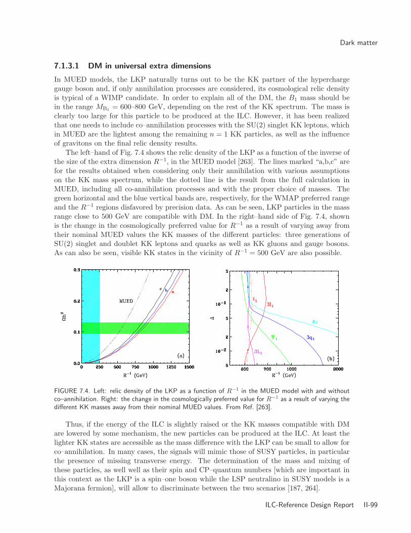
Dark matter
7.1.3.1 DM in universal extra dimensions
In MUED models, the LKP naturally turns out to be the KK partner of the hyperchargegauge boson and, if only annihilation processes are considered, its cosmological relic densityis typical of a WIMP candidate. In order to explain all of the DM, the B1 mass should bein the range MB1
= 600–800 GeV, depending on the rest of the KK spectrum. The mass isclearly too large for this particle to be produced at the ILC. However, it has been realizedthat one needs to include co–annihilation processes with the SU(2) singlet KK leptons, whichin MUED are the lightest among the remaining n = 1 KK particles, as well as the influenceof gravitons on the final relic density results.
The left–hand of Fig. 7.4 shows the relic density of the LKP as a function of the inverse ofthe size of the extra dimension R−1, in the MUED model [263]. The lines marked “a,b,c” arefor the results obtained when considering only their annihilation with various assumptionson the KK mass spectrum, while the dotted line is the result from the full calculation inMUED, including all co-annihilation processes and with the proper choice of masses. Thegreen horizontal and the blue vertical bands are, respectively, for the WMAP preferred rangeand the R−1 regions disfavored by precision data. As can be seen, LKP particles in the massrange close to 500 GeV are compatible with DM. In the right–hand side of Fig. 7.4, shownis the change in the cosmologically preferred value for R−1 as a result of varying away fromtheir nominal MUED values the KK masses of the different particles: three generations ofSU(2) singlet and doublet KK leptons and quarks as well as KK gluons and gauge bosons.As can also be seen, visible KK states in the vicinity of R−1 = 500 GeV are also possible.
FIGURE 7.4. Left: relic density of the LKP as a function of R−1 in the MUED model with and withoutco–annihilation. Right: the change in the cosmologically preferred value for R−1 as a result of varying thedifferent KK masses away from their nominal MUED values. From Ref. [263].
Thus, if the energy of the ILC is slightly raised or the KK masses compatible with DMare lowered by some mechanism, the new particles can be produced at the ILC. At least thelighter KK states are accessible as the mass difference with the LKP can be small to allow forco–annihilation. In many cases, the signals will mimic those of SUSY particles, in particularthe presence of missing transverse energy. The determination of the mass and mixing ofthese particles, as well well as their spin and CP–quantum numbers [which are important inthis context as the LKP is a spin–one boson while the LSP neutralino in SUSY models is aMajorana fermion], will allow to discriminate between the two scenarios [187, 264].
ILC-Reference Design Report II-99

CONNECTIONS TO COSMOLOGY
7.1.3.2 DM in warped extra dimensions
As discussed in chapter 6, the most promising and realistic warped extra-dimensional sce-narios need the electroweak gauge group to be extended to SU(2)L × SU(2)R × U(1)X. Inthis context, KK Dirac neutrinos charged under the SU(2)R group are necessary parts of themodels. Implementing baryon number conservation in these warped GUT models leads to aKK right–handed neutrino νR that is absolutely stable and thus, a potential candidate forcold DM [119]. In fact, even in the absence of this additional symmetry, νR can be stable atcosmological scales if the couplings involved in its decay are strongly suppressed, which canoccur also if it has a large annihilation cross section, providing the correct relic density.
In a RS scenario embedded in the SO(10) GUT group, the νR has no direct couplings tothe Z boson but a small ZνRνR coupling is induced by the mixing between the Z–Z ′ mixing.The Z ′ boson couples with full strength to the νR LKP state but, as it must be heavierthan MKK ∼ 3 TeV, the resulting interactions are rather weak. These arguments make that,although of the Dirac type, KK right–handed neutrinos with masses in the range of 1 GeVto 1 TeV can have the required relic abundance without being in conflict with the boundsfrom direct detection experiments [265]. The DM density is shown in Fig. 7.5 as a functionof the LZP mass for two values of the SO(10) coupling g10 and two different localizationsof the left–handed neutrino νL (which also mixes with νR); the masses of the KK gaugebosons are assumed to be MKK = 3, 6 and 12 TeV while the SM Higgs mass is fixed to beMH = 300 GeV. One notices the effect of the Z, Higgs and Z ′ resonances which allow for therelic density to be compatible with the WMAP range. Since all KK fermions belonging tothe multiplet containing the right–handed top quark, except for its KK mode, are expectedto be light compared to the KK gauge bosons and close in mass to the LZP, co–annihilationwith the KK leptons for instance can play a non–negligible role [265].
FIGURE 7.5. The relic density of the LZP in annihilation for three MKK values, g10 = 0.3 (dashed) and1.2 (solid lines) and two values of cνL
= 0.9 (lower) and −0.1 (upper curves); from Ref. [265].
If the LZP and the KK fermions which are in the same multiplet have not too largemasses, the ILC will be the ideal instrument to produce them and to study in great detailtheir properties. Again, threshold scans would allow for precise mass measurements and thestudy of the cross sections as well as various production and decay distributions would allowfor the determination of the couplings and spins of the particles. These measurements couldbe then used to predict the DM density and compare it with the experimental value.
II-100 ILC-Reference Design Report

The baryon asymmetry
7.2 THE BARYON ASYMMETRY
7.2.1 Electroweak baryogenesis in the MSSM
Electroweak baryogenesis is an interesting possibility where the baryon asymmetry of theuniverse is generated at the electroweak phase transition. Since the relevant energy scale isthe weak scale, this scenario has potential impacts on the Terascale physics. As a strongfirst–order phase transition is a necessary condition of successful electroweak baryogenesis,the Higgs sector should be extended from the minimal one Higgs doublet SM in which, in viewof the current bound on the Higgs boson mass, it is not the case. A strong first–order phasetransition is possible in various extensions of the Higgs sector such as the SM supplementedwith a scalar singlet field, the two Higgs doublet model, the MSSM and the next-to-minimalsupersymmetric Standard Model (NMSSM).
The electroweak baryogenesis scenario in the MSSM has been studied in detail in theliterature; see Refs. [266] for reviews. In order to account for the observed amount of baryonasymmetry, a rather specific choice of SUSY parameters is required. First, one of the topsquarks, mostly right–handed, has to be lighter than the top quark in order that a strongfirst–order phase transition is realized. The mass of the other stop, on the other hand,becomes larger than 1 TeV. A new source of CP violation necessary for the generation of thebaryon asymmetry is provided by the CP phases of the chargino and neutralino mass matrices.Since the new phases contribute to the electron and neutron electric dipole moments, scalarfermions of the first and second generations should be heaver than a few TeV, while charginosand neutralinos can be in the few 100 GeV range. Finally, the lightest Higgs boson massis predicted to be close to the present experimental bound, MH ∼ 114 GeV. If the lightestneutralino is to account for the DM in this scenario, the mass difference between the light stopand the LSP should not be large, and stop–neutralino co–annihilation [254] is the primarymechanism which generates an LSP relic abundance which matches the WMAP value.
These features are important to test this scenario at the LHC and ILC [267, 255]. Thediscovery of a light top squark and a SM–like Higgs boson with a mass close to 120 GeVwould be a strong indication that electroweak baryogenesis is the mechanism for the gen-eration of the baryon asymmetry. In order to confirm this picture, one needs to determinethat t1 is mainly right-handed and check that the masses and compositions of the charginosand neutralinos are compatible with the required values and finally, compute the DM therelic abundance so as to compare with cosmological observations. If t–χ0
1 co–annihilation isrelevant, it is important to determine the stop–neutralino mass difference very precisely. Adetailed analysis of the stop, chargino and neutralino sectors at the ILC has been performedfor this scenario in Ref. [255]. It is found that the experimental accuracies in the measure-ments of the stop and ino parameters, as discussed in chapter 5, allow to determine thestrength of the phase transition with a reasonable precision, ∆exp [v(Tc)/Tc] <∼ 10%, if thetheoretical error is ignored. The second crucial ingredient for electroweak baryogenesis, theCP–violating source responsible for the baryon asymmetry, remains however unconstrainedas only an upper bound on the phase of the µ parameter, |φµ| <∼ 0.7, can be derived.
In addition, the collider measurements can be used to predict rather precisely the DMrelic density. By determining the stop and lightest neutralino masses and the stop mixingparameters, the stop–neutralino co–annihilation cross section can be strongly constrained andthe DM relic density predicted with a precision of the same order as current astrophysicalresults. This is exemplified in Fig. 7.6 which shows the accuracy in the determination of the
ILC-Reference Design Report II-101

CONNECTIONS TO COSMOLOGY
DM abundance as a function of the stop mass in the electroweak baryogenesis scenario ofRef. [255]. While an experimental error ∆mt1
= 1.2 GeV (grey dots) leads to a relativelyloose constraint, a precision ∆mt1
= 0.3 GeV (dark dots) matches the original scenario usedas input (the red star) and the 1σ and 2σ WMAP constraints (horizontal shaded bands).Refinements in the determination of the stop mass can thus improve this result significantly.
121 122 123 124
0.08
0.1
0.12
0.14
121 122 123 124
0.08
0.1
0.12
0.14
ΩC
DM
h2
ΩC
DM
h2
mt1mt1
FIGURE 7.6. The DM abundance Ωχh2 as a function of the stop mass for the electroweak baryogenesisscenario, taking into account experimental errors for stop, ino and Higgs measurements at the ILC; thedots correspond to a scan over the 1σ region allowed by these errors; from Ref. [255].
In non–SUSY scenarios, a strong first–order electroweak phase transition needed to gen-erate the baryon asymmetry can also be made possible. For instance, this phase transitioncan be induced if the SM effective theory with one Higgs doublet Φ is augmented with adimension–six Higgs operator [111], leading to a scalar Higgs potential of the form
V = λ(Φ†Φ − 12v2)2 + 1
Λ2 (Φ†Φ − 12v2)3.
This additional term can be generated by strong dynamics at the TeV scale or by inte-grating out heavy particles such as an additional singlet scalar field [268] or the heavier Higgsparticles of a general two–Higgs doublet model [112].
At zero–temperature, the CP–even Higgs state can be expanded in terms of its usualvev, 〈ϕ〉 = v0 ' 246 GeV and the physical Higgs boson field Φ = ϕ/
√2 = (H + v0)/
√2.
From the requirement that the phase transition is first order and that the minimum at zero–temperature is a global minimum, one obtains, respectively, an upper and a lower boundon the cut–off Λ for a given Higgs mass. For a low cut–off scale, Λ <∼ 1 TeV, the requiredelectroweak phase transition can be achieved for Higgs masses MH >∼ 114 GeV [111].
As a concrete example of a possible origin of the dimension–six operator, one can have ascalar singlet N coupled to the Higgs field via an interaction of the form ζ2Φ†ΦN2. If thesinglet field has a mass mN that is larger than the weak scale, it can be integrated out andgives rise to the additional Higgs interactions, ∆V ∝ ζ2/m2
N ·|Φ|6. The baryogenesis conditionof the non–erasure of the generated baryon asymmetry is R = 〈vTc〉/Tc >∼ 1 where Tc is thecritical temperature at which the origin and the non-trivial minimum at 〈v(Tc)〉 becomedegenerate. The dependence of this ratio on the parameter ζ in the Φ†ΦN2 interaction isdisplayed in Fig. 7.7 for several values of the Higgs mass MH . As can be seen, R values largerthan unity can be obtained for Higgs masses as large as MH ∼ 200 GeV.
II-102 ILC-Reference Design Report

The baryon asymmetry
Since the Higgs potential is altered by the dimension–six operator with a low–scale cutoff,large shifts in the Higgs boson self–couplings from their SM values are generated. For instance,the trilinear Higgs coupling becomes λHHH ≡ µ = 3M2
H/v0+6v30/Λ
2 and the SM value µSM isrecovered only for Λ → ∞. In Fig. 7.7, the deviation of the trilinear Higgs coupling normalizedto its SM value, µ/µSM−1, is displayed in the [MH ,Λ] plane and one sees that shifts of orderunity can be obtained. This is particularly true in the allowed regions (delimited by thedashed lines) for the cut–off scale and the Higgs mass.
0.7 0.8 0.9 1 1.1 1.2 1.3 1.4 1.51
2
3
4
5
6
7
ζ
R
M = 100 GeVh
125
175
150
200
FIGURE 7.7. Left: the ratio R ≡ 〈v(Tc)〉/Tc as a function of the parameter ζ for several MH values [268].Right: contours of constant µ/µSM−1 in the Λ vs. MH plane; the dashed lines delimit the region in whichelectroweak baryogenesis can take place [111].
Thus, if the electroweak phase transition plays an important role for the generation of thebaryon asymmetry of the universe, there is a possibility to test this mechanism in colliderexperiments and, in particular, at the ILC. A first hint may be obtained in Higgs physicsas the nature of the electroweak phase transition is closely related to the structure of theHiggs potential and, as illustrated above, large deviations of the Higgs self–couplings fromtheir SM values are expected in this case. Another important ingredient is the new source ofCP violation that triggers the separation of particles and anti-particles during the first–orderphase transition. Since the new CP phases are carried by states that are present at thephase transition temperature, that is in the range the electroweak symmetry breaking scale,some of these particles are very likely to be within the kinematical reach of the ILC. Precisedetermination of particle masses, couplings and CP phases at the ILC will be thus essentialto confirm or disprove the electroweak baryogenesis scenario.
7.2.2 Leptogenesis and right–handed neutrinos
If leptogenesis [269] is the origin of the observed baryon asymmetry in the universe, the rootsof this phenomenon are located near the GUT or the Planck scale. CP–violating decays ofheavy right–handed Majorana neutrinos generate a lepton asymmetry which is transferred tothe quark/baryon sector by sphaleron processes. Heavy neutrino mass scales as introducedin the seesaw mechanism [211] for generating light neutrino masses and the size of the lightneutrino masses needed for leptogenesis define a self–consistent frame which is compatiblewith all experimental observations [270].
ILC-Reference Design Report II-103
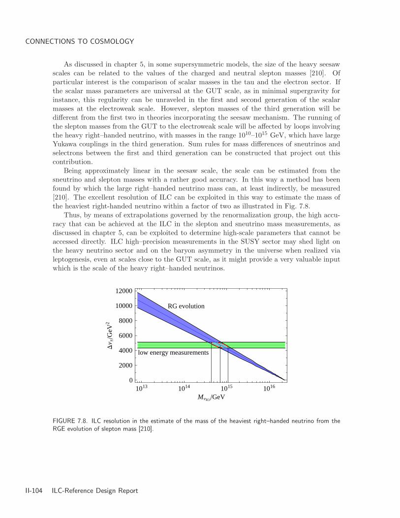
CONNECTIONS TO COSMOLOGY
As discussed in chapter 5, in some supersymmetric models, the size of the heavy seesawscales can be related to the values of the charged and neutral slepton masses [210]. Ofparticular interest is the comparison of scalar masses in the tau and the electron sector. Ifthe scalar mass parameters are universal at the GUT scale, as in minimal supergravity forinstance, this regularity can be unraveled in the first and second generation of the scalarmasses at the electroweak scale. However, slepton masses of the third generation will bedifferent from the first two in theories incorporating the seesaw mechanism. The running ofthe slepton masses from the GUT to the electroweak scale will be affected by loops involvingthe heavy right–handed neutrino, with masses in the range 1010–1015 GeV, which have largeYukawa couplings in the third generation. Sum rules for mass differences of sneutrinos andselectrons between the first and third generation can be constructed that project out thiscontribution.
Being approximately linear in the seesaw scale, the scale can be estimated from thesneutrino and slepton masses with a rather good accuracy. In this way a method has beenfound by which the large right–handed neutrino mass can, at least indirectly, be measured[210]. The excellent resolution of ILC can be exploited in this way to estimate the mass ofthe heaviest right-handed neutrino within a factor of two as illustrated in Fig. 7.8.
Thus, by means of extrapolations governed by the renormalization group, the high accu-racy that can be achieved at the ILC in the slepton and sneutrino mass measurements, asdiscussed in chapter 5, can be exploited to determine high-scale parameters that cannot beaccessed directly. ILC high–precision measurements in the SUSY sector may shed light onthe heavy neutrino sector and on the baryon asymmetry in the universe when realized vialeptogenesis, even at scales close to the GUT scale, as it might provide a very valuable inputwhich is the scale of the heavy right–handed neutrinos.
1013 1014 1015 1016
MΝR3GeV
0
2000
4000
6000
8000
10000
12000
DΝΤG
eV2
low energy measurements
RG evolution
FIGURE 7.8. ILC resolution in the estimate of the mass of the heaviest right–handed neutrino from theRGE evolution of slepton mass [210].
II-104 ILC-Reference Design Report

BIBLIOGRAPHY
[1] A. Albrecht et al., report of the DOE/NSF High Energy Physics Advisory Panel (2004).
[2] H. Shapiro et al., “Revealing the hidden nature of space and time: charting thecourse for elementary particle physics”, report of the Committee on Elementary Parti-cle Physics in the 21st Century, Board of Physics and Astronomy, National ResearchCouncil, National Academies Press, Washington D.C. (2006).
[3] “The European Strategy for Particle Physics”, Report of CERN Council StrategyGroup (2006).
[4] GLC project: Linear collider for TeV physics, KEK-REPORT-2003-7.
[5] I. Corbett et al., Report of the Consultative Group on High-Energy Physics, OECDGlobal Science Forum (2002).
[6] S. Yamada et al., Report of the JLC Globalization Committee (2002).
[7] ECFA/DESY LC Physics WG, J. A. Aguilar-Saavedra et al., hep-ph/0106315.
[8] ACFA Linear Collider Working Group, K. Abe et al., hep-ph/0109166.
[9] American Linear Collider Working Group, T. Abe et al., hep-ex/0106057.
[10] ECFA/DESY LC Physics Working Group, E. Accomando et al., Phys. Rept. 299, 1(1998), [hep-ph/9705442].
[11] J. Bagger et al., “Discovering the Quantum Universe: The role of particle colliders,”report of the DOE/NSF High Energy Physics Advisory Panel (2006).
[12] ATLAS Collaboration, Physics TDR, CERN-LHCC-99-14 and CERN-LHCC-99-15.
[13] CMS Collaboration, Physics TDR, CERN/LHCC/2006-021, June 2006.
[14] R. Cousins, J. Mumford and V. Valuev, CERN-CMS-NOTE-2005-022.
[15] LHC/LC Study Group, G. Weiglein et al., Phys. Rept. 426, 47 (2006).
[16] Parameters for the Linear Collider,http://www.fnal.gov/directorate/icfa/LC_parameters.pdf.
[17] G. A. Moortgat-Pick et al., hep-ph/0507011.
[18] P. D. Grannis, hep-ex/0211002.
ILC-Reference Design Report II-105

BIBLIOGRAPHY
[19] R. Hawkings and K. Monig, Eur. Phys. J. direct C1, 8 (1999).
[20] C. A. Heusch, Int. J. Mod. Phys. A20, 7289 (2005).
[21] I. F. Ginzburg, G. L. Kotkin, V. G. Serbo and V. I. Telnov, JETP Lett. 34, 491 (1981).
[22] ECFA/DESY Photon Collider Working Group, B. Badelek et al., hep-ex/0108012.
[23] F. Bechtel et al., Nucl. Instrum. Meth. A564, 243 (2006).
[24] S. Dawson and M. Oreglia, Ann. Rev. Nucl. Part. Sci. 54, 269 (2004).
[25] M. Battaglia et al., hep-ex/0603010.
[26] For a review on ILC physics scenarios: W. Kilian and P. Zerwas, hep-ph/0601217.
[27] T. Barklow, talk at ILCWS, 2005, Stanford, California.
[28] S. Hillert, Talk at ILC Software and Physics Meeting, 4-6 April 2006, Cambridge, UK.
[29] T. Behnke et al., TESLA TDR part 4: A detector for TESLA, DESY-01-011.
[30] M. A. Thomson, physics/0607261.
[31] P.W. Higgs, Phys. Rev. Lett. 13, 508 (1964) and Phys. Rev. 145,1156 (1966); F.Englert and R. Brout, Phys. Rev. Lett. 13, 321 (1964); G.S. Guralnik, C.R. Hagen andT. Kibble, Phys. Rev. Lett. 13, 585 (1965).
[32] J. Gunion, H. Haber, G. Kane, and S. Dawson, The Higgs Hunters Guide, Addison–Wesley, Reading (USA), 1990. See also, M. Gomez-Bock et al., hep-ph/0509077.
[33] A. Djouadi, hep-ph/0503172, to appear in Phys. Rept.
[34] LEP WG for Higgs boson searches, R. Barate et al., Phys. Lett. B565, 61 (2003).
[35] The particle Data Group, J.-W. Yao et al., J. Phys. G33, 1 (2006).
[36] The LEP collaborations and the LEP electroweak working group, hep-ex/0612034.
[37] T. Hambye and K. Riesselmann, Phys. Rev. D55, 7255 (1997).
[38] B.W. Lee, C. Quigg and H.B. Thacker, Phys. Rev. D16, 1519 (1977).
[39] M. Luscher and P. Weisz, Phys. Lett. B212, 472 (1988); M. Gockeler, H. Kastrup, T.Neuhaus and F. Zimmermann, Nucl. Phys. B405, 555 (1993).
[40] A. Djouadi, hep-ph/0503173, to appear in Phys. Rept.
[41] S. Heinemeyer, W. Hollik and G. Weiglein, Phys. Rept. 425, 265 (2006).
[42] The LEP Collaboration (ALEPH, DELPHI, L3, OPAL), Eur. Phys. J. C47, 547 (2006).
[43] For a recent review, see E. Accomando et al., hep-ph/0608079.
[44] M. Carena, J. R. Ellis, A. Pilaftsis and C. E. Wagner, Nucl. Phys. B 625, 345 (2002).
II-106 ILC-Reference Design Report

BIBLIOGRAPHY
[45] M. Carena, J. R. Ellis, A. Pilaftsis and C. E. Wagner, Nucl. Phys. B 659, 145 (2003).
[46] S.Y. Choi, J. Kalinowski, Y. Liao and P.M. Zerwas, Eur. Phys. J. C40, 55 (2005).
[47] D. J. Miller, R. Nevzorov and P. M. Zerwas, Nucl. Phys. B681, 3 (2004).
[48] See e.g., J. Espinosa and M. Quiros, Phys. Rev. Lett. 81, 516 (1998).
[49] See e.g.: U.Ellwanger, C.Hugonie and J.Gunion, JHEP 0502, 066 (2005).
[50] For recent analyses, see: U. Ellwanger and C. Hugonie, Eur. Phys. J. C25, 297 (2002);U. Ellwanger et al., hep-ph/0111179 and hep-ph/0305109; J. Gunion and R. Dermisek,Phys. Rev. Lett. 95, 041801 (2005); V. Barger et al., Phys. Rev. D73, 115010 (2006).
[51] See e.g. S. King, S. Moretti and R. Nevzorov, Phys. Rev. D73, 035009 (2006).
[52] See e.g. T. Han, P. Langacker and B. McElrath, Phys. Rev. D70, 115006 (2004).
[53] For a review, see for instance: J. Gunion, hep-ph/0212150.
[54] M. Hirsch, J. Romao, J. Valle and A. Villanova del Moral, Phys. Rev. D73, 055007(2006); A. Villanova del Moral in Ref. [43].
[55] L. Randall and R. Sundrum, Phys. Rev. Lett. 83, 3370 (1999).
[56] J. L. Hewett and T. G. Rizzo, JHEP 08, 028 (2003).
[57] D. Dominici, B. Grzadkowski, J. Gunion and M. Toharia, Nucl. Phys. B671, 243(2003).
[58] N. Arkani-Hamed, S. Dimopoulos and G. Dvali, Phys. Lett. B429, 263 (1998) andPhys. Rev. D59, 086004 (1999); A. Antoniadis, N. Arkani-Hamed, S. Dimopoulos andG. Dvali, Phys. Lett. B436, 267 (1998).
[59] G. Giudice, R. Rattazi and J. Wells, Nucl. Phys. 595, 250 (2001); M. Battaglia, D.Dominici, J. Gunion and J. Wells, hep-ph/0402062.
[60] J. van der Bij, Phys. Lett. B636, 56 (2006); S. Dilcher and J. van der Bij, Phys. Lett.B638, 234 (2006); see also, J. Kumar and J.D. Wells, Phys. Rev. D74, 115017 (2006).
[61] N. Arkani-Hamed et al., JHEP 08, 021 (2002); N. Arkani-Hamed, A. Cohen, E. Katz,and A. Nelson, JHEP 07, 034 (2002).
[62] S. Weinberg, Phys. Rev. D13, 974 (1979) and Phys. Rev. D19, 1277 (1979); L.Susskind, Phys. Rev. D20, 2619 (1979).
[63] For a review on strong EWSB: C. Hill and E. Simmons, Phys. Rept. 381 (2003) 235.
[64] W. Kilian, D. Rainwater and J. Reuter, Phys. Rev. D74, 095003 (2006) [Erratum-ibid.D74, 099905 (2006) and Phys. Rev. D71, 015008 (2005).
[65] G. Giudice, C. Grojean, A. Pomarol and R. Rattazzi, hep-ph/0703164.
[66] C. Csaki et al., Phys. Rev. D69, 055006 (2004); C. Csaki, C. Grojean, L. Pilo and J.Terning, Phys. Rev. Lett. 92, 101802 (2004).
ILC-Reference Design Report II-107
BIBLIOGRAPHY
[67] M. Duhrssen et al., Phys. Rev. D70, 113009 (2004).
[68] E.Boos et al., Phys. Rev. D66, 055004 (2002); Phys. Lett. B578, 384 (2004) and Phys.Lett. B622, 311 (2005).
[69] A. Djouadi, J. Kalinowski and M. Spira, Comput. Phys. Commun. 108, 56 (1998).
[70] A. Djouadi, M. Spira and P. M. Zerwas, Z. Phys. C70, 427 (1996); A. Djouadi, J. Kali-nowski and P. M. Zerwas, Z. Phys. C70, 435 (1996); M. Spira et al., Phys. Lett. B264,440 (1991) and Nucl. Phys. B453, 17 (1995).
[71] J. Ellis, M.K. Gaillard and D.V. Nanopoulos, Nucl. Phys. B106, 292 (1976); J.D.Bjorken, SLAC Report 198 (1976); B. Ioffe and V.A. Khoze, Sov. J. Part. Nucl. 9, 50(1978); D.R.T. Jones and S.T. Petcov, Phys. Lett. B84, 440 (1979).
[72] R.N. Cahn and S. Dawson, Phys. Lett. B136, 196 (1984); K. Hikasa, Phys. Lett.164B, 385 (1985); G. Altarelli, B. Mele and F. Pitolli, Nucl. Phys. B287, 205 (1987);W. Kilian, M. Kramer and P.M. Zerwas, Phys. Lett. B373, 135 (1996).
[73] K. Gaemers and G. Gounaris, Phys. Lett. B77, 379 (1978); A. Djouadi, J. Kalinowskiand P. M. Zerwas, Z. Phys. C54, 255 (1992) and Mod. Phys. Lett. A7, 1765 (1992).
[74] G. Gounaris, D. Schildknecht and F.M. Renard. Phys. Lett. B83, 191 (1979); V. Bargeret al., Phys. Rev. D49, 79 (1994); A. Djouadi, H.E. Haber and P.M. Zerwas, Phys. Lett.B375, 203 (1996); V.A. Ilyin et al., Phys. Rev. D54, 6717 (1996).
[75] A. Djouadi, W. Kilian, M. Muhlleitner and P. Zerwas, Eur. Phys. J. C10, 27 (1999).
[76] S. Dittmaier et al., Phys. Lett. B441, 383 (1998) and Phys. Lett. B478, 247 (2000);A. Denner et al., Nucl. Phys. B680, 85 (2004); G. Belanger et al., Phys. Lett. B571,163 (2003); Y. You et al., Phys. Lett. B571, 85 (2003).
[77] C. Farrell and A. H. Hoang, Phys. Rev. D74, 014008 (2006).
[78] G. Belanger et al., Phys. Lett. B576, 152 (2003); T. Zhang et al., Phys. Lett. B578,349 (2004); Y. Yasue et al., talk at ECFA Workshop, Durham, Sept. 2004.
[79] P. Niezurawski, A.F. Zarnecki and M. Krawczyk, JHEP 0502, 041 (2005).
[80] P. Bambade and F. Richard, hep-ph/0703173.
[81] K. Desch et al., Report of the Higgs WG for the extended ECFA-DESY study, Ams-terdam, 2003, hep-ph/0311092.
[82] P. Garcia-Abia and W. Lohmann, Eur. Phys. J. direct C2, 2 (2000).
[83] P. Garcia-Abia, W. Lohmann and A. Raspereza, hep-ex/0505096.
[84] D.J. Miller et al., Phys. Lett. B505, 149 (2001).
[85] V. Barger et al., Phys. Rev. D49, 79 (1994).
[86] M. T. Dova, P. Garcia-Abia and W. Lohmann, hep-ph/0302113.
II-108 ILC-Reference Design Report

BIBLIOGRAPHY
[87] M. Schumacher, LC-PHSM-2001-003.
[88] M. Kramer, J. H. Kuhn, M. L. Stong and P. M. Zerwas, Z. Phys. C64, 21 (1994).
[89] B. Grzadkowski, J. Gunion and X. He, Phys. Rev. Lett. 77, 5172 (1996); P.S. BhupalDev et al., arxiv:0707.2878 [hep-ph].
[90] N. Meyer and K. Desch, Eur. Phys. J. C35, 171 (2004).
[91] M. D. Hildreth, Talk at High-Energy Physics with Colliding Beams, Santa Cruz, 1992.
[92] M. Schumacher, LC-PHSM-2003-096.
[93] M. Battaglia, hep-ph/9910271.
[94] J. C. Brient, LC-PHSM-2002-003.
[95] G. Borisov and F. Richard, hep-ph/9905413.
[96] E. Boos et al., Eur. Phys. J. C19, 455 (2001).
[97] T. Kuhl and K. Desch, LC-PHSM-2007-2.
[98] M. Battaglia, hep-ph/0211461.
[99] T. Barklow, hep-ph/0312268.
[100] A. Juste and G. Merino, hep-ph/9910301; K. Desch and M. Schmucher in [15]; S.Dawson, A. Juste, L. Reina and D. Wackeroth in [15].
[101] A. Gay, Eur. Phys. J. C49, 489 (2007).
[102] A. Juste, hep-ph/0512246.
[103] K. Hagiwara, H. Murayama and I. Watanabe, Nucl. Phys. B367, 257 (1991), S. Bar-Shalom, D. Atwood and A. Soni, Phys. Lett. B419, 340 (1998); B. Grzadkowski andJ. Pliszka, Phys. Rev. D60, 115018 (1999).
[104] J. Alcaraz and E. Ruiz Morales, Phys. Rev. Lett. 86, 3726 (2001).
[105] C. Castanier, P. Gay, P. Lutz and J. Orloff, hep-ex/0101028.
[106] U. Baur, T. Plehn and D. Rainwater in [15].
[107] M. Battaglia, E. Boos and W.-M. Yao, hep-ph/0111276.
[108] Y. Yasui et al., hep-ph/0211047.
[109] S. Yamashita, talk at LCWS04, Paris. April 2004.
[110] P. Niezurawski, A. F. Zarnecki and M. Krawczyk, hep-ph/0307183.
[111] C. Grojean, G. Servant and J. Wells, Phys. Rev. D71, 036001 (2005).
[112] S. Kanemura, Y. Okada and E. Senaha, Phys. Lett. B606, 361 (2005).
ILC-Reference Design Report II-109

BIBLIOGRAPHY
[113] A. Djouadi, Phys. Lett. B435, 101 (1998); A. Djouadi and G. Moreau, arXiv:0707.3800[hep-ph].
[114] J.F. Gunion et al., Phys. Rev. D38, 3444 (1988); A. Brignole et al., Report DESY-92-123B; A. Djouadi, J. Kalinowski and P.M. Zerwas, Z. Phys. C57, 569 (1993) and Z.Phys. C74, 93 (1997).
[115] S. Kiyoura et al., hep-ph/0301172.
[116] J.F. Gunion and H.E. Haber, Phys. Rev. D48, 5109 (1993); M.M. Muhlleitner et al.,Phys. Lett. B508, 311 (2001).
[117] D. Asner, J. Gronberg and J. Gunion, Phys. Rev. D67, 035009 (2003).
[118] K. Desch, T. Klimkovich, T. Kuhl and A. Raspereza, hep-ph/0406229.
[119] K. Agashe and G. Servant, Phys. Rev. Lett. 93, 231805 (2004) and JCAP 0502, 002(2005); D. Hooper and G. Servant, Astropart. Phys. 24, 231 (2005).
[120] The ALEPH, DELPHI, L3, OPAL, SLD Collaborations, the LEP Electroweak WorkingGroup, the SLD Electroweak and Heavy Flavour Groups, Phys. Rept. 427, 257 (2006).
[121] The LEP collaborations and the LEP electroweak working group, CERN-PPE/93-157.
[122] S. Riemann, LC-TH-2001-007.
[123] F. Jegerlehner, Nucl. Phys. Proc. Suppl. 162, 22 (2006), [hep-ph/0608329].
[124] A. Djouadi, G. Moreau and F. Richard, Nucl. Phys. B773, 43 (2007).
[125] G. Wilson, LC-PHSM-2001-009.
[126] J.F. Gaemers and G. Gounaris, Zeit. Phys. C1, 259 (1979); K. Hagiwara, R. Peccei, D.Zeppenfeld and K. Hikasa, Nucl. Phys. B282, 253 (1987).
[127] W. Menges, LC-PHSM-2001-022.
[128] K. Monig and J. Sekaric, Eur. Phys. J. C38, 427 (2005), [hep-ex/0410011].
[129] K. Monig and J. Sekaric, hep-ex/0507050.
[130] T. Appelquist and C. Bernard, Phys. Rev. D22, 200 (1980); A. Longhitano, Phys.Rev. D22, 1166 (1980) and Nucl. Phys. B188, 118 (1981); T. Appelquist and G.H.Wu, Phys. Rev. D48, 3235 (1993).
[131] M. Beyer et al., Eur. Phys. J. C48, 353 (2006), [hep-ph/0604048].
[132] O. Biebel, hep-ex/9912051.
[133] M. Winter, PHSM-2001-016.
[134] B.C. Allanach et al., hep-ph/0403133 and Nucl. Phys. Proc.Suppl. 135, 107 (2004).
[135] E. De Pree and M. Sher, Phys. Rev. D73, 095006 (2006).
II-110 ILC-Reference Design Report
BIBLIOGRAPHY
[136] R. Chivukula, S. Selipsky and E. Simmons, Phys. Rev. Lett. 69, 575 (1992); R.Chivukula, E. Simmons and J. Terning, Phys. Lett. B331, 383 (1994); K. Hagiwaraand N. Kitazawa, Phys. Rev. D52, 5374 (1995); U. Mahanta, Phys. Rev. D55, 5848(1996).
[137] M. Jezabek, T. Nagano and Y. Sumino, Phys. Rev. D62, 014034 (2000).
[138] S. Heinemeyer, S. Kraml, W. Porod and G. Weiglein, JHEP 09, 075 (2003).
[139] M. E. Peskin and J. D. Wells, Phys. Rev. D64, 093003 (2001).
[140] K. Fujii, T. Matsui and Y. Sumino, Phys. Rev. D50, 4341 (1994).
[141] M. Martinez and R. Miquel, Eur. Phys. Jour. C27, 49 (2003).
[142] A. H. Hoang and T. Teubner, Phys. Rev. D60, 114027 (1999); A. H. Hoang, Z. Ligetiand A. V. Manohar, Phys. Rev. Lett. 82, 277 (1999).
[143] A. H. Hoang, Phys. Rev. D69, 034009 (2004).
[144] A. H. Hoang and I. W. Stewart, Phys. Rev. D67, 114020 (2003).
[145] K. G. Chetyrkin and M. Steinhauser, Nucl. Phys. B573, 617 (2000); A. Hoang et al.,Eur. Phys. J. direct C2, 1 (2000).
[146] S. Boogert and D.J. Miller, hep-ex/0211021; A. Hinze and K. Monig, physics/0506115.
[147] K. Monig, LC-PHSM-2000-060.
[148] S. T. Boogert in a talk at Snowmass 2005.
[149] S. Moretti, hep-ph/9911501.
[150] W. Hollik et al., Nucl. Phys. B551, 3 (1999).
[151] B. Grzadkowski and Z. Hioki, Nucl. Phys. B585, 3 (2000).
[152] S.D. Rindani, Pramana 61, 33 (2003) and Pramana 54, 791 (2000).
[153] B. Grzadkowski and Z. Hioki, Phys. Lett. B476, 87 (2000); ibid. 557, 55 (2003).
[154] W. Bernreuther, talk given at the ECFA/DESY LCWS, Oxford, UK, March 1999.
[155] M. Beneke et al., hep-ph/0003033.
[156] P. Batra and T. M. P. Tait, Phys. Rev. D74, 054021 (2006).
[157] J. A. Aguilar-Saavedra and T. Riemann, hep-ph/0102197.
[158] J.-J. Cao, Z.-H. Xiong and J. M. Yang, Nucl. Phys. B651, 87 (2003).
[159] A. Brandenburg, Eur. Phys. J. C11, 127 (1999) and LC-TH-1999-009.
[160] T. Rizzo, Phys. Rev. D50, 4478 (1994); R. Martinez et al., hep-ph/9709478.
[161] V.A. Khoze, W.J. Stirling and L.H. Orr, Nucl. Phys. B378, 413 (1992).
ILC-Reference Design Report II-111

BIBLIOGRAPHY
[162] V.A. Khoze and T. Sjostrand, Eur. Phys. J. direct C2, 1 (2000).
[163] A. Brandenburg, L. Dixon and Y. Shadmi, Phys. Rev. D53, 1264 (1996).
[164] G.A. Blair, in DESY 97-123E; G.A. Blair et al., in DESY 1997-048.
[165] J. Wess and B. Zumino, Nucl. Phys. B70, 39 (1974); Yu. A. Gol’fand and E. P. Likht-man, JETP Lett. 13, 323 (1971).
[166] For a review, see: J. Wess and J. Bagger, “Supersymmetry and Supergravity”, Prince-ton Series in Physics, New Jersey, 1992.
[167] E. Witten, Nucl. Phys. B188, 513 (1981) and Nucl. Phys. B202, 253 (1982).
[168] L. Ibanez and G. Ross, Phys. Lett. B110, 227 (1982); L. Alvarez–Gaume, J. Polchinskiand M. Wise, Nucl. Phys. B221, 495 (1983); J. Ellis et al., Phys. Lett. B125, 275(1983); L. Ibanez, C. Lopez and C. Munoz, Nucl. Phys. B256, 218 (1985).
[169] W. J. Marciano and G. Senjanovic, Phys. Rev. D25, 3092 (1982); J. Ellis, S. Kelleyand D. Nanopoulos, Phys. Lett. B260, 131 (1991); U. Amaldi, W. de Boer and H.Furstenau, Phys. Lett. B260 447, (1991); P. Langacker and M. Luo, Phys. Rev. D44,817 (1991); C. Giunti, C. Kim and U. Lee, Mod. Phys. Lett. A6, 1745 (1991).
[170] G.R. Farrar and P. Fayet, Phys. Lett. B76, 575 (1978).
[171] H. Goldberg, Phys. Rev. Lett. 50, 1419 (1983); J. Ellis et al., Nucl. Phys. B238, 453(1984).
[172] For reviews, see: G. Jungman, M. Kamionkowski and K. Griest, Phys. Rept. 267, 195(1996); G. Bertone, D. Hooper and J. Silk, Phys. Rept. 405, 279 (2005); M. Drees,hep-ph/0509105; J. Feng, hep-ph/0509309; K. Olive, hep-ph/0412054.
[173] For reviews, see: H.P. Nilles, Phys. Rept. 110, 1 (1984); H. Haber and G. Kane, Phys.Rept. 117, 75 (1985); S. Martin, hep-ph/9709356; M. Drees, R. Godbole and P. Roy,“Theory and Phenomenology of Sparticles”, World Scientific, 2004.
[174] A.H. Chamseddine, R. Arnowitt and P. Nath, Phys. Rev. Lett. 49, 970 (1982); R.Barbieri, S. Ferrara and C.A Savoy, Phys. Lett. B119, 343 (1982); L. Hall, J. Lykkenand S. Weinberg, Phys. Rev. D27, 2359 (1983).
[175] L. Randall and R. Sundrum, Nucl. Phys. B557, 79 (1999); G. Giudice, M. Luty, H.Murayama and R. Rattazzi, JHEP 9812, 027 (1998); J.A. Bagger, T. Moroi and E.Poppitz, JHEP 0004, 009 (2000).
[176] For a review, see: G.F. Giudice and R. Rattazzi, Phys. Rept. 322, 419 (1999).
[177] J.R. Ellis, J.E. Kim and D.V. Nanopoulos, Phys. Lett. B145, 181 (1984); T. Moroi, H.Murayama and M. Yamaguchi, Phys. Lett. B303, 289 (1993).
[178] For reviews, see: H. Dreiner, hep-ph/9707435; G. Barbier et al., hep-ph/9810232.
[179] J.A. Aguilar–Saavedra et al., Eur. Phys. J. C46, 43 (2006).
[180] J. Kalinowski, hep-ph/0309235.
II-112 ILC-Reference Design Report

BIBLIOGRAPHY
[181] H. Baer, ISAJET, F.E. Paige, S.D. Protopopescu and X. Tata, hep-ph/0001086. OtherRGE codes are, SuSpect: A. Djouadi, J. L. Kneur and G. Moultaka, Comput. Phys.Commun. 176, 426 (2007); Softsusy: B. Allanach, Comput. Phys. Commun. 143, 305(2002); Spheno: W. Porod, Comput. Phys. Commun. 153, 275 (2003).
[182] B. C. Allanach et al., Eur. Phys. J. direct C25, 113 (2002).
[183] M. Battaglia et al., Eur. Phys. J. C22, 535 (2001) and Eur. Phys. J. C33, 273 (2004).
[184] K. Desch et al., in Ref. [15] and JHEP 0402, 035 (2004) and hep-ph/0410121.
[185] H.U. Martyn, LC-PHSM-2003-07, hep-ph/0302024 and in Ref. [15].
[186] C. Hensel, DESY-THESIS-2002-047.
[187] S.Y. Choi, K. Hagiwara, H. Martyn, K. Mawatari and P. Zerwas, hep-ph/0612301.
[188] M. Berggren, F. Richard, and Z. Zhang, hep-ph/0510088.
[189] K. Desch et al., JHEP 0612, 007 (2006).
[190] See for instance, A. Bartl, S. Hesselbach, K. Hidaka, T. Kernreiter and W. Porod, Phys.Rev. D70, 035003 (2004); S. Hesselbach, Acta. Phys. Pol. B35, 2739 (2004).
[191] A. Freitas, D. J. Miller and P. M. Zerwas, Eur. Phys. J. C21, 361 (2001); A. Freitas,A. von Manteuffel, P.M. Zerwas Eur. Phys. J. C34, 487 (2004).
[192] A. Freitas, U. Martyn, U. Nauenberg and P.M. Zerwas, hep-ph/0409129.
[193] M. Nojiri, Phys. Rev. D51, 6281 (1995); M. Nojiri, K. Fujii and T. Tsukamoto, Phys.Rev. D54, 6756 (1996).
[194] E. Boos et al., hep-ph/0211040 and hep-ph/0303110.
[195] L. Calibbi, Y. Mambrini and S.K. Vempati, arXiv:0704.3518 [hep-ph].
[196] S.Y. Choi, H.U. Martyn and P.M. Zerwas, Eur. Phys. J. C44, 175 (2005).
[197] S.Y. Choi et al., Phys. Lett. B606, 164 (2005).
[198] J. Hisano, M. M. Nojiri, Y. Shimizu, and M. Tanaka, Phys. Rev. D60, 055008 (1999);W. Porod and W. Majerotto, Phys. Rev. D66, 015003 (2002).
[199] F. Deppisch, H. Martyn, H. Pas, A. Redelbach and R. Ruckl, hep-ph/0408140.
[200] A. Finch, H. Nowak and A. Sopczak, hep-ph/0211140, LC-PHSM-2003-075; A. Sopczaket al., talk at SUSY05, Durham.
[201] H. U. Martyn, Eur. Phys. J. C48, 15 (2006).
[202] See for instance, A. Abada, G. Bhattacharyya and M. Losada, Phys. Rev. D66, 071701(2002); F. Borzumati and J.S. Lee, Phys. Rev. D66, 115012 (2002).
[203] U. Ellwanger and C. Hugonie, Eur. Phys. J. C5, 723 (1998) and C13, 681 (2000);F. Franke and S. Hesselbach, Phys. Lett. B526, 370 (2002) and hep-ph/0210363; G.Moortgat-Pick et al., JHEP 0506, 048 (2005).
ILC-Reference Design Report II-113

BIBLIOGRAPHY
[204] S. Y. Choi, J. Kalinowski, G. Moortgat-Pick and P. M. Zerwas, Eur. Phys. J. C22, 563(2001) and addendum Eur. Phys. J. C23, 769 (2002).
[205] S. Y. Choi et al., Eur. Phys. J. C7, 123 (1999); Eur. Phys. J. C8, 669 (1999); Eur.Phys. J. C14, 535 (2000); J.L. Kneur and G. Moultaka, Phys. Rev. D59, 015005 (1999)and Phys. Rev. D61, 095003 (2000).
[206] R. Lafaye, T. Plehn and D. Zerwas, hep-ph/0404282 and hep-ph/0512028.
[207] P. Bechtle, K. Desch and P. Wienemann, Comput. Phys. Commun. 174, 47 (2006).
[208] G. A. Blair, W. Porod and P. M. Zerwas, Eur. Phys. J. C27, 263 (2003).
[209] P. Binetruy, M. K. Gaillard and B. D. Nelson, Nucl. Phys. B 604, 32 (2001).
[210] A. Freitas, W. Porod and P. M. Zerwas, Phys. Rev. D72, 115002 (2005).
[211] P. Minkowski, Phys. Lett. B67, 421 (1977); M. Gell-Mann, P. Ramond, and R. Slansky,Proceedings, Workshop Stony Brook 1979; T. Yanagida, Proceedings, Workshop KEK(Tsuhuba) 1979; R. N. Mohapatra and G. Senjanovic, Phys. Rev. Lett. 44, 912 (1980).
[212] T. Appelquist, H.-C. Cheng and B. A. Dobrescu, Phys. Rev. D64, 035002 (2001).
[213] H.C. Cheng and I. Low, JHEP 09, 051 (2003) and JHEP 08, 061 (2004); I. Low, JHEP10, 067 (2004).
[214] N. Arkani-Hamed, M. Porrati and L. Randall, JHEP 08, 017 (2001); R. Rattazzi andA. Zaffaroni, JHEP 04, 021 (2001).
[215] R. Contino, Y. Nomura and A. Pomarol, Nucl. Phys. B671, 148 (2003); K. Agashe, R.Contino and A. Pomarol, Nucl. Phys. B719, 165 (2005).
[216] L.J. Hall and D. Smith, Phys. Rev. D60, 085008 (1999); S. Cullen and M. Perelstein,Phys. Rev. Lett. 83, 268 (1999); V. Barger, T. Han and R.J. Zhang, Phys. Lett. B461,34 (1999).
[217] S. Hannestad and J. Raffelt, Phys. Rev. D67, 125008 (2003).
[218] G.W. Wilson, LC-PHSM-2001-010.
[219] T. G. Rizzo, JHEP 02, 008 (2003).
[220] T.G. Rizzo, JHEP 10, 013 (2002); N. Delerue, K. Fujii and N. Okada, Phys. Rev. D70,091701 (2004).
[221] H. Davoudiasl, J.L. Hewett and T.G. Rizzo, Phys. Rev. Lett. 84, 2080 (2000) and Phys.Rev. D63, 075004 (2001).
[222] B. C. Allanach, K. Odagiri, M. A. Parker and B. R. Webber, JHEP 09, 019 (2000).
[223] T. Gherghetta and A. Pomarol, Nucl. Phys. B586, 141 (2000).
[224] D. Hooper and S. Profumo, hep-ph/0701197.
II-114 ILC-Reference Design Report

BIBLIOGRAPHY
[225] G. Servant and T. Tait, Nucl. Phys. B650, 391 (2003); M. Kakizaki, S. Matsumoto,Y. Sato and M. Senami, Phys. Rev. D71, 123522 (2005) and Nucl. Phys. B735, 84(2006); F. Burnell and G. Kribs, Phys. Rev. D73, 015001 (2006); N. Shah, Nausheenand C. Wagner, Phys. Rev. D74, 104008 (2006).
[226] J. Conley, J. Hewett and M. Le, Phys. Rev. D72, 115014 (2005).
[227] C. Berger, M. Perelstein and F. Petriello, hep-ph/0512053.
[228] M. Schmaltz, JHEP 08, 056 (2004).
[229] T. Barklow, proceedings of the 5th ILCWS, 2000.
[230] R. Casalbuoni et al., JHEP 9908, 11 (1999) and Nucl. Phys. B555, 3 (1999).
[231] R. Casalbuoni et al., Nucl. Phys. 282, 235 (1987) and Phys. Rev. D53, 5201 (1996).
[232] For a reviedw, see: J. Lykken, Czech. J. Phys. 55, B577 (2005).
[233] A. Birkedal, K. Matchev and M. Perelstein, Phys. Rev. Lett. 94, 191803 (2005).
[234] J. Hewett and T. Rizzo, Phys. Rept. 183 (1989) 193.
[235] A. Leike, Phys. Rept. 317 (1999) 143; A. Djouadi et al., Z. Phys. C56 (1992) 289; M.Cvetic and P. Langacker, hep-ph/9707451.
[236] F. Richard, hep-ph/0303107.
[237] S. Godfrey, P. Kalyniak and A. Tomkins, hep-ph/0511335.
[238] S. Godfrey, P. Kalyniak, B. Kamal and A. Leike, Phys. Rev. D61, 113009 (2000).
[239] For a review, see: A. Djouadi, J. Ng and T.G. Rizzo et al., hep-ph/9504210.
[240] For a detailed simulation, see e.g., A. Djouadi and G. Azuelos, Z. Phys. C63, 327(1994); based on A. Djouadi, Z. Phys. C63, 317 (1994).
[241] W. Buchmuller and C. Greub, Nucl. Phys.B363, 345 (1991); M. Spira in Ref. [7].
[242] J. Hewett and T. Rizzo, Phys. Rev. D36, 3367 (1987) and Phys. Rev. D56, 5709(1997); J. Blumlein and R. Ruckl, Phys. Lett. B304 (1993); J. Blumlein, E. Boos andA. Kryukov, Phys. Lett. B392, 150 (1997).
[243] R. Ruckl, R. Settles and H. Spiesberger, in DESY 1997-048, chapter 1.8.3.
[244] T. Rizzo, Int. J. Mod. Phys. A13, 2351 (1998); J. Hewett in Ref. [239].
[245] K. Hagiwara, D. Zeppenfeld and S. Komamiya, Z. Phys. C29, 115 (1985); F. Boudjema,A. Djouadi and J. Kneur, Z. Phys. C57, 425 (1993) and Phys. Lett. B240, 485 (1990).
[246] J. Bond, G. Efstathiou and Tegmark, Mon. Not. Roy. Astron. Soc. 291, L33 (1997).
[247] A. D. Sakharov, Pisma Zh. Eksp. Teor. Fiz. 5, 32 (1967).
[248] J. Lubish and P. Meade, Phys. Rev. D71, 035016 (2005); A. Birkedal, A. Noble, M.Perelstein and A. Spray, Phys. Rev. D74, 035002 (2006).
ILC-Reference Design Report II-115
BIBLIOGRAPHY
[249] C. Hill and R. Hill, arXiv:0705.0697 [hep-ph].
[250] For studies at LHC, see e.g., M. Battaglia, I. Hinchliffe and D. Tovey, hep-ph/0406147;M. Nojiri, G. Polesello and D.R. Tovey, JHEP 0603, 063 (2006).
[251] J. Ellis, K. Olive, Y. Santoso and V.C. Spanos, Phys. Lett. B565, 176 (2003).
[252] E. Baltz, M. Battaglia, M. Peskin and T. Wizansky, Phys. Rev. D74, 103521 (2006).
[253] See e.g.: H. Baer et al., JHEP 0402, 007 (2004) and JHEP 406, 061 (2004); A. Djouadi,M. Drees and J.L. Kneur, Phys. Lett. B624, 60 (2005) and JHEP 0603, 033 (2006).
[254] C. Bohm, A. Djouadi and M. Drees, Phys. Rev. D62, 035012 (2000); R. Arnowitt, B.Dutta and Y. Santoso, Nucl. Phys. B606, 59 (2001); J.R. Ellis, K.A. Olive and Y.Santoso, Astropart. Phys. 18, 395 (2003).
[255] M. Carena et al., Phys. Rev. D72, 115008 (2005); M. Carena, and A. Freitas, Phys.Rev. D74, 095004 (2006).
[256] The figure is originally from J.L. Feng, J. Phys. G32, R1 (2006). It has been redrawnby J. Bagger using information from M. Nojiri on LHC measurements [250, 252] andG. Belanger on ILC measurements [179, 252].
[257] See e.g: L. Covi et al., JHEP 0105, 033 (2001) and JHEP 0406, 003 (2004).
[258] For ILC studies, see: H. Baer et al., JHEP 0402, 007 (2004); B. Allanach et al.,JHEP 0412, 020 (2004); P. Bambade et al., hep-ph/0406010; M. Berggren, F. Richard,Z. Zhang, hep-ph/0510088; V. Khotilovitch et al., hep-ph/0503165.
[259] G. Belanger et al., Comp. Phys. Commun. 149, 103 (2002).
[260] F.D. Steffen, JCAP 0609, 001 (2006).
[261] W. Buchmuller et al., JHEP 0703, 037 (2007).
[262] A. de Roeck et al., Eur. Phys. J. C49, 1041 (2007).
[263] K. Kong and K. Matchev, JHEP 01, 038 (2006).
[264] M. Battaglia, A. Datta, A. De Roeck, K. Kong and K. Matchev, JHEP 07, 033 (2005).
[265] G. Belanger, A. Pukhov and G. Servant, arXiv:0706.0526 [hep-ph].
[266] A. Cohen, D. Kaplan and A. Nelson, Ann. Rev. N.P. Sci. 43, 27 (1993); M. Trodden,Rev. Mod. Phys. 71, 1463 (1999); M. Carena et al., Nucl. Phys. B503, 387 (1997).
[267] H. Murayama and A. Pierce, Phys. Rev. D67, 071702 (2003).
[268] J.R. Espinosa and M. Quiros, hep-ph/0701145.
[269] M. Fukugita and T. Yanagida, Phys. Lett. B174, 45 (1986).
[270] W. Buchmuller, P. Di Bari and M. Plumacher, Nucl. Phys. B665, 445 (2003).
II-116 ILC-Reference Design Report

LIST of FIGURES
1.1 Tracking resolution for a Higgs recoiling against dimuons at a 500 GeV ILC 7
1.2 Simulated purity/efficiency for b,c tagging and purity for WW/ZZ separation 7
1.3 Simulation of a 100 GeV jet using MOKKA for the TESLA TDR detector . 8
2.1 Fit to the precision data and theoretical bounds on the Higgs mass in the SM 10
2.2 The masses and couplings to W/Z bosons of the Higgs bosons in the MSSM 12
2.3 The spectrum of neutral Higgs particles in extensions of the MSSM. . . . . 13
2.4 The LHC discovery potential for Higgs bosons in the SM and the MSSM. . 16
2.5 The decay branching ratios and the total width of the SM Higgs boson . . . 17
2.6 Feynman diagrams for the various Higgs production mechanisms at ILC. . . 18
2.7 Production cross sections of the SM Higgs boson at 500 GeV and 1 TeV ILC 19
2.8 Distributions of the dimuons recoiling against a SM Higgs boson at the ILC. 20
2.9 The missing mass in ννbb final states from WW fusion and Higgs-strahlung 21
2.10 Higgs mass peaks reconstructed in different channels with constrained fits . 22
2.11 The determination of the spin and CP–quantum numbers of a SM Higgs . . 23
2.12 The expected sensitivity on the SM Higgs branching ratios at the ILC . . . 25
2.13 Expected accuracies for the measurement of the top–Higgs Yukawa coupling 26
2.14 Cross sections for double Higgs production and their determination at ILC 27
2.15 Determination of the Higgs two–photon coupling in γγ → H → bb,WW/ZZ. 28
2.16 ILC determination of the relation between particle couplings and masses . . 29
2.17 The decay branching ratios of the MSSM Higgs bosons . . . . . . . . . . . . 30
2.18 Production cross sections of the MSSM Higgs bosons at a 500 GeV ILC . . 31
2.19 Accuracy in the determination of invisible decays of the MSSM Higgs bosons 32
2.20 Cross section contours from various MSSM Higgs production processes . . . 33
2.21 Production cross sections neutral MSSM Higgs bosons in γγ collisions . . . 33
2.22 Detection of the heavy neutral and charged MSSM Higgs bosons at the ILC 34
2.23 Determination of the couplings of a SM–like Higgs and MSSM interpretation 35
2.24 Masses, couplings and branching ratios for some NMSSM Higgs bosons . . . 36
2.25 Some decay widths and branching ratios for a Higgs mixing with a radion . 38
3.1 Limits on contact interactions from fermion couplings at the ILC . . . . . . 41
3.2 sin2 θleff vs MW measurements and compared SM and MSSM predictions . . 43
3.3 Measurement of anomalous gauge boson couplings at different machines. . . 45
3.4 Sensitivity on effective weak gauge boson parameters in no Higgs scenarios 46
3.5 Limits on the quartic coupling parameters from the VVV and VV`` processes 47
3.6 Determination of the evolution of αs at various e+e− energies. . . . . . . . . 48
ILC-Reference Design Report II-117

LIST OF FIGURES
3.7 Extrapolations of the gauge couplings from GigaZ to the unification scale . 48
4.1 Sensitivity of observables to the top mass in a scan around the tt threshold 514.2 Beam spread, beamstrahlung and ISR effects on the top quark cross section. 514.3 Expected bounds on top quark anomalous couplings from the ILC and LHC. 544.4 Charged Higgs bosons from top decays: branching ratios and production rates 56
5.1 SUSY spectrum in a benchmark point and production cross sections at ILC 605.2 Measurements of cross sections/distributions in chargino production at ILC 625.3 Contours for chargino production cross sections with polarized e± beams . . 635.4 Slepton mass measurements at the threshold and lepton energy spectra. . . 645.5 Lepton energy spectrum for sneutrino production and decay at the ILC . . 655.6 Determination of the mass and couplings of the top squark at the ILC . . . 675.7 Evolution from low to high scales of SUSY mass parameters in the cMSSM 725.8 The evolution of SUSY parameters in effective string and left–right models 73
6.1 Determination of the number of large extra-dimensions at the ILC . . . . . 776.2 Graviton resonance peaks in e+e− →µ+µ− in the Randall–Sundrum model 786.3 Effects of radions and Kaluza–Klein excitations of gauge bosons at the ILC 796.4 Discrimination between SUSY and universal extra dimension models at ILC 806.5 The ILC search reach in little Higgs models and comparison with the LHC 826.6 Cross sections at ILC for pseudo–axion η production in little Higgs models 826.7 ILC sensitivity to new resonances for strong electroweak symmetry breaking 846.8 Sensitivity of the ILC on the parameters and particles of the BESS model . 846.9 The production of new vector bosons at the ILC in Higgsless scenarios . . . 856.10 Mass reach and coupling measurements for a heavy Z′ boson at the ILC . . 876.11 Cross sections for pair and single production of new leptons at the ILC . . . 886.12 Direct production and indirect effects of heavy leptoquarks at the ILC . . . 89
7.1 Favored regions for dark matter in mSUGRA and relic density determination 947.2 Determination of the neutralino relic density at the ILC and LHC . . . . . 967.3 Constraints on gravitino and stau masses and ILC stau lifetime measurement 987.4 Relic density of the lightest KK particle in universal extra dimensions models 997.5 Relic density of the dark matter particle in warped extra dimensional models 1007.6 Dark matter abundance in an MSSM scenario with electroweak baryogenesis 1027.7 Constraints and new effects in scenarios with electroweak baryogenesis . . . 1037.8 ILC resolution on the right–handed neutrino mass in leptogenesis scenarios 104
II-118 ILC-Reference Design Report

LIST of TABLES
2.1 Expected accuracy on the Higgs branching ratio measurements at the ILC. 242.2 Relative precision in the determination of the SM Higgs total decay width. 252.3 Summary of the predictions of the SM Higgs couplings at the ILC . . . . . 30
3.1 Results of parameter fits to the triple gauge boson couplings at the ILC . . 44
4.1 Accuracies in the determination of the top quark couplings to gauge bosons. 53
5.1 Some superparticle masses for two minimal Supergravity benchmark points. 615.2 Expected accuracy on some sparticle masses at ILC in a benchmark point . 695.3 Determination of the low energy MSSM parameters at the ILC and LHC. . 715.4 Determination of the fundamental SUSY parameters at the LHC and ILC. . 72
6.1 ILC sensitivity to the effective gravity scale for large extra dimensions . . . 776.2 Accessible scales for new heavy resonances at the ILC in no–Higgs scenarios. 83
7.1 Parameter sets for scenarios with dark matter in the constrained MSSM. . . 95
ILC-Reference Design Report II-119


![INTERNATIONAL LINEAR COLLIDER arXiv:0709.1893v1 [hep … · arXiv:0709.1893v1 [hep-ph] 12 Sep 2007 INTERNATIONALLINEARCOLLIDER REFERENCEDESIGNREPORT ILC Global Design Effort and](https://static.fdocuments.net/doc/165x107/5c0c3db009d3f2cb6c8bcac5/international-linear-collider-arxiv07091893v1-hep-arxiv07091893v1-hep-ph.jpg)