Reexamining Stock Valuation and Inflation: The Implications of Analysts’ Earnings Forecasts

Steven A. Sharpe

Division of Research and StatisticsFederal Reserve Board

Washington, D.C. 20551(202)452-2875

(202)452-3819 (fax)ssharpe@frb.gov

July 2001(Forthcoming, The Review of Economics and Statistics)

The views expressed herein are those of the author and do not necessarily reflect the views of theBoard nor the staff of the Federal Reserve System. I am grateful for comments and suggestionsprovided by Mark Carey, Paul Harrison, Nellie Liang, Steve Oliner, Jay Ritter, participants at theUCLA Conference: The Equity Premium and Equity Valuations, and the University of Michiganmoney/macro seminar. I am particularly indebted to Chairman Alan Greenspan for his insightsand suggestions during the formative stages of this research. Excellent research assistance wasprovided by Eric Richards, Dimitri Paliouras, and Richard Thornton.

A Reexamination of Stock Valuation and Inflation: The Implications of Analysts’ Earnings Forecasts

Abstract

This paper examines the effect of inflation on stock valuations and expected long-runreturns. Ex ante estimates of expected long-run returns are constructed by incorporatinganalysts’ earnings forecasts into a variant of the Campbell-Shiller dividend-price ratio model. The negative relation between equity valuations and expected inflation is found to be the resultof two effects: a rise in expected inflation coincides with both (i) lower expected real earningsgrowth and (ii) higher required real returns. The earnings channel mostly reflects a negativerelation between expected long-term earnings growth and expected inflation. The effect ofexpected inflation on required (long-run) real stock returns is also substantial. A one percentagepoint increase in expected inflation is estimated to raise required real stock returns about onepercentage point, which on average would imply a 20 percent decline in stock prices. But theinflation factor in expected real stock returns is also in long-term Treasury yields; consequently,expected inflation has little effect on the long-run equity premium.

J.E.L. Classifications: E44, G12

2

1 For example, Stulz (1986), Marshall (1992), and Bakshi and Chen (1996) analyzetheoretical asset price relationships with inflation using models is which money is desired fortransaction purposes, but where the monetary/inflation process has no direct effect on output.

I. Introduction

The relationship between inflation and stock returns has been a thorn in the side of

financial economists for over a quarter century. Perhaps the greatest puzzle concerns inflation’s

role as a conditioning variable for future stock returns. In particular, analysis of monthly and

quarterly stock returns--extended most recently by Barnes, Boyd and Smith (1999)–suggests that

high expected inflation predicts low stock returns. While inflation’s negative effect on expected

returns dissipates at longer horizons, the short-horizon findings appear to weigh most heavily on

academic perceptions, evidenced by the variety of efforts to construct a compelling rationale for

the negative effect, efforts that continue to date.1

In this paper, I draw a new perspective on the relationship between stock prices and

inflation, and on how inflation affects expected long-horizon stock returns. The starting point in

this analysis is the strong negative correlation between the market price-earnings ratio and

inflation, a relation which is shown to be quite robust to adjustments for inflation-related

distortions in the measurement of accounting earnings. Under the standard present value model

of equity valuation, this negative correlation has the following implication: A rise in expected

inflation must be accompanied by either (i) a decline in expected long-run real earnings growth

or (ii) a rise in the long-run real return required by investors, or both.

I construct a straightforward test of these alternative explanations using an extension of

the log-linear dividend-price ratio model of Campbell and Shiller (1988, 1989). In this model,

the log of the price-earnings ratio can be written as a linear function of expected (required) future

returns, expected earnings growth rates, and the log of expected dividend payout rates.

Assuming we adequately control for expectations of earnings growth and payout rates, then any

residual relationship between expected inflation and the log price-earnings ratio can be

interpreted as reflecting the relationship between expected inflation and expected long-run

returns. In this way, I attempt to discern whether inflation’s effect on stock prices arises from its

relationship with earnings growth or required returns, or both.

3

2The argument for measuring expectations directly is analogous to that in Froot (1989), where survey expectations are used to test the expectations hypothesis of the term structure,producing inferences that differ markedly from earlier studies.

3For example, La Porta (1996) and Dechow and Sloan (1997) find PE ratios and othervaluation measures to be higher at firms with higher earnings growth forecasts (analystconsensus forecasts from I/B/E/S); they also find that returns on firms’ stocks are positivelyrelated to analysts’ forecast revisions or the gap between actual and predicted earnings growth. Liu and Thomas (1999) is one of the most recent studies to find a strong statistical link betweenstock returns and contemporaneous changes in analyst earnings forecasts.

This approach differs from previous studies in that it emphasizes inflation’s effects on

long-horizon expected returns; moreover, inferences are based on ex ante measures of expected

returns, rather than ex post actual returns. But perhaps the most critical dimension along which

my approach departs from previous treatments of this topic is the dominant role assigned to

survey expectations in constructing of ex ante measures of expected dividends and returns. In

particular, investors’ cash flow projections are inferred largely from surveys of equity analysts’

earnings forecasts, while inflation expectations are drawn from surveys of professional

forecasters.

While having their own disadvantages (perhaps most notably, a sample limited to two

decades), survey expectations provide a direct measure of investor forecasts, obviating the need

to make strong identifying assumptions on how expectations are formed.2 Studies aimed at

explaining the relation between expected inflation and stock returns--and much of the broader

research on determinants of asset return--infer expectations using linear time series models. But

investors may not form expectations in this manner. On the contrary, there is ample evidence to

suggest that equity analyst earnings forecasts are impounded into stock prices, suggesting these

forecasts are highly correlated with investor expectations.3 In fact, the regression analysis below

not only supports the hypothesis that analyst forecasts are value-relevant, but it finds these

forecasts to have stock price effects that are quite consistent with the model’s predictions.

Regarding the main question at hand, our findings suggest that the relation between the

market price-earnings ratio and inflation is the result of both hypothesized effects; that is, a rise

in expected inflation reduces equity prices because higher inflation is associated with lower

expected real earnings growth as well as higher required real equity returns. Surprisingly, the

4

earnings channel is not merely a reflection of inflation’s propensity to signal recessions. Rather,

a substantial part of the negative valuation effect appears to be the result of a negative correlation

between expected inflation and expected longer-term earnings growth.

The implied effect of expected inflation on required equity returns is also substantial.

Roughly speaking, our estimates suggest that a one percentage point increase in expected

inflation raises required long-run real equity returns about three-quarters of a percentage point,

accomplished by roughly a 20 percent decline in the current level of stock prices. But this

expected inflation factor in equity returns appears to be subsumed by the factor associated with

long-term bond yields. In fact, expected inflation appears to have little effect on the long-run

equity premium, that is, the expected return premium on equities relative to long-term Treasury

bonds.

The paper proceeds as follows: Section II reviews previous research on the topic. Section

III introduces the Campbell-Shiller dividend-price ratio model and develops the variant used in

the empirical analysis. Section IV provides a description of the data and empirical methodology

and lays out the specific predictions of the model. Section V discusses the empirical findings,

including tests of the model and hypothesis tests with regard to expected inflation’s effect on

equity valuations. In section VI, explicit ex ante estimates of expected long-run stock returns are

constructed, allowing a direct analysis of the relation between expected stock returns, bond

yields, and expected inflation.

II. Previous Research

The traditional view that expected nominal returns on assets should move one-for-one

with expected inflation is first attributed to Irving Fisher (1930). Financial economists also

argued that, because stocks are claims on physical, or “real”, assets, actual stock returns ought to

co-vary positively with actual inflation, thereby making them a possible hedge against

unexpected inflation. During the 1970s, however, investors found that little could be further

from the truth; at least in the short and intermediate run, stocks prices apparently were quite

negatively affected by inflation, expected or not.

The earliest studies mainly document the negative covariation between actual equity

5

4 That negative covariation is most recently confirmed by Hess and Lee (1999).

returns and actual inflation [e.g., Linter (1975), Bodie (1976)].4 With some identifying

assumptions, Fama and Schwert (1977) decompose inflation into expected and unexpected

inflation and find both pieces to be negatively related to stock returns. Other early studies

focused on the negative relationship between inflation and the level of real equity prices, as

reflected in dividend yields and price-earnings ratios. Feldstein (1978, 1980) argued that much of

inflation’s negative valuation effect could be explained by inflation non-neutralities in the tax

code, such as those arising from inflation-related distortions to accounting profits. Modigliani

and Cohn (1979) and Summers (1983) argued, to the contrary, that such an explanation could not

account for the styled facts. Instead, they suggested that stock prices may have been distorted by

money illusion; stocks appeared to be priced as if investors mistakenly (i) use nominal interest

rates to discount real earnings and/or (ii) treat nominal interest expense as a real expense. Ritter

and Warr (2000) produce cross-sectional evidence in support of their money-illusion hypothesis.

The dimension of the stock price-inflation puzzle that generated the greatest sustained

academic interest, however, was the apparent negative relation between expected inflation and

subsequent stock returns. The explanation that garnered early support was known as the “proxy

hypothesis”. First articulated by Fama (1981), this hypothesis held that (i) a rise in inflation

augurs a decline in real economic activity; and (ii) the stock market anticipates the decline in

corporate earnings associated with this slowdown. Hence, in regressions of stock returns on

inflation--expected inflation in Fama’s formulation--the effect of inflation is spurious; that is,

inflation merely acts as a proxy for anticipated real economic activity.

Geske and Roll (1983) and Kaul (1987) further analyzed the negative relation between

expected inflation and stock returns, elaborating upon the underlying link between expected

inflation and expected real activity. They find support for the basic idea that, once one controls

for the link between expected inflation and expected real activity, one is less likely to reject the

traditional view that expected inflation or increases in expected inflation cause lower real stock

returns. One pattern that shows through the various empirical studies is that the anomalous

negative effect of expected inflation on returns tends to diminish at longer horizons. Perhaps

most notable in this regard is the Boudoukh and Richardson (1993) study of about one hundred

6

5It remains on open question as to how much of the “spurious” inflation effect reflects thecorrelation of expected returns with ex ante expected inflation, versus the correlation ofunexpected returns with unexpected inflation (or changes in expected inflation). Statistical testsgenerally involve regressing stock returns on estimates of expected inflation, and then adding ameasure of changes in expected output, such as leads of ex post output growth. If adding suchproxies for expected output “knocks out” the coefficient on inflation, then the proxy hypothesisis accepted. As argued by Boudoukh, Richardson and Whitelaw (1994), this approach lacks thestructure needed to draw quantitative inferences.

6But Boudoukh, et al. focus mostly on the effect of expected inflation on subsequentreturns, and here the mechanism is not so intuitive. As their model makes quite clear, for high exante expected inflation to lower expected returns, investors must require lower real returns onstocks when inflation is higher. At the cross-sectional level, their model and results suggest thatinvestors require a lower real return on those stocks for which real dividend growth is negativelycorrelated with inflation.

7Patelis (1997) and Jensen, Mercer, & Johnson (1996) also examine the effects ofmonetary policy on stock market returns.

years of data, where expected inflation is found to have a positive and nearly one-for-one effect

on nominal five-year stock returns.5

Boudoukh, Richardson, and Whitelaw (1994) test the cross-sectional implications of the

proxy hypothesis by examining the extent to which the pattern of expected-inflation “betas” for

stock portfolios of two-digit industries reflect differences in industry sensitivities to inflation and

the business cycle. Indeed, they find that the negative effect of both expected and unexpected

inflation on stock returns tends to be largest for industries whose output is most cyclical and most

negatively correlated with expected inflation.

In the case of unexpected inflation, the interpretation of their results is quite intuitive:

news on inflation is correlated with news on future earnings prospects and/or required returns.6

For example, an unexpected rise in inflation may raise the risk of countercyclical monetary

policy, which is likely to reduce expected real earnings growth and/or raise investor discount

rates. Indeed, Thorbecke (1997) provides compelling evidence that tighter monetary policy has a

significant negative effect on stock prices, though whether this reflects an earnings channel or

discount rate channel remains unresolved.7

My analysis is also related to the broader literature on time-variation in expected stock

returns and the covariation of stock and bond returns. Research over the last decade and a half

7

8Rouwenhorst (1995) and Campbell (1998) summarize research findings that contributeto this newer consensus view.

9Shiller and Beltratti (1992) go beyond identifying common factors in stocks and bonds. They test whether stock prices are too sensitive to bond yields to be consistent with a constantrisk premium between stocks and short-term bonds. Their test is based upon a comparison of theactual correlation between stock prices and bond yields with the correlation implied by a linearVAR system estimated on the dividend yield, real dividend growth, and the spread betweenlong- and short-term bond yields. They find that stock prices are more sensitive to real interestrate shocks than warranted by the theoretical relation implied by VAR estimates.

(1)

has generated strong evidence of predictable time-variation in the expected equity returns, at least

some of which appears to be linked to the business cycle.8 Several financial variables, including

the dividend yield on stocks and the term and default risk premiums on bonds, appear to be

robust predictors of real or excess returns on stocks, especially over longer horizons [e.g.,

Campbell and Shiller (1988), Fama and French (1989), Chen (1991)]. Those factors also appear

to account for a great deal of the common variation in expected returns on stocks and bonds.9 I

examine whether expected inflation has marginal explanatory power for expected returns after

controlling for other factors.

III. Model of expected returns based on the price-earnings ratio

Campbell and Shiller (1988) show that the log of the dividend-price ratio of a stock can

be expressed as a linear function of forecasted one-period rates of return and forecasted one-

period dividend growth rates; that is,

where Dt is dividends per share in the period ending at time t, Pt is the price of the stock at t. On

the right hand side, Et denotes investor expectations taken at time t, rt+j is the log return during

period t+j, and )dt+j is dividend growth in t+j, calculated as the change in the log of dividends

per share. The D is a constant less than unity, which can be thought of as a "discount factor’’.

Campbell-Shiller show that D is best approximated by the average value over the sample period

8

(2)

(3)

of the log of the ratio of share price to the sum of share price and per share dividend, or

log[Pt /(Pt + Dt)]. k is the constant that ensures the approximation holds exactly in the steady-

state growth case. In that special case, where the expected rate of return and the dividend growth

rate are constant, equation (1) collapses to the Gordon growth model: Dt /Pt = R! G.

The Campbell-Shiller log-linear dynamic growth model is convenient because it allows

the use of linear regression techniques for testing hypotheses. As pointed out by Nelson (1999),

the Campbell Shiller dividend-price ratio model can be reformulated, or expanded, by breaking

the log dividends per share term into the sum of two terms, log earnings per share and the log of

the dividend payout rate. When this is done and terms are rearranged, the Campbell-Shiller

formulation can be rewritten as:

where EPSt represents earnings per share in the period ending at t, gt+j = )log EPSt+j, or log

earnings per share growth in t+j, and Nt+j = log(Dt+j/EPSt+j), the log of the dividend payout rate in

t+j.

This reformulation is particularly convenient here because it enables us to focus on

earnings growth. To simplify data requirements and focus those requirements on earnings (as

opposed to dividend) forecasts, the expected trajectory of the payout ratio is assumed to be

characterized by a simple dynamic process. In particular, reflecting the payout ratio’s historical

tendency to revert back toward some target level following significant departures, I assume that

investors forecast the (log) dividend payout ratio as a stationary first-order autoregressive

process:

In words, the payout rate is expected to adjust toward some norm, N*, at speed 8 < 1.

It is straightforward to show that, given (3), the discounted sum of expected log payout

ratios in (2) can be written as:

9

(4)

(5)

(6)

Substituting expression (4) into equation (2) and combining constant terms yields:

where lies between 0 and 1, and the second term in (4) is embedded in k*.

Note that the weights on the expected returns and on the earnings growth rates sum to

1/(1-D). Thus, multiplying both sides of (5) through by (1-D) and rearranging terms produces an

expression for the expected long-run weighted-average return on equity:

where . In words, the expected long-run average log return on equity

is approximated by a linear function of (i) the current log earnings-price ratio, (ii) a weighted

average of expected earnings growth rates, and (ii) the current log dividend-payout rate.

Expressions (5) and (6) provide the basis for the empirical analysis that follows.

Ultimately, equation (6) is used to construct estimates of the expected long-run return on

equity, up to a constant, by applying data on analysts’ forecasts of earnings growth, together with

estimates of D and 8 (and thus ") and an assumption on expected earnings growth beyond

analysts’ projection horizon. Given these assumptions, we can test hypotheses on the properties

of the expected long-run return on equity, particularly regarding its relationship with expected

inflation.

Before constructing such estimates, I employ regression analysis to test the assumptions

embodied in the model, including the value-relevance of our survey-based proxies of expected

earnings growth. Specifically, I estimate regression models with the log price-earnings ratio as

dependent variable, which allows a joint test of (i) the model, (ii) the hypothesis that analysts'

forecasts are incorporated into stock prices and (ii) any hypotheses on the time-variation in

10

10This concept of earnings frequently excludes certain expense or income items that areeither non-recurring or unusual in nature, such as restructuring charges or capital gains/losses onunusual asset sales. In contrast, such items are reflected in “reported” earnings, as measured byStandard & Poor’s in their calculation of earnings per share (for the S&P 500).

expected (long-run) stock returns. The regression analysis is a particularly useful way to

incorporate analysts' longer-term growth forecasts, which do not have a precise structural

interpretation like the forecasts of earnings one and two years out.

Though (5) is fairly similar to the original version of the model used by Campbell and

Shiller, my implementation differs substantially. In their analysis, estimates of rational market

expectations of future real dividend growth are generated under the assumption of a stable linear

time series relationship between dividend growth rates, the dividend-price ratio, and sometimes

other variables. These restrictions are tested jointly with alternative assumptions on the behavior

of expected real returns. In contrast, our estimates of expected dividends are based upon surveys

of equity analysts' forecasts of future earnings growth, coupled with a simple autoregressive

model of the payout rate. Using analyst expectations as data simplifies the analysis substantially,

and obviates the need to assume that investors form their expectations like econometricians.

IV. Data and Empirical Methodology

A. The data and construction of variables

Monthly survey data on analyst earnings forecasts and historical annual operating

earnings for the S&P 500 come from I/B/E/S International. Earnings expectations for the S&P

500 are constructed by I/B/ES from their monthly surveys of equity analysts for their forecasts of

firm-level earnings for the current and subsequent fiscal years. Similar to other Wall Street

research firms, I/B/E/S specifically asks for estimates of per share “operating” earnings, and uses

this concept of earnings to record both expected and actual historical earnings.10

Figure 1 shows the price-earnings ratio for the S&P500 based upon the I/B/E/S measure

of operating earnings (over the previous twelve months), alongside the more conventional

measure of the PE ratio published by S&P, which is based upon four-quarter trailing “reported”

earnings. Though these series diverge considerably in the early 1990s, when reported earnings

were depressed by the many large one-time restructuring charges, they generally move in

Figure 1

Price-Earnings Ratios versus Inflation

0

4

8

12

16

20

1965 1969 1973 1977 1981 1985 1989 1993 1997 2001 0

5

10

15

20

25

30

35

40

Note. Price-earnings ratios in both cases are based upon 12-month laggingearnings per share.

Feb

Per

cent

Rat

io

P/E based on I/B/E/S operating EPS (right scale)P/E based on S&P reported EPS (right scale)CPI inflation, 12-month (left scale)

11

11To do so, firms’ earnings are “calendarized”, meaning that a firm’s fiscal year earningsare associated with the calendar year in which it has the most overlap.

tandem. By either measure, the PE shows a strong negative correlation with inflation, gauged

here by the 12-month change in the CPI.

Beginning with “consensus” (mean) forecasts for individual companies, I/B/E/S

constructs estimates of aggregate S&P 500 earnings per share in the previous (EPS0), current

(EPS1), and forthcoming (EPS2) calendar years.11 Forecasts of aggregate S&P 500 earnings per

share for any given calendar year are constructed monthly beginning in February of the preceding

year. Thus, in February of each year, roughly two full years of earnings forecasts are available,

whereas, in December, most forecasts look forward only 13 months. From these calendar-year

estimates, I define the February values of the earnings variables as follows: (i) 12-month

lagging earnings per share, EPS0 = EPS0; (ii) expected current-year EPS growth,

g1 =log(EPS1)!log(EPS0 ); and (iii) expected growth next year, g2 = log(EPS2)!log(EPS1).

To take advantage of the higher frequency of the data, approximations are used to define

values for these variables outside of February. The monthly values for 12-month lagging

earnings per share (used in the price-earnings ratio in Figure 1) are constructed as a weighted

average of the previous year’s earnings and expected current-year earnings; specifically,

EPS0 = wm*EPS0 + (1-wm)*EPS1, where wm equals 1 in February, 11/12 in March, 10/12 in

April, and so on, ending at 1/12 the following January. EPS0 is also used to construct the lagged

dividend payout rate, which is measured as lagging annualized dividends per share--the

numerator of the S&P 500 dividend yield published by Standard & Poor’s--divided by EPS0.

The approximation used to construct non-February values of expected current-year

earnings growth, g1, is an extension of that used for EPS0:

where wm is the same month-specific weight. Finally, non-February values of g2 are calculated

no differently than in February (log(EPS2) - log(EPS1)), as there is no EPS3 variable for creating

a weighted average to represent earnings in the year beginning 12 months ahead. Thus, whereas,

12

12Specifically, )log EPS/P = )g1 + D)g2 , where D is about 0.96.

13For example, Claus and Thomas (1998) find that, in every year of their sample and atevery forecast horizon, the median firm-level forecast error is positive, and usually quite large.

in February, g2 refers to expected growth beginning 12 months out, that horizon gradually moves

in as the calender year progresses; and by December, g2 is nearly the same as g1 .

A perspective on the historical behavior of these earnings forecasts is provided in Figure

2, where I have plotted (g1+g2)/2 , the average of expected growth in the current year and next.

The dark circles mark the values of the expected average growth rate in February, when

expectations cover a full two-year horizon. As can be seen, the expected growth rate during

1979-1998 fluctuated mostly between 10 and 25 percent, a range which can justify a fairly large

swing in equity valuations. Holding all else constant, the model suggests that a 15 percentage

point jump in the expected growth rate for the next two years would justify a nearly 30 percent

rise in the price-earnings ratio, or a 30 percent rise in price, given current earnings.12

It is interesting to compare expectations with what actually transpired. The bars show the

actual growth rate that transpired over the two years ahead, the period on which forecasts (in

February) are trained. For instance, the bar furthest to the right depicts average growth in 1999

and 2000, which was below expectations in February of 1999. Consistent with previous analysis

of firm-level data, this chart shows a fairly strong upward bias in analyst growth forecasts.13 The

average difference between the projected and the actual growth rate is 8.5 percentage points; and,

there are only 2 instances when analysts underestimated aggregate two-year earnings growth.

Nonetheless, forecasts do seem to have predictive content; regressing actual growth on expected

growth (using only February observations) yields a statistically significant coefficient of 0.95 on

expected growth, with an R-squared of .21.

The final earnings expectation variable is the long-term growth forecast, which I

construct as a weighted average of the forecasted long-term earnings growth rates for each of the

S&P500 constituents in any given month. Each firm-level figure is the I/B/E/S consensus

(median analyst) forecast of the expected annual growth rate in operating earnings over the next

three to five years. Ideally, the growth forecasts are aggregated using each company’s share of

recent aggregate earnings. To minimize the problem arising from a negative earnings base, each

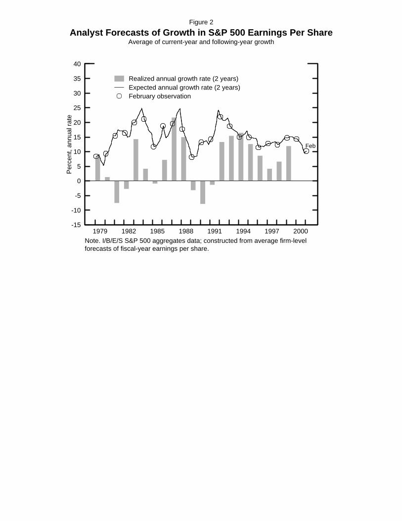
Figure 2

Analyst Forecasts of Growth in S&P 500 Earnings Per ShareAverage of current-year and following-year growth

-15

-10

-5

0

5

10

15

20

25

30

35

40

1979 1982 1985 1988 1991 1994 1997 2000

Feb

Note. I/B/E/S S&P 500 aggregates data; constructed from average firm-levelforecasts of fiscal-year earnings per share.

Per

cent

, ann

ual r

ate

Realized annual growth rate (2 years)Expected annual growth rate (2 years)February observation

13

14 Even ignoring the problem arising from negative earnings, the long-term growthforecast is a fairly ambiguous concept, and is interpreted in different ways by different analysts. Some treat it literally as the expected growth rate from the recent base, while others apply acyclically-adjusted concept, such as a peak-to-peak growth forecast. Moreover, there is no clearconsensus on the horizon analysts have in mind. Thus, rather than impose more structure, I letthe empirical results influence the interpretation.

15Prior to 1992, there are several quarters in which no survey value exists; sometimesvalues are missing for two of a year’s four quarters. In contrast, there are no missing values inthe Philadelphia Fed’s survey of 4-quarter inflation expectation series, which is highly correlatedwith the 10-year expectation series. I fit a 3-region spline regression of the 10-year expectationon the 4-quarter expectation to construct estimates of the 10-year expectation in those quarterswith missing values.

company’s weight is set equal to the maximum of the forecasts for the current and following

years’ earnings. In the rare circumstance where both are negative, the firm receives zero

weight.14

The resulting series is depicted by the solid line in Figure 3. The sample period is limited

further by this series, because firm-level estimates only became widely available in the I/B/E/S

data in 1983. As can be seen from the right-hand scale, historically, this series has moved within

a relatively narrow band; it also displays a high degree of autocorrelation. As one might expect,

the long-term growth forecast was relatively high in early 1983, when the economy had just

emerged from a deep recession. Similarly, growth expectations peak again in 1992, on the heels

of the 1990-91 recession. But the most striking feature of this series is the

unprecedented rise beginning in mid-1995.

Shown alongside the long-term growth forecast is the expected inflation rate over the next

10 years, as gauged by the quarterly Philadelphia Fed survey of professional forecasters (taken in

the second month of each quarter).15 The figure shows a negative relationship between expected

long-term inflation and expected long-term nominal earnings growth, which implies an even

stronger negative correlation between expected inflation and real, or inflation-adjusted expected

long-term growth. This foreshadows one of the main conclusions of this study: at least in part,

inflation is associated with low stock valuations at least because higher inflation with lower real

earnings forecasts.

Figure 3

Analyst Forecasts of Long-term Nominal Growth in S&P 500 EarningsVersus Expected Inflation

2

3

4

5

6

7

8

9

1980 1983 1986 1989 1992 1995 1998 2001 9

10

11

12

13

14

15

Note. Weighted average of expected nominal long-term earnings growth ratesfor S&P 500 constituents. For each company, expected growth is the I/B/E/Sconsensus (median analyst) forecast of the expected annual growth rate ofoperating earnings over the next three to five years.

Expected 10-year inflation rate(left scale)

Long-term growth forecast*(right scale)

Per

cent

, ann

ual i

nfla

tion

Per

cent

, ann

ual g

row

th

Feb

14

(8)

B. Methodology for hypothesis testing

To test model (5) and the value-relevance of analysts’ aggregated expectations, I estimate

the following regression using quarterly data:

where the time subscript is suppressed for notational simplicity. Consistent with the timing of

the expected inflation survey, other variables are measured in the middle month of each quarter.

The dependent variable is the ratio of the current S&P500 price to 12-month-lagging

earnings per share (equation (5) is multiplied through by !1). As just described, the independent

variables g1, g2, and gLT represent analyst forecasts of EPS growth for current year, the following

year, and the “long term”. For reasons explained below, the regression analysis is performed on

real, or inflation-adjusted, variables. Earnings forecasts are transformed into real growth

forecasts by deducting expected inflation, that is, by subtracting the expected four-quarter

inflation rate from g1 and g2 and the 10-year expected inflation rate from gLT. The variable

log(payout0) is the log of the lagged dividend payout rate; being a ratio of two nominals, no

transformation is required. Also appearing in the regression is a vector of variables (Z)--most

notably, expected 10-year inflation--that are hypothesized to be factors in long-run expected

equity returns. Finally, the random disturbance term, u, is assumed to be stationary and

uncorrelated with the explanatory variables. The benchmark specification assumes u to follow a

1st-order autoregressive process.

C. Predicted coefficients: earnings and dividend variables

Any textbook valuation model would imply positive betas on the earnings growth and

dividend payout variables. Under the assumption that key variables are not mismeasured or

omitted, equation (5) offers more specific predictions. In particular, the model implies that the

coefficients on g1 and g2 should equal 1.0 and D, respectively (where, again, D is slightly less than

one, such as 0.95). The coefficient on gLT should be positive and exceed 1. More precisely, if

this statistic represented expected growth over the next T years, the coefficient on gLT should

15

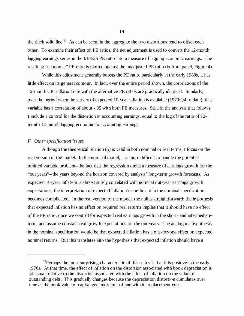
equal . For instance, if it represented a 5-year expectation as often advertised, the

predicted coefficient would be about 4.5. Even so, the potential redundancy from including g1

and g2 in the regression may reduce the coefficient on long-term growth (as well as on g1 and g2).

On the other hand, to the extent that expected growth beyond 5 years–the omitted variable–is

correlated with gLT, the coefficient on gLT may be inflated.

The model also puts restrictions on ", the coefficient on the log dividend payout rate. As

shown earlier, the assumed autoregressive behavior of the payout rate implies that " should fall

between 0 and 1. Moreover, the upper end of that range can be ruled out if shocks to the payout

rate are not extremely persistent, that is, if 1!8 is too close to 1. In a simple annual regression of

the log payout rate on its 12-month lag, I estimate a coefficient of about 0.75 on the lag. Thus,

the autoregressive parameter perceived by investors arguably ought to be reasonably close,

perhaps within a range like 0.6 to 0.9. With D=0.96, this translates into a point estimate for "

equal to 0.11, and plausible range of 0.06 to 0.27. Thus, the model suggests that, by itself, a

temporary change in the current dividend payout rate should have little effect on equity prices.

For instance, a 10 percent decline in the current dividend payout rate (holding earnings constant)

should only raise stock prices between 0.6 and 2.7 percent.

D. Proxies for expected returns

Assuming these variables adequately control for earnings and dividend growth

expectations, then, in a regression such as (6), any residual effect of expected inflation on the log

price-earnings ratio would reflect its effect on expected, or required, long-run returns. Of course,

such a test is based on the null hypothesis that expected stock returns are not time-varying, a null

that most of the profession would probably now view as a strawman. A more interesting

question is whether expected inflation is a significant factor for expected stock returns once we

control for other factors viewed as plausible conditioning variables for expected returns.

Researchers have documented a strong commonality between expected returns on stocks

and expected returns or yields on bonds [e.g., Keim and Stambaugh (1986), Campbell (1987),

Fama and French (1989)]. The most familiar characterization is the finding that the excess

returns on stocks versus short-term riskless bonds is positively related to ex ante term premia on

long-term bonds. The analogy to conditioning excess stock returns on the term premium would

16

16Another measurement issue arises from the distinction between “reported” and“operating” earnings. Firm-level studies of the relationship between earnings and stock pricesthat use reported earnings, such as “net income before extraordinary items” from Compustat,tend to find relatively small effects of changes in earnings on stock prices. Such studies areprobably hampered by the presence of large jumps in earnings associated with unusual (but not“extraordinary”) events, particularly restructuring charges and capital gains or losses on asset

be to condition stock returns on the long-term bond yield. Thus, in some regressions, I include

the expected real yield on 30-year Treasury bonds, defined as the 30-year Treasury bond yield

less the expected 10-year inflation rate.

Previous findings and most models predict a negative coefficient for the expected real

long-term bond yield: ceteris paribus, high real interest rates indicate a high required return, and

thus a low current stock price. Under the hypothesis that investors require a constant return

premium on stocks versus bonds--or an equity premium that is uncorrelated with expected real

bond returns--the model offers a sharper prediction. For instance, assuming a constant risk

premium and a flat term structure for expected one-period returns, then the coefficient on the

Treasury bond yield should equal !1/(1!D), the sum of the weights on expected future one-

period returns in equation (5), which equals !25 for D=.96.

As shown by Fama and French (1989), default risk spreads also appear to be an important

class of conditioning variables for long-horizon stock returns. They find that long-run stock

returns are positively related to an ex ante default risk spread, and argue that this variable serves

as a proxy for a long-term cyclical component in expected returns. Thus, I also include a default

risk spread as a conditioning variable for expected returns; in particular, I use the spread between

yields on Baa-rated and Aaa-rated industrial bonds, based upon Moody’s monthly bond yield

indexes. Like the long-term bond yield, this variable is expected to have a negative effect on the

price-earnings ratio.

E. Distortions to accounting earnings

A potentially important measurement problem that confronts any earnings-based

valuation model is that accounting earnings are a noisy measure of true economic earnings. Of

particular concern in this study are the discrepancies between accounting earnings and economic

earnings that are exacerbated by inflation.16 Indeed, inflation-induced distortions to earnings

17

sales. Such events often reflect information already in the public domain, and which areexpected to have little effect on earnings going forward. This type of measurement issue isavoided by using I/B/E/S data for actual historical (as well as expected) earnings.

17See von Furstenburg and Malkiel (1977), Shoven and Bulow (1976, 1977), and Scanlon(1981). Feldstein and Summers (1978) and Feldstein (1980) examine measurement distortionsassociated with inflation and how they interact with effective tax rates.

18For example, the stochastic process assumed for the log payout rate in (5) is lesscompelling in the presence of accounting distortions. In the presence of such distortions, theexpected dynamics of the expected (log) payout rate will depend not only on the expectedevolution of the true payout rate, which is arguably cyclical, but also on the expected dynamicsof any distortions to measured earnings.

caused by historical cost accounting was a topic of great interest and concern in the 1970s and

early 1980s, and a number of studies attempted to characterize and gauge these distortions.17

In principle, distortions in accounting earnings need not distort estimates of expected

return generated by our model. This is because the ultimate source of value in (5) is the

discounted stream of expected dividends; that is, this model is merely a rearrangement of the

terms in Campbell and Shiller (1988), in which expected return is calculated as a function of

dividend growth and the dividend price-ratio. As shown in the appendix, as long as earnings and

expected earnings are measured in a consistent fashion, any measurement problem embodied in

the earnings-price ratio and the earnings growth terms would be offset by distortions in the

dividend payout terms--the n’s--with equal and opposite effect.

Nonetheless, in practice, the presence of accounting distortions is likely to bear on the

validity of any particular set of assumptions on unobservables, such as the assumed dynamics of

the expected payout rate or assumptions regarding the expected growth of (accounting) earnings

beyond analysts’ forecast horizons.18 Thus, I construct a control variable that measures the

wedge between lagged accounting and economic earnings.

As emphasized by Modigliani and Cohn (1979), and more recently by Ritter and Warr

(2000), high inflation amplifies two prominent distortions in accounting profits: (i) the

understatement of economic depreciation expense by accounting “book-value” depreciation, and

(ii) the overstatement of economic debt-service expense by reported interest expense. The size of

these distortions in S&P500 earnings can be gauged using data from the National Income and

Product Accounts (NIPAs), under the assumption that the distortions are spread proportionally

18

19The current cost adjustment is one of two pieces that constitute the capital consumptionadjustment in the NIPAs, and is only available annually; the annual series is converted to amonthly series using a linear smoothing algorithm. The other piece of the NIPA capitalconsumption adjustment, unneeded for our purposes, converts depreciation from the tax-basedmeasure in NIPA source data to economic depreciation (at historical cost).

20The inflation rate is the four-quarter percent change in the GDP deflator. The aggregatebook value of debt is taken to be the outstanding amount of credit market instruments, net ofinterest-earnings assets on the balance sheet of nonfinancial corporations in the U.S., asestimated from table L.102 in the Flow of Funds Accounts published by the Federal Reserve. This omits any such distortion associated with financial corporations’ profits, but the distortionarising from that sector probably contributes little to the total since the financial sector accountsfor only about 20 percent of total profits; moreover, the net debt position of financial institutionstends to be small because of their offsetting investments in debt.

throughout the aggregate U.S. corporate sector.

The extent to which earnings are overstated as a result of historical cost-based

depreciation methods can be estimated using the NIPA current-cost adjustment, the component

of the capital consumption adjustment that converts aggregate U.S. corporate depreciation from a

book-value basis to a replacement-cost basis. This adjustment, expressed as a fraction of total

after-tax NIPA profits, is shown by the light solid line the upper panel of figure 4. It grows more

negative during the period of rising inflation and then only gradually reverts back toward zero

after inflation falls off in the early 1980's.19

The interest expense reported in financial statements tends to overstate true economic

debt-service expense because the portion of interest expense that compensates creditors for

inflation is not an economic expense; rather, as explained quite thoroughly by Ritter and Warr

(2000), it represents compensation for the gain a debtor realizes when inflation depreciates the

value of its nominal liabilities. I construct an adjustment for depreciation of real net liabilities in

the U.S. corporate sector by multiplying the book value of debt outstanding on the balance sheet

of nonfinancial U.S. corporations by the contemporaneous inflation rate.20 The resulting

adjustment, again expressed as a fraction of aggregate after-tax profits, is shown by the dotted

dashed line in the upper panel of figure 4.

Finally, the net adjustment that results from summing these two adjustments is plotted by

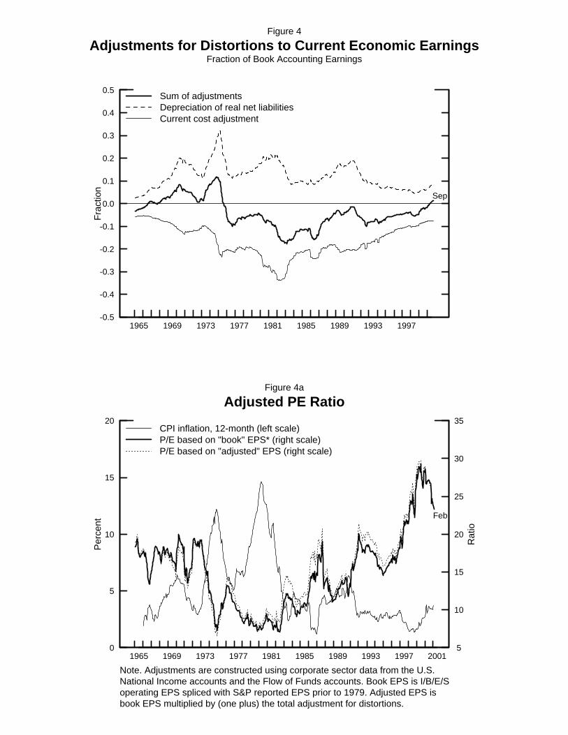
Figure 4

Adjustments for Distortions to Current Economic EarningsFraction of Book Accounting Earnings

-0.5

-0.4

-0.3

-0.2

-0.1

0.0

0.1

0.2

0.3

0.4

0.5

1965 1969 1973 1977 1981 1985 1989 1993 1997

Fra

ctio

n

Sep

Sum of adjustmentsDepreciation of real net liabilitiesCurrent cost adjustment

0

5

10

15

20

1965 1969 1973 1977 1981 1985 1989 1993 1997 2001 5

10

15

20

25

30

35

Note. Adjustments are constructed using corporate sector data from the U.S.National Income accounts and the Flow of Funds accounts. Book EPS is I/B/E/Soperating EPS spliced with S&P reported EPS prior to 1979. Adjusted EPS isbook EPS multiplied by (one plus) the total adjustment for distortions.

Figure 4a

Adjusted PE Ratio

Per

cent

Rat

io

Feb

CPI inflation, 12-month (left scale)P/E based on "book" EPS* (right scale)P/E based on "adjusted" EPS (right scale)

19

21Perhaps the most surprising characteristic of this series is that it is positive in the early1970s. At that time, the effect of inflation on the distortion associated with book depreciation isstill small relative to the distortion associated with the effect of inflation on the value ofoutstanding debt. This gradually changes because the depreciation distortion cumulates overtime as the book value of capital gets more out of line with its replacement cost.

the thick solid line.21 As can be seen, in the aggregate the two distortions tend to offset each

other. To examine their effect on PE ratios, the net adjustment is used to convert the 12-month

lagging earnings series in the I/B/E/S PE ratio into a measure of lagging economic earnings. The

resulting “economic” PE ratio is plotted against the unadjusted PE ratio (bottom panel, Figure 4).

While this adjustment generally boosts the PE ratio, particularly in the early 1980s, it has

little effect on its general contour. In fact, over the entire period shown, the correlations of the

12-month CPI inflation rate with the alternative PE ratios are practically identical. Similarly,

over the period when the survey of expected 10-year inflation is available (1979:Q4 to date), that

variable has a correlation of about -.85 with both PE measures. Still, in the analysis that follows,

I include a control for the distortion in accounting earnings, equal to the log of the ratio of 12-

month 12-month lagging economic to accounting earnings.

F. Other specification issues

Although the theoretical relation (5) is valid in both nominal or real terms, I focus on the

real version of the model. In the nominal model, it is more difficult to handle the potential

omitted variable problem--the fact that the regression omits a measure of earnings growth for the

“out years”--the years beyond the horizon covered by analysts’ long-term growth forecasts. As

expected 10-year inflation is almost surely correlated with nominal out-year earnings growth

expectations, the interpretation of expected inflation’s coefficient in the nominal specification

becomes complicated. In the real version of the model, the null is straightforward: the hypothesis

that expected inflation has no effect on required real returns implies that it should have no effect

of the PE ratio, once we control for expected real earnings growth in the short- and intermediate-

term, and assume constant real growth expectations for the out years. The analogous hypothesis

in the nominal specification would be that expected inflation has a one-for-one effect on expected

nominal returns. But this translates into the hypothesis that expected inflation should have a

20

22There is also a technical difficulty with the nominal model. Since fluctuations in out-year growth expectations is one source of the disturbance term, assuming the disturbance term isstationary requires the same of those out-year-growth expectations. But long-term nominalgrowth expectations are less likely to be stationary than real growth expectations, given theevidence of potential nonstationarity in the inflation rate (e.g., Campbell and Shiller, 1989).

large negative effect on the price-earnings ratio via the expected return channel, tempered by the

unobserved and indeterminate effect of expected inflation on expected nominal earnings growth

in the out-years.22

V. Empirical Results

A. Simple Correlations

Simple correlations are shown in Table 1. In order to illustrate the most basic relations,,

Pearson correlations are calculated using nominal (unadjusted) earnings growth variables and

bond yields. As shown in the first column, the PE ratio is negatively correlated with the

dividend payout rate. It is positively correlated with forecasts of long-term earnings growth

forecasts, while its correlations with forecasts of near-term earnings growth are less apparent.

The PE ratio’s correlation with the Treasury bond yield mimics its strong negative correlation

with expected inflation. As one might expect, the PE ratio is negatively related to the bond

default premium and positively correlated with earnings quality.

B. Main regression results

The four columns of table 2 show results from regressions of the log price-earnings ratio

on expected inflation and various combinations of the model variables; together they illustrate

how much inflation’s explanatory power is diminished by controlling for fundamentals. All

specifications include the control for earnings quality, equal to the log of the ratio of economic to

accounting earning. Finally, these specifications include an AR(1) disturbance term, estimated

via the Yule-Walker method. The regression R-squared measures the R-squared on the

transformed variables, that is, the explanatory power of all variables except the AR(1) term.

The first column reports the regression with expected 10-year inflation as the only

explanatory variable, which serve as a benchmark for gauging subsequent results. The

21

23Indeed, the payout rate does get a negative coefficient when I regress the PE ratio onthe payout rate by itself, or with just the year 1 and year 2 growth forecasts.

coefficient on expected inflation, -20.08, is sizable, implying that a 1 percentage point increase in

the expected 10-year inflation rate is associated with a 20 percent decline in the price-earnings

ratio, or a 20 percent decline in stock prices given lagged earnings. The AR(1) coefficient

estimate is 0.79, large though significantly less than unity.

The second regression adds the variables measuring earnings and dividend growth

expectations. Adding these variables boosts the R-squared to 0.88 and reduces the AR(1) term.

Overall, the coefficient estimates are quite supportive of the model and the joint hypothesis that

analyst earnings forecasts are value-relevant. The coefficients on g1 and g2 are both positive and

significant; at 0.76 and 0.98, neither is significantly different from its theoretical value. The

coefficient on long-term growth is positive, significant, and quite large; at 9.4, it is about twice

the magnitude predicted by theory if it represented a five-year forecast.

The coefficient on the payout rate variable is positive as predicted by the model.

Although it is more than double our point prediction of 0.13 (implied by an autoregression of the

log payout ratio on its 12-month lag), it is consistent with plausible speeds of mean reversion in

the payout ratio. It is interesting to note that the coefficient on the payout rate could have been

negative if the payout rate in this regression primarily served as a proxy for expected returns, as it

apparently does in Lamont’s (1998) regressions, where a high payout rate predicts high future

returns.23

Regarding the main hypothesis of interest, adding the proxies for real growth expectations

to the regression only dampens the coefficient estimate on expected inflation to !15, or by 25

percent compared with column (1). Thus, regression (2) results clearly reject the hypothesis that

long-run required real stock returns are constant in favor of the alternative that they are positively

related to expected inflation.

Arguably, the more interesting question is whether inflation has independent predictive

power for long-run expected returns once we admit other factors that are thought to predict long-

run returns. A test of this hypothesis is provided by the regression in column (3), which adds two

proxies for expected long-run returns--the real 30-year Treasury bond yield and the default

22

24At !6.7, this coefficient is modest in magnitude. The hypothesis that expected long-runstock returns move one-for-one with the real bond yield predicts a value around !25.

premium on Baa-rated bonds. As shown, the estimated coefficient on the expected real bond

yield is negative and statistically significant.24 The coefficient on the default premium is negative

but very small and statistically insignificant. Coefficients on the earnings growth variables are

little changed from (2). The coefficient on long-term earnings growth expectations is again quite

large; it suggests that a 1 percentage point increase in expected growth increases stock prices 10.6

percent. Finally, with the addition of these proxies for expected return, the coefficient on

expected inflation is trimmed to !5.2 and is no longer significant. Thus, once we control for both

expected earnings and bond yields, expected inflation no longer helps to explain equity prices.

Based upon regressions (2) and (3), one might conclude that the correlation between

equity valuations (PE ratios) and expected inflation arises largely from the positive association

between expected inflation and expected returns. However, this notion is countered by

specification (4), where bond yields are included and earnings growth variables are excluded.

Here, the coefficient estimate on expected inflation is !17, similar to regression (2). Hence, we

are led to the conclusion that both influences--an earnings growth effect and a required return

effect--are behind the correlation between inflation and stock valuations. Only when we control

for both factors can we explain away the apparent effect of inflation on equity prices.

C. Robustness

I consider some alternative specifications to address a couple robustness issues: How

sensitive are the results to the assumed dynamics? And, to what extent are they driven by the

extraordinary observations from the last few years? Specification (5) begins with (3) but

excludes the AR(1) term. Specification (6) instead employs a partial-adjustment (error-

correction) specification; that is, it includes a lagged dependent variable in place of the AR(1)

term. To facilitate comparisons, coefficients shown for (6) are the implied long-run coefficients,

b/(1-8), along with the coefficient on the lagged dependent variable, 8. In both (5) and (6), the

Newey-West method is used to compute heteroskedasticity and autocorrelation-consistent

standard errors.

23

As shown in table 3, specifications (5) and (6) yield conclusions that are quite consistent

with the base case. The coefficient on expected inflation remains relatively small, though in (5)

it is statistically significant. Also, in both cases, the estimated effect of long-term growth

expectations remains quite large. Perhaps the only notable difference is the somewhat smaller

pair of coefficients on the shorter-term growth forecasts in (6).

Specification (7) allows us to gauge how sensitive the results are to excluding the

extraordinary period of high equity valuations, when long-term growth forecasts similarly were at

record highs. In particular, I estimate the base case model (3) on a subsample that ends in 1996.

Indeed, in this subsample the coefficient estimate on expected inflation is more negative (-10.96

versus -5.2) and statistically significant. At the same time, the coefficient on the long-term

growth forecast shrinks to 4.0, significant only at the 10 percent level. Thus, excluding the recent

four-year period does temper the strength of the earlier conclusions.

Nonetheless, given the relatively short sample, eliminating some of the data reduces our

ability to identify the separate effects of highly correlated variables. For instance, if the earnings

growth forecast for year 2 is excluded from this shorter sample regression, the coefficient on

long-term growth is boosted to -7.7, and is significant at the 1 percent level, while the coefficient

on expected inflation is diminished. Alternatively, under the hypothesis that expected inflation’s

effect on equity valuation is spurious, its inclusion in the regression could bias down the

coefficient on long-term growth, given their strong negative correlation. Indeed, as shown in

column (8), if expected inflation is excluded from the regression, then the coefficient on long-

term growth rises to 9.6 and is once again statistically significant.

D. Interpreting the effect of long-term growth expectations

Given the importance of analysts’ long-term growth forecasts in the results, our

interpretation depends critically on the maintained hypothesis, adopted from the accounting

literature, that such forecasts are exogenous with respect to stock prices. Previous findings

suggest that most types of forecasts by equity analysts violate rational expectations of future

earnings, though the properties of long-term growth forecasts have received less attention than

shorter-term forecasts. Still, research indicates that analysts’ long-term forecasts are not only

upward biased but also too extreme, or more upward biased for firms expected to grow fast [e.g.,

24

25What is more, to the extent that forecasts are updated after a slight lag, even if forecasts weretruly exogenous with respect to prices, under rational expectations market prices could still cause analystforecasts in a Granger sense.

(9)

Dechow and Sloan (1997), Rajan and Servaes (1997)]. There is also mixed support for the view

that analysts over-extrapolate from recent observations [De Bondt (1992), La Porta (1996)].

Such qualities do not necessarily invalidate the utility of these forecasts for explaining

stock valuations, and they may well represent analysts’ best efforts, even if subject to some

institutional constraints. The more problematic issue is the possibility that analysts adjust their

growth forecasts in response to stock prices. Such behavior could reflect a cynical attempt to

justify current stock prices or the sincere efforts of Bayesian analysts trying to incorporate others’

information reflected in stock prices; either way, if pervasive, this would cause these regressions

to be plagued by simultaneity bias.

Given our relatively short time series and the degree of autocorrelation in long-term

growth forecasts, simple time series tests of exogeneity are not likely to be very convincing.25

Still, some indication of earnings forecast exogeneity might be had by examining whether the

estimated errors from our valuation model have substantially greater ability to predict stock price

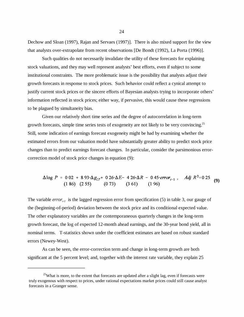
changes than to predict earnings forecast changes. In particular, consider the parsimonious error-

correction model of stock price changes in equation (9):

The variable errort-1 is the lagged regression error from specification (5) in table 3, our gauge of

the (beginning-of-period) deviation between the stock price and its conditional expected value.

The other explanatory variables are the contemporaneous quarterly changes in the long-term

growth forecast, the log of expected 12-month ahead earnings, and the 30-year bond yield, all in

nominal terms. T-statistics shown under the coefficient estimates are based on robust standard

errors (Newey-West).

As can be seen, the error-correction term and change in long-term growth are both

significant at the 5 percent level; and, together with the interest rate variable, they explain 25

25

(10)

(11)

percent of the variation in price changes. To gauge the marginal contribution of the long-term

growth forecast, this equation was re-estimated with two changes: )gLT was excluded and the

lagged error was extracted from a P/E ratio regression that excluded long-term growth. The

adjusted R-squared drops to 0.15 in this version, a substantial fall-off from the result in (9).

To gauge the reverse causation, that is, the influence of stock prices on growth forecasts,

we estimate a similar regression but with long-term growth (scaled by 100) as the dependent

variable:

In this case, the adjusted R-squared is only 0.02, suggesting that little variation in analysts’ long-

term growth forecast is explained by stock price changes or the lagged valuation error. Price has

a small positive effect, significant only at the 0.13 level. More importantly, the error-correction

term has no effect on growth forecasts. Taken together, (9) and (10) thus provide some support

for adopting the customary working assumption that analysts’ long-term growth forecasts are

exogenous with respect to equity prices.

VI. A direct test of inflation’s effect on the equity premium

The evidence on the validity of the model and its application to the survey data provide

reasonable support for using the model to construct an explicit ex ante measure of expected long-

run stock returns. I construct such a measure of expected real stock returns as follows:

where D= 0.96 and "=0.15. As in the regression analysis, the g’s are converted into real growth

forecasts by subtracting inflation expectations. To be roughly consistent with the size of the

coefficient estimates on gLT in the PE ratio regressions (tables 2,3), the long-term growth forecast

26

26This assumed horizon would be consistent with a coefficient of 8.34 in the PEregressions. Admittedly, this approach to choosing a horizon is somewhat circular; but thissection is not thought of as generating inferences on the equity premium that are independent ofearlier results. In any case, changing the assumed horizon by a few years has no material affecton the conclusions to follow.

27 Of course, given the decline in expected long-run inflation, expected nominal returnson stocks have declined much more than expected real returns.

is treated as a forecast for a 10-year period, from year 3 to year 12.26 The flip side of this

assumption is that expected real earnings growth beyond year 12 is assumed to be constant, or at

least stationary.

The constant C is unobservable and influenced by three factors: (i) expected real growth

in the out years, (ii) the bias investors impute to analyst earnings forecasts, and (iii) the expected

long-run dividend payout rate. Thus, expression (11) only allows us to gauge the relative level of

expected returns over time. For purpose of illustration, the estimates are arbitrarily anchored by

assuming the expected real return on equity equaled 7 percent in February 1989.

The resulting estimates of expected long-run real equity returns are plotted in Figure 5;

and shown alongside is the expected real yield on the 30-year Treasury bond. (Note that the scale

for the bond yield–on the left side–is the same as that for the expected equity returns, only shifted

up two points to facilitate visual comparison.) The estimates imply that expected real equity

returns in early 2001 were about 1 percentage points lower than in 1989, and nearly 3 percentage

points lower than in 1984.27 These estimates thus suggest that the downward post-war trend of

required equity returns identified by Blanchard (1993) has yet to abate. Perhaps the more striking

aspect of figure 5 is the apparent positive correlation between the required return on equity and

the expected real yield on the 30-year bond, at least until 1998. This relationship contrasts with

Blanchard’s other main conclusion--that the real return required on Treasury bonds was

negatively related to the required return on equity. This disparity might owe to a shift in behavior

around the early 1980s; but methodological differences--my use of survey-based expectations--is

also likely to be an important factor.

The relationship between the expected return on equity, bond yields, and inflation

expectations are summarized by a few simple regressions in Table 4. The first two columns

Figure 5

Long-Run Expected Return: S&P 500 vs. 30-year Bond

2

3

4

5

6

7

8

1983 1985 1987 1989 1991 1993 1995 1997 1999 2001 4

5

6

7

8

9

10

Real bond yield

Real expected equity return

Yie

ld (

Per

cent

)

Ret

urn

(Per

cent

)

Note. The level of the expected equity return series is pinned down with theassumption that the expected long-run real return equaled 7% in 1989:Q1.

Feb

27

28Summers (1983) argues that bond yields should increase by more than expectedinflation. However, his empirical analysis of bond yields and inflation over a variety of periods,the most recent being 1954-1979, suggested that bond yields tend to change by less than changesin expected inflation. My analysis differs in that it uses survey data to measure expectedinflation; moreover, the time period analyzed above begins about where Summers’ sampleperiod ends.

29This suggests that the inflation-hedging benefits of inflation-indexed bonds may beeven stronger than intimated by Campbell and Viceira (2001).

show results of regressions where the dependent variable is the expected long-run real return on

the S&P 500. The first regression measures the univariate relationship between expected real

stock returns and expected long-term inflation. The coefficient estimate of 0.66 suggests that a 1

percentage point rise in expected long-term inflation raises the expected long-run real return on

equity by two-thirds of a percentage point. The second column considers a multivariate model of

expected equity returns, adding the real 30-year Treasury bond yield, the default premium (AAA-

BAA yield spread), and the term premium on Treasuries (the spread between the 30-year and 3-

month Treasury yields) as explanatory variables. Whereas the bond yield helps explain expected

equity returns, its coefficient is far from one, and the latter two regressors are not significant,.

In the third regression, the dependent variable is the expected long-run return premium on

equity, defined as the expected real return on equity less the expected real yield on the Treasury

bond. The results strongly suggest that the expected return premium is independent of the default

and term premia. Perhaps most interesting, though, is the finding that the return premium is

unrelated to expected inflation, consistent with the results of the P/E ratio regressions. This

finding suggests that, at least over the last two decades, expected inflation’s effect on the return

required on long-term bonds is similar to the effect on required equity returns.28 This conjecture

is verified by the last column of Table 4, which shows the result from regressing the real long-

term bond yield on expected inflation. The coefficient of 0.75 suggests that a 1 point rise in

expected long-run inflation is accompanied by a 3/4 point rise in long-term real yields.29

VII. Summary, Interpretation, and Conclusion

Over the last several decades, equity valuations, as measured by price-earnings ratios,

have exhibited a strong negative relation with both actual and expected inflation, a regularity that

28

cannot be explained by inflation-induced distortions to accounting earnings. According to the

present discounted value model, this implies that high inflation presages either high long-run real

equity returns or low long-run real earnings growth (holding constant the path of dividend payout

rates). My empirical analysis provides evidence to suggest that both factors are at play. Market

expectations of real earnings growth, particularly longer-term growth, are negatively related to

expected inflation. But even after controlling for these earnings forecasts, equity valuations (PE

ratios) are negatively affected by expected inflation, suggesting that inflation also increases the

required long-run return on stocks. However, most, if not all, of the inflation-related component

in expected stock returns is also in real bond yields. Thus, during the period analyzed in this

study, the expected equity risk premium over long-term Treasury bonds appears to be

uncorrelated with expected inflation.

One plausible explanation for the positive effect of expected inflation on required real

stock and bond returns is an inflation-induced distortion to real effective tax rates on personal

investment income [e.g., Feldstein (1980b)]. Because investors pay taxes on their nominal

capital income from both stocks and bonds–both the real return as well as the component that

compensates investors for depreciation of principal–inflation reduces after-tax real returns; thus,

investors are likely to respond by demanding higher real pretax returns.

One question raised but not answered by our findings is why higher long-run inflation

expectations are associated with forecasts of lower growth in real--not to mention nominal--

earnings. One possibility, of course, is that increases in inflation, even modest increases–result in

resource mis-allocation, lower productivity, and slower growth in economic activity. Another

possibility that must be given some consideration, even if distasteful to economists, is that

investor perceptions may be distorted by inflation.

In their controversial analysis of inflation and equity valuation, Modigliani and Cohn

(1979) documented a similar negative relationship between the PE ratio and inflation. While

they acknowledged the logical possibility that such a relation could reflect an inflation-related

risk premium on stocks relative to bonds, they argued that the magnitude of the effect was

difficult to rationalize. The more plausible explanation, they argued, is that investors are plagued

by a form of money illusion; in particular, “investors capitalize equity earnings at a rate that

parallels the nominal interest rate on bonds, rather than the economically correct real rate--the

29

nominal rate less the inflation premium.”

But the Modigliani-Cohn analysis assumes that long-run real earnings growth

expectations are essentially constant, and imposes some very specific assumptions on the

structure of near-term earnings forecasts as well. In particular, their valuation model assumes

that investors capitalize a measure of recent profits, adjusted for the current state of the business

cycle (and accounting distortions), a measure they call “long-term profit”. Thus, their study

abstracts from a major piece of our explanation--that real earnings growth forecasts are

negatively related to inflation.

Nonetheless, in an important sense, the Modigliani-Cohn hypothesis, that equity prices

are distorted by money illusion, could well have been close to the mark. Rather than

inappropriately discounting real earnings with a nominal interest rate, it could be that investors

use a nominal interest rate to discount expected nominal earnings, where those nominal earnings

forecasts are themselves contaminated by money illusion; that is, they might fail to “rationally”

incorporate inflation expectations.

Analysts’ forecasts of individual firms’ earnings--figures that are always discussed in

nominal terms--most commonly appear to be anchored in nominal sales growth projections that

are extrapolated from recent historical trends. If analysts fail to make adjustments to those trends

in response to shifts in the expected long-term inflation rate, then increases in inflation will have

the effect of reducing implicit forecasts of real earnings growth. Indeed, Ritter and Warr (1999)

show that some recent and relatively sophisticated applications of accounting earnings-based

valuation models (e.g., Lee, Myers and Swaminathan (1998)) make no allowance for inflation in

their assumptions on long-horizon nominal earnings trajectories. Moreover, they show that the

ability of such models’ to explain valuations deteriorates when an adjustment for inflation is

incorporated into long-horizon residual profit forecasts.

Similarly, few practitioners seem to perceive much benefit from analyzing accounting

data and earnings forecasts in real, or inflation-adjusted, terms. One explanation for this might be

that the results of simple empirical analyses, such as in Keon (1999), contradict the classical

economic presumption that higher inflation translates into higher nominal profit, at least over the

short and medium run. In any case, an examination of the determinants of earnings forecasts and

their relation to expected inflation should constitute an informative direction for future research.

30

(12)

(13)

Appendix: Earnings Measurement Error

To examine the issue of measurement error, let Qt / EPSt/EPSta , where EPSt

a denotes

book accounting earnings and EPSt denotes economic earnings. The variable Qt is meant to

represent the “quality” of reported earnings. In an inflationary environment, book accounting

earnings are generally thought to overstate true earnings; that is, Q < 1. Define the following :

To show that equation (1) also holds in terms of accounting earnings EPSa; let q / log(Q), and

substitute log(EPSa) + q for log(EPS) in (1). Doing so yields:

But it is straightforward to confirm that the right-hand side terms involving q’s sum up to qt, the

left-hand-side term; that is,

Thus, in principle, using accounting earnings does not bias the implied estimate of long-

horizon returns.

31

References

Bakshi, G. S., and Z. Chen, “Inflation, asset prices, and the term structure if interest rates inmonetary economies,” Review of Financial Studies, 9 (Spring 1996), 241-276.

Barnes, Michelle, John H. Boyd, and Bruce D. Smith, “Inflation and Asset Returns,” EuropeanEconomic Review 43 (1999), 737-754.

Bernard, Victor L., “Unanticipated inflation and the value of the firm,” Journal of FinancialEconomics 15 (1986), 285-321.

Blanchard, Olivier J., “Movements in the equity premium,” Brookings Papers on EconomicActivity (1993, no. 2), 75-138.

Bodie, Z., “Common stocks as a hedge against inflation,” Journal of Finance, 31 (1976), 459-470.

Boudoukh, Jacob, M. Richardson, “Stock returns and inflation: A long horizon perspective,”American Economic Review, 83 (December 1993), 1346-1355.

Boudoukh, Jacob, Matthew Richardson and Robert F. Whitelaw, “Industry returns and the fishereffect,” Journal of Finance 49 (December 1994), 1595-1614.

Brown, Lawrence D., “Earnings Forecasting Research: Implications for Capital MarketsResearch,” International Journal of Forecasting 9 (1993), 337.

Campbell, J., 1998, “Asset prices, consumption, and the business cycle,” in John G. Taylor andMichael Woodford (eds), Handbook of macroeconomics, Vol. 1 (Amsterdam: North-Holland,1999), 1231-1303.

Campbell, John Y. and John Ammer, “What moves the stock and bond markets? A variancedecomposition for long-term asset returns,” Journal of Finance 48 (March 1993), 3-37.

Campbell, J.Y., A.W. Lo and A.C. MacKinlay, The Econometrics of Financial Markets, 1997(Princeton: Princeton University Press), 302-304.

Campbell, John Y. and R. Shiller,“Stock prices, earnings, and expected dividends,” Journal ofFinance 43 (July 1988), 661-671.

Campbell, John Y. and R. Shiller,“The dividend-price ratio and expectations of future dividendsand discount factors,” Review of Financial Studies, 1 (1989), 195-228.

Campbell, John Y. and Luis M. Viceira, “Who should buy long-term bonds?” AmericanEconomic Review 91 (March 2001), 99-127.

32

Chen, Nai-Fu,“Financial Investment Opportunities and the Macroeconomy,” Journal of Finance46 (1991), 529-554.

Claus, James and Jacob Thomas, “The Equity Risk Premium is much lower than you think it is:empirical estimates from a new approach,” mimeo, Columbia Business School (1998).

De Bondt, W. F.M., Earnings Forecasts and Share Price Reversals, Charlottesville, Virginia: TheResearch Foundation of The Institute of Chartered Financial Analysis, 1992.

Dechow, P.M. and R.G. Sloan, “Returns to contrarian investment strategies: Tests of naiveexpectations hypotheses,” Journal of Financial Economics 43 (1997), 4-27.

Fama, E., “Stock Returns, real activity, inflation, and money,” American Economic Review 71(1981), 545-565.

Fama, E., and K. French, “Business conditions and expected returns on stocks and bonds ,”Journal of Financial Economics 25 (1989), 23-49.

Fama, E. F. and G. W. Schwert, “Asset Returns and Inflation,” Journal of Financial Economics, 5(1977), 115-146.

Feldstein, M., “Inflation, tax rules and the stock market,” Journal of Monetary Economics 6(1980a), 309-331.

Feldstein, M., “Inflation and the stock market,” American Economic Review 70 (1980b), 839-847.

Feldstein, M. and L. Summers,“Effects of inflation oon the taxation of capital income in thecorporate sector,” National Tax Journal 32 (1979), 445-470.

Fisher, Irving,“The theory of interest,” (New York: McMillan, 1930).

Frankel, Richard and Charles M.C. Lee, “Accounting valuation, market expectation, and cross-sectional stock returns,” Journal of Accounting and Economics, 25 (1998), 283-319.

French, K., R. Ruback, and G.W. Schwert,“Effects of nominal contracting on stock returns,”Journal of Political Economy 91 (1983), 70-96.

Froot, Kenneth A.,“New Hope for the Expectations Hypothesis of the Term Structure of InterestRates,” Journal of Finance 44 (1989), 283-306.

von Furstenberg, G., and Burton Malkiel, “Financial Analysis in an Inflationary Environment,”Journal of Finance 32 (1977), 575-588.

Geske, Robert, and Richard Roll,“The fiscal and monetary linkage between stock returns andinflation,” Journal of Finance 38 (1983), 1-33.

33

Hansen, L. and R. Jagannathan, “Restrictions on Intertemporal Marginal Rates of SubstitutionImplied by Asset Returns,” Journal of Political Economy, 99 (1991), 225-262.

Hess, Patrick J. and Bong-Soo Lee, “Stock Returns and Inflation with Supply and DemandDisturbances,” The Review of Financial Studies, 12 (1999, no. 5) pp. 1203-18.

Jensen, G., J. Mercer, and R. Johnson, “Business Conditions, monetary policy, and expectedsecurity returns,” Journal of Financial Economics 40 (1996), 213-237.

Kaul, G.,“Stock returns and inflation: The role of the monetary sector,” Journal of FinancialEconomics 18 (1987), 253-276.

Keim, Donald B. and Robert F. Stambaugh, “Predicting returns in the stock and bond markets,”Journal of Financial Economics, 17 (1986), 357-390.

Keon, Edward, “Long-term Equity Returns,” Prudential Securities Quantitative Research,November 11, 1999.

Lamont, Owen, “Earnings and Expected Returns,” The Journal of Finance 53 (October 1998),1563-1587.

La Porta, R., “Expectations and the cross-section of returns,” Journal of Finance 51 (December1996), 1715-1742.

Lee, Charles M.C., James Myers, and Bhaskaran Swaminathan, “What is the intrinsic value of theDow?” Journal of Finance, 54 (1999), 1693-1741.

Lintner, J., “Inflation and security return,”Journal of Finance, 30 (1975), 259-80.

Liu, Jing and Jacob Thomas, “Stock Returns and Accounting Earnings,” working paper,Columbia Business School (1999).

Marshall, D., ”Inflation and asset return in a monetary economy,” Journal of Finance, 47 (1992),1315-1342.

Modigliani, Franco, and R.A. Cohn, “Inflation and the stock market,” Financial Analyst Journal35 (1979), 24-44.

Nelson, William R., “The Aggregate Change in Shares and the Level of Stock Prices,” Financeand Economic Discussion Series no. 1999-08, Federal Reserve Board (1999).

Patelis, A.D., “Stock return predictability and the role of monetary policy,” Journal of Finance 52(1997), 1951-1972.

Pearce, D., and V. Roley, “Firm characteristics, unanticipated inflation, and stock returns,”

34

Journal of Finance 43 (1998), 965-981.

Rajan, R. and H. Servaes, “Analyst following of initial public offererings,” Journal of Finance, 51(June 1997), 507-529.

Ritter, Jay R. and Richard S. Warr, “The Decline in Inflation and the Bull Market of 1982 to1999, forthcoming, Journal of Financial and Quantitative Analysis (April 2001).

Rouwenhorst, K. Geert, “Asset Pricing Implications of Equilibrium Business Cycles,” in Frontiersof Business Cycle Research, Thomas F. Cooley, ed, (Princeton, New Jersey: Princeton UniversityPress, 1995), pp. 294-330.

Scanlon, Martha S., “Postwar trends in corporate rates of return,” in Public Policy and CapitalFormation: A study by the Federal Reserve System (Washington D.C., Board of Governors of theFederal Reserve, 1981).

Shiller, R., and A. Beltratti, “Stock prices and bond yields,” Journal of Monetary Economics 30(1992), 25-46.

Shoven, J., and J. Bulow,“Inflation accounting and nonfinancial corporate accounting: financialassets and liabilities,” Brookings Papers on Economic Activity (1976, no 3).

Stulz, R., “Asset pricing and expected inflation,” Journal of Finance 41 (1986), 209-223.

Summers, L. “Inflation and the valuation of corporate equities,” NBER working paper (1981).

Summers, L., “The nonadjustment of nominal interest rates: A study of the Fisher effect” in J.Tobin, ed., Macroeconomics, Prices, and Quantities (Washington, D.C.: Brookings Institution,1983) 201-224.

Thorbecke, W.,“On stock market returns and monetary policy,” Journal of Finance 52 (1997),635-654.

Table 1

Pearson Correlations of Quarterly Values

log P/E0 logpayout

growth(1) growth(2) long termgrowth

10-yr.inflation

4-qtr.inflation

30-yrbondyield

defaultpremium

log payout -0.59**

growth(1) -0.27* 0.66**

growth(2) 0.06 0.48** 0.51**

long termgrowth

0.77** -0.79** -0.35** -0.09

10-yr inflation

-0.89** 0.73** 0.53** 0.25* -0.68**

4-qtr inflation

-0.88** 0.59** 0.37** 0.06 -0.68** 0.92**

30-yr bondyield

-0.87** 0.54** 0.45** 0.14 -0.51** 0.93** 0.87**

defaultpremium

-0.65** 0.52** 0.44** 0.14 -0.38** 0.78** 0.67** 0.75**

earningsquality

0.61** -0.62** -0.62** -0.34** 0.52** -0.69** -0.47** -0.65** -0.65**

Correlations marked by * and ** are significant at the 5% and 1% level, respectively.

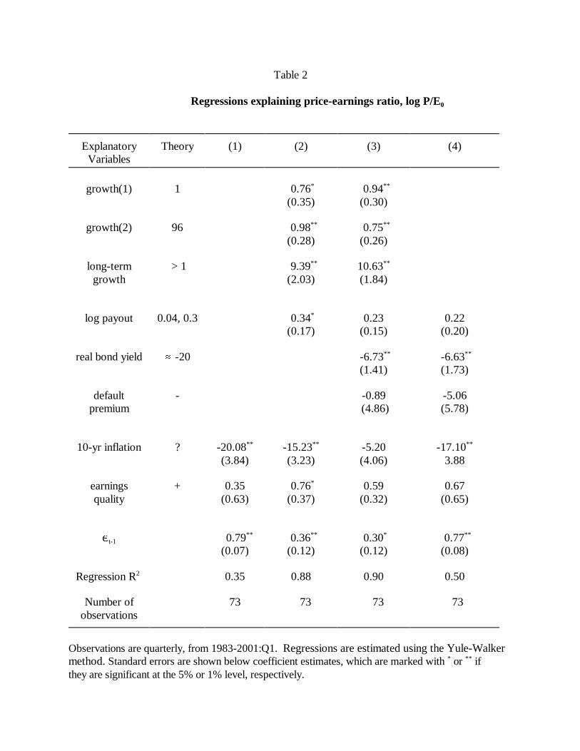
Table 2

Regressions explaining price-earnings ratio, log P/E0

ExplanatoryVariables

Theory (1) (2) (3) (4)

growth(1) 1 0.76*

(0.35) 0.94**

(0.30)

growth(2) 96 0.98**

(0.28) 0.75**

(0.26)

long-termgrowth

> 1 9.39**

(2.03)10.63**

(1.84)

log payout 0.04, 0.3 0.34*

(0.17)0.23

(0.15)0.22

(0.20)

real bond yield . -20 -6.73**

(1.41) -6.63**

(1.73)

defaultpremium

- -0.89 (4.86)

-5.06(5.78)

10-yr inflation ? -20.08**

(3.84)-15.23**

(3.23)-5.20(4.06)

-17.10**

3.88

earningsquality

+ 0.35(0.63)

0.76*

(0.37)0.59

(0.32)0.67

(0.65)

,t-1 0.79**

(0.07) 0.36**

(0.12) 0.30*

(0.12) 0.77**

(0.08)

Regression R2 0.35 0.88 0.90 0.50

Number ofobservations

73 73 73 73

Observations are quarterly, from 1983-2001:Q1. Regressions are estimated using the Yule-Walker method. Standard errors are shown below coefficient estimates, which are marked with * or ** if they are significant at the 5% or 1% level, respectively.

Table 3

Regressions explaining price-earnings ratio, log P/E0

ExplanatoryVariables

Theory (5) (6) (7) (8)

growth(1) 1 1.08**

(0.31)0.80*

(0.37) 0.85**

(0.28)0.84**

(0.31)

growth(2) .96 (0.91)*

(0.39)0.51

(0.49) 0.98**

(0.25)0.71**

(0.26)

long-termgrowth

> 1 9.93**

(2.21) 11.77**

(2.45) 4.00

(2.39)9.60**

(1.83)

log payout 0.04, .3 0.17(0.19)

0.39(0.21)

0.24(0.13)

0.22(0.15)

real bond yield . -20 -6.62**

(1.18)-6.97**

(1.67) -6.6**

(1.40) -9.02**

(1.16)

10-yr inflation ? -6.28*

(2.85)-6.81(3.52)

-10.96**

(3.89)

earnings quality + 0.68**

(0.26) 0.28(0.29)

0.61*

(0.27)0.71*

0.31

log (P/Eo)t-1 0.38**

(0.11)

,t-1 0.10

(0.14)0.23

(0.14)

Regression R2 0.96 0.97 0.91 0.86

Number ofobservations

73 73 56 56

Observations are quarterly, from 1983-2001:Q1 in (6), (7) and 1983-1996 in (8), (9). Standard errors are shown below coefficient estimates, which are marked with * or ** if significant at the 5% or 1% level, respectively. In (5) and (6), standard errors are calculated using the Newey-West method. Regressions (7) and (8) with AR(1) terms are estimated using the Yule-Walker method.

Table 4

Explaining long-run expected returns

Dependent Variable:

ExplanatoryVariables Expected real equity return

Expected returnpremium

Expected realbond yield

real bond yield 0.25** (0.05)

10-yr inflation 0.66**

0.070.40**

(0.09) -0.28 (0.18)

0.75**

(0.18)

default premium 0.08 (0.18)

0.09(0.36)

term premium 0.03 (0.05)

0.06(0.11)

,t-1 0.50**

(0.10)0.40

(0.11) 0.60**

0.10 0.69**

(0.09)

Regression R2 0.56 0.74 0.05 0.20

Observations are quarterly, 1983-1998. Regressions are estimated using the Yule-Walker method.Standard errors are shown below coefficient estimates, which are marked with * or ** if significant atthe 5% or 1% level, respectively.