Reef Water Quality Report Card 2019 Methods

Methods

Reef Water Quality Report Card 2019

Reef 2050 Water Quality Improvement Plan

2

© State of Queensland, 2020.

The Queensland Government supports and encourages the dissemination and exchange of its information.

The copyright in this publication is licensed under a Creative Commons Attribution 4.0 Australia (CC BY)

licence.

Under this licence you are free, without having to seek our permission, to use this publication in accordance

with the licence terms.

You must keep intact the copyright notice and attribute the State of Queensland as the source of the

publication.

For more information on this licence, visit http://creativecommons.org/licenses/by/4.0/au/deed.en

Disclaimer

This document has been prepared with all due diligence and care, based on the best available information

at the time of publication. The government holds no responsibility for any errors or omissions within this

document. Any decisions made by other parties based on this document are solely the responsibility of

those parties. Information contained in this document is from a number of sources and, as such, does not

necessarily represent government or departmental policy.

If you need to access this document in a language other than English, please call the Translating and

Interpreting Service (TIS National) on 131 450 and ask them to telephone Library Services on +61 7 3170 5470.

This publication can be made available in an alternative format (e.g. large print or audiotape) on request

for people with vision impairment; phone +61 7 3170 5470 or email <[email protected]>.

Citation

Australian and Queensland governments, 2020, Methods, Reef Water Quality Report Card 2019, State of

Queensland, Brisbane.

http://creativecommons.org/licenses/by/4.0/au/deed.en

3

Contents

Agricultural land management practice adoption methods ................................................................................... 5

Water quality risk frameworks .......................................................................................................................................... 5

Reef 2050 WQIP adoption benchmarks ........................................................................................................................ 6

Assessing progress towards the Reef 2050 WQIP target ............................................................................................ 8

Evidence of management practice change ..................................................................................................... 8

Describing progress .............................................................................................................................................. 24

Qualitative confidence rankings .................................................................................................................................. 24

References ........................................................................................................................................................................ 24

Glossary ............................................................................................................................................................................. 25

Ground cover monitoring methods ............................................................................................................................ 26

Background ...................................................................................................................................................................... 26

Why measure ground cover? ............................................................................................................................. 26

Factors that influence ground cover ................................................................................................................. 26

Reporting ground cover levels for the Reef 2050 Water Quality Improvement Plan ................................... 27

Methods ............................................................................................................................................................................. 27

Ground cover data .............................................................................................................................................. 27

Reporting regions and grazing lands ................................................................................................................. 30

Reporting ground cover ...................................................................................................................................... 30

Rainfall data .......................................................................................................................................................... 31

Scoring system ....................................................................................................................................................... 31

Qualitative confidence ranking .......................................................................................................................... 32

References ........................................................................................................................................................................ 32

Catchment pollutant delivery – Catchment loads modelling methods ................................................................ 33

Catchment loads modelling ......................................................................................................................................... 33

Management practice change ................................................................................................................................... 36

Modelling assumptions ................................................................................................................................................... 36

Linking paddock and catchment models ................................................................................................................. 37

Total load........................................................................................................................................................................... 37

Load reductions ............................................................................................................................................................... 37

Modelling improvements ............................................................................................................................................... 38

How the information is reported ................................................................................................................................... 39

Qualitative confidence ranking ................................................................................................................................... 39

References ........................................................................................................................................................................ 40

Further reading ................................................................................................................................................................. 41

Glossary ............................................................................................................................................................................. 42

4

Catchment loads monitoring methods ...................................................................................................................... 43

Monitoring sites ................................................................................................................................................................. 43

Rainfall data ..................................................................................................................................................................... 45

Water quality sampling ................................................................................................................................................... 45

River discharge data ...................................................................................................................................................... 45

Water quality sample analysis ....................................................................................................................................... 46

Calculating nutrient and sediment loads ................................................................................................................... 47

Calculating the Pesticide Risk Metric ........................................................................................................................... 48

Reporting on pesticides for the report card ............................................................................................................... 49

Qualitative confidence rankings for reporting on pesticides ................................................................................. 50

Rationale for the confidence ranking ......................................................................................................................... 50

Maturity of methods ............................................................................................................................................. 50

Validation ............................................................................................................................................................... 50

Representativeness ............................................................................................................................................... 50

Directness ............................................................................................................................................................... 50

Measurement error ............................................................................................................................................... 50

References ........................................................................................................................................................................ 51

Marine monitoring methods ........................................................................................................................................ 52

Seagrass condition .......................................................................................................................................................... 53

Coral reef condition ........................................................................................................................................................ 55

Assessing status against the objectives ....................................................................................................................... 57

Improved seagrass condition .............................................................................................................................. 57

Improved coral condition .................................................................................................................................... 57

Synthesis and integration of data and information .......................................................................................... 58

Qualitative confidence rankings .................................................................................................................................. 58

References ........................................................................................................................................................................ 59

Marine modelling methods ......................................................................................................................................... 61

Marine modelling methods............................................................................................................................................ 62

eReefs coupled hydrodynamic - biogeochemical model ..................................................................................... 62

Modelling improvements ............................................................................................................................................... 64

How the metric is calculated and information reported ........................................................................................ 65

Qualitative confidence ranking ................................................................................................................................... 65

References ........................................................................................................................................................................ 66

5

Agricultural land management practice adoption

methods

This report summarises the development of revised management practice benchmarks for

the Reef 2050 Water Quality Improvement Plan (Reef 2050 WQIP)(Australian and Queensland

governments 2018) and how progress toward the plan’s 2025 land and catchment

management target for adoption of best practice is assessed. The target for adoption of

agricultural best management practice is:

90% of land in priority areas under grazing, horticulture, bananas, sugarcane and

other broad-acre cropping are managed using best management practice systems

for water quality outcomes (soil, nutrient and pesticides).

Each year significant investment is directed towards the adoption of best practice farm

management systems with the aim to achieve the Reef 2050 WQIP’s outcome and targets

and improve the quality of the water flowing into the Great Barrier Reef.

The effectiveness of these investments is monitored and reported on by the Paddock to Reef

Integrated Monitoring, Modelling and Reporting program (Paddock to Reef program).

The Agricultural land management practice adoption program component of the Paddock

to Reef program measures progress towards Reef 2050 WQIP targets for the adoption of

agricultural best management practices. It also provides data to the Catchment loads

modelling program so the impact of the investment on water quality can be estimated.

Water quality risk frameworks

In the context of the management practice adoption target, best management practices

for water quality outcomes are defined in Paddock to Reef program water quality risk

frameworks for each major agricultural industry. These frameworks identify the farm

management practices with the greatest potential to influence off-farm water quality. They

specify a reasonable best practice level which can be expected to result in a moderate-low

water quality risk.

For grazing systems, the water quality risk framework describes practices impacting upon

land condition, soil erosion (pasture – hillslope, streambank and gully) and water quality. For

sugarcane, horticulture, bananas and grains, the framework details management practices

and systems for managing nutrients, pesticides and soils. Gathering this information across

the landscape helps to prioritise areas which need greater support to improve landholders’

management practices.

Practices in the water quality risk frameworks are described in terms of their relative water

quality risk, which range from low to high. The ‘best practice’ and ‘minimum standard’ levels

are typically the levels targeted by Reef 2050 WQIP investments. These levels generally align

with the ’above industry standard’ and ‘industry standard’ levels described in industry Best

Management Practice (BMP) programs (see Table 1).

Industry-led BMP programs provide whole-of-business approaches to identifying potential

farm management improvements across many areas, for example land management,

energy efficiency, animal welfare, biosecurity, and occupational health and safety. Whilst

https://www.reefplan.qld.gov.au/measuring-success/paddock-to-reef/management-practices/


6

the industry programs include practices relevant to water quality risk and stewardship, this is

not their only focus. The water quality risk frameworks employed by the Paddock to Reef

program describe only the farm practices that influence off-farm water quality.

Table 1: Reef 2050 WQIP water quality risk frameworks alignment with industry BMP programs

(generalised)

Terminology Practice standard

Water quality

risk framework

Lowest risk,

commercial

feasibility may

be unproven

Moderate-low

risk

Moderate risk High risk

Innovative Best practice Minimum

standard

Superseded

Industry BMP

programs

(generalised)

Above industry

standard

(typically aligns

with moderate-

low risk but in

some instances

aligns with lowest

risk state)

Above industry

standard

(typically aligns

with moderate-

low risk but in

some instances

aligns with lowest

risk state)

Industry

standard

Below industry

standard

Importantly:

The suites of practices relevant to each pollutant are described in the water quality

risk frameworks. Not all of the practices in the production system are described; only

those practices with the greatest potential to influence off-farm water quality risk , i.e.

through reducing the movement of sediments, nutrients or pesticides off-farm.

The majority of these practices also present productivity and/or profitability

enhancements.

Not all practices are equal. The frameworks allocate a percentage weighting to

each practice depending upon its relative potential influence on off-farm water

quality.

Reef 2050 WQIP adoption benchmarks

Farm management practice adoption estimates were reviewed during 2016 and 2017 to

establish realistic management practice adoption benchmarks in each sector, and also to

align with the updated water quality risk frameworks. The benchmark is regarded as a point-

in-time assessment, nominally set as 30 June 2016. Progress toward the Reef 2050 WQIP

targets is measured from the commencement of the 2016-2017 year.

Paddock to Reef program management practice and management system benchmarks

have been developed for each agricultural industry sector and for all catchments within

each region. Annual progress towards the Reef 2050 WQIP target for adoption is measured

from these benchmarks. There are varying levels of uncertainty or confidence in these

benchmarks for many reasons (see Table 2).



7

Table 2: Summary of data sources and uncertainty around management system benchmarks

developed for the Reef 2050 WQIP

Industry Primary data sources Confidence in

benchmarks

Sources of uncertainty

Grazing Grazier 1:1 Surveys

2013-2016

Previous reporting

to Paddock to

Reef program

(P2R)

Grazing Best

Management

Practice (BMP)

(aggregated,

anonymous)

Moderate – low Relatively small proportion of the

overall large population is

represented in the datasets.

Inability to describe land

condition (as a consequence of

management) across the

landscape.

Horticulture Hort360 BMP

Industry experts

Moderate Very good industry

representation; however, lack of

alternative lines of evidence for

cross checking.

Bananas Previous reporting

to P2R

Industry experts

Industry surveys

Research,

development and

extension projects

Moderate – low No discrete fit-for-purpose

datasets available for some key

practices, heavy reliance on

sometimes divergent expert

experience.

Sugarcane Previous reporting

to P2R

Compliance

reporting (Reef

protection

legislation)

Smartcane BMP

(anonymous,

aggregated)

Industry surveys

Soil analyses

trends

Industry experts

Confidential

commercial data

Moderate – high Several different large and

representative datasets

providing evidence for most

practices in most catchments.

However, benchmarks for some

practices are based on expert

opinion (as no data sources

exist).

Broad-acre

cropping

(Grains)

Previous reporting

to P2R

Industry experts

Grains BMP

(anonymous,

aggregated)

Moderate No discrete fit-for-purpose

datasets available for some

practices.

Expert experience sometimes

divergent on some practices.

8

Assessing progress towards the Reef 2050 WQIP target

Agricultural management practice adoption benchmarks for each of the management

practices, for each agricultural industry, every region and every catchment are reviewed

every five years. Annual changes from the benchmark are based on management practice

data reported each year. Organisations delivering Reef 2050 WQIP programs collect spatial

and management practice adoption data throughout the year and provide it to a central

repository to generate the dataset of improved adoption. For the purpose of describing

industry status and progress towards the practice adoption target, best management

practice is defined as the total area managed under low and moderate-low risk levels in

each catchment.

Figure 1: The process for monitoring baselines and management practice improvements and

benchmarks.

Evidence of management practice change

Adoption of improved practices and best management practice systems is monitored over

time. Organisations that receive Australian and Queensland government funding to increase

the adoption of best management practice are required to report the impacts of their

programs and projects as per the relevant industry water quality risk framework. The

‘interventions’ reported and assessed through these programs and projects (see Table 3) for

the Reef Water Quality Report Card 2019 include:

financial incentives (direct grants and tenders)

capacity-building extension programs and on-farm trials

2016 benchmark/s

•Prevalence of individual practices established during 2017.

•Practices collated to describe adoption of best practice management systems.

Site-specific management practice improvements reported during 2016-2017, 2017-2018 and 2018-2019

•Financial incentives (cash grants, reverse tenders).

•Capacity-building extension programs and on-farm trials.

•Consulting and mentoring approaches through the private and public sector.

•Remediation of severe erosion features.

•Industry training programs.

•Regulatory education and enforcement activities by the Queensland Department of Environment and Science.

Revised annual benchmarks for management practices and systems - current as at end of 2018-2019

•Increased prevalence of individual practices.

•Increased area under best practice management systems.

9

consulting and mentoring approaches through the private and public sector

remediation of severe erosion features

industry training programs

regulatory education and enforcement activities by the Queensland Department of

Environment and Science (DES).

Organisations must provide accurate spatial data and farm management attributes

according to a schema provided by the Paddock to Reef program. The management

practice attributes include a ‘before the intervention’ assessment and an ‘after the

intervention’ assessment that identifies which practice/s have changed as a result of the

intervention. In this way, an adoption profile is created and maintained for specific land

parcels. These data are subject to strict privacy limitations (according to the Information

Privacy Act 2009) and are not provided to anyone for any purpose other than modelling

estimated water quality improvements. Access to these data is restricted to a team of four in

the Queensland Department of Agriculture and Fisheries (DAF).

The limitations with this approach are:

Management change is identified where and when it is reported to have occurred.

This relies on delivery organisations sensibly and appropriately reporting on their

activities and the impacts of those activities. The Paddock to Reef program describes

and reports on the impacts of change for which there is reasonable and sensible

justification. It is important to note, however, that in most cases it is not possible for the

Paddock to Reef program to verify that reported improvements have occurred

and/or the true extent to which they have occurred. This has resulted in instances of

overstatement of adoption in previous years.

Management improvements that occur without the intervention of third party

delivery organisations are rarely detected as there are no industry-wide mechanisms

for capturing or reporting management practice change. There is likely to be a

degree of underestimation of improvements for this reason. The five-year benchmarks

endeavour to capture management state on this broader scale but the intervening

periods are reliant on reported changes.

Any regression of practices (i.e. adopting practices that increase water quality risk) is

difficult to detect as these are unlikely to be reported. However, the approach can

appropriately reflect regression if necessary. For this reason, it is possible that the

degree of adoption at a catchment scale may be overstated.

10

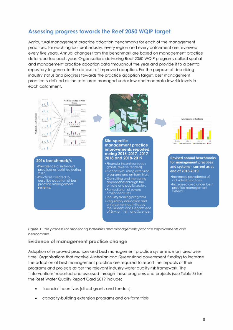
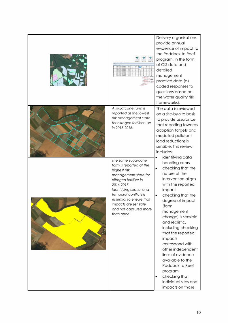
Delivery organisations

provide annual

evidence of impact to

the Paddock to Reef

program, in the form

of GIS data and

detailed

management

practice data (as

coded responses to

questions based on

the water quality risk

frameworks).

A sugarcane farm is

reported at the lowest

risk management state

for nitrogen fertiliser use

in 2015-2016.

The data is reviewed

on a site-by-site basis

to provide assurance

that reporting towards

adoption targets and

modelled pollutant

load reductions is

sensible. This review

includes:

identifying data

handling errors

checking that the

nature of the

intervention aligns

with the reported

impact

checking that the

degree of impact

(farm

management

change) is sensible

and realistic,

including checking

that the reported

impacts

correspond with

other independent

lines of evidence

available to the

Paddock to Reef

program

checking that

individual sites and

impacts on those

The same sugarcane

farm is reported at the

highest risk

management state for

nitrogen fertiliser in

2016-2017.

Identifying spatial and

temporal conflicts is

essential to ensure that

impacts are sensible

and not captured more

than once.

11

sites have not

previously been

reported to the

Paddock to Reef

program and

included in

estimates of

progress towards

the Reef 2050

WQIP targets.

For every site (usually

a paddock or farm),

the management

regime and how it is

has changed is

aligned to modelling

simulations which best

represent that

management (as

‘before’ and ‘after’

simulations). The

example (left) codifies

the trash

management,

machinery traffic and

tillage regime, nutrient

rates and timing, and

weed management

on a sugarcane farm.

Data provided

annually to Paddock

to Reef catchment

modelling constitutes

layers that describe

change in this way for

many hundreds of

individual sites.

The management

practice and

management system

baselines for each

catchment and

Natural Resource

Management (NRM)

region are adjusted

annually to reflect the

areas validated in the

above steps.

12

Reef Water Quality

Report Cards contain

data aggregated up

to represent estimates

of area under

management systems,

at the scale of NRM

regions.

Figure 2: The broad process for evaluating impacts reported by organisations through the Reef 2050

WQIP.

13

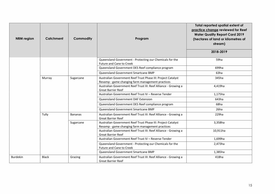
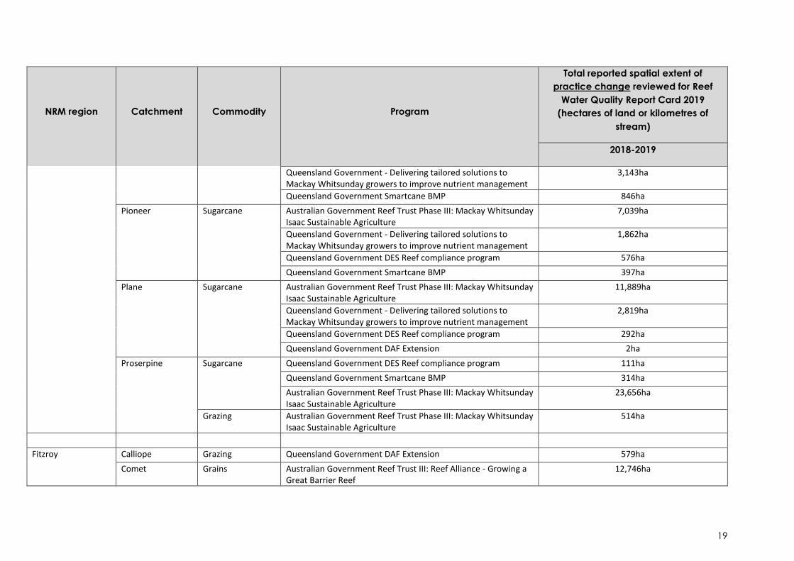
Table 3: Program and project investments reviewed for Reef Water Quality Report Card 2019

NRM region Catchment Commodity Program

Total reported spatial extent of

practice change reviewed for Reef

Water Quality Report Card 2019

(hectares of land or kilometres of

stream)

2018-2019

Cape York

Normanby

Bananas Australian Government Reef Trust III: Reef Alliance - Growing a Great Barrier Reef

146ha

Grazing

Australian Government Reef Trust Phase II: Fifty percent reduction in gully erosion from high priority sub-catchments in the Normanby

332ha

Australian Government Reef Trust Phase IV: Laura Gullies Project, fix up and skills for the future

7,770ha

Wet Tropics Barron


13ha

Grains Australian Government Reef Trust III: Reef Alliance - Growing a Great Barrier Reef

388ha

Sugarcane

Australian Government Reef Trust Phase III: Project Catalyst Revamp - game changing farm management practices

384ha

Australian Government Reef Trust III: Reef Alliance - Growing a Great Barrier Reef

1,695ha

Australian Government Reef Trust IV – Reverse Tender 376ha

Daintree

Sugarcane Australian Government Reef Trust Phase III: Project Catalyst Revamp - game changing farm management practices

11ha


586ha

Herbert

Grazing Australian Government Reef Trust Phase IV: Improving Reef Water Quality through Herbert River Catchment and Gully

8,763ha


5,584ha

14






stream)

2018-2019


29,608ha

Australian Government Reef Trust IV – Reverse Tender 2,183ha

Queensland Government DAF Extension 9ha

Queensland Government DES Reef compliance program 823ha

Johnstone Bananas Australian Government Reef Trust III: Reef Alliance - Growing a Great Barrier Reef

473ha


1,658ha


14,976ha


Queensland Government - Protecting our Chemicals for the Future and Cane to Creek

353ha


Queensland Government Smartcane BMP 684ha

Mossman Sugarcane Australian Government Reef Trust Phase III: Project Catalyst Revamp - game changing farm management practices

2,089ha


5,134ha



Mulgrave-Russell Sugarcane Australian Government Reef Trust III: Reef Alliance - Growing a Great Barrier Reef

6,763ha

Australian Government Reef Trust IV – Reverse Tender 606ha


15






stream)

2018-2019


59ha



Murray


345ha


4,419ha





Tully


229ha


3,358ha


10,911ha



2,473ha

Queensland Government Smartcane BMP 1,385ha

Burdekin

Black Grazing Australian Government Reef Trust III: Reef Alliance - Growing a Great Barrier Reef

418ha

16






stream)

2018-2019

Bowen

Grazing

Australian Government Reef Trust Phase II: Point Source Sediment Management in the Burdekin Dry Tropics NRM Region - Bowen Bogie

105ha


16,555ha


8.1km

Australian Government Reef Trust Phase IV: Stomping out Sediment in the Burdekin - livestock impact for gully remediation

869ha

Queensland Government - Burdekin Major Integrated Project 6,159ha

Queensland Government DAF Extension 37,911ha

Don

Grazing


32,513ha


35.4km


Horticulture Queensland Government - Hort360 GBR BMP 71ha

Haughton

Grazing

Australian Government Reef Trust Phase I: Promotion of A-class Grazing

129ha


4,039ha


8.4km

Sugarcane Australian Government Reef Trust III: Reef Alliance - Growing a Great Barrier Reef

3,490ha


17






stream)

2018-2019

Queensland Government - Engaging Burdekin Sugarcane Farmers for Improved Water Quality Outcomes

147ha

Queensland Government RP161 Complete Nutrient Management Planning for Cane Farming

2,727ha

Lower Burdekin Grazing Australian Government Reef Trust Phase I: Promotion of A-class Grazing

4,827ha

Lower Burdekin Grazing

Australian Government Reef Trust Phase II: Point Source Sediment Management in the Burdekin Dry Tropics NRM region - East Burdekin

538ha


14,995ha


55.2km

Australian Government Reef Trust Phase IV: Gully restoration in priority reaches to improve water quality on the Great Barrier Reef - Lower Burdekin (Greening Australia)

56ha

Australian Government Reef Trust Phase IV: Stomping out Sediment in the Burdekin - livestock impact for gully remediation

21ha

Queensland Government - Burdekin Major Integrated Project 182ha

Queensland Government - Innovative gully remediation (Greening Australia) - erosion management plan and operational works on Strathalbyn Station.

52ha



Sugarcane Queensland Government DES Reef compliance program 3,566ha

18






stream)

2018-2019


4,308ha


Queensland Government - Engaging Burdekin Sugarcane Farmers for Improved Water Quality Outcomes

24ha

Queensland Government RP161 Complete Nutrient Management Planning for Cane Farming

1,626ha

Suttor


5,629ha

Grazing


57,106ha


9.3km


Upper Burdekin

Grazing

Australian Government Reef Trust Phase I: Promotion of A-class Grazing

1,765ha


133,083ha


94km


Mackay Whitsunday O’Connell Grazing Australian Government Reef Trust Phase III: Mackay Whitsunday Isaac Sustainable Agriculture

1,464ha


Sugarcane Australian Government Reef Trust Phase III: Mackay Whitsunday Isaac Sustainable Agriculture

11,676ha

19






stream)

2018-2019

Queensland Government - Delivering tailored solutions to Mackay Whitsunday growers to improve nutrient management

3,143ha


Pioneer Sugarcane Australian Government Reef Trust Phase III: Mackay Whitsunday Isaac Sustainable Agriculture

7,039ha


1,862ha



Plane Sugarcane Australian Government Reef Trust Phase III: Mackay Whitsunday Isaac Sustainable Agriculture

11,889ha


2,819ha



Proserpine Sugarcane



Australian Government Reef Trust Phase III: Mackay Whitsunday Isaac Sustainable Agriculture

23,656ha

Grazing Australian Government Reef Trust Phase III: Mackay Whitsunday Isaac Sustainable Agriculture

514ha

Fitzroy

Calliope Grazing Queensland Government DAF Extension 579ha

Comet


12,746ha

20






stream)

2018-2019

Grazing


4,258ha


Dawson


18,987ha

Grazing


49,813ha


138.4km


Isaac


5,125ha

Grazing Australian Government Reef Trust Phase II: Gully Remediation in the Fitzroy by Revegetation and Grazing Land Management

26ha


18,330ha


7.6km


Lower Fitzroy

Grazing

Australian Government Reef Trust Phase II: Gully Remediation in the Fitzroy by Revegetation and Grazing Land Management

336ha


1.7km


7,847ha


21km

21






stream)

2018-2019

Australian Government Reef Trust Phase IV: F11 Fitzroy sub-catchment gully and stream bank erosion control program

130ha



Mackenzie


3,086ha

Grazing Australian Government Reef Trust Phase II: Gully Remediation in the Fitzroy by Revegetation and Grazing Land Management

1,459ha


4km


11,611ha


24km


Nogoa


16,454ha

Grazing Australian Government Reef Trust III: Reef Alliance - Growing a Great Barrier Reef

5,512ha


3km

Nogoa Grazing Queensland Government DAF Extension 27,698ha

Styx

Grazing


74ha


464ha

22






stream)

2018-2019


0.5km

Waterpark Grazing Queensland Government DAF Extension 13ha

Burnett Mary Baffle


2,317ha


6.3km

Burnett Grains Australian Government Reef Trust III: Reef Alliance - Growing a Great Barrier Reef

1,337ha

Grazing


2,428ha


3.3km

Horticulture Australian Government Reef Trust III: Reef Alliance - Growing a Great Barrier Reef

188ha

Queensland Government - Hort360 GBR BMP 152ha


262ha

Burrum


64ha



3,270ha

Kolan

Horticulture


59ha


23






stream)

2018-2019


55ha

Mary

Grazing

Australian Government Reef Trust Phase II: Gully management in highly erodible sub-catchments of the Mary River Catchment

173ha


1,664ha


8.7km

Australian Government Reef Trust Phase IV : Great Barrier Reef Riparian Zone Management - a Mary River Project

150ha

Australian Government Reef Trust Phase IV : Great Barrier Reef Riparian Zone Management - a Mary River Project

7.1km


105ha

Sugarcane Queensland Government Smartcane BMP 275ha

24

Describing progress

Management practices that are at the moderate-low risk and low risk levels are considered as

‘best management practices’. These are summed when describing the proportion of the total

area in a catchment that is managed under best practice, and practices are combined

according to their weightings to describe ‘best management practice systems’. Colour coding

based on five categories (see Table 4) is also used to indicate progress toward the 90 per cent

adoption target.

Table 4: Colour-coded scoring system used to indicate progress

Qualitative confidence rankings

Sugarcane Grazing Horticulture Grains Bananas

A multi-criteria analysis has been used to qualitatively score the confidence in each indicator

used in the Reef Water Quality Report Card from low to high. The approach combined expert

opinion and direct measures of error for program components where available.

References

Australian and Queensland governments 2018, Reef 2050 Water Quality Improvement Plan

2017-2022. https://www.reefplan.qld.gov.au/about/

Further reading

McCosker K, Northey A (2015). Paddock to reef: Measuring the effectiveness of large scale

investments in farm management change. Rural Extension & Innovation Systems Journal,

vol.11, 177-184.

Adoption progress – scoring system

0–22% E – Red Very poor

23–45% D – Orange Poor

46–67% C – Yellow Moderate

68–89% B – Light green Good

90–100 % A – Dark green Very good

https://www.reefplan.qld.gov.au/about/

25

Glossary

Adoption: Adoption in this context is the process of changing how something is done on farms.

Adopting a new farm management practice usually requires the acquisition of new

knowledge and skills, and often new or different farm equipment and infrastructure. The extent

to which a specific practice is adopted (adoption rate) is described as a percentage of the

overall population or area. For example, 98% of the sugarcane growing area in the Johnstone

catchment retains harvested crop residues on the soil surface.

Benchmark: a value set at a reference point in time. In this context, benchmarks are describing

farm practice adoption rates at specific points in time. For example, the 2016 benchmark for

low-risk usage regime of residual herbicides in sugarcane in the Burdekin catchment is 67% of

the sugarcane growing area.

Best management practice systems: farms are managed using many different management

practices. There is a ’best practice’ level for each of these practices. The farm management

system is a complex blend of all of these practices. Achieving a best management practice

system means that all, or the majority of the constituent practices, are occurring at the best

practice level. In the context of the Reef 2050 WQIP, the management systems described are

best practice for off-farm water quality.

Industry Best Management Practice (BMP) Program: Many agricultural industry sectors lead a

voluntary program that assists landholders to benchmark their current practices against an

industry-developed set of standards. These standards are available for all aspects of farm

business management, including the many of elements that are relevant when considering

risks to off-farm water quality. Industry BMP programs operating in Great Barrier Reef

catchments during 2018-2019 included:

Sugarcane: Smartcane BMP (Queensland Cane Growers Organisation)

Bananas: Banana BMP Guide (Australian Banana Growers’ Council)

Horticulture: Hort360 (Growcom)

Stewardship: Stewardship is the responsibility of carefully managing something. In the context

of the Reef 2050 WQIP, it involves implementing or supporting farm practices that reduce

sediment, nutrient and pesticide pollution.

26

Ground cover monitoring methods

This report summarises the data and methods used for reporting progress towards the Reef

2050 Water Quality Improvement Plan (Reef 2050 WQIP) (Australian and Queensland

governments 2018) 2025 land and catchment management target for ground cover.

The target for ground cover is:

90% of grazing lands will have greater than 70% ground cover in the late dry season.

“The ground cover target focusses on late dry season ground cover levels across grazing lands,

recognising that water quality risk is generally highest at the onset of the wet season. The target

incorporates an area-based component (i.e. 90% of grazing lands will have achieved the

ground cover target), while providing for natural variability in ground cover levels. Research

supports a ground cover target of 70% to minimise erosion.”(Reef 2050 WQIP)

Background

Why measure ground cover?

Ground cover is defined as the vegetation (living and dead) and biological crusts and rocks

that are in contact with the soil surface and is a key indicator of catchment condition. Ground

cover is a key component of many soil processes including infiltration, run-off and surface

erosion. In the Great Barrier Reef catchments, low ground cover can lead to soil erosion which

contributes to increased sediment loads reaching the Great Barrier Reef lagoon and loss of

productivity for grazing enterprises.

It is particularly important to maintain ground cover during dry periods, or periods of unreliable

rainfall, to minimise loss of water, soil and nutrients when rainfall eventually occurs. This practice

will also maximise the pasture growth response to rainfall. Implementing appropriate and

sustainable land management practices, particularly careful management of grazing pressure,

can help to maintain or improve ground cover, reducing erosion and improving the stability

and resilience of the grazing system.

Factors that influence ground cover

Ground cover levels are the result of complex interactions between landscape function (soil

type, topography and vegetation dynamics), climate and land management. Some areas

maintain naturally higher levels of ground cover due to factors such as high soil fertility and

consistently high annual rainfall. The impacts of grazing land management practices on

ground cover levels in these areas can be minimal due to the resilience of the land in

responding to pressures. In areas where rainfall is less reliable and soils are less fertile, ground

cover levels can vary greatly and the influence of grazing land management practices on

ground cover levels, and on the species composition of the ground cover, can be more

pronounced.

A number of initiatives aimed at improving grazing land management in Great Barrier Reef

regions are in place or are planned. They include programs which are improving management

of ground cover levels appropriate to the regional conditions such as:

the Grazing Resilience and Sustainable Solutions (GRASS) program provides one-on-one

support to help graziers improve poor and degraded land

27

infrastructure projects such as fencing key areas and better distribution of watering

points for stock

trials of different grazing strategies

a range of extension and education activities including development of online,

interactive and reporting tools for accessing and viewing ground cover information.

Reporting ground cover levels for the Reef 2050 Water Quality Improvement

Plan

Progress towards the 2025 land and catchment management ground cover target is assessed

by the Queensland Ground Cover Monitoring Program. It is based on the measurement of late

dry season ground cover using Landsat satellite imagery for historical measurements and

Sentinel-2 satellite imagery, when available, in more recent years (post-2015). All imagery has

been processed to produce fractional ground cover estimates, using field data for calibration.

While a range of factors influence ground cover levels at local scales, reporting is focused only

on information that describes regional ground cover levels in the current and historical context.

Rainfall data is provided for context only, as it is the primary driver of ground cover levels at a

regional scale.

A range of products have been developed by the Queensland Ground Cover Monitoring

Program that account for the influence of climate, land management and soil type. These

products are more appropriate for monitoring local-scale variability and differences in ground

cover levels and are of limited use for regional-scale reporting. Access to some of these

products is via the interactive online tool VegMachine and the online reporting tool, FORAGE.

Products that prove useful for describing ground cover levels at the regional scale will help to

revise future ecologically-relevant and regionally-focused targets, and will be incorporated

into future reporting.

Methods

Ground cover data

Satellite imagery and fractional ground cover

Measurement of ground cover for reporting is based on fractional ground cover data derived

following methods described in Scarth et al. (2010), Guerschman et al. (2015) and Trevithick et

al. (2014). The fractional ground cover method measures the proportion of green cover, non-

green cover and bare ground using reflectance information from late dry season from several

sources of satellite imagery. This includes the longer-term dataset of Landsat imagery (1987 to

present): Landsat 5 Thematic Mapper, Landsat 7 Enhanced Thematic Mapper and Landsat 8

Operational Land Imager satellites with a spatial resolution of approximately 30m and an

acquisition frequency of 16 days. In more recent years (mid-2015 to present), the European

Space Agency’s Sentinel-2A and Sentinel-2B satellites have augmented the Landsat record.

These satellite sensors have a spatial resolution of 10m and an acquisition frequency of five

days. Analyses undertaken by Flood (2017) has shown that fractional cover data produced

from the two imagery sources is statistically comparable as the surface reflectance values of

the Sentinel-2 products have been adjusted to closely match those from the Landsat satellites.

The inclusion of the Sentinel-2 data is expected to improve ground cover estimates, particularly

in areas that are cloud affected, due to the more frequent acquisition strategy. For all

reporting, the Sentinel-2 data are downscaled (i.e. degraded) to 30m to match the spatial

resolution of the Landsat data.

http://vegmachine.net/

https://www.longpaddock.qld.gov.au/forage/

28

It is important to note that the fractional cover data measures all cover as viewed from above

by the satellite, including the trees and shrubs as well as the ground cover and bare ground. To

derive a ground cover estimate, a further step is applied following Trevithick et al. (2014) which

uses another remote sensing product, called the ‘persistent green’, to effectively remove the

influence of trees and shrubs on the fractional cover data. The persistent green product is

based on a time-series of imagery and an analysis of the behaviour of the green cover fraction

over that time-series. The assumption with this product is that the minimum of the time-series

represents the less seasonally-variable woody vegetation, effectively providing an estimate of

the level of woody cover at any given (pixel) location. This estimate is then converted to a

measure of the gap fraction of the woody vegetation, which is basically a measure of the

amount of gaps or spaces in the tree and shrub layer(s) when viewed vertically from above (or

below). A relationship is then defined, based on quantitative field data estimates of overstorey

and ground cover data and gap fractions, which estimates the amount of ground cover and

bare ground that is expected given a particular overstorey gap fraction estimate. An

adjustment is then made to the fractional cover to provide individual (i.e. pixel-level) estimates

of the level of green ground cover, non-green ground cover and bare ground at ground level,

thus producing a fractional ground cover estimate (Figure 1). As a final step, the green and the

non-green ground cover fractions are summed to produce a total ground cover estimate, as

erosion and run-off are influenced by all ground cover. This estimate of total ground cover is

used for reporting and is hereafter referred to simply as ‘ground cover’.

Figure 3: Schematic representation of the correction of the fractional cover data to estimate the

fractional ground cover used for reporting (Trevithick et al., 2014). (a) Fractional cover measures all

vegetation cover including trees, shrubs and ground cover, as well as bare ground. The ground cover

and bare ground are partially obscured by the trees and shrubs. (b) Next, a time-series approach is used

to estimate the percentage of ‘persistent green’ cover in the tree and shrub layers. (c) Finally, a

correction factor is applied, based on field data, to effectively remove the ‘persistent green’ cover in the

tree and shrub layers, thus providing an estimate of the green cover, non-green cover and bare ground,

all at the ground level – the fractional ground cover or simply ‘ground cover’.

29

The method for deriving ground cover can be applied in areas of woody vegetation cover up

to approximately 60% persistent green cover, at which point the canopy becomes too dense

to reliably achieve an estimate of the ground cover. Given the low levels of woody vegetation

cover in the Great Barrier Reef catchment areas, this means that generally, ground cover can

be reported for the majority (i.e. >90%) of the grazing lands.

The use of the persistent green product to derive ground cover does have some limitations.

Given it is an estimate of green cover behaviour over time, some non-woody areas which are

persistently green (e.g. in high rainfall areas), can have very high persistent green cover values

(i.e. >60%), resulting in them not being included in the areas for analysis and reporting. Further,

due to the way the persistent green product is derived using time-series approaches, it can

only be calculated up to a date which is two years prior to the current (reporting) season. As a

result of these limitations, ground cover reporting statistics calculated in one reporting period

may vary slightly when re-calculated and updated in the next reporting period, as will the area

of the grazing lands actually analysed and reported. In general, the reporting of mean cover

helps to account for these differences. Future work will consider ways to further limit the impact

these issues have on the ongoing consistency of the ground cover reporting.

The current version of the fractional ground cover product was developed using around 2000

field observations across a range of ground cover, tree cover and shrub cover levels within a

range of environments (Scarth et al., 2010; Guerschman et al., 2015). It has been assessed using

linear regression to have an accuracy of 17% Root Mean Square Error (Figure 2). Due to a

collaborative national effort, there are now over 4000 field observations collected using the

same field protocols across Australia, and a re-calibrated and revised fractional cover model is

being developed. It is expected that this updated version will help to address some known

limitations in the current version (e.g. in bright soil areas) and will be incorporated into reporting

in the future, following assessment of the accuracy and degree of difference to the current

reporting. Re-processing of previous years will be undertaken to produce reporting statistics

which are based on a single, consistent product.

Figure 2: Comparison of field measurements of fractional cover with Landsat derived fractional ground

cover for 2047 sites across Australia. The linear regression shows an overall RMSE of 17%.

17 % RMSE

Slope = 1.097

R2 = .63

30

Late dry season ground cover

Late dry season ground cover is defined using seasonal composites of images for spring

(September–November) (for the period 1987 to present). It is estimated using a seasonal

composite of fractional ground cover data images (Landsat prior to 2015 and Sentinel-2 post-

2015) acquired throughout the season following Flood (2013). This approach has the

advantage of removing errors and outliers in the data (e.g. due to cloud or cloud shadow

artefacts) and produces a composite image for the season which is based on the selection,

per pixel, of the most representative value for that season. Each pixel is a real estimate

selected from the set of images available for that season; it is not a modelled or synthesised

value. The method requires at least three valid observations in any given season before a pixel

is selected for inclusion in the composite image. It provides the most spatially comprehensive

coverage as there is generally very little missing data due to cloud, cloud shadow or satellite

sensor issues. For areas where there is still missing data, further infilling can be undertaken using

what are referred to as seasonal ground cover ‘patches’. These are pixel values generated in

areas where less than three valid observations were made in a season. This process is only

undertaken for the Landsat imagery, as the more frequent acquisition strategy of the Sentinel-2

satellites typically results in very little missing data once composited.

Reporting regions and grazing lands

Reporting is based on the six natural resource management regions of the Great Barrier Reef

region:

Cape York

Wet Tropics

Burdekin

Mackay Whitsunday

Fitzroy

Burnett Mary.

Grazing lands in the reporting regions are spatially-defined based on the most recent land use

data provided by the Queensland Land Use Mapping Program (DSITIA, 2012). The most recent

version of the mapping for Burdekin and Wet Tropics is 2016, with the Fitzroy and Burnett Mary

current to 2017. Cape York and the Wet Tropics are current to 2013 and 2015, respectively.

A reporting region is defined as that part of a region which is grazing land and has less than

approximately 60% persistent green cover. Any reporting region with less than 10% area

reported as grazing lands, or less than 10% ground cover data within the grazing lands, is

excluded from the results.

Reporting ground cover

This report provides a regional overview of late dry season ground cover levels in the Great

Barrier Reef catchments based on analysis of seasonal (i.e. spring) ground cover data. The

statistics are calculated for each pixel (i.e. 30m x 30m area) and then summarised (i.e.

averaged) for each of the 35 catchments.

Statistics reported include mean late dry season ground cover from 1987 to the current

reporting period, and the percentage of the region’s reported grazing area with late dry

season ground cover greater than 70% in the current reporting year. Graphs show the mean

31

ground cover levels over time, with rainfall included to provide context. Maps of ground cover

percentages are also provided for the entire Great Barrier Reef region, and for each reporting

region, to show where in each region the ground cover levels were higher or lower.

It is important to note that averaging ground cover across whole regions can mask localised

areas of lower or higher cover, particularly in large catchments with a strong rainfall gradient

(e.g. the Burdekin and Fitzroy). The mean ground cover reported is, therefore, indicative of

general levels of ground cover within the reporting region. Reporting is further divided into

catchments (and sub-catchments for larger catchments). For more detailed or localised

ground cover information and to visualise ground cover data products, refer to VegMachine

or FORAGE.

Rainfall data

Rainfall data is provided for current and historical context as rainfall is the primary driver of

ground cover levels at the regional scale. In general, high rainfall in the preceding seasons

results in higher ground cover levels and low rainfall results in lower ground cover levels. Rainfall

data is obtained from SILO as a 5km grid. The mean annual rainfall is then calculated for each

reporting region from September to August for each year from 1986, to align the mean annual

rainfall with the late dry season reporting period. It should be noted that rainfall statistics are

constantly updated by the Bureau of Meteorology as more data becomes available, thus

reported mean annual rainfall may change slightly between reporting periods.

Scoring system

A standardised scoring system is used for each of the key indicators in the reef report card. The

scoring system is used to assess and communicate the status of the indicator against the Reef

2050 WQIP 2025 targets.

Ground cover target

1. 90% of grazing lands will have greater than 70 per cent ground cover in the late dry season.

Table 1: The colour-coded ground cover scoring system

Status Criteria Grade and

colour code

Very poor ground cover Less than 60% of grazing lands meet the

adequate ground cover level

E - Red

Poor ground cover Between 60-69% of grazing lands meet the


D - Orange

Moderate ground cover Between 70-79% of grazing lands meet the


C - Yellow

Good ground cover Between 80-89% of grazing lands meet the


B - Light Green

Very good ground

cover – Target met

More than 90% of grazing lands meet the


A - Dark Green

Adequate ground cover for 2019 is defined as >70% late dry season ground cover.

http://vegmachine.net/

https://www.longpaddock.qld.gov.au/forage/

https://www.longpaddock.qld.gov.au/silo/

https://www.reefplan.qld.gov.au/tracking-progress/reef-report-card/scoring-system

https://www.reefplan.qld.gov.au/

https://www.reefplan.qld.gov.au/

32

Qualitative confidence ranking

A multi-criteria analysis is used to qualitatively score the confidence in each indicator used in

the Reef report card from low to high. The approach combined the use of expert opinion and

direct measures of error for program components where available. Ground cover has received

a four-bar confidence ranking. Groundcover

Maturity of

methodology

(weighting 0.5)

Validation Representativeness Directness Measured

error

New or

experimental

methodology

Remote sensed data

with no or limited

ground truthing

1:1,000,000

Measurement of

data that have

conceptual

relationship to

reported indicator

Error not

measured

or >25%

error

Peer reviewed

method

Remote sensed data

with regular ground

truthing (not

comprehensive)

1:100,000 Measurement of

data that have a

quantifiable

relationship to

reported indicators

10-25% error

Established

methodology in

published paper

Remote sensed data

with comprehensive

validation program

supporting (statistical

error measured)

1:10,000

Direct measurement

of reported indicator

with error

Less than

10% error

3 x0.5 = 1.5 3 3 2 2 Bolded cells indicate assessment ranking

Total score = 11.5, equates to four dots.

References

Australian and Queensland governments 2018, Reef 2050 Water Quality Improvement Plan

2017-2022, State of Queensland, Brisbane

Department of Science, Information Technology, Innovation and the Arts 2012, Land use

summary 1999-2009: Great Barrier Reef catchments, Queensland Department of Science,

Information Technology, Innovation and the Arts, Brisbane.

Flood, N 2017, ‘Comparing Sentinel-2A and Landsat 7 and 8 Using Surface Reflectance over

Australia’, Remote Sensing, vol. 9, no. 659.

Flood, N 2013, ‘Seasonal composite Landsat TM/ETM+ images using the medoid (a multi-

dimensional median)’, Remote Sensing, vol. 5, no. 12, pp. 6481–6500.

Guerschman J, Scarth P, McVicar T, Renzullo L, Malthus T, Stewart J, Rickards J & Trevithick R

2015, ‘Assessing the effects of site heterogeneity and soil properties when unmixing

photosynthetic vegetation, non-photosynthetic vegetation and bare soil fractions from

Landsat and MODIS data’, Remote Sensing of Environment, vol. 161, pp. 12–26.

Scarth P, Roder A & Schmidt M 2010, ‘Tracking grazing pressure and climate interaction – the

role of Landsat fractional cover in time series analysis’ in Proceedings of the 15th Australasian

Remote Sensing and Photogrammetry Conference, Alice Springs, Australia, pp. 13–17.

Trevithick, R, Scarth, P, Tindall, D, Denham, R & Flood, N 2014, Cover under trees: RP64G

Synthesis Report, Queensland Department of Science, Information Technology, Innovation and

the Arts, Brisbane. <https://publications.qld.gov.au/dataset/ground-cover-fire-grazing>

https://publications.qld.gov.au/dataset/ground-cover-fire-grazing

33

Catchment pollutant delivery – Catchment loads

modelling methods

This report summarises the data and methods used for reporting progress toward the Reef 2050

Water Quality Improvement Plan (Reef 2050 WQIP) (Australian and Queensland governments

2018) 2025 water quality targets. The catchment loads modelling program is one line of

evidence used to report on progress in the Reef Water Quality Report Card 2019.

The water quality targets are:

60% reduction in anthropogenic end-of-catchment dissolved inorganic nitrogen loads

20% reduction in anthropogenic end-of-catchment particulate nutrient loads

25% reduction in anthropogenic end-of-catchment fine sediment loads

pesticides: to protect at least 99% of aquatic species at the end-of-catchments.

Catchment loads modelling

Quantifying the impact of land management practice change on long-term water quality

through monitoring alone is not possible at the whole Great Barrier Reef (GBR) scale. Models

are, therefore, used in conjunction with the monitoring program to predict long-term changes

in water quality.

The purpose of the modelling is to report annually on the progress towards the Reef 2050 WQIP

2025 load reduction targets for total suspended sediment (TSS), dissolved inorganic nitrogen

(DIN), particulate phosphorus (PP) and particulate nitrogen (PN).

The ability to model progress towards the new pesticide target is continuing to be developed.

In the meantime, pesticide risk is reported through the catchment loads monitoring program.

The eWater Source Catchments modelling framework (eWater, 2010) was modified to GBR

Source (Ellis 2017) to enable the synthesis of management practice change, paddock

monitoring and modelling, and catchment monitoring data to estimate end-of-catchment

pollutant loads. The catchment models generate pollutant loads for current and improved

practices for each individual land-use. Modelling is conducted over a fixed climate period. This

enables changes in water quality that are only due to the implementation of improved

management practices to be modelled.

Baseline loads are estimated for the current management practice benchmark (2016).

From the baseline, the reduction in loads resulting from improved management practice

adoption is calculated by running the model with the new practice adoption layer for the

same 28-year modelling period as the baseline. The difference in load is the load reduction for

that investment year.

Pollutant loads are summarised in the report card for the 35 basins draining to the Great Barrier

Reef lagoon. This catchment-scale water quantity and quality model uses a node link network

to represent processes of generation, transportation and transformation of water and

constituents within major waterways in a catchment (see Figure 1). The model generates

estimates of run-off and pollutant loads for each functional unit (FUs - areas within a sub-

catchment that have similar behaviour in terms of run-off generation and/or nutrient

generation, e.g. land use) within a sub-catchment. Run-off and pollutants are transported from

34

a sub-catchment through the stream network, represented by nodes and links, to the end of

the catchment. These components represent the sub-catchment and waterway network.

Figure 4: Example of a functional unit (FU) and node-link network generated in Source Catchments

(source eWater).

The Source Catchment model runs at a daily time-step which enables the interactions of

climate and land management to be reflected in modelled outputs. Aggregated average

annual catchment loads are required for the report card. The model runs for a fixed climate

period (1986 to 2014), to remove the influence of climate on estimated load reductions. The

most current land-use mapping is incorporated when models are periodically updated (details

of the mapping data can be found at:

www.qld.gov.au/environment/land/management/mapping/statewide-monitoring/qlump/qlump-datasets).

The pollutants modelled were:

fine sediment (TSS) and coarse sediment

dissolved and particulate nutrients.

The Paddock to Reef Integrated Monitoring, Modelling and Reporting Program (Paddock to

Reef program) agricultural management practice adoption program has developed water

quality risk frameworks for each agricultural industry. These frameworks articulate best

management practice in relation to the Reef 2050 WQIP land and catchment management

targets for agricultural management practice adoption. These practices are described in terms

of their relative water quality risk, from low to high. See the Agricultural land management

practice adoption methods (Australian and Queensland governments, 2019b) report for more

information about the water quality risk frameworks.

Representation of pre-agricultural land management scenario

It is important to note that the pre-development modelled loads were constructed to reflect a

scenario prior to agricultural development. The aim was to enable load changes from

management to be quantified. The scenario does not represent a true pre-development

landscape. Off-shore coral coring and sediment tracing work suggests anthropogenic loads

have increased anywhere from 2-10 times the current load (Bartley et al. 2018, Lewis et al 2014

35

and Hughes et al 2009, McCulloch et al 2003a). The modelled estimates of fine sediment fall

within these ranges.

The assumptions made when modelling pre-development are:

Hydrology was kept the same for baseline and the pre-agricultural land management

scenarios with dams and weirs maintained.

Ground cover was increased to 95% in grazing areas.

With the exception of grazing, all other land uses reverted to nature conservation area.

The foliage projected cover layer was increased to 95% riparian cover.

Gully cross-section areas were reduced to 10% of their baseline values.

Management factors for streambank models were adjusted to reflect a very low risk to

water quality.

To reflect the modelled load reduction for each report card as a result of changes in adoption

of improved agricultural management practices, three scenarios1 are run:

pre-development load (prior to agricultural development) for the 28-year modelling

period

the baseline load for the 28-year modelling period (i.e. representing the agricultural

management practice benchmark 2016)

change load for the 28-year modelling period with the proportion of land managed

using improved practices adjusted to reflect the previous year’s adoption.

The proportion of land managed using defined management practices is the only variable

that changes between modelled scenarios. This allows for the relative load reductions

attributed to the areas of improved agricultural management practices to be reported.

Approximately 10 land uses are modelled in each region including grazing, sugarcane, grain

cropping, horticulture and bananas.

Modelled load estimates were calibrated and or validated against field data collected

through the Catchment Loads Monitoring program at 43 monitoring sites across 20 catchments

that discharge to the Great Barrier Reef lagoon. For further information on the model

calibration and validation processes and results, refer to McCloskey et al. 2017A and Waters et

al 2014.

The Catchment Loads Modelling program undergoes an external peer review every three to

four years. The program was reviewed in 2012, 2015 and 2019. Prior to the release of each

report card, modelled load estimates are reviewed both internally and externally.

1 A scenario describes the major processes in a river system or catchment that are modelled. This includes catchment

and sub-catchment definition, rainfall run-off and constituent generation models, data sets and parameters. You can

create multiple scenarios to break complex projects into distinct parts or duplicate existing scenarios to conduct what-

if experiments without disrupting the original. Any change to the definition of sub-catchments, node-link network, FUs,

or the models within FUs, forms a new scenario. Similarly, a different set of inputs or parameters can be used to set up a

new scenario, such as a change in land use or a climate change (eWater Source User Guide 4.1).

https://www.reefplan.qld.gov.au/tracking-progress/paddock-to-reef/modelling-and-monitoring

36

Management practice change

The Reef 2050 WQIP water quality risk frameworks describe and categorise farming practices

according to recognised water quality improvements at the paddock scale. Improvements in

water quality as a result of adopting improved management practices were determined by

linking paddock model timeseries outputs to catchment models.

Management practice change has been modelled for the sugarcane, grains, horticulture,

banana and grazing areas of the Great Barrier Reef catchments. For details on how

management practice changes are represented in the modelling, refer to McCloskey et al.

2017A and Waters et al 2014.

Improved management of gullies and streambanks are modelled to reflect activities such as

gully restoration, excluding stock via fencing off gullies and streambanks, and installing off-

stream watering points. Spatial data on investments in improved practices are provided by

industry and the six natural resource management (NRM) bodies within each region to enable

good spatial representation of where works occurred.

Modelling assumptions

Loads reported for each report card reflect the relative change in modelled average

annual loads for the specified model run period (1986 to 2014).

Land use areas in the model are static over the model run period and are based on the

latest available Queensland Land Use Mapping Program (QLUMP) data.

Paddock model runs that are used to populate the catchment models represent

‘typical’ management practices for a given management class and do not reflect the

actual array of management practices that occur year-to-year across the Great Barrier

Reef catchments.

Paddock model simulations represent the reported management practice adoption

water quality risk frameworks as a set suite of practices.

Application rates of pesticides and fertilisers that are used to populate the paddock

models are derived through consultation with relevant industry groups and regional

NRM bodies.

Management practice adoption areas represented in the model are applied at the

spatial scale of the data supplied by the delivery organisations and collated by the

Department of Agriculture and Fisheries (DAF) Paddock to Reef Agricultural

Management Practice Adoption program team annually.

The water quality benefits from adopting a management practice change are

assigned in the year that on-ground works were implemented, so time lags that may

occur in the system are not accounted for.

It is important to note that these modelled load reductions are based on improved land

management adoption data supplied by organisations that receive Australian and

Queensland government funding to increase the adoption of best management

practices. Results are, therefore, indicative of the likely long-term water quality response

due to adoption of improved land management practices for a given scenario, rather

than a measured reduction in load.

http://www.reefplan.qld.gov.au/measuring-success/paddock-to-reef/management-practices/

37

Linking paddock and catchment models

The eWater Source Catchments model (www.ewater.org.au) was modified to incorporate

hillslope constituent generation from the most appropriate paddock models for cropping,

sugarcane and sugarcane areas, and the Revised Universal Soil Loss Equation (RUSLE) for

grazing. Gully and streambank erosion and floodplain, channel and reservoir deposition

processes added to the model were based on the SedNet/ANNEX approach (Wilkinson et al.

2014). The modified framework is referred to as P2R Source. A detailed description can be

found in Ellis and Searle (2013) and Ellis (2017). The spatial and temporal representation of gully,

streambank and in-stream erosion processes were incorporated to better represent the erosion

processes observed in the summer-dominant rainfall areas of northern Australia.

Two approaches were used to represent improved land management practices in the Source

Catchments model depending on the land use of interest. In the first approach, for sugarcane,

bananas and cropping, the constituent time-series (e.g. load per day per unit area) for the

given land use was supplied from a paddock model. Unique combinations of climate, soil type

and defined management practices within each land use were identified and represented

spatially in the paddock model simulations used to inform the catchment models. For cropping

(grain cereal crops) and bananas, the HowLeaky model was used (Rattray et al. 2004). For

sugarcane modelling, the Agricultural Production Systems sIMulator (APSIM) (Holzworth et al.

2014) was used. For load reduction representation, the defined management practice for a

particular land use segment was altered between scenarios.

In the second approach, the RUSLE model was written into the Source Catchments model to

model hillslope soil erosion in grazing lands. The cover term (C-factor) in the model is

generated from remotely sensed ground cover satellite imagery seasonally (four scenes per

year). The paddock-scale model GRASP (McKeon et al. 1990) was used to provide scaling

algorithms for each scenario to account for changes in management in each identified land

type; for example, shifting areas from moderate risk to moderate–low risk. These scaling

algorithms were applied at the pixel scale to each ground cover satellite image for the

modelling period. This is applied according to a spatial representation of areas of defined

management practices as provided annually by regional NRM bodies. Calculations were

performed pixel by pixel, with results accumulated to a single land use representation in each

sub-catchment. All loads generated for each land use represented within a sub-catchment

were then aggregated at the sub-catchment scale and routed through the stream network.

Total load

The total baseline load is the load modelled within each Great Barrier Reef catchment using

the 2016 management practice benchmark. A pre-development land use map was also

developed and modelled. The model was then run for a 28-year period to establish an

average annual load for this period; the pre-development load. The anthropogenic load was

calculated as the total baseline load less the pre-development load.

Load reductions

To reflect investment in improved management practices since 2016, the model was then re-

run in each year for the same climate period using the proportions of lowest risk to high risk

management practice areas in that year. The relative change in pollutant loads from the

anthropogenic baseline after investment reflects the load reduction due to changes in

management practices (see Figure 2).

http://www.ewater.org.au/

38

Figure 2: Example of modelled pre-development and anthropogenic pollutant loads, and the load

reduction following investment in improved management practices.

Modelling improvements

In response to the independent external review of the program in 2015 and 2019, and

recommendations from the Queensland Audit Office and the Great Barrier Reef Water

Science Taskforce (GBRWST, 2016), improvements include:

A desktop and field gully mapping program continues to improve the spatial

representation of gully density and geometry in the models. Updated gully maps have

been incorporated for selected areas within the Fitzroy region.

Annual monitoring/modelling validation workshops are held to compare model

performance against monitoring data.

Updated land use mapping incorporated for the Fitzroy, Burdekin and Burnett Mary

regions.

Research into parameter sensitivity/uncertainty in modelled inputs and outputs is

continuing to guide future data collection and provide estimates of load uncertainty.

Baseline load

(Management Practice Benchmark

2016)

Post improved

practice adoption load

(e.g. 2017/2018)

Co

nst

itu

en

t lo

ad

Natural (pre-development) load

Anthropogenic load

50% Target

Load reduction

39

How the information is reported

Progress towards the targets is estimated by determining how much the modelled pollutant

load has reduced from the average annual modelled anthropogenic baseline (total load less

the pre-development load). This is calculated as a percentage reduction in average annual

modelled load.

Modelled TSS, DIN, PN and PP at the end of the catchment are reported for the total Great

Barrier Reef catchment, six regions and 35 sub-catchments.


Dissolved

inorganic

nitrogen

Particulate

nitrogen

Particulate

phosphorus

Sediment

A multi-criteria analysis was used to qualitatively score the confidence in each indicator used

in the report card, from low to high. The approach combined expert opinion and direct

measures of error for program components where available.

Sediment and particulate nutrients scored higher for confidence as the modelling for these

parameters is based on well established methods, particularly for hillslope erosion processes.

Models are validated with data from more than 43 catchment loads monitoring sites and

modelled relationships are based on published data from historic and ongoing research.

Extensive gully mapping underpins the sediment modelling. The models undergo numerous

quality assurance checks and research is currently underway to measure and report

uncertainty within the models.

Dissolved inorganic nitrogen scored lower for confidence as the way in which nitrogen

changes form as it moves from paddock to the Great Barrier Reef is more complex to represent

within the modelling framework.

The average annual percentage reduction in load is calculated as:

Reduction in load (%) = (anthropogenic baseline load – anthropogenic change) x 100

Anthropogenic baseline load

where, anthropogenic baseline load = total load less pre-development load

40

References

Australian and Queensland governments, 2019a, Catchment Pollutant Delivery - Catchment

Loads Monitoring Method Summary, Paddock to Reef Integrated Monitoring, Modelling and

Reporting program, Queensland Government, Brisbane, Australia.

Australian and Queensland governments, 2019b, Stewardship – Agricultural Management

Practice Adoption Methods, Paddock to Reef Integrated Monitoring, Modelling and Reporting

program, Queensland Government, Brisbane, Australia.

Australian Government and Queensland Government, 2018, Reef 2050 Water Quality

Improvement Plan 2017–2022, Queensland Government, Brisbane, Australia, pp. 56,

<www.reefplan.qld.gov.au/__data/assets/pdf_file/0017/46115/reef-2050-water-quality-

improvement-plan-2017-22.pdf>.

Queensland Land Use Mapping Program 2019, Queensland Department of Environment and

Science, Brisbane, Australia.

<www.qld.gov.au/environment/land/management/mapping/statewide-

monitoring/qlump/qlump-datasets>.

Bartley, R., Bainbridge, Z.T., Lewis, S.E., Kroon, F.J., Wilkinson, S.N., Brodie, J.E., Silburn, D.M.,

2014a. Relating sediment impacts on coral reefs to watershed sources, processes and

management: a review. Sci. Total Environ. 468–469C, 1138–1153.

Ellis, R & Searle, R 2013, ‘An integrated water quality modelling framework for reporting on

Great Barrier Reef catchments’, in J Piantadosi, RS Anderssen and J Boland (eds) MODSIM2013,

20th International Congress on Modelling and Simulation, Modelling and Simulation Society of

Australia and New Zealand, December 2013, pp. 3183–89,

<www.mssanz.org.au/modsim2013/L21/ellis.pdf>.

Ellis, RJ 2017, Dynamic SedNet Component Model Reference Guide: Update 2017, Concepts

and algorithms used in Source Catchments customisation plugin for Great Barrier Reef

catchment modelling, Queensland Department of Science, Information Technology and

Innovation, Bundaberg, Queensland.

eWater 2018, Source User Guide 4.7, eWater Cooperative Research Centre, Canberra,

Australia.

Holzworth, DP, Huth, NI, deVoil, PG, Zurcher, EJ, Herrmann, NI, McLean, G, Chenu, K, van

Oosterom, E, Snow, VO, Murphy, C, Moore, AD, Brown, HE, Whish, JPM, Verrall, S, Fainges, J, Bell,

LW, Peake, AS, Poulton, PL, Hochman, Z, Thorburn, PJ, Gaydon, DS, Dalgliesh, NP, Rodriguez, D,

Cox, H, Chapman, S, Doherty, A, Teixeira, E, Sharp, J, Cichota, R, Vogeler, I, Li, FY, Wang, E,

Hammer, GL, Robertson, MJ, Dimes, J, Whitbread, AM, Hunt, J, van Rees, H, McClelland, T,

Carberry, PS, Hargreaves, JNG, MacLeod, N, McDonald, C, Harsdorf, J, Wedgwood, S and

Keating, BA 2014, ‘APSIM - Evolution towards a new generation of agricultural systems

simulation’, Environmental Modelling and Software, vol. 62 pp. 327–50.

Hughes, A.O., Olley, J.M., Croke, J.C., McKergow, L.A., 2009. Sediment source changes over

the last 250 years in a dry-tropical catchment, central

Queensland, Australia. Geomorphology 104, 262–275.

McKeon, G, Day, K, Howden, S, Mott, J, Orr, D, Scattini, W and Weston, E 1990, ‘Northern

Australian savannas: management for pastoral production’, Journal of Biogeography, vol. 17

no. 4–5, pp. 355–72.

http://www.reefplan.qld.gov.au/__data/assets/pdf_file/0017/46115/reef-2050-water-quality-improvement-plan-2017-22.pdf

http://www.reefplan.qld.gov.au/__data/assets/pdf_file/0017/46115/reef-2050-water-quality-improvement-plan-2017-22.pdf

http://www.qld.gov.au/environment/land/management/mapping/statewide-monitoring/qlump/qlump-datasets

http://www.qld.gov.au/environment/land/management/mapping/statewide-monitoring/qlump/qlump-datasets

http://www.mssanz.org.au/modsim2013/L21/ellis.pdf

41

Lewis, S.E., Olley, J., Furuichi, T., Sharma, A., Burton, J., 2014. Complex sediment deposition

history on a wide continental shelf: implications for the calculation of accumulation rates on

the Great Barrier Reef. Earth Planet. Sci. Lett. 393, 146– 158.

McCulloch, M., Fallon, S., Wyndham, T., Hendy, E., Lough, J., Barnes, D., 2003a. Coral record of

increased sediment flux to the inner Great Barrier Reef since European Settlement. Nature 421,

727–730.

Rattray, DJ, Freebairn, DM, McClymont, D, Silburn, DM, Owens, JS & Robinson, JB 2004,

‘HOWLEAKY? The journey to demystifying “simple technology”’, in Raine, SR, Biggs, AJW,

Menzies, NW, Freebairn, DM and Tolmie PE (eds), Conserving soil and water for society: sharing

solutions, The 13th International Soil Conservation Organization Conference, International Soil

Conservation Organization, Brisbane, Australia.

Waters, DK, Carroll, C, Ellis, R, Hateley, L, McCloskey, GL, Packett, R, Dougall, C and Fentie, B

2014, Modelling reductions of pollutant loads due to improved management practices in the

Great Barrier Reef catchments – Whole of GBR, Technical Report, Volume 1, Queensland

Department of Natural Resources and Mines, Toowoomba, Queensland.

Wilkinson, SN, Dougall, C, Kinsey-Henderson, AE, Searle, RD, Ellis, RJ and Bartley, R 2014,

‘Development of a time-stepping sediment budget model for assessing land use impacts in

large river basins’, Science of the Total Environment, vol. 468–9, pp. 1210–24.

Further reading

Carroll, C, Waters, D, Vardy, S, Silburn, DM, Attard, S, Thorburn, P, Davis, AM, Halpin, N, Schmidt,

M, Wilson, B & Clark, A 2012, ‘A Paddock to Reef Monitoring and Modelling framework for the

Great Barrier Reef: Paddock and Catchment component’, Marine Pollution Bulletin, Special

Issue: Catchments to Reef Continuum: Case Studies from the Great Barrier Reef, vol. 65, no. 4–

9, pp. 136–149.

McCloskey, G, Waters, D, Baheerathan, R, Darr, S, Dougall, C, Ellis, R, Fentie, B and Hateley, L

2017B, ‘Modelling pollutant load changes due to improved management practices in the

Great Barrier Reef catchments: updated methodology and results’, Technical Report for Reef

Report Card 2014, Queensland Department of Natural Resources and Mines, Brisbane,

Australia.

McCloskey, GL, Waters, D, Baheerathan, R, Darr, S, Dougall, C, Ellis, R, Fentie, B and Hateley, L

2017A, ‘Modelling pollutant load changes due to improved management practices in the

Great Barrier Reef catchments: updated methodology and results’, Technical Report for Reef

Report Cards 2015, Queensland Department of Natural Resources and Mines, Brisbane,

Queensland.

42

Glossary

ANNEX: Annual Network Nutrient Export model is a static model that predicts the average

annual loads of phosphorus and nitrogen in each link in a river network.

APSIM: Agricultural Production Systems sIMulator.

Agricultural land management practice adoption program: A component of the Paddock to

Reef Integrated Monitoring, Modelling and Reporting Program which develops rigorous

estimates of management practice adoption and annual management practice change for

the major agricultural industries of the Great Barrier Reef catchments— sugarcane, grazing,

horticulture, grains and bananas.

Sediment: Sediments in water include clay, silt, sand and coarser particulate material, and are

referred to as ‘total suspended solids’ (this is how they are measured in the water column) or

‘total suspended sediment’. Sediments are characterised by different particle sizes. Not all

sediment or particle size fractions present the same risk to the Great Barrier Reef, with fine

(<20µm) sediment moving furthest into the marine environment, leading to increased turbidity

and reduced light and, therefore, posing the greatest risk.

GRASP: Soil water pasture growth model.

HowLeaky: Agricultural system water balance and crop growth model based on PERFECT.

USLE: Universal Soil Loss Equation.

C-factor: cover management factor (C) in the USLE that represents effects of vegetation and

other land covers.

SedNet: Sediment River Network Model used to determine catchment sediment yields and

sediment sources.

43

Catchment loads monitoring methods

This report summarises the methods undertaken by the Catchment loads monitoring program

that reports the catchment loads monitoring results required for the delivery of the Reef Water

Quality Report Card 2019. The Catchment loads monitoring program provides data to the

Catchment loads modelling program to validate progress towards achieving the Reef 2050

Water Quality Improvement Plan (Australian and Queensland governments 2018) 2025 water

quality targets.

The water quality targets are:

60% reduction in anthropogenic end-of-catchment dissolved inorganic nitrogen loads

20% reduction in anthropogenic end-of-catchment particulate nutrient loads

25% reduction in anthropogenic end-of-catchment fine sediments loads

pesticides: to protect at least 99% of aquatic species at the end-of-catchments.

Monitoring sites

Catchment water quality is measured at more than 43 sites across 20 catchments that

discharge to the Great Barrier Reef lagoon (Figure 5) as part of an ongoing, long-term

monitoring program. Water quality monitoring site numbers and locations vary slightly from

year to year, due to various logistical, climatic and operational reasons.

During 2018-2019, 43 sites were monitored for total suspended solids and nutrients. Pesticides

were monitored at 37 sites across 27 major catchments (pesticides were not monitored in the

Cape York region).

Monitoring sites are classified as either end-of-catchment or sub-catchment sites. The end-of-

catchment monitoring sites are located at the lowest point in a river or creek, where the

discharge can be accurately measured, typically where gauging stations have been

established and are being maintained by the Queensland Department of Natural Resources,

Mines and Energy. Sub-catchment sites are located at the lowest point in a sub-catchment

(tributary), mainly at existing gauging stations. Water quality samples collected at each

monitoring site provide data related to land management activities in the catchment area

upstream of the site. Both site types provide field data that are used to calibrate and validate

catchment models.

Monitoring currently captures an estimated 92% of the total suspended solid load and 88% of

the dissolved inorganic nitrogen load discharged to the Great Barrier Reef lagoon. Pesticides

are monitored in all priority locations.

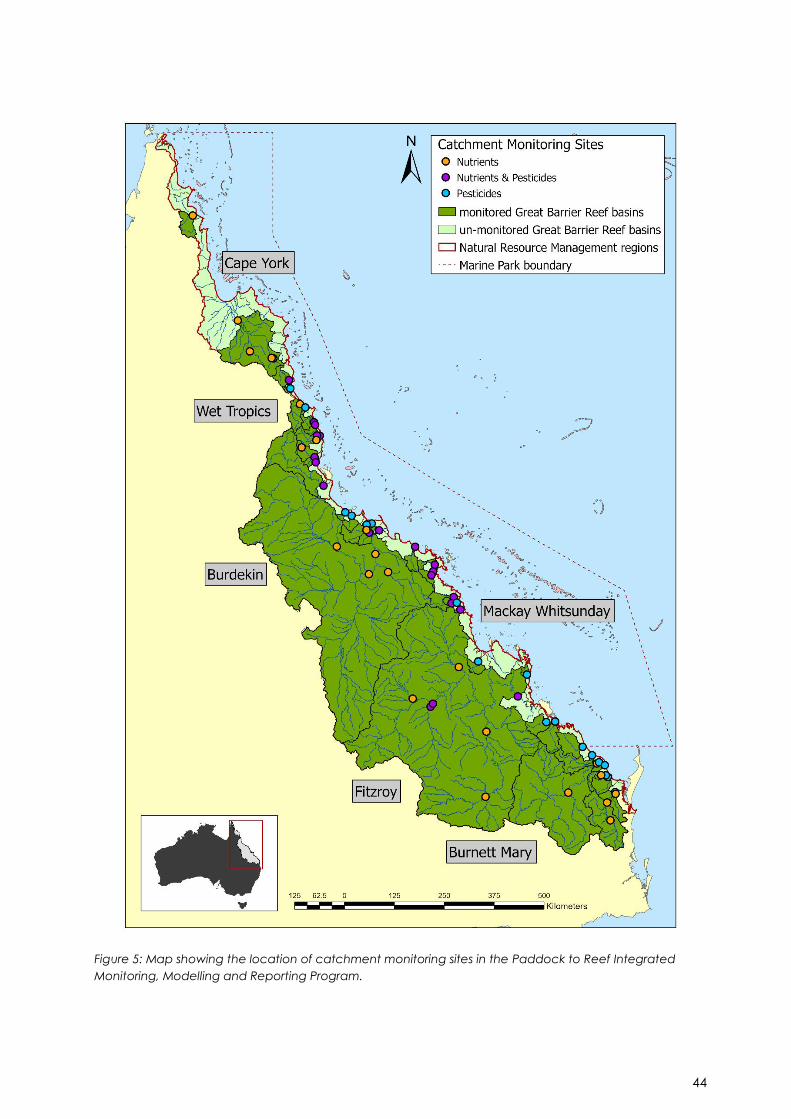
https://www.reefplan.qld.gov.au/tracking-progress/reef-report-card/methods-to-create-report-card

44

Figure 5: Map showing the location of catchment monitoring sites in the Paddock to Reef Integrated

Monitoring, Modelling and Reporting Program.

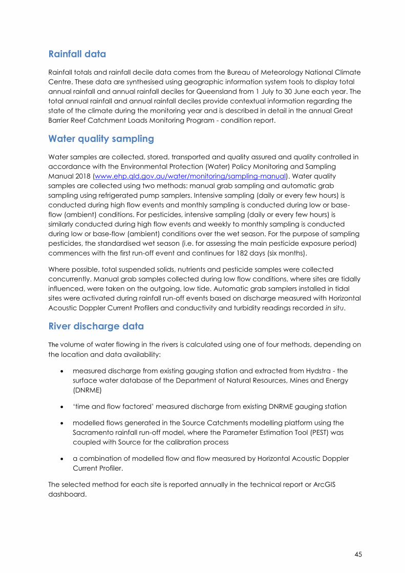
45

Rainfall data

Rainfall totals and rainfall decile data comes from the Bureau of Meteorology National Climate

Centre. These data are synthesised using geographic information system tools to display total

annual rainfall and annual rainfall deciles for Queensland from 1 July to 30 June each year. The

total annual rainfall and annual rainfall deciles provide contextual information regarding the

state of the climate during the monitoring year and is described in detail in the annual Great

Barrier Reef Catchment Loads Monitoring Program - condition report.

Water quality sampling

Water samples are collected, stored, transported and quality assured and quality controlled in

accordance with the Environmental Protection (Water) Policy Monitoring and Sampling

Manual 2018 (www.ehp.qld.gov.au/water/monitoring/sampling-manual). Water quality

samples are collected using two methods: manual grab sampling and automatic grab

sampling using refrigerated pump samplers. Intensive sampling (daily or every few hours) is

conducted during high flow events and monthly sampling is conducted during low or base-

flow (ambient) conditions. For pesticides, intensive sampling (daily or every few hours) is

similarly conducted during high flow events and weekly to monthly sampling is conducted

during low or base-flow (ambient) conditions over the wet season. For the purpose of sampling

pesticides, the standardised wet season (i.e. for assessing the main pesticide exposure period)

commences with the first run-off event and continues for 182 days (six months).

Where possible, total suspended solids, nutrients and pesticide samples were collected

concurrently. Manual grab samples collected during low flow conditions, where sites are tidally

influenced, were taken on the outgoing, low tide. Automatic grab samplers installed in tidal

sites were activated during rainfall run-off events based on discharge measured with Horizontal

Acoustic Doppler Current Profilers and conductivity and turbidity readings recorded in situ.

River discharge data

The volume of water flowing in the rivers is calculated using one of four methods, depending on

the location and data availability:

measured discharge from existing gauging station and extracted from Hydstra - the

surface water database of the Department of Natural Resources, Mines and Energy

(DNRME)

‘time and flow factored’ measured discharge from existing DNRME gauging station

modelled flows generated in the Source Catchments modelling platform using the

Sacramento rainfall run-off model, where the Parameter Estimation Tool (PEST) was

coupled with Source for the calibration process

a combination of modelled flow and flow measured by Horizontal Acoustic Doppler

Current Profiler.

The selected method for each site is reported annually in the technical report or ArcGIS

dashboard.

http://www.ehp.qld.gov.au/water/monitoring/sampling-manual

46

Water quality sample analysis

The Science Division Chemistry Centre (Dutton Park, Queensland) analyses water samples for

total suspended solids and nutrients (Table 5). The Queensland Health Forensic and Scientific

Services Organics Laboratory (Coopers Plains, Queensland) analyses water samples for

pesticides (Error! Reference source not found.). Both laboratories are accredited by the

National Association of Testing Authorities for the analyses conducted.

Table 5: Summary information for each reported analyte in the catchment monitoring program

Reported pollutants Abbreviation Measured analytes

Sediment (Total suspended solids) TSS Total suspended solids

Total nitrogen TN Total nitrogen as N

Particulate nitrogen PN Total nitrogen (suspended) as N

Dissolved organic nitrogen DON Organic nitrogen (dissolved) as N

Ammonium nitrogen as N NH4-N Ammonium nitrogen as N

Oxidised nitrogen as N NOx-N Oxidised nitrogen as N

Dissolved inorganic nitrogen DIN Ammonium nitrogen as N + Oxidised

nitrogen as N

Total phosphorus TP Total phosphorus as P

Particulate phosphorus PP Total phosphorus (suspended) as P

Dissolved organic phosphorus DOP Organic phosphorus (dissolved) as P

Dissolved inorganic phosphorus DIP Phosphate phosphorus as P

Pesticide monitoring and reporting differs from nutrients and suspended solids due to the large

range of pesticides used in agriculture and the variation in their use from one year to the next.

For this reason, water samples are analysed for a general suite of pesticides. However, not all

pesticides that are detected are reported each year. Other detected and non-detected

pesticides will be reported via the pesticide exceedance dashboard. A sub-set of pesticides,

referred to as the reference pesticides, are used to measure and model the progress towards

the pesticide target2. The reference pesticides (Error! Reference source not found.) have been

selected based on the frequency of their detection in catchments, the availability of

ecotoxicity data for individual pesticides, and their capacity to be modelled in Source

Catchment models. The reference pesticides include herbicides and insecticides used in a

range of agricultural land uses, including sugarcane, grazing, cropping and horticulture.

2 Note: The pesticide target encompasses all pesticides in GBR water bodies. All possible

measures are taken to include as many pesticides in the metric to measure progress towards the

target; however, measuring and modelling progress is reliant on other data (e.g. ecotoxicity and

application data) not just concentration information, which is not available for all pesticides

detected in catchments. For this reason, not all pesticides are included in the metric to measure

progress towards the target. The number and types of pesticides included in the metric will

expand over time as new data is collected.

47

Table 2: Pesticides included in pesticide risk metric (not all of the listed pesticides were

necessarily detected in collected water samples)

Reference

pesticide

Pesticide

type Mode of action

Chlorpyrifos Insecticide Acetylcholine esterase (AChE) inhibitor

Fipronil Insecticide Gamma-aminobutyric acid (GABA) gated chloride

channel blocker

Imidacloprid Insecticide Nicotinic receptor agonist

Haloxyfop Herbicide Acetyl-coenzyme A carboxylase (ACCase) inhibitor

Imazapic Herbicide

Acetolactate synthase (ALS) inhibitor Metsulfuron-

methyl Herbicide

Pendimethalin Herbicide Microtubule synthesis inhibitor

Metolachlor Herbicide Acetolactate synthase (ALS) inhibitor

Reference

pesticide

Pesticide

type Mode of action

Ametryn Herbicide

PSII inhibitor

Atrazine Herbicide

Terbuthylazine Herbicide

Tebuthiuron Herbicide

Simazine Herbicide

Diuron Herbicide

Terbutryn Herbicide

Hexazinone Herbicide

Metribuzin Herbicide

2,4-D Herbicide Auxin mimic (Phenoxy-carboxylic acid auxins)

MCPA Herbicide

Fluroxypyr Herbicide Auxin mimic (Pyridine-carboxylic acid auxins)

Triclopyr Herbicide

Isoxaflutole Herbicide 4-hydroxyphenylpyruvate dioxygenase (4-HPPD) inhibitor

Calculating nutrient and sediment loads

The suitability of the generated water quality monitoring data for use in load calculations was

assessed using a sample representivity rating. The annual rating of sampling representivity was

assessed against two criteria:

1. the number of samples collected in the top five per cent of annual monitored flow

2. the ratio between the highest flow rate at which a water sample was collected and

the maximum flow rate recorded.

The representivity was determined for each monitoring year by assigning a score using the

system presented in Table 3.

48

Table 6: Scores assigned to total suspended solids and nutrients data to determine their

representivity

Number of samples in top 5%

of flow

Score Ratio of highest flow sampled to

maximum flow recorded

Score

0 – 9 1 0.00 – 0.19 1

10 – 19 2 0.20 – 0.39 2

20 – 29 3 0.40 – 0.59 3

30 – 39 4 0.60 – 0.79 4

>40 5 >0.80 5

The rating of sample representivity for each analyte was the sum of the scores for the two

criteria. Sample representivity for each analyte was rated as ‘excellent’ when the total score

was greater than or equal to eight, ‘good’ when the total score was six or seven, ‘moderate’

for total scores of four or five, or ‘indicative’ when the score was less than four. Furthermore,

hydrographs were visually assessed to verify the representivity rating.

For nutrients and sediment, the concentration and flow data are used to determine the total

load of each pollutant that is transported past the monitoring site in each catchment and sub-

catchment. Annual and daily loads are calculated for total suspended solids and the nutrient

analytes listed in Error! Reference source not found. and for the catchments and sub-

catchments listed in Table 4, using the Loads Tool component of the software Water Quality

Analyser 2.1.2.6 (eWater 2012). The total suspended solids and nutrient loads were calculated

using concentrations reported in milligrams per litre (mg L-1).

One of two methods was used to calculate loads: the average load (linear interpolation of

concentration) or the Beale ratio. Average load (linear interpolation of concentration) is the

most accurate and reliable method, provided events are adequately sampled, with a

representivity rating of excellent. For complex events or events with a representivity rating of

good, moderate or indicative, the Beale ratio is one of the recommended methods (Joo et al.

2012).

Calculating the Pesticide Risk Metric

The Pesticide Risk Metric estimates the percentage of species protected (reciprocal of

percentage of species affected) from mixtures of pesticides detected during a standardised

wet season of 182 days. The wet season was determined to be the only period of time when

there was a significant risk of pesticide run-off. This metric, calculated from the monitored

concentration data for the 22 reference pesticides, was used to estimate the percentage of

species protected in each monitored catchment. It is also used to validate the Source

Catchment modelled estimates of progress, from the Pesticide Risk Baseline3, towards the

target. Note: it is intended that modelled estimates of progress towards the pesticide target will

be reported in future years.

3 The Pesticide Risk Baseline was generated using a suite of models that can predict the

pesticide mixture toxicity from monitored sites to the whole catchment, region and Great

Barrier Reef scales. The Pesticide Risk Baseline was developed using Catchment loads

monitoring program data collected from monitoring sites across Queensland from 2015 to

2018. The model build compared the monitored pesticide trends to spatial, climate and land

use characteristics at those sites. The Pesticide Risk Baseline then used the relationships

developed to predict the current estimate of percent species protected from mixtures of 22

reference pesticides observed in major catchments discharging to the Great Barrier Reef

(Warne et al. 2020).

49

In order to express the concentration data for all 22 reference pesticides as a single number

that represents the overall risk to aquatic ecosystems, the pesticide concentration data was

converted into a number that represented the toxicity of the mixture of pesticides in each

water sample. This was achieved using the multi-substance potentially affected fraction (ms-

PAF) approach (Traas et al. 2002).

The 22 reference pesticides have multiple different modes of action (Table 2). The toxicity of

pesticides with different modes of action was calculated using the independent action model

of joint action (Plackett and Hewlett 1952) within the multiple-substance-potentially affected

fraction (ms-PAF) method. Further details on how the pesticide risk metric calculations were

made are provided in Warne et al. (2020). The pesticide mixture toxicity was calculated for all

samples collected over the wet season. Where there was more than one sample per day, a

daily mean pesticide mixture toxicity value was calculated.

The mixture toxicity data (i.e. ms-PAF values) for all water samples collected over the wet

season were then summarised as a single value. This required estimating the daily average ms-

PAF for days that were not monitored during the wet season using a multiple imputation

technique (Rubin 1996; Donders et al. 2006; Patrician 2002). This involved fitting a statistical

distribution to the observed data for the wet season for the site. This distribution was then used

to impute values to fill in the missing days in the 182-day period. The resultant 182 days of data

were then divided by 182 to obtain the Pesticide Risk Metric and ranked into five risk categories

(Table 4). These categories are consistent with the ecological condition categories used in the

Australian and New Zealand Water Quality Guidelines (ANZWQG) for Fresh and Marine Waters.

The Pesticide Risk Metric method was used to obtain pesticide risk values for four groups of

pesticides - total pesticides (all 22 pesticides included in the Pesticide Risk Metric), insecticides,

photosystem inhibiting (PSII) herbicides and non-PSII herbicides.

Table 4: Risk categories used to assess pesticide risk

Pesticide Risk Metric value

Risk category Ecological condition

(ANZWQG) % species affected % species

protected

≤1% ≥99% Very low High Ecological Value

>1 to 5% 95 to <99% Low Slightly to Moderately Disturbed

>5 to 10% 90 to <95% Moderate

Highly Disturbed >10 to 20% 80 to <90% High

>20% <80% Very high

Reporting on pesticides for the report card

Pesticide monitoring data from the Great Barrier Reef Catchment Loads Monitoring Program

were used to calculate the current condition (Pesticide Risk Metric expressed as a per cent of

species protected) at each monitoring site. These data were weighted according to the size of

the sub-catchment compared to the catchment they belong to. The weighted values are

then used to modify the per cent of species protected values from the Pesticide Risk Baseline

(Warne et al. 2020), to estimate the current condition of each catchment. The same approach

was applied to the regions and the entire Great Barrier Reef Catchment Area. This method

does not enable reporting of progress to the pesticide target, as the current condition values

are affected by annual variations in climatic conditions. The relative contribution of PSII

herbicides, other herbicides and insecticides to the Pesticide Risk Metric values was also

http://www.waterquality.gov.au/anz-guidelines/resources/key-concepts/level-of-protection

50

determined for each catchment. Details of all these calculations are provided in Warne et al.

(2020).

Qualitative confidence rankings for reporting on pesticides


in the Reef water quality report card from low to high. The approach combined expert opinion

and direct measures of error for program components where available.

The methods used to calculate the Pesticide Risk Baseline for measuring progress towards the

target received a two-dot confidence ranking. The rationale for this confidence ranking is

provided below.

Rationale for the confidence ranking

Maturity of methods

A score of one was awarded because the methods have not been reviewed.

Validation

A score of two was awarded because the data used in the calculations have either been

validated or are direct measurements from monitoring (analytical results), but the per cent of

species protected have not been validated in the field nor has the method been

independently reviewed.

Representativeness

A score of one was awarded which is based on a representivity assessment for the predictions

at the whole of the Great Barrier Reef scale. This was low because the high-confidence

monitoring data at the catchment scale was used to adjust values at the catchment, region

and whole of Great Barrier Reef levels.

Directness

A score of one was awarded because the assessment used a mix of quantified assessments

(i.e. catchment monitoring data, laboratory-based ecotoxicology data); however, the per

cent of species protected at the end of catchments is not directly measured. Measured

pesticide concentrations at the catchment level are used to calculate values at the

catchment, region and whole Great Barrier Reef level.

Measurement error

A score of two was awarded because not all components have an estimate of error.

51

References

Donders, ART, Van Der Heijden, GJ, Stijnen, T, and Moons, KG 2006, ‘A gentle introduction to

imputation of missing values’, Journal of clinical epidemiology, vol. 59(10), pp. 1087-1091.

eWater Cooperative Research Centre 2012, Water Quality Analyser (Version 2.1.1.4) [computer

software], eWater Cooperative Research Centre, Canberra, Australia.

Joo, M, Raymond, MA, McNeil, VH, Huggins, R, Turner, RDR and Choy, S 2012, ‘Estimates of

sediment and nutrient loads in 10 major catchments draining to the Great Barrier Reef during

2006–2009’, Marine pollution bulletin, vol. 65 (4–9), pp. 150–166.

Patrician, PA 2002, ‘Multiple imputation for missing data’, Research in nursing and health, vol.

25(1), pp. 76-84.

Plackett, RL and Hewlett, PS 1952, ‘Quantal responses to mixtures of poisons’, Journal of the

Royal Statistical Society: Series B (Methodological), vol. 14(2), pp. 141-154.

Rubin, DB 1996, ‘Multiple imputation after 18+ years’, Journal of the American statistical

Association, vol. 91(434), pp. 473-489.

Traas, TP, van de Meent, D, Posthuma, L, Hamers, T, Kater, BJ, de Zwart, D, and Aldenberg, T

2002, ‘The potentially affected fraction as a measure of ecological risk’, In Species sensitivity

distributions in ecotoxicology, pp. 315-344.

Warne, MStJ, Neelamraju, C, Strauss, J, Smith, RA, Turner, RDR, Mann, RM 2020, Development of

a Pesticide Risk Baseline for the Reef 2050 Water Quality Improvement Plan, Department of

Environment and Science, Brisbane, Australia.

52

Marine monitoring methods

This report summarises the data and methods used for monitoring and reporting within the

Marine Monitoring Program managed by the Great Barrier Reef Marine Park Authority and

reported in the Reef Water Quality Report Card 2019 (see Figure 6 - elements other than eReefs

marine modelling). Detailed methods are available in the Marine Monitoring Program annual

technical report series that undergo independent peer review before being published in the

Great Barrier Reef Marine Park Authority’s eLibrary.

Figure 6: Main data sources, inputs and outputs for the Marine Monitoring Program, which include inshore

coral, inshore water quality and inshore seagrass monitoring. The Marine Modelling Program provides the

water quality metric based on eReefs model output.

The Marine Monitoring Program was established in 2005 and assesses trends in ecosystem

health and resilience indicators for the inshore Great Barrier Reef in relation to water quality

and its linkages to end-of-catchment pollutant loads. The inshore Marine Monitoring Program

has three sub-components:

water quality, including pesticides (Gruber et al. 2020)

seagrass condition (McKenzie et al. 2020)

coral reef condition (Thompson et al. 2020).

http://elibrary.gbrmpa.gov.au/jspui/browse?type=series&value=Marine+Monitoring+Program&sort_by=2&order=DESC&rpp=20&etal=0&submit_browse=Update

http://elibrary.gbrmpa.gov.au/jspui/browse?type=series&value=Marine+Monitoring+Program&sort_by=2&order=DESC&rpp=20&etal=0&submit_browse=Update

53

The Marine Monitoring Program is one line of evidence used to report progress towards the

Reef 2050 Water Quality Improvement Plan (Reef 2050 WQIP) (Australia and Queensland

Governments 2018) 2025 water quality outcome:

Good water quality sustains the outstanding universal value of the Great Barrier Reef,

builds resilience, improves ecosystem health, and benefits communities.

The Marine Monitoring Program objectives are:

Assess temporal and spatial trends in inshore marine water quality and link pollutant

concentrations to end-of-catchment loads.

Monitor, assess and report the condition and trend of inshore coral reefs in relation to

the extent, frequency and intensity of acute and chronic impacts.

Monitor, assess and report the condition and trend of inshore seagrass meadows in

relation to the extent, frequency and intensity of acute and chronic impacts.

Since the 2015-2016 water year, the Reef water quality report card marine result has been

based on averaging the scores for water quality from the eReefs models (Robillot et al. 2018)

with scores for coral and seagrass condition from the Marine Monitoring Program. The inshore

water quality component (see Figure 1) provides data on exposure and risk to marine

communities by analysing flood plumes and pesticide concentrations as well as in situ

measurements to detect long-term trends at specific locations and in three regions. Further

details on these methods can be found in the Marine Monitoring Program annual technical

report for inshore water quality (Gruber et al. 2020) and the annual technical report for

pesticides (Thai et al. 2020).

Seagrass condition

Monitoring is conducted in six regions, covering each major seagrass habitat type where

possible (estuarine, coastal intertidal, coastal subtidal, reef intertidal and reef subtidal) (see

Figure 7).

Sixty-nine sites at 30 locations were assessed during 2018–2019. This covered 14 coastal, four

estuarine and 12 reef locations (i.e. two or three sites at each location). Reef intertidal sites in

the Burdekin and Wet Tropics were paired with a subtidal site (McKenzie et al. 2020).

https://ereefs.org.au/ereefs

http://elibrary.gbrmpa.gov.au/jspui/browse?type=series&order=ASC&rpp=20&value=Marine+Monitoring+Program+-+Inshore+Water+Quality

http://elibrary.gbrmpa.gov.au/jspui/browse?type=series&order=ASC&rpp=20&value=Marine+Monitoring+Program+-+Inshore+Water+Quality

http://elibrary.gbrmpa.gov.au/jspui/browse?type=series&order=ASC&rpp=20&value=Marine+Monitoring+Program+-+Pesticides

http://elibrary.gbrmpa.gov.au/jspui/browse?type=series&order=ASC&rpp=20&value=Marine+Monitoring+Program+-+Pesticides

54

Figure 7: Marine Monitoring Program seagrass monitoring locations (including Queensland Parks and

Wildlife Service and Seagrass-Watch). Source: (McKenzie et al. 2020).

At each location, with the exception of subtidal sites, sampling included two sites nested within

500m of each other. Subtidal sites were not always replicated within locations. Intertidal sites

were defined as a 5.5ha area within a relatively homogenous section of a representative

seagrass community/meadow. Monitoring occurs at sites in the late dry season (September-

November) and late wet season (March/April) each year.

55

Three indicators are assessed:

seagrass abundance (per cent cover) is an assessment of the average per cent cover

of seagrass per monitoring site in relation to the Seagrass Abundance Guidelines

(McKenzie 2009)

reproductive effort is the ratio of the average number of reproductive structures

(spathes, fruits, female and male flowers) of plants on an area basis relative to the long-

term average, and provides an indication of the capacity for meadow recovery

following disturbances

tissue nutrient composition is an indicator of nutrient enrichment relative to light

available for growth (McKenzie et al. 2020).

Additional indicators of seagrass condition and resilience include species composition, relative

meadow extent and density of seeds in the seed bank (McKenzie et al. 2020).

Environmental pressures are also recorded including within-canopy water temperature, within-

canopy benthic light, sediment composition as well as macroalgae and epiphyte abundance.

Within-canopy benthic light is compared to long-term recorded light levels at individual

sites as well as daily light thresholds likely to support long-term growth requirements of

the species in these habitats (Collier et al. 2016).

Within-canopy temperature is considered in context of the number of days above

35°C. Growth reduction can occur in some species from prolonged warm water

exposure (Collier et al. 2011; Collier et al. 2016). The critical canopy temperature

threshold for photoinhibition and acute temperature stress for seagrass is 40°C

(Campbell et al. 2006).

Changes in sediment composition can be an indicator of broader environmental

changes (such as sediment and organic matter loads and risk of anoxia) and an early-

warning indicator of changing species composition.

Additional data on climate and water quality is obtained from the Bureau of Meteorology and

from the Marine Monitoring Program inshore water quality component (McKenzie et al. 2020).

Coral reef condition

Monitoring of inshore coral reef communities occurs every two years at reefs adjacent to four

regions: Wet Tropics, Burdekin, Mackay Whitsunday and Fitzroy (see Figure 3). No reefs are

included in Cape York due to logistic and occupational health and safety issues relating to

diving in coastal waters in this region. Increased monitoring of inshore coral reefs in the Burnett

Mary region is underway with results to be detailed in future report cards (Thompson et al.

2020).

Thirty-two reefs are monitored at two depths under the program, with an additional nine

inshore reefs monitored at single depths under the Australian Institute of Marine Science –

Long-Term Monitoring Program. All are included in the annual assessment of coral condition,

although not all reefs are sampled every year (Thompson et al. 2020).

56

Figure 8: Sampling locations of the Marine Monitoring Program coral monitoring. Reefs are scheduled to

be monitored biennially. Yellow indicates sites scheduled to be monitored in even years, and red dots are

scheduled to be monitored in odd years. Green dots indicate sites monitored as part of the long-term

monitoring program conducted by the Australian Institute of Marine Science. Region boundaries are

represented by coloured catchment areas. Source: (Thompson et al. 2020).

Two sites at each reef are permanently marked with fence posts at the beginning of each of

five, 20m-long, transects with smaller steel rods at the midpoint and end of each transect.

Monitoring is conducted by divers along these transects. They assess community attributes

including hard and soft coral cover, the number of hard coral juvenile colonies (up to 5cm in

diameter), proportion (per cent) of macroalgae cover, rate of change in coral cover (as an

indication of the recovery potential of the reef following a disturbance) and coral community

composition (Thompson et al. 2020).

57

Assessing status against the objectives

Improved seagrass condition

Three indicators are used to assess and report inshore seagrass condition: abundance,

reproductive effort and tissue nutrient status. Trend graphs show the combined score of the

indicators over time (colour-graded circles) as well as the indicator’s contribution to scores

(lines). Further detail about the selection and scoring of these indicators is available in the

annual technical report (McKenzie et al. 2020).

Regional scores for seagrass are derived as the unweighted averages of the three indicator

scores. Detailed information is available in the Marine Monitoring Program’s annual technical

reports published in the Great Barrier Reef Marine Park Authority’s eLibrary.

To calculate the overall score for seagrass, the regional scores were weighted on the

percentage of World Heritage Area seagrass (shallower than 15m) within that region (see Table

7).

Table 7: Area of seagrass shallower than 15m in each region within the boundaries of the Great

Barrier Reef World Heritage Area*

Region Area of seagrass

(km2)

Per cent

Cape York 2,078 0.60

Wet Tropics 207 0.06

Burdekin 587 0.17

Mackay Whitsunday 215 0.06

Fitzroy 257 0.07

Burnett Mary 120 0.03

World Heritage Area 3,464 1.00

* Derived from (McKenzie, Yoshida, Grech et al. 2014; McKenzie, Yoshida, and Unsworth 2014; Carter et al. 2016;

Waterhouse et al. 2016).

Improved coral condition

Five indicators are used to assess and report on inshore coral reef condition: coral cover, coral

cover change, juvenile coral density, coral community composition and proportional

macroalgal cover. Trend graphs show the combined score of the indicators over time (colour-

graded circles) as well as the indicator’s contribution to the scores (lines). Further detail about

the selection and scoring of these indicators is available in the annual technical report

(Thompson et al. 2020).

Regional scores for coral are derived as the unweighted averages of the five indicator scores.

Detailed information is available in the Marine Monitoring Program’s annual technical reports

published in the Great Barrier Reef Marine Park Authority’s eLibrary.

To calculate the overall score for coral, the regional scores were weighted on the percentage

of the total inshore reef area in the Great Barrier Reef Marine Park that is represented by each

of the monitored regions (see Table 8).

http://elibrary.gbrmpa.gov.au/jspui/browse?type=series&order=ASC&rpp=20&value=Marine+Monitoring+Program+-+Inshore+Seagrass

http://elibrary.gbrmpa.gov.au/jspui/browse?type=series&order=ASC&rpp=20&value=Marine+Monitoring+Program+-+Inshore+Coral+Reef+Monitoring




58

Table 8: Area of inshore reef in each region within the Marine Park*

Region Area of inshore reef

(km2)

Per cent

Cape York 264.73

Wet Tropics 64.42 0.209

Burdekin 28.23 0.092

Mackay Whitsunday 117.25 0.381

Fitzroy 97.66 0.318

Burnett Mary 4.58

Marine Park 576.85 1.00

* Area statistics supplied by the Authority’s Spatial Data Centre, 2011

Synthesis and integration of data and information

The Reef Water Quality Report Card 2019 provides scores for the condition of inshore water

quality, seagrass and coral at Great Barrier Reef-wide and regional scales.

Reef-wide and regional marine scores are unweighted averages of these three indicator

scores.

The Marine Monitoring Program provides the coral and seagrass scores, based on annual

technical reports published in the Great Barrier Reef Marine Park Authority’s eLibrary.

The eReefs Marine Modelling Program provides the water quality metric for the inshore Reef

score based on open coastal waters (Robillot et al. 2018).

Qualitative confidence rankings


in the Reef Water Quality Report Card 2019, from low to high. The approach combined expert

opinion and direct measures of error for program components where available. Seagrass and

coral both received a four-dot confidence ranking (see Figure 64).

Seagrass Coral

Figure 9: Qualitative confidence rankings for seagrass and coral scores. Source: Refer to Appendix A.



59

References

Australia and Queensland Governments. 2018. Reef 2050 Water Quality Improvement Plan

2017-2022. Brisbane: Queensland Government.

https://www.reefplan.qld.gov.au/about/assets/reef-2050-water-quality-improvement-

plan-2017-22.pdf.

Campbell, S. J., L. J. McKenzie, and S. P. Kerville. 2006. Photosynthetic Responses of Seven

Tropical Seagrasses to Elevated Seawater Temperature. Journal of Experimental Marine

Biology and Ecology 330 (2): 455-468.

Carter, A. B., S. A. McKenna, M. A. Rasheed, L. McKenzie, and R. Coles. 2016. Seagrass

Mapping Synthesis: A Resource for Coastal Management in the Great Barrier Reef World

Heritage Area: Report to the National Science Programme. Cairns: Reef and Rainforest

Research Centre Limited.

Collier, C. J., MP Adams, L. Langlois, M. Waycott, KR O’Brien, PS Maxwell, and L. McKenzie.

2016. Thresholds for Morphological Response to Light Reduction for Four Tropical Seagrass

Species. Ecological Indicators 67: 358-366.

Collier, C. J., S. Uthicke, and M. Waycott. 2011. Thermal Tolerance to Two Seagrass Species at

Contrasting Light Levels: Implications for Future Distribution in the Great Barrier Reef.

Limnology and Oceanography 56 (6): 2200-2210.

Gruber, R., J. Waterhouse, M. Logan, C. Petus, C. Howley, S. Lewis, D. Tracey, et al. 2020. Marine

Monitoring Program: Annual Report for Inshore Water Quality Monitoring 2018-2019. Report

for the Great Barrier Reef Marine Park Authority. Townsville: Great Barrier Reef Marine Park

Authority.

McKenzie, L. J., R. L. Yoshida, A. Grech, and R. Coles. 2014. Composite of Coastal Seagrass

Meadows in Queensland, Australia - November 1984 to June 2010. . PANGAEA.

http://doi.pangaea.de/10.1594/PANGAEA.826368.

McKenzie, L. J., R. L. Yoshida, and R. K. F. Unsworth. 2014. Disturbance Influences the Invasion of

a Seagrass into an Existing Meadow. Marine Pollution Bulletin 86 (1-2): 186-196.

McKenzie, L. J. 2009. Condition, Treand and Risk in Coastal Habitats: Seagrass Indicators,

Distribution and Thresholds of Potential Concern. Reef and Rainforest Research Centre,

Cairns: Marine and Tropical Research Facility. http://rrrc.org.au/wp-

content/uploads/2014/06/113-QDPIF-McKenzie-L-2009-June-Milestone-Report.pdf ;.

McKenzie, L. J., C. J. Collier, L. A. Langlois, R. L. Yoshida, J. Uusitalo, and M. Waycott. 2020.

Marine Monitoring Program: Annual Report for Inshore Seagrass Monitoring 2018-2019.

Report for the Great Barrier Reef Marine Park Authority. Townsville: Great Barrier Reef

Marine Park Authority.

Robillot, C., M. Logan, M. Baird, J. Waterhouse, K. Martin, and B. Schaffelke. 2018. Testing and

Implementation of an Improved Water Quality Index for the 2016 and 2017 Great Barrier

Reef Report Cards: Detailed Technical Report. Cairns: Report to the National

Environmental Science Programme. Reef and Rainforest Research Centre Limited.

Thai, P., C. Paxman, P. Prasad, G. Elisei, T. Reeks, G. Eaglesham, R. Yeh, D. Tracey, S. Grant, and

J. Mueller. 2020. Marine Monitoring Program: Annual Report for Inshore Pesticide

Monitoring 2018–19. Townsville: Great Barrier Reef Marine Park Authority.

https://www.reefplan.qld.gov.au/about/assets/reef-2050-water-quality-improvement-plan-2017-22.pdf

https://www.reefplan.qld.gov.au/about/assets/reef-2050-water-quality-improvement-plan-2017-22.pdf

http://doi.pangaea.de/10.1594/PANGAEA.826368

http://rrrc.org.au/wp-content/uploads/2014/06/113-QDPIF-McKenzie-L-2009-June-Milestone-Report.pdf

http://rrrc.org.au/wp-content/uploads/2014/06/113-QDPIF-McKenzie-L-2009-June-Milestone-Report.pdf

60

Thompson, A., P. Costello, J. Davidson, M. Logan, and G. Coleman. 2020. Marine Monitoring

Program: Annual Report for Inshore Coral Reef Monitoring 2017-2018. Report for the Great

Barrier Reef Marine Park Authority. Townsville: Great Barrier Reef Marine Park Authority.

Waterhouse, J., J. Brodie, C. Coppo, D. Tracey, E. da Silva, C. Howley, C. Petus, et al. 2016.

Assessment of the Relative Risk of Water Quality to Ecosystems of the Eastern Cape York

NRM Region, Great Barrier Reef. A Report to South Cape York Catchments. Townsville:

TropWATER, James Cook University.

61

Marine modelling methods

The Marine Modelling Program (Waterhouse et al. 2018) directly supports the 2050 outcome of

Reef 2050 Water Quality Improvement Plan (Reef 2050 WQIP) (Australia and Queensland

governments), which is:

“Good water quality sustains the outstanding universal value of the Great Barrier Reef, builds

resilience, improves ecosystem health and benefits communities.”

The Marine Modelling Program was established in 2016 to:

Assess trends in ecosystem health for the Great Barrier Reef in relation to water quality

and its linkages to end-of-catchment loads by predicting, assessing and reporting

trends in inshore water clarity and concentrations of chlorophyll a.

Predict physical and biogeochemical properties of Reef waters under a range of

scenarios to assess the impact of management practices and contribute to the

establishment or review of basin-level water quality targets.

Support regional and whole-of-Great Barrier Reef water quality risk assessments by

predicting the impact of rivers on the Great Barrier Reef waters under a range of

conditions.

Given the scale of the Great Barrier Reef, it would be impractical to measure and report water

quality through the entire area and at a reasonable frequency using monitoring data alone.

Satellite imaging can be used to cover this wide spatial area but is generally considered to

have lower accuracy and is seasonally affected by cloud cover. Therefore, the eReefs

modelling framework is used in conjunction with the monitored information and satellite

observations to extrapolate water quality across the entire Great Barrier Reef. The model is

used to generate the marine water quality metric.

This report describes the methods used to generate the marine water quality metric for the

period 1 October 2018 to 30 September 2019 (water year 2018-2019).

62

Marine modelling methods

Marine models which integrate physical processes and ecosystem responses play an integral

part in supporting resilience-based management and linking science and observations to

policy and decision making.

In this context, the marine component of eReefs delivers and operates numerical models

capable of simulating and predicting the physical hydrodynamic state, sediment transport,

water quality and basal ecology of the Great Barrier Reef

lagoon<https://research.csiro.au/ereefs/models/>. Together, these models provide the ability

to simulate the transport and fate of waterborne material, from the ocean or land, and assess

its impact on Reef water quality (Skerratt et al., 2019a).

In 2015-2016, as part of National Environmental Science Programme (NESP) Project 3.2.5,

eReefs models were used for the first time to report on chlorophyll a (productivity linked to

nutrient concentrations) and Secchi depth (proxy for water clarity and presence of fine

sediments) across the entire Great Barrier Reef (Robillot et al., 2018). These measures

underpinned a new water quality metric for the Reef water quality report cards. The metric

considered all six regions in calculating the Reef-wide score and is based on open coastal

waters.

The new metric is underpinned by the eReefs biogeochemical model and integrates true-

colour data from satellite images for improved accuracy in what is commonly referred to as

data assimilation (Baird et al., 2016). This integration of multiple streams of data to measure and

report on water quality differs from the previous metric which relied exclusively on model

predictions of water quality variables like chlorophyll and suspended sediments derived from

satellite data. The eReefs model has been assessed extensively against in situ observations with

detailed assessment findings available in the Technical assessment of the eReefs

biogeochemical simulation [gbr4_H2p0_B3p0_Chyd_Dcrt] against observations (Skerratt et al.,

2019b). The approach to calculating Reef water quality indices and overall scores was

independently peer-reviewed as part of NESP Project 3.2.5.

eReefs coupled hydrodynamic - biogeochemical model

The eReefs coupled hydrodynamic, sediment and biogeochemical modelling system involves

the application of a range of physical, chemical and biological process descriptions to

quantify the rate of change of physical and biological variables. The process descriptions are

generally based either on a fundamental understanding of processes or on actual

measurements when a specific process was able to be isolated and studied. The model also

requires external inputs, such as observed river flows and pollutant loads. The three

components of the model are:

The hydrodynamic 3-D model as defined by Herzfeld (2006, 2015).

The sediment transport model, which adds a multilayer sediment bed to the

hydrodynamic model grid and simulates sinking, deposition and resuspension of

multiple size classes of suspended sediment (Margvelashvili, 2009, Margvelashvili et al.,

2016).

The biogeochemical model, which simulates optical, nutrient, plankton, benthic

organisms (seagrass, macroalgae and coral), detritus, chemical and sediment

dynamics across the whole Great Barrier Reef region, spanning estuarine systems to

offshore reefs (Figure 1. Skerratt et al., 2019a).

https://research.csiro.au/ereefs/models/

https://nesptropical.edu.au/index.php/round-3-projects/project-3-2-5/

https://research.csiro.au/ereefs/wp-content/uploads/sites/34/2019/04/gbr4_H2p0_B3p0_Chyd_Dcrt_4April19.pdf

https://research.csiro.au/ereefs/wp-content/uploads/sites/34/2019/04/gbr4_H2p0_B3p0_Chyd_Dcrt_4April19.pdf

63

Figure 1: Conceptual framework of the eReefs coupled hydrodynamic-biogeochemical model. Orange

variables are optically active (i.e. either scatter or absorb light), influencing the vertical attenuation of

light and the bottom light field. The model is forced by rivers along the Reef with nutrient and sediment

loads (Baird et al., 2016) using the Source Catchments model. Source: Skerratt et al., 2019a.

Briefly, the biogeochemical model considers four groups of microalgae (small and large

phytoplankton, Trichodesmium and microphytobenthos), two zooplankton groups, four

macrophytes types (seagrass types corresponding to Zoster sp., two Halophila sp. types, and

macroalgae) and coral communities. Photosynthetic growth is determined by concentrations

of dissolved nutrients (nitrogen and phosphorus) and photosynthetically active radiation.

Overall, the model contains 23 optically active constituents (Baird et al., 2016). The

biogeochemistry model was updated in 2018 to specifically consider ultrafine sediment

particles and their impact on matters such as water clarity.

The model is currently forced with freshwater inputs from rivers along the Great Barrier Reef.

River flows for 17 rivers are obtained from the Queensland Department of Natural Resources,

Mines and Energy gauging network. Nutrient concentrations flowing in from the ocean are

obtained from the CSIRO Atlas of Regional Seas (CARS) 2009 climatology (Ridgway et al.,

2002).

River pollutant loads are obtained from the Source Catchments modelling outputs (Ellis and

Searle, 2013) up to 30 April 2019. To provide daily time series prediction of pollutant loads past

30 April,2019, pollutant generation models are used that estimate daily loads through varying

monthly concentrations. These monthly concentration outputs allow the model predictions to

be extended by providing daily rainfall run-off model inputs (i.e. the run-off of the day), without

the need to update many thousands of farm scale sub-models.

The eReefs model can be run without using observations from the marine environment, which is

referred to as a non-assimilating simulation. However, data assimilation provides the single best

estimate of the biogeochemical state of the Reef by combining modelling and observations

(Jones et al., 2016), and also improves the skill of the model to make predictions (Skerratt et al.,

2019a, b). Data assimilation systems can be thought of as using a model to interpolate

between observations.

64

For the Great Barrier Reef, only remote sensing provides the density of observations required to

undertake a large-scale data assimilation (see www.bom.gov.au/marinewaterquality). For

shallow inshore waters, using remote sensing to estimate in-water properties is challenging due

to the interactions between chlorophyll a, sediment, coloured dissolved organic matter and

benthic communities, which all absorb and scatter light in the blue and green wavebands.

Instead of using remote sensing to estimate in-water properties, the water quality metric is

based on the optical calculations of the biogeochemical model, which simulates the

normalised remote-sensing reflectance. The data assimilation system uses the mismatch

between observed and modelled remote-sensing reflectance to constrain the

biogeochemical model (Jones et al., 2016).

A 100 member Ensemble Kalman Filter (EnKF) assimilation system is used informed by observed

ocean colour from the NASA MODIS Aqua, VIIRS and ESA Sentinel-3A satellites (Jones et al.,

2016). When the ocean colour data is ingested, the model shifts a number of optically-active

in situ quantities, and in particular phytoplankton numbers, in all ensemble members in a

manner that is consistent with the statistical properties of the biogeochemical model. The

estimate of the biogeochemical state by the assimilation system is the mean of the 100

ensemble members. While the model assimilates ocean colour data from satellite, it is assessed

against the in situ observations of chlorophyll a concentration, from which the skill of the system

can be quantified.

Modelling improvements

The modelling system was initially developed under the eReefs Project and NESP 3.2.5 Project,

and improved for Report Card 2017 and 2018. Significant improvements in Report Card 2019

include:

Incorporating catchment load estimates using the new SOURCE Catchments code with

2019 vegetation cover.

Improved pre-processing of river loads before input into the model by 'capping' to

prevent large river concentrations due to large loads relative to small flows. Loads that

cannot be included at the time predicted by SOURCE Catchments are released at the

next flow event: this allows concentrations to be below the cap. This mostly affected

the O’Connell River due to large ungauged sections of the catchment.

SOURCE Catchments total suspended sediments were allocated to FineSed (90%) and

Dust (10%), replacing constant concentration for Dust of 20 g/m3 used in previous

simulations. This reduced the total riverine suspended solids slightly and increased the

fraction of ultrafine sediments during large flows.

From 1 January 2018, Sentinel-3A atmospherically-corrected remote-sensing

reflectance was used for the data assimilation.

Optical properties of suspended inorganic particles were updated based on analysis in

Soja-Wozniak et al. (2019). These new values, obtained at Lucinda Jetty Coastal

Laboratory, were more representative of the Great Barrier Reef-wide suspended

inorganic particles but less representative of coastal embayments.

The revised model has been assessed over eight years and compared to the previous model

configuration to confirm it maintained all the properties and skill required to predict water

quality.

http://www.bom.gov.au/marinewaterquality

65

How the metric is calculated and information reported

The Reef water quality report card marine water quality metric is calculated as follows:

1. Chlorophyll a concentration and Secchi depth data are extracted from the assimilated

eReefs biogeochemical model at a 4km spatial resolution and daily temporal resolution

(midday snapshot) for the entire Reef.

2. The data is partitioned temporally into water years (from 1 October to 30 September of

the reporting year) and spatially into zones representing combinations of regions and

cross-shelf water bodies (i.e. open coastal, mid-shelf and offshore waters; defined in

GBRMPA, 2010). The enclosed coastal water body is excluded due to limitations

associated with the 4 km model resolution near the coastline.

3. The site-level data (4 km x 4 km) for each of the three measures are standardised to

indices on a continuous scale of zero (very poor) to 100 (very good). This is done by

assessing individual values relative to the appropriate water quality guideline value

according to a ‘modified amplitude indexation routine’ (fsMAMP: base 2 logarithm of

the ratio of observed value to threshold).

4. Scores for each parameter are aggregated (averaged) temporally over the water year

into annual scores and spatially in the open coastal reporting zone. The resulting scores

for chlorophyll-a and Secchi depth are then averaged to generate a single score for

each region.

5. A Reef score is calculated as the weighted (relative areas) average of regional scores.

6. All reported scores are mapped onto a five-point (A–E) colour-coded grading scale

(see Table 1).

Table 9: Marine water quality metric score to grade scale

Grade Status Criteria Colour

E Very poor 0–20% Red

D Poor 21–40% Orange

C Moderate 41–60% Yellow

B Good 61–80% Light green

A Very good 81–100% Dark green



in the report card, from low to high. The approach combined expert opinion and direct

measures of error for program components where available. Marine modelling received a

three-dot confidence ranking.

66

References

Baird, ME, Cherukuru, N, Jones, E, Margvelashvili, N, Mongin, M, Oubelkheir, K, Ralph, PJ, Rizwi,

F, Robson, BJ, Schroeder, T, Skerratt, J, Steven, ADL, Wild-Allen, KA 2016, ‘Remote-sensing

reflectance and true colour produced by a coupled hydrodynamic, optical, sediment,

biogeochemical model of the Great Barrier Reef, Australia: Comparison with satellite data’,

Environmental Modelling and Software, vol. 78, pp. 79-96.

Ellis, R, Searle, R 2013, ‘An integrated water quality modelling framework for reporting on Great

Barrier Reef catchments’, in J Piantadosi, RS Anderssen and J Boland eds, MODSIM2013, 20th

International Congress on Modelling and Simulation, Modelling and Simulation Society of

Australia and New Zealand, December 2013, pp. 3183–89

<www.mssanz.org.au/modsim2013/L21/ellis.pdf>

Great Barrier Reef Marine Park Authority 2010, Water Quality Guidelines for the Great Barrier

Reef Marine Park, Great Barrier Reef Marine Park Authority, Townsville, Queensland.

Herzfeld, M 2006, ‘An alternative coordinate system for solving finite difference ocean models’,

Ocean Modelling, vol. 14 (3-4), pp. 174-196.

Herzfeld, M 2015, ‘Methods for freshwater riverine input into regional ocean models’, Ocean

Modelling, vol. 90, pp. 1–15.

Jones, E, Baird, ME, Mongin, M, Parslow, J, Skerratt, J, Lovell, J, Margvelashvili, NY, Matear, R,

Wild-Allen, KA, Robson, BJ, Rizwi, F, Oke, P, King, E, Schroeder, T, Steven, ADL and Taylor, J 2016,

‘Use of remote-sensing reflectance to constrain a data assimilating marine biogeochemical

model of the Great Barrier Reef’, Biogeosciences, vol. 13, pp. 6441–6469.

Margvelashvili, NY 2009, ‘Stretched Eulerian coordinate model for coastal sediment transport’,

Computers and Geosciences, vol. 35, pp. 1167-1176.

Margvelashvili, NY, Herzfeld, M, Rizwi, F, Mongin, M, Baird, ME, Jones, E, Schaffelke, B, King, E

and Schroeder, T 2016, ‘Emulator-assisted data assimilation in complex models’, Ocean

Dynamics, vol. 66(9), pp.1109-1124.

Ridgway, KR, Dunn, J and Wilkin, J 2002, ‘Ocean Interpolation by Four-Dimensional Weighted

Least Squares – Application to the Waters around Australasia’, Journal of Atmospheric and

Oceanic Technology, vol. 19, pp.1357-1375.

Robillot, C, Logan, M, Baird, M, Waterhouse, J, Martin, K and Schaffelke, B 2018, ‘Testing and

implementation of an improved water quality index for the 2016 and 2017 Great Barrier Reef

Report Cards’, Report to the National Environmental Science Programme, Reef and Rainforest

Research Centre Limited, Cairns, pp. 65.

Skerratt, JH, Mongin, M, Baird, ME, Wild-Allen, KA, Baird, ME, Robson, BJ, Schaffelke, B, Davies,

CH, Richardson, AJ, Margvelashvili, N, Soja-Wozniak, M, and Steven, ADL 2019a, ‘Simulated

nutrient and plankton dynamics in the Great Barrier Reef (2011-2016)’, Journal of Marine

Systems, vol. 192, pp. 51-74.

Skerratt, JH, Mongin, M, Baird, ME, Wild-Allen, KA, Robson, BJ, Schaffelke, B, Margvelashvili, N

and Soja-Wozniak, M 2019b ‘Technical assessment of the eReefs biogeochemical (BGC)

simulation [gbr4_H2p0_B3p0_Chyd_Dcrt] against observations’ CSIRO, Hobart, 165pp.

<https://research.csiro.au/ereefs/models/model-

outputs/bgcv3p0/gbr4_h2p0_b3p0_chyd_dcrt_4april19/>

Soja-Wozniak, M., M. Baird, T. Schroeder, Y. Qin, L. Clementson, B. Baker, D. Boadle, V. Brando,

A. Steven (2019). Particulate backscattering ratio as an indicator of changing particle

composition in coastal waters: Observations from Great Barrier Reef waters. Journal of

Geophysical Research: Oceans, 124. https://doi.org/10.1029/2019JC014998.

https://research.csiro.au/ereefs/models/model-outputs/bgcv3p0/gbr4_h2p0_b3p0_chyd_dcrt_4april19/

https://research.csiro.au/ereefs/models/model-outputs/bgcv3p0/gbr4_h2p0_b3p0_chyd_dcrt_4april19/

https://doi.org/10.1029/2019JC014998

67

Waterhouse, J, Lønborg, C, Logan, M, Petus, C, Tracey, D, Lewis, S, Howley, C, Harper, E, Tonin,

H, Skuza, M, Doyle, J, Costello, P, Davidson, J, Gunn, K, Wright, M, Zagorskis, I, Kroon, F, Gruber,

R 2018, ‘Marine Monitoring Program: Annual report for inshore water quality monitoring 2016-

2017’, Australian Institute of Marine Science, TropWATER.

Reef Water Quality Report Card 2019 Methods

Documents

Transcript of Reef Water Quality Report Card 2019 Methods