Reductions of Young tableau bijections

Igor Pak

Massachusetts Institute of TechnologyCambridge, MA 02138 USAe-mail: pak@math.mit.edu

and

Ernesto Vallejo

Instituto de Matematicas, Unidad Morelia, UNAMApartado Postal 61-3, Xangari58089 Morelia, Mich., MEXICO

e-mail: vallejo@matmor.unam.mx

June 23, 2004

Abstract

We introduce notions of linear reduction and linear equivalence of bijectionsfor the purposes of study bijections between Young tableaux. Originating inTheoretical Computer Science, these notions allow us to give a unified view of anumber of classical bijections, and establish formal connections between them.

Introduction

Combinatorics of Young tableaux is a beautiful subject which originated in the worksof Alfred Young over a century ago, and has been under intense development in thepast decades because of its numerous applications [12, 28, 36, 43]. The amazing growthof the literature and a variety of advanced extensions and generalizations led to someconfusion even about the classical combinatorial results in the subject. It seems thatuntil now, researchers in the field have not been able to unify the notation, techniques,and systematize their accomplishments.

In this paper we concentrate on bijections between Young tableaux, a classicaland the most a combinatorially effective part of subject. The notable bijections in-clude Robinson-Schensted-Knuth correspondence, Jeu de Taquin, Schutzenberger in-volution, Littlewood-Robinson map, and Benkart-Sottile-Stroomer’s tableau switching.

1

The available descriptions of these bijections are so different, that a casual reader re-ceives the impression that all these maps are only vaguely related to each other. Eventhough there is a number of well-known and important connections between some ofthese bijections, these results are sporadic and until this work did not fit any generaltheory. The idea of this paper is to give a formal general approach to positively resolvethis problem, and place these bijections under one roof, so to speak.

We introduce new notions of linear reduction and linear equivalence of bijections,and show that the above mentioned bijections are linearly equivalent. This gives thefirst rigorous result showing that these bijections are “all the same” in a certain precisesense. A benefit of this approach is that we obtain a number of new properties ofYoung tableau bijections, establish several unexpected connections between them, andeven discover a few “traditional style” conjectures. We elaborate here on the natureand the origin of our approach, while leaving definitions and main results to the nexttwo sections.

The philosophy behind this paper is the basic idea that Young tableau bijectionsare significantly different from almost all classical bijections in combinatorics, andthat a complexity approach captures this difference. On the one hand, the universe ofcombinatorial bijections is quite heterogenous: some bijections are canonical while someare inherently non-symmetric, some are recursive while some are direct and explicit,some are very natural and easy to find while some are highly nontrivial and theirdiscovery is a testament to human ingenuity (see e.g. [30, 43]). On the other hand,there is a property that almost all of them share and this is that they can be computedin the linear number of steps (see below). This is what explains why proofs of theirvalidity tend to be relatively straightforward, even if bijections’ construction may seemcomplicated. Similarly, the way bijections transfer combinatorial statistics betweensets, tend to be relatively transparent, which accounts for effectiveness of such bijectionsin the majority of successful applications.

In contrast, Young tableau bijections are substantially harder to establish, theirworking is delicate and proving their properties is subtle (as is witnessed by the valid-ity of the Jeu de Taquin, the duality of the RSK correspondence, and the many decadesthat passed before the Littlewood-Robinson correspondence was formally proved). Toexplain this phenomenon we make two observations. First, we observe that all thesebijections are inherently nonlinear and require∗ roughly O(N 3/2) number of arithmeticand logical operations (in the size N it takes to encode the tableaux). Second, weshow that any of these bijections can be used to construct any other. This explainsthe identical power 3/2 in all cases, and at the same time asserts that all these “ex-ceptionally hard” bijections are “essentially the same” and thus form a single class of“counterexamples to the rule” (that all bijections can be computed in linear time).Making these claims rigorous is a difficult task which required the introduction of new

∗We do not prove the lower bound, only the upper bound on the time complexity.

2

notation, definitions, and tools.Following ideas of Theoretical Computer Science, we view each bijection as an

algorithm with one type of combinatorial objects as the input, and another as anoutput. To make a distinction, we say that a correspondence is a one-to-one mapestablished (produced) by a bijection. Thus, several different bijections can define

the same correspondence (cf. [30]). The complexity, or the cost of the algorithm, is,roughly, the number of steps in the bijection. One can think of a correspondence asa function which is computed by the algorithm (a bijection). In contrast with theemphasis in Cryptography, our correspondences (and their inverses!) are relativelyeasy to compute. On the contrary, the bijections we analyze play an important role inAlgebraic Combinatorics in part due to this fact.

Now, as it is the case in Computational Complexity, finding lower bounds for thecost of bijections defining a given correspondence is a hard problem; we do not approachthis question in the paper. Instead, we utilize what is known as Relative Complexity, anapproach based on reduction of combinatorial problems. The reader may recall thatthe class of NP-complete problems is closed under polynomial time reductions [14].Similar notions exist for a variety of problems in low complexity classes, with variousrestrictions on time and space of the algorithms (see e.g. [33]).

In this paper we consider only linear time reductions; since the bijections weconsider require subquadratic time the reductions have to preserve that. Formally, wesay that function f reduces linearly to g, if one can compute f in time linear in thetime it takes to compute g. We say that f and g are linearly equivalent if f reduceslinearly to g and vice versa. This defines an equivalence relation on functions; it nowcan be translated into a linear equivalence on combinatorial bijections.

Our main result is a linear equivalence of the Young tableau bijections mentionedabove, as well as few other known and new bijections. To present a (skew, semistan-dard) Young tableau with ≤ k (possibly empty) rows and entries ≤ k, we need to write(

k+12

)integers ai,j which represent the number of j’s in i-th row. Ignoring the size

of ai,j, this gives input of size O(k2). Now, we shall see that all the bijections describedabove use the same subquadratic number O(k3) of arithmetic and logical operations†.This is in sharp contrast with the Young tableau bijections of linear cost, defined in theprevious paper by the authors [32]. Roughly, we showed there that O(k2) is the cost ofbijections between several combinatorial interpretations of the Littlewood-Richardson’scoefficients. This comes from the fact that bijections in [32] are given by simple lineartransformations, while Young tableau maps in this paper are inherently nonlinear.

Despite our exhaustive search through the literature, it seems that ComputationalComplexity has never been used in this area of Algebraic Combinatorics. In fact,we were able to find very few references with any kind of computational approach(see [4, 44] for rare examples). Of course, this is in sharp contrast with other parts of

†Taking N = k2 this gives O(N3/2) time mentioned above.

3

Combinatorics such as Graph Theory, Discrete Geometry, or Probabilistic Combina-torics, where computational ideas led to important advances and shift in philosophy.We hope this paper will serve a starting point in the future investigations of complexityof combinatorial bijections.

We now elaborate on the content and the structure of the paper. As the reader willsee, this paper is far from being self-contained. In fact, we never even define some ofthe classical Young tableau bijections and in most proofs we assume that the readeris familiar with the subject. This decision was largely forced upon us, to keep thepaper of manageable size. On the other hand, we are careful to include a numberof propositions giving properties and often alternative definitions of these bijections.Thus, much of the paper (the nontechnical part) can be read by the reader unfamiliarwith the subject, although in this case some of our results may seem unmotivated,inelegant, or even simplistic.

The structure of the paper is unusual as we try to emphasize the results themselvesrather than the technical details in the proofs. We start by giving basic definitions andlisting the classical maps, in terms of combinatorial objects they act upon (section 1).Even the reader well familiar with the subject is encouraged to quickly go through theseto become familiar with our notation. We then present our new framework (of linearreductions) and immediately state main results (Section 2). In Section 3 we presentproperties of the bijections, connecting them to each other through known results inthe literature. Section 4 consists of a number of small subsections which give linearreductions between various pairs of these bijections. This section represents the mainpart of the proof; proofs of technical lemmas and other details are given in Section 5.In Section 6 we describe several conjectures and other important bijections worthy ofanalysis. Final remarks are given in Section 7.

We should mention that throughout the first four sections we make no references tothe literature. Instead, in Subsection 5.1 we present a very brief overview of the liter-ature together with citation of sources containing the propositions. Further referencesare given in Section 6.

Notation. We denote partitions by Greek letters: λ, µ, ν, π, σ, τ, . . . while mapsare denoted by different Greek letters: ϕ, ψ, φ, ζ, ξ, ρ, η, . . . Young tableaux are denotedby A,B,C, . . . generic sets of partitions are denoted by A,B, C, . . . and integer arrays(weights of the tableaux) are denoted by a,b,m, . . . All Young diagrams and Youngtableaux are presented in English notation [12, 43]. Finally, we use N = 1, 2, . . . andZ≥0 = 0, 1, 2, . . ..

We should alert the reader to the fact that we use “Proposition” mainly to describeknown results, and we reserve “Theorem” and “Lemma” for the new results.

4

1 Basic definitions

1.1 Young diagrams and Young tableaux

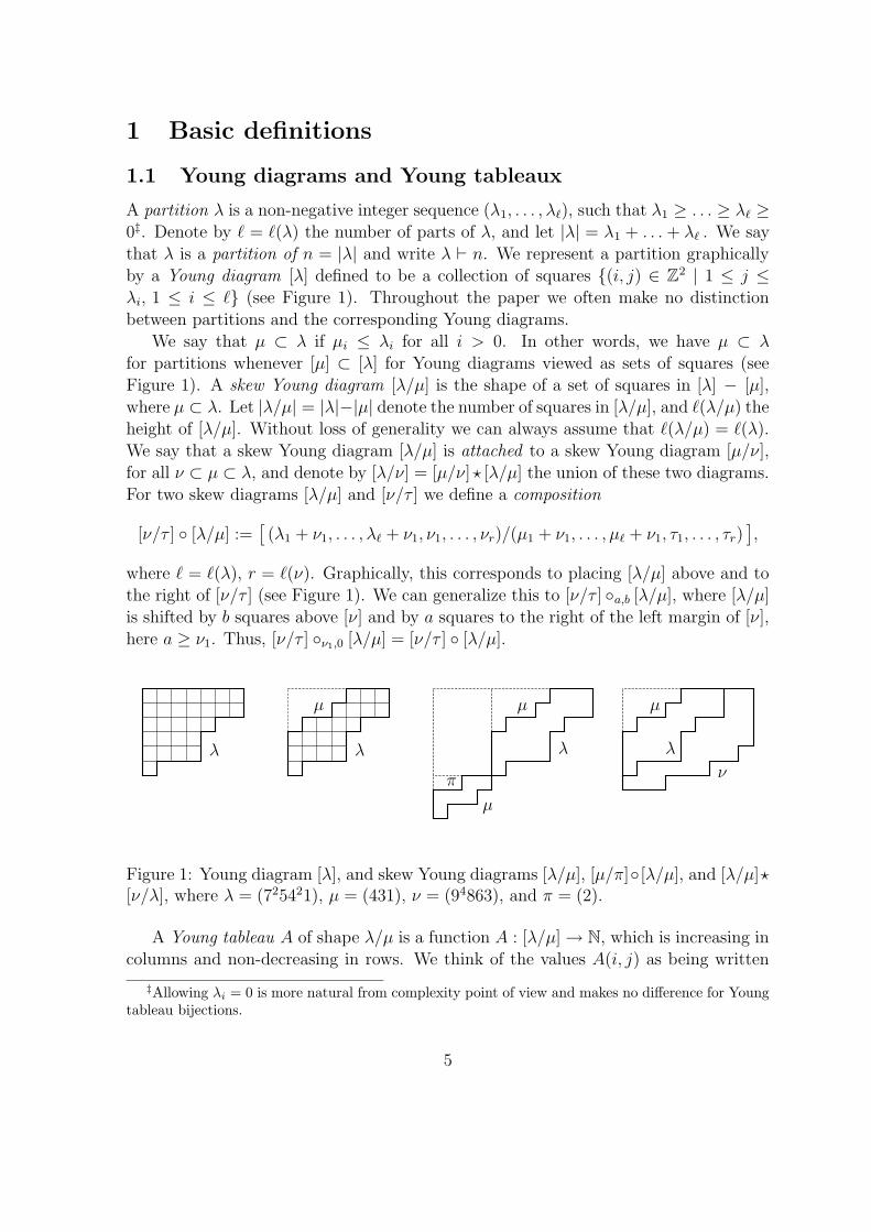
A partition λ is a non-negative integer sequence (λ1, . . . , λ`), such that λ1 ≥ . . . ≥ λ` ≥0‡. Denote by ` = `(λ) the number of parts of λ, and let |λ| = λ1 + . . . + λ` . We saythat λ is a partition of n = |λ| and write λ ` n. We represent a partition graphicallyby a Young diagram [λ] defined to be a collection of squares (i, j) ∈ Z2 | 1 ≤ j ≤

λi, 1 ≤ i ≤ ` (see Figure 1). Throughout the paper we often make no distinctionbetween partitions and the corresponding Young diagrams.

We say that µ ⊂ λ if µi ≤ λi for all i > 0. In other words, we have µ ⊂ λ

for partitions whenever [µ] ⊂ [λ] for Young diagrams viewed as sets of squares (seeFigure 1). A skew Young diagram [λ/µ] is the shape of a set of squares in [λ] − [µ],where µ ⊂ λ. Let |λ/µ| = |λ|−|µ| denote the number of squares in [λ/µ], and `(λ/µ) theheight of [λ/µ]. Without loss of generality we can always assume that `(λ/µ) = `(λ).We say that a skew Young diagram [λ/µ] is attached to a skew Young diagram [µ/ν],for all ν ⊂ µ ⊂ λ, and denote by [λ/ν] = [µ/ν]? [λ/µ] the union of these two diagrams.For two skew diagrams [λ/µ] and [ν/τ ] we define a composition

[ν/τ ] [λ/µ] :=[(λ1 + ν1, . . . , λ` + ν1, ν1, . . . , νr)/(µ1 + ν1, . . . , µ` + ν1, τ1, . . . , τr)

],

where ` = `(λ), r = `(ν). Graphically, this corresponds to placing [λ/µ] above and tothe right of [ν/τ ] (see Figure 1). We can generalize this to [ν/τ ] a,b [λ/µ], where [λ/µ]is shifted by b squares above [ν] and by a squares to the right of the left margin of [ν],here a ≥ ν1. Thus, [ν/τ ] ν1,0 [λ/µ] = [ν/τ ] [λ/µ].

PSfrag replacementsλλλλ

µ

µ

µµ

νπ

Figure 1: Young diagram [λ], and skew Young diagrams [λ/µ], [µ/π] [λ/µ], and [λ/µ]?[ν/λ], where λ = (725421), µ = (431), ν = (94863), and π = (2).

A Young tableau A of shape λ/µ is a function A : [λ/µ] → N, which is increasing incolumns and non-decreasing in rows. We think of the values A(i, j) as being written

‡Allowing λi = 0 is more natural from complexity point of view and makes no difference for Youngtableau bijections.

5

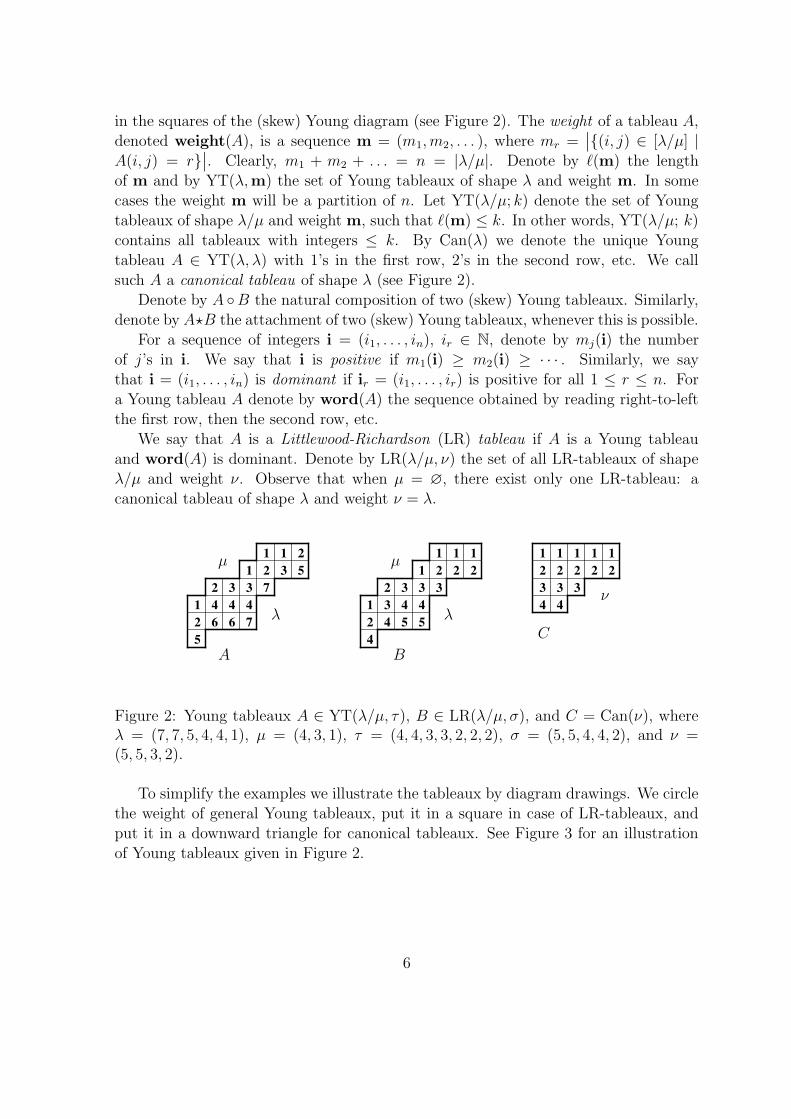
in the squares of the (skew) Young diagram (see Figure 2). The weight of a tableau A,denoted weight(A), is a sequence m = (m1,m2, . . . ), where mr =

∣∣(i, j) ∈ [λ/µ] |A(i, j) = r

∣∣. Clearly, m1 + m2 + . . . = n = |λ/µ|. Denote by `(m) the lengthof m and by YT(λ,m) the set of Young tableaux of shape λ and weight m. In somecases the weight m will be a partition of n. Let YT(λ/µ; k) denote the set of Youngtableaux of shape λ/µ and weight m, such that `(m) ≤ k. In other words, YT(λ/µ; k)contains all tableaux with integers ≤ k. By Can(λ) we denote the unique Youngtableau A ∈ YT(λ, λ) with 1’s in the first row, 2’s in the second row, etc. We callsuch A a canonical tableau of shape λ (see Figure 2).

Denote by A B the natural composition of two (skew) Young tableaux. Similarly,denote by A?B the attachment of two (skew) Young tableaux, whenever this is possible.

For a sequence of integers i = (i1, . . . , in), ir ∈ N, denote by mj(i) the numberof j’s in i. We say that i is positive if m1(i) ≥ m2(i) ≥ · · · . Similarly, we saythat i = (i1, . . . , in) is dominant if ir = (i1, . . . , ir) is positive for all 1 ≤ r ≤ n. Fora Young tableau A denote by word(A) the sequence obtained by reading right-to-leftthe first row, then the second row, etc.

We say that A is a Littlewood-Richardson (LR) tableau if A is a Young tableauand word(A) is dominant. Denote by LR(λ/µ, ν) the set of all LR-tableaux of shapeλ/µ and weight ν. Observe that when µ = ∅, there exist only one LR-tableau: acanonical tableau of shape λ and weight ν = λ.

1 2152 31

733244417662

5

1 1122 21

333244315542

4

12

1 12

3

1

332 2

44

12

PSfrag replacements

A B

Cλ λ

µµ

ν

Figure 2: Young tableaux A ∈ YT(λ/µ, τ), B ∈ LR(λ/µ, σ), and C = Can(ν), whereλ = (7, 7, 5, 4, 4, 1), µ = (4, 3, 1), τ = (4, 4, 3, 3, 2, 2, 2), σ = (5, 5, 4, 4, 2), and ν =(5, 5, 3, 2).

To simplify the examples we illustrate the tableaux by diagram drawings. We circlethe weight of general Young tableaux, put it in a square in case of LR-tableaux, andput it in a downward triangle for canonical tableaux. See Figure 3 for an illustrationof Young tableaux given in Figure 2.

6

PSfrag replacements

A BC

λλ

µµ

ν

νστ

Figure 3: Illustrations of Young tableaux A ∈ YT(λ/µ, τ), B ∈ LR(λ/µ, σ), andC = Can(ν).

1.2 Main bijections

Here we present only the notation and set-theoretic statements of the bijections. Thesebijections will be further studied in Section 3.

Let a = (a1, . . . , ak), b = (b1, . . . , bk), such that ai, bj ∈ Z≥0 and |a| = |b|, i.e.a1 + · · · + ak = b1 + · · · + bk = N . Denote by Mat(a,b) the set of k × k matricesV = (vi,j), such that vi,j ∈ Z≥0 and

k∑

j=1

vi,j = ai ,

k∑

i=1

vi,j = bj , for all 1 ≤ i, j ≤ k .

1) The Robinson-Schensted-Knuth (RSK) correspondence is a one-to-one corre-spondence

ϕ : Mat(a,b) −→⋃

λ`N

YT(λ,b) × YT(λ, a),

where |a| = |b| = N as above. Recall that if ϕ(V ) = (B,A), then B is called theinsertion tableau and A is called the recording tableau, that is, B is the P -tableau andA is the Q-tableau.

2) Let µ ⊂ λ and a = (a1, . . . , am) be a sequence of non-negative integers suchthat n = |a| = |λ/µ|. Jeu de Taquin is a map

ψ : YT(λ/µ, a) −→⋃

π`n

YT(π, a).

We should emphasize that ψ is neither an into nor an onto map. As we shall see later,it plays a central role in the universe of Young tableau bijections.

3) In notation of the Jeu de Taquin map, the Littlewood-Robinson map is givenby the following one-to-one correspondence:

φ : YT(λ/µ, a) −→⋃

π`n

YT(π, a) × LR(λ/µ, π).

7

4) Suppose now that µ ⊂ λ and c, d are sequences of non-negative integers suchthat n = |λ/µ| = |c| + |d|. Tableau Switching is a one-to-one correspondence:

ζ :⋃

π `|λ|−|c|

YT(π/µ,d) × YT(λ/π, c) −→⋃

σ `|λ|−|d|

YT(σ/µ, c) × YT(λ/σ,d).

4′) We shall need a special notation for Tableau Switching in case µ is the emptypartition, that is for normal shapes:

ζN :⋃

π `|d|

YT(π,d) × YT(λ/π, c) −→⋃

σ `|c|

YT(σ, c) × YT(λ/σ,d).

5) Let a = (a1, . . . , am) be an integer sequence, such that |a| = |λ/µ|. Considera sequence a∗ := (am, . . . , a1). Clearly, |a∗| = |λ/µ| as well. The Schutzenberger

involution is a one-to-one correspondence:

ξ : YT(λ/µ, a) → YT(λ/µ, a∗).

5′) We shall also need a special notation for the Schutzenberger involution fornormal shapes:

ξN : YT(λ, a) → YT(λ, a∗).

6) There is a different one-to-one correspondence of the same kind as ξ calledreversal:

χ : YT(λ/µ, a) → YT(λ/µ, a∗).

This correspondence has certain advantages over the Schutzenberger involution, andwill be useful for the proofs.

7), 8) Finally, suppose ν ` |λ/µ|. The Fundamental Symmetry is a one-to-onecorrespondence:

ρ : LR(λ/µ, ν) → LR(λ/ν, µ).

In this paper we define several versions of the Fundamental Symmetry map, and themain results cover the First and the Second Fundamental Symmetry maps. In gen-eral, we say that a map gives the Fundamental Symmetry map if it is a one-to-onecorrespondence between sets as above.

1.3 Computational preliminaries

Let D = (d1, . . . , dn) be an array of integers, and let m = m(D) := maxi di. The bit-size of D, denoted by 〈D〉, is the amount of space required to store D. For simplicityeverywhere below we assume that 〈D〉 = n dlog2m+ 1e.

8

We view a bijection τ : A → B as an algorithm which inputs A ∈ A and out-puts B = τ(A) ∈ B. We need to present Young tableaux as arrays of integers so thatwe can store them and compute their bit-size.

Suppose A ∈ YT(λ/µ; k). An important way to encode A is through a matrix,often called the Gelfand-Tsetlin (GT) pattern (ai,j) of the tableau, whose entries satisfycertain inequalities which are irrelevant for the purposes of this paper. It is defined byai,0 = µi and ai,j = µi + the number of integers in row i which are ≤ j, for 1 ≤ i ≤

`(λ/µ) and 1 ≤ j ≤ k. The tableau A can be now be viewed as a matrix (ai,j); this isthe way Young tableaux will be presented in the input and output of the algorithms.Another useful way to encode A is through its recording matrix (ci,j), which is definedby ci,j = ai,j − ai,j−1; in other words, ci,j is the number of j’s in the i-th row of A.

Finally, we say that a map γ : A → B is size-neutral if the ratio 〈γ(A)〉/〈A〉 isbounded for all A ∈ A. Throughout the paper we consider only size-neutral maps,often without emphasizing it. See the remark following Theorem 2 (Section 2.2) on thereasoning behind this definition.

2 Reductions of bijections and main results

2.1 Linear reductions

Think of a bijection, or any explicit map in general, as an algorithm with input andoutput written as an array of integers. Hereafter by size of the input/output we meanbit-size. As before, let 〈A〉 denote the bit-size of the integer array A. We also say thata bijection or an explicit map defines a correspondence between input and output set.Clearly, many different bijections can define the same one-to-one correspondence.

Let A and B be two possibly infinite sets of finite integer arrays, and let δ : A → B

be an explicit map between them. We say that δ has linear cost if δ computes δ(A) ∈ Bin linear time O(〈A〉) for all A ∈ A.

There are many ways to construct new bijections out of existing ones. We call suchalgorithms circuits and define below several of them that we need.

1) Suppose δ1 : A → X1, γ : X1 → X2 and δ2 : X2 → B, such that δ1 and δ2 havelinear cost. Consider χ = δ2 γ δ1 : A → B. We call this circuit trivial and denote itby I(δ1, γ, δ2).

2) Suppose γ1 : A → X , γ2 : X → B, and let χ = γ2 γ1 : A → B. We call thiscircuit sequential and denote it by S(γ1, γ2).

3) Suppose δ1 : A → X1 × X2, γ1 : X1 → Y1, γ2 : X2 → Y2, and δ2 : Y1 × Y2 → B,such that that δ1 and δ2 have linear cost. Consider χ = δ2 (γ1 × γ2) δ1 : A → B. Wecall this circuit parallel and denote it by P (δ1, γ1, γ2, δ2).

Fix a bijection β. We say that ג is a β-based ps-circuit if one of the following holds:

9

• ג = δ, where δ has linear cost.• ג = I(δ1, β, δ2).• ג = P (δ1, γ1, γ2, δ2), where γ1, γ2 are β-based ps-circuits.• ג = S(γ1, γ2), where γ1, γ2 are β-based ps-circuits.

In other words, ג is a β-based ps-circuit if there is a parallel-sequential algorithm whichuses only a finite number of linear cost maps and a finite number of maps β. The β-costof ג is the number of times the map β is used; we denote it by s(ג).

Let γ : A → B be a map produced by the β-based ps-circuit .ג We say that ג

computes γ at cost s(ג) of β.

We say that a map α is linearly reducible to β, write α → β, if there exist a finiteβ-based ps-circuit ג which computes α. In this case we say that α can be computed inat most s(ג) cost of β.

We say that maps α and β are linearly equivalent, write α ∼ β, if α is linearlyreducible to β, and β is linearly reducible to α.

2.2 Main results

Our first result is the linear equivalence of Young tableau bijections given in Section 1.2.

Theorem 1. The following maps are linearly equivalent:

1) RSK map ϕ.

2) Jeu de Taquin map ψ.3) Littlewood-Robinson map φ.

4) Tableau Switching map ζ.5) Schutzenberger involution for normal shapes ξN.

6) Reversal χ.7) First Fundamental Symmetry map ρ1.8) Second Fundamental Symmetry map ρ2.

Moreover, each of these maps can be computed in at most 36 times the cost of anyother map.

The following theorem gives a positive result about the efficient computation ofmaps 1) − 8).

Theorem 2. For the eight maps 1) − 8) as in Theorem 1, let k and m be defined asfollows:

1) k := max`(a), `(b), m := max∑

i ai,∑

j bj,

2) , 3) , 5) , 6) k := `(a), m := λ1,4) k := max`(c), `(d), m := λ1,7) , 8) k := `(ν), m := λ1.

Then the image of maps 1) − 8) can be computed at a cost of O(k3 logm).

10

We should emphasize that the standard definitions of these maps give a weakerresult. For example, Jeu de Taquin as defined in the literature (see e.g. [36, 43])requires O(|µ| · |λ/µ|) square moves, much greater than the bound above.

Remark 1. It may seem that by Theorem 1, it suffices to establish the efficientcomputation of any one of the maps. This is not the case since we compare the mapsby the number of times other maps are used, not by the timing. A priori it can(and does) happen that the maps increase the bit-size of combinatorial objects, whenthey transform the input into the output. This affects the timing of the subsequentapplications of these maps. To control this, we show that all maps we consider arein fact size-neutral, so Theorem 1 remains applicable in this case. We formalize thisobservation in Section 5.4; for now we suggest the reader simply views linear reductionsas if they were reductions on the time complexity of the maps.

3 Properties of bijections

3.1 Bender-Knuth transformations

Define Bender-Knuth (BK) transformations s1, s2, . . . as follows. Consider a Youngtableau A ∈ YT(λ/µ, a). Let m = `(a) be the length of a, and let (ai, j) be thecorresponding GT-pattern. For any 1 ≤ r < m, let B = sr(A) be a Young tableausuch that the corresponding GT-pattern (bi, j) is defined as follows:

bi, j =

minai,r+1, ai−1,r−1 + maxai,r−1, ai+1,r+1 − ai,r , if j = r,

ai,j , otherwise.

Observe that BK-transformations are defined by bijections

si : YT(λ/µ, a) → YT(λ/µ, a′), si : A 7→ B,

where a = (a1, . . . , ai, ai+1, . . . , am), and a′ = (a1, . . . , ai+1, ai, . . . , am). They alsosatisfy the following relations:

(♦) s2i = 1 , sisj = sjsi , if |i− j| ≥ 2 .

Now define elements tr, m−r and zm as follows:

zm = (s1)(s2s1)(s3s2s1) · · · (sm−1 · · · s2s1),

tr, m−r = (sm−rsm−r+1 · · · sm−1) · · · (s2s3 · · · sr+1)(s1s2 · · · sr),

where 1 ≤ r < m. By definition,

zm : YT(λ/µ, a) → YT(λ/µ, a∗), tr, m−r : YT(λ/µ, a) → YT(λ/µ,b),

11

where a∗ = (am, . . . , ar+1, ar, . . . , a1), and b = (ar+1, . . . , am, a1 . . . , ar). The mapssatisfy the following well-known relations:

(z) z2m = 1, tr, m−r tm−r, r = 1.

We shall also need the following relation:

(~) zl+k = zk tl, k zl .

It will be proved in Section 5.2.

Proposition 1. The Schutzenberger involution map ξ coincides with the map zm

defined as above: ξ = zm.

Let µ ⊂ π ⊂ λ be partitions and c, d be vectors of non-negative integers suchthat |λ/µ| = |c| + |d|. Denote r = `(d) and m = `(c) + `(d). Let A ∈ YT(λ/π, c),B ∈ YT(π/µ,d). Let A denote the tableau obtained from A by adding r to each entryof A. Denote e = (c1, . . . , cm−r, d1, . . . , dr) and f = (d1, . . . , dr, c1, . . . , cm−r). ConsiderB ? A ∈ YT(λ/µ, f); thus, tr,m−r(B ? A) ∈ YT(λ/µ, e). Decompose this tableau as

A′ ? B with A′ ∈ YT(σ/µ, c), for some partition σ of |µ| + |c|, and B ∈ YT(λ/σ).Let B′ be obtained from B by subtracting m − r to each one of its entries, so thatB′ ∈ YT(λ/σ,d). Finally, let tr,m−r(B,A) = (A′, B′).

Proposition 2. The Tableau Switching map ζ coincides with the map tr,m−r definedas above.

3.2 Jeu de Taquin is everywhere

Consider the RSK map first. Let ϕ : V 7→ (B,A), where V = (vi,j) ∈ Mat(a,b), and`(a) = `(b) = k. Define [π/σ] = [a1] [a2] · · · [ak] and [ρ/τ ] = [b1] [b2] · · · [bk].

Proposition 3. Let Y be the Young tableau in Y T (π/σ,b) that has exactly vi,j entriesequal to j in row (k+ 1)− i. Then, for the Jeu de Taquin map ψ, one has ψ(Y ) = B.

Similarly, if X is the Young tableau in Y T (ρ/τ, a) that has exactly vj,i entries equal toj in row (k + 1) − i. Then ψ(X) = A.

Let A ∈ YT(λ/π, a), B ∈ YT(π,b). Denote by (A′, B′) = ζN(B,A) their tableauswitching, where A′ ∈ YT(σ, a), B ′ ∈ YT(λ/σ,b) for some σ ` |λ/π|.

Proposition 4. In the notation above, the image (A′, B′) of (B,A) under the TableauSwitching map ζ satisfies A′ = ψ(A).

One can obtain the Jeu de Taquin map ψ as a projection of the Littlewood-Robinsonmap φ onto the first component.

12

Proposition 5. Let the image of the Littlewood-Robinson map φ(A) = (B,C). Thenψ(A) = B.

Let [λ] be Young diagram, and let [r`] be the smallest size rectangle containing [λ],i.e. ` = `(λ) and r = λ1. Denote by [λ•] a skew Young diagram [r`/(r−λ`, . . . , r−λ1)].If A ∈ YT(λ, a) is a Young tableau corresponding to a recording matrix C = (ci, j), letA• ∈ YT(λ•, a∗) by a tableau corresponding to a recording matrix C• = (c`+1−i, k+1−j).

Proposition 6. The image of the Schutzenberger involution map ξN(A) coincides with

the image ψ(A•).

Note that Propositions 4 and 6 do not have natural extensions to skew Youngdiagrams.

3.3 Hidden symmetries of RSK

The first hidden symmetry is called duality and has already been used in Proposition 3.

Proposition 7. Suppose ϕ(V ) = (B,A). Then ϕ(V ′) = (A,B), where V ′ is thetranspose matrix of V .

The second symmetry is as classical as duality but not as well-known. For anyV = (vi,j) ∈ Mat(a,b) of size k × k we denote V ∗ := (vk+1−i, k+1−j) ∈ Mat(a∗,b∗).

Proposition 8. In the notation above, suppose ϕ(V ) = (B,A). Then ϕ(V ∗) =(ξ(B), ξ(A)).

3.4 First Fundamental Symmetry map

We start with the following important characterization of Littlewood-Richardson (LR)tableaux:

Proposition 9. Suppose A ∈ YT(λ/µ, ν). Then A is a LR-tableau if and only if ψ(A)is the canonical tableau Can(ν).

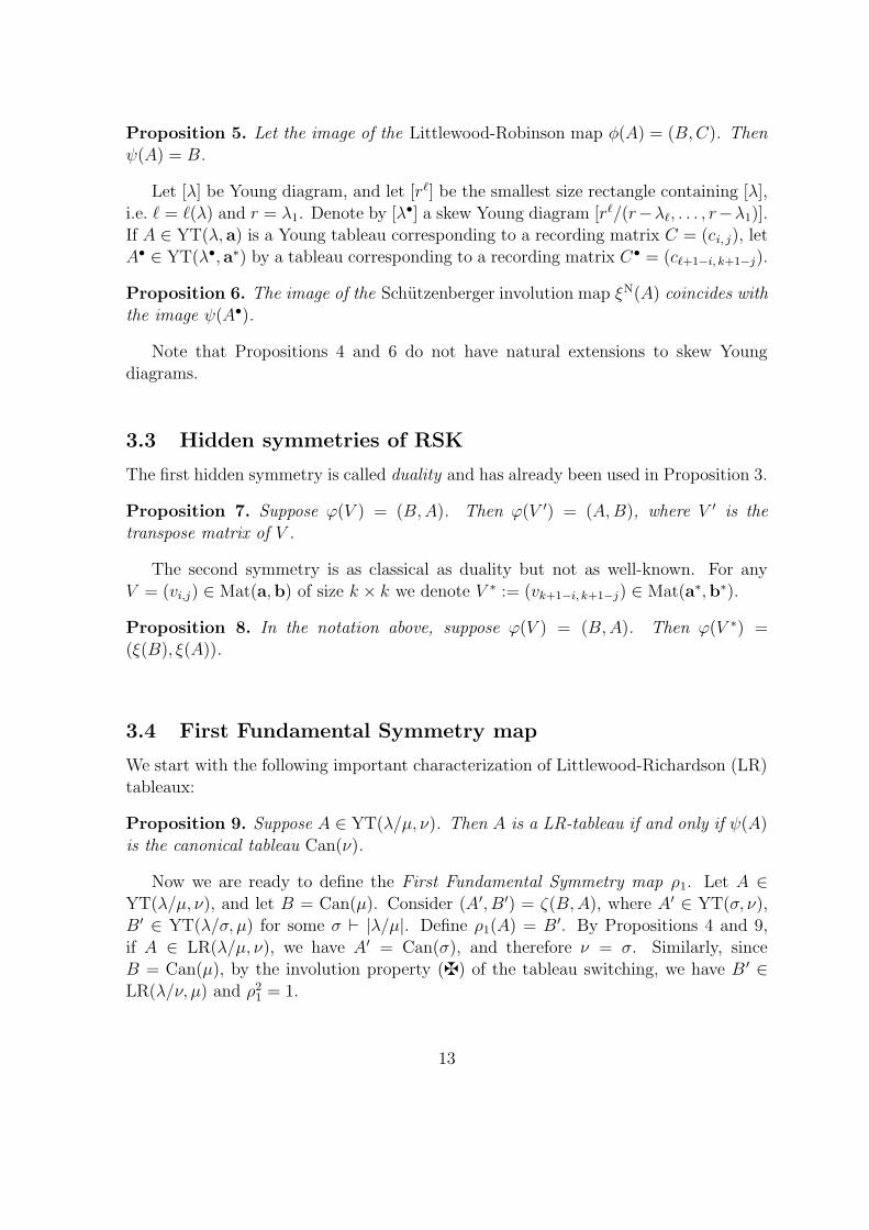
Now we are ready to define the First Fundamental Symmetry map ρ1. Let A ∈

YT(λ/µ, ν), and let B = Can(µ). Consider (A′, B′) = ζ(B,A), where A′ ∈ YT(σ, ν),B′ ∈ YT(λ/σ, µ) for some σ ` |λ/µ|. Define ρ1(A) = B′. By Propositions 4 and 9,if A ∈ LR(λ/µ, ν), we have A′ = Can(σ), and therefore ν = σ. Similarly, sinceB = Can(µ), by the involution property (z) of the tableau switching, we have B ′ ∈

LR(λ/ν, µ) and ρ21 = 1.

13

PSfrag replacements

A

B

C

A′

B′

C ′

λλ

µ

µ ν

νστ

ρ1

Figure 4: Illustration of ρ1 : A→ B′, where A ∈ LR(λ/µ, ν), B ′ ∈ LR(λ/ν, µ).

Proposition 10. The map ρ1 is well defined and gives a fundamental symmetry map.

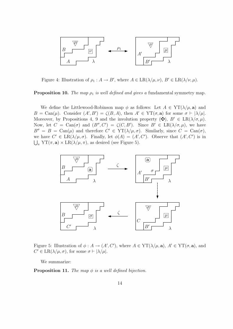
We define the Littlewood-Robinson map φ as follows: Let A ∈ YT(λ/µ, a) andB = Can(µ). Consider (A′, B′) = ζ(B,A), then A′ ∈ YT(σ, a) for some σ ` |λ/µ|.Moreover, by Propositions 4, 9 and the involution property (z), B ′ ∈ LR(λ/σ, µ).Now, let C = Can(σ) and (B ′′, C ′) = ζ(C,B′). Since B′ ∈ LR(λ/σ, µ), we haveB′′ = B = Can(µ) and therefore C ′ ∈ YT(λ/µ, σ). Similarly, since C = Can(σ),we have C ′ ∈ LR(λ/µ, σ). Finally, let φ(A) = (A′, C ′). Observe that (A′, C ′) is in⋃

π YT(π, a) × LR(λ/µ, π), as desired (see Figure 5).

PSfrag replacements

A

B

B

C

A′

B′

B′

C ′λλ

λλ

µ

µ

µ

µ

a

a

σ

σ

σ

τ

ζ

ζ

Figure 5: Illustration of φ : A → (A′, C ′), where A ∈ YT(λ/µ, a), A′ ∈ YT(σ, a), andC ′ ∈ LR(λ/µ, σ), for some σ ` |λ/µ|.

We summarize:

Proposition 11. The map φ is a well defined bijection.

14

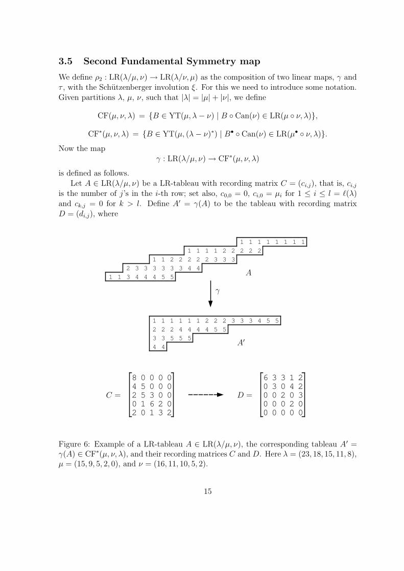
3.5 Second Fundamental Symmetry map

We define ρ2 : LR(λ/µ, ν) → LR(λ/ν, µ) as the composition of two linear maps, γ andτ , with the Schutzenberger involution ξ. For this we need to introduce some notation.Given partitions λ, µ, ν, such that |λ| = |µ| + |ν|, we define

CF(µ, ν, λ) = B ∈ YT(µ, λ− ν) | B Can(ν) ∈ LR(µ ν, λ),

CF∗(µ, ν, λ) = B ∈ YT(µ, (λ− ν)∗) | B• Can(ν) ∈ LR(µ• ν, λ).

Now the mapγ : LR(λ/µ, ν) → CF∗(µ, ν, λ)

is defined as follows.Let A ∈ LR(λ/µ, ν) be a LR-tableau with recording matrix C = (ci,j), that is, ci,j

is the number of j’s in the i-th row; set also, c0,0 = 0, ci,0 = µi for 1 ≤ i ≤ l = `(λ)and ck,j = 0 for k > l. Define A′ = γ(A) to be the tableau with recording matrixD = (di,j), where

1 1

2

3 4 4 4 5 5

3 3 3 3 3 3 4 4

1 1 2 2 2 2 2 3

21 1 1 2 2 2 2

3 3

1

1 1 1 1 1 1 1 1

84 52 5 30 1 6 20 1 3 22

60 30 0 20 0 0 20 0 0 00

3 3 1 20 4 20 30

4

4

2 2 2

3 3

1 1 1 1 1 1 22 2 3 3 3

5 5 5

5 5

4 4 4 5 5

4 4

0 0 0 00 0 00 00

PSfrag replacements

A

A′

C = D =

E =F =A′

B′

C ′

A′′

B′′

γ

λµ

aa∗

σξ

Figure 6: Example of a LR-tableau A ∈ LR(λ/µ, ν), the corresponding tableau A′ =γ(A) ∈ CF∗(µ, ν, λ), and their recording matrices C and D. Here λ = (23, 18, 15, 11, 8),µ = (15, 9, 5, 2, 0), and ν = (16, 11, 10, 5, 2).

15

di,j =

l−j∑

q=0

cl−j+i, q −

l−j+1∑

q=0

cl−j+1+i, q .

An example is given in Figure 6.

Proposition 12. The map γ is a well defined bijection.

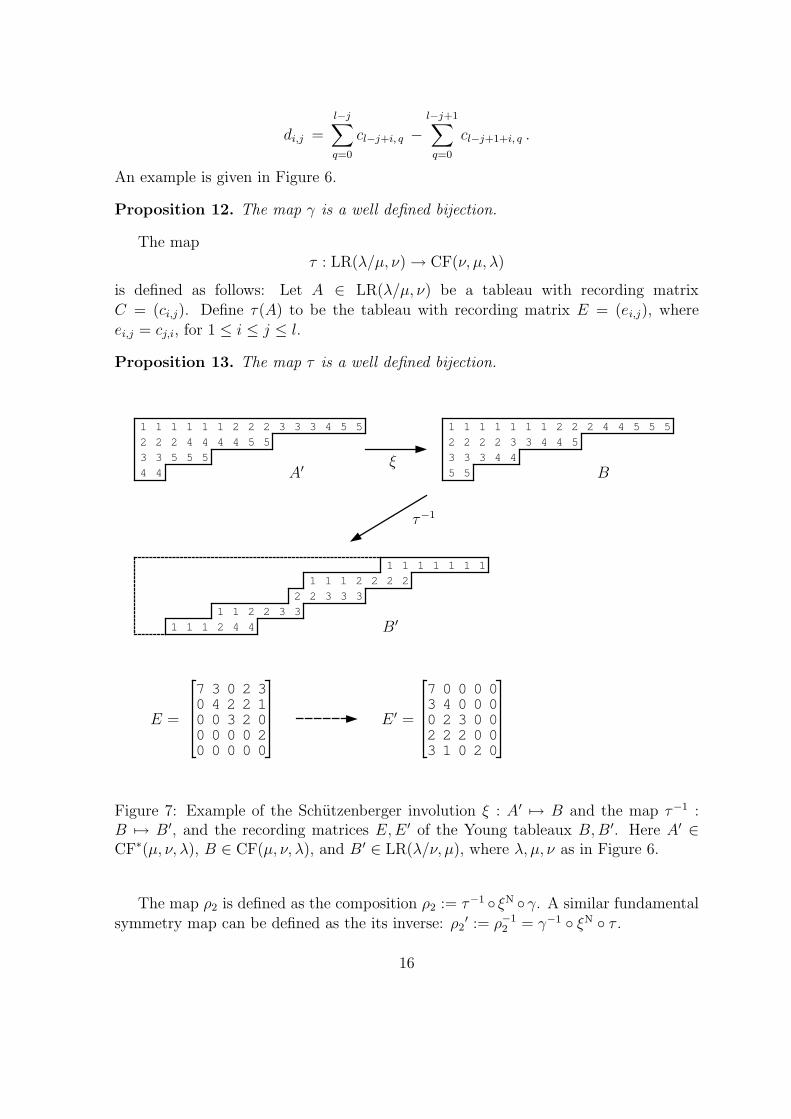
The mapτ : LR(λ/µ, ν) → CF(ν, µ, λ)

is defined as follows: Let A ∈ LR(λ/µ, ν) be a tableau with recording matrixC = (ci,j). Define τ(A) to be the tableau with recording matrix E = (ei,j), whereei,j = cj,i, for 1 ≤ i ≤ j ≤ l.

Proposition 13. The map τ is a well defined bijection.

1 1 2

3 3

4 4

1 1

2 2

2 2

3

21 1

1

2 2 2

3 3

1

1 1 1 1 1 1 1

73 40 2 32 2 2 01 0 2 03

0 0 0 00 0 00 00

74300

3 0 2 32 2 12 02

0 00 000000

0

4

4

2 2 2

3 3

1 1 1 1 1 1 22 2 3 3 3

5 5 5

5 5

4 4 4 5 5

4 4

2

5

2 2 2

3 3

1 1 1 1 1 1 21 2 2 4 4

3 4 4

5 5

3 3 4 4 5

5 5

PSfrag replacements

A A′

C =D =

E = E ′ =

A′

B

C ′ B′

B′′

C ′′

λµ

τ−1

ξ

Figure 7: Example of the Schutzenberger involution ξ : A′ 7→ B and the map τ−1 :B 7→ B′, and the recording matrices E,E ′ of the Young tableaux B,B ′. Here A′ ∈CF∗(µ, ν, λ), B ∈ CF(µ, ν, λ), and B ′ ∈ LR(λ/ν, µ), where λ, µ, ν as in Figure 6.

The map ρ2 is defined as the composition ρ2 := τ−1 ξN γ. A similar fundamentalsymmetry map can be defined as the its inverse: ρ2

′ := ρ−12 = γ−1 ξN τ .

16

Proposition 14. The maps ρ2 and ρ2′ are fundamental symmetry maps.

Note that, by Proposition 6 and the involution property (z), the restriction of theSchutzenberger involution defines a bijection ξN : CF∗(µ, ν, λ) → CF(µ, ν, λ). This,together with Propositions 12 and 13 imply Proposition 14.

We conjecture in Section 6.1 that ρ1 in fact coincides with ρ2 and with ρ2′. In the

absence of this result we use a different argument to prove linear equivalence of thesemaps and the remaining maps in Theorem 1.

3.6 Reversal

We define reversal as the conjugation of Schutzenberger involution with tableau switch-ing χ = ζ ξ ζ. More precisely, let A ∈ YT(λ/µ, a) and denote C = Can(µ). Consider(A′, C ′) = ζ(C,A) and (C ′′, A′′) = ζ(ξ(A′), C ′). Then, by Propositions 4, 9 and theinvolution property (z), C ′′ = Can(µ), and therefore A′′ ∈ YT(λ/µ, a∗). Reversal isdefined by χ(A) := A′′ (see Figure 8).

Proposition 15. The map χ is a well defined involution.PSfrag replacements

A

B

C

ξ(A′)

A′B′

C ′

C ′

A′′

B′′

C ′′

λλ

λλ

µ

µ

µ

µ

a

a

a∗

a∗

σ

ζ

ζ

ξ

Figure 8: Illustration of χ : A 7→ A′′, where A ∈ YT(λ/µ, a), A′′ ∈ YT(λ/µ, a∗).

17

4 Collection of linear reductions

4.1 Outline of the proof of Theorem 1

Following definitions, we would have to present 8 · 7 = 56 different linear reductions toprove Theorem 1. In fact, as will be shown in the next section, linear equivalence is anequivalence relation, so only 2 · (8 − 1) = 14 linear reductions suffice (say, between ϕand all other maps). Some of these reductions are quite difficult, while the proof canbe obtained by a smaller number of easier reductions. The latter follows a less obviouspattern summarized in the following lemma.

Recall that α → β stands for the map α linearly reducible to the map β.

Main Lemma For the maps as in Theorem 1, the following linear reductions hold:

• ϕ → ψ → φ → ζN → ξN → ϕ,

• ρ1 → ζN → ζ → ρ1 and ρ2 → ξN → ρ2,

• χ → ξN → χ.

In the next subsection we show that the Main Lemma implies the first part ofTheorem 1. The rest of the section will contain the proof of linear reductions in theMain Lemma.

4.2 Compositions of linear reductions

We start with the following elementary but very useful results, which simplify the proofof Theorem 1. While these results are standard in Computer Science, they have neverappeared in this context. We present short straightforward proofs for completeness.

Composition Lemma Suppose α1 → α2 and α2 → α3. Then α1 → α3. More-

over, if α1 can be computed in at most s1 cost of α2, and α2 can be computed in atmost s2 cost of α3, then α1 can be computed in at most (s1s2) cost of α3.

Proof. Suppose 1ג is a α2-based ps-circuit which computes α1, and 2ג is a α3-based ps-circuit which computes α2. Substitute each of the s(1ג) maps α2 in circuit 1ג

with the circuit .2ג Denote the resulting circuit by .ג By definition, ג is a α3-basedps-circuit computing α1. Observe also that α3 is used s(2ג) times in each copy of ,2גand thus α3 is used s(1ג)s(2ג) times in .ג This implies the result.

Corollary 1. Suppose α1 ∼ α2 and α2 ∼ α3. Then α1 ∼ α3.

Proof. By definition of linear equivalence, we have α1 → α2 → α3. Now theComposition Lemma implies α1 → α3. Similarly, α3 → α2 → α1, which implies α3 →

α1. We conclude α1 ∼ α3.

18

Corollary 2. (Cycle Lemma) Suppose α1 → α2 → . . . → αn → α1. Thenα1 ∼ α2 ∼ . . . ∼ αn.

Proof. For every 1 ≤ i < j ≤ n we have αi → αi+1 → . . . → αj and

αj → αj+1 → . . . → αn → α1 → α2 → . . . → αi .

By Composition Lemma, this implies αi → αj and αj → αi, and thus αi ∼ αj.

Corollary 3. Main Lemma implies the first part of Theorem 1.

Proof. By Cycle Lemma, we have ϕ ∼ ψ ∼ φ ∼ ζN ∼ ξN. These equivalences,ρ1 ∼ ζN ∼ ζ, ρ2 ∼ ξN, χ ∼ ξN and Corollary 1 prove the claim.

4.3 Reduction ϕ → ψ

The linear reduction of the RSK map ϕ to the Jeu de Taquin map ψ follows fromProposition 3. Below we present the corresponding ψ-based ps-circuit proving ϕ → ψ.

Input k, a,b, such that `(a), `(b) ≤ k. Input V = (vi,j) ∈ Mat(a,b). Set π := (a1 + · · · + ak, a1 + · · · + ak−1, . . . , a1). Set σ := (a1 + · · · + ak−1, a1 + · · · + ak−2, . . . , a1, 0). Set ρ := (b1 + · · · + bk, b1 + · · · + bk−1, . . . , b1). Set τ := (b1 + · · · + bk−1, b1 + · · · + bk−2, . . . , b1, 0). Set V l := (vk+1−i,j) ∈ Mat(a∗,b) and V ′l := (vj,k+1−i) ∈ Mat(b∗, a). Let Y ∈ YT(π/σ,b) be the tableau with recording matrix V l.

Compute B = ψ(Y ). Let X ∈ YT(ρ/τ, a) be the tableau with recording matrix V ′l.

Compute A = ψ(X). Output (B,A) = ϕ(V ).

The above circuit is a simple parallel circuit which uses ψ twice. To prove that itcomputes ϕ, apply Proposition 3.

4.4 Reduction ψ → φ

The linear reduction of the Jeu de Taquin map ψ to the Littlewood-Robinson map φfollows immediately from Proposition 5. The corresponding circuit is a trivial cir-cuit I(id, φ, δ), where id is the identity map, and δ is a projection onto the first com-ponent.

19

4.5 Reduction φ → ζN

The linear reduction of the Littlewood-Robinson map φ to the Tableau Switching mapfor normal shapes ζN follows from the definition of φ given before Proposition 11. Belowwe present the corresponding ζN-based ps-circuit proving φ → ζN.

Input k, a, partitions λ, µ, such that `(a), `(λ) ≤ k. Input A ∈ YT(λ/µ, a). Set B = Can(µ).

Compute (A′, B′) = ζN(B,A). Let σ be the shape of A′. Set C = Can(σ).

Compute (B′′, C ′) = ζN(C,B′). Output (A′, C ′) ∈ YT(σ, a) × LR(λ/µ, σ).

The above circuit is a simple sequential circuit which uses map ζN twice. Its correctnessfollows immediately from our definition of φ.

4.6 Reductions ζ → ξ and ζN → ξN

The linear reduction of the Tableau Switching map ζ to the Schutzenberger involution ξis given by the following simple sequential circuit.

Input k, µ ⊂ π ⊂ λ, a,b, such that `(λ), `(a), `(b) ≤ k. Input A ∈ YT(λ/π, a), B ∈ YT(π/µ,b).

Compute B′ = ξ(B) ∈ YT(π/µ,b∗), where b∗ = (bk, . . . , b1). Relabel integers in A by adding k to them. Let C := B′ ? A ∈ YT(λ/µ, (bk, . . . , b1, a1, . . . , ak)).

Compute C ′ = ξ(C) ∈ YT(λ/µ, (ak, . . . , a1, b1, . . . , bk)). Decompose C ′ := A′ ? B′′, where B′′ ∈ YT(λ/σ, b), A′ ∈ YT(σ/µ, a∗),

b = (0, . . . , 0, b1, . . . , bk), with k zeros, and σ ` |µ| + |a|. Relabel integers in B ′′ by subtracting k from them.

Compute A′′ = ξ(A′) ∈ YT(σ/µ, a). Output (A′′, B′′) = ζ(B,A).

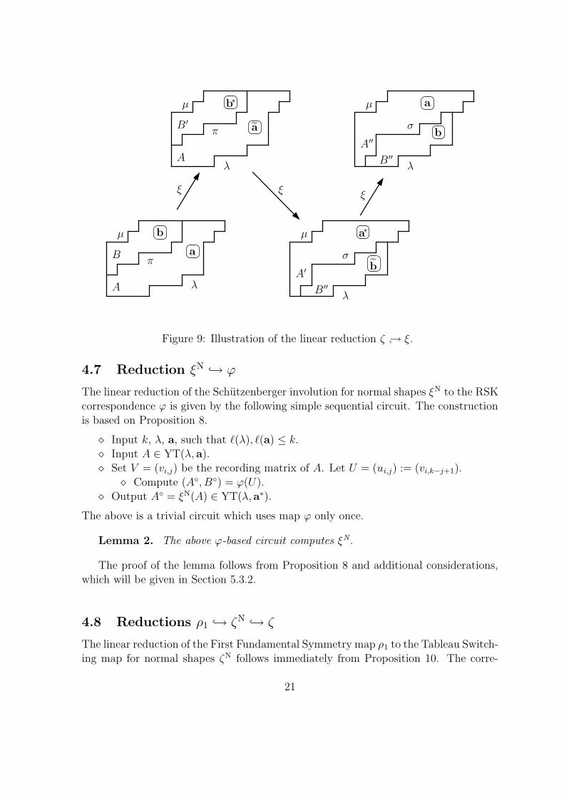
This gives a sequential circuit which uses ξ three times. We illustrate it in Figure 9.Here we use a = (0, . . . , 0, a1, . . . , ak), with k zeros and keep notation A,B ′′ for tableauxbefore and after relabelling. We hope this won’t lead to the confusion.

Lemma 1. The above ξ-based circuit computes ζ.

We postpone the proof till Section 5.3.1. The proof is based on Propositions 1 and 2in Section 3.1. When µ is the empty partition the above becomes a ξN-based circuitthat computes ζN.

20

PSfrag replacements

A

A

B

C

A′

B′C ′

A′′

B′′

B′′

C ′′

λ

λ

λ

λ

µµ

µµ

a

a

b

b

a

b

a∗

b∗

σ

σ

π

π

ξξ ξ

Figure 9: Illustration of the linear reduction ζ → ξ.

4.7 Reduction ξN → ϕ

The linear reduction of the Schutzenberger involution for normal shapes ξN to the RSKcorrespondence ϕ is given by the following simple sequential circuit. The constructionis based on Proposition 8.

Input k, λ, a, such that `(λ), `(a) ≤ k. Input A ∈ YT(λ, a). Set V = (vi,j) be the recording matrix of A. Let U = (ui,j) := (vi,k−j+1).

Compute (A, B) = ϕ(U). Output A = ξN(A) ∈ YT(λ, a∗).

The above is a trivial circuit which uses map ϕ only once.

Lemma 2. The above ϕ-based circuit computes ξN.

The proof of the lemma follows from Proposition 8 and additional considerations,which will be given in Section 5.3.2.

4.8 Reductions ρ1 → ζN → ζ

The linear reduction of the First Fundamental Symmetry map ρ1 to the Tableau Switch-ing map for normal shapes ζN follows immediately from Proposition 10. The corre-

21

sponding circuit is a trivial circuit I(δ1, ζ, δ2) where δ1 creates a canonical tableau B =Can(µ), ζ : (B,A) 7→ (A′, B′), and δ2 is a projection on the second component B ′. Weleave the easy technical details to the reader. The linear reduction ζN → ζ is trivial.

4.9 Reduction ζ → ρ1

This reduction is more involved than other linear reductions, and requires an interme-diate map ζLR. Formally, we first present a linear reduction ζ → ζLR, and then a linearreduction ζLR → ρ1. Now the Composition Lemma gives the desired construction.

4.9.1 Reduction ζ → ζLR

Suppose µ ⊂ λ, n = |λ/µ|, and |ν| + |τ | = n. Define LR-Tableau Switching to be aone-to-one correspondence:

ζLR :⋃

π `|λ|−|ν|

LR(π/µ, τ) × LR(λ/π, ν) −→⋃

σ `|λ|−|τ |

LR(σ/µ, ν) × LR(λ/σ, τ),

which is given by restriction of ζ to the sets as above.

Proposition 16. The map ζLR is a well defined bijection.

The reduction ζLR → ζ is trivial, but will not be needed. Below we show thatζ → ζLR, which implies that ζLR ∼ ζ.

We first describe the working of the reduction. Start with tableaux A, B andconsider a tableau (B ? A) C D, where C contains only integers as in A and Dcontains only integers as in B (see Figure 10). Let A := A s,0 C, B := B t,k D beparts of the tableau above, for some s, t, k to be defined; recall the definition of a,b

in Section 1. Clearly, tableau switching of A and B gives B′ t,k D, A′ s,0 C, where(A′, B′) = ζ(B,A). Now, if A s,0 C and B t,k D are LR-tableaux, this gives a linearreduction as desired. Below we show that one always find tableaux C, D as above.

Input k, µ ⊂ π ⊂ λ, c, d, such that `(λ), `(c), `(d) ≤ k. Input A ∈ YT(λ/π, c), B ∈ YT(π/µ,d). Set α := (c2 + · · · + ck, c3 + · · · + ck, . . . , ck, 0). Set β := (d2 + · · · + dk, d3 + · · · + dk, . . . , dk, 0). Set λ := (λ1 + α1 + β1, . . . , λ1 + α1 + βk, λ1 + α1, . . . , λ1 + αk, λ1, . . . , λk). Set π := (λ1 + α1 + β1, . . . , λ1 + α1 + βk, λ1, . . . , λ1, π1, . . . , πk). Set µ := (λ1 + α1, . . . , λ1 + α1, λ1, . . . , λ1, µ1, . . . , µk). Set A := A λ1,0 Can(α) ∈ LR(λ/π), B := B λ1+α1,k Can(β) ∈ LR(π/µ).

Compute (A′, B′) = ζLR(B, A). Decompose A′ = A′ λ1,0 Can(α), B′ = B′ λ1+α1,k Can(β), where

22

PSfrag replacements

A

B

CC

DD

A′

B′

C ′

A′′

B′′

C ′′

λλ

µµ

αα

ββ

cc d

d

σπ

ζLR

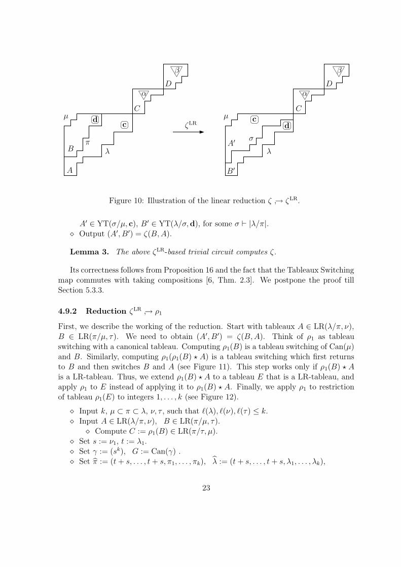
Figure 10: Illustration of the linear reduction ζ → ζLR.

A′ ∈ YT(σ/µ, c), B ′ ∈ YT(λ/σ,d), for some σ ` |λ/π|. Output (A′, B′) = ζ(B,A).

Lemma 3. The above ζLR-based trivial circuit computes ζ.

Its correctness follows from Proposition 16 and the fact that the Tableaux Switchingmap commutes with taking compositions [6, Thm. 2.3]. We postpone the proof tillSection 5.3.3.

4.9.2 Reduction ζLR → ρ1

First, we describe the working of the reduction. Start with tableaux A ∈ LR(λ/π, ν),B ∈ LR(π/µ, τ). We need to obtain (A′, B′) = ζ(B,A). Think of ρ1 as tableauswitching with a canonical tableau. Computing ρ1(B) is a tableau switching of Can(µ)and B. Similarly, computing ρ1(ρ1(B) ? A) is a tableau switching which first returnsto B and then switches B and A (see Figure 11). This step works only if ρ1(B) ? Ais a LR-tableau. Thus, we extend ρ1(B) ? A to a tableau E that is a LR-tableau, andapply ρ1 to E instead of applying it to ρ1(B) ? A. Finally, we apply ρ1 to restrictionof tableau ρ1(E) to integers 1, . . . , k (see Figure 12).

Input k, µ ⊂ π ⊂ λ, ν, τ , such that `(λ), `(ν), `(τ) ≤ k. Input A ∈ LR(λ/π, ν), B ∈ LR(π/µ, τ).

Compute C := ρ1(B) ∈ LR(π/τ, µ). Set s := ν1, t := λ1. Set γ := (sk), G := Can(γ) . Set π := (t+ s, . . . , t+ s, π1, . . . , πk), λ := (t+ s, . . . , t+ s, λ1, . . . , λk),

23

τ := (t, . . . , t, τ1, . . . , τk), all of length 2k. Set µ := (s+ µ1, . . . , s+ µk), κ := (s+ µ1, . . . , s+ µk, ν1, . . . , νk). Relabel the integers in A by adding k to them. Set C := C λ1,0 G ∈ LR(π/τ , µ), D := C ? A ∈ LR(λ/τ ,κ).

Compute E := ρ1(D) ∈ LR(λ/κ, τ). Set δ := (t, . . . , t) of length k, and τ = (0, . . . , 0, τ1, . . . , τk) of length 2k. Decompose E = F ? B′, where F ∈ LR(σ/κ, δ), B ′ ∈ YT(λ/σ, τ),σ = (t+ s, . . . , t+ s, σ1, . . . , σk) of length 2k, for some σ ` |λ/τ |.

Relabel the integers in B ′ by subtracting k from them: now B ′ ∈ LR(λ/σ, τ). Compute H := ρ1(F ) ∈ LR(σ/δ,κ).

Set ν = (0, . . . , 0, ν1, . . . , νk) of length 2k. Decompose H = (Can(µ) λ1,0 G) ? A′, where A′ ∈ YT(σ/µ, ν). Relabel the integers in A′ by subtracting k from them: now A′ ∈ LR(σ/µ, ν). Output (A′, B′) ∈ LR(σ/µ, ν) × LR(λ/σ, τ).

The above circuit is a sequential circuit which uses map ρ1 three times. Its correctnessis summarized in the following lemma.

Lemma 4. The above ρ1-based sequential circuit computes the restricted tableauxswitching map ζLR.

We prove the lemma in Section 5.3.4.

4.9.3 Using duality

One can use the duality (rotating the picture 180 degree and relabelling the integers)and apply ρ1 twice as in the beginning of the circuit above (in place of the the thirdapplication of ρ1). This gives a conceptually easier ρ1-based ps-circuit for ζLR, butwith a higher cost.

4.9.4 Reduction ζ → ζN

Note that it is not difficult to define directly a linear reduction ζ → ζN. Even thoughwe do not need this reduction, let us quickly outline it.

Let B ∈ YT(π/µ,d), A ∈ YT(λ/π, c) and C = Can(µ). Relabel the entries of Bby adding k to them, and compute (A′, D′) = ζN(C ? B,A). Decompose D′ = C ′ ? B′,where C ′ has content µ. Let σ be the shape of D′. Relabel the entries of B ′ bysubtracting k from them; thus B ′ ∈ YT(λ/σ,d). Let (C ′′, A′′) = ζN(A′, C ′). SinceC ′′ = Can(µ), we have that A′′ ∈ YT(σ/µ, c). We leave as an exercise to the interestedreader to show that (A′′, B′) = ζ(B,A). In this way we obtain a sequential ζN-basedcircuit which computes ζ.

24

PSfrag replacements

A

AA

B

C

C

D

G

A′

B′

D E

A

F

C ′

αβ

δ = (tk)

δkk

κ

κ

λλ

λλ

µ

µ

µµ

νν

νν

γ

π

ππ

στ

τ

τ

τ

τ

t

ρ1

ρ1

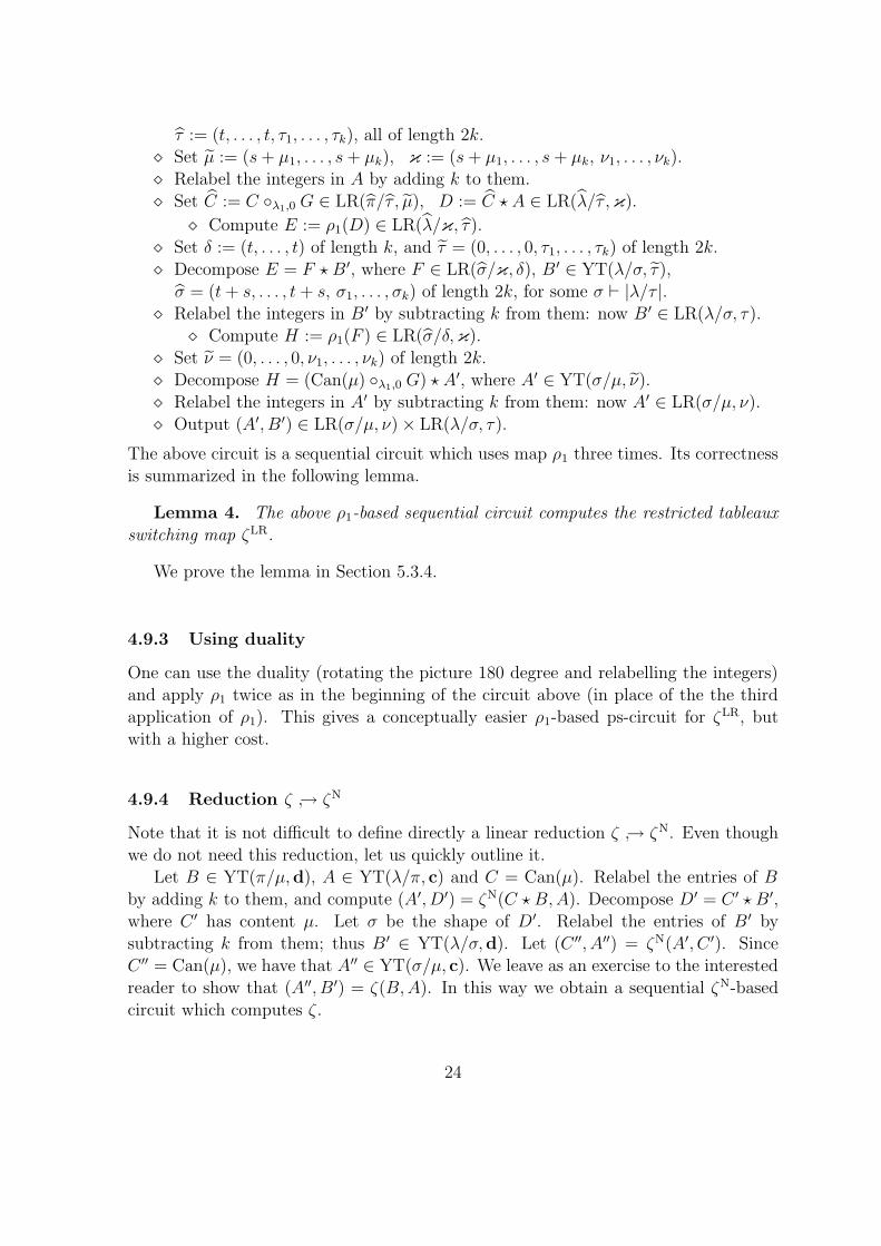
ss

Figure 11: Illustration of the first two applications of ρ1 in linear reduction ζLR → ρ1.

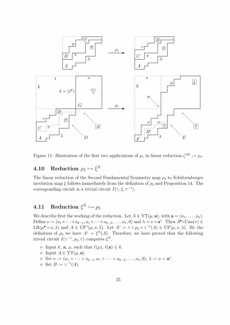
4.10 Reduction ρ2 → ξN

The linear reduction of the Second Fundamental Symmetry map ρ2 to Schutzenbergerinvolution map ξ follows immediately from the definition of ρ2 and Proposition 14. Thecorresponding circuit is a trivial circuit I(γ, ξ, τ−1).

4.11 Reduction ξN → ρ2

We describe first the working of the reduction. Let A ∈ YT(µ, a), with a = (a1, . . . , ak).Define ν = (a1+· · ·+ak−1, a1+· · ·+ak−2, . . . , a1, 0) and λ = ν+a∗. Then A•Can(ν) ∈LR(µ• ν, λ) and A ∈ CF∗(µ, ν, λ). Let A = τ ρ2 γ

−1(A) ∈ CF(µ, ν, λ). By thedefinition of ρ2 we have A = ξN(A). Therefore, we have proved that the followingtrivial circuit I(γ−1, ρ2, τ) computes ξN.

Input k, a, µ, such that `(µ), `(a) ≤ k. Input A ∈ YT(µ, a). Set ν := (a1 + · · · + ak−1, a1 + · · · + ak−2, . . . , a1, 0), λ := ν + a∗. Set B := γ−1(A).

25

PSfrag replacements

ABCD

G

A′

B′

A′

B′

H

F

C ′

αβ

δ = (tk)

δ

δ

k k

κ

λ

µ

µ

ν

ν

ν

γ

π

σσ

ττ

t

ρ1

s s

Figure 12: Illustration of the of the third application of ρ1 in linear reduction ζLR → ρ1.

Compute C := ρ2(B). Set A := τ(C). Output A = ξN(A) ∈ YT(µ, a∗).

4.12 Reduction ξN → χ

The reduction ξN → χ is trivial, since when µ = ∅, χ coincides with ξN.

4.13 Reduction χ → ξN

The linear reduction of the reversal map to the Schutzenberger involution for normalshapes is given by the following circuit.

Input k, µ ⊂ λ, a, such that `(λ), `(a) ≤ k. Input A ∈ YT(λ/µ, a). Set C := Can(µ).

Compute C := ξN(C) ∈ YT(µ, µ∗). Set c := (µk, . . . , µ1, a1, . . . , ak), d := (a1, . . . , ak, µ1, . . . , µk) of length 2k. Set µ := (0, . . . , 0, µ1, . . . , µk) of length 2k. Relabel de entries of A by adding k to them. Let B := C ? A ∈ YT(λ, c).

Compute B := ξN(B) ∈ YT(λ, c∗) Decompose B = A ? C ′, where A ∈ YT(ν, a∗), C ′ ∈ YT(λ/ν, µ) for some

partition ν ` |a|.

26

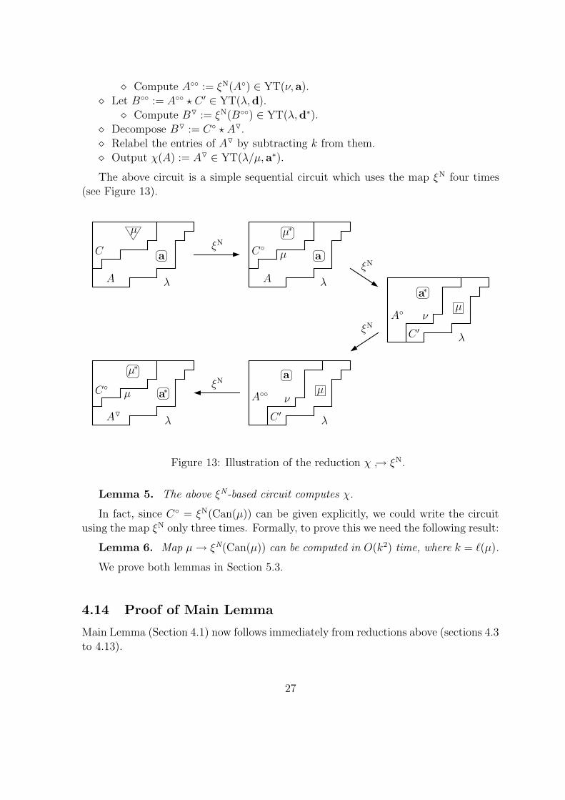
Compute A := ξN(A) ∈ YT(ν, a). Let B := A ? C ′ ∈ YT(λ,d).

Compute BO := ξN(B) ∈ YT(λ,d∗). Decompose BO := C ? AO. Relabel the entries of AO by subtracting k from them. Output χ(A) := AO ∈ YT(λ/µ, a∗).

The above circuit is a simple sequential circuit which uses the map ξN four times(see Figure 13).

PSfrag replacements

AA

B

C

ξ(A′)

A′

B′

C ′

C ′

C

C

A

A

AO

λ

λλ

λ

λ

µ

µ

µ

µ

µ

ν

ν

µ∗

µ∗

a

a

a

a∗

a∗

σ

ξN

ξN

ξN

ξN

Figure 13: Illustration of the reduction χ → ξN.

Lemma 5. The above ξN-based circuit computes χ.

In fact, since C = ξN(Can(µ)) can be given explicitly, we could write the circuitusing the map ξN only three times. Formally, to prove this we need the following result:

Lemma 6. Map µ→ ξN(Can(µ)) can be computed in O(k2) time, where k = `(µ).

We prove both lemmas in Section 5.3.

4.14 Proof of Main Lemma

Main Lemma (Section 4.1) now follows immediately from reductions above (sections 4.3to 4.13).

27

5 Proof of results

As we mentioned in the Introduction, there is an extensive literature in the subject ofYoung tableau bijections. Thus in many cases the technical results we need are alreadyknown. In the next subsection we give a brief overview the literature giving pointersto propositions. Readers interested in a modern treatment of the subject, completedefinitions and further references, are referred to [12, 36, 43]. An historic overview ofseveral of the constructions used here can be found in [26, 27]. The remainder of thissection contains proofs of lemmas and theorems.

5.1 Brief overview of the literature

The Schutzenberger involution or evacuation and the Jeu de Taquin were introduced byM.-P. Schutzenberger in his study of the combinatorics of Young tableaux [38, 40].The Schutzenberger involution is usually considered only in the case µ = ∅, but infact Schutzenberger extended this map to every poset [39]. Proposition 6 follows fromProposition 3 and the duality theorem in Appendix A1 in [12] or from Theorem A1.2.10in [43]. For Proposition 9 see [12, §5.2] or [43, A1.3.6]. An alternative extension of theSchutzenberger involution to skew shapes is the reversal map considered by Benkart,Sottile and Stroomer in [6, §5]. The reversal of a skew tableau can be characterizedby means of dual equivalence [16], although this is not the case for Schutzenbergerinvolution in the case of skew shapes. Proposition 15 is proved in §5 of [6] and followsfrom the fact that it is defined as the composition of three bijections and relations (z).

Bender-Knuth transformations were introduced by E. Bender and D.E. Knuthin their work on the enumeration of plane partitions [5]. Their connection withSchutzenberger involution was realized much later. Proposition 1 is explicit in [22,§2C], although it was probably discovered much earlier.

The RSK correspondence in full generality is due to Knuth [23], who built itbased on previous works of Robinson [35] and Schensted [37] (and conversations withSchutzenberger). Proposition 3 can be found in [40] or [45, §4] and Proposition 7in [23]. Proposition 8 appears in [24, Thm. D], [43, App. A] for standard tableaux,and in [12, App. A1] for tableaux of arbitrary weight.

Tableau switching, defined by means of the Bender-Knuth transformations, wasused by James and Kerber [21, §2.8] in a proof of the LR-rule. More recently, thetableau switching map was defined in a more general context in [6]; there its mainproperties were established. This is what we call the Tableau Switching map. See also[27, §2] for applications of tableau switching. Proposition 2 is Proposition 2.6 in [6],Proposition 4 is contained in [6, §2], and Proposition 16 is a part of Theorem 3.1 in [6].

The Littlewood-Robinson map (and other bijections of this type) remains littlestudied despite being one of the oldest Young tableau bijections. The first such mapwas defined by Robinson [35] in a different language in his effort to prove the LR-rule.

28

His proof was reworked by Macdonald in the first edition of [28, I9]. For a detailedaccount on Robinson’s paper see [27]; in Section 2.5 of this paper, van Leeuwen definesanother bijection of Littlewood-Robinson type using the Tableau Switching map. Thisbijection, given here in Section 3.3, is the one we call the Littlewood-Robinson map. Infact, van Leeuwen proves in [27] that this map coincides with the original one definedby Robinson and reworked by Macdonald. From the point of view of the LR-rulethis is unimportant, since any such bijection yields a proof of the LR-rule. Moreover,van Leeuwen shows using his definition that the Littlewood-Robinson map enjoys niceproperties, such as Proposition 5 in this paper and Corollary 2.5.2 in [27]. Proposition 5follows from Proposition 4, and Proposition 11 follows from Proposition 2 and therelations (z).

The problem of finding what we call a Fundamental Symmetry map appears to bepart of the ‘folklore’ of the are; it is very natural and has been considered independentlyby several investigators (see e.g. [2, 3, 7, 19]). Proposition 10 regarding our first map ρ1

is contained in [6, Example 3.6]. The Fundamental Symmetry maps ρ2 and ρ2′ are new

to our best knowledge. They are a byproduct of [32], and were motivated by Fulton’sappendix to [8]. More precisely, γ(A)• is the composition of the linear map Φl, betweenLR-triangles and hives, defined in [32, §4], with Fulton’s map in [8], or equivalentlythe composition of the linear map Ψl+1 Φl+1, between LR-triangles with last rowequal to zero and Berenstein-Zelevinsky triangles, defined in [32, §5], with Carre’smap in [11, §3]. Thus, Proposition 12 follows from [32] and Fulton [12] (which itselfis based on Carre’s work [11]). Note that both Carre and Fulton’s papers use setof tableaux CF∗(λ, µ, ν) to give combinatorial interpretations of LR-coefficients cλ

µ,ν ,which they connect to BZ-triangles and hives, respectively. In fact, the linear map γgives a simple combinatorial proof of cλµ,ν = |CF∗(λ, µ, ν)|; in this form it is new to thebest of our knowledge (cf. [32]).

The tableau τ(A) is called the companion tableau of A in [27, §1.4]. Proposition 13is equivalent to Proposition 1.4.3 there; its proof is straightforward. Proposition 14follows from Propositions 6, 12 and 13.

It is perhaps interesting to observe that the map Ψl Φl from LR-triangles to BZ-triangles, given in [32, §5], essentially contains γ and τ . More precisely, let A be aLR-tableau with LR-triangle (ai,j), and let Ψl Φl(ai,j) = (xi,j , yi,j , zi,j). Note thatthe recording matrix C = (ci,j) of A satisfies ci,j = aj,i. Suppose γ(A) = (di,j) andτ(A) = (ei,j), then di,j = xl−j+1, l−j+i and ei,j = yi,j−1 for all i < j. Besides, thenumbers di,i can be recovered from the di,j’s and the µj’s, and the numbers ei,i can berecovered from the ei,j’s and the νj’s. It should be noted that while ρ1 is an involution,we do not know whether ρ2 and ρ2

′ are, or equivalently, if ρ2 = ρ2′; but, see Conjecture 1

in Section 6.1.

29

5.2 Proof of relation (~)

Since, by relation (z) one has that tl, k = t−1k, l, it is enough to prove that

zk t−1k, l zl = zk+l .

This identity follows easily from the relations (♦) of the BK-transformations:

zk t−1k, l zl = [(s1)(s2s1) · · · (sk−1sk−2 · · · s2s1)] · [(sksk−1 · · · s2s1)(sk+1sk · · · s3s2)

(sk+2sk+1 · · · s4s3) · · · (sk+`−1sk+`−2 · · · s`+1s`)] · [(s1)(s2s1) · · · (s`−1s`−2 · · · s2s1)]

= [(s1)(s2s1) . . . (sk−1sk−2 · · · s2s1)] · [(sksk−1 · · · s2s1) (sk+1sk · · · s3s2)(s1)

(sk+2sk+1 · · · s4s3)(s2s1) · · · (sk+`−1sk+`−2 · · · s`+1s`)(s`−1s`−2 · · · s2s1)]

= (s1)(s2s1) · · · (sksk−1 · · · s2s1) · · · (sk+`−1sk+`−2 · · · s2s1) = zk+l .

Here the second equality follows from commuting parenthesized products in zl with thethe previous products in t−1

k, l.

5.3 Proof of lemmas

5.3.1 Proof of Lemma 1

Let k = `(B) and l = `(A). Use Propositions 1 and 2 to write Schutzenberger involutionand Tableau Switching up to relabelling as products of BK-transformations. In thenotation of Section 3.1, we need to prove that

tk, l = zl zk+l zk.

This follows from relations (z) and (~).

5.3.2 Proof of Lemma 2

Let A ∈ YT(λ, a) with recording matrix V = (vi,j). Then, by Proposition 3 forV l = (vk+1−i, j), we have ϕ(V l) = (A,−). Since V l∗ = (vi, k+1−j) = U , Proposition 8implies ϕ(U) = (ξN(A),−), and the claim follows.

5.3.3 Proof of Lemma 3

First, we need to show that A and B are both LR-tableaux. Indeed, since C is canonical,the integer (i) appears αi times in C, which is the total number of times (i+1) appearsin A. Therefore, when reading the word(A), the number of integers (i) is always atleast as many as the number of integers (i+ 1). By definition, this implies that A is aLR-tableau, and the same argument works for B.

30

Now observe that tableaux C and D remain unchanged under ζ. Furthermore,since ζLR is applicable and well defined, we easily see that action of ζLR restricted to(B,A) coincides with the action of ζ on (B,A). Indeed, simply observe that BK-transformations commute with taking compositions of tableaux. Thus, so do ele-ments tr, m−r and by Proposition 2, the Tableau Switching map ζ. Therefore, therestriction of ζLR to (B,A) coincides with ζ, which implies the result.

5.3.4 Proof of Lemma 4

We need the following property of tableau switching given in [6, Thm. 2.3]. Let(X,Y ) = ζ(U, V ?W ); then, there is an alternative way to calculate (X,Y ). Start with(V ′, U ′) = ζ(U, V ), and compute (W ′, U ′′) = ζ(U ′,W ). Then (X,Y ) = (V ′ ? W ′, U ′′).By the symmetry (z), the same “distributivity” property holds for (X ′, Y ′) = ζ(U ?

V,W ). During the proof we will adopt the following convention: if U and V aretableaux filled with integers 1, . . . , k then by U ?V we will denote the tableau obtainedby relabelling the entries of V by adding k to them, and then taking the union of Uand V (if this is possible).

Let (A,B) = ζ(B,A), and let A′, B′ be defined as in reduction 4.9.2. We have toshow that A = A′ and B = B′. Now, by Proposition 10, the map ρ1 is a special caseof the Tableau Switching map ζ. The first application of ζ computes (Can(τ), C) =ζ(Can(µ), B). The second application of ζ computes (Can(κ), B′) as the switching of(Can(τ), (C λ1,0 G) ? A). By decomposing Can(τ) as Can(δ) ?Can(τ), and Can(κ) asCan(µ) ? Can(ν) we obtain

() (Can(µ) ? Can(ν), F ? B ′) = ζ(Can(δ) ? Can(τ), (C λ1,0 G) ? A) .

Recall that tableau switching commutes with taking compositions (see Subsec-tion 5.3.3 above), and observe that Can(τ) lies to the left and below G. Now, bythe “distributivity” property, the second application of ζ starts with tableau switch-ing of Can(τ) and C, which is the inverse of the first application of ζ. The result-ing tableau B is then switched with A, giving B ′ as desired. The remaining stepsto be done according to the “distributivity” property as above do not change thetableaux B′ as it contains the largest integers k + 1, . . . , 2k. Therefore, B = B ′.The third application of ζ switches F with Can(µ) ? Can(ν), but according to (),Can(τ) switches first with (C λ1,0 G) ? A yielding (Can(µ) λ1,0 G) ? A,B); thenCan(δ) switches with (Can(µ) λ1,0 G) ? A yielding (Can(µ) ? Can(ν), F ). Thereforeρ1(F ) = (Can(µ) λ1,0 G) ? A, and restricting this tableau to the last k integers givesA = A′, as desired.

It remains to show that ρ1 is applicable the three times in the circuit. Since Bis already LR-tableau, the first application is valid. By Proposition 10, the resultingtableau C is also LR. We need to show that (Cλ1,0G)?A is LR-tableau. Since (Cλ1,0G)and A are already LR-tableau, all we need to show is that the number of (k + 1)’s is

31

always at most the number of k’s in a word. But that is clear since there are s = ν1

integers k in G, which all appear before the word reaches A. Finally, since F is obtainedby switching from Can(δ), it is a LR-tableau by Proposition 16. This justifies the thirdapplication of ρ1 and completes the proof of the lemma.

5.3.5 Proof of Lemma 5

Let A ∈ YT(λ/µ, a). We have to show that AO = χ(A). For this we will use thefollowing way of computing ξN(D) for a tableau D: Write D = E ? F , where E hasintegers 1, . . . , l, and F has integers l + 1, . . . , l + k. First compute ξ(E); then relabelthe entries of F by subtracting l from them, and compute (F ′, E) = ζ(ξ(E), F ).Finally, compute F = ξ(F ′), and relabel the entries of E by adding k to them. Weobtain ξ(D) = F ?E. This follows immediately from relations (~) in Section 3.1. NowB = ξN(B) is computed as follows: Observe that ξN(C) = C, let (A′, C ′) = ζ(C,A).Then, up to relabelling of C ′, we have B = ξN(A′)?C ′. By relation (z), we have A =A′. Thus B = A′?C ′. Finally, BO is obtained by taking (C ′′, A′′) = ζ(ξN(A′), C ′), andcomputing ξN(C ′′). Since C ′′ = C, ξN(C ′′) = C. Thus, up to relabelling, AO = A′′. Weclaim that A′′ = χ(A). Recall that by definition of the reversal map χ, the image χ(A)is the second component of ζ(ξ(A′), C ′). This implies the result.

5.3.6 Proof of Lemma 6

Let µ = (µ1, . . . , µ`), k := ` + 1, and set µk = 0. Compute a1,r := µk−r − µk−r+1, forall 1 ≤ r ≤ `, and ai,j := a1,j−i+1, for all 1 ≤ i ≤ j ≤ `. It is easy to see that (ai,j) isthe recording matrix of the desired tableau A = ξ(Can(µ)).

5.4 Proof of theorems

5.4.1 Proof of Theorem 1

As we showed in Section 4 (see Section 4.14 and Corollary 3), all the maps listed inTheorem 1 are linearly equivalent. To prove the second part of the theorem, let ussummarize all linear reductions in Figure 14. Here we draw an arrow for every linearreduction given by a ps-circuit ,ג and place the cost of the circuit s(ג) above the arrow.We do not to write the cost above trivial (cost 1) circuits.

Recall the second part of Composition Lemma which claims that one needs to takea product of costs when taking a composition of linear reductions. Now observe thatfrom each map in the diagram one can go to any other map (taking arrows in thereverse direction) so that the product never exceeds 36. This product maximizes whengoing from ρ1 to χ. The verification is straightforward and left to the reader.

32

PSfrag replacements

ϕ

ψ φ

ζN

ξN

ρ1

ζLR

ζ

ρ2χ

1

22

3

3

3

Figure 14: Diagram of linear reductions.

5.4.2 Proof of Theorem 2

Consider the map ξ. By Proposition 1, it can be computed at a cost of(

k2

)BK-

transformations. Each BK-transformation is a piecewise linear map which can becomputed at a cost of O(k) additions and max /min operations on integers ai,j . Notethat the size of integers ai,j never exceed λ1, so during and after all BK-transformationsthey have bit-size O(logm). Therefore, the total cost of computing ξ is O(k3 logm),as in the theorem. Also, by definition ξ is a size-neutral map (see Section 1.3).

By Theorem 1, all other maps are linearly reducible to ξN. Denote by α any ofthe remaining maps in Theorem 2, and by ג denote a ξN-based ps-circuit computing α(at a cost at most 36). Recall that ξN and all linear cost maps are size-neutral (seeSection 2.1), which makes map α size-neutral as well. Thus, the cost of computing anyof the (at most 36) maps ξN is O(k3 logm), where parameters k and logm are linearin the input parameters as in Theorem 2. Therefore, the total cost of computing α

following ג is O(k3 logm), as desired.

6 Further bijections

6.1 Third Fundamental Symmetry map

Here we present another Fundamental Symmetry map ρ3, defined in [2, 3]. The def-inition in these papers is somewhat convoluted so we restate it here for the sake ofclarity.

Start with LR-tableau A ∈ LR(λ/µ, ν). Fill shape [µ] with zeros. We remove rowsone by one, beginning with the bottom row. In each row to be removed, build a chain ofintegers in previous rows, starting with the last element and going to the first element.For each such element x, find the largest element y < x in the previous row, not used

33

by the previous chains (starting from row containing x), then the largest element z < yin the row above that of y not used by the previous chains, etc. Now replace y with x, zwith y, etc. unless the integer k goes in < k-th row; stay put in that case. Note thateach zero forms a chain of length 1.

Denote by vi,j the number of chains of length (i− j + 1) which start from i-th row.Let B ∈ YT(λ/ν, µ) be a Young tableau corresponding to recording matrix V = (vi,j).We claim that B is a LR-tableau, and define B = ρ3(A).

1

1

1

1 1

2 2

2 2

3

1

1

1

1 1

2 2

2 2

3

0 0 0 0 0 0 0

00 00

0

0

0

0 0

0

2

2

1 1

2 3

0 0 0 0 0 1

10 00

21

0

0

0

0

10

0

0 0 0 11

221 2

0

0 2

1

0 10 00 1 1 1 1

4111

23

211

1

1

1

1

1 1

2

2 2 2

3

1 1

2 2

3

3

4

PSfrag replacements

A B

V =

ρ3

Figure 15: An example of the map ρ3 : A→ B, where A ∈ LR(λ/µ, ν), B ∈ LR(λ/ν, µ),and λ = (9, 7, 6, 5), µ = (7, 6, 3, 1), ν = (5, 4, 1). There is one chain of length 4, 3, 1,and two chains of length 2, starting from the 4-th row (see 4-th row of V ).

Conjecture 1. The Fundamental Symmetry maps ρ1, ρ2, ρ2′ and ρ3 are identical.

The conjecture is supported by numerical evidence. Also, in [3, §5] it was shownthat (ρ3)

2 = 1 by an involved argument. If established, the conjecture would simplify

34

the proof of Theorem 1 and further emphasize the importance of the fundamentalsymmetry.

6.2 Inverse maps

Recall that maps ϕ and φ are one-to-one.

Conjecture 2. The RSK map ϕ and the Littlewood-Robinson map φ are linearlyequivalent to their inverses.

Let us emphasize here the need to distinguish between direct and inverse maps. Itis a well known and studied phenomenon in Cryptography that some maps are easilycomputed, while their inverses are not; taking powers over the finite field vs. takingdiscrete logarithm being the most celebrated example. The conjecture above saysthere is no such problem with Young tableau maps and all Young tableau bijectionsare linearly equivalent to their inverses. Note that Schutzenberger involution, TableauSwitching, Reversal and the First Fundamental Symmetry maps are equal to theirinverses (z), and if Conjecture 1 holds so is the Second Fundamental Symmetry map.Thus the problem makes sense only for RSK and Littlewood-Robinson maps, as in theconjecture.

6.3 Octahedral map

Suppose four partitions λ, µ, ν, and τ satisfy |τ | = |λ|+ |µ|+ |ν|. The Octahedral mapis a one-to-one correspondence:

ς :⋃

σ `|λ|+|µ|

LR(σ/λ, µ) × LR(τ/σ, ν) −→⋃

π `|µ|+|ν|

LR(π/µ, ν) × LR(τ/λ, π).

A bijection of this type was introduced in [25], in the equivalent language of hives, asa tool for a new proof of the LR-rule. This is defined using an octahedral recurrence

considered earlier in connection with the enumeration of alternating sign matrices [34],and has recently appeared in other context [19, 42, 46].

As it was the case with the Littlewood-Robinson map, the existence of any suchbijection ς will suffice in the proof of the LR-rule given in [25]. So, we will define analternative version of the octahedral map using the tableau switching map ζ. From ourpoint of view, this has the advantage that the definition given here yields the reductionς → ζ.

We define an Octahedral map ς as follows: Let A ∈ LR(σ/λ, µ), B ∈ LR(τ/σ, ν).Consider (A′, C ′) = ζ(Can(λ), A); since A is a LR tableau, A′ = Can(µ) and C ′ ∈

35

LR(σ/µ, λ). Next, let (B ′, C ′′) = ζ(C ′, B). Again, since switching preserves the prop-erty of being a Littlewood-Richardson tableau, there is some partition π of |µ| + |ν|,such that B ∈ LR(π/µ, ν) and C ′′ ∈ LR(τ/π, λ). Finally, let (C ′′′, D) = ζ(Can(π), C ′′).Thus, C ′′′ = Can(λ) and D ∈ LR(τ/λ, π). We define ς(A,B) = (B ′, D).

The following proposition is a consequence of (z).

Proposition 17. The map ς defined above is a bijection.

Corollary 4. The Octahedral map ς is linearly reducible to Tableau Switching map ζ

and other maps in Theorem 1.

Note that ς is defined by a simple sequential circuit which uses the map ζ threetimes; thus ς → ζ. Another way to prove this is to show first that ς is a compositionof the LR-Tableau Switching map ζLR and the fundamental symmetry maps. Let usconclude this section with the following natural conjecture:

Conjecture 3. The map ς and the map defined in [25] are identical and linearly

equivalent to maps in Theorem 1.

We should mention that the connection between Tableau Switching map ζ andthe Octahedral map in [25] follows from [18] through linear equivalence with the Jeude Taquin map ψ. Also, it was shown in [19] that in a special case the map ς givesa (another version) fundamental symmetry map (see the “commutor” in Section 5.2of [19]). It is natural to conjecture that this fundamental symmetry map coincideswith ρ1 as well.

6.4 Burge correspondence

Let ϕ denote the Burge correspondence [9] (see also [12, A4.1]). Numerically, it definesa one-to-one map between the same sets as the RSK map ϕ :

ϕ : Mat(a,b) −→⋃

λ`N

YT(λ,b) × YT(λ, a)

This bijection is related to RSK correspondence in the following way. Let V = (vi,j);denote V l := (vk+1−i,j) and V ↔ := (vi,k+1−j). Let ϕ(V ) = (B,A). Then, since columninsertion commutes with row insertion [12, A2], we have that ϕ(V l) = (B, ∗) andϕ(V ↔) = (∗, A). Thus ϕ → ϕ and this is done by a ϕ-based simple parallel circuitwhich uses ϕ twice. Similarly, one can show that ϕ → ϕ, which implies ϕ ∼ ϕ.

36

6.5 Hillman-Grassl map

Let λ ` n be a fixed partition, ` = `(λ), m = λ1. For every function F : [λ] → Z≥0

and every −` < c < m, define diagonal sums

αc(F ) =∑

(i,j)∈[λ], j−i=c

F (i, j),

and rectangular sums

βc(F ) =ic∑

i=1

jc∑

j=1

F (i, j),

where (ic, jc) is the last square on the diagonal j− i = c. Now, let d = (d1−`, . . . , dm−1)be a nonnegative integer array. Define Bd to be sets of all nonnegative integer func-tions F as above, such that βc(F ) = dc, for all −` < c < m. Similarly, define Ad to besets of all reverse plane partitions of shape λ, such that αc(F ) = dc, for all −` < c < m.

The Hillman-Grassl (HG) bijection defines a one-to-one map ϑλ : Bd → Ad [20](see also [13, 15, 29]). It is easy to check that when λ = (kk) the set Bd coincideswith Mat(a,b) for certain a,b, while Ad corresponds to pairs of GT-patterns joinedat the diagonal [29]. In [13, Thm. 10.2] Gansner showed that the map ϑk := ϑλ inthis case coincides, up to a linear cost map, with the Burge correspondence ϕ. Thisimmediately gives ϑk ∼ ϕ. Combining this equivalence with the one in the previoussection we conclude that the HG-map in the “square case” is linearly equivalent to theRSK correspondence ϑk ∼ ϕ, as well as all other maps listed in Theorem 1. We omitthe (easy) details.

For general shapes λ, given F ∈ Ad, set k := maxm, `, and fill with zeros therest of the k×k square containing [λ]. Now apply RSK map ϕ to the resulting matrix.At the end, join at the diagonal the two GT-patterns of the resulting tableaux, andrestrict this function to squares in [λ] (see [29] for details). We leave it to the readerto show that this defines linear reduction ϑλ → ϕ, proving linear equivalence ϑλ ∼ ϕin general case, where λ is a part of the input.

To conclude, we note that the connection of ϑ with BK-transformations was ob-served in [29], where it was also shown that ϑ can be computed in O(k3 logm), wherem = maxcdc.

6.6 Other symmetry maps

Beside fundamental symmetry maps, there is a large number of “hidden” symmetriesof Littlewood-Richardson coefficients cλµ,ν . These symmetries form a finite group andwere studied on a number of occasions (see [7]). As we mentioned above, a subgroupof index 2 of these symmetries can be given by linear cost maps [32]. Since the funda-mental symmetry is a remaining generator, the symmetries outside this subgroup aregiven by maps which are all linearly equivalent to ρ1.

37

A different kind of symmetry map was given in [17] (see also [1, §3]):

% : LR(λ/µ, ν) −→ LR(λ′/µ′, ν ′),

where λ′ denotes the conjugate diagram (reflected across i = j line). The bijectionsgiven in [17, 1] use a modified insertion map. It would be interesting to see whetherthis symmetry map is linearly equivalent to maps we consider in Theorem 1.

6.7 Schutzenberger involution

Recall that we have not been able to show that the general Schutzenberger involution ξreduces to the other bijections appearing in this paper, while we were able to showthat ξN and χ do. If ξ were not reducible to the other bijections this would mean thatχ is a more natural extension of ξN to skew shapes than ξ. Recall [6, §5] that reversalis also more natural than Schutzenberger involution from the point of view of dualequivalence. Proving that ξ is reducible to ξN remains an open problem.

7 Final Remarks

1. Note that we never attempted to give a lower bound on the complexity of the costof tableau bijections. Since all constructions require θ(k2) min-max operations, it isconceivable that such lower bound can be obtained by means of Algebraic ComplexityTheory [10]. In other words, if one properly restrict the class of algorithms to consider,the lower bound Ω(k3) might be attainable. Further investigation of this matter wouldbe of great interest.

2. While the Octahedral map defined in [25] (see also [19]) looks extremely natural,it lacks formal and complete treatment in combinatorics literature. Our alternativeversion of this map and Conjecture 3 is a further indication of this. We would like toencourage the reader to further study this map and its connections to other combina-torial maps.

3. There are a score of other notable Young tableau bijections not mentioned in thepaper. While some of these are based on some kind of insertion/evacuation proceduresand thus seem strongly related to the maps we study, others are of a different nature.Examples of the first type include Lascoux-Schutzenberger action of Sm on YT(λ/µ;m),RSK for shifted and super tableaux, etc. Examples of the second type include theNovelli-Pak-Stoyanovskii’s bijection, and nonintersecting paths arguments. We referto [12, 36, 43] for definitions and references. It would be nice to place these maps intoour framework and perhaps even introduce some kind of complexity style hierarchy onthem.

38

4. In [6] the authors present an important characterization of the tableau switchingthrough its natural properties. In principle, one can use our linear reductions to obtainsimilar characterizations of the fundamental symmetry maps. We challenge the readerto make such a characterization explicit. This could lead to a positive resolution ofConjecture 1 and give a better understanding of the subject.

5. It was noted in [29] that the Hillman-Grassl map extends to real-valued func-tions and is given by a continuous piecewise-linear volume-preserving map in this case.Similar observations were made for other sets of Young tableaux and other tableaubijections (see e.g. [2, 7, 22, 32]). One can check that most of our linear reductionsalso extend to real-valued tableaux, and our linear cost maps are in fact (the usual,geometric) linear maps. Thus, one “real extension” suffice to establish the others. Weleave further exploration of this subject to the interested reader.

6. We make no effort to optimize the constant 36 in the proof of Theorem 1. In fact,if ρ1 = ρ2 as Conjecture 1 suggests, this constant immediately drops down to 12. Wewanted to emphasize the existence of such a constant, and would be just as happy ifit worked out to be around 200, as in the first draft of the paper.

The idea to study the cost as the number of “large operations” is well-known inComputer Science literature. It was rejected for the purposes of Cryptography after A.Shamir showed in [41] that factoring has a polynomial cost algorithm in the numberof arithmetic operations (of possibly very large integers). In our situation, all mapsare size-neutral, so this problem never arises. Still, we should warn the reader that theconstant implied by the O(·) notation in Theorem 2 is much larger than 36.

7. It was noticed in [31] that there is a certain uniqueness behind the linear costpartition bijections. This method was later used in [32] to obtain several linear costLR-symmetry maps. We wonder if there is an “automatic” procedure to define themaps in Theorem 1. Even a framework for that would be of great interest.

8. We conclude by saying that even though we were able to formalize the connectionsbetween Young tableau bijections, this is important on a computational and perhapsphilosophical level, but is hardly an “explanation from the Book”. We firmly believethat the real underlying structure behind these connections lies in the study of canonicalbases in representation theory of symmetric and full linear groups.

Acknowledgements

We are grateful to Olga Azenhas, Arkady Berenstein, Andre Henriques, Leonid Levin,Ezra Miller, Richard Stanley and Terry Tao for interesting conversations and helpfulremarks. Special thanks to David Jackson for reading and editing the previous versionof the paper and his meticulous attention to details.

39

The first author was supported by the NSA and the NSF. Part of this work was doneduring second author’s sabbatical stay at MIT Mathematics Department. The secondauthor would like to thank CONACYT and DGAPA-UNAM for financial support, andto Richard Stanley for his support in the realization of the visit. The second authorwas also partially supported by DGAPA-UNAM IN111203. The first author wouldalso like to thank the second author for organizing his visit to Mexico, where this workwas continued.

References

[1] O. Azenhas, The admissible interval for the invariant factors of a product of matrices,Linear and Multilinear Algebra 46 (1999), 51–99.

[2] O. Azenhas, Littlewood-Richardson fillings and their symmetries, in Matrices and Group

Representations, Textos de Matematica, Serie B 19 (1999), Depto. de Matematica, Univ.de Coimbra, 81–92.

[3] O. Azenhas, On an involution on the set of Littewood-Richardson tableaux andthe hidden commutativity, preprint, 2000, available from http://dingo.mat.uc.pt/

cmuc/publicline.php?lid=1

[4] A. Barvinok and S. Fomin, Sparse interpolation of symmetric polynomials, Adv. Appl.

Math. 18 (1997), 271–285.

[5] E. A. Bender and D. E. Knuth, Enumeration of plane partitions, J. Combin. Theory,Ser. A 13 (1972), 40–54.

[6] G. Benkart, F. Sottile and J. Stroomer, Tableau switching: algorithms and applications,J. Combin. Theory, Ser. A 76 (1996), 11–43.

[7] A. D. Berenstein and A. Zelevinsky, Triple multiplicities for sl(r+1) and the spectrum ofthe exterior algebra of the adjoint representation, J. Algebraic Combin. 1 (1992), 7–22.

[8] A. Buch, The saturation conjecture (after A. Knutson and T. Tao), Enseign. Math. 46

(2000), 43–60.

[9] W. H. Burge, Four correspondences between graphs and generalized Young tableaux, J.

Combin. Theory, Ser. A 17 (1974), 12–30.

[10] P. Burgisser, M. Clausen and M. A. Shokrollahi, Algebraic Complexity Theory, Grund-lehren der mathematischen Wissenschaften, Vol. 315, Springer, Berlin, 1997.

[11] C. Carre, The rule of Littlewood-Richardson in a construction of Berenstein-Zelevinsky,Internat. J. Algebra & Comput. 1 (1991), 473–491.

[12] W. Fulton, Young Tableaux, L.M.S. Student Texts 35, Cambridge U. Press, 1997.

40

[13] E. R. Gansner, Matrix correspondences of plane partitions, Pacific J. Math. 92 (1981),295–315.

[14] M. R. Garey and D. S. Johnson, Computers and intractability: A guide to the theory of

NP-completeness, Freeman, New York, 1979.

[15] R. M. Grassl and A. P. Hillman, Functions on tableau frames, Discrete Math. 25 (1979),245–255.

[16] M. D. Haiman, Dual equivalence with applications, including a conjecture of Proctor,Discrete Math. 99 (1992), 79–113.

[17] P. Hanlon and S. Sundaram, On a bijection between Littlewood-Richardson fillings ofconjugate shape J. Combin. Theory, Ser. A 60 (1992), 1–18.

[18] A. Henriques and J. Kamnitzer, On the symmetric monoidal category constructed usingthe octahedral recurrence, preprint, 2003.

[19] A. Henriques and J. Kamnitzer, The octahedron recurrence and gLn crystals, Proc.

16-th FPSAC Conf., Vancouver, BC, 2004, available from http://www-math.mit.edu/

˜andrhenr/.

[20] A. P. Hillman and R. M. Grassl, Reverse plane partitions and tableau hook numbers, J.

Combin. Theory, Ser. A 21 (1976), 216–221.

[21] G. D. James and A. Kerber, The Representation Theory of the Symmetric Group, En-cyclopedia of Mathematics and its Applications 16, Addison-Wesley, Reading, Mas-sachusetts, 1981.

[22] A. N. Kirillov and A. D. Berenstein, Groups generated by involutions, Gelfand-Tsetlinpatterns, and combinatorics of Young tableaux, St. Petersburg Math. J. 7 (1996), 77–127.

[23] D. E. Knuth, Permutations, matrices and generalized young tableaux, Pacific J. Math.

34 (1970), 709–727.

[24] D. E. Knuth, The Art of Computer Programming, vol. 3, Sorting and Searching, seconded., Addison-Wesley, Reading, Massachusetts, 1998.

[25] A. Knutson, T. Tao and C. T. Woodward, A positive proof of the Littlewood-Richardsonrule using the octahedron recurrence, arXiv:math.CO/0306274.

[26] M. A. A. van Leeuwen, The Robinson-Schensted and Schutzenberger algorithms, anelementary approach, Electron. J. Comb. 3 (1996), RP R15, 32 p.

[27] M. A. A. van Leeuwen, The Littlewood-Richardson rule, and related combinatorics, inInteraction of combinatorics and representation theory, 95–145, MSJ Mem. 11, Math.Soc. Japan, Tokyo, 2001.

[28] I. G. Macdonald, Symmetric functions and Hall polynomials, second ed., Oxford Uni-versity Press, Oxford, 1995.

41

[29] I. Pak, Hook length formula and geometric combinatorics, Semin. Lothar. Comb. 46,B46f (2001), 13 pp.

[30] I. Pak, Partition Bijections, a Survey, to appear in Ramanujan Journal, available fromhttp://www-math.mit.edu/˜pak.

[31] I. Pak, Partition Identities and Geometric Bijections, Proc. A.M.S., to appear, 2003.

[32] I. Pak and E. Vallejo, Combinatorics and geometry of Littlewood-Richardson cones, toappear in Europ. J. Comb., available from http://www-math.mit.edu/˜pak.

[33] C. H. Papadimitriou, Computational Complexity, Addison-Wesley, Amsterdam, 1994.

[34] D. P. Robbins and H. Rumsey, Determinants and alternating-sign matrices. Adv. Math.

62 (1986), 169–184.

[35] G. de B. Robinson, On the representations of the symmetric group, Amer. J. Math. 60

(1938), 745–760.

[36] B. E. Sagan, The symmetric group. Representations, combinatorial algorithms, and sym-

metric functions, second ed., Graduate Texts in Mathematics 203, Springer, New York,2001.

[37] C. Schensted, Longest increasing and decreasing subsequences, Canad. J. of Math. 13

(1961), 179–191.

[38] M.-P. Schutzenberger, Quelques remarques sur une construction de Schensted, Math.

Scand. 12 (1963), 117–128.

[39] M.-P. Schutzenberger, Promotion des morphismes d’ensembles ordonnes, Discrete Math.

2 (1972), 73–94.

[40] M.-P. Schutzenberger, La correspondance de Robinson, in Combinatoire et Repre-

sentation du Groupe Symetrique, Lecture Notes in Math. 579, Springer, 1977, 59–135.

[41] A. Shamir, Factoring Numbers in O(log n) Arithmetic Steps, Inf. Proc. Letters 8 (1979),28–31.

[42] D. E. Speyer, Perfect Matchings and the Octahedron Recurrence, arXiv:math.CO/0402452.

[43] R. P. Stanley, Enumerative Combinatorics, vol. 2, Cambridge Studies in Advanced Math-ematics 62, Cambridge University Press, 1999.

[44] J. R. Stembridge, Computational aspects of root systems, Coxeter groups, and Weylcharacters, in Interaction of combinatorics and representation theory, 1–38 , MSJ Mem.

11, Math. Soc. Japan, Tokyo, 2001.

[45] G. P. Thomas, On a construction of Schutzenberger, Discrete Math. 17 (1977), 107–118.

[46] D. Thurston, From Dominoes to Hexagons, arXiv:math.CO/0405482.

42