
Ship Resistance Simulations with OpenFOAM - OpenFOAM Workshop
Reduction of Ship Resistance through Induced Turbulent Boundary Layers
by
Kevin Joseph Donnelly
Bachelors of Science
Ocean Engineering
Florida Institute of Technology
2009
A thesis
submitted to the Florida Institute of Technology
in partial fulfillment of the requirements
of the degree of
Master of Science
in
Ocean Engineering
Melbourne, Florida
December, 2010

© Copyright 2010 Kevin Joseph Donnelly
All Rights Reserved

We the undersigned committee
hereby approve the attached thesis
Reduction of Ship Resistance through Induced Turbulent Boundary Layers
by
Kevin Joseph Donnelly
_________________________________
Prasanta K. Sahoo, Ph. D
Associate Professor of Ocean Engineering
Marine and Environmental Systems
Major Advisor
_________________________________
Stephen Wood, Ph. D, PE
Assistant Professor and Program Chair of Ocean Engineering
Marine and Environmental Systems
Committee Member
_________________________________
Chelakara Subramanian, Ph. D, PE, FIIE
Professor and Program Chair
Mechanical and Aerospace Engineering
Outside Member
_________________________________
George A. Maul, Ph. D
Professor of Oceanography
Marine and Environmental Systems
Department Head
iii
ABSTRACT
Reduction of Ship Resistance through Induced Turbulent Boundary Layers
by
Kevin Joseph Donnelly
Major Advisor: Dr. Prasanta K. Sahoo
In this research, the resistance of dimpled hull forms and their potential relevance
in reducing the resistance of modern conventional hull forms has been investigated.
This research has been undertaken while trying to understand the flight dynamics
of a dimpled golf ball. Non-streamlined bodies, like spheres, have significant
pressure drag due to flow separation. Pressure drag can be reduced through
separation delay. The flow around a sphere with a Reynolds number less than
3x10⁵ has a laminar boundary layer, thus the flow would separate at an angle of 82
o
relative to the stagnation point. If the Reynolds number is increased beyond 3x10⁵
the boundary layer becomes turbulent and separation occurs at 125o. It is
understood that dimples are placed on a golf ball to trip the boundary layer from
laminar to turbulent in order to delay flow separation. It is believed that the same
concept can be adapted for use on a ship to decrease viscous resistance. Two model
boats were created, a control (an unmodified model) and the experiment hull (one
modified with dimples). Based on the experimental investigations, it cannot be
determined if the reduction of ship resistance through induced turbulent boundary
layers was a success for this hull form; however, it can be concluded that it was not
a failure. Stochastically speaking, based on the quantitative magnitude of the
resistance measurements taken, 0.032 kg (0.071 lb) to 2.713 kg (4.787 lb), and the
magnitude of error, 0.030 kg (0.0660 lb), the recorded resistance values of each
model could potentially be equal.
iv
Table of Contents
Abstract ................................................................................................................ iii
List of Figures ........................................................................................................ v
List of Tables ........................................................................................................ vi
List of Symbols .................................................................................................... vii
Acknowledgments .............................................................................................. viii
Introduction ........................................................................................................... 1
Literature Review .................................................................................................. 3
Calm Water Resistance ...................................................................................... 3
Golf Balls .......................................................................................................... 5
Drag Reduction through Turbulent Boundary Layers ......................................... 8
Laminar Boundary Layers .....................................................................................................8
Turbulent Boundary Layers ................................................................................................. 11
Separation and the Effects of Turbulence ............................................................................. 13
Hypothesis ........................................................................................................... 20
Vessel Parameters ................................................................................................ 22
Results ................................................................................................................. 31
Discussion ........................................................................................................... 36
Conclusions ......................................................................................................... 41
References ........................................................................................................... 43
Appendix ............................................................................................................. 44
MHL Error Analysis ........................................................................................ 44
Raw Data ......................................................................................................... 45
Sample Calculations ......................................................................................... 62

v
List of Figures
Figure 1: Featherie (Martin, 1968) ......................................................................... 5
Figure 2: Guttie with raised ridges (Martin, 1968) .................................................. 6
Figure 3: Boundary layer over a flat plate (Pai, 1957) .......................................... 12
Figure 4: Drag free flow over a sphere (Anderson, 2005) ..................................... 13
Figure 5: Adverse pressure gradient (White, 1991) ............................................... 14
Figure 6: Real flow over a sphere (Anderson, 2005) ............................................. 15
Figure 7: Airflow comparison of smooth ball vs. golf ball (Scott, 2005) ............... 17
Figure 8: Boundary layer transition and the effects of roughness (Pai, 1957) ........ 18
Figure 9: Plan and profile view ............................................................................ 25
Figure 10: Body plan view ................................................................................... 26
Figure 11: Initial dimple pattern ........................................................................... 29
Figure 12: Model dimpling (starboard view) ........................................................ 29
Figure 13: Model dimpling (bottom view) ............................................................ 30
Figure 14: Resistance comparison – 4.27 m (14 ft) waterline ................................ 33
Figure 15: Resistance comparison – 5.18 m (17 ft) waterline ................................ 33
Figure 16: CTS vs. Fn – 4.27 m (14 ft) waterline ................................................... 35
Figure 17: CTS vs. Fn – 5.18 m (17 ft) waterline ................................................... 35
Figure 18: Vessel motions (Newman, 1978) ......................................................... 38
Figure 19: Model A form factor determination ..................................................... 63
Figure 20: Model B form factor determination ..................................................... 64

vi
List of Tables
Table 1: Taylor dimple criteria ............................................................................... 7
Table 2: Dunlop full-shot test results ...................................................................... 8
Table 3: Vessel parameters................................................................................... 23
Table 4: Table of displacements and wetted areas (ship) ...................................... 23
Table 5: Table of displacements and wetted areas (model) ................................... 23
Table 6: Table of offsets (ship)............................................................................. 24
Table 7: Table of offsets (model) ......................................................................... 27
Table 8: Resistance comparison 4.27 m (14 ft) waterline ...................................... 32
Table 9: Resistance comparison 5.18 m (17 ft) waterline ...................................... 32
Table 10: Extrapolated resistance data – 4.27 m (14 ft) waterline ......................... 34
Table 11: Extrapolated resistance data – 5.18 m (17 ft) waterline ......................... 34
Table 12: Model-ship correlation calculations ...................................................... 62
Table 13: Full scale extrapolation from model scale ............................................. 65

vii
List of Symbols
B Beam, m (ft)
CA Correlation allowance coefficient
CB Block Coefficient
CF ITTC 1957 model-ship correlation line
CR Residuary-resistance coefficient
CT Total-resistance coefficient
CW Wave-resistance coefficient
Fn Froude number
g Acceleration due to gravity, m/s2 (ft/s
2)
hsa Admissible roughness, m (ft)
1+k Form factor
L Length, m (ft)
LOA Length overall, m (ft)
LWL Length at waterline, m (ft)
p Pressure, Pa (psi)
Re Reynolds number
RT Total resistance, N (lb)
S Wetted-surface area, m2 (ft
2)
t Time, s
T Draft, m (ft)
u Fluid velocity, m/s (ft/s)
U Free stream velocity, m/s (ft/s)
V Ship velocity, m/s (ft/s)
δ Boundary layer displacement thickness, m (ft)
Displacement weight, tonnes (lb)
θ Boundary layer momentum thickness, m (ft)
λ Scaling Factor
μ Dynamic viscosity, kg/m-s (slug/ft-s)
ν Kinematic viscosity, m2/s (ft
2/s)
Fluid density, kg/m3 (slug/ft
3)
τ Shear stress, N/ft2 (lb/ft
2)
Volumetric displacement, m3 (ft
3)

viii
Acknowledgments
The author would like to express gratitude to the following people and companies
for their contributions to this thesis:
Tim Sheridan for the inspiration.
Eric Rohl and Structural Composites Inc. for donating over twenty hours of
CNC work.
Alan Shaw for his know-how in composite materials.
Makemba McGuire for his assistance in the construction of the models.
Dr. Steven Jachec for his knowledge of fluid mechanics.
Dr. Stephen Wood for his continuing support throughout the project.
Dr. Prasanta Sahoo for his expertise in Naval Architecture.
Timothy Peters and The University of Michigan for providing all model
testing at a professional courtesy.
Dr. Chelakara Subramanian for participating in my defense committee.

1
Chapter 1
Introduction
In an environmentally conscious society, fuel efficiency is more important than
ever. “Green” seems to be the theme of every major marketing campaign. Car
manufactures are competing to have the most fuel efficient vehicle. Supermarkets
are giving away free reusable shopping bags. The United States government is
providing tax refunds for homeowners willing to invest in more efficient air
conditioners, solar panels, and cars.
Saving the environment means using less fossil fuel. Much advancement has been
made in the Naval Architecture field to improve the efficiency of ships, including
innovative streamlined designs, bulbous bows, and multi-hulled vessels. A vessel
can be optimized for efficiency during the design phase, but what about ships that
have already been built and are in service? How can their efficiency be improved?
Consider for a moment, the game of golf. It was noticed in the late 19th century that
old battered golf balls performed better than smooth new ones. Advancements in
the game coincided with advancement in science. In 1905 Ludwig Prandtl,
hypothesized the existence of the boundary layer. Shortly after in 1906, William
Taylor invented the modern dimpled golf ball. The relationship between the two is
the drag reducing properties of the turbulent boundary layer.

2
It is the intent of this thesis to explore the relevance of turbulent boundary layers to
reduce ship resistance. The theory is based primarily on the fluid mechanics of a
golf ball; for this reason vessel selection plays an essential role in the success of the
experiment. The streamlines over the unmodified hull must be subjected to the
adverse pressure gradients that cause separation. If correct, dimples will create
turbulent boundary layers that will delay the separation of the flow on the hull,
reducing pressure drag. By reducing drag, the hull becomes more efficient,
requiring less power for a given speed.
3
Chapter 2
Literature Review
Calm Water Resistance
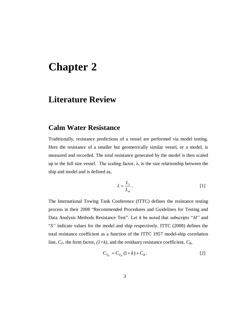
Traditionally, resistance predictions of a vessel are performed via model testing.
Here the resistance of a smaller but geometrically similar vessel, or a model, is
measured and recorded. The total resistance generated by the model is then scaled
up to the full size vessel. The scaling factor, λ, is the size relationship between the
ship and model and is defined as,
m
s
L
L . [1]
The International Towing Tank Conference (ITTC) defines the resistance testing
process in their 2008 “Recommended Procedures and Guidelines for Testing and
Data Analysis Methods Resistance Test”. Let it be noted that subscripts “M” and
“S” indicate values for the model and ship respectively. ITTC (2008) defines the
total resistance coefficient as a function of the ITTC 1957 model-ship correlation
line, CF, the form factor, (1+k), and the residuary resistance coefficient, CR,
RFT CkCCMM
)1( . [2]

4
Here, the total resistance coefficient, CT, is the dimensionless form of the total
resistance, RT,
2
2
1SV
RC
T
T
. [3]
The 1957 ITTC model-ship correlation line is defined as,
2
10 )2)((log
075.0
ReCF . [4]
Here, Re is the Reynolds number given by the expression,
VLRe , [5]
where V is velocity, L is vessel length at the designed waterline, and ν is the
kinematic viscosity of the fluid. The residuary resistance coefficient, CR, from
equation 2, is comprised mostly of wave making resistance. Since corresponding
testing speeds between the model and ship are found using Froude‟s law of
comparison and the Froude number is based on wave patterns, the residuary
resistance coefficient for the model is equal to the residuary resistance coefficient
for the ship. The Froude number is,
gL
VFn , [6]
and Froude‟s law of comparison is,
m
m
s
s
gL
V
gL
V . [7]
The form factor, (1+k), is unique to each vessel based on the ships geometry. The
ITTC (2008) recommended procedure for determining the form factor is to use
Prohaska‟s method of 1966, where CTM/CFM is plotted against Fn4/CFM. It is

5
assumed that in the low speed region, Fn < 0.2, the function Fn4 will be a straight
line and cross the y-axis, when Fn=0, at (1+k). Since testing speeds close to zero
don‟t occur, the tangent must be extended to approximate the form factor.
After the model test is complete, the measured model resistance, RTM, can be scaled
to the ship resistance, RTS, in the following seven steps. Let it be noted that the
correlation allowance, CA, in step 6, accounts for the roughness of the ships surface
that is not present on the model.
1. Nondimensionalize measured RTM values into CTM
2. Calculate CFM (by use of model-ship correlation line)
3. Determine form factor (1+k)
4. CRM=CTM-CFM(1+k)=CRS
5. Calculate CFS
6. CTS=CFS(1+k)+CRS+CA
7. RTS=CTS½ρSV2
Golf Balls
According to John Martin (1968), the first golf ball was sold in 1452 for ten
shillings. As the game developed, so did the balls used to play the game. In 1618
James Melvill of St. Andrews Scotland invented the “featherie", Figure 1.
Figure 1: Featherie (Martin, 1968)

6
This ball was made by stuffing a leather pouch with wet goose down. As the ball
dried the leather shrank and down expanded. This created internal pressure that
rendered a ball that could be hit long distances, bounce, and roll. Unfortunately,
the ball became useless if wet.
By 1846 Rob Patterson invented a new golf ball, the “guttie”. The guttie was
created from gutta percha, a rubber like sap from the Sapodilla tree found in
Malaysia. When the rubber was heated, it could easily be molded into a perfectly
round sphere with a nice, smooth surface. This ball was easily produced, and easily
fixed if damaged. The immediate popularity of the guttie stemmed from its ability
to resist moisture, meaning golfers could now play when it was wet or raining.
However, golfers soon realized that it did not travel as far nor soar through the air
as well as the featherie. Overtime, golfers discovered that the old battered gutties
had better flight characteristics. John Martin (1968) states, “Then it began to be
noticed that scarred-up balls „dooked and shied‟ [ducked and darted] much less
than smooth new ones did. So the gutties were given a few clips with a cleek or
other iron club before being put on sale.”
By 1860, gutties were being manufactured using two part compression molds with
built in “raised ridges” to provide new balls with surface imperfection needed for
better flight, Figure 2.
Figure 2: Guttie with raised ridges (Martin, 1968)

7
It wasn‟t until 1906 that William Taylor developed the modern dimpled golf ball.
With a keen understanding of aerodynamics, Taylor defined a range of criteria that
identifies the geometry of the dimple in order to optimize flight. This concept was
later patented in 1908. Table 1 characterizes the dimple design.
Table 1: Taylor dimple criteria
Ball
Diameter,
mm (in)
Percentage
of Coverage
Dimple Diameter,
mm (in)
[% of ball diameter]
Dimple Depth,
mm (in)
[% of dimple diameter]
41.15 (1.62) 25%-75% 2.29-3.81 (.09-.15)
[5.56%-9.26%]
>0.356 (.014”)
[9.33%-15.56%]
42.67 (1.68) 25%-75% 2.29-3.81 (.09-.15)
[5.36%-8.93%]
>0.356 (.014”)
[9.33%-15.56%]
In the 1930‟s the sport became standardized. In 1931, American golf associations
standardized ball sizes as 42.67mm (1.68 in) in diameter. In 1932, British and
Canadian standard balls sizes became 41.15mm (1.62 in) in diameter. Regardless of
manufacturer, golf balls were now all made with dimples. The average ball
contained 332 to 338 dimples with dimple diameters between 3.18mm (.125 in) and
3.28mm (.129 in) and depths ranging from 0.305 mm (.012 in) to 0.343 mm (.0135
in). Notice these specifications are similar to Taylor‟s dimple criteria, Table 1. The
diameters, 3.18mm (.125 in) to 3.28mm (.129 in), fall exactly between Taylor‟s
optimized dimple diameters, 2.29 mm (.09 in) to 3.81 mm (.15 in). The dimple
depths, 0.305 mm (.012 in) to 0.343 mm (.0135 in), are less than Taylor‟s
recommended minimum dimple depth of 0.356 mm (.014 in); however, the
proportional relationship between dimple depth and dimple diameter is satisfied,
9.33%-15.56%.
John Martin (1968) references a study performed by Dunlop on a 41.15 mm (1.62
in) diameter golf ball. Here the carry, or the distance the ball travels in flight, is

8
compared among balls with several different dimple depths. Results are
summarized in Table 2.
Table 2: Dunlop full-shot test results
Dimple Depth,
mm (in)
Carry,
m (ft)
Carry Plus Roll,
m (ft)
0.025 (.001) 107 (351) 134 (438)
0.102 (.004) 171(561) 194 (636)
0.178 (.007) 194 (636) 212 (696)
0.254 (.010) 204 (669) 218 (714)
0.330 (.013) 218 (714) 239 (783)
0.406 (.016) 206 (675) 219 (720)
To understand why dimpling increases the travel of golf balls, one must understand
a bit of fluid mechanics.
Drag Reduction through Turbulent Boundary
Layers
Laminar Boundary Layers
The fundamental equations of motion for a Newtonian fluid can be express through
Navier-Stokes. According to Kundu (2008) Navier-Stokes may be expressed as
shown in equation 8,
jj
i
i
i
xx
ug
x
p
Dt
Du
2
3 . [8]
An expansion of equation 8 into component form yields,
2
3
1
2
2
2
1
2
2
1
1
2
13
13
2
12
1
11
1 1
x
u
x
u
x
u
x
p
x
uu
x
uu
x
uu
t
u
, [9]

9
2
3
2
2
2
2
2
2
2
1
2
2
23
23
2
22
1
21
2 1
x
u
x
u
x
u
x
p
x
uu
x
uu
x
uu
t
u
, [10]
32
3
3
2
2
2
3
2
2
1
3
2
33
3
3
2
3
2
1
3
1
3 1g
x
u
x
u
x
u
x
p
x
uu
x
uu
x
uu
t
u
. [11]
The nonlinearity of these equations makes them difficult to solve. This is due to
their three dimensional nature and the lack of an explicit solution for pressure;
however, key elements influencing the fluid flow for a certain set of circumstances
can be identified by making assumptions and eliminating non-relevant terms.
Assumptions that allow Navier-Stokes to be reduced include but are not limited to
steady state flow, well developed flow, inviscid flow, two dimensional flow, and
incompressibility. The simplified equations are applicable to circumstances where
the base assumption can be applied.
“In 1905 Ludwig Prandtl…first hypothesized that, for small viscosity, the viscous
forces are negligible everywhere except close to the solid boundaries where the no-
slip condition must be satisfied” (Kundu, 2008). This hypothesis was the first
explanation of the boundary layer, a thin, near wall layer of fluid that satisfied no-
slip and accounted for viscous forces in an otherwise inviscid fluid. The behavior
of the boundary layer is easiest to explain on an infinite flat plate. To determine the
equations of motion within this boundary layer, the following assumptions can be
made,
1. The flow is 2D: u3 and x3 are not considered.
2. The free stream flow is steady: 0
t.
3. The flow is laminar: ν is a molecular property of the fluid.
4. The fluid is incompressible: 02
2
1
1
x
u
x
u.

10
5. Variations across the boundary layer are much faster than variations along
the layer: 21 xx
and
2
2
2
2
1
2
xx
.
6. Reynolds number is large: Rex >> 1.
7. The boundary layer is thin: δ << x.
8. Velocities along the boundary layer are much greater than those across the
boundary layer: u2 << u1.
Applying assumptions 1 though 8 eliminates non-applicable terms from equations
9,10, and 11. For example, equation 9 can be immediately reduced to,
2
2
1
2
2
1
1
2
12
12
1
11
1
x
u
x
u
x
p
x
uu
x
uu
. [12]
Scaling, or non-dimensionalizing the remaining terms with respect to free stream
velocity and geometric length, reduces the equations of motion to the significant
terms based on order of magnitude. According to Kundu (2008) the approximate
equations of motion within the boundary layer in a steady state incompressible
laminar flow are:
2
2
1
2
12
12
1
11
1
x
u
x
p
x
uu
x
uu
, [13]
2
0x
p
, [14]
02
2
1
1
x
u
x
u. [15]
Hill (1992) defines equation 13 as the Momentum Equation. Using the 1921 von
Karman momentum integral method, Hill solves equation 13 in terms of
displacement thickness, δ*, momentum thickness, θ, shear stress at the wall (skin
friction), τ0, and free stream velocity, U. This approximation method finds a
solution that satisfies the integral across the boundary layer but may not satisfy the

11
integral at specific points. It is important because shear stress generated by the
boundary layer can now be approximated in terms of two measurable quantities,
free steam velocity and boundary layer thickness. The solution to equation 13 is the
Karman momentum integral equation,
2
0
1
*
1
2Udx
dU
Udx
d
, [16]
where the skin friction, τ0, is equal to the shear stress at the wall and is expressed as,
2
10
x
u
, [17]
the displacement thickness, δ*, is the thickness of boundary layer that has the effect
of making that thickness unavailable for free stream flow,
2
0
1* 1 dxU
u
, [18]
and the momentum thickness, θ, is the loss of momentum due to the presence of the
boundary layer,
2
0
11 1 dxU
u
U
u
. [19]
Equation 16 is applicable to both laminar and turbulent boundary layers, although
in turbulence the shear stress is not a function of molecular viscosity. Kundu (2008)
states that τ0 must be empirically defined in turbulent boundary layers.
Turbulent Boundary Layers
Considering an infinite flat hydraulically smooth plate, downstream flow becomes
unstable as the local Reynolds number increases, Rex. If the local Reynolds number
exceeds the critical Reynolds number then the flow transitions into turbulence.

12
According to Kundu (2008) the critical Reynolds number is a function of surface
roughness, free stream instabilities, and the shape of the leading edge. For a flat
plate Recr ~ 106.
Under these circumstances, transition to turbulence is not instantaneous. As the
name implies, there exists a region of transition where the laminar flow becomes
unstable before becoming turbulent. Figure 3 demonstrates the transition from
laminar to turbulent flow.
Figure 3: Boundary layer over a flat plate (Pai, 1957)
To estimate the coefficient of friction in the turbulent boundary layer, Pai (1957)
assumes that transition occurs all at one point. Pai (1957) identifies that the
coefficient of friction is higher in a turbulent boundary layer than it is in the
laminar boundary layer for a smooth flat plate. Kundu (2008) agrees that turbulent
boundary layers generate more frictional resistance due to the greater macroscopic
mixing in a turbulent flow.
Transition can be nearly instantaneous if the plate abruptly shifts from
hydraulically smooth. Roughness elements can disturb the laminar flow causing
13
turbulent transition much further upstream. To keep viscous drag low, roughness is
usually avoided.
Separation and the Effects of Turbulence
On a flat plate, turbulent boundary layers increase frictional resistance; but what
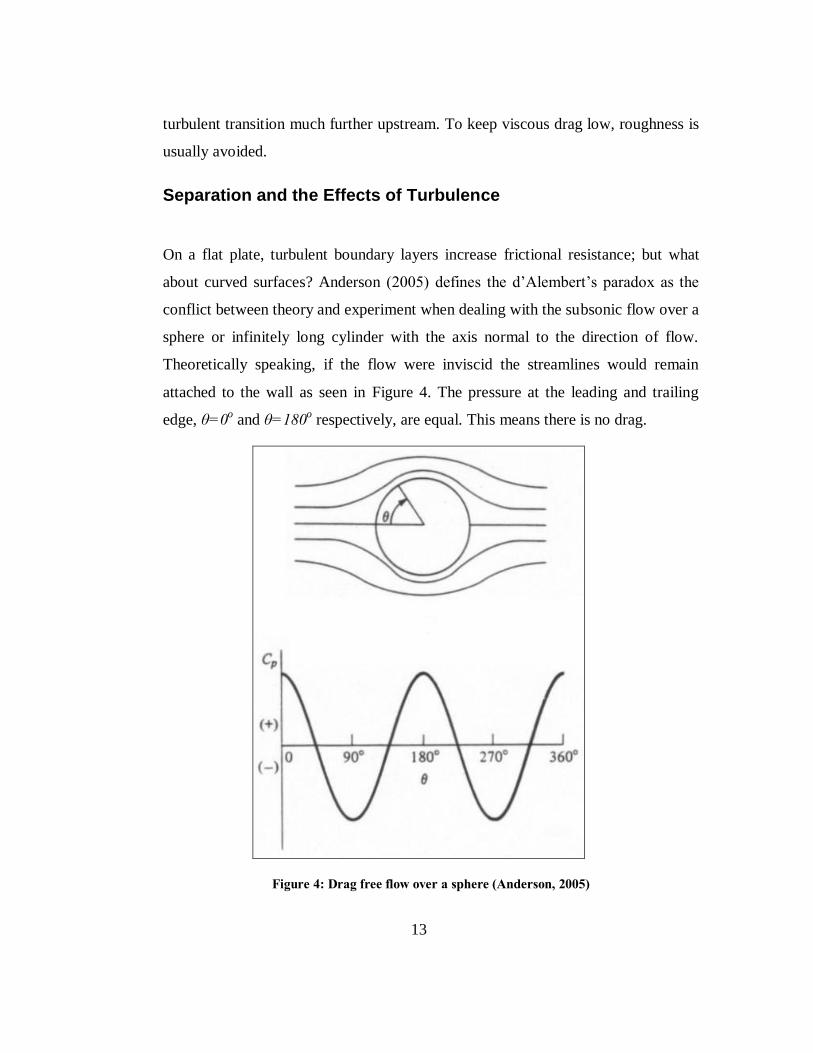
about curved surfaces? Anderson (2005) defines the d‟Alembert‟s paradox as the
conflict between theory and experiment when dealing with the subsonic flow over a
sphere or infinitely long cylinder with the axis normal to the direction of flow.
Theoretically speaking, if the flow were inviscid the streamlines would remain
attached to the wall as seen in Figure 4. The pressure at the leading and trailing
edge, θ=0o and θ=180
o respectively, are equal. This means there is no drag.
Figure 4: Drag free flow over a sphere (Anderson, 2005)
14
Realistically, as the flow diverges about the centerline at the leading edge, the
pressure gradient, δp/δx1, is negative and the flow accelerates around the high side
of the sphere, θ=90o, while the streamlines converge. As the flow progresses
beyond θ=90o to θ=180
o it converges back onto the centerline on the downstream
side of the sphere. Here the streamlines diverge and the flow is forced to slow
down because the pressure gradient, δp/δx1, is positive and “pushes back” against
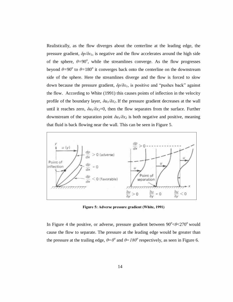
the flow. According to White (1991) this causes points of inflection in the velocity
profile of the boundary layer, δu1/δx2. If the pressure gradient decreases at the wall
until it reaches zero, δu1/δx2=0, then the flow separates from the surface. Further
downstream of the separation point δu1/δx2 is both negative and positive, meaning
that fluid is back flowing near the wall. This can be seen in Figure 5.
Figure 5: Adverse pressure gradient (White, 1991)
In Figure 4 the positive, or adverse, pressure gradient between 90o<θ<270
o would
cause the flow to separate. The pressure at the leading edge would be greater than
the pressure at the trailing edge, θ=0o and θ=180
o respectively, as seen in Figure 6.

15
Figure 6: Real flow over a sphere (Anderson, 2005)
This pressure gradient is known as pressure drag or form drag. For objects of
curvature, the total resistance is a function of frictional resistance and form drag.
Kundu (2008) states the flow around a sphere with a Reynolds number less than
3x10⁵ has a laminar boundary layer. This flow would separate at θ=82
o. If the
Reynolds number is increased beyond 3x10⁵ the boundary layer becomes turbulent
and separation occurs at θ=125o. In other words, a turbulent boundary layer has the
ability to delay flow separation. Because of the sphere‟s geometry, this would
reduce the size of the downstream turbulent wake. In two dimensional terms, the
area of separation is reduced. If the flow separates further downstream then the

16
pressure gradient from leading to trailing edge is smaller and form drag is reduced.
Hill (1992) explains why a turbulent boundary layer delays separation,
…transition behavior takes place in the boundary layer, resulting in
a significant reduction in its tendency to separate. The reason for
this is that the turbulent fluctuations constitute a mechanism for
transporting high momentum from the outer part of the layer to the
region near the wall. The effect is as if there were an increased shear
stress or…an increased coefficient of viscosity. This tends to raise
the wall shear stress, but it also means that the turbulent boundary
fluid can climb higher up the pressure hill than the fluid in the
laminar layer…the fact that the turbulent layer tends to have much
higher momentum (and shear stress) near the wall gives it an
increased resistance to separation.
If the boundary layer is naturally laminar, turbulence can be forced to achieve
separation delay. As mentioned earlier, alterations from a hydraulically smooth
surface can cause instabilities and turbulence. This surface roughness can take the
form of convexities or concavities. Figure 7 represents the effects of dimples on
boundary layer transition and separation specifically in the case of a golf ball.

17
Figure 7: Airflow comparison of smooth ball vs. golf ball (Scott, 2005)
Figure 7 demonstrates how dimples are used to induce turbulent boundary layers.
How can we be certain the dimples, or concavities, will create a turbulent boundary
layer? According to Seebass (1990),
On the other hand, when the surface is concave, the fluid element
moved to a greater radius is confined to a lower velocity region
where the local radial pressure gradient is too low to force it back to
a lower radius. The fluid element thus continues to move radially

18
outward until it meets the surface. This mechanism makes the flow
over a concave surface inherently unstable.
In other words, flow over a concave surface is likely to become turbulent. On a
small scale, dimples are concave surfaces.
Since a single dimple is relatively small compared to the surface area of the sphere,
about 0.1%, the effects of a dimple can be estimated as a roughness element;
therefore, a pattern of dimples can be estimated as surface roughness. The effect of
roughness on transition is highly influenced by element shape, size, and spacing.
Recognizing the work performed by Prandtl and Schlichting in 1934, Pai (1957)
acknowledges that no surface is perfectly smooth. For this reason, a permissible
amount of roughness should be determined so that smooth surface boundary layer
approximations can be used in spite of the roughness. To determine the admissible
roughness, hsa, the following equation can be used.
100
saUh. [20]
This equation assumes the surface is covered with uniform sand roughness where
hsa is the maximum allowable grain size before the roughness effects turbulent
transition. The effects of a roughness element on turbulent transition can be seen in
Figure 8.
Figure 8: Boundary layer transition and the effects of roughness (Pai, 1957)

19
Here, transition occurs more abruptly and further upstream compared to a
hydraulically smooth plate. According to Dryden (1953), as the height of the
roughness element, h, increases, the transition point, xt, approaches the position of
the roughness element, xh. For engineering purposes, if the dimple dimensions are
greater than the admissible roughness in equation 20, the dimples will influence
turbulent transition. Designed correctly, dimples can almost instantly transition
laminar boundary layers to turbulent boundary layers. This increases viscous
resistance but delays separation, therefore reducing pressure drag. Given the correct
circumstances dimples can be used to reduce the total drag on an object.

20
Chapter 3
Hypothesis
It is understood that dimples are placed on a golf ball to trip the boundary layer
from laminar to turbulent in order to delay flow separation. This decreases the
pressure gradient from leading to trailing edge and therefore decreases pressure
drag. It is believed that the same concept can be adapted for use on a ship to
decrease total resistance. This hypothesis is based on some fundamental
assumptions:
1. The geometry of the vessel allows for flow separation.
2. The boundary layer of the vessel is laminar, may contain instabilities, but is
not turbulent.
In order for the geometry of the vessel to accommodate flow separation the aft
portions of the vessel must taper back towards the centerline. This would allow for
the creation of the adverse pressure gradient that causes separation. If separation
occurs then pressure drag is a contributor to the total resistance. Here the concept of
separation control can be applied.
The vessel must also operate at relatively lower speeds to ensure the boundary layer
is naturally laminar. Dimpling the hull, as done with a golf ball, will trip the
boundary layer from laminar to turbulent, delay flow separation further
21
downstream, and decrease drag. If the boundary layer is naturally turbulent, then
dimpling will have no affect on the mean flow.

22
Chapter 4
Vessel Parameters
Compared to a sphere or an infinite cylinder, a ship is relatively slender. For this
reason, vessel selection plays a key role in testing this hypothesis. Planing hulls
were eliminated as an option for this study for a number of reasons, primarily
because the geometry of most planning vessels does not allow for flow separation.
Very commonly, planning vessels have square transoms where the waterlines do
not taper back towards the centerline. This is not conducive for separation delay.
The fluid separates from the hull because the hull no longer exists downstream. In a
sense, separation delay is like reattaching the flow to the object surface. If the
object does not exist downstream, then the flow cannot be reattached.
Eliminating planning hulls also eliminated the complexity of the air/sea surface
interface and narrowed the field of selection to displacement hulls. The geometry of
a displacement hull remains submerged below the surface. This means the hull is
exposed to one fluid. This is a simpler approach for a proof of concept.
Additionally, displacement hulls commonly have waterlines with tapered aft
portions and operate at relatively lower speeds. Displacement hulls are a far better
hull form to test this hypothesis.

23
Vessel parameters for the vessel used in this study, at the tested displacements, are
show in Table 3. Vessel displacements and wetted surface areas are shown in Table
4 and Table 5.
Table 3: Vessel parameters
4.3 m (14 ft) Waterline 5.2 m (17 ft) Waterline
Ship,
m (ft)
Model,
m (ft)
Ship,
m (ft)
Model,
m (ft)
LWL 59.8 (196.3) 2.05 (6.73) LWL 60.8 (199.5) 2.09 (6.85)
Breadth 9.9 (32.4) 0.34 (1.11) Breadth 9.9 (32.5) 0.34 (1.12)
Draft 4.3 (14) 0.15 (0.48) Draft 5.2 (17) 0.18 (0.58)
CB 0.626 0.626 CB 0.602 0.602
Table 4: Table of displacements and wetted areas (ship)
Vessel
T,
m (ft) ,
m3 (ft
3)
Δ,
tonnes (lb)
S,
m2 (ft
2)
1.83 (6) 488 (17243) 502 (1107023) 453 (4876)
2.44 (8) 723( 25530) 743 (1639023) 531 (5717)
3.05 (10) 974 (34408) 1002 (2209019) 608 (6546)
3.66 (12) 1239 (43772) 1275 (2810159) 686 (7384)
4.27 (14) 1516 (53551) 1559 (3437981) 764 (8224)
4.88 (16) 1804 (63704) 1855 (4089812) 842 (9065)
5.18 (17) 1951 (68894) 2006 (4422995) 881 (9487)
Table 5: Table of displacements and wetted areas (model)
Model
T,
m (ft) ,
m3 (ft
3)
Δ,
tonnes (lb)
S,
m2 (ft
2)
0.063 (0.206) 0.020 (0.697) 0.020 (43.472) 0.533 (5.742)
0.084 (0.275) 0.029 (1.031) 0.029 (64.363) 0.625 (6.731)
0.105 (0.343) 0.039 (1.390) 0.039 (86.747) 0.716 (7.708)
0.126 (0.412) 0.050 (1.768) 0.050 (110.353) 0.808 (8.694)
0.146 (0.480) 0.061 (2.164) 0.061 (135.007) 0.900 (9.684)
0.167 (0.549) 0.073 (2.574) 0.073 (160.604) 0.922 (10.673)
0.178 (0.583) 0.079 (2.783) 0.079 (173.688) 1.038 (11.170)

24
Surface data for the ship was reversed engineering using the table of offset in Table
6. Ordinates in are spaced 6.1 m (20 ft) apart. The lines plan can be seen in Figure 9
and Figure 10
Table 6: Table of offsets (ship)
Ordinate
Waterline
0.61 m
(2 ft)
1.22 m
(4 ft)
1.83 m
(6 ft)
3.66 m
(12 ft)
5.49 m
(18 ft)
A n/a n/a n/a 0.20
(0.67)
2.04
(6.70)
0 n/a n/a n/a 1.12
(3.69)
2.66
(8.71)
0.5 0.20
(0.67)
0.31
(1.01)
0.41
(1.34)
2.45
(8.04)
3.78
(12.40)
1 0.71
(2.35)
1.12
(3.69)
1.74
(5.70)
3.47
(11.39)
4.29
(14.07)
1.5 1.43
(4.69)
2.04
(6.70)
2.66
(8.71)
4.09
(13.40)
4.29
(14.74)
2 2.35
(7.71)
3.06
(10.05)
3.57
(11.73)
4.45
(14.61)
4.70
(15.41)
3 4.09
(13.40)
4.49
(14.74)
4.70
(15.41)
4.80
(15.75)
4.90
(16.08)
4 4.60
(15.08)
4.90
(16.08)
4.90
(16.08)
4.90
(16.08)
5.00
(16.42)
5 4.70
(15.41)
5.00
(16.42)
5.00
(16.42)
5.00
(16.42)
5.00
(16.42)
6 4.60
(15.08)
4.90
(16.08)
4.90
(16.08)
5.00
(16.42)
4.90
(16.08)
7 3.98
(13.07)
4.39
(14.41)
4.56
(14.94)
4.80
(15.75)
4.90
(16.08)
8 2.70
(8.85)
3.27
(10.72)
3.47
(11.39)
4.09
(13.40)
4.49
(14.74)
8.5 1.84
(6.03)
2.35
(7.71)
2.66
(8.71)
3.27
(10.72)
3.88
(12.73)
9 1.02
(3.35)
1.43
(4.69)
1.63
(5.36)
2.14
(7.04)
3.06
(10.05)
9.5 0.25
(0.80)
0.47
(1.54)
0.61
(2.01)
1.02
(3.35)
1.84
(6.03)
10 n/a n/a n/a n/a 0.41
(1.34)

25
Figure 9: Plan and profile view

26
Figure 10: Body plan view

27
To create the model, the 3D data was scaled using a scaling factor of 29.14. The
table of offsets for the model is shown in Table 7.
Table 7: Table of offsets (model)
Ordinate
Waterline
20.83 mm
(0.82 in)
41.91 mm
(1.65 in)
62.74 mm
(2.47 in)
125.48 mm
(4.94 in)
188.21 mm
(7.41 in)
A n/a n/a n/a 7.01
(0.28)
70.09
(2.76)
0 n/a n/a n/a 38.55
(1.52)
91.12
(3.59)
0.5 7.01
(0.28)
10.51
(0.41)
14.02
(0.55)
84.11
(3.31)
129.67
(5.11)
1 24.53
(0.97)
38.55
(1.52)
59.58
(2.35)
119.16
(4.69)
147.19
(5.80)
1.5 49.06
(1.93)
70.09
(2.76)
91.12
(3.59)
140.18
(5.52)
154.20
(6.07)
2 80.61
(3.17)
105.14
(4.14)
122.66
(4.83)
152.80
(6.02)
161.21
(6.35)
3 140.18
(5.52)
154.20
(6.07)
161.21
(6.35)
164.72
(6.48)
168.22
(6.62)
4 157.71
(6.21)
168.22
(6.62)
168.22
(6.62)
168.22
(6.62)
171.73
(6.76)
5 161.21
(6.35)
171.73
(6.76)
171.73
(6.76)
171.73
(6.76)
171.73
(6.76)
6 157.71
(6.21)
168.22
(6.62)
168.22
(6.62)
171.73
(6.76)
168.22
(6.62)
7 136.68
(5.38)
150.70
(5.93)
156.31
(6.15)
164.72
(6.48)
168.22
(6.62)
8 92.52
(3.64)
112.15
(4.42)
119.16
(4.69)
140.18
(5.52)
154.20
(6.07)
8.5 63.08
(2.48)
80.61
(3.17)
91.12
(3.59)
112.15
(4.42)
133.18
(5.24)
9 35.05
(1.38)
49.06
(1.93)
56.07
(2.21)
73.60
(2.90)
105.14
(4.14)
9.5 8.41
(0.33)
16.12
(0.63)
21.03
(0.83)
35.05
(1.38)
63.08
(2.48)
10 n/a n/a n/a n/a 14.02
(0.55)
28
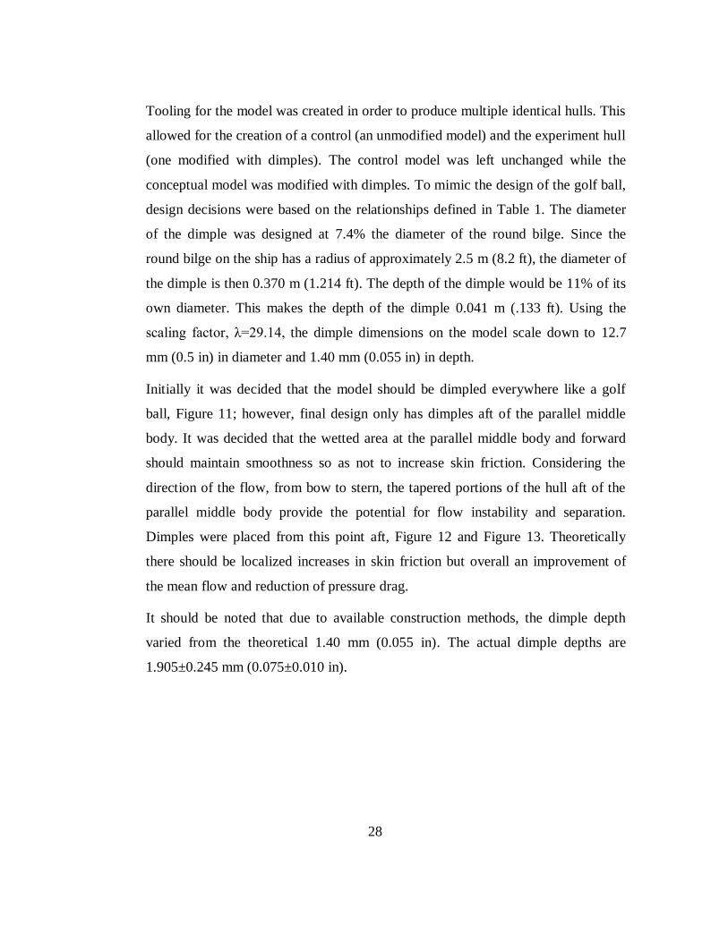
Tooling for the model was created in order to produce multiple identical hulls. This
allowed for the creation of a control (an unmodified model) and the experiment hull
(one modified with dimples). The control model was left unchanged while the
conceptual model was modified with dimples. To mimic the design of the golf ball,
design decisions were based on the relationships defined in Table 1. The diameter
of the dimple was designed at 7.4% the diameter of the round bilge. Since the
round bilge on the ship has a radius of approximately 2.5 m (8.2 ft), the diameter of
the dimple is then 0.370 m (1.214 ft). The depth of the dimple would be 11% of its
own diameter. This makes the depth of the dimple 0.041 m (.133 ft). Using the
scaling factor, λ=29.14, the dimple dimensions on the model scale down to 12.7
mm (0.5 in) in diameter and 1.40 mm (0.055 in) in depth.
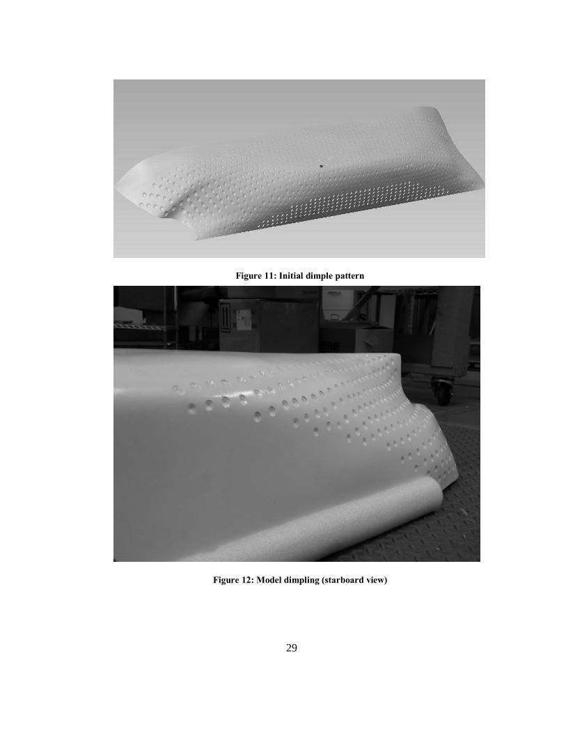
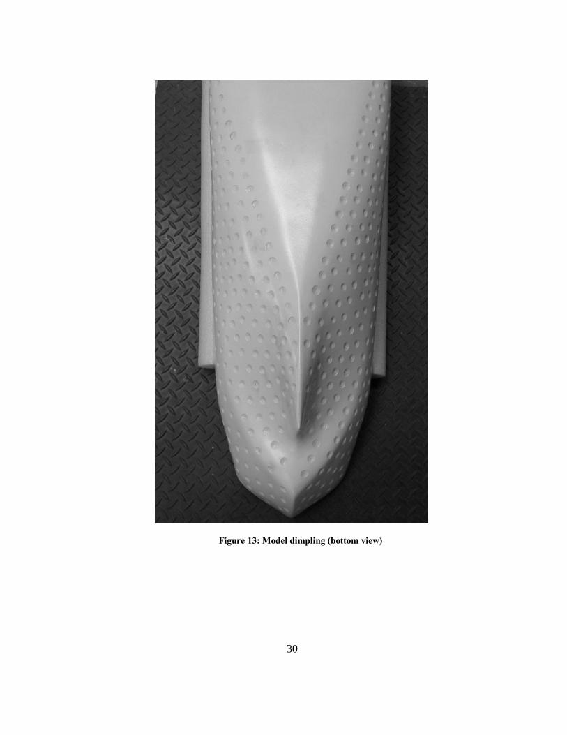
Initially it was decided that the model should be dimpled everywhere like a golf
ball, Figure 11; however, final design only has dimples aft of the parallel middle
body. It was decided that the wetted area at the parallel middle body and forward
should maintain smoothness so as not to increase skin friction. Considering the
direction of the flow, from bow to stern, the tapered portions of the hull aft of the
parallel middle body provide the potential for flow instability and separation.
Dimples were placed from this point aft, Figure 12 and Figure 13. Theoretically
there should be localized increases in skin friction but overall an improvement of
the mean flow and reduction of pressure drag.
It should be noted that due to available construction methods, the dimple depth
varied from the theoretical 1.40 mm (0.055 in). The actual dimple depths are
1.905±0.245 mm (0.075±0.010 in).
29
Figure 11: Initial dimple pattern
Figure 12: Model dimpling (starboard view)
30
Figure 13: Model dimpling (bottom view)

31
Chapter 5
Results
Resistance tests were performed at the University of Michigan‟s Marine
Hydrodynamic Laboratory. All tests conformed to the ITTC Testing and Data
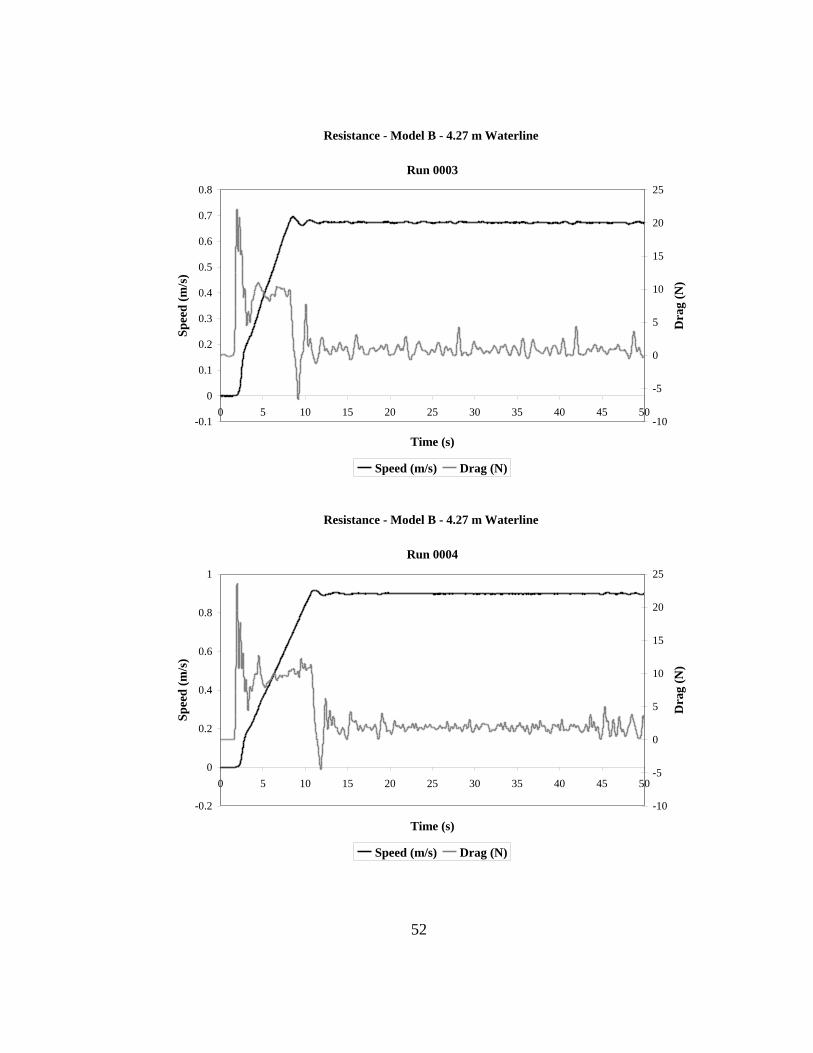
Analysis Methods Resistance Test (2008). Let it be noted that model “A” refers to
the control, or unmodified model, and model “B” refers to the concept, or dimpled
model.
Both models were tested at two displacements, 61.53 kg (135.65 lb) and 78.78 kg
(173.69 lb). These displacements represent the fourteen and seventeen foot
waterlines on the full size vessels. Table 8 and Table 9 are the comparative results
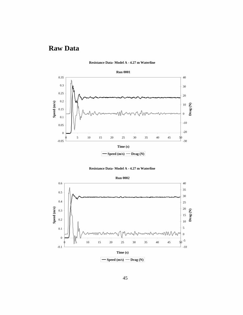
of the resistance tests performed on the models. The values in Table 8 and Table 9
are the average resistance of the models while the carriage traveled at a constant
speed. This neglects erroneous forces generated during acceleration and
deceleration. Raw data for each run can be seen in the Appendix.

32
Table 8: Resistance comparison 4.27 m (14 ft) waterline
Fn RTM A
N (lb)
RTM B
N (lb) % difference
0.10 0.451 (0.101) 0.314 (0.071) -30.39%
0.15 1.083 (0.243) 0.887 (0.199) -18.11%
0.20 2.090 (0.470) 1.869 (0.420) -10.58%
0.25 3.579 (0.804) 3.236 (0.727) -9.59%
0.30 7.850 (1.764) 8.127 (1.826) 3.53%
0.35 12.268 (2.757) 12.770 (2.870) 4.09%
0.39 18.520 (4.162) 19.382 (4.356) 4.66%
0.40 19.986 (4.492) 21.191 (4.762) 6.03%
Table 9: Resistance comparison 5.18 m (17 ft) waterline
Fn RTM A
N (lb)
RTM B
N (lb) % difference
0.10 0.523 (0.118) 0.568 (0.128) 8.61%
0.15 1.247 (0.280) 1.271 (0.286) 1.95%
0.20 2.329 (0.523) 2.429 (0.546) 4.27%
0.25 4.188 (0.941) 4.231 (0.951) 1.03%
0.30 9.577 (2.152) 9.602 (2.158) 0.26%
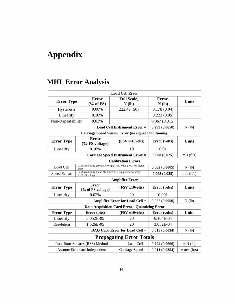
Experimental error in the load cell is ± 0.294 N (0.066 lb). An error analysis for the
Marine Hydrodynamic Laboratories was provided by the University of Michigan
and is reported in the Appendix. Unfortunately, nearly all the results in Table 8 and
Table 9 have overlapping error between model A and model B. If the results
between model A and model B have overlapping error then the percent difference
is not valid. The only results that did not have overlapping error were Fn=0.39 and
Fn=0.40 in Table 8. This can be seen in Figure 14 and Figure 15.

33
Resistance Comparison - 4.27 m Waterline
-5.0
0.0
5.0
10.0
15.0
20.0
25.0
0.2 0.4 0.6 0.8 1.0 1.2 1.4 1.6 1.8
Carriage Speed (m/s)
Res
ista
nce
(N
)
Model A Model B
Figure 14: Resistance comparison – 4.27 m (14 ft) waterline
Resistance Comparison - 5.18 m Waterline
0.0
2.0
4.0
6.0
8.0
10.0
12.0
0.4 0.5 0.6 0.7 0.8 0.9 1.0 1.1 1.2 1.3 1.4
Carriage Speed (m/s)
Res
ista
nce
(N
)
Model A Model B
Figure 15: Resistance comparison – 5.18 m (17 ft) waterline

34
The model resistance was then extrapolated into the resistance of the full size
vessel. The correlation allowance, CA, for the Marine Hydrodynamic Laboratories
is 2.5x10⁻⁴
. Full size resistance data can be seen in Table 10, Table 11, Figure 16
and Figure 17.
Table 10: Extrapolated resistance data – 4.27 m (14 ft) waterline
Fn RTS A
N (lb)
RTS B
N (lb) % difference
0.10 5.24E+03
(1.18E+03)
3.82E+03
(8.59E+02) -27.08%
0.15 1.51E+04
(3.39E+03)
1.43E+04
(3.20E+03) -5.39%
0.20 3.28E+04
(7.36E+03)
3.40E+04
(7.64E+03) 3.84%
0.25 6.12 E+04
(1.37E+04)
6.26E+04
(1.41E+04) 2.27%
0.30 1.59E+05
(3.56E+04)
1.79E+05
(4.03E+04) 13.23%
0.35 2.59E+05
(5.81E+04)
2.90E+05
(6.51E+04) 11.92%
0.39 4.06E+05
(9.12E+04)
4.50E+05
(1.01E+05) 10.87%
0.40 4.41E+05
(9.90E+04)
4.94E+05
(1.11E+05) 12.17%
Table 11: Extrapolated resistance data – 5.18 m (17 ft) waterline
Fn RTS A
N (lb)
RTS B
N (lb) % difference
0.10 6.09E+03
(1.37E+03)
6.83E+03
(1.53E+03) 12.07%
0.15 1.73E+04
(3.89E+03)
1.70E+04
(3.83E+03) -1.60%
0.20 3.57E+04
(8.01E+03)
3.67E+04
(8.25E+03) 2.92%
0.25 7.20E+04
(1.62E+04)
7.09E+04
(1.59E+04) -1.52%
0.30 1.96E+05
(4.40E+04)
1.94E+05
(4.35E+04) -1.16%

35
CTS vs Fn
4.27 m Waterline
0.00E+00
2.00E-03
4.00E-03
6.00E-03
8.00E-03
1.00E-02
1.20E-02
1.40E-02
1.60E-02
0.10 0.15 0.20 0.25 0.30 0.35 0.40
Fn
CT
S
Model A Model B
Figure 16: CTS vs. Fn – 4.27 m (14 ft) waterline
CTS vs. Fn
5.18 m Waterline
0.00E+00
1.00E-03
2.00E-03
3.00E-03
4.00E-03
5.00E-03
6.00E-03
7.00E-03
8.00E-03
9.00E-03
0.10 0.12 0.14 0.16 0.18 0.20 0.22 0.24 0.26 0.28 0.30
Fn
CT
S
Model A Model B
Figure 17: CTS vs. Fn – 5.18 m (17 ft) waterline
36
Chapter 6
Discussion
The lack of difference between model A and model B is easily identifiable. Table 8
and Table 9 show that all results but two are non-valid results. Based on the size of
the measurements taken and the magnitude of error, stochastically speaking, the
recorded resistance values of each model could potentially be equal. In other words,
there was effectively no difference in the resistance characteristics of model B
compared to model A.
There are a number of reasons that could explain why the resistance of model B did
not improve. One thought is that the dimples were incorrectly located, meaning
they were placed too far forward or too far aft. If they were placed too far forward,
assuming separation delay occurred, then there was an even balance between
increased skin friction and decreased pressure drag. Remember that separation
delay is like “reattaching” the flow. Since the flow is in contact with the surface
longer, skin friction increases. In addition, dimpling the hull increases wetted
surface area and makes the flow turbulent, also increasing viscous resistance. If the
relation between increased skin friction and decreased pressure drag is 1:1, than the
resistance characteristics of model B would be unchanged compared to model A.
By placing dimples too for forward the mean flow is exposed to more dimples than

37
necessary, the flow is turbulent longer than necessary, and skin friction is increased
as much as pressure drag is decreased.
If the dimples were placed too far aft, assuming separation occurred, than the
dimples had no effect on the boundary layer. In other words, the flow separated
from the hull before reaching the dimples. This is like not having dimples there at
all. Under these circumstances the results of model B would be like testing model
A twice. The lack of difference between the results would only prove the
repeatability of the tooling that the models were created from.
The dimples could also have been designed incorrectly. Assuming the dimples
were located correctly and exposed to laminar flow, than the dimple diameter and
dimple depth did not create turbulence and separation delay did not occur. Without
separation delay, pressure drag remains unchanged. Here the dimples may be too
small and/or too shallow.
Improper dimple design could also contribute to increased skin friction. Assuming
the mean flow was not “over-exposed” to dimples; an improperly designed dimple
could potentially create turbulence and delay separation, but increase skin friction
such that in cancels out the decrease in pressure drag. Here, the dimples may too
large and/or too deep.
Another explanation for the lack of differences may be vessel selection, meaning
separation naturally does not occur on this particular vessel. Here the tapered
portions of the stern do not curve fast enough to create an adverse pressure gradient
and separation does not occur. Pressure drag is now negligible and therefore cannot
be improved upon; however, this is a weak explanation because the presence of
dimples in a flow that did not separate should have logically increased skin friction.
This effect would have been reflected in the results.
Lastly, experimental error could have contributed to the experiments results.
Sources of error in this experiment include but are not limited to yaw, sway,

38
location of tow points, and the size of the models. Yaw is the rotational movement
of a vessel about the z or x3 axis. Figure 18 demonstrates vessel motions. If the
vessel yaws during the resistance test, resistance would drastically increase. To
prevent yaw, the University of Michigan‟s Marine Hydrodynamic Laboratory
(MHL) uses a “grass hopper.” This is a device that restrains the model from yawing
while maintaining freedom of motion in heave and pitch. For this particular
experiment, the vessel size did not accommodate the use of the grass hopper. The
models were too small for the grass hopper to reach the bow. Instead, the clamps
that hold the heave staff in place were tightened such that the frictional force of the
clamps would restrain the model in yaw. To ensure proper alignment of the model,
before each run the centerline of the model was aligned with the centerline of the
carriage using a pendulum. To verify that the model had not yawed during the run,
after each run the alignment was checked using a pendulum. The thoroughness of
the procedure is such that yaw most likely did not contribute to experimental error;
nevertheless, since the grass hopper was not used, it may exist and therefore needed
to be discussed.
Figure 18: Vessel motions (Newman, 1978)

39
According to Timothy Peters, the assistant director at the MHL, the rails of the
carriage are similar to a roller coaster. The wheels of the carriage roll on both the
top and the sides of the rails so that it can travel along the rail yet not fall off. Due
to tolerance stack ups, the carriage is capable of yawing from port to starboard up
to ± 1 inch during a run. Systematic errors like this one affect the results of every
run. The error is consistent and therefore even if the error was significant the results
are usable for comparison studies. According to Timothy Peters, experimental error
at the MHL is minimal and results can be considered accurate.
The tow points of model A and model B were installed at slightly different
locations. Both tow points were installed along the centerline; both were 0.098 m
(0.323 ft) above the baseline; however, the tow point of Model A was 1.099 m
(3.604 ft) aft of the forward perpendicular while the tow point of model B was
1.032 m (3.385 ft) aft of the forward perpendicular. Different tow point locations
means different moments were generated on the models during forward motion.
Potentially, the models would squat and pitch differently during their runs, altering
the comparative results between model A and model B.
Indisputably, the largest source of error came from the size of the models. A seven
foot model is not large enough to test properly at the MHL. As discussed, the
models were too small to use with the grass hopper. More importantly, a smaller
model means smaller resistance measurements. Smaller resistance measurements
mean that experimental error in the measurement equipment becomes a significant
portion of the measurement itself. For the 4.27 m (14 ft) waterline, experimental
error in the load cell was 2.75% to 187% of the measurements and averaged
35.51%. It was not until Fn exceeded 0.35 that error became 3% or less of the
measurements being taken. At the 4.27 m (14 ft) waterline, only two valid
differences were measured at Fn=0.39 and Fn=0.4. At the 5.18 m (17 ft) waterline
40
error ranged from 6% to 112% of the measurements and averaged 40%. With error
being such a large potion of the measurement, results between model A and model
B would need to vary greatly for differences to be valid. As seen in Table 8 and
Table 9, that is not so.
.
41
Chapter 7
Conclusions
Based on these results, it cannot be determined if the reduction of ship resistance
through induced turbulent boundary layers was a success for this hull form;
however, it can be concluded that it was not a failure. The hypothesis was neither
proved nor disproved providing motivation for further investigation. If this topic is
to be reinvestigated, it is the suggestion of the author that a more systematic
approach be taken.
The primary reason for the lack of valid experimental evidence is the small size of
the models. Before retesting this hypothesis, larger models should be created. This
would increase the magnitude of the resistance values making experimental error a
smaller portion of the value measured. Here smaller percent differences between
baseline and concept models would be considered valid. Increasing model size to
12 foot would triple the resistance values measured by the load cell. For future
research, model size should be increased to a minimum of 3.66 m (12 ft).
Before reinvestigating this topic, flat plate testing should be performed to better
understand the effects of dimples. A flat plate in the presence of an adverse
pressure gradient would act as the baseline. By modifying the size, depth, and
pattern of the dimples on the plate, it could be better understood how different

42
dimples affect separation with respect to different pressure gradients. The
information from these experiments would allow for educated decisions when it
comes time to modify one of the model boats.
When a vessel is selected a wake survey should be performed on the control model
to verify that the hull form is a candidate for separation delay. A wake survey
would demonstrate that separation naturally occurs on the selected vessel and
estimate the proportion of total drag due to form drag. This would act as a phase
gate in the experimental process. Either the selected vessel would meet the
separation criteria and move to the next step or it will reveal the hull to be
unworthy of study and a new vessel can be selected.
Once a ship passes the wake survey, flow visualization should be used to determine
separation points. Determining separations points allows for the proper location of
dimples based on information gathered from flat plate testing. Flow visualization
can be accomplished experimentally or be numerically simulated. This ensures the
dimples are not placed too far forward or too far aft, optimizing the relationship
between increased skin friction and decreased pressure drag.
The adverse pressure gradients that are causing separation should also be measured.
The measured pressure gradients on the model can be correlated to the adverse
pressure gradients in the flat plate testing. The size, depth, and pattern of the
dimples can be designed from the information in the flat plate study that optimized
separation delay.
Resistance tests on both models would then be compared as done in this thesis. In
addition, after dimpling, the wake survey and flow visualization should be repeated
on the concept model. By repeating the tests, it can be established that separation
delay did or did not occur. Knowledge of this information would aid greatly when
making conclusions.

43
References
Anderson, John D. (2005): “Introduction to Flight” McGraw Hill, Ed. 5, pp 348-
352
Dryden, Hugh L. (1953): “Review of Published Data on the Effect of Roughness on
Transition from Laminar to Turbulent Flow”, Journal of Aeronautical Science,
V. 20, No. 7, July 1953, pp 477-482
Hill, Philip G. and Peterson, Carl R. (1992): “Mechanics and Thermodynamics of
Propulsion” Addison-Wesley Publishing Company Inc., Ed. 2, pp 93-124
International Towing Tank Conference (2008): “Testing and Data Analysis
Methods Resistance Test” ITTC Recommended Procedure and Guidelines, Rev.
2, pp 1-13
Kundu, Pijush K. and Cohen, Ira M. (2008): “Fluid Mechanics” Elsevier Inc., Ed. 4,
pp 104-105, 340-400
Martin, John Stuart (1968): “The Curious History of the Golf Ball, Mankind‟s Most
Fascinating Sphere” Horizon Press, NY, pp 25-129
Newman, J. N. (1978): “Theory of Ship Motions”, Advances in Applied Mechanics,
Massachusetts Institute of Technology, Cambridge Massachusetts, Vol. 18, pp
221-283
Pai, Shih-I (1957): “Viscous Flow Theory, II – Turbulent Flow”, D. Van Nostrand
Company, Inc., pp 60-114
Scott, J. (2005): "Golf Ball Dimples and Drag," Aerospaceweb.org, 10 July 2010,
<http://www.aerospaceweb.org/question/aerodynamics/q0215.shtml>
Seebass, Richard A. (1990): “Viscous Drag Reduction in Boundary Layers”
Progress in Astronautics and Aeronautics, V. 123, pp 3-320
White, Frank M. (1991): “Viscous Fluid Flow”, McGraw-Hill, Inc., Ed. 2. pp 218-
495
44
Appendix
MHL Error Analysis
Load Cell Error
Error Type Error
(% of FS)
Full Scale,
N (lb)
Error,
N (lb) Units
Hysteresis 0.08% 222.49 (50) 0.178 (0.04)
Linearity 0.10% 0.223 (0.05)
Non-Repeatability 0.03% 0.067 (0.015)
Load Cell Instrument Error = 0.293 (0.0658) N (lb)
Carriage Speed Sensor Error (no signal conditioning)
Error Type Error
(% FS voltage) (FSV 0-10volts) Error (volts) Units
Linearity 0.10% 10 0.01
Carriage Speed Instrument Error = 0.008 (0.025) m/s (ft/s)
Calibration Errors
Load Cell Calibrated using precision weights verifiedon precision digital
scale 0.002 (0.0005) N (lb)
Speed Sensor Calibrated using Fluke Multimeter w/ Frequency accuracy
0.1% FS voltage 0.008 (0.025) m/s (ft/s)
Amplifier Error
Error Type Error
(% of FS voltage) (FSV ±10volts) Error (volts) Units
Linearity 0.02% 20 0.001
Amplifier Error for Load Cell = 0.022 (0.0050) N (lb)
Data Acquisition Card Error - Quantizing Error
Error Type Error (bits) (FSV ±10volts) Error (volts) Units
Linearity 3.052E-05 20 6.104E-04
Resolution 1.526E-05 20 3.052E-04
DAQ Card Error for Load Cell = 0.015 (0.0034) N (lb)
Propagating Error Totals
Root-Sum-Squares (RSS) Method Load Cell = 0.294 (0.0660) ± N (lb)
Assume Errors are Independent Carriage Speed = 0.011 (0.0354) ± m/s (ft/s)
45
Raw Data
Resistance Data- Model A - 4.27 m Waterline
-0.05
0
0.05
0.1
0.15
0.2
0.25
0.3
0.35
0 5 10 15 20 25 30 35 40 45 50
Time (s)
Sp
eed
(m
/s)
-30
-20
-10
0
10
20
30
40
Run 0001
Dra
g (
N)
Speed (m/s) Drag (N)
Resistance Data- Model A - 4.27 m Waterline
-0.1
0
0.1
0.2
0.3
0.4
0.5
0.6
0 5 10 15 20 25 30 35 40 45 50
Time (s)
Sp
eed
(m
/s)
-10
-5
0
5
10
15
20
25
30
35
40
Run 0002
Dra
g (
N)
Speed (m/s) Drag (N)

46
Resistance Data- Model A - 4.27 m Waterline
-0.1
0
0.1
0.2
0.3
0.4
0.5
0.6
0.7
0.8
0 5 10 15 20 25 30 35 40 45 50
Time (s)
Sp
eed
(m
/s)
-20
-10
0
10
20
30
40
50
Run 0003
Dra
g (
N)
Speed (m/s) Drag (N)
Resistance Data- Model A - 4.27 m Waterline
-0.2
0
0.2
0.4
0.6
0.8
1
0 5 10 15 20 25 30 35 40 45 50
Time (s)
Sp
eed
(m
/s)
-10
0
10
20
30
40
50
Run 0004
Dra
g (
N)
Speed (m/s) Drag (N)

47
Resistance Data- Model A - 4.27 m Waterline
-0.2
0
0.2
0.4
0.6
0.8
1
1.2
1.4
0 5 10 15 20 25 30 35 40 45 50
Time (s)
Sp
eed
(m
/s)
-50
-40
-30
-20
-10
0
10
20
30
40
50
Run 0005
Dra
g (
N)
Speed (m/s) Drag (N)
Resistance Data- Model A - 4.27 m Waterline
-0.2
0
0.2
0.4
0.6
0.8
1
1.2
1.4
1.6
0 5 10 15 20 25 30 35 40 45 50
Time (s)
Sp
eed
(m
/s)
-50
-40
-30
-20
-10
0
10
20
30
40
50
Run 0006
Dra
g (
N)
Speed (m/s) Drag (N)

48
Resistance Data- Model A - 4.27 m Waterline
-0.2
0
0.2
0.4
0.6
0.8
1
1.2
1.4
1.6
0 5 10 15 20 25 30 35 40 45 50
Time (s)
Sp
eed
(m
/s)
-5
0
5
10
15
20
25
30
35
40
45
Run 0007
Dra
g (
N)
Speed (m/s) Drag (N)
Resistance Data- Model A - 4.27 m Waterline
-0.2
0
0.2
0.4
0.6
0.8
1
1.2
1.4
1.6
1.8
0 5 10 15 20 25 30 35 40 45 50
Time (s)
Sp
eed
(m
/s)
-5
0
5
10
15
20
25
30
35
40
45
Run 0008
Dra
g (
N)
Speed (m/s) Drag (N)

49
Resistance Data- Model A - 4.27 m Waterline
-0.2
0
0.2
0.4
0.6
0.8
1
1.2
1.4
1.6
1.8
0 5 10 15 20 25 30 35 40 45 50
Time (s)
Sp
eed
(m
/s)
-5
0
5
10
15
20
25
30
35
40
45
Run 0009
Dra
g (
N)
Speed (m/s) Drag (N)
Resistance Data- Model A - 4.27 m Waterline
-0.2
0
0.2
0.4
0.6
0.8
1
1.2
1.4
1.6
1.8
2
0 5 10 15 20 25 30 35 40 45 50
Time (s)
Sp
eed
(m
/s)
-40
-30
-20
-10
0
10
20
30
40
50
Run 0010
Dra
g (
N)
Speed (m/s) Drag (N)

50
Resistance Data- Model A - 4.27 m Waterline
-0.5
0
0.5
1
1.5
2
0 5 10 15 20 25 30 35 40 45 50
Time (s)
Sp
eed
(m
/s)
-30
-20
-10
0
10
20
30
40
50
Run 0011
Dra
g (
N)
Speed (m/s) Drag (N)
Resistance Data- Model A - 4.27 m Waterline
-0.5
0
0.5
1
1.5
2
0 5 10 15 20 25 30 35 40 45 50
Time (s)
Sp
eed
(m
/s)
-30
-20
-10
0
10
20
30
40
50
Run 0012
Dra
g (
N)
Speed (m/s) Drag (N)

51
Resistance - Model B - 4.27 m Waterline
-0.05
0
0.05
0.1
0.15
0.2
0.25
0.3
0 5 10 15 20 25 30 35 40 45 50
Time (s)
Sp
eed
(m
/s)
-8
-6
-4
-2
0
2
4
6
8
10
12
14
Run 0001
Dra
g (
N)
Speed (m/s) Drag (N)
Resistance - Model B - 4.27 m Waterline
-0.1
0
0.1
0.2
0.3
0.4
0.5
0 5 10 15 20 25 30 35 40 45 50
Time (s)
Sp
eed
(m
/s)
-10
-5
0
5
10
15
20
25
Run 0002
Dra
g (
N)
Speed (m/s) Drag (N)
52
Resistance - Model B - 4.27 m Waterline
-0.1
0
0.1
0.2
0.3
0.4
0.5
0.6
0.7
0.8
0 5 10 15 20 25 30 35 40 45 50
Time (s)
Sp
eed
(m
/s)
-10
-5
0
5
10
15
20
25
Run 0003
Dra
g (
N)
Speed (m/s) Drag (N)
Resistance - Model B - 4.27 m Waterline
-0.2
0
0.2
0.4
0.6
0.8
1
0 5 10 15 20 25 30 35 40 45 50
Time (s)
Sp
eed
(m
/s)
-10
-5
0
5
10
15
20
25
Run 0004
Dra
g (
N)
Speed (m/s) Drag (N)

53
Resistance - Model B - 4.27 m Waterline
-0.2
0
0.2
0.4
0.6
0.8
1
1.2
1.4
0 5 10 15 20 25 30 35 40 45 50
Time (s)
Sp
eed
(m
/s)
-5
0
5
10
15
20
25
Run 0005
Dra
g (
N)
Speed (m/s) Drag (N)
Resistance - Model B - 4.27 m Waterline
-0.2
0
0.2
0.4
0.6
0.8
1
1.2
1.4
1.6
0 5 10 15 20 25 30 35 40 45 50
Time (s)
Sp
eed
(m
/s)
-5
0
5
10
15
20
25
Run 0006
Dra
g (
N)
Speed (m/s) Drag (N)

54
Resistance - Model B - 4.27 m Waterline
-0.2
0
0.2
0.4
0.6
0.8
1
1.2
1.4
1.6
1.8
0 5 10 15 20 25 30 35 40 45 50
Time (s)
Sp
eed
(m
/s)
-5
0
5
10
15
20
25
Run 0007
Dra
g (
N)
Speed (m/s) Drag (N)
Resistance - Model B - 4.27 m Waterline
-0.2
0
0.2
0.4
0.6
0.8
1
1.2
1.4
1.6
1.8
0 5 10 15 20 25 30 35 40 45 50
Time (s)
Sp
eed
(m
/s)
-5
0
5
10
15
20
25
Run 0008
Dra
g (
N)
Speed (m/s) Drag (N)
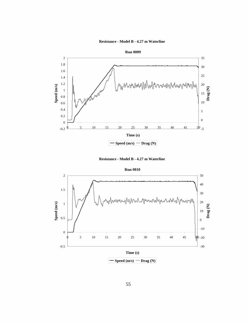
55
Resistance - Model B - 4.27 m Waterline
-0.2
0
0.2
0.4
0.6
0.8
1
1.2
1.4
1.6
1.8
2
0 5 10 15 20 25 30 35 40 45 50
Time (s)
Sp
eed
(m
/s)
-5
0
5
10
15
20
25
30
35
Run 0009
Dra
g (
N)
Speed (m/s) Drag (N)
Resistance - Model B - 4.27 m Waterline
-0.5
0
0.5
1
1.5
2
0 5 10 15 20 25 30 35 40 45 50
Time (s)
Sp
eed
(m
/s)
-30
-20
-10
0
10
20
30
40
50
Run 0010
Dra
g (
N)
Speed (m/s) Drag (N)

56
Resistance - Model B - 4.27 m Waterline
-0.5
0
0.5
1
1.5
2
0 5 10 15 20 25 30 35 40 45 50
Time (s)
Sp
eed
(m
/s)
-30
-20
-10
0
10
20
30
40
50
Run 0011
Dra
g (
N)
Speed (m/s) Drag (N)
Resistance - Model A - 5.18 m Waterline
-0.1
0
0.1
0.2
0.3
0.4
0.5
0.6
0 5 10 15 20 25 30 35 40 45 50
Time (s)
Sp
eed
(m
/s)
-20
-10
0
10
20
30
40
50
60
Run 0001
Dra
g (
N)
Speed (m/s) Drag (N)
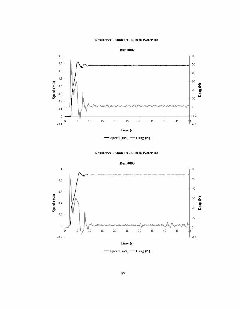
57
Resistance - Model A - 5.18 m Waterline
-0.1
0
0.1
0.2
0.3
0.4
0.5
0.6
0.7
0.8
0 5 10 15 20 25 30 35 40 45 50
Time (s)
Sp
eed
(m
/s)
-20
-10
0
10
20
30
40
50
60
Run 0002
Dra
g (
N)
Speed (m/s) Drag (N)
Resistance - Model A - 5.18 m Waterline
-0.2
0
0.2
0.4
0.6
0.8
1
0 5 10 15 20 25 30 35 40 45 50
Time (s)
Sp
eed
(m
/s)
-10
0
10
20
30
40
50
60
Run 0003
Dra
g (
N)
Speed (m/s) Drag (N)

58
Resistance - Model A - 5.18 m Waterline
-0.2
0
0.2
0.4
0.6
0.8
1
1.2
1.4
0 5 10 15 20 25 30 35 40 45 50
Time (s)
Sp
eed
(m
/s)
-20
-10
0
10
20
30
40
50
60
Run 0004
Dra
g (
N)
Speed (m/s) Drag (N)
Resistance - Model A - 5.18 m Waterline
-0.2
0
0.2
0.4
0.6
0.8
1
1.2
1.4
1.6
0 5 10 15 20 25 30 35 40 45 50
Time (s)
Sp
eed
(m
/s)
-10
0
10
20
30
40
50
Run 0005
Dra
g (
N)
Speed (m/s) Drag (N)

59
Resistance - Model B - 5.18 m Waterline
-0.1
0
0.1
0.2
0.3
0.4
0.5
0.6
0 5 10 15 20 25 30 35 40 45 50
Time (s)
Sp
eed
(m
/s)
-20
-10
0
10
20
30
40
50
60
Run 0001
Dra
g (
N)
Speed (m/s) Drag (N)
Resistance - Model B - 5.18 m Waterline
-0.1
0
0.1
0.2
0.3
0.4
0.5
0.6
0.7
0.8
0 5 10 15 20 25 30 35 40 45 50
Time (s)
Sp
eed
(m
/s)
-20
-10
0
10
20
30
40
50
60
Run 0002
Dra
g (
N)
Speed (m/s) Drag (N)
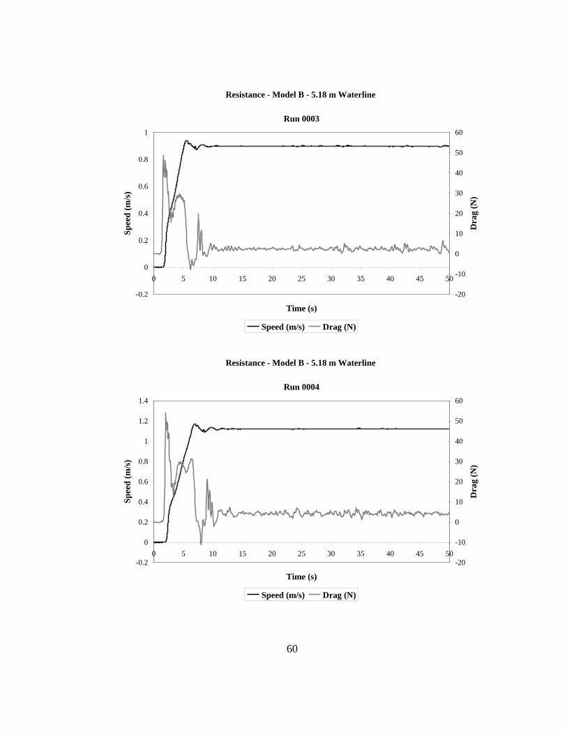
60
Resistance - Model B - 5.18 m Waterline
-0.2
0
0.2
0.4
0.6
0.8
1
0 5 10 15 20 25 30 35 40 45 50
Time (s)
Sp
eed
(m
/s)
-20
-10
0
10
20
30
40
50
60
Run 0003
Dra
g (
N)
Speed (m/s) Drag (N)
Resistance - Model B - 5.18 m Waterline
-0.2
0
0.2
0.4
0.6
0.8
1
1.2
1.4
0 5 10 15 20 25 30 35 40 45 50
Time (s)
Sp
eed
(m
/s)
-20
-10
0
10
20
30
40
50
60
Run 0004
Dra
g (
N)
Speed (m/s) Drag (N)

61
Resistance - Model B - 5.18 m Waterline
-0.2
0
0.2
0.4
0.6
0.8
1
1.2
1.4
1.6
0 5 10 15 20 25 30 35 40 45 50
Time (s)
Sp
eed
(m
/s)
-10
0
10
20
30
40
50
60
Run 0005
Dra
g (
N)
Speed (m/s) Drag (N)

62
Sample Calculations
Table 12: Model-ship correlation calculations
Model A – 5.18 m (17 ft) Waterline
V carriage,
m/s (ft/s)
RTMA,
N (lb) Fn CTM Re M CFM
0.448 (1.471) 0.523 (0.118) 0.10 5.017E-03 8.64E+05 4.840E-03
0.673 (2.207) 1.247 (0.280) 0.15 5.316E-03 1.30E+06 4.434E-03
0.897 (2.944) 2.329 (0.523) 0.20 5.577E-03 1.73E+06 4.176E-03
1.120 (3.675) 4.188 (0.941) 0.25 6.437E-03 2.16E+06 3.992E-03
1.347 (4.420) 9.577 (2.152) 0.30 1.018E-02 2.60E+06 3.849E-03
Model B – 5.18 m (17 f)t Waterline
V carriage,
m/s (ft/s)
RTMB,
N (lb) Fn CTM Re M CFM
0.477 (1.468) 0.568 (0.128) 0.10 5.470E-03 8.63E+05 4.842E-03
0.673 (2.208) 1.271 (0.286) 0.15 5.410E-03 1.30E+06 4.433E-03
0.898 (2.948) 2.429 (0.546) 0.20 5.803E-03 1.73E+06 4.175E-03
1.121 (3.679) 4.231 (0.951) 0.25 6.488E-03 2.16E+06 3.991E-03
1.347 (4.419) 9.602 (2.158) 0.30 1.021E-02 2.60E+06 3.849E-03
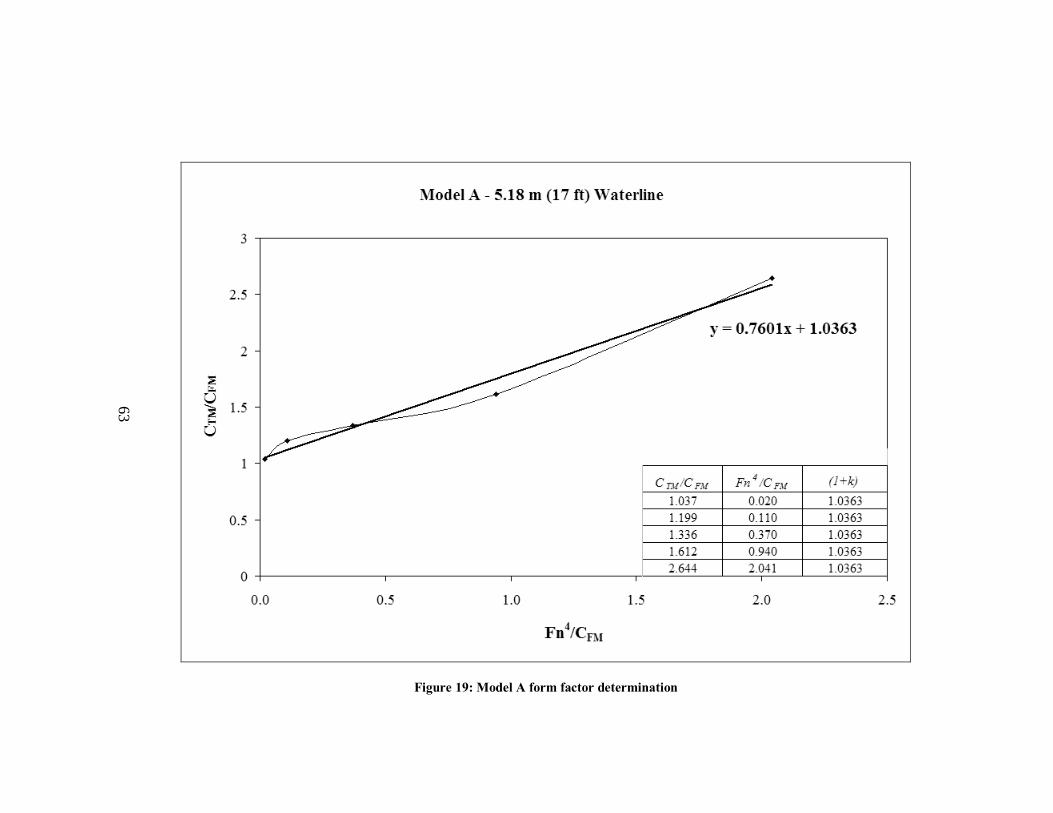
63
Figure 19: Model A form factor determination
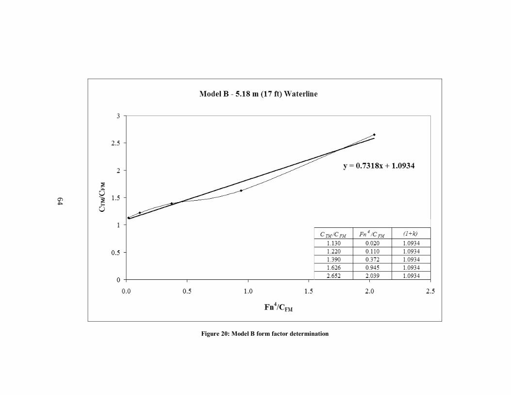
64
Figure 20: Model B form factor determination
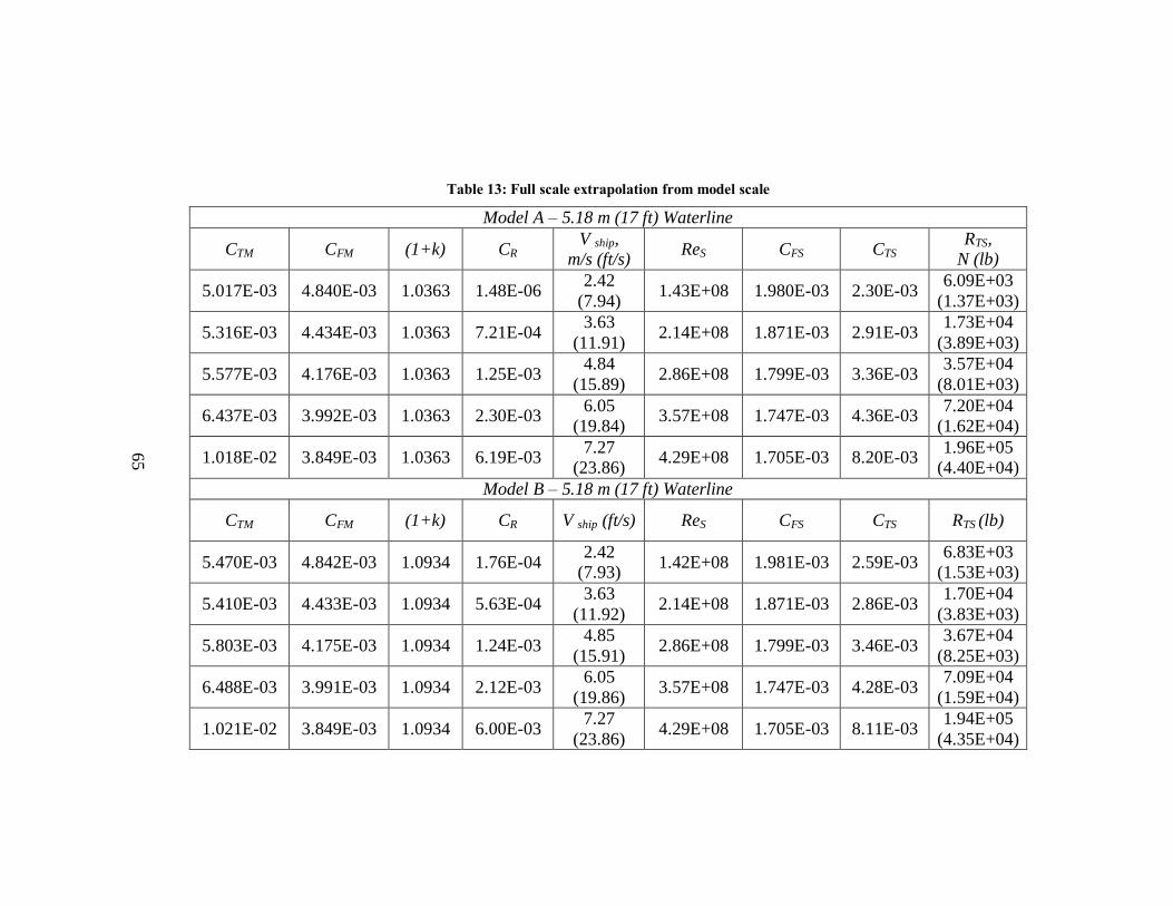
65
Table 13: Full scale extrapolation from model scale
Model A – 5.18 m (17 ft) Waterline
CTM CFM (1+k) CR V ship,
m/s (ft/s) ReS CFS CTS
RTS,
N (lb)
5.017E-03 4.840E-03 1.0363 1.48E-06 2.42
(7.94) 1.43E+08 1.980E-03 2.30E-03
6.09E+03
(1.37E+03)
5.316E-03 4.434E-03 1.0363 7.21E-04 3.63
(11.91) 2.14E+08 1.871E-03 2.91E-03
1.73E+04
(3.89E+03)
5.577E-03 4.176E-03 1.0363 1.25E-03 4.84
(15.89) 2.86E+08 1.799E-03 3.36E-03
3.57E+04
(8.01E+03)
6.437E-03 3.992E-03 1.0363 2.30E-03 6.05
(19.84) 3.57E+08 1.747E-03 4.36E-03
7.20E+04
(1.62E+04)
1.018E-02 3.849E-03 1.0363 6.19E-03 7.27
(23.86) 4.29E+08 1.705E-03 8.20E-03
1.96E+05
(4.40E+04)
Model B – 5.18 m (17 ft) Waterline
CTM CFM (1+k) CR V ship (ft/s) ReS CFS CTS RTS (lb)
5.470E-03 4.842E-03 1.0934 1.76E-04 2.42
(7.93) 1.42E+08 1.981E-03 2.59E-03
6.83E+03
(1.53E+03)
5.410E-03 4.433E-03 1.0934 5.63E-04 3.63
(11.92) 2.14E+08 1.871E-03 2.86E-03
1.70E+04
(3.83E+03)
5.803E-03 4.175E-03 1.0934 1.24E-03 4.85
(15.91) 2.86E+08 1.799E-03 3.46E-03
3.67E+04
(8.25E+03)
6.488E-03 3.991E-03 1.0934 2.12E-03 6.05
(19.86) 3.57E+08 1.747E-03 4.28E-03
7.09E+04
(1.59E+04)
1.021E-02 3.849E-03 1.0934 6.00E-03 7.27
(23.86) 4.29E+08 1.705E-03 8.11E-03
1.94E+05
(4.35E+04)