Reducing Petroleum Consumption from Transportation

Christopher R. Knittel

December 2011 CEEPR WP 2011-020

A Joint Center of the Department of Economics, MIT Energy Initiative and MIT Sloan School of Management.

Reducing Petroleum Consumption from Transportation

Christopher R. Knittel∗

December 30, 2011

Abstract

The United States consumed more petroleum-based liquid fuel per capita than any other OECD-

high-income country—30 percent more than the second-highest country (Canada) and 40 per-

cent more than the third-highest (Luxemburg). This paper examines the main channels through

which reductions in U.S. oil consumption might take place: (a) increased fuel economy of ex-

isting vehicles, (b) increased use of non-petroleum-based low-carbon fuels, (c) alternatives to

the internal combustion engine, and (d) reduced vehicles miles travelled. I then discuss how

the policies for reducing petroleum consumption used in the US compare with the standard

economics prescription for using a Pigouvian tax to deal with externalities. Taking into account

that energy taxes are a political hot button in the United States, and also considering some

evidence that consumers may not correctly value fuel economy, I offer some thoughts about the

margins on which policy aimed at reducing petroleum consumption might usefully proceed.

∗I benefited from discussions with Hunt Allcott, Severin Borenstein, Joseph Doyle, Stephen Holland, JonathanHughes, Kenneth Gillingham, Donald MacKenzie, Joan Ogden, and Victor Stango. William Barton Rogers Professorof Energy Economics, Sloan School of Management, Massachusetts Institute of Technology and National Bureau ofEconomic Research. Email: knittel@mit.edu.

1 Introduction

The United States consumed more petroleum-based liquid fuel per capita than any other OECD-

high-income country—30 percent more than the second-highest country (Canada) and 40 percent

more than the third-highest (Luxemburg). The transportation sector accounts for 70 percent of

U.S. oil consumption and 30 percent of U.S. greenhouse gas emissions. Gasoline and diesel fuels,

alone, account for 60 percent of oil consumption. The economic argument for seeking to reduce this

level of consumption of petroleum-based liquid fuel begins with the externalities associated with

high levels of U.S. consumption of petroleum-based fuels.

First, burning petroleum contributes to local pollution. The transportation sector accounts for

67 percent of carbon monoxide emissions, 45 percent of nitrogen oxide (NOx) emissions, and 8

percent of particulate matter emissions. These pollutants lead to health problems ranging from

respiratory problems to cardiac arrest. Furthermore, automobiles emit both NOx and volatile

organic compounds which, combined with heat and sunlight, form ground-level ozone, or smog.

Currie and Walker (2011) and Knittel, Miller, and Sanders (2011) both find that decreases in

traffic reduce infant mortality.

Second, burning a gallon of gasoline causes roughly 25 pounds of carbon dioxide to be emitted

into the atmosphere, which raises the risks of destructive climate change. Greenstone, Kopits, and

Wolverton (2011) estimate the social cost of carbon under a variety of assumptions. They estimate

an SSC as high as $65 per metric ton of carbon dioxide (and gases with an effect equivalent to

carbon dioxide) in 2010, but values that are often in the range of $21 to $35 per metric ton. Tol

(2008) is a meta-study of the existing literature, for studies written after 2001, he finds the median

social cost of carbon ranges from $17 to $62 per metric ton of CO2-equivalent.

The U.S. dependence on imported gasoline has had other costs, too, including the military

expense of trying to assure stability in oil-producing regions (for example, ICTA (2005)), and the

relationship between oil price shocks and macroeconomic downturns. These, too, can be viewed

as negative externalities. But this paper neither focuses on these various externalities and social

costs, nor delves into the literature about quantifying them. Instead, I take their existence as

largely given, and instead focus on understanding the policy tools that seek to reduce gasoline

consumption.

Of course, an obvious starting point for economists is to look at prices: although the price of

petroleum is set in a global market, government taxes on petroleum vary quite substantially. Table

1 lists taxes on gasoline and diesel on a per gallon basis as of 2010 for OECD Category I countries—

essentially the worlds most developed economies. The United States and Canada are clearly outliers,

1

with taxes on gasoline below $1 per gallon. How do these price differences affect consumption?

Figure 1 is suggestive. It plots the per capita petroleum-based liquid fuel consumption for these

countries versus the gasoline price in that country, with the size of the bubbles are proportional

to population. The regression line is population-weighted, but looks similar if it is not weighted.

It would require quite a bit of additional argument and delicacy to estimate a reliable elasticity of

demand from this data, but for the record, the slope of fitted log-log regression line through these

data is -1.86. If one were to also include the log of income as an explanatory variable in such a

regression, the coefficient associated with the log of gasoline prices is -1.49, while the coefficient

associated with the log of income is 1.05.

The relative fuel use across the United States and other OECD Category I countries is, at

least in part, a by-product of differences in the types and use of light-duty vehicles. Schipper

(2006) reports that the average gallons-per-mile of European fleets in 2005 was below 0.034 (29.4

miles-per-gallon), while the average gallons-per-mile of the U.S. fleet was 0.051 (19.6 miles-per-

gallon). Because of differences in how fuel efficiency is evaluated, this finding probably understates

the European advantage. Similarly, Schipper reports that per capita miles travelled in European

countries is between 35 to 45 percent of U.S. miles travelled.

The next four sections of this paper examine the main channels through which reductions in

U.S. oil consumption might take place: (a) increased fuel economy of existing vehicles, (b) increased

use of non-petroleum-based low-carbon fuels, (c) alternatives to the internal combustion engine,

and (d) reduced vehicles miles travelled. I then discuss how these policies for reducing petroleum

consumption compare with the standard economics prescription for using a Pigouvian tax to deal

with externalities. Taking into account that energy taxes are a political hot button in the United

States, and also considering some evidence that consumers may not correctly value fuel economy, I

offer some thoughts about the margins on which policy aimed at reducing petroleum consumption

might usefully proceed.

2 Improved Fuel Economy

Shortly after the oil prices shocks of the 1970s, the United States adopted Corporate Average

Fuel Economy (CAFE) standards, which set minimum average fuel economy thresholds for the

new vehicles sold by an automaker in a given year. Figure 2 shows how the standard evolved. For

passenger cars, the standard increased by only 0.5 miles-per-gallon from 1984 to 2010; for light-duty

trucks, the increase was only 3.5 miles-per-gallon over this same time period. From 1978 to 1991 the

2

standard for light trucks differentiated between two- and four-wheel drive trucks, but manufacturers

could also choose to meet a combined-truck standard. By world standards, these miles-per-gallon

standards are not aggressive. After accounting for differences in the testing procedures, the World

Bank estimated that the European Union standard was roughly 17 miles-per-gallon more stringent

in 2010 than the U.S. standard (An, Earley, and Green-Weiskel (2011)).

Manufacturers who violate the CAFE standard pay a fine of roughly $50 per mile-per-gallon

per vehicle for violating the standard. Historically, U.S. manufacturers have complied with the

standard. Asian manufacturers have typically exceeded the standard in each year, while European

manufacturers have typically violated the standard and paid the fines. Trading between man-

ufacturers was not allowed, so there was no possibility for certain manufacturers to accumulate

credits for selling a higher proportion of fuel-efficient cars and then selling those credits to other

manufacturers.

Other than the fact that the standards have barely budged over the last three decades, two

features of the original CAFE standards reduced their effect. First, sport-utility vehicles were

treated as light trucks, and thus could meet a lower miles-per-gallon standard than cars. Perhaps

not coincidentally, in 1979 light trucks comprised less than 10 percent of the new vehicle fleet, but

this share rose steadily and peaked in 2004 at 60 percent. Second, vehicles with a gross vehicle

weight of over 8,500 pounds, which includes many large pickup trucks and sports-utility vehicles,

were exempt from CAFE standards.

Actual new vehicle fleet fuel economy in the United States has changed little since the early

1980s. Figure 3 plots the fuel economy of passenger vehicles (cars) and light duty trucks from 1979

to 2011. The figure shows that while the average fuel economy of both cars and trucks increased

over this time period, fleet fuel economy fell as consumers shifted away from cars and into trucks.

The figure also shows that during the run-up in gasoline prices beginning in 2005, fleet fuel economy

increased. This rise appears to have subsided by 2010.

Although the fuel economy of new U.S. vehicles gradually declined through the 1980s and 1990s,

there was scope for substantial improvements. In the short run, when the set of offered vehicles is

fixed, car-buyers could choose vehicles with higher fuel efficiency. In 2011, for example, while the

mean passenger car available for sale was rated at 23 miles-per-gallon, 10 percent of passenger cars

had a rating of 30 miles-per-gallon or above. The highest rating for 2011 was the Nissan Leaf at

99 miles-per-gallon; the Toyota Prius had a combined fuel economy rating of 50 miles-per-gallon.

In the medium run, automakers can adjust vehicle attributes by trading off weight and horse-

power for increased fuel economy. Knittel (2011) finds that reducing weight by 1 percent increases

3

fuel by roughly 0.4 percent, while reducing horsepower and torque by 1 percent increases fuel

economy by roughly 0.3 percent

In the long run, manufacturers can push out the frontier. Knittel (2011) estimates that had

manufactures put all of the technological progress observed in the market from 1980 to 2006 into fuel

economy, instead of putting it into attributes that increased horsepower and/or weight, average fuel

economy would have increased by 60 percent, instead of the 11.6 percent increase actually observed.

On average, a vehicle with a given weight and engine power level has a fuel economy that is 1.75

percent higher than a vehicle with the same weight and horsepower level from in the previous

year. While the analysis in Knittel (2011) ends in 2006, using similar data and empirical models

through model year 2011, the technological frontier has shifted out at an average rate of 1.97 and

1.51 percent per year from 2006 to 2011 for passenger cars and light-duty trucks, respectively,

suggesting that no technological barrier has yet been reached. The greater availability of hybrids

and plug-in hybrids also suggest that progress is likely to continue.

Gasoline prices do seem to affect choices about which cars to buy. A number of papers have

used this variation in gasoline prices to estimate the magnitude of this response. These papers

inevitably estimate a short run response to gasoline prices—in the particular sense that the choice

set of vehicles is usually held fixed. Busse, Knittel, and Zettelmeyer (2009) estimate that over the

period of 1999 to 2008, the market share of vehicles in the bottom quartile of fuel efficiency, among

those vehicles offered in a given year, falls by nearly 24 percent for every $1 increase in gasoline

prices. In contrast, the market share of the upper quartile of vehicles as ranked by fuel efficiency

increases by over 20 percent. They also show that the market share of compact cars increases by 24

percent for every $1 increase in gasoline prices, while the market share of sport-utility vehicles falls

by 14 percent. Klier and Linn (forthcoming) estimate a logit demand system and focus on the effects

of changes in a vehicles cost-per-mile on demand. They find that a 5-cent increase in a vehicles

cost per mile, equivalent to a one-dollar increase in gasoline prices for a 20 miles-per-gallon vehicle,

decreases the log of its market share by between 0.5 and 0.8, all else equal.1 In the aggregate, this

translates to an increase in average fuel economy of between 0.5 and 1.2 miles-per-gallon for every

$1 dollar increase in gas prices. Again, their estimates hold the set of offered vehicles fixed. Li,

Timmins, and von Haefen (2009) find similar effects.

A new Corporate Average Fuel Economy standard in place for 2011 seeks to increase average

fuel economy to roughly 34.1 miles-per-gallon by 2016. The Environmental Protection Agency

1These coefficients represent the change in a vehicles log of market share when the vehicles cost per mile increases.Of course, if this is driven from changes in gasoline prices, then the cost of all vehicles cost per mile will change. Thisexplains why these effects are so large.

4

and Department of Transportation are currently in the rulemaking process for model years 2017

and beyond, with President Obama and 13 automakers agreeing to a standard of 54.5 miles-per-

gallon by 2025. A number of notable changes have occurred. First, the mileage standards are now

based to some extent on the greenhouse gas emissions of the vehicle, which can deviate from fuel

economy because of ancillary greenhouse gas emissions associated with, for example, air conditioner

refrigerant leaks. Second, the new standards are footprint-based, in which each vehicle face a

standard based on the area of the footprint of its tires; larger footprints face a lower standard.

For example, the 2011 Honda Civic coupe has a footprint of 43 square feet, while the 2011 Ford

F-150 SuperCab has a footprint of 67 square feet. In 2016, these vehicles would face fuel efficiency

standards of 41.1 miles-per-gallon and 24.7 miles-per-gallon, respectively.2 For more details on the

fuel efficiency rules for the next few years, see U.S. Energy Information Administration (2007) and

U.S. Environmental Protection Agency (2010).

Is new vehicle fuel economy of 34.1 and 54.5 miles-per-gallon in 2016 and 2025, respectively,

attainable? If we take the average rates of technological progress from Knittel (2011) and a new

vehicle fuel economy in 2010 of roughly 29 miles-per-gallon, new vehicle fuel economy in 2016 would

be roughly 32 miles-per-gallon in 2016, close to the standard of 34.1 miles-per-gallon. Using the

estimated trade-off coefficients, getting to 34.1 miles-per-gallon would require reducing weight and

engine power by less than 6 percent. Alternatively, increasing the rate of technological progress to

2.75 percent per year would achieve the mark.

And, what about the 2025 standard of 54.5 miles-per-gallon in 2025. Taken literally, it would

require fundamental changes to rates of technological progress and/or the size and power of vehicles.

The 2025 number is a bit misleading. In the law, the 54.5 miles-per-gallon standard is based on a

calculation from the Environmental Protection Agency based on carbon dioxide tailpipe emissions.

It also includes credits for many technologies, including plug-in hybrids, electric and hydrogen

vehicles, improved air conditioning efficiency; and others. On an apples-to-apples basis, Roland

(2011) cites some industry followers that claim that the actual new fleet fuel economy in 2025 is

more like to 40 miles-per-gallon. Achieving 40 miles-per-gallon by 2025 is certainly possible. At

a rate of technological progress of 1.75 percent per year, 40 miles-per-gallon requires additional

reductions in weight and engine power of less than 7 percent.

2See, http://www.nhtsa.gov/cars/rules/cafe/overview.htm. The sticker fuel economy is roughly 80 percent of howthe vehicle is counted for the CAFE standard.

5

3 Alternative Fuels

Biofuels are derived from biological components like corn, soybeans, sugar, grasses, and wood chips.

The ethanol produced by this process is an imperfect substitute for gasoline, although bio-diesel as

a nearly perfect substitute for petroleum-based diesel. (Methanol is another alcohol and imperfect

substitute for gasoline that can be derived from either methane—that is, natural gas—or coal.)

Biofuels also hold the potential to have lower carbon emissions. If the plant material could be

grown and converted to liquid fuel using only technologies that do not produce any greenhouse gas

emissions and not lead to land use changes that increase greenhouse gases, then biofuels would not

emit any net greenhouse gases over the life-cycle.

In practice, the lifecycle emissions of biofuels are affected by a number of factors. First, the

feedstock used affects carbon emissions during the growing stage—for example, through fertiliza-

tion. The most common feedstock used in the U.S. is corn. Brazilian ethanol is made from sugar

cane. So-called second generation or cellulosic ethanol uses feedstocks that require little in the way

of irrigation and fertilizer during the growing process, such as miscanthus and switchgrass. Second,

the fuel used for generation of heat and electricity during refining process affects emissions. Third,

the calculation is affected by whether the co-products from distilling, notably distillery grains with

solubles, are dried before being sold and whether these emissions should be included, or treated as

another product.

Fourth, the life-cycle emissions of corn-based biofuels are affected by the milling process. Corn

ethanol is typically refined using either a dry or wet milling process. Under wet milling, the corn

is soaked in hot water and sulfurous acid. The starches from this mixture are then separated and

fermented, leading to ethanol. Dry milling requires less energy and generates fewer greenhouse gas

emissions, but does not yield as many co-products as wet milling. Under dry milling, the corn

is ground into flour and cooked along with enzymes, where yeast is added for fermentation. The

ethanol is then separated from the liquid. The remaining component undergoes another process

turning it into livestock feed.

Finally, and most difficult to estimate, increases in biofuel production can alter land use patterns

elsewhere. For example, an increase in Brazilian sugar-cane ethanol may reduce pasturelands and

thus cause cattle farmers to cut down rainforest, which reduces the quantity of greenhouse gases

sequestered by the rainforest. The influential paper by Searchinger et al. (2008) was the first to

measure this factor, finding that once indirect land use effects are considered, corn-based ethanol

can have nearly twice the greenhouse gas emissions of gasoline. A number of follow up papers have

found that while these effects may not be this large, they remain important. For example, Tyner

6

et al. (2010) argue that once changes in both international trade and crop yields are accounted for,

corn ethanol results in fewer GHG emissions than gasoline, despite indirect land use changes.

How does the sum of these factors compare to the emissions of gasoline? The emissions of a

gallon of gasoline over the entire life-cycle of its production depend on, amongst other things, the

efficiency of the refinery and weight of the oil. A number of estimates exist. The California Air

Resource Board (2011) estimated that an average gallon of California-refined gasoline generates 27.9

pounds of carbon dioxide-equivalent greenhouse gas emissions. Roughly 19 pounds of this comes

from the combustion of the gasoline, while the remainder comes from the emissions associated with

refining, transporting, and so on. The 19 pounds figure may sound too high, given that a gallon

of gasoline weighs roughly 6 pounds. The reason is that during the combustion process the carbon

atoms in the gasoline, which have a molecular weight of 12, combine with 2 oxygen atoms, each

having a molecular weight of 16, from the atmosphere.

The California Air Resource Board (2011) also estimates that lifecycle emissions for a number

of ethanol pathways lead to higher greenhouse gas emissions than gasoline. For example, Midwest

ethanol (shipped to California) produced using a wet mill process and coal for heating and electricity

has 26 percent more greenhouse gas emissions than the average gasoline refined in California. In

contrast, dry mill, wet distillery grains with solubles Californian ethanol that uses 80 percent natural

gas and 20 percent biomass is predicted to have greenhouse emissions that are 19 percent below

that of gasoline. Brazilian ethanol made from sugarcane has the lowest life-cycle emissions among

those pathways analyzed in the California report. An U.S. Environmental Protection Agency (2007)

report reaches similar conclusions. Dry mill ethanol made using coal has either 13 or 34 percent

more emissions that gasoline. However, dry mill ethanol using biomass, a form of cellulosic ethanol,

in a combined heat and power system has 26 or 47 percent fewer emissions.

In short, lifecycle analyses suggest that corn-based ethanol can play only a marginal role in

reducing greenhouse gas emissions from the transportation sector. In contrast, cellulosic-based

biofuels can potentially play a much larger role, although there remain technological obstacles to

widespread mass production of ethanol at low cost from this source.

There are other natural limits to the impact of corn-based ethanol production in the United

States as well. How much farmland would be required if Americas cars were to run solely on E85:

85 percent ethanol and 15 percent gasoline? Well, gasoline usage in the United States is roughly

140 billion gallons per year, and it takes 128,500 acres of corn to produce 50 million gallons of

ethanol (according to the FAQ at http://ethanol.org). Given that ethanol has an energy content

that is roughly 67 percent of gasoline, 140 billion gallons of our current fuel, which is roughly 5

7

percent ethanol, would require roughly 190 billion gallons of E85. Thus, if the ethanol used corn as

the feedstock, this would imply roughly 415 million acres of corn crop but there is currently only

406 million acres of farmed land in the United States. In short, significant expansion of corn-based

ethanol production is likely to require additional land, which unleashes environmental consequences

discussed earlier. In addition, corn-based biofuels also compete with current uses of corn, which

has implications for the worldwide price of corn and other substitute grains. Cellulosic biofuels, in

contrast, offer a feedstock that will not compete with food products nearly as much, since these

plants can be grown on marginal lands and without irrigation.

Large scale substitution of ethanol for gasoline is limited in the short run because of the the

blend wall—the percentage of fuel that can be ethanol and safely burned in a vehicle designed to

burn only gasoline. The Environmental Protection Agency recently ruled that vehicles of model

year 2005, or newer, can safely burn fuel that is 15 percent ethanol. Vehicles older than this can

burn E10. Flex-fuel vehicles, in contrast, can burn fuel that is up to 85 percent ethanol.

U.S. policymakers have adopted a variety of bio-fuel policies: performance standards, subsidies,

and mandates. The existing subsidy for ethanol is the Volumetric Ethanol Excise Tax Credit.

The current credit offers fuel blenders $0.45 tax credit per gallon of ethanol sold. Before this

tax credit, ethanol received an implicit subsidy (relative to gasoline) as it was exempted from the

federal fuel excise tax in 1978. The 2008 Farm Bill differentiated between corn-based and cellulosic

ethanol, with cellulosic ethanol receiving a $0.91-per-gallon tax credit, minus an applicable tax

credit collected by the blender of the cellulosic ethanol.3 Small ethanol producers—those with a

capacity of less than 60 million gallons—receive an additional 10 cents per gallon credit.

Similar subsidies exist for biodiesel. The Jobs Creation Act of 2004 established a $1-per-gallon

tax credit for biodiesel created from virgin oil, defined as oil coming from animal fats or oilseed

rather than recycled from cooking oil. Biodiesel from recycled oil receives a $0.50-per-gallon tax

credit. These subsidies were extended under the Energy Policy Act of 2007. The tax credits for

both ethanol and diesel have been extended to the end of 2011.

The other major federal ethanol policy is mandates to use such fuels. The first Renewable

Fuel Standard was adopted in 2005. The Energy Independence and Security Act of 2007 expanded

this standard by calling for 36 billion gallons of bio-fuels—including 21 billion gallons of advanced

3These figures understate the subsidy level because they are on a per-gallon basis, not on a per-energy basis.As noted in the text, one gallon of ethanol has roughly 67 percent of the energy content of a gallon of gasoline,implying that it requires 1.48 gallons of ethanol to displace one gallon of gasoline. Therefore, on a per gallon ofgasoline equivalent basis, corn-based ethanol receives a 67 cents per gallon of gasoline equivalent subsidy; 81 cents fora small producer. Cellulosic ethanol receives a 1.35pergallonofgasolineequivalentsubsidy,1.49 per gallon of gasolineequivalent for small producers.

8

bio-fuels by 2022, which are to have a lower greenhouse-gas content than corn-based ethanol. Given

how the Renewable Fuel Standard is implemented, ethanol prices reflect an implicit subsidy, while

gasoline is priced as if it were taxed (Holland et al. (2011)). A variety of state-level blend minimums

and performance standards also exist.

Methanol is another alcohol that can be used as a liquid fuel. Methanol production is an

established industry: methanol is used as a racing fuel, as an industrial chemical, and as a liquid

fuel in some countries—especially China. Methanol can be produced from natural gas, coal, or

wood. In 2010, the U.S. consumed 1.8 billion gallons of ethanol with world production totaling

over 15 billion gallons (see statistics at http://methanol.org), roughly on par with global ethanol

production of 23 billion gallons in 2010 (see statistics at http://ethanolproducer.com). In contrast

to ethanol, most methanol consumption is not as a fuel, but as a chemical feedstock.

Methanol has three main advantages over corn-based ethanol. First, on a greenhouse gas

basis, Delucchi (2005) estimates that methanol produced from natural gas has 11 percent lower

greenhouse gas emissions than corn-based ethanol. However, he finds that methanol still has

higher emissions than gasoline. Others find that the greenhouse gas emissions from methanol are

roughly equivalent to gasoline (MIT Future of Natural Gas Study (2011)). Second, methanol is

cheaper than gasoline, at least at current oil and gas prices. Methanex, the worlds largest methanol

producer, quotes current retail methanol prices in North America of $1.38 per gallon. Methanol

has an even lower energy content than ethanol at roughly 53 percent of gasoline, implying a cost

per gallon of gasoline equivalent of (approximately, because of changes in engine efficiency) $2.51

per gallon. Third, methanol doesnt rely on crops, eliminating the negative consequences associated

with crop production.

Methanol also faces four disadvantages. First, methanol produced from natural gas cannot

achieve the same reductions in greenhouse gas emissions as second-generation or cellulosic ethanol

Second, alcohols are generally more corrosive than gasoline, and methanol is even more corrosive

than ethanol. For vehicles to run on ethanol or methanol, manufacturers must protect certain

engine parts and rubber material from the fuels. Flex-fuel vehicles that can run on fuel that is as

much as 85 percent methanol (M85) req uire a slightly larger investment, on the order of $200 per

vehicle (MIT Future of Natural Gas Study (2011)). Third, as discussed above, methanol has an

even lower energy content than ethanol, so a tank of gas wouldnt take you as far.4 Finally, there

are open questions as to how safe the drilling process is, or can be, for shale gas, including potential

4Because of their lower vapor pressure, starting an engine in cold weather is more difficult when using ethanol andmethanol (with ethanol having a lower vapor pressure compared to methanol), which may prompt consumers to usea lower blend of these fuels during the winter.

9

problems of methane leakage.

Given the recent discoveries of large shale gas deposits within North America, a compelling

argument can be made that methanol, as a substitute for gasoline, should have the same support

as corn-based ethanol. Methanol carries similar greenhouse gas reductions, if not larger, and is

not petroleum based. The open issue is whether drilling for shale gas has fewer environmental

repercussions than the land use implications of ethanol.

An alternative use for natural gas is in compressed natural gas (CNG) vehicles, which use

internal combustion engines to burn natural gas stored at high pressures. Werpy et al. (2010)

summarize tailpipe emission comparisons of vehicles and find that compressed natural gas has

emission reductions that are often above 20 percent, compared to gasoline, but often less than 10

percent when compared to diesel fuel. Moreover, long run average costs on a gallon-of-gasoline

equivalent are currently below gasoline: the U.S. Department of Energy reports national average

prices of $2.09 for October 2011.

The drawbacks to CNG vehicles are similar to electric vehicles (discussed below). New infras-

tructure is needed for refueling with compressed natural gas. Refueling can take longer, especially

if done at home: slow-fill home units can take over four hours. CNG vehicles have limited range,

often the equivalent of about eight gallons of gasoline. CNG vehicles also have a higher upfront

cost: the Honda Civic GX, a CNG vehicle, sells for roughly a $4,000 premium, but has 27 per-

cent less horsepower than a comparable gasoline-powered car. A thorough comparison of CNG

and electric vehicles is beyond the scope of this paper, but again, given large natural gas reserves

recently discovered, this would appear to be a worthwhile avenue for research. My read of the

literature suggests that these drawbacks are not as severe with CNG vehicles as with electric ve-

hicles, although the reduction in carbon emissions from CNG vehicles may also be less than if the

electricity for a vehicle is generated in a low-carbon manner. Once the benefits of both greenhouse

gas emissions and petroleum reductions are compared with the added costs, CNG vehicles might

make more sense than electric vehicles.

4 Replacing the Internal Combustion Engine

Shifting away from the internal combustion engine to powering vehicles with electricity or with

hydrogen is another way of reducing petroleum usage. Either approach could represent a reduction

in the pollutants per unit of energy of the fuel and an increase in fuel economy—as measured

by the energy required to travel one mile. In terms of greenhouse gas emissions, all-electric or

10

hydrogen vehicles have been viewed by some as the end game, since it is possible to generate either

electricity or hydrogen in a carbon-free way—say, through solar or wind power. Ultimately, both

technologies would probably use electric motors. It is possible to burn hydrogen directly in an

internal combustion engine. BMW, for example, has a flex-fuel 7-series that can use both diesel

and hydrogen. However, this forgoes the efficiency gain from electric motors, so most industry

followers believe that if hydrogen were to penetrate the market it would do so through a fuel cell

that powered an electric-motor vehicle.5

The hurdle for both electricity and hydrogen technologies is, of course, cost. These costs can

usefully be divided up in to costs for vehicles, cost of the electricity or hydrogen itself, and infras-

tructure costs associated with re-energizing vehicles.

For a pure electric vehicle, battery technology still imposes some daunting constraints. While

I am not aware of any studies detailing the required battery size as a function of key variables

such as the vehicle weight and desired range, some rough calculations are possible. My personal

communications with Yet-Ming Chiang of MIT suggest that a current mid-sized sedan, weighing

about 3,000 pounds, requires roughly 300 watt-hours of battery capacity for every mile of range.

This figure for a mid-sized sedan is roughly comparable to the 2011 Nissan Leaf, which weighs

3,354 pounds. The Leaf has a 24 kilowatt-hour battery pack and has an range rating of 73 miles

from the Environmental Protection Agency, which translating to 328 watt-hours per mile. A mid-

sized sport-utility vehicle, weighing roughly 4,000 pounds, requires 425 watt-hours for every mile

of range. For a 200-mile range, which is significantly lower than current internal-combustion-based

vehicles, the mid-sized sedan would require a 60 kilowatt-hour battery pack, while the mid-sized

sport-utility vehicle would require 85 kilowatt-hour battery pack. As a third point of reference,

a 2011 Ford F-150 SuperCab weighs 5,500 pounds. If the relationship is roughly linear, a pickup

truck of this size would require a 123 kilowatt-hour battery pack. I should note that I am ignoring

the effects of the batterys weight, which have real consequences (Kromer and Heywood (2007)).

For example, the battery and control module for the Nissan Leaf weights over 600 pounds.

A report from the National Research Council (2010) estimated current battery costs and pro-

jected future costs for plug-in hybrid vehicles. The committee set the most probable current cost

for a battery at $875 per kilowatt-hour, with $625 per kilowatt-hour being an optimistic estimate.

They project battery costs falling by 35 percent by 2020 and 45 percent by 2030. At these prices

and assuming they scale up to the larger battery sizes required for all-electric vehicles, currently

5The efficiency of current electric motors is roughly 80 percent efficiency—meaning 80 percent of the energy inelectricity goes to moving the vehicle, while current internal combustion engines are in the low 20 percent range. Thetheoretical bound on efficiency is roughly 30 percent for the internal combustion engine. For a reasonably accessibleexplanation, see Johnson (2003).

11

the battery alone for a mid-sized sedan with a range of 200 miles would cost between $38,000 to

$50,000; the cost of a battery for the mid-sized sport-utility vehicle would be $53,000-$70,000, and

a battery for the F-150 would cost between $76,000-$101,000. The optimistic values in 2030 for

battery costs alone would be $21,000 for the sedan, $29,000 for the sport-utility vehicle, and $42,000

for the full-sized pick-up truck. The lower cost per mile of electric vehicles would offset these higher

upfront costs to some extent. The sedan, for example, at average retail electricity rates would cost

3 cents per mile, compared to roughly 13 cents per mile at a gasoline price of $4/gallon and a fuel

economy of 30 miles-per-gallon. However, these savings in operating costs are unlikely to outweigh

the upfront costs at any reasonable discount rate (Anderson (2009)).

While all-electric vehicles may not be cost competitive, vehicles that are partly propelled by

electricity, such as hybrids or plug-in hybrids, may be. Hybrid and plug-in hybrid vehicles is that

they economize on these battery costs because they use a higher share of the batterys capacity for

typical driving patterns. Put another way, if a consumer could size the battery in an all-electric

vehicle for each specific trip, all electric vehicles may be cost competitive at current battery prices.

To underline this point, Anderson (2009) calculates that a plug-in hybrid with a 10-mile range

is cost competitive even at battery costs of nearly $2,000 per kilowatt-hour. Similar themes are

echoed in the more comprehensive analysis of Michalek et al. (2011).

The National Research Council (2010) battery cost estimates are somewhat controversial. The

estimates accord well with the published cost estimates for the Nissan Leafs battery of $750 per

kilowatt-hour (Loveday, 2010) and are within the range of estimates I have seen for the Chevrolet

Volts 16 kilowatt-hour battery pack ($500-$930) per kilowatt-hour (Wright, 2011; Peterson, 2011).

However, a number of industry trade groups argue that their costs are too high (for example,

Electrification Coalition (2009), CalCars (2010)). Better Place, a swappable electric vehicle battery

company, has stated that they are purchasing batteries at $400 per kilowatt-hour. Other studies

estimate much lower prices under hypothetical situations. For example, Nelson, Santini, and Barnes

(2009) and Amjad, Neelakrishnan, and Rudramoorthy (2010) simulate battery costs as low as $260

per kilowatt-hour using engineering models of production. These results rely heavily on large scale

economies and an assumption that plants operate 24 hours a day. Under these assumptions, costs

fall by as much as an order of magnitude when production increases from 10,000 to 100,000 units

per year. Figure 4 plots a number of battery cost estimates over time from a recent review article as

well as the goal of the United States Advanced Battery Consortium (Cheah and Heywood (2010)):

clearly, the estimates show a large dispersion in all years.

The true cost of batteries, both now and certainly in the future, is unresolved. But these cal-

culations suggest that some major technological breakthrough may be needed for electric vehicles

12

to play a large role in reducing oil consumption: either a much lower-cost battery, or technolog-

ical breakthroughs that allow reductions in the size and/or weight of vehicles, perhaps through

the use of polymer, aluminum, or composite body panels. However, technological breakthroughs

reducing size and weight could also be applied to internal combustion engines, and could thus have

significant effects on oil use in that way—without leading to greater use of electric cars (Knittel

(2011)). Alternatively, the ranges of electric vehicles could end up being much shorter than we

are accustomed to hearing about. Indeed, the battery-powered Nissan Leaf is rated at a range of

73 miles. Air conditioning or heating—because heat from the internal-combustion engine can no

longer be used to heat the interior of the car—significantly reduces this range. Car and Drivers

road test for the Nissan Leaf finds an average range of 58 miles and discusses the effect of heating

(Gluckman (2011)).

Hydrogen vehicles also take advantage of the higher efficiency inherent in electric motors, but

generate their own electricity via a fuel cell. Support for hydrogen vehicles has significantly waned

over the past decade, but pursuing the possibility of a hydrogen-fueled car remains a stated objective

of the U.S. Department of Energy. Hydrogen vehicles use a fuel cell, which uses a proton exchange

membrane to convert stored hydrogen and oxygen from the surrounding air into electricity; the

by-product of this conversion is water. Fuel cells are cheaper than batteries and refueling could be

much faster. (Although supporters of batteries sometimes argue that you could refuel quickly via

a system of swappable batteries.) At present, however, hydrogen refueling is not simple, with some

stations requiring special suits and apparatus.

Detractors of hydrogen vehicles often point to the fact that they are far less efficient than electric

vehicles on a well-to-wheel basis; that is, they take more total energy to travel one mile, because of

the energy needed in making the hydrogen. However, the more relevant question is relative costs

of the two technologies. That is, if the added energy needed to produce hydrogen were free or

low-cost to society, then the added inefficiency would not matter or would matter less. That is not

to say hydrogen vehicles do, in fact, have lower costs. For hydrogen vehicles, the relevant costs

are: the cost of the fuel cell, the cost of the high-pressure storage tank, the cost of hydrogen, and

infrastructure costs.

The first main cost element for a hydrogen-fueled cars are the fuel cells, which are currently

quite expensive. A recent U.S. Department of Energy study (James, Kalinoski, and Baum (2011))

estimates that the cost of fuel cells at the current fairly low production levels are roughly $230

per kilowatt. To understand what this means for costs, the Chevy Volt has a 111 kilowatt-electric

motor, while the Nissan Leaf has a 80-kilowatt motor. The Volts motor is equivalent to a 149

horsepower engine, which is about the amount of horsepower from a four-cylinder gasoline engine.

13

Manufacturers appear to install fuel cells equivalent to the size of the motor, so the Volt would

require a 111-kilowatt fuel cell at a cost over $25,000. (There is a prototype Toyota Highlander

FCV on loan to the University of California-Davis that combines a same-sized motor and fuel cell.

The Honda FCX Clarity does so as well.) The alternative is to hybridize the vehicle by combining

a fuel cell with a rechargeable battery back-up. Of course, electric motor and fuel cell combinations

with horsepower levels comparable to larger vehicles would need to be correspondingly much larger.

As with some of the literature on battery costs, a number of papers on the future costs of fuel cells

are built on assumptions of large-scale economies. Using engineering- economic simulations models,

the U.S. Department of Energy study uses a scale economy elasticity of -0.2, and thus simulates

that a fuel cell manufacturer producing 500,000 units per year could do so at an encouraging cost

of $51 per kilowatt (James, Kalinoski, and Baum (2011)). Given the importance of this possibility

of gains from economies of scale and learning-by-doing, more studies along these lines seems like

an important area for future research.

The second major cost component for a hydrogen vehicle is the storage tank. Hydrogen is

ideally stored as a liquid under pressure, because this has the highest energy density. BMW recently

demonstrated a hydrogen vehicle with liquid storage. However, storing hydrogen as a liquid faces

major obstacles, as the National Research Council (2004) study points out. For example, the liquid

must be kept at -252 degrees Celsius, and the liquid storage tanks currently cost roughly $500 per

kilowatt-hour of energy stored, with the next generation perhaps dropping then cost to roughly

$100 per kilowatt-hour. (Brunner (2006)). Again using 60 kilowatt-hours as a reasonable guideline

for a mid-sized sedan that can travel 200 miles, the storage tank alone would cost $30,000 using

current technology and $6,000 using the projected next generations technology.

Thus, absent a major technological breakthrough in liquid storage, hydrogen is likely to be stored

as a compressed gas, which either increases the space required for the storage tank or reducing the

range of the vehicle (Ogden et al. (2011)). Costs of compressed storage tanks, if produced at a

large scale, might fall between $15 and $23 per kilowatt-hour of energy (Ogden et al. (2011)).

Therefore, the storage tank for 3000-pound sedan with a range of 200 miles would cost between

$900 and $1,400. However, gas storage tanks face durability issues, which are addressed by making

the tanks larger. Indeed, the volume of a tank of this size is large enough such that manufacturers

are likely to design the vehicle around the tank (National Research Council (2004)). However, if

the estimated scale economies truly exist for both fuel cells and storage tanks, the combined cost

of the fuel cell and storage tank for a hydrogen vehicle have the potential to be much cheaper than

the battery required for an electric vehicle.

14

The third component is the cost of the hydrogen fuel itself, often quoted in terms of dollars

per kilogram. A kilogram of hydrogen has roughly the same energy content as a gallon of gasoline,

and given the increased efficiency of the electric drive-train, it can propel the vehicle roughly twice

as far as a gallon of gasoline (for discussion, see National Research Council (2004), Appendix H).

Here, too, the engineering literature suggests the possibility of large scale economies. Hydrogen

can be produced in many ways, ranging from on-site production facilities to larger facilities where

hydrogen is then shipped to refueling stations. Weinert and Lipman (2006) provide engineering

cost estimates of the long-run average cost of hydrogen. Cost estimates vary considerably, but are

as low as $4.90/kg. Accounting for the more efficient motors (and taxes on gasoline), this is roughly

on par with current gasoline prices.

The current federal subsidy for electric vehicles is a tax credit of $2,500 plus $417 for each

kilowatt-hour of battery capacity in excess of 4 kilowatt-hours, with a maximum tax credit of

$7,500. Both the Nissan Leaf and Chevrolet Volt qualify for the maximum tax credit. The Toyota

Prius Plug-in Hybrid, with a battery size of 4.4 kilowatt-hours, qualifies for a $2,500 tax credit.

There is also a federal tax credit for installation of charging equipment equal to 30 percent of the

cost, with a maximum tax credit of $1,000 for residences and $50,000 for businesses (Belson (2011)).

A variety of state-level policies also exist with tax credits as high as $6,000 for qualifying vehicles

(in Colorado).

One open question is whether, given the apparent need for technological breakthroughs for either

electric or hydrogen vehicles, the funds used for these subsidies would be better served subsidizing

research and development. The battery industry points to a number of potential game changers,

such as lithium-air batteries and semi-solid flow cell batteries. Lithium-air batteries have a much

higher energy density compared to the lithium-ion batteries presently used in the Leaf and Volt,

leading to as much as five to ten times more energy for a given weight than lithium-ion batteries and

twice the energy for a given size (Zyga (2011)). However major hurdles exist. These batteries are

prone to get clogged as lithium-oxide builds up in the battery, and therefore cannot be recharged

as often as would be needed in a vehicle. Semi-solid cell batteries suspend the positive and negative

electrodes in a liquid electrolyte (Chandler (2011)). This not only has the potential for efficiency

gains, but the battery can also, in principle, be refueled by draining the spent liquid and pumping

in full-charged liquid. This battery structure is still in its infancy, however.

15

5 The Forgotten Channel: Reductions in Vehicle-Miles Travelled

The final channel for reductions in oil consumption is reductions in vehicle-miles travelled. U.S.

energy policy has largely ignored this channel. Indeed, policies like the Corporate Average Fuel

Economy standards and biofuel subsidies push in the opposite direction, in the sense that they

reduce the marginal cost of driving an extra mile.

Figure 5 plots per capita vehicle miles-travelled in the U.S. from 1970 to 2009. The general trend

upward is remarkable, with vehicle-miles travelled nearly doubling from 1970 to 2008. Remember

that the figure shows per capita growth in vehicle-miles travelled, so that total growth in vehicle-

miles travelled, including that attributable to population growth, would be even more striking. The

figure also graphs real oil prices on the right-hand axis. The two price spikes in real oil prices—in

the late 1970s and early 1980s, and in the last few years—are clearly correlated with a flattening out

of vehicle miles travelled. Conversely, the period of dropping oil prices over much of the intervening

period is a time when vehicle-miles travelled soared. Of course, this connection is only illustrative:

a full analysis of how the price of oil affects vehicle-miles travelled would need to make additional

adjustments for changes in income, business cycles, and more. But more detailed analyses do offer

strong evidence that vehicle-miles travelled does respond to gasoline prices.

The response of vehicle-miles travelled to changes in gasoline prices varies, as one might expect,

by the time frame for adjustment. The short run offers little scope for reductions in vehicle-miles

travelled, and so the measured elasticity is likely to be small. For example, Small and Dender

(2007) estimate that one-month elasticity of vehicle-miles travelled to changes in price was -0.02

between 1997 and 2001, with a similarly calculated short-run elasticity of -0.05 from 1966 to 2001.

Hughes, Knittel, and Sperling (2008) estimate the one-month elasticity for use of gasoline–which is

largely driven by the one-month elasticity of vehicle-miles travelled. They find that the one-month

elasticity in the 1970s was roughly -0.3, while it has fallen to roughly -0.07 in the 2000s.

Knittel and Sandler (2011) estimate an elasticity of vehicle-mile travelled over two years using

observations on vehicle odometers in Californias smog check program. They estimate an average

elasticity of between -0.16 and -0.25 (see also Gillingham (2011), who finds similar estimates). More

importantly, they find that the dirtiest quartile of vehicles in terms of their criteria pollutants are

over four times more responsive to changes in gasoline prices than the cleanest quartile, while dirtier

vehicles in terms of their greenhouse gas emissions are roughly twice as sensitive. This increases

the emission reductions resulting from a higher fuel prices.

Long-run estimates of the elasticity of vehicle-miles travelled with respect to price are more

difficult to identify, given that no sustained price increase exists in the data. The literature has thus

16

focused on estimating partial adjustment models. This approach is necessarily imperfect, because

if consumers believe the price change to be temporary, then the partial adjustment parameter leads

to an underestimate of the long-run elasticity. Using a partial adjustment model, Small and Dender

(2007) estimate a long-run elasticity of vehicle-miles travelled with respect to price of -0.11 from

1997 to 2001 and -0.22 across their entire sample from 1966 to 2001. A number of earlier studies

exist that find roughly similar results to the short-run, medium-run, and long-run findings described

here. Graham and Glaister (2002) and Dahl (1995) provide surveys.

Few existing policies seek reductions in vehicle-miles travelled, other than subsidies for public

transit. Parry and Small (2009) present evidence that large public transit subsidies are welfare

improving. The main benefit, however, arises through relieving congestion, not through a significant

reduction in petroleum usage. Given the reluctance of policy makers to adopt Pigouvian taxes that

would affect petroleum consumption, this approach to reducing petroleum use is likely to be under-

utilized.

6 Discussion: Pigouvian Taxes and Policy Choices

When economists are confronted with negative externalities, their trained reaction is that economic

actors need an incentive to take the social costs of their actions into account in their decision at

the margin. This outcome can happen through a Pigouvian tax, a system of tradeable permits,

or a system of clarified property rights. Here, I use the Pigouvian tax—in this case, a tax on

petroleum or greenhouse gas emissions that would include the value of the environmental and

other externalities discussed at the start of this article—as a benchmark with which to compare

other policy options for reducing U.S. petroleum use and reduce greenhouse gas emissions.

Absent other market failures, it is clear that performance standards, such as Corporate Average

Fuel Economy standards and Renewable Fuel Standards, will be less efficient than Pigouvian taxes

in curbing gasoline consumption. Most basically, performance standards act as an implicit tax

and subsidy program. Any product better than the standard is implicitly subsidized, while any

product worse than the standard is implicitly taxed. In the case of fuel-related policies, such as the

Renewable Fuel Standard, this implies an implicit subsidy for fuels that are greener but nonetheless

emit greenhouse gases, driving a wedge between the Renewable Fuel Subsidy and the efficient policy.

Additional inefficiencies exist with respect to Corporate Average Fuel Economy standard. At a

basic level, it focuses on the wrong thing—fuel economy instead of total fuel consumption. CAFE

only targets new vehicles and leads to subsidies for some vehicles. Finally, CAFE pushes consumers

17

into more fuel-efficient vehicles without changing the price of fuel, leading to more miles travelled.

The empirical size of this last effect, known as rebound, is a matter of ongoing research, but to

the extent that rebound occurs, it necessarily leads to greater congestion, accidents, and criteria

pollutant emissions relative to the status quo. These added externalities loom even larger, because

the first-best outcome would lead to reductions in vehicle-miles travelled, not increases.

The Corporate Average Fuel Efficiency standards have often been analyzed in comparison with

a Pigouvian tax. For example, Kleit (2002) investigates the long-run effects of a 3 miles-per-gallon

increase in the CAFE standard and the gasoline tax that would achieve the same reduction in

consumption of gasoline. He finds that the CAFE standard leads to a $3 billion per year social

cost. An 11-cent gasoline tax achieves the same 5.1 billion gallon reduction in annual gasoline use

at a social cost of $275 million. Austin and Dinan (2005) find similar results. They simulate the

costs of a 3.8 miles-per-gallon increase in CAFE and the required gas tax that achieves the same

gasoline reductions over the 14 years in which the change in CAFE becomes fully implemented.

They find that CAFE is between 2.4 and 3.4 times more expensive than the equivalent gasoline tax.

The average cost of an increase in CAFE of 3.8 miles-per-gallon, on a per ton of carbon dioxide

abated basis, is between $33 and $40. At the social cost of carbon estimates of Greenstone, Kopits,

and Wolverton (2011), discussed earlier, this suggests that increases in CAFE of this magnitude

either reduce or have a small increase in welfare.

Jacobsen (2011) estimates the relative efficiency of Corporate Average Fuel Economy standards

and gas taxes and also focuses on the differential impacts of CAFE across U.S., Asian, and European

automakers. He finds that CAFE is over seven times more expensive than a gasoline tax that

achieves the same reductions in greenhouse gas emissions over the first 10 years. When Jacobsen

allows for the technology to change in offered vehicles, he finds that the cost of CAFE falls by over

60 percent, but are still over twice that of the costs of the gasoline tax without technology options.

Even after allowing for technology adoption, Jacobsen estimates that the cost of a one-mile-per-

gallon increase in CAFE is over $220 per ton of carbon dioxide saved, well above current estimates

of the social cost of carbon.

A parallel line of research has compared subsidies and mandates for biofuels with a Pigouvian

tax approach, again finding that the Pigouvian tax is much more cost-effective. For example,

Holland et al. (2011) simulate the relative efficiency of ethanol subsidies and the Renewable Fuel

Standard compared to a Pigouvian carbon tax using feedstock-specific ethanol supply curves meant

to represent cost conditions in 2020. They first simulate the greenhouse gas reductions from the

current subsidies and Renewable Fuel Standard in 2020, and find reductions of 6.9 and 10.2 percent

from subsidies and the Renewable Fuel Standard, respectively. They then calculate the required

18

carbon tax that achieves a 10.2 percent reduction in emissions. Their results suggest that the social

cost under subsidies is four times greater than the average social cost under the carbon tax, $82

per ton of carbon dioxide under the subsidies compared to $19 per ton for the carbon tax, despite

the larger emission reductions under the tax. Similarly, the social cost under the Renewable Fuel

Standard mandate is three times larger than the carbon tax, at $49 per ton of carbon dioxide.6

There are also unintended consequences associated with the fuel-based policies. Holland et al.

shows that land use patterns vary considerably across subsidy and mandate programs, relative

to the Pigouvian tax. If these land use changes exacerbate other negative externalities, such as

fertilizer run-off or habitat loss, the inefficiency of these fuel-based programs will be understated.

The existing work on both Corporate Average Fuel Economy standards and the Renewable

Fuel Standard suggest that increasing these policies may actually reduce aggregate welfare, given

current estimates of the social cost of greenhouse gases. However, the research described thus far

leaves out a potential market failure that can make fuel efficiency standards and biofuels subsidies

appear at least somewhat more attractive: The question of whether consumers are myopic in their

preferences about fuel economy. Myopic consumers may be unwilling to invest a dollar at the time

of purchase for a savings of present-discounted value of a dollar some time in the future. Consumer

myopia implies that correcting prices with a Pigouvian tax is not sufficient to achieve the first-best

outcome. This opens the door for additional policies to complement Pigouvian taxes. If consumers

apply a discount rate that is larger than their true discount rate when purchasing vehicles, then

policies that alter their choices or the relative prices of vehicles can, in principle, raise welfare.

Several recent papers have explored this topic, and the paper by Allcott and Greenstone in this

symposium takes up what they call the energy efficiency paradox in more detail. The evidence

appears mixed. As one example, Allcott and Wozny (2011) find that, when purchasing a used

vehicle, the average consumer discounts the future at a rate of 16 percent. In contrast, Busse,

Knittel, and Zettelmeyer (2011) find no evidence of the energy paradox in the new car market and

implied discount rates are most often below 12 percent in the used car market. There is also a

possibility that consumers may be acting optimally in the sense that a 16 percent discount rate is

on par with their cost of capital, but the optimal discount rate from a policymakers perspective

may be much lower if, for example, society puts more weight on the welfare of future generations

6The authors also find, however, that the alternatives to the carbon tax have the potential to yield large winnersin low-populated counties—as high as $6,800 per capita per year. They then find that Congressional voting onthe Waxman-Markey cap and trade bill correlates with the simulated district gains and losses in predicted ways—Congressional members whose districts gain the most under the Renewable Fuel Standard were less likely to vote forWaxman Markey conditioning on the Congressional members political ideology, the districts per capita greenhousegas emissions, whether the state is a coal mining state, and a variety of other potential determinants of votingbehavior.

19

than a given consumer may choose to do.

If consumers are indeed myopic in their willingness to consider fuel efficiency, then second-

best policies like CAFE standards counteract consumer myopia, as they push demand to more

fuel-efficient vehicles. They do not, however, eliminate the need for Pigouvian taxes. Given the

potential importance of consumer discounting for optimal policy in both transportation and in

other sectors, this open question warrants further research.

How large must myopia be for Corporate Average Fuel Economy standards to be welfare-

improving, in the absence of Pigouvian taxes? Fischer, Harrington, and Parry (2007) analyze

the social cost of increases in Corporate Average Fuel Economy standards under two assumptions

regarding consumer myopia: a) consumers mistakenly inflate their discount rate by 14 percent over

the true discount rate of 4.5 percent; and b) consumers care only about the fuel costs in the first

three year of the vehicles life, but their true discount rate is 4.5 percent. They consider the welfare

implications of increasing CAFE in the presence of a variety of externalities, including local and

global pollution, congestion costs, accident costs, and external costs associated with oil dependence.

Their results suggest that CAFE standards are welfare-improving only when consumers account for

the fuel costs in the first three years of a vehicles life. Increases in CAFE reduce aggregate welfare

even when consumers undervalue the future by 14 percentage points. Welfare falls by roughly 20

cents per gallon of gasoline saved under this scenario. They do not consider the welfare costs of

Pigouvian taxes under these different scenarios.

The results with respect to both Corporate Average Fuel Economy standards and the Renewable

Fuel Standard underscore an important point: Second-best (or third-best) policies need not be

welfare-improving in the presence of negative externalities. Continued work that helps us better

understand in what circumstances they do improve welfare, and the magnitude of other market

failures, is needed.

7 Conclusion

A policy that puts a price on the externalities, like a carbon tax or cap-and-trade policy, would

be desirable in addressing the externalities created by petroleum fuels in the U.S. economy. But

both because such policies seem impractical for political reasons and because of the possibility of

consumer myopia, there is potentially a role to be played by supplementary policies. Given the

current state of technology, biofuels, electric vehicles, and hydrogen fuel-cell vehicles remain some

years in the future. Their eventual commercial viability probably depends on a combination of

20

technical breakthroughs, the emergence of economies of scale in production, continued high prices

for gasoline, and policy.

Corporate Average Fuel Economy standards can play a useful role as a second-best policy, in

pushing the developments in auto technology to pay more attention to fuel efficiency over horse-

power and weight-adding ingredients. But just as the U.S. political system doesnt much like fuel

taxes, its worth noting that the political process found a way for the CAFE standards not to bind

very much over the last few decades—by giving sports-utility vehicles and light trucks a lower stan-

dard, or even no standard at all. Furthermore, the literature calls into question whether increases

in CAFE standards are welfare improving.

It will be interesting to see how the political system reacts if the significantly higher fuel economy

standards planned for the next few years begin to bite for leading U.S. car manufacturers. It is

worth considering some alternative second-best policies: for example, an open fuel standard that

would require vehicles to be able to run on gasoline, ethanol, or methanol; gas guzzler-gas sipper

feebate programs which mimic CAFE standards; or a vehicle-miles travelled tax. But ultimately,

the single biggest influence on whether Americans reduce their consumption of petroleum-based

fuels will probably be whether the forces of supply and demand in global markets that have kept

oil prices relatively high since about 2005 continue to do so.

21

References

Allcott, Hunt and Nathan Wozny. 2011. “Gasoline Prices, Fuel Economy, and the Energy Paradox.”

Working paper, New York University Department of Economics.

Amjad, Shaik, S. Neelakrishnan, and R. Rudramoorthy. 2010. “Review of design considerations

and technological challenges for successful development and deployment of plug-in hybrid electric

vehicles.” Renewable and Sustainable Energy Reviews 14 (3):1104 – 1110. URL http://www.

sciencedirect.com/science/article/pii/S1364032109002639.

An, Feng, Robert Earley, and Lucia Green-Weiskel. 2011. “Estimating the Social Cost of Car-

bon for Use in U.S. Federal Rulemakings: A Summary and Interpretation.” Tech. Rep.

CSD19/2011/BP3, United Nations Background Paper No. 3.

Anderson, David L. 2009. “An Evaluation of Current and Future Costs for Lithium-Ion Batteries

for use in Electrified Vehicle Powertrains.” Working paper, Duke University.

Austin, David and Terry Dinan. 2005. “Clearing the air: The costs and consequences of higher

CAFE standards and increased gasoline taxes.” Journal of Environmental Economics and Man-

agement 50 (3):562–582.

Belson, Ken. 2011. “Budget Shortfall Could Imperil Subsidies for Electric Vehicles.” New York

Times November 17.

Brunner, Tobias. 2006. “BMW Clean EnergyFuel Systems.” Tech. rep., Presented at the CARB

ZEV Technology Symposium. Sacramento, California.

Busse, Meghan, Christopher R. Knittel, and Florian Zettelmeyer. 2009. “Pain at the Pump: The

Differential Effect of Gasoline Prices on New and Used Automobile Markets.” Working Paper

No. 15590, National Bureau of Economic Research.

———. 2011. “Pain at the Pump: The Differential Effect of Gasoline Prices on New and Used

Automobile Markets.” Working paper, MIT.

CalCars. 2010. “Rebuttals to Flawed National NAS Report–and Challenge to Battery Industry.”

Tech. rep., Boston Consulting Group. URL http://www.calcars.org/calcars-news/1087.

html.

California Air Resource Board. 2011. “Appendix A: Proposed Regulation Order Amendments to

the Low Carbon Fuel Standard.” Tech. rep., CARB. URL http://www.arb.ca.gov/regact/

2011/lcfs11/lcfsappa.pdf.

22

Chandler, David L. 2011. “New Battery Design Could give Electric Vehicles a Jolt.” MIT News

URL http://web.mit.edu/newsoffice/2011/flow-batteries-0606.html.

Cheah, Lynette and John Heywood. 2010. “The Cost of Vehicle Electrification: A Literature

Review.” Working paper, MIT Energy Initiative Symposium.

Currie, Janet and Reed Walker. 2011. “Traffic Congestion and Infant Health: Evidence from

E-ZPass.” American Economic Journal: Applied Economics 3 (1):65–90.

Dahl, Carol. 1995. “Demand for Transportation Fuels: A Survey of Demand Elasticities and Their

Components.” Journal of Energy Literature 50 (2):3–27.

Delucchi, Mark A. 2005. “A Multi-Country Analysis of Lifecycle Emissions from Transportation

Fuels and Motor Vehicles.” Working Paper UCD-ITS-RR-05-10, Institute of Transportation

Studies.

Electrification Coalition. 2009. “Response to National Research Council Study: Tran-

sitions to Alternative Transportation Technologies: Plug-In Hybrid Electric Vehi-

cles.” Tech. rep. URL http://www.electrificationcoalition.org/media/releases/

response-national-research-council-study.

Gillingham, Kenneth. 2011. “Identifying the Elasticity of Driving: Evidence from California.”

Working paper, Yale University, Department of Forestry.

Gluckman, David. 2011. “2011 Nissan Leaf SL - Long-Term Road Test Wrap-Up: Nissans first try

at an EV might make a good second car.” Car and Driver August.

Graham, D.J. and S. Glaister. 2002. “The Demand for Automobile Fuel: A Survey of Elasticities.”

Journal of Transport Economics and Policy 36 (1):1–26.

Greenstone, Michael, Elizabeth Kopits, and Ann Wolverton. 2011. “Estimating the Social Cost of

Carbon for Use in U.S. Federal Rulemakings: A Summary and Interpretation.” Working Paper

16913, National Bureau of Economic Research.

Holland, Stephen P., Jonathan E. Hughes, Christopher R. Knittel, and Nathan C. Parker. 2011.

“Some Inconvenient Truths About Climate Change Policy: The Distributional Impacts of Trans-

portation Policies.” Working Paper No. 17386, National Bureau of Economic Research.

Hughes, Jonathan E., Christopher R. Knittel, and Daniel Sperling. 2008. “Evidence of a Shift in

the Short-Run Price Elasticity of Gasoline Demand.” Energy Journal 29 (1):113–134.

23

ICTA. 2005. “Gasoline Cost Externalities: Security and Protection Services.” Tech. rep., Interna-

tional Center for Technology Assessment.

Jacobsen, Mark. 2011. “Evaluating U.S. Fuel Economy Standards in a Model with Producer and

Household Heterogeneity.” Working paper, UC San Diego.

James, Brian D., Jeff Kalinoski, and Kevin Baum. 2011. “Manufacturing Cost Analysis Of Fuel

Cell Systems.” Presentation, 2011 DOE H2 Program. URL www.hydrogen.energy.gov/pdfs/

review11/fc018_james_2011_o.pdf.

Johnson, C. 2003. “Physics in an Automotive Engine.” Tech. rep. URL http://mb-soft.com/

public2/engine.html.

Kleit, A. N. 2002. “Impacts of long-range increases in the corporate average fuel economy (CAFE)

standard.” Working Paper 02-10, AEI-Brookings Joint Center for Regulatory Studies.

Klier, Thomas and Joshua Linn. forthcoming. “The Price of Gasoline and the Demand for Fuel

Efficiency: Evidence from Monthly New Vehicles Sales Data.” American Economic Journal:

Economic Policy .

Knittel, Christopher R. 2011. “Automobiles on Steroids: Product Attribute Trade-Offs and Tech-

nological Progress in the Automobile Sector.” American Economic Review 101 (7):3368–99. URL

http://www.aeaweb.org/articles.php?doi=10.1257/aer.101.7.3368.

Knittel, Christopher R., Douglas L. Miller, and Nicholas J. Sanders. 2011. “Caution Drivers!

Children Present: Traffic, Pollution, and Infant Health.” Working Paper 17222, National Bureau

of Economic Research.

Knittel, Christopher R. and Ryan Sandler. 2011. “Carbon Prices and Automobile Greenhouse Gas

Emissions: The Extensive and Intensive Margins.” In The Design and Implementation of U.S.

Climate Policy, edited by Don Fullerton and Catherine Wolfram. University of Chicago Press.

Kromer, Matthew A. and John B. Heywood. 2007. “Electric Powertrains: Opportunities and Chal-

lenges in the U.S. Light-Duty Vehicle Fleet.” Tech. Rep. LFEE 2007-03 RP, Sloan Automotive

Laboratory.

Li, Shanjun, Christopher Timmins, and Roger H. von Haefen. 2009. “How Do Gasoline Prices

Affect Fleet Fuel Economy?” American Economic Journal: Economic Policy 1 (2).

24

Michalek, Jeremy J., Mikhail Chester, Pauline Jaramillo, Constantine Samaras, Ching-Shin Nor-

man Shiau, and Lester B. Lave. 2011. “Valuation of plug-in vehicle life-cycle air emissions and oil

displacement benefits.” Proceedings of the National Academy of Sciences 108 (40):16554–16558.

MIT Future of Natural Gas Study. 2011. “Future of Natural Gas Study.” Tech. rep.,

MIT. URL http://web.mit.edu/mitei/research/studies/documents/natural-gas-2011/

NaturalGas_Report.pdf.

National Research Council. 2004. The Hydrogen Economy: Opportunities, Costs, Barriers, and

R&D Needs. Washington, D.C.: National Academies Press.

———. 2010. Transitions to Alternative Transportation Technologies: Plug-in Hybrid Electric

Vehicles. Washington, D.C.: National Academies Press.

Nelson, P.A., D.J. Santini, and J. Barnes. 2009. “Factors Determining the Manufacturing Costs

of Lithium-Ion Batteries for PHEVs.” Presentation, International Electric Vehicles Symposium

EVS-24, Stavanger, Norway.

Ogden, Joan, Christopher Yang, Joshua Cunningham, Nils Johnson, Xuping Li, Michael Nicholas,

Nathan Parker, and Yongling Sun. 2011. “The Hydrogen Fuel Pathway.” In Sustainable Tran-

portation Energy Pathways, edited by Joan Ogden and Lorraine Anderson. UC Davis.

Parry, Ian W. H. and Kenneth A. Small. 2009. “Should Urban Transit Subsidies Be Reduced?”

The American Economic Review 99 (3):700–724.

Roland, Neil. 2011. “The New Math: How Obamas compromises make new CAFE a smaller leap.”

Automotive News .

Schipper, Lee. 2006. “Automobile Fuel; Economy and CO2 Emissions in Industrialized Countries:

Troubling Trends through 2005/2006.” Working paper, EMBARQ.

Searchinger, Timothy, Ralph Heimlich, R. A. Houghton, Fengxia Dong, Amani Elobeid, Jacinto

Fabiosa, Simla Tokgoz, Dermot Hayes, and Tun-Hsiang Yu. 2008. “Use of U.S. Croplands

for Biofuels Increases Greenhouse Gases Through Emissions From Land-Use Change.” Science

319 (5900):1238–1240.

Small, Kenneth A. and Kurt Van Dender. 2007. “Fuel Efficiency and Motor Vehicle Travel: The

Declining Rebound Effect.” The Energy Journal 28 (1):25–52.

25

Tol, Richard S. J. 2008. “The Social Cost of Carbon: Trends, Outliers and Catastrophes.” Eco-

nomics: The Open-Access, Open-Assessment E-Journal 2 (2008-25). URL http://dx.doi.org/

10.5018/economics-ejournal.ja.2008-25.

Tyner, Wally, Farzad Taheripour, Qianlai Zhuang, Dileep Birur, and Uris Baldos. 2010. “Land Use

Changes and Consequent CO2 Emissions due to U.S. Corn Ethanol Production: A Comprehen-

sive Analysis.” GTAP Resource 3288.

U.S. Energy Information Administration. 2007. “Fuel Economy Standards for New Light Trucks.”

Tech. rep., EIA. URL http://205.254.135.24/oiaf/aeo/otheranalysis/fuel.html.

U.S. Environmental Protection Agency. 2007. “EPA Lifecycle Analysis of Greenhouse Gas Emis-

sions from Renewable Fuels.” Tech. Rep. EPA-420-F-09-024, EPA. URL http://www.epa.gov/

otaq/renewablefuels/420f09024.htm.

———. 2010. “EPA and NHTSA Finalize Historic National Program to Reduce Greenhouse Gases

and Improve Fuel Economy for Cars and Trucks.” Tech. Rep. EPA-420-F-10-014, Environmental

Protection Agency. URL http://www.epa.gov/oms/climate/regulations/420f10014.htm.

Weinert, Jonathan X. and Timothy E. Lipman. 2006. “An Assessment of the Near-Term Costs

of Hydrogen Refueling Stations and Station Components.” Tech. Rep. UCD-ITS-RR-06-03,

Institute of Transportation Studies Working Paper.

Werpy, M. Rood, D. Santine, A. Burnham, and M. Mintz. 2010. “Natural Gas Vehicles: Sta-

tus, Barriers, and Opportunities.” Tech. Rep. ANL/ESD/10-4, Argonne National Laboratory

Working Paper.

Zyga, Lisa. 2011. “Lithium-air batteries high energy density could extend

range of electric vehicles.” Physorg.com URL http://www.physorg.com/news/

2011-02-lithium-air-batteries-high-energy-density.html.

26

Tables

Table 1: Motor Fuel Taxes for OECD Category I Countries in 2010. ($/gallon)

Country Gasoline Diesel

US $0.49 $0.59

Canada $0.96 $0.77

New Zealand $1.20 $0.00

Australia $1.34 $1.34

Iceland $2.28 $2.03

Japan $2.59 $1.55

Korea $2.64 $1.87

Spain $2.66 $2.08

Hungary $2.68 $2.17

Austria $2.77 $2.18

Luxembrg $2.90 $1.94

Czech Republic $3.04 $2.59

Switzerland $3.09 $3.15

Slovak Republic $3.23 $2.31

Sweden $3.24 $2.56

Ireland $3.41 $2.82

Italy $3.54 $2.65

Belgium $3.58 $2.10

Denmark $3.58 $2.68

Portugal $3.65 $2.28

France $3.80 $2.69

Greece $3.82 $2.39

Norway $3.87 $2.97

Finland $3.93 $2.28

UK $3.95 $3.95

Germany $4.10 $2.95

!"#$"%&'()* +,-./ +0-0/!

Data Source: Take from http//www.afdc.energy.gov/afdc/data/docs/fuel taxes by country.xls. AFDCs

source is the OECD/EEA database on instruments for environmental policy,

http://www2.oecd.org/ecoinst/queries/index.htm.

Notes: Rates as of 01/01/2010. Data for the United States and Canada include average excise

taxes at the state/provincial level. VAT is not included.

27

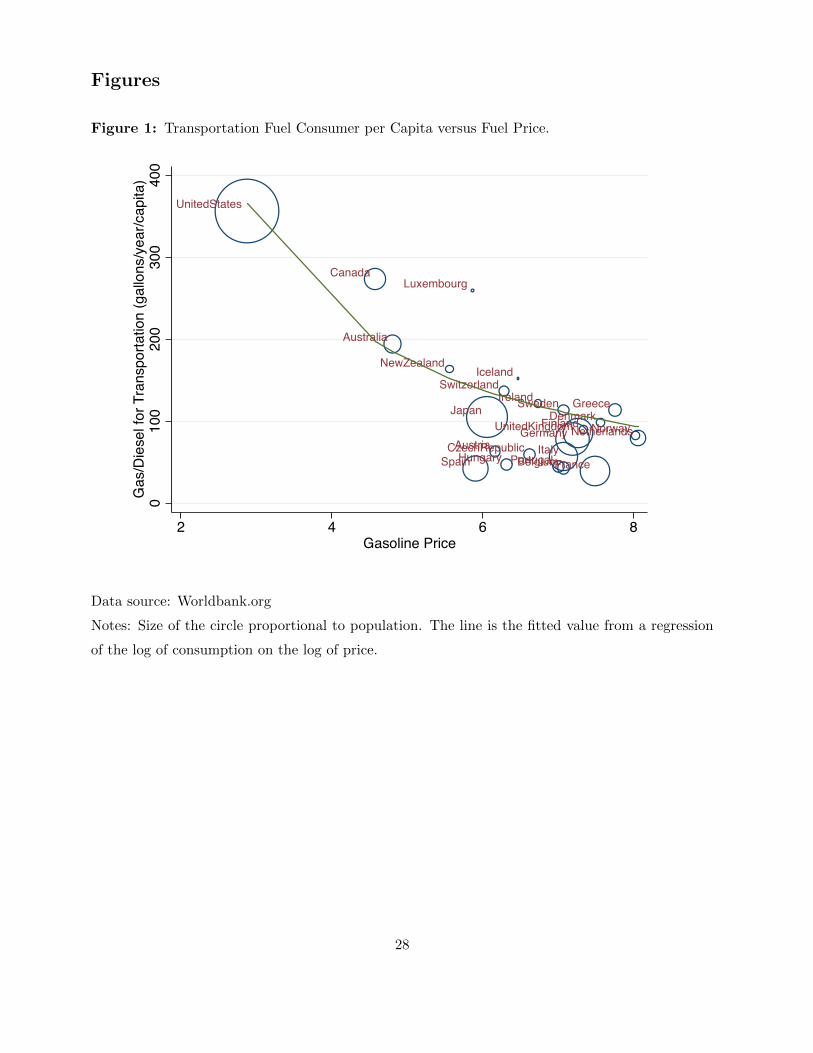
Figures

Figure 1: Transportation Fuel Consumer per Capita versus Fuel Price.

UnitedStates

Canada

Australia

NewZealand

Luxembourg

Spain

Japan

Austria

Switzerland

Hungary

Iceland

CzechRepublic

Ireland

PortugalBelgium

Sweden

Italy

GermanyUnitedKingdomFinland

France

DenmarkGreece

NorwayNetherlands

0100

200

300

400

Gas/D

iesel fo

r T

ransport

ation (

gallo

ns/y

ear/

capita)

2 4 6 8Gasoline Price

!

Data source: Worldbank.org

Notes: Size of the circle proportional to population. The line is the fitted value from a regression

of the log of consumption on the log of price.

28

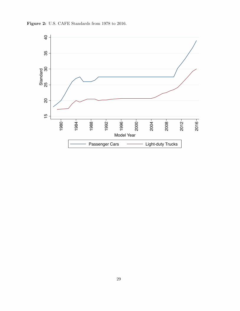
Figure 2: U.S. CAFE Standards from 1978 to 2016.

15

20

25

30

35

40

Sta

ndard

1980

1984

1988

1992

1996

2000

2004

2008

2012

2016

Model Year

Passenger Cars Light-duty Trucks

!

29

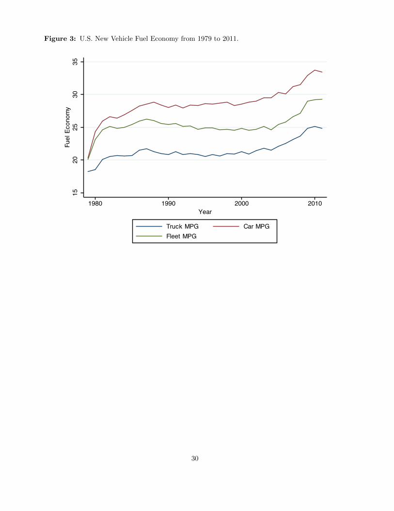
Figure 3: U.S. New Vehicle Fuel Economy from 1979 to 2011.

15

20

25

30

35

Fu

el

Ec

on

om

y

1980 1990 2000 2010

Year

Truck MPG Car MPG

Fleet MPG

!

30

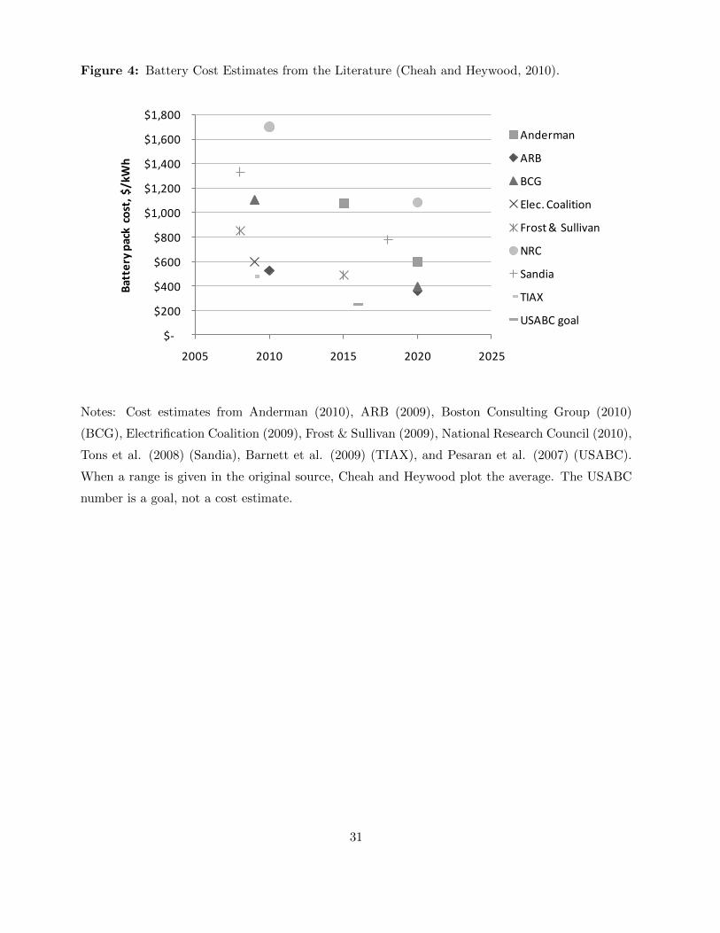
Figure 4: Battery Cost Estimates from the Literature (Cheah and Heywood, 2010).

!"

"

"

!"#$%&'()'*+,"-.,&+'/0'12$#"3'456%"7'8&4"92&+!"#$%&'('$)*+"(*$,-*%),&#$."%/0)'/8&%'9/38&3,"/3.2'8&4"92&+'

"

"

"

!"#$%&':)'*+,"-.,&+'/0';<*='>"?"/3'6.,,&%5'1.9@'9/+,)'A325'-"7?1/"3,+'/0'%.3#&+B'"0'.35B'.%&'12/,,&7)'

" "

#$%&"'()%*+,-

./0"'()%*!,-

1234556"

'()%*+,-

1234556"

'()%*+,-

%(17#)081"

'()%*9,-

#$:"'()%*+,-

#$:"'()%*+,-;24<=">"8?@@ABC5"

'()%*+,-

DE

D9F,,,"

D+F,,,"

DGF,,,"

DHF,,,"

DI,F,,,"

DI9F,,,"

DI+F,,,"

DIGF,,,"

DIHF,,,"

9,,J 9,I, 9,IJ 9,9, 9,9J 9,!, 9,!J 9,+,

C39%&-&3,.2'9/+,'/8&%'9/38&3,"/3.2

DE

D9,,"

D+,,"

DG,,"

DH,,"

DIF,,,"

DIF9,,"

DIF+,,"

DIFG,,"

DIFH,,"

9,,J 9,I, 9,IJ 9,9, 9,9J

D.,,&%5'1.9@'9/+,B'EF@G4

15K62LC5

1$M

M:N

%@6OP":4C@A=A45

;24<=">"8?@@ABC5

#$:

8C5KAC

0/1Q

R81M:"34C@

!

Notes: Cost estimates from Anderman (2010), ARB (2009), Boston Consulting Group (2010)

(BCG), Electrification Coalition (2009), Frost & Sullivan (2009), National Research Council (2010),

Tons et al. (2008) (Sandia), Barnett et al. (2009) (TIAX), and Pesaran et al. (2007) (USABC).

When a range is given in the original source, Cheah and Heywood plot the average. The USABC

number is a goal, not a cost estimate.

31

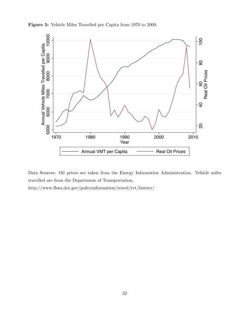
Figure 5: Vehicle Miles Travelled per Capita from 1970 to 2009.

20

40

60

80

100

Real O

il P

rices

5000

6000

7000

8000

9000

10000

Annual V

ehic

le M

iles T

ravelle

d p

er

Capita

1970 1980 1990 2000 2010Year

Annual VMT per Capita Real Oil Prices

!

Data Sources: Oil prices are taken from the Energy Information Administration. Vehicle miles

travelled are from the Department of Transportation,

http://www.fhwa.dot.gov/policyinformation/travel/tvt/history/

32