Reducing Minimum Stock Cover Levels in Fast-Moving Consumer Goods Industry

using Classification Schemes

December, 2015

Maria do Carmo Póvoa

1

Table of Contents Acknowledgements ................................................................................................................. 3

Abstract ................................................................................................................................... 4

Sammanfattning ...................................................................................................................... 5

List of Acronyms ..................................................................................................................... 6

List of Figures ......................................................................................................................... 7

List of Tables ........................................................................................................................... 7

List of Equations ..................................................................................................................... 8

1. Introduction ........................................................................................................................ 9 1.1 A brief historic perspective of Nestlé ................................................................................ 9 1.2 Nestlé Portugal ............................................................................................................. 10 1.3 Context of the Problem .................................................................................................. 11 1.4 Development of the Context of the Problem ................................................................... 12 1.5 Goals of the Thesis’s Work, Research Question and Hypothesis ..................................... 14 1.6 Methodology of the Thesis Work: A First Approach ....................................................... 15

2. Background ....................................................................................................................... 17 2.1 Distribution networks characterization .......................................................................... 17 2.2 Key Performance Indicator ........................................................................................... 18 2.3 Finished Goods Stock Level ........................................................................................... 20 2.4 Stock Policy................................................................................................................... 22 2.5 Basic Concepts: What matters for subsequent work ....................................................... 22

3. State of the Art .................................................................................................................. 23 3.1 Introduction .................................................................................................................. 23 3.2 Specificities of the case under study ............................................................................... 23 3.3 Addressing uncertainty factors related to inventory (Minner 2000) ................................ 23 3.4 Inventory management models (Estellés-Miguel et al. 2012) .......................................... 24 3.5 Stock policies as a component of management (Estellés-Miguel et al. 2012) .................. 25 3.6 Inventory classification in relation of SKU relevance (Ketkar & Vaidya 2014) .............. 25 3.7 Determination of safety stock ......................................................................................... 27 3.8 Addressing the complexity of the case under study with a simple solution (Rojas 2010) .. 31 3.9 Industry sources ............................................................................................................ 31 3.10 Conclusions of the State of the Art ............................................................................... 32

4. Methodology ...................................................................................................................... 34

5. The “Optimizer Tool” ....................................................................................................... 35 5.1 Description of operation ................................................................................................ 35 5.2 How inputs of the “Optimizer Tool” impact stock policies ............................................. 37

6. Analysis of the problem and proposals ............................................................................. 38 6.1 Hypothesis 1 test and validation. Development of insight into how to improve the “Optimizer Tool” ................................................................................................................ 38 6.2 What the insight has revealed to guide the next research steps ....................................... 39 6.3 Hypothesis 2 test and validation: Sensitivity Analysis .................................................... 39

2

6.4 Using classification schemes for the decision support system: answering the research question .............................................................................................................................. 42 6.5 Add-On Development: Classification Schemes and application of their results .............. 43

7. Conclusions and discussion ............................................................................................... 50 7.1 Introduction .................................................................................................................. 50 7.2 Going deeper in to the case study’s results .................................................................... 50 7.3 Conclusion .................................................................................................................... 52

8. Future Work ..................................................................................................................... 53

9. References ......................................................................................................................... 54

Appendix I ............................................................................................................................. 56

Appendix II ........................................................................................................................... 64

3

Acknowledgements

I would like to express my deepest gratitude towards KTH for the great learning journey and international experience through my Master studies. That has been extremely important for my training as a professional, for my development as a person and for my preparation to the reality of this globalized world. Furthermore I would like to thank Nestlé for accepting me for the thesis work and for all subsequent the opportunities that I have been granted to gain practical experience and understanding how a business organization works. It is also fair to acknowledge the importance of my former university, Instituto Superior Técnico, where I got my Bachelor degree, in providing technical capacities and work load management abilities. I also would like to express my appreciation to my KTH supervisor, Lars Lindberg, for all the support, advice, encouragement and engagement through the learning and development process of this master thesis. My recognition includes naturally my Nestlé supervisor, Margarida Melo. In spite of her overwhelming agenda and business responsibilities, she always found time to review my drafts and provide support as well as useful comments and remarks. Besides my Nestlé supervisor, I would like to thank all the team of Demand and Supply Planning that willingly shared their time and experience during the process of gathering information as well as provided feedback. Last, but not the least, I would like to thank my loved ones, family and friends, who supported me throughout the entire process, keeping me motivated. A very special word for my parents whose support was fundamental so that I could have these important experiences that made me wealthier in terms of culture, spirit and developed the possibility of being a good professional. I will be forever grateful for their love and support.

4

Abstract This thesis was developed at the Demand and Supply Planning department (DSP) of Nestlé Portugal whose mission is to develop planning scenarios encompassing the whole supply, production and distribution cycle to support the most appropriate decisions at each operational level. Stock policies are among the most important parameters that DSP defines periodically. Such parameter includes minimum and maximum stock cover levels. The minimum stock cover levels tell how many days the stock will last if demand goes as predicted. From that value the maximum stock cover levels is then calculated and stock policies are set. Currently stock cover policies are defined by Supply Planners with a home built tool called “Optimizer Tool” that shows overestimation. This situation implies extra cost and inefficiencies that the company wants to address by the present thesis work. After study of the context and specificities of the situation the goals agreed were: 1) Complement “Optimizer Tool” operation with an innovative process to reduce the suggested minimum stock cover levels. 2) Develop a case study based on “Optimizer Tool” routine operation for demonstration purposes. For reasons associated namely with confidentiality issues the approach used was mostly empirical, in the sense that no analysis of fundamentals of the “Optimizer Tool” was undertaken. On that line of work, after considering that stock policies are indeed the result of the interaction between “Optimizer Tool” operation with human judgement on several inputs that can be adjusted, the research question to meet the objectives was: How to optimize the integration of “Optimizer Tool” operation with the inherent human judgement? This question was based upon two hypothesis that were formulated, tested and validated. The literature review showed that classification schemes for the individual items (Stock Keeping Units or SKU’s for Nestlé) could be used with the Simple Additive Weighting (SAW) methodology in the search of a solution to the problem under study. Furthermore, it was clear that addressing uncertainty factors related to inventory could be based on what was called the rolling horizon framework (basically, learn as you go). These findings lead to the development of a tool or add-on putting together classification schemes and a learn as you go process. The validation of the hypothesis mentioned above was then performed. That included a sensitivity analysis that made clear that the options made by Supply Planners when using the “Optimizer Tool” in respect to two inputs, the so called Adjusted Demand Plan Accuracy (DPA) and Adjusted Master Schedule Attainment (MSA), were critical to the quality of results in terms of stock policies. A specific set of classification schemes was then developed and combined with SAW methodology in three different arrangements. The combination schemes were prepared to be applied to the final results of an “Optimizer Tool” run. That option was dictated by the existence of company targets for Adjusted DPA and Adjusted MSA (that in principle should be adopted). Additionally, such option keeps present operation of the system totally unchanged, just introducing a reference that allows a deeper analysis in respect to stock policies (as illustrated in the case study and subsequent discussion). The case study was successful and the possibility of taking sound decisions on keeping or reducing minimum stock cover levels was demonstrated. It should be noted that the tool or add-on is not a substitute of human experience and knowledge. It is a support to a more informed decision. Furthermore it opens new possibilities in respect to formalization, sharing, continuous learning and adaptation to new conditions, in line with the rolling horizon framework of addressing uncertainty factors in respect to inventory. Keywords: Stock; Stock Management; Stock Policy; SKU Classification

5

Sammanfattning Examensarbetet är utfört på ”Demand and Supply Planning department” (DSP) på Nestlé, Portugal. Avdelningen ansvarar för scenarioplanering för inköp, produktion och distribution som underlag för beslutsfattande. Lagerstyrning är en av de viktigaste faktorerna som regelbundet definieras av DSP. Parametrar som ingår i lagerstyrningen är bland annat lägsta och högsta lagernivån. Den lägsta nivån anger hur länge lagret räcker ifall efterfrågan utvecklas som förutspått. Utifrån de värdena kan man beräkna högsta lagernivån och därmed fastställa lagerstyrningspolicy. I dag definieras policyn av inköpsavdelningen, som använder sig av ett egenutvecklat verktyg, ”Optimizer Tool”. Problemet är att verktyget överskattar den lagernivå som krävs. Företaget vill komma till rätta med detta problem genom detta examensarbete. Efter en förstudie av nuläget sattes två mål upp: 1) Komplettera ”Optimizer Tool” med en ny metod för att reducera den lägsta lagernivån. 2) Utarbeta en fallstudie baserad på rutinerna i användningen av ”Optimizer Tool” för framtida demonstrations ändamål. Ingen analys av de grundläggande funktionerna i ”Optimizer Tool” kunde genomföras på grund av sekretesskäl. Istället användes empirisk data. Efter att på vissa punkter ha fastställt sambandet mellan verktygets resultat och människors bedömningsförmåga kunde forskningsfrågan fastställas: Hur kan man optimera integrationen av resultaten från ”Optimizer Tool” processer med den mänskliga bedömningsförmågan? Denna fråga baserades på två hypoteser som utformades, testades och validerades. Litteraturstudien visade att klassifikationssystemen för de individuella produkterna (Stock Keeping Units eller SKU:s) kunde användas tillsammans med Simple Additive Weighting (SAW) metoden för att lösa problemet i fråga. Det var också tydligt att osäkerheten i lagerstatus kunde åtgärdas med den så kallade ”rolling horizon framework” som i princip går ut på att läras sig efter hand som man gör. Dessa insikter ledde till utformningen av ett verktyg eller tillägg som kombinerade klassifikationssystem med en lära genom att göra process. Efteråt utfördes valideringen av den ovan nämnda hypotesen. Valideringen bestod delvis av en känslighetsanalys som gjorde klart att det var två ingående värden som hade störst inverkan på lagerstyrningen när personalen använde ”Optimizer Tool”: Adjusted Demand Plan Accuracy (DPA) och Adjusted Master Schedule Attainment (MSA). Därefter konstruerades ett specifikt klassifikationssystem vilka kombinerades med hjälp av SAW metoden i tre olika varianter. De kombinerade systemens anpassades för att appliceras på det slutgiltiga resultatet av en ”Optimizer Tool” körning. Den möjligheten bestämdes av företagets mål för Adjusted DPA och Adjusted MSA (som i princip skulle ha anpassats). Sådana möjligheter förändrar inte de aktuella processerna i systemet. Istället introducerar de en referens för djupare analyser av lagerstyrning (som framgick i fallstudien och den tillhörande diskussionen). Fallstudien var lyckad och möjligheten att göra avvägda beslut i frågan om den lägsta lagernivån presenterades. Det är värt att notera att verktyget eller tillägget inte ska ses som en ersättning för personalens erfarenhet och kunskap, utan ett extra stöd i beslutfattandet. Den öppnar även nya möjligheter för formalisering, delning, kontinuerligt lärande och flexibilitet i förhållande till ” rolling horizon framework” ansatsen till problemlösning av osäkra faktorer av lagerstatus.

6

List of Acronyms CAPDo Check Act Plan Do CFR Case Fill Rate CPW Cereal Partners Worldwide DPA M-1 Demand Plan Accuracy DSP Demand and Supply Planning F Forecast FMCG Fast-Moving Consumer Goods FSN Fast – Slow – Non-moving HML High – Medium – Low KPI Key Performance Indicator L Lead-Time MSA Master Schedule Attainment NNS Nestlé Net Sales OC Order Cycle OP Order Point PF Percent Fill PUM Planning Unit Measure Q Quantity QA Quality Assurance R&G Roast & Ground SAP Systems, Application & Products in Data Processing SAW Simple Additive Weighting SDE Scarce – Difficult - Easy SKU Stock Keeping Unit SS Safety Stock TNWC Trade Net Working Capital WAPE Weightned Absolute Percentage Error WWI World War I WWII World War II 3PL Third-Party Logistics

7

List of Figures

Figure 1 - Demand and Supply Structure (Nestlé 2014a) 11 Figure 2 - Inventory Costs and Service Level Relationship (Nguyen 2014) 13 Figure 3 - CAPDo Approach (Macca 2012) 13 Figure 4 - Delivered PUMs in 2014 (Nestlé 2015) 16 Figure 5 - Mono-Echelon Network (Nguyen 2014) 17 Figure 6 - Multi-Echelon Network (Nguyen 2014) 17 Figure 7 - Where KPI’s are calculated 18 Figure 8 - Components of Finished Goods Stock (Nguyen 2014) 20 Figure 9 Relationship between Minimum Stock Cover and Demand Plan Accuracy (Macca 2012) 21 Figure 10 Cycle Stock (Macca 2012) 21 Figure 11 - “Optimizer Tool” Scheme of Operation 35 Figure 12 - Results of sensitivity analysis of “Optimizer Tool” output with 25% decrease on inputs

41 Figure 13- Results of sensitivity analysis of “Optimizer Tool” output with 25% increase on inputs 41 Figure 14 – SKU W Calculation 64 Figure 15 – SKU X Calculation 65 Figure 16 – SKU Y Calculation 66 Figure 17 – SKU Z Calculation 67

List of Tables

Table 1 - Assigning Weight to the Classification Schemes 26 Table 2- Classification Values to the different Schemes 26 Table 3 - Examples of outputs from “Optimizer Tool” and Supply Planners’ decision regarding

minimum stock cover level 40 Table 4 - Classification Schemes to use in the add-on 44 Table 5 - Criteria for attribution of points on each classification scheme 45 Table 6 - Suggestions of percentage weights for SAW methodology 45 Table 7 - Points of each SKU in relation to classification schemes based on past data methodology 46 Table 8 - Application of maximum points of each classification scheme to the suggested weights 46 Table 9 - Application of SKU W points of each classification scheme to the suggested weights 47 Table 10 - Application of SKU X points of each classification scheme to the suggested weights 47 Table 11 - Application of SKU Y points of each classification scheme to the suggested weights 47 Table 12 - Application of SKU Z points of each classification scheme to the suggested weights 48 Table 13 - Balanced classification for each SKU (SAW methodology) expressed as percentage of the

maximum classification for three suggestions of weighting 48 Table 14 - Application of add-on to “Optimizer Tool” using historical values for adjusted DPA and

adjusted MSA 49 Table 15 - Application of add-on to “Optimizer Tool” using target values for adjusted DPA and

adjusted MSA 49 Table 15 - Application of add-on as decision support system: Results 52 Table 16 - Sensitivity Analysis +25% for SKU W 56 Table 17 - Sensitivity Analysis +25% for SKU X 57 Table 18 - Sensitivity Analysis +25% for SKU Y 58 Table 19 - Sensitivity Analysis +25% for SKU Z 59

8

Table 20 - Sensitivity Analysis -25% for SKU W 60 Table 20 - Sensitivity Analysis -25% for SKU X 61 Table 20 - Sensitivity Analysis -25% for SKU Y 62 Table 20 - Sensitivity Analysis -25% for SKU Z 63

List of Equations

Equation 1 DPA M-1 Calculation 19 Equation 2 TNWC Calculation 20 Equation 3 - Classification Number Calculation 27 Equation 4 - Safety Stock Calculation (Schönsleben’s) 27 Equation 5 - Coefficient of Variation Calculation (Schönsleben’s) 28 Equation 6 - Calculation if Demand is Normally Distributed 28 Equation 7 - Percent Fill Calculation 28 Equation 8 - Safety Stock Calculation (Thomopoulo´s); Option 1 28 Equation 9 - Standard Deviation Of Demand over Lead-time 28 Equation 10 - Expected Demand exceeding OP during OC 29 Equation 11 - Coefficient of Variation Calculation (Thomopoulo´s) 29 Equation 12 - Expected Demand Calculation 29 Equation 13 - Safety Stock Calculation (Thomopoulo´s); Option 2 29 Equation 14 - Forecast Error Calculation 30 Equation 15 - Forecast Accuracy Calculation 30 Equation 16 - Weighted Absolute Percentage Error 30 Equation 17 - Forecast Error Calculation in Percentage 30 Equation 18 - Forecast Error Calculation in Percentage for Nestlé 30 Equation 19 - Root Mean Square Error Calculation 31 Equation 20 - Safety Stock Calculation (Chockalingam's) 31

9

1. Introduction

1.1 A brief historic perspective of Nestlé In 1866 the Anglo-Swiss Condensed Milk Co. S.A., the first condensed milk company in Europe, was founded in Cham (Switzerland) by two American brothers. In 1867 Henri Nestlé, a chemist with interest in instant formulas and founder of a company that bears his name, launched Farine lactée, setting dairy based nutrition as the core business of the company. In 1905 the Anglo-Swiss Condensed Milk Company merged with Nestlé putting an end to years of intense competition. Some years later, when the First World War (WWI) started, the new company faced a big challenge. As a matter of fact, the conflict brought major difficulties for the whole supply chain: raw materials were difficult to get and it was hard to distribute finished products. But after a while the problem turned out to be a great business opportunity: the need for food items, something Nestlé was able to provide. That led to many contracts and an increase of demand for the company’s dairy products. By the end of the war Nestlé had 40 factories worldwide. Later, the economic crisis of the 20’s of last century hit Nestlé, but nevertheless it managed to keep growing through acquisitions: Cailler, Peter and Kohler Swiss Chocolate Company. Not surprisingly, chocolate became then an important part of Nestlé’s business. In short, after a period of growth during WWI, as the market suffered a downturn, Nestlé’s growth continued but in the form of mergers and acquisitions in business areas where the company had some know how. This process led to a diversification of products and therefore gave Nestlé new opportunities to develop further growth. In the late 30’s to early 40’s the company made a step outside the dairy sector with the launch of Nescafé (1938) and of Nestea (1940). Another global conflict, the Second World War (WWII), created a huge demand for some of the company’s products, like Nescafé. The post-war marked a dynamic phase for the company, with a combination of acquisitions to be achieved and new products to be launched. For instance, Nestlé acquired Maggi products (1947), launched Nesquik (1948) and became a major shareholder in L’Oréal (1974). So it is interesting to see that both WWI and WWII brought important opportunities for growth, based on products that in both cases were developed just some time before, and that were important in the logistics supporting warfare. After the conflicts Nestlé grew also by a mergers and acquisitions and by product diversification. From the mid 70’s to the mid 1980’s Nestlé suffered a setback, when many consumers agreed to boycott the company’s products as a protest against aggressive marketing practices. Those practices were pushing the use of breast milk substitute, regardless of health concerns. The boycott was cancelled in 1984 after the company agreed to abide by terms of the International Code for the Marketing of Breast-milk Substitutes. Many companies faced similar challenges at the time, when consumers’ organizations began to appear and have clout. From then on, consumers’ attitude has been growing in importance as part of any company’s strategy. In spite of the boycott, Nestlé continued to grow along the two drivers identified above. For instance in 1986 Nespresso brand was created and in 1988 Nestlé acquired Buitoni, a major italian food brand.

10

In this century (2001) Nestlé entered into the market of animal nutrition, by merging with Ralston Purina Company to form Nestlé Purin PetCare Company. The list of acquisitions made since then includes Novartis Medical Nutrition (2007), Kraft Foods frozen pizza business (2010) and Wyeth Nutrition (from Pfizer Nutrition in 2012). (Nestlé n.d.) As a result Nestlé operates worldwide in many areas of business related to nutrition, although its interests include other sectors. The company has 447 factories in 86 countries and operates in 196 different countries. Its products are constantly being improved or innovated at 34 research centers. All of this is managed by 339 thousand employees. Beyond what the figures tell, Nestlé is a well-known brand that consumers associate with quality, trust and safety. A major asset when it comes to sell food. (Nestlé 2014c)

1.2 Nestlé Portugal In 1933 a factory of milk products, built in Avanca, was awarded the exclusive right of producing and selling of Nestlé products. In 1948 Maggi products were introduced into the Portuguese market and 10 years after the same happened to Nescafé. In the early 70’s the level of business growth led to the creation of a branch of Nestlé in Portugal. That supported the creation of new business areas, moving production lines to the country, as well as the acquisition of companies such as a chocolate factory, coffee roasters and a yogurt producer. Simultaneously, Nestlé Portugal supported the introduction of several products in the national market like Nestea (1994), Nestlé Purina Pet-Care (2002) and Nespresso (2003). In 2008 the company celebrated the 85th birthday of its operations in Portugal. (P. Nestlé n.d.) Nestlé Portugal is now a reference company in the country. Besides its headquarters located in Linda-a-Velha, as of 2013 Nestlé Portugal manages 4 factories and 17 distribution centers, as well as work force of 1869 employees. In 2013 the turnover was 471,3 Million €. The share of the turnover associated with exports was roughly 19% (88,5 Million €). (Nestlé 2014c) The success of Nestlé Portugal made it convenient to create several business areas:

Dairy and Cereals Coffee & Beverages Chocolates and Confectionary Ice Cream Culinary Roasted & Ground (R&G) Coffee (which includes Branded Food and Branded Beverages

– Food for professionals, such as Hotels and Restaurants) Infant Nutrition Cereals Partners Worldwide (CPW)

Petcare and Nespresso are not included in the list, since they are operated differently within the company.

11

1.3 Context of the Problem The responsibility of DSP department of Nestlé Portugal is to develop planning scenarios for each Stock Keeping Unit1 (SKU) encompassing the whole supply, production and distribution cycle to support the most appropriate decisions at each operational level. Additionally DSP is responsible to follow up planned implementation, managing unexpected situation as they unfold, to ensure that company’s goals are met. Figure 1 shows the scope of responsibilities and functions of DSP department within Nestlé Portugal. (Nestlé 2014a) The figure shows a two dimensional structure that is relevant to understand the complexity of the above mentioned planning and managing process:

- Vertically the figure has a time-line, from strategic (years) to execution (weeks) - Horizontally it is clear the cross cutting nature of DSP interaction, from procurement to

customer DSP has a Supply Planner2 for each business area (refer to section 1.2 on Nestlé Portugal) whose functions include:

- contribute to the planning process mainly by defining stock cover levels for the SKUs under their responsibility based on projections of demand (provided by the respective Demand Planner2)

- develop efficient and effective responses to deviations of the planning scenarios (between plan reviews)

The time scope of DSP planning is 18 months, but on a weekly basis there is an update of forecasts and a review of the existing plan, from production to distribution to meet the stock cover levels initially defined. (Nestlé 2014d)

1 A Stock Keeping Unit is any item from a group of items with the same product identification number. In short it is the unit of a specific product that can be sold to final customers. 2 Each business area has its Demand Planner and its Supply Planner. The latter takes the necessary actions to meet the needs of the former.

Figure 1 - Demand and Supply Structure (Nestlé 2014a)

12

The performance of each business area is assessed using pre-defined Key Performance Indicators (KPI), whose targets are defined on a yearly basis. Their results are aggregated according to Nestlé Portugal’s own criteria to determine overall performance in the same period. There are four major KPIs in relation to DSP scope of activity: Demand Plan Accuracy (DPA M-1)3, Bias, Stock Cover and Case Fill Rate (CFR). A short definition of terms is given for the sake of clarity (a complete definition is given at the Key Performance Indicator section):

- DPA M-1 refers how close predictions are matching reality one month ahead (M-1); - Bias is related to deviations of the demand; - Stock cover tells how many days the stock will last if demand goes as predicted; - CFR reveals how well customers’ needs are being met.

In the context of the present work, stock cover is the most important KPI that evaluates the effectiveness of stock cover policies. A stock cover policy for a particular SKU is defined by a minimum and a maximum stock cover. The defined interval of stock cover represents the desired working range for DSP, to avoid over and out of stock situations. Currently stock cover policies are defined by Supply Planners with a tool developed in-house called “Optimizer Tool”. The tool is quite handy since it eases dealing with historical data, demand projections and sets several parameters automatically. However it tends to overestimate what is needed in addition to the minimum stock cover. Nestlé Portugal has a limited warehouse area, so overstock situations will lead directly to the rental of an external warehouse (3PL), which adds more costs to those caused by excess in inventory. This situation is the problem DSP is facing since in order to have a better performance and to reach the defined goals it needs more accurate results from the above mentioned tool. Finding the way to have more accurate results will reduce wastes, ease the path to reach goals and avoid unnecessary risks for the supply chain. The optimal scenario, and that DSP wishes that this work may contribute is to reduce the minimum stock cover level, without jeopardizing the service level.

1.4 Development of the Context of the Problem 1.4.1 Check Act Plan Do (CAPDo) Approach The ultimate goal in optimization of inventory (i.e., stock level of a particular SKU) is finding the right balance between minimization of inventory costs and maximization of service level for each SKU. Figure 2 illustrates the trade-off between those two factors. From the relationship established it is possible to understand that a higher customer service level implies higher inventory costs. Nevertheless sacrificing either factor is not an option. As a matter of fact, reducing inventory costs beyond a certain point brings customer service to inacceptable levels. Therefore optimization process involves identifying all the drivers and processes to improve the efficiency of the overall system while keeping costs and service within acceptable levels.

3 DPA is a measure of accuracy of a plan, which in the present case will be determined with one month of anticipation: M-1. Therefore DPA M-1 will be used.

13

Several arrangements of the overall system will show different curves as well as trade-offs and a theoretical iterative process can be pursued to achieve the highest service level at the lowest inventory cost. (Nguyen 2014) Nestlé’s DSP approach to optimize the finished goods inventory is CAPDo. This is a well-known continuous improvement methodology where the 4 steps (Check, Act, Plan and Do) have been adapted to the particular needs of inventory optimization. The Check step implies a periodical review of the stock cover, inventory freshness and stock service to identify improvement areas, such as gaps and obsolete inventory. The Act step regards understanding the behavior of the different stock components and their drivers. That is where the “Optimizer Tool” comes in whenever needed. As a matter of fact, it may happen that there is underperformance on KPIs that are not affected by the “Optimizer Tool” output. After this analysis improvement opportunities are addressed and, if the “Optimizer Tool” is used, new stock policies can be defined (refer to section 1.3 on Context of the Problem).

Figure 3 - CAPDo Approach (Macca 2012)

The Plan step is next with a cross-functional action plan being designed. Responsibilities, timelines and expected results are defined at this stage. Finally in the Do step the action plan is

Figure 2 - Inventory Costs and Service Level Relationship (Nguyen 2014)

14

carried out, with improved control and evaluation of the performance considering stock cover, stock service and inventory freshness. The above described approach is sketched in the Figure 3. It is possible to understand that it is an iterative approach. This approach encompasses all that is needed to improve the inventory management cycle. Since it is an iterative process it can be perceived as an ongoing journey of continuous optimization. (Macca 2012) The coordination of this approach is ensured by periodical meetings of DSP managers with all other entities involved. Those meetings can be scheduled daily, weekly or monthly considering the requirements of the different operational levels. Besides coordination, this process allows also communication and identification of gaps. 1.4.2 The importance of the “Optimizer Tool” for inventory optimization From the above description it is clear that the “Optimizer Tool” holds a very important role to achieve the desired continuous improvement in terms of inventory management. Without it, working through the huge amount of available data related to each SKU to deliver guidelines for inventory management would be a time and resource consuming task. Besides efficiency of data processing, that home built tool helps to find opportunities for cost reduction. As a matter of fact, an ideal supply chain should deliver the right product, in the right quantity and quality at the right time to the customer keeping overall cost to a minimum. And, all other factors being equal, cost minimization opportunities within a supply chain rely mostly in inventory management, as costs from production, transportation, etc. are comparatively more difficult to improve. Inventory inefficiencies may occur for instance if SKU’s are stored for too long. But risk of waste is not the only problem in managing inventory levels. Inventories have a cost, as storing SKU’s takes capital, and so it will not be used in other purposes such as investment in other activities. The more capital is tied up as inventory, the less will be used. A systematic approach reveals other costs related to this activity. As referred there is the capital that is not invested in order to have a certain level of inventory, the opportunity cost. Additionally there are carrying costs, the costs of handling the inventory such as storage, wages and equipment costs. Obsolescence costs have also to be considered in this case, that occur when the products do not meet the minimum of the freshness levels required. On the other hand, if demand is not satisfied by the inventory there will be stock-out costs. The impact of this situation may lead to different consequences. Besides the profit of the sale that would be generated, the reputation of the company may be damaged and future sales may be reduced. (Nguyen 2014) That is the challenge that the “Optimizer Tool” addresses to contribute to an efficient management of a supply chain (considering the given distribution network – with just one distribution center)

1.5 Goals of the Thesis’s Work, Research Question and Hypothesis

Considering the above described problem the thesis addresses the improvement intended by DSP following a two-fold approach:

15

1. Complement “Optimizer Tool” operation with an innovative process to reduce the suggested minimum stock cover levels for SKU’s.

2. Develop a case study based on “Optimizer Tool” routine operation for a selected set of SKU’s for demonstration purposes.

For a better explanation of the goals of thesis work, the relationship that exists in calculation of stock policies (minimum and maximum stock cover levels) and of minimum stock cover levels should be highlighted. The latter is a direct result of the “Optimizer Tool” (and can be adjusted). From that value the maximum stock cover level is then calculated and stock policies are set. From the previous sections it becomes clear that the “Optimizer Tool” has to integrate a large set of inputs that are representative of the supply chain of each SKU, from production till Nestlé customers. As it will be explained in section 5, where a description of how the user operates the system is provided, the Supply Planner is supposed to use his or her knowledge and expectations to adjust several variables. Therefore the “Optimizer Tool” final results are in fact a combination of automatic calculation and human judgement. It is out of the scope of this work to perform an analytical approach to the “Optimizer Tool” algorithm and calculations that are the result of years of experience, linking theory with practice. Moreover that approach would be incompatible with the available timeframe. Human judgement is indeed of great importance when it comes to incorporate efficiently and effectively a complex set of uncertainties, associated with the likelihood of scenarios defined by the risk of events (e.g., problems in a factory) and/or possible decisions from third parties (eg, identification of marketing opportunities) regarding each SKU. This interaction between the “Optimizer Tool” and human judgement deserves to be investigated. In this context the research question that has to be addressed to meet the objectives is: How to optimize the integration of “Optimizer Tool” operation with the inherent human judgement? This research question is supported by the following two hypothesis: H1: There is no detectable problem in “Optimizer Tool” operation that recommends a specific reformulation of any of its modules. H2: The variables that the Supply Planner is allowed to adjust have great influence on the “Optimizer Tool” final results. The first hypothesis will be tested by working with the tool, using an extensive set of real life data from Nestlé’s historical records. The absence of symptoms of lack of soundness on results, instability or ineffectiveness will be taken as a confirmation that H1 is corroborated. The second hypothesis will be tested with a sensitivity analysis of the “Optimizer Tool”. That will be done with an increase or a decrease of each input that the Supply Planner use, while keeping all others constant, with the purpose of determining qualitatively (or ranking) which of those inputs have the greatest impact on “Optimizer Tool” final results. If the variables the Supply Planner can adjust by using his or her judgement are those to which sensitivity is higher, then it can be assumed that H2 is corroborated.

1.6 Methodology of the Thesis Work: A First Approach Assuming the hypothesis formulated above are validated, the methodology of the work to answer the research question and deliver what is required by DSP can be separated into two phases.

16

In the first phase, a complement (or add-on) to the “Optimizer Tool” will be implemented, based on the results from the literature review. As a matter of fact, the complexity of the “Optimizer Tool” imposed some limitations to the implementation as well as to the test of the modifications in the scope of this thesis work. In respect to the second phase, it is worth considering Figure 4, taken from the report of Stock in 2014, where each color corresponds to the Planning Unit Measures4 (PUM’s) a business area delivered during that year. In other words, the greater the PUM the more boxes a business area moved within the considered supply chain. (Nestlé 2015) Percentages are not indicated due to confidentiality reasons.

Figure 4 - Delivered PUMs in 2014 (Nestlé 2015)

As it can be perceived, Beverages and Dairy and Cereals are the business areas that deliver nearly half of the PUM’s in 2014. Among these two business areas, the Cereals component (of Dairy and Cereals business area) is presently the most challenging, because of the high frequency that is occurring of overstock situations. Moreover that situation involves three SKU’s that are extremely relevant for turnover. The second phase of the thesis’s work will be a case study where the “Optimizer Tool” complement (or add-on) will be tested on some SKU of the Cereals category.

4 A PUM is a package of SKU (items with same product identification number) for logistic purposes. A PUM of a particular SKU has always the same number of items.

17

2. Background

2.1 Distribution networks characterization Nestlé takes part in the Fast Moving Consumer Goods (FMCG) industry. In the food sector it is crucial to run stocks of finished goods efficiently since this industry requires a good service level avoiding at the same time any waste. Indeed, excess inventory is not only a liability due to tied up space and capital but also because it soon becomes deteriorated. Freshness is therefore a characteristic to take into account in the food sector inventory. In the case of Nestlé products can only be sold in the first trimester of their total shelf life in the retail channel. After this period the product is blocked in the inventory and can only be sold with a smaller profit. The part of the inventory that becomes blocked, as mentioned above, on the account of its age is called salvage. Setting freshness as an issue to address in inventory management improves a better finished good policy and simultaneously ensures the highest quality of Nestlé products get to the customers. (Macca 2012) Freshness of the inventory is therefore one of the most important KPI, that will be defined in the following section together with other relevant indicators. Such information allows tracking performance on a common basis for the two main types of distribution network that make sure the products flow to the point of sale. Two types of distribution networks should then be considered: mono-echelon and multi-echelon. In a mono-echelon network (Figure 5), the products flow from the factory to one or more Distributions Centers and then are sold to the customers through different retails channels. (Macca 2012)

In a multi-echelon network (Figure 6) the finished goods are first shipped to a Central Distribution Center. Afterwards they are transported to other Distribution Centers and then, through a retail channel, to the costumers. The multi echelon is more complex and therefore more difficult to optimize. (Macca 2012)

Figure 6 - Multi-Echelon Network (Nguyen 2014)

Figure 5 - Mono-Echelon Network (Nguyen 2014)

18

In Nestlé Portugal the only business area that has a multi-echelon network structure is the R&G Coffee. The reason for such arrangement is that this business area includes van sales and delivery directly at the final costumer (R&G coffee shops). Moreover, this segment has a frequent need to deliver orders to the final customers.

2.2 Key Performance Indicator As stated before, KPI’s are used to track and compare the efficiency and effectiveness of management practices within the inventory. Therefore measuring and monitoring those indicators is instrumental to assess how well a company is doing and to identify where improvements can be done. There is a set of 11 major Supply Chain Key Performance Indicators agreed. (Nguyen 2014) The following figure will be helpful in the definition of the operational KPI’s.

Figure 7 - Where KPI’s are calculated

1. Case Fill Rate (CFR)

This indicator assesses the service level. It represents the number of orders completed and delivered by Nestlé against the number of orders submitted by its customers. This is the KPI that Nestlé uses to evaluate how well customers’ needs are being met. For the sake of clarity, a Nestlé customer is an external business organization that will sell products to the final consumer.

2. Stock Cover Stock cover is the most popular KPI, since it may assist in preventing overstock scenarios. Stock cover is the number of days for which finished goods at any given moment will last against the Demand Plan for the following months. From this number it is possible to know the quantity and value of the inventory. The minimum stock cover should give the demand planner a safe solution of stock to avoid out of stock situations.

19

3. Freshness Inventory

As mentioned Nestlé is a FMCG industry and therefore all finished goods have a given shelf life. This indicator shows the remaining shelf life of the inventory. This is an important KPI to consider within the inventory since its value may make the product non-saleable. After one third of its shelf life the stock is marked as non-saleable (except in special conditions where it becomes saleable but less profitable).

4. Demand Plan Accuracy (DPA M-1) The forecast of the demand used by the DSP department has associated uncertainties. The indicator evaluates the quality of the demand plan on a monthly basis. It is calculated for each business area by summing the absolute value of the differences between the demand predicted by the plan for each SKU and the corresponding actual demand. After the sum, the value is divided by the sum of the demand planned for the same period. The formula is shown in the Equation 1. In the present case the calculation is intended to determine how predictions are matching reality one month ahead (hence M-1).

5. Master Schedule Attribute (MSA)

MSA shows how accurately production has met the agreed quantities on a weekly basis expressed as percentage. This indicator helps to assess the problem arising from supply uncertainty. If this KPI is low the inventory levels will have to be higher to avoid stock out scenario and similar problems that may occur.

6. Stock Service As the service level towards costumers is evaluated so is the stock service, specifically the performance of inter-market supply chains. This KPI evaluates the stock service within Nestlé between producing and receiving business-to-business markets.

7. On Shelf Availability (OSA) This KPI aims to evaluate if every time a final consumer desires a product, the required product is available at the right time and place. On Shelf Availability is calculated by the difference between the items available at a particular location and the total items that are required there.

8. Dispatch Schedule Attainment (DSA) DSA evaluates the performance of the domestic supply chain, between factories, the Central Distribution Centers and the receiving locations. It measures the behavior of the supply chain in transportation related issues.

Equation 1 DPA M-1 Calculation

20

9. Freshness of Shipments As previously mentioned, freshness is an important issue to address moreover as Nestlé takes part in the FMCG industry. This freshness indicator provides the average remaining shelf life at the time of shipment to costumers.

10. DPA Bias The DPA Bias identifies the significant under and over demand forecasts plans.

11. Production Frequency Report This is a KPI provided by production facilities. It is the average number of days between two subsequent production runs of a particular SKU during of a selected time frame. It is important to determine how much to produce each time.

12. Trade Net Working Capital as % Nestlé Net Sales (TNWC as % of NNS) Trade Net Working Capital refers to the financial well-being of the company, and for this KPI is expressed as a percentage of Nestlé Net Sales. (Nguyen 2014)

푇푁푊퐶 = 푅푒푐푒푖푣푎푏푙푒푠 + 퐼푛푣푒푛푡표푟푖푒푠 − 푃푎푦푎푏푙푒푠

Equation 2 TNWC Calculation

Final remark: The KPI’s more frequently used by DSP are DPA M-1, Stock Cover, Bias, CFR, and Freshness. (Nestlé 2014b)

2.3 Finished Goods Stock Level There are different types of inventory to be considered within a supply chain: raw materials, in-process products, purchased parts and supplies, components parts and finished goods. In the scope of this work only finished goods are taken into account. Within the finished goods stock, there are different components to consider: safety stock, pipeline stock, cycle stock and stock build (Macca 2012). In figure 8 it is possible to see how the different components of the finished goods can vary with time.

Pipeline stock (Blue color in Figure 8) is the stock that covers products that are still in production process, transportation or in incubation for quality reasons. Consequently, this stock component

Figure 8 - Components of Finished Goods Stock (Nguyen 2014)

21

is not immediately available for sale. The main drivers of this type of stock are the quality assurance release time, the distance between the producing and receiving location and the administrative lead time. Considering uncertainties of supply, lead time and demand there is the need for a safety stock (Orange color in Figure 8). It ensures the system capability to withstand uncertainty and achieve the targeted customer service level (mentioned as KPI CFR). In Figure 9 it is possible to understand the trade-off between demand plan accuracy, customer service level and minimum safety stock. Low demand plan accuracy, when targeting a high customer service level forces the company to have a high safety inventory. (Macca 2012)

Customer service level and demand plan accuracy are the most important drivers for this type of stock. Other factors that determine safety stock are the number of warehouses and the variability of the transit time between producing and receiving location. The cycle stock (Green color in Figure 7) is related to the production cycle and also delivery frequencies as well as minimum production and transportation quantities. Production is not made continuously but in batches, which introduces an inventory pattern illustrated in Figure 9.

Build stock (Red color in Figure 7) covers situations where the demand is known to increase for one of the following reasons: product seasonal demand; product promotion. It also covers situations where supply is expected to decrease for instance because of production capacity

Figure 9 Relationship between Minimum Stock Cover and Demand Plan Accuracy (Macca 2012)

Figure 10 Cycle Stock (Macca 2012)

22

constraints or factory shutdown. In either case, products are manufactured in anticipation to those scenarios. Slack stock is not considered as a component from the finished good stock levels since it is unnecessary stock. Slack stock is defined as the part of the stock that cannot be explained by the parameters of the supply chain. The identification of slack stock allows the evaluation of the performance of the supply chain. (Macca 2012)

2.4 Stock Policy The stock policy matches the management decisions on the level of inventory to be held by the company. Each SKU has its own stock policy, considering that service level target is taking into account all uncertainties. The stock policy is the minimum and the maximum stock cover levels (where the latter is a function of the former). When the value of days of demand coverage goes below the minimum stock cover it triggers the replenishment process. The minimum stock cover represents the inventory level that fulfills all needs, considering the possible constraints caused by the Demand and Supply uncertainty and ensures a certain service level. The maximum stock cover is an indicator that shows the maximum inventory that should be held but it does not influence the inventory levels. It considers the storage constraints and freshness issues that may arise. Frequent recalculations of levels should be done, in order to revise the previous decisions and make future decisions with up-to-date information. (Nguyen 2014)

2.5 Basic Concepts: What matters for subsequent work Subsequent work will be restricted to mono-echelon distribution network, clearly the most important for Nestlé Portugal. As previously indicated when describing the goals of thesis work, this research is intended to achieve improvement of stock policies (as defined above). For that purpose KPI’s will be instrumental to characterize the problems (e.g. DPA M-1) and to assess the quality of results (e.g., Stock Cover). Although finished goods stock includes different components, this work will just consider safety stock. As matter of fact this component is the one that DSP can take action not limited by any production constraints. In other words, safety stock is the buffer that DSP uses to overcome demand volatility (i.e., if this volatility did not exist the other stock components would be enough).

23

3. State of the Art

3.1 Introduction Investigating the State of the Art faced several difficulties. One of the reasons is that the “Optimizer Tool” is a proprietary tool used worldwide by Nestlé and because of confidentiality rules there is no information about its characteristics and performance outside a small group of persons inside the company. The other reason is that most of the literature related to stocks management and logistics refer to calculating optimal quantities, costs and establishing periods between placing orders. These topics are not an issue for the case under study.

3.2 Specificities of the case under study Nestlé has a wide range of products and operates over the whole cycle of production and distribution with its own systems and methodologies. This complexity and range of operation implies specificities in respect to stock optimization. What the literature refers to as an output of a calculation following a particular methodology, is in Nestlé’s case determined as a management decision in line with the defined targets in terms of KPI’s. When the next decision-making process occurs those past decisions are evaluated on the basis of company performance, also considering the identified market trends, involving a pragmatic process of integrating past experience. For instance the minimum batch size of a certain SKU is revised every year between DSP (with the insight of the markets) and the factory that makes that SKU (with the constraints of the production). Besides the information that each party brings to the discussion, there are in fact conflicting perspectives that require negotiation and pragmatism. This context brings limitations to the applicability of many concepts and methodologies from the literature on stock optimization to the present research. That made necessary to develop the analysis of past studies looking for those parts that can be adapted to the thesis work. On the other hand, the available literature does not cover past studies on proprietary systems performed by the company also because of confidentiality reasons. Therefore the state of the art will not include information on those systems. Instead, the required knowledge on the issue will be implicit in other sections of the thesis work as a consequence of the experience the respective author had as intern in the company.

3.3 Addressing uncertainty factors related to inventory (Minner 2000) Fulfilling customer needs in products and services is a critical requirement to compete and thrive in the international market. Coordination along the supply chain, between external and internal elements is crucial to deal with the organizational complexity. The elements that bring more problems to the coordination challenge are the uncertainties brought by customer demand variability and production and supply process unreliability. These uncertainties can create delays, unmet orders and problems in the quality of products. These unforeseen and undesirable deviations bring the need for a buffer, introducing some flexibility

24

into the system to deal with unexpected situations. Insufficient information and coordination lead to under-sized buffers that are most of the times established without considering the range of variability. It is therefore needed to take into account all uncertainties from supply to demand in the approach developed to deal with this issue, as well as make it understandable and tractable. Nevertheless an inventory model will not be able to deal with all these matters simultaneously. According to the author, in order to develop an inventory model it is convenient to analyze the drivers that cause uncertainty, referred to as motives. The motives can be divided into transaction, safety and speculation. Transaction is due to production and ordering which are carried out at certain points and not continuously. The safety is related to the amount of required data to make decision with limited and unreliable data, such as lead times and demand. Speculation is driven by a special kind of uncertainty, most of the times related to prices. Incorporation of uncertainty into planning techniques can be achieved by one of the following methodologies: Stochastic Dynamic Programming and rolling horizon framework based approaches. The first concept requires perfect information on future scenarios, since the only unknown state is the transition. Opposed to this, is the rolling horizon framework, mainly deterministic, thus requiring forecasts about the future development. Based on this information, decisions are made for the next period being implemented and planned, followed by a similar interactive cycles on subsequent periods. Every cycle comes with forecasts updates and replanning actions. (Minner 2000)

3.4 Inventory management models (Estellés-Miguel et al. 2012) In order to establish an inventory management system it is necessary to define adequately its objectives. There are two main purposes: understand and classify the importance of each product; ease the selection of the forecast approach and inventory policy. In relation to the first case, this author suggests the use of ABC classification concerning the inventory management’s approach towards different items. This classification is based on Pareto’s law and allows differentiation of products according to their importance to the company. At one end, A category products are typically a few that account for most of the turnover, thus requiring tight control and accurate records. At the other end, C category products are in most cases a large set that represent a small contribution to the turnover, and to which control and records can be minimized. Category B products are at the middle of the two other categories. In relation to the second case, there are two possible scenarios when demand is forecasted: there is enough stock and the customer service level is satisfied completely; the stock is not sufficient and the inventory goes in out of stock. The second scenario has two possible outcomes: backordering (if the demand is met at a later stage) or lost sales. According to (Estellés-Miguel et al. 2012) traditional inventory models tend to assume that the excess of demand (in relation to the forecasted) is converted into backorders. More recent studies reveal that unmet demand is more likely to become a lost sale. Most of the theoretical approaches in respect to inventories do not include adjustments to be made for lost sales, which corresponds to what happen to reality. Consequently, it can be derived from this author works that, from a theoretical perspective, inventory management model based on the classification of the importance of the products offer acceptable results with simple and flexible methodology.

25

3.5 Stock policies as a component of management (Estellés-Miguel et al. 2012) For a supply planner the existing stock policies lead to decisions with respect to triggering a replenishment process. There are two main processes to implement stock policies: periodical and continuous inventory review. Periodic inventory review involves taking decisions over documented inventory at specified times. Continuous inventory review involves constant adjustments based on information from a system that tracks each item and updates inventory counts. According to these authors, this category is assumed to be the most advantageous to ensure an adequate level of service. These authors state that once the inventory policy time frame is established, other policy parameters should be defined: minimization of cost or minimization of inventory to a ensure a pre-defined service level. In the case of Nestlé, there is a strong focus on service level. Indeed, a stock-out scenario does not translate only into losses in profit but can also damage the image of the company to new orders. (Estellés-Miguel et al. 2012) The implementation of an appropriate inventory review, periodical or continuous, is a very relevant management component for the success of any company.

3.6 Inventory classification in relation of SKU relevance (Ketkar & Vaidya 2014) As it will be explained, classification is a valuable tool to make complex issues look much simpler. Indeed, one of the decisions that has to be taken when managing inventory is the definition of priorities of relevance among different products. According to these authors, the decision maker should consider more than one classification scheme to prioritize its products and take a decision on stock policy considering the most relevant information deriving from those schemes. In this context Ketkar & Vaidya suggest Simple Additive Weighting (SAW) to support decision making. This involves applying different classification schemes, together with weights given to the different company goals, in order to have a holistic view and also take into account the organizational vision and mission. An example will be presented with the classifications: (Ketkar & Vaidya 2014)

ABC Classification (as defined by (Schönsleben 2004)), also be called Pareto analysis. Products are classified based on their consumption value of the items. The top class (A), which has typically 20% of the products, is accountable for 75% of the turnover. The following class (B) has 30-40% of items and accounts for 15% of the turnover. The last class, (C) has between 40-50% of the products, is accountable for 10% of the consumption value.

HML Classification: similar to the ABC classification, but taking in account the unit price of the products as High, Medium or Low. (Ketkar & Vaidya 2014)(Ketkar & Vaidya 2014)(Ketkar & Vaidya 2014)(Ketkar & Vaidya 2014)

26

SDE Classification: this classification scheme takes in account the availability of the products. So, items with longer lead-time or with special requirements are classified as “S”, for Scarce. The items which are generally available, with lower chances of running out of stock and with acceptable lead-time are classified as “D”, for Difficult. The items with short-lead times are considered “E”, for Easy.

FSN Classification: this category considers the frequency and quantity of replenishment, but from the consumption perspective. An item is classified as “F”, for Fast moving, if it consumed at a fast pace (a time period similar to one week). An item is classified as “S”, for slow moving, if it consumed at a moderate pace (a time period greater than one week but smaller than three months). If the item is classified as “N”, for Non-moving, it is stored for longer time periods (more than three months).

These authors point out that the use of only one classification scheme might be insufficient to make decisions over the inventory control. This is where SAW shows to be as a useful method. Every classification listed has strong and weak points; with the use of SAW it is possible to use a mix of different classification schemes. In the example the authors assume that the goals in the Table 1 have all the same weight in the perspective of a company.

Table 1 - Assigning Weight to the Classification Schemes

Goals/Method Weight ABC HML SDE FSN Low Cost 0.33 3 4 2 1 Improved Customer

Satisfaction 0.33 4 1 4 1

Innovation 0.33 2 2 4 2 Classification

Weights (Weight x

Score) 3 2.31 3.33 1.33

In Table 1 each Classification Scheme has been given a score on the basis of these authors experience in relation to how relevant the scheme is to each goal. Since there are four classification schemes, these are scored from 1 to 4. The Classification Weight of each scheme is then computed as indicated in the last line of the table. Following this step, each SKU is classified according to the different 4 classification schemes. The result is an alphabetic category that can be translated into a numerical value according to Table 2.

Table 2- Classification Values to the different Schemes

ABC HML SDE FSN Classification Value

A H S F 3 B M D S 2 C L E N 1

27

With all of this information it is possible to compute the classification number as follows:

퐶푙푎푠푠푖푓푖푐푎푡푖표푛 푁푢푚푏푒푟

= 퐶푙푎푠푠푖푓푖푐푎푡푖표푛 푊푒푖푔ℎ푡 표푓 표푛푒 표푓 푡ℎ푒 푆푐ℎ푒푚푒푠

× 푆푐표푟푒 표푓 푒푎푐ℎ 푖푡푒푚 푖푛 푡ℎ푒 푐표푟푟푒푠푝표푛푑푖푛푔 푆푐ℎ푒푚푒 Equation 3 - Classification Number Calculation

Having calculated a classification number for each SKU it is possible to establish relevance categories, according to the company’s experience and goals. Although SAW has been applied for input materials, such as raw materials and packing materials, these authors state that a similar approach can be used for finished goods. Nevertheless this approach will have some limitations such as the subjective classification of the weight of the organization goals. This model will also require a periodic review to update the grouping criteria for classification numbers (relate to SKU relevance). (Ketkar & Vaidya 2014)

3.7 Determination of safety stock Determination of safety stock is a very important topic for stock policies that motivated the work of several researchers. Therefore the survey of literature detected different approaches that have been suggested. Those approaches are summarized in this section. 3.7.1 Determination of safety stock: Schönsleben’s approach This author suggests that statistics are an important base to build demand plans and manage the inventory. Each transaction made should have recorded information in order to make it traceable. Schönsleben states that when following the already described ABC classification it is possible to select a small number of items (category A) where safety stock has to be determined very carefully and where the replenishment process requires small batches. At the opposite, for category C, safety stock is less critical and replenishment process involves larger quantities. Another classification that can be taken into account is XYZ classification. This classification considers the demand in order to divide products into different categories. X items have a regular or continuous demand, so it is a stable category. Z items are unstable when considering demand, having thus an irregular behavior. Y items lie between those two categories. The dispersion of demand quantities is evaluated to make this classification possible. For example, a X item cannot have a demand fluctuation greater than 20% per month from its average consumption. Additionally Schönsleben suggests two approaches to compute the safety stock: using Normal distribution or Poisson distribution. In both cases the safety stock can be computed as indicated below:

푆푎푓푒푡푦 푆푡표푐푘 = 푆푎푓푒푡푦 퐹푎푐푡표푟 × 푆푡푎푛푑푎푟푑 퐷푒푣푖푎푡푖표푛 표푓 푡ℎ푒 퐷푒푚푎푛푑 푑푢푟푖푛푔 푡ℎ푒 푙푒푎푑 푡푖푚푒

Equation 4 - Safety Stock Calculation (Schönsleben’s)

In order to assess which distribution is the most suitable, the coefficient of variation has to be calculated.

28

퐶표푒푓푓푖푐푖푒푛푡 표푓 푉푎푟푖푎푡푖표푛 = 푆푡푎푛푑푎푟푑 퐷푒푣푖푎푡푖표푛 표푓 퐷푒푚푎푛푑

푀푒푎푛 푉푎푙푢푒 표푓 퐷푒푚푎푛푑

Equation 5 - Coefficient of Variation Calculation (Schönsleben’s)

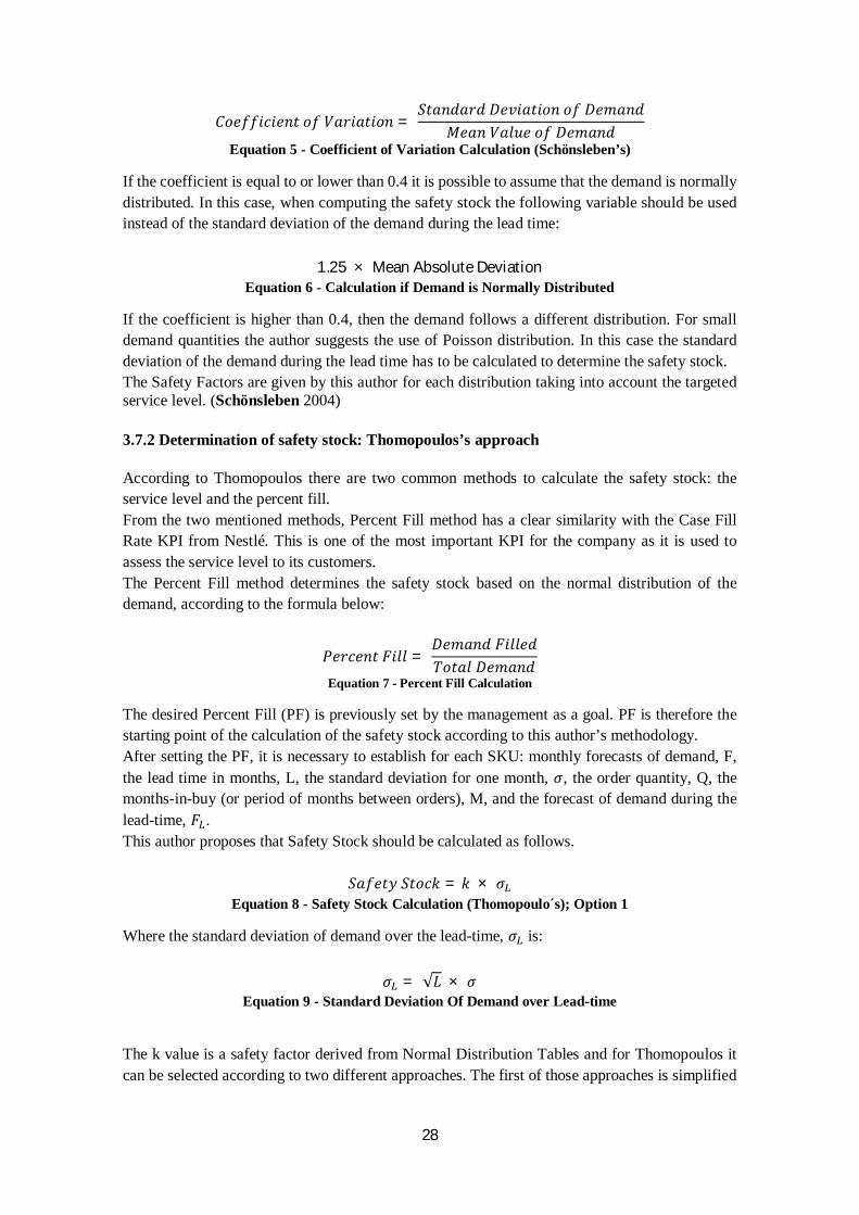
If the coefficient is equal to or lower than 0.4 it is possible to assume that the demand is normally distributed. In this case, when computing the safety stock the following variable should be used instead of the standard deviation of the demand during the lead time:

1.25 × Mean Absolute Deviation Equation 6 - Calculation if Demand is Normally Distributed

If the coefficient is higher than 0.4, then the demand follows a different distribution. For small demand quantities the author suggests the use of Poisson distribution. In this case the standard deviation of the demand during the lead time has to be calculated to determine the safety stock. The Safety Factors are given by this author for each distribution taking into account the targeted service level. (Schönsleben 2004) 3.7.2 Determination of safety stock: Thomopoulos’s approach According to Thomopoulos there are two common methods to calculate the safety stock: the service level and the percent fill. From the two mentioned methods, Percent Fill method has a clear similarity with the Case Fill Rate KPI from Nestlé. This is one of the most important KPI for the company as it is used to assess the service level to its customers. The Percent Fill method determines the safety stock based on the normal distribution of the demand, according to the formula below:

푃푒푟푐푒푛푡 퐹푖푙푙 = 퐷푒푚푎푛푑 퐹푖푙푙푒푑푇표푡푎푙 퐷푒푚푎푛푑

Equation 7 - Percent Fill Calculation

The desired Percent Fill (PF) is previously set by the management as a goal. PF is therefore the starting point of the calculation of the safety stock according to this author’s methodology. After setting the PF, it is necessary to establish for each SKU: monthly forecasts of demand, F, the lead time in months, L, the standard deviation for one month, 휎, the order quantity, Q, the months-in-buy (or period of months between orders), M, and the forecast of demand during the lead-time, 퐹 . This author proposes that Safety Stock should be calculated as follows.

푆푎푓푒푡푦 푆푡표푐푘 = 푘 × 휎 Equation 8 - Safety Stock Calculation (Thomopoulo´s); Option 1

Where the standard deviation of demand over the lead-time, 휎 is:

휎 = √퐿 × 휎 Equation 9 - Standard Deviation Of Demand over Lead-time

The k value is a safety factor derived from Normal Distribution Tables and for Thomopoulos it can be selected according to two different approaches. The first of those approaches is simplified

29

as well as conservative and the other is a bit more complex but should lead to optimized results. The difference relies on the calculation of a parameter called 퐸(푧 > 푘). 퐸(푧 > 푘)휎 is the expected demand exceeding the order point (OP) during the order cycle (OC) and therefore is a measure of the stock that is short during that cycle. It is calculated in the first approach as follows:

퐸(푧 > 푘)휎 = (1 − 푃퐹) × 푄 Equation 10 - Expected Demand exceeding OP during OC

Subsequently, k, the safety factor, can be obtained from Standard Normal Distribution tables using 퐸(푧 > 푘) results derived from the above formula. According to this methodology k should be set to zero for 퐸(푧 > 푘) superior to 0.4, to avoid negative safety stock (the table gives negative values for k), which means no safety stock is needed. The second approach considers the accuracy of the forecast which has direct impact in the computation of the safety stock. The accuracy can be measured with the coefficient of variation, where 휎 is the standard deviation of the one-month ahead forecast error and 퐹 is the average one month forecast.

퐶표푒푓푓푖푐푖푒푛푡 표푓 푉푎푟푖푎푡푖표푛 =휎퐹

Equation 11 - Coefficient of Variation Calculation (Thomopoulo´s)

A low coefficient of variation translates into an accurate forecast, so less safety stock is required. Then 퐸(푧 > 푘) can be calculated as follows:

퐸(푧 > 푘) =(1− 푃퐹) × 푀

√퐿 × 퐶표푒푓푓푖푐푖푒푛푡 표푓 푉푎푟푖푎푡푖표푛

Equation 12 - Expected Demand Calculation

푆푎푓푒푡푦 푆푡표푐푘 = 푘 × 휎 × √퐿

Equation 13 - Safety Stock Calculation (Thomopoulo´s); Option 2

This way the expected demand varies with PF, M, Coefficient of Variation and L. With the k, the Safety Stock, SS, can be calculated. As previously indicated k should be set to zero for 퐸(푧 > 푘) superior to 0.4, to avoid negative safety stock (the table gives negative values for k), which means no safety stock is needed. (Thomopoulos 2015)

30

3.7.3 Determination of safety stock: Chockalingam’s approach The approaches described so far have a common structure: they rely on a safety factor and on a parameter based on past demand. Chockalingam’s method considers the differences between the forecasted demand and the actual demand, i.e. the forecast errors. According to this author the forecast error is the deviation of the actual demand from the forecasted.

퐸푟푟표푟 (%) = |퐴푐푡푢푎푙 − 퐹표푟푒푐푎푠푡|

퐴푐푡푢푎푙

Equation 14 - Forecast Error Calculation

The forecast accuracy evaluates how close the forecasted demand is to reality.

퐴푐푐푢푟푎푐푦 (%) = 1 − 퐸푟푟표푟 (%)

Equation 15 - Forecast Accuracy Calculation

It can be useful to have an Average Error to be able to establish a metric of accuracy through different SKU’s. The Weighted Absolute Percentage Error (WAPE) has the mentioned role.

푊퐴푃퐸 (%) = ∑|퐴푐푡푢푎푙 − 퐹표푟푒푐푎푠푡|

∑퐴푐푡푢푎푙

Equation 16 - Weighted Absolute Percentage Error

So WAPE is the sum all errors, divided by all the actual demand, what gives a good picture about the forecast quality. (Chockalingam 2012) As a side note to Chockalingam (2012) work it should be noted that he suggests that errors should be divided by the actual demand, i.e. what really happened. Nevertheless that is not the practice adopted in Nestlé. An example will help to understand that practice. Consider the expected demand of a product for a certain period of time to be 200 PUM’s, when in reality it corresponded only to 100 PUM’s. According to Chockalingam (2012) this would translate into an error of 100%

퐸푟푟표푟 (%) = |퐴푐푡푢푎푙 − 퐹표푟푒푐푎푠푡|

퐴푐푡푢푎푙=

|100 − 200|100

= 100%

Equation 17 - Forecast Error Calculation in Percentage

So anyone in the company would conclude that the Demand Planner totally failed his forecast, even though the Demand Planner perceived half quantity correctly. In the Nestlé’s perspective the error is calculated in an alternative way that seems more realistic for communicating what has happened (Error Nest).

퐸푟푟표푟 푁푒푠푡(%) = |퐴푐푡푢푎푙 − 퐹표푟푒푐푎푠푡|

퐹표푟푒푐푎푠푡=

|100 − 200|200

= 50%

Equation 18 - Forecast Error Calculation in Percentage for Nestlé

31

This change will lead to a diferent result in Accuracy. In the first situation it will correspond to an accuracy of 0%. In the second situation the accouracy will correspond to 50%, which gives a better approach to evaluate the performance of the predicted demand. (Nestlé 2006) Getting back to Chockalingam (2012) work, WAPE is compared with other different ways to evaluate errors, such as Mean Absolute Error and the Root Mean Squared Error. This author concludes through an example that the best suited indicator is WAPE, due to it is response to different SKU’s and its quantities. In other words, this indicator incorporates the different weight of different products. This author’s perspective on forecast error management, that has been explained so far, is relevant because of its links with Nestlé’s approach that will become relevant at a later stage. With respect specifically to safety stock determination, Chockalingam method requires several variables as indicated below: - The value of the Service Level taken from the Standard Normal Distribution Table. - The Lead Time given in months or weeks, depending on the forecast measuring system. - The Lead Time (the longer the lead time the lower forecast accuracy can be) - The Forecast Error (numerical equal to the Root Mean Squared Error from the formula below).

푅표표푡 푀푒푎푛 푆푞푢푎푟푒푑 퐸푟푟표푟 = ∑( 퐴푐푡푢푎푙 − 퐹표푟푒푐푎푠푡 )

푁

Equation 19 - Root Mean Square Error Calculation

Where N is the number of products included. The Safety Stock can then be calculated (Chockalingam 2012):

푆푎푓푒푡푦 푆푡표푐푘 = 푆푒푟푣푖푐푒 퐿푒푣푒푙 × 퐹표푟푒푐푎푠푡 퐸푟푟표푟 × √퐿푒푎푑 푇푖푚푒

Equation 20 - Safety Stock Calculation (Chockalingam's)

3.8 Addressing the complexity of the case under study with a simple solution (Rojas 2010) The normal distribution should be used when there are uncertainties with respect to the variable under study, like the demand of a product. Indeed, it provides a simple way of modelling the probability density of real life data and recognize patterns. The mean and standard deviation are the only required parameters to establish a one-dimensional normal distribution. As a rule of thumb, in cases where there is no clear idea how does the specific probability distribution behave, using the normal distribution is the safe option. (Rojas 2010)

3.9 Industry sources The survey of literature included not just the academia, but also the industry like for instance in Systems, Application & Products in Data Processing (SAP). Nestlé is a customer of SAP, which is a corporation that makes enterprise software to manage issues such as business operations.

32

A reference was found, Supply Chain Management with APO, from Dickersbach (2008) about how to implement one of SAP offered solutions related to stocks. It includes a section called “Stock and Safety Stock”. However the only relevant fact mentioned is that Safety Stock is dealt as a demand element and not a stock category in order to have an earliness of the supply. In spite of its interest for SAP, it is does not add anything relevant to this study.

3.10 Conclusions of the State of the Art 3.10.1 Introduction As previously mentioned investigating the State of the Art faced several difficulties, related to the proprietary nature of the “Optimizer Tool” (therefore not mentioned in the literature) and to the specificities of the situation under study with respect to stock optimization. To further illustrate these specificities of the situation, it should be underlined that stock optimization may have different perspectives inside a complex organization. From a strict engineering perspective it seems enough that the SKU’s available on a shelf are the SKU’s that are being requested by final consumers. However if final consumer behavior is considered, then stock optimization includes keeping a certain length of shelves filled with Nestlé’s SKU’s and filling constantly any empty space on those shelves. That made necessary a careful selection of the literature, to avoid what could be inapplicable, and the review was then made to understand the current knowledge on the subject under study. 3.10.2 Summary of literature review The main issues that emerged from literature review were:

- The importance of methodologies to prioritize SKU’s according to relevant criteria, called Classification Schemes; optimization efforts should then be concentrated on the SKU’s with highest rate.

- Unless there is an adequate quantity of updated and reliable information enabling proper forecast of demand, the application of the normal distribution is a simple and cost-effective method that delivers acceptable results.

- Besides the uncertainty of demand, there are also uncertainties in the whole production and supply network that increase with the complexity and size of the company. If all of those uncertainties are not easy to control, then a planning approach based on the rolling horizon framework methodology (basically learn as you go process) is recommended.

- The safety stock is in any case an important concept and several methodologies were found in the literature.

The review of literature confirmed that DSP operates according to what was found to be the state of the art. 3.10.3 Using the literature review to define the next steps The most relevant conclusions that can be derived with impact on the next steps are:

- Classification schemes are very important to allow inventory control to be concentrated on those SKU´s that matter the most to the company. In line with Nestlé’s option ABC classification will be used in the subsequent phases of this thesis.

33

- Different classification schemes can be combined according to SAW methodology thus allowing an improved result based on the complementarity of the schemes. As Nestlé does not use SAW this thesis will include a practical application to explore its potential to contribute for the objectives of this study as well as to answer the research question.

- In line with the paper identified in the survey that recommends the use of the normal distribution in complex (and ever changing) environments, Nestlé uses the normal distribution to forecast demand. That approach will be kept in the future steps of the work.

- After selecting the most important SKU’s, there is always the need to deal with the uncertainties of the respective demand, as well of the production and supply network. Therefore a planning approach based on the rolling horizon framework methodology, that basically corresponds to what Nestlé is already doing, will be used.

- Moreover other company policies present limits to other theoretical approaches, namely in respect to inventory management. For the company, a lost sale risks to be a lost client and therefore a problem in terms of market share. So Nestlé is willing to work in sub optimum conditions to prevent the hidden cost of a lost sale.

- The different methodologies described in the literature for determination of safety stock have their range of application. During the next phases of the work those methodologies will be considered in relation to Nestlé’s options for safety stock determination if applicability becomes clear.

3.10.4 Closing remarks of the state of the art The contributions of literature review to the next steps of the work will support a methodology of study of a proprietary system (“Optimizer Tool”) to investigate its possibilities of improvement. This work presents a challenge that, according to this state of the art, has not yet been developed.

34

4. Methodology Recalling that stock policies are a product of an interaction of the “Optimizer Tool” with human judgement, the research question formulated in section 1.5 was: How to optimize the integration of “Optimizer Tool” operation with the inherent human judgement? In the same section the following two hypothesis were formulated: H1: There is no detectable problem in “Optimizer Tool” operation that recommends a specific reformulation of any of its modules. H2: The variables that the Supply Planner is allowed to adjust have great influence on the “Optimizer Tool” final results. Therefore the first step will be to test and validate those hypothesis, what is presented in section 6.1 for H1 and in section 6.3 for H2. Subsequently the methodology of the work can be separated into two phases, which will deliver what is required to meet the requirements of DSP (as defined in section 1.5) as well as to answer the research question. In the first phase, a complement (add-on) to the “Optimizer Tool” will be implemented, based on the results from the literature review, like the SAW methodology and the rolling horizon framework. In the second phase, a case study of the “Optimizer Tool”, focused on a set of SKU’s from the Cereals category (as indicated in section 1.6), will be made using the add-on for demonstration purposes. In the next section a conceptual description of the “Optimizer Tool” will be provided, for a better understanding of the subsequent parts of the work and also to show the complexity of the system, that prevents other approaches.

35

5. The “Optimizer Tool”

5.1 Description of operation The “Optimizer Tool” uses historical data from the previous year and from the approved plans for the next year to support the decision making process in relation to stock policies: finished goods minimum and maximum stock cover levels (expressed in days). (Nguyen 2014) This section briefly illustrates the calculation process, the interaction with the user, the integration with other information available in the company and the outputs (numerical and graphical outputs). For that purpose, the following scheme sumarizes the main steps of a “Optimizer Tool” run and what is done at each one. The numbers refer to the text where further explanation will be provided.

Figure 11 - “Optimizer Tool” Scheme of Operation

Step 1 – At this stage the supply planner that is using the “Optimizer Tool” indicates a category of SKU’s, the source (e.g., factory) the SKU’s are coming from and the distribution center where they will be delivered. As already indicated the tool has been developed for Mono-Echelon networks (distribution networks with a single distribution center). Step 2 – The tool automatically retrieves the most relevant information regarding the last 12 months in terms of demand, production, etc. pertaining to each SKU of the defined category that came from the specified source. Afterwards the “Optimizer Tool” looks for the projections made available by the Demand Planner in terms of requirements of each SKU for the incoming 12 months. Step 3 – The Supply Planner completes the inputs needed by the tool according to the list below for each SKU.

A. Demand Details a. CFR target: the default value for Nestlé is 99%; b. Adjusted DPA: Adjustments can be made to the results of automatic information

retrieval according to how well predictions have worked in the past for a particular SKU. The Supply Planner should decide in coordination with the Demand Planner the cases where a more optimistic or pessimistic value can/has to be adopted.

36

B. Distribution Details a. Frozen Horizon Dispatches: Represents the number of days during which the

load plan cannot be changed, for example those needed to get the customs necessary documents.

b. Constrained Delivery Frequency: estimated delivery frequency between source and distribution center; for example once per week.

c. Minimum Transit Time: the minimum number of days for transportation time. d. Maximum Transit Time: the maximum number of days for the transportation

time. C. Technical & Production Details

a. Production Stability Period: number of days during which the production plan cannot be changed (occasionally there may be exceptions but they are not considered for this purpose).

b. Minimum Lot Size: minimum production in terms of PUM (packages of a particular SKU).

c. Quality Assurance (QA) Release time: number of days necessary to perform quality assurance.

d. Early Shipment: maximum number of days for a set of SKU’s to be allowed to be shipped from source to distribution center when the results of the quality assurance are not known.

e. Adjusted MSA: Adjustments can be made to the results of automatic information retrieval according to how well production has met the agreed quantities in the past for a particular SKU. The Supply Planner should decide in coordination with the Detailed Production Scheduling of the factory which cases a more optimistic or pessimistic value can/has to be adopted.

D. FreshNes (Freshness Nestlé) a. Total shelf life: Number of days the product lasts until it can no longer be

consumed. b. Minimum Required Customer: Minimum number of days of total shelf life at

which the customer is still willing to buy the product (normally 66% of the total shelf life).

Step 4 – The “Optimizer Tool” interacts with the user proposing a minimum stock cover level for each SKU. At this stage that minimum stock cover has to be approved or modified by the user. In the latter case a new maximum stock cover will be calculated. (Macca 2012) Step 5 – Finally the stock policies are defined in relation to each SKU (pertaining to the category and source indicated at step 1) for the next 3 to 4 months period. In reality, the calculated stock policies for each SKU will have to be validated by the respective source (i.e. the factory) before being adopted, as CFR is a common objective. Indeed, if decisions taken along the above described process rely on the responsibility of the Supply Planner, the match between orders received and orders delivered (CFR) is a shared responsibility. After that validation the Supply Planner implements the stock policies, using other available information management tools. It is important to underline for the sake of clarity that the stock policies are not a direct output of the “Optimizer Tool”. What comes out directly from the system is the minimum stock cover level.

37

This parameter, once approved, is used to calculate the maximum cover level from what results a complete definition of a stock policy.

5.2 How inputs of the “Optimizer Tool” impact stock policies This section is intended to highlight the relationship between the most relevant inputs that are used by the “Optimizer Tool” and the impact on stock policies (minimum and maximum stock cover levels):

1. CFR (Case Fill Rate) reveals how well customers’ needs are being met and has a default value of 99%. Any change of this target requires a company decision as it implies possible loss of market share. Possible values range from 85 to 100%. A smaller CFR has a decreasing effect on stock cover levels.

2. DPA M-1 is automatically retrieved by the system and translates the past accuracy of demand forecast. An increase of uncertainty leads to higher stock cover levels, to achieve a pre-determined CFR.

3. Adjusted DPA allows the Supply Planner to override the automatically calculated DPA value, thus introducing a correction factor.

4. MSA is automatically retrieved by the system and refers how production has met the agreed quantities on a weekly basis. The lower the MSA the higher the stock cover levels.

5. Adjusted MSA allows the Supply Planner to override the automatically calculated MSA, thus introducing a correction factor.

6. Production Stability Period represents the number of days during which an order cannot be changed. A smaller production stability period means higher production flexibility and reduced stock cover levels.

7. QA Release Time refers to quality assurance tests. Therefore a higher QA Release time has an increasing effect on stock cover levels.

8. Minimum Lot Size is also a measure of production flexibility. Therefore the decrease on lot size has a decreasing effect on stock cover levels.

9. Minimum and Maximum Transit Time a parameter that has a greater impact on stock cover levels as distances increases. Therefore, they are more important when products are imported.

From the above explanation it becomes clear that the Supply Planner has not much degree of freedom to change input 1 because it is a company objective. In most cases inputs 6 to 9 have stationary values in routine operations. The obvious conclusion is the importance of inputs 2 to 5 for “Optimizer Tool” output. This conclusion will be further developed in the next sections of the research work.

38

6. Analysis of the problem and proposals

6.1 Hypothesis 1 test and validation. Development of insight into how to improve the “Optimizer Tool” Considering the context of the problem that motivated Nestlé in this work as described in sections 1.3 and 1.4, as well as the objectives indicated in section 1.5, a comprehensive interaction with the “Optimizer Tool” was undertaken to investigate its operation, behavior and specificities. This phase took a considerable amount of time that can be estimated as close to 30 days of full time work. During that work with the “Optimizer Tool” with an extensive set of real life data from Nestlé’s historical records, no symptoms of lack of soundness on results, instability or ineffectiveness was detected. Consequently it can be assumed that Hypothesis 1 is valid. On the other hand, it was confirmed that an analytical approach to the problem is out of the scope of this thesis work, not only because of confidentiality issues, but also because of the inherent complexity of the tool as a result of years of experience, linking theory with practice. Such context would make that approach incompatible with the available timeframe. Therefore, an empirical approach has to be adopted as the way to address the problem. Besides validation of Hypothesis 1, other important conclusions were drawn as explained subsequently. A first conclusion is that, if the empirical approach is adopted, there is no reason to develop a dedicated activity to improve analytically the determination of safety stock (the possibility of studying alternative ways to determine safety stock was addressed in section 3.10.3). This is the main component of minimum stock cover level and therefore safety stock improvement is implicit in achieving the thesis’s goals. A second conclusion is that the output of a run of “Optimizer Tool” establishes stock policies for a significant period of time where the respective assumptions change considerably. In fact many unforeseen factors can have relevant impact on demand, like for instance a big supermarket chain that suddenly decides to offer rebates on a set of SKU’s or an opportunity that is spotted by Nestlé to increase sales because of unexpected market conditions for some SKU’s. A third conclusion is that the “Optimizer Tool” operators have relevant empirical knowledge on how to manage that uncertainty, enabling them to contribute to the adjustment of the calculations regarding stock policies. This is taken into account as described in section 5 also with the inputs operators get from Demand Planners and from Detailed Production Scheduling. But such adjustments are presently made only with subjective knowledge from the person that is there at the moment. A fourth and last conclusion is that the “Optimizer Tool” calculations do not incorporate the relative importance of some SKU’s for the company turnover and/or company strategy for a particular market (i.e., classification schemes as described in sections 3.6 and 3.10 are not considered in the tool). In other words, the two last conclusions can be summarized as follows: i) that the “Optimizer Tool” treats equally what is indeed different; ii) it is up to the Supply Planner to do his or her best to overcome that situation; iii) presently that is being done with subjective and informal decisions, adjusting inputs as referred in the last paragraph of section 5.2.

39

6.2 What the insight has revealed to guide the next research steps The two last conclusions from section 6.1 underline the importance of the research question and, taking in consideration the results of the literature review, suggest two possible improvements to investigate (what is aligned with section 3.10.3):

- Complementing the “Optimizer Tool” with a layer of calculation that allows introducing differences among SKU’s according to criteria like for instance contribution for turnover and company strategy.

- Providing the “Optimizer Tool” operator with some kind of decision support system that may complement his or her experience.

But the latter improvement is useful only if Hypothesis 2 is validated: the quality of the decisions of the “Optimizer Tool” operator has great impact on the adopted stock policies. The test and validation will be done with a sensitivity analysis which will not aim at establishing a function of how one variable varies with another variable (quantitative analysis). Rather the objective is to verify if the inputs of the tool that are more subject to uncertainty (market variations or production ups and downs) and that the operator can adjust are the most sensitive for “Optimizer Tool” results (qualitative analysis).

6.3 Hypothesis 2 test and validation: Sensitivity Analysis

6.3.1 SKU selection for sensitivity analysis As mentioned in section 3.10.2 classification schemes are differentiation methodologies that the reviewed literature indicates as valid to support prioritization of SKU’s according to relevant criteria, like turnover or market strategy. Therefore in section 3.10.3 it is mentioned that classification schemes allow inventory control to be concentrated to those SKU´s that matter the most to the company. In line with Nestlé’s option, ABC classification will be used in the present context. The ABC classification for SKU’s can be retrieved directly from the “Optimizer Tool” according to contribution for turnover. That will allow more accurate interpretation of the results of the sensitivity analysis. As a result of the application of this and other criteria, four different SKU’s from Cereal’s category (the main focus of the analysis by the reasons indicated in sections 1.6 and 4) will be considered to carry out the study case:

- SKU W classified as A - SKU X classified as B - SKU Y classified as C - SKU Z classified as A and produced abroad

This selection of SKU among the Cereals category was developed to have a representative of each class (A, B and C). That group of 3 SKU’s was completed with another that has a distinctive characteristic: it is not produced in Portugal. The importance of those SKU’s is illustrated as follows;

- SKU W has a projected average demand of 8.596 PUM5 per week. Overstock and understock situations occurred recently, revealing difficulties of forecast, and therefore

5 A PUM is a package of SKU (items with same product identification number) for logistic purposes. A PUM of a particular SKU has always the same number of items.

40

DPA is low (70%). The respective minimum lot size of production is 10.000 PUM, equivalent to about 8,1 days of stock cover at projected average demand levels.

- SKU X has a projected average demand of 982 PUM per week. The respective minimum lot size of production is 3.300 PUM, equivalent to 23,5 days of stock cover at projected average demand levels.

- SKU Y has a projected average demand of 801 PUM per week. The respective minimum lot size of production is 3.300 PUM, equivalent to 28,8 days of stock cover at projected average demand levels.

- SKU Z, produced in La Penilla, Spain, has a projected average demand of 1.288 PUM per week. The respective minimum lot size of production is 2.000 PUM, equivalent to 10,9 days of stock cover at projected average demand levels.

For the selected the SKU’s it is worthwhile to indicate a representative example of the “Optimizer Tool” outputs and the minimum stock cover levels that are in fact implemented by the Supply Planners:

Table 3 - Examples of outputs from “Optimizer Tool” and Supply Planners’ decision regarding minimum stock cover level

The above examples illustrate the importance and relevance of the approach for the next steps of the thesis work as suggested in section 6.2.

6.3.2 Sensitivity analysis

As referred above a sensitivity analysis in respect to stock policies determination will be made for the SKU’s selected in the previous section, using historical data of inputs from Supply Planners (for each of the variables indicated in step 3 of section 5). In other words, the variations will be applied to each variable the Supply Planners use, while keeping all others constant. Also as mentioned in section 6.2 the sensitivity analysis will aim at a qualitative analysis. Its only purpose is to confirm that those inputs more subject to uncertainty (market variations or production ups and downs), and that the operator can adjust according to his or her criteria, are the most sensitive for “Optimizer Tool” output. The detailed results of the sensitivity analysis are presented in Appendix I. The most relevant issues are summarized in the figures below.

SKU W 18,3 8

SKU X 14,9 10

SKU Y 19,4 11

SKU Z 13,4 12

SKU"Optimizer Tool" Min. Stock Cover

Level

Current Min. Stock Cover

Level

41

Figure 12 - Results of sensitivity analysis of “Optimizer Tool” output with 25% decrease on inputs

Figure 13- Results of sensitivity analysis of “Optimizer Tool” output with 25% increase on inputs

As CFR (related to quality of service) is an absolute company target, and therefore it is not really a variable, it was not considered in the analysis. To understand Figure 13, it must be noted that MSA (as well as the adjusted MSA) has typically a high value and consequently a 25% increase would lead to more than 100%. Therefore it was not included in that part of the sensitivity analysis. Anyway, this situation does not affect the conclusions. From the results obtained, it becomes clear that the variables with greatest impact on the final result of the “Optimizer Tool” (in terms of stock policies) will be the Adjusted DPA (accuracy of demand projections for a category of SKU’s) and the Adjusted MSA (how well a production facility meets the goals of manufacturing the agreed quantities). Those variables are just the result of DPA M-1 and MSA, after being adjusted by the “Optimizer Tool” operator as described in section 5.

42

6.3.3 Conclusions of the sensitivity analysis

Considering the results from section 6.3.2, it can be stated that Hypothesis 2 is valid. It is possible then to state that the “Optimizer Tool” calculations are extremely sensitive to variables that incorporate uncertainties from the production and demand levels, precisely the variables that the operator is supposed to adjust according to his or her experience. Therefore from the vast list of inputs listed in section 5.1, it is clear that the top three in terms of impact on stock policies (and consequently on safety stock) are: CFR, DPA M-1 and MSA. As CFR is a company target, in fact all comes to DPA M-1 and MSA (or the respective adjusted values). Not surprisingly, Nestlé has been investing in improving those parameters, in the first case based on information management systems and in the second case making production more efficient and reliable. These conclusions indicate how the research question can be answered and underpin the likelihood of improving the “Optimizer Tool” results with a reinforcement of the “human factor”, complementing informal knowledge and experience with some kind of decision support system.

6.4 Using classification schemes for the decision support system: answering the research question As referred in sections 3.6 and 3.10 classification schemes can assist in SKU management according to objective and relevant criteria. Additionally classification schemes are easy to introduce, operate and can be updated with not much effort to reflect new conditions or the accumulated experience. So, as already mentioned in sections 6.1 and 6.2, this opens an opportunity that has to be investigated to deliver what is required by DSP and to answer the research question. Just incidentally the “Optimizer Tool”, generates a classification of SKU’s according to ABC scheme6, but does not make use of them for stock cover levels purposes. That was already mentioned in section 6.2.1, where a decision support system to complement the adjustment of DPA M-1 and MSA done by Supply Planners when using the “Optimizer Tool” was also referred. It seems obvious that the two improvements opportunities identified in section 6.2 can be combined into just one tool, referred to as an add-on. As a matter of fact, classification schemes are suitable to incorporate human experience and knowledge and therefore can be used and updated in respect to support decisions when making adjustments of the “Optimizer Tool” outputs. For the intermediate inputs, Adjusted DPA and Adjusted MSA, Nestlé has target values that can be used. Such target values exclude the option of applying classification schemes at that level.

6 Just for informative purposes.

43

6.5 Add-On Development: Classification Schemes and application of their results 6.5.1 Classification Schemes

As referred in section 3.10.3 that described how literature review was defining the next steps: “After selecting the most important SKU’s, there is always the need to deal with the uncertainties of the respective demand, as well of the production and supply network. Therefore a planning approach based on the rolling horizon framework methodology (…) will be used”. Recalling (Minner 2000) definition, the rolling horizon framework requires forecasts about the future as a kick off for decisions regarding planning, followed by interactive cycles on subsequent periods. Every cycle comes with forecasts updates and re-planning actions. That is precisely what will be done at this stage. On the other hand, it was mentioned in the same section: “Different classification schemes can be combined according to SAW methodology thus allowing an improved result based on the complementarity of the schemes. As Nestlé does not use SAW this thesis will include a practical application to explore its potential to contribute for the objectives of this study as well as to answer the research question.” For that purpose the practical experience of using the “Optimizer Tool” was used by the author of this thesis work to develop a set of classification schemes tailored to the needs of a Supply Planner, as they incorporate the several sources uncertainty of DPA M-1 (unexpected promotions, new marketing strategies, market trends, etc.), as well as information available on MSA and on noncompliance of the target for CFR. Those classification schemes complement the already known ABC classification as well as the Animal Farm classification already in use at Nestlé. The table below summarize and describe the classification schemes including those classification schemes developed for this purpose by the author of this thesis work (Positive Bias, SKU’s frequency of sales promotion, SKU Business Bet, MSA, Pareto analysis based on PUM’s and OOS).

44

Table 4 - Classification Schemes to use in the add-on

Classification Scheme Criteria for classification

Animal Farm

Relation / Motivation Classes / Points

DPA M-1 / Business as usual

Volatility (of demand)- low volatility means stability of demand- high volatility means unpredictibility of demandProfitability (contribution to turnover)

Mad Bulls: 3 (high volatility and significant profitability)Horses: 2 (low volatility and significant profitability)Jack Rabbits: 1 (high volatility and non-significant profitability)Mules: 0 (low volatility and non-significant profitability)

Positive Bias

Occurrence of DPA M-1 problems consisting on frequent overforecasting. Overforecasting means higher than needed minimum stock cover level and/or sales below the expectations.

DPA M-1 / Early identification of possible trends

0 to 1 month of positive bias in one year corresponds to 3 points2 months of positive bias in one year corresponds to 2 points3 months of positive bias in one year corresponds to 1 pointmore than 3 months of positive bias in one year correspond to 0 points

SKU's frequency of

sales promotion

(1)

Achievement of sales objectives on a category of SKU's may sometimes require promotions of those SKU (of the category) that are most profitable. This is quite unpredictable and may lead to Out of Stock situations unless the Supply Planner provides a "just in case" component in the minimum stock cover level.

A SKU with high frequency of sales promotion is classified with 3 pointsA SKU with medium frequency of sales promotion is classified with 2 points A SKU with low frequency of sales promotion is classified with 0 points

3: 92% corresponds to company target. 87% corresponds to the historical worst case scenario.

Out of Stock (OOS)

Accumulated number of PUM's not delivered over one year due to a Nestlé Failure that translates into an Out of Stock situation (related to CFR). This allows the Supply Planner to perceive failures in defining minimum stock cover levels in the past.

CFR / OOS means sales loss and

moreover a potential reduction in market

share

0 to 100 accumulated PUM's not delivered over one year corresponds to 0 points101 to 500 accumulated PUM's not delivered over one year corresponds to 1 point501 to 1000 accumulated PUM's not delivered over one year corresponds to 2 pointsMore than 1000 accumulated PUM's not delivered over one year corresponds to 3 points

ABCContribution to turnover. The Supply Planner will increase minimum stock cover levels of a SKU of A class in relation to a SKU of class C.

TurnoverA class corresponds to 3 pointsB class corresponds to 2 points C class corresponds to 1 point

MSA

DPA M-1 / Additional stock

cover level to account for promotions

DPA M-1 / Additional stock

cover level to account for new marketing

strategies

1: To be determined with the Demand Planner of a category and should be attributed comparing each SKU to other SKU's of that category

2: To be determined comparing each SKU to other SKU's of that category

Business SKU Bet

(2)

Every year the marketing team of each category decides which SKUs are the ones to bet on, based on market trends and profitability. Frequently bets fall on SKU's of B or C (from ABC classification) that the marketing team believes have potential to grow to the next class (A or B respectively).

A big bet on a SKU should be classified with 3 points Other SKU's with good position within the market or a good growth rate are classified with 2 points The SKU's that have a declining position and/or are considered to be descontinued should be classified with 1 point

Master Schedule Attribute

(MSA)

Reliability of a factory in delivering the agreed quantities on time. Based on historical data, the Supply Planner can make decisions on minimum stock cover levels.

92% or more of MSA in a SKU corresponds to 1 pointless than to 92% but above 87% of MSA in a SKU corresponds to 2 pointsbelow 87% of MSA in a SKU corresponds to 3 points

Pareto Analysis based on PUM's

Contribution to storage costs. As the amount of PUM’s of a SKU from a category (expressed as percentage of the total PUM’s of that category) increases, the more capacity, namely in terms of storage, has to be allocated to that SKU through the supply chain. This represents a cost that needs to be considered, together with uncertainties.In other words, overcoming high uncertainties may come at a relevant cost and that effect has to be considered as a counterbalance in SAW methodology.

Storage Costs

A SKU responsible for more than 15% of PUM's of its category corresponds to 0 pointsA SKU responsible for more than 10% to 15% of PUM's of its category corresponds to 1 pointA SKU responsible for more than 5% to 10% of PUM's of its category corresponds to 2 points A SKU responsible for less than or equal to 5% of PUM's of its category corresponds to 3 points

45

The above classification schemes, which incorporate several uncertainty factors with impact on “Optimizer Tool” results (except for ABC and Pareto Analysis respectively based on turnover and on PUM’s), will be combined following the SAW methodology as explained at a later stage to support better decisions in respect to stock policies. For the moment it is important to underline that for each classification scheme the higher the number of points, the greater a minimum stock cover level has to be (or can be in the case of Pareto Analysis). And, inversely, the lower the number of points, the smaller a minimum stock cover level has to be. It should also be noted that Animal Farm classification scheme is used by Nestlé for Demand Planners. Considering the importance of DPA M-1 for "Optimizer Tool" output, this classification will also be used for Supply Planners' scope of work. 6.5.2 Application of classification schemes: SAW methodology

The table below summarizes criteria for attribution of points.

Table 5 - Criteria for attribution of points on each classification scheme

The application of the SAW methodology (refer to section 3.6) implies that each classification scheme is given a percentage weight. For the present thesis work three possibilities will be considered as show in table below.

Table 6 - Suggestions of percentage weights for SAW methodology

The rationale of the suggestions corresponds to a stepwise approach of increasing complexity: - Suggestion 1: This is most straightforward approach. It combines on equal proportions

unpredictability of demand (DPA M-1) and noncompliance of CFR, attributing the remaining weight to production reliability (MSA).

3 Points 2 Points 1 Point 0 Points

Animal Farm Mad Bull Horses Jack Rabbit Mule

Positive Bias (in a 1 year period)

0 – 1 Month 2 Months 3 Months More than 3 Months

SKU frequency of sales promotion

High frequency Medium frequency Low frequency -

Business SKU Bet A bet to excel in the market Good market but no bet Not so good in the market -

MSA Less than 87 % 87 % to 92 % More than 92% -

OOS (in a 1 year period)

More than 1000 PUM's 501 to 1000 PUM's 101 to 500 PUM's 0 to 100 PUM's

ABC A B C -

Pareto Analysis based on PUM's

Less or equal to 5% of PUM's of its category

More than 5% to 10% of PUM's of its category

More than 10% to 15% of PUM's of its category

More than 15% of PUM's of its category

Suggestion 1 40,0% - - - 20,0% 40,0% - -

Suggestion 2 20,0% 20,0% - - 20,0% 20,0% 20,0% -

Suggestion 3 20,0% 10,0% 10,0% 10,0% 10,0% 20,0% 10,0% 10,0%

Pareto Analysis based

on PUM'sMSA OOS ABC

Animal Farm

Positive Bias

SKU frequency of sales promotion

Business SKU Bet

46

- Suggestion 2: In relation to the previous situation two additional indicators are introduced. The first is related to early identification of market trends and the other to turnover. As the weights are equally distributed that means a relatively higher importance of DPA M-1 (related to Animal Farm and Positive Bias).

- Suggestion 3: In this case the impact of marketing options and of storage costs are also taken into account, with a transfer of weight to the respective classifications schemes from all others except those more directly linked to DPA M-1 (Animal Farm) and CFR (OOS).

In any event the sum of weights given to DPA-related classification schemes (Animal Farm, Positive Bias, SKU frequency of sales promotion and Business SKU Bet) with the weight given to MSA-related classification scheme is always equal to or higher than 60%, which is in line with the importance of those parameters to “Optimizer Tool” results as demonstrated by the sensitivity analysis. 6.5.3 Adaptation of SAW methodology to the SKU’s under study

In the previous section the scale of points was defined regardless of any specific situation. It was a mere conceptual definition of what each point of a classification scheme means. However, when specific SKU’s are considered, the attribution of points has to consider its past history. More than just a theoretical requirement, this is a first step to put classification schemes at work for the purpose of supporting the right decisions. The table below summarizes the points that each SKU can be given in relation to each classification scheme on the basis of its past history.

Table 7 - Points of each SKU in relation to classification schemes based on past data methodology

Applying the maximum of points of the table above to the weights of each suggestion presented in section 6.5.2 the result is as follows:

Table 8 - Application of maximum points of each classification scheme to the suggested weights

At this point it is very important to explain the meaning of the total obtained for each of the above suggestions. For that purpose let’s recall what was done:

SKU W 3 0 3 3 2 0 3 2

SKU X 2 0 2 2 1 1 2 2

SKU Y 1 0 2 3 1 0 1 2

SKU Z 2 2 1 2 3 0 3 3

Pareto Analysis based on PUM'sMSA OOS ABCAnimal

FarmPositive

BiasSKU frequency of sales promotion

Business SKU Bet

Suggestion 1 1,20 - - - 0,60 0,40 - - 2,20

Suggestion 2 0,60 0,60 - - 0,60 0,20 0,60 - 2,60

Suggestion 3 0,60 0,20 0,30 0,30 0,30 0,20 0,30 0,30 2,50

MSA OOS ABC Total Animal Farm

Positive Bias

SKU frequency of sales promotion

Business SKU Bet

Pareto Analysis based on PUM's

47

- The starting point was the maximum number of points for each classification scheme obtained in the past by a set of SKU of the same category (not by a particular SKU of the category).

- That maximum number of points for each classification scheme is related to the highest degree of safety in terms of minimum stock cover levels according to historical data (except for Pareto Analysis based on PUM’s which is related to storage costs). That degree of safety can be either directly reflected in the classification scheme or indirectly reflected (as will be the case of ABC that is really a function of turnover that is somewhat linked to demand).

- Applying those maximums to the weights of each suggestion and summing up each component, a total is obtained.

- Each total obtained is related to the highest degree of safety in terms of minimum stock cover levels according to historical data after balancing various factors that contribute to the uncertainty (with Pareto Analysis based on PUM’s acting as counterforce proportional to storage costs).

6.5.4 Application of SAW methodology to the SKU’s under study

The above methodology was applied to each SKU under study. Each of the values of the tables below were calculated using the individual values from table 7 that were multiplied by the weight factors indicated in table 6.

Table 9 - Application of SKU W points of each classification scheme to the suggested weights

Table 10 - Application of SKU X points of each classification scheme to the suggested weights

Table 11 - Application of SKU Y points of each classification scheme to the suggested weights

Suggestion 1 1,20 - - - 0,40 0,00 - - 1,60Suggestion 2 0,60 0,00 - - 0,40 0,00 0,60 - 1,60Suggestion 3 0,60 0,00 0,30 0,30 0,20 0,00 0,30 0,20 1,90

TotalSKU W MSA OOSAnimal Farm

Positive Bias

SKU frequency of sales promotion

Business SKU Bet

Pareto Analysis based on PUM's

ABC

Suggestion 1 0,80 - - - 0,20 0,40 - - 1,40Suggestion 2 0,40 0,00 - - 0,20 0,20 0,40 - 1,20Suggestion 3 0,40 0,00 0,20 0,20 0,10 0,20 0,20 0,20 1,50

MSA OOS ABC TotalSKU X SKU frequency of sales promotion

Business SKU Bet

Animal Farm

Positive Bias

Pareto Analysis based on PUM's

Suggestion 1 0,40 - - - 0,20 0,00 - - 0,60Suggestion 2 0,20 0,00 - - 0,20 0,00 0,20 - 0,60Suggestion 3 0,20 0,00 0,20 0,30 0,10 0,00 0,10 0,20 1,10

Animal Farm

Positive Bias TotalSKU Y MSA OOSSKU frequency of

sales promotion Business SKU Bet

Pareto Analysis based on PUM's

ABC

48

Table 12 - Application of SKU Z points of each classification scheme to the suggested weights

The explanation of the meaning of the totals obtained given in the previous section applies here as well. However in these cases the maximum value obtained by the set of SKU’s of the same category at each classification scheme was not used. What was used here was the value attributed to each of those schemes by a particular SKU. That value was then multiplied by the weights included in the suggestions and the components summed up to give a total. Each total obtained is therefore related to the highest degree of safety in terms of minimum stock cover levels of a particular SKU according to historical data after balancing various factors that contribute to the uncertainty. A more practical way to represent the totals obtained in tables 9 to 12, related to each SKU, is to calculate what they represent in percentage of the total obtained in table 8, related to the maximum value that the set of SKU’s under study can get. That is presented in table below.

Table 13 - Balanced classification for each SKU (SAW methodology) expressed as percentage of the

maximum classification for three suggestions of weighting

Suggestion 1 0,80 - - - 0,60 0,00 - - 1,40Suggestion 2 0,40 0,40 - - 0,60 0,00 0,60 - 2,00Suggestion 3 0,40 0,20 0,10 0,20 0,30 0,00 0,30 0,30 1,80

SKU frequency of sales promotion

Business SKU Bet

SKU Z Animal Farm

Positive Bias

MSA OOS ABC TotalPareto Analysis based on PUM's

Results in % Suggestion 1 Suggestion 2 Suggestion 3

SKU W 57% 62% 76%

SKU X 50% 46% 60%

SKU Y 21% 23% 44%

SKU Z 50% 77% 72%

49

6.5.5 “Optimizer Tool” add-on: conceptual explanation and application

It was an initial assumption that the “Optimizer Tool” overestimates the minimum stock cover levels (the size of the problem was illustrated in table 3). During the thesis work it was possible to demonstrate that a part of the problem arises from DPA M-1 and MSA or their adjusted values. It also became clear that the adjustment process, which takes place every time the “Optimizer Tool” is used is subjective and informal. Consequently, the material collected from the literature review is now being used to answer the research question, support better decisions in adjustments (not of intermediate inputs, but of final results) and to create a framework where the accumulated experience by Supply Planners can be shared and used according to a standardized procedure. That is what was called the add-on to the “Optimizer Tool”. At this stage the use of the add-on will be demonstrated using the data from table 6 and from table 7. For that purpose, as it is known that the “Optimizer Tool” overestimates the minimum stock cover levels, each of its results for the set of SKU’s under study will be assumed to be in line with the corresponding maximum values obtained from SAW methodology as explained in section 6.5.3. For a start this assumption is quite reasonable. Therefore, the adjusted results of “Optimizer Tool” will be obtained applying to the initially calculated minimum stock cover levels the percentages indicated in table 13. The tables below show the application of the add-on and compare the results with current minimum stock cover levels (Supply Planners decisions). The two tables differ because in one case the adjusted DPA and the adjusted MSA was based on historical values and in the other case the adjustment was based on company target values. The detailed calculations are explained in Appendix II. Table 14 - Application of add-on to “Optimizer Tool” using historical values for adjusted DPA and

adjusted MSA

Table 15 - Application of add-on to “Optimizer Tool” using target values for adjusted DPA and

adjusted MSA

SKU W 18,3 10 Days 11 Days 14 Days 8

SKU X 14,9 7 Days 7 Days 9 Days 10

SKU Y 19,4 4 Days 5 Days 9 Days 11

SKU Z 13,4 7 Days 10 Days 10 Days 12

"Optimizer Tool" Min. Stock Cover

Level

Current Min. Stock Cover

LevelSuggestion 1 Suggestion 2 Suggestion 3

SKU W 13,9 8 Days 9 Days 11 Days 8

SKU X 15,7 8 Days 7 Days 9 Days 10

SKU Y 15,4 3 Days 4 Days 7 Days 11

SKU Z 15,3 8 Days 12 Days 11 Days 12

Suggestion 2 Suggestion 3"Optimizer Tool" Min. Stock Cover

Level

Current Min. Stock

CoverLevelSuggestion 1

50

7. Conclusions and discussion

7.1 Introduction Before going into detail the following should be recalled as it is important to discuss the results and draw conclusions:

- The use of classification schemes with the SAW methodology was implemented in line with the rolling horizon framework to address DSP requirements as well as the research question.

- That implementation was preceded by hypothesis validation, including a sensitivity analysis that made clear that the options made by Supply Planners when using the “Optimizer Tool” in respect to Adjusted DPA and Adjusted MSA were critical to the quality of results in terms of stock policies.

- Several classification schemes were developed to reflect the several sources of uncertainty regarding DPA M-1 and MSA (as well as storage costs).

- The combination of classification schemes with SAW methodology was made in different arrangements (Suggestion 1, Suggestion 2 and Suggestion 3).

- The output of combination schemes was prepared to be applied to the final results of an “Optimizer Tool” run. That option was dictated by the existence of company targets for Adjusted DPA and Adjusted MSA (that in principle should be adopted).

- Additionally, such option of applying the output of combination schemes just to the final results of a “Optimizer Tool” run keeps present operation of the system totally unchanged, just introducing a reference that allows a deeper analysis with respect to stock policies (that will be illustrated below).

- A relevant element of the application of classification schemes, was that the ratings were not given to SKU’s according to the theoretical range, but as a proportion of what the records show possible for that category of SKU.

7.2 Going deeper in to the case study’s results From the results of the case study the conclusions and discussion will be concentrated on Suggestion 3 of Table 15. Firstly because the Adjusted DPA and the Adjusted MSA that were used were based on company targets, which is considered more reliable than the extrapolation of past data. Secondly, suggestion 3 includes all classification schemes and therefore reflects the identified sources of uncertainty as well as the impact of storage costs. Therefore Suggestion 3 has the advantages of incorporating the most reliable data in respect to the inputs to which the “Optimizer Tool” is very sensitive, together with the consideration of the broadest possible set of sources of uncertainty. Moreover it also reflects storage costs. This reality is indeed reflected in experimental results of Suggestion 1, Suggestion 2 and Suggestion 3. As a matter of fact, assuming that the “Current Min. Stock Cover Level” incorporates the best knowledge of the operator, the values from Suggestion 3 of table 15, although generally indicating possible reductions, are the only ones that present no discrepancy to those currently used individual values (in other words, suggestion 3 of table 15 gives a kind of best fit to downsize current values). As mentioned previously the add-on is not a substitute of human experience and knowledge. It is a support to a more informed decision, allowing to share information with others and providing a way to accumulate past experience. This is therefore a tool in a learning process that can lead also to expand the classification schemes to include other factors or to reduce

51

the importance of the classification schemes introduced for the case study. For instance the weight attribution can change (table 6). Another important advantage of this add-on is that relevant events in terms of SKU management can, as they unfold, easily be transposed to the decision support system. It is just a matter of changing the points attributed to each SKU with respect to the classification schemes (table 7). Besides the advantages the add-on brings in terms of formalization, sharing, continuous learning and adaptation to new conditions, the following lines will demonstrate how it can be used can make a human decision more robust. SKU W is produced nationally, 24 hours per day, over 7 days for consecutive periods of 3 weeks. Then production of SKU W stops during one week. The minimum lot size is equal to 10.000 PUM, which corresponds to 140.000 units and covers 8 days period of sales. The Production Stability Period of the factory is 10 days (number of days during which the production plan shouldn’t be changed). SKU W has a big demand in the national market but no OOS situation occurred in the past 12 months. On the other it showed frequently a sales overforecast (0 points in Positive Bias classification scheme) nevertheless it is a really important SKU to the category. In terms of ABC classification scheme this SKU is an A. As the current minimum stock cover level is close to the Production Stability Period, 8 days should do. However in the past the MSA of the factory has not met the targets used in the add-on. So it would be a good idea to increase the minimum stock cover level from the current 8 days. Maybe not to the 11 days suggested by the add-on but somewhere in the middle. SKU X is produced once every month, meaning that the factory accepts an order of variable size during that period (it works like if the Production Stability Period was one month). SKU X behaves like a Horse in the Animal Farm classification scheme, which translates into low volatility and significant profit. However there has been sales overforecast (0 points in Positive Bias classification scheme) in a sample of 12 months and at the same period this SKU faced an OOS. In terms of ABC classification scheme this SKU is a B. The factory shows a MSA above the target an information that combined with the frequency of sales promotion and business bet (not much promotions are expected) gives an optimistic outlook. All these factors lead to the conclusion that the minimum stock cover level could be adopted according to Suggestion 3: go from 10 to 9 days. SKU Y has the same production pattern of SKU X. This SKU behaves like a Jack Rabbit in the Animal Farm classification scheme, which translates into non-significant profitability and high volatility. Not surprisingly there is sales overforecast (0 points in Positive Bias classification scheme). In terms of ABC classification scheme this SKU is a C. The factory shows a MSA above the target. Although the frequency of sales promotion has been classified as medium, it is set to be a market bet (the Marketing Team desires this SKU to change its profitability). So changing from 11 days cover to 7 days might be a risk, whose size will depend on the success of the market bet (another risk although of possible opposite effect). In conclusion, instead of adopting the reduction from 11 to 7 days as indicated in Suggestion 3, probably the wise thing to is to cut 1 day (from 11 to 10 days), and check the impact as the market bet unfolds. Then, according to how it goes, minimum stock cover level can be further reduced or the cut may be reversed. SKU Z is produced abroad.

52

This SKU behaves like a Horse in the Animal Farm classification scheme, which translates has low volatility and significant profitability. It only had a 2 month of overforecast in a 12 months scale (1 point in Positive Bias classification scheme). During that the same period of time it never had an OOS situation. The factory shows a MSA lower than 87% (well below target). In terms of marketing there are not so many sales promotion and no bet is expected (and no decline is expected as well). Then it is possible to conclude that the low MSA has not affected supply and that sales are not going to change. As volatility is low and some overforecast has already occurred it seems reasonable to decrease minimum stock cover level from 12 to 11 days as indicated by Suggestion 3. The results of the application of the add-on as a decision support system are presented in the following table.

Table 16 - Application of add-on as decision support system: Results

7.3 Conclusion Considering the above explanations it seems possible to conclude the following:

- The classification schemes, weights and SKU ratings used for Suggestion 3 offer an adequate solution to the problem under study.

- That statement was verified successfully in a case study applied to a set of SKU’s. For that purpose an Excel worksheet was developed (illustrated in Appendix II) having as inputs the final results of an “Optimizer Tool” run.

- The tool integrates very satisfactorily “Optimizer Tool” operation with human judgement and therefore meets DSP requirements and answers the research question.

- Furthermore the use of the tool supports formalization of experiences, sharing of knowledge, continuous learning based on past events and adaptation to new conditions of demand and production in line with rolling horizon framework.

SKU W 18,3 8 11 9 or 10

SKU X 14,9 10 9 9

SKU Y 19,4 11 7 10

SKU Z 13,4 12 11 11

"Optimizer Tool" with Add-on Min.

Stock Cover Level

Note: Values expressed in days

Final Min. Stock Cover Level / Using

Add-on output in decision making

SKU"Optimizer Tool" Min. Stock Cover

Level

Current Min. Stock Cover Level

53

8. Future Work Considering the results of the case study and as long as the context where this study was developed does not change, further studies could be developed along three lines of work: - Validation - Calibration - Replication Validation refers to a continuous or frequent implementation of the tool in the SKU’s or in the category (Cereals) to check if the conclusions remain valid or if some adjustment needs to be made. In short it would consist of repeating the tasks done for the case study, verify improvements achieved on minimum stock cover levels and along the way accumulate information on how SKU’s evolve on each classification scheme. Calibration could be a second step where weights given to classification schemes would be tentatively changed to study the possibility of improving results. The information accumulated in the validation phase could provide the material needed for the comparisons required to decide if weights initially attributed needed some fine tune. Replication would be an expansion of the tool to other categories, what would always require some kind of tests at least of calibration. Indeed, the overall behavior of a given category would recommend some caution along the process. Along the way, two additional issues will have to be addressed. The first is that as the number of SKU’s having the respective stock policies defined by the “Optimizer Tool” with the add-on increases, so will increase the number of coefficients (percentages to be applied to each result of each SKU) that needs to be determined. That will require an adequate calculation platform (and probably a database). The second is the length of time between revisions of the information that supports the add-on. That will necessarily be determined through an iterative process, but as a start probably it should be a task to be performed on a quarterly basis.

54

9. References

Baumgartner, M., 2013. Wie Nestlé Statistische Prognosemodelle benützt um Kunden und Konsumenten sichere zu liefern.

Chockalingam, M., 2012. Forecast Accuracy and Safety Stock Strategies Forecast Accuracy - Abstract. , pp.1–42. Available at: www.demandplanning.net.

Estellés-Miguel, S. et al., 2012. Annals of Industrial Engineering. In Springer, pp. 139–146. Available at: http://link.springer.com/10.1007/978-1-4471-5349-8.

Ketkar, M. & Vaidya, O.S., 2014. Developing Ordering Policy based on Multiple Inventory Classification Schemes. Procedia - Social and Behavioral Sciences, 133(Mcdm), pp.180–188. Available at: http://linkinghub.elsevier.com/retrieve/pii/S1877042814030936.

Macca, L.E. (Nestlé V., 2012. Inventory Optimization Online Self-Study. Available at: http://thenest-eur-hq.nestle.com/SC/SC_DSPL/Pages/SupplyPlanning/InventoryOptimizationOnlineSelfStudy.aspx [Accessed February 23, 2015].

Minner, S., 2000. Strategic Safety Stocks in Supply Chains. In Berlin: Springer, pp. 1–57.

Nestlé, Nestlé History. Available at: http://www.nestle.com/aboutus/history/nestle-company-history# [Accessed February 10, 2015].

Nestlé, P., 2014a. Apresentação DSP.

Nestlé, P., 2014b. Dashboard DSP 2014, Lisbon.

Nestlé, P., Nestlé History Portugal. Available at: http://empresa.nestle.pt/conhecaanestle/nestle-em-portugal [Accessed February 24, 2015].

Nestlé, P., 2014c. Nestlé na Sociedade, Criação de Valor Partilhado Nestlé Portugal 2013, Oeiras.

Nestlé, P., 2015. Stock Cover 2014,

Nestlé, P., 2014d. Weekly Cycle DSP.

Nestlé, S.C., 2006. CONFIDENTIAL,

Nguyen, P.L. (Nestlé V., 2014. Understanding Inventory. Available at: http://thenest-eur-hq.nestle.com/SC/SC_DSPL/Pages/Inventory Planning and Optimization/Inventory Optimization Roadmap/Understanding-Inventory.aspx [Accessed February 20, 2015].

Rojas, R., 2010. Why the Normal Distribution? , pp.1–10.

55

Schönsleben, P., 2004. Integral logistics management: planning & control of comprehensive supply chains Second Edi., The St. Lucie Press Series on Resource Management. Available at: http://scholar.google.com/scholar?hl=en&btnG=Search&q=intitle:INTEGRAL+LOGISTICS+Management#0.

Thomopoulos, N.T., 2015. Demand Forecasting for Inventory Control. In Switzerland: Springer, pp. 149–178.

56

Appendix I

Table 17 - Sensitivity Analysis +25% for SKU W

SKU W 300 gr Proposed Min

Cover Days Difference Impact % Product Classification: A

As is Plus 25 % impact, in each cell, one at the time

Proposed Min Cover Suggested

with Change - Proposed Min Cover (18,3)

Difference/Proposed Min Cover (18,3) Proposed Min Cover

(Days) 18,3

CFR Target 99% NA - -

Adjusted DPA 70,00% 6,6 -11,7 -64%

Frozen Horizon Despatches

1 18,3 0 -

Constrained Delivery Frequency

1 18,3 0 -

Minimum Transit Time

0 18,3 0 -

Maximum Transit Time 1 18,3 0 -

Production Stability Period

10 19 0,7 4%

Minimum Lot Size 10.000 18,3 0 -

QA Release time 5 18,7 0,4 2%

Early Shipment 4 18,3 0 -

Adjusted MSA 90,7% NA - -

Total shelf life 540 18,3 0 -

Minimum Required Customer

360 18,3 0 -

57

Table 18 - Sensitivity Analysis +25% for SKU X

SKU X 300 gr Proposed Min Cover Days Difference Impact %

Product Classification: B

As is Plus 25 % impact, in each cell, one at the time

Proposed Min Cover Suggested

with Change - Proposed Min Cover (14,9)

Difference/Proposed Min Cover (14,9) Proposed Min Cover

(Days) 14,9

CFR Target 99,0% NA - -

Adjusted DPA 75,90% 2,5 -12,4 -83%

Frozen Horizon Despatches

1 14,9 0 -

Constrained Delivery Frequency

1 14,9 0 -

Minimum Transit Time 0 14,9 0 -

Maximum Transit Time 1 14,9 0 -

Production Stability Period

14 15,5 0,6 4%

Minimum Lot Size 3.300 14,9 0 -

QA Release time 5 15,1 0,2 1%

Early Shipment 4 14,9 0 -

Adjusted MSA 92,7% NA - -

Total shelf life 540 14,9 0 -

Minimum Required Customer

360 14,9 0 -

58

Table 19 - Sensitivity Analysis +25% for SKU Y

SKU Y 250 gr Proposed Min Cover Days Difference Impact %

Product Classification: C

As is Plus 25 % impact, in each cell, one at the time

Proposed Min Cover Suggested

with Change - Proposed Min Cover (19,4)

Difference/Proposed Min Cover (19,4) Proposed Min Cover

(Days) 19,4

CFR Target 99,00% NA - -

Adjusted DPA 69,50% 7 -12,4 -64%

Frozen Horizon Despatches

1 19,4 0 -

Constrained Delivery Frequency

1 19,4 0 -

Minimum Transit Time 0 19,4 0 -

Maximum Transit Time 1 19,4 0 -

Production Stability Period 14 20,3 0,9 5%

Minimum Lot Size 3.300 19,4 0 -

QA Release time 5 19,7 0,3 2%

Early Shipment 4 19,4 0 -

Adjusted MSA 92,40% NA - -

Total shelf life 540 19,4 0 -

Minimum Required Customer

360 19,4 0 -

59

Table 20 - Sensitivity Analysis +25% for SKU Z

SKU Z 300 gr Proposed Min Cover

Days Difference Impact % Product Classification: A

As is Plus 25 % impact, in each cell, one at the time

Proposed Min Cover Suggested

with Change - Proposed Min Cover (13,4)

Difference/Proposed Min Cover (13,4) Proposed Min Cover

(Days) 13,4

CFR Target 99,00% NA - -

Adjusted DPA 77,70% 1,5 -11,9 -88%

Frozen Horizon Despatches

7 13,4 0

Constrained Delivery Frequency

1 13,4 0 -

Minimum Transit Time 1 13,4 0 -

Maximum Transit Time 3 13,4 0 -

Production Stability Period

14 14,1 0,7 5%

Minimum Lot Size 2000 13,5 0,1 1%

QA Release time 6 13,7 0,3 2%

Early Shipment 0 NA - -

Adjusted MSA 85,30% NA - -

Total shelf life 540 13,4 0 -

Minimum Required Customer

360 13,4 0 -

60

Table 21 - Sensitivity Analysis -25% for SKU W

SKU W 300 gr Proposed Min Cover

Days Difference Impact % Product Classification: A

As is Minus 25 % impact, in

each cell, one at the time

Proposed Min Cover Suggested with

Change - Proposed Min Cover (18,3)

Difference/Proposed Min Cover (18,3) Proposed Min Cover

(Days) 18,3

CFR Target 99,00% 0,9 -17,4 -95%

Adjusted DPA 70,00% 31,1 12,8 70%

Frozen Horizon Despatches 1 18,3 0 -

Constrained Delivery Frequency

1 18,3 0 -

Minimum Transit Time 0 NA - -

Maximum Transit Time 1 18,3 0 -

Production Stability Period

10 17,7 -0,6 -3%

Minimum Lot Size 10.000 18,3 0 -

QA Release time 5 18 -0,3 -2%

Early Shipment 4 18,3 0 -

Adjusted MSA 90,70% 22,9 4,6 25%

Total shelf life 540 18,3 0 -

Minimum Required Customer

360 18,3 0 -

61

Table 22 - Sensitivity Analysis -25% for SKU X

SKU X 300 gr Proposed Min Cover Days Difference Impact %

Product Classification: B

As is Minus 25 % impact, in

each cell, one at the time

Proposed Min Cover Suggested with

Change - Proposed Min Cover (14,9)

Difference/Proposed Min Cover (14,9) Proposed Min Cover

(Days) 14,9

CFR Target 99,00% 0 -14,9 -100%

Adjusted DPA 75,90% 29,5 14,6 98%

Frozen Horizon Despatches

1 14,9 0 -

Constrained Delivery Frequency 1 14,9 0 -

Minimum Transit Time 0 NA - -

Maximum Transit Time 1 14,9 0 -

Production Stability Period

14 14,2 -0,7 -5%

Minimum Lot Size 3.300 14,9 0 -

QA Release time 5 14,7 -0,2 -1%

Early Shipment 4 14,9 0 -

Adjusted MSA 92,70% 20,5 5,6 38%

Total shelf life 540 14,9 0 -

Minimum Required Customer 360 14,9 0 -

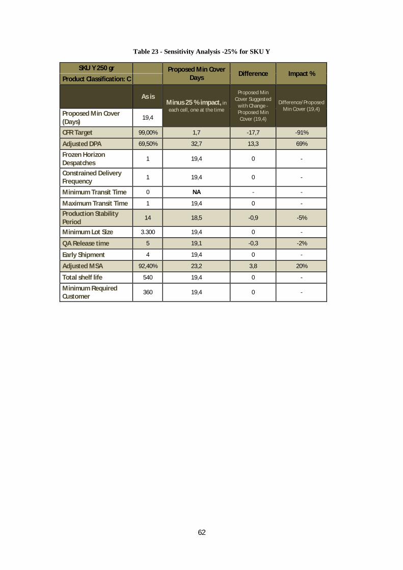
62

Table 23 - Sensitivity Analysis -25% for SKU Y

SKU Y 250 gr Proposed Min Cover Days Difference Impact %

Product Classification: C

As is Minus 25 % impact, in

each cell, one at the time

Proposed Min Cover Suggested

with Change - Proposed Min Cover (19,4)

Difference/Proposed Min Cover (19,4)

Proposed Min Cover (Days)

19,4

CFR Target 99,00% 1,7 -17,7 -91%

Adjusted DPA 69,50% 32,7 13,3 69%

Frozen Horizon Despatches

1 19,4 0 -

Constrained Delivery Frequency 1 19,4 0 -

Minimum Transit Time 0 NA - -

Maximum Transit Time 1 19,4 0 -

Production Stability Period

14 18,5 -0,9 -5%

Minimum Lot Size 3.300 19,4 0 -

QA Release time 5 19,1 -0,3 -2%

Early Shipment 4 19,4 0 -

Adjusted MSA 92,40% 23,2 3,8 20%

Total shelf life 540 19,4 0 -

Minimum Required Customer

360 19,4 0 -

63

Table 24 - Sensitivity Analysis -25% for SKU Z

SKU Z 300 gr Proposed Min Cover Days Difference Impact %

Product Classification: A

As is Minus 25 % impact, in each cell, one at the time

Proposed Min Cover Suggested

with Change - Proposed Min Cover (13,4)

Difference/Proposed Min Cover (13,4)

Proposed Min Cover (Days)

13,4

CFR Target 99,00% 2 -11,4 -85%

Adjusted DPA 77,70% 27,3 13,4 100%

Frozen Horizon Despatches

7 13,4 0

Constrained Delivery Frequency 1 13,4 0 -

Minimum Transit Time 1 NA - -

Maximum Transit Time 3 13,4 0 -

Production Stability Period

14 12,7 -0,7 -5%

Minimum Lot Size 2.000 13,4 0 -

QA Release time 6 13,1 -0,3 -2%

Early Shipment 0 NA - -

Adjusted MSA 85,30% 16,1 2,7 20%

Total shelf life 540 13,4 0 -

Minimum Required Customer 360 13,4 0 -

64

Appendix II

Figure 14 – SKU W Calculation

SKU

Mad

Bul

l3

0 -1

Mon

th3

Mor

e th

an 1

000

PUM

's3

Less

than

87

%3

A 3

High

ly P

rom

oted

3M

arke

t's B

et3

Less

or e

qual

to 5

% o

f PU

M's

of it

s cat

egor

y3

Hors

e2

2 M

onth

250

0 to

100

0 PU

M's

287

% -

92 %

2B

2Av

erag

e Pr

omot

ed2

Good

Beh

avio

ur2

5 to

10%

of P

UM's

of

its ca

tego

ry2

Jack

Rab

it1

3 M

onth

110

0 to

500

PUM

's1

Mor

e th

an 9

2 %

1C

1Lo

w P

rom

oted

1Ba

d Be

havi

our

110

to 1

5% o

f PUM

's of

its

cate

gory

1

Mul

e0

Mor

e th

an 3

mth

.0

0 to

100

PUM

's0

00

00

Mor

e th

an 1

5% o

f PU

M's

of it

s cat

egor

y0

Wei

ght

Tota

l

SKU

Pont

uati

on

SKU

Perc

enta

ge

ABC

Prom

oted

SKU

SKU

Bet

Clas

sific

atio

nAn

imal

Far

mPo

sitiv

e Bi

asO

OS

MSA

0,30

0,

30

20,0

%10

,0%

20,0

%10

,0%

10,0

%

0,60

-

-

0,

20

0,30

Max

imum

Pos

sibl

e Po

ntua

tion

of a

SKU

from

this

Cat

egor

y

(S

um o

f all

max

imum

pon

tuat

ion

from

diff

SKU

's)

W

13,9

10,6

Curr

ent M

inim

umM

inim

um S

ugge

sted

by

Opt

imiz

er T

ool

Min

imum

Adj

uste

d by

the

Clas

sific

atio

n

Pare

to A

naly

sis b

ased

on

PU

M's

10,0

%

0,20

2,50

0

8 Da

ys

1,90

76,0

%

10,0

%10

,0%

65

Figure 15 – SKU X Calculation

SKU

Mad

Bul

l3

0 -1

Mon

th3

Mor

e th

an 1

000

PUM

's3

Less

than

87

%3

A 3

High

ly P

rom

oted

3M

arke

t's B

et3

Less

or e

qual

to 5

% o

f PU

M's

of it

s cat

egor

y3

Hors

e2

2 M

onth

250

0 to

100

0 PU

M's

287

% -

92 %

2B

2Av

erag

e Pr

omot

ed2

Good

Beh

avio

ur2

5 to

10%

of P

UM's

of

its ca

tego

ry2

Jack

Rab

it1

3 M

onth

110

0 to

500

PUM

's1

Mor

e th

an 9

2 %

1C

1Lo

w P

rom

oted

1Ba

d Be

havi

our

110

to 1

5% o

f PUM

's of

its

cate

gory

1

Mul

e0

Mor

e th

an 3

mth

.0

0 to

100

PUM

's0

00

00

Mor

e th

an 1

5% o

f PU

M's

of it

s cat

egor

y0

Wei

ght

Tota

l

SKU

Pont

uatio

n SK

U Pe

rcen

tage

X

Clas

sific

atio

nAn

imal

Far

mPo

sitiv

e Bi

asO

OS

MSA

AB

CPr

omot

ed S

KUSK

U B

etPa

reto

Ana

lysi

s bas

ed

on P

UM

's

10,0

%10

,0%

0,40

-

0,20

0,

10

0,20

0,20

0,

20

0,20

20,0

%10

,0%

20,0

%10

,0%

10,0

%10

,0%

Min

imum

Sug

gest

ed b

y O

ptim

izer

Too

l15

,7

Min

imum

Adj

uste

d by

the

Clas

sific

atio

n9,

4

1,50

Max

imum

Pos

sibl

e Po

ntua

tion

of a

SKU

from

this

Cat

egor

y

(S

um o

f all

max

imum

pon

tuat

ion

from

diff

SKU

's)

2,50

0

60,0

%

Curr

ent M

inim

um10

Day

s

66

Figure 16 – SKU Y Calculation

SKU

Mad

Bul

l3

0 -1

Mon

th3

Mor

e th

an 1

000

PUM

's3

Less

than

87

%3

A 3

High

ly P

rom

oted

3M

arke

t's B

et3

Less

or e

qual

to 5

% o

f PU

M's

of it

s cat

egor

y3

Hors

e2

2 M

onth

250

0 to

100

0 PU

M's

287

% -

92 %

2B

2Av

erag

e Pr

omot

ed2

Good

Beh

avio

ur2

5 to

10%

of P

UM's

of

its ca

tego

ry2

Jack

Rab

it1

3 M

onth

110

0 to

500

PUM

's1

Mor

e th

an 9

2 %

1C

1Lo

w P

rom

oted

1Ba

d Be

havi

our

110

to 1

5% o

f PUM

's of

its

cate

gory

1

Mul

e0

Mor

e th

an 3

mth

.0

0 to

100

PUM

's0

00

00

Mor

e th

an 1

5% o

f PU

M's

of it

s cat

egor

y0

Wei

ght

Tota

l

SKU

Pont

uatio

n SK

U Pe

rcen

tage

Y

Clas

sific

atio

nAn

imal

Far

mPo

sitiv

e Bi

asO

OS

MSA

AB

CPr

omot

ed S

KUSK

U B

etPa

reto

Ana

lysi

s bas

ed

on P

UM

's

10,0

%10

,0%

0,20

-

-

0,

10

0,10

0,20

0,

30

0,20

20,0

%10

,0%

20,0

%10

,0%

10,0

%10

,0%

Min

imum

Sug

gest

ed b

y O

ptim

izer

Too

l15

,4

Min

imum

Adj

uste

d by

the

Clas

sific

atio

n6,

8

1,10

Max

imum

Pos

sibl

e Po

ntua

tion

of a

SKU

from

this

Cat

egor

y

(S

um o

f all

max

imum

pon

tuat

ion

from

diff

SKU

's)

2,50

0

44,0

%

Curr

ent M

inim

um11

Day

s

67

Figure 17 – SKU Z Calculation

SKU

Mad

Bul

l3

0 -1

Mon

th3

Mor

e th

an 1

000

PUM

's3

Less

than

87

%3

A 3

High

ly P

rom

oted

3M

arke

t's B

et3

Less

or e

qual

to 5

% o

f PU

M's

of it

s cat

egor

y3

Hors

e2

2 M

onth

250

0 to

100

0 PU

M's

287

% -

92 %

2B

2Av

erag

e Pr

omot

ed2

Good

Beh

avio

ur2

5 to

10%

of P

UM's

of

its ca

tego

ry2

Jack

Rab

it1

3 M

onth

110

0 to

500

PUM

's1

Mor

e th

an 9

2 %

1C

1Lo

w P

rom

oted

1Ba

d Be

havi

our

110

to 1

5% o

f PUM

's of

its

cate

gory

1

Mul

e0

Mor

e th

an 3

mth

.0

0 to

100

PUM

's0

00

00

Mor

e th

an 1

5% o

f PU

M's

of it

s cat

egor

y0

Wei

ght

Tota

l

SKU

Pon

tuat

ion

SKU

Per

cent

age

Z

Clas

sific

atio

nAn

imal

Far

mPo

sitiv

e Bi

asO

OS

MSA

AB

CPr

omot

ed S

KUSK

U B

etPa

reto

Ana

lysi

s bas

ed

on P

UM

's

10,0

%10

,0%

0,40

0,20

-

0,

30

0,20

0,10

0,

20

0,30

20,0

%10

,0%

20,0

%10

,0%

10,0

%10

,0%

Min

imum

Sug

gest

ed b

y O

ptim

izer

Too

l15

,3

Min

imum

Adj

uste

d by

the

Clas

sific

atio

n10

,4

1,70

Max

imum

Pos

sibl

e Po

ntua

tion

of a

SKU

from

this

Cat

egor

y

(S

um o

f all

max

imum

pon

tuat

ion

from

diff

SKU

's)

2,50

0

68,0

%

Curr

ent M

inim

um12

Day

s