Reducing Hospital Readmissions by Integrating Empirical …helmjweb/publications/A5 (POM) Re… ·...

Reducing Hospital Readmissions by IntegratingEmpirical Prediction with Resource Optimization

Jonathan E. HelmOperations and Decision Technologies, Kelley School of Business, Indiana University, 1309 E. Tenth Street, Bloomington, Indiana 47405,

USA, [email protected]

Adel AlaeddiniDepartment of Mechanical Engineering, University of Texas, San Antonio One UTSA Circle, San Antonio, Texas 78249, USA

[email protected]

Jon M. Stauffer, Kurt M. BretthauerOperations and Decision Technologies, Kelley School of Business, Indiana University, 1309 E. Tenth Street, Bloomington, Indiana 47405,

USA, [email protected], [email protected]

Ted A. SkolarusDepartment of Urology, University of Michigan, VA, Health Services Research & Development (HSR&D) Center for Clinical ManagementResearch, VA, Ann Arbor Healthcare System, 3875 Taubman Center, 1500 East Medical Center Drive, Ann Arbor, Michigan 48109, USA

[email protected]

H ospital readmissions present an increasingly important challenge for health-care organizations. Readmissions areexpensive and often unnecessary, putting patients at risk and costing $15 billion annually in the United States

alone. Currently, 17% of Medicare patients are readmitted to a hospital within 30 days of initial discharge with readmis-sions typically being more expensive than the original visit to the hospital. Recent legislation penalizes organizations witha high readmission rate. The medical literature conjectures that many readmissions can be avoided or mitigated by post-discharge monitoring. To develop a good monitoring plan it is critical to anticipate the timing of a potential readmissionand to effectively monitor the patient for readmission causing conditions based on that knowledge. This research developsnew methods to empirically generate an individualized estimate of the time to readmission density function and then usesthis density to optimize a post-discharge monitoring schedule and staffing plan to support monitoring needs. Ourapproach integrates classical prediction models with machine learning and transfer learning to develop an empirical den-sity that is personalized to each patient. We then transform an intractable monitoring plan optimization with stochasticdischarges and health state evolution based on delay-time models into a weakly coupled network flow model with tracta-ble subproblems after applying a new pruning method that leverages the problem structure. Using this multi-methodolog-ic approach on two large inpatient datasets, we show that optimal readmission prediction and monitoring plans canidentify and mitigate 40–70% of readmissions before they generate an emergency readmission.

Key words: hospital readmissions; post-discharge patient monitoring; readmission risk profiling; Bayesian survival analy-sis; delay-time models of readmissionsHistory: Received: December 2013; Accepted: December 2014 by Tsan-Ming Choi, after 1 revision.

1. Introduction

Hospital and medical center readmissions is a serioushealth-care issue demanding increased attention ascosts continue to rise and patient care suffers. Basedon a report to Congress in 2008, over 17% of Medicarepatients were readmitted in the first 30 days after dis-charge, accounting for more than $15 billion dollarsper year (Foster and Harkness 2010). Not only arereadmissions expensive, recent studies have alsolinked the rate of readmission to quality of care inmedical centers (e.g., Halfon et al. 2006). Surprisingly,

Foster and Harkness (2010) found that a significantpercent of readmissions are avoidable through betterpost-discharge management; of the $15 billion spent,$12 billion was associated with potentially preventablereadmissions. Current strategies to reduce readmis-sions focus on (i) identifying high-risk patients (e.g.,Kansagara et al. 2011, Rosenberg et al. 2007, Wall-mann et al. 2013), or (ii) developing an effective planfor post-discharge care (e.g., Jack et al. 2009). Whilethese heuristic clinical approaches have proven effec-tive in avoiding readmissions, there remains signifi-cant opportunity for an approach that combines

233

Vol. 25, No. 2, February 2016, pp. 233–257 DOI 10.1111/poms.12377ISSN 1059-1478|EISSN 1937-5956|16|2502|0233 © 2015 Production and Operations Management Society

rigorous empirical modeling to predict time to read-mission with optimization to design schedules andallocate staff for post-discharge monitoring. To havethe largest possible impact on readmissions, it is nec-essary to know both when a patient is likely to be re-admitted (empirical prediction model) and when tomonitor that patient to identify the condition before ittriggers a readmission (optimization model). Thisstudy represents a multi-methodology effort aimed atintegrating clinical, statistical, and operations man-agement techniques to (i) quantify post-discharge riskof readmission for each patient over time, (ii) todesign optimal post-discharge treatment plans forearly detection and avoidance of potential readmis-sions, and (iii) to allocate sufficient system capacity tobe able to administer the optimal treatment plans fora cohort of patients.Numerous efforts have focused on capturing the

key dynamics of the readmission system (Desai et al.2009, Kansagara et al. 2011). The study of readmissionrisk factors typically falls into three major categories:(i) patient attributes such as history of readmission,severity of illness, comorbidity, age, gender, life satis-faction, change in clinical variables, source of pay-ment, etc. (e.g., Dunlay et al. 2009, Wallmann et al.2013, Watson et al. 2011); (ii) factors targeting the pre-discharge process including length of stay, adequacyof discharge plan, nursing environment of the hospi-tal, characteristics of the physician, etc., (e.g., McHughand Ma 2013, Rosen et al. 2013); and finally (iii) fac-tors targeting the post-discharge process includinginadequacy of post-discharge planning and followup, non-compliance with medication and diet, failedsocial support, impairment of self-care, etc. (e.g., Her-nandez et al. 2010, Wallmann et al. 2013, Watsonet al. 2011). Using the above risk factors a number ofhealth-care systems have started implementing onlinereadmission risk calculators. Some of these calculatorsmay be found at http://riskcalc.sts.org/STSWebRisk-Calc273/, by the Society of Thoracic Surgeons whichpredicts the risk of operative mortality and morbidityafter adult cardiac surgery, and at http://www.read-missionscore.org, by the Center for OutcomesResearch and Evaluation (CORE), which helps predicta patient’s likelihood of readmission for heart failurewithin 30 days of discharge. Despite their benefits,these calculators have serious limitations. They (i)assume homogeneity of the population and hospital’sperformance; (ii) provide no estimate on time to read-mission; and (iii) provide no guidance on how to usethe estimates to make better care decisions. Our meth-ods will address these deficiencies.Recently, researchers have begun to investigate the

impact of targeted discharge planning and post-discharge management on reducing readmissions,focusing on financial incentives/cost-effectiveness,

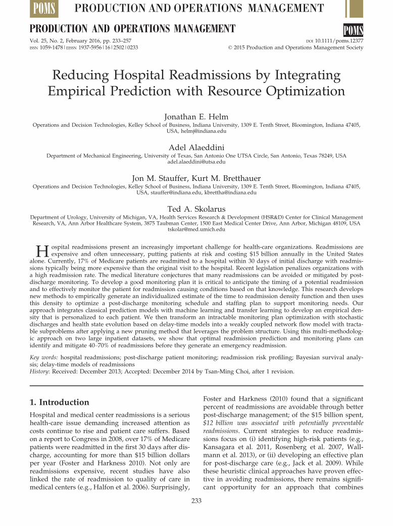
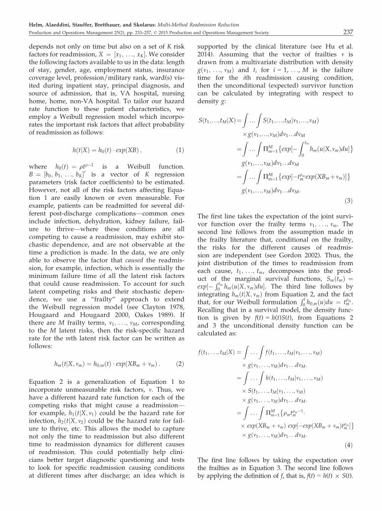
pre-discharge patient education, and improved post-discharge management. In particular, several studiesclaim that post-discharge management can reducereadmissions by 12% to 30% (see Gonseth et al. 2004)and as high as 85% (see Fonarow et al. 1997) by target-ing high-risk populations (see Minott 2008, Wolinskyet al. 2009), telemonitoring (see Graham et al. 2012),and other monitoring strategies. By integratingpatient risk calculations and empirical predictions oftime to readmission with optimization methods todesign monitoring plans, we capture both of thehigh-impact approaches (risk profiling and plannedmonitoring) from the medical literature in a quantitativeframework for optimally designing these post-dischargemonitoring plans that are currently designed usingexpert judgment or ad hoc approaches.Figure 1 provides a high-level overview of our

multi-methodology approach which uses both read-mission prediction and follow-up schedule optimi-zation to reduce readmissions. First the EmpiricalPrediction Model utilizes individual patient data todetermine a probability of readmission andexpected time to readmission for each patient. Thesepatient and procedure specific readmission curvesare then aggregated with K-mean clustering (orother methods) into several different risk profiles.The aggregated readmission curves for each riskprofile, organization-specific resource capacity and

Individual Patient Data:• Demographic Data• Health History

• Hospital Stay Data

Individual Patient Estimates:• Probability of Readmission• Time to Readmission

Patient ReadmissionCosts and Savings

Patient Follow-up ScheduleRequired Hospital Resources

Empirical Prediction Model

Aggregation into Risk Profiles

Optimization Model

Hospital Follow-upCapacity and Costs

Figure 1 Multi-Methodology Model Overview

Helm, Alaeddini, Stauffer, Bretthauer, and Skolarus: Multi-Method Readmission Reduction234 Production and Operations Management 25(2), pp. 233–257, © 2015 Production and Operations Management Society

http://riskcalc.sts.org/STSWebRiskCalc273/

http://riskcalc.sts.org/STSWebRiskCalc273/

http://www.readmissionscore.org

http://www.readmissionscore.org

cost information, and medical procedure-specific re-admission cost and savings information are all usedas inputs into the Optimization Model. The Optimi-zation Model uses these inputs to determine anoptimal follow-up schedule for each patient riskprofile and determine the number of resources thehospital or health system will need to execute allexpected follow-up schedules.While previous literature relies on a siloed

approach, focusing either on predicting readmissionsor on strategies to reduce readmissions, this researchintegrates the two using advanced mathematical, sta-tistical, and operations management techniques com-bined with clinical expertise. We not only develop anintegrative framework for investigating both aspectsof readmission modeling simultaneously, we alsocontribute new methods to each of the areas. To thebest of our knowledge, existing studies have noteffectively considered heterogeneity among patientpopulations, and are not able to adapt population-based readmission estimates to individual patients.Further, previous readmission prediction modelshave only focused on small groups of patients with asingle readmission triggering condition (e.g., elderlycardiovascular patients), and the results are often notgeneralizable to other cases (see Feudtner et al. 2009,Gonseth et al. 2004). In addition, most of the availablestudies have not effectively used the array of avail-able machine-learning techniques to improve theirresults. This study addresses these deficiencies byenabling individualized readmission probability esti-mates and a generalizable method that can encom-pass diverse patient populations and multiplereadmission causing conditions over an arbitrary timeperiod. Further, existing models have been lackingcomprehensive optimization approaches to designtailored post-discharge management plans. No litera-ture to our knowledge captures, as we intend to do,the health-care organization’s ability to support alarge-scale implementation of a post-dischargemanagement scheme that simultaneously solves forpost-discharge monitoring timing and the organiza-tional resource capacity needed to implement suchschedules.Finally, we demonstrate how this multi-methodol-

ogy approach can be applied via an extensive casestudy and numerical analysis using two differentdatasets from (i) a partner hospital in Michiganincluding 2449 patients with 17 diagnoses, 3108 read-missions, and 15 demographic, socioeconomic, andclinical factors, etc. (ii) the State Inpatient Databases(SID) for 5000 patients diagnosed with bladder, kid-ney, and prostate cancer in 2009 along with other can-cers (see http://www.hcup-us.ahrq.gov/db/state/siddist/SID_Introduction.jsp). The results for the twodatasets were structurally similar, so for the purposes

of cohesive exposition we focus on the results fromthe partner hospital in Michigan for this study.Section 2 develops the empirical model to predict

readmission occurrence and timing. Section 3 uses thepredicted empirical readmission density from section2 to develop a follow-up schedule for patients andstaffing plan for a follow-up organization. Section 4brings both components together, empirical predic-tion and resource optimization, in a case study usinghistorical inpatient readmission data to design a prac-tical post-discharge monitoring schedule and gener-ate insights into tactical and operational managementof post-discharge care. These results confirm the con-jecture in the medical literature that between 12% and85% of readmissions can be avoided or identifiedearly through better post-discharge plans and showhow to effectively design such plans. Section 5 con-cludes the study.

2. Stage 1: Empirical Modeling toPredict Time to Readmission

While a number of studies have focused on predictingwhether or not a patient will be readmitted within30 days (see van Walraven et al. 2010), there is onlyone article to our knowledge that focuses on predict-ing the time to readmission (see Yu et al. 2013). WhileYu et al. (2013) shares similarities with our work,there are important differences in the two approaches.From a methodological perspective Yu et al. (2013),among other studies, does not consider which condi-tion has caused the readmission, for example, infec-tion, dehydration, kidney failure etc. We are able tocapture this feature using a frailty approach to modelthese conditions as latent competing risks with sto-chastic dependence. In addition, Yu et al. (2013),among others, use a population-based approachbased on equally weighted readmission records froma specific hospital to calculate the risk of readmissionfor that hospital’s patients. However, we employtransfer learning to weight the readmission records inthe dataset based on their similarity to the readmis-sion record(s) for the patient of interest to: (i) furtherpersonalize the estimate and (ii) alleviate the problemof data scarcity. Finally, Yu et al. (2013), along withother readmission prediction models, gives the sameimportance to all readmission records regardless ofhow recently the readmission occurred. Our methodassigns importance (weight) to the admission/read-mission records based on record recency (more recentrecords get more weight) using an optimizationprocess to choose the appropriate weights. Thisaccounts for the phenomenon that each patient’shealth status and/or behaviors can change over time.From the specific modeling perspective, we use aBayesian approach while Yu et al. (2013) uses a

Helm, Alaeddini, Stauffer, Bretthauer, and Skolarus: Multi-Method Readmission Reduction

Production and Operations Management 25(2), pp. 233–257, © 2015 Production and Operations Management Society 235

http://www.hcup-us.ahrq.gov/db/state/siddist/SID_Introduction.jsp

http://www.hcup-us.ahrq.gov/db/state/siddist/SID_Introduction.jsp

classical approach. Further, we employ a parsimoni-ous prior while Yu et al. (2013) employs a forwardselection procedure for identifying the most importantvariables.Understanding the time to readmission is critical to

making clinically effective decisions to mitigatepotential readmissions, such as when to follow upwith a patient who has been discharged from the hos-pital. In this section, we develop empirical predictionmodels to accurately capture the probability distribu-tion on time to readmission based on two differentdatasets (the State Inpatient Database (SID) as well asa dataset from a partner hospital in Michigan) toshow that our methods can be used broadly (e.g., onSID) or tailored to a specific hospital.Beyond exploring the new area of predicting time

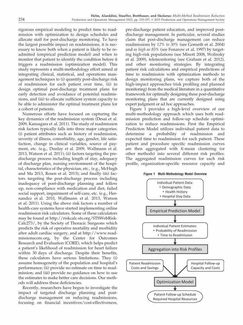
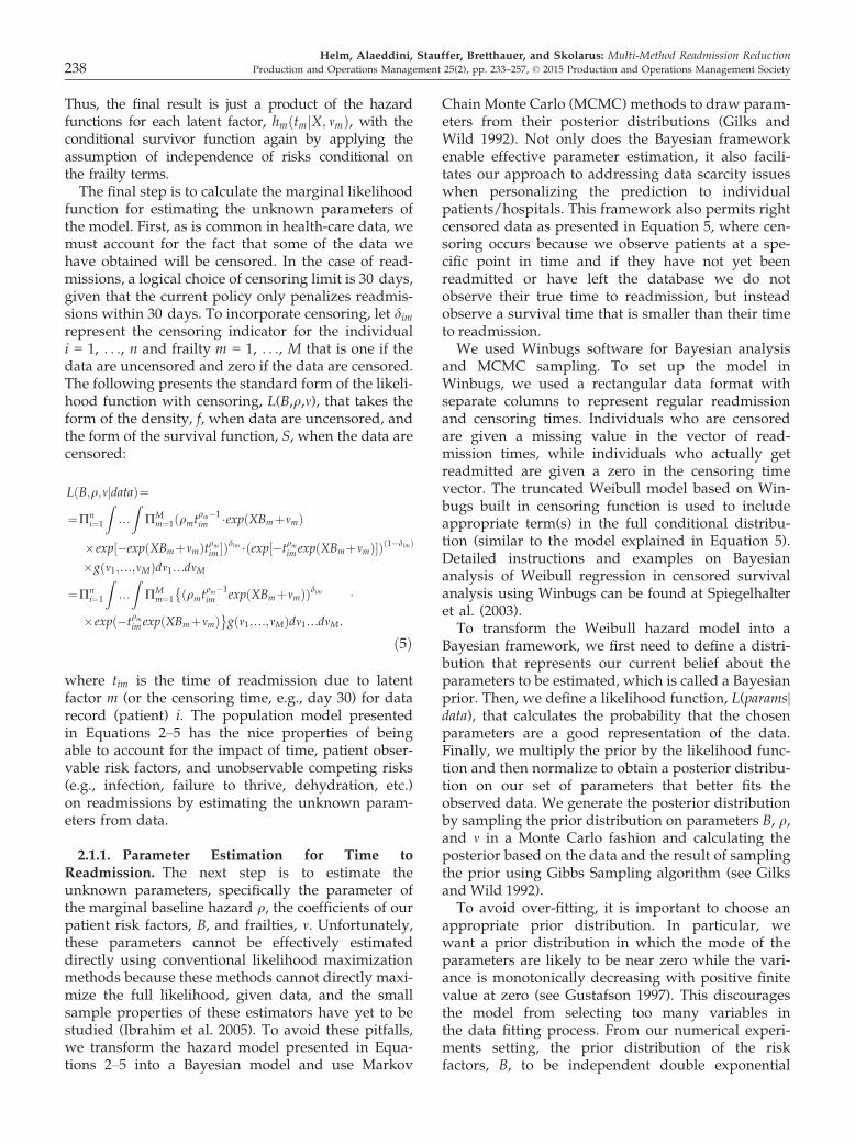
to readmission, we also address two other featuresthat are prevalent in health care: (i) the need to per-sonalize the prediction method to each individualpatient, and (ii) scarcity of relevant data. The result ofthe empirical modeling in this section is a set of tai-lored probability distributions (one for each individ-ual patient) that is personalized for each patient inour datasets. Our approach builds up the predictionmodel through three steps as shown in Figure 2. Step1 (section 2.1) develops a general population estimatefor time to readmission, which accounts for demo-graphic, socioeconomic, health history, co-morbidity,the hospital the patient was treated at, and other rele-vant patient and system characteristics. In section 2.1,we also discuss how we are able to incorporate thecause of readmission into our prediction model. Wedo so by developing a Weibull regression model thatincorporates observable and unobservable risk factors.The model from Step 1 is then personalized in Step

2 (section 2.2) by parameterizing the Weibull modelusing each patient’s personal history of hospitaladmissions and readmissions to date. Step 3 (also sec-tion 2.2) addresses the problem of data scarcity, whichoccurs when an individual has too few prior recordsto adequately parameterize the model with their indi-vidual data alone (Step 2) and when applying themethod to a new hospital or group that has little rele-vant data. For example, when personalizing the read-mission estimate, we are able to use data from allpatients in our dataset (not just from the patientwhose time to readmission curve is currently being

estimated), by adding weights to the data records.Higher weights indicate a higher level of statisticalsimilarity of any given patient in the dataset with thetarget patient. This approach, called transfer learning,and the specifics of calculating and incorporatingweights are discussed in section 2.2.In section 2.3 we discuss the methods and algo-

rithms used to apply the approaches in sections 2.1and 2.2 to our real-world datasets. While the dataabout a particular individual or specific hospital maybe small, the overall dataset we intend the model towork with will be large. With large datasets, the com-mon methods for prediction have significant draw-backs. For example, machine learning often suffersfrom results being difficult to interpret and sometimesyields patterns that are a product of random fluctua-tions, while more classical prediction models employoversimplifying assumptions that lead to incorrectconclusions. To overcome these limitations, wedevelop an empirical prediction model that integratesboth classical prediction methods with machine learn-ing using a Bayesian framework. We conclude thesection by comparing the accuracy of our predictionmodel against other commonly used prediction mod-els in the literature.

2.1. Population-Based Model of Time toReadmissionWe begin by building a population-based estimate oftime to readmission in which we consider the impactof (i) time after initial discharge from the hospital, (ii)patient-specific risk factors impacting likelihood of re-admission, and (iii) unobservable or random effectsthat capture patient heterogeneity. We capture time toreadmission using a Weibull regression model. Webegin with a hazard rate function, h(t). In our optimi-zation model presented in section 3, this hazard ratecan be used to model the deterministic arrival ratefunction of a non-homogeneous Poisson process(NHPP) capturing the arrival of readmission-causingfailures (as is common in delay-time analysis), how-ever, the NHPP assumption is not necessary for esti-mation of the survival model. The probability that apatient has not yet been readmitted by time t is there-

fore given by SðtÞ ¼ exp �R t0 hðuÞdu

� �, which we call

the survival function. The hazard function, however,

Data Source

All Patients: Demographic, Socio-Economic, Health History, Comorbidity, etc. Individual patient’s re/admission records

Purpose

Generalized correlated frailty model

Population Estimate of Readmissions Personalized Prediction for each

Individual Patient Increasing Prediction Accuracy by

Including Data from Similar Patients

Similarity among patients’ readmission records

Bayesian Inference, Markov Chain Monte Carlo Methods

Local regression & similarity index, Bayesian weighting, titled time framing

Step 1 Step 3 Step 2

Methods

Figure 2 Framework for Predicting Patient Readmissions


depends not only on time but also on a set of K riskfactors for readmission, X ¼ ½x1; . . .; xK�. We considerthe following factors available to us in the data: lengthof stay, gender, age, employment status, insurancecoverage level, profession/military rank, ward(s) vis-ited during inpatient stay, principal diagnosis, andsource of admission, that is, VA hospital, nursinghome, home, non-VA hospital. To tailor our hazardrate function to these patient characteristics, weemploy a Weibull regression model which incorpo-rates the important risk factors that affect probabilityof readmission as follows:

hðtjXÞ ¼ h0ðtÞ � expðXBÞ ; ð1Þ

where h0ðtÞ ¼ qtq�1 is a Weibull function.B ¼ ½b0; b1; . . .; bK�0 is a vector of K regressionparameters (risk factor coefficients) to be estimated.However, not all of the risk factors affecting Equa-tion 1 are easily known or even measurable. Forexample, patients can be readmitted for several dif-ferent post-discharge complications—common onesinclude infection, dehydration, kidney failure, fail-ure to thrive—where these conditions are allcompeting to cause a readmission, may exhibit sto-chastic dependence, and are not observable at thetime a prediction is made. In the data, we are onlyable to observe the factor that caused the readmis-sion, for example, infection, which is essentially theminimum failure time of all the latent risk factorsthat could cause readmission. To account for suchlatent competing risks and their stochastic depen-dence, we use a “frailty” approach to extendthe Weibull regression model (see Clayton 1978,Hougaard and Hougaard 2000, Oakes 1989). Ifthere are M frailty terms, m1; . . .; mM, correspondingto the M latent risks, then the risk-specific hazardrate for the mth latent risk factor can be written asfollows:

hmðtjX; mmÞ ¼ h0;mðtÞ � expðXBm þ mmÞ : ð2Þ

Equation 2 is a generalization of Equation 1 toincorporate unmeasurable risk factors, m. Thus, wehave a different hazard rate function for each of thecompeting risks that might cause a readmission—for example, h1ðtjX; m1Þ could be the hazard rate forinfection, h2ðtjX; m2Þ could be the hazard rate for fail-ure to thrive, etc. This allows the model to capturenot only the time to readmission but also differenttime to readmission dynamics for different causesof readmission. This could potentially help clini-cians better target diagnostic questioning and teststo look for specific readmission causing conditionsat different times after discharge; an idea which is

supported by the clinical literature (see Hu et al.2014). Assuming that the vector of frailties m isdrawn from a multivariate distribution with densitygðm1; . . .; mMÞ and ti for i = 1, . . ., M is the failuretime for the ith readmission causing condition,then the unconditional (expected) survivor functioncan be calculated by integrating with respect todensity g:

Sðt1;...;tMjXÞ¼Z

...

ZSðt1;...;tMjm1;...;mMÞ

�gðm1;...;mMÞdm1...dmM

¼Z

...

ZPM

m¼1

�exp½�

Z tm

0

hmðujX;mmÞdu��

gðm1;...;mMÞdm1...dmM

¼Z

...

ZPM

m¼1

�exp½�tqmm expðXBmþmmÞ�

�gðm1;...;mMÞdm1...dmM:

ð3Þ

The first line takes the expectation of the joint survi-vor function over the frailty terms m1; . . .; mm. Thesecond line follows from the assumption made inthe frailty literature that, conditional on the frailty,the risks for the different causes of readmis-sion are independent (see Gordon 2002). Thus, thejoint distribution of the times to readmission fromeach cause, t1; . . .; tm, decomposes into the prod-uct of the marginal survival functions, SmðtmÞ ¼exp½�

R tm0 hmðujX; mmÞdu�. The third line follows by

integrating hmðtjX; mmÞ from Equation 2, and the factthat, for our Weibull formulation

R t0 h0;mðuÞdu ¼ tqmm .

Recalling that in a survival model, the density func-tion is given by f(t) = h(t)S(t), from Equations 2and 3 the unconditional density function can becalculated as:

fðt1; . . .; tMjXÞ ¼Z

. . .

Zfðt1; . . .; tMjm1; . . .; mMÞ

� gðm1; . . .; mMÞdm1. . .dmM:

¼Z

. . .

Zhðt1; . . .; tMjm1; . . .; mMÞ

� Sðt1; . . .; tMjm1; . . .; mMÞ� gðm1; . . .; mMÞdm1. . .dmM:

¼Z

. . .

ZPM

m¼1

�qmt

qm�1m �

� expðXBm þ mmÞ exp½�expðXBm þ mmÞtqmm ��

� gðm1; . . .; mMÞdm1. . .dmM:

ð4Þ

The first line follows by taking the expectation overthe frailties as in Equation 3. The second line followsby applying the definition of f, that is, f(t) = h(t) 9 S(t).



Thus, the final result is just a product of the hazardfunctions for each latent factor, hmðtmjX; mmÞ, with theconditional survivor function again by applying theassumption of independence of risks conditional onthe frailty terms.The final step is to calculate the marginal likelihood

function for estimating the unknown parameters ofthe model. First, as is common in health-care data, wemust account for the fact that some of the data wehave obtained will be censored. In the case of read-missions, a logical choice of censoring limit is 30 days,given that the current policy only penalizes readmis-sions within 30 days. To incorporate censoring, let dimrepresent the censoring indicator for the individuali = 1, . . ., n and frailty m = 1, . . ., M that is one if thedata are uncensored and zero if the data are censored.The following presents the standard form of the likeli-hood function with censoring, L(B,q,m), that takes theform of the density, f, when data are uncensored, andthe form of the survival function, S, when the data arecensored:

LðB;q;mjdataÞ¼

¼Pni¼1

Z...

ZPM

m¼1ðqmtqm�1im �expðXBmþmmÞ

�exp½�expðXBmþmmÞtqmim �Þdim �ðexp½�tqmim expðXBmþmmÞ�Þð1�dimÞ

�gðm1;...;mMÞdm1...dmM

¼Pni¼1

Z...

ZPM

m¼1

�ðqmt

qm�1im expðXBmþmmÞÞdim �

�expð�tqmim expðXBmþmmÞ�gðm1;...;mMÞdm1...dmM:

ð5Þ

where tim is the time of readmission due to latentfactor m (or the censoring time, e.g., day 30) for datarecord (patient) i. The population model presentedin Equations 2–5 has the nice properties of beingable to account for the impact of time, patient obser-vable risk factors, and unobservable competing risks(e.g., infection, failure to thrive, dehydration, etc.)on readmissions by estimating the unknown param-eters from data.

2.1.1. Parameter Estimation for Time toReadmission. The next step is to estimate theunknown parameters, specifically the parameter ofthe marginal baseline hazard q, the coefficients of ourpatient risk factors, B, and frailties, m. Unfortunately,these parameters cannot be effectively estimateddirectly using conventional likelihood maximizationmethods because these methods cannot directly maxi-mize the full likelihood, given data, and the smallsample properties of these estimators have yet to bestudied (Ibrahim et al. 2005). To avoid these pitfalls,we transform the hazard model presented in Equa-tions 2–5 into a Bayesian model and use Markov

Chain Monte Carlo (MCMC) methods to draw param-eters from their posterior distributions (Gilks andWild 1992). Not only does the Bayesian frameworkenable effective parameter estimation, it also facili-tates our approach to addressing data scarcity issueswhen personalizing the prediction to individualpatients/hospitals. This framework also permits rightcensored data as presented in Equation 5, where cen-soring occurs because we observe patients at a spe-cific point in time and if they have not yet beenreadmitted or have left the database we do notobserve their true time to readmission, but insteadobserve a survival time that is smaller than their timeto readmission.We used Winbugs software for Bayesian analysis

and MCMC sampling. To set up the model inWinbugs, we used a rectangular data format withseparate columns to represent regular readmissionand censoring times. Individuals who are censoredare given a missing value in the vector of read-mission times, while individuals who actually getreadmitted are given a zero in the censoring timevector. The truncated Weibull model based on Win-bugs built in censoring function is used to includeappropriate term(s) in the full conditional distribu-tion (similar to the model explained in Equation 5).Detailed instructions and examples on Bayesiananalysis of Weibull regression in censored survivalanalysis using Winbugs can be found at Spiegelhalteret al. (2003).To transform the Weibull hazard model into a

Bayesian framework, we first need to define a distri-bution that represents our current belief about theparameters to be estimated, which is called a Bayesianprior. Then, we define a likelihood function, L(params|data), that calculates the probability that the chosenparameters are a good representation of the data.Finally, we multiply the prior by the likelihood func-tion and then normalize to obtain a posterior distribu-tion on our set of parameters that better fits theobserved data. We generate the posterior distributionby sampling the prior distribution on parameters B, q,and m in a Monte Carlo fashion and calculating theposterior based on the data and the result of samplingthe prior using Gibbs Sampling algorithm (see Gilksand Wild 1992).To avoid over-fitting, it is important to choose an

appropriate prior distribution. In particular, wewant a prior distribution in which the mode of theparameters are likely to be near zero while the vari-ance is monotonically decreasing with positive finitevalue at zero (see Gustafson 1997). This discouragesthe model from selecting too many variables inthe data fitting process. From our numerical experi-ments setting, the prior distribution of the riskfactors, B, to be independent double exponential


random variables, using multivariate normal distri-bution to represent the joint distribution of the frail-ties, mm, and choosing a gamma distribution for theparameter of the marginal baseline hazard, qm, per-formed well for our data. In the next section, weshow how we can employ transfer learning toparameterize our Weibull regression modeldescribed in this section with enough data and yetstill personalize the readmission prediction.

2.2. Personalizing Readmission Predictions andData ScarcityA key feature of health-care modeling is the need topersonalize prediction and forecasting models toaccount for individual patient characteristics becauseaggregate population-based models do not often per-form well on a patient-by-patient basis. Personalizingtime to readmission predictions also enables us todevelop risk profiles that allow us to tailor our moni-toring decision framework in section 3 and signifi-cantly outperform a population-based monitoringplan. To obtain a population-based estimate, we sim-ply use all the data available in our datasets in thelikelihood function, L (Equation 5), when estimatingthe parameters. To tailor the estimate to one specificpatient, we would only use that patient’s data in cal-culating the likelihood function. While the populationestimate is not discerning enough, a single patientwould not have nearly enough data points (historicaladmission/readmission records) to adequately esti-mate the large number of parameters in Equation 5.To overcome this, we use an approach called transferlearning (see Pan and Yang 2010), which includesrecords from statistically similar patients in the likeli-hood function to increase the amount of data we canuse to estimate the parameters for the particular indi-vidual.In transfer learning, we calculate the posterior

distribution on the parameters we wish to estimate,B,q,m, using all the data but giving more influenceto data records based on how similar they are tothe patient we are trying to estimate the parametersfor. In estimating the time to readmission den-sity function for patient i, we have a similarity/relevance weight for patient j that is given by wi;j.For the data from patient j, we then take the like-lihood to the power wi;j. This way, data from ahigher weight for patient j, indicating they aremore similar to patient i, has more influence in thelikelihood function.The weighting scheme to calculate similarity and

relevance of data records includes two factors: (i) Re-admission record similarity: measuring how similartwo patients in the data are; and (ii) Recency of read-mission records: giving a higher weight to morerecent admission/readmission records.

2.2.1. Record Similarity (W1). To calculate read-mission record similarity, (W1), we first divide theindex of risk factors 1, . . ., K into the set of indicesthat represent numeric factors, K1, and categorical fac-tors, K2. Separating the factors into numeric and cate-gorical groups and comparing only against otherfactors in the same group mitigates a potential bias ifjK2j [ [ jK1j (where |�| is the cardinality of the set)that could be introduced because the numeric factorswill always be less than one, while the categorical fac-tors will be either 0 or 1. Next, we use cosine similar-ity measure (Pang-Ning et al. 2006) for calculating thesimilarity among numeric factors, and simple match-ing (Sokal 1958) for categorical factors. Next, we usethe weighted average of the numerical factors (withweight jK1j) and categorical factors (with weight jK2j)to provide the total similarity measure. We normalizethe numerical risk factors for patient i to fall withinthe interval (0,1). Similarity for categorical risk factorsfor patients i and j, xi;n; xj;n, for n 2 K2, is representedby an indicator, 1fxi;n; xj;ng ¼ 1 if the categorical fac-tors are identical and 0 otherwise. The total similaritymeasure will then be given by:

W1ij ¼x1W11ij þ x2W12ij

x1 þ x2

ð6Þ

where x1 ¼ jK1j and x2 ¼ jK2j are the number offactors in the numerical and categorical groups,

respectively. W11ij ¼P

k2K1xi;k�xj;kffiffiffiffiffiffiffiffiffiffiffiffiffiffiffiffiffiffiffiffiP

k2K1ðxi;kÞ2

q�ffiffiffiffiffiffiffiffiffiffiffiffiffiffiffiffiffiffiffiffiP

k2K1ðxj;kÞ2

q , and

W12ij ¼P

k2K21fxi;k;xj;kgjK2j . In other words, to calculate the

overall readmission record similarity, like factors arecompared with like factors and then averagedaccording to how many of that type of factorappears in the data. In this way, the influence of thecategorical variables on the continuous variables isreduced.

2.2.2. Record Recency (W2). For readmissionrecord recency, we developed a tilted time framingmech-anism that is closely related to exponentially weightedmoving average (EWMA) smoothing. A weighting factorof W2 is defined based on the generalized logistic func-tion W2ðtÞ ¼ ½1 þ Q � expð�Aðt � CÞ

1gÞÞ��1, where t is

the date the readmission record occurred, Γ is thecurrent date, and A,g,Q are the parameters of thelogistic functions determining the shape and scale ofthe function (Richards 1959). These parameters canbe determined by minimizing the mean squarederror (MSE) of the estimated probabilities of read-missions (in the training dataset), and the respectiveempirical probabilities (in the validation dataset).The total weight applied to records from patientj being used to estimate time to readmission for



patient i, wi;j, is determined by multiplying thesimilarity and recency measures.This approach can also be used at the hospital level,

employing information from health systems withavailable data on readmission rates to predict the rateof readmissions in new medical centers or those withinsufficient data. We summarize the algorithm forempirically estimating our time to readmission den-sity function in Table 1.

2.3 Analyzing Model Performance on Real DataTo demonstrate the effectiveness of our approach, wecompare its predictive power to other effective pre-diction methods from the literature including: (i) clas-sification and regression trees (CART), (ii) multilayerperceptron (MLP), (iii) logistic regression, (iv) a boost-ing algorithm (AdaBoost), and (v) Bayesian networks.All of the benchmark models are fixed-effect modelsas these are the most common in the readmission pre-diction literature. This permits a comparison of ournovel method of employing random effects to read-missions with the literature standard.For Classification and Regression Tree (CART), we

used classification trees with pruning having a mini-mum 10 observations for the parent nodes, at leastone observation per leaf, and the same observationweight. For the Multilayer Perceptron Neural Net(MLP) we used one hidden layer with learning rate of0.3 and momentum of 0.2. For multinomial logisticregression, we used 0.25 as the minimum significancelevels for the variables to remain in the model withbackward-forward model selection strategy. For

Boosting, we employed ADABOOST M1 PARTwith Decision Stump classifier and weight thresh-old = 100. For Bayesian Net, we consider a simpleBayes estimator with a = 0.5 and a hill climbingsearch algorithm.The analysis was performed based on data from a

database of 2449 patients with 3108 admission/read-mission records, and 15 demographic, socioeconomicand patient health-related factors from a medical cen-ter in Michigan over the years 2006–2011; and fromthe SID database, though the analysis is presentedonly for the Michigan hospital since the results andinsights were similar for the SID database. Afterinitial analysis, the following nine variables wereincorporated into the model (several factors wereeliminated): length of stay, gender, age, employmentstatus, insurance coverage level, profession/militaryrank, ward(s) visited during inpatient stay, principaldiagnosis, and source of admission, that is, VA hospi-tal, nursing home, home, non-VA hospital. We usedthreefold cross validation for evaluating model per-formance. That is, we divided the data into three sep-arate datasets, one for training, one for validation,and one for testing; repeating this procedure threetimes. For each of the three repetitions of the threefoldcross validation, the data were randomly dividedwith 60% for training, 20% for validation, and 20% fortesting.We used an iterative optimization process (in our

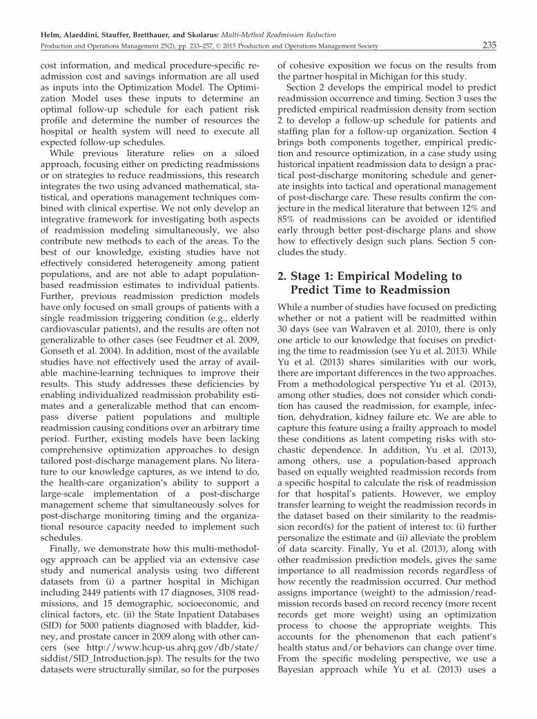
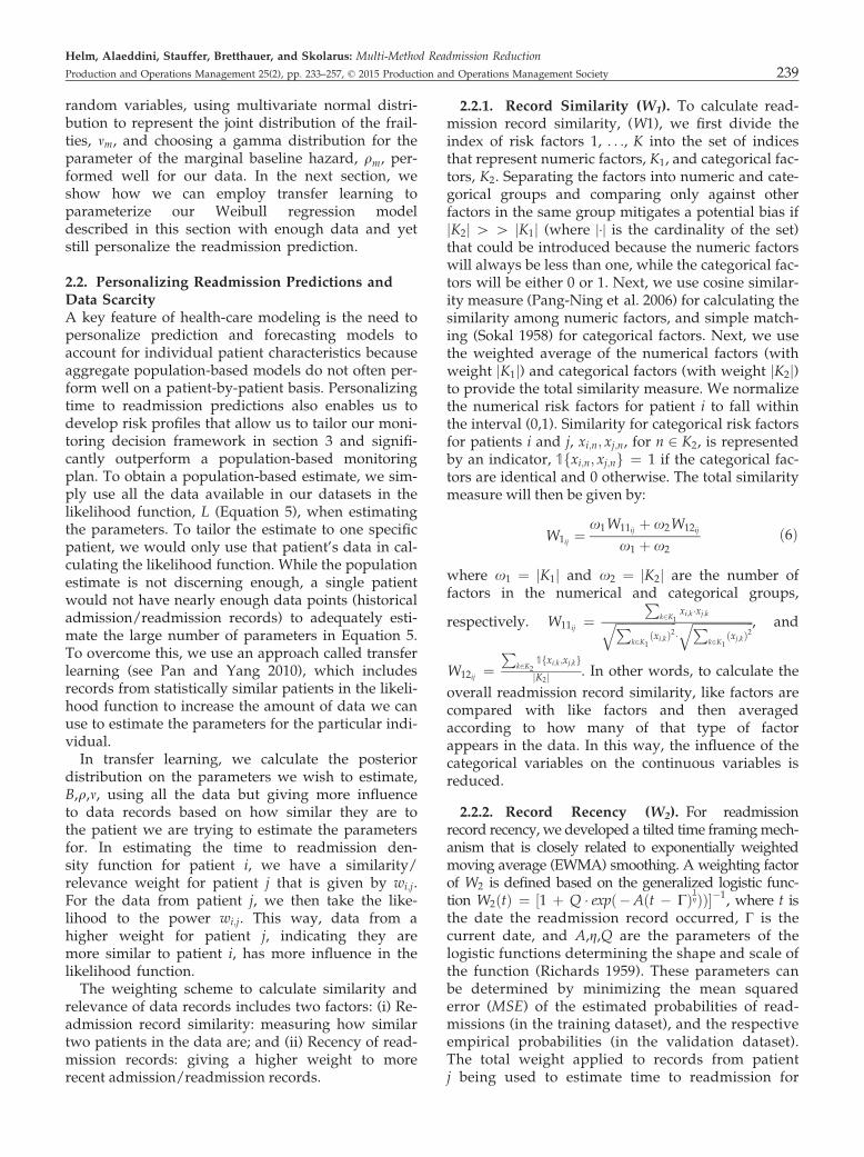
case simulated annealing) to determine the optimalvalue of the parameters for the weight function,W2ðtÞ, based on the validation dataset. The objectivefunction of the simulated annealing algorithm wastaken as the MSE of the estimated probabilities of re-admission for patients in the validation set using themodel parameterized in the training dataset vs. therespective empirical probabilities in the validationdataset. However, weighting parameters complicatethe likelihood function and consequently affect theefficiency of the Bayesian updating procedure. Todeal with this, we employ a simple, yet effective tech-nique of replicating admission/readmission recordsbased on their weights. For example, if there are tworecords where one of them has weight two, while theother is a regular record with weight one, we mayreplicate the first one twice and leave the last onewithout replication. The appropriate number of repli-cations for each record in more complex scenarios canbe achieved by using the least common multiple ofthe weights.Figure 3 presents the MSE in predicting individual

patient’s probability of readmission based on applica-tion to the testing data in the threefold cross-valida-tion using approximately 620 records (20% of the total3108 readmission records). Four time snapshots (30,60, 180, and 360 days after discharge) were used to

Table 1 High-Level Procedure of the Readmission PredictionFramework

Readmission prediction procedure

Input Readmission data, Prior dist. of hazard functionparameters and risk factor covariates

Output Posterior dist. of hazard function parametersand risk factor covariates

Empirical time to readmission density functionProcedure 1. Set prior dist. for risk factors, frailties, and marginal

baseline hazard (e.g., double exponential,multivariate normal, gamma)

2. Set W2 function parameters (record recency weight)3. FOR patient i in dataset4. Calculate the total weight of all records in

the database with respect to the last readmissionevent of patient i

5. Replicate each record according to the leastcommon multiplier of the calculated weights

6. Find the posterior distribution of the modelparameters based on the weighted datasetusing Gibbs sampling

7. Calculate the posterior distribution of readmission/no readmission based on optimal parametersNEXT PATIENT

Return Posteriors


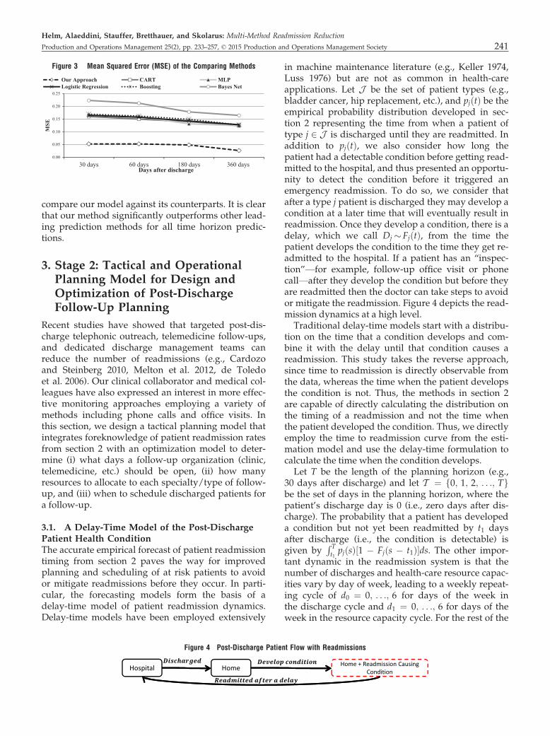
compare our model against its counterparts. It is clearthat our method significantly outperforms other lead-ing prediction methods for all time horizon predic-tions.

3. Stage 2: Tactical and OperationalPlanning Model for Design andOptimization of Post-DischargeFollow-Up Planning

Recent studies have showed that targeted post-dis-charge telephonic outreach, telemedicine follow-ups,and dedicated discharge management teams canreduce the number of readmissions (e.g., Cardozoand Steinberg 2010, Melton et al. 2012, de Toledoet al. 2006). Our clinical collaborator and medical col-leagues have also expressed an interest in more effec-tive monitoring approaches employing a variety ofmethods including phone calls and office visits. Inthis section, we design a tactical planning model thatintegrates foreknowledge of patient readmission ratesfrom section 2 with an optimization model to deter-mine (i) what days a follow-up organization (clinic,telemedicine, etc.) should be open, (ii) how manyresources to allocate to each specialty/type of follow-up, and (iii) when to schedule discharged patients fora follow-up.

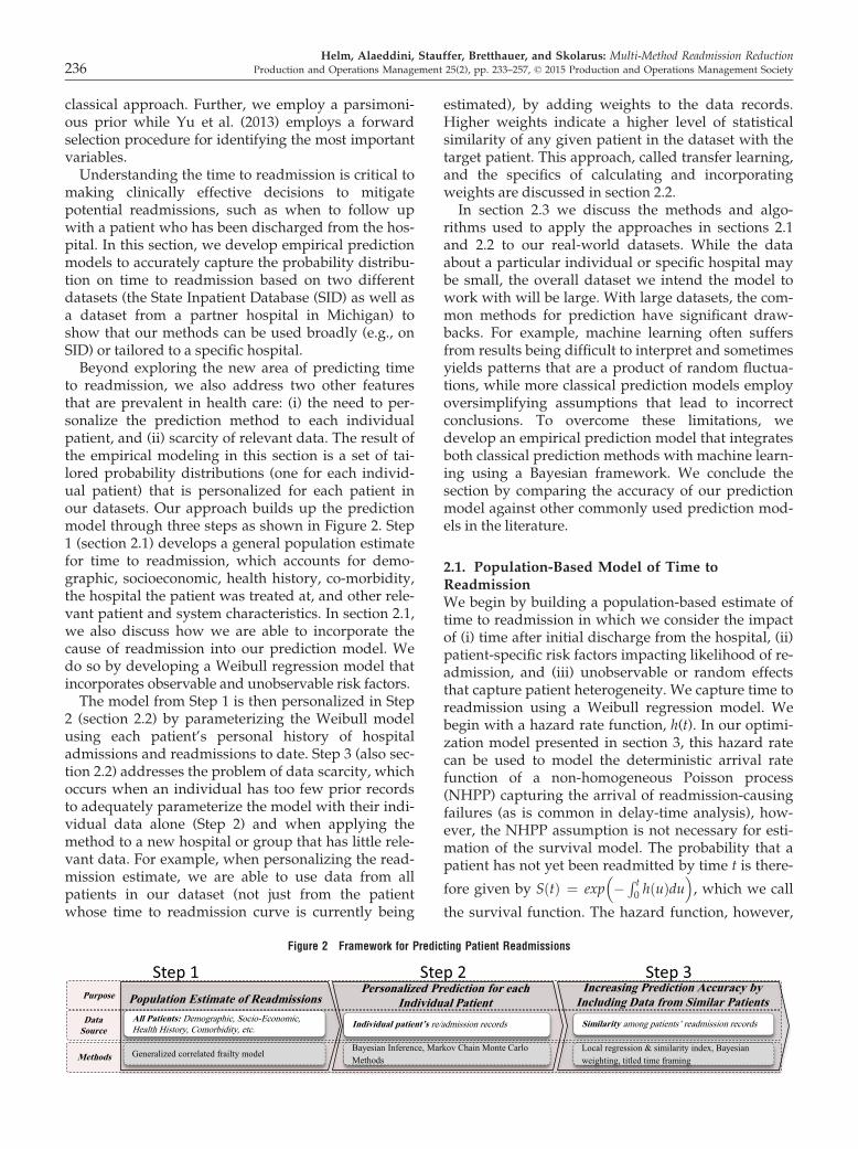
3.1. A Delay-Time Model of the Post-DischargePatient Health ConditionThe accurate empirical forecast of patient readmissiontiming from section 2 paves the way for improvedplanning and scheduling of at risk patients to avoidor mitigate readmissions before they occur. In parti-cular, the forecasting models form the basis of adelay-time model of patient readmission dynamics.Delay-time models have been employed extensively

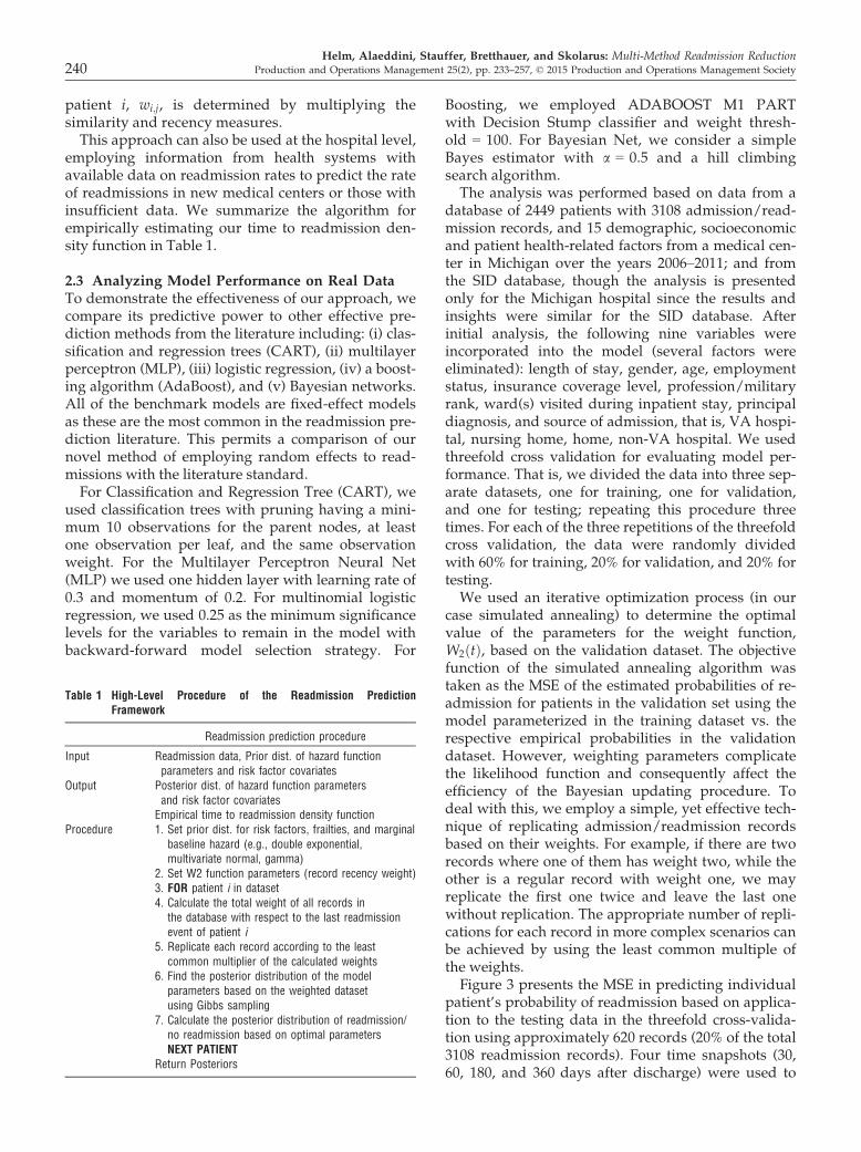
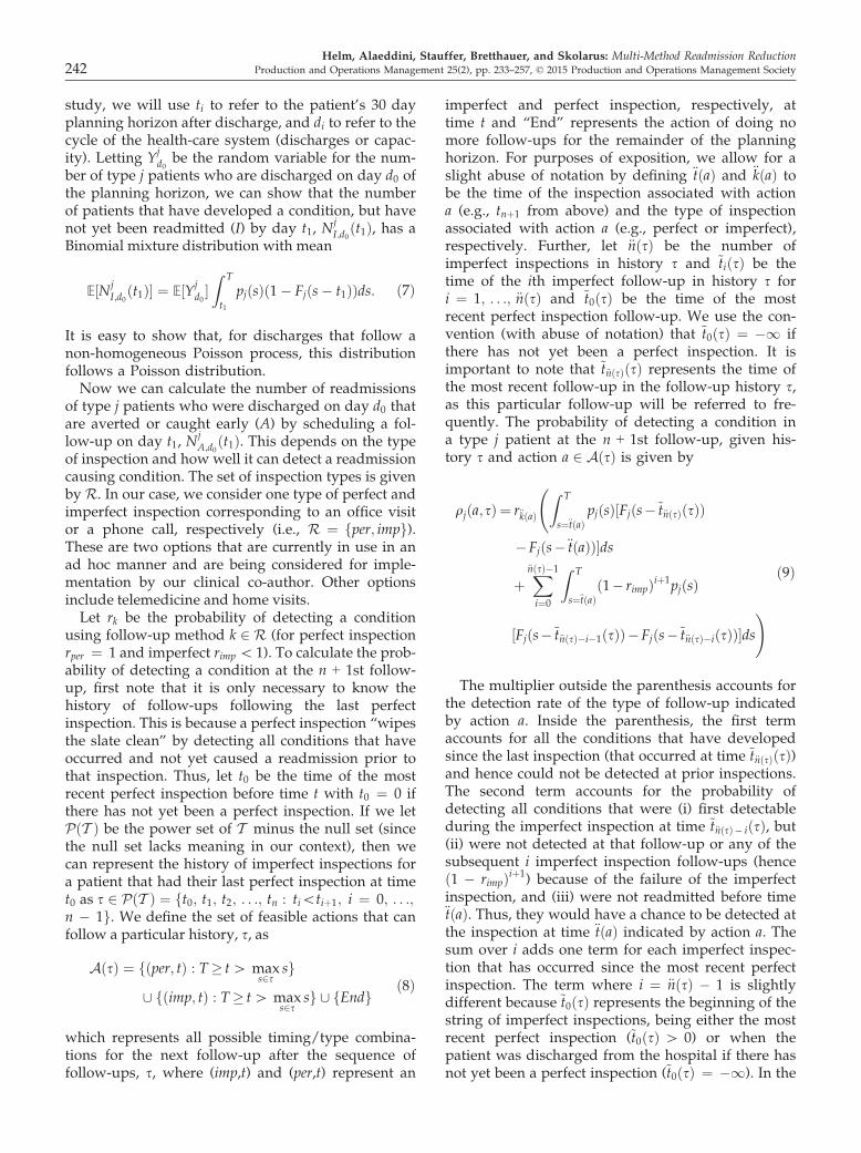
in machine maintenance literature (e.g., Keller 1974,Luss 1976) but are not as common in health-careapplications. Let J be the set of patient types (e.g.,bladder cancer, hip replacement, etc.), and pjðtÞ be theempirical probability distribution developed in sec-tion 2 representing the time from when a patient oftype j 2 J is discharged until they are readmitted. Inaddition to pjðtÞ, we also consider how long thepatient had a detectable condition before getting read-mitted to the hospital, and thus presented an opportu-nity to detect the condition before it triggered anemergency readmission. To do so, we consider thatafter a type j patient is discharged they may develop acondition at a later time that will eventually result inreadmission. Once they develop a condition, there is adelay, which we call Dj � FjðtÞ, from the time thepatient develops the condition to the time they get re-admitted to the hospital. If a patient has an “inspec-tion”—for example, follow-up office visit or phonecall—after they develop the condition but before theyare readmitted then the doctor can take steps to avoidor mitigate the readmission. Figure 4 depicts the read-mission dynamics at a high level.Traditional delay-time models start with a distribu-

tion on the time that a condition develops and com-bine it with the delay until that condition causes areadmission. This study takes the reverse approach,since time to readmission is directly observable fromthe data, whereas the time when the patient developsthe condition is not. Thus, the methods in section 2are capable of directly calculating the distribution onthe timing of a readmission and not the time whenthe patient developed the condition. Thus, we directlyemploy the time to readmission curve from the esti-mation model and use the delay-time formulation tocalculate the time when the condition develops.Let T be the length of the planning horizon (e.g.,

30 days after discharge) and let T ¼ f0; 1; 2; . . .; Tgbe the set of days in the planning horizon, where thepatient’s discharge day is 0 (i.e., zero days after dis-charge). The probability that a patient has developeda condition but not yet been readmitted by t1 daysafter discharge (i.e., the condition is detectable) isgiven by

R Tt1pjðsÞ½1 � Fjðs � t1Þ�ds. The other impor-

tant dynamic in the readmission system is that thenumber of discharges and health-care resource capac-ities vary by day of week, leading to a weekly repeat-ing cycle of d0 ¼ 0; . . .; 6 for days of the week inthe discharge cycle and d1 ¼ 0; . . .; 6 for days of theweek in the resource capacity cycle. For the rest of the

0.00

0.05

0.10

0.15

0.20

0.25

30 days 60 days 180 days 360 days

MSE

Days after discharge

Our Approach CART MLPLogistic Regression Boosting Bayes Net

Figure 3 Mean Squared Error (MSE) of the Comparing Methods

Hospital Home Home + Readmission CausingCondition

Figure 4 Post-Discharge Patient Flow with Readmissions



study, we will use ti to refer to the patient’s 30 dayplanning horizon after discharge, and di to refer to thecycle of the health-care system (discharges or capac-ity). Letting Y

jd0

be the random variable for the num-ber of type j patients who are discharged on day d0 ofthe planning horizon, we can show that the numberof patients that have developed a condition, but havenot yet been readmitted (I) by day t1, N

jI;d0

ðt1Þ, has aBinomial mixture distribution with mean

E½NjI;d0

ðt1Þ� ¼ E½Yjd0�Z T

t1

pjðsÞð1� Fjðs� t1ÞÞds: ð7Þ

It is easy to show that, for discharges that follow anon-homogeneous Poisson process, this distributionfollows a Poisson distribution.Now we can calculate the number of readmissions

of type j patients who were discharged on day d0 thatare averted or caught early (A) by scheduling a fol-low-up on day t1, N

jA;d0

ðt1Þ. This depends on the typeof inspection and how well it can detect a readmissioncausing condition. The set of inspection types is givenby R. In our case, we consider one type of perfect andimperfect inspection corresponding to an office visitor a phone call, respectively (i.e., R ¼ fper; impg).These are two options that are currently in use in anad hoc manner and are being considered for imple-mentation by our clinical co-author. Other optionsinclude telemedicine and home visits.Let rk be the probability of detecting a condition

using follow-up method k 2 R (for perfect inspectionrper ¼ 1 and imperfect rimp \ 1). To calculate the prob-ability of detecting a condition at the n + 1st follow-up, first note that it is only necessary to know thehistory of follow-ups following the last perfectinspection. This is because a perfect inspection “wipesthe slate clean” by detecting all conditions that haveoccurred and not yet caused a readmission prior tothat inspection. Thus, let t0 be the time of the mostrecent perfect inspection before time t with t0 ¼ 0 ifthere has not yet been a perfect inspection. If we letPðT Þ be the power set of T minus the null set (sincethe null set lacks meaning in our context), then wecan represent the history of imperfect inspections fora patient that had their last perfect inspection at timet0 as s 2 PðT Þ ¼ ft0; t1; t2; . . .; tn : ti\tiþ1; i ¼ 0; . . .;n � 1g. We define the set of feasible actions that canfollow a particular history, s, as

AðsÞ ¼ fðper; tÞ : T� t[ maxs2s

sg

[ fðimp; tÞ : T� t[ maxs2s

sg [ fEndgð8Þ

which represents all possible timing/type combina-tions for the next follow-up after the sequence offollow-ups, s, where (imp,t) and (per,t) represent an

imperfect and perfect inspection, respectively, attime t and “End” represents the action of doing nomore follow-ups for the remainder of the planninghorizon. For purposes of exposition, we allow for aslight abuse of notation by defining €tðaÞ and €kðaÞ tobe the time of the inspection associated with actiona (e.g., tnþ1 from above) and the type of inspectionassociated with action a (e.g., perfect or imperfect),respectively. Further, let €nðsÞ be the number ofimperfect inspections in history s and ~tiðsÞ be thetime of the ith imperfect follow-up in history s fori ¼ 1; . . .; €nðsÞ and ~t0ðsÞ be the time of the mostrecent perfect inspection follow-up. We use the con-vention (with abuse of notation) that ~t0ðsÞ ¼ �1 ifthere has not yet been a perfect inspection. It isimportant to note that ~t€nðsÞðsÞ represents the time ofthe most recent follow-up in the follow-up history s,as this particular follow-up will be referred to fre-quently. The probability of detecting a condition ina type j patient at the n + 1st follow-up, given his-tory s and action a 2 AðsÞ is given by

qjða;sÞ ¼ r€kðaÞ

Z T

s¼€tðaÞpjðsÞ½Fjðs�~t€nðsÞðsÞÞ

�Fjðs�€tðaÞÞ�ds

þX€nðsÞ�1

i¼0

Z T

s¼€tðaÞð1� rimpÞiþ1pjðsÞ

½Fjðs�~t€nðsÞ�i�1ðsÞÞ�Fjðs�~t€nðsÞ�iðsÞÞ�ds!

ð9Þ

The multiplier outside the parenthesis accounts forthe detection rate of the type of follow-up indicatedby action a. Inside the parenthesis, the first termaccounts for all the conditions that have developedsince the last inspection (that occurred at time ~t€nðsÞðsÞ)and hence could not be detected at prior inspections.The second term accounts for the probability ofdetecting all conditions that were (i) first detectableduring the imperfect inspection at time ~t€nðsÞ� iðsÞ, but(ii) were not detected at that follow-up or any of thesubsequent i imperfect inspection follow-ups (henceð1 � rimpÞiþ1) because of the failure of the imperfectinspection, and (iii) were not readmitted before time€tðaÞ. Thus, they would have a chance to be detected atthe inspection at time €tðaÞ indicated by action a. Thesum over i adds one term for each imperfect inspec-tion that has occurred since the most recent perfectinspection. The term where i ¼ €nðsÞ � 1 is slightlydifferent because ~t0ðsÞ represents the beginning of thestring of imperfect inspections, being either the mostrecent perfect inspection (~t0ðsÞ [ 0) or when thepatient was discharged from the hospital if there hasnot yet been a perfect inspection (~t0ðsÞ ¼ �1). In the


case where ~t0ðsÞ ¼ �1 (no perfect inspection yet),then Fjðs � ~t0ðsÞÞ ¼ 1, which corresponds to the factthat failures only begin to arrive after the patient isdischarged (since the discharge process is considereda perfect inspection). Thus, 1 � Fjðs � ~t1ðsÞÞ repre-sents conditions that were first detectable at the firstimperfect inspection and have not yet caused a read-mission.Equation 9 gives the probability of detecting a read-

mission causing condition for an individual patient.We now link this detection probability to the decisionof how many appointment slots to reserve for follow-ing up with a cohort of patients that are dischargedfrom the hospital. With a 2 AðsÞ being the timing andtype of the next follow-up we define this decision var-iable as Hj;a

d0;s, which is the number of phone call slots

(if €kðaÞ ¼ imp) or office visit appointments (if€kðaÞ ¼ per) to reserve on day €tðaÞ for type j 2 Jpatients who were discharged on day d0 ¼ 0; . . .; 6and have a follow-up history of s 2 PðT Þ. Eachfollow-up has the opportunity of detecting a condi-tion before it causes an emergency readmission. Theresult may still be a readmission, but a less costlyone. Our assumption is that detecting the conditionbefore it becomes an emergency readmission avertssome or all of the cost of an emergency readmissionfor that patient. This is what we mean by averting areadmission. Letting 1 be the indicator function, andrecalling that Y

jd0

is the number of patients of typej discharged on day d0, the number of additionalreadmissions averted by appointment allocationHj;a

d0;sis given by

NHj;a

d0 ;s

A;j ¼XY

j

d0^Hj;a

d0 ;s

‘¼1

1fCondition Detected at time

tnþ1 for Patient ‘g;

ð10Þ

where ^ represents the minimum operator. Asbefore, this also follows a Binomial mixture, whichcan be seen by conditioning on Y

jd0

and applying thelaw of total probability. Further, it can be shownthat

E½NHj;a

d0 ;s

A;j � ¼ E Yjd0^Hj;a

d0;s

h iqjða; sÞ ð11Þ

Because the Θ’s capture both the follow-up day,€tðaÞ, and the discharge day, d0, the optimization willreveal not only the capacity to allocate to follow-upson each day d1 ¼ 0; . . .; 6 (by summing the decisionvariable over f€tðaÞ : ð€tðaÞ þ d0Þmod 7 ¼ d1g) butalso the optimal timing of each follow-up for a patientof type j determined by the history s for all non-zeroΘ’s. The following sections will analyze the mix andvolume of follow-up types to determine how these

different methods (e.g., phone, office visit, etc.) can beused most effectively in practice. The goal is (i) todevelop an optimization model that identifies optimalplacement of both types of follow-up, (ii) understandthe structure of the placement of these follow-ups toprovide heuristics or rules of thumb that could beemployed in designing post-discharge follow-upplans even in the absence of optimization.

3.2. Optimal Design of a Post-DischargeMonitoring OrganizationWhile there is a rich literature on delay-time modelsin machine maintenance, the optimization model wedevelop adds new system-level decision-makingcapability not previously considered by allowing theoptimization to consider not only the timing ofinspections but also how much capacity to reserve forthose inspections over a planning horizon. Adding tothe complexity, each day has a stochastic number ofdischarges (potential patients to follow up with) witha different distribution for each day of the week aswell as a different cost for scheduling follow-ups byday of week. Finally, we develop a complex cyclosta-tionary equilibrium model with parameters varyingover a seven-day horizon, but allowing patients to bescheduled for inspection up to 30 days after their dis-charge. Next, we present the notation followed by themodel formulation.Let c

j;kd1

be the cost per appointment of type k 2 Rfor patient type j on day d1 ¼ 0; . . .; 6 (i.e., Sun-Sat).uj;a is the usage requirement of follow-up resourceindicated by action a 2 s for a type j patient (e.g.,some patients need 15-minute slots, whereas othersrequire 20- or 30-minute slots). bj is the average bene-fit of averting a readmission by early detection for atype j patient. Let ~Cd1;k be the maximum capacity of atype k follow-up resource that can be reserved on dayd1. To capture the cyclically time-varying cost ofreserving capacity for follow-ups, we define a func-tion that maps the follow-up day, t (on the scale of T ),after a discharge on day d0 2 f0; . . .; 6g, to the day ofweek the appointment would occur and correspond-ing cost:

cjða; d0Þ ¼ cj;€kðaÞðd0þ€tðaÞÞmod7

: ð12Þ

Finally, we need notation to capture the day of theweek that capacity is being reserved on toaccount for the costs that differ by day. LetMðd0; d1Þ ¼ ft 2 T : ðt þ d0Þmod 7 ¼ d1g be theset of possible follow-up days of a patient dis-charged on day d0 that map to the same day of theweek, d1. In this set, d0 is that day of the week ofdischarge (e.g., d0 ¼ 0 represents a Sunday dis-charge, . . .; d0 ¼ 6 represents a Saturday discharge)and t þ d0 represents the (relative) date t days after



discharge. Therefore, ðd0 þ €tðaÞÞmod 7 returns theday of the week for that date that is t days after thepatient’s discharge. d1 2 f0; . . .; 6g represents a dayof the week (e.g., d1 ¼ 1 is Monday), so ifðt þ d0Þmod 7 ¼ d1, then this implies that t daysafter discharge day d0 (e.g., Friday) is the d1 (e.g.,Monday) day of the week. Thus, Mðd0; d1Þ is all thedays within the planning horizon (e.g., t = 1, . . ., 30)that correspond to the day of week d1. For example,if d0 ¼ 5 (i.e., Friday) and d1 ¼ 1 (i.e., Monday),Mðd0; d1Þ ¼ f3; 10; 17; 24g as 3 days after Friday isMonday, 10 days after Friday is also Monday, etc.PROGRAM 1 provides an optimal design for staff-ing and scheduling of a follow-up organization.

PROGRAM 1:

minH

EXj2J

X6d0¼0

Xs2PðT Þ

Xa2AðsÞ

cjða; d0ÞHj;ad0;s

� uj;a � bjNHj;a

d0 ;s

A;j

24

35

ð13Þ

s.t.

~Cd1;k �Xj2J

X6d0¼0

Xs2PðT Þ

Xa2AðsÞ:€kðaÞ¼k;€tðaÞ2Mðd0;d1Þ

Hj;ad0;s

� uj;a

8d1 2 f0; . . .; 6g; k 2 Rð14Þ

Xa2AðsÞ

Hj;ad0;s

�Hj;ðimp;~t€nðsÞðsÞÞd0;snfðimp;~t€nðsÞðsÞÞg

8j 2 J ; d0 ¼ 0; . . .; 6; s 2 PðsÞ : jsj[ 1

ð15Þ

Xs2PðsÞ:~t€nðsÞ\t1

Hj;ðper;t1Þd0;s

�Xk2R

XTt2¼t1þ1

Hj;ðk;t2Þd0;ft1g

8j 2 J ; d0 ¼ 0; . . .; 6; t1 ¼ 2; . . .;T � 1

ð16Þ

The objective function minimizes the cost of staffingthe follow-up clinic minus the cost of readmissionsaverted. Equation 14 ensures that capacity con-straints for each resource are respected. This is com-plicated by the fact that we are considering a systemthat functions on a weekly repeating cycle. Thus, wehave different costs and discharge distributions foreach day of the week, but the pattern repeats eachweek. However, patient health status does notevolve on a weekly repeating cycle but instead playsout over a longer (non-repeating) horizon, which wedenote by T and can be thought of as the 30-day re-admission window for example. In order to ensurethat enough capacity is allocated on a given day ofthe week, take Monday, for example, we mustaccount for patients that are scheduled the firstMonday after their discharge, as well as those that

will be scheduled the second Monday after their dis-charge, and the third Monday after their dischargeand so forth. This is the reason for choosing the fol-low-up day such that ð€tðaÞ þ d0Þmod 7 is equal tothe day whose capacity is the focus of the constraint.We also consider all patients who were dischargedon different days of the week (the sum over d0)since the discharges vary by day of week in thecyclostationary health-care system.Finally, Equations 15 and 16 are critical constraints

linking sequential follow-ups together, ensuring thatthe follow-up time sequence follows the correct pattern.In particular, it should only be possible to schedule asmany follow-ups at time t1 in the sequence s [ ft1g asthe most follow-ups that were scheduled in any previ-ous visit in s. This is because the probability of detectionfor each patient is dependent on all the previous inspec-tion times, and so to obtain the correct detection proba-bility it is necessary that each patient being scheduledin a particular time sequence has taken every visit inthe sequence. Equation 15 ensures that the number ofinspections scheduled following a history s (LHS of theequation) is no more than the number of inspectionsscheduled in the most recent imperfect inspection in s(RHS of the equation). Equation 16 ensures the same forperfect inspections. The reason we need two separateconstraints to capture this criterion is because a perfectinspection “resets” the inspection history, and thusmust be treated differently.The stochastic optimization model in PROGRAM 1

suffers from an extremely large state space, actionspace, and number of constraints. Both the number ofdecision variables and number of constraints in Equa-tion 16 are exponential in the length of the planninghorizon because the probability of detection at eachvisit depends on the history of all imperfect inspec-tions since the last perfect inspection. Further, the factthat the number of discharges on a given day can be

stochastic makes E½NHj;a

d0 ;s

A;j � a non-linear function of the

decision variable,Hj;ad0;s

.

3.2.1. Computational Challenges. It is easy to seethat the number of constraints represented by Equa-tion 15 is exponential because of PðT Þ. Proposition 1shows that the number of decision variables in PRO-GRAM 1 is also exponential in the length of the plan-ning horizon.

PROPOSITION 1. Let T be the length of the planning hori-zon. The number of decision variables in PROGRAM 1is jJ jjRj � 7ð2Tþ1 � ðT þ 2ÞÞ.

PROOF. At each time point, t, in the planning hori-zon there are two choices: schedule a perfect inspec-tion or an imperfect inspection. The outcome of the


choice depends on the history of imperfect inspec-tions and the time of the most recent perfect inspec-tion prior to t. If the last perfect inspection were attime t � 1, there is only one possible history (i.e.,20) that has an inspection at time t. If the last perfectwas at time t � 2, there are two possible (i.e., 21)histories per, imp or per, None. If the last perfectinspection was at time s then there are 2t� s� 1 possi-ble histories. If there was no previous perfect inspec-tion, there are 2t�1 histories. Thus, at time t, thereare a total of

Pt� 1s¼ 0 2

s ¼ 2t � 1 possible historiesand there are jRj possible actions at time t (inour case jRj ¼ 2: perfect or imperfect inspection).Thus, there are jRjð2t � 1Þ decision variables attime t. Summing this over all time points in the plan-

ning horizon yields jRjPT

t¼0ð2t � 1Þ ¼ jRjð2Tþ1 �ðT þ 2Þ. Finally, this pattern repeats for each patienttype (of which there are jJ j) and days in the cost/discharge cycle (d = 0, . . ., 6). h

For a 30-day planning horizon, the number of deci-sion variables significantly exceeds commercial solverlimits. To handle the problem size, we introduce anew, network flow-based method for transformingthe stochastic optimization problem into a tractablelinear deterministic one in the next section. We showthat this transformed problem is actually a weaklycoupled network flow problem (defined in section3.3), which can be decomposed into several indepen-dent networks with a few linking constraints. Notonly does the network flow formulation allow formuch faster solution approaches, the network flowstructure inherently captures constraints of Equations15 and 16, leaving only a small number of linking con-straints (Equation 14) that weakly couple otherwiseindependent networks for each patient type and dayof week.Finally, by applying pruning methods to our

decomposed network models, we are able to solveeven large problems very effectively. This allows usto design complete patient follow-up monitoringschedules as well as staffing plans for a realisticallysized follow-up organization. The development ofsuch techniques has the potential to impact manyareas by providing a methodology for solving multi-dimensional, large state space stochastic optimizationproblems that are common to the health-care domainand elsewhere.

3.3. Network Flow-Based Transformation of theStochastic Optimization ModelMethods in the literature have been developed fortransforming these stochastic queueing networkproblems into deterministic ones that admit tractableoptimization methods. Unfortunately, prior transfor-mations in this vein of literature (such as Helm and

Van Oyen 2014, Helm et al. 2013, and Deglise-Hawkinson et al. 2013) fail when applied to solvereasonably sized post-discharge monitoring problems.After applying previous transformation methods,we could solve problems in a reasonable time for a15-day planning horizon, as shown in Figure 6,whereas our goal is to develop an optimal schedule toreduce 30-day readmissions.In this section, we show that our problem has a spe-

cial structure that allows us to decompose our prob-lem into a set of independent network flow modelswith a small number of linking side constraints. Simi-lar to the naming convention of Gocgun and Ghate(2012), we call this a weakly coupled network flowproblem. We develop methods to solve large problemsizes that are intractable for general linear program-ming representations of the readmission problem thatdo not exploit the weakly coupled network structure.Our particular model of post-discharge monitoringexploits the fact that we can decompose the monitor-ing problem along days of the repeating dischargeand follow-up cost cycle (e.g., days of the week),along patient types, and along probabilistic samplepaths in the case of stochastic discharges. If there aren patient types and a maximum of m possible dis-charges on any given day then we would solve 7�m�nsmaller networks (each of which typically solves inseconds) instead of one large network (that is toolarge to input into commercial solvers). UsingLagrangian relaxation on the linking constraints, wecan decouple these 7�m�n networks and solve them inparallel, allowing for much larger problems to besolved. In fact, we are able to solve the 30-day horizonproblem relatively quickly, even though the numberof potential decisions is extremely large.We first present the network model with determin-

istic discharges and then extend the model to incorpo-rate stochastic discharges. To do so, we show that thenon-linear stochastic objective, the expected numberof readmissions averted for any given capacity limit

(i.e., E Yjd0^Hj;a

d0;s

h ifrom Equation 11), can be calcu-

lated exactly using a new stochastic branchingmethod that we develop. This method maintains theweakly coupled network structure and allows us todecompose the problem and tractably solve a set ofsmaller network flows with side constraints. A furtherconvenient feature of our stochastic branchingmethod is that the number of “stochastic” branchestaken determines the optimal amount of capacity toreserve on each day.

3.3.1. Deterministic Discharges. We begin bydescribing the individual decoupled networks, onefor each discharge day and patient type, whichare the building blocks of the full, weakly coupled



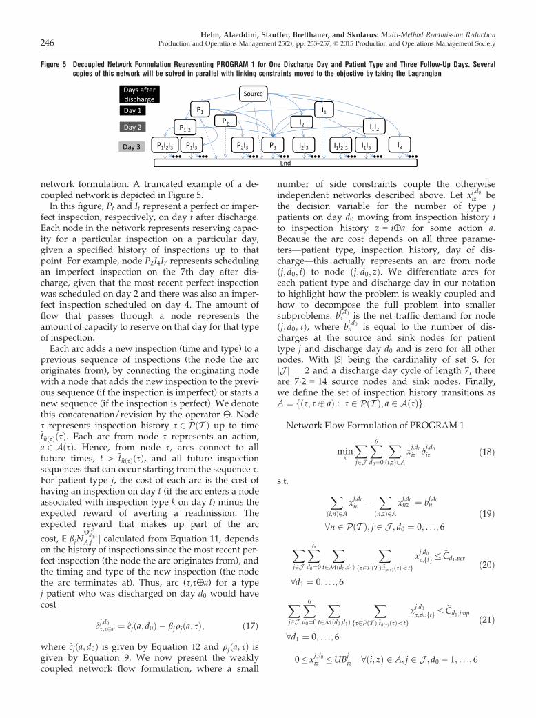
network formulation. A truncated example of a de-coupled network is depicted in Figure 5.In this figure, Pt and It represent a perfect or imper-

fect inspection, respectively, on day t after discharge.Each node in the network represents reserving capac-ity for a particular inspection on a particular day,given a specified history of inspections up to thatpoint. For example, node P2I4I7 represents schedulingan imperfect inspection on the 7th day after dis-charge, given that the most recent perfect inspectionwas scheduled on day 2 and there was also an imper-fect inspection scheduled on day 4. The amount offlow that passes through a node represents theamount of capacity to reserve on that day for that typeof inspection.Each arc adds a new inspection (time and type) to a

previous sequence of inspections (the node the arcoriginates from), by connecting the originating nodewith a node that adds the new inspection to the previ-ous sequence (if the inspection is imperfect) or starts anew sequence (if the inspection is perfect). We denotethis concatenation/revision by the operator ⊕. Nodes represents inspection history s 2 PðT Þ up to time~t€nðsÞðsÞ. Each arc from node s represents an action,a 2 AðsÞ. Hence, from node s, arcs connect to allfuture times, t [ ~t€nðsÞðsÞ, and all future inspectionsequences that can occur starting from the sequence s.For patient type j, the cost of each arc is the cost ofhaving an inspection on day t (if the arc enters a nodeassociated with inspection type k on day t) minus theexpected reward of averting a readmission. Theexpected reward that makes up part of the arc

cost, E½bjNHj;a

d0 ;s

A;j � calculated from Equation 11, dependson the history of inspections since the most recent per-fect inspection (the node the arc originates from), andthe timing and type of the new inspection (the nodethe arc terminates at). Thus, arc (s,s⊕a) for a typej patient who was discharged on day d0 would havecost

dj;d0s;sa ¼ cjða; d0Þ � bjqjða; sÞ; ð17Þ

where cjða; d0Þ is given by Equation 12 and qjða; sÞ isgiven by Equation 9. We now present the weaklycoupled network flow formulation, where a small

number of side constraints couple the otherwiseindependent networks described above. Let x

j;d0iz be

the decision variable for the number of type jpatients on day d0 moving from inspection history ito inspection history z = i⊕a for some action a.Because the arc cost depends on all three parame-ters—patient type, inspection history, day of dis-charge—this actually represents an arc from nodeðj; d0; iÞ to node ðj; d0; zÞ. We differentiate arcs foreach patient type and discharge day in our notationto highlight how the problem is weakly coupled andhow to decompose the full problem into smallersubproblems. b

j;d0s is the net traffic demand for node

ðj; d0; sÞ, where bj;d0n is equal to the number of dis-

charges at the source and sink nodes for patienttype j and discharge day d0 and is zero for all othernodes. With |S| being the cardinality of set S, forjJ j ¼ 2 and a discharge day cycle of length 7, thereare 7�2 = 14 source nodes and sink nodes. Finally,we define the set of inspection history transitions asA ¼ fðs; s aÞ : s 2 PðT Þ; a 2 AðsÞg.

Network Flow Formulation of PROGRAM 1

minx

Xj2J

X6d0¼0

Xði;zÞ2A

xj;d0iz dj;d0iz ð18Þ

s.t. Xði;nÞ2A

xj;d0in �

Xðn;zÞ2A

xj;d0nz ¼ b

j;d0n

8n 2 PðT Þ; j 2 J ; d0 ¼ 0; . . .; 6

ð19Þ

Xj2J

X6d0¼0

Xt2Mðd0;d1Þ

Xfs2PðT Þ:~t€nðsÞðsÞ\tg

xj;d0s;ftg � ~Cd1;per

8d1 ¼ 0; . . .; 6

ð20Þ

Xj2J

X6d0¼0

Xt2Mðd0;d1Þ

Xfs2PðT Þ:~t€nðsÞðsÞ\tg

xj;d0s;s[ftg � ~Cd1;imp

8d1 ¼ 0; . . .; 6

ð21Þ

0� xj;d0iz �UB

jiz 8ði; zÞ 2 A; j 2 J ; d0 � 1; . . .; 6

I1

P2 I1I2

P1

I2P1I2

Source

P3 I2I3 I3P2I3P1I2I3 I1I2I3P1I3 I1I3

End

Day 1

Day 2

Day 3

Days afterdischarge

Figure 5 Decoupled Network Formulation Representing PROGRAM 1 for One Discharge Day and Patient Type and Three Follow-Up Days. Severalcopies of this network will be solved in parallel with linking constraints moved to the objective by taking the Lagrangian


Equation 18 is the objective, which is a min-costflow. Equation 19 is the flow conservation con-straint. Equation 20 is the capacity constraint forperfect inspections. Every time there is a perfectinspection at time t, it wipes the information setclean except for the perfect inspection at time t.Hence, the arc x

j;d0s;ftg represents a perfect inspection

at time t given a history of s. t is chosen so that itfalls on day of the week d1 (see the sum overt 2 Mðd0; d1Þ. To capture every possible perfectinspection at time t, we also sum over all possibleimperfect inspection histories in which all theinspections occur before t, given by fs 2 PðT Þ :~t€nðsÞðsÞ\ tg, and recalling that ~t€nðsÞðsÞ is the mostrecent inspection (largest inspection time) in s.Finally, there is a sum over all possible dischargedays, d0, since patients discharged on any of thedischarge days in the cycle may be scheduled forday d1 and use up some of the capacity. Equation21 accomplishes the same purpose except forimperfect inspections. All components are thesame as Equation 20, except in the index of thedecision variable, the information set is changed byappending the new inspection at time t to the for-mer history s; hence the arc x

j;d0s;s[ftg goes from

inspection history s to inspection history s∪{t}instead of erasing the old history as with theperfect inspection.

3.3.1.1. Side Constraint Elimination and NetworkDecomposition: Next, we discuss an efficient solutionmethod that is capable of solving large-scaleinstances of the weakly coupled Network FlowFormulation of PROGRAM 1. Inspection of theproblem structure reveals that the constraint set isblock diagonal, with the blocks linked together by arelatively small number of the system capacity con-straints defined in Equation 20 and 21. Further, eachblock is an independent set of network flow con-straints. Fortunately, there are only a few of theseside constraints relative to the number of constraintsthat fit the network flow structure. By taking theLagrangian relaxation of these constraints it is possi-ble to iteratively solve pure network problems anduse the subgradient method until the algorithm con-verges to an acceptable tolerance (see Fisher 1985,Geoffrion 1974). Further, Equations 20 and 21 arethe only constraints that link patient types and dis-charge days to one another because of the sum overj 2 J and d0 ¼ 0; . . .; 6. Once these constraints aretaken into the objective function, the full networkproblem can now be decomposed into subproblemswith one pure network subproblem for each patienttype and discharge day. The subproblem looks thesame as the original except with a fixed j and d0 inEquation 19 and in the objective as well as theLagrangian of the side constraints.

By taking advantage of this problem structure, weare able to solve large-scale problems to optimality inmost cases, and near optimality in the remaining fewcases. Specifically, we relax the capacity constraintsEquations 20 and 21 into the objective function with acorresponding vector υ of Lagrange multipliers. Thevector υ has jRj � 7 elements (where in our casejRj ¼ 2, corresponding to perfect and imperfectinspection types), one multiplier per capacity con-straint in Equations 20 and 21. The resulting relaxedproblem then further decomposes into 7 � jJ j inde-pendent network flow subproblems, one for eachpatient type and discharge day of week, that can besolved very quickly using subgradient optimization(see Held et al. 1974) to search for the optimal multi-pliers.

3.3.2. Stochastic Discharges Network Model. Inthis section, we extend the deterministic model ofsection 3.3.1 to consider the case of a stochastic numberof patients being discharged from the hospital. Unfor-tunately, the presence of stochastic discharges not onlydestroys the network structure, but it also eliminatesthe linearity of the model. From the network stand-point, with deterministic discharges the number ofpatients scheduled was the same as the numberdischarged. With stochastic discharges, you must payfor the capacity reserved but you only get benefit forthe number of patients that actually get scheduled.Thus, the concept of arcs from the deterministic modelhas no meaning in the stochastic case because flowmeans something different for cost (amount of slotsreserved) and for benefit (number of patients seentimes benefit). The capacity reservation remains linearin amount of appointment slots reserved but fromEquation 11 the benefit from capacity reserved is

E Yjd0^ x

j;d0s;sa

h iqjða; sÞ ¼ qjða; sÞ

Xxj;d0s;sa

n¼0

PðYjd0� nÞ; ð22Þ

which is no longer linear, nor even convex. To over-come this challenge and restore both linearity andthe network structure, we employ a stochasticbranching method we call sample path decomposition.

3.3.2.1. Sample Path Decomposition: To incorporatestochastic discharges, we further decompose the net-work along sample path realizations and then sendexactly one unit of flow through each subproblem.Let xn be the realization of the discharge random var-iable Y

jd0that corresponds to the number of discharges

being larger than or equal to n. Thus,PðxnÞ ¼ PðYj

d0� nÞ. If the maximum possible num-

ber of discharges is M, then we decompose eachdeterministic subproblem (with a source supply ofbj;d00 � 1) into M subproblems with a source supply of



bj;d0;xn

0 ¼ 1 for n = 1, . . ., M. Then, the cost of each arc(similar to Equation 17) is given by

dj;d0;xn

s;sa ¼ cjða; d0Þ � bjPðxnÞqjða; sÞ; ð23Þ

Now xj;d0;xn

iz is the decision variable indicatingwhether the nth patient of type j discharged on day d0moves from inspection history i to inspection historyz = i⊕a for some action a. The objective becomesminx

Pj2JP6

d0¼0

PMn¼1

Pði;zÞ2A x

j;d0;xn

iz dj;d0;xn

iz . Note thisobjective calculates exactly the desired objective ofEquation 22. The flow balance constraints remain thesame except for an addition of the xn index to Equa-tion 19. Recall that the sample path decompositionnow defines flows as actual patients arriving to beseen rather than slots reserved, but it is necessary topay for all slots reserved, whether or not patients areseen. However, in each subproblem the full price ofcapacity is charged for each unit of flow sent acrossthe arc, but the benefit is discounted by the probabil-ity of the patient showing up, PðxnÞ.The final challenge is how to deal with capacity

constraints. Again the flows represent patients seen,but we must reconcile this with the fact that capacityconstraints refer to appointments reserved. This ishandled as follows. For the nth subproblem (xn), thesolution of the network flow subproblem will sendzero flow through a resource on a particular day(even if positive flow was sent at a xm for m < n),indicating that the probability that the nth patient willshow up is not worth the cost of reserving an appoint-ment for that patient. Thus, for each day of the plan-ning horizon (d1 ¼ 0; . . .; 6), let m be the last networkwith positive flow on that day. Then, m is the amountof capacity that should be reserved. Summing thebenefit from each network matches the definition ofthe objective in Equation 22, in which the LHS is thethe expected benefit from reserving x

j;d0s;sa capacity

and the RHS is exactly the calculation that we get bysumming the non-zero flows from the xm subprob-lems. The costs also match, since each flow is chargedthe full cost of the capacity reserved. Thus, the capac-ity calculation in the Lagrangian relaxation will becorrect as well.After applying the sample path decomposition, it is

now possible to regain linearity and the pure networkform while only increasing solution times linearly inM (the maximum possible discharges), althoughusing parallel computing solution times may notincrease at all. This is true because it is only necessaryto solve M additional subproblems (xi fori = 1, . . ., M) for each original subproblem from thedeterministic optimization and these subproblemscan be solved in parallel similar to the previouslydescribed decompositions. Using the pruning meth-ods developed in the next section, however, it will

become clear that in most cases it will not benecessary to solve anywhere near M subproblems toincorporate stochasticity as PðxiÞ will quickly becomeso small that all branches can be pruned, therebyeliminating the need to solve any xj for j > i.

3.3.3. Pruning Arcs/NodesEven with the weakly coupled network formulation,the size of the problem still hinders us from solving afull 30-day planning horizon as the number of arcsand nodes grows too large for commercial solvers.Computational results supporting this are presentedin section 3.3.4. Fortunately, the special structure ofour problem enables us to prune a large number ofarcs and nodes from the network without impactingthe optimal solution. The following theorem formal-izes this notion by guaranteeing that certain arcs willnever be taken in the optimal solution.

THEOREM 1. In the Network Flow Formulation of PRO-GRAM 1 (stochastic and deterministic), an arc withpositive cost will have zero flow in the optimal solutionto the network flow.

PROOF. We prove the result by showing that anysolution with a positive cost arc can be improved byredirecting the flow away from the arc. Thus, in anyoptimal solution no flow will be placed along posi-tive cost arcs. Consider such a solution where arcsðs1; s2Þ and ðs2; s3Þ both have non-zero flow and thecosts of arc ðs1; s2Þ is c12 [ 0 and the cost of arcðs2; s3Þ is c23 \ 0. If we send flow on arc ðs1; s2Þ andðs2; s3Þ along the arc ðs1; s3Þ instead we gain c1;2because we are no longer sending flow along thepositive arc. Further, the cost of arc ðs1; s3Þ is betterthan the cost of ðs2; s3Þ (i.e., c13 \ c23) becauseremoving the inspection in between the inspectionat s1 and the one at s3 only increases the value ofthe inspection at s3, since it is less likely that a pre-vious inspection has caught the potential readmis-sion. This can be seen directly from Equation 9.Also from Equation 9, the costs of all subsequentinspections after node s3 are also either improved ornot impacted because having one fewer inspectionin the history of inspections does not decrease thevalue of all subsequent inspections. Thus, redirect-ing the flow on the positive valued arc results in alower overall cost flow. h

Not only does Theorem 1 enable the pruning of alarge portion of the arcs and nodes for any given net-work, it also leads to the result that the optimal sche-dule of a longer planning horizon can often beobtained by solving a network for a much shorterplanning horizon. The following corollary states thisformally.


COROLLARY 1. Let Vj;d0

ðtÞ (deterministic) or Vj;d0;x

ðtÞ(stochastic) be the optimal value of subproblem of thenetwork flow formulation of Program 1 for type jpatients discharged on day d0 (with sample path x forstochastic) under a planning horizon of length t. S be

the time s.t. maxt [ S

fbjqjððper; tÞ; f0gÞ � cjððper; tÞ; d0Þg\ 0

(deterministic) or maxt [ S

fbjPðxÞqjððper; tÞ; f0gÞ�cjððper; tÞ; d0Þg\ 0 (stochastic). Then V

j;d0ðtÞ ¼ V

j;d0ðSÞ

(similarly Vj;d0;x

ðtÞ ¼ Vj;d0;x

ðSÞ) ∀t > S. Further, the

optimal schedules will be the same for all t > S.

PROOF. We show the result for the deterministiccase because the stochastic case is identical exceptfor a different reward term. It can be verified fromEquation 9 that the largest possible marginal benefitthat can be gained from scheduling an inspection onday t is if the inspection scheduled is a perfectinspection and is the first inspection of a patient’smonitoring regime. To see this let ~t€nðsÞþ 1 ¼ t andnote that for all s 6¼ {0} (i.e., schedules in which t isnot the first inspection of the monitoring regime)

qjððper; tÞ; f0gÞ ¼Z 1

s¼tpjðsÞ½1� Fjðs� tÞ�ds

� cjððper; tÞ; d0Þ

�Z T

s¼€tðaÞpjðsÞ

X€nðsÞi¼0

½Fjðs�~t€nðsÞ�iðsÞÞ

� Fjðs�~t€nðsÞ�iþ1ðsÞÞ�ds� qjða; sÞ

The first inequality follows becauseP€nðsÞ

i¼1 ½Fjðs�~t€nðsÞ�iðsÞÞ�Fjðs�~t€nðsÞ�iþ1ðsÞÞ�þFjðs�~t€nðsÞðsÞÞ�1. Thesecond inequality follows because rimp�1. Thusqjððper;tÞ;f0gÞ is the largest possible benefit ofhaving an inspection on day t. If this benefit isless than the cost of scheduling an inspection onday t for all t > S, then all the arcs for days t > Swill have positive cost and thus will be pruned byTheorem 1. Thus, the network for horizon lengthS will be identical to the pruned network for hori-zon length t > S and hence will have the sameoptimal solution. Corollary 1 can be used to easilycompute off-line the finite horizon length needed toachieve an infinite horizon optimal and thus greatlyreduce computation times. In section 3.3.4, we showthat Theorem 1 and Corollary 1 have a profoundimpact on solution times, enabling us to solveproblems that were intractable in the original for-mulation and even in the network formulation ofPROGRAM 1. h

3.3.4. Computational Results. This section dis-cusses solution times for the various approaches to

solve the optimization problem described above. Forthe original PROGRAM 1, the optimization fails tosolve except for instances with small planning hori-zons (small T). Figure 6 demonstrates the benefit ofthe network transformation as well as pruning. Thesecomputation times are for one iteration of the subgra-dient optimization for the Lagrangian relaxation ofthe network flow formulation of PROGRAM 1 solvedon a computer with an Intel i5-3230M @ 2.6GHz pro-cessor with 8GBs of RAM. The total times are linear inthe number of iterations of the subgradient optimiza-tion, which are still typically <30 seconds for a 30-dayplanning horizon.Figure 6a demonstrates the impact of pruning on

solution times. Network subproblem decompositionand pruning enabled by Theorem 1 and Corollary 1can solve large problem instances that quicklybecome intractable for the standard formulation andeven the full network formulation. It also showsthat pruning is effective regardless of the skewnessof the time to readmission density (pjðtÞ), demon-strated by the “Right Justified” curve, in which thepeak of pjðtÞ was shifted to the right. Figure 6bdemonstrates the insight provided by Corollary 1,as it is clear that once the model exceeds a fixedplanning horizon length the number of solution arcsstops growing. This is because all future days (e.g.,beyond 10 days for Pruned Network 5K Benefit) donot have enough benefit and therefore get pruned.The “Right Justified” curve also shows that prun-ing can happen at the beginning of the planninghorizon as well as the end, as all arcs are prunedbefore day 10.

4. Case Study: Numerical Analysis andInsights

Given the increasing attention on hospital readmis-sions by both policymakers and health-care adminis-trators, a primary goal of this study is to providehospitals with an effective data-driven method forreducing readmissions. Here, we present results illus-trating the effectiveness of our approach at achievingthis goal. We focus our discussion on the size of thereductions possible, the value of being able to predictpatient readmission risk profiles, and insights fromthe patient follow-up schedules.In this section, we employ the empirical prediction

model developed in section 2 to generate inputs to theoptimization model. For the patient readmissioncurves, we randomly selected 10% of patients fromthe full dataset described in that section. We then runa series of experiments to generate insights into theimpact of optimal post-discharge monitoring, riskprofiling, stochasticity of discharges, time-varying



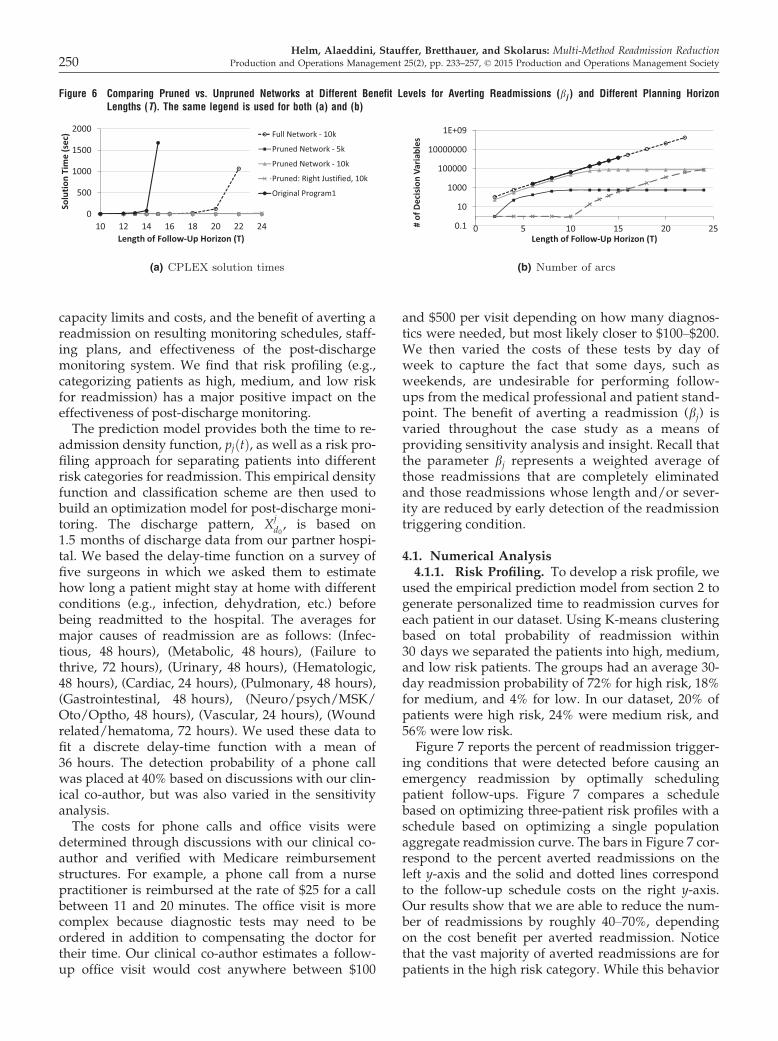
capacity limits and costs, and the benefit of averting areadmission on resulting monitoring schedules, staff-ing plans, and effectiveness of the post-dischargemonitoring system. We find that risk profiling (e.g.,categorizing patients as high, medium, and low riskfor readmission) has a major positive impact on theeffectiveness of post-discharge monitoring.The prediction model provides both the time to re-

admission density function, pjðtÞ, as well as a risk pro-filing approach for separating patients into differentrisk categories for readmission. This empirical densityfunction and classification scheme are then used tobuild an optimization model for post-discharge moni-toring. The discharge pattern, X

jd0, is based on

1.5 months of discharge data from our partner hospi-tal. We based the delay-time function on a survey offive surgeons in which we asked them to estimatehow long a patient might stay at home with differentconditions (e.g., infection, dehydration, etc.) beforebeing readmitted to the hospital. The averages formajor causes of readmission are as follows: (Infec-tious, 48 hours), (Metabolic, 48 hours), (Failure tothrive, 72 hours), (Urinary, 48 hours), (Hematologic,48 hours), (Cardiac, 24 hours), (Pulmonary, 48 hours),(Gastrointestinal, 48 hours), (Neuro/psych/MSK/Oto/Optho, 48 hours), (Vascular, 24 hours), (Woundrelated/hematoma, 72 hours). We used these data tofit a discrete delay-time function with a mean of36 hours. The detection probability of a phone callwas placed at 40% based on discussions with our clin-ical co-author, but was also varied in the sensitivityanalysis.The costs for phone calls and office visits were

determined through discussions with our clinical co-author and verified with Medicare reimbursementstructures. For example, a phone call from a nursepractitioner is reimbursed at the rate of $25 for a callbetween 11 and 20 minutes. The office visit is morecomplex because diagnostic tests may need to beordered in addition to compensating the doctor fortheir time. Our clinical co-author estimates a follow-up office visit would cost anywhere between $100

and $500 per visit depending on how many diagnos-tics were needed, but most likely closer to $100–$200.We then varied the costs of these tests by day ofweek to capture the fact that some days, such asweekends, are undesirable for performing follow-ups from the medical professional and patient stand-point. The benefit of averting a readmission (bj) isvaried throughout the case study as a means ofproviding sensitivity analysis and insight. Recall thatthe parameter bj represents a weighted average ofthose readmissions that are completely eliminatedand those readmissions whose length and/or sever-ity are reduced by early detection of the readmissiontriggering condition.

4.1. Numerical Analysis4.1.1. Risk Profiling. To develop a risk profile, we

used the empirical prediction model from section 2 togenerate personalized time to readmission curves foreach patient in our dataset. Using K-means clusteringbased on total probability of readmission within30 days we separated the patients into high, medium,and low risk patients. The groups had an average 30-day readmission probability of 72% for high risk, 18%for medium, and 4% for low. In our dataset, 20% ofpatients were high risk, 24% were medium risk, and56% were low risk.Figure 7 reports the percent of readmission trigger-

ing conditions that were detected before causing anemergency readmission by optimally schedulingpatient follow-ups. Figure 7 compares a schedulebased on optimizing three-patient risk profiles with aschedule based on optimizing a single populationaggregate readmission curve. The bars in Figure 7 cor-respond to the percent averted readmissions on theleft y-axis and the solid and dotted lines correspondto the follow-up schedule costs on the right y-axis.Our results show that we are able to reduce the num-ber of readmissions by roughly 40–70%, dependingon the cost benefit per averted readmission. Noticethat the vast majority of averted readmissions are forpatients in the high risk category. While this behavior

0

500

1000

1500

2000

10 12 14 16 18 20 22 24

Solu

tion

Tim

e (s

ec)

Length of Follow-Up Horizon (T)

Full Network - 10k

Pruned Network - 5k

Pruned Network - 10k

Pruned: Right Justified, 10k

Original Program1

0.1

10

1000

100000

10000000

1E+09

0 5 10 15 20 25# of

Dec

isio

n Va

riabl

es

Length of Follow-Up Horizon (T)

(a) (b)

Figure 6 Comparing Pruned vs. Unpruned Networks at Different Benefit Levels for Averting Readmissions (bj ) and Different Planning HorizonLengths (T). The same legend is used for both (a) and (b)


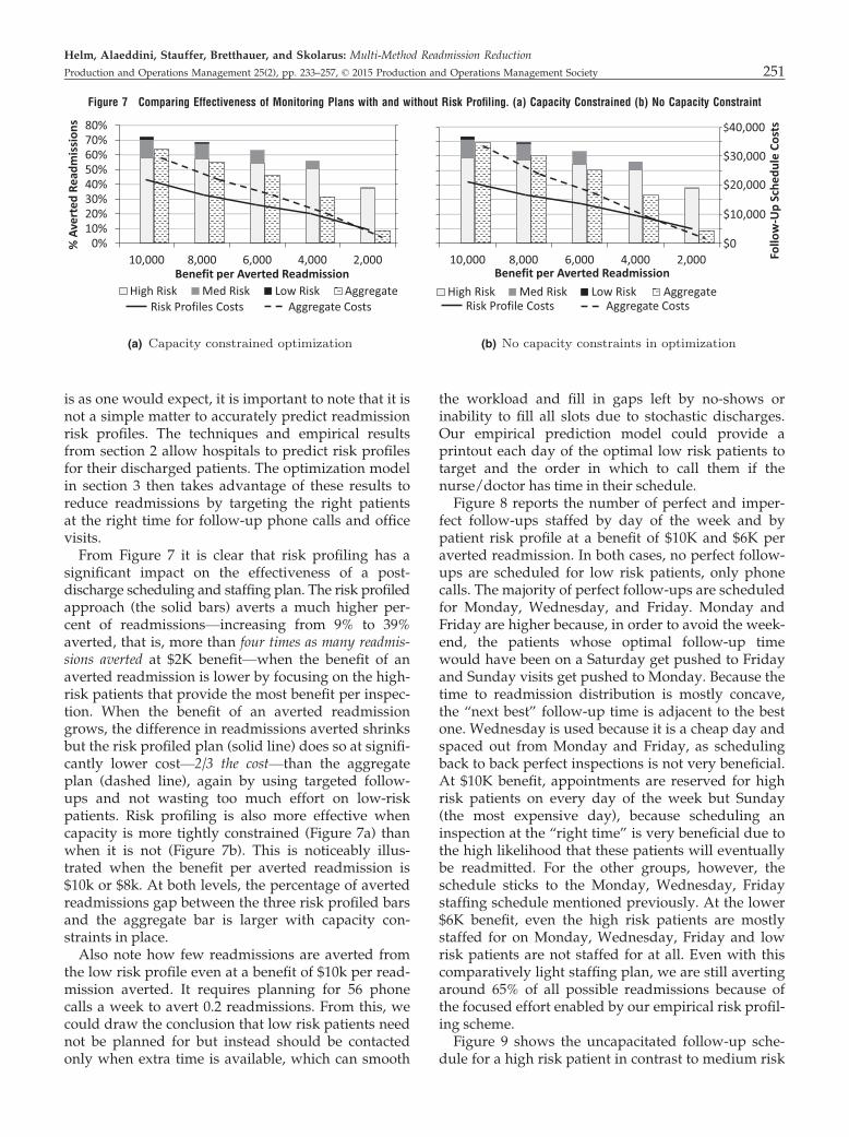
is as one would expect, it is important to note that it isnot a simple matter to accurately predict readmissionrisk profiles. The techniques and empirical resultsfrom section 2 allow hospitals to predict risk profilesfor their discharged patients. The optimization modelin section 3 then takes advantage of these results toreduce readmissions by targeting the right patientsat the right time for follow-up phone calls and officevisits.From Figure 7 it is clear that risk profiling has a

significant impact on the effectiveness of a post-discharge scheduling and staffing plan. The risk profiledapproach (the solid bars) averts a much higher per-cent of readmissions—increasing from 9% to 39%averted, that is, more than four times as many readmis-sions averted at $2K benefit—when the benefit of anaverted readmission is lower by focusing on the high-risk patients that provide the most benefit per inspec-tion. When the benefit of an averted readmissiongrows, the difference in readmissions averted shrinksbut the risk profiled plan (solid line) does so at signifi-cantly lower cost—2/3 the cost—than the aggregateplan (dashed line), again by using targeted follow-ups and not wasting too much effort on low-riskpatients. Risk profiling is also more effective whencapacity is more tightly constrained (Figure 7a) thanwhen it is not (Figure 7b). This is noticeably illus-trated when the benefit per averted readmission is$10k or $8k. At both levels, the percentage of avertedreadmissions gap between the three risk profiled barsand the aggregate bar is larger with capacity con-straints in place.Also note how few readmissions are averted from

the low risk profile even at a benefit of $10k per read-mission averted. It requires planning for 56 phonecalls a week to avert 0.2 readmissions. From this, wecould draw the conclusion that low risk patients neednot be planned for but instead should be contactedonly when extra time is available, which can smooth

the workload and fill in gaps left by no-shows orinability to fill all slots due to stochastic discharges.Our empirical prediction model could provide aprintout each day of the optimal low risk patients totarget and the order in which to call them if thenurse/doctor has time in their schedule.Figure 8 reports the number of perfect and imper-

fect follow-ups staffed by day of the week and bypatient risk profile at a benefit of $10K and $6K peraverted readmission. In both cases, no perfect follow-ups are scheduled for low risk patients, only phonecalls. The majority of perfect follow-ups are scheduledfor Monday, Wednesday, and Friday. Monday andFriday are higher because, in order to avoid the week-end, the patients whose optimal follow-up timewould have been on a Saturday get pushed to Fridayand Sunday visits get pushed to Monday. Because thetime to readmission distribution is mostly concave,the “next best” follow-up time is adjacent to the bestone. Wednesday is used because it is a cheap day andspaced out from Monday and Friday, as schedulingback to back perfect inspections is not very beneficial.At $10K benefit, appointments are reserved for highrisk patients on every day of the week but Sunday(the most expensive day), because scheduling aninspection at the “right time” is very beneficial due tothe high likelihood that these patients will eventuallybe readmitted. For the other groups, however, theschedule sticks to the Monday, Wednesday, Fridaystaffing schedule mentioned previously. At the lower$6K benefit, even the high risk patients are mostlystaffed for on Monday, Wednesday, Friday and lowrisk patients are not staffed for at all. Even with thiscomparatively light staffing plan, we are still avertingaround 65% of all possible readmissions because ofthe focused effort enabled by our empirical risk profil-ing scheme.Figure 9 shows the uncapacitated follow-up sche-

dule for a high risk patient in contrast to medium risk

0%10%20%30%40%50%60%70%80%

10,000 8,000 6,000 4,000 2,000

% A

vert

ed R

eadm

issi

ons

Benefit per Averted ReadmissionHigh Risk Med Risk Low Risk Aggregate

Risk Profiles Costs Aggregate Costs

10,000 8,000 6,000 4,000 2,000Benefit per Averted Readmission

High Risk Med Risk Low Risk AggregateRisk Profile Costs Aggregate Costs

$0

$20,000

$10,000

$30,000

$40,000

Follo

w-U

p Sc

hedu

le C

osts

(a) (b)

Figure 7 Comparing Effectiveness of Monitoring Plans with and without Risk Profiling. (a) Capacity Constrained (b) No Capacity Constraint



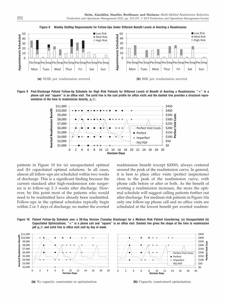
patients in Figure 10 for (a) uncapacitated optimaland (b) capacitated optimal solutions. In all cases,almost all follow-ups are scheduled within two weeksof discharge. This is a significant finding because thecurrent standard after high-readmission rate surger-ies is to follow-up 2–3 weeks after discharge. How-ever, by this point most of the patients who wouldneed to be readmitted have already been readmitted.Follow-ups in the optimal schedules typically beginwithin 2 or 3 days of discharge, no matter the averted

readmission benefit (except $2000), always centeredaround the peak of the readmission curve. In general,it is best to place office visits (perfect inspections)close to the peak of the readmission curve, withphone calls before or after or both. As the benefit ofaverting a readmission increases, the more the opti-mal schedule will suggest calling patients further outafter discharge. For medium risk patients in Figure 10aonly one follow-up phone call and no office visits arescheduled at the lowest benefit per averted readmis-

$2,000$3,000$4,000$5,000$6,000$7,000$8,000$9,000

$10,000$11,000

0 2 4 6 8 10 12 14 16 18 20

Aver

ted

Read

mis

sion

Bene

fit

Horizon Days

$0$50$100$150$200$250$300$350$400$450

0 2 4 6 8 10 12 14 16 18 20

Perf

ectV

isit

Cost

Horizon Days

Perfect Visit CostsPerfectImperfectP(t) PDF

(a) (b)

Figure 10 Patient Follow-Up Schedule over a 30-Day Horizon (Tuesday Discharge) for a Medium Risk Patient Considering: (a) Uncapacitated (b)Capacitated Optimizations. “3” is a phone call and “square” is an office visit. Dashed line gives the shape of the time to readmissionpdf pj ðtÞ and solid line is office visit cost by day of week.

01020304050

Per Imp Per Imp Per Imp Per Imp Per Imp Per Imp Per Imp

Mon Tues Wed Thur Fri Sat SunAppo

intm

ents

Sche

dule

d Low RiskMed RiskHigh Risk

010203040

Per Imp Per Imp Per Imp Per Imp Per Imp Per Imp Per Imp


intm

ents

Sche

dule

d Low RiskMed RiskHigh Risk

50

(a) (b)

Figure 8 Weekly Staffing Requirements for Follow-Ups Under Different Benefit Levels of Averting a Readmission

Figure 9 Post-Discharge Patient Follow-Up Schedule for High Risk Patients for Different Levels of Benefit of Averting a Readmission. “3” is aphone call and “square” is an office visit. The solid line is the cost profile for office visits and the dashed line provides a structural repre-sentation of the time to readmission density, pj ðtÞ.


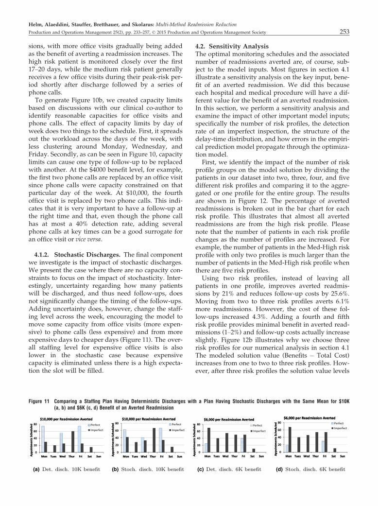
sions, with more office visits gradually being addedas the benefit of averting a readmission increases. Thehigh risk patient is monitored closely over the first17–20 days, while the medium risk patient generallyreceives a few office visits during their peak-risk per-iod shortly after discharge followed by a series ofphone calls.To generate Figure 10b, we created capacity limits

based on discussions with our clinical co-author toidentify reasonable capacities for office visits andphone calls. The effect of capacity limits by day ofweek does two things to the schedule. First, it spreadsout the workload across the days of the week, withless clustering around Monday, Wednesday, andFriday. Secondly, as can be seen in Figure 10, capacitylimits can cause one type of follow-up to be replacedwith another. At the $4000 benefit level, for example,the first two phone calls are replaced by an office visitsince phone calls were capacity constrained on thatparticular day of the week. At $10,000, the fourthoffice visit is replaced by two phone calls. This indi-cates that it is very important to have a follow-up atthe right time and that, even though the phone callhas at most a 40% detection rate, adding severalphone calls at key times can be a good surrogate foran office visit or vice versa.

4.1.2. Stochastic Discharges. The final componentwe investigate is the impact of stochastic discharges.We present the case where there are no capacity con-straints to focus on the impact of stochasticity. Inter-estingly, uncertainty regarding how many patientswill be discharged, and thus need follow-ups, doesnot significantly change the timing of the follow-ups.Adding uncertainty does, however, change the staff-ing level across the week, encouraging the model tomove some capacity from office visits (more expen-sive) to phone calls (less expensive) and from moreexpensive days to cheaper days (Figure 11). The over-all staffing level for expensive office visits is alsolower in the stochastic case because expensivecapacity is eliminated unless there is a high expecta-tion the slot will be filled.

4.2. Sensitivity AnalysisThe optimal monitoring schedules and the associatednumber of readmissions averted are, of course, sub-ject to the model inputs. Most figures in section 4.1illustrate a sensitivity analysis on the key input, bene-fit of an averted readmission. We did this becauseeach hospital and medical procedure will have a dif-ferent value for the benefit of an averted readmission.In this section, we perform a sensitivity analysis andexamine the impact of other important model inputs;specifically the number of risk profiles, the detectionrate of an imperfect inspection, the structure of thedelay-time distribution, and how errors in the empiri-cal prediction model propagate through the optimiza-tion model.First, we identify the impact of the number of risk

profile groups on the model solution by dividing thepatients in our dataset into two, three, four, and fivedifferent risk profiles and comparing it to the aggre-gated or one profile for the entire group. The resultsare shown in Figure 12. The percentage of avertedreadmissions is broken out in the bar chart for eachrisk profile. This illustrates that almost all avertedreadmissions are from the high risk profile. Pleasenote that the number of patients in each risk profilechanges as the number of profiles are increased. Forexample, the number of patients in the Med-High riskprofile with only two profiles is much larger than thenumber of patients in the Med-High risk profile whenthere are five risk profiles.Using two risk profiles, instead of leaving all

patients in one profile, improves averted readmis-sions by 21% and reduces follow-up costs by 25.6%.Moving from two to three risk profiles averts 6.1%more readmissions. However, the cost of these fol-low-ups increased 4.3%. Adding a fourth and fifthrisk profile provides minimal benefit in averted read-missions (1–2%) and follow-up costs actually increaseslightly. Figure 12b illustrates why we choose threerisk profiles for our numerical analysis in section 4.1The modeled solution value (Benefits � Total Cost)increases from one to two to three risk profiles. How-ever, after three risk profiles the solution value levels

0

20

40

60

80


intm

ents

Sche

dule

d

$10,000 per Readmission AvertedPerfect

Imperfect

0

20

40

60

80


intm

ents

Sche

dule

d


Imperfect

0

20

40

60

80


intm

ents

Sche

dule

d


Imperfect

0

20

40

60

80


intm

ents

Sche

dule

d

$6,000 per Readmission AvertedPerfectImperfect

0

20

40

60

80


intm

ents

Sche

dule

d


Imperfect

0

20

40

60

80


intm

ents

Sche

dule

d


Imperfect

0

20

40

60

80


intm

ents

Sche

dule

d


Imperfect

0

20

40

60

80


intm

ents

Sche

dule

d

$6,000 per Readmission AvertedPerfectImperfect

(a) (b) St (c) (d)

Figure 11 Comparing a Staffing Plan Having Deterministic Discharges with a Plan Having Stochastic Discharges with the Same Mean for $10K(a, b) and $6K (c, d) Benefit of an Averted Readmission



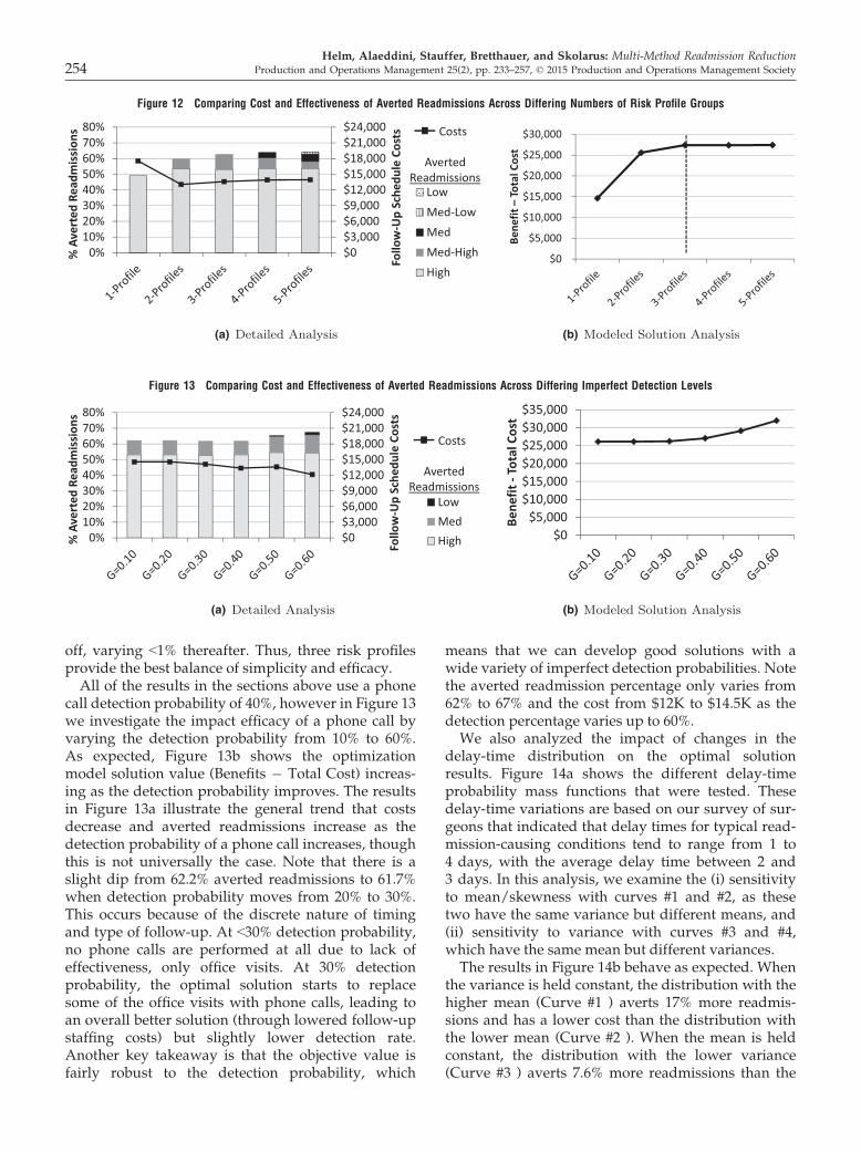
off, varying <1% thereafter. Thus, three risk profilesprovide the best balance of simplicity and efficacy.All of the results in the sections above use a phone

call detection probability of 40%, however in Figure 13we investigate the impact efficacy of a phone call byvarying the detection probability from 10% to 60%.As expected, Figure 13b shows the optimizationmodel solution value (Benefits � Total Cost) increas-ing as the detection probability improves. The resultsin Figure 13a illustrate the general trend that costsdecrease and averted readmissions increase as thedetection probability of a phone call increases, thoughthis is not universally the case. Note that there is aslight dip from 62.2% averted readmissions to 61.7%when detection probability moves from 20% to 30%.This occurs because of the discrete nature of timingand type of follow-up. At <30% detection probability,no phone calls are performed at all due to lack ofeffectiveness, only office visits. At 30% detectionprobability, the optimal solution starts to replacesome of the office visits with phone calls, leading toan overall better solution (through lowered follow-upstaffing costs) but slightly lower detection rate.Another key takeaway is that the objective value isfairly robust to the detection probability, which

means that we can develop good solutions with awide variety of imperfect detection probabilities. Notethe averted readmission percentage only varies from62% to 67% and the cost from $12K to $14.5K as thedetection percentage varies up to 60%.We also analyzed the impact of changes in the

delay-time distribution on the optimal solutionresults. Figure 14a shows the different delay-timeprobability mass functions that were tested. Thesedelay-time variations are based on our survey of sur-geons that indicated that delay times for typical read-mission-causing conditions tend to range from 1 to4 days, with the average delay time between 2 and3 days. In this analysis, we examine the (i) sensitivityto mean/skewness with curves #1 and #2, as thesetwo have the same variance but different means, and(ii) sensitivity to variance with curves #3 and #4,which have the same mean but different variances.The results in Figure 14b behave as expected. When

the variance is held constant, the distribution with thehigher mean (Curve #1 ) averts 17% more readmis-sions and has a lower cost than the distribution withthe lower mean (Curve #2 ). When the mean is heldconstant, the distribution with the lower variance(Curve #3 ) averts 7.6% more readmissions than the

$0$3,000$6,000$9,000$12,000$15,000$18,000$21,000$24,000

0%10%20%30%40%50%60%70%80%

Follo

w-U

pSc

hedu

leCo

sts

%Av

erte

dRe

adm

issi

ons

LowMed-LowMedMed-HighHigh

Costs

AvertedReadmissions

$0

$5,000

$10,000

$15,000

$20,000

$25,000

$30,000

Bene

fit–

Tota

lCos

t

(a) (b)

Figure 12 Comparing Cost and Effectiveness of Averted Readmissions Across Differing Numbers of Risk Profile Groups

$0$3,000$6,000$9,000$12,000$15,000$18,000$21,000$24,000

0%10%20%30%40%50%60%70%80%

Follo

w-U

p Sc

hedu

le C

osts

% A

vert

ed R

eadm

issi

ons

LowMedHigh

Costs

Averted Readmissions

$0$5,000

$10,000$15,000$20,000$25,000$30,000$35,000

Bene

fit -

Tota

l Cos

t

(a) (b)

Figure 13 Comparing Cost and Effectiveness of Averted Readmissions Across Differing Imperfect Detection Levels


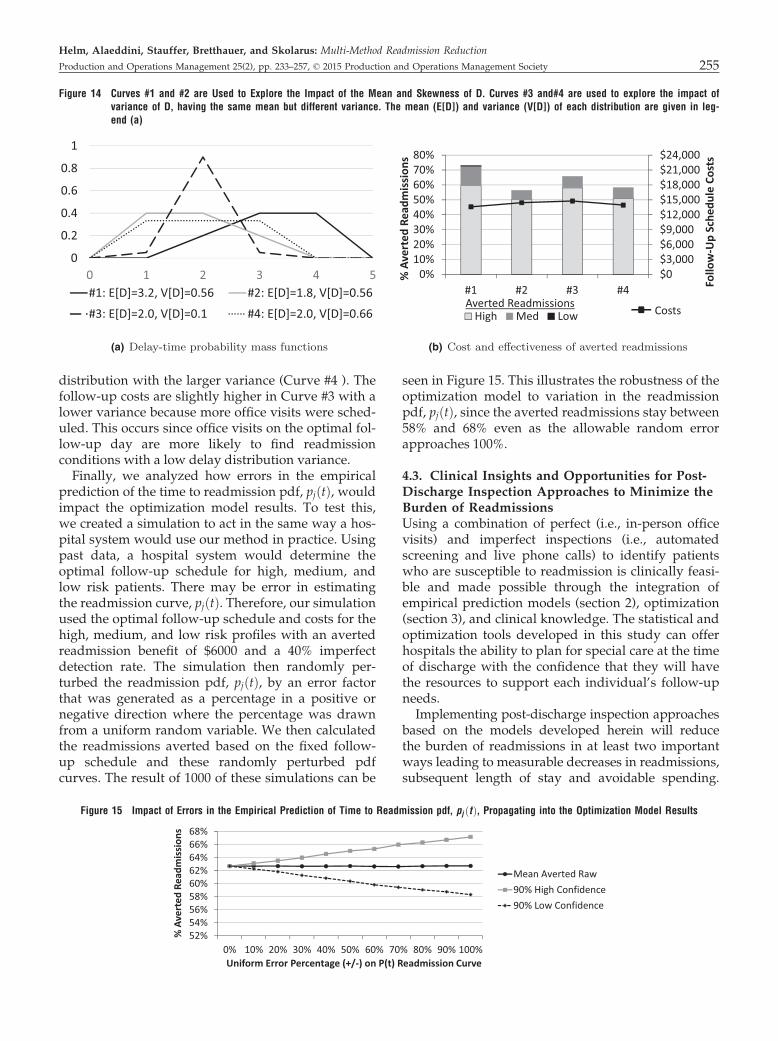
distribution with the larger variance (Curve #4 ). Thefollow-up costs are slightly higher in Curve #3 with alower variance because more office visits were sched-uled. This occurs since office visits on the optimal fol-low-up day are more likely to find readmissionconditions with a low delay distribution variance.Finally, we analyzed how errors in the empirical

prediction of the time to readmission pdf, pjðtÞ, wouldimpact the optimization model results. To test this,we created a simulation to act in the same way a hos-pital system would use our method in practice. Usingpast data, a hospital system would determine theoptimal follow-up schedule for high, medium, andlow risk patients. There may be error in estimatingthe readmission curve, pjðtÞ. Therefore, our simulationused the optimal follow-up schedule and costs for thehigh, medium, and low risk profiles with an avertedreadmission benefit of $6000 and a 40% imperfectdetection rate. The simulation then randomly per-turbed the readmission pdf, pjðtÞ, by an error factorthat was generated as a percentage in a positive ornegative direction where the percentage was drawnfrom a uniform random variable. We then calculatedthe readmissions averted based on the fixed follow-up schedule and these randomly perturbed pdfcurves. The result of 1000 of these simulations can be

seen in Figure 15. This illustrates the robustness of theoptimization model to variation in the readmissionpdf, pjðtÞ, since the averted readmissions stay between58% and 68% even as the allowable random errorapproaches 100%.

4.3. Clinical Insights and Opportunities for Post-Discharge Inspection Approaches to Minimize theBurden of ReadmissionsUsing a combination of perfect (i.e., in-person officevisits) and imperfect inspections (i.e., automatedscreening and live phone calls) to identify patientswho are susceptible to readmission is clinically feasi-ble and made possible through the integration ofempirical prediction models (section 2), optimization(section 3), and clinical knowledge. The statistical andoptimization tools developed in this study can offerhospitals the ability to plan for special care at the timeof discharge with the confidence that they will havethe resources to support each individual’s follow-upneeds.Implementing post-discharge inspection approaches

based on the models developed herein will reducethe burden of readmissions in at least two importantways leading to measurable decreases in readmissions,subsequent length of stay and avoidable spending.

0

0.2

0.4

0.6

0.8

1

0 1 2 3 4 5#1: E[D]=3.2, V[D]=0.56 #2: E[D]=1.8, V[D]=0.56

#3: E[D]=2.0, V[D]=0.1 #4: E[D]=2.0, V[D]=0.66

$0$3,000$6,000$9,000$12,000$15,000$18,000$21,000$24,000

0%10%20%30%40%50%60%70%80%

#1 #2 #3 #4 Follo

w-U

pSc

hedu

leCo

sts

%Av

erte

dRe

adm

issi

ons

High Med Low CostsAverted Readmissions

(a) (b)

Figure 14 Curves #1 and #2 are Used to Explore the Impact of the Mean and Skewness of D. Curves #3 and#4 are used to explore the impact ofvariance of D, having the same mean but different variance. The mean (E[D]) and variance (V[D]) of each distribution are given in leg-end (a)

52%54%56%58%60%62%64%66%68%

0% 10% 20% 30% 40% 50% 60% 70% 80% 90% 100%

% A

vert

ed R

eadm

issi

ons

Uniform Error Percentage (+/-) on P(t) Readmission Curve

Mean Averted Raw90% High Confidence90% Low Confidence

Figure 15 Impact of Errors in the Empirical Prediction of Time to Readmission pdf, pj ðtÞ, Propagating into the Optimization Model Results



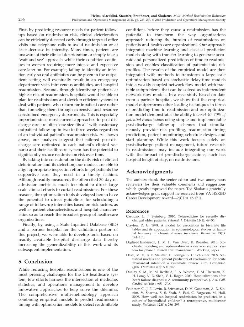
First, by predicting resource needs for patient follow-ups based on readmission risk, clinical deteriorationcan be efficiently detected early through targeted officevisits and telephone calls to avoid readmission or atleast decrease its intensity. Many times, patients areunaware of their clinical deterioration or simply take a‘wait-and-see’ approach while their condition contin-ues to worsen requiring more intense and expensivecare later on. For example, failing to identify an infec-tion early so oral antibiotics can be given in the outpa-tient setting will eventually result in an emergencydepartment visit, intravenous antibiotics, and hospitalreadmission. Second, through identifying patients athighest risk of readmission, hospitals would be able toplan for readmissions and develop efficient systems todeal with patients who return for inpatient care ratherthan funneling them through expensive and resourceconstrained emergency departments. This is especiallyimportant since most current approaches to post-dis-charge care are often ‘one-size fits all’ with customaryoutpatient follow-up in two to three weeks regardlessof an individual patient’s readmission risk. As shownabove, our analyses suggest that tailored post-dis-charge care optimized to each patient’s clinical sce-nario and their health-care system has the potential tosignificantly reduce readmission risk over time.By taking into consideration the daily risk of clinical

deterioration and its detection, our models are able toalign appropriate inspection efforts to get patients thesupportive care they need in a timely fashion.Although readily measured, the often cited 30-day re-admission metric is much too blunt to direct largescale clinical efforts to curtail readmissions. For thesereasons, the optimization tools developed herein havethe potential to direct guidelines for scheduling arange of follow-up intensities based on risk factors, aswell as patient characteristics, and hospital character-istics so as to reach the broadest group of health-careorganizations.Finally, by using a State Inpatient Database (SID)

and a partner hospital for the validation portion ofthis project, we were able to develop tools based onreadily available hospital discharge data therebyincreasing the generalizability of this work and itssubsequent implementation.

5. Conclusion

While reducing hospital readmissions is one of themost pressing challenges for the US healthcare sys-tem, few efforts harness the intersection of medicine,statistics, and operations management to developinnovative approaches to help solve the dilemma.The comprehensive multi-methodology approachcombining empirical models to predict readmissiontiming with optimization models to detect readmittable

conditions before they cause a readmission has thepotential to transform the way organizationsapproach reducing the burden of readmissions onpatients and health-care organizations. Our approachintegrates machine learning and classical predictionmodels along with transfer learning to generate accu-rate and personalized predictions of time to readmis-sion and enables classification of patients into riskprofiles. The results of the empirical model are thenintegrated with methods to transform a large-scaleoptimization based on stochastic delay-time modelsinto a weakly coupled network flow model with trac-table subproblems that can be solved as independentnetwork flow models. In a case study based on datafrom a partner hospital, we show that the empiricalmodel outperforms other leading techniques in termsof predicting time to readmission and our optimiza-tion model demonstrates the ability to avert 40–70% ofpotential readmissions using simple and implementablepost-discharge follow-up schemes that simulta-neously provide risk profiling, readmission timingprediction, patient monitoring schedule design, andstaff planning. While this work focuses solely onpost-discharge patient management, future researchin readmissions may include integrating our workwith the impact of pre-discharge actions, such hashospital length of stay, on readmissions.

Acknowledgments

The authors thank the senior editor and two anonymousreviewers for their valuable comments and suggestionswhich greatly improved the paper. Ted Skolarus gratefullyacknowledges grant support he received from VA HSR&DCareer Development Award—2(CDA 12-171).

ReferencesCardozo, L., J. Steinberg. 2010. Telemedicine for recently dis-

charged older patients. Telemed. J. E-Health 16(1): 49–55.

Clayton, D. G. 1978. A model for association in bivariate lifetables and its application in epidemiological studies of famil-ial tendency in chronic disease incidence. Biometrika 65(1):141–151.

Deglise-Hawkinson, J., M. P. Van Oyen, B. Roessler. 2013. Sto-chastic modeling and optimization in a decision support sys-tem for phase 1 clinical trial management. Working paper.

Desai, M. M, B. D. Stauffer, H. Feringa, G. C. Schreiner. 2009. Sta-tistical models and patient predictors of readmission for acutemyocardial infarction a systematic review. Circ. Cardiovasc.Qual. Outcomes 2(5): 500–507.

Dunlay, S. M., M. M. Redfield, S. A. Weston, T. M. Therneau, K.H. Long, N. D. Shah, V. L. Roger. 2009. Hospitalizations afterheart failure diagnosis: A community perspective. J. Am. Coll.Cardiol. 54(18): 1695–1702.

Feudtner, C., J. E. Levin, R. Srivastava, D. M. Goodman, A. D. Slo-nim, V. Sharma, S. S. Shah, S. Pati, C. Fargason, M. Hall.2009. How well can hospital readmission be predicted in acohort of hospitalized children? a retrospective, multicenterstudy. Pediatrics 123(1): 286–293.


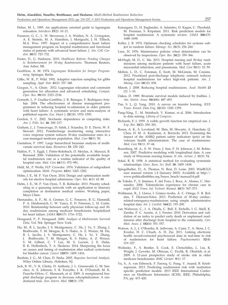
Fisher, M. L. 1985. An applications oriented guide to lagrangianrelaxation. Interfaces 15(2): 10–21.

Fonarow, G. C., L. W. Stevenson, J. A. Walden, N. A. Livingston,A. E. Steimle, M. A. Hamilton, J. Moriguchi, J. H. Tillisch,M.A. Woo. 1997. Impact of a comprehensive heart failuremanagement program on hospital readmission and functionalstatus of patients with advanced heart failure. J. Am. Coll. Car-diol. 30(3): 725–732.

Foster, D., G. Harkness. 2010. Healthcare Reform: Pending Changesto Reimbursement for 30-day Readmissions. Thomson Reuters,Ann Arbor, MI.

Geoffrion, A. M. 1974. Lagrangean Relaxation for Integer Program-ming. Springer, Berlin.

Gilks, W. R., P. Wild. 1992. Adaptive rejection sampling for gibbssampling. Appl. Stat. 41(2): 337–348.

Gocgun, Y., A. Ghate. 2012. Lagrangian relaxation and constraintgeneration for allocation and advanced scheduling. Comput.Oper. Res. 39(10): 2323–2336.

Gonseth, J., P. Guallar-Castill�on, J. R. Banegas, F. Rodr�ıguez-Arta-lejo. 2004. The effectiveness of disease management pro-grammes in reducing hospital re-admission in older patientswith heart failure: A systematic review and meta-analysis ofpublished reports. Eur. Heart J. 25(18): 1570–1595.

Gordon, S. C. 2002. Stochastic dependence in competing risks.Am. J. Polit. Sci. 46: 200–217.

Graham, J., J. Tomcavage, D. Salek, J. Sciandra, D. E. Davis, W. F.Stewart. 2012. Postdischarge monitoring using interactivevoice response system reduces 30-day readmission rates in acase-managed medicare population. Med. Care 50(1): 50.

Gustafson, P. 1997. Large hierarchical bayesian analysis of multi-variate survival data. Biometrics 53: 230–242.

Halfon, P., Y. Eggli, I. Pretre-Rohrbach, D. Meylan, A. Marazzi, B.Burnand. 2006. Validation of the potentially avoidable hospi-tal readmission rate as a routine indicator of the quality ofhospital care. Med. Care 44(11): 972–981.

Held, M., P. Wolfe, H.P. Crowder. 1974. Validation of subgradientoptimization. Math. Program. 62(6): 1265–1282.

Helm, J. E., M. P. Van Oyen. 2014. Design and optimization meth-ods for elective hospital admissions. Oper. Res. 6(1): 62–88

Helm, J. E., M. P. Van Oyen, T. R. Rohleder. 2013. Priority sched-uling in a queueing network with an application to itinerarycompletion at destination medical centers. Working paper,Mayo Clinic.

Hernandez, A. F., M. A. Greiner, G. C. Fonarow, B. G. Hammill,P. A. Heidenreich, C. W. Yancy, E. D. Peterson, L. H. Curtis.2010. Relationship between early physician follow-up and 30-day readmission among medicare beneficiaries hospitalizedfor heart failure. JAMA 303(17): 1716–1722.

Hougaard, P., P. Hougaard. 2000. Analysis of Multivariate SurvivalData, Vol. 564. Springer New York.

Hu, M., B. L. Jacobs, J. S. Montgomery, C. He, J. Ye, Y. Zhang, J.Brathwaite, T. M. Morgan, K. S. Hafez, A. Z. Weizer, M. Hu,B. L. Jacobs, J. S. Montgomery, C. He, J. Ye, Y. Zhang,J. Brathwaite, T. M. Morgan, K. S. Hafez, A. Z. Weizer,S. M. Gilbert, C. T Lee, M. S. Lavieri, J. E. Helm,B. K. Hollenbeck, T. A. Skolarus. 2014. Sharpening the focuson causes and timing of readmission after radical cystectomyfor bladder cancer. Cancer 120(9): 1409–1416.

Ibrahim, J. G., M. Chen, D. Sinha. 2005. Bayesian Survival Analysis.Wiley Online Library, Hoboken, NJ.

Jack, B. W., V. K. Chetty, D. Anthony, J. L. Greenwald, G. M. San-chez, A. E. Johnson, S. R. Forsythe, J. K. O’Donnell, M. K.Paasche-Orlow, C. Manasseh, et al. 2009. A reengineered hos-pital discharge program to decrease rehospitalization: A ran-domized trial. Ann. Intern. Med. 150(3): 178.

Kansagara, D., H. Englander, A. Salanitro, D. Kagen, C. Theobald,M. Freeman, S. Kripalani. 2011. Risk prediction models forhospital readmission: A systematic review. JAMA 306(15):1688–1698.

Keller, J. B. 1974. Optimum checking schedules for systems sub-ject to random failure. Manage. Sci. 21(3): 256–260.

Luss, H. 1976. Maintenance policies when deterioration can beobserved by inspections. Oper. Res. 24(2): 359–366.

McHugh, M. D., C. Ma. 2013. Hospital nursing and 30-day read-missions among medicare patients with heart failure, acutemyocardial infarction, and pneumonia. Med. Care 51(1): 52–59.

Melton, L. D., C. Foreman, E. Scott, M. McGinnis, M. Cousins.2012. Prioritized post-discharge telephonic outreach reduceshospital readmissions for select high-risk patients. Am. J.Manag. Care 18(12): 838.

Minott, J. 2008. Reducing hospital readmissions. Acad. Health 23(2): 1–10.

Oakes, D. 1989. Bivariate survival models induced by frailties. J.Am. Statist. Assoc. 84(406): 487–493.

Pan, S. J., Q. Yang. 2010. A survey on transfer learning. IEEETrans. Knowl. Data Eng. 22(10): 1345–1359.

Pang-Ning, T., M. Steinbach, V. Kumar, et al. 2006. Introductionto data mining. Library of Congress.

Richards, F. J. 1959. A exible growth function for empirical use. J.Exp. Bot. 10(2): 290–301.

Rosen, A. K., S. Loveland, M. Shin, M. Shwartz, A. Hanchate, Q.Chen, H. M. A. Kaafarani, A. Borzecki. 2013. Examining theimpact of the AHRQ patient safety indicators (psis) on theveterans health administration: The case of readmissions.Med. Care 51(1): 37–44.

Rosenberg, M. A., E. W. Frees, J. Sun, P. H. Johnson, J. M. Robin-son. 2007. Predictive modeling with longitudinal data: A casestudy of Wisconsin nursing homes. N Am. Actuar. J. 11(3): 54.

Sokal, R. R. 1958. A statistical method for evaluating systematicrelationships. Univ. Kans. Sci. Bull. 38: 1409–1438.

Spiegelhalter, D., A. Thomas, N. Best, D. Lunn. 2003. WinBUGSuser manual version 1.4 (January 2003). Available at http://www.politicalbubbles.org/bayes_beach/manual14.pdf

de Toledo, P., S. Jim�enez, F. del Pozo, J. Roca, A. Alonso, C. Her-nandez. 2006. Telemedicine experience for chronic care incopd. IEEE Trans. Inf. Technol. Biomed. 10(3): 567–573.

Wallmann, R., J. Llorca, I. G�omez-Acebo, �A. C. Ortega, F. R. Rol-dan, T. Dierssen-Sotos. 2013. Prediction of 30-day cardiac-related-emergency-readmissions using simple administrativehospital data. Int. J. Cardiol. 164(2): 193–200.

van Walraven, C., I. A. Dhalla, C. Bell, E. Etchells, I. G. Stiell, K.Zarnke, P. C. Austin, A. J. Forster. 2010. Derivation and vali-dation of an index to predict early death or unplanned read-mission after discharge from hospital to the community. Can.Med. Assoc. J. 182(6): 551–557.

Watson, A. J., J. O’Rourke, K. Jethwani, A. Cami, T. A. Stern, J. C.Kvedar, H. C. Chueh, A. H. Zai. 2011. Linking electronichealth record-extracted psychosocial data in real-time to riskof readmission for heart failure. Psychosomatics 52(4):319–327.

Wolinsky, F., S. Bentler, E. Cook, E. Chrischilles, L. Liu, K.Wright, J. Geweke, M. Obrizan, C. Pavlik, R. Ohsfeldt, et al.2009. A 12-year prospective study of stroke risk in oldermedicare beneficiaries. BMC Geriatr. 9(1): 17.

Yu, S., A. van Esbroeck, F. Farooq, G. Fung, V. Anand, B. Krish-napuram. 2013. Predicting readmission risk with institutionspecific prediction models. 2013 IEEE International Confer-ence on Healthcare Informatics (ICHI), IEEE, Philadelphia,PA, pp. 415–420.



http://www.politicalbubbles.org/bayes_beach/manual14.pdf

http://www.politicalbubbles.org/bayes_beach/manual14.pdf

Reducing Hospital Readmissions by Integrating Empirical …helmjweb/publications/A5 (POM) Re… ·...

Documents

Transcript of Reducing Hospital Readmissions by Integrating Empirical …helmjweb/publications/A5 (POM) Re… ·...