Reduced-Order Framework for Exponential

Stabilization of Periodic Orbits on Parameterized

Hybrid Zero Dynamics Manifolds: Application to

Bipedal Locomotion

Kaveh Akbari Hameda,∗, Jessy W. Grizzleb

aDepartment of Mechanical Engineering, San Diego State University, San Diego, CA

92182-1323 USAbDepartment of Electrical Engineering and Computer Science, University of Michigan,

Ann Arbor, MI 48109-2122, USA

Abstract

This paper shows how controlled-invariant manifolds in hybrid dynamicalsystems can be used to reduce the offline computational burden associatedwith locally exponentially stabilizing periodic orbits. We recently introduceda method to systematically select stabilizing feedback controllers for hybridperiodic orbits from a family of parameterized control laws by solving offlineoptimization problems. These problems search for controller parameters aswell as a set of Lyapunov matrices for the full-order hybrid systems. Whenthe method is applied to mechanical systems with high degrees of freedom(DOF), the number of entries in the Lyapunov matrices may render thenumerical optimization problems prohibitively slow. To address this chal-lenge, the paper considers a family of attractive and parameterized hybridzero dynamics (HZD) manifolds in the state space. It then investigates theproperties of the associated Poincare map to translate the full-order optimiza-tion framework to a reduced-order one on the parameterized HZD manifoldswith lower-dimensional Lyapunov matrices. In addition, the paper providesa systematic approach to numerically compute the Jacobian linearization

∗Corresponding AuthorEmail addresses: kakbarihamed@mail.sdsu.edu (Kaveh Akbari Hamed),

grizzle@umich.edu (Jessy W. Grizzle)URL: http://www-rohan.sdsu.edu/~kavehah/ (Kaveh Akbari Hamed),

http://web.eecs.umich.edu/~grizzle/ (Jessy W. Grizzle)

Preprint submitted to Nonlinear Analysis: Hybrid Systems February 3, 2016

of the parameterized Poincare map on the HZD manifolds. The power ofthe proposed framework is demonstrated by designing a set of stabilizinginput-output linearizing controllers for walking gaits of an underactuated 3Dbipedal robot with 13 DOFs and 6 actuators. It is shown that the number ofdecision variables in the reduced-order optimization problem can be reducedby 70% compared to the full-order one.

Keywords: Hybrid Periodic Orbits, Hybrid Zero Dynamics Manifolds,Reduced-Order Exponential Stabilization Problem, Poincare Map,Underactuated Bipedal Robots

1. Introduction

This paper presents a systematic framework to reduce the computationalburden in the design of feedback controllers that render periodic orbits of hy-brid dynamical systems locally exponentially stable. By investigating prop-erties of the Poincare map, the paper breaks down the exponential stabi-lization problem of hybrid periodic orbits for full-order models into a lower-dimensional one defined for a family of parameterized zero dynamics models.The framework can ameliorate specific challenges in the design of stabilizingcontrollers for bipedal robots arising from high dimensionality and underactu-ation. Specifically, the theoretical innovations are applied to design nonlinearstabilizing controllers for walking gaits of an underactuated 3D bipedal robotwith 13 degrees of freedom (DOFs) and 6 actuators. It is shown that thenumber of decision variables for the lower-dimensional problem is reduced by70% compared to the one for the full-order model.

Models of bipedal walking robots are hybrid with continuous-time phasesto represent the right and left stance phases and discrete-time phases torepresent the contact of the swing leg end with the walking surface [1, 2, 3,4, 5, 6, 7, 8, 9, 10, 11, 12, 13, 14, 15, 16, 17]. Our motivation is to designstabilizing feedback controllers for 3D bipedal robots with high degrees offreedom and underactuation, but the results we present apply to a broaderrange of hybrid dynamical systems [18, 19, 20, 21].

The most basic tool for analyzing the stability of hybrid periodic orbits isthe Poincare return map that describes the evolution of the hybrid model ona hypersurface transversal to the orbits, referred to as the Poincare section [2,18, 22, 23]. An important drawback, however, is that in almost all practical

2

cases, there is no closed-form expression for the Poincare map and it mustbe estimated numerically.

Previous work on bipedal walking has made use of a multi-level feed-back control architecture in which parameters of a continuous-time controllerwere updated in an event-based manner to achieve stable bipedal walking[24, 25, 10, 26, 27, 28, 29, 30, 31, 32, 17, 33, 34]. One drawback of achiev-ing stability via event-based controllers is the potentially large delay betweenthe occurrence of a disturbance and the event-based control effort in the nextsteps. We have recently presented a systematic method to design continuous-time controllers that provide robust stability of a given periodic orbit withoutrelying on event-based controllers [35, 36, 37]. This approach was numericallyand experimentally illustrated to design nonlinear stabilizing controllers forstable walking of an underactuated 3D bipedal robot with point feet and 13DOFs [35, 36, 38]. The video of our experiments is available online [39]. Ref-erence [37] also extended the algorithm to design robust optimal controllersfor hybrid models of bipedal running. Our approach is mainly based on op-timization techniques and matrix inequalities in the full-order state space.Roughly speaking by employing a family of nonlinear controllers parameter-ized by ξ, the evolution of the hybrid system on a Poincare section S can bedescribed by a parameterized Poincare map given by

x[k + 1] = P (x[k], ξ) , k = 0, 1, · · · (1)

whose fixed point x⋆ is assumed to be invariant under the choice of the con-troller parameters ξ. When following the Poincare analysis, the exponentialstabilization problem of the corresponding periodic orbit consists of findingξ such that the following matrix inequality

I (A(ξ),W, γ) :=

[W A(ξ)W⋆ (1− γ)W

]

> 0, (2)

is satisfied, in which A(ξ) ∈ R(n−1)×(n−1) represents the Jacobian linearization

of the Poincare map with respect to x, evaluated at the fixed point x⋆, n isthe order of the hybrid system, W = W⊤ > 0 is a Lyapunov matrix, andγ > 0 denotes a scalar to tune the convergence rate. To look for a set ofcontroller parameters ξ, we then set up an optimization problem as follows[35, 36, 37, 40]

min(ξ,W,γ)

J (ξ, γ) (3)

s.t. I (A(ξ),W, γ) > 0 (4)

3

for some smooth cost function J (., .). We see that the Lyapunov matrix

W contains n(n−1)2

scalar entries. The optimization problem (3) and (4)

requires p + n(n−1)2

+ 1 decision variables, where p represents the dimensionof the controller parameters ξ. When n is significantly large, the numberof the resulting Lyapunov variables becomes dominant and the optimizationproblem may be computationally prohibitive. In order to reduce the numberof decision variables in the optimization framework, we are interested inapplying a change of coordinates in the state space as follows

x :=

[zη

]

:= Ψ (x, ξ) (5)

to translate the optimization problem (3) and (4) into an equivalent one interms of a reduced-order Jacobian and lower-dimensional Lyapunov matricesin the z-coordinates. This important numerical benefit of the coordinatetransform (5) also introduces an analytical challenge because the image of thePoincare section itself may now depend on the parameters, viz Sξ := T (S, ξ),whereas previously the “state space” of the Poincare map was independentof the controller parameters.

The contribution of this paper is to present a systematic framework basedon the concept of hybrid invariant manifolds to reduce the number of deci-sion variables in (3) and (4). The framework assumes a family of parameter-ized output functions to be regulated for the continuous-time portion of thehybrid system using input-output (I-O) linearizing controllers [41]. It alsoassumes a family of parameterized event-based controllers. We remark thatthese event-based laws are not utilized to stabilize orbits. They are insteademployed to make the corresponding parameterized zero dynamics manifoldshybrid invariant under the reset map of the hybrid system. The paper theninvestigates the structure of the parameterized Poincare map. It presentsa systematic numerical approach to compute the Jacobian linearization ofthe Poincare map and then develops a reduced-order stability analysis ona parameterized family of Poincare sections. To illustrate the power of theframework, it is finally applied to exponentially stabilize walking gaits of anunderactuated 3D bipedal robot with 13 DOFs. It is shown that the numberof decision variables in the reduced-order framework can be decreased by70% compared to the optimization problem employed in [35].

For dynamical systems with hybrid invariant manifolds, [42] presenteda local coordinate transform under which the Jacobian linearization of the

4

Poincare map has a block upper triangular structure. It also provided con-ditions under which the exponential stabilization problem of periodic orbitsfor the full-order models can be translated to a reduced-order model basedon restricted Poincare maps on the hybrid invariant manifolds. As alludedto earlier, when the controller parameters intervene in the Poincare sectionsand hybrid invariant manifolds, the analysis of the restricted Poincare mapsis more subtle. In particular, reference [42] did not investigate the stabi-lization problem for a family of parameterized manifolds. In addition, it didnot consider the effect of output parameters as well as event-based updatelaws on the Jacobian linearization of the Poincare map. The current paperfirst addresses these issues and subsequently presents a systematic numericalapproach to compute parameterized restricted Poincare maps for a reduced-order framework.

The paper is organized as follows. Section 2 presents open-loop hybridmodels. It develops family of parameterized I-O linearizing controllers andevent-based control laws. The properties of closed-loop hybrid systems andPoincare return map are also investigated in Section 2. Section 3 presents acomputational approach for the Jacobian linearization and reduced-order sta-bilization framework. Section 4 extends the analytical results to the hybridmodels of bipedal walking and illustrates the method by determining sta-bilizing controllers for an underactuated bipedal robot. Section 5 containsconcluding remarks.

2. Hybrid Model

We consider single-phase hybrid dynamical systems of a form that natu-rally arises in bipedal walking as follows

Σ :

x = f(x) + g(x) u, x− /∈ S

x+ = ∆(x−), x− ∈ S,(6)

in which x ∈ X and u ∈ U represent the state variables and continuous-timecontrol inputs, respectively. The state manifold and set of admissible controlinputs are denoted by X ⊂ R

n and U ⊂ Rm for some positive integers n and

m. The continuous-time portion of the hybrid system is represented by theordinary differential equation (ODE) x = f(x)+g(x) u, where the vector fieldf : X → TX and columns of g (i.e., gj(x) for j = 1, · · · , m) are assumed to besmooth (i.e., C∞). TX denotes the tangent bundle of the state manifold X .

5

We further suppose that the distribution generated by the columns of g(x),i.e., Ω(x) := spang1(x), · · · , gm(x), is involutive. The discrete-time portionof the hybrid system is also represented by x+ = ∆(x−), where ∆ : X → Xis a C∞ reset map, and x−(t) := limτրt x(τ) and x+(t) := limτցt x(τ) denotethe left and right limits of the state trajectory x(t), respectively. The guardof the hybrid system is then given by the switching manifold

S := x ∈ X | s(x) = 0, σ(x) < 0 (7)

on which the state solutions of the hybrid system (6) undergo an abruptchange according to the reset map. Furthermore, s : X → R represents aC∞ switching function with the property ∂s

∂x(x) 6= 0 for all x ∈ S. Finally,

σ : X → R denotes a C∞ function to determine feasible switching events asσ(x) < 0. The solutions of the hybrid system (6) are constructed by piecingtogether the flows of the continuous-time phase such that the re-initializationrule x+ = ∆(x−) is applied when the flows intersect the switching manifoldS. Throughout this paper, we shall assume that the solutions of (6) are right-continuous. We further suppose that there exists a period-one orbit O for (6)which is transversal to the switching manifold S. The precise assumptionsare as follows.

Assumption 1 (Transversal Period-One Orbit). There exist a bounded pe-riod T ⋆ > 0 (referred to as the fundamental period), smooth nominal controlinput u⋆ : [0, T ⋆] → U , and a smooth nominal state solution ϕ⋆ : [0, T ⋆] → Xsuch that the following conditions are satisfied:

1. ϕ⋆(t) = f(ϕ⋆(t)) + g(ϕ⋆(t)) u⋆(t) for all t ∈ [0, T ⋆];

2. ϕ⋆(t) /∈ S for all t ∈ [0, T ⋆) and ϕ⋆(T ⋆) ∈ S;

3. ϕ⋆(0) = ∆(ϕ⋆(T ⋆)) (periodicity condition); and

4. s(ϕ⋆(T ⋆)) = ∂s∂x(ϕ⋆(T ⋆)) ϕ⋆(T ⋆) 6= 0 (transversality condition).

Then,O := x = ϕ⋆(t) | 0 ≤ t < T ⋆ (8)

is a period-one orbit for the hybrid system (6) which is transversal to theswitching manifold S. In addition,

x⋆ := O ∩ S = ϕ⋆(T ⋆) (9)

is a singleton, in which O denotes the set closure of the orbit O.

6

Throughout this paper, we shall consider O as the desired periodic orbitto be stabilized and we will assume that there is a smooth and real-valuedfunction, referred to as the phasing variable, which is strictly increasing alongO. The phasing variable replaces time which is a key to obtaining time-invariant feedback controllers to exponentially stabilize the periodic orbit.In particular, it represents the progress of the system (e.g., robot) on theperiodic orbit (e.g., walking gait). The precise conditions are as follows.

Assumption 2 (Phasing Variable). There exists a smooth function θ : X →R such that Lgjθ(x) = 0 for all x ∈ X and j = 1, · · · , m. Furthermore,θ(x) is strictly increasing on the orbit O. In particular, there is an openneighborhood of O, denoted by N (O) ⊂ X , such that for every x ∈ N (O),θ(x) = Lfθ(x) > 0.

Reference [23] shows that the existence of a phasing variable follows di-rectly from Assumption 1 on the periodic orbit.

2.1. Family of Parameterized I-O Linearizing Controllers

In order to exponentially stabilize the periodic orbit O, we consider aparameterized family of output functions, to be regulated for the continuous-time portion of the hybrid system, as follows

y := h (x, ξ, α) :=

fcn (x, ξ, α) , if θ(x) ≤ θth

fcn (x, ξ, α⋆) , otherwise,(10)

in which dim(y) = dim(u) = m. The family of output functions in (10)is defined in a piece-wise manner for which θ(x) = θth, a level set of thephasing variable, determines the sub-domains in (10). Here θth ∈ (θmin, θmax)denotes a threshold value, where θmin and θmax represent the limits of thephasing variable on O, i.e., θmin := minx∈O θ(x) and θmax := maxx∈O θ(x).In addition, the sub-function fcn : X × Ξ × A → R

m is parameterized bytwo sets of parameters ξ and α. The first set includes the continuous-timeparameters ξ ∈ Ξ ⊂ R

pc, whereas the second set includes the discrete-timeparameters α ∈ A ⊂ R

pd for some connected and open sets Ξ and A andsome positive integers pc and pd. In addition, α⋆ ∈ A represents a nominaldiscrete-time parameter based on which the sub-functions in (10) (i.e., forθ ≤ θth and θ > θth) are differentiated.

Roles of the Output Parameters: In this stabilization strategy, the param-eters ξ are identically constant. They will be selected by offline optimization

7

with cost (3) and constraints (4) to render the fixed-point of a Poincare maplocally exponentially stable. The parameters α, referred to as the event-basedparameters, will be kept constant during the continuous-time phase. How-ever, they are allowed to be updated by an event-based update law when statetrajectories intersect the switching manifold S to generate a family of hybridinvariant manifolds in the state space that will ultimately reduce the num-ber of decision variables in the optimization problem (3) and (4). In whatfollows, we will set up a required set of assumptions to follow this strategy.

Assumption 3 (Uniform Relative Degree). The family of parameterizedoutputs in (10) fulfills the following conditions.

1. h is at least w-times differentiable with respect to (x, ξ) on N (O)× Ξfor every α ∈ A and some w ≥ 2.

2. The sub-function fcn is at least w-times differentiable with respect toα on A for every (x, ξ) ∈ N (O)× Ξ.

3. The output function h(x, ξ, α) has uniform relative degree r < w withrespect to u on N (O)× Ξ×A. That is,

LgjLifh (x, ξ, α) = 0, and det

(LgL

r−1f h (x, ξ, α)

)6= 0,

for all (x, ξ, α) ∈ N (O)×Ξ×A, i = 0, 1, · · · , r− 2, and j = 1, · · · , m.

4. For every (ξ, α) ∈ Ξ×A,

Z(ξ, α) := x ∈ X |h(x, ξ, α) = Lfh(x, ξ, α) = · · · = Lr−1f h(x, ξ, α) = 0

(11)

is a nonempty set.

5. h(x, ξ, α⋆) is identically zero on the periodic orbit for every ξ ∈ Ξ, i.e.,h (x, ξ, α⋆) = 0 for all (x, ξ) ∈ O × Ξ.

Assumption 3 presents the family of parameterized zero dynamics man-ifolds (11) on which the output function h is identically zero. From Items3 and 4 of Assumption 3, each member of this family is a k := n − rmdimensional embedded sub-manifold of X . Furthermore, Item 5 of Assump-tion 3 implies that O is an invariant subset for the family of zero dynamicsmanifolds Z(ξ, α⋆) for all values of ξ, i.e., O ⊂ Z (ξ, α⋆) for all ξ ∈ Ξ (seeFig. 1.a). This will help us to look for continuous-time parameters ξ withoutchanging the desired orbit. In order to clarify the idea, the following examplepresents a family of parameterized output functions that satisfy Items 1, 2,and 5 of Assumption 3.

8

(a) (b)

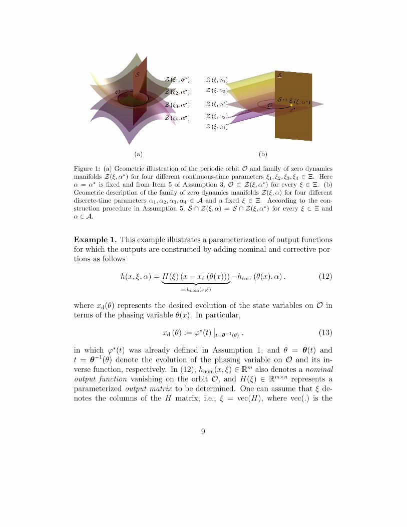
Figure 1: (a) Geometric illustration of the periodic orbit O and family of zero dynamicsmanifolds Z(ξ, α⋆) for four different continuous-time parameters ξ1, ξ2, ξ3, ξ4 ∈ Ξ. Hereα = α⋆ is fixed and from Item 5 of Assumption 3, O ⊂ Z(ξ, α⋆) for every ξ ∈ Ξ. (b)Geometric description of the family of zero dynamics manifolds Z(ξ, α) for four differentdiscrete-time parameters α1, α2, α3, α4 ∈ A and a fixed ξ ∈ Ξ. According to the con-struction procedure in Assumption 5, S ∩ Z(ξ, α) = S ∩ Z(ξ, α⋆) for every ξ ∈ Ξ andα ∈ A.

Example 1. This example illustrates a parameterization of output functionsfor which the outputs are constructed by adding nominal and corrective por-tions as follows

h(x, ξ, α) = H(ξ) (x− xd (θ(x)))︸ ︷︷ ︸

=:hnom(x,ξ)

−hcorr (θ(x), α) , (12)

where xd(θ) represents the desired evolution of the state variables on O interms of the phasing variable θ(x). In particular,

xd (θ) := ϕ⋆(t)∣∣t=θ

−1(θ) , (13)

in which ϕ⋆(t) was already defined in Assumption 1, and θ = θ(t) andt = θ

−1(θ) denote the evolution of the phasing variable on O and its in-verse function, respectively. In (12), hnom(x, ξ) ∈ R

m also denotes a nominaloutput function vanishing on the orbit O, and H(ξ) ∈ R

m×n represents aparameterized output matrix to be determined. One can assume that ξ de-notes the columns of the H matrix, i.e., ξ = vec(H), where vec(.) is the

9

vectorization operator. The corrective term is then defined as

hcorr (θ, α) :=

b (θ, α) , if θ ≤ θth

b (θ, α⋆) , otherwise(14)

to zero the output function (12) right after the switching event (this will beclarified with more details in Section 2.2). To satisfy Items 1, 2, and 5 ofAssumption 3, the function b : R×A → R

m is finally assumed to be w-timesdifferentiable with respect to (θ, α) with the following properties:

1. b(θ, α⋆) ≡ 0 for some α⋆ ∈ A.

2. b(θth, α) =∂b∂θ(θth, α) = · · · = ∂wb

∂θw(θth, α) = 0 for every α ∈ A.

Using these properties, one can easily see that Item 5 of Assumption 3 is sat-isfied. Furthermore, these properties make the piece-wise defined correctivefunction in (14) w-times differentiable with respect to θ which in combinationwith Assumption 2 fulfills Item 1 of Assumption 3.

Now we are in a position to present a diffeomorphism to investigate theevolution of the hybrid system in a set of tangent and transverse coordinates.The following assumption presents a valid change of coordinates for the statespace in which the tangent coordinates for the family of zero dynamics man-ifolds in (11) are assumed to be independent of the value of the continuous-and discrete-time parameters ξ and α.

Assumption 4 (Invariant Tangent Coordinates). There exists a smoothfunction z : X → R

k, referred to as the tangent coordinates, with the propertyLgjz(x) = 0 for all j = 1, · · · , m such that the mapping Ψ : X ×Ξ×A → R

n

by

x = Ψ(x, ξ, α) :=

[z(x)

η(x, ξ, α)

]

(15)

is a diffeomorphism to its image, where

η (x, ξ, α) :=

h(x, ξ, α)Lfh(x, ξ, α)

...Lr−1f h(x, ξ, α)

∈ R

rm. (16)

denotes the transverse coordinates.

10

From the relative degree condition in Item 3 of Assumption 3, one canpresent a valid change of coordinates, parameterized by (ξ, α), to repre-sent the continuous-time portion of the hybrid system in a set of tangentand transverse coordinates [41, Proposition 5.1.2]. However, Assumption 4presents a special structure for the corresponding diffeomorphism by suppos-ing that the tangent coordinates z(x) are independent of the value of theoutput parameters (ξ, α). The motivation for this assumption comes from aset of coordinates introduced in [26, Appendix A] to describe zero dynamicsof underactuated robots. This will help us to simplify the computation of theparameterized Poincare map and the stability analysis in Sections 2.3 and 3.An example of a set of tangent coordinates satisfying this assumption willalso be presented for the numerical results of Section 4. We remark that thetransverse coordinates η(x, ξ, α) in Assumption 4 are free to be parameterizedby the output parameters.

In order to make the family of zero dynamics manifolds Z(ξ, α) attrac-tive and forward invariant under the flow of the closed-loop continuous-timephase, we now employ a family of parameterized nonlinear controllers, arisingfrom the standard I-O linearization technique [41], as follows

Γ (x, ξ, α) := −(LgL

r−1f h (x, ξ, α)

)−1

(

Lrfh (x, ξ, α) +

r−1∑

j=0

kjεr−j

Ljfh (x, ξ, α)

)

,

(17)where ε > 0 and the constants kj for j = 0, 1, · · · , r− 1 are chosen such thatthe monic polynomial χ(λ) := λr + kr−1λ

r−1 + · · · + k0 becomes Hurwitz.Applying the feedback law (17) results in the output dynamics

y(r) +kr−1

εy(r−1) + · · ·+

k0εry = 0 (18)

for which the origin is exponentially stable1. In addition, the output dynam-ics (18) can be written in the following compact equation

η = F (ε) η (19)

1For every ε > 0, λ is a root for χ(λ) = 0 if and only if 1ελ becomes a root for

χ(λ, ε) = λr + kr−1

ελr−1 + · · · + k0

εr= 0. Therefore, χ(λ) is a Hurwitz polynomial if and

only if χ(λ, ε) is Hurwitz.

11

in which F (ε) ∈ Rrm×rm is a Hurwitz matrix with the property limεց0 exp(F (ε) T ⋆) =

0 [42]. The tangent dynamics can then be given by

z = f0 (z, η, ξ, α) , (20)

where [f0 (z, η, ξ, α)

F (ε) η

]

=∂Ψ

∂x(x, ξ, α) f cl (x, ξ, α)

∣∣∣x=Ψ−1(z,η,ξ,α)

and f cl(x, ξ, α) := f(x) + g(x) Γ(x, ξ, α) and Ψ−1(z, η, ξ, α) represent theclosed-loop vector field and inverse of the mapping (15), respectively. Thesuperscript “cl” also stands for the closed-loop system. For later purposes,the family of the zero dynamics manifolds (11) can be rewritten as Z(ξ, α) =(z⊤, η⊤)⊤ | η = 0 for which the parameterized zero dynamics become

z = f0(z, 0, ξ, α). (21)

2.2. Hybrid Invariance

This section investigates the hybrid invariance property of the parame-terized zero dynamics manifolds Z(ξ, α). In particular, we present a set ofparameterized event-based update laws to make the family of zero dynamicsmanifolds hybrid invariant under the flow of the closed-loop hybrid system.For this purpose from Assumption 2, θ(x) is strictly increasing on O. Ac-cording to the construction procedure of the output functions in (10) andthe fact that θth ∈ (θmin, θmax), one can conclude that the periodic orbitO intersects the switching manifold S in the sub-domain θ(x) > θth, i.e.,θ(x⋆) > θth. Thus, there is an open neighborhood B(x⋆) ⊂ N (O) of x⋆

such that for every (x, ξ, α) ∈ B(x⋆)× Ξ×A, θ(x) > θth, and consequently,h(x, ξ, α) = h(x, ξ, α⋆) (see the structure of the output function in (10)).This implies that for every (x, ξ, α) ∈ B(x⋆)×Ξ×A, x ∈ Z(ξ, α) if and onlyif x ∈ Z(ξ, α⋆) (see Fig. 1.b). Now we are in a position to present the hybridinvariance assumption for the family of zero dynamics manifolds.

Assumption 5 (Hybrid Invariance). We assume that for every fixed ξ ∈ Ξ,the family of zero dynamics manifolds Z(ξ, α) has a nonempty and k −1 dimensional intersection with the switching manifold S, shown by S ∩Z(ξ, α⋆), which is independent of the value of the discrete-time parametersα. That is,

S ∩ Z (ξ, α) = S ∩ Z(ξ, α⋆) 6= ∅, ∀α ∈ A (22)

12

(see again Fig. 1.b). We further suppose that the hybrid invariance propertyis satisfied. In particular, there exists a smooth and parameterized event-based update law 2 v(z, ξ) ∈ A such that (1) it maps x⋆ to α⋆ for every ξ ∈ Ξ,i.e.,

v (z (x⋆) , ξ) = α⋆, ∀ξ ∈ Ξ, (23)

and (2) for all x− ∈ S ∩ Z(ξ, α⋆) and ξ ∈ Ξ,

x+ ∈ Z(ξ, α+

), (24)

where x+ = ∆(x−) andα+ = v

(z(x−), ξ). (25)

Remark 1. Assumption 5 has important consequences. First, the diffeo-morphism Ψ, restricted to B(x⋆), becomes independent of the discrete-timeparameters α and can be shown by Ψ(x, ξ, α⋆). This results in the followinglocal image of the switching manifold S under the mapping Ψ(x, ξ, α⋆),

Sξ :=(z⊤, η⊤)⊤ | s (z, η, ξ) = 0

, (26)

where s(z, η, ξ) := s Ψ−1(z, η, ξ, α⋆). Second, the reset map ∆ can locallybe expressed in the (z, η) coordinates as follows

∆(z−, η−, ξ

):=

[∆z (z

−, η−, ξ)

∆η (z−, η−, ξ)

]

:= Ψ(∆(x−), ξ, α+

)∣∣∣x− = Ψ−1

(

z−, η−, ξ, α⋆)

, α+ = v(

z−, ξ)

(27)

in which the subscripts “z” and “η” stand for the z and η coordinates, re-spectively. For later purposes, we remark that Sξ and ∆(z−, η−, ξ) are onlyparameterized by the continuous-time parameters ξ which will affect thestructure of the Jacobian matrix of the Poincare map in Theorem 1.

2.3. Closed-Loop Hybrid Model and Poincare Return Map

By employing the I-O linearizing controller (17) and the event-based up-date law (25), the closed-loop hybrid model becomes

Σcl :

[xα

]

=

[f cl(x, ξ, α)

0

]

, x− /∈ S

[x+

α+

]

=

[∆(x−)

v (z (x−) , ξ)

]

, x− ∈ S,

(28)

2The event-based update law is only parameterized by the continuous-time parameters.

13

where the discrete-time parameters α are kept constant during the continuous-time phase, i.e., α = 0 and are updated according to the event-based lawα+ = v(z(x−), ξ) on the switching manifold S. Here, the continuous-timeparameters ξ are assumed to be constant.

Lemma 1 (Invariant Periodic Orbit). Assume that Assumptions 1-5 aresatisfied. Then, O×α⋆ is a period-one orbit for (28) which is transversal toS×A. Furthermore, this orbit is independent of the value of the continuous-time parameters ξ.

Proof. According to the construction procedure in Item 5 of Assumption3, O ⊂ Z(ξ, α⋆) for all ξ ∈ Ξ. In addition from Item 3 of Assumption3, the decoupling matrix is square and full rank, and the control drivingh(x, ξ, α⋆) to zero is unique on Z(ξ, α⋆) [41, pp. 226]. Hence, the controlΓ(x, ξ, α⋆), restricted to O, becomes independent of ξ. This fact togetherwith Assumption 4 and (23) implies that O×α⋆ is an orbit of (28) for allξ ∈ Ξ. Transversality follows directly from Assumption 1.

For later purposes, the unique solution of the parameterized ODE x =f cl(x, ξ, α) (supposed to be at least C1) with the initial condition x(0) = x0

is denoted by ϕ(t, x0, ξ, α) for all t ≥ 0 in the maximal interval of existence.The time-to-switching function T : X × Ξ×A → R>0 is also defined as thefirst time at which the flow of the ODE intersects the switching manifold S,that is,

T (x0, ξ, α) := inf t > 0 |ϕ (t, x0, ξ, α) ∈ S .

The evolution of the closed-loop hybrid system (28) on the Poincare sectionS ×A can then be described by the following discrete-time system

[x[k + 1]α[k + 1]

]

=

[P (x[k], v (z (x[k]) , ξ) , ξ)

v (z (x[k]) , ξ)

]

, k = 0, 1, · · · , (29)

in which P : S ×A× Ξ → S by

P (x, α, ξ) := ϕ (T (∆(x), ξ, α) ,∆(x), ξ, α) (30)

denotes the parameterized Poincare map. According to the construction pro-cedure in Assumptions 3 and 4, and (23), (x⋆, α⋆) is an invariant fixed pointfor the discrete-time system (29) under the change of the continuous-timeparameters ξ, i.e.,

[P (x⋆, α⋆, ξ)v (z (x⋆) , ξ)

]

=

[x⋆

α⋆

]

, ∀ξ ∈ Ξ. (31)

14

In order to reduce the dimension of the stabilization problem, we now con-sider the discrete-time system (29) in the (z, η, α) coordinates as follows

z[k + 1]η[k + 1]α[k + 1]

=

Pz (z[k], η[k], v (z[k], ξ) , ξ)

Pη (z[k], η[k], v (z[k], ξ) , ξ)v (z[k], ξ)

, (32)

where P (., ., ., ξ) : Sξ ×A → Sξ is defined by3

P (z, η, α, ξ) :=

[Pz (z, η, α, ξ)

Pη (z, η, α, ξ)

]

:= Ψ(P(Ψ−1 (z, η, ξ, α⋆) , α, ξ

), ξ, α⋆

). (33)

Direct calculations shows that (32) is a Poincare map for the following hybridsystem

Σcl :

zηα

=

f0 (z, η, ξ, α)F (ε) η

0

,

[z−

η−

]

/∈ Sξ

z+

η+

α+

=

∆z (z−, η−, ξ)

∆η (z−, η−, ξ)

v (z−, ξ)

,

[z−

η−

]

∈ Sξ,

(34)

for which the Poincare section Sξ × A is parameterized by ξ. Now we arein a position to present the fundamental properties of the closed-loop hybridmodel (34) based on which the main results will be presented in Section 3.

Lemma 2 (Properties of the Closed-Loop Hybrid System). Under Assump-tions 1-5, the following statements are correct.

1. (Invariant Image of the Orbit): The projection of the periodic orbitO under the mapping Ψ(., ξ, α⋆) is independent of the value of thecontinuous-time parameters ξ and can be given by O := Oz × 0,where Oz := z = ϕ⋆

z(t) | t ∈ [0, T ⋆) and

[ϕ⋆z(t)0

]

:= Ψ (ϕ⋆(t), ξ, α⋆) , ∀(t, ξ) ∈ [0, T ⋆]× Ξ. (35)

3In (33), we have made use of the assumption that Ψ and Ψ−1 on B(x⋆)∩S and Sξ donot change by the discrete-time parameters α, respectively (see Remark 1).

15

In particular, (z⋆⊤, 0)⊤ := Ψ(x⋆, ξ, α⋆) is independent of the choice ofξ ∈ Ξ.

2. (Invariant Orbit): For every ξ ∈ Ξ, O × α⋆ is a periodic orbit for(34) which is transversal to Sξ × A. More specifically, the followingindependence properties are satisfied

∂f0∂ξ

(ϕ⋆z(t), 0, ξ, α

⋆) = 0, ∀(t, ξ) ∈ [0, T ⋆]× Ξ (36)

∂s

∂ξ(z⋆, 0, ξ) = 0, ∀ξ ∈ Ξ (37)

∂∆z

∂ξ(z⋆, 0, ξ) = 0, ∀ξ ∈ Ξ (38)

∂∆η

∂ξ(z⋆, 0, ξ) = 0, ∀ξ ∈ Ξ. (39)

3. (Hybrid Invariance): ∆η(z−, 0, ξ) = 0 for all ξ ∈ Ξ and z− in an open

neighborhood of z⋆.

Proof. Part (1): According to Item 5 of Assumption 3 and the constructionprocedure in (16), one can conclude that η(x, ξ, α⋆) = 0 for all (x, ξ) ∈ O×Ξ.In addition from Assumption 4, the tangent coordinates z(x) are independentof the value of ξ. These two facts result in (35).

Part (2): From Lemma 1, O × α⋆ is a transversal periodic orbit for(28) which is independent of the value of ξ. This in combination with Part(1) of Lemma 2 implies that O × α⋆ is also a transversal4 orbit for (34).Equations (36)-(39) are immediate consequences of the invariance propertywith respect to ξ.

Part (3) follows directly from Assumption 5.

3. Main Results

The objective of this section is to present a reduced-order exponential sta-bilization framework to systematically search for continuous-time parametersξ. The state space for the discrete-time system (32) is taken as Sξ×A which isparameterized by ξ. This complicates the computation of the parameterized

4We remark that the transversality is invariant under the valid change of coordinates.

16

Poincare map as well as the stabilization problem when one looks for a set ofcontinuous-time parameters ξ using the optimization framework of (3) and(4). To address these problems, this section introduces an augmented closed-loop hybrid system whose Poincare section is not parameterized by ξ. Nextit presents a asystematic way to numerically compute the Jacobian of thecorresponding parameterized Poincare map. The resultant Jacobian matrixis finally investigated to present a reduced-order stabilization framework.

To achieve the goals of this section, let us consider the following aug-mented system in the (z, η, α, ξ) coordinates

Σcla :

zηα

ξ

=

f0(z, η, ξ, α)F (ε) η

00

,

z−

η−

α−

ξ−

/∈ Sa

z+

η+

α+

ξ+

=

∆z (z−, η−, ξ−)

∆η (z−, η−, ξ−)

v (z−, ξ−)ξ−

,

z−

η−

α−

ξ−

∈ Sa,

(40)

where ξ is now taken as one of the state variables,

Sa :=(z⊤, η⊤, α⊤, ξ⊤)⊤ | s (z, η, ξ) = 0

(41)

denotes an augmented switching manifold, and the subscript “a” stands forthe augmented system. In order to keep ξ constant, the evolution of ξ duringthe continuous- and discrete-time phases of the augmented model (40) isdescribed by ξ = 0 and ξ+ = ξ−, respectively. To study the stabilizationproblem of the periodic orbitO for the closed-loop hybrid system, we considerthe augmented Poincare return map for (40) which is defined as Pa : Sa → Sa

by

Pa (z, η, α, ξ) :=

Pz (z, η, v (z, ξ) , ξ)

Pη (z, η, v (z, ξ) , ξ)v (z, ξ)

ξ

. (42)

The following theorem addresses the properties of the augmented Poincaremap.

Theorem 1 (Properties of the Augmented Poincare Map). Assume thatAssumptions 1-5 are satisfied. Then, the following statements are correct.

17

1. (Augmented Orbit): For every ξ ∈ Ξ, Oa := Oz × 0 × α⋆ × ξ isa periodic orbit for the augmented hybrid system (40). Furthermore,Oa is transversal to Sa.

2. (Augmented Fixed Point): For every ξ ∈ Ξ, (z⋆⊤, 0, α⋆⊤, ξ⊤)⊤ is a fixedpoint of Pa, i.e., the fixed points are not isolated.

3. (Structure of the Augmented Jacobian Matrix): For every ξ ∈ Ξ, theJacobian of the Poincare map Pa, evaluated at (z⋆⊤, 0, α⋆⊤, ξ⊤)⊤, hasthe following structure

DzPz (z⋆, 0, α⋆, ξ) DηPz (z

⋆, 0, α⋆, ξ) 0 0

0 DηPη (z⋆, 0, α⋆, ξ) 0 0

Dzv(z⋆, ξ) 0 0 0

0 0 0 I

. (43)

Remark 2 (Geometric Description). According to the construction proce-dure in (40) and Parts (1) and (2) of Theorem 1, one can present a geometricdescription for the augmented orbit Oa in the state space of the system (40)(see Fig. 2). In this description, the augmented state space and augmentedswitching manifold for Σa are given by R

n×A×Ξ and Sa, respectively. Whenξ changes, the family of augmented orbits can form a cylinder as O×α⋆×Ξ.For a fixed ξ ∈ Ξ, the intersections of the augmented switching manifold Sa

and the cylinder with the hyperplane ξ = const become Sξ and O×α⋆×ξ,respectively. We remark that these intersections coincide with the switchingmanifold and periodic orbit of the closed-loop system Σcl in (34). Item 3of Theorem 1 presents a special structure for the Jacobian linearization ofthe augmented Poincare map in (43) which will simplify the stabilizationproblem in Theorem 2. The problem of exponential stabilization consists offinding the continuous-time parameters ξ such that the intersection of thecylinder O × α⋆×Ξ with the hyperplane ξ = const becomes exponentiallystable for (34).

Proof. Parts (1) and (2) are immediate.Part (3): Let us define the augmented state vector, closed-loop vector

field, reset map, and switching function as xa := (z⊤, η⊤, α⊤, ξ⊤)⊤, fa(xa) :=(f⊤

0 , η⊤F⊤, 0, 0)⊤, ∆a(xa) := (∆⊤

z , ∆⊤η , v

⊤, ξ⊤)⊤, and sa(xa) := s, respec-tively. In addition for a fixed ξ ∈ Ξ, the augmented nominal solution can berepresented by ϕ⋆

a(t) := (ϕ⋆⊤z (t), 0, α⋆⊤, ξ⊤)⊤ for every t ∈ [0, T ⋆]. Next we

define the Jacobian matrix of the augmented closed-loop vector field along

18

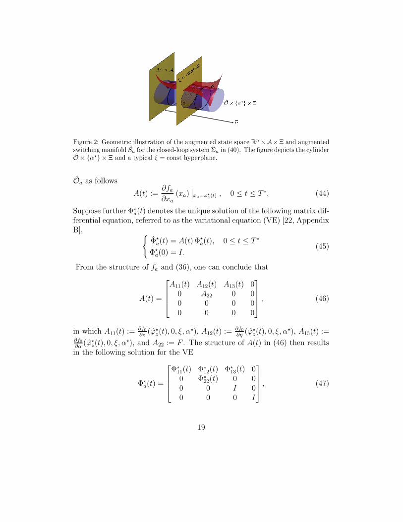
Figure 2: Geometric illustration of the augmented state space Rn×A×Ξ and augmentedswitching manifold Sa for the closed-loop system Σa in (40). The figure depicts the cylinderO × α⋆ × Ξ and a typical ξ = const hyperplane.

Oa as follows

A(t) :=∂fa∂xa

(xa)∣∣xa=ϕ⋆

a(t) , 0 ≤ t ≤ T ⋆. (44)

Suppose further Φ⋆a(t) denotes the unique solution of the following matrix dif-

ferential equation, referred to as the variational equation (VE) [22, AppendixB],

Φ⋆a(t) = A(t) Φ⋆

a(t), 0 ≤ t ≤ T ⋆

Φ⋆a(0) = I.

(45)

From the structure of fa and (36), one can conclude that

A(t) =

A11(t) A12(t) A13(t) 00 A22 0 00 0 0 00 0 0 0

, (46)

in which A11(t) :=∂f0∂z

(ϕ⋆z(t), 0, ξ, α

⋆), A12(t) :=∂f0∂η

(ϕ⋆z(t), 0, ξ, α

⋆), A13(t) :=∂f0∂α

(ϕ⋆z(t), 0, ξ, α

⋆), and A22 := F . The structure of A(t) in (46) then resultsin the following solution for the VE

Φ⋆a(t) =

Φ⋆11(t) Φ⋆

12(t) Φ⋆13(t) 0

0 Φ⋆22(t) 0 0

0 0 I 00 0 0 I

, (47)

19

where

Φ⋆11(t) = A11(t) Φ

⋆11(t), Φ⋆

11(0) = I

Φ⋆12(t) = A11(t) Φ

⋆12(t) + A12(t) Φ

⋆22(t), Φ⋆

12(0) = 0

Φ⋆13(t) = A11(t) Φ

⋆13(t) + A13(t), Φ⋆

13(0) = 0

Φ⋆22(t) = exp(F (ε) t).

We now consider the saltation matrix

Πa := I −fa (x

⋆a)

∂sa∂xa

(x⋆a)

∂sa∂xa

(x⋆a) fa (x

⋆a), (48)

in which x⋆a := (z⋆⊤, 0, α⋆⊤, ξ⊤)⊤ denotes the augmented fixed point. Using

(37), the saltation matrix becomes

Πa =

Π11 Π12 0 00 I 0 00 0 I 00 0 0 I

, (49)

where

Π11 := I −f0 (z

⋆, 0, ξ, α⋆) ∂s∂z

(z⋆, 0, ξ)∂s∂z

(z⋆, 0, ξ) f0 (z⋆, 0, ξ, α⋆)(50)

Π12 := −f0 (z

⋆, 0, ξ, α⋆) ∂s∂η

(z⋆, 0, ξ)∂s∂z

(z⋆, 0, ξ) f0 (z⋆, 0, ξ, α⋆). (51)

From (38), (39), (23), and Item 3 of Lemma 2, the Jacobian of the augmentedreset map, evaluated at x⋆

a, can be expressed as

Υa :=∂∆a

∂xa

(x⋆a) =

Υ11 Υ12 0 00 Υ22 0 0

Υ31 0 0 00 0 0 I

, (52)

in which Υ11 := ∂∆z

∂z(z⋆, 0, ξ), Υ12 := ∂∆z

∂η(z⋆, 0, ξ), Υ22 := ∂∆η

∂η(z⋆, 0, ξ), and

Υ31 := ∂v∂z(z⋆, ξ). Finally, from [22, Appendix D], the Jacobian of the aug-

mented Poincare map, evaluated at the fixed point x⋆a, is given by

DPa (x⋆a) = Πa Φ

⋆a (T

⋆) Υa (53)

20

which in combination with (47), (49), and (52) results in

DzPz (z⋆, 0, α⋆, ξ) = Π11 Φ

⋆11 (T

⋆) Υ11 + Φ⋆13 (T

⋆) Υ31 (54)

DηPz (z⋆, 0, α⋆, ξ) = Π11 Φ

⋆11 (T

⋆) Υ12 + Φ⋆12 (T

⋆) Υ22+Π12Φ⋆22 (T

⋆) Υ22

(55)

DηPη (z⋆, 0, α⋆, ξ) = Φ⋆

22 (T⋆)Υ22 = exp (F (ε) T ⋆)Υ22. (56)

This completes the proof of Part (3).

Remark 3. Equations (54)-(56) together with Part (3) of Theorem 1 presentimportant improvements with respect to [42]. In particular, [42] did not con-sider parameterized hybrid zero dynamics (HZD) manifolds. In addition, itdid not address the effect of the hybrid-invariance event-based controller onthe structure of the Jacobian matrix of the Poincare map. From Part (3) ofTheorem 1, the contribution of the event-based controller on the Jacobianmatrix can now be seen in two different places. The first one is explicitand includes the (3, 1) block of the Jacobian matrix, i.e., Dzv(z

∗, ξ). Thesecond place is implicit and includes the term Π11Φ

⋆13 (T

⋆)Υ31 in (54) (tan-gent coordinates). Finally, (54) presents a systematic approach to computethe Jacobian of the parameterized restricted map as given in the followingcorollary.

Corollary 1 (Numerical Approach for Computing the Parameterized Re-stricted Poincare Map). Consider the parameterized zero dynamics z =f0(z, 0, ξ, α) and let Φ⋆

11(t, ξ) and Φ⋆13(t, ξ) denote the solution of the following

parameterized VEs

Φ⋆11(t, ξ) =

∂f0∂z

(z, 0, ξ, α⋆)∣∣z=ϕ⋆

z(t) Φ⋆11(t, ξ), Φ⋆

11(0, ξ) = I

Φ⋆13(t, ξ) =

∂f0∂z

(z, 0, ξ, α⋆)∣∣z=ϕ⋆

z(t) Φ⋆13(t, ξ) +

∂f0∂α

(z, 0, ξ, α⋆)∣∣z=ϕ⋆

z(t) , Φ⋆13(0, ξ) = 0

for t ∈ [0, T ⋆]. Then, the Jacobian of the parameterized Poincare map along

21

the z-coordinates and restricted to Sξ∩Z(ξ, α⋆) can be computed as follows5

DzPz (z⋆, 0, α⋆, ξ) = πproj(ξ) Π11(ξ)

Φ⋆

11(T⋆, ξ) Υ11(ξ)

︸ ︷︷ ︸

Zero Dynamics Portion

+Φ⋆13(T

⋆, ξ) Υ31(ξ)︸ ︷︷ ︸

Event-based Portion

πlift(ξ),

(57)in which Π11, Υ11, and Υ31 were defined in (50) and (52). In (57), we makeuse of the notation “(ξ)” to highlight the dependence on ξ. Finally, πproj(ξ) ∈R

(k−1)×k and πlift ∈ Rk×(k−1) are parameterized projection and lift matrices

satisfying the following conditions

πproj(ξ) πlift(ξ) = I(k−1)×(k−1) (58)

∂s

∂z(z⋆, 0, ξ) πlift(ξ) = 0. (59)

The following theorem makes use of the results of Theorem 1 and Corol-lary 1 to present the reduced-order stabilization framework.

Theorem 2 (Reduced-Order Stabilization Framework). There exists ε > 0such that for all 0 < ε < ε and ξ ∈ Ξ,

ρ(

DzPz (z⋆, 0, α⋆, ξ)

)

< 1 (60)

implies that

1. Oa = Oz × 0 × α⋆ × ξ is stable for the augmented system (40);and

2. Oz × 0 × α⋆ is exponentially stable for (34).

In our notation, ρ(.) denotes the spectral radius of a matrix.

Proof. See Appendix A.

Remark 4. Theorem 2 reduces the optimization problem (3) and (4) intothe following one

min(ξ,Wz,γ)

J (ξ, γ) (61)

s.t. I(

DzPz (z⋆, 0, α⋆, ξ) ,Wz, γ

)

> 0, (62)

5In (54), DzPz (z⋆, 0, α⋆, ξ) is considered from R

k into Rk. However here, we consider it

from the k− 1 dimensional tangent space T(z⋆,0)Sξ ∩Z(ξ, α⋆) back to T(z⋆,0)Sξ ∩Z(ξ, α⋆).

22

in which Wz = W⊤z ∈ R

(k−1)×(k−1) is a lower-dimensional positive definiteLyapunov matrix. We remark that the optimization problem (61) and (62)

requires p+ k(k−1)2

+ 1 decision variables rather than p+ n(n−1)2

+ 1, requiredfor the original one in (3) and (4).

4. Application to Underactuated 3D Bipedal Walking

Virtual constraints are a set of kinematic relations among generalized co-ordinates enforced asymptotically by continuous-time control inputs [2, 43,7, 35, 36, 44, 45, 46, 28, 47, 48]. They are defined to coordinate the links ofbipedal robots within a stride. In this approach, a set of holonomic outputfunctions y(x) are defined for the continuous-time portion of the hybrid mod-els of bipedal robots and then I-O linearizing controllers [41] are employedto regulate the outputs. Virtual constraint controllers have been numericallyand experimentally validated for 2D and 3D underactuated bipedal robots[46, 28, 16, 49, 26] as well as 2D powered prosthetic legs [45, 44, 50, 51]. Formechanical systems with more than one degree of underactuation, the stabil-ity of walking gaits depends on the choice of virtual constraints [35, 25]. Ourrecent approach [35, 37] applied the optimization problem (3) and (4) for thefull-order hybrid systems to search for stabilizing virtual constraints. Theobjective of this section is to employ the reduced-order optimization frame-work (61) and (62) to systematically look for stabilizing virtual constraintsusing a smaller set of decision variables.

For the purpose of this paper, we consider a parameterized family ofvirtual constrains as follows

y(q, ξ, α) := H(ξ) (q − qd(θ))− hcorr(θ, α), (63)

where q and qd(θ) denote the generalized coordinates of the mechanical sys-tem and their desired evolution on the periodic gait in terms of the phasingvariable θ, respectively. We remark that the virtual constraints in (63) havethe structure of the parameterized output functions presented in Example 1for which the uniform relative degree is 2 (i.e., r = 2) due to the second-ordernature of the Lagrangian continuous-time models. H(ξ) q represents a set ofholonomic variables to be controlled, referred to as the controlled variables.The objective is to search for the output matrix H(ξ), or equivalently thecontrolled variables, to guarantee the exponential stability of periodic walk-ing gaits. The corrective term here is defined in a piece-wise manner as givenin (14) for which b(θ, α) is taken as a Bezier polynomial analogous to [25].

23

4.1. ATRIAS: An Underactuated 3D Bipedal Robot

ATRIAS is an underactuated bipedal robot designed for robust and en-ergy efficient 3D walking. The robot’s structure includes a torso with twoidentical legs terminating in point feet (see Fig. 3). More details about therobot’s model can be found in [26, 52]. Two motors in series with harmonicdrives are used to drive each leg in the sagittal plane. In the frontal plane,each of the hip joints is driven by a motor located in the torso. In total, therobot has 6 brushless DC motors.

The orientation of the torso frame with respect to an inertial world framecan be described by thee Euler angles qzT (yaw), qyT (roll), and qxT (pitch)(see Fig. 3). In the sagittal plane, the angles of the shin and thigh linkswith respect to the torso are denoted by q1R and q2R for the right leg andq1L and q2L for the left leg. The angles of the corresponding harmonic driveswith respect to the torso are then represented by qgr1R, qgr2R, qgr1L, and qgr2L(see again Fig. 3). The torques generated by the sagittal plane DC motorsare also denoted by u1R, u2R, u1L, and u2L. In the frontal plane, the anglesof the right and left hips with respect to the torso are represented by q3Rand q3L, respectively. Finally, u3R and u3L denote the corresponding torquesgenerated by the frontal plane DC motors.

During the single support phase, the robot has 13 DOFs. In particular,the generalized coordinates vector can be expressed as

q :=(q⊤u , q

⊤a

)⊤∈ R

13, (64)

where qu and qa denote the unactuated and actuated DOFs, respectively,defined as follows

qu := (qzT, qyT, qxT, q1R, q2R, q1L, q2L)⊤ ∈ R

7 (65)

qa := (qgr1R, qgr2R, q3R, qgr1L, qgr2L, q3L)⊤ ∈ R

6. (66)

The control input vector can also be given by

u := (u1R, u2R, u3R, u1L, u2L, u3L)⊤ ∈ R

6. (67)

Based on the left-right symmetry, one can present an open-loop hybrid modelwith one continuous-time phase, as given in (6), to describe the 3D walkingmotion of ATRIAS [35, Theorem 4]. In particular, the evolution of the

24

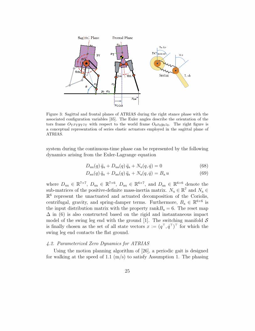
Figure 3: Sagittal and frontal planes of ATRIAS during the right stance phase with theassociated configuration variables [35]. The Euler angles describe the orientation of thetors frame OTxTyTzT with respect to the world frame O0x0y0z0. The right figure isa conceptual representation of series elastic actuators employed in the sagittal plane ofATRIAS.

system during the continuous-time phase can be represented by the followingdynamics arising from the Euler-Lagrange equation

Duu(q) qu +Dua(q) qa +Nu(q, q) = 0 (68)

Dau(q) qu +Daa(q) qa +Na(q, q) = Ba u (69)

where Duu ∈ R7×7, Dua ∈ R

7×6, Dau ∈ R6×7, and Daa ∈ R

6×6 denote thesub-matrices of the positive-definite mass-inertia matrix. Nu ∈ R

7 and Na ∈R

6 represent the unactuated and actuated decomposition of the Coriolis,centrifugal, gravity, and spring-damper terms. Furthermore, Ba ∈ R

6×6 isthe input distribution matrix with the property rankBa = 6. The reset map∆ in (6) is also constructed based on the rigid and instantaneous impactmodel of the swing leg end with the ground [1]. The switching manifold Sis finally chosen as the set of all state vectors x := (q⊤, q⊤)⊤ for which theswing leg end contacts the flat ground.

4.2. Parameterized Zero Dynamics for ATRIAS

Using the motion planning algorithm of [26], a periodic gait is designedfor walking at the speed of 1.1 (m/s) to satisfy Assumption 1. The phasing

25

variable θ is then defined as the angle of the virtual line connecting the stanceleg end to the hip joint in the sagittal plane to fulfill Assumption 2 (see Fig.3). For the ATRIAS structure, θ is only a function of unactuated coordinatesand can be given by θ = θ(qu). The virtual constraints in (63) can then bedecomposed as follows

y(q, ξ, α) =[Hu(ξ) Ha(ξ)

][qu − qud(θ)qa − qad(θ)

]

− hcorr(θ, α)

= 0,

(70)

where Hu(ξ) ∈ R6×7 and Ha(ξ) ∈ R

6×6 are the corresponding sub-matrices ofH(ξ) with the assumption rankHa(ξ) = 6 for every ξ ∈ Ξ. In addition, qud(θ)and qad(θ) denote the desired evolutions of the unactuated and actuatedcoordinates on the orbit O in terms of θ, respectively. From (70), one canobtain the evolution of the actuated coordinates on the parameterized zerodynamics manifold Z(ξ, α) in terms of (qu, ξ, α) as follows

qa = qad(θ)−H−1a (ξ)Hu(ξ) (qu − qud(θ)) +H−1

a (ξ) hcorr(θ, α)

=: qad(qu, ξ, α)(71)

which results in the position lift map

q =

[qu

qad(qu, ξ, α)

]

=: qd(qu, ξ, α). (72)

Substituting (71) and (72) in (68) then results in the following 14-dimensionalparameterized zero dynamics

Dzero(qu, ξ, α) qu +Nzero(qu, qu, ξ, α) = 0, (73)

where

Dzero(qu, ξ, α) := Duu (qd(qu, ξ, α))

+Dua (qd(qu, ξ, α))∂qad∂qu

(qu, ξ, α)

Nzero(qu, qu, ξ, α) := Nu

(

qd(qu, ξ, α), ˙qd(qu, qu, ξ, α))

+Dua (qd(qu, ξ, α))∂

∂qu

(∂qad∂qu

(qu, ξ, α) qu

)

qu.

Based on (73), the tangent coordinates can be chosen as z(x) := (q⊤u , q⊤u )

⊤ ∈R

14 to satisfy Assumption 4. Finally for the ATRIAS structure, we remarkthat the full and restricted Poincare maps are 25- and 13-dimensional, re-spectively.

26

4.3. Numerical Results

For bipedal robots with yaw motion, there are two kinds of stabilityduring waling: full-state stability and stability-modulo yaw. The stabilitymodulo yaw refers to the stability in X \ S1, where S

1 := [0, 2π) denotes theunit circle [5, 53] and “\” represents the set difference. We will apply thereduced-order framework for the stability modulo yaw and full-state stabilityin Sections 4.3.1 and 4.3.2, respectively. To solve the optimization problem(61) and (62), we employ the bilinear matrix inequality (BMI) algorithmdeveloped in [35]. The algorithm is based on the sensitivity analysis andBMIs for which the cost function is chosen as

J (ξ, γ) = −wγ +1

2‖ξ − ξ⋆‖22 , (74)

where ξ⋆ represents a nominal set of continuous-time parameters and w > 0is a weighting factor. In addition, the algorithm approximates the nonlinearmatrix inequality (62) by a BMI based on its Taylor series expansion aroundξ⋆. The cost function (74) tries to improve the convergence rate while keepingthe continuous-time parameters close enough to the nominal ones to havea good approximation for the Taylor series. To numerically solve the BMIalgorithm of [35], we then employ the PENBMI solver from TOMLAB [54, 55]integrated with the MATLAB environment through the YALMIP [56]. Forthe purpose of this paper, the nominal parameters ξ⋆, or equivalently thenominal controlled variables, are chosen as

H⋆ q =

12(qgr1R + qgr2R)

12(qgr1L + qgr2L)qgr2R − qgr1Rqgr2L − qgr1L

q3R−qyT + q3L

. (75)

The first two components of the controlled variables in (75) represent the legangles for the right and left legs. The leg angle is defined as the angle betweenthe torso and the virtual line connecting the hip joint to the leg end. Weremark that for the ATRIAS structure, the legs are actuated through springsand hence, the leg angles are defined at the outputs of the harmonic drives.The third and fourth components of the controlled variables in (75) are thentaken as the right and left knee angles, respectively. The fifth and sixth

27

components are finally defined in the frontal plane. In particular, the fifthcomponent represents the stance hip angle, whereas the sixth component isdefined as the absolute swing hip angle.

4.3.1. Stability Modulo Yaw

Corresponding to the nominal controlled variables given in (75), thedominant eigenvalues of the 13-dimensional restricted Poincare map become−1.3060,−1.000, 0.8815,−0.1221 and consequently, the gait is not stable.From [35], the eigenvalue −1 corresponds to the yaw coordinates. We haveobserved that the first four components of the controlled variables in (75) canstabilize walking gaits for the planar (i.e., 2D) model of ATRIAS [26]. Toimprove the stability of the gait, one can then focus on the lateral stability.For this purpose, we let ξ = (ξ1, · · · , ξ6)⊤ ∈ R

6 only parameterize the secondcolumn of the output matrix H that corresponds to the torso roll angle qyT.In particular, we parameterize the output matrix as follows

H(ξ) = H⋆ +6∑

i=1

Ei,2 ξi, (76)

where for every i ∈ 1, 2, · · · , 6, Ei,2 ∈ R6×13 is a matrix whose elements are

zero except the (i, 2) component. The reduced-order optimization framework(61) and (62) then requires 6+ 14×13

2+1 = 98 decision variables, whereas the

original one in (3) and (4) requires 6 + 26×252

+ 1 = 332 variables (i.e. 70%decrease in the number of decision variables). A local optimal solution forthe BMI algorithm is numerically computed as follows

H(ξ) q =

12(qgr1R + qgr2R)

12(qgr1L + qgr2L)qgr2R − qgr1Rqgr2L − qgr1L

q3R−qyT + q3L

+

−0.55740.4878−0.01620.0735−0.2613−0.3884

︸ ︷︷ ︸

ξ

qyT (77)

for which the dominant eigenvalues of the restricted Poincare map become−1.0000, 0.7067,−0.1577±0.5296i. Hence, the optimal controlled variablesin (77) exponentially stabilize the gait modulo yaw. Figure 4 depicts thephase portraits of the closed-loop hybrid system during 100 consecutive steps.

28

(rad)0 0.02 0.04 0.06 0.08

(rad/s)

-0.2

-0.1

0

0.1

0.2

0.3Yaw

(rad)-0.05 -0.04 -0.03 -0.02 -0.01 0 0.01 0.02 0.03

(rad/s)

-0.6

-0.4

-0.2

0

0.2

0.4

0.6

Roll

(rad)0 0.02 0.04 0.06 0.08 0.1

(rad/s)

-1

-0.5

0

0.5

1 Pitch

(rad)2.4 2.45 2.5 2.55 2.6 2.65 2.7 2.75 2.8 2.85

(rad/s)

-4

-3

-2

-1

0

1

2

3 q3R

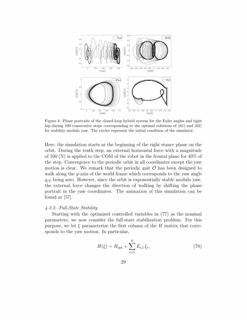
Figure 4: Phase portraits of the closed-loop hybrid system for the Euler angles and righthip during 100 consecutive steps corresponding to the optimal solutions of (61) and (62)for stability modulo yaw. The circles represent the initial condition of the simulator.

Here, the simulation starts at the beginning of the right stance phase on theorbit. During the tenth step, an external horizontal force with a magnitudeof 100 (N) is applied to the COM of the robot in the frontal plane for 40% ofthe step. Convergence to the periodic orbit in all coordinates except the yawmotion is clear. We remark that the periodic gait O has been designed towalk along the y-axis of the world frame which corresponds to the yaw angleqzT being zero. However, since the orbit is exponentially stable modulo yaw,the external force changes the direction of walking by shifting the phaseportrait in the yaw coordinates. The animation of this simulation can befound at [57].

4.3.2. Full-State Stability

Starting with the optimized controlled variables in (77) as the nominalparameters, we now consider the full-state stabilization problem. For thispurpose, we let ξ parameterize the first column of the H matrix that corre-sponds to the yaw motion. In particular,

H(ξ) = Hopt +

6∑

i=1

Ei,1 ξi, (78)

29

where Hopt represents the output matrix obtained in (77) for stability moduloyaw. Furthermore for every i ∈ 1, 2, · · · , 6, Ei,1 ∈ R

6×13 is a matrix whoseelements are zero except the (i, 1) component. For this set of output matrices,the optimal controlled variables become

H(ξ) q =

12(qgr1R + qgr2R)

12(qgr1L + qgr2L)qgr2R − qgr1Rqgr2L − qgr1L

q3R−qyT + q3L

+

−0.55740.4878−0.01620.0735−0.2613−0.3884

qyT +

0.2697−0.1641−0.0266−0.0130−0.1375−0.0266

︸ ︷︷ ︸

ξ

qzT (79)

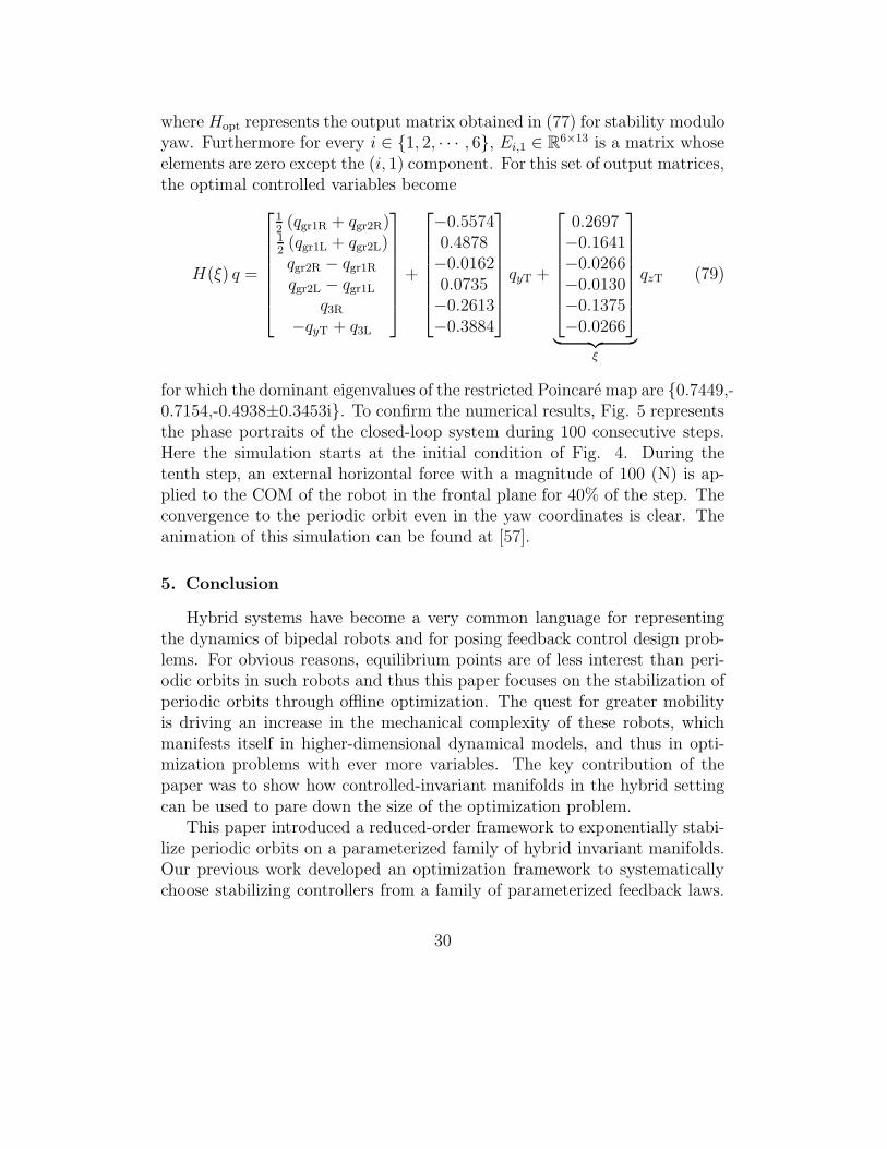
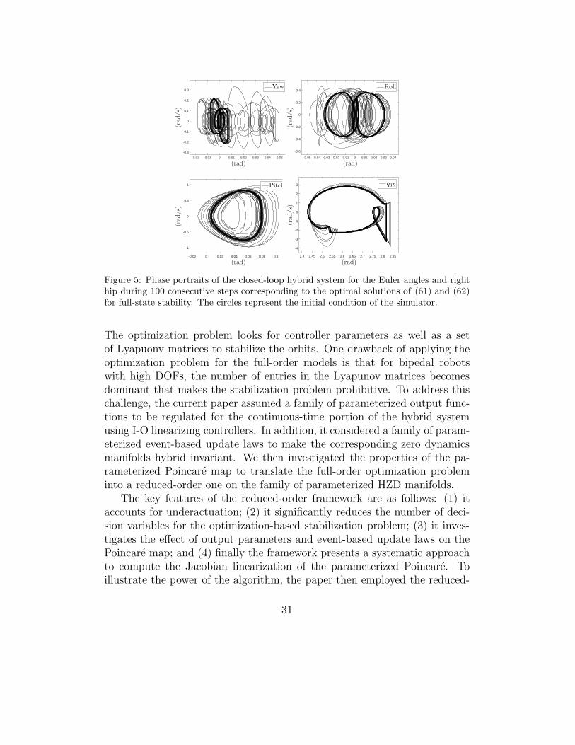
for which the dominant eigenvalues of the restricted Poincare map are 0.7449,-0.7154,-0.4938±0.3453i. To confirm the numerical results, Fig. 5 representsthe phase portraits of the closed-loop system during 100 consecutive steps.Here the simulation starts at the initial condition of Fig. 4. During thetenth step, an external horizontal force with a magnitude of 100 (N) is ap-plied to the COM of the robot in the frontal plane for 40% of the step. Theconvergence to the periodic orbit even in the yaw coordinates is clear. Theanimation of this simulation can be found at [57].

5. Conclusion

Hybrid systems have become a very common language for representingthe dynamics of bipedal robots and for posing feedback control design prob-lems. For obvious reasons, equilibrium points are of less interest than peri-odic orbits in such robots and thus this paper focuses on the stabilization ofperiodic orbits through offline optimization. The quest for greater mobilityis driving an increase in the mechanical complexity of these robots, whichmanifests itself in higher-dimensional dynamical models, and thus in opti-mization problems with ever more variables. The key contribution of thepaper was to show how controlled-invariant manifolds in the hybrid settingcan be used to pare down the size of the optimization problem.

This paper introduced a reduced-order framework to exponentially stabi-lize periodic orbits on a parameterized family of hybrid invariant manifolds.Our previous work developed an optimization framework to systematicallychoose stabilizing controllers from a family of parameterized feedback laws.

30

(rad)-0.02 -0.01 0 0.01 0.02 0.03 0.04 0.05

(rad/s)

-0.3

-0.2

-0.1

0

0.1

0.2

0.3Yaw

(rad)-0.05 -0.04 -0.03 -0.02 -0.01 0 0.01 0.02 0.03 0.04

(rad/s)

-0.6

-0.4

-0.2

0

0.2

0.4Roll

(rad)-0.02 0 0.02 0.04 0.06 0.08 0.1

(rad/s)

-1

-0.5

0

0.5

1 Pitch

(rad)2.4 2.45 2.5 2.55 2.6 2.65 2.7 2.75 2.8 2.85

(rad/s)

-4

-3

-2

-1

0

1

2

3 q3R

Figure 5: Phase portraits of the closed-loop hybrid system for the Euler angles and righthip during 100 consecutive steps corresponding to the optimal solutions of (61) and (62)for full-state stability. The circles represent the initial condition of the simulator.

The optimization problem looks for controller parameters as well as a setof Lyapuonv matrices to stabilize the orbits. One drawback of applying theoptimization problem for the full-order models is that for bipedal robotswith high DOFs, the number of entries in the Lyapunov matrices becomesdominant that makes the stabilization problem prohibitive. To address thischallenge, the current paper assumed a family of parameterized output func-tions to be regulated for the continuous-time portion of the hybrid systemusing I-O linearizing controllers. In addition, it considered a family of param-eterized event-based update laws to make the corresponding zero dynamicsmanifolds hybrid invariant. We then investigated the properties of the pa-rameterized Poincare map to translate the full-order optimization probleminto a reduced-order one on the family of parameterized HZD manifolds.

The key features of the reduced-order framework are as follows: (1) itaccounts for underactuation; (2) it significantly reduces the number of deci-sion variables for the optimization-based stabilization problem; (3) it inves-tigates the effect of output parameters and event-based update laws on thePoincare map; and (4) finally the framework presents a systematic approachto compute the Jacobian linearization of the parameterized Poincare. Toillustrate the power of the algorithm, the paper then employed the reduced-

31

order framework to systematically design stabilizing I-O linearizing controllerfor walking gaits of a 3D bipedal robot with 13 DOFs and 7 degrees of un-deractuation.

Appendix A. Proof of Theorem 2

By defining x1 := (z⊤, η⊤, α⊤)⊤ and x2 := ξ, the augmented hybrid sys-tem (40) can be rewritten in the following compact form

Σcla :

[x1

x2

]

=

[f1 (x1, x2)

0

]

,

[x−1

x−2

]

/∈ Sa

[x+1

x+2

]

=

[∆1

(x−1 , x

−2

)

x−2

]

,

[x−1

x−2

]

∈ Sa,

(A.1)

where f1 := (f⊤0 , η

⊤F⊤, 0)⊤ and ∆1 := (∆⊤z , ∆

⊤η , v

⊤)⊤. Furthermore for every

x2, O1×x2 is a period-one orbit of (A.1), in which O1 := Oz×0×α⋆.Using this new notation, the Jacobian of the Poincare map in (43) can bewritten as [

A11 00 I

]

,

where

A11 :=

DzPz (z⋆, 0, α⋆, ξ) DηPz (z

⋆, 0, α⋆, ξ) 0

0 DηPη (z⋆, 0, α⋆, ξ) 0

Dzv(z⋆, ξ) 0 0

.

Analogous to the analysis of [42], limεց0DηPη(z⋆, 0, α⋆, ξ) = limεց0 exp(F (ε)T ⋆)Υ22 =

0, and hence from continuity of A11 with respect to ε, there is ε > 0 such thatthe dominant eigenvalues of A11 are determined by those of DzPz (z

⋆, ξ, α⋆, 0)for all 0 < ε < ε. This fact in combination with (60) implies that A11 is Schurstable, i.e., all eigenvalues of A11 lie inside the unit circle. Next, the decen-tralized structure of the augmented Poincare return map on Sa as

[x1[k + 1]x2[k + 1]

]

=

[P1 (x1[k], x2[k])

x2[k]

]

guarantees the stability of the fixed point (x⋆⊤1 , x⊤

2 )⊤ for the fixed x2 = ξ,

where P1 := (P⊤z , P⊤

η , v⊤)⊤ and x⋆1 := (z⋆⊤, 0, α⋆⊤)⊤. In addition, x⋆

1 isexponentially stable for x1[k + 1] = P1(x1[k], x2). Now, let us take a point(x⊤

10, x⊤20)

⊤ ∈ Sa and denote the solution of the hybrid system, starting from

32

the initial condition (∆⊤1 (x10, x20), x

⊤20)

⊤, by (ϕ⊤1 (t), ϕ

⊤2 (t))

⊤. Suppose furtherthat t1 represents the first time at which the solution intersects Sa. Thenapplying inequality (C.6) of [58] implies that

sup0≤t≤t1

dist

([ϕ1(t)ϕ2(t)

]

,O1 × x2

)

≤ L

∥∥∥∥

[x10 − x⋆

1

x20 − x2

]∥∥∥∥

≤ L ‖x10 − x⋆1‖+ L ‖x20 − x2‖ (A.2)

for some L > 0. Finally, one can apply the ǫ-δ requirements to show that x⋆1

being exponentially stable for x1[k + 1] = P1(x1[k], x2) implies O1 × x2 isstable for (A.1). In particular for every ǫ > 0, there is δ > 0 such that

∥∥∥∥

[x10 − x⋆

1

x20 − x2

]∥∥∥∥< δ

results in

dist

([ϕ1(t)ϕ2(t)

]

,O1 × x2

)

< ǫ.

This completes the proof of Part (1). For Part (2) when x20 is set to x2,ϕ2(t) ≡ x2 and hence, the inequality (A.2) reduces to

sup0≤t≤t1

dist (ϕ1(t),O1) ≤ L ‖x10 − x⋆1‖

which in turn guarantees the exponential stability of O1 for (34).

Acknowledgments

The work of K. Akbari Hamed was partially supported by the Centerfor Sensorimotor Neural Engineering (CSNE) that is an NSF EngineeringResearch Center. The work of J. W. Grizzle was supported by NSF GrantsECCS-1343720 and NRI-1525006.

References

[1] Y. Hurmuzlu, D. B. Marghitu, Rigid body collisions of pla-nar kinematic chains with multiple contact points, The In-ternational Journal of Robotics Research 13 (1) (1994) 82–92.doi:10.1177/027836499401300106.

33

[2] J. Grizzle, G. Abba, F. Plestan, Asymptotically stable walking for bipedrobots: analysis via systems with impulse effects, Automatic Control,IEEE Transactions on 46 (1) (2001) 51–64. doi:10.1109/9.898695.

[3] G. Song, M. Zefran, Underactuated dynamic three-dimensional bipedalwalking, in: Robotics and Automation. Proceedings IEEE InternationalConference on, 2006, pp. 854–859. doi:10.1109/ROBOT.2006.1641816.

[4] J. W. Grizzle, C. Chevallereau, R. W. Sinnet, A. D. Ames, Models,feedback control, and open problems of 3D bipedal robotic walking,Automatica 50 (8) (2014) 1955–1988.

[5] M. Spong, F. Bullo, Controlled symmetries and passive walking, Au-tomatic Control, IEEE Transactions on 50 (7) (2005) 1025–1031.doi:10.1109/TAC.2005.851449.

[6] M. Spong, J. Holm, D. Lee, Passivity-based control of bipedal loco-motion, Robotics Automation Magazine, IEEE 14 (2) (2007) 30–40.doi:10.1109/MRA.2007.380638.

[7] A. Ames, Human-inspired control of bipedal walking robots, Au-tomatic Control, IEEE Transactions on 59 (5) (2014) 1115–1130.doi:10.1109/TAC.2014.2299342.

[8] A. Ames, K. Galloway, K. Sreenath, J. Grizzle, Rapidly exponen-tially stabilizing control Lyapunov functions and hybrid zero dynam-ics, Automatic Control, IEEE Transactions on 59 (4) (2014) 876–891.doi:10.1109/TAC.2014.2299335.

[9] R. Gregg, L. Righetti, Controlled reduction with unactuated cyclic vari-ables: Application to 3D bipedal walking with passive yaw rotation,Automatic Control, IEEE Transactions on 58 (10) (2013) 2679–2685.doi:10.1109/TAC.2013.2256011.

[10] R. Gregg, A. Tilton, S. Candido, T. Bretl, M. Spong, Control andplanning of 3-D dynamic walking with asymptotically stable gaitprimitives, Robotics, IEEE Transactions on 28 (6) (2012) 1415–1423.doi:10.1109/TRO.2012.2210484.

34

[11] K. Byl, R. Tedrake, Approximate optimal control of the compass gait onrough terrain, in: Robotics and Automation. IEEE International Con-ference on, 2008, pp. 1258–1263. doi:10.1109/ROBOT.2008.4543376.

[12] C. Saglam, K. Byl, Switching policies for metastable walking, in: Deci-sion and Control, IEEE 52nd Annual Conference on, 2013, pp. 977–983.doi:10.1109/CDC.2013.6760009.

[13] H. Dai, R. Tedrake, L2-gain optimization for robust bipedal walkingon unknown terrain, in: Robotics and Automation, IEEE InternationalConference on, 2013, pp. 3116–3123. doi:10.1109/ICRA.2013.6631010.

[14] I. R. Manchester, U. Mettin, F. Iida, R. Tedrake, Stable dynamic walk-ing over uneven terrain, The International Journal of Robotics Research30 (3) (2011) 265–279. doi:10.1177/0278364910395339.

[15] A. Shiriaev, L. Freidovich, S. Gusev, Transverse linearization for con-trolled mechanical systems with several passive degrees of freedom,Automatic Control, IEEE Transactions on 55 (4) (2010) 893–906.doi:10.1109/TAC.2010.2042000.

[16] A. E. Martin, D. C. Post, J. P. Schmiedeler, The effects of foot geomet-ric properties on the gait of planar bipeds walking under HZD-basedcontrol, The International Journal of Robotics Research 33 (12) (2014)1530–1543. doi:10.1177/0278364914532391.

[17] C. D. Remy, Optimal exploitation of natural dynamics in legged loco-motion, Ph.D. thesis, ETH Zurich (2011).

[18] W. Haddad, V. Chellaboina, S. Nersesov, Impulsive and Hybrid Dynam-ical Systems: Stability, Dissipativity, and Control, Princeton UniversityPress, 2006.

[19] R. Goebel, R. Sanfelice, A. Teel, Hybrid Dynamical Systems: Modeling,Stability, and Robustness, Princeton University Press, 2012.

[20] D. Bainov, P. Simeonov, Systems With Impulse Effect: Stability, Theoryand Applications, Ellis Horwood Ltd, 1989.

[21] H. Ye, A. Michel, L. Hou, Stability theory for hybrid dynamical sys-tems, Automatic Control, IEEE Transactions on 43 (4) (1998) 461–474.doi:10.1109/9.664149.

35

[22] T. Parker, L. Chua, Practical Numerical Algorithms for Chaotic Sys-tems, Springer, 1989.

[23] S. Burden, S. Revzen, S. Sastry, Model reduction near periodic orbits ofhybrid dynamical systems, Automatic Control, IEEE Transactions onto appear. doi:10.1109/TAC.2015.2411971.

[24] J. W. Grizzle, Remarks on event-based stabilization of periodic orbitsin systems with impulse effects, in: Second International Symposium onCommunication, Control and Signal Processing, 2006.

[25] C. Chevallereau, J. Grizzle, C.-L. Shih, Asymptotically Stable Walk-ing of a Five-Link Underactuated 3-D Bipedal Robot, Robotics, IEEETransactions on 25 (1) (2009) 37–50. doi:10.1109/TRO.2008.2010366.

[26] A. Ramezani, J. Hurst, K. Akbai Hamed, J. Grizzle, Performance analy-sis and feedback control of ATRIAS, a three-dimensional bipedal robot,Journal of Dynamic Systems, Measurement, and Control December,ASME 136 (2). doi:10.1115/1.4025693.

[27] K. Akbari Hamed, J. Grizzle, Event-based stabilization of peri-odic orbits for underactuated 3-D bipedal robots with left-rightsymmetry, Robotics, IEEE Transactions on 30 (2) (2014) 365–381.doi:10.1109/TRO.2013.2287831.

[28] K. Sreenath, H.-W. Park, I. Poulakakis, J. Grizzle, Embedding activeforce control within the compliant hybrid zero dynamics to achieve sta-ble, fast running on mabel, The International Journal of Robotics Re-search 32 (3) (2013) 324–345. doi:10.1177/0278364912473344.

[29] M. H. Raibert, Legged robots, Communications of the ACM 29 (6)(1986) 499514.

[30] M. Buehler, D. E. Koditschek, P. J. Kindlmann, Planningand control of robotic juggling and catching tasks, The Inter-national Journal of Robotics Research 13 (12) (1994) 101–118.doi:10.1177/027836499401300201.

[31] S. G. Carver, N. J. Cowan, J. M. Guckenheimer, Lateral stability of thespring-mass hopper suggests a two-step control strategy for running,Chaos 19 (2) (2009) 026106. doi:10.1063/1.3127577.

36

[32] M. M. Ankarali, U. Saranli, Control of underactuated planar pronk-ing through an embedded spring-mass hopper template, AutonomousRobots 30 (2) (2011) 217–231.

[33] J. Seipel, P. Holmes, A simple model for clock-actuated legged locomo-tion, Regular and Chaotic Dynamics 12 (5) (2007) 502–520.

[34] A. Seyfarth, H. Geyer, H. Herr, Swing-leg retraction: a simple controlmodel for stable running, The Journal of Experimental Biology 206 (15)(2003) 2547–2555. doi:10.1242/jeb.00463.

[35] K. Akbari Hamed, B. Buss, J. Grizzle, Exponentially stabilizingcontinuous-time controllers for periodic orbits of hybrid systems: Ap-plication to bipedal locomotion with ground height variations, TheInternational Journal of Robotics Research (2015) published online-doi:10.1177/0278364915593400.

[36] K. Akbari Hamed, B. Buss, J. Grizzle, Continuous-time controllersfor stabilizing periodic orbits of hybrid systems: Application toan underactuated 3D bipedal robot, in: Decision and Control(CDC), 2014 IEEE 53rd Annual Conference on, 2014, pp. 1507–1513.doi:10.1109/CDC.2014.7039613.

[37] K. Akbari Hamed, J. Grizzle, Iterative robust stabilization algorithmfor periodic orbits of hybrid dynamical systems: Application to bipedalrunning, in: The IFAC Conference on Analysis and Design of HybridSystems, 2015, accepted to appear.

[38] B. G. Buss, K. Akbari Hamed, B. A. Griffin, J. W. Grizzle, Experimentalresults for 3D bipedal robot walking based on systematic optimizationof virtual constraints, in: The 2016 American Control Conference, 2016,accepted to appear.

[39] Dynamic Leg Locomotion YouTube Channel, MARLO: Dynamic 3Dwalking based on HZD gait design and BMI constraint selection (2015).URL https://www.youtube.com/watch?v=5ms5DtPNwHo

[40] M. Diehl, K. Mombaur, D. Noll, Stability optimization of hybrid periodicsystems via a smooth criterion, Automatic Control, IEEE Transactionson 54 (8) (2009) 1875–1880. doi:10.1109/TAC.2009.2020669.

37

[41] A. Isidori, Nonlinear Control Systems, Springer; 3rd edition, 1995.

[42] B. Morris, J. Grizzle, Hybrid invariant manifolds in systems with im-pulse effects with application to periodic locomotion in bipedal robots,Automatic Control, IEEE Transactions on 54 (8) (2009) 1751–1764.doi:10.1109/TAC.2009.2024563.

[43] E. Westervelt, J. Grizzle, D. Koditschek, Hybrid zero dynamics of planarbiped walkers, Automatic Control, IEEE Transactions on 48 (1) (2003)42–56. doi:10.1109/TAC.2002.806653.

[44] R. Gregg, J. Sensinger, Towards biomimetic virtual constraint controlof a powered prosthetic leg, Control Systems Technology, IEEE Trans-actions on 22 (1) (2014) 246–254. doi:10.1109/TCST.2012.2236840.

[45] R. Gregg, T. Lenzi, L. Hargrove, J. Sensinger, Virtual constraint con-trol of a powered prosthetic leg: From simulation to experiments withtransfemoral amputees, Robotics, IEEE Transactions on 30 (6) (2014)1455–1471. doi:10.1109/TRO.2014.2361937.

[46] C. Chevallereau, G. Abba, Y. Aoustin, F. Plestan, E. Westervelt,C. Canudas-de Wit, J. Grizzle, RABBIT: a testbed for advanced con-trol theory, Control Systems Magazine, IEEE 23 (5) (2003) 57–79.doi:10.1109/MCS.2003.1234651.

[47] M. Maggiore, L. Consolini, Virtual holonomic constraints for Euler La-grange systems, Automatic Control, IEEE Transactions on 58 (4) (2013)1001–1008. doi:10.1109/TAC.2012.2215538.

[48] A. Shiriaev, A. Sandberg, C. Canudas de Wit, Motion planning andfeedback stabilization of periodic orbits for an acrobot, in: Decision andControl. 43rd IEEE Conference on, Vol. 1, 2004, pp. 290–295 Vol.1.doi:10.1109/CDC.2004.1428645.

[49] J. Lack, M. Powell, A. Ames, Planar multi-contact bipedal walking usinghybrid zero dynamics, in: Robotics and Automation, IEEE InternationalConference on, 2014, pp. 2582–2588. doi:10.1109/ICRA.2014.6907229.

[50] A. Martin, R. Gregg, Hybrid invariance and stability of a feedback lin-earizing controller for powered prostheses, in: American Control Con-ference, 2015, pp. 4670–4676.

38

[51] H. Zhao, J. Horn, J. Reher, V. Paredes, A. D. Ames, A hybrid systemsand optimization-based control approach to realizing multi-contact lo-comotion on transfemoral prostheses, in: 54th IEEE Conference on De-cision and Control, Osaka, Japan, 2015.

[52] Dynamic Leg Locomotion at University of Michigan,https://sites.google.com/site/atrias21/ (2013).

[53] C.-L. Shih, J. W. Grizzle, C. Chevallereau, From stable walking to steer-ing of a 3D bipedal robot with passive point feet, Robotica 30 (2012)1119–1130. doi:10.1017/S026357471100138X.

[54] D. Henrion, J. Lofberg, M. Kocvara, M. Stingl, Solving polynomial staticoutput feedback problems with PENBMI, in: Decision and Control,and European Control Conference. 44th IEEE Conference on, 2005, pp.7581–7586. doi:10.1109/CDC.2005.1583385.

[55] TOMLAB optimization, http://tomopt.com/tomlab/.

[56] J. Lofberg, YALMIP: a toolbox for modeling and optimization in MAT-LAB, in: Computer Aided Control Systems Design, 2004 IEEE Inter-national Symposium on, 2004, pp. 284–289.

[57] K. Akbari Hamed’s YouTube Channel, Reduced-Order Framework forStabilization of Periodic Orbits on Parameterized HZD Manifolds,

https://www.youtube.com/watch?v=e_DlqFFCnf0&feature=youtu.be

(2016).

[58] E. Westervelt, J. Grizzle, C. Chevallereau, J. Choi, B. Morris, FeedbackControl of Dynamic Bipedal Robot Locomotion, Taylor & Francis/CRC,2007.

39