REDUCED GRADIENT BUBBLE MODELWITH BASIS AND COMPARISONS

NAUI Technical Series 8

Bruce R. Wienke and Timothy R. O’LearyNAUI Technical Diving Operations

Tampa, Florida 33619

INTRODUCTION

OverviewTables and meters employ deterministic staging algorithms, with models broadly categorized as Haldane (dissolved

phase) or as bubble (combination of dissolved and free phases). The Reduced Gradient Bubble Model (RGBM) isone such dual phase model developed for a very wide spectrum of diving activities (bounce, altitude, decompression,saturation, repetitive, multiday). Over appropriate diving ranges and exposures, the general features of the RGBM canbe retrofitted to any more limited model, like a Haldane dissolved gas model, across nonstop time limits and criticalstaging parameters (Workman Mvalues, Buhlmann a, b) This extended writeup addresses the reduction and linkage ofthe RGBM to the ZHL (Haldane) Buhlmann algorithm, using the ZHL desired nonstop limits and critical tensions. Theprocess involves both profile and parameter fitting in the synthesis, requiring fairly powerful computers. All techniquesand model essentials are contained in this document, however, only the fundamental relationships are presented anddiscussed for simplicity and (hopefully) clarity. The full iterative RGBM is described and discussed, and is, of course,the basis of the recently released NAUI ranged trimix, heliox, and nitrox tables for recreational and technical diving,and model imbedded in the ABYSS software suite of decompression staging platforms.

We first discuss DCI risk and coupled statistics, then return to specific description of the RGBM, and the algorithmused in diving applications. The next section details the RGBM/ZHL and synthesis linking the Haldane (ZHL) and phase(RGBM) models. A discussion of the mulitdiving fractions, f , and their relationship to the RGBM and ZHL algorithmsis also sketched. The first half is general in content, focusing on decompression risk and the full blown RGBM. Thesecond half is specific to the ZHL implementation of the RGBM, using the ZHL critical parameters and exposuretimes, and details all linkages to the RGBM, profile and parameter fitting, and data employed in coupling analysis, andcontrasts layman differences between phase (RGBM/ZHL and RGBM) and dissolved gas models, focusing on diveware(ABYSS) and decometer (Haldane) predictions for test profiles.

Models And DataDiving models address the coupled issues of gas uptake and elimination, bubbles, and pressure changes in different

computational frameworks. Application of a computational model to staging divers is called a diving algorithm. TheRGBM is a modern one, treating the many facets of gas dynamics in tissue and blood consistently. Though the system-atics of gas exchange, nucleation, bubble growth or collapse, and decompression are so complicated that theories onlyreflect pieces of the DCI puzzle, the risk and statistics of decompressing divers are straightforward. And folding of DCIrisk and statistics over data and model assumptions is perhaps the best means to safety and model closure.

STATISTICS AND RISK ANALYSIS

Decompression Risk And StatisticsComputational algorithms, tables, and manned testing are requisite across a spectrum of activities. And the potential

of electronic devices to process tables of information or detailed equations underwater is near maturity, with virtuallyany algorithm or model amenable to digital implementation. Pressures for even more sophisticated algorithms areexpected to grow.

Still computational models enjoy varying degrees of success. More complex models address a greater number ofissues, but are harder to codify in decompression tables. Simpler models are easier to codify, but are less comprehensive.Some models are based on first principles, but many are not. Application of models can be subjective in the absenceof definitive data, the acquisition of which is tedious, sometimes controversial, and often ambiguous. If deterministicmodels are abandoned, statistical analysis can address the variability of outcome inherent to random occurrences, butso called dose-reponse characteristics of statistical analysis are very attractive in the formulation of risk tables. Appliedto decompression sickness incidence, tables of comparative risk offer a means of weighing contributing factors and

1

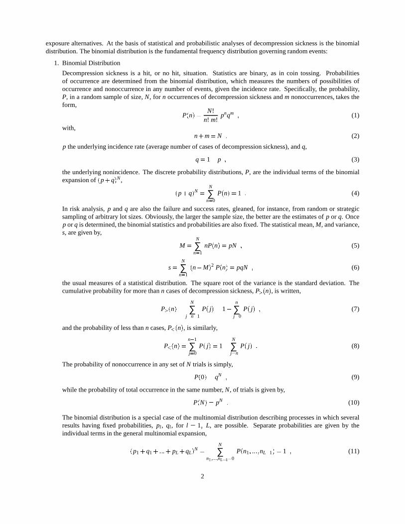
exposure alternatives. At the basis of statistical and probabilistic analyses of decompression sickness is the binomialdistribution. The binomial distribution is the fundamental frequency distribution governing random events:

1. Binomial Distribution

Decompression sickness is a hit, or no hit, situation. Statistics are binary, as in coin tossing. Probabilitiesof occurrence are determined from the binomial distribution, which measures the numbers of possibilities ofoccurrence and nonoccurrence in any number of events, given the incidence rate. Specifically, the probability,P, in a random sample of size, N, for n occurrences of decompression sickness and m nonoccurrences, takes theform,

P(n) =N!

n! m!pnqm ; (1)

with,n+m = N ; (2)

p the underlying incidence rate (average number of cases of decompression sickness), and q,

q = 1 p ; (3)

the underlying nonincidence. The discrete probability distributions, P, are the individual terms of the binomialexpansion of (p+q)N,

(p+q)N =N

∑n=0

P(n) = 1 : (4)

In risk analysis, p and q are also the failure and success rates, gleaned, for instance, from random or strategicsampling of arbitrary lot sizes. Obviously, the larger the sample size, the better are the estimates of p or q. Oncep or q is determined, the binomial statistics and probabilities are also fixed. The statistical mean, M, and variance,s, are given by,

M =N

∑n=1

nP(n) = pN ; (5)

s =N

∑n=1

(nM)2 P(n) = pqN ; (6)

the usual measures of a statistical distribution. The square root of the variance is the standard deviation. Thecumulative probability for more than n cases of decompression sickness, P>(n), is written,

P>(n) =N

∑j=n+1

P( j) = 1n

∑j=0

P( j) ; (7)

and the probability of less than n cases, P<(n), is similarly,

P<(n) =n1

∑j=0

P( j) = 1N

∑j=n

P( j) : (8)

The probability of nonoccurrence in any set of N trials is simply,

P(0) = qN ; (9)

while the probability of total occurrence in the same number, N, of trials is given by,

P(N) = pN : (10)

The binomial distribution is a special case of the multinomial distribution describing processes in which severalresults having fixed probabilities, pl , ql , for l = 1; L, are possible. Separate probabilities are given by theindividual terms in the general multinomial expansion,

(p1 +q1 + :::+ pL +qL)N =

N

∑n1;:::;nL1=0

P(n1; :::;nL1) = 1 ; (11)

2

as in the binomial case. The normal distribution is a special case of the binomial distribution when N is very largeand variables are not necessarily confined to integer values. The Poisson distribution is another special case ofthe binomial distribution when the number of events, N, is also large, but the incidence, p, is small.

2. Normal Distribution

The normal distribution is an analytic approximation to the binomial distribution when N is very large, and n, theobserved value (success or failure rate), is not confined to integer values, but ranges continuously,

∞ n ∞ : (12)

Normal distributions thus apply to continuous observables, while binomial and Poisson distributions apply todiscontinuous observables. Statistical theories of errors are ordinarily based on normal distributions.

For the same mean, M = pN, and variance, s = pqN, the normal distribution, P, written as a continuously varyingfunction of n,

P(n) =1

(2πs)1=2exp [ (nM)2=2s] ; (13)

is a good approximation to the binomial distribution in the range,

1N +1

< p <N

N +1; (14)

and within three standard deviations of the mean,

pN3 (pqN)1=2 n pN +3 (pqN)1=2 : (15)

The distribution is normalized to one over the real infinite interval,Z ∞

∞Pdn = 1 : (16)

The probability that a normally distributed variable, n, is less than or equal to b is,

P<(b) =Z b

∞Pdn ; (17)

while the corresponding probability that n is greater than or equal to b is,

P>(b) =Z ∞

bPdn : (18)

The normal distribution is extremely important in statistical theories of random variables. By the central limittheorem, the distribution of sample means of identically distributed random variables is approximately normal,regardless of the actual distribution of the individual variables.

3. Poisson Distribution

The Poisson distribution is a special case of the binomial distribution when N becomes large, and p is small,and certainly describes all discrete random processes whose probability of occurrence is small and constant. ThePoisson distribution applies substantially to all observations made concerning the incidence of decompressionsickness in diving, that is, p << 1 as the desired norm. The reduction of the binomial distribution to the Poissondistribution follows from limiting forms of terms in the binomial expansion, that is, P(n).

In the limit as N becomes large, and p is much smaller than one, we have,

N!(Nn)!

= Nn ; (19)

qm = (1 p)Nn = exp (pN) ; (20)

3

and therefore the binomial probability reduces to,

P(n) =Nn pn

n!exp (pN) =

Mn

n!exp (M) ; (21)

which is the discrete Poisson distribution. The mean, M, is given as before,

M = pN (22)

and the variance, s, has the same value,s = pN ; (23)

because q is approximately one. The cumulative probabilities, P>(n) and P<(n), are the same as those defined inthe binomial case, a summation over discrete variable, n. It is appropriate to employ the Poisson approximationwhen p :10, and N 10 in trials. Certainly, from a numerical point of view, the Poisson distribution is easierto use than than binomial distribution. Computation of factorials is a lesser task, and bookkeeping is minimal forthe Poisson case.

In addition to the incidence of decompression sickness, the Poisson distribution describes the statistical fluctua-tions in such random processes as the number of cavalry soldiers kicked and killed by horses, the disintegrationof atomic nuclei, the emission of light quanta by excited atoms, and the appearance of cosmic ray bursts. It alsoapplies to most rare diseases.

Probabilistic DecompressionTable 1 lists corresponding binomial decompression probabilities, P(n), for 1% and 10% underlying incidence (99%

and 90% nonincidence), yielding 0, 1, and 2 or more cases of decompression sickness. The underlying incidence, p, isthe (fractional) average of hits.

As the number of trials increases, the probability of 0 or 1 occurrences drops, while the probability of 2 or moreoccurences increases. In the case of 5 dives, the probability might be as low as 5%, while in the case of 50 dives, theprobability could be 39%, both for p = 0:01. Clearly, odds even percentages would require testing beyond 50 casesfor an underlying incidence near 1%. Only by increasing the number of trials for fixed incidences can the probabilitiesbe increased. Turning that around, a rejection procedure for 1 or more cases of decompression sickness at the 10%probability level requires many more than 50 dives. If we are willing to lower the confidence of the acceptance, orrejection, procedure, of course, the number of requisite trials drops. Table 1 also shows that the test practice of acceptingan exposure schedule following 10 trials without incidence of decompression sickness is suspect, merely because therelative probability of nonincidence is high, near 35%.

Questions as to how safe are decompression schedules have almost never been answered satisfactorily. As seen,large numbers of binary events are required to reliably estimate the underlying incidence. One case of decompressionsickness in 30 trials could result from an underlying incidence, p, bounded by .02 and .16 roughly. Tens more of trialsare necessary to shrink those bounds.

Table 1. Probabilities Of Decompression Sickness For Underlying Incidences

P(n) P(n)N (dives) n (hits) p = :01 p = :10

q = :99 q = :905 0 .95 .59

1 .04 .332 or more .01 .08

10 0 .90 .351 .09 .39

2 or more .01 .2620 0 .82 .12

1 .16 .272 or more .02 .61

50 0 .61 .011 .31 .03

2 or more .08 .96

4

Biological processes are highly variable in outcome. Formal correlations with outcome statistics are then generallyrequisite to validate models against data. Often, this correlation is difficult to firmly establish (couple of percent) withfewer than 1,000 trial observations, while ten percent correlations can be obtained with 30 trials, assuming binomialdistributed probabilities. For decompression analysis, this works as a disadvantage, because often the trial space of divesis small. Not discounting the possibly small trial space, a probabilistic approach to the occurrence of decompressionsickness is useful and necessary. One very successful approach, developed and tuned by Weathersby, and others fordecompression sickness in diving, called maximum likelihood, applies theory or models to diving data and adjusts theparameters until theoretical prediction and experimental data are in as close agreement as possible.

Validation procedures require decisions about uncertainty. When a given decompression procedure is repeated withdifferent subjects, or the same subjects on different occasions, the outcome is not constant. The uncertainty about theoccurrence of decompression sickness can be quantified with statistical statements, though, suggesting limits to thevalidation procedure. For instance, after analyzing decompression incidence statistics for a set of procedures, a tabledesigner may report that the procedure will offer an incidence rate below 5%, with 90% confidence in the statement.Alternatively, the table designer can compute the probability of rejecting a procedure using any number of dive trials,with the rejection criteria any arbitrary number of incidences. As the number of trials increases, the probability ofrejecting a procedure increases for fixed incidence criteria. In this way, relatively simple statistical procedures canprovide vital information as to the number of trials necessary to validate a procedure with any level of acceptable risk,or the maximum risk associated with any number of incidences and trials.

One constraint usually facing the statistical table designer is a paucity of data, that is, number of trials of a procedure.Data on hundreds of repetitions of a dive profile are virtually nonexistent, excepting bounce diving perhaps. As seen,some 30-50 trials are requisite to ascertain procedure safety at the 10% level. But 30-50 trials is probably askingtoo much, is too expensive, or generally prohibitive. In that case, the designer may try to employ global statisticalmeasures linked to models in a more complex trial space, rather than a single profile trial space. Integrals of riskparameters, such as bubble number, supersaturation, separated phase, etc., over exposures in time, can be defined asprobability measures for incidence of decompression sickness, and the maximum likelihood method then used to extractappropriate constants:

1. Maximum Likelihood

We can never measure any physical variable exactly, that is, without error. Progressively more elaborate experi-mental or theoretical efforts only reduce the possible error in the determination. In extracting parameter estimatesfrom data sets, it is necessary to also try to minimize the error (or data scatter) in the extraction process. A numberof techniques are available to the analyst, including the well known maximum likelihood approach.

The measure of any random occurrence, p, can be a complicated function of many parameters, x = (xk;k = 1;K),with the only constraint,

0 p(x) 1 ; (24)

for appropriate values of the set, x. The measure of nonoccurence, q, is then by conservation of probability,

q(x) = 1 p(x) ; (25)

over the same range,0 q(x) 1 : (26)

Multivalued functions, p(x), are often constructed, with specific form dictated by theory or observation over manytrials or tests. In decompression applications, the parameters, x, may well be the bubble-nucleation rate, numberof venous gas emboli, degree of supersaturation, amount of pressure reduction, volume of separated gas, ascentrate, or combinations thereof. Parameters may also be integrated in time in any sequence of events, as a globalmeasure, though such measures are more difficult to analyze over arbitrary trial numbers.

The likelihood of any outcome, Φ, of N trials is the product of individual measures of the form,

Φ(n) = pnqm = pn(1 p)m ; (27)

given n cases of decompression sickness and m cases without decompression sickness, and,

n+m = N : (28)

5

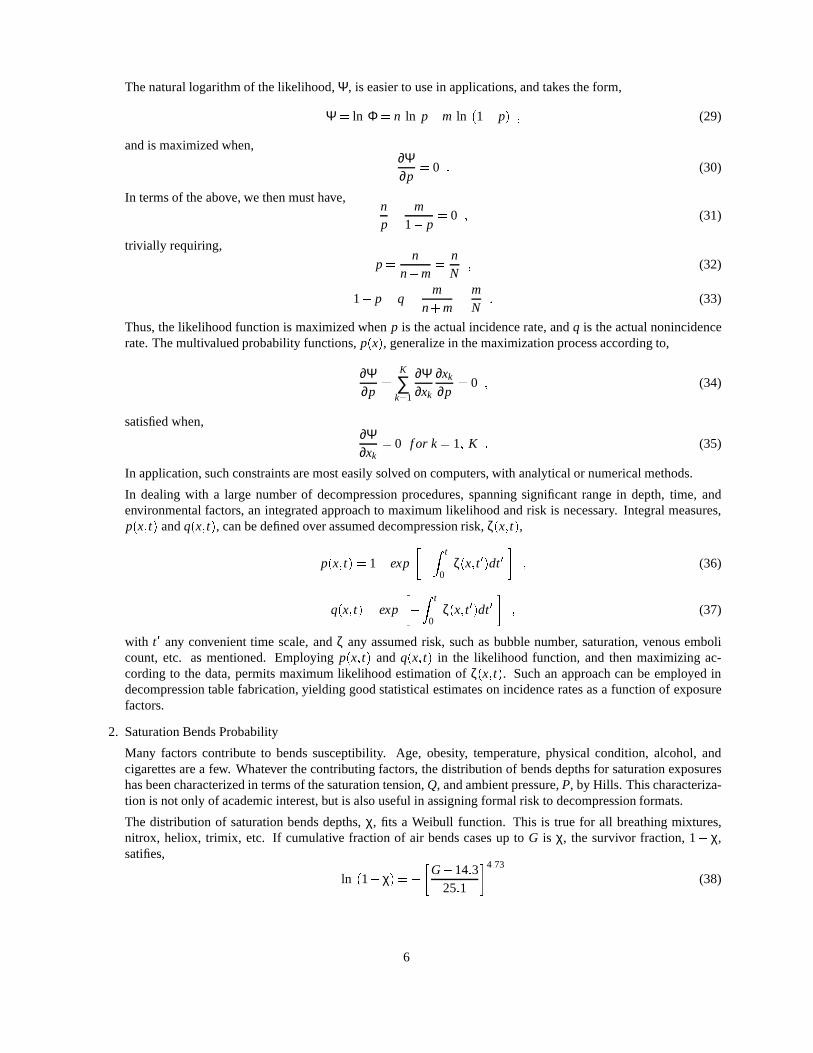
The natural logarithm of the likelihood, Ψ, is easier to use in applications, and takes the form,

Ψ= ln Φ= n ln p+m ln (1 p) ; (29)

and is maximized when,∂Ψ∂p

= 0 : (30)

In terms of the above, we then must have,np

m1 p

= 0 ; (31)

trivially requiring,

p =n

n+m=

nN

; (32)

1 p = q =m

n+m=

mN

: (33)

Thus, the likelihood function is maximized when p is the actual incidence rate, and q is the actual nonincidencerate. The multivalued probability functions, p(x), generalize in the maximization process according to,

∂Ψ∂p

=K

∑k=1

∂Ψ∂xk

∂xk

∂p= 0 ; (34)

satisfied when,∂Ψ∂xk

= 0 f or k = 1; K : (35)

In application, such constraints are most easily solved on computers, with analytical or numerical methods.

In dealing with a large number of decompression procedures, spanning significant range in depth, time, andenvironmental factors, an integrated approach to maximum likelihood and risk is necessary. Integral measures,p(x; t) and q(x; t), can be defined over assumed decompression risk, ζ(x; t),

p(x; t) = 1 exp

Z t

0ζ(x; t 0)dt 0

; (36)

q(x; t) = exp

Z t

0ζ(x; t 0)dt 0

; (37)

with t 0 any convenient time scale, and ζ any assumed risk, such as bubble number, saturation, venous embolicount, etc. as mentioned. Employing p(x; t) and q(x; t) in the likelihood function, and then maximizing ac-cording to the data, permits maximum likelihood estimation of ζ(x; t). Such an approach can be employed indecompression table fabrication, yielding good statistical estimates on incidence rates as a function of exposurefactors.

2. Saturation Bends Probability

Many factors contribute to bends susceptibility. Age, obesity, temperature, physical condition, alcohol, andcigarettes are a few. Whatever the contributing factors, the distribution of bends depths for saturation exposureshas been characterized in terms of the saturation tension, Q, and ambient pressure, P, by Hills. This characteriza-tion is not only of academic interest, but is also useful in assigning formal risk to decompression formats.

The distribution of saturation bends depths, χ, fits a Weibull function. This is true for all breathing mixtures,nitrox, heliox, trimix, etc. If cumulative fraction of air bends cases up to G is χ, the survivor fraction, 1 χ,satifies,

ln (1χ) =

G14:325:1

4:73

(38)

6

for cumulative bends probability, χ, the usual integral over bends risk, ζ, as a function of gradient, G,

χ =

Z G

0ζ(G0)dG0 (39)

with saturation bends gradient, G, measured in f sw,

G = QP (40)

As the gradient grows, the survivor function approaches zero exponentially. The smallest bends gradient is 14.3f sw, which can be contrasted with the average value of 26.5 f sw. The root mean square gradient is 27.5 f sw. At27 f sw, the survivor fraction is 0.96, while 67% of survivors fall in the range, 26:57:6 f sw, with 7.6 f sw thestandard deviation. For gas mixtures other than air, the general form is given by,

ln (1χ) =ε(Pf 20:5)(Pi33:0)

1fi

δ(41)

where fi is the total volume fraction of inert breathing gases, for G = Pf Pi, and with ε, δ constants.

The efficiency of the Weibull distribution in providing a good fit to the saturation data is not surprising. TheWeibull distribution enjoys success in reliability studies involving multiplicities of fault factors. It obviouslyextends to any set of hyperbaric or hypobaric exposure data, using any of the many parameter risk variablesdescribed above.

3. Table And Profile Risks

A global statistical approach to table fabrication consists of following a risk measure, or factor p, throughoutand after sets of exposures, tallying the incidence of DCI, and then applying maximum likelihood to the riskintegral in time, extracting any set of risk constants optimally over all dives in the maximization procedure. Inanalyzing air and helium data, Weathersby assigned risk as the difference between tissue tension and ambientpressure divided by ambient pressure. One tissue was assumed, with time constant ultimately fixed by the data inensuing maximum likelihood analysis. The measure of nonincidence, q, was taken to be the exponential of riskintegrated over all exposure time,

q(κ;τ) = exp

Z ∞

0ζ(κ;τ; t 0)dt 0

; (42)

ζ(κ;τ; t 0) = κp(t 0) pa

pa; (43)

with κ a constant determined in the likelihood maximization, pa ambient pressure, and p(t 0) the instantaneousHaldane tension for tissue with halftime, τ, also determined in the maximization process, corresponding to arbi-trary tissue compartments for the exposure data. Other more complex likelihood functions can also employed, forinstance, the separated phase volume according to the varying permeability and reduced gradient bubble models,

ζ(κ;ξ;τ; t 0) = κΛ(t 0)G(t 0) ; (44)

Λ(t 0) =

1

r(t 0)ξ

; (45)

with Λ the permissible bubble excess, r the bubble radius, G the bubble diffusion gradient (dissolved-free gas),and κ and ξ constants determined in the fit maximization of the data. Another risk possibility is the tissue ratio,

ζ(κ;τ; t 0) = κp(t 0)pa

; (46)

a measure of interest in altitude diving applications.

7

Hundreds of air dives were analyzed using this procedure, permitting construction of decompression scheduleswith 95% and 99% confidence (5% and 1% bends probability). These tables were published by US Navy in-vestigators, and Table 2 tabulates the corresponding nonstop time limits (p = 0:05;0:01), and also includes thestandard US Navy (Workman) limits for comparison. Later re-evaluations of the standard set of nonstop timelimits estimate a probability rate of 1.25% for the limits. In actual usage, the incidence rates are below 0.001%,because users do not dive to the limits generally.

Table 2. Nonstop Time Limits For 1% And 5% DCI Probability

depth nonstop limit nonstop limit nonstop limitd ( f sw) tn (min) tn (min) tn (min)

p = :05 p = :01 US Navy30 240 17040 170 100 20050 120 70 10060 80 40 6070 80 25 5080 60 15 4090 50 10 30

100 50 8 25110 40 5 20120 40 5 15130 30 5 10

Implicit in such formulations of risk tables are the assumptions that a given decompression stress is more likely toproduce symptoms if it is sustained in time, and that large numbers of separate events may culminate in the sameprobability after time integration. Though individual schedule segments may not be replicated enough to offertotal statistical validation, categories of predicted safety can always be grouped within subsets of corroboratingdata. Since the method is general, any model parameter or meaningful index, properly normalized, can be appliedto decompression data, and the full power of statistical methods employed to quantify overall risk. While power-ful, such statistical methods are neither deterministic nor mechanistic, and cannot predict on first principles. Butas a means to table fabrication with quoted risk, such approaches offer attractive pathways for analysis.

For the past 10-15 years, a probabilistic approach to assessing risk in diving has been in vogue. Sometimes thiscan be confusing, or misleading, since definitions or terms, as presented, are often mixed. Also confusing are riskestimates varying by factors of 10 to 1,000, and distributions serving as basis for analysis, also varying in size bythe same factors. So, before continuing with a risk analysis of recreational profiles, a few comments are germane.

Any set of statistical data can be analyzed directly, or sampled in smaller chunks. The smaller sets (samples)may or may not reflect the parent distribution, but if the analyst does his work correctly, samples reflecting theparent distribution can be extracted for study. In the case of dive profiles, risk probabilities extracted from sampleprofiles try to reflect the incidence rate, p, of the parent distribution (N profiles, and p underlying DCI rate). Theincidence rate, p, is the most important metric, followed by the shape of the distribution in total as measured bythe variance, s. For smaller sample of profile size, K < N, we have mean incidences, Q, for sample incidencerate, r,

Q = rK (47)

and variance, v,v = r(1 r)K (48)

By the central limit theorem, the distribution of sample means, Q, is normally distributed about parent (actual)mean, M, with variance, v = s=K. Actually, the distribution of sample means, Q, is normally distributed nomatter what the distribution of samples. This important fact is the basis for error estimation with establishmentof confidence intervals, χ, for r, with estimates denoted, r,

r = rχh s

K

i1=2(49)

8

0 < χ < 1 (50)

The sample binomial probability, B(k), is analogously,

B(k) =K!

k! j!rk(1 r) j (51)

with k+ j = K, for k the number of DCI hits, normalized,

K

∑k=1

B(k) = 1 (52)

and with property, if K ! ∞, then B(k)! 0, when, r << 1.

For example, if 12 cases of DCI are reported in a parent set of 7,896 profiles, then,

N = 7896 (53)

p =12

7896= :0015 (54)

Smaller samples might be used to estimate risk, via sample incidence, r, with samples possibly chosen to reducecomputer processing time, overestimate p for conservancy sake, focus on a smaller subregion of profiles, or anyother reason. Thus, one might nest all 12 DCI incidence profiles in a smaller sample, K = 1;000, so that thesample risk, r = 12=1;000 = 0:012, is larger than p. Usually though the analyst wishes to mirror the parentdistribution in the sample. If the parent is a set of benign, recreational, no decompression, no multiday diveprofiles, and the sample mirrors the parent, then both risks, p and r, are are reasonably true measures of actualrisk associated with recreational diving. If sample distributions chosen are not representative of the class ofdiving performed, risk estimates are not trustworthy. For instance, if a high risk set of mixed gas decompressionprofiles were the background against which recreational dive profiles were compared, all estimates would beskewed and faulty (actually underestimated in relative risk, and overestimated in absolute risk). For this parentset, N is large, p is small, with mean, M = pN = 0:0015 7896 = 12, and the applicable binomial statisticssmoothly transition to Poisson representation, convenient for logarithmic and covariant numerical analysis (on acomputer). Additionally, any parent set may be a large sample of a megaset, so that p is itself an estimate of riskin the megaset.

Turns out that our parent distribution above is just that, a subset of larger megaset, namely, the millions andmillions of recreational dives performed and logged over the past 30 years, or so. The above set of profileswas collected in training and vacation diving scenarios. The set is recreational (no decompression, no multiday,light, benign) and representative, with all the distribution metrics as listed. For reference and perspective, sets ofrecreational profiles collected by others (Gilliam, NAUI, PADI, YMCA, DAN) are similar in context, but largerin size, N, and smaller in incidence rate, p. Data and studies reported by many sources quote, N > 1;000;000,with, p < 0:00001 = 0:001%. Obviously our set has higher rate, p, though still nominally small, but the sameshape. So our estimates will be liberal (overestimate risk).

To perform risk analysis, a risk estimator need be employed. For diving, dissolved gas and phase estimators areuseful. Two, detailed earlier, are used here. First is the dissolved gas supersaturation ratio, historically coupled toHaldane models, φ,

φ= κpλpa

pa(55)

and second, ψ, is the separated phase, invoked by phase models,

ψ = γ

1rξ

G (56)

For simplicity, the asymptotic exposure limit is used in the likelihood integrals for both risk functions,

1 r(κ;λ) = exp

Z ∞

0φ(κ;λ; t)dt

(57)

9

1 r(γ;ξ) = exp

Z ∞

0ψ(γ;ξ; t)dt

(58)

with hitno hit, likelihood function, Ω, of form,

Ω =K

∏k=1

Ωk (59)

Ωk = rδkk (1 rk)

1δk (60)

where, δk = 0 if DCI does not occur in profile, k, or, δk = 1 if DCI does occur in profile, k. To estimate κ, λ, γ,and ξ in maximum likelihood, a modified Levermore-Marquardt algorithm is employed (SNLSE , Common LosAlamos Applied Mathematical Software Library), just a nonlinear least squares data fit to an arbitrary function(minimization of variance over K datapoints here), with L1 error norm. Additionally, using a random numbergenerator for profiles across 1,000 parallel SMP (Origin 2000) processors at LANL, we construct 1,000 subsets,with K = 2;000 and r = 0:006, for separate likelihood regression analysis, averaging κ, λ, γ, and ξ by weightingthe inverse variance.

For recreational diving, both estimators are roughly equivalent, because little dissolved gas has separated intofree phases (bubbles). Analysis shows this true for all cases examined, in that estimated risks for both overlapat the 95% confidence level. The only case where dissolved gas and phase estimators differ (slightly here) iswithin repetitive diving profiles. The dissolved gas estimator cues on gas buildup in the slow tissue compartments(staircasing for repets within an hour or two), while the phase estimator cues on bubble gas diffusion in thefast compartments (dropping rapidly over hour time spans). This holding true within all recreational divingdistributions, we proceed to the risk analysis.

Nonstop limits (NDLs), denoted tn as before, from the US Navy, PADI, and NAUI Tables, and those employed bythe Oceanic decometer provide a set for comparison of relative DCI risk. Listed below in Table 3 are the NDLsand corresponding risks, rn, for the profile, assuming ascent and descent rates of 60 f sw=min (no safety stops).Haldane and RGBM estimates vary little for these cases, and only the phase estimates are included.

Table 3. Risk Estimates For Various NDLs.

USN PADI NAUI Oceanicd ( f sw) tn (min) tn (min) tn (min) tn (min)

35 310 (4.3%) 205 (2.0%) 181 (1.3%)40 200 (3.1%) 140 (1.5%) 130 (1.4%) 137 (1.5%)50 100 (2.1%) 80 (1.1%) 80 (1.1%) 80 (1.1%)60 60 (1.7%) 55 (1.4%) 55 (1.4%) 57 (1.5%)70 50 (2.0%) 40 (1.2%) 45 (1.3%) 40 (1.2%)80 40 (2.1%) 30 (1.3%) 35 (1.5%) 30 (1.3%)90 30 (2.1%) 25 (1.5%) 25 (1.5%) 24 (1.4%)

100 25 (2.1%) 20 (1.3%) 22 (1.4%) 19 (1.2%)110 20 (2.2%) 13 (1.1%) 15 (1.2%) 16 (1.3%)120 15 (2.0%) 13 (1.3%) 12 (1.2%) 13 (1.3%)130 10 (1.7%) 10 (1.7%) 8 (1.3%) 10 (1.7%)

Risks are internally consistent across NDLs at each depth, and agree with the US Navy assessments in Table 2.Greatest underlying and binomial risks occur in the USN shallow exposures. The PADI, NAUI, and Oceanic risksare all less than 2% for this set, thus binomial risks for single DCI incidence are less than 0.02%. PADI and NAUIhave reported that field risks (p) across all exposures are less than 0.001%, so considering their enviable trackrecord of diving safety, our estimates are liberal. Oceanic risk estimates track as the PADI and NAUI risks, again,very safely.

Next, the analysis is extended to profiles with varying ascent and descent rates, safety stops, and repetitive se-quence. Table 4 lists nominal profiles (recreational) for various depths, exposure and travel times, and safety

10

stops at 5 msw. DCI estimates, r, are tabulated for both dissolved gas supersaturation ratio and bubble numebrexcess risk functions.

Table 4. Dissolved And Separated Phase Risk Estimates For Nominal Profiles.

profile descent rate ascent rate safety stop r r(depth=min) (msw=min) (msw=min) (depth=min) RGBM ZHL

14 msw/38 min 18 9 5 msw/3 min .0034 .006219 msw/38 min 18 9 5 msw/3 min .0095 .011037 msw/17 min 18 9 5 msw/3 min .0165 .0151

18 msw/31 min 18 9 5 msw/3 min .0063 .007218 9 .0088 .008418 18 .0101 .013518 18 5 msw/3 min .0069 .0084

17 msw/32 min 18 9 5 msw/3 minSI 176 min

13 msw/37 min 18 9 5 msw/3 minSI 174 min

23 msw/17 min 18 18 5 msw/3 min .0127 .0232

The ZHL (Buhlmann) NDLs and staging regimens are widespread across decompression meters presently, andare good representation for Haldane risk analysis. The RGBM is newer and more modern (and more physicallycorrect), and is coming online in decometers and associated software. For recreational exposures, the RGBMcollapses to a Haldane dissolved gas algorithm. This is reflected in the risk estimates above, where estimates forboth models differ little.

Simple comments hold for the analyzed profile risks. The maximum relative risk is 0.0232 for the 3 dive repet-itive sequence according to the Haldane dissolved risk estimator. This translates to .2% binomial risk, which iscomparable to the maximum NDL risk for the PADI, NAUI, and Oceanic NDLs. Again, this type of dive profileis common, practiced daily on liveaboards, and benign. According to Gilliam, the absolute incidence rate for thistype of diving is less than 0.02%. Again, our figures overestimate risk.

Effects of slower ascent rates and safety stops are noticeable at the 0.25% to 0.5% level in relative surfacingrisk. Safety stops at 5 m for 3 min lower relative risk an average of 0.3%, while reducing the ascent rate from 18msw=min to 9 msw=min reduces relative risk an average of 0.35%.

Staging, NDLs, and other contraints imposed by decometer algorithms are entirely consistent with acceptableand safe recreational diving protocols. The estimated absolute risk associated across all ZHL NDLs and diverstaging regimens analyzed herein is less than .232%, and is probably much less in actual practice. That is, we usep = 0:006, and much evidence suggests p < 0:0001, some ten times safer.

Model ValidationValidation procedures for schedules and tables can be quantified by a set of procedures based on statistical decom-

pression analysis:

1. select or construct a measure of decompression risk, or a probabilistic model;

2. evaluate as many dives as possible, and especially those dives similar in exposure time, depth, and environmentalfactors;

3. conduct limited testing if no data is available;

4. apply the model to the data using maximum likelihood;

11

5. construct appropriate schedules or tables using whatever incidence of decompression sickness is acceptable;

6. release and then collect profile statistics for final validation and tuning.

Questions of what risk is acceptable to the diver vary. Sport and research divers would probably opt for very smallrisk (0.01% or less), while military and commercial divers might live with higher risk (1%), considering the nearness ofmedical attention in general. Many factors influence these two populations, but fitness and acclimatization levels wouldprobably differ considerably across them. While such factors are difficult to fold into any table exercise or analysis, thesimple fact that human subjects in dive experiments exhibit higher incidences during testing phases certainly helps tolower the actual incidence rate in the field, noted by Bennett and Lanphier.

Certainly there is considerable latitude in model assumptions, and many plausible variants on a theme. Manymodels are correlated with diving exposure data, using maximum likelihood to fit parameters or other valid statisticalapproaches, but not all. Most have been applied to profiles outside of tested ranges, when testing has been performed,in an obvious extrapolation mode. Sometimes the extrapolations are valid, other times not.

REDUCED GRADIENT BUBBLE MODEL

Bubble DynamicsCrucial to all bubble models are the concepts of critical radii and bubble growth. The critical radius, r0, at fixed

pressure, P0, represents the cutoff for growth upon decompression to lesser pressure. Nuclei larger than r0 will all growupon decompression. Additionally, following an initial compression, ∆P = PP0, a smaller class of micronuclei ofcritical radius, r, can be excited into growth with decompression. If r0 is the critical radius at P0, then, the smallerfamily, r, excited by decompression from greater P, obeys for all pressure P and temperature T ,

r = α +β

TP

1=3

+κ

TP

2=3

(61)

with α, β, and κ equation-of-state (EOS) skin constants, P the absolute pressure in f sw, and T the absolute temperaturein Ko. Table 5 lists critical radii, r, excited by sea level compressions, P0 = 33 f sw, for r0 = 1:36 µm, and T0 = 293 Ko.Entries are the equilibrium critical radii at pressure, P.

Table 5. Micronuclei Excitation Radii

pressure excitation radius pressure excitation radiusP ( f sw) r (µm) P ( f sw) r (µm)

13 2.10 153 1.1833 1.36 173 1.1353 1.34 193 1.0873 1.32 213 1.0293 1.28 233 .96

113 1.24 253 .90133 1.20 273 .80

The permissible gradient, G, is written for each compartment, τ, using the standard formalism,

G = G0 +∆Gd (62)

at depth d = P33 f sw. A nonstop bounce exposure, followed by direct return to the surface, thus allows G0 for thatcompartment. One set G0 and ∆G are tabulated in Table 6, with ∆G suggested by Buhlmann. The minimum excitation,Gmin, initially probing r, and taking into account regeneration of nuclei over time scales τr, is ( f sw),

Gmin =2 γ (γcγ)

γc r(t)=

11:01r(t)

(63)

12

with,r(t) = r+(r0 r) [1 exp (λrt)] (64)

γ, γc film, surfactant surface tensions, that is, γ= 17:9 dyne=cm, γc = 257 dyne=cm, and λr the inverse of the regenerationtime for stabilized gas micronuclei (many days). Prolonged exposure leads to saturation, and the largest permissiblegradient, Gsat , takes the form ( f sw), in all compartments,

Gsat =58:6

r49:9 = :372 P+11:01: (65)

On the other hand, Gmin is the excitation threshold, the amount by which the surrounding tension must exceeed internalbubble pressure to just support growth.

Although the actual size distribution of gas nuclei in humans is unknown, experiments in vitro suggest that a decay-ing exponential is reasonable,

n = N exp (βr) (66)

with β a constant, and N a convenient normalization factor across the distribution. For small values of the argument, βr,

exp (βr) = 1βr (67)

as a nice simplification. For a stabilized distribution, n0, accommodated by the body at fixed pressure, P0, the excessnumber of nuclei, Λ, excited by compression-decompression from new pressure, P, is,

Λ = n0n = Nβr0

1

rr0

: (68)

For large compressions-decompressions, Λ is large, while for small compressions-decompressions, Λ is small. When Λis folded over the gradient, G, in time, the product serves as a critical volume indicator and can be used as a limit pointin the following way.

Phase Volume LimitsThe rate at which gas inflates in tissue depends upon both the excess bubble number, Λ, and the gradient, G. The

critical volume hypothesis requires that the integral of the product of the two must always remain less than some limitpoint, α V , with α a proportionality constant, Z ∞

0ΛGdt = αV (69)

for V the limiting gas volume. Assuming that gradients are constant during decompression, td , while decaying expo-nentially to zero afterwards, and taking the limiting condition of the equal sign, yields simply for a bounce dive, with λthe tissue constant,

ΛG (td +λ1) = αV: (70)

In terms of earlier parameters, one more constant, δ, closes the set, defined by,

δ=γc α V

γ β r0 N(71)

so that, 1

rr0

G (td +λ1) = δ

γγc

(72)

The five parameters, γ, γc, δ, λr, r0, are five of the six fundamental constants in the varying permeability model. Theremaining parameter, λm, interpolating bounce and saturation exposures, represents the inverse time contant modulatingmultidiving. Bubble growth experiments suggest that λ1

m is in the neighborhood of an hour. Discussion of λm follows.The depth at which a compartment controls an exposure, and the excitation radius as a function of halftime, τ, in

the range, 12 d 220 f sw, satisfy,rr0

= :9 :43 exp (ζτ) (73)

13

with ζ = :0559 min1. The regeneration constant, λr, is on the order of inverse hours, that is, λr = :1733 hours1.Characteristic halftimes, τr and τm, take the values τr = 4 hrs and τm = 30 min. For large τ, r is close to r0, while forsmall τ, r is on the order of .5 r0. At sea level, r0 = 1:36 microns as discussed.

The phase (limit) integral for multiexposures is written,

J

∑j=1

ΛG td j +

Z t j

0ΛGdt

α V (74)

with the index j denoting each dive segment, up to a total of J, and t j the surface interval after the jth segment. For theinequality to hold, that is, for the sum of all growth rate terms to total less than αV , obviously each term must be lessthe α V . Assuming that tJ ! ∞, gives,

J1

∑j=1

ΛG [td j +λ1

λ1exp (λt j)]+ΛG (tdJ +λ1) α V: (75)

Defining G j,ΛG j (td j +λ1) = ΛG (td j +λ1)ΛG λ1exp (λt j1) (76)

for j = 2 to J, and,ΛG1 = ΛG (77)

for j = 1, it follows thatJ

∑j=1

Λ G j (td j +λ1) α V (78)

with the important property,G j G: (79)

This implies we employ reduced gradients extracted from bounce gradients by writing,

G j = ξ j G (80)

with ξ j a multidiving fraction requisitely satisfying,

0 ξ j 1 (81)

so that, as needed,ΛG j ΛG: (82)

The fractions, ξ, applied to G always reduce them. As time and repetitive frequency increase, the body’s ability toeliminate excess bubbles and nuclei decreases, so that we restrict the permissible bubble excess in time,

Λ(tcumj1) = Nβr0

"1

r(tcumj1)

r0

#= Λ exp (λrt

cumj1) (83)

tcumj1 =

j1

∑i=1

ti (84)

with tcumj1 cumulative dive time. A reduction factor, ηreg

j , accounting for creation of new micronuclei is taken to be theratio of present excess over initial excess, written,

ηregj =

Λ(tcumj1)

Λ= exp (λrt

cumj1) (85)

For reverse profile diving, the gradient is restricted by the ratio (minimum value) of the bubble excess on the presentsegment to the bubble excess at the deepest point over segments. The gradient reduction, ηexc

j , is then,

ηexcj =

(Λ)max

(Λ) j=

(rd)max

(rd) j(86)

14

with rd the product of the appropriate excitation radius and depth. Because bubble elimination periods are shortenedover repetitive dives, compared to intervals for bounce dives, the gradient reduction, ηrep

j , is proportional to the differ-ence between maximum and actual surface bubble inflation rate, that is,

ηrepj = 1

1

Gmin

G

exp (λmt j1) (87)

with t j1 consecutive surface interval time, λ1m on the order of an hour, and Gmin the smallest G0 in Table 6.

Finally, for multidiving, the gradient reduction factor, ξ, is defined bt the product of the three η,

ξ j = ηexcj ηrep

j ηregj =

(Λ)max

(Λ) j

1

1

Gmin

G

exp (λmt j1)

exp (λrt

cumj1) (88)

with t j1 consecutive dive time, and tcumj1 cumulative dive time, as noted. Since bubble numbers increase with depth,

reduction in permissible gradient is commensurate. Multiday diving is mostly impacted by λr, while repetitive divingmostly by λm. Obviously, the critical tension, M, takes the form,

M = ξ(G0 +∆Gd)+P: (89)

Table 6 tabulates a (sample) set of RGBM critical gradients, G0 and ∆G.

Table 6. Critical Phase Volume Gradients

halftime threshold depth surface gradient gradient changeτ (min) δ ( f sw) G0 ( f sw) ∆G

2 190 151.0 .5185 135 95.0 .515

10 95 67.0 .51120 65 49.0 .50640 40 36.0 .46880 30 27.0 .417

120 28 24.0 .379240 16 23.0 .329480 12 22.0 .312

Parameter RangesOver a range of depths, exposures, repetitive frequency, and gas mixtures, the parameter sets of the RGBM are

roughly limited as follows,0:64 µm r0 2:84 µm

15 dyne=cm γ 65 dync=cm

160 dyne=cm γc 290 dyne=cm

6500 f sw min δ 8300 f sw min

2 hrs τr 6 hr

20 min τm 140 min

with nonstop, altitude, decompression, saturation, nitrox, heliox, trimix, and repetitive exposures down to 550 f sw in-cluded in the range analysis. Values of the these parameters are also consistent with biophysical estimates, experimentaldata, and theoretical models across aquaeous and lipid substances. Given our present state of knowledge, nothing isincompatible in the ranges listed.

15

RGBM/ZHL (Critical Parameter) SYNTHESIS

Profile And Parameter MatchingThe following is specific to the ZHL implementation of the RGBM across critical parameters and nonstop time

limits of the RGBM/ZHL algorithm. Extensive computer fitting of profiles and recalibration of parameters to maintainthe RGBM within the ZHL limits is requisite here. ABYSS has implemented this synthesis into Internet diveware.

1. Critical Parameters (a, b)

Haldane approaches use a simple dissolved gas (tissue) transfer equation, and a set of critical parameters todictate diver staging through the gas transfer equation. In the Workman approach, the critical parameters arecalled M values, while in the Buhlmann formulation they are called a and b. They are equivalent sets, slightlydifferent in representation but not content, First consider the transfer equation for air.

Tissue tensions (nitrogen partial pressures), p, for ambient nitrogen partial pressure, pa, and initial tissue tension,pi, evolve in time, t, in standard fashion in compartment, τ, according to,

p pa = (p pa) exp (λt) (90)

for,

λ =:693

τ(91)

with τ tissue halftime, and, for air,pa = :79 P (92)

and with ambient pressure, P, given as a function of depth, d, in units of f sw,

P = d +P0 (93)

Staging is controlled in the Buhlmann ZHL algorithm through sets of tissue parameters, a and b, listed below inTable 6 for 14 tissues, τ, through the minimum permissible (tolerable) ambient pressure, Pmin, by,

Pmin = (pa)b (94)

across all tissue compartments, τ, with the largest Pmin limiting the allowable ambient pressure, Pmin. Recall that,

1 bar = 1:013 atm ; 1 atm = 33 f sw

as conversion metric between bar and f sw in pressure calculations. Linear extrapolations across tissue compart-ments are often used for different sets of halftimes and critical parameters, a and b.

Table 7. Nitrogen ZHL Critical Parameters (a, b)

halftime critical intercept critical slopeτ (min) a (bar) b

5.0 1.198 .54210.0 .939 .68720.0 .731 .79340.0 .496 .86865.0 .425 .88290.0 .395 .900

120.0 .372 .912150.0 .350 .922180.0 .334 .929220.0 .318 .939280.0 .295 .944350.0 .272 .953450.0 .255 .958635.0 .236 .966

16

In terms of critical tensions, M, according to the USN, the relationship linking the two sets is simply,

M =Pb+a = ∆M P+M0 (95)

so that,

∆M =1b

(96)

M0 = a (97)

in units of bar, though the usual representation for M is f sw. The above set, a and b, hold generally for nitrox,and, to low order, for heliox (and trimix too). Tuned modifications for heliox and trimix are also tabulated below.

Corresponding nonstop time limits, tn, are listed in Table 8, and the nonstop limits follow the Hempleman squareroot law, roughly,

dt1=2n = 475 f sw min1=2 (98)

in a least squares fit. The square root law also follows directly from the form of the bulk diffusion transferequation, but not from any Haldane assumptions nor limiting forms of the tissue equation.

Table 8. Air ZHL Nonstop Time Limits

depth timed f sw tn (min)

30 29040 13050 7560 5470 3880 2690 22

100 20110 17120 15130 11140 9150 8160 7170 6180 5190 4200 3

2. Likelihood Profile And Model Analysis

Over ranges of depths, tissue halftimes, and critical parameters of the ZHL algorithm, approximately 2,300dive profiles were simulated using both the RGBM (Part 2) and Haldane ZHL algorithms. To correlate the twoas closely as possible to the predictions of the RGBM across these profiles, maximum likelihood analysis isused, that is, extracting the temporal features of three bubble parameters mating the RGBM and ZHL algorithmsextending critical parameters of the ZHL Haldane model to more complete bubble dynamical framework andphysical basis. These factors, f , are described next, with their linkages to a and b, and are the well knownreduction f actors of the RGBM.

3. Multidiving Fractions

According to the RGBM fits across the ZHL profiles (2,300), a correlation can be established through multidivingreduction factors, f , such that for any set of nonstop gradients, G,

G = MP (99)

17

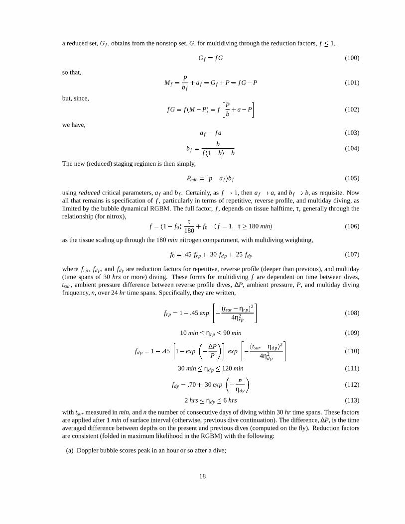
a reduced set, G f , obtains from the nonstop set, G, for multidiving through the reduction factors, f 1,

G f = f G (100)

so that,

Mf =Pb f

+a f = G f +P = f G+P (101)

but, since,

f G = f (MP) = f

Pb+aP

(102)

we have,a f = f a (103)

b f =b

f (1b)+b(104)

The new (reduced) staging regimen is then simply,

Pmin = (pa f )b f (105)

using reduced critical parameters, a f and b f . Certainly, as f ! 1, then a f ! a, and b f ! b, as requisite. Nowall that remains is specification of f , particularly in terms of repetitive, reverse profile, and multiday diving, aslimited by the bubble dynamical RGBM. The full factor, f , depends on tissue halftime, τ, generally through therelationship (for nitrox),

f = (1 f0)τ

180+ f0 ( f = 1; τ 180 min) (106)

as the tissue scaling up through the 180 min nitrogen compartment, with multdiving weighting,

f0 = :45 frp + :30 fd p + :25 fdy (107)

where frp, fd p, and fdy are reduction factors for repetitive, reverse profile (deeper than previous), and multiday(time spans of 30 hrs or more) diving. These forms for multidiving f are dependent on time between dives,tsur, ambient pressure difference between reverse profile dives, ∆P, ambient pressure, P, and multiday divingfrequency, n, over 24 hr time spans. Specifically, they are written,

frp = 1 :45 exp

"(tsurηrp)

2

4η2rp

#(108)

10 min ηrp 90 min (109)

fd p = 1 :45

1 exp

∆PP

exp

"(tsurηd p)

2

4η2d p

#(110)

30 min ηd p 120 min (111)

fdy = :70+ :30 exp

nηdy

(112)

2 hrs ηdy 6 hrs (113)

with tsur measured in min, and n the number of consecutive days of diving within 30 hr time spans. These factorsare applied after 1 min of surface interval (otherwise, previous dive continuation). The difference, ∆P, is the timeaveraged difference between depths on the present and previous dives (computed on the fly). Reduction factorsare consistent (folded in maximum likelihood in the RGBM) with the following:

(a) Doppler bubble scores peak in an hour or so after a dive;

18

(b) reverse profiles with depth increments beyond 50 f sw incur increasing DCI risk, somewhere between 5%and 8% in the depth increment range of 40 f sw - 120 f sw;

(c) Doppler bubble counts drop tenfold when ascent rates drop from 60 f sw=min to 30 f sw=min;

(d) multiday diving risks increase by factors of 2 -3 (though still small) over risk associated with a single dive.

4. Nitrox

The standard set, a, b, and τ, given in Table 7 hold across nitrox exposures, and the tissue equation remainsthe same. The obvious change for a nitrox mixture with nitrogen fraction, fN2 , occurs in the nitrogen ambientpressure, paN2 , at depth, d, in analogy with the air case,

paN2 = fN2 P = fN2 (d +P0) (114)

with P ambient pressure ( f sw). All else is unchanged. The case, fN2 = .79, obviously represents an air mixture.

5. Heliox

The standard set, a, b, and τ is modified for helium mixtures, with basic change in the set of halftimes, τ, used forthe set, a and b, To lowest orderset, a and b for helium are the same as those for nitrogen, though we will list themodifications in Table 9 below. Halftimes for helium are approximately 2.65 times faster than those for nitrogen,by Graham’s law (molecular diffusion rates scale inversely with square root of atomic masses). That is,

τHe =τN2

2:65(115)

because helium is approximately 7 times lighter than nitrogen, and diffusion rates scale with square root of theratio of atomic masses. The tissue equation is the same as the nitrox tissue equation, but with helium constants,λ, defined by the helium tissue halftimes. Denoting the helium fraction, fHe, the helium ambient pressure, paHe,is given by,

paHe = fHe P = fHe (d +P0) (116)

as with nitrox. Multidiving fractions are the same, but the tissue scaling is different across the helium set,

f = (1 f0)τ

67:8+ f0 ( f = 1; τ 67:8 min) (117)

and all else is the same.

Table 9. Helium ZHL Critical Parameters (a, b)

halftime critical intercept critical slopeτ (min) a (bar) b

1.8 1.653 .4613.8 1.295 .6047.6 1.008 .729

15.0 .759 .81624.5 .672 .83733.9 .636 .86445.2 .598 .87656.6 .562 .88567.8 .541 .89283.0 .526 .901

105.5 .519 .906132.0 .516 .914169.7 .510 .919239.6 .495 .927

19

6. Trimix

For trimix, both helium and nitrogen must be tracked with tissue equations, and appropriate average of heliumand nitrogen critical parameters used for staging. Thus, denoting nitrogen and helium fractions, fN2 , and fHe,ambient nitrogen and helium pressures, paN2 and paHe, take the form,

paN2 = fN2 P = fN2 (d +P0) (118)

paHe = fHe P = fHe (d +P0) (119)

Tissue halftimes are mapped exactly as listed in Tables 5 and 6, and used appropriately for nitrogen and heliumtissue equations. Additionally,

fO2 + fN2 + fHe = 1 (120)

and certainly in Tables 5 and 6, one has the mapping,

τHe =τN2

2:65(121)

Then, total tension, Π, is the sum of nitrogen and helium components,

Π = (paN2 + paHe)+(piN2 paN2) exp (λN2t)+(piHe paHe) exp (λHet) (122)

with λN2 and λHe decay constant for the nitrogen and helium halftimes in Tables 5 and 6. Critical parameters fortrimix, α f and β f , are just weighted averages of critical parameters, aN2 , bN2 , aHe bHe, from Tables 5 and 6, thatis, generalizing to the reduced set, a f and b f ,

α f =fN2 a f N2 + fHea f He

fN2 + fHe(123)

β f =fN2 b f N2 + fHeb f He

fN2 + fHe(124)

The staging regimen for trimix is,Pmin = (Πα f )β f (125)

as before. The corresponding critical tension, Mf , generalizes to,

Mf =Pβ f

+α f (126)

Synthesis SummaryOverall, the RGBM algorithm is conservative with safety imparted to the Haldane ZHL model through multidiving

f factors. Estimated DCI incidence rate from likelihood analysis is 0.001% at the 95% confidence level for the overallRGBM. Table and meter implementations with consistent coding should reflect this estimated risk. Similar estimatesand comments apply to the ZHL mixed gas synthesis.

PHASE (RGBM) AND HALDANE CONTRASTS

RGBM For The LaymanThe following discourse charts in layman terms the differences between phase models, such as the full RGBM and

RGBM/ZHL, and dissolved gas models, such as the ZHL of Buhlmann.

Empirical PracticesUtilitarian procedures, entirely consistent with phase mechanics and bubble dissolution time scales, have been

developed under duress, and with trauma, by Australian pearl divers and Hawaiian diving fishermen, for both deepand repetitive diving with possible in-water recompression for hits. While the science behind such procedures was

20

not initially clear, the operational effectiveness was always noteworthy and could not be discounted easily. Later, therationale, essentially recounted in the foregoing, became clearer.

Pearling fleets, operating in the deep tidal waters off northern Australia, employed Okinawan divers who regularlyjourneyed to depths of 300 f sw for as long as one hour, two times a day, six days per week, and ten months out of theyear. Driven by economics, and not science, these divers developed optimized decompression schedules empirically.As reported by Le Messurier and Hills, deeper decompression stops, but shorter decompression times than required byHaldane theory, were characteristics of their profiles. Such protocols are entirely consistent with minimizing bubblegrowth and the excitation of nuclei through the application of increased pressure, as are shallow safety stops andslow ascent rates. With higher incidence of surface decompression sickness, as might be expected, the Australiansdevised a simple, but very effective, in-water recompression procedure. The stricken diver is taken back down to30 f sw on oxygen for roughly 30 minutes in mild cases, or 60 minutes in severe cases. Increased pressures help toconstrict bubbles, while breathing pure oxygen maximizes inert gas washout (elimination). Recompression time scalesare consistent with bubble dissolution experiments.

Similar schedules and procedures have evolved in Hawaii, among diving fishermen, according to Farm and Hayashi.Harvesting the oceans for food and profit, Hawaiian divers make beween 8 and 12 dives a day to depths beyond 350f sw. Profit incentives induce divers to take risks relative to bottom time in conventional tables. Three repetitive divesare usually necessary to net a school of fish. Consistent with bubble and nucleation theory, these divers make theirdeep dive first, followed by shallower excursions. A typical series might start with a dive to 220 f sw, followed by 2dives to 120 f sw, and culminate in 3 or 4 more excursions to less than 60 f sw. Often, little or no surface intervalsare clocked between dives. Such types of profiles literally clobber conventional tables, but, with proper reckoning ofbubble and phase mechanics, acquire some credibility. With ascending profiles and suitable application of pressure, gasseed excitation and any bubble growth are constrained within the body’s capacity to eliminate free and dissolved gasphases. In a broad sense, the final shallow dives have been tagged as prolonged safety stops, and the effectiveness ofthese procedures has been substantiated in vivo (dogs) by Kunkle and Beckman. In-water recompression procedures,similar to the Australian regimens, complement Hawaiian diving practices for all the same reasons.

While the above practices developed by trial-and-error, albeit with seeming principle, venous gas emboli measure-ments, performed off Catalina by Pilmanis on divers making shallow safety stops, fall into the more scienti f ic categoryperhaps. Contrasting bubble counts following bounce exposures near 100 f sw, with and without zonal stops in the10-20 f sw range, marked reductions (factors of 4 to 5) in venous gas emboli were noted when stops were made. If, assome suggest, venous gas emboli in bounce diving correlate with bubbles in sites such as tendons and ligaments, thensafety stops probably minimize bubble growth in such extravascular locations. In these tests, the sample population wassmall, so additional validation and testing is warranted.

Only a handful of hard and fast conclusions about DCI can be drawn from present knowledge. So elementary as tobe innocuous, they are stated:

1. bubble inception or phase separation is the primary event triggering simple decompression sickness;

2. prevention of decompression sickness amounts to prevention (as a limit) of bubble inception or phase separation;

3. gradual pressure reductions prevent bubble formation.

As known by many, after the above attempts at concensus usually diverge. Modelers and table designers must thensupply, or assume, gas exchange models, trigger points, and safe diving protocols which prevent or, at least, minimizephase inception and bubble growth.

Present notions of nucleation and cavitation suggest that decompression phase separation is random, yet highlyprobable, in body tissue. Once established, a gaseous phase will further grow by acquiring gas from adjacent saturatedtissue, according to the strength of the free-dissolved gradient. Although exchange mechanisms are better understood,nucleation and stabilization mechanisms remain less so, and calculationally elusive. Stochastic Monte Carlo bubbletracking methods are powerful, but only in supercomputer environments, due to the large number of events required formeaningful statistics over simulation time spans. Exchange models for entrained bubbles and coalescence dynamics aresimilarly complicated. In all cases, more knowledge about gas micronuclei and size distributions, tissue sites, thermo-dynamics properties, stabilization, and excitation mechanisms is necessary before computing power can be leveragedto decompression modeling.

21

But even with a paucity of knowledge, many feel that empirical practices and recent studies on bubbles and nucleished considerable light on growth and elimination processes, and time scales. Their consistency with underlying phys-ical principles suggest directions for table and meter modeling, beyond parameter fitting and extrapolation techniques.Recovering dissolved gas algorithms for short exposure times, phase models link to bubble mechanics and critical vol-ume trigger points. Bubble and phase models support the efficacy of recently suggested safe diving practices, by simplevirtue of dual phase mechanics:

1. reduced nonstop time limits;

2. safety stops (or shallow swimming ascents) in the 10-20 f sw zone, 1-2 min for dives in the 40-90 f sw range, 2-3min for dives in the 90-240 f sw range;

3. ascent rates not exceeding 30 f sw=min;

4. restricted repetitive exposures, particularly beyond 100 f sw, based on reduction in permissible bubble excessover time;

5. restricted spike (shallow-to-deep) exposures based on excitation of additional micronuclei;

6. restricted multiday activity based on regeneration of micronuclei over longer time scales;

7. smooth coalescence of bounce and saturation limit points, consistent with bubble experiments;

8. consistent model treatment of altitude diving;

Bubble models also tend to be consistent with the utilitarian measures observed for diving practice. Conservatismmay be downplayed in some meter implementations, yet medical authorities are becoming increasingly concernedabout long term effects of breathing pressurized gases. On firmer principles, bubble models tend to corroborate safetymeasures in multidiving, and thus one might reasonably expect to witness their further development. Said another way,bubble models have the right physical signatures for diving application.

Phase Versus Haldane ProfilesSuunto, HydroSpace, and Abysmal Diving have released products incorporating a modern phase algorithm, the

above Reduced Gradient Bubble Model (RGBM), for diving. An iterative approach to staging diver ascents, the RGBMemploys separated phase volumes as limit points, instead of the usual Haldane (maximum) critical tensions across tissuecompartments. The model is inclusive (altitude, repetitive, mixed gas, decompression, saturation, nonstop exposures),treating both dissolved and free gas phase buildup and elimination. NAUI Technical Diving employed the RGBM toschedule nonstop and decompression training protocols on trimix, heliox, and nitrox while also testing gas switchingalternatives for deep exposures. The RGBM has its roots in the earlier work of the Tiny Bubble Group at the Universityof Hawaii, drawing upon and extending the so-called Varying Permeability Model (VPM) to multidiving, altitude, andmixed gas applications. While certainly not radical, the RGBM is both different and new on the diving scene. Andnot unexpectedly, the RGBM recovers the Haldane approach to decompression modeling in the limit of relatively safe(tolerably little) separated phase, with tolerably little a qualitative statement here.

The Suunto VYPER/COBRA/STINGER are RGBM-based decometers for recreational diving (plus nitrox), whileRGBM/ABYSS is a licensed Abysmal Diving software product. The HydroSpace Engineering EXPLORER is a fullmixed gas (nitrox, heliox, trimix) decompression meter for recreational and technical diving, and employs the RGBM.On the Internet, the sites htt p : ==www:suunto: f i=diving:index:html and htt p : ==www:abysmal:com=index:html can bevisited for information and description. All are first-time-ever commercial products with realistic implementation of adiving phase algorithm across a wide spectrum of exposure extremes. And all accommodate user knobs for additionalconservatism. Expect RGBM coded software to surface in other dive computers. And expect other vendors to releaseRGBM based diving software for mixed gases.

Here, our intent is to (just) look at the underpinnings of both meter and diveware implementations of the RGBMalgorithm, one with extended range of applicability based on simple dual phase principles. Haldane approaches havedominated decompression algorithms for a very long time, and the RGBM has been long in coming on the commercialscene. With recent technical diving interest in deep stop modeling, and concerns with repetitive diving in the recreationalcommunity, phase modeling is timely and pertinent. And, of course, since the RGBM extends the VPM, much of thefollowing applies to the VPM directly.

22

Recent years have witnessed many changes and modifications to diving protocols and table procedures, such asshorter nonstop time limits, slower ascent rates, discretionary safety stops, ascending repetitive profiles, multileveltechniques, both faster and slower controlling repetitive tissues, smaller critical tensions (M-values), longer flying-after-diving surface intervals, and others. Stimulated by observation, Doppler technology, decompression meter development,theory, statistics, or safer diving concensus, these modifications affect a gamut of activity, spanning bounce to multidaydiving. Of these changes, conservative nonstop time limits, no decompression safety stops, and slower ascent rates(around 30 f sw=min) are in vogue, and have been incorporated into many tables and meters. As you might expect,recent developments support them on operational, experimental, and theoretical grounds.

But there is certainly more to the story as far as table and meter implementations. To encompass such far reaching(and often diverse) changes in a unified framework requires more than the simple Haldane models we presently relyupon in 99% of our tables and dive computers. To model gas transfer dynamics, modelers and table designers needaddress both free and dissolved gas phases, their interplay, and their impact on diving protocols. Biophysical modelsof inert gas transport and bubble formation all try to prevent decompression sickness. Developed over years of divingapplication, they differ on a number of basic issues, still mostly unresolved today:

1. the rate limiting process for inert gas exchange, blood flow rate (perfusion) or gas transfer rate across tissue(diffusion);

2. composition and location of critical tissues (bends sites);

3. the mechanistics of phase inception and separation (bubble formation and growth);

4. the critical trigger point best delimiting the onset of symptoms (dissolved gas buildup in tissues, volume ofseparated gas, number of bubbles per unit tissue volume, bubble growth rate to name a few);

5. the nature of the critical insult causing bends (nerve deformation, arterial blockage or occlusion, blood chemistryor density changes).

Such issues confront every modeler and table designer, perplexing and ambiguous in their correlations with exper-iment and nagging in their persistence. And here comments are confined just to Type I (limb) and II (central nervoussystem) bends, to say nothing of other types and factors. These concerns translate into a number of what decompressionmodelers call dilemmas that limit or qualify their best efforts to describe decompression phenomena. Ultimately, suchconcerns work their way into table and meter algorithms, with the same caveats. The RGBM treats these issues in anatural way, gory details of which are found in the References.

The establishment and evolution of gas phases, and possible bubble trouble, involves a number of distinct, yetoverlapping, steps:

1. nucleation and stabilization (free phase inception);

2. supersaturation (dissolved gas buildup);

3. excitation and growth (free-dissolved phase interaction);

4. coalescence (bubble aggregation);

5. deformation and occlusion (tissue damage and ischemia).

Over the years, much attention has focused on supersaturation. Recent studies have shed much light on nucleation,excitation and bubble growth, even though in vitro. Bubble aggregation, tissue damage, ischemia, and the whole ques-tion of decompression sickness trigger points are difficult to quantify in any model, and remain obscure. Completeelucidation of the interplay is presently asking too much. Yet, the development and implementation of better com-putational models is necessary to address problems raised in workshops, reports and publications as a means to saferdiving.

The computational issues of bubble dynamics (formation, growth, and elimination) are mostly outside the traditionalframework, but get folded into halftime specifications in a nontractable mode. The very slow tissue compartments(halftimes large, or diffusivities small) might be tracking both free and dissolved gas exchange in poorly perfusedregions. Free and dissolved phases, however, do not behave the same way under decompression. Care must be exercised

23

in applying model equations to each component. In the presence of increasing proportions of free phases, dissolved gasequations cannot track either species accurately. Computational algorithms tracking both dissolved and free phases offerbroader perspectives and expeditious alternatives, but with some changes from classical schemes. Free and dissolvedgas dynamics differ. The driving force (gradient) for free phase elimination increases with depth, directly oppositeto the dissolved phase elimination gradient which decreases with depth. Then, changes in operational proceduresbecome necessary for optimality. Considerations of excitation and growth invariably require deeper staging proceduresthan supersaturation methods. Though not as dramatic, similar constraints remain operative in multiexposures, that is,multilevel, repetitive, and multiday diving.

Other issues concerning time sequencing of symptoms impact computational algorithms. That bubble formation is apredisposing condition for decompression sickness is universally accepted. However, formation mechanisms and theirultimate physiological effect are two related, yet distinct, issues. On this point, most hypotheses makes little distinctionbetween bubble formation and the onset of bends symptoms. Yet we know that silent bubbles have been detected insubjects not suffering from decompression sickness. So it would thus appear that bubble formation, per se, and bendssymptoms do not map onto each other in a one-to-one manner. Other factors are truly operative, such as the amount ofgas dumped from solution, the size of nucleation sites receiving the gas, permissible bubble growth rates, deformationof surrounding tissue medium, and coalescence mechanisms for small bubbles into large aggregates, to name a few.These issues are the pervue of bubble theories, but the complexity of mechanisms addressed does not lend itself easilyto table, nor even meter, implementation. But implement and improve we must, so consider the RGBM issues and tackstaken in the Suunto, HydroSpace, and ABYSS implementations:

1. Perfusion And Diffusion

Perfusion and diffusion are two mechanisms by which inert and metabolic gases exchange between tissue andblood. Perfusion denotes the blood flow rate in simplest terms, while diffusion refers to the gas penetration rate intissue, or across tissue-blood boundaries. Each mechanism has a characteristic rate constant for the process. Thesmallest rate constant limits the gas exchange process. When diffusion rate constants are smaller than perfusionrate constants, diffusion dominates the tissue-blood gas exchange process, and vice-versa. In the body, bothprocesses play a role in real exchange process, especially considering the diversity of tissues and their geometries.The usual Haldane tissue halftimes are the inverses of perfusion rates, while the diffusivity of water, thought tomake up the bulk of tissue, is a measure of the diffusion rate.

Clearly in the past, model distinctions were made on the basis of perfusion or diffusion limited gas exchange.The distinction is somewhat artificial, especially in light of recent analyses of coupled perfusion-diffusion gastransport, recovering limiting features of the exchange process in appropriate limits. The distinction is still ofinterest today, however, since perfusion and diffusion limited algorithms are used in mutually exclusive fashionin diving. The obvious mathematical rigors of a full blown perfusion-diffusion treatment of gas exchange mitigateagainst table and meter implementation, where model simplicity is a necessity. So one or another limiting modelsis adopted, with inertia and track record sustaining use. Certainly Haldane models fall into that categorization.

Inert gas transfer and coupled bubble growth are subtly influenced by metabolic oxygen consumption. Consump-tion of oxygen and production of carbon dioxide drops the tissue oxygen tension below its level in the lungs(alveoli), while carbon dioxide tension rises only slightly because carbon dioxide is 25 times more soluble thanoxygen.

Arterial and venous blood, and tissue, are clearly unsaturated with respect to dry air at 1 atm. Water vapor contentis constant, and carbon dioxide variations are slight, though sufficient to establish an outgradient between tissueand blood. Oxygen tensions in tissue and blood are considerably below lung oxygen partial pressure, establishingthe necessary ingradient for oxygenation and metabolism. Experiments also suggest that the degree of unsatu-ration increases linearily with pressure for constant composition breathing mixture, and decreases linearily withmole fraction of inert gas in the inspired mix.

Since the tissues are unsaturated with respect to ambient pressure at equilibrium, one might exploit this window inbringing divers to the surface. By scheduling the ascent strategically, so that nitrogen (or any other inert breathinggas) supersaturation just takes up this unsaturation, the total tissue tension can be kept equal to ambient pressure.This approach to staging is called the zero supersaturation ascent.

The full blown RGBM treats coupled perfusion-diffusion transport as a two step flow process, with blood flow(perfusion) serving as a boundary condition for tissue gas penetration by diffusion. Depending on time scales

24

and rate coefficients, one or another (or both) processes dominate the exchange. However, for the Suunto, Hy-droSpace, and ABYSS implementations, perfusion is assumed to dominate, simplifying matters and permittingonline calculations. Additionally, tissues and blood are naturally undersaturated with respect to ambient pres-sure at equilibration through the mechanism of biological inherent unsaturation (oxygen window), and the RGBMincludes this debt in calculations.

2. Bubbles

We do not really know where bubbles form nor lodge, their migration patterns, their birth and dissolution mech-anisms, nor the exact chain of physico-chemical insults resulting in decompression sickness. Many possibilitiesexist, differing in the nature of the insult, the location, and the manifestation of symptoms. Bubbles might formdirectly (de novo) in supersaturated sites upon decompression, or possibly grow from preformed, existing seednuclei excited by compression-decompression. Leaving their birth sites, bubbles may move to critical sites else-where. Or stuck at their birth sites, bubbles may grow locally to pain-provoking size. They might dissolve locallyby gaseous diffusion to surrounding tissue or blood, or passing through screening filters, such as the lung com-plex, they might be broken down into smaller aggregates, or eliminated completely. Whatever the bubble history,it presently escapes complete elucidation. But whatever the process, the end result is very simple, both separatedand dissolved gas must be treated in the transfer process.

Bubbles may hypothetically form in the blood (intravascular) or outside the blood (extravascular). Once formed,intravascularly or extravascularly, a number of critical insults are possible. Intravascular bubbles may stop inclosed circulatory vessels and induce ischemia, blood sludging, chemistry degradations, or mechanical nervedeformation. Circulating gas emboli may occlude the arterial flow, clog the pulmonary filters, or leave the circu-lation to lodge in tissue sites as extravasular bubbles. Extravascular bubbles may remain locally in tissue sites,assimilating gas by diffusion from adjacent supersaturated tissue and growing until a nerve ending is deformedbeyond its pain threshold. Or, extravascular bubbles might enter the arterial or venous flows, at which point theybecome intravascular bubbles.

Spontaneous bubble formation in fluids usually requires large decompressions, like hundreds of atmospheres,somewhere near fluid tensile limits. Many feel that such circumstance precludes direct bubble formation in bloodfollowing decompression. Explosive, or very rapid decompression, of course is a different case. But, while manydoubt that bubbles form in the blood directly, intravascular bubbles have been seen in both the arterial and venouscirculation, with vastly greater numbers detected in venous flows (venous gas emboli). Ischemia resulting frombubbles caught in the arterial network has long been implied as a cause of decompression sickness. Since thelungs are effective filters of venous bubbles, arterial bubbles would then most likely originate in the arteries oradjacent tissue beds. The more numerous venous bubbles, however, are suspected to first form in lipid tissuesdraining the veins. Lipid tissue sites also possess very few nerve endings, possibly masking critical insults. Veins,thinner than arteries, appear more susceptible to extravascular gas penetration.

Extravascular bubbles may form in aqueous (watery) or lipid (fatty) tissues in principle. For all but extreme orexplosive decompression, bubbles are seldom observed in heart, liver, and skeletal muscle. Most gas is seenin fatty tissue, not unusual considering the five-fold higher solubility of nitrogen in lipid tissue versus aqueoustissue. Since fatty tissue has few nerve endings, tissue deformation by bubbles is unlikely to cause pain locally.On the other hand, formations or large volumes of extravascular gas could induce vascular hemorrhage, depositingboth fat and bubbles into the circulation as noted in animal experiments. If mechanical pressure on nerves is aprime candidate for critical insult, then tissues with high concentrations of nerve endings are candidate structures,whether tendon or spinal cord. While such tissues are usually aqueous, they are invested with lipid cells whosepropensity reflects total body fat. High nerve density and some lipid content supporting bubble formation andgrowth would appear a conducive environment for a mechanical insult.

To satisfy thermodynamic laws, bubbles assume spherical shapes in the absence of external or mechanical (dis-tortion) pressures. Bubbles entrain free gases because of a thin film, exerting surface tension pressure on thegas. Hydrostatic pressure balance requires that the pressure inside the bubble exceed ambient pressure by theamount of surface tension, γ. At small radii, surface tension pressure is greatest, and at large radii, surface tensionpressure is least.

Gases will also diffuse into or out of a bubble according to differences in gas partial pressures inside and outsidethe bubble, whether in free or dissolved phases outside the bubble. In the former case, the gradient is termed free-

25

free, while in the latter case, the gradient is termed free-dissolved. Unless the surface tension is identically zero,there is always a gradient tending to force gas out of the bubble, thus making the bubble collapse on itself becauseof surface tension pressure. If surrounding external pressures on bubbles change in time, however, bubbles maygrow or contract.

Bubbles grow or contract according to the strength of the free-free or free-dissolved gradient, and it is the lattercase which concerns divers under decompression. The radial rate at which bubbles grow or contract dependsdirectly on the diffusivity and solubility, and inversely on the bubble radius. A critical radius, rc, separatesgrowing from contracting bubbles. Bubbles with radius r > rc will grow, while bubbles with radius r < rc willcontract. Limiting bubble growth and adverse impact upon nerves and circulation are issues when decompressingdivers and aviators.

The RGBM assumes that a size distribution of seeds (potential bubbles) is always present, and that a certainnumber is excited into growth by compression-decompression. An iterative process for ascent staging is employedto control the inflation rate of these growing bubbles so that their collective volume never exceeds a phase volumelimit point. Gas mixtures of helium, nitrogen, and oxygen contain bubble distributions of different sizes, butpossess the same phase volume limit point.

3. Bubble Seeds

Bubbles, which are unstable, are thought to grow from micron size, gas nuclei which resist collapse due to elasticskins of surface activated molecules (surfactants), or possibly reduction in surface tension at tissue interfaces orcrevices. If families of these micronuclei persist, they vary in size and surfactant content. Large pressures (some-where near 10 atm) are necessary to crush them. Micronuclei are small enough to pass through the pulmonaryfilters, yet dense enough not to float to the surfaces of their environments, with which they are in both hydro-static (pressure) and diffusion (gas flow) equilibrium. When nuclei are stabilized, and not activated to growth orcontraction by external pressure changes, the skin (surfactant) tension offsets both the Laplacian (film) tensionand any mechanical help from surrounding tissue. Then all pressures and gas tensions are equal. However, ondecompression, the seed pockets are surrounded by dissolved gases at high tension and can subsequently grow(bubbles) as surrounding gas diffuses into them. The rate at which bubbles grow, or contract, depends directlyon the difference between tissue tension and local ambient pressure, effectively the bubble pressure gradient. Atsome point in time, a critical volume of bubbles, or separated gas, is established and bends symptoms becomestatistically more probable. On compression, the micronuclei are crunched down to smaller sizes across families,apparently stabilizing at new reduced size. Bubbles are also crunched by increasing pressure because of Boyle’slaw, and then additionally shrink if gas diffuses out of them. As bubbles get smaller and smaller, they probablyrestabilize as micronuclei.

The RGBM postulates bubble seeds with lipid and/or aqueous skin structure quantified by an equation-of-state(EOS). Bubble seeds are assumed permeable to gas transfer across skin boundaries under all crushing pressures,unlike the varying permeability model (VPM). The size of seeds excited into growth is inversely proportional tothe supersaturation gradient. At increasing pressure, bubble seeds permit gas diffusion at a slower rate, becauseof skin tension. The RGBM assumes bubble skins are stabilized by surfactants over calculable times scales (onthe order of hours), producing seeds with variable persistence in the body. Bubble skins are probably molecularlyactivated, complex, biosusbstances found throughout the body. Whatever the formation process (tribonucleation,lung lining, external fluids, stochastic gas molecular collisions, blood flow and vortices), the RGBM assumes thesize distribution is exponentially decreasing in size, that is, more smaller seeds than larger seeds in exponentialproportions.

4. Slow Tissue Compartments

Based on concerns in multiday and heavy repetitive diving, with the hope of controlling staircasing gas buildupin exposures through critical tensions, slow tissue compartments (halftimes greater than 80 minutes) have beenincorporated into some algorithms. Calculations, however, show that virtually impossible exposures are requiredof the diver before critical tensions are even approached, literally tens of hours of near continuous activity. Asnoted in many calculations, slow compartment cannot really control multidiving through critical tensions, unlesscritical tensions are reduced to absurd levels, inconsistent with nonstop time limits for shallow exposures. Thatis a model limitation, not necessarily a physical reality. The physical reality is that bubbles in slow tissues

26

are eliminated over time scales of days, and the model limitation is that the arbitrary parameter space does notaccommodate such phenomena.

And that is no surprise either, when one considers that dissolved gas models are not suppose to track bubblesand free phases. Repetitive exposures do provide fresh dissolved gas for excited nuclei and growing free phases,but it is not the dissolved gas which is the problem just by itself. When bubble growth is considered, the slowcompartments appear very important, because, therein, growing free phases are mostly left undisturbed insofaras surrounding tissue tensions are concerned. Bubbles grow more gradually in slow compartments because thegradient there is typically small, yet grow over longer time scales. When coupled to free phase dynamics, slowcompartments are necessary in multidiving calculations.

The RGBM incorporates a spectrum of tissue compartments, ranging from 1 min to 720 min, depending on gasmixture (helium, nitrogen, oxygen). Phase separation and bubble growth in slower compartments is a centralfocus in calculations.

5. Venous Gas Emboli

While the numbers of venous gas emboli detected with ultrasound Doppler techniques can be correlated withnonstop limits, and the limits then used to fine tune the critical tension matrix for select exposure ranges, funda-mental issues are not necessarily resolved by venous gas emboli measurements. First of all, venous gas emboliare probably not the direct cause of bends per se, unless they block the pulmonary circulation, or pass through thepulmonary traps and enter the arterial system to lodge in critical sites. Intravascular bubbles might first form atextravascular sites. According to studies, electron micrographs have highlighted bubbles breaking into capillarywalls from adjacent lipid tissue beds in mice. Fatty tissue, draining the veins and possessing few nerve endings,is thought to be an extravascular site of venous gas emboli. Similarly, since blood constitutes no more than8% of the total body capacity for dissolved gas, the bulk of circulating blood does not account for the amountof gas detected as venous gas emboli. Secondly, what has not been established is the link between venous gasemboli, possible micronuclei, and bubbles in critical tissues. Any such correlations of venous gas emboli withtissue micronuclei would unquestionably require considerable first-hand knowledge of nuclei size distributions,sites, and tissue thermodynamic properties. While some believe that venous gas emboli correlate with bubblesin extravascular sites, such as tendons and ligaments, and that venous gas emboli measurements can be reliablyapplied to bounce diving, the correlations with repetitive and saturation diving have not been made to work, norimportant correlations with more severe forms of decompression sickness, such as chokes and central nervoussystem (CNS) hits.

Still, whatever the origin of venous gas emboli, procedures and protocols which reduce gas phases in the venouscirculation deserve attention, for that matter, anywhere else in the body. The moving Doppler bubble may not bethe bends bubble, but perhaps the difference may only be the present site. The propensity of venous gas embolimay reflect the state of critical tissues where decompression sickness does occur. Studies and tests based onDoppler detection of venous gas emboli are still the only viable means of monitoring free phases in the body.

The RGBM uses nonstop time limits tuned to recent Doppler measurements, conservatively reducing them alongthe lines originally sugested by Spencer (and others), but within the phase volume constraint. The VYPER im-plementation penalizes ascent violations by requiring additional safety stop time dictated by risk analysis of theviolation.

6. Multidiving

Concerns with multidiving can be addressed through variable critical gradients, then tissue tensions in Haldanemodels. While variable gradients or tensions are difficult to codify in table frameworks, they are easy to imple-ment in digital meters. Reductions in critical parameters also result from the phase volume constraint, a constraintemploying the separated volume of gas in tissue as trigger point for the bends, not dissolved gas buildup alonein tissue compartments. The phase volume is proportional to the product of the dissolved-free gas gradient timesa bubble number representing the number of gas nuclei excited into growth by the compression-decompression,replacing just slow tissue compartments in controlling multidiving.

In considering bubbles and free-dissolved gradients within critical phase hypotheses, repetitive criteria developwhich require reductions in Haldane critical tensions or dissolved-free gas gradients. This reduction simply

27

arises from lessened degree of bubble elimination over repetitive intervals, compared to long bounce intervals,and need to reduce bubble inflation rate through smaller driving gradients. Deep repetitive and spike exposuresfeel the greatest effects of gradient reduction, but shallower multiday activities are impacted. Bounce divingenjoys long surface intervals to eliminate bubbles while repetitive diving must contend with shorter intervals,and hypothetically reduced time for bubble elimination. Theoretically, a reduction in the bubble inflation drivingterm, namely, the tissue gradient or tension, holds the inflation rate down. Overall, concern is bubble excessdriven by dissolved gas. And then both bubbles and dissolved gas are important. In such an approach, multidivingexposures experience reduced permissible tensions through lessened free phase elimination over time spans oftwo days. Parameters are consistent with bubble experiments, and both slow and fast tissue compartments mustbe considered.

The RGBM reduces the phase volume limit in multidiving by considering free phase elimination and buildupduring surface intervals, depending on altitude, time, and depth of previous profiles, Repetitive, multiday, andreverse profile exposures are tracked and impacted by critical phase volume reductions over appropriate timescales.

7. Adaptation

Divers and caisson workers have long contended that tolerance to decompression sickness increases with dailydiving, and decreases after a few weeks layoff, that in large groups of compressed air workers, new workerswere at higher risk than those who were exposed to high pressure regularly. This acclimatization might resultfrom either increased body tolerance to bubbles (physiological adaptation), or decreased number and volume ofbubbles (physical adaptation). Test results are totally consistent with physical adaptation.

Yet, there is slight inconsistency here. Statistics point to slightly higher bends incidence in repetitive and multidaydiving. Some hyperbaric specialists confirm the same, based on experience. The situation is not clear, but theresolution plausibly links to the kinds of first dives made and repetitive frequency in the sequence. If the firstin a series of repetitive dives are kept short, deep, and conservative with respect to nonstop time limits, initialexcitation and growth are minimized. Subsequent dives would witness minimal levels of initial phases. If surfaceintervals are also long enough to optimize both free and dissolved gas elimination, any nuclei excited into growthcould be efficiently eliminated outside repetitive exposures, with adapatation occurring over day intervals asnoted in experiments. But higher frequency, repetitive and multiday loading may not afford sufficient surfaceintervals to eliminate free phases excited by earlier exposures, with additional nuclei then possibly excited on topof existing phases. Physical adaptation seems less likely, and decompression sickness more likely, in the lattercase. Daily regimens of a single bounce dive with slightly increasing exposure times are consistent with physicaladaptation, and conservative practices. The regimens also require deepest dives first. In short, acclimatization isas much a question of eliminating any free phases formed as it is a question of crushing or reducing nuclei aspotential bubbles in repetitive exposures. And then time scales on the order of a day might limit the adapatationprocess.

The RGBM generates replacement bubble seed distributions on time scales of hours, adding new bubbles toexisting bubbles in calculations. Phase volume limit points are also reduced by the added effects of new bubbles.

So, having waded through the foregoing, a next question is how does the RGBM compare with classical Haldanemodels as far as staging ascents, limiting multiexposures, and treating mixed gases? Generally, for short nonstop airdiving, the RGBM reproduces the Spencer limits. For multidiving in spans shorter than 1-3 hrs, the RGBM reducesnonstop limits by 10% to 20% depending on surface interval, depth, altitude, and duration of present and previous dive,Multiday diving is impacted to lesser degree. Some comparisons appear in Table 10 for 3 days of repetitive air diving(120 f sw/10 min twice a day with 45 min surface interval). Computer choices are illustrative, not indictive.

28

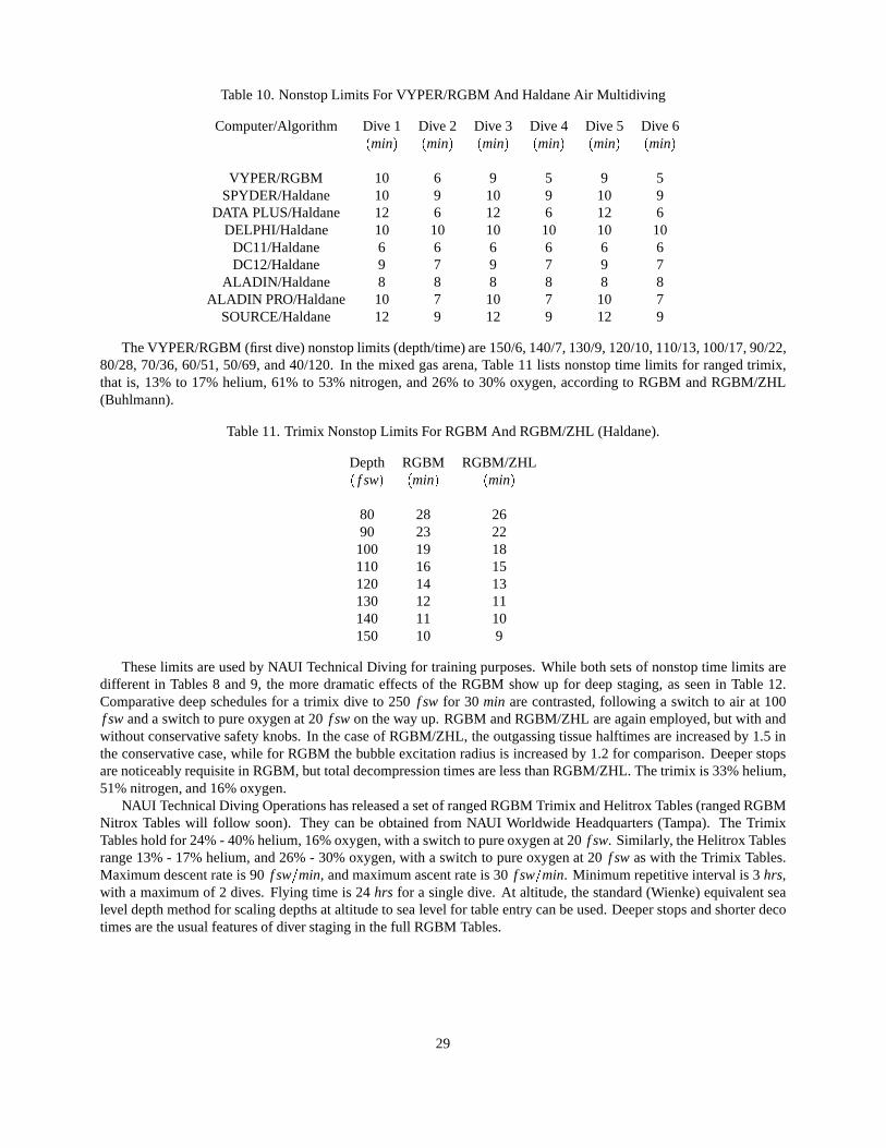
Table 10. Nonstop Limits For VYPER/RGBM And Haldane Air Multidiving

Computer/Algorithm Dive 1 Dive 2 Dive 3 Dive 4 Dive 5 Dive 6(min) (min) (min) (min) (min) (min)

VYPER/RGBM 10 6 9 5 9 5SPYDER/Haldane 10 9 10 9 10 9

DATA PLUS/Haldane 12 6 12 6 12 6DELPHI/Haldane 10 10 10 10 10 10

DC11/Haldane 6 6 6 6 6 6DC12/Haldane 9 7 9 7 9 7

ALADIN/Haldane 8 8 8 8 8 8ALADIN PRO/Haldane 10 7 10 7 10 7

SOURCE/Haldane 12 9 12 9 12 9

The VYPER/RGBM (first dive) nonstop limits (depth/time) are 150/6, 140/7, 130/9, 120/10, 110/13, 100/17, 90/22,80/28, 70/36, 60/51, 50/69, and 40/120. In the mixed gas arena, Table 11 lists nonstop time limits for ranged trimix,that is, 13% to 17% helium, 61% to 53% nitrogen, and 26% to 30% oxygen, according to RGBM and RGBM/ZHL(Buhlmann).

Table 11. Trimix Nonstop Limits For RGBM And RGBM/ZHL (Haldane).

Depth RGBM RGBM/ZHL( f sw) (min) (min)

80 28 2690 23 22

100 19 18110 16 15120 14 13130 12 11140 11 10150 10 9

These limits are used by NAUI Technical Diving for training purposes. While both sets of nonstop time limits aredifferent in Tables 8 and 9, the more dramatic effects of the RGBM show up for deep staging, as seen in Table 12.Comparative deep schedules for a trimix dive to 250 f sw for 30 min are contrasted, following a switch to air at 100f sw and a switch to pure oxygen at 20 f sw on the way up. RGBM and RGBM/ZHL are again employed, but with andwithout conservative safety knobs. In the case of RGBM/ZHL, the outgassing tissue halftimes are increased by 1.5 inthe conservative case, while for RGBM the bubble excitation radius is increased by 1.2 for comparison. Deeper stopsare noticeably requisite in RGBM, but total decompression times are less than RGBM/ZHL. The trimix is 33% helium,51% nitrogen, and 16% oxygen.

NAUI Technical Diving Operations has released a set of ranged RGBM Trimix and Helitrox Tables (ranged RGBMNitrox Tables will follow soon). They can be obtained from NAUI Worldwide Headquarters (Tampa). The TrimixTables hold for 24% - 40% helium, 16% oxygen, with a switch to pure oxygen at 20 f sw. Similarly, the Helitrox Tablesrange 13% - 17% helium, and 26% - 30% oxygen, with a switch to pure oxygen at 20 f sw as with the Trimix Tables.Maximum descent rate is 90 f sw=min, and maximum ascent rate is 30 f sw=min. Minimum repetitive interval is 3 hrs,with a maximum of 2 dives. Flying time is 24 hrs for a single dive. At altitude, the standard (Wienke) equivalent sealevel depth method for scaling depths at altitude to sea level for table entry can be used. Deeper stops and shorter decotimes are the usual features of diver staging in the full RGBM Tables.

29

Table 12. Deep Schedules According To RGBM And RGBM/ZHL (Haldane)

Depth RGBM/ZHL RGBM RGBM/ZHL RGBM( f sw) (min) (min) (min) (min)

Stop (standard) (standard) (sa f er) (sa f er)

1 180 0 0 0 12 170 0 1 0 13 160 0 1 0 14 150 0 1 0 15 140 0 1 0 26 130 0 2 0 27 120 0 2 0 28 110 0 2 1 29 100 0 2 2 2

10 90 2 2 3 311 80 2 2 4 312 70 2 3 5 413 60 5 5 8 614 50 7 6 12 715 40 12 9 18 1916 30 18 12 28 1317 20 16 10 28 1118 10 28 16 48 18

93 77 147 98

That in a nutshell is a comparison of major differences between phase and dissolved gas models. The phase modelsrecover dissolved gas models for short and nominal exposures, but require deeper stops and shorter decompressiontimes for longer and exceptional exposures. A rundown of the software configuration of the RGBM used in full blownsimulations follows. The package is under constant refinement and updating.

1. Module: Three major routines (RGBMNX, RGBMHX, RGBMTMX) for nitrox, heliox, and trimix.

2. Source Code: 1640 Lines

3. Language/Compiler: FORTRAN 77/90, BASIC.

4. CRAY YMP Running Time: 1 sec for deep trimix profile with 5 gas switches on way up.

5. Input: altitude, bottom mixture, ascent/descent rate, switch levels and gas mixtures, predive breathing gas, safetyknobs, previous dive history.

6. Output: controlling tissue compartments, stop depth and times, supersaturation gradient, permissble supersatura-tion, effective bubble and gas parameters, critical phase volume, dive profile.

7. Cost: $5800

Diving ConservatismIn finishing, a few clinical observations are listed, not to scare the reader, but rather to point out that diving, like

all other environmentally changing activities, has its own set of risk factors. Risk, obviously here, relates to pressurechanges and exposure times:

1. in 1976, Palmer and Blakemore reported that 81% of goats with CNS bends and 33% with limb bends exhibitedpermanent spinal cord damage on autopsy;

30

2. in 1978, the same investigators reported that clinically bent, but cured, goats, also exhibited brain damage onautopsy;

3. in 1979, a Workshop in Luxemborg reported that even asymptomatic dives may cause permanent brain and spinalimpairment;

4. in 1982, Idicula reported CT scans of the brains of veteran divers showed characteristics similar to punch drunkdivers;

5. in 1984, Edmonds conducted physchological and psychometric studies on abalone divers in Australia and reportedstrong evidence for dementia;

6. in 1985, Hoiberg reported the USN divers who once suffered the bends had a higher rate of headaches, vasculardiseases, and hospitalizations than a matched sample who had never been bent;

7. in 1986, Morris reported that English divers with more than 8 years experience has significantly poorer short termmemory;

8. in the 1980s and 1990s, Workshops repeatedly voiced concern about the long term effects of transient hematolog-ical changes in divers, such as sedimentation, red cell configuration, alteration of lipoprotein, platelet reduction,and vascular stress;

9. in 1984, Brubakk noted ultrasonically detected bubbles (VGE) in animals for as long as a month after hyperbaricexposure;

10. now, Calder examines the spinal cord of every diver in the United Kingdom who dies of any cause;

11. in 1985, Dick reported that mild (self) neurological complaints are common after diving and go untreated, andthat many serious cases never violated the USN Tables.

Of course, it comes as no surprise that the medical community continues to push for shorter and shallower exposures,ultra conservatism in tables and meters, and all other risk ameliorating avenues. Enough said here, the above list pointsout some concerns for all of us.

Conservative approaches, coupled with the most correct biophysical models, are the best means for staging diverascents. Period.

Reduced Gradient Bubble Model Validation And TestingModels need validation and testing. Often, strict chamber tests are not possible, economically nor otherwise, and

models employ a number of benchmarks and regimens to underscore viability. The following are some supporting theRGBM phase model and (released) nitrox, heliox, and trimix diving tables:

1. counterterror and countermeasures (LANL) exercises have used the RGBM (full up iterative deep stop version)for a number of years, logging some 450 dives on mixed gases (trimix, heliox, nitrox) without incidence of DCI –35% were deco dives, and 25% were repets (no deco) with at least 2 hr SIs, and in the forward direction (deepestdives first);

2. NAUI Technical Diving has been diving the deep stop version for the past 4 yrs, some estimated 900 dives, onmixed gases down to 250 f sw, without a single DCI hit. Some 15 divers, Fall of 1999, in France used the RGBMto make 2 mixed gas dives a day, without mishap, in cold water and rough seas. In Roatan, similar week longdecompression diving activities have been logged for the past three years;

3. modified RGBM recreational algorithms (Haldane imbedded with bubble reduction factors limiting reverse pro-file, repetitive, and multiday diving), as coded into Suunto, ABYSS, HydroSpace decometers, lower an alreadylow DCI incidence rate of approximately 1/10,000 or less. More RGBM decompression meters, including mixedgases, are in the works (3 not named at this time). Some 200,000 dives are estimated using RGBM meters, withonly 1 reported case of DCI;

31

4. a cadre of divers and instructors in mountainous New Mexico, Utah, and Colorado have been diving the modified(Haldane imbedded again) RGBM at altitude, an estimated 350 dives, without peril. Again, not surprising sincethe altitude RGBM is slightly more conservative than the usual Cross correction used routinely up to about 8,000ft elevation, and with estimated DCI incidence less than 1/10,000;

5. within decometer implementations of the RGBM, not a single DCI hit has been reported in nonstop and multi-diving categories, beyond 200,000 dives or more, up to now;

6. extreme chamber tests for mixed gas RGBM are in the works, and less stressful exposures will be addressedshortly – extreme here means 300 f sw and beyond;

7. probabilistic decompression analysis of some selected RGBM profiles, calibrated against similar calculations ofthe same profiles by Duke, help validate the RGBM on a computational basis , suggesting that the RGBM has nomore theoretical risk than other bubble or dissolved gas models (Weathersby, Vann, Gerth methodology at USNand Duke).

8. all divers and instructors using RGBM decometers, tables, or NET software have been advised to report individualprofiles to DAN Project Dive Exploration (Vann, Gerth, Denoble and many others at Duke).

9. ABYSS is a NET sotware package that offers the modified RGBM (folded over the Buhlmann ZHL) and soonthe full up, deep stop version for any gas mixture, has a fairly large contingent of tech divers already using theRGBM and has not received any reports of DCI.

10. outside of proprietary (commercial) and RGBM Tables, mixed gas tables are a smorgasboard of no longer ap-plicable Haldane dynamics and discretionary stop insertions, as witnessed by the collective comments of a veryvocal and extremely competent, experienced technical diving community.

Because DCI is binomially distributed in incidence probability, many trials are often needed (or other close profiles)to fully validate any model at the 1% level. Additionally, full validation requires DCI incidences, the higher the number,the better, contrary to desired dive outcomes.

Oxygen Dose And ToxicityDecompression sickness could be avoided by breathing just pure oxygen. And the usage of higher concentrations

of oxygen in breathing mixtures not only facilitates metabolic function, but also aids in the washout of inert gases suchas nitrogen and helium. Despite the beneficial effects of breathing oxygen at higher concentrations, oxygen provesto be toxic in excessive amounts, and over cumulative time intervals. Too little oxygen is equally detrimental to thediver. As discussed, limits to oxygen partial pressures in breathing mixtures range, 0.16 atm to 1.6 atm, roughly, butsymptoms of hypoxia and hyperoxia are dose dependent. Or, in other words, symptom occurences depend on oxygenpartial pressures and exposure times, just like inert gas decompression sickness. The mixed gas diver needs to payattention not only to helium and nitrogen in staged decompression, but also cumulative oxygen exposure over the dive,and possibe underexposure on oxygen depleted breathing mixtures.

The neurotoxic actions of high pressure oxygen are thought to relate directly to biochemical oxidation of enzymes,either those linked to membrane permeability or metabolic pathways. The list below is not exhaustive, but includes thefollowing mechanisms:

1. the inability of blood to remove carbon dioxide from tissue when hemoglobin is oxygen saturated;

2. inhibition of enzymes and coenzymes by lipid peroxides;

3. increased concentration of chemical free radicals which attack cells:

4. oxidation of membranes and structural deterioration reducing electrical permeability for neuron activation:

5. direct oxygen attack on smooth muscle fibres;

6. oxygen induced vasoconstriction in arterioles;

7. elevation of brain temperature due to lack of replacement of oxygen by carbopn dioxide in hemoglobin;

32

8. and, simple chemical kinetic redistribution of cellular carbon dioxide and oxygen with high surrounding oxygentensions.

Fortunately for the diver, there are ways to avoid complications of hyperoxia. Careful attention to dose (depth-time)limitations for oxygen exposures is needed.

Despite the multiplicity and complexity of the above, limits for safe oxygen exposure are reasonably defined. Table13 below lists NOAA oxygen exposure time limits, tx, for corresponding oxygen partial pressures, pO2 . Below 0.5 atm,oxygen toxicity is not really a problem.

Table 13. Oxygen Dose-Time Limits

oxygen partial pressure oxygen time limit oxygen tolerance (OTU)pO2 (atm) tx (min) ϒ(min)

1.6 45 871.5 120 2131.4 150 2441.3 180 2661.2 210 2781.1 240 2791.0 300 3000.9 360 2990.8 450 2950.7 570 2660.6 720 189

The data in Table 13 is easily fitted to a dose time curve, using least squares, yielding,

tx = exp

3:0 pO2

:36

= 4160 exp (2:77pO2) (127)

or, equivalently,pO2 = 3:0 :36 ln (tx) (128)

in the same units, that is pO2 and tx in atm and min respectively. The last column tabulates an exposure dose, ϒ, fordivers, called the oxygen tolerance unit (OTU), developed by Lambertsen and coworkers at the University of Pennsyl-vania. Formally, the oxygen toxicity, ϒ, is given by,

ϒ=

pO2 0:5

0:5

0:83

t (129)

and can be cumulatively applied to diving exposures according to the following prescriptions:

1. maintain single dive OTUs below 750 min on the liberal side, or allow for 550 min of that as possible full DCIrecompression treatment on the conservative side;

2. maintain repetitive total dive OTUs below 300 min.

The expression is applied to each and all segments of a dive, and summed accordingly for total OTUs, and then bench-marked against the 750 min or 300 min rough rule. The 750 min and 300 min OTU rules are not cast in stone in thediving community, and 10% to 25% variations are common, in both conservative and liberal directions.

For exceptional and multiple exposures, the USN and University of Pennslyvania suggest the limits summarized inTable 14, where for multiple exposures, N, and segment times, txn ,

Tx =N

∑n=1

txn (130)

33

Table 14. Oxygen Exceptional Exposure Time Limits

oxygen partial pressure single exposure multiple exposurespO2 (atm) tx (min) Tx (min)

2.0 301.9 451.8 601.7 751.6 120 151.5 150 1801.4 180 1801.3 240 2101.2 270 2401.1 300 2700.9 360 3600.8 450 4500.7 570 5700.6 720 720

Note the severe reduction in multiple oxygen exposure time at 1.6 atm in Table 14. For this reason, technical diversgenerally restrict mixed gas diving exposures to pO2 1:6 atm throughout any sequence of dives.

There are many ways to measure oxygen, with devices called oxygen analyzers. They are employed in chemi-cal plants and refineries, hyperbaric chambers, intensive care units, and nurseries. The paramagnetic analyzer is veryaccurate, and relies on oxygen molecular response to a magnetic field in displacing inert gases from collection cham-bers. Thermal conductivity analyzers differentiate oxygen and nitrogen conduction properties in tracking temperaturesin thermistors, with difference in temperatures proportional to the oxygen concentration. Magnetic wind analyzerscombine properties of paramagnetic and thermal analyzers. Polarographic analyzers measure oxygen concentrationby resistance changes across permeable oxygen membranes. Galvanic cell analyzers are microfuel cells, consumingoxygen on touch and generating a small current proportional to the amount of oxygen consumed. In all cases, analyzerresponse is linear in oxygen concentration.

Although it is tempting to avoid problems of oxygen toxicity by maintaining oxygen partial pressures, pO2 , far belowtoxic limits, this is not beneficial to inert gas elimination (free or dissolved state). Higher levels of inspired oxygen, thuscorrespondingly lower levels of inert gases, are advantageous in minimizing inert gas buildup and maximizing inert gaswashout. Coupled to narcotic potency of helium and nitrogen, and molecular diffusion rates, balancing and optimizingbreathing mixtures with decompression requirements is truly a complex and careful technical diving exercise.

ADDITIONAL READING

References span a wide spectra of technical diving material and details, broaching historical to modern develop-ments. Entries are alphabetically and chronologically listed.

Abramowitz M. and Stegun I.A., 1972, Handbook Of Mathematical Functions, New York: Dover Publications.

Berghage T.E. and Durman D., 1980, US Navy Air Recompression Schedule Risk Analysis, Nav. Med. Res. Bull. 1,1-22.

Bowker A.H. and Lieberman G.J., 1964, Engineering Statistics, Engelwood Cliffs: Prentice-Hall.

Boycott A.E., Damant G.C.C., and Haldane J.S., 1908, The Prevention Of Compressed Air Illness, J. Hyg. 8, 342-443.

Buhlmann A.A., 1984, Decompression/Decompression Sickness, Berlin: Springer Verlag.

Gernhardt M.L., Lambertsen C.J., Miller R.G., and Hopkins E., 1990, Evaluation Of A Theoretical Model Of TissueGas Phase Growth And Resolution During Decompression From Air Diving, Undersea Biomed. Res. 17, 95.

Hamilton R.W., 1975, Development Of Decompression Procedures For Depths In Excess Of 400 Feet, Undersea AndHyperbaric Medical Society Report, WS: 2-28-76, Bethesda.

34

Hempleman H.V., 1952, A New Theoretical Basis For The Calculation Of Decompression Tables, Medical researchCouncil Report, UPS 131, London.

Hennessy T.R. and Hempleman H.V., 1977, An Examination Of The Critical Released Gas Concept In DecompressionSickness, Proc. Royal Soc. London B197, 299-313.

Hills B.A., 1977, Decompression Sickness, New York: John Wiley And Sons.

Le Messurier D.H. and Hills B.A., 1965, Decompression Sickness: A Study Of Diving Techniques In The Torres Strait,Hvaldradets Skrifter 48, 54-84.

Neal J.G., O’Leary T.R. and Wienke B.R., 1999, Trimix Diving, Fort Lauderdale: Underwater Dynamics Incorporated.

Nishi R.Y., Eatock B.C., Buckingham I.P. and Ridgewell B.A., 1982, Assessment Of Decompression Profiles By Ultra-sonic Monitoring: No Decompression Dives, Defense And Civil Institute Of Environmental Medicine Report, D.C.IEM82-R-38, Toronto.

Parzen E., 1970, Modern Probability Theory And Its Applications, New York: John Wiley And Sons.

Powell R.P.and Rogers R.E., 1989, Doppler Ultrasound Monitoring Of Gas Phase Formation And Resolution In Repet-itive Diving, Undersea Biomed. Res. 16, 69.

Vann R.D., Dovenbarger J., Wachholz C., and Bennett P.B., 1989, Decompression Sickness In Dive Computer And TableUse, DAN Newsletter 3-6.

Vann R.D., Grimstad J., and Nielsen C.H., 1980, Evidence For Gas Nuclei In Decompressed Rats, Undersea Biomed.Res. 7, 107-112.

Weathersby P.K., Survanshi S. and Homer L.D., 1985, Statistically Based Decompression Tables: Analysis Of StandardAir Dives, 1950-1970, Naval Medical Research Institute report, NMRI 85-16, Bethesda.

Weathersby P.K., Homer L.D., and Flynn E.T., 1984, On The Likelihood Of Decompression Sickness, J. Appl. Physiol.57, 815-825.

Wienke B.R., 1993, Diving Above Sea Level, Flagstaff: Best.

Wienke B.R., 1994, Basic Diving Physics And Applications, Flagstaff: Best.

Wienke B.R., 1992, Numerical Phase Algorithm For Decompression Computers And Application, Comp. Biol. Med. 22,389-406.

Wienke B.R., 1991, Basic Decompression Theory And Application, Flagstaff: Best.

Wienke B.R., 1990, Reduced Gradient Bubble Model, Int. J. Biomed. Comp. 26, 237-256.

Wienke B.R., 1986, DECOMP: Computational Package For Nitrogen Transport Modeling In Tissues, Comp. Phys.Comm. 40, 327-336.

Workman R.D., 1965, Calculation Of Decompression Schedules For Nitrogen-Oxygen And Helium-Oxygen Dives, USNExperimental Diving Unit Report, NEDU 6-65, Washington DC

Yount D.E. and Hoffman DC, 1986, On The Use Of A Bubble Formation Model To Calculate Diving Tables, Aviat.Space Environ. Med. 57, 149-156.

Yount D.E., 1979, Skins Of Varying Permeability: A Stabilization Mechanism For Gas Cavitation Nuclei, J. Acoust.Soc. Am. 65, 1431-1439.

Yount D.E. and Strauss R.H., 1976, Bubble Formation In Gelatin: A Model For Decompression Sickness, J. Appl. Phys.47, 5081-5089.

BIOSKETCHES

Bruce Wienke is a Program Manager in the Nuclear Weapons Technology/ Simulation And Computing Office at theLos Alamos National Laboratory (LANL), with interests in computational decompression and models, gas transport,and phase mechanics. He authored Physics, Physiology And Decompression Theory For The Technical And CommercialDiver, High Altitude Diving, Basic Diving Physics And Applications, Diving Above Sea Level, Basic DecompressionTheory And Application, and some 200 technical journal articles. Diving environs include the Caribbean, South Pacific,

35

Asia, inland and coastal United States, Hawaii, and polar Arctic and Antarctic in various technical, scientific, military,and recreational activities. He functions on the LANL Nuclear Emergency Strategy Team (NEST), in exercises ofteninvolving Special Operations Units, above and underwater. He heads Southwest Enterprises, a consulting company forcomputer research and applications in wide areas of applied science and simulation.

He is an Instructor Trainer/Technical Instructor with the National Association Of Underwater Instructors (NAUI),serves on the Board Of Directors (Vice Chairman for Technical Diving, Technical and Decompression Review BoardMember), is a Master Instructor with the Professional Association Of Diving Instructors (PADI) in various capacities(Instructor Review Committee), is an Institute Director with the YMCA, and is an Instructor Trainer/Technical Instructorwith Scuba Diving International/Technical Diving International (SDI/TDI).

Wienke, a former dive shop owner in Santa Fe, presently works with DAN on applications of high performancecomputing and communications to diving, and is a Regional Data Coordinator for Project Dive Exploration. Scubapro,Suunto, Abysmal Diving, HydroSpace Engineering, and Atomic Aquatics engage (or have) him as Consultant for meteralgorithms. He is the developer of the Reduced Gradient Bubble Model (RGBM), a dual phase approach to stagingdiver ascents over an extended range of diving applications (altitude, nonstop, decompression, multiday, repetitive,multilevel, mixed gas, and saturation). The Suunto VYPER/COBRA/STINGER dive computers incorporate the RGBMinto staging regimens, particularly for recreational diving (including nitrox). The HydroSpace EXPLORER employsthe RGBM for mixed gases and decompression diving across recreational and technical diving activities. ABYSS, acommercial software product, features some of the RGBM dynamical diving algorithms developed by him for Internetusers and technical divers. He is also Associate Editor for the International Journal Of Aquatic Research And Education,and is a former Contributing Editor of Sources, the NAUI Training Publication.

Wienke received a BS in physics and mathematics from Northern Michigan University, an MS in nuclear physicsfrom Marquette University, and a PhD in particle physics from Nothwestern University. He is a member of the Under-sea And Hyperbaric Medical Society (UHMS), American Physical Society (APS), Society Of Industrial And AppliedMathematics (SIAM), and the American Academy Of Underwater Sciences (AAUS).

Bruce WienkeLos Alamos National Laboratory

Los Alamos, N.M. 87545(505) 667-1358

brw@lanl.gov

Tim O’Leary is Director of NAUI Worldwide Technical Training Operations, Course Director for NAUI Worldwide,Inspector Trainer for PSI, and President of American Diving And Marine Salvage. He has spoken at many underwatersymposiums, as well as contributing to recreational and technical periodicals.

He has dived in Asia, South Pacific, North Sea, Mediteranian, Mexico, Central and South America, and the UnitedStates as both a mixed gas Commercial Diver and technical diving Instructor Trainer.

O’Leary received a BS in zoology from Texas AM University, a DMT and CHT from Jo Ellen Smith MedicalCeneter at the Baromedical Research Institute. He has worked as a Commercial Diving Instructor at the Ocean Corpo-ration, a Saturation Diver, Gas Rack Operator, Saturation Supervisor, and Chamber Supervisor for many of the world’scommercial diving companies. He currently serves as a Consultant for the offshore oil industry, and is a Level III NDTTechnician.

O’Leary is a member of the Undersea And Hyperbaric Medical Society (UHMS), Society Of Naval Architects AndMarine Engineers (SNAME), National Association Of Diver Medical Technicians (NADMT), and is an Admiral in theTexas Navy.

Tim O’LearyAmerican Diving And Marine Salvage

1807 Padre BoulevardSouth Padre Island, Tx. 78597

(800) 761-2030Nauitec@aol.com

36