Revista Mexicana de Astronomía y Astrofísica

ISSN: 0185-1101

rmaa@astroscu.unam.mx

Instituto de Astronomía

México

Avila, R.; Ibañez, F.; Vernin, J.; Masciadri, E.; Sánchez, L. J.; Azouit, M.; Agabi, A.; Cuevas, S.;

Garfias, F.

Optical-turbulence and wind profiles at San Pedro Mártin

Revista Mexicana de Astronomía y Astrofísica, vol. 19, abril, 2003, pp. 11-22

Instituto de Astronomía

Distrito Federal, México

Disponible en: http://www.redalyc.org/articulo.oa?id=57101904

Cómo citar el artículo

Número completo

Más información del artículo

Página de la revista en redalyc.org

Sistema de Información Científica

Red de Revistas Científicas de América Latina, el Caribe, España y Portugal

Proyecto académico sin fines de lucro, desarrollado bajo la iniciativa de acceso abierto

San

Ped

ro M

árti

r: A

stro

nom

ica

l Site

Eva

lua

tion

(Mé

xic

o, D

. F. a

nd E

nse

nad

a, B

. C.,

Mé

xic

o, A

pril

3-4

, 200

3)Ed

itors

: Ire

ne C

ruz-

Go

nzá

lez,

Re

my

Avi

la &

Ma

uric

io T

ap

iaRevMexAA (Serie de Conferencias), 19, 11–22 (2003)

OPTICAL-TURBULENCE AND WIND PROFILES AT SAN PEDRO MARTIR

R. Avila,1 F. Ibanez,1 J. Vernin,2 E. Masciadri,3,4 L. J. Sanchez,4 M. Azouit,2 A. Agabi,2 S. Cuevas,4 andF. Garfias4

RESUMEN

Se presentan resultados del monitoreo de perfiles de turbulencia optica y velocidad de las capas turbulentas enSan Pedro Martir, Mexico. Los datos fueron colectados durante 11 noches en abril–mayo 1997 y 16 noches enmayo 2000 utilizando el Scidar Generalizado de la Universidad de Niza instalado en los telescopios de 1.5-m y2.1-m. El analisis estadıstico de los 6414 perfiles de turbulencia obtenidos muestra que la distorsion de la imagen(llamada comunmente seeing) producida por la turbulencia en los primeros 1.2 km, sin incluir la turbulenciade cupula, en los telescopios de 1.5-m y 2.1-m tiene valores medianos de 0.′′63 y 0.′′44, respectivamente. Elseeing de cupula en dichos telescopios tiene valores medianos de 0.′′64 y 0.′′31. La turbulencia por encima de 1.2km y en la atmosfera completa produce seeing con valores medianos de 0.′′38 y 0.′′71. La correlacion temporalde la intensidad de la turbulencia cae a 50% en perıodos de tiempo de 2 y 0.5 horas, aproximadamente,para alturas mayores y menores que 16 km sobre el nivel del mar, respectivamente. La turbulencia arribade ∼9 km permanecio notablemente debil durante 9 noches consecutivas, lo cual es alentador para realizarobservaciones de alta resolucion angular en el sitio. Los 3016 perfiles de la velocidad de las capas turbulentasque son analizados muestran que las capas mas veloces se encuentran entre 10 y 17 km, donde se localizan latropopausa y la corriente de chorro, con velocidad mediana de 24.4 m s−1. El valor mediano del tiempo decoherencia del frente de onda es 6.5 ms, en el visible. Los resultados obtenidos en este trabajo colocan a SanPedro Martir entre los sitios mas adecuados para la instalacion de telescopios opticos de la proxima generacion.

ABSTRACT

Results of monitoring optical–turbulence profiles and velocity of the turbulence layers at San Pedro Martir,Mexico, are presented. The data were collected during 11 nights in April–May 1997 and 16 nights in May 2000using the Generalized Scidar of Nice University installed on the 1.5–m and 2.1–m telescopes. The statisticalanalysis of the 6414 turbulence profiles obtained shows that the seeing produced by the turbulence in the first1.2 km, not including dome seeing, at the 1.5–m and the 2.1–m telescopes have median values of 0.′′63 and0.′′44, respectively. The dome seeing at those telescopes have median values of 0.′′64 and 0.′′31. The turbulenceabove 1.2 km and in the whole atmosphere produces seeing with median values of 0.′′38 and 0.′′71. The temporalcorrelation of the turbulence strength drops to 50% in time lags of 2 and 0.5 hours, approximately, for altitudesbelow and above 16 km above sea level, respectively. The turbulence above ∼9 km remained notably calmduring 9 consecutive nights, which is encouraging for adaptive optics observations at the site. The 3016 profilesof the turbulent–layer velocity that are analyzed show that the fastest layers are found between 10 and 17 km,where the tropopause and the jet stream are located, with median speed of 24.4 m s−1. In the first 2.2 kmand above 17 km, the turbulent layers move relatively slowly, with median speeds of 2.3 and 9.2 m s−1. Themedian of the wavefront coherence–time is 6.5 ms, in the visible. The results obtained here places San PedroMartir among the best suited sites for installing next generation optical telescopes.

Key Words: ATMOSPHERIC EFFECTS — INSTRUMENTATION: ADAPTIVE OPTICS — SITE

TESTING — TURBULENCE

1. INTRODUCTION

The development and operation of ground–basedmodern astronomical facilities achieving high angu-lar resolution observations, require an increasingly

1Centro de Radioastronomıa y Astrofısica, UNAM, More-lia, Mexico

2U. M. R. 6525 Astrophysique, UNSA/CNRS, France3Max Plank Institut fur Astronomie, Heidelberg, Germany4Instituto de Astronomıa, UNAM, Mexico D.F., Mexico

precise characterization of the on site atmosphericturbulence. Fundamental data for such a task arevertical profiles of the optical turbulence, repre-sented by the refractive–index structure constantC2

N(h), and velocity of the turbulent layers V(h).Information about the seeing is necessary but notsufficient. For example, the design of multiconjugateadaptive optics (MCAO) (systems that incorporateseveral deformable mirrors, each conjugated at a dif-

11

San

Ped

ro M

árti

r: A

stro

nom

ica

l Site

Eva

lua

tion

(Mé

xic

o, D

. F. a

nd E

nse

nad

a, B

. C.,

Mé

xic

o, A

pril

3-4

, 200

3)Ed

itors

: Ire

ne C

ruz-

Go

nzá

lez,

Re

my

Avi

la &

Ma

uric

io T

ap

ia12 AVILA ET AL.

ferent altitude) requires knowledge of the statisticalbehavior of the optical–turbulence in the atmospherelike the altitude of the predominant turbulent layers,their temporal variability and the velocity of theirdisplacement. Moreover, the selection of the siteswhere the next–generation ground–based telescopesare to be installed needs reliable studies of the C2

N

and V profiles at those sites.These reasons have motivated the accomplish-

ment of two campaigns aimed at monitoring C2N and

V profiles at the Observatorio Astronomico Nacionalde San Pedro Martir (OAN–SPM). The campaignstook place in 1997 (April and May) and 2000 (May),for a total of 27 nights. Here we present the mainresults obtained from the C2

N(h) and V(h) measure-ments performed during these campaigns. Avila,Vernin, & Cuevas (1998) reported the C2

N(h) resultsfrom the 1997 observations alone. Section 2 brieflypresents the measurement techniques and the obser-vation campaigns. An overview of the monitoredturbulence profiles is given in § 3 and the statisticalanalysis of the C2

N vertical distribution is presentedin § 4. The temporal behavior of C2

N(h) is studied in§ 5. In § 6 the wind profiles and a simple statisticalanalysis is presented. Finally, § 7 gives a summaryof the results.

2. MEASUREMENTS OF C2N AND V PROFILES

The principal method followed to measure theturbulence and velocity profiles at the OAN–SPMhas been that of the Generalized Scidar (GS). De-tails of the instrumental concept, together with acomplete bibliography, can be found in the web pageentitled Generalized Scidar at UNAM 5. Cruz et al.(2003), in this volume, present the development of aGS at UNAM. Here we give a very succinct descrip-tion of the instrument and data reduction procedure.We used the GS developed by Vernin’s group at NiceUniversity (Avila, Vernin, & Masciadri 1997).

The instrumental concept for the determinationof C2

N(h) consists in the measurement of the spa-tial autocorrelation of 1000 to 2000 double–starscintillation–images detected on a virtual plane afew kilometers below the ground. For the determina-tion of the turbulence–layer velocity V(h), the cross–correlation of images delayed by 20 and 40 ms is cal-culated. The exposure time of each image is 1 or 2 msand the wavelength is centered at 0.5 µm. A pair of128×128 autocorrelation and cross–correlation mapsare saved on disk every 1.2 minutes approximately.The double stars used as light sources are listed inTable 1. The data shown in this table were obtained

5http://www.astrosmo.unam.mx/~r.avila/Scidar

TABLE 1

DOUBLE STARS USED FOR THEGENERALIZED SCIDAR

Name α2000a δ2000

a m1b m2

b ρ (′′)c

Castor 7h34 31◦53 1.9 3.0 4.0

γ Leo 10h20 19◦50 2.3 3.6 4.5

ζ UMa 13h24 54◦56 2.2 3.8 14.4

δ Ser 15h35 10◦32 4.2 5.1 4.0

ζ CrB 15h39 36◦38 5.0 5.9 6.4

95 Her 18h01 21◦36 4.8 5.2 6.3aRight ascension (α2000) and Declination (δ2000)bVisible magnitudes of each starcAngular separation

from the Washington Double Star Catalog (Mason,Wycoff, & Hartkopf 2002). Many of the sourcesare multiple systems, but in every case our instru-ment is only sensitive to the primary and secondarycomponents. Using a maximum entropy algorithm,one C2

N profile is retrieved from each autocorrela-tion. The data reduction of the cross–correlationsis performed using an interactive algorithm (Avila,Vernin, & Sanchez 2001). In some cases, the auto-correlation and cross–correlation maps show diago-nal bands parallel to each other. These are producedby video noise on the scintillation images. In suchcases, the maps pass through a filter that eliminatesthe bands prior to do the data reduction. When thenoise is still present after filtering, the maps are re-jected. The vertical resolution of each C2

N profiledepends on the star separation and the zenith an-gle. All the profiles were re-sampled to an altituderesolution of 500 m.

2.1. 1997 Campaign

In the 1997 observing campaign, the GS was in-stalled on the 1.5 m and 2.1 m telescopes (1.5mT and2.1mT) for 8 and 3 nights respectively (1997 March23–30 and April 20–22 UT). Simultaneously, the IA–UNAM differential image motion monitor (DIMM)(Sarazin & Roddier 1990) was used to measure theopen air seeing. The 2.1mT is installed on top ofa 15 meter tall building lying at the summit of themountain (2850 m above sea level) in such a way thatno obstacle can generate ground turbulence. On theother hand, the 1.5mT is constructed closer to theground level, on a site situated below the summit.

San

Ped

ro M

árti

r: A

stro

nom

ica

l Site

Eva

lua

tion

(Mé

xic

o, D

. F. a

nd E

nse

nad

a, B

. C.,

Mé

xic

o, A

pril

3-4

, 200

3)Ed

itors

: Ire

ne C

ruz-

Go

nzá

lez,

Re

my

Avi

la &

Ma

uric

io T

ap

iaTURBULENCE AND WIND PROFILES AT SPM 13

2.2. 2000 Campaign

The 2000 campaign took place in May 7 through22, UT. A number of instruments were deployed:

• The GS, installed during 9 and 7 nights (7–15and 16–22 April UT) on the 1.5mT and 2.1mTtelescopes, respectively.

• Instrumented balloons, launched to senseone detailed C2

N profile per night. The balloonlaunches require quiet wind conditions or a largearea clear of obstacles in case of windy condi-tions. Trees and buildings of the observatorysite prevented us from launching balloons whenthe wind was strong. In these cases, balloonswere launched from Vallecitos, an area clear oftrees, 3 km away from the observatory and 300m below.

• A 15–m–high mast, equipped with microther-mal sensors – of the same kind as those used onthe balloons – to measure the C2

N values at 7different altitudes up to 15 m (Sanchez et al.2003).

• A DIMM, installed 8 m away from the mast,to monitor the open air seeing.

• Meteorological balloons, to measure the pro-files of T , P , V, and the humidity q. These werelaunched from Colonet, a town on the PacificOcean shore.

The measurements obtained with the mast and theDIMM led to a study of the contribution of the sur-face layer to the seeing. This work is presented bySanchez et al. (2003) in this volume.

Most of the data gathered in this campaign wereused for the calibration of the Meso–NH atmosphericmodel for the 3D simulation of C2

N (Masciadri, Avila,& Sanchez 2003).

3. C2N(h) DATA OVERVIEW

The number of turbulence profiles measured inthe 1997 and the 2000 campaigns are 3398 and 3016,making a total of 6414 estimations of C2

N(h). Fig-ure 1 shows most of the C2

N profiles obtained duringthe 2000 campaign. The aim of that figure is to givethe reader a feeling of the evolution of the turbu-lence profiles during each night and from night tonight. The three upper rows correspond to the dataobtained with the 1.5mT. In the two last rows, thedata obtained with the 2.1mT is represented. Thefirst 2.1mT night was cloudy. The blank zones corre-spond to either technical problems, clouds or changes

TABLE 2

DOME SEEING STATISTICS (arcsec)

Tel. 1stQuartile Median 3rd Quartile

1.5mT 0.55 0.64 0.77

2.1mT 0.23 0.31 0.41

of source. C2N values for altitudes within the obser-

vatory and 1 km lower are to be taken as part ofthe response of the instrument to turbulence at theobservatory level. For altitudes lower than that, theC2

N values are artifacts of the inversion procedure,and should be ignored.

Generally, the most intense turbulence is locatedat the observatory level, where the contributionsfrom inside and outside of the telescope dome areadded. In the statistical analysis, presented in § 4,dome turbulence is subtracted. The profiles obtainedwith the 2.1mT show a fairly stable and stronglayer between 10 and 15 km, corresponding to thetropopause (as deduced from the balloon data). Thislayer is rarely present in the data obtained with the1.5–mT. Sporadic turbulence bursts are noticed ataltitudes higher than 15 km.

4. STATISTICS ON THE C2N

VERTICAL–DISTRIBUTION

4.1. Dome seeing

All the “raw” C2N profiles, as those shown in

Fig. 1, include in the ground layer the turbulenceinside the telescope dome. For the characterizationof the site, we need to remove the dome seeing con-tribution from the profiles. The method followed toestimate the dome C2

N is explained in detail by Avilaet al. (2001) and some improvements are suggestedby Masciadri et al. (2003). The dome seeing was de-termined for 84% of the profiles measured during the2000 campaign. In the remaining 16% of the profiles,the determination of the dome seeing was “ambigu-ous”, so we did not include these data to the domeseeing database. Refer to Avila et al. (2001) for aprecise definition of an “ambiguous” determinationof the dome seeing.

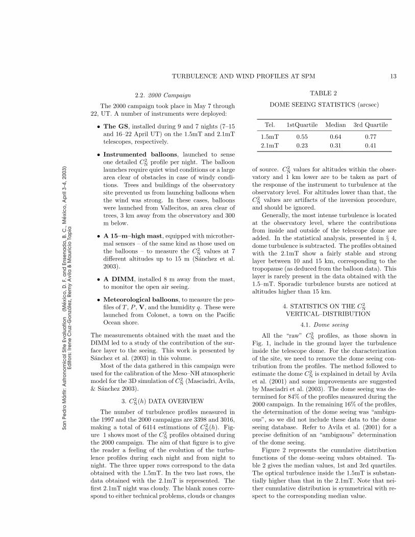
Figure 2 represents the cumulative distributionfunctions of the dome–seeing values obtained. Ta-ble 2 gives the median values, 1st and 3rd quartiles.The optical turbulence inside the 1.5mT is substan-tially higher than that in the 2.1mT. Note that nei-ther cumulative distribution is symmetrical with re-spect to the corresponding median value.

San

Ped

ro M

árti

r: A

stro

nom

ica

l Site

Eva

lua

tion

(Mé

xic

o, D

. F. a

nd E

nse

nad

a, B

. C.,

Mé

xic

o, A

pril

3-4

, 200

3)Ed

itors

: Ire

ne C

ruz-

Go

nzá

lez,

Re

my

Avi

la &

Ma

uric

io T

ap

ia14 AVILA ET AL.

Fig. 1. Mosaic of the turbulence profiles measured during the whole campaign. Each box corresponds to one night. Thevertical and horizontal axis represent the altitude (in km) above sea level and the universal time (in hours), respectively.TheC2

N values are coded in the color scale shown on the right–hand side of each box. The three upper rows and the twobottom rows contain the profiles obtained at the 1.5 mT and 2.1 mT, respectively. Time increases in the left–right andup–down directions. The white line centered at 2.8 km indicates the observatory altitude.

San

Ped

ro M

árti

r: A

stro

nom

ica

l Site

Eva

lua

tion

(Mé

xic

o, D

. F. a

nd E

nse

nad

a, B

. C.,

Mé

xic

o, A

pril

3-4

, 200

3)Ed

itors

: Ire

ne C

ruz-

Go

nzá

lez,

Re

my

Avi

la &

Ma

uric

io T

ap

iaTURBULENCE AND WIND PROFILES AT SPM 15

Fig. 2. Cumulative distribution of the seeing generatedinside the dome of the 2.1mT (full line) and the 1.5mT(dashed line). The vertical and horizontal lines indicatethe median values. These values together with the 1stand third quartiles are reported in Table 2.

In the remaining part of the paper, all the sta-tistical results concerning the turbulence near theground are free of dome–turbulence.

4.2. Median profiles

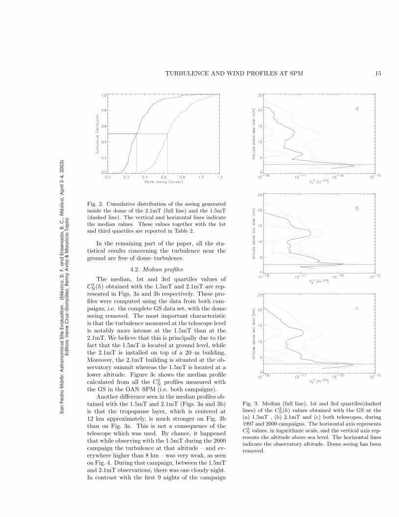
The median, 1st and 3rd quartiles values ofC2

N(h) obtained with the 1.5mT and 2.1mT are rep-resented in Figs. 3a and 3b respectively. These pro-files were computed using the data from both cam-paigns, i.e. the complete GS data set, with the domeseeing removed. The most important characteristicis that the turbulence measured at the telescope levelis notably more intense at the 1.5mT than at the2.1mT. We believe that this is principally due to thefact that the 1.5mT is located at ground level, whilethe 2.1mT is installed on top of a 20–m building.Moreover, the 2.1mT building is situated at the ob-servatory summit whereas the 1.5mT is located at alower altitude. Figure 3c shows the median profilecalculated from all the C2

N profiles measured withthe GS in the OAN–SPM (i.e. both campaigns).

Another difference seen in the median profiles ob-tained with the 1.5mT and 2.1mT (Figs. 3a and 3b)is that the tropopause layer, which is centered at12 km approximately, is much stronger on Fig. 3bthan on Fig. 3a. This is not a consequence of thetelescope which was used. By chance, it happenedthat while observing with the 1.5mT during the 2000campaign the turbulence at that altitude – and ev-erywhere higher than 8 km – was very weak, as seenon Fig. 4. During that campaign, between the 1.5mTand 2.1mT observations, there was one cloudy night.In contrast with the first 9 nights of the campaign

Fig. 3. Median (full line), 1st and 3rd quartiles(dashedlines) of the C

2N(h) values obtained with the GS at the

(a) 1.5mT , (b) 2.1mT and (c) both telescopes, during1997 and 2000 campaigns. The horizontal axis representsC

2N values, in logarithmic scale, and the vertical axis rep-

resents the altitude above sea level. The horizontal linesindicate the observatory altitude. Dome seeing has beenremoved.

San

Ped

ro M

árti

r: A

stro

nom

ica

l Site

Eva

lua

tion

(Mé

xic

o, D

. F. a

nd E

nse

nad

a, B

. C.,

Mé

xic

o, A

pril

3-4

, 200

3)Ed

itors

: Ire

ne C

ruz-

Go

nzá

lez,

Re

my

Avi

la &

Ma

uric

io T

ap

ia16 AVILA ET AL.

Fig. 4. Similar to Fig. 3 but for the GS profiles obtainedat the 1.5mT during the 2000 campaign.

(when the GS was installed on the 1.5mT), duringthe first observable night on the 2.1mT, the turbu-lence in the tropopause was extremely intense. Thiscan be seen on the first box of the 4th row of Fig. 1.It is generally believed that the turbulence intensityat the tropopause is strong due to a dramatic in-crease of the overall vertical gradient of the potentialtemperature and the commonly high–velocity wind(jet stream) in that zone of the atmosphere. How-ever, new evidence that contradicts this speculation– or at least that suggests a more complicated phe-nomenon – is emerging, which motivates a deeperinvestigation. A first step could be to gather a morecomplete statistical data set. For the moment, wenote that 32% of the profiles measured at the OAN–SPM do not show a significant optical turbulence atthe tropopause.

4.3. Seeing for different atmospheric slabs

From a visual examination of Fig. 1, we can de-termine five altitude slabs that contain the predom-inant turbulent layers. These are [2;4], [4;9], [9;16],[16;21] and [21;25] km above sea level. In each al-titude interval of the form [hl;hu] (where the sub-scripts l and u stand for “lower” and “upper” lim-its) and for each profile, we calculate the turbulencefactor

Jhl;hu=

∫ hu

hl

dh C2N(h), (1)

and the correspondent seeing in arc seconds:

εhl;hu= 1.08 × 106λ−1/5J

3/5

hl;hu. (2)

For the turbulence factor corresponding to theground layer, J2;4, the integral begins at 2 km in or-der to include the complete C2

N peak that is due to

Fig. 5. Cumulative distributions of the seeing generatedin different atmosphere slabs: (a) [2;4] km for the 2.1mT(full line) and the 1.5mT (dashed line) without domeseeing; (b) [4;9] km (full line), [9;16] km (dotted line),[16;21] km (dashed line), [21;25] km (dash–dotted line).The horizontal and vertical lines indicate the median val-ues, which are reported in Table 3.

turbulence at ground level (2.8 km). Moreover, J2;4

does not include dome turbulence. The seeing valueshave been calculated for λ = 0.5 µm. In Fig. 5a thecumulative distribution functions of ε2;4 obtained atthe 1.5mT and the 2.1mT, calculated using the com-plete data set, are shown. As discussed in § 4.2, theturbulence at ground level at the 1.5mT is higherthan that at the 2.1mT. The cumulative distribu-tions of the seeing originated in the four slabs of thefree atmosphere (from 4 to 25 km) are representedin Fig. 5b. The strongest turbulence is encounteredfrom 9 to 16 km, where the tropopause layer is lo-cated. The turbulence at altitudes higher than 16km is fairly weak, which is a fortunate feature for theuse of adaptive optics, because it tends to increasethe corrected field–of–view. Finally, Figs. 6a and 6bshow the cumulative distribution of the seeing pro-duced in the free atmosphere, ε4;25, and in the whole

San

Ped

ro M

árti

r: A

stro

nom

ica

l Site

Eva

lua

tion

(Mé

xic

o, D

. F. a

nd E

nse

nad

a, B

. C.,

Mé

xic

o, A

pril

3-4

, 200

3)Ed

itors

: Ire

ne C

ruz-

Go

nzá

lez,

Re

my

Avi

la &

Ma

uric

io T

ap

iaTURBULENCE AND WIND PROFILES AT SPM 17

TABLE 3

SEEING STATISTICS FOR DIFFERENTATMOSPHERE SLABS (arcsec)

Slab (km) 1st Qa Median 3rd Qa

[2; 4] @ 2.1mTb 0.30 0.44 0.63

[2; 4] @ 1.5mTb 0.38 0.63 0.83

[4; 9] 0.12 0.17 0.27

[9; 16] 0.12 0.24 0.43

[16; 21] 0.05 0.08 0.14

[21; 25] 0.01 0.02 0.04

[2; 25]c 0.52 0.71 0.99a1st and 3rd quartilesbWithout dome seeingcAs if measured at the 2.1mT and without dome seeing(see text)

atmosphere, ε2;25, respectively. The computation ofε2;25 is performed as follows: for each profile of thecomplete data set (both campaigns and both tele-scopes) we calculate J4;25 and add a random num-ber that follows the same log–normal distribution asthat of J2;4 obtained in for the 2.1mT. Then thecorresponding seeing value is calculated using Eq. 2.This way, we obtain a distribution of ε2;25 values asif they were measured using the 2.1mT. The reasonfor doing so, is that the values of ε2;25 that we ob-tain are more representative of the potentialities ofthe site than if we had used the distribution of J2;4

obtained for the 1.5mT. The median values of allthe cumulative distributions presented in this Sec-tion are reported in Table 3.

5. TEMPORAL AUTOCORRELATION

What are the characteristic temporal scales ofthe fluctuations of optical turbulence at different al-titudes in the atmosphere? This question has been ofinterest for a long time, and mostly in recent years, asthe development of Multiconjugate Adaptive Optics(MCAO) require knowledge of the properties of theoptical turbulence in a number of slabs in the atmo-sphere. Racine (1996) studied the temporal fluctu-ations of free atmosphere seeing above Mauna Kea.He computed the seeing values by integrating tur-bulence profiles measured in 1987 by Vernin’s groupfrom Nice University using the scidar technique. TheC2

N profiles did not include the turbulence from thefirst kilometer, because the classical mode of thescidar was employed, as the generalized mode didnot exist at that time. Munoz-Tunon, Varela, &

Fig. 6. Cumulative distributions of the seeing generatedin (a) the free atmosphere (altitude higher than 4 km)and (b) the whole atmosphere, without dome seeing (seetext for details). The horizontal and vertical lines indi-cate the median values, which are reported in Table 3.

Vernin (1992) used DIMM data to study the tempo-ral behavior of the open–air seeing at Roque de LosMuchachos observatory. Finally, Tokovinin, Bau-mont, & Vasquez (2003) presented the temporal au-tocorrelation of the turbulence factor in three repre-sentative slabs of the atmosphere above Cerro TololoInteramerican Observatory, using data obtained withthe recently developed Multi–Aperture ScintillationSensor, which provides C2

N measurements at six al-titudes in the atmosphere.

In this Section we investigate the temporal auto-correlation of the turbulence factors Jhl;hu

, for thefive slabs introduced in § 4.3.

5.1. Methodology

The process of building the appropriate se-quences of Jhl;hu

(ti) values is explained below:Typically, three stars are used as light sources eachnight, in a sequence such that the zenith angle neverexceeds ∼40◦. When changing from one star to the

San

Ped

ro M

árti

r: A

stro

nom

ica

l Site

Eva

lua

tion

(Mé

xic

o, D

. F. a

nd E

nse

nad

a, B

. C.,

Mé

xic

o, A

pril

3-4

, 200

3)Ed

itors

: Ire

ne C

ruz-

Go

nzá

lez,

Re

my

Avi

la &

Ma

uric

io T

ap

ia18 AVILA ET AL.

following, the region of the atmosphere that is sensedby the instrument changes significantly and so C2

N(h)can also change, as shown by Masciadri, Avila, &Sanchez (2002). To avoid the confusion between atemporal and a spatial variation of Jhl;hu

, the se-quences Jhl;hu

(ti) never include data obtained withtwo different stars. From the 2000–campaign data,we built 35 sequences Jhl;hu

(ti) for each of the fivealtitude intervals. The temporal sampling of the tur-bulence profiles depends on the number of scintilla-tion images recorded for the computation of eachprofile, which in turn depends on the source magni-tude. Consequently, each sequence Jhl;hu

(ti) is re-sampled with a regular time–interval of δt = 1.14minutes, which is the mean temporal sampling ofthe C2

N profiles. Moreover, while observing a givensource, the data acquisition may be interrupted. Ifthe interruption is longer than 2δt, then the tempo-ral gap is filled with zero values for Jhl;hu

(ti).

For each altitude interval, the calculation of thetemporal autocorrelation, as a function of the tem-poral lag ∆t, is performed as follows: For each Jhl;hu

sequence labeled s, we first compute

Cs(∆t) =

N∆t,s∑

i=1

(

Js(ti) − Js

) (

Js(ti + ∆t) − Js

)

,

(3)where the product is set equal to zero if eitherJs(ti) = 0 or Js(ti + ∆t) = 0. Js is the mean ofthe nonzero values of Js(ti), and N∆t,s is the num-ber of computed nonzero products, which dependson ∆t and the number of nonzero values of Js(ti) inthe sequence s, and is calculated numerically. Theautocorrelation for each altitude slab is then givenby

Γ(∆t) =A(∆t)

B, where (4)

A(∆t) =1

N∆t

Ns∑

s=1

Cs(∆t), (5)

B =1

N0

Ns∑

s=1

Cs(0) and (6)

N∆t =

Ns∑

s=1

N∆t,s. (7)

Ns is the number of sequences for each altitude inter-val. From the definitions of Cs(∆t) and N∆t (Eqs. 3and 7), it can be noticed that the normalizationfactor B only takes into account nonzero values ofJs(ti).

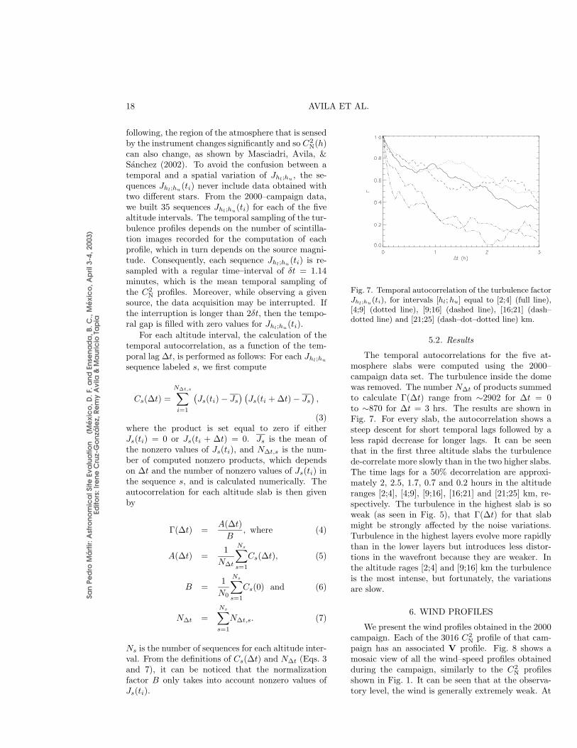
Fig. 7. Temporal autocorrelation of the turbulence factorJhl;hu(ti), for intervals [hl; hu] equal to [2;4] (full line),[4;9] (dotted line), [9;16] (dashed line), [16;21] (dash–dotted line) and [21;25] (dash–dot–dotted line) km.

5.2. Results

The temporal autocorrelations for the five at-mosphere slabs were computed using the 2000–campaign data set. The turbulence inside the domewas removed. The number N∆t of products summedto calculate Γ(∆t) range from ∼2902 for ∆t = 0to ∼870 for ∆t = 3 hrs. The results are shown inFig. 7. For every slab, the autocorrelation shows asteep descent for short temporal lags followed by aless rapid decrease for longer lags. It can be seenthat in the first three altitude slabs the turbulencede-correlate more slowly than in the two higher slabs.The time lags for a 50% decorrelation are approxi-mately 2, 2.5, 1.7, 0.7 and 0.2 hours in the altituderanges [2;4], [4;9], [9;16], [16;21] and [21;25] km, re-spectively. The turbulence in the highest slab is soweak (as seen in Fig. 5), that Γ(∆t) for that slabmight be strongly affected by the noise variations.Turbulence in the highest layers evolve more rapidlythan in the lower layers but introduces less distor-tions in the wavefront because they are weaker. Inthe altitude rages [2;4] and [9;16] km the turbulenceis the most intense, but fortunately, the variationsare slow.

6. WIND PROFILES

We present the wind profiles obtained in the 2000campaign. Each of the 3016 C2

N profile of that cam-paign has an associated V profile. Fig. 8 shows amosaic view of all the wind–speed profiles obtainedduring the campaign, similarly to the C2

N profilesshown in Fig. 1. It can be seen that at the observa-tory level, the wind is generally extremely weak. At

San

Ped

ro M

árti

r: A

stro

nom

ica

l Site

Eva

lua

tion

(Mé

xic

o, D

. F. a

nd E

nse

nad

a, B

. C.,

Mé

xic

o, A

pril

3-4

, 200

3)Ed

itors

: Ire

ne C

ruz-

Go

nzá

lez,

Re

my

Avi

la &

Ma

uric

io T

ap

iaTURBULENCE AND WIND PROFILES AT SPM 19

that altitude, the figures show the speed of the tur-bulence inside the telescope dome, which is zero, andoutside the dome, where the wind is generally slowbut higher than zero. In many cases, dots with dif-ferent colors appear superimposed, which indicatesthe presence of several turbulent layers with altitudedifferences smaller than the vertical resolution of theC2

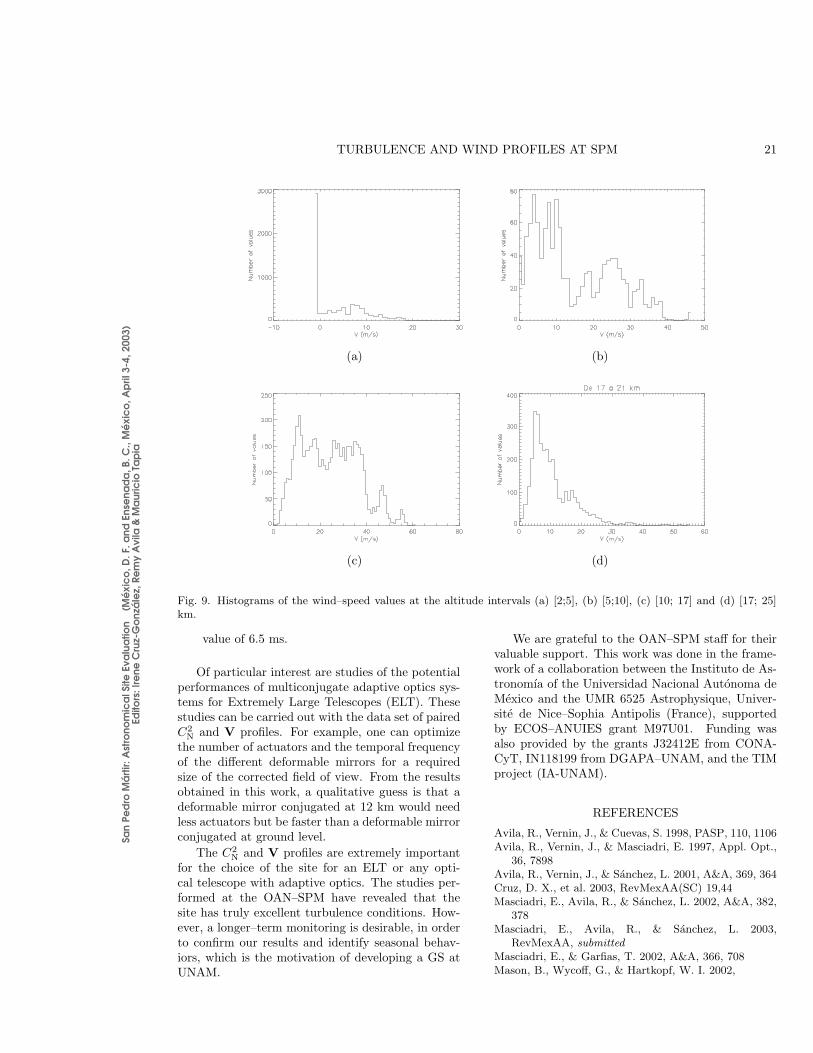
N profiles, but with velocity differences that are de-tectable. The fastest turbulent layers are found be-tween 9 and 16 km. In this altitude range, where thejet stream is located, the wind speed reaches 20 ms−1 only during 7 out of 15 nights. On 2000, May 17UT (4th row, 1st column in Fig. 1), the wind at thataltitude range reached 55 m s−1 and was strongerthan 20 m s−1 all along the night. For altitudeshigher than 16 km, the wind intensity begins to de-crease and above 20 km it is extremely slow. Froma visual inspection of Figs. 1 and 8, it can be seenthat only the night on 2000, May 17 UT and in thejet stream layer, an evident correlation is present be-tween the C2

N and V values. The histograms of thespeed values in the altitude ranges [2;5], [5;10], [10;17] and [17; 25] km are represented in Fig. 9. Thepeak at 0 m s−1 in Fig. 9a is due to the turbulenceinside the dome. The median values in the abovementioned regions of the atmosphere are 2.3 , 11.3,24.4 and 9.2 m s−1, respectively.

From each pair of C2N and V profiles, one can

compute the wavefront coherence–time τ0. The ex-pression given by Roddier, Gilli, & Lund (1982):

τ0 = 0.519

(

2π

λ

)

−5/6 [∫

dh|V(h)|5/3C2N(h)

]

−3/5

(8)corresponds to the coherence time for an ideal full–correction adaptive optics system. The median ofthe τ0 values computed from the 3014 C2

N(h) andV(h) pairs available is 6.5 ms for λ = 0.5 µm. Mas-ciadri & Garfias (2002) made a study of τ0 using C2

N

profiles simulated with the Meso–NH atmosphericmodel, finding similar τ0 values in the summer pe-riod as those found here.

7. SUMMARY AND CONCLUSIONS

Turbulence profiles and velocity of the turbulencelayers have been monitored at the OAN–SPM, dur-ing 11 nights in April–May 1997 and 16 nights inMay 2000. The GS was installed at the foci of the1.5mT and 2.1mT. Turbulence inside the dome is de-tected by the instrument, but for each profile, thiscontribution has been estimated and separated fromthe turbulence near the ground outside the dome.The result is a data set consisting of two subsets:

turbulence profiles free of dome seeing and dome see-ing values. The statistical analysis of this data setlets us draw the following conclusions:

• The turbulence inside the 1.5mT is muchstronger than that at the 2.1mT, with medianvalues of 0.′′64 and 0.′′31.

• The precise location of each telescope influencesthe turbulence measured near the ground. The1.5mT is installed basically at ground level andlower than the site summit, while the 2.1mT ison top of a 20–m building and at the site sum-mit. A consequence of this is that the medianvalues of the seeing produced in the first 1.2 kmare 0.′′63 and 0.′′44 for the 1.5mT and 2.1mT,respectively.

• The seeing generated in the free atmosphere(above 1.2 km from the site), has a median valueof 0.′′38. This very low value encourages adap-tive optics observations, as the lower the tur-bulence in the higher layers, the broader is thecorrected field of view.

• The seeing in the whole atmosphere without thedome contribution as measured from the 2.1mT,has a median value of 0.′′71.

• The temporal autocorrelation of the turbulencefactors Jhl;hu

(see § 4.3) shows that C2N evolves

sensibly more slowly in the layers below 16 km(above see level) than in the layers above thataltitude. The time lag corresponding to a 50%decorrelation is approximately equal to 2 and0.5 hours for turbulence below and above 16km, respectively. The longer the decorrelationtime, the higher the potential performances ofadaptive–optics observations are and the eas-ier would be the development of multiconjugateadaptive optics systems. Rapid evolution of theC2

N in the highest layers is in principle a negativebehavior. However, this is counterbalanced bythe very low C2

N values in those layers. Furtherinvestigations will include the temporal correla-tion of the isoplanatic angle, which would inte-grate both effects.

From the GS data obtained during the 2000 cam-paign, a statistical analysis of the velocity of the tur-bulence layers has been made. The principal resultsand conclusions are the following:

• No evident general correlation between the C2N

value in a layer and the layer speed has beenfound. The correlation is only evident during

San

Ped

ro M

árti

r: A

stro

nom

ica

l Site

Eva

lua

tion

(Mé

xic

o, D

. F. a

nd E

nse

nad

a, B

. C.,

Mé

xic

o, A

pril

3-4

, 200

3)Ed

itors

: Ire

ne C

ruz-

Go

nzá

lez,

Re

my

Avi

la &

Ma

uric

io T

ap

ia20 AVILA ET AL.

Fig. 8. Similar to Fig. 1, but the colors represent wind speed. Each dot indicates one turbulent layer.

one night, in which C2N and V values around 12

km are extremely high. This fact might indi-cate that only for V values higher than a cer-tain threshold level, the C2

N value is correlatedto the V value. Further investigation is neededto prove or disprove this conjecture.

• The fastest layers are found between 10 and 17km, with median speed value of 24.4 m s−1. The

layers above 17 km go notably more slowly (me-dian speed of 9.2 m s−1), which is a positive fea-ture for adaptive optics, because the wavefrontdeformations introduced by those layers wouldbe corrected to a better degree than the lowerlayers, resulting in a wider field of view.

• The wavefront coherence–time for an ideal full–correction adaptive optics system has a median

San

Ped

ro M

árti

r: A

stro

nom

ica

l Site

Eva

lua

tion

(Mé

xic

o, D

. F. a

nd E

nse

nad

a, B

. C.,

Mé

xic

o, A

pril

3-4

, 200

3)Ed

itors

: Ire

ne C

ruz-

Go

nzá

lez,

Re

my

Avi

la &

Ma

uric

io T

ap

iaTURBULENCE AND WIND PROFILES AT SPM 21

(a) (b)

(c) (d)

Fig. 9. Histograms of the wind–speed values at the altitude intervals (a) [2;5], (b) [5;10], (c) [10; 17] and (d) [17; 25]km.

value of 6.5 ms.

Of particular interest are studies of the potentialperformances of multiconjugate adaptive optics sys-tems for Extremely Large Telescopes (ELT). Thesestudies can be carried out with the data set of pairedC2

N and V profiles. For example, one can optimizethe number of actuators and the temporal frequencyof the different deformable mirrors for a requiredsize of the corrected field of view. From the resultsobtained in this work, a qualitative guess is that adeformable mirror conjugated at 12 km would needless actuators but be faster than a deformable mirrorconjugated at ground level.

The C2N and V profiles are extremely important

for the choice of the site for an ELT or any opti-cal telescope with adaptive optics. The studies per-formed at the OAN–SPM have revealed that thesite has truly excellent turbulence conditions. How-ever, a longer–term monitoring is desirable, in orderto confirm our results and identify seasonal behav-iors, which is the motivation of developing a GS atUNAM.

We are grateful to the OAN–SPM staff for theirvaluable support. This work was done in the frame-work of a collaboration between the Instituto de As-tronomıa of the Universidad Nacional Autonoma deMexico and the UMR 6525 Astrophysique, Univer-site de Nice–Sophia Antipolis (France), supportedby ECOS–ANUIES grant M97U01. Funding wasalso provided by the grants J32412E from CONA-CyT, IN118199 from DGAPA–UNAM, and the TIMproject (IA-UNAM).

REFERENCES

Avila, R., Vernin, J., & Cuevas, S. 1998, PASP, 110, 1106Avila, R., Vernin, J., & Masciadri, E. 1997, Appl. Opt.,

36, 7898Avila, R., Vernin, J., & Sanchez, L. 2001, A&A, 369, 364Cruz, D. X., et al. 2003, RevMexAA(SC) 19,44Masciadri, E., Avila, R., & Sanchez, L. 2002, A&A, 382,

378Masciadri, E., Avila, R., & Sanchez, L. 2003,

RevMexAA, submitted

Masciadri, E., & Garfias, T. 2002, A&A, 366, 708Mason, B., Wycoff, G., & Hartkopf, W. I. 2002,

San

Ped

ro M

árti

r: A

stro

nom

ica

l Site

Eva

lua

tion

(Mé

xic

o, D

. F. a

nd E

nse

nad

a, B

. C.,

Mé

xic

o, A

pril

3-4

, 200

3)Ed

itors

: Ire

ne C

ruz-

Go

nzá

lez,

Re

my

Avi

la &

Ma

uric

io T

ap

ia22 AVILA ET AL.

http://ad.usno.navy.mil/wds

Munoz-Tunon, C., Varela, A., & Vernin, J. 1992, A&AS,125, 183

Racine, R. 1996, PASP, 108, 372Roddier, F., Gilli, J., & Lund, G. 1982, J.Opt. (Paris),

Abdelkrim Agabi, Max Azouit and Jean Vernin: U. M. R. 6525 Astrophysique, Universite de Nice SophiaAntipolis/CNRS, Parc Valrose, 06108 Nice Cedex 2, France (karim.agabi,max.azouit,jean.vernin@unice.fr).

Remy Avila, Fabiola Ibanez: Centro de Radioastronomıa y Astrofısica, Universidad Nacional Autonoma deMexico, Campus Morelia, Apartado Postal 3–72, 58090 Morelia, Michoacan, Mexico (r.avila@astrosmo.unam.mx).

Salvador Cuevas, Fernando Garfias and Leonardo J. Sanchez: Instituto de Astronomıa UNAM, Apdo. Postal70–264, 04510 Mexico D.F., Mexico (chavoc,fergar,leonardo@astroscu.unam.mx).

Elena Masciadri: Max Planck Institut fur Astronomie, Konigstuhl 17, D–69117 Heidelberg, Germany(masciadri@mpia.de).

13,263Sanchez, L., et al. 2003, RevMexAA(SC) 19,23Sarazin, M., & Roddier, F. 1990, A&A, 227, 294Tokovinin, A., Baumont, S., & Vasquez, J. 2003, MN-

RAS, 340, 52