Recurrent Bubbles, Economic Fluctuations, andGrowth

Pablo A. Guerron-Quintana, Tomohiro Hirano, and Ryo Jinnai

Boston College and EspolThe University of TokyoHitotsubashi University

RIETI (15 Dec 2017)

Motivation

I Hysteresis and super hysteresis.

I Renewed attention;

I Great Stagnation hypothesis (Hansen, Summers),

I Blanchard, Cerutti, and Summers (2015).

I Bubbles may be important.

I Japan�s lost decades.

I Jorda, Schularick, and Taylor (2015).

I Construct a model; bring it to the data.

Plan

1. Model

2. Comparative Statics

3. Estimation

4. Conclusion

Model

Model

Otherwise standard model with

1. liquidity constraint (Kiyotaki and Moore 2012)

2. variable capacity utilization (Greenwood et. al. 1998),

3. learning-by-doing (Arrow 1962; Sheshinski 1967; Romer 1986).

Liquidity Constraint

I Investors and savers in the economy.

I Investors borrow money using capital as collateral.

I Can�t �nance the total costs due to liquidity constraints.

I Intrinsically useless (liquid) assets may have a positive value.

I Fiat money in Kiyotaki and Moore.

I Bubbles in our model.

Capacity Utilization

I Capital can be intensively used.

I More capital service.

I Faster depreciation.

I Example: road trip in Hokkaido (recommend!).

I pros: fun!

I cons: added mileages lower the used-car value

Learning-By-Doing

I Competitive �rms maximize pro�ts.

I Cobb-Douglas production function

Yt = At|{z}technology level

0@ ut|{z}utilization

Kt

1Aα

(Lt )1�α .

I At is endogenous;

At = A|{z}scale parameter

(Kt )1�α| {z }

externality

.

I Individual �rms take At as exogenous (�Big K, little k� trick).

I Growth is sustained by externality.

Regimes

I Bubble and fundamental regimes.

I M units of bubble assets in bubble regime.

I No bubble assets in fundamental regime.

I Helicopter drop of bubble assets when f ! b.

I Sudden disappearance when b ! f .

I Markov switching.

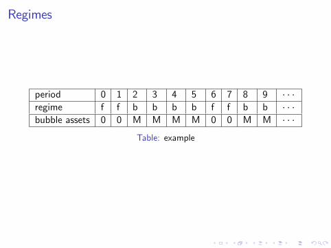
Regimes

period 0 1 2 3 4 5 6 7 8 9 � � �regime f f b b b b f f b b � � �bubble assets 0 0 M M M M 0 0 M M � � �

Table: example

If bubbles arise in the future, why not now?

I We exclude it by assumption.

I No bubble markets in the fundamental regime.

I Neither spot nor future.

I No way to purchase bubble assets (literally).

Comparative Statics

Permanent Fundamental

I Turn o¤ the regime switch for a while.

I Always fundamental.

Fundamental Equilibrium

Non-linear relation when liquidity constraint binds.

Fundamental Equilibrium

Competing e¤ects of a marginal change in liquidity constraint.

Stochastic Bubble

I The economy starts with b.

I Transitions to f with prob. 1% per quarter.

I Stays in f forever (Weil 1987).

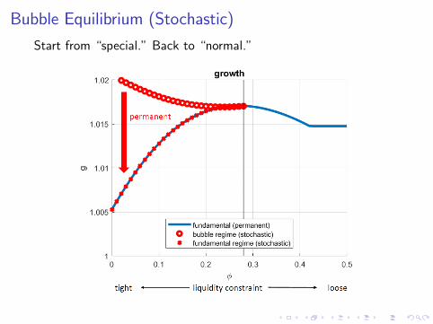
Bubble Equilibrium (Stochastic)

Start from �special.�Back to �normal.�

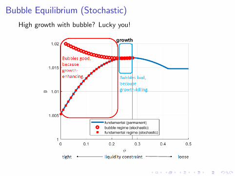
Bubble Equilibrium (Stochastic)

High growth with bubble? Lucky you!

Recurrent Bubble

I Turn on two-way regime switch.

I Both b ! f and f ! b with prob. 1% quarterly.

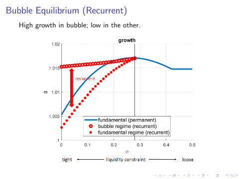
Bubble Equilibrium (Recurrent)

High growth in bubble; low in the other.

Bubble Equilibrium (Recurrent)Inter-temporal (inter-regime) substitution at work.

Recurrent v.s. Stochastic

Discrepancy in fundamental too.

Recurrent v.s. StochasticBoth wealth e¤ect and price e¤ect at work.

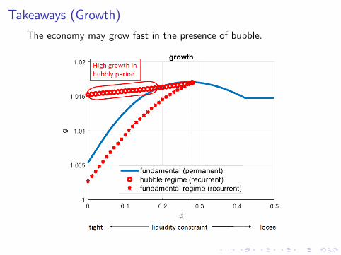
Takeaways (Growth)

The economy may grow fast in the presence of bubble.

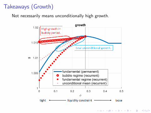
Takeaways (Growth)

Not necessarily means unconditionally high growth.

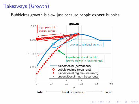
Takeaways (Growth)

Bubbleless growth is slow just because people expect bubbles.

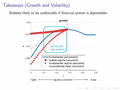
Takeaways (Growth and Volatility)

Bubbles likely to be undesirable if �nancial system is dependable.

Takeaways (Growth and Volatility)

Bubbles can be desirable if �nancial system is weak.

Takeaways (Growth and Volatility)

Seemingly puzzling views not a puzzle in our model.

Estimation

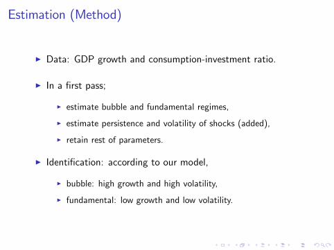
Estimation (Method)

I Data: GDP growth and consumption-investment ratio.

I In a �rst pass;

I estimate bubble and fundamental regimes,

I estimate persistence and volatility of shocks (added),

I retain rest of parameters.

I Identi�cation: according to our model,

I bubble: high growth and high volatility,

I fundamental: low growth and low volatility.

Estimation (U.S.)Regime switches from bubble!fundamental!bubble.

1960 1980 2000

0.2

0.4

0.6

0.8

Prob of Bubble

1960 1980 2000­1

­0.5

0

0.5

1

0.2

0.3

0.4

0.5

Productiv ity Shock

LevelVolatility

1960 1980 2000

­0.4

­0.2

0

0.2

0.4

0.6

0.1

0.15

0.2

Preference Shock

LevelVolatility

Estimation (Japan)Bubbles in the late 80s, the mid 90s, and very recent years.

1965 1970 1975 1980 1985 1990 1995 2000 2005 20100

0.1

0.2

0.3

0.4

0.5

0.6

0.7

0.8

0.9

1

Conclusion

I Recurrent bubbles.

I Two-way dynamic e¤ects (b f and f b).

I Super-hysteresis.

I Structural estimation.

Appendix

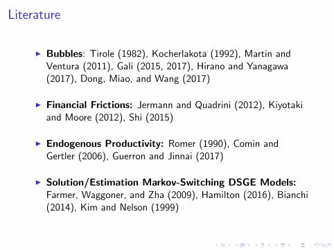
Literature

I Bubbles: Tirole (1982), Kocherlakota (1992), Martin andVentura (2011), Gali (2015, 2017), Hirano and Yanagawa(2017), Dong, Miao, and Wang (2017)

I Financial Frictions: Jermann and Quadrini (2012), Kiyotakiand Moore (2012), Shi (2015)

I Endogenous Productivity: Romer (1990), Comin andGertler (2006), Guerron and Jinnai (2017)

I Solution/Estimation Markov-Switching DSGE Models:Farmer, Waggoner, and Zha (2009), Hamilton (2016), Bianchi(2014), Kim and Nelson (1999)

Parameter Values

Parameter Value Calibration Targetβ 0.99 Exogenously Chosenα 0.4 Capital Share=0.4

fraction of investors 0.05 Exogenously ChosenIES 1 Exogenously Chosen

elasticity of δ0 (ut ) 0.33 Exogenously Chosenδ (1) 0.025 Annual Depreciation=0.10

η 2.78 Labor Supply=0.25A 0.30 Rental Rate of Capital=0.05

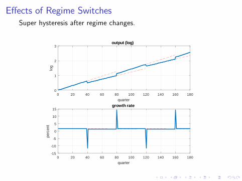
E¤ects of Regime SwitchesSuper hysteresis after regime changes.

0 20 40 60 80 100 120 140 160 180quarter

0

1

2

3lo

g

output (log)

0 20 40 60 80 100 120 140 160 180quarter

­15

­10

­5

0

5

10

15

perc

ent

growth rate

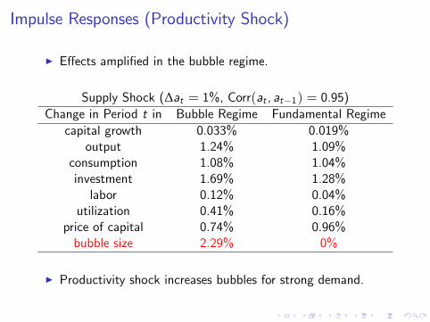
Impulse Responses (Productivity Shock)

I E¤ects ampli�ed in the bubble regime.

Supply Shock (∆at = 1%, Corr(at , at�1) = 0.95)Change in Period t in Bubble Regime Fundamental Regime

capital growth 0.033% 0.019%output 1.24% 1.09%

consumption 1.08% 1.04%investment 1.69% 1.28%labor 0.12% 0.04%

utilization 0.41% 0.16%price of capital 0.74% 0.96%bubble size 2.29% 0%

I Productivity shock increases bubbles for strong demand.

Impulse Responses (Preference Shock)

I E¤ects ampli�ed in the bubble regime.

Demand Shock (∆bt = 1%, Corr(bt , bt�1) = 0.8)Change in Period t in Bubble Regime Fundamental Regime

capital growth -0.034% -0.024%output 0.03% 0.11%

consumption 0.31% 0.30%investment -0.78% -0.71%labor -0.22% -0.15%

utilization 0.39% 0.49%price of capital -0.53% -0.60%bubble size -0.87% 0%

I Preference shock reduces bubbles by making people impatient.