Tardi TjahajdiImage Processing and Expert Systems LaboratoryInformation and Communication Research Group

School of EngineeringUniversity of Warwick

Recovery of 3-Dimensional Scene Information from Video Images

2

Contents of the Talk

• Brief review of 3D object/scene reconstruction• Camera calibration• Structure from motion• Shape from Silhouette

3

3D Object Reconstruction Methods• Applications: robot navigation, obstacle recognition, digital

preservation of works of arts, etc.• Active vision: laser scanning, stereo with structured lighting• Volumetric reconstruction:

Space carving (Kutulakos & Seitz, 2000) Voxel colouring (Seitz & Dyer 1999)

4

3D Object Reconstruction Methods (continued)• Shape from stereo• Shape from Silhouette (SfS)

• Structure from motion (SfM)

SfS (Yemez & Schmitt, 2004)

SfM (Jebara, AzarbayejaniPentland,1999)

5

Camera calibration

• Determines camera parameters• Methods 1 using calibration

object– e.g., Tsai, 1987; Zhang, 2000

• Methods 2 using geometricinvariance of image features– e.g., Meng & Hu, 2003

• Methods 3: self-calibration- e.g., Pollefeys & van Gool, 1999

• Precision of calibration depends:– feature detection– camera model

• Parametric distortions– parametric deviations from pinhole

model: methods 1– parametric models for specific lenses

• fish-eye transform model, e.g., Basu& Licardie, 1995.

• field-of-view model, e.g., Devermay &Faugeras, 2001.

• Generic (non-parametric) distortions– e.g., Mohr, Boufama & Brand, 1993

6

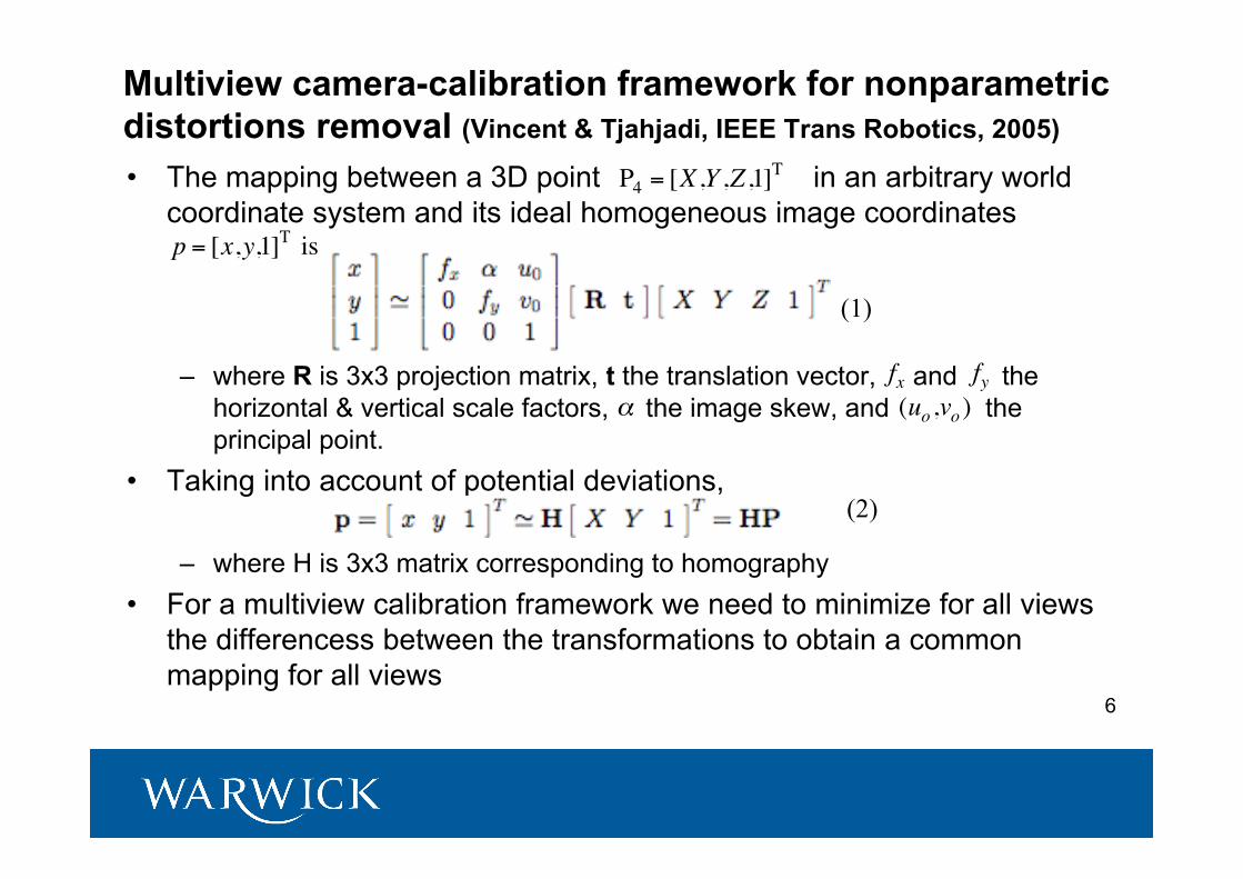
Multiview camera-calibration framework for nonparametricdistortions removal (Vincent & Tjahjadi, IEEE Trans Robotics, 2005)

• The mapping between a 3D point in an arbitrary worldcoordinate system and its ideal homogeneous image coordinates

– where R is 3x3 projection matrix, t the translation vector, and thehorizontal & vertical scale factors, the image skew, and theprincipal point.

• Taking into account of potential deviations,

– where H is 3x3 matrix corresponding to homography• For a multiview calibration framework we need to minimize for all views

the differencess between the transformations to obtain a commonmapping for all views

€

P4 = [X ,Y ,Z ,1]T

€

p = [x,y,1]T is

€

fx

€

fy

€

α

€

(uo ,vo )

(1)

(2)

7

• Define 2 affine transformations A and A’ for p and P such that (2)becomes

– where• For distortion corrections, use a virtual grid defined by P calibration

feature points . For each view compute the best homographywhich minimises the residual error associated with view j

– where are the observed sub-pixel coordinates of• For each view, the corrected (undistorted) points is given by

(3)

€

H = A-1H'A'

€

Pi

€

Hj

€

˜ p ij

€

Pi

€

˜ p iH j

(4)

(5)

8

• The estimations are further refined by fusing the corrective distortionmaps obtained from different views into a common distortion map,applying this map to correct the distorted pixel coordinates.

• The corrective distortion vector is

– where and are sets of control vectors, areB-spline basis function in u & v directions respectively

• The best B-spline surfaces that fit the estimated corrective distortions is given by the residual error

• The distortion vectors are given by the 2 distortion B-spline surfaces.The remaining intrinsic & extrinsic parameters are initialised usingBouguet’s solution on the currently undistorted pixel coordinates.

(6)

€

BH zk,l

€

BH zk,l

€

˜ p iH j− ˜ p i

j

(7)€

N k (u( ˜ p ixj )) & M k (u( ˜ p iy

j ))

9

Results

• The parameter vector to optimize is

Distorted and corrected images.

10

Re-constructing 3D object from an image sequence• Involves correspondence estimation, structure & motion

analysis, surface reconstruction• Correspondence estimation (Redert, Hendricks & Biemond, 1999):

– characterises the apparent motion of an imaged scene relative to thecamera, either by the displacement of a discrete set of features or bythe instantaneous velocities of brightness patterns

– tracking a set of features: two-frame & long-sequence based• Feature-based structure & motion estimation (Jebara, Azarbayejani

& Pentland, 1999):– 2-frame; or iterative and recursive multi-frame– 1st, the rigid motion between the views is recovered; and 2nd, the

motion estimate is used to recover the scene structure.• Surface reconstruction:

– Define surfaces to pass through recovered 3D feature points

11

3D metric object modelling from uncalibrated imagesequences (Cadman & Tjahjadi, IEEE Trans SMC, 2004)

System architecture Interactions between system modules

12

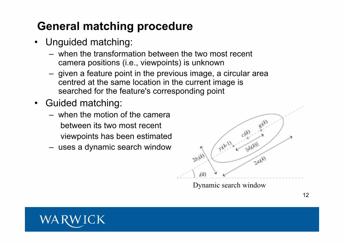
General matching procedure• Unguided matching:

– when the transformation between the two most recentcamera positions (i.e., viewpoints) is unknown

– given a feature point in the previous image, a circular areacentred at the same location in the current image issearched for the feature's corresponding point

• Guided matching:– when the motion of the camera between its two most recent viewpoints has been estimated– uses a dynamic search window

Dynamic search window

13

Corner tracking

• Initial corner matching: unguided matching to give ≥ 8 matched points• Additional corner matching: expected image locations of unmatched feature

points are used to guide matching• Pseudo corner matching and expiration: to handle disappearance, occlusion

& unsuccessful detection of corners• Inclusion of new corners: guided matching on original sets of feature points

and all expired pseudo corners using more lenient thresholds

14

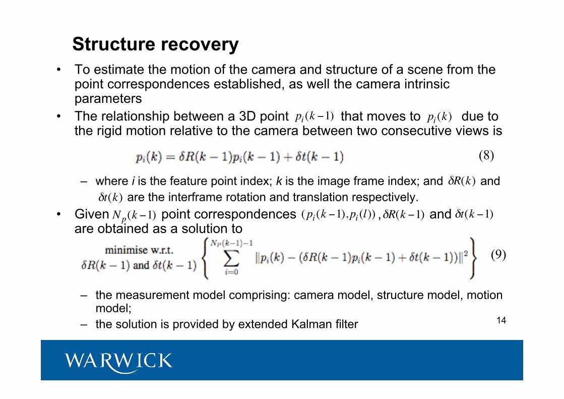
Structure recovery• To estimate the motion of the camera and structure of a scene from the

point correspondences established, as well the camera intrinsicparameters

• The relationship between a 3D point that moves to due tothe rigid motion relative to the camera between two consecutive views is

– where i is the feature point index; k is the image frame index; and and are the interframe rotation and translation respectively.

• Given point correspondences , andare obtained as a solution to

– the measurement model comprising: camera model, structure model, motionmodel;

– the solution is provided by extended Kalman filter

€

pi (k −1)

€

pi (k)

(8)

€

δR(k)

€

δt(k)

€

Np(k −1)

€

(pi(k −1),pi (l))

€

δR(k −1)

€

δt(k −1)

(9)

15

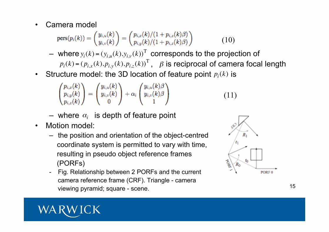
• Camera model

– where corresponds to the projection of , is reciprocal of camera focal length

• Structure model: the 3D location of feature point is

– where is depth of feature point• Motion model:

– the position and orientation of the object-centred coordinate system is permitted to vary with time, resulting in pseudo object reference frames (PORFs)- Fig. Relationship between 2 PORFs and the current camera reference frame (CRF). Triangle - camera viewing pyramid; square - scene.

€

yi (k) = (yi,u(k),yi,v (k))T

€

pi (k) = (pi,x (k),pi,y (k),pi,z (k))T

(10)

€

β

(11)

€

αi

€

pi (k)

16

Surface reconstruction• A recursive framework which incorporates a recursive score (indicating

the likelihood of any 2 feature points begin adjacent to one another onthe true surface) is used to estimate the complete topology of theimaged scene.

• Corner connectivity

– where is a directness score and denotes thenumber of frames in which both features have appeared together

– If greater than threshold ⇒ a potential edge• Constrained triangulation

– Beginning with a convex hull enclosing the object feature points, thetriangulated surface mesh is iteratively refined to ultimately yield aconstrained triangulation that can produce views consistent with theoriginal images of the scene.

– Visibility constraint: none of the surface’s visible facets should obscure orbe occluded by a potential edge.

(12)

€

dir(yi (k),yn(k))

€

λi,n(k)

17

Example results• Evolution of the surface overlaying recovered structure of a simulated object

• Recovering an object model from a raytraced box sequence

18

Example results• Recovering an object model from the MOVI sequence

• Recovering an object model from the hotel sequence

19

Shape from silhouette (SfS) techniques• 3D visual hull: intersection of multiple 3D cones that are created by

backprojection of 2D silhouettes of different views of an object onto 3Dspace.

• Octree: constructed by projecting an initial bounding cube (whichencloses an object in 3D space) onto multiple images of the object takenat different views, and splitting the cube into eight octants if theprojection intersects a silhouette

• Octants: outside, inside or intersection• Marching Cube (MC) (Lorensen & Cline, 1987):

– estimates surface triangles from intersection octants, and the location of thetriangles are determined by the configuration of inside vertices of anintersection octant

– MC generated surface may contain unexpected holes or discontinuities dueto: connectivity of octants, ambuiguity of MC algorithm, errorneous cameracalibration, and imperfect silhouette images.

20Images Silhouettes Octree

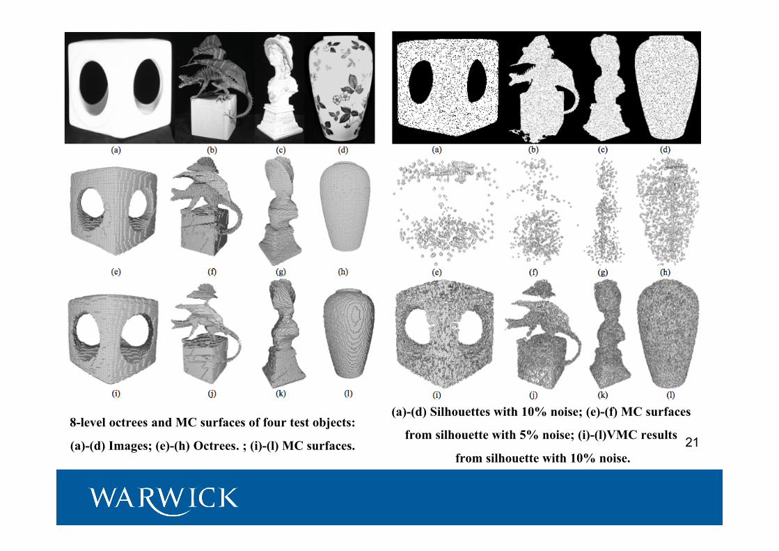
218-level octrees and MC surfaces of four test objects:

(a)-(d) Images; (e)-(h) Octrees. ; (i)-(l) MC surfaces.

(a)-(d) Silhouettes with 10% noise; (e)-(f) MC surfaces

from silhouette with 5% noise; (i)-(l)VMC results

from silhouette with 10% noise.

22

Surface reconstruction• MC

– assumes that intersection octants may include an actual surfacewhich crosses an edge joining two vertices of a surface octant withopposite status, i.e., inside and outside

– erroneous decision on an inside vertex supersedes other statusespreviously defined in other silhouettes ⇒ lost of surface patches

• Voting MC (VMC) (Yemez & Schmitt, 2004)

– counts the number of cases classified as outside and identifies anoutside vertex if the vote is greater than a threshold

• Delaunay Triangulation (DT) (Aurenhammer, 1991)

– constructs a convex surface by defining tetrahedrons from 3D points.– characterises each tetrahedron by not allowing any point within its

circumsphere

23

Local hull-based surface reconstruction (Shin &Tjahjadi, IEEE Trans IP, 2008)

Overview of surface construction process

24

3D objects & volumetric data slicing• 3D object properties

– Connectivity: surface of an object should cover the objecttightly without any unattached object segments

– Continuity: a shape of local convexity is similar to adjacentconvexity if they are connected ⇒ object needs to besliced infinitesimally

• Uses best VMC vertices• Uses octree vertices to define a local convexity• Quantized octree slice

– every four points are from the same octant– a binary image plane where a nonzero point represents an

octant– of a non-convex object can have multiple clusters that are

linked 8-neighbouring points• Quantized MC slice : decision on clustering and

connecting of clusters is based on a Bayesian rule anda priori information from the quantised octree slice (a) Octree; (b) octree slices

€

Simcq

€

Siocq

25

Identifying a local convexity• A local convexity is identified by: clustering

on and connecting clusters between slices.Given a cluster conditional pdf , theproblem of clustering is solved by searching forthe maximum probability. ( -test data, -class i)

• Using Parzen density estimator

• Cluster decision function

• Decision function for connecting a cluster

• Correlation coefficient between CID andTID’s:

(a) 3D pdf cube containing every clusterconditional pdf in a quantised MC slice.(b) Part of a tree table from slice 4 to 7.

€

Simcq

€

p(r t | ci )

(13)

(14)

(15)

(16)

€

r t

€

ci

€

nj - number of data in cluster j

26

Local surface construction• A local convexity is defined by two

connected clusters in different slices• If an object is not convex, a local

convexity can have multipleconnections

• Divide multiple connections into n 1:1connections with an appropriatedivision so as to minimise possibleduplication of surface patches in thecommon area

• The division is done along the bestrepresentative vector of the multipleclusters (determined using eigenanalysis) and according to thenormalised data distribution along thisvector.

1:n branching case. To avoid smoothing, the cluster is divided into 3 subregions, ,

and on the projection of the eigen vector V' and n 1:1 connections are made.

€

R2

€

R3

€

R4

€

C1

27

Results

(a)-(d) test objects: burner, dragon, bust, vase. (e)-(f) the reconstructed surfaces.

28

29

Thank you for your attention.

Any questions?